JESRT: 8(11), November, 2019 ISSN: 2277-9655 I ...ijesrt.com/issues /Archive-2019/November-2019/4.pdf · HVDC transmission system main problem arises due to line to ground fault

International Journal of Engineering Sciences &Research

Technology (A Peer Reviewed Online Journal)

Impact Factor: 5.164

IJESRT

Chief Editor Executive Editor

Dr. J.B. Helonde Mr. Somil Mayur Shah

Website: www.ijesrt.com Mail: [email protected] O

IJESRT: 8(11), November, 2019 ISSN: 2277-9655

I X

http://www.ijesrt.com/

mailto:[email protected]

ISSN: 2277-9655

[Patel, et al., 8(11): November, 2019] Impact Factor: 5.164

IC™ Value: 3.00 CODEN: IJESS7

http: // www.ijesrt.com© International Journal of Engineering Sciences & Research Technology

[36]

IJESRT is licensed under a Creative Commons Attribution 4.0 International License.

IJESRT INTERNATIONAL JOURNAL OF ENGINEERING SCIENCES & RESEARCH

TECHNOLOGY

FAULT LOCATION ESTIMATION FOR A BIPOLAR HVDC TRANSMISSION

LINE USING DIFFERENT BACK PROPAGATION ALGORITHMS OF ANN Ms. Khushboo Patel*1

, Mr. Deepak Bhataniya2 & Mr. Tarun Joshi3

*1M. Tech Scholar in Power Electronics, JIT Borawan, Khargone (M.P) 2&3Asst. Prof. in Electrical & Electronics Dept. JIT Borawan, Khargone (M.P)

DOI: 10.5281/zenodo.3542450

ABSTRACT In electrical transmission system uninterrupted supply is a primary demand from system. But every system

under go some type of situation where supply gets disconnected for some time based on severity of problem. In

HVDC transmission system main problem arises due to line to ground fault. Now the first step to resolve this

situation is to locate the exact location of fault occurrence. During this situation for a line long enough, it is very

difficult to manually check the whole because that will take long time. Hence a technique is to be derived which

has the ability to find the location so as to do the required maintenance as soon as possible and continue the

supply again. In this work an attempt is made to resolve this problem with the help of artificial neural network.

Two different algorithms of ANN are utilized in this work to calculate fault location of Bipolar HVDC

transmission line. This a bipolar HVDC transmission line is simulated for fault at a step of 1 km in

PSCAD/EMTDC software and data of both sending end and receiving end is collected. This data is input data

for Neural Network. In the present study a line of DC voltage of 500kV 816 km is taken. This line is a

prototype of India first bipolar line i.e. Rihand-Dadri HVDC line. After collection of data further modelling of

neural network model is done in neural network toolbox in MATLAB software. The results show that BR will

give more accurate results than LM thus proving to be more efficient method.

KEYWORDS: Fault location Detection, Artificial Neural Network, Levenberg–Marquardt(LM), Bayesian

Regularization(BR), Bipolar HVDC, MATLAB, PSCAD/EMTDC.

1. INTRODUCTION Transmission system plays the vital role in connecting generation station to load. It has the responsibility to

supply continuous power from one and two others. Any type of damage to transmission line will lead to an

interruption in power supply but in the present era of power system deregulation providing good power quality

with continuous supply is main its main priority of all electric utility companies. Hence for this reason focus

should be paid in the field of system protection and a proper planning is expected to deal with any unwanted

situation.

Relay and circuit breakers play key part in preventing system during any fault condition. Faults are responsible

for creating system malfunctioning and their immediate diagnosis is expected is expected to increase reliability.

Normally distance relays are used for locating fault. The working of distance relay is based upon the measured

value of impedance between fault point and relay location (that is ratio of voltage and current between these two

points). Now this should be giving accurate results, but due to the presence of series capacitor banks for

compensation problem will somehow tarnish the accuracy of relay.

Umar Saleem et.alin [20] has discussed a new method to predict fault location of a HVDC transmission line

using DWT technique. The author utilised this tool to findthe information form data observed and based on that

it has predicted the fault location. Author has done the decomposition of signals for 3rd level, having 3 detail

coefficients and a normalise coeffiient which when conpared with treshhold value will give the required

information of fault location. Author has tested the model for several fault location and found result satisfactory.


http://creativecommons.org/licenses/by/4.0/


ISSN: 2277-9655




[37]


Nabamita Roy & Kesab Bhattacharya [5] has presented a technique for detecting fault, classifying it had then

forecasting fault location. Values of feature is used for both classification and locating fault in this work. Author

has concluded that above following techniques includes BPNN techniques has developed a model which has

great speed of computation and very high accuracy.

Liang Yuansheng, Wang Gang, and Li Haifeng [6] has discuss a noble algorithm to detect fault location. Author

has performed a mix of travelling wave theory and Bergeron times domain fault location method. The value of

voltage and current from both sides is taken as input parameters. In this study a self-adopted filter is also utilized

which has ultimately improved performance of the algorithm.

S. F. Alwash, Member, V. K. Ramachandara murthy, and N. Mithulananthan [8] has developed an algorithm for

identification of all shunt type fault location. This work mainly presented a scheme where author has used

impedance method for fault location. This method is tested for IEEE 34 bus distribution system designed and

simulated in PSCAD/EMTDC software. In the study author has computed a method which has capability to

identify faults location irrespective of type of shunt fault.

Jae-Do Park, Member, IEEE, Jared Candelaria, Liuyan Ma, and Kyle Dunn [9] a DC microgrid system’s fault

location technique is proposed. In this work author has used intelligent electronic devices for the controlling

and monitoring all nodes. The author has successfully implemented proposed algorithm/technique both in

hardware and simulation experimentally.

M Ramesh, A. Jaya Laxmi [10] has presented an overview of various intelligent technique for detecting fault in

HVDC. In study author has discussed drawbacks of primitive fault detection techniques in HVDC. Then author

has provided an overview to various Artificial intelligent techniques in view to identify fault of HVDC

transmission system.

Eisa Bashier M. Tayeb, Orner AI Aziz Al Rhirn [11] discussed that in power system are always exposed to

abnormal conditions, which are the reason for the damage of transmission line and other electrical equipment’s

of power system. These abnormalities are termed as faults. These faults are required to be detected and

classified for better performance of transmission line.

2. METHODOLOGY Following techniques are utilized in present work for the purpose of fault location estimation:

Artificial Neural Networks (ANN):

The evolution of ANN has been dated way back in 1980’s with the evolutions of computers. From the very

same process of evolution, the term artificial neural network is been derived. The word artificial is basically

used to denote the capability of this model to replicate the working of human brain. Usually machines possess

a property work according to pre-defined instruction saved in it. However, this is not how human works. The

brain of any human has the capacity to take decision based on its experience which we call training in

computers language. Hence, it gives capability to brain to take decision that too right in cases which are new to

it. Therefore, machine learning is a method by which we inherit this specialty of human biological thinking

system and try to replicate same in computer/machine.

Now let’s understand how human brain works to form exact algorithm which can give similar outputs. Brain

consist of billions of neurons, which are interconnected with each other. These interconnections have a certain

strength, which makes our memory storage. Based on these memories we take decision over everything in real

time. The strength of these connections depends mainly on signal from various cells/neurons situated in each

part of our body. These neurons continuously send signal according to sense organs response to brain in the

form of electromagnetic pulses. These pulses are passed to brain through a series of chain of cells linking brain

with sense organs. These chains of cells have two responsibility to transfer signal from one part of body to other

and second to modify the signal in such a manner that brain will take the decision instantaneously.




ISSN: 2277-9655




[38]


Now the objective of formation of neural network is to reproduce the same scenario in computer based upon

programming, algorithms, processor and memory, which is discussed in detail in next section.

Levenberg–Marquardt (LM) Algorithm: The algorithm used in this work is Levenberg–Marquardt (LM)

Algorithm which a type of back propagation algorithm. The reason behind using this algorithm is due to its

exceptional ability to extract information from a nonlinear data with great stability which keeping speed of

convergence intractably high. The algorithm is a combination of two different algorithms proposed by two

mathematicians Levenberg and Marquardt and hence the named over them. The drawback of prior one is

remove by the advancement of second. The equation were derived back in mid-20th century for the sake of 1st

order error reduction purpose. However, with the invention of computers and high-level computation problem

this algorithm is evolved in to a great tool for time series forecasting. When the performance function has the

form of a sum of squares, then the Hessian matrix can be approximated and the gradient can be computer as

(1)

(2)

Where is the Jacobian matrix for kth input, which contains first order derivatives of the network errors with

respect to the weights and biases, 𝑒 is a vector of network errors. The Jacobian matrix can be computed

through a standard backpropagation technique that is much less complex than computing the Hessian matrix.

[11]

The Levenberg –Marquardt algorithm is actually a blend of the steepest descent method and the Gauss–

Newton algorithm. The following is the relation for LM algorithm computation,

(3)

where ‘I’ is the identity matrix, Wk is the current weight, Wk+1 is the next weight, ek+1 is the current total

error, and ek is the last total error, μ is combination coefficient. [11] [12]

The combination coefficient μ is multiplied by some factor (β) whenever a step would result in an increased

ek+1 and when a step reduces ek+1, µ is divided by β. In this study, we used β=l0. When μ is large the

algorithm becomes steepest descent while for small μ the algorithm becomes Gauss-Newton. [11]




ISSN: 2277-9655




[39]


Fig.1 Flow chart of LM algorithm

Bayesian Regularization (BR) Algorithm: BRANNs are extra vigorous than usual back-propagation networks

and can lessen the necessity for long cross-validation. BR algorithm is a process that changes a nonlinear

regression into a “well- modelled” statistical problem in the means of a ridge regression. In this algorithm

regularization is used to improve the network by optimizing the performance function (F(𝜔)). The performance

function F(𝜔) is the sum of the squares of the errors of the network weights (Ew) and the sum of squares error

of the data (𝐸D) [13] [14]:

(4)

Where, (5)

Both 𝛼 and 𝛽 are the objective function parameters. In the BR framework, the weights of the network are

viewed as random variables, and then the distribution of the network weights and training set are considered as

Gaussian distribution. The 𝛼 and 𝛽 factors are defined using the Bayes’ theorem. The Bayes’ theorem relates

two variables (or events), A and B, based on their prior (or marginal) probabilities and posterior (or conditional)

probabilities as [15]:




ISSN: 2277-9655




[40]


Fig.2 Flow chart of BR algorithm

(6)

Where P(A|B) is the conditional probability of event A, depending on event B, P(B|A) the conditional

probability of event B, depending on event A, and P(B) the previous probability of event B. In order to get the

best values of weights, performance function F(𝜔) (11) needs to be minimized, which is the equal to

maximizing the following probability function given as:

(7)

Where 𝛼 and 𝛽 are, the factors on which value of performance function is dependent and is the one which is

needed be to optimized, M is the particular neural network architecture, D is the weight distribution, P (𝐷|𝑀) is

the normalization factor, 𝑃 (𝐷|𝛼, 𝛽, 𝑀) is the likelihood function of D for given 𝛼, 𝛽, M and 𝑃 (𝛼, 𝛽|𝑀) is the

unvarying prior density for the regularization parameters.




ISSN: 2277-9655




[41]


Fig. 3: Working model of an ANN

The presentneural network consist of five input neuron,30-20 hiddenlayer neuronss and one output neurons as

shon in above figure.

3. MODELDESIGNAND DATA COLLECTION First stage of present work is to collect data for neural network training and testing. For this a bipolar HVDC

transmission line is simulated for fault at a step of 1 km in PSCAD/EMTDC software and data of both sending

end and receiving end is collected. This data is input data for Neural Network. In the present study a line of DC

voltage of 500kV 816 km is taken. This line is a prototype of India first bipolar line i.e. Rihand-Dadri HVDC

line.

Fig. 4: 500kV HVDC Bipolar line model in PSCAD




ISSN: 2277-9655




[42]


In ANN stage we will feed input data to input layer of present designed model and target is fitted to output

layer. We have used LM and BR training algorithm for training. It is this stage in which model is prepared and

value of weights are optimized for better performance according to input and target data samples.

Fig. 5: GUI of ANN during training

The below figure shows a training GUI of neural network, which will give all details of related to training. We

have taken 30-20 hidden layer neurons 6 input layer neurons and 1 output layer neuron.




ISSN: 2277-9655




[43]


RESULTS With BR >>

Fig. 6: Training states employing the proposed model using LM training

Figure 6 explains the training states for train using BR algorithm. The figure is devided in five parts.At top

gradient is shown and second graph shows value of mu and the third graph gives value Num parameters. Fourth

graph gives information of sum square parameter. Fifth graph gives information of validation states.




ISSN: 2277-9655




[44]


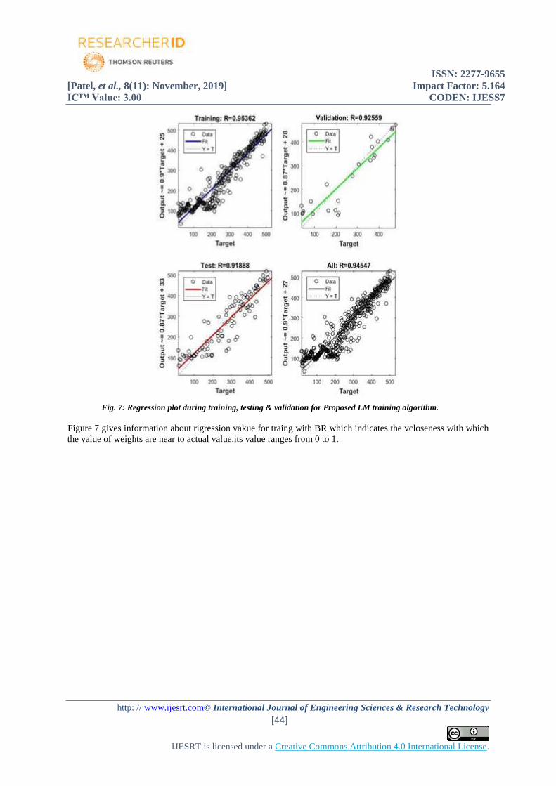
Fig. 7: Regression plot during training, testing & validation for Proposed LM training algorithm.

Figure 7 gives information about rigression vakue for traing with BR which indicates the vcloseness with which

the value of weights are near to actual value.its value ranges from 0 to 1.




ISSN: 2277-9655




[45]


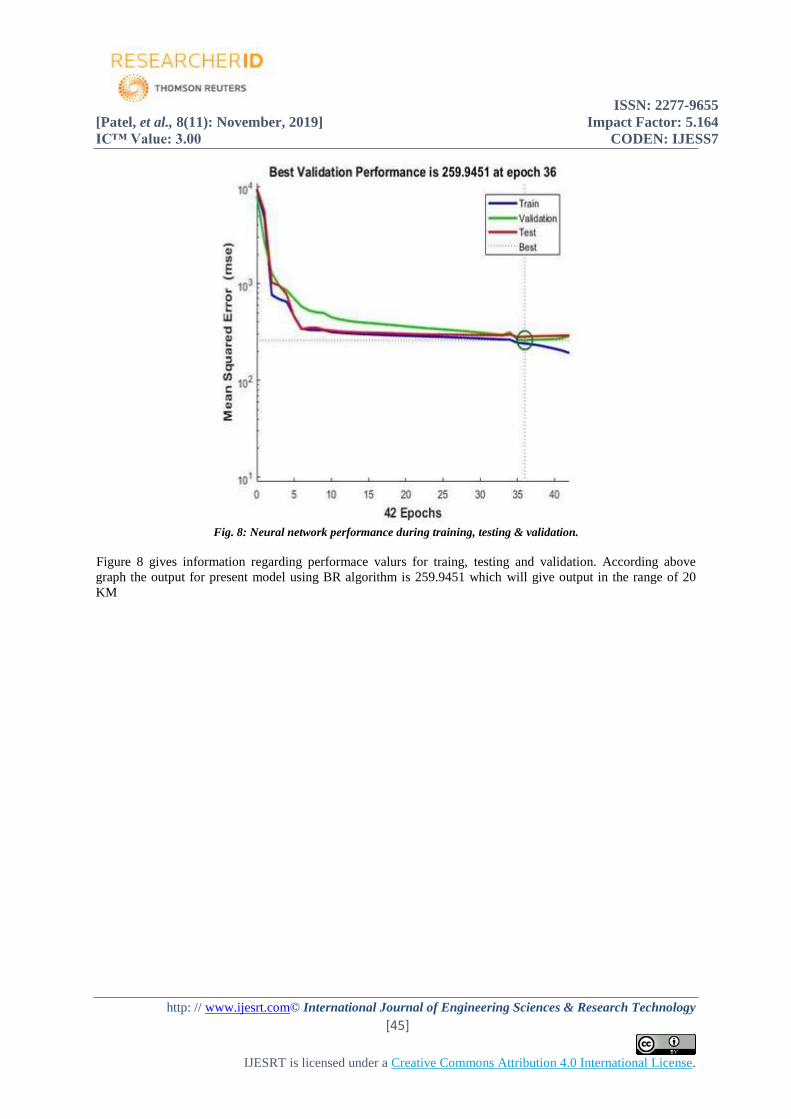
Fig. 8: Neural network performance during training, testing & validation.

Figure 8 gives information regarding performace valurs for traing, testing and validation. According above

graph the output for present model using BR algorithm is 259.9451 which will give output in the range of 20

KM




ISSN: 2277-9655




[46]


With LM>>

Fig. 9: Training states employing the proposed model using LM training

Figure 9 explains the training states for traingusing LM algorithm. The figure is devided in to three parts. At top

gradient is shown and second graph shows value of mu and the third graph gives value of validation states




ISSN: 2277-9655




[47]


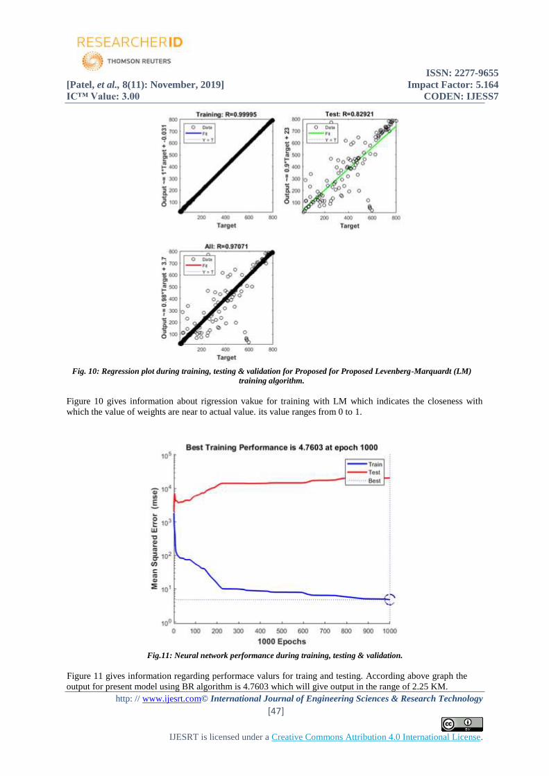
Fig. 10: Regression plot during training, testing & validation for Proposed for Proposed Levenberg-Marquardt (LM)

training algorithm.

Figure 10 gives information about rigression vakue for training with LM which indicates the closeness with

which the value of weights are near to actual value. its value ranges from 0 to 1.

Fig.11: Neural network performance during training, testing & validation.

Figure 11 gives information regarding performace valurs for traing and testing. According above graph the

output for present model using BR algorithm is 4.7603 which will give output in the range of 2.25 KM.




ISSN: 2277-9655




[48]


4. CONCLUSION In the present research, an attempt is made to predict fault location for a HVDC link using ANN models by

utilizing receiving end and sending end data to train ANN model. The model developed is able to predict fault

location accurately.

The developed ANN model with the configuration of 6-30-20- 1 is trained using LM back propagation

algorithm, proving to be efficient method.

REFERENCES [1] Jenifer Mariam Johnson and Anamika Yadav, “Fault Location Estimation in HVDC transmission line

using ANN” First International Conference on Information and Communication Technology for

Intelligent Systems: Volume 1, Pages 205-211, Springer, 2016.

[2] Sunil Singh D. N. Vishwakarma, “ANN and Wavelet Entropy based Approach for Fault Location in

Series Compensated Lines”, 2016 International Conference on Microelectronics, Computing and

Communications (MicroCom), Pages 1-5, IEEE, 2016.

[3] Ankita Nag and Anamika Yadav, “Artificial Neural Network for Detection and Location of Faults in

Mixed Underground Cable and Overhead Transmission Line”, International Conference on

Computational Intelligence and Information Technology, CIIT, kochi, pp 1-10, 2016.

[4] Qingqing Yang, Jianwei Li, Simon Le Blond, Cheng Wang, “Artificial Neural Network Based Fault

Detection and Fault Location in the DC Microgrid”, Energy Procedia 103, pp 129 – 134,

ScienceDirect, 2016.

[5] Alexiadis, M.C., Dokopoulos, P.S., Sahasamanoglou, H.S., Manousaridis, I.M.: Short-term forecasting

of wind speed and related electrical power. Solar Energy Volume 63, Pages 61–68, 1998.

[6] Giorgi, M.G.D., Ficarella, A., Tarantino, M. “Error analysis of short term wind power prediction

models, Appl. Energy 88, pp. 1298–1311, 2011.

[7] P. M. Fonte, Gonçalo Xufre Silva, J. C. Quadrado, Wind Speed Prediction using Artificial Neural

Networks, 6th WSEAS Int. Conf. on Neural Networks, Lisbon, Portugal, June 16-18, pp. 134-139,

2005.

[8] D. Marquardt, An algorithm for least-squares estimation of nonlinear parameters, SIAM J. Appl.

Math., Vol. 11, pp. 431–441, 1963.

[9] K. Levenberg, A method for the solution of certain problems in least squares, Quart. Appl. Mach., vol.

2, pp. 164– 168, 1944.

[10] A Method of Accelerating Neural Network Learning, Neural Processing Letters, Springer, pp. 163–

169, 2005.

[11] M. T. Hagan and M. B. Menhaj, Training feedforward networks with the Marquardt algorithm, IEEE

Transactions on Neural Networks, vol. 5, no. 6, pp. 989–993, 1994.

[12] Bogdan M. Wilamowski and Hao Yu, Improved Computation for Levenberg–Marquardt Training,

IEEE Transactions on Neural Networks, Vol. 21, No. 6, Page(s): 930 – 937, 2010.

[13] Mackay, D.J.C., Bayesian interpolation, Neural Computation, Vol. 4, pp 415-447, (1992).

[14] Zhao Yue; Zhao Songzheng; Liu Tianshi, Bayesian regularization BP Neural Network model for

predicting oil-gas drilling cost, Business Management and Electronic Information (BMEI), 2011

International Conference on 13-15, vol.2, pp. 483-487, 2011.

[15] M. S. Miranda, and R. W. Dunn, One-hour-ahead wind speed prediction using a Bayesian

methodology, IEEE Power Engineering Society General Meeting, pp. 1-6, 2006.

[16] Nabamita Roy & Kesab Bhattacharya, “Detection, Classification, and Estimation of Fault Location on

an Overhead Transmission Line Using S-transform and Neural Network”, Electric Power Components

and Systems, 43(4), pp 461–472, Taylor & Francis, 2015.

[17] Liang Yuansheng, Wang Gang, and Li Haifeng, “Time- Domain Fault-Location Method on HVDC

Transmission Lines Under Unsynchronized Two-End Measurement and Uncertain Line Parameters”,

IEEE Transactions on Power Delivery 1, pp: 1031 – 1038, 2015.

[18] Pu Liu, Renfei Che, Yijing Xu, Hong Zhang, “Detailed Modeling and Simulation of ±500kV HVDC

Transmission System Using PSCAD/EMTDC”, IEEE PES Asia-Pacific Power and Energy Engineering

Conference (APPEEC), pp 1- 3, IEEE, 2015




ISSN: 2277-9655




[49]


[19] S. F. Alwash, V. K. Ramachandaramurthy, and N. Mithulananthan, “Fault Location Scheme for Power

Distribution System with Distributed Generation”, IEEE Transactions on Power Delivery,pp 1187-

1195, 2014.

[20] UMAR SALEEM, USMAN ARSHAD, BILAL MASOOD, TALHA GUL, WAHEED AFTAB

KHAN, MANZOOR ELLAHI, “FAULTS DETECTION AND CLASSIFICATION OF HVDC

TRANSMISSION LINES OF USING DISCRETE WAVELET TRANSFORM”, IEEE 2018

INTERNATIONAL CONFERENCE ON ENGINEERING AND EMERGING TECHNOLOGIES

(ICEET), PP 1-6, 2018.




Documents

JESRT: 8(11), November, 2019 ISSN: 2277-9655 I ...ijesrt.com/issues /Archive-2019/November-2019/4.pdf · HVDC transmission system main problem arises due to line to ground fault