JESRT: 7(12), December, 2018 ISSN: 2277-9655 I ... /Archive-2018/December-2018/24.pdf3Faculty of Science and Technology, University of Kara, BP 404, Togo DOI: 10.5281/zenodo.2296359

International Journal of Engineering Sciences &

Research Technology (A Peer Reviewed Online Journal)

Impact Factor: 5.164

IJESRT

Chief Editor Executive Editor

Dr. J.B. Helonde Mr. Somil Mayur Shah

Website:www.ijesrt.com Mail: [email protected] O

IJESRT: 7(12), December, 2018 ISSN: 2277-9655

I X

http://www.ijesrt.com/

ISSN: 2277-9655

[Seyf-Laye * et al., 7(12): December, 2018] Impact Factor: 5.164

IC™ Value: 3.00 CODEN: IJESS7

http: // www.ijesrt.com© International Journal of Engineering Sciences & Research Technology

[222]

IJESRT INTERNATIONAL JOURNAL OF ENGINEERING SCIENCES & RESEARCH

TECHNOLOGY

NITROGEN TRANSFORMATION AND TRANSPORT MODELING IN

GROUNDWATER AQUIFERS USING SPREADSHEETS Alfa-Sika Mande Seyf-Laye1, 2, 3*, Ibrahim Tchakala2, Dougna Akpénè Amenuvevega2,3,

Djaneye-Boundjou G2, Moctar L. Bawa2, Honghan Chen1

1Beijing Key Laboratory of Water Resources Environmental Engineering, China University of

Geosciences (Beijing), Beijing 100083, China. 2Water Chemistry Laboratory, Faculty of Science, University of Lome, BP 1515, Togo.

3Faculty of Science and Technology, University of Kara, BP 404, Togo

DOI: 10.5281/zenodo.2296359

ABSTRACT Groundwater nitrogen pollution is a common problem and it poses a major threat to groundwater-based drinking

water supplies. In this study, a kinetic model is developed to study nitrification–denitrification reactions in

groundwater aquifers. A new reaction module for the reactive transport in one-dimension code is developed and

tested to describe the fate and transport of nitrogen species. The proposed model was developed to simulate

groundwater nitrate concentration. The model is later used to study the field-scale nitrogen transport and

transformations at a catchment area of Shenyang City. Modeling results are consistent, indicating that the

method provides a convenient for solving practical problems on nitrogen transport and transformation. The

developed model describing nitrification and denitrification reactions is a useful framework for simulating the

fate and transport of nitrogen species in groundwater aquifers.

KEYWORDS: Nitrogen; transportation, transformation; groundwater; modeling; spreadsheets.

1. INTRODUCTION Groundwater nitrogen pollution is a worldwide problem. In the process of three nitrogen transport, nitrification-

denitrification reaction occurs under certain hydrogeochemical condition, thus its concentration changed (Burt et

al 2006). At present, there are some difficulties on the quantitative prediction of nitrogen species in the process

of its transportation and transformation. The existing commercial groundwater numerical simulation software

can simulate the transportation of a variety of components at the same time, but have not provide the coupling of

nitrification and denitrification function. Despite some software (such as RT3D, Feflow) accomplished the

model secondary development function, but it requires the user must certain computer programing languages.

These simulation softwares are highly professional and technical requirements for the users are high, too.

One of the best tools for solving this problem is spreadsheet. One of the best tools for solving the PDE is

spreadsheet. There are many advantages of spreadsheets such as having numerical and visual feedback, fast

calculating capabilities. One of the most important advantages of spreadsheets is its graphical interface. The

solution obtained through the spreadsheet can easily be plotted at the same worksheet. Any changes in the input

parameters of the solution domain will be directly reflected to the graphical representation of the solutions.

Spreadsheets are user-friendly and easy to program. Several studies have been carried out using spreadsheets for

the last 10 years. In this modeling, on a spreadsheet it is not necessary to write out an equation in all cells to

carry out iterative calculations. Using copy and paste features of the spreadsheets, the equation can be copied to

other cells without writing the equations to all cells individually. When the equation pasted to all cells of the

solution domain, iterative calculation is started. It is carried out until the given number of iteration is finished or

maximum convergence criterion has been met. The main objective of this study is to develop a user- friendly

and flexible method to solve the one-dimensional transport and transformation mathematical model of nitrogen

species. (Mee-Sun et al, 1993, Halilkarahan, 2006; Clement, 2001)


ISSN: 2277-9655




[223]

2. MATERIALS AND METHODS 2.1 Nitrogen transformation concept

Mathematical model

2.1. Nitrogen transformations and transport

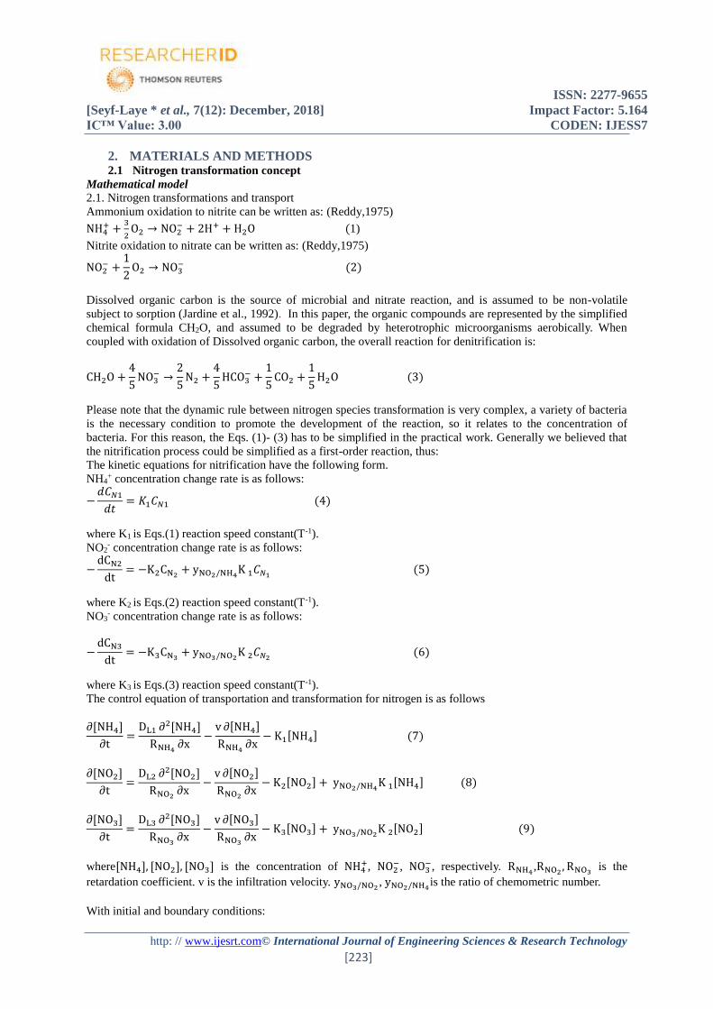
Ammonium oxidation to nitrite can be written as: (Reddy,1975)

NH4+ +

3

2O2 → NO2

− + 2H+ + H2O (1)

Nitrite oxidation to nitrate can be written as: (Reddy,1975)

NO2− +

1

2O2 → NO3

− (2)

Dissolved organic carbon is the source of microbial and nitrate reaction, and is assumed to be non-volatile

subject to sorption (Jardine et al., 1992). In this paper, the organic compounds are represented by the simplified

chemical formula CH2O, and assumed to be degraded by heterotrophic microorganisms aerobically. When

coupled with oxidation of Dissolved organic carbon, the overall reaction for denitrification is:

CH2O +4

5NO3

− →2

5N2 +

4

5HCO3

− +1

5CO2 +

1

5H2O (3)

Please note that the dynamic rule between nitrogen species transformation is very complex, a variety of bacteria

is the necessary condition to promote the development of the reaction, so it relates to the concentration of

bacteria. For this reason, the Eqs. (1)- (3) has to be simplified in the practical work. Generally we believed that

the nitrification process could be simplified as a first-order reaction, thus:

The kinetic equations for nitrification have the following form.

NH4+ concentration change rate is as follows:

−𝑑𝐶𝑁1

𝑑𝑡= 𝐾1𝐶𝑁1 (4)

where K1 is Eqs.(1) reaction speed constant(T-1).

NO2- concentration change rate is as follows:

−dCN2

dt= −K2CN2

+ yNO2/NH4K 1𝐶𝑁1

(5)


NO3- concentration change rate is as follows:

−dCN3

dt= −K3CN3

+ yNO3/NO2K 2𝐶𝑁2

(6)


The control equation of transportation and transformation for nitrogen is as follows

∂[NH4]

∂t=

DL1 ∂2[NH4]

RNH4∂x

−v ∂[NH4]

RNH4∂x

− K1[NH4] (7)

∂[NO2]

∂t=

DL2 ∂2[NO2]

RNO2∂x

−v ∂[NO2]

RNO2∂x

− K2[NO2] + yNO2/NH4K 1[NH4] (8)

∂[NO3]

∂t=

DL3 ∂2[NO3]

RNO3∂x

−v ∂[NO3]

RNO3∂x

− K3[NO3] + yNO3/NO2K 2[NO2] (9)

where[NH4], [NO2], [NO3] is the concentration of NH4+, NO2

−, NO3−, respectively. RNH4

,RNO2, RNO3

is the

retardation coefficient. v is the infiltration velocity. yNO3/NO2, yNO2/NH4

is the ratio of chemometric number.

With initial and boundary conditions:


ISSN: 2277-9655




[224]

where C1, C2, C3 is the concentration of NH4+, NO2

−, NO3− , respectively.

The solution domain of the problem is covered by a mesh of grid-lines

xi= iΔx, i = 0, 1, 2,..., M,

tn = nΔt, n= 0, 1, 2,..., N,

where xi and tn are parallel to the space and time coordinate axes. The constant spatial and temporal grid spacing

are Δx=L/M and Δt=T/N.

Consider the following approximations of the derivatives in the advection–diffusion equation which incorporate

time and space weights φ and θ as follows [3]:

where φ is a time weighting factor and θ is the spatial weighting factor.

Substituting Eqs. (12), (13) and (14) into Eq. (11)


ISSN: 2277-9655




[225]

One equation of the form of (15) is written for each active node, leading to a system of linear algebraic

equations. Note that the unknown concentration at any node at the new time level depends on the concentrations

at adjacent nodes at the new time level, which are also unknown. Thus, the system of linear algebraic equations

resulting from the implicit scheme must be solved simultaneously, using a direct matrix solution technique or an

iterative solution method.

This study uses iterative spreadsheet solution as

The solution of Eq. (11) is further analyzed as:

For φ= 1 and θ=1⁄2, Eq. (15) yields the implicit BTCS (Backward time centred space) - type finite difference

technique

Note that it is used for the spatial derivative in the advection term, the backward-difference form for the time

derivative and the centered-difference for the spatial derivative in the diffusion term. Eq. (21) is only first-order

accurate and incorporates numerical diffusion amounting to vkΔx/2.

Similarly, for φ= 1 and θ=0, Eq. (15) may be written as the upwind-type finite difference formula and for φ= 1/2

and θ=1/2, Eq. (5) may be written as the Crank–Nicolson type formula. To eliminate the numerical oscillations

and dispersion more efficiently, need to meet, Pe<2; Cr<1; Δx<αL (Lindstrom et al, 1992). This study was within

the range.


ISSN: 2277-9655




[226]

Model development

The model implementation is divided into rectangular grid intervals both in x direction and time dimension in

order to carry out the iterative spreadsheet calculations (see Fig. 1). In order to achieve the iterative calculations,

the maximum number of iterations and maximum error value need to be set be before simulations(“Office”-

“Excel Options”-“formula”-“iteration count”). In this study, we set 1000 and 0.0001, respectively.

It takes R1, R2, R3, D1, D2, D3, K1, K2, K3, Pe1, Pe2, Pe3, Cr1, Cr2, Cr3, v, Δx, Δt, θ and φ values as input

parameters.

Solution of model implementation is carried out based on Eq. (20) in the following spreadsheet format:

F3 = (-F2-$B$23*$B$18*(E2+G2-2*F2)/$B$2+$B$23*$B$14*($B$22*G2-$B$24*E2+$B$24*F2-

$B$22*F2)/$B$2+$B$9*F2*$B$13-$B$25*E3-$B$31*G3)/$B$28 (22)

where F3, which is an intersection of the six column (F) and third row (3), represents the concentration in cell.

Related terms are used in solving Eq. (20) has been shown in Eq. (22) as a spreadsheet format.

Before starting the simulation, firstly it is necessary to enter the initial and boundary condition values. After that,

Eq. (22) is written to the F3 cell. After the completion of this process, the formulas in the F3 cells are copied and

pasted to the relevant cell with the help of a basic macro and the iterative calculation is started. The sequence of

calculation is then repeated for the second and subsequent iterations, until the termεis less than the error

criterion at all nodes or the time index reaches the N value.

3. RESULTS AND DISCUSSION

3.1 Numerical applications

Take a continuous source in homogeneous isotropic groundwater system for example. Specific parameters are as

follows (Clement et al, 1998).

The values of the various parameters used are [NH4] =0.42, [NO2] =0, [NO3] =0, RNH4=1.6306, RNO2=1.0352,

RNO3=1.0352, DL1=221.9256, DL2=120.7776, DL3= 120.7776, v = 5.28 m/s, K1= 0.0874, K2=0.484, K3=0.002.

The space step and time step are taken to be Δx = 25 m and Δt = 1 s, respectively.

Fig2. Changing curve of concentration (T=5d) Fig3. Changing curve of concentration (T=15d)

Fig4. Changing curve of concentration (L=25cm) Fig5. Changing curve of concentration (L=100cm)

The analytical solution to the one-dimensional transport and transformation mathematical model of three

nitrogen is given as


ISSN: 2277-9655




[227]

From Fig.6, BTCS model gives very close results to the analytical solution. Therefore, the model can be used to

simulate three nitrogen transport and transformation problem.

Fig 6. Comparison of analytical and numerical solution (BTCS scheme)

4. CONCLUSION In this study, a mathematical model was developed to describe transformations and transport of nitrogen

compounds in a saturated groundwater aquifer. From the Comparison of analytical and numerical solution

(BTCS scheme), the model is feasible and it can provide a convenient tool for simulating the transportation and

transformation for nitrogen in groundwater. With the change of the input parameters, the change in the model

results can easily be observed graphically. Thus, the effect of the model parameters on the model accuracy,

stability can be seen visually. The model not only can simulate one-dimensional solute transport, but also can be

applied to two-dimensional case.

5. ACKNOWLEDGEMENTS This research was supported by the studies of safety evaluation and pollution prevention technology and

demonstration for groundwater resources in Beijing (D07050601510000) and Sate Science and Technology

Major Project for Water Pollution Controls and Treatment (2009ZX07424).

REFERENCES [1] Burt, T.P., Heathwaite, A.L., Trudgill, S.T.,Nitrate: Process,Patterns and Management. Wiley, New

York.1993

[2] Mee-Sun Lee, Kang-kun Lee, et al, .Nitrogen transformation and transport modelingin groundwater

aquifers. Ecological modeling, 2006.

[3] Halilkarahan.Implicit finite difference techniques for the advection–diffusion equation using

spreadsheets.Elsevier, 2006.

[4] Clement, T.P.,. Generalized solution to multispecies transport equations coupled with a first-order

reaction network. WaterResour. Res. 2001; 37 (1), 157–163.

[5] Reddy, K.R., Patrick, W.H. Effect of alternate aerobic and anaerobic conditions on redox potential,

organic matter decomposition and nitrogen loss in a flooded soil. Soil Biol. Biochem. 1975, 7, 87–94.

[6] Jardine, P.M., Dunnuvant, F.M., Selim, H.M., McCarthy, J.F., 1992. Comparison of models for

describing the transport of dissolved organic carbon in aquifer column. Soil Sci. Soc. Am. J. 56, 393–

401.

[7] Lindstrom, F.T., 1992. A mathematical model for the onedimensional transport and fate of oxygen and

substrate in a water-saturated sorbing homogeneous porous medium. Water

[8] Clement, T.P., Sun,Y., Hooker, B.S., Pertersen, J.N., 1998. Modelingmulti-species reactive transport in

groundwater aquifers. GroundWater Monit. Rem. 18 (2), 79–92.


Documents

JESRT: 7(12), December, 2018 ISSN: 2277-9655 I ... /Archive-2018/December-2018/24.pdf3Faculty of Science and Technology, University of Kara, BP 404, Togo DOI: 10.5281/zenodo.2296359