1

U N I V E R S I T Y O F C O P E N H A G E N

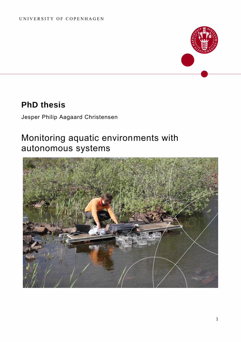
PhD thesis

Jesper Philip Aagaard Christensen

Monitoring aquatic environments with autonomous systems

2

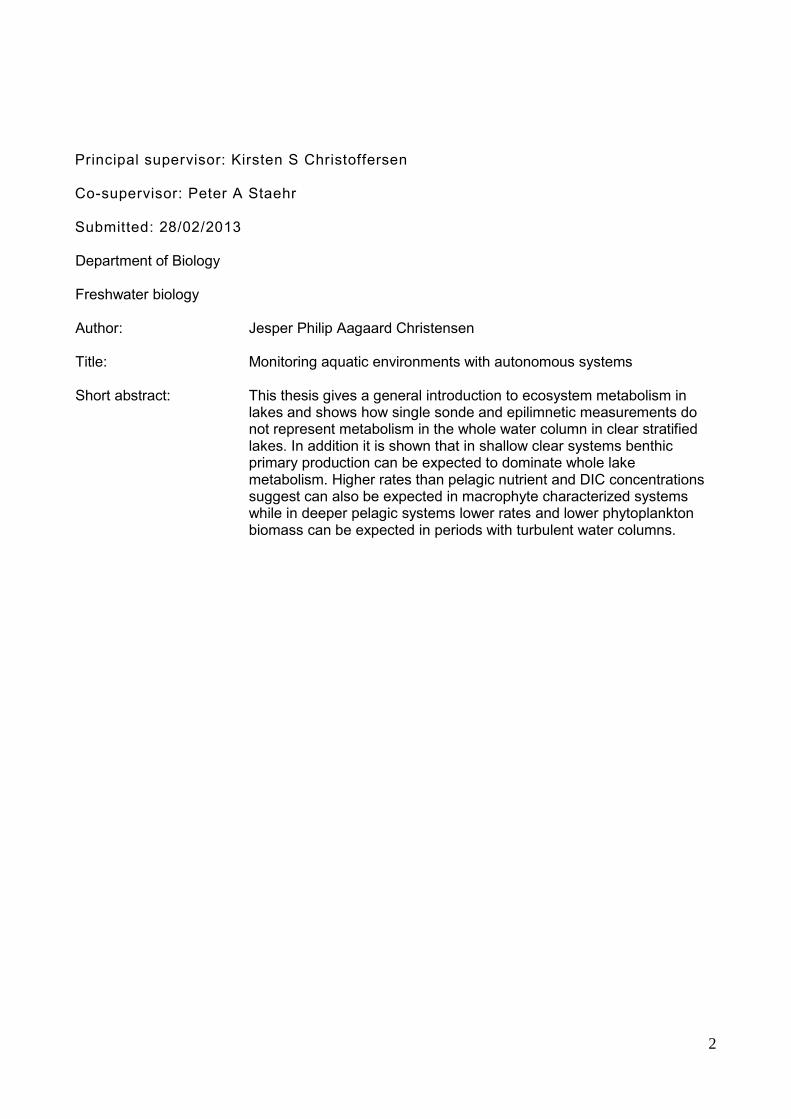
Department of Biology Freshwater biology Author: Jesper Philip Aagaard Christensen Title: Monitoring aquatic environments with autonomous systems Short abstract: This thesis gives a general introduction to ecosystem metabolism in

lakes and shows how single sonde and epilimnetic measurements do not represent metabolism in the whole water column in clear stratified lakes. In addition it is shown that in shallow clear systems benthic primary production can be expected to dominate whole lake metabolism. Higher rates than pelagic nutrient and DIC concentrations suggest can also be expected in macrophyte characterized systems while in deeper pelagic systems lower rates and lower phytoplankton biomass can be expected in periods with turbulent water columns.

Principal supervisor: Kirsten S Christoffersen

Co-supervisor: Peter A Staehr

Submitted: 28/02/2013

3

Preface

The content of this thesis includes part of the work I have been involved in during the last

three year as a PhD-student at the Freshwater Biological Laboratory. Four scientific manuscripts are

presented for evaluation. Two are already published or in press in Limnology and Oceanography

and Freshwater Biology respectively. One manuscript is in review at Limnology and Oceanography

and the last manuscript are being prepared for submission.

In addition I have worked on a climate change impact assessment analysis in the Baltic Sea

called Climate change impacts on marine biodiversity and habitats in the Baltic Sea published on

the web in collaboration with Danish metrological institute and Aarhus University

4

Contents

Abstract ........................................................................................................................ 5

Resume .......................................................................................................................... 6

Thesis objectives .......................................................................................................... 7

Introduction ................................................................................................................. 8

Thesis summary ......................................................................................................... 13

Estimating metabolism .............................................................................................. 17

Conclusions and perspective..................................................................................... 19

References .................................................................................................................. 20

Paper I ........................................................................................................................ 23

Paper II ....................................................................................................................... 38

Paper III ..................................................................................................................... 68

Paper IV ..................................................................................................................... 82

Acknowledgements .................................................................................................. 104

5

Abstract

High frequency measurements from autonomous sensors have become a widely used tool among

aquatic scientists. This report focus primarily on the use of ecosystem metabolism based on high

frequency oxygen measurements and relates the calculations to spatial variation, biomass of the

primary producers and environmental variables. The results can be formulated in three main

conclusions.

1) Primary production and respiration in stratified lakes are not evenly distributed in the water

column. Generally you can expect the net production to decreases with depth as gross primary

production (GPP) decreases with depth, unless it is a very clear lake, while respiration is relatively

stable. Metabolism estimates based on data from the epilimnion will only represent a minor

proportion of the whole lake metabolism under conditions of strong stratification and high water

transparency. At a low depth of the upper mixed layer (Zmix) and a euphotic zone (Zeu) which is

deeper than Zmix (Zeu> Zmix) GPP in epilimnion will most likely represent less than 80% of GPP

in the whole water column and respiration (R) in the epilimnion will most likely be less than 60%

of respiration integrated over the whole water column.

2) Physical water movement across the thermocline can account for around 50% of the variation

in the oxygen concentrations in metalimnion and up to 80% of the variation in oxygen

concentration in hypolimnion in a clear water, mesotrophic, polymictic lake. In contrast the oxygen

variations in epilimnion were primarily a result of metabolism and gas exchange with the

atmosphere, while only 10% of the variation was due to physical movement of water across the

thermocline.

3) Dense macrophyte populations in oligotrophic systems may have a higher GPP than expected

based on nutrient conditions in the water phase and in shallow systems the macrophytes can

completely dominate primary production. This was despite the fact that the plants in the studied

system were light-saturated most of the light hours and occasionally carbon limited. It was also

shown that the GPP and the total phytoplankton biomass in a nutrient-rich but deeper lake may be

below the expected level based on nutrient conditions when algal succession was regularly

interrupted due to repeated mixing events during an otherwise stratified period.

6

Resume

Høj frekvente målinger fra autonomt måleudstyr er blevet et udbredt værktøj blandt akvatiske

biologer. Denne rapport fokuserer primært på brugen af økosystem metabolisme baseret på høj

frekvente iltmålinger og tolker på beregningerne i relation til rummelig variation, primær

producenters biomasse og miljøvariable. Resultaterne kan formuleres i tre hovedkonklusioner.

1) Primær produktion og respiration i lagdelte søer er ikke ligeligt fordelt ned igennem

vandsøjlen. Generelt kan man forvente at netto produktionen falder med dybden da brutto

primærproduktionen (GPP) falder med dybden, med mindre søen er meget klarvandet, mens

respirationen er relativt stabil. Metabolisme beregninger fra epilimnion vil repræsentere en mindre

andel af hele søens metabolisme under forhold med stærk lagdeling og høj vandgennemsigtighed.

Ved en lav dybde af den opblandede zone (Zmix) og en eufotisk zone (Zeu) som er dybere en Zmix

(Zeu > Zmix) vil GPP i epilimnion sandsynligvis repræsenterer mindre end 80 % af hele

vandsøjlens primærproduktion og respirationen (R) i epilimnion vil sandsynligvis udgøre mindre

end 60 % af hele vandsøjlens respiration.

2) Fysisk vandbevægelse henover springlaget kan udgøre ca. 50 % af variationen i

iltkoncentrationerne i metalimnion og op til 80 % af iltvariationen i hypolimnion i en klarvandet,

mesotrof, polymiktisk sø. Til gengæld skyldes iltvariationerne i epilimnion primært metabolisme og

gasudveksling med atmosfæren, mens kun 10 % af variationenerne skyldes fysisk vandbevægelse

henover springlaget.

3) Tætte makrofyt bestande i oligotrofe systemer kan have en højere GPP end forventet baseret på

næringsforholdende i vandfasen og i lavvandet systemer kan de fuldstændig dominerer primær-

produktionen. Dette på trods af at planterne i det undersøgte system var lysmættede det meste af de

lyse timer og ind imellem var kulstofbegrænset. Samtidig blev det vist at GPP og den samlede

fytoplankton biomasse kan ligge under det forventelige baseret på næringsforholdende i en

næringsrig men dybere sø, når algesuccessionen bliver løbende afbrudt på grund af gentagende

opblandinger i løbet af den normalt lagdelte periode.

7

Thesis objectives

The main objective of the thesis was to explore the potential of environmental monitoring using

automated data logger systems deployed in lakes. During the thesis I have focused on data

acquisition, data analysis, as well as modeling of ecosystem metabolism, and evaluated the obtained

results in the context of other environmental parameters. During the thesis four main objectives

were explored:

1) Explore the technique of ecosystem metabolism estimation from diel oxygen curves

This part of my thesis aims to describe the level and daily to annual variations in metabolism of

temperate lakes. The metabolism and physical state of the temperate lakes were described based on

physical parameters that were obtained through autonomous high frequency measurements of

dissolved oxygen and temperature.

2) Quantify vertical variation in metabolism in stratified lakes

Earlier studies have to some extent shown internal heterogeneity in lakes, horizontally mainly

between littoral zones and pelagic zones, vertically in stratified lakes and temporal variation. Some

of these variations are due to physical conditions such as advection and solar radiation, while others

are due to biological activity, and some of this dispersion can be modeled. To describe the vertical

variation in stratified lakes I used data from a probe on a profiler that measured all the relevant

parameters (dissolved oxygen, temperature, light, pH, chlorophyll a) at different depths across the

thermocline and tried to model the vertical movement of oxygen in order to separate the dissolved

oxygen (DO) signal of water movements from the biological signal. This enabled me to explore the

effects of light and thermocline depth on oxygen metabolism in different depths in dimictic or

polymictic temperate lakes of differing trophic status.

3) Explore the role of alkalinity in regulation of lake metabolism

To study the role of dissolved inorganic carbon (DIC) as a regulator for metabolism, I have

conducted a series of experiments in a small pond system characterized by highly fluctuating water

levels, pH and alkalinity. Previous studies have shown that respiration and primary production can

be inhibited by low CO2 concentration and hence high pH under controlled laboratory conditions.

Here I investigate whether this is the case too on the ecosystem level.

4) Relate metabolism to biomass accumulation and phytoplankton succession

When ecosystem metabolism is estimated, it is under the assumption that oxygen production is

proportional to the reduction and fixation of carbon and hence buildup of biomass. Here I

investigate the relationship between the total biomass accumulation in the pelagic of a turbid lake

and the phytoplankton biomass. The different biomass allocation rates are compared with the life

strategies of the prevailing phytoplankton species which is related to the succession of the

phytoplankton community.

8

Introduction

Historical overview of studies on lake metabolism

Since Odum in 1956 used measurements of dissolved oxygen on a sub daily scale to

estimate the metabolic rates of gross primary production and respiration in a stream, this technique

has developed and the methods for obtaining data and estimating metabolism have been refined

(Staehr et al., 2012c). In Odum’s original work it is suggested to use the technique to evaluate the

system’s carbon balance in relationship to food sources and pollution recovery, but recent studies

have shown additional applications.

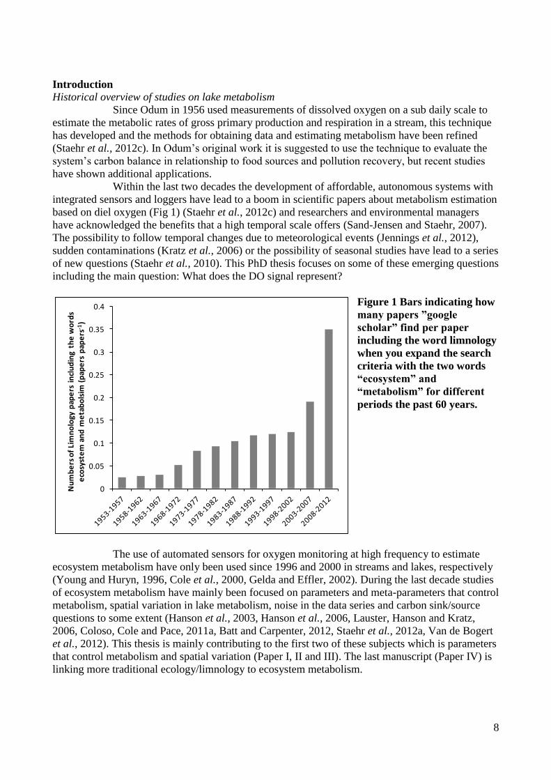
Within the last two decades the development of affordable, autonomous systems with

integrated sensors and loggers have lead to a boom in scientific papers about metabolism estimation

based on diel oxygen (Fig 1) (Staehr et al., 2012c) and researchers and environmental managers

have acknowledged the benefits that a high temporal scale offers (Sand-Jensen and Staehr, 2007).

The possibility to follow temporal changes due to meteorological events (Jennings et al., 2012),

sudden contaminations (Kratz et al., 2006) or the possibility of seasonal studies have lead to a series

of new questions (Staehr et al., 2010). This PhD thesis focuses on some of these emerging questions

including the main question: What does the DO signal represent?

Figure 1 Bars indicating how

many papers ”google

scholar” find per paper

including the word limnology

when you expand the search

criteria with the two words

“ecosystem” and

“metabolism” for different

periods the past 60 years.

The use of automated sensors for oxygen monitoring at high frequency to estimate

ecosystem metabolism have only been used since 1996 and 2000 in streams and lakes, respectively

(Young and Huryn, 1996, Cole et al., 2000, Gelda and Effler, 2002). During the last decade studies

of ecosystem metabolism have mainly been focused on parameters and meta-parameters that control

metabolism, spatial variation in lake metabolism, noise in the data series and carbon sink/source

questions to some extent (Hanson et al., 2003, Hanson et al., 2006, Lauster, Hanson and Kratz,

2006, Coloso, Cole and Pace, 2011a, Batt and Carpenter, 2012, Staehr et al., 2012a, Van de Bogert

et al., 2012). This thesis is mainly contributing to the first two of these subjects which is parameters

that control metabolism and spatial variation (Paper I, II and III). The last manuscript (Paper IV) is

linking more traditional ecology/limnology to ecosystem metabolism.

0

0.05

0.1

0.15

0.2

0.25

0.3

0.35

0.4

Nu

mb

ers

of

Lim

no

logy

pap

ers

in

clu

din

g th

e w

ord

s e

cosy

ste

m a

nd

me

tab

ols

im (

pap

ers

pap

ers

-1)

9

The last decades, whole lake metabolism has been used to evaluate ecosystems as

carbon sinks or sources, or to support food web studies. Also ecosystem response to perturbation

has been widely studied, especially with the introduction of autonomous instrumentation (Kratz et

al., 2006). Many studies have focused on describing the balance between organic matter production

and consumption in the ecosystem. These studies have indicated that most aquatic ecosystems are

net heterotrophic (Net Ecosystem Production (NEP)<0) and hence most receive significant inputs of

organic carbon from adjacent ecosystems (Del Giorgio et al., 1999, Duarte and Prairie, 2005, Cole

et al., 2007, Dodds and Cole, 2007). The studies on whole system carbon balance have inspired

some to study the inland aquatic systems impact on global carbon balance (Cole et al., 2007).

However there are some uncertainties in this analysis which makes it a challenging exercise

associated with a series of assumptions. The greatest potential error is associated with the sampling

bias of the ecosystem. The majority of studied ecosystems are situated in the northern hemisphere,

and are relatively small, natural lakes (Cole et al., 2007). Only a minority of studied lakes are in the

tropics or the arctic (Staehr et al., 2012c). Some studies have also shown that some aquatic

ecosystems can be both CO2 and O2 oversaturated (Christensen, Sand-Jensen and Staehr, 2013),

which complicates the evaluation of the system as a carbon sink or source further.

More recent studies of ecosystem metabolism have been used to identify spatial

location of marked production or degradation of organic matter. This includes studies of the

distribution of production in benthic and pelagic production (Staehr et al., 2012c) or the littoral

compared to pelagic production (Van de Bogert et al., 2007). The latest application of metabolism

studies is the use of sensor derived data as validation for ecosystem models (Prowe et al., 2009,

Staehr et al., 2012c) and future studies will likely integrate ecosystem metabolism and models

further. Through this thesis it is shown that ecosystem metabolism can be used to identify hotspots

of primary production and degradation (papers I and II) and to follow biomass allocation in a

phytoplankton community. In paper IV we quantify the allocation of the carbon that is initially

fixed in the ecosystem and identify the efficiency of different phytoplankton groups in retaining the

fixed carbon as phytoplankton biomass. This knowledge will be useful both for parameterizing of

ecosystem models and in food source studies where it is possible to quantify the proportion of

carbon that is potentially transferred to the next trophic level.

Metabolism in general

Traditionally, metabolism studies have been based on bottle incubations or measurements of

biomass increase measured as chlorophyll a, biovolume or mass, but the relation between these

measurements are associated with a high degree of uncertainty, although theoretically there should

be strong connection between biomass and phytoplankton production (Del Giorgio et al., 1999).

One of the challenges when sampling biomass is the heterogeneity which is much more extreme

than for dissolved substances such as oxygen and CO2. Some of these issues were already

recognized by Wetzel (1965). Even chlorophyll a can be unevenly distributed in lakes (Carrick,

Worth and Marshall, 1994, Borcard et al., 2004, Rinke et al., 2009) and is therefore hard to sample

representatively. Therefore it can be an attractive alternative to measure primary production based

on dissolved products or substrates. There are basically two ways to estimate whole system

metabolism based on pelagic measurements, either by the before-mentioned bottle incubations or by

open water measurements, and within these two approaches there are several ways to measure

metabolism. Metabolism can be estimated from the changes in labeled substrate (e.g. C14

or O18

) or

by total concentration (N) change over time (t) expressed as δN/δt. Many studies have shown that

the different tracers are often comparable in metabolism rates, except for C14

which often

underestimates gross primary production (Bender et al., 1987, Bender et al., 1999, Reeder and

Binion, 2001). Compared to other techniques for metabolism estimation in lakes, which are all

10

based on incubation, the open water technique is essentially different. The open water technique has

some advantages over bottle incubations since it is not affected by “container effects” such as

changed light field, lack of turbulence, fixed depth of the phytoplankton, and sampling issues. Due

to isolation from the environment and the problems of both temporal and spatial scale (Gerhart and

Likens, 1975, Chen, Petersen and Kemp, 2000) bottle incubations are not suitable for extrapolation

and long term studies (Bender et al., 1987). Therefore it has the potential to strengthen predictions

of lake response to changes in environmental conditions on monthly to yearly scale with high

resolution (e.g., climate, deforestation, and eutrophication responses) (Hanson et al., 2006, Kratz et

al., 2006, Tilak et al., 2007, Williamson et al., 2008). This has been demonstrated already in Cole et

al. (2000) where up to four years continuous deployment of sondes are used to analyze net carbon

balance in four different lakes subjected to nutrient addition. As shown in Lauster, Hanson and

Kratz (2006) metabolism estimates based on bottle incubations generally yield lower production

and respiration rates than sonde based measurements, mainly due to significant contribution to the

whole lake metabolism from other parts of a lake, such as benthic primary production or respiration

which may partly be integrated in the sonde measurements. Other locations in a lake that could

potentially contribute to the whole lake metabolism are macrophytes or benthic algae in the littoral

zones, emergent plants, and water-sediment interactions. As shown in Paper I & II, the metalimnion

and hypolimnion of a stratified lake can also contribute significantly to the metabolism rates.

Drawbacks of open water measurements for estimation of metabolic rates include

physical changes in oxygen related to internal waves, mixing, exchange of oxygen with the

atmosphere and chemical processes in the sediment and shore interactions. Finally spatial

patchiness, in the distribution of autotrophs (eg. deep chlorophyll maxima) and heterotrophs make

true whole lake metabolism challenging to evaluate from open water DO measurements (PAPER I).

Seen in this light, it can be an advantage that metabolism estimated from bottle incubations is solely

a pelagic metabolism, while the open water measurements are a combination of pelagic, benthic and

littoral metabolism and may represent some but not all lake metabolism. In addition Wetzel (1965)

noted that the use of oxygen for measurements of production in higher plants might underestimate

production since the plants store oxygen in their tissue (lacunae). Some of these sources of

uncertainties are to a large degree unexplored (Staehr et al., 2010) and therefore there is a demand

for more knowledge on the spatial variation in different lake types.

When estimation of ecosystem metabolism is based on oxygen measurements it is

assumed that the diel oxygen curve is basically a biological signal which results from the balance

between primary production, respiration, and exchange with the atmosphere. The basic principles

for the estimates are, that the change in dissolved oxygen (DO) over time (t) is proportional to net

ecosystem production

, and that NEP is the difference between gross primary

production (GPP) and respiration (R) NEP=GPP-R. It is often assumed that respiration takes place

continuously either at a constant rate, independent of ambient light conditions, or at changing rates

depending on e.g. temperature. GPP is assumed to be dependent on light and can be estimated either

as the sum of NEP and R during light hours or directly as a function of light (I) e.g. GPP=α·I, where

α is the light efficiency coefficient. If the measurements are made in an open system, NEP has to be

corrected for exchange of oxygen with the atmosphere. When NEP < 0 the system is defined as

heterotrophic and when NEP > 0 it is defined as autotrophic (Woodwell and Whittaker, 1968). A

more thorough description of metabolism measures based literature and experiences from this work

follow later.

11

Spatial variation

Historically, the center of the lake has been used as the standard sampling station for

water samples for Winkler titration (e.g. Cloern, Cole and Oremland (1983)), and later also for the

deployment of automated oxygen sensors (Cole et al., 2000, Gelda and Effler, 2002, Staehr and

Sand-Jensen, 2007). It has been the assumption that this location gives the best representation of the

lake or at least the pelagic part, since the littoral zone may behave very differently. Recent studies

have questioned the validity of the metabolic estimates (Staehr and Sand-Jensen, 2007, Van de

Bogert et al., 2007, Hanson et al., 2008) and to what extent the open-water measurements represent

whole-lake metabolism (Lauster et al., 2006, Van de Bogert et al., 2007, Coloso et al., 2008, Sadro,

Melack and MacIntyre, 2011, Van de Bogert et al., 2012). The overall conclusion of these studies

and some of our own preliminary analyses is that one centrally placed sonde yields data that only

reflects the processes in the nearest area, estimated to roughly a 50 m radius in open water and

vertically in the best case most of epilimnion and in some cases only the upper half to one meter of

the epilimnion as concluded in paper II and Coloso, Cole and Pace (2011b).

In stratified lakes, such as many tropical lakes (Kling, 1988), temperate lakes during summer, or

lakes with both saline and freshwater, hypolimnetic oxygen consumption and production are not

measured by a single sonde placed in the upper mixed layer. It has been assumed, that the

production and respiration in hypolimnion is less important due to low rates, a relatively low

volume in many shallow lakes, and that the oxygen deficit in this layer will be registered in the

autumn when the water column is mixed. This assumes that the hypolimnion is completely

separated from the atmosphere during stratification i.e. that there is no reaeration along the edge

from up- or downwelling phenomena. It also requires that oxygen is the only terminal electron

accepter in the hypolimnion, that no gasses escape as bubbles and that production and consumption

in hypolimnion is limited. It also requires that the mixed layer is almost homogeneous at least in the

open waters. However this is often not the case and in these lakes vertical heterogeneity in

metabolism can be expected and are dependent on water clarity and nutrient state (Paper II). GPP

and R have recently been shown to be less dependent on each other than previously anticipated

(Paper II and Solomon et al in press) so while GPP is dependent on the light penetration depth and

the availability of nutrients, respiration is independent of light but can change with depth if the pool

of organic matter changes. Therefore, metabolism estimates from epilimnion alone may in practice

underestimate R and especially GPP in clear lakes (Coloso et al., 2008) though it has often been

assumed that the majority of GPP and R takes place in this layer. To investigate this subject further

we compared vertical variation in metabolism in three contrasting lakes (Paper II) and found as

Sadro et al (2011) that large contributions in both GPP and R from layers below epilimnion can be

expected in clear lakes. This is important because the higher trophic levels in nutrient poor lakes

must be supported by primary production from the whole water column and benthic production if

allochthonous input is limited (Vadeboncoeur, Vander Zanden and Lodge, 2002). Furthermore area

rates of primary production and respiration in clear oligo- and mesotrophic lakes may not be as

different from more eutrophic systems as epilimnetic production alone would indicate

(Vadeboncoeur et al., 2003, Jeppesen et al., 2012) and as we show in paper III, macrophyte

meadows can be very productive, even in very nutrient poor systems. Hence benthic primary

production in shallow parts of oligotrophic lakes can contribute significantly to the system and

support the production of other trophic levels such as bacteria and zooplankton (Vadeboncoeur et

al., 2002). The epilimnion itself can also be heterogeneous in its production pattern, and we found

that a single sonde could give metabolism estimates very far from the depth integrated production in

this layer. Especially in the most eutrophic and hence most turbid lake, significant variations were

observed. This is most likely due to the occurrence of microstratification in the “mixed” layer in

periods of low wind and high temperatures as shown in Coloso et al (2011b). If we look at total area

12

GPP estimates made from single sonde measurements, the conclusion would be that GPP was

increasing with increasing nutrient level, while if we use depth integrated estimates the conclusion

would be the opposite. In the studied ponds of Paper III microstratification was also observed at

depths as low as 25 cm and may be a cause for some of the differences we see between laboratory

and open water measurements.

In order to accommodate issues of horizontal variation in the lakes we made a series

of transects, sailing across one of the studied lakes measuring surface oxygen concentration every

second while logging the position. The data was analyzed using variograms from geostatistics and

showed that the oxygen measurements in the pelagic of a small shallow lake were spatially

autocorrelated within a radius of around 50 meter (data not shown) and that the variation in

measurements was greatest between the littoral zones.

13

Thesis summary

Based on the results from Coloso et al. (2008) we investigated the metabolism and non biological

changes in dissolved oxygen in lakes of different eutrophication status. In Paper I we investigated

lake metabolism in the water column of a clear, stratified lake and found that 1) Metalimnion

contributed significantly to the whole lake metabolism especially when light in adequate amounts

were available at thermocline depth. Metalimnion contributed between 21% and 27% of whole-lake

areal rates of GPP and R respectively when the lake was stratified. 2) Heterotrophy increased with

depth and on average epilimnion was autotrophic while metalimnion was balanced and hypolimnion

was heterotrophic, partly fueled from production excess in overlaying waters. 3) We found that the

DO signal was mainly a result of metabolism and gas exchange with the atmosphere in epilimnion

and cross thermocline fluxes only comprised 10% of the DO variation. In comparison the cross

thermocline fluxes was responsible for half of the DO variation in the metalimnion and almost 80%

in hypolimnion. Most of the fluxes were due to changes in thermocline depth and a test of three

different gas atmosphere exchange models showed no significant difference in the final metabolism

estimates. The fluxes and metabolism analysis was done using data from an automated profiler with

a multiprobe measuring pH, temperature and DO at 30 min intervals at five different depths in the

lake. From these measurements we fitted a model describing temperature profiles in a stratified

lake. We also interpolated oxygen measurements to 1) gain a finer resolution of our measurements

and 2) to smooth out noise in the dataset. The high resolution data was used to estimate the

movement of water and hence oxygen across the thermocline based on equations form Bell et al

(2006). The oxygen changes in each layer excluding the changes due to cross thermocline fluxes

and atmospheric exchange was used to estimate metabolism in each layer. Metabolism was

estimated using a bookkeeping approach on the oxygen profiles, filtered with a moving average of 2

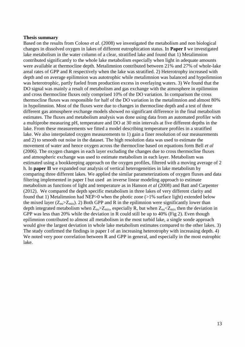
h. In paper II we expanded our analysis of vertical heterogeneities in lake metabolism by

comparing three different lakes. We applied the similar parameterizations of oxygen fluxes and data

filtering implemented in paper I but used an inverse linear modeling approach to estimate

metabolism as functions of light and temperature as in Hanson et al (2008) and Batt and Carpenter

(2012). We compared the depth specific metabolism in three lakes of very different clarity and

found that 1) Metalimnion had NEP>0 when the photic zone (>1% surface light) extended below

the mixed layer (Zeu>Zmix). 2) Both GPP and R in the epilimnion were significantly lower than

depth integrated metabolism when Zeu>Zmix, especially R, but when Zeu<Zmix then the deviation in

GPP was less than 20% while the deviation in R could still be up to 40% (Fig 2). Even though

epilimnion contributed to almost all metabolism in the most turbid lake, a single sonde approach

would give the largest deviation in whole lake metabolism estimates compared to the other lakes. 3)

The study confirmed the findings in paper I of an increasing heterotrophy with increasing depth. 4)

We noted very poor correlation between R and GPP in general, and especially in the most eutrophic

lake.

14

Figure 2 Epilimnetic contribution to whole lake metabolism as a function of the ratio of depth

of euphotic zone (Zeu) and depth of mixed layer (Zmix). Gross primary production (GPP), and

respiration (R) from three lakes of differing trophic state and hence differing clarity (from

Paper II).

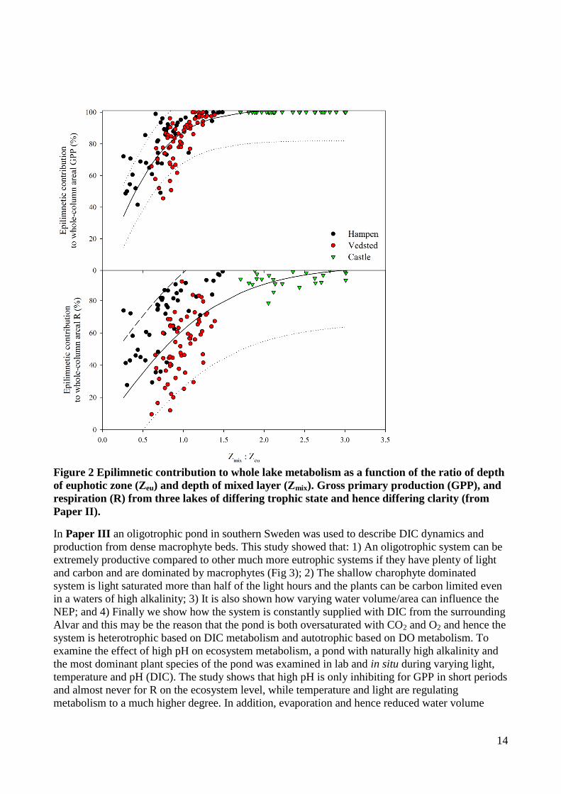
In Paper III an oligotrophic pond in southern Sweden was used to describe DIC dynamics and

production from dense macrophyte beds. This study showed that: 1) An oligotrophic system can be

extremely productive compared to other much more eutrophic systems if they have plenty of light

and carbon and are dominated by macrophytes (Fig 3); 2) The shallow charophyte dominated

system is light saturated more than half of the light hours and the plants can be carbon limited even

in a waters of high alkalinity; 3) It is also shown how varying water volume/area can influence the

NEP; and 4) Finally we show how the system is constantly supplied with DIC from the surrounding

Alvar and this may be the reason that the pond is both oversaturated with CO2 and O2 and hence the

system is heterotrophic based on DIC metabolism and autotrophic based on DO metabolism. To

examine the effect of high pH on ecosystem metabolism, a pond with naturally high alkalinity and

the most dominant plant species of the pond was examined in lab and in situ during varying light,

temperature and pH (DIC). The study shows that high pH is only inhibiting for GPP in short periods

and almost never for R on the ecosystem level, while temperature and light are regulating

metabolism to a much higher degree. In addition, evaporation and hence reduced water volume

15

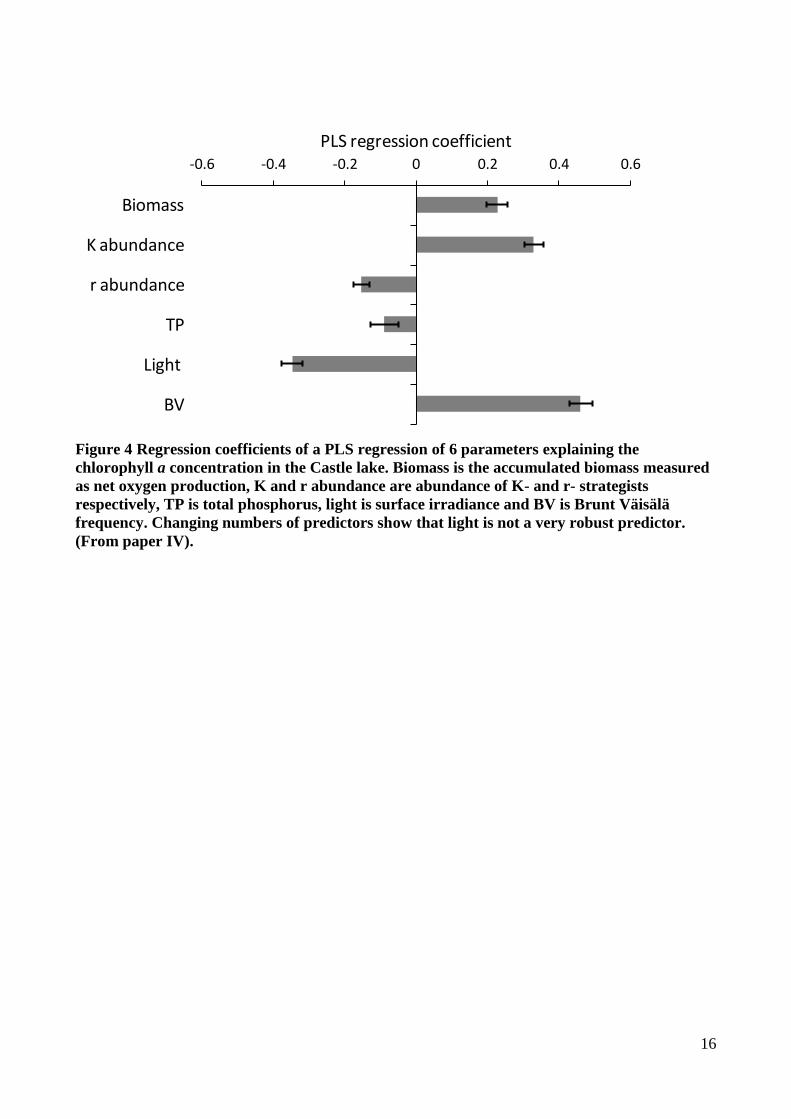
stress the system and force it into net heterotrophy during periods of low water volume. This is

followed by a revitalization of the system during refilling (Fig 3).

Figure 3 Panel A shows the gross primary production (GPP) and respiration (R) of a

Charophyte dominated pond of high alkalinity and panel B shows the net ecosystem

production (NEP) as white bars and maximum depth as a line (From Paper III).

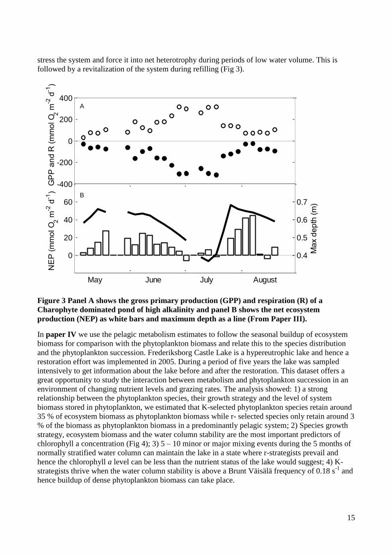
In paper IV we use the pelagic metabolism estimates to follow the seasonal buildup of ecosystem

biomass for comparison with the phytoplankton biomass and relate this to the species distribution

and the phytoplankton succession. Frederiksborg Castle Lake is a hypereutrophic lake and hence a

restoration effort was implemented in 2005. During a period of five years the lake was sampled

intensively to get information about the lake before and after the restoration. This dataset offers a

great opportunity to study the interaction between metabolism and phytoplankton succession in an

environment of changing nutrient levels and grazing rates. The analysis showed: 1) a strong

relationship between the phytoplankton species, their growth strategy and the level of system

biomass stored in phytoplankton, we estimated that K-selected phytoplankton species retain around

35 % of ecosystem biomass as phytoplankton biomass while r- selected species only retain around 3

% of the biomass as phytoplankton biomass in a predominantly pelagic system; 2) Species growth

strategy, ecosystem biomass and the water column stability are the most important predictors of

chlorophyll a concentration (Fig 4); 3) 5 – 10 minor or major mixing events during the 5 months of

normally stratified water column can maintain the lake in a state where r-strategists prevail and

hence the chlorophyll a level can be less than the nutrient status of the lake would suggest; 4) K-

strategists thrive when the water column stability is above a Brunt Väisälä frequency of 0.18 s-1

and

hence buildup of dense phytoplankton biomass can take place.

-400

-200

0

200

400

GP

P a

nd

R (

mm

ol O

2 m

-2 d

-1)

A

0

20

40

60

NE

P (

mm

ol O

2 m

-2 d

-1)

May June July August

B

0.4

0.5

0.6

0.7

Ma

x d

ep

th (

m)

16

Figure 4 Regression coefficients of a PLS regression of 6 parameters explaining the

chlorophyll a concentration in the Castle lake. Biomass is the accumulated biomass measured

as net oxygen production, K and r abundance are abundance of K- and r- strategists

respectively, TP is total phosphorus, light is surface irradiance and BV is Brunt Väisälä

frequency. Changing numbers of predictors show that light is not a very robust predictor.

(From paper IV).

-0.6 -0.4 -0.2 0 0.2 0.4 0.6

Biomass

K abundance

r abundance

TP

Light

BV

PLS regression coefficient

17

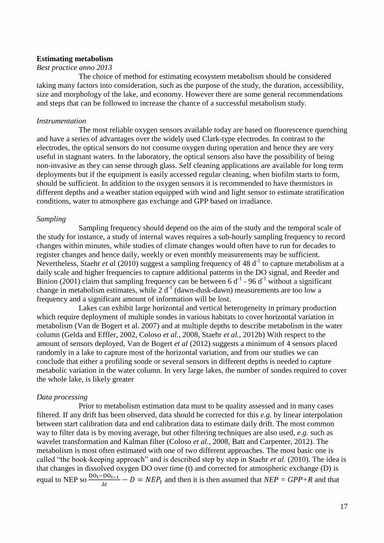
Estimating metabolism

Best practice anno 2013

The choice of method for estimating ecosystem metabolism should be considered

taking many factors into consideration, such as the purpose of the study, the duration, accessibility,

size and morphology of the lake, and economy. However there are some general recommendations

and steps that can be followed to increase the chance of a successful metabolism study.

Instrumentation

The most reliable oxygen sensors available today are based on fluorescence quenching

and have a series of advantages over the widely used Clark-type electrodes. In contrast to the

electrodes, the optical sensors do not consume oxygen during operation and hence they are very

useful in stagnant waters. In the laboratory, the optical sensors also have the possibility of being

non-invasive as they can sense through glass. Self cleaning applications are available for long term

deployments but if the equipment is easily accessed regular cleaning, when biofilm starts to form,

should be sufficient. In addition to the oxygen sensors it is recommended to have thermistors in

different depths and a weather station equipped with wind and light sensor to estimate stratification

conditions, water to atmosphere gas exchange and GPP based on irradiance.

Sampling

Sampling frequency should depend on the aim of the study and the temporal scale of

the study for instance, a study of internal waves requires a sub-hourly sampling frequency to record

changes within minutes, while studies of climate changes would often have to run for decades to

register changes and hence daily, weekly or even monthly measurements may be sufficient.

Nevertheless, Staehr et al (2010) suggest a sampling frequency of 48 d-1

to capture metabolism at a

daily scale and higher frequencies to capture additional patterns in the DO signal, and Reeder and

Binion (2001) claim that sampling frequency can be between 6 d-1

- 96 d-1

without a significant

change in metabolism estimates, while 2 d-1

(dawn-dusk-dawn) measurements are too low a

frequency and a significant amount of information will be lost.

Lakes can exhibit large horizontal and vertical heterogeneity in primary production

which require deployment of multiple sondes in various habitats to cover horizontal variation in

metabolism (Van de Bogert et al. 2007) and at multiple depths to describe metabolism in the water

column (Gelda and Effler, 2002, Coloso et al., 2008, Staehr et al., 2012b) With respect to the

amount of sensors deployed, Van de Bogert et al (2012) suggests a minimum of 4 sensors placed

randomly in a lake to capture most of the horizontal variation, and from our studies we can

conclude that either a profiling sonde or several sensors in different depths is needed to capture

metabolic variation in the water column. In very large lakes, the number of sondes required to cover

the whole lake, is likely greater

Data processing

Prior to metabolism estimation data must to be quality assessed and in many cases

filtered. If any drift has been observed, data should be corrected for this e.g. by linear interpolation

between start calibration data and end calibration data to estimate daily drift. The most common

way to filter data is by moving average, but other filtering techniques are also used, e.g. such as

wavelet transformation and Kalman filter (Coloso et al., 2008, Batt and Carpenter, 2012). The

metabolism is most often estimated with one of two different approaches. The most basic one is

called “the book-keeping approach” and is described step by step in Staehr et al. (2010). The idea is

that changes in dissolved oxygen DO over time (t) and corrected for atmospheric exchange (D) is

equal to NEP so

and then it is then assumed that NEP = GPP+R and that

18

GPP and R are correlated. Most often is it assumed that R during nighttime is equal to daytime R so

daily R can be calculated as average hourly nighttime R times 24, so and

finally GPP can be calculated as GPPday = NEPday + Rday. The other approach can be called “the

inverse modeling approach” and is based on the same basic equations but instead of GPP being

correlated with R, then it is correlated with light (I) e.g. a linear relationship GPP = α · I. The idea

is then to model the DO curve based on the metabolism and gas exchange equations so , where NEP is again the sum GPP and R. Then the parameters of the equation

(α and R) is found by computational iteration techniques were the sum of the difference between the

fitted DO (DOfit) and observed DO (DOobs) is minimized for all observations (n)

(minimize∑ ). Then the optimized parameters can be used to

calculate the metabolism components subsequently.

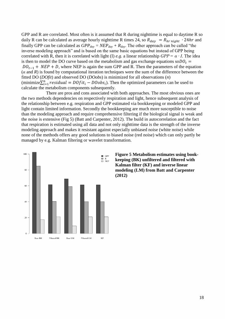
There are pros and cons associated with both approaches. The most obvious ones are

the two methods dependencies on respectively respiration and light, hence subsequent analysis of

the relationship between e.g. respiration and GPP estimated via bookkeeping or modeled GPP and

light contain limited information. Secondly the bookkeeping are much more susceptible to noise

than the modeling approach and require comprehensive filtering if the biological signal is weak and

the noise is extensive (Fig 5) (Batt and Carpenter, 2012). The build in autocorrelation and the fact

that respiration is estimated using all data and not only nighttime data is the strength of the inverse

modeling approach and makes it resistant against especially unbiased noise (white noise) while

none of the methods offers any good solutions to biased noise (red noise) which can only partly be

managed by e.g. Kalman filtering or wavelet transformation.

Figure 5 Metabolism estimates using book-

keeping (BK) unfiltered and filtered with

Kalman filter (KF) and inverse linear

modeling (LM) from Batt and Carpenter

(2012)

19

Conclusions and perspective

This Ph.D. thesis investigated the importance of physical, chemical and biological

conditions on rates of primary production and respiration in a range of small to medium sized lakes.

I document large vertical, spatial variation in lake metabolism and strong relationships dependency

between primary production, phytoplankton biomass and phytoplankton species composition.

Paper I and II are both centered around vertical variation and the main findings

confirm that both primary production and respiration from metalimnion can contribute significantly

to the whole lake metabolism if light is available around the thermocline depth. These results may

have great implications for the interpretation of food sources in especially clear water lakes where

epilimnion primary production is limited. The net balance for a lake may also change significantly

even for eutrophic lakes, if the stratification is persistent and the metalimnion is close to the surface.

The horizontal variation in the pelagic is limited but according to literature the littoral zone can give

significantly different metabolism rates.

It is also shown that nutrient levels in water of macrophyte dominated ponds cannot be

used to predict production very well and carbon may be limiting GPP and likewise in deeper

systems exposed to regular mixing events both chlorophyll a and GPP can be less than predicted

from nutrient status (Paper III and IV).

Future development

Ecosystem metabolism already has a wide range of applications as it is an accounting

for energy entering and leaving the system. Still there are more to come in the future, while this is

still a relatively young discipline within the aquatic sciences. The development in hardware is

probably one of the things that are going to push the development forward while cheaper and more

diverse sensors are being developed. The optical sensor technique offers a great variety in analytes

which makes it possible to combine different metabolism measures such as DIC based metabolism

which is soon made possible with the use of commercial CO2 sensors (Hari et al 2008) or net

growth of phytoplankton biomass with the use of chlorophyll sensors. Cheaper sensors will also

allow an increase in spatial resolution and moving sensor can adjust spatial and temporal resolution

continuously based on the variation in the data already obtained.

On the data processing site a better integration of high frequency data with ecological

models is a likely scenario that both modeling and metabolism studies would benefit from while

models often lack convincing validation for performance and metabolism studies often suffer from

lack in spatial resolution and outlook abilities. Combined with the development of user friendly

software for analysis this could become a strong tool in nature and resource management.

Regarding the estimates of metabolism itself the transfer and integration of methods that strengthen

the predictions of both metabolism rates and derived physiological parameters is essential. The

movement against Baysian methods for parameter estimation and error based filtering technique

like Kalman filter contributes to gain more robust results from field measurements.

Future studies may also involve biodiversity studies since some biodiversity theories

use the total energy input and hence the potential amount of trophic levels to estimate total potential

biodiversity. Wright (1983)(Diane S. Srivastava and John H. Lawton, 1998, Gaston, 2000)

20

References

References

Batt, R.D. & Carpenter, S.R. (2012) Free-water lake metabolism: addressing noisy time series

with a Kalman filter. Limnol. Oceanogr. Methods, 10, 20-30.

Bell, V.A., George, D.G., Moore, R.J. & Parker, J. (2006) Using a 1-D mixing model to

simulate the vertical flux of heat and oxygen in a lake subject to episodic mixing.

Ecological Modelling, 190, 41-54.

Bender, M., Grande, K., Johnson, K., Marra, J., Williams, P., Sieburth, J., Pilson, M.,

Langdon, C., Hitchcock, G. & Orchardo, J. (1987) A comparison of four methods for

determining planktonic community production. Limnol. Oceanogr, 32, 1085-1098.

Bender, M., Orchardo, J., Dickson, M.L., Barber, R. & Lindley, S. (1999) In vitro O2 fluxes

compared with 14

C production and other rate terms during the JGOFS Equatorial

Pacific experiment. Deep-sea research. Part I, Oceanographic research papers, 46, 637-

654.

Borcard, D., Legendre, P., Avois-Jacquet, C. & Tuomisto, H. (2004) Dissecting the spatial

structure of ecological data at multiple scales. Ecology, 85, 1826-1832.

Carrick, H.J., Worth, D. & Marshall, M.L. (1994) The influence of water circulation on

chlorophyll-turbidity relationships in Lake Okeechobee as determined by remote

sensing. Journal of Plankton Research, 16, 1117-1135.

Chen, C.-C., Petersen, J.E. & Kemp, W.M. (2000) Nutrient uptake in experimental estuarine

ecosystems: scaling and partitioning rates. Marine Ecology Progress Series, 200, 103-

116.

Christensen, J.P.A., Sand-Jensen, K. & Staehr, P.A. (2013) Fluctuating water levels control

water chemistry and metabolism of a charophyte dominated pond. Freshwater Biology.

Cloern, J., Cole, B. & Oremland, R. (1983) Seasonal changes in the chemistry and biology of a

meromictic lake (Big Soda Lake, Nevada, U.S.A.). Hydrobiologia, 105, 195-206.

Cole, J., Prairie, Y., Caraco, N., Mcdowell, W., Tranvik, L., Striegl, R., Duarte, C.,

Kortelainen, P., Downing, J., Middelburg, J. & Melack, J. (2007) Plumbing the global

carbon cycle: Integrating inland waters into the terrestrial carbon budget. Ecosystems,

10, 172-185.

Cole, J.J., Pace, M.L., Carpenter, S.R. & Kitchell, J.F. (2000) Persistence of net heterotrophy

in lakes during nutrient addition and food web manipulations. Limnology and

Oceanography, 45, 1718-1730.

Coloso, J., Cole, J. & Pace, M. (2011a) Difficulty in discerning drivers of lake ecosystem

metabolism with high-frequency data. Ecosystems, 14, 935-948.

Coloso, J., Cole, J. & Pace, M. (2011b) Short-term variation in thermal stratification

complicates estimation of lake metabolism. Aquatic Sciences, 73, 305-315.

Coloso, J.J., Cole, J.J., Hanson, P.C. & Pace, M.L. (2008) Depth-integrated, continuous

estimates of metabolism in a clear-water lake. Canadian Journal of Fisheries and

Aquatic Sciences, 65, 712-722.

Del Giorgio, P.A., Cole, J.J., Caraco, N.F. & Peters, R.H. (1999) Linking planktonic biomass

and metabolism to net gas fluxes in northern temperate lakes. Ecology, 80, 1422-1431.

Diane s. srivastava & John h. lawton (1998) Why more productive sites have more species: an

experimental test of theory using tree-hole communities. The American Naturalist, 152,

510-529.

Dodds, W. & Cole, J. (2007) Expanding the concept of trophic state in aquatic ecosystems: it’s

not just the autotrophs. Aquatic Sciences, 69, 427-439.

21

Duarte, C. & Prairie, Y. (2005) Prevalence of heterotrophy and atmospheric CO2 emissions

from aquatic ecosystems. Ecosystems, 8, 862-870.

Gaston, K.J. (2000) Global patterns in biodiversity. Nature, 405, 220-227.

Gelda, R.K. & Effler, S.W. (2002) Metabolic rate estimates for a eutrophic lake from diel

dissolved oxygen signals. Hydrobiologia, 485, 51-66.

Gerhart, D.Z. & Likens, G.E. (1975) Enrichment experiments for determining nutrient

limitation: four methods compared. Limnology and Oceanography, 649-653.

Hanson, P.C., Bade, D.L., Carpenter, S.R. & Kratz, T.K. (2003) Lake metabolism:

relationships with dissolved organic carbon and phosphorus. Limnology and

Oceanography, 48, 1112-1119.

Hanson, P.C., Carpenter, S.R., Armstrong, D.E., Stanley, E.H. & Kratz, T.K. (2006) Lake

dissolved inorganic carbon and dissolved oxygen: changing drivers from days to

decades. Ecological Monographs, 76, 343-363.

Hanson, P.C., Carpenter, S.R., Kimura, N., Wu, C., Cornelius, S.P. & Kratz, T.K. (2008)

Evaluation of metabolism models for free-water dissolved oxygen methods in lakes.

Limnology and Oceanography-Methods, 6, 454-465.

Jennings, E., Jones, S., Arvola, L., Staehr, P.A., Gaiser, E., Jones, I.D., Weathers, K.C.,

Weyhenmeyer, G.A., Chiu, C.-Y. & De Eyto, E. (2012) Effects of weather-related

episodic events in lakes: an analysis based on high-frequency data. Freshwater Biology,

57, 589-601.

Jeppesen, E., Søndergaard, M., Lauridsen, T.L., Davidson, T.A., Liu, Z., Mazzeo, N.,

Trochine, C., Özkan, K., Jensen, H.S., Trolle, D., Starling, F., Lazzaro, X., Johansson,

L.S., Bjerring, R., Liboriussen, L., Larsen, S.E., Landkildehus, F., Egemose, S. &

Meerhoff, M. (2012) Chapter 6 - Biomanipulation as a restoration tool to combat

eutrophication: recent advances and future challenges. In: Advances in Ecological

Research. pp. 411-488. Academic Press.

Kling, G.W. (1988) Comparative transparency, depth of mixing, and stability of stratification

in lakes of Cameroon, West Africa. Limnology and Oceanography, 33, 27-40.

Kratz, T.K., Arzberger, P., Benson, B.J., Chiu, C.-Y., Chiu, K., Ding, L., Fountain, T.,

Hamilton, D., Hanson, P.C. & Hu, Y.H. (2006) Toward a global lake ecological

observatory network. Publications of the Karelian Institute, 145, 51-63.

Lauster, G.H., Hanson, P.C. & Kratz, T.K. (2006) Gross primary production and respiration

differences among littoral and pelagic habitats in northern Wisconsin lakes. Canadian

Journal of Fisheries and Aquatic Sciences, 63, 1130-1141.

Prowe, A.E.F., Thomas, H., Pätsch, J., Kühn, W., Bozec, Y., Schiettecatte, L.-S., Borges, A.V.

& De Baar, H.J.W. (2009) Mechanisms controlling the air–sea flux in the North Sea.

Continental Shelf Research, 29, 1801-1808.

Reeder, B.C. & Binion, B.M. (2001) Comparison of methods to assess water column primary

production in wetlands. Ecological Engineering, 17, 445-449.

Rinke, K., Huber, A.M.R., Kempke, S., Eder, M., Wolf, T., Probst, W.N. & Rothhaupt, K.-O.

(2009) Lake-wide distributions of temperature, phytoplankton, zooplankton, and fish

in the pelagic zone of a large lake. Limnology and Oceanography, 54, 1306-1322.

Sadro, S., Melack, J.M. & Macintyre, S. (2011) Depth-integrated estimates of ecosystem

metabolism in a high-elevation lake (Emerald Lake, Sierra Nevada, California).

Limnol. Oceanogr, 56, 1764-1780.

Sand-Jensen, K. & Staehr, P. (2007) Scaling of pelagic metabolism to size, trophy and forest

cover in small Danish lakes. Ecosystems, 10, 128-142.

22

Staehr, P.A., Baastrup-Spohr, L., Sand-Jensen, K. & Stedmon, C. (2012a) Lake metabolism

scales with lake morphometry and catchment conditions. Aquatic Sciences - Research

Across Boundaries, 74, 155-169.

Staehr, P.A., Bade, D., Van De Bogert, M.C., Koch, G.R., Williamson, C., Hanson, P., Cole,

J.J. & Kratz, T. (2010) Lake metabolism and the diel oxygen technique: State of the

science. Limnology and Oceanography: Methods, 8, 628-644.

Staehr, P.A., Christensen, J.P.A., Batt, R.D. & Read, J.S. (2012b) Ecosystem metabolism in a

stratified lake. Limnol. Oceanogr, 57, 1317-1330.

Staehr, P.A. & Sand-Jensen, K. (2007) Temporal dynamics and regulation of lake

metabolism. Limnology and Oceanography, 52, 108-120.

Staehr, P.A., Testa, J.M., Kemp, W.M., Cole, J.J., Sand-Jensen, K. & Smith, S.V. (2012c) The

metabolism of aquatic ecosystems: history, applications, and future challenges. Aquatic

Sciences-Research Across Boundaries, 74, 15-29.

Tilak, S., Arzberger, P., Balsiger, D., Benson, B., Bhalerao, R., Chiu, K., Fountain, T.,

Hamilton, D., Hanson, P., Kratz, T., Fang Pang, L., Meinke, T. & Winslow, L. (2007)

Conceptual challenges and practical issues in building the Global Lake Ecological

Observatory Network. In: Intelligent Sensors, Sensor Networks and Information, 2007.

ISSNIP 2007. 3rd International Conference on. pp. 721-726.

Vadeboncoeur, Y., Jeppesen, E., Zanden, M.J.V., Schierup, H.-H., Christoffersen, K. &

Lodge, D.M. (2003) From Greenland to green lakes: cultural eutrophication and the

loss of benthic pathways in lakes. Limnology and Oceanography, 48, 1408-1418.

Vadeboncoeur, Y., Vander Zanden, M.J. & Lodge, D.M. (2002) Putting the lake back

together: reintegrating benthic pathways into lake food web models. BioScience, 52,

44-54.

Van De Bogert, M.C., Bade, D.L., Carpenter, S.R., Cole, J.J., Pace, M.L., Hanson, P.C. &

Langman, O.C. (2012) Spatial heterogeneity strongly affects estimates of ecosystem

metabolism in two north temperate lakes. Limnology and Oceanography, 57, 1689.

Van De Bogert, M.C., Carpenter, S.R., Cole, J.J. & Pace, M.L. (2007) Assessing pelagic and

benthic metabolism using free water measurements. Limnol. Oceanogr.: Methods, 5,

145-155.

Wetzel, R.G. (1965) Techniques and problems of primary productivity measurements in

higher aquatic plants and periphyton. In: Primary Productivity in Aquatic

Environments: Proceedings of an IBP PF Symposium. pp. 249. Univ of California Press.

Williamson, C.E., Dodds, W., Kratz, T.K. & Palmer, M.A. (2008) Lakes and streams as

sentinels of environmental change in terrestrial and atmospheric processes. Frontiers

in Ecology and the Environment, 6, 247-254.

Woodwell, G.M. & Whittaker, R.H. (1968) Primary production in terrestrial ecosystems.

American Zoologist, 8, 19-30.

Young, R.G. & Huryn, A.D. (1996) Interannual variation in discharge controls ecosystem

metabolism along a grassland river continuum. Canadian Journal of Fisheries and

Aquatic Sciences, 53, 2199-2211.

23

Paper I

Ecosystem metabolism in a stratified lake

Peter A. Staehr,a,* Jesper P. A. Christensen,b Ryan D. Batt,c and Jordan S. Read d

a Institute of Bioscience, Aarhus University, Roskilde, DenmarkbFreshwater Biological Section, University of Copenhagen, Copenhagen, Denmarkc Center for Limnology, University of Wisconsin–Madison, Madison, WisconsindCivil and Environmental Engineering, University of Wisconsin–Madison, Madison, Wisconsin

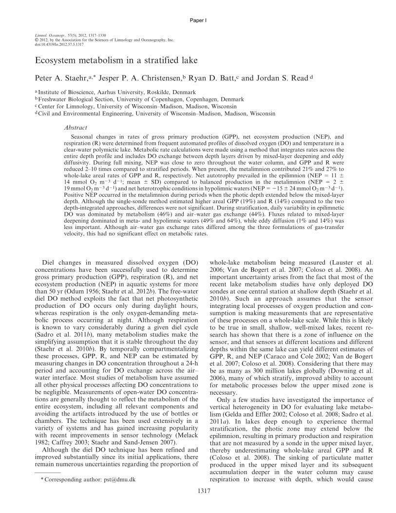
Abstract

Seasonal changes in rates of gross primary production (GPP), net ecosystem production (NEP), andrespiration (R) were determined from frequent automated profiles of dissolved oxygen (DO) and temperature in aclear-water polymictic lake. Metabolic rate calculations were made using a method that integrates rates across theentire depth profile and includes DO exchange between depth layers driven by mixed-layer deepening and eddydiffusivity. During full mixing, NEP was close to zero throughout the water column, and GPP and R werereduced 2–10 times compared to stratified periods. When present, the metalimnion contributed 21% and 27% towhole-lake areal rates of GPP and R, respectively. Net autotrophy prevailed in the epilimnion (NEP 5 11 614 mmol O2 m23 d21; mean 6 SD) compared to balanced production in the metalimnion (NEP 5 2 619 mmol O2 m23 d21) and net heterotrophic conditions in hypolimnic waters (NEP 5 215 6 24 mmol O2 m23 d21).Positive NEP occurred in the metalimnion during periods when the photic depth extended below the mixed-layerdepth. Although the single-sonde method estimated higher areal GPP (19%) and R (14%) compared to the twodepth-integrated approaches, differences were not significant. During stratification, daily variability in epilimneticDO was dominated by metabolism (46%) and air–water gas exchange (44%). Fluxes related to mixed-layerdeepening dominated in meta- and hypolimnic waters (49% and 64%), while eddy diffusion (1% and 14%) wasless important. Although air–water gas exchange rates differed among the three formulations of gas-transfervelocity, this had no significant effect on metabolic rates.

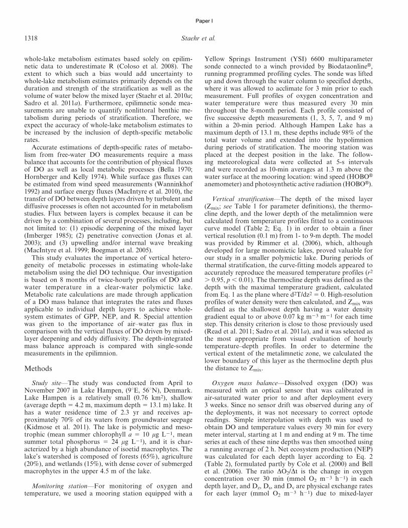
Diel changes in measured dissolved oxygen (DO)concentrations have been successfully used to determinegross primary production (GPP), respiration (R), and netecosystem production (NEP) in aquatic systems for morethan 50 yr (Odum 1956; Staehr et al. 2012b). The free-waterdiel DO method exploits the fact that net photosyntheticproduction of DO occurs only during daylight hours,whereas respiration is the only oxygen-demanding meta-bolic process occurring at night. Although respirationis known to vary considerably during a given diel cycle(Sadro et al. 2011b), many metabolism studies make thesimplifying assumption that it is stable throughout the day(Staehr et al. 2010b). By temporally compartmentalizingthese processes, GPP, R, and NEP can be estimated bymeasuring changes in DO concentration throughout a 24-hperiod and accounting for DO exchange across the air–water interface. Most studies of metabolism have assumedall other physical processes affecting DO concentrations tobe negligible. Measurements of open-water DO concentra-tions are generally thought to reflect the metabolism of theentire ecosystem, including all relevant components andavoiding the artifacts introduced by the use of bottles orchambers. The technique has been used extensively in avariety of systems and has gained increasing popularitywith recent improvements in sensor technology (Melack1982; Caffrey 2003; Staehr and Sand-Jensen 2007).

Although the diel DO technique has been refined andimproved substantially since its initial applications, thereremain numerous uncertainties regarding the proportion of

whole-lake metabolism being measured (Lauster et al.2006; Van de Bogert et al. 2007; Coloso et al. 2008). Animportant uncertainty arises from the fact that most of therecent lake metabolism studies have only deployed DOsondes at one central station at shallow depth (Staehr et al.2010b). Such an approach assumes that the sensorintegrating local processes of oxygen production and con-sumption is making measurements that are representativeof these processes on a whole-lake scale. While this is likelyto be true in small, shallow, well-mixed lakes, recent re-search has shown that there is a zone of influence on thesensor, and that sensors at different locations and differentdepths within the same lake can yield different estimates ofGPP, R, and NEP (Caraco and Cole 2002; Van de Bogertet al. 2007; Coloso et al. 2008). Considering that there maybe as many as 300 million lakes globally (Downing et al.2006), many of which stratify, improved ability to accountfor metabolic processes below the upper mixed zone isnecessary.

Only a few studies have investigated the importance ofvertical heterogeneity in DO for evaluating lake metabo-lism (Gelda and Effler 2002; Coloso et al. 2008; Sadro et al.2011a). In lakes deep enough to experience thermalstratification, the photic zone may extend below theepilimnion, resulting in primary production and respirationthat are not measured by a sonde in the upper mixed layer,thereby underestimating whole-lake areal GPP and R(Coloso et al. 2008). The sinking of particulate matterproduced in the upper mixed layer and its subsequentaccumulation deeper in the water column may causerespiration to increase with depth, which would cause* Corresponding author: pst@dmu.dk

Limnol. Oceanogr., 57(5), 2012, 1317–1330

E 2012, by the Association for the Sciences of Limnology and Oceanography, Inc.doi:10.4319/lo.2012.57.5.1317

1317

Paper I

whole-lake metabolism estimates based solely on epilim-netic data to underestimate R (Coloso et al. 2008). Theextent to which such a bias would add uncertainty towhole-lake metabolism estimates primarily depends on theduration and strength of the stratification as well as thevolume of water below the mixed layer (Staehr et al. 2010a;Sadro et al. 2011a). Furthermore, epilimnetic sonde mea-surements are unable to quantify nonlittoral benthic me-tabolism during periods of stratification. Therefore, weexpect the accuracy of whole-lake metabolism estimates tobe increased by the inclusion of depth-specific metabolicrates.

Accurate estimations of depth-specific rates of metabo-lism from free-water DO measurements require a massbalance that accounts for the contribution of physical fluxesof DO as well as local metabolic processes (Bella 1970;Hornberger and Kelly 1974). While surface gas fluxes canbe estimated from wind speed measurements (Wanninkhof1992) and surface energy fluxes (MacIntyre et al. 2010), thetransfer of DO between depth layers driven by turbulent anddiffusive processes is often not accounted for in metabolismstudies. Flux between layers is complex because it can bedriven by a combination of several processes, including, butnot limited to: (1) episodic deepening of the mixed layer(Imberger 1985); (2) penetrative convection (Jonas et al.2003); and (3) upwelling and/or internal wave breaking(MacIntyre et al. 1999; Boegman et al. 2005).

This study evaluates the importance of vertical hetero-geneity of metabolic processes in estimating whole-lakemetabolism using the diel DO technique. Our investigationis based on 8 months of twice-hourly profiles of DO andwater temperature in a clear-water polymictic lake.Metabolic rate calculations are made through applicationof a DO mass balance that integrates the rates and fluxesapplicable to individual depth layers to achieve whole-system estimates of GPP, NEP, and R. Special attentionwas given to the importance of air–water gas flux incomparison with the vertical fluxes of DO driven by mixed-layer deepening and eddy diffusivity. The depth-integratedmass balance approach is compared with single-sondemeasurements in the epilimnion.

Methods

Study site—The study was conducted from April toNovember 2007 in Lake Hampen, (9uE, 56uN), Denmark.Lake Hampen is a relatively small (0.76 km2), shallow(average depth 5 4.2 m, maximum depth 5 13.1 m) lake. Ithas a water residence time of 2.3 yr and receives ap-proximately 70% of its waters from groundwater seepage(Kidmose et al. 2011). The lake is polymictic and meso-trophic (mean summer chlorophyll a 5 10 mg L21, meansummer total phosphorus 5 24 mg L21), and it is char-acterized by a high abundance of isoetid macrophytes. Thelake’s watershed is composed of forests (65%), agriculture(20%), and wetlands (15%), with dense cover of submergedmacrophytes in the upper 4.5 m of the lake.

Monitoring station—For monitoring of oxygen andtemperature, we used a mooring station equipped with a

Yellow Springs Instrument (YSI) 6600 multiparametersonde connected to a winch provided by BiodataonlineH,running programmed profiling cycles. The sonde was liftedup and down through the water column to specified depths,where it was allowed to acclimate for 3 min prior to eachmeasurement. Full profiles of oxygen concentration andwater temperature were thus measured every 30 minthroughout the 8-month period. Each profile consisted offive successive depth measurements (1, 3, 5, 7, and 9 m)within a 20-min period. Although Hampen Lake has amaximum depth of 13.1 m, these depths include 98% of thetotal water volume and extended into the hypolimnionduring periods of stratification. The mooring station wasplaced at the deepest position in the lake. The follow-ing meteorological data were collected at 5-s intervalsand were recorded as 10-min averages at 1.3 m above thewater surface at the mooring location: wind speed (HOBOHanemometer) and photosynthetic active radiation (HOBOH).

Vertical stratification—The depth of the mixed layer(Zmix; see Table 1 for parameter definitions), the thermo-cline depth, and the lower depth of the metalimnion werecalculated from temperature profiles fitted to a continuouscurve model (Table 2; Eq. 1) in order to obtain a finervertical resolution (0.1 m) from 1- to 9-m depth. The modelwas provided by Rimmer et al. (2006), which, althoughdeveloped for large monomictic lakes, proved valuable forour study in a smaller polymictic lake. During periods ofthermal stratification, the curve-fitting models appeared toaccurately reproduce the measured temperature profiles (r2

. 0.95, p , 0.01). The thermocline depth was defined as thedepth with the maximal temperature gradient, calculatedfrom Eq. 1 as the plane where d2T/dz2 5 0. High-resolutionprofiles of water density were then calculated, and Zmix wasdefined as the shallowest depth having a water densitygradient equal to or above 0.07 kg m23 m21 for each timestep. This density criterion is close to those previously used(Read et al. 2011; Sadro et al. 2011a), and it was selected asthe most appropriate from visual evaluation of hourlytemperature–depth profiles. In order to determine thevertical extent of the metalimnetic zone, we calculated thelower boundary of this layer as the thermocline depth plusthe distance to Zmix.

Oxygen mass balance—Dissolved oxygen (DO) wasmeasured with an optical sensor that was calibrated inair-saturated water prior to and after deployment every3 weeks. Since no sensor drift was observed during any ofthe deployments, it was not necessary to correct optodereadings. Simple interpolation with depth was used toobtain DO and temperature values every 30 min for everymeter interval, starting at 1 m and ending at 9 m. The timeseries at each of these nine depths was then smoothed usinga running average of 2 h. Net ecosystem production (NEP)was calculated for each depth layer according to Eq. 2(Table 2), formulated partly by Cole et al. (2000) and Bellet al. (2006). The ratio DO2/Dt is the change in oxygenconcentration over 30 min (mmol O2 m23 h21) in eachdepth layer, and Dz, Ds, and Dv are physical exchange ratesfor each layer (mmol O2 m23 h21) due to mixed-layer

1318 Staehr et al.

Paper I

deepening, diffusive gas exchange with the atmosphere, andeddy diffusivity (Table 2, Eq. 8–10). Ds was only applied tomeasurements above Zmix, as the remaining layers wereconsidered to be isolated from the atmosphere (see Fig. 1).Above Zmix, diffusion (Ds) into layer i was calculated asDs(i) 5 Ks(O2(i) 2 O2sat)/Zmix (Table 2; Eq. 9), where O2sat

is the concentration of oxygen in equilibrium with theatmosphere, O2(i) is the measured concentration of oxy-gen in layer I, and Ks is the coefficient of gas exchange of

oxygen at a given temperature. The value of k600 (k for aSchmidt number of 600) was calculated from wind speed(MacIntyre et al. 2010) using different equations undercooling and heating conditions (Table 2; Eq. 6a,b). In orderto investigate the importance of different formulations ofk600, we also evaluated a wind-driven formulation by Coleand Caraco (1998) and Crusius and Wanninkhof (2003)(Table 2; Eq. 6c,d). Assuming a neutrally stable boundarylayer, wind speed at 10 m was calculated using the empirical

Table 1. Definition of parameters used to model lake metabolism.

Parameter Definition

O2sat Concentration of DO at 100% saturation for any given temperature (mmol O2 m23)O2 Concentration of DO (mmol O2 m23)DO2/Dt Change in DO per hour (mmol O2 m23 h21)GPP Gross primary production (mmol O2 m23 h21)NEP Net ecosystem production (mmol O2 m23 h21)PAZ Areal proportion of each depth strataR Lake respiration (mmol O2 m23 h21)D Diffusion rate (mmol O2 m23 h21)K600 Gas-transfer velocity normalized to Schmidts number of 600Ks Gas exchange rate with atmosphere (cm h21)Kv Vertical turbulent diffusivity (m2 h21)Sc Schmidt numbern Temperature curve fitting parameter (dimensionless)A Temperature curve fitting parameter (m21)N2 Brunt-Vaisala buoyancy frequency (s22)r Water density (kg m23)Te and Th Maximum temperature in epilimnion and minimum in hypolimnion (uC)U10 Wind speed in 10 m height (m s21)A Area of the lake (m22) at surface or at depth iVi Volume of layer i or of the epilimnion (epi) (m23)h Height of the depth layers (0.5 m)Z or Zi Depth or depth of layer i (m)Zmix Mixing depth (m)Zeu Photic zone depth (m) corresponding to 1% of surface light

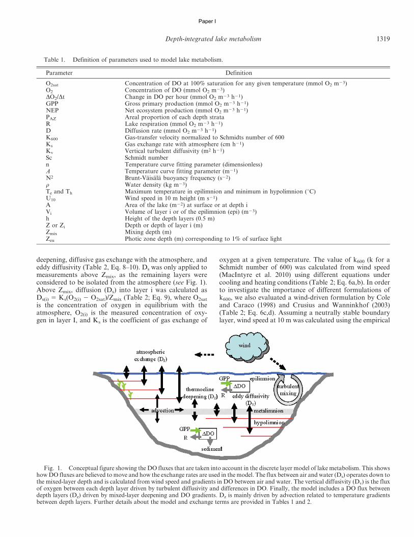
Fig. 1. Conceptual figure showing the DO fluxes that are taken into account in the discrete layer model of lake metabolism. This showshow DO fluxes are believed to move and how the exchange rates are used in the model. The flux between air and water (Ds) operates down tothe mixed-layer depth and is calculated from wind speed and gradients in DO between air and water. The vertical diffusivity (Dv) is the fluxof oxygen between each depth layer driven by turbulent diffusivity and differences in DO. Finally, the model includes a DO flux betweendepth layers (Dz) driven by mixed-layer deepening and DO gradients. Dz is mainly driven by advection related to temperature gradientsbetween depth layers. Further details about the model and exchange terms are provided in Tables 1 and 2.

Depth-integrated lake metabolism 1319

Paper I

relationship described in Smith (1985) from wind speedmeasurements made at the center of the lake, 1.3 m abovethe surface. The coefficient of oxygen exchange (Ks) wascalculated every 30 min from the estimate of k600 and theratio of Schmidt numbers according to Jahne et al. (1987)(Table 2; Eq. 7).

Exchange of oxygen between adjacent depth layerscaused by turbulent diffusivity (Dv) was calculated fromthe vertical eddy diffusivity coefficient (Kv, m2 h21), whichis used here to approximate the movement of oxygenbetween adjacent depth layers (Table 2; Eq. 3). Negativevalues of Dv are fluxes into and positive values are fluxesout of a given depth stratum. Mixing of epilimnetic andhypolimnetic water caused by changes in mixed-layer depthduring stratification was accounted for by subtracting Dz

from NEP calculations (Table 2; Eq. 2) (see Fig. 1)according to the methods of Bell et al. (2006). Dz dependson the deepening rate of the mixing depth and the relativeconcentrations of adjacent layers. The deepening rate(DZmix/Dt; m h21) describes the velocity of the mixed-layerdeepening in both directions; it is positive when the volumeof the hypolimnion is decreasing and negative when thehypolimnetic volume is increasing. By dividing the deep-ening rate by the height of discrete layers (1 m)

and multiplying by the DO gradient between two adjacentlayers, we can calculate the flux of DO due to mixed-layerdeepening (Dz; Table 2; Eq. 10).

Having obtained NEP rates for 30-min intervals in allnine depth layers, we calculated daily values of gross pri-mary production (GPP; mmol O2 m23 d21) and ecosystemrespiration (R; mmol O2 m23 d21) for each depth layer.Because there is no GPP at night, we assumed that night-time R equals nighttime NEP. While we cannot directlymeasure R during the day, if we assume that the daytimerate of R is equal to that of nighttime R (Cole et al. 2000;Hanson et al. 2003; Lauster et al. 2006), daily R equalsRnight (h21) times 24 h (Table 2; Eq.11). Hourly nighttimerespiration rates were calculated from changes in oxygenduring darkness, after excluding 1-h periods just beforesunrise and just after sunset. Knowing NEP and R ratesallowed us to estimate GPP by adding daytime NEP to R(Staehr et al. 2010b) (Table 2; Eq. 12). It is likely thatdaytime R exceeds nighttime R (Pace and Prairie 2005;Tobias et al. 2007), which would result in the magnitudes ofGPP and R being underestimated, but this would not havean effect on NEP since this is a result of the balance of GPPand R (Cole et al. 2000). For each depth layer, the met-abolic balance between GPP and R on a daily basis was

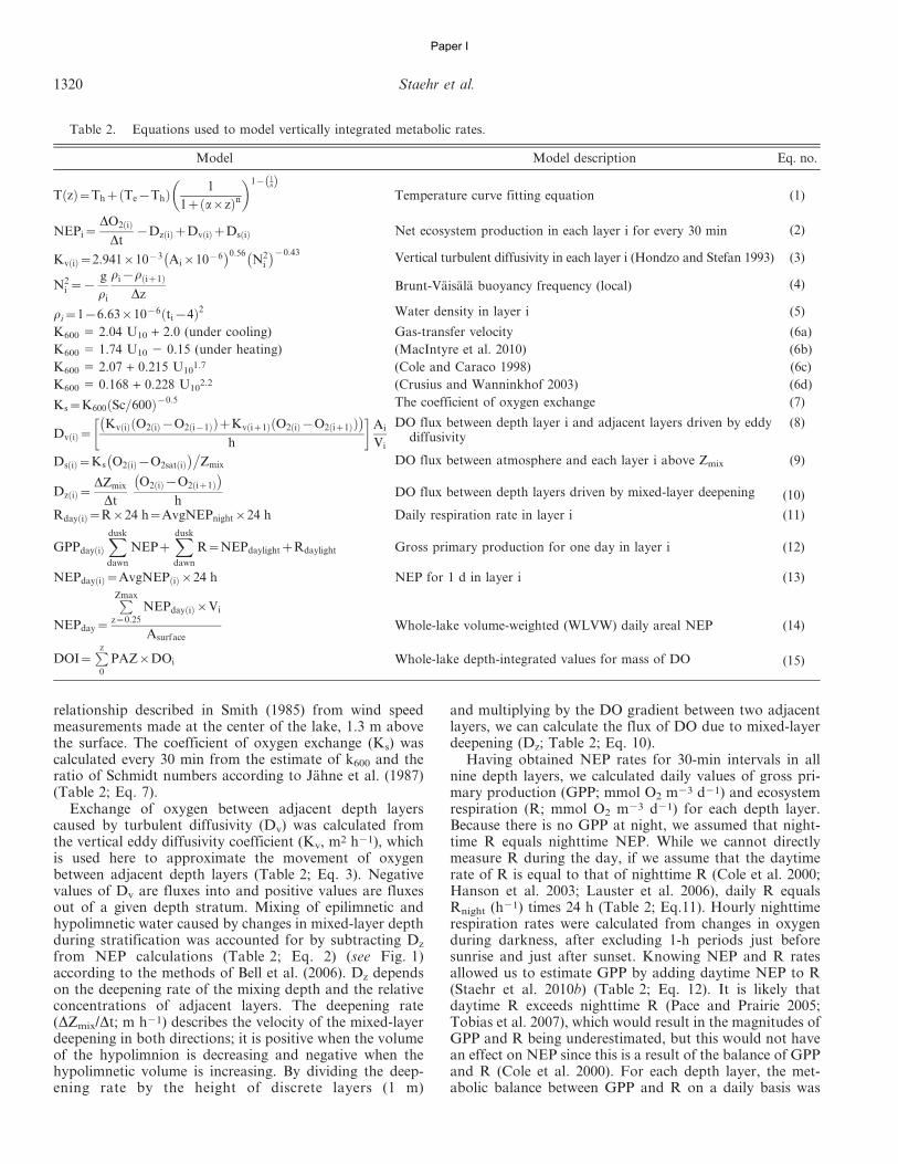
Table 2. Equations used to model vertically integrated metabolic rates.

Model Model description Eq. no.

T zð Þ~Thz Te{Thð Þ 1

1z a|zð Þn� �1{ 1

nð ÞTemperature curve fitting equation (1)

NEPi~DO2 ið ÞDt

{Dz ið ÞzDv ið ÞzDs ið Þ Net ecosystem production in each layer i for every 30 min (2)

Kv ið Þ~2:941|10{3 Ai|10{6� �0:56

N2i

� �{0:43Vertical turbulent diffusivity in each layer i (Hondzo and Stefan 1993) (3)

N2i ~{

g

ri

ri{r iz1ð ÞDz

Brunt-Vaisala buoyancy frequency (local) (4)

ri~1{6:63|10{6 ti{4ð Þ2 Water density in layer i (5)

K600 5 2.04 U10 + 2.0 (under cooling) Gas-transfer velocity (6a)

K600 5 1.74 U10 2 0.15 (under heating) (MacIntyre et al. 2010) (6b)

K600 5 2.07 + 0.215 U101.7 (Cole and Caraco 1998) (6c)

K600 5 0.168 + 0.228 U102.2 (Crusius and Wanninkhof 2003) (6d)

Ks~K600 Sc=600ð Þ{0:5 The coefficient of oxygen exchange (7)

Dv ið Þ~Kv ið ÞðO2 ið Þ{O2 i{1ð ÞÞzKv iz1ð ÞðO2 ið Þ{O2 iz1ð ÞÞ� �

h

� �Ai

Vi

DO flux between depth layer i and adjacent layers driven by eddydiffusivity

(8)

Ds ið Þ~Ks O2 ið Þ{O2sat ið Þ� ��

Zmix DO flux between atmosphere and each layer i above Zmix (9)

Dz ið Þ~DZmix

Dt

O2 ið Þ{O2 iz1ð Þ� �

hDO flux between depth layers driven by mixed-layer deepening (10)

Rday ið Þ~R|24 h~AvgNEPnight|24 h Daily respiration rate in layer i (11)

GPPday ið ÞXdusk

dawn

NEPzXdusk

dawn

R~NEPdaylightzRdaylight Gross primary production for one day in layer i (12)

NEPday ið Þ~AvgNEP ið Þ|24 h NEP for 1 d in layer i (13)

NEPday~

PZmax

z~0:25

NEPday ið Þ|Vi

AsurfaceWhole-lake volume-weighted (WLVW) daily areal NEP (14)

DOI~Pz0

PAZ|DOi Whole-lake depth-integrated values for mass of DO (15)

1320 Staehr et al.

Paper I

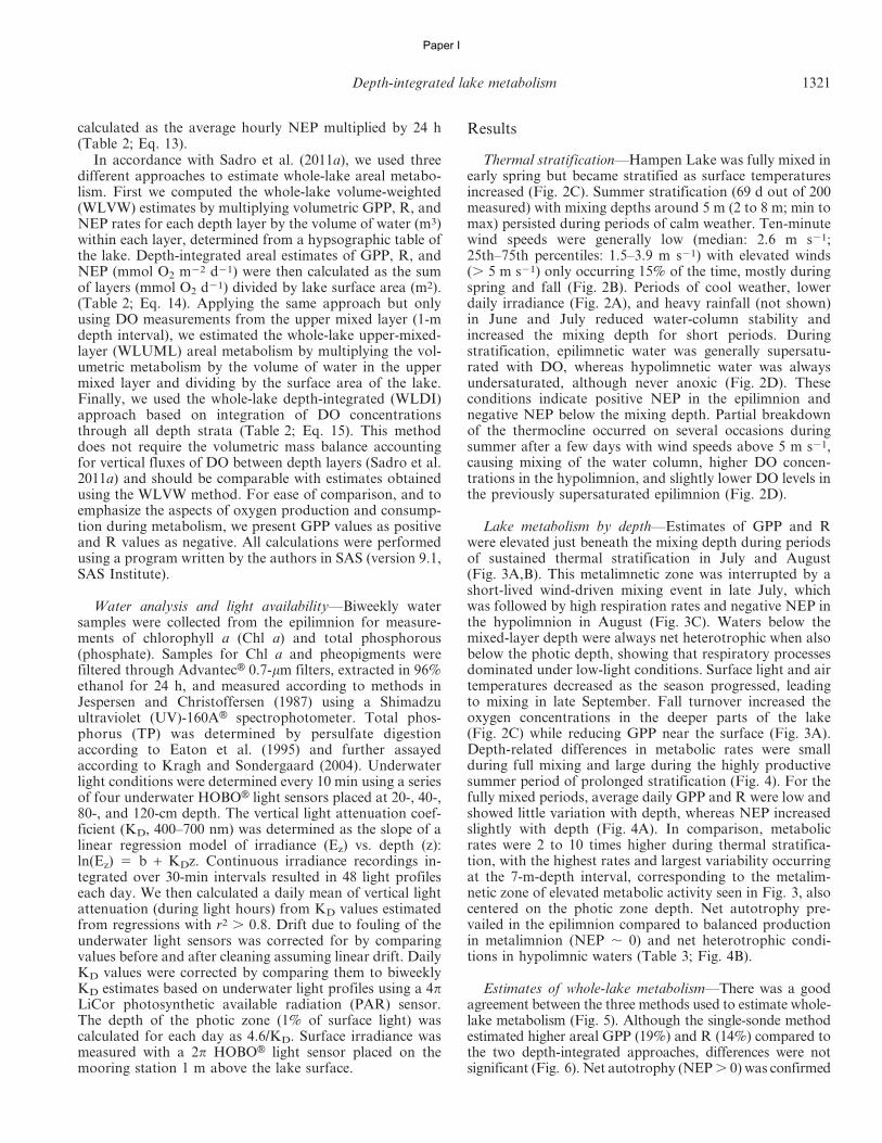
calculated as the average hourly NEP multiplied by 24 h(Table 2; Eq. 13).

In accordance with Sadro et al. (2011a), we used threedifferent approaches to estimate whole-lake areal metabo-lism. First we computed the whole-lake volume-weighted(WLVW) estimates by multiplying volumetric GPP, R, andNEP rates for each depth layer by the volume of water (m3)within each layer, determined from a hypsographic table ofthe lake. Depth-integrated areal estimates of GPP, R, andNEP (mmol O2 m22 d21) were then calculated as the sumof layers (mmol O2 d21) divided by lake surface area (m2).(Table 2; Eq. 14). Applying the same approach but onlyusing DO measurements from the upper mixed layer (1-mdepth interval), we estimated the whole-lake upper-mixed-layer (WLUML) areal metabolism by multiplying the vol-umetric metabolism by the volume of water in the uppermixed layer and dividing by the surface area of the lake.Finally, we used the whole-lake depth-integrated (WLDI)approach based on integration of DO concentrationsthrough all depth strata (Table 2; Eq. 15). This methoddoes not require the volumetric mass balance accountingfor vertical fluxes of DO between depth layers (Sadro et al.2011a) and should be comparable with estimates obtainedusing the WLVW method. For ease of comparison, and toemphasize the aspects of oxygen production and consump-tion during metabolism, we present GPP values as positiveand R values as negative. All calculations were performedusing a program written by the authors in SAS (version 9.1,SAS Institute).

Water analysis and light availability—Biweekly watersamples were collected from the epilimnion for measure-ments of chlorophyll a (Chl a) and total phosphorous(phosphate). Samples for Chl a and pheopigments werefiltered through AdvantecH 0.7-mm filters, extracted in 96%ethanol for 24 h, and measured according to methods inJespersen and Christoffersen (1987) using a Shimadzuultraviolet (UV)-160AH spectrophotometer. Total phos-phorus (TP) was determined by persulfate digestionaccording to Eaton et al. (1995) and further assayedaccording to Kragh and Sondergaard (2004). Underwaterlight conditions were determined every 10 min using a seriesof four underwater HOBOH light sensors placed at 20-, 40-,80-, and 120-cm depth. The vertical light attenuation coef-ficient (KD, 400–700 nm) was determined as the slope of alinear regression model of irradiance (Ez) vs. depth (z):ln(Ez) 5 b + KDz. Continuous irradiance recordings in-tegrated over 30-min intervals resulted in 48 light profileseach day. We then calculated a daily mean of vertical lightattenuation (during light hours) from KD values estimatedfrom regressions with r2 . 0.8. Drift due to fouling of theunderwater light sensors was corrected for by comparingvalues before and after cleaning assuming linear drift. DailyKD values were corrected by comparing them to biweeklyKD estimates based on underwater light profiles using a 4pLiCor photosynthetic available radiation (PAR) sensor.The depth of the photic zone (1% of surface light) wascalculated for each day as 4.6/KD. Surface irradiance wasmeasured with a 2p HOBOH light sensor placed on themooring station 1 m above the lake surface.

Results

Thermal stratification—Hampen Lake was fully mixed inearly spring but became stratified as surface temperaturesincreased (Fig. 2C). Summer stratification (69 d out of 200measured) with mixing depths around 5 m (2 to 8 m; min tomax) persisted during periods of calm weather. Ten-minutewind speeds were generally low (median: 2.6 m s21;25th–75th percentiles: 1.5–3.9 m s21) with elevated winds(. 5 m s21) only occurring 15% of the time, mostly duringspring and fall (Fig. 2B). Periods of cool weather, lowerdaily irradiance (Fig. 2A), and heavy rainfall (not shown)in June and July reduced water-column stability andincreased the mixing depth for short periods. Duringstratification, epilimnetic water was generally supersatu-rated with DO, whereas hypolimnetic water was alwaysundersaturated, although never anoxic (Fig. 2D). Theseconditions indicate positive NEP in the epilimnion andnegative NEP below the mixing depth. Partial breakdownof the thermocline occurred on several occasions duringsummer after a few days with wind speeds above 5 m s21,causing mixing of the water column, higher DO concen-trations in the hypolimnion, and slightly lower DO levels inthe previously supersaturated epilimnion (Fig. 2D).

Lake metabolism by depth—Estimates of GPP and Rwere elevated just beneath the mixing depth during periodsof sustained thermal stratification in July and August(Fig. 3A,B). This metalimnetic zone was interrupted by ashort-lived wind-driven mixing event in late July, whichwas followed by high respiration rates and negative NEP inthe hypolimnion in August (Fig. 3C). Waters below themixed-layer depth were always net heterotrophic when alsobelow the photic depth, showing that respiratory processesdominated under low-light conditions. Surface light and airtemperatures decreased as the season progressed, leadingto mixing in late September. Fall turnover increased theoxygen concentrations in the deeper parts of the lake(Fig. 2C) while reducing GPP near the surface (Fig. 3A).Depth-related differences in metabolic rates were smallduring full mixing and large during the highly productivesummer period of prolonged stratification (Fig. 4). For thefully mixed periods, average daily GPP and R were low andshowed little variation with depth, whereas NEP increasedslightly with depth (Fig. 4A). In comparison, metabolicrates were 2 to 10 times higher during thermal stratifica-tion, with the highest rates and largest variability occurringat the 7-m-depth interval, corresponding to the metalim-netic zone of elevated metabolic activity seen in Fig. 3, alsocentered on the photic zone depth. Net autotrophy pre-vailed in the epilimnion compared to balanced productionin metalimnion (NEP , 0) and net heterotrophic condi-tions in hypolimnic waters (Table 3; Fig. 4B).

Estimates of whole-lake metabolism—There was a goodagreement between the three methods used to estimate whole-lake metabolism (Fig. 5). Although the single-sonde methodestimated higher areal GPP (19%) and R (14%) compared tothe two depth-integrated approaches, differences were notsignificant (Fig. 6). Net autotrophy (NEP . 0) was confirmed

Depth-integrated lake metabolism 1321

Paper I

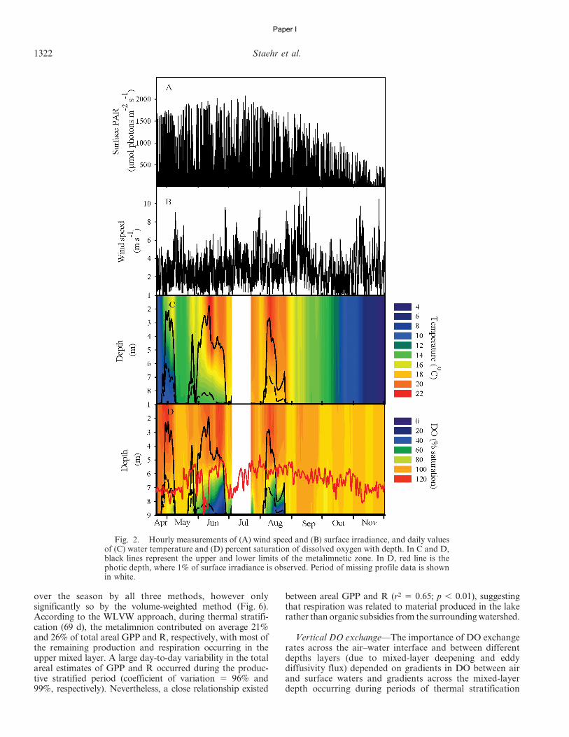
over the season by all three methods, however onlysignificantly so by the volume-weighted method (Fig. 6).According to the WLVW approach, during thermal stratifi-cation (69 d), the metalimnion contributed on average 21%and 26% of total areal GPP and R, respectively, with most ofthe remaining production and respiration occurring in theupper mixed layer. A large day-to-day variability in the totalareal estimates of GPP and R occurred during the produc-tive stratified period (coefficient of variation 5 96% and99%, respectively). Nevertheless, a close relationship existed

between areal GPP and R (r2 5 0.65; p , 0.01), suggestingthat respiration was related to material produced in the lakerather than organic subsidies from the surrounding watershed.

Vertical DO exchange—The importance of DO exchangerates across the air–water interface and between differentdepths layers (due to mixed-layer deepening and eddydiffusivity flux) depended on gradients in DO between airand surface waters and gradients across the mixed-layerdepth occurring during periods of thermal stratification

Fig. 2. Hourly measurements of (A) wind speed and (B) surface irradiance, and daily valuesof (C) water temperature and (D) percent saturation of dissolved oxygen with depth. In C and D,black lines represent the upper and lower limits of the metalimnetic zone. In D, red line is thephotic depth, where 1% of surface irradiance is observed. Period of missing profile data is shownin white.

1322 Staehr et al.

Paper I

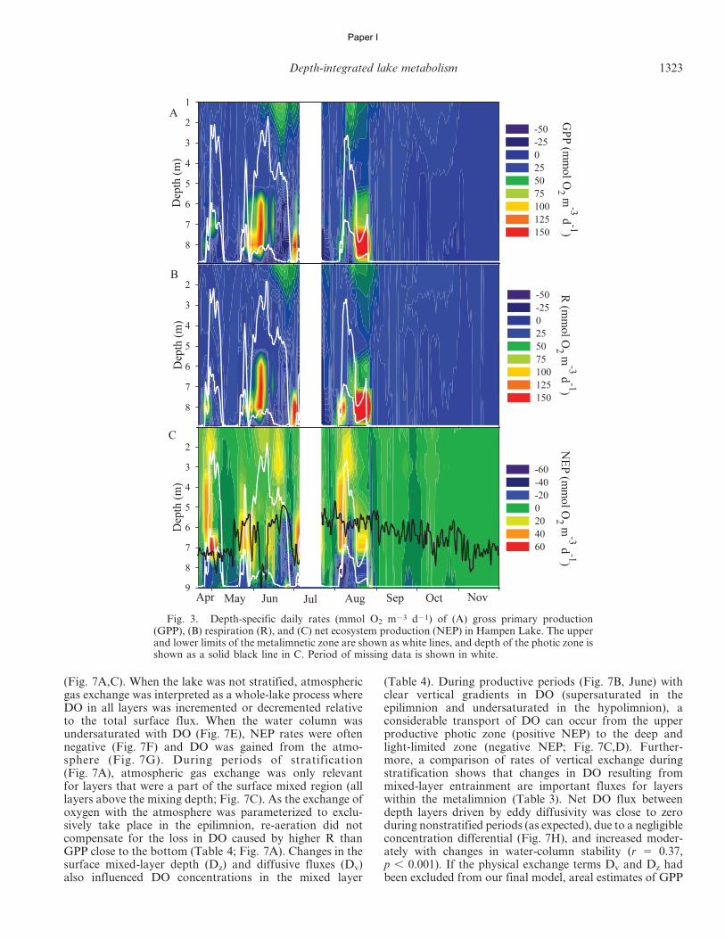
(Fig. 7A,C). When the lake was not stratified, atmosphericgas exchange was interpreted as a whole-lake process whereDO in all layers was incremented or decremented relativeto the total surface flux. When the water column wasundersaturated with DO (Fig. 7E), NEP rates were oftennegative (Fig. 7F) and DO was gained from the atmo-sphere (Fig. 7G). During periods of stratification(Fig. 7A), atmospheric gas exchange was only relevantfor layers that were a part of the surface mixed region (alllayers above the mixing depth; Fig. 7C). As the exchange ofoxygen with the atmosphere was parameterized to exclu-sively take place in the epilimnion, re-aeration did notcompensate for the loss in DO caused by higher R thanGPP close to the bottom (Table 4; Fig. 7A). Changes in thesurface mixed-layer depth (Dz) and diffusive fluxes (Dv)also influenced DO concentrations in the mixed layer

(Table 4). During productive periods (Fig. 7B, June) withclear vertical gradients in DO (supersaturated in theepilimnion and undersaturated in the hypolimnion), aconsiderable transport of DO can occur from the upperproductive photic zone (positive NEP) to the deep andlight-limited zone (negative NEP; Fig. 7C,D). Further-more, a comparison of rates of vertical exchange duringstratification shows that changes in DO resulting frommixed-layer entrainment are important fluxes for layerswithin the metalimnion (Table 3). Net DO flux betweendepth layers driven by eddy diffusivity was close to zeroduring nonstratified periods (as expected), due to a negligibleconcentration differential (Fig. 7H), and increased moder-ately with changes in water-column stability (r 5 0.37,p , 0.001). If the physical exchange terms Dv and Dz hadbeen excluded from our final model, areal estimates of GPP

Fig. 3. Depth-specific daily rates (mmol O2 m23 d21) of (A) gross primary production(GPP), (B) respiration (R), and (C) net ecosystem production (NEP) in Hampen Lake. The upperand lower limits of the metalimnetic zone are shown as white lines, and depth of the photic zone isshown as a solid black line in C. Period of missing data is shown in white.

Depth-integrated lake metabolism 1323

Paper I

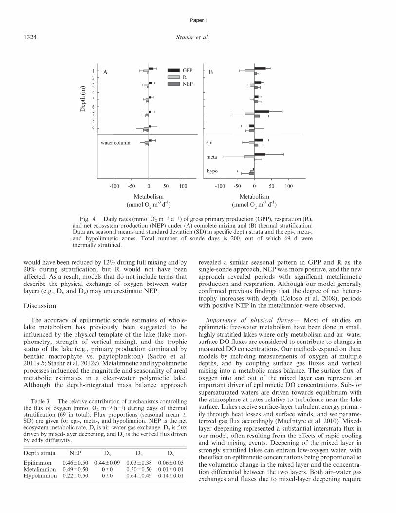
would have been reduced by 12% during full mixing and by20% during stratification, but R would not have beenaffected. As a result, models that do not include terms thatdescribe the physical exchange of oxygen between waterlayers (e.g., Dv and Dz) may underestimate NEP.

Discussion

The accuracy of epilimnetic sonde estimates of whole-lake metabolism has previously been suggested to beinfluenced by the physical template of the lake (lake mor-phometry, strength of vertical mixing), and the trophicstatus of the lake (e.g., primary production dominated bybenthic macrophyte vs. phytoplankton) (Sadro et al.2011a,b; Staehr et al. 2012a). Metalimnetic and hypolimneticprocesses influenced the magnitude and seasonality of arealmetabolic estimates in a clear-water polymictic lake.Although the depth-integrated mass balance approach

revealed a similar seasonal pattern in GPP and R as thesingle-sonde approach, NEP was more positive, and the newapproach revealed periods with significant metalimneticproduction and respiration. Although our model generallyconfirmed previous findings that the degree of net hetero-trophy increases with depth (Coloso et al. 2008), periodswith positive NEP in the metalimnion were observed.

Importance of physical fluxes— Most of studies onepilimnetic free-water metabolism have been done in small,highly stratified lakes where only metabolism and air–watersurface DO fluxes are considered to contribute to changes inmeasured DO concentrations. Our methods expand on thesemodels by including measurements of oxygen at multipledepths, and by coupling surface gas fluxes and verticalmixing into a metabolic mass balance. The surface flux ofoxygen into and out of the mixed layer can represent animportant driver of epilimnetic DO concentrations. Sub- orsupersaturated waters are driven towards equilibrium withthe atmosphere at rates relative to turbulence near the lakesurface. Lakes receive surface-layer turbulent energy primar-ily through heat losses and surface winds, and we parame-terized gas flux accordingly (MacIntyre et al. 2010). Mixed-layer deepening represented a substantial interstrata flux inour model, often resulting from the effects of rapid coolingand wind mixing events. Deepening of the mixed layer instrongly stratified lakes can entrain low-oxygen water, withthe effect on epilimnetic concentrations being proportional tothe volumetric change in the mixed layer and the concentra-tion differential between the two layers. Both air–water gasexchanges and fluxes due to mixed-layer deepening require

Fig. 4. Daily rates (mmol O2 m23 d21) of gross primary production (GPP), respiration (R),and net ecosystem production (NEP) under (A) complete mixing and (B) thermal stratification.Data are seasonal means and standard deviation (SD) in specific depth strata and the epi-, meta-,and hypolimnetic zones. Total number of sonde days is 200, out of which 69 d werethermally stratified.

Table 3. The relative contribution of mechanisms controllingthe flux of oxygen (mmol O2 m23 h21) during days of thermalstratification (69 in total). Flux proportions (seasonal mean 6SD) are given for epi-, meta-, and hypolimnion. NEP is the netecosystem metabolic rate, Ds is air–water gas exchange, Dz is fluxdriven by mixed-layer deepening, and Dv is the vertical flux drivenby eddy diffusivity.

Depth strata NEP Ds Dz Dv

Epilimnion 0.4660.50 0.4460.09 0.0360.38 0.0660.03Metalimnion 0.4960.50 060 0.5060.50 0.0160.01Hypolimnion 0.2260.50 060 0.6460.49 0.1460.01

1324 Staehr et al.

Paper I

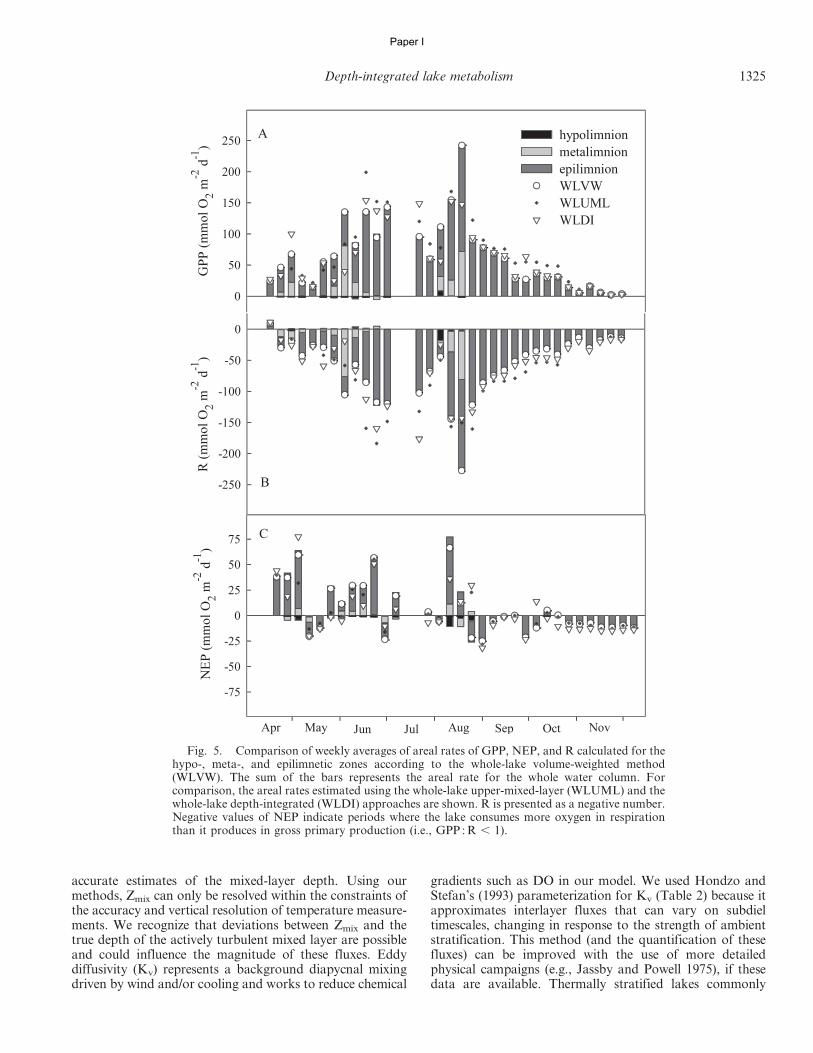
accurate estimates of the mixed-layer depth. Using ourmethods, Zmix can only be resolved within the constraints ofthe accuracy and vertical resolution of temperature measure-ments. We recognize that deviations between Zmix and thetrue depth of the actively turbulent mixed layer are possibleand could influence the magnitude of these fluxes. Eddydiffusivity (Kv) represents a background diapycnal mixingdriven by wind and/or cooling and works to reduce chemical

gradients such as DO in our model. We used Hondzo andStefan’s (1993) parameterization for Kv (Table 2) because itapproximates interlayer fluxes that can vary on subdieltimescales, changing in response to the strength of ambientstratification. This method (and the quantification of thesefluxes) can be improved with the use of more detailedphysical campaigns (e.g., Jassby and Powell 1975), if thesedata are available. Thermally stratified lakes commonly

Fig. 5. Comparison of weekly averages of areal rates of GPP, NEP, and R calculated for thehypo-, meta-, and epilimnetic zones according to the whole-lake volume-weighted method(WLVW). The sum of the bars represents the areal rate for the whole water column. Forcomparison, the areal rates estimated using the whole-lake upper-mixed-layer (WLUML) and thewhole-lake depth-integrated (WLDI) approaches are shown. R is presented as a negative number.Negative values of NEP indicate periods where the lake consumes more oxygen in respirationthan it produces in gross primary production (i.e., GPP : R , 1).

Depth-integrated lake metabolism 1325

Paper I

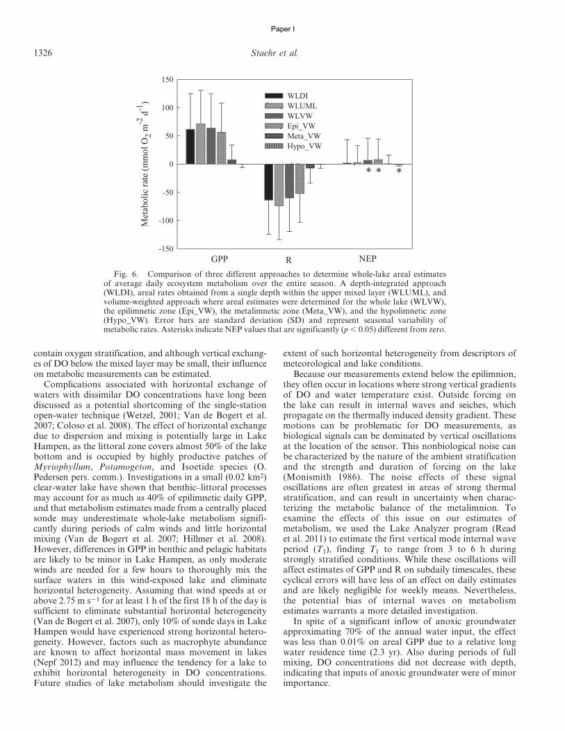
contain oxygen stratification, and although vertical exchang-es of DO below the mixed layer may be small, their influenceon metabolic measurements can be estimated.

Complications associated with horizontal exchange ofwaters with dissimilar DO concentrations have long beendiscussed as a potential shortcoming of the single-stationopen-water technique (Wetzel, 2001; Van de Bogert et al.2007; Coloso et al. 2008). The effect of horizontal exchangedue to dispersion and mixing is potentially large in LakeHampen, as the littoral zone covers almost 50% of the lakebottom and is occupied by highly productive patches ofMyriophyllum, Potamogeton, and Isoetide species (O.Pedersen pers. comm.). Investigations in a small (0.02 km2)clear-water lake have shown that benthic–littoral processesmay account for as much as 40% of epilimnetic daily GPP,and that metabolism estimates made from a centrally placedsonde may underestimate whole-lake metabolism signifi-cantly during periods of calm winds and little horizontalmixing (Van de Bogert et al. 2007; Hillmer et al. 2008).However, differences in GPP in benthic and pelagic habitatsare likely to be minor in Lake Hampen, as only moderatewinds are needed for a few hours to thoroughly mix thesurface waters in this wind-exposed lake and eliminatehorizontal heterogeneity. Assuming that wind speeds at orabove 2.75 m s21 for at least 1 h of the first 18 h of the day issufficient to eliminate substantial horizontal heterogeneity(Van de Bogert et al. 2007), only 10% of sonde days in LakeHampen would have experienced strong horizontal hetero-geneity. However, factors such as macrophyte abundanceare known to affect horizontal mass movement in lakes(Nepf 2012) and may influence the tendency for a lake toexhibit horizontal heterogeneity in DO concentrations.Future studies of lake metabolism should investigate the

extent of such horizontal heterogeneity from descriptors ofmeteorological and lake conditions.

Because our measurements extend below the epilimnion,they often occur in locations where strong vertical gradientsof DO and water temperature exist. Outside forcing onthe lake can result in internal waves and seiches, whichpropagate on the thermally induced density gradient. Thesemotions can be problematic for DO measurements, asbiological signals can be dominated by vertical oscillationsat the location of the sensor. This nonbiological noise canbe characterized by the nature of the ambient stratificationand the strength and duration of forcing on the lake(Monismith 1986). The noise effects of these signaloscillations are often greatest in areas of strong thermalstratification, and can result in uncertainty when charac-terizing the metabolic balance of the metalimnion. Toexamine the effects of this issue on our estimates ofmetabolism, we used the Lake Analyzer program (Readet al. 2011) to estimate the first vertical mode internal waveperiod (T1), finding T1 to range from 3 to 6 h duringstrongly stratified conditions. While these oscillations willaffect estimates of GPP and R on subdaily timescales, thesecyclical errors will have less of an effect on daily estimatesand are likely negligible for weekly means. Nevertheless,the potential bias of internal waves on metabolismestimates warrants a more detailed investigation.

In spite of a significant inflow of anoxic groundwaterapproximating 70% of the annual water input, the effectwas less than 0.01% on areal GPP due to a relative longwater residence time (2.3 yr). Also during periods of fullmixing, DO concentrations did not decrease with depth,indicating that inputs of anoxic groundwater were of minorimportance.

Fig. 6. Comparison of three different approaches to determine whole-lake areal estimatesof average daily ecosystem metabolism over the entire season. A depth-integrated approach(WLDI), areal rates obtained from a single depth within the upper mixed layer (WLUML), andvolume-weighted approach where areal estimates were determined for the whole lake (WLVW),the epilimnetic zone (Epi_VW), the metalimnetic zone (Meta_VW), and the hypolimnetic zone(Hypo_VW). Error bars are standard deviation (SD) and represent seasonal variability ofmetabolic rates. Asterisks indicate NEP values that are significantly (p , 0.05) different from zero.

1326 Staehr et al.

Paper I

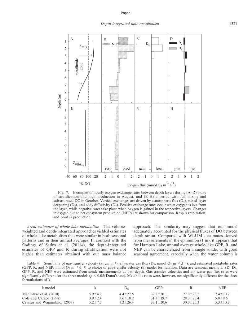
Areal estimates of whole-lake metabolism—The volume-weighted and depth-integrated approaches yielded estimatesof whole-lake metabolism that were similar in both seasonalpatterns and in their annual averages. In contrast with thefindings of Sadro et al. (2011a), the depth-integratedestimates of GPP and R during stratification were nothigher than estimates obtained with our mass balance

approach. This similarity may suggest that our modeladequately accounted for the physical fluxes of DO betweendepth strata. Compared with WLUML estimates derivedfrom measurements in the epilimnion (1 m), it appears thatfor Hampen Lake, annual average whole-lake GPP, R, andNEP can be characterized from a single sonde, with goodseasonal agreement, especially when the water column is

Fig. 7. Examples of hourly oxygen exchange rates between depth layers during (A–D) a dayof stratification and high production in August, and (E–H) a period with full mixing andsubsaturated DO in October. Vertical exchanges are driven by atmospheric flux (Ds), mixed-layerdeepening (Dz), and eddy diffusivity (Dv). Positive exchange rates occur when oxygen is lost fromthe layer, while negative rates take place when oxygen is gained in the respective layers. Changesin oxygen due to net ecosystem production (NEP) are shown for comparison. Resp is respiration,and prod is production.

Table 4. Sensitivity of gas-transfer velocity (k; cm h21), air–water gas flux (Ds; mmol O2 m22 d21), and estimated metabolic rates(GPP, R, and NEP; mmol O2 m23 d21) to choice of gas-transfer velocity (k) model formulation. Data are seasonal means 6 SD. DS,GPP, R, and NEP were estimated from sonde measurements at 1-m depth. Gas-transfer velocities and air–water gas flux rates weresignificantly different for the three models (p , 0.05; Dunn’s test). Metabolic rates were, however, not significantly different for the threeformulations of k.

k-model k DS GPP R NEP

MacIntyre et al. (2010) 5.964.2 4.4627.5 32.2620.1 27.0620.5 7.4610.7Cole and Caraco (1998) 3.962.4 3.6618.2 31.3619.7 28.3620.4 5.069.6Crusius and Wanninkhof (2003) 5.267.7 3.2626.4 33.1620.6 30.0620.3 5.3610.3

Depth-integrated lake metabolism 1327

Paper I

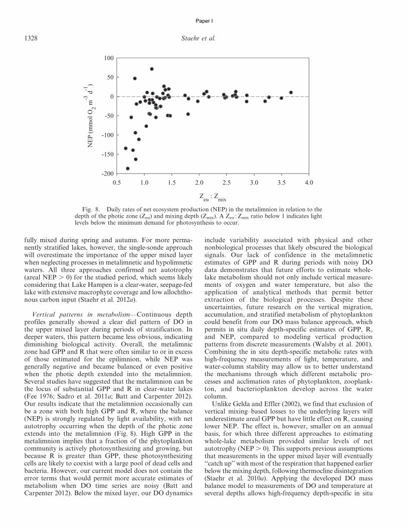
fully mixed during spring and autumn. For more perma-nently stratified lakes, however, the single-sonde approachwill overestimate the importance of the upper mixed layerwhen neglecting processes in metalimnetic and hypolimneticwaters. All three approaches confirmed net autotrophy(areal NEP . 0) for the studied period, which seems likelyconsidering that Lake Hampen is a clear-water, seepage-fedlake with extensive macrophyte coverage and low allochtho-nous carbon input (Staehr et al. 2012a).

Vertical patterns in metabolism—Continuous depthprofiles generally showed a clear diel pattern of DO inthe upper mixed layer during periods of stratification. Indeeper waters, this pattern became less obvious, indicatingdiminishing biological activity. Overall, the metalimniczone had GPP and R that were often similar to or in excessof those estimated for the epilimnion, while NEP wasgenerally negative and became balanced or even positivewhen the photic depth extended into the metalimnion.Several studies have suggested that the metalimnion can bethe locus of substantial GPP and R in clear-water lakes(Fee 1976; Sadro et al. 2011a; Batt and Carpenter 2012).Our results indicate that the metalimnion occasionally canbe a zone with both high GPP and R, where the balance(NEP) is strongly regulated by light availability, with netautotrophy occurring when the depth of the photic zoneextends into the metalimnion (Fig. 8). High GPP in themetalimnion implies that a fraction of the phytoplanktoncommunity is actively photosynthesizing and growing, butbecause R is greater than GPP, these photosynthesizingcells are likely to coexist with a large pool of dead cells andbacteria. However, our current model does not contain theerror terms that would permit more accurate estimates ofmetabolism when DO time series are noisy (Batt andCarpenter 2012). Below the mixed layer, our DO dynamics

include variability associated with physical and othernonbiological processes that likely obscured the biologicalsignals. Our lack of confidence in the metalimneticestimates of GPP and R during periods with noisy DOdata demonstrates that future efforts to estimate whole-lake metabolism should not only include vertical measure-ments of oxygen and water temperature, but also theapplication of analytical methods that permit betterextraction of the biological processes. Despite theseuncertainties, future research on the vertical migration,accumulation, and stratified metabolism of phytoplanktoncould benefit from our DO mass balance approach, whichpermits in situ daily depth-specific estimates of GPP, R,and NEP, compared to modeling vertical productionpatterns from discrete measurements (Walsby et al. 2001).Combining the in situ depth-specific metabolic rates withhigh-frequency measurements of light, temperature, andwater-column stability may allow us to better understandthe mechanisms through which different metabolic pro-cesses and acclimation rates of phytoplankton, zooplank-ton, and bacterioplankton develop across the watercolumn.

Unlike Gelda and Effler (2002), we find that exclusion ofvertical mixing–based losses to the underlying layers willunderestimate areal GPP but have little effect on R, causinglower NEP. The effect is, however, smaller on an annualbasis, for which three different approaches to estimatingwhole-lake metabolism provided similar levels of netautotrophy (NEP . 0). This supports previous assumptionsthat measurements in the upper mixed layer will eventually‘‘catch up’’ with most of the respiration that happened earlierbelow the mixing depth, following thermocline disintegration(Staehr et al. 2010a). Applying the developed DO massbalance model to measurements of DO and temperature atseveral depths allows high-frequency depth-specific in situ

Fig. 8. Daily rates of net ecosystem production (NEP) in the metalimnion in relation to thedepth of the photic zone (Zeu) and mixing depth (Zmix). A Zeu : Zmix ratio below 1 indicates lightlevels below the minimum demand for photosynthesis to occur.

1328 Staehr et al.

Paper I

rates of primary production and respiration to be calculated,which could improve future investigations of physiologicalacclimation in vertically migrating planktonic organisms.

The profiling application is recommended for estima-tion of metabolic rates in stratified lakes, as measurementsof oxygen can be used to account for vertical exchangebetween epilimnetic and hypolimnetic waters. Futurestudies based on high-frequency measurements at multipledepths should be coupled with a thorough signal-processinganalysis in order to remove confounding sources of errorfrom the DO time series. Depth-specific metabolic rates canprovide insight into important metabolic processes occur-ring in the metalimnion, as well as accounting for benthicmetabolism. We demonstrated that metabolism belowmixed-layer depth was not negligible and its assessmentenhanced our understanding of the magnitude and spatio-temporal dynamics of carbon mineralization and fixation,and thus the generation of a resource that may support theecosystem’s food web. Application of profiled oxygenmeasurements accordingly reveals patterns in metabolismthat may have important implications for our interpretationof carbon cycling in stratifying lakes.

AcknowledgmentsWe are grateful for valuable comments by Steven Sadro and

three anonymous reviewers, as well as the technical assistance ofLars Baastrup-Spohr, Birgit Kjøller, and Flemming Brundam.This study was financed by The Danish Council for IndependentResearch | Natural Sciences grants 272-05-0277 and 10-085238,and supported by the Danish Centre for Lake Restoration(CLEAR) and the Danish Strategic Research Council, ‘‘Monitor-ing remote environments with Autonomous sensor Network-based data Acquisition’’ (MANA). J.S.R. was supported by U.S.National Science Foundation (NSF) grant DEB-0822700.

References

BATT, R. D., AND S. R. CARPENTER. 2012. Free-water lake metabolism:Addressing noisy time series with a Kalman filter. Limnol.Oceanogr.: Methods 10: 20–30, doi:10.4319/lom.2012.10.20

BELL, V. A., D. G. GEORGE, R. J. MOORE, AND J. PARKER. 2006.Using a 1-D mixing model to simulate the vertical flux of heatand oxygen in a lake subject to mixing. Ecol. Model. 190:41–54, doi:10.1016/j.ecolmodel.2005.02.025

BELLA, D. A. 1970. Dissolved oxygen variations in stratified lakes.J. Sanit. Eng. Div. 96: 1129–1146.

BOEGMAN, L., G. N. IVEY, AND J. IMBERGER. 2005. The energeticsof large-scale internal wave degeneration in lakes. J. FluidMech. 531: 159–180, doi:10.1017/S0022112005003915

CAFFREY, J. M. 2003. Production, respiration and net ecosystemmetabolism in U.S. estuaries. Environ. Monit. Assess. 81:207–219, doi:10.1023/A:1021385226315

CARACO, N. F., AND J. J. COLE. 2002. Contrasting impacts of anative and alien macrophyte on dissolved oxygen in a largeriver. Ecol. Appl. 12: 1496–1509, doi:10.1890/1051-0761(2002)012[1496:CIOANA]2.0.CO;2

COLE, J. J., AND N. F. CARACO. 1998. Atmospheric exchange ofcarbon dioxide in a low-wind oligotrophic lake measured bythe addition of SF6. Limnol. Oceanogr. 43: 647–656, doi:10.4319/lo.1998.43.4.0647

———, M. L. PACE, S. R. CARPENTER, AND J. F. KITCHELL. 2000.Persistence of net heterotrophy in lakes during nutrient

addition and food web manipulations. Limnol. Oceanogr.45: 1718–1730, doi:10.4319/lo.2000.45.8.1718

COLOSO, J. J., J. J. COLE, P. C. HANSON, AND M. L. PACE. 2008.Depth-integrated, continuous estimates of metabolism in aclear-water lake. Can. J. Fish. Aquat. Sci. 65: 712–722, doi:10.1139/f08-006

CRUSIUS, J., AND R. WANNINKHOF. 2003. Gas transfer velocitiesmeasured at low wind speed over a lake. Limnol. Oceanogr.48: 1010–1017, doi:10.4319/lo.2003.48.3.1010

DOWNING, J. A., AND OTHERS. 2006. The global abundance and sizedistribution of lakes, ponds, and impoundments. Limnol.Oceanogr. 51: 2388–2397, doi:10.4319/lo.2006.51.5.2388

EATON, A. D., L. S. CLESCERI, A. E. GREENBERG, AND M. A. H.FRANSON [EDS.]. 1995. Standard methods for examination of waterand waste water, 19th ed. American Public Health Association.

FEE, E. J. 1976. Vertical and seasonal distribution of chlorophyllin lakes of experimental-lakes-area, Northwestern Ontario—implications for primary production estimates. Limnol.Oceanogr. 21: 767–783, doi:10.4319/lo.1976.21.6.0767

GELDA, R. K., AND S. W. EFFLER. 2002. Metabolic rate estimatesfor a eutrophic lake from diel dissolved oxygen signals.Hydrobiologia 485: 51–66, doi:10.1023/A:1021327610570

HANSON, P. C., D. L. BADE, AND S. R. CARPENTER. 2003. Lakemetabolism: Relationships with dissolved organic carbon andphosphorus. Limnol. Oceanogr. 48: 1112–1119, doi:10.4319/lo.2003.48.3.1112

HILLMER, I., P. VAN REENEN, J. IMBERGER, AND T. ZOHARY. 2008.Phytoplankton patchiness and their role in the modelledproductivity of a large, seasonally stratified lake. Ecol. Model.218: 49–59, doi:10.1016/j.ecolmodel.2008.06.017

HONDZO, M., AND H. G. STEFAN. 1993. Lake water temperaturesimulation model. J. Hydraul. Eng. ASCE 119: 1251–1273,doi:10.1061/(ASCE)0733-9429(1993)119:11(1251)

HORNBERGER, G. M., AND G. KELLY. 1974. A new method forestimating productivity in standing waters using free oxygenmeasurements. Water Resour. Bull. 10: 265–271, doi:10.1111/j.1752-1688.1974.tb00565.x

IMBERGER, J. 1985. The diurnal mixed layer. Limnol. Oceanogr.30: 737–770, doi:10.4319/lo.1985.30.4.0737

JAHNE, B., O. MUNNICH, R. BOSINGER, A. DUTZI, W. HUBER, AND

P. LIBNER. 1987. On the parameters influencing air-watergas exchange. J. Geophys. Res. 92: 1937–1949, doi:10.1029/JC092iC02p01937

JASSBY, A., AND T. POWELL. 1975. Vertical patterns of eddy diffusionduring stratification in Castle Lake, California. Limnol.Oceanogr. 20: 530–543, doi:10.4319/lo.1975.20.4.0530

JESPERSEN, A. M., AND K. CHRISTOFFERSEN. 1987. Measurementsof chlorophyll a from phytoplankton using ethanol asextraction solvent. Archiv Hydrobiol. 109: 445–454.

JONAS, T., A. STIPS, W. EUGSTER, AND A. WUEST. 2003. Observationsof a quasi shear-free lacustrine convective boundary layer:Stratification and its implications on turbulence. J. Geophys.Res. Oceans 108, (C10), doi:10.1029/2002JC001440

KIDMOSE, J., P. ENGESGAARD, B. NILSSON, T. LAIER, AND M. C.LOOMS. 2011. Spatial distribution of seepage at a flow-throughlake: Lake Hampen, Western Denmark. Vadose Zone J. 10:110–124, doi:10.2136/vzj2010.0017

KRAGH, T., AND M. SONDERGAARD. 2004. Production andbioavailability of autochthonous dissolved organic carbon:Effects of mesozooplankton. Aquat. Microb. Ecol. 36: 61–72,doi:10.3354/ame036061

LAUSTER, G. H., P. C. HANSON, AND T. K. KRATZ. 2006. Grossprimary production and respiration differences among littoraland pelagic habitats in northern Wisconsin lakes. Can. J.Fish. Aquat. Sci. 63: 1130–1141, doi:10.1139/f06-018

Depth-integrated lake metabolism 1329

Paper I

MACINTYRE, S., K. M. FLYNN, R. JELLISON, AND J. R. ROMERO. 1999.Boundary mixing and nutrient fluxes in Mono Lake, California.Limnol. Oceanogr. 44: 512–529, doi:10.4319/lo.1999.44.3.0512

———, A. JONSSON, M. JANSSON, J. ABERG, D. E. TURNEY, AND

S. D. MILLER. 2010. Buoyancy flux, turbulence, and the gastransfer coefficient in a stratified lake. Geophys. Res. Lett. 37:L24604, doi:10.1029/2010GL044164

MELACK, J. M. 1982. Photosynthetic activity and respiration in anequatorial African soda lake. Freshw. Biol. 12: 381–399, doi:10.1111/j.1365-2427.1982.tb00631.x

MONISMITH, S. 1986. An experimental study of the upwellingresponse of stratified reservoirs to surface shear-stresses.J. Fluid Mech. 171: 407–439, doi:10.1017/S0022112086001507

NEPF, H. M. 2012. Flow and transport in regions with aquaticvegetation. Ann. Rev. Fluid Mech. 44: 123–42, doi:10.1146/annurev-fluid-120710-101048

ODUM, H. T. 1956. Primary production in flowing waters. Limnol.Oceanogr. 1: 102–117, doi:10.4319/lo.1956.1.2.0102

PACE, M. L., AND Y. T. PRAIRIE. 2005. Respiration in lakes,p. 103–121. In P. J. le. B. Williams and P. A. del Giorgio[eds.], Respiration in aquatic ecosystems. Oxford Univ. Press.

READ, J. S., AND OTHERS. 2011. Derivation of lake mixing andstratification indices from high-resolution lake buoy data. Environ.Model. Softw. 26: 1325–1336, doi:10.1016/j.envsoft.2011.05.006

RIMMER, A., M. BOGER, Y. AOTA, AND M. KUMAGAI. 2006. A lakeas a natural integrator of linear processes: Application toLake Kinneret (Israel) and Lake Biwa (Japan). J. Hydrol. 319:163–175, doi:10.1016/j.jhydrol.2005.07.018

SADRO, S., J. M. MELACK, AND S. MACINTYRE. 2011a. Depth-integrated estimates of ecosystem metabolism in a high-elevationlake (Emerald Lake, Sierra Nevada, California). Limnol.Oceanogr. 56: 1764–1780, doi:10.4319/lo.2011.56.5.1764

———, C. E. NELSON, AND J. M. MELACK. 2011b. Linking dielpatterns in community respiration to bacterioplankton in anoligotrophic high-elevation lake. Limnol. Oceanogr. 56:540–550, doi:10.4319/lo.2011.56.2.0540

SMITH, S. V. 1985. Physical, chemical and biological characteristics ofCO2 gas flux across the air-water interface. Plant, Cell Environ.8: 387–398, doi:10.1111/j.1365-3040.1985.tb01674.x

STAEHR, P. A., L. BAASTRUP-SPOHR, K. SAND-JENSEN, AND

C. STEDMON. 2012a. Lake metabolism scales with lake

morphometry and catchment conditions. Aquat. Sci. 74:155–169, doi:10.1007/s00027-011-0207-6

———, AND K. SAND-JENSEN. 2007. Temporal dynamics andregulation of lake metabolism. Limnol. Oceanogr. 52:108–120, doi:10.4319/lo.2007.52.1.0108

———, ———, A. L. RAUN, B. NIELSSON, AND J. KIDMOSE. 2010a.Drivers of metabolism and net heterotrophy in contrasting lakes.Limnol. Oceanogr. 55: 817–830, doi:10.4319/lo.2009.55.2.0817

———, J. TESTA, M. KEMP, J. J. COLE, K. SAND-JENSEN, AND S. V.SMITH. 2012b. The metabolism of aquatic ecosystems: History,applications, and future challenges. Aquat. Sci. 74: 15–29,doi:10.1007/s00027-011-0199-2

———, AND OTHERS. 2010b. Lake metabolism and the diel oxygentechnique: State of the science. Limnol. Oceanogr.: Methods8: 628–644, doi:10.4319/lom.2010.8.0628

TOBIAS, C. R., J. K. BOLKE, AND W. HARVEY. 2007. The oxygen-18isotope approach for measuring aquatic metabolism in high-productive waters. Limnol. Oceanogr. 52: 1439–1453,doi:10.4319/lo.2007.52.4.1439

VAN DE BOGERT, M. C., S. R. CARPENTER, J. J. COLE, AND M. L.PACE. 2007. Assessing pelagic benthic metabolism using freewater measurements. Limnol. Oceanogr.: Methods 5:145–155, doi:10.4319/lom.2007.5.145

WALSBY, A. E., Z. DUBINSKY, J. C. KROMKAMP, C. LEHMANN, AND

F. SCHANZ. 2001. The effects of diel changes in photosyntheticcoefficients and depth of Planktothrix rubescens on the dailyintegral of photosynthesis in Lake Zurich. Aquat. Sci. 63:326–349, doi:10.1007/PL00001358

WANNINKHOF, R. 1992. Relationship between wind speed and gasexchange over the ocean. J. Geophys. Res. 97: 7373–7382,doi:10.1029/92JC00188

WETZEL, R. 2001. Lake and river ecosystems. Academic Press.

Associate editor: George W. Kling

Received: 17 June 2011Accepted: 12 March 2012

Amended: 10 April 2012

1330 Staehr et al.

Paper I

38

Paper II

Why bother about depth? Relevance of metabolism below the upper mixed layer in 1

lakes 2 Biel Obrador

1*, Peter A. Staehr

2 and Jesper P.C. Christensen

2,3 3

4 1University of Barcelona, Department of Ecology, Barcelona, Spain 5

2University of Aarhus, Institute of Bioscience, Roskilde, Denmark 6

3Freshwater Biological Section, University of Copenhagen, Copenhagen, Denmark 7

8 *Corresponding author: obrador@ub.edu 9 10 Running head: 11 Depth dependent metabolism in lakes 12 13

Paper II

Obrador, Staehr & Christensen Depth dependent metabolism in lakes

Page 2/29

Acknowledgements 14 The NETLAKE - NETworking LAKe observatories in Europe made this analysis possible. 15 Network-level activities of NETLAKE are funded in by the European Research Council 16 COST action ES1201. BO was supported by the Spanish Ministry of Education (José 17 Castillejo grant no JC2011-0111) and by the Spanish Ministry of Science (project 18 CARBONET, Carbon transport and use through river networks: the relevance of global 19 change, CGL2011-30474-C02-0). PAS was supported by the Danish Council for Independent 20 Research ǀ Natural Sciences grant no 10-085238, and by the Danish Centre for Lake 21 Restoration (CLEAR). JPC was supported by the Danish strategic research council; 22 Monitoring remote environments with Autonomous sensor Network-based data Acquisition" 23 (MANA). We are grateful to Chris Salomon for constructive comments. 24

25

Paper II

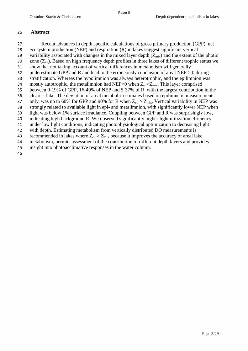
Obrador, Staehr & Christensen Depth dependent metabolism in lakes

Page 3/29

Abstract 26

Recent advances in depth specific calculations of gross primary production (GPP), net 27 ecosystem production (NEP) and respiration (R) in lakes suggest significant vertical 28 variability associated with changes in the mixed layer depth (Zmix) and the extent of the photic 29 zone (Zeu). Based on high frequency depth profiles in three lakes of different trophic status we 30 show that not taking account of vertical differences in metabolism will generally 31 underestimate GPP and R and lead to the erroneously conclusion of areal NEP > 0 during 32 stratification. Whereas the hypolimnion was always heterotrophic, and the epilimnion was 33 mostly autotrophic, the metalimnion had NEP>0 when Zeu>Zmix. This layer comprised 34 between 0-19% of GPP, 16-49% of NEP and 5-37% of R, with the largest contribution in the 35 clearest lake. The deviation of areal metabolic estimates based on epilimnetic measurements 36 only, was up to 60% for GPP and 90% for R when Zeu > Zmix. Vertical variability in NEP was 37 strongly related to available light in epi- and metalimnion, with significantly lower NEP when 38 light was below 1% surface irradiance. Coupling between GPP and R was surprisingly low, 39

indicating high background R. We observed significantly higher light utilization efficiency 40 under low light conditions, indicating photophysiological optimization to decreasing light 41 with depth. Estimating metabolism from vertically distributed DO measurements is 42 recommended in lakes where Zeu > Zmix because it improves the accuracy of areal lake 43 metabolism, permits assessment of the contribution of different depth layers and provides 44 insight into photoacclimative responses in the water column. 45

46

Paper II

Obrador, Staehr & Christensen Depth dependent metabolism in lakes

Page 4/29

Introduction 47 Measurements of the production and consumption of organic material has been a focus 48

of aquatic science for more than 80 years during which an important aim has been to quantify 49 the magnitude and understand the drivers of variability of metabolic rates and carbon 50 processing (Staehr et al. 2012a). Measurement of diel, “free-water” changes in dissolved 51 oxygen (DO) concentrations has become a widely accepted method to examine whole-52 ecosystem primary production and respiration, particularly popular in lakes (Cole et al. 2000; 53 Gelda and Effler 2002; Staehr et al. 2010a). The popularity of the diel, “free-water” technique 54 among researchers and managers relates to awareness that it is important to capture the often 55 highly variable temporal dynamics which can be obtained by a continuous monitoring 56 approach (Staehr and Sand-Jensen 2007) which strengthen predictions of how changes in 57 environmental conditions (e.g., climate, deforestation, and eutrophication) affect lakes 58 (Hanson et al. 2006; Williamson et al. 2008; Staehr et al. 2012b). 59

The basic assumption behind and generally accepted advantage of the open water diel 60

DO technique is that the diel change in DO in the water column is an integrated response to 61 the metabolism of the entire ecosystem (all autotrophs and heterotrophs). However, as the use 62 of free-water techniques has expanded, new insights and new questions have emerged on the 63 validity of the metabolic estimates (Staehr and Sand-Jensen 2007; Hanson et al. 2008; Sadro 64 et al. 2011a), and the extent to which free-water measurements actually represent whole-lake 65 metabolism (Lauster et al. 2006; Van de Bogert et al. 2007; Staehr et al. 2010a). A major 66 concern relates to vertical heterogeneity of the DO signal in lakes deep enough to experience 67 vertical temperature stratification. For clear water lakes, the photic zone may extend below 68 the thermocline resulting in primary production that is not measured by a sonde in the upper 69 mixed layer, thereby underestimating whole-lake areal gross primary production (Coloso et 70 al. 2008). Light availability is, however, not sufficient to support pelagic primary production 71 below the metalimnion in most stratified lakes. But because respiration occurs at all depths, 72 and appears to be unrelated to depth, calculation of areal rates using epilimnetic data only, 73 would significantly underestimate R (Coloso et al. 2008; Staehr et al. 2012c). The extent to 74

which this produces an uncertainty in whole-lake metabolism estimates depends on the 75 duration and strength of the stratification as well as the volume of water in the hypolimnion 76 (Sadro et al. 2011a; Staehr et al. 2012c). This is an issue in most tropical lakes more than a 77

few meters deep, and a reoccurring problem in temperate lakes during summer, especially in 78 sheltered, deep and darkly stained lakes (Staehr et al. 2010b). Furthermore, epilimnetic sonde 79 measurements are unable to quantify benthic metabolism during periods of stratification. It 80 would therefore be were useful with a cross lake comparison the importance of metabolic 81 rates below the upper mixed layer. 82

Only a few studies have investigated the importance of vertical heterogeneity in DO for 83 evaluating lake metabolism with the diel DO technique (Gelda and Effler 2002; Coloso et al. 84

2008; Sadro et al. 2011a) and only in a recent study was daily variability in metabolism 85 evaluated at discrete depths throughout the water column (Staehr et al. 2012c). Their findings 86

indicate that the metalimnion is an intensive zone of primary production when sufficient light 87 is available and nutrient levels are depleted in the upper mixed layer. This agrees well with 88 the conceptual model proposed by Kalff (2002) that vertical patterns in water column 89 productivity is controlled by variations in mixed layer depth (Zmix) and water clarity through 90 regulation of light and nutrient availability. 91

In this paper we use a unique dataset of high frequency oxygen and temperature profiles 92 in three lakes of different trophic status to test existing models of variability in lake 93

Paper II

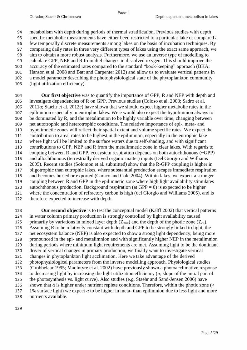
Obrador, Staehr & Christensen Depth dependent metabolism in lakes

Page 5/29

metabolism with depth during periods of thermal stratification. Previous studies with depth 94

specific metabolic measurements have either been restricted to a particular lake or compared a 95 few temporally discrete measurements among lakes on the basis of incubation techniques. By 96 comparing daily rates in three very different types of lakes using the exact same approach, we 97 aim to obtain a more robust analysis. Furthermore, we use an inverse type of modelling to 98 calculate GPP, NEP and R from diel changes in dissolved oxygen. This should improve the 99 accuracy of the estimated rates compared to the standard “book-keeping” approach (BKA; 100 Hanson et al. 2008 and Batt and Carpenter 2012) and allow us to evaluate vertical patterns in 101 a model parameter describing the photophysiological state of the phytoplankton community 102 (light utilization efficiency). 103

Our first objective was to quantify the importance of GPP, R and NEP with depth and 104 investigate dependencies of R on GPP. Previous studies (Coloso et al. 2008; Sadro et al. 105 2011a; Staehr et al. 2012c) have shown that we should expect higher metabolic rates in the 106 epilimnion especially in eutrophic lakes. We e would also expect the hypolimnion always to 107

be dominated by R, and the metalimnion to be highly variable over time, changing between 108 net autotrophic and heterotrophic conditions. The relative importance of epi-, meta- and 109 hypolimnetic zones will reflect their spatial extent and volume specific rates. We expect the 110 contribution to areal rates to be highest in the epilimnion, especially in the eutrophic lake 111 where light will be limited to the surface waters due to self-shading, and with significant 112 contributions to GPP, NEP and R from the metalimnetic zone in clear lakes. With regards to 113 coupling between R and GPP, ecosystem respiration depends on both autochthonous (~GPP) 114 and allochthonous (terrestrially derived organic matter) inputs (Del Giorgio and Williams 115 2005). Recent studies (Solomon et al. submitted) show that the R-GPP coupling is higher in 116 oligotrophic than eutrophic lakes, where substantial production escapes immediate respiration 117 and becomes buried or exported (Caraco and Cole 2004). Within lakes, we expect a stronger 118 coupling between R and GPP in the epilimnetic zone where high light availability stimulates 119 autochthonous production. Background respiration (at GPP = 0) is expected to be higher 120 where the concentration of refractory carbon is high (del Giorgio and Williams 2005), and is 121

therefore expected to increase with depth. 122

Our second objective is to test the conceptual model (Kalff 2002) that vertical patterns 123 in water column primary production is strongly controlled by light availability caused 124

primarily by variations in mixed layer depth (Zmix) and the depth of the photic zone (Zeu). 125 Assuming R to be relatively constant with depth and GPP to be strongly linked to light, the 126

net ecosystem balance (NEP) is also expected to show a strong light dependency, being more 127 pronounced in the epi- and metalimnion and with significantly higher NEP in the metalimnion 128 during periods where minimum light requirements are met. Assuming light to be the dominant 129

driver of vertical changes in primary production, we finally want to investigate vertical 130 changes in phytoplankton light acclimation. Here we take advantage of the derived 131

photophysiological parameters from the inverse modelling approach. Physiological studies 132 (Grobbelaar 1995; MacIntyre et al. 2002) have previously shown a photoacclimative response 133

to decreasing light by increasing the light utilization efficiency (α; slope of the initial part of 134 the photosynthesis vs. light curve). Also studies (e.g. Staehr and Sand-Jensen 2006) have 135 shown that α is higher under nutrient replete conditions. Therefore, within the photic zone (> 136 1% surface light) we expect α to be higher in meta- than epilimnion due to less light and more 137 nutrients available. 138

139

Paper II

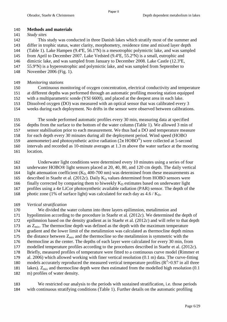
Obrador, Staehr & Christensen Depth dependent metabolism in lakes

Page 6/29

Methods and materials 140 Study sites 141

This study was conducted in three Danish lakes which stratify most of the summer and 142 differ in trophic status, water clarity, morphometry, residence time and mixed layer depth 143 (Table 1). Lake Hampen (9.4ºE, 56.1ºN) is a mesotrophic polymictic lake, and was sampled 144 from April to December 2007. Lake Vedsted (9.4ºE, 55.2ºN) is a small, eutrophic and 145 dimictic lake, and was sampled from January to December 2008. Lake Castle (12.3ºE, 146 55.9ºN) is a hypereutrophic and polymictic lake, and was sampled from September to 147 November 2006 (Fig. 1). 148

Monitoring stations 149 Continuous monitoring of oxygen concentration, electrical conductivity and temperature 150

at different depths was performed through an automatic profiling mooring station equipped 151 with a multiparametric sonde (YSI 6600), and placed at the deepest area in each lake. 152 Dissolved oxygen (DO) was measured with an optical sensor that was calibrated every 3 153

weeks during each deployment. No drifts in the sensor were observed between calibrations. 154

The sonde performed automatic profiles every 30 min, measuring data at specified 155 depths from the surface to the bottom of the water column (Table 1). We allowed 3 min of 156 sensor stabilisation prior to each measurement. We thus had a DO and temperature measure 157 for each depth every 30 minutes during all the deployment period. Wind speed (HOBO 158 anemometer) and photosynthetic active radiation (2π HOBO

®) were collected at 5-second 159

intervals and recorded as 10-minute averages at 1.3 m above the water surface at the mooring 160 location. 161

Underwater light conditions were determined every 10 minutes using a series of four 162 underwater HOBO® light sensors placed at 20, 40, 80, and 120 cm depth. The daily vertical 163 light attenuation coefficient (KD, 400-700 nm) was determined from these measurements as 164 described in Staehr et al. (2012c). Daily KD values determined from HOBO sensors were 165

finally corrected by comparing them to biweekly KD estimates based on underwater light 166 profiles using a 4π LiCor photosynthetic available radiation (PAR) sensor. The depth of the 167 photic zone (1% of surface light) was calculated for each day as 4.6 / KD. 168

Vertical stratification 169

We divided the water column into three layers epilimnion, metalimnion and 170 hypolimnion according to the procedure in Staehr et al. (2012c). We determined the depth of 171

epilimnion based on the density gradient as in Staehr et al. (2012c) and will refer to that depth 172 as Zmix. The thermocline depth was defined as the depth with the maximum temperature 173 gradient and the lower limit of the metalimnion was calculated as thermocline depth minus 174

the distance between Zmix and the thermocline so the metalimnion is symmetric with the 175 thermocline as the center. The depths of each layer were calculated for every 30 min, from 176

modelled temperature profiles according to the procedures described in Staehr et al. (2012c). 177

Briefly, measured profiles of temperature were fitted to a continuous curve model (Rimmer et 178

al. 2006) which allowed working with finer vertical resolution (0.1 m) data. The curve-fitting 179 models accurately reproduced the measured vertical temperature profiles (R

2>0.97 in all three 180

lakes). Zmix and thermocline depth were then estimated from the modelled high resolution (0.1 181 m) profiles of water density. 182

We restricted our analysis to the periods with sustained stratification, i.e. those periods 183 with continuous stratifying conditions (Table 1). Further details on the automatic profiling 184

Paper II

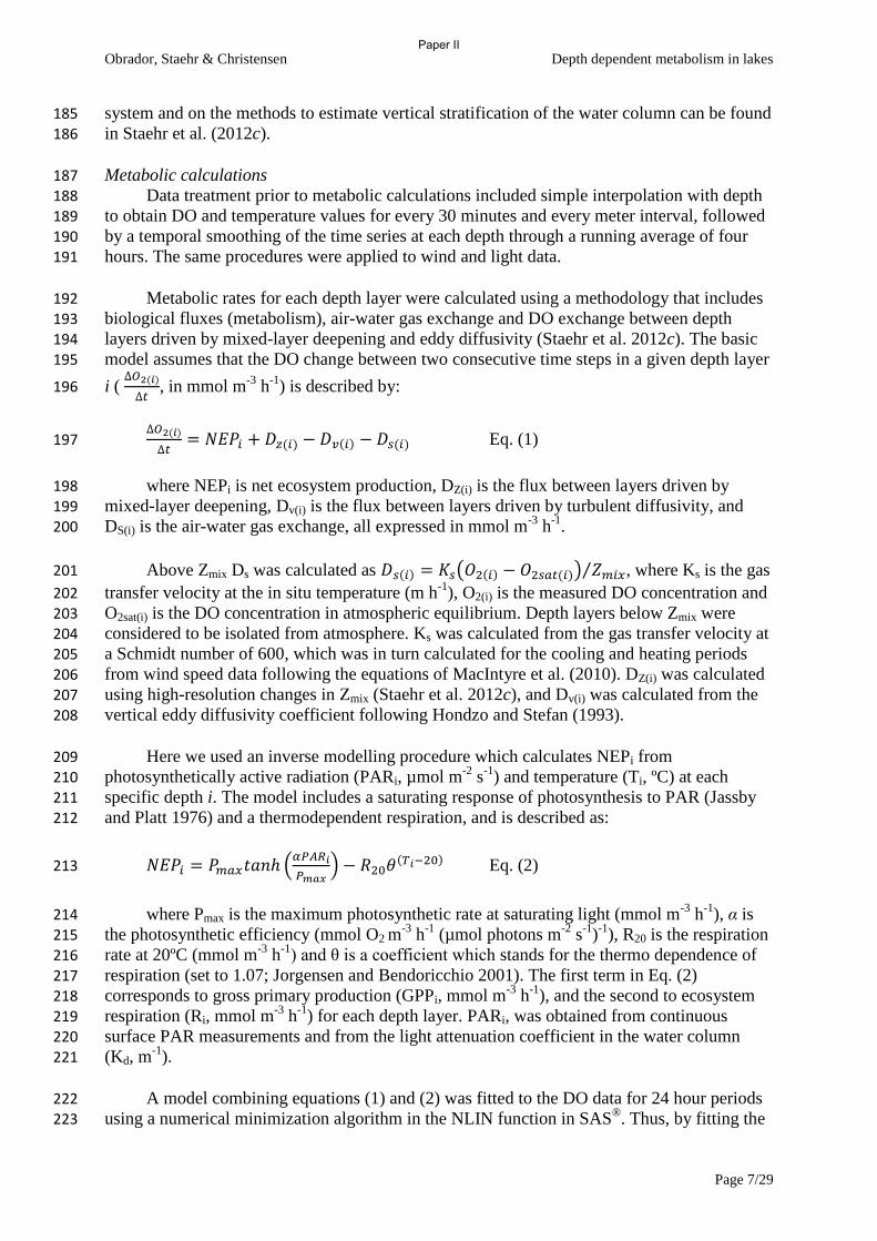
Obrador, Staehr & Christensen Depth dependent metabolism in lakes

Page 7/29

system and on the methods to estimate vertical stratification of the water column can be found 185

in Staehr et al. (2012c). 186

Metabolic calculations 187 Data treatment prior to metabolic calculations included simple interpolation with depth 188

to obtain DO and temperature values for every 30 minutes and every meter interval, followed 189 by a temporal smoothing of the time series at each depth through a running average of four 190 hours. The same procedures were applied to wind and light data. 191

Metabolic rates for each depth layer were calculated using a methodology that includes 192 biological fluxes (metabolism), air-water gas exchange and DO exchange between depth 193 layers driven by mixed-layer deepening and eddy diffusivity (Staehr et al. 2012c). The basic 194 model assumes that the DO change between two consecutive time steps in a given depth layer 195

i (

, in mmol m

-3 h

-1) is described by: 196

Eq. (1) 197

where NEPi is net ecosystem production, DZ(i) is the flux between layers driven by 198 mixed-layer deepening, Dv(i) is the flux between layers driven by turbulent diffusivity, and 199 DS(i) is the air-water gas exchange, all expressed in mmol m

-3 h

-1. 200

Above Zmix Ds was calculated as ( ) ⁄ , where Ks is the gas 201

transfer velocity at the in situ temperature (m h-1

), O2(i) is the measured DO concentration and 202 O2sat(i) is the DO concentration in atmospheric equilibrium. Depth layers below Zmix were 203 considered to be isolated from atmosphere. Ks was calculated from the gas transfer velocity at 204 a Schmidt number of 600, which was in turn calculated for the cooling and heating periods 205 from wind speed data following the equations of MacIntyre et al. (2010). DZ(i) was calculated 206

using high-resolution changes in Zmix (Staehr et al. 2012c), and Dv(i) was calculated from the 207 vertical eddy diffusivity coefficient following Hondzo and Stefan (1993). 208

Here we used an inverse modelling procedure which calculates NEPi from 209 photosynthetically active radiation (PARi, µmol m

-2 s

-1) and temperature (Ti, ºC) at each 210

specific depth i. The model includes a saturating response of photosynthesis to PAR (Jassby 211 and Platt 1976) and a thermodependent respiration, and is described as: 212

(

)

Eq. (2) 213

where Pmax is the maximum photosynthetic rate at saturating light (mmol m-3

h-1

), α is 214 the photosynthetic efficiency (mmol O2 m

-3 h

-1 (µmol photons m

-2 s

-1)-1

), R20 is the respiration 215

rate at 20ºC (mmol m-3

h-1

) and θ is a coefficient which stands for the thermo dependence of 216

respiration (set to 1.07; Jorgensen and Bendoricchio 2001). The first term in Eq. (2) 217

corresponds to gross primary production (GPPi, mmol m-3

h-1

), and the second to ecosystem 218 respiration (Ri, mmol m

-3 h

-1) for each depth layer. PARi, was obtained from continuous 219

surface PAR measurements and from the light attenuation coefficient in the water column 220 (Kd, m

-1). 221

A model combining equations (1) and (2) was fitted to the DO data for 24 hour periods 222

using a numerical minimization algorithm in the NLIN function in SAS®. Thus, by fitting the 223

Paper II

Obrador, Staehr & Christensen Depth dependent metabolism in lakes

Page 8/29

model to the observed DO time series at each depth, we obtained, for every 24-h and every 224

depth layer, estimates of the parameters Pmax, α and R20. We assessed model performance (i.e. 225 how well the model fitted the observed DO data) through the coefficient of determination 226 (R

2). 227

By applying the parameters (Pmax, α and R20) derived in Eq. (2) we calculated hourly 228 metabolic rates for each depth(i) (NEPi, GPPi and Ri, in mmol m

-3 h

-1). Finally, the daily 229

metabolic rates (in mmol m-3

d-1

) were calculated as the average hourly rates multiplied by 24 230 h. Whole-lake areal GPP, R and NEP (mmol m

-2 d

-1) were computed by multiplying the 231

volumetric daily rates of each depth layer (mmol m-3

d-1

) by the water volume within each 232 layer (m

3), and by summing these quantities and dividing by the surface lake area (m

2). 233

Water analysis 234 Biweekly water samples were collected from the epilimnion and measurements of 235

chlorophyll a (Chl a), total phosphorous (TP) and coloured dissolved organic matter 236

(CDOM). Chl a samples were filtered through Advantech 0.7-μm filters, extracted in 96% 237

ethanol for 24 h, and measured according to methods in Jespersen and Christoffersen (1987) 238 using a Shimadzu ultraviolet (UV)-160AH spectrophotometer. Total phosphorus (TP) was 239 determined by persulfate digestion according to Eaton et al. (1995) and further assayed 240 according to Kragh and Sondergaard (2004). Absorbance of CDOM was measured in a GF/F 241 filtrate (0.7 µm) at 360 nm through a 5 cm cuvette. In comprehensive measurements from 242 Danish lakes and streams, DOC concentrations (mg C L

-1) increased linearly with CDOM 243

absorbance at 360 nm (m-1

): DOC = 0.454 CDOM360 +1.9 (r2 =0.80, n = 399, C. Stedmon 244

unpubl.) permitting estimation of DOC from CDOM. 245

Results 246 Vertical patterns in metabolism 247

Within the studied periods, the mixing depth and extent of the metalimnetic zone was 248 smaller and much more variable in the polymictic Hampen Lake compared to the dimictic 249

Vedsted Lake (Fig. 1; Table 1). In comparison, Castle Lake had a stable but narrow 250 metalimnetic zone. Whereas the photic zone always penetrated far into the metalimnion in 251 Hampen Lake, the metalimnion received much less light in Vedsted Lake and 1% light levels 252 were never in the metalimnion in Castle Lake (Fig. 1; Table 1). These results suggest 253 significant differences in the importance of the metalimnetic zones of the three lakes. 254

Although the physical extent of the metalimnion in Hampen Lake was smaller than in 255 Vedsted Lake, the much deeper light penetration, occasionally reaching the hypolimnion, 256 suggests a more intense primary production within the metalimnion in Hampen compared to 257 Vedsted Lake. In comparison, light conditions in the turbid Castle Lake were most likely only 258 able to sustain primary production in the upper mixed layer. 259

Similar vertical patterns in metabolism were observed in the three lakes, with higher 260 GPP and net autotrophy (NEP > 0) in the photic zone and heterotrophy in the layers below the 261

photic depth (Fig. 2 and 3). Accordingly the autotrophic zone extended deeper in Hampen 262 Lake than in Vedsted and was limited to the upper meter in Castle Lake (Fig. 2 and 3). Also, 263

Hampen had larger variability in photic depth (5 to 9 m) resulting in high variability in GPP 264 and NEP within the metalimnion. Whereas heterotrophy progressively increased with depth in 265 Hampen, in Castle and Vedsted Lake maximum heterotrophy occurred in the metalimnion, 266 not in the hypolimnion. The metalimnion was always heterotrophic in Castle Lake (NEP 267 range from -95.1 to -0.7 mmol m

-3 d

-1; mean -26.7; Fig. 3), mostly heterotrophic in Vedsted 268

Lake (NEP range from -81.1 to 63.7 mmol m-3

d-1

; mean -24.1), and varied from 269

Paper II

Obrador, Staehr & Christensen Depth dependent metabolism in lakes

Page 9/29

heterotrophic to slightly autotrophic in Hampen Lake (range from -96.5 to 81.3 mmol m-3

d-1

; 270

mean -7.6). 271

GPP decreased with depth in all three lakes, and the highest GPP was always observed 272 in the epilimnion except in Hampen, where high GPP rates were observed in the metalimnion 273 as well (Fig. 3). All lakes had elevated respiration rates in the metalimnion which often 274 showed the highest rates of the whole water column. Apart from the high R observed in the 275 surface waters of Castle and Vedsted, the maximum respiration rates occurred in the mid 276 metalimnion in Hampen and Vedsted Lake, and in the upper metalimnion and lower 277 epilimnion in Castle Lake (Fig. 3). 278

Differences in the physical structure and light penetration were clearly observed as 279 differences in the contribution of the three depth strata to areal metabolism (Fig. 4; Table 2). 280 Despite the epilimnion was the main contributor to GPP and R of the water column, a 281 considerable contribution of non-epilimnetic waters was observed, especially in Hampen and 282

Vedsted Lake (Table 2). In these lakes, epilimnetic respiration accounted for less than 70% of 283 total respiration. Most of the remaining respiration (about 80%) occurred in the metalimnion 284 (Table 2). Also, the metalimnion accounted for up to 18% of the whole-column GPP on 285 average. In agreement with expectations no primary production occurred in the meta- and 286 hypolimnetic waters in Castle Lake, due to the shallow photic depth. Only 5% of areal 287 ecosystem respiration occurred below the upper mixed layer in Castle lake. 288

Calculated areal rates of NEP based on depth specific estimates (whole-column) were 289 always lower than NEP calculated from the single sonde epilimnetic approach (Fig. 4). 290 Interestingly the single-sonde approach always provided positive values of areal NEP despite 291 the whole-column estimates were significantly lower than zero for both Vedsted and Castle 292 lakes. The discrepancy was most evident in Vedsted lake due to high importance of the 293 metalimnetic zone which was generally net heterotrophic. Thus single-sonde estimates taken 294 at 1m depth considerably overestimated areal GPP, R and NEP rates (Fig. 4). Also, in 295

Vedsted and Castle lakes the heterotrophic character of the water column was not observed 296 when using metabolic estimates derived from single-sonde measurements. It is also clear that 297 even though most of the DO metabolism occurred in the epilimnion, rates of GPP and partly 298 R are significantly (p<0.05) overestimated when calculated from 1 meter depth. 299

Coupling between photosynthesis and respiration 300 Relationships between ecosystem respiration and gross primary production were 301

generally weak, especially so for the hyper eutrophic Castle lake which had no significant 302 relationships (p>0.05), neither on a whole water column or strata specific comparison (Table 303 3). Using the coefficient of determination (r

2) of the relationship as a proxy of the direct 304

coupling between R and GPP, suggested as expected a stronger coupling in epilimnetic 305 waters. Background respiration rates, determined as the y intercept of the R vs GPP 306

relationships, were significantly lower for Hampen lake when comparing the whole water 307

column (p < 0.01), and the epilimnetic zone (p < 0.05), suggesting smaller inputs of 308

allochthonous material in this ground water fed lake. This agreed with the lower DOC 309 concentrations (Kruskall-Wallis p<0.01) compared to the other lakes (Table 1). Within lakes 310 there was as expected an increase in background R with depth and this was seen when we 311 compared epi- and metalimnion for Hampen and Vedsted Lake but for Castle Lake the 312

tendency was opposite (Table 3). 313

Community response to light availability 314

Paper II

Obrador, Staehr & Christensen Depth dependent metabolism in lakes

Page 10/29

We tested the conceptual model that variations in light availability in each depth layer 315

caused by changes in mixing depth and depth of the photic zone, determines the rate of 316 primary production in the different zones of the water column. To test the model we used 317 GPP estimates as an indicator of primary production and divided data for each lake into 318 measurements performed in epi-, meta- and hypolimnetic layers and whether they were in the 319 photic or aphotic zone. Effects of depth and light zone were clearly seen in Hampen Lake 320 (Fig. 5) which had the largest variations in Zmix and Zeu (Table 1). A two way ANOVA 321 showed that in Hampen Lake there was an overall significantly lower primary production in 322 aphotic layers and confirmed that GPP decreased significantly with depth as also seen in 323 Figure 3. Only epilimnion and metalimnion were analyzed while hypolimnion data had 324 deviating variance (F-test p<0.05) even after square root transformation. Pairwise 325 comparisons with Tukey post hoc test furthermore showed that light conditions 326 (photic/aphotic) had a significant effect on GPP in both epilimnion (p<0.05) and metalimnion 327 (p<0.001). It also showed that for Hampen Lake, GPP was not significantly different between 328 the photic zones of the epilimnion and metalimnion and likewise with aphotic zones (p>0.05). 329

In Vedsted Lake pairwise comparisons in epi- and metalimnion showed that the epilimnion 330 always had higher GPP than the metalimnion, where there was no significant difference in 331 GPP of the photic and aphotic zone (p>0.05). For Castle Lake only the epilimnion was 332 considered since the photic zone never penetrated below the mixed layer. 333

Given that R varies less with depth than GPP which is strongly coupled to light, we 334 expect the net ecosystem balance (NEP) to show a strong light dependency. In agreement 335 with our expectations, relationships between daily volumetric rates of NEP were stronger in 336 the light exposed epi- and metalimnion than in the hypolimnion, where only Hampen Lake 337 had a few days with light above 1% surface irradiance (Fig. 6; Table 4). Pooling data for all 338 three lakes, we found a light dependency, well described in the epi- and metalimnetic layers 339 by the commonly applied light vs. photosynthesis model of Jassby and Platt (1976). Overall 340 the epilimnion was mostly (64 %) net autotrophic, with a minimum daily light requirement of 341 30 µmol photons m

-2 s

-1. In comparison, the minimum light requirement was lower in the 342

metalimnion 13 µmol photons m-2

s-1

but these conditions were rarely met and the 343 metalimnion, which was therefore dominated (86%) by net heterotrophic conditions (Fig. 6). 344

Given the observed dependence of volumetric rates of GPP and NEP on combinations 345

of Zmix and Zeu (Fig. 2, 3 and 5), we further analysed our data set to see if there was a common 346 threshold in the ratio between Zmix and Zeu at which areal estimates of metabolism would 347

differ significantly between water column integrated and those obtained from epilimnetic 348 measurements (~single sonde) only. Combining data for all three lakes, we found an 349 asymptotic relationship between the ratio of Zmix to Zeu and the relative contribution of the 350

epilimnetic zone to whole water column GPP (Fig. 7A). According to this figure, epilimnetic 351 measurements provides representative estimates of the entire water column when the mixing 352

depth is deeper than the photic zone (Zmix > Zeu). However, for most of our measurements the 353 photic zone extended beyond the mixing depth, causing areal GPP to be underestimated by up 354

to 60% under conditions of high water clarity and a shallow mixed layer (Fig. 7A). A similar 355 analysis for areal rates of respiration, also indicated a hyperbolic relationship to Zmix : Zeu with 356 deviations up to 80% between R derived from epilimnetic and depth integrated measurements 357 (Fig. 7B). The hyperbolic relationship was however not as strong as for GPP, supporting 358 previous findings that R is not strongly coupled to GPP via light, but is strongly dependent on 359

the allochthonous inputs which should not vary with depth. 360

Paper II

Obrador, Staehr & Christensen Depth dependent metabolism in lakes

Page 11/29

For metabolic rates determined within the photic zone (> 1% surface light) we expected 361

light utilization efficiency (α) to increase with depth due to acclimation to less light and 362 higher levels of nutrients. To test this we compared mean values of α in the epi- and 363 metalimnion, assuming no vertical gradients within each of these layers due to internal 364 mixing. The selection criteria of > 1% surface light was met in the epi- and metalimnion in 365 Hampen and Vedsted lake, and only the epilimnion of Castle lake. In both Hampen and 366 Vedsted lakes α was significantly higher in the lower light conditions (α = 0.33 ± 0.15 and 367 0.36 ± 0.14 respectively, mean ± SD) of the metalimnion compared to the high light 368 conditions of the epilimnion (α = 0.14 ± 0.10 and 0.15 ± 0.11 respectively) (p<0.05; 369 Wilcoxon paired test). 370

Discussion 371 The lakes in this study differ a lot on different parameters. Vedsted is the smallest lake 372

and it´s sheltered between hills and surrounding trees. Therefore the thermocline is much 373 more stable in this lake whereas both Hampen and Castle lakes are both situated in an open 374

and more wind exposed landscape. They also have different nutrient and DOC loads and 375 therefore differ in water clarity. As a consequence of this primary production and positive 376 NEP rates are restricted to the upper part of Vedsted and especially Castle Lake, while 377 Hampen lake is characterized by phototroph production in all layers. 378

Vertical patterns in metabolism 379 As we expected the lakes become increasingly heterotrophic with depth. GPP is 380

strongly light and therefore depth dependent while respiration is almost independent on light 381 (apart from photorespiration) and therefore independent of depth. The pattern of volumetric 382 metabolism rates in Hampen is as expected and similar to other studies (Coloso et al. 2008; 383 Staehr et al. 2012c). Even in metalimnion where light is limited, volumetric GPP rates are 384 comparable with epilimnetic rates due to higher light utilization efficiency. Vedsted shows 385 decreasing GPP with decreasing light, but in contrast to Hampen there is sign of sub-layers in 386 epilimnion which can be seen as elevated GPP and R rates in the upper part of epilimnion. 387

Respiration peaks around thermocline depth as described in several other studies (Salonen and 388 Arvola 1983; Sadro et al. 2011a) and suggested to result from accumulation of settling 389 particles around the thermocline (Staehr et al. 2012c). However, from this study, it is evident 390 that elevated net heterotrophy occurs in water masses which are located both in the 391

metalimnic zone and below the photic zone (Fig. 2). 392

In agreement with expectations, we found significant effects of both light availability 393

and mixing depth on depth specific rates of GPP in all three lakes (Fig 3 and 5). Within both 394 epi- and metalimnion in Hampen Lake, GPP was always higher on days where light 395

availability was higher than 1% surface irradiance. As respiration was not related to light 396 conditions (Fig. 3), elevated GPP on days where strata were within the photic zone, resulted 397 in net autotrophy (NEP > 0), even in the metalimnion (not shown). Interestingly, GPP was at 398

comparable levels in the photic zone of epi- and metalimnion in Hampen lake (Fig. 5), despite 399

the epilimnion received three times more light than the photic zone in the metalimnion on 400 average. This suggests significantly higher light utilization efficiency (α) in the metalimnetic 401 zone (discussed later). In comparison, significantly lower GPP was observed in the photic 402

zone of the metalimnion than in the epilimnion in Vedsted lake (not shown). This is due to the 403 definition of the photic zone which is just a 1% limit of surface irradiance. Thus if we 404 compare the actual irradiance in the metalimnion the maximum irradiance in Vedsted was 34 405 μmol photons m

-2 s

-1 but 354 μmol photons m

-2 s

-1 in Hampen. Therefore GPP can reach a 406

Paper II

Obrador, Staehr & Christensen Depth dependent metabolism in lakes

Page 12/29

higher level in metalimnion in Hampen than in Vedsted with rates comparable to epilimnion. 407

In Castle lake GPP in metalimnion is completely absent due to lack of light. 408

Since GPP were calculated with an inverse model using hourly light values as a driving 409 variable, there could be a potential bias in our interpretation of light dependency of daily 410 rates. Comparing metabolic rates from the traditional book-keeping approach (BKA) with 411 those from the inverse modelling approach (IMA), we found almost identical daily NEP 412 (epilimnetic data: r

2 = 0.9, p<0.01) but much more variable GPP and R for the BKA, 413

especially with depth. As a result light dependencies of GPP based on the BKA were weaker. 414 Thus while IMA based rates of GPP confirms the conceptual model of combined effects of 415 light availability and mixing depth (Kalff 2002), we cannot exclude a bias from the inherent 416 light dependency of the applied model. Future evaluations of the regulating role of light in 417 stratified lakes, would therefore benefit from in situ bottle incubations, and should include 418 truly oligotrophic lakes, where it is expected that metalimnetic GPP should be even higher 419 than GPP in the epilimnion (Sadro et al. 2011a). 420

For metabolic rates calculated below the epilimnion, where strong vertical gradients of 421 dissolved oxygen and water temperature exist, physical noise resulting from internal waves 422 and seiches, may be problematic for dissolved oxygen measurements, as biological signals 423 can be dominated by vertical oscillations at the location of the sensor. The noise-effects of 424 these signal oscillations are often greatest in areas of strong thermal stratification, and can 425 result in uncertainty when characterizing the metabolic balance of the metalimnion 426 (Monismith 1986). To examine the effects of this issue on our estimates of metabolism, we 427 performed a wavelet analysis (Coloso et al. 2008) which identified significant diel oxygen 428 signals around the metalimnion in both Hampen and Vedsted lakes. When analysing the fit of 429 our model which describes diel changes in DO as a function of light and temperature (Eq. 2), 430 we found an increasing model error with depth, but with on average 30-50% variability in diel 431 DO explained in the metalimnion, with poor fits in Castle lake (28 ± 24 %) and best fits in 432 Hampen lake (50 ± 33%). We believe that the IMA is less sensitive to the physical noise than 433

the BKA as shown in Batt and Carpenter (2012). This was seen when we compared estimates 434 based on both methods. We found a strong correlation between the BKA rates and the IMA 435 rates for epilimnetic waters, but with depth the BKA provided highly variable rates which 436 correlated poorly with IMA based rates. We therefore feel confident that the observed patterns 437

in metabolism with depth are mainly a result of biological activity and less due to variability 438 caused by internal waves and seiches. 439

Contributions of depth layers to total metabolism 440 Despite the relatively low volume of meta- and hypolimnion in all three lakes and the 441

less favourable light conditions, the layers under epilimnion contribute significantly to the 442 overall areal metabolism (Table 2). Only in Castle Lake where meta- and hypolimnion makes 443 up less than 9% of the total volume and are completely in dark all time, the contribution is 444

insignificant. GPP therefore decreases strongly with depth in Castle Lake and even the 445

epilimnion seems to be separated in a more productive and a less productive zone. This can be 446 seen as a sign of micro stratification or at least a mixing process which is slower than the 447 production of oxygen in epilimnion and gives rise to huge deviation in single sonde estimates 448

and depth integrated metabolism within epilimnion as seen in other studies (Eckert et al. 449 2002; Coloso et al. 2008). Primary production is completely absent under the mixed layer due 450 to lack of light. 451

Paper II

Obrador, Staehr & Christensen Depth dependent metabolism in lakes

Page 13/29

While all of the metabolic activity in Castle lake occurs in the upper mixed layer, (Table 452

2) the strong vertical variability within the epilimnion (Fig. 3) would not be adequately 453 measured by a single sonde. In comparison, Hampen and Vedsted had about 80% of areal 454 GPP and 50% to 70% of respiration captured in the epilimnion (Fig. 4 and Table 2). 455 Respiration in metalimnion represents 26% and 37% of the whole column areal respiration in 456 Hampen and Vedsted respectively. This is more than the volume represented by this layer on 457 average (11% and 18%). Importance of metabolism under the mixed layer has previously 458 been investigated in an oligotrophic system (Sadro et al. 2011a) and a mesotrophic lake 459 (Staehr et al. 2012c). Here we extend this analysis to eutrophic lakes and show how 460 metabolism varies with depth in lakes differing in water clarity and trophic status. We 461 generally confirm previous findings from relative clear water lakes that GPP decrease with 462 depth while R is less depth dependent (Coloso et al. 2008; Staehr et al. 2012c). However 463 periods with significant primary production and respiration below the thermocline were also 464 observed (Fig. 2 and 3). 465

The small contribution of respiration in meta- and hypolimnion of Castle Lake can be 466 explained by a combination of lake morphometry and anoxic conditions. Castle Lake is a 467 shallow lake with a relatively small part of the volume in meta- and hypolimnion compared 468 the other lakes (6% and 2% of the total volume respectively). In addition there is anoxic 469 condition in hypolimnion during the study period (max 4 % DO saturation and mean 0.3%) 470 and therefore aerobic respiration is low or zero and respiration can only be carried out with 471 other electron acceptors which we do not measure. Due to this we underestimate total 472 respiration in hypolimnion in Castle lake and cannot compare this with Hampen where DO is 473 always present and Vedsted where oxygen is mostly present (only anoxic events at 9 meters) 474 and respiration hence mainly will give rise to oxygen consumption. 475

Acclimation to light 476 We observed a strong saturating light dependency of NEP for epi- and metalimnion and 477

less so for hypolimnion, where light conditions except for Hampen lake were below minimum 478

light requirements (Ic) to sustain positive net photosynthesis (Fig. 6 and Table 4). Light 479 dependency of NEP confirms the findings in Staehr et al. (2012c) where NEP is shown to 480 approach balanced (NEP=0) or slightly autotrophic (NEP > 0) conditions in metalimnion 481 when more than 1% of surface light is available and is heterotrophic (NEP < 0) when light is 482

not available. Interestingly, Ic values were lower in the metalimnetic zone suggesting 483 acclimation to lower light conditions through higher light utilization efficiency (α). This 484

indication was supported from the model derived estimates of α which were significantly 485 higher in the metalimnion in both Hampen and Vedsted lake. Photoacclimation has previously 486 been reported (Grobbelaar et al. 1995; MacIntyre et al. 2002), and were furthermore 487

supported by higher metalimnetic α values determined from bottle incubations in Vedsted 488 lake (data not shown). There are two obvious explanations for an increase in α in 489

metalimnion. Either it can be due to physiological acclimation in the phytoplankton or it can 490 be due to an increase in biomass concentration of phytoplankton in this zone. To explore if 491

the higher metalimnetic α values were dictated by higher levels of phytoplankton biomass 492 with depth, we examined daily profiles of Chl a fluorescence measured in Vedsted Lake. 493 During the stratified period we found no clear pattern with depth and no significant 494 differences between the epi- and metalimnion (p>0.05; Wilcoxon paired test). Furthermore, 495 bi-weekly measurements of Chl a above and below Zmix in Hampen and Castle lake (not 496

shown), showed that for both lakes, Chl a below Zmix, was always less than 50% of 497 epilimnetic values during summer stratification. Thus higher light utilization efficiency in the 498

low light conditions of the metalimnion appears to be independent of biomass accumulation. 499

Paper II

Obrador, Staehr & Christensen Depth dependent metabolism in lakes

Page 14/29

Coupling between R and GPP 500

We found a surprisingly weak correlation in the coupling between GPP and R in our 501 studied lakes (maximum correlation is 0.46; Table 3) compared to previous studies in lakes 502 (e.g. Sand-Jensen and Staehr 2009; Coloso et al. 2011; Laas et al. 2012) where correlations 503 were generally higher than 0.9. Whereas our metabolic rates were obtained from DO diel data 504 using IMA, previous studies have applied the traditional book-keeping approach, where daily 505 GPP is determined as daytime NEP plus total daily R (Hanson et al. 2003). Consequently, the 506 strong GPP to R coupling in previous studies, are likely biased by the fact that GPP were not 507 determined independently from calculated respiration values. To further evaluate this we 508 compared GPP and R using the BKA. We found a much stronger correlation (r

2 between 0.19 509

and 0.96) all being statistically significant. Therefore it appears that previous studies using the 510 BKA may have overestimated the dependency of R on GPP. This is further supported by a 511 recent study by Solomon et al. (submitted) who applied IMA and also found a weak coupling 512 between R and GPP. 513

Consistent with expectations of substrate limited bacterial R in oligotrophic lakes 514 (Sadro et al. 2011b) we found the strongest coupling between respiration and primary 515 production in the nutrient poorest mesotrophic Hampen lake. Interestingly, the correlation 516 between GPP and R tended to decrease with depth in all three lakes while background 517 respiration increased. This further supports the interpretation that lake respiration becomes 518 less dependent on the activity of primary producers as heterotrophic respiration increases. 519 Background respiration for the whole water column was higher in Vedsted and Castle lakes, 520 consistent with the higher DOC level in these two lakes. In addition we measured metabolism 521 in a period following a large cyanobacterial bloom in Castle Lake. Subsequent degradation of 522 this biomass would be interpreted as elevated background respiration throughout the water 523 column. The lower rates of background respiration determined for the hypolimnetic waters of 524 Castle Lake are therefore likely a result of absence of changes in oxygen concentrations 525 caused by the anoxic conditions occurring near the bottom in this eutrophic lake as previously 526 mentioned. 527

While no method is perfect for determining lake metabolism, we recommend estimating 528 metabolism from vertically distributed DO measurements in lakes where meta- and 529 hypolimnion includes at substantial part of the total lake volume and where the photic depth is 530

higher or equal than the mixing depth. The depth specific approach does improve the accuracy 531 of areal lake metabolism, and permits assessment of the contribution of different depth layers. 532

Finally applying inverse modelling to calculate metabolic rates provides insight into 533 photoacclimative responses in the water column as well as a better understanding of the 534 internal coupling between autotrohic and heterotrophic processes. 535

References 536 Batt, R. D., and S. R. Carpenter. 2012. Free-water lake metabolism: Addressing noisy 537

time series with a Kalman filter. Limnol. Oceanogr.: Methods 10: 20-30, doi: 538

10.4319/lom.2012.10.20 539

Caraco, N. F., and J. J. Cole. 2004. When terrestrial organic matter is sent down the 540 river: Importance of allochthonous C inputs to the metabolism in lakes and rivers. Pages 301-541 316 in G. A. Polis, M. E. Power, and G. Huxel, editors. Food webs at the landscape level. 542

University of Chicago Press, Chicago. 543

Paper II

Obrador, Staehr & Christensen Depth dependent metabolism in lakes

Page 15/29

Cole, J. J., M. L. Pace, S. R. Carpenter, and J. F. Kitchell. 2000. Persistence of net 544

heterotrophy in lakes during nutrient addition and food web manipulations. Limnol. 545 Oceanogr. 45: 1718-1730. 546

Coloso, J.J., J.J. Cole, P.C. Hanson, and M.L. Pace. 2008. Depth-integrated, continuous 547 estimates of metabolism in a clear-water lake. Can. J. Fish. Aquat. Sci. 65: 712-722. 548

Coloso J.J., J.J. Cole, and M.L. Pace. 2011. Short-term variation in thermal stratification 549 complicates estimation of lake metabolism. Aquat. Sci. 73: 305–315, 550

del Giorgio, P. A., and P. J. B. Williams 2005. Respiration in aquatic ecosystems. 551 Oxford University Press. Inc. 552

Eaton, A. D., L. S. Clesceri, A. E. Greenberg, and M. A. H. Franson. [eds] 1995. 553 Standard methods for examination of water and waste water (19

th edition) American Public 554

Health Association. 555

Eckert, W., J. Imberger, and A. Saggio. 2002. Biogeochemical response to physical 556 forcing in the water column of a warm monomictic lake. Biogeochemistry 61: 291-307. 557

Gelda, R. K., and S. W. Effler 2002. Metabolic rate estimates for a eutrophic lake from 558 diel dissolved oxygen signals. Hydrobiologia 485: 51-66. 559

Grobbelaar, J.U., L. Nedbal, L. Tichy, and L. Setlik. 1995. Variation in some 560 photosynthetic characteristics of microalgae cultured in outdoor thin-layered sloping reactors. 561 J. Appl. Phycol. 7: 175-184. 562

Hanson, P. C., D. L. Bade, and S. R. Carpenter. 2003. Lake metabolism: Relationships 563

with dissolved organic carbon and phosphorus. Limnol. Oceanogr. 48: 1112-1119. 564

Hanson, P. C., S. R. Carpenter, D. E. Armstrong, and E. H. Stanley. 2006. Lake 565

dissolved inorganic carbon and dissolved oxygen: Changing drivers from days to decades. 566 Ecol. Monogr. 76: 343-363. 567

Hanson, P. C., S. R. Carpenter, N. Kimura, C. Wu, S. P. Cornelius, and T. K. Kratz 568 2008. Evaluation of metabolism models for free-water dissolved oxygen methods in lakes. 569 Limnol. Oceanogr.: Methods 6: 454-465. 570

Hondzo, M., and H. G. Stefan. 1993. Lake water temperature simulation model. J. 571 Hydraul. Eng. ASCE 119: 1251-1273. 572

Jassby, A., and T. Platt. 1976. Mathematical formulation of the relationship between 573

photosynthesis and light for phytoplankton. Limnol. Oceanogr. 21: 540-547. 574

Jespersen, A. M., and K. Christoffersen. 1987. Measurements of chlorophyll a from 575

phytoplankton using ethanol as extraction solvent. Arch. Hydrobiol. 109: 445-454. 576

Jorgensen, S. E., and G. Bendoricchio. 2001. Fundamentals of ecological modelling, 3rd

577 ed. Developments in Environmental Modelling, 21, Elsevier. 578

Paper II

Obrador, Staehr & Christensen Depth dependent metabolism in lakes

Page 16/29

Kalff, J. 2002. Limnology - Inland Water Ecosystems, First edition ed. ed. Prentice 579

Hall. 580

Kragh, T., and M. Sondergaard. 2004. Production and bioavailability of autochthonous 581 dissolved organic carbon: Effects of mesozooplankton. Aquat. Microb. Ecol. 36: 61-72. 582

Lauster, G. H., P. C. Hanson, and T. K. Kratz 2006. Gross primary production and 583 respiration differences among littoral and pelagic habitats in northern Wisconsin lakes. Can. J. 584 Fish. Aquat. Sci. 63: 1130-1141. 585

Laas, A., P. Nõges, T. Kõiv, and T. Nõges. 2012. High-frequency metabolism study in a 586 large and shallow temperate lake reveals seasonal switching between net autotrophy and net 587 heterotrophy. Hydrobiologia 694: 57-74. 588

MacIntyre, H.L., T.M. Kana, T.Anning, T., and R.J. Geider. 2002. Photoacclimation of 589

photosynthesis irradiance response curves and photosynthetic pigments in microalgae and 590 cyanobacteria. J. Phycol. 38: 17-38. 591

MacIntyre, S., A. Jonsson, M. Jansson, J. Aberg, D. E. Turney, and S. D. Miller. 2010. 592 Buoyancy flux, turbulence, and the gas transfer coefficient in a stratified lake. Geophys. Res. 593 Lett. 37: L24604, doi:10.1029/2010gl044164 594

Monismith, S. 1986. An experimental study of the upwelling response of stratified 595 reservoirs to surface shear-stresses. J. Fluid Mech. 171: 407-439. 596

Rimmer, A., M. Boger, Y. Aota, and M. Kumagai 2006. A lake as a natural integrator of 597 linear processes: Application to Lake Kinneret (Israel) and Lake Biwa (Japan). J. Hydrol. 319: 598 163-175. 599

Sadro, S., J. M. Melack, and S. MacIntyre 2011a. Depth-integrated estimates of 600 ecosystem metabolism in a high-elevation lake (Emerald Lake, Sierra Nevada, California). 601

Limnol. Oceanogr. 56: 1764-1780. 602

Sadro, S., C. E. Nelson, and J. M. Melack 2011b. Linking diel patterns in community 603

respiration to bacterioplankton in an oligotrophic high-elevation lake. Limnol. Oceanogr. 56: 604 540-550. 605

Salonen, K., K. Kononen, and L. Arvola. 1983. Respiration of plankton in two small, 606 polyhumic lakes. Hydrobiologia 101: 65-70. 607

Sand-Jensen K., and P.A. Staehr. 2009. Net heterotrophy in small Danish lakes: A 608 widespread feature over gradients in trophic status and land cover. Ecosystems 12: 336-34. 609

Solomon, C.T., Brusewitz, D.A., Richardson, D.C., Rose, K.C., Van de Bogert, M.C., 610 Hanson, P.C., Kratz, T.K., Largert, B., Adrian, R., Babin, B.L., Chiu, C.-Y., Hamilton, D., 611

Gaiser, E.E., Hendricks, S., Istvánovics, V., O´Donnell, D.M., Pace, M.L., Ryder, E., Staehr, 612 P.A., Torgersen,T., Vanni, M.J., Weathers, K.C. and G. Zhu. 2012. Ecosystem respiration: 613

drivers of daily variability and background respiration in lakes around the globe. Limnol. 614 Oceanogr. In review. 615

Paper II

Obrador, Staehr & Christensen Depth dependent metabolism in lakes

Page 17/29

Staehr, P. A., D. Bade, M. C. Van de Bogert, G. R. Koch, C. E. Williamson, P. C. 616

Hanson, J. J. Cole, and T. Kratz. 2010a. Lake metabolism and the diel oxygen technique: 617 State of the science. Limnol. Oceanogr.: Methods 1: 1-2. 618

Staehr, P. A., K. Sand-Jensen, A. L. Raun, B. Nielsson, and J. Kidmose 2010b. Drivers 619 of metabolism and net heterotrophy in contrasting lakes. Limnol. Oceanogr. 55: 817-830. 620

Staehr, P. A., and K. Sand-Jensen. 2006. Seasonal changes in temperature and nutrient 621 control of photosynthesis, respiration and growth of natural phytoplankton communities. 622 Freshwater Biol. 51: 249-262. 623

Staehr, P. A., and K. Sand-Jensen. 2007. Temporal dynamics and regulation of lake 624 metabolism. Limnol. Oceanogr. 52: 108-120. 625

Staehr P.A., J. Testa, M. Kemp, J.J. Cole, K. Sand-Jensen, and S.V. Smith. 2012a. The 626

metabolism of aquatic ecosystems: History, applications, and future challenges. Aquat. Sci. 627 74: 15-29 628

Staehr P.A., L. Baastrup-Spohr, K. Sand-Jensen, and C. Stedmon .2012b. Lake 629 metabolism scales with lake morphometry and catchment conditions. Aquat. Sci. 74: 155-169. 630

Staehr, P.A., Christensen, J.P.A., Batt, R.D. and J.S. Read. 2012c. Ecosystem 631 metabolism in a stratified lake. Limnol. Oceanogr. 57: 1317-1330. 632

Van de Bogert, M. C., S. R. Carpenter, J. J. Cole, and M. L. Pace. 2007. Assessing 633 pelagic and benthic metabolism using free water measurements. Limnol. Oceanogr.: Methods 634 5: 145-155. 635

Williamson, C. E., W. Dodds, T. K. Kratz, and M. A. Palmer. 2008. Lakes and streams 636 as sentinels of environmental change in terrestrial and atmospheric processes. Front. Ecol. 637 Environ. 6: 247-254. 638

639

Paper II

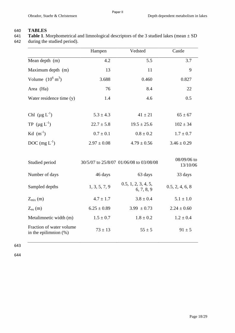
Obrador, Staehr & Christensen Depth dependent metabolism in lakes

Page 18/29

TABLES 640 Table 1. Morphometrical and limnological descriptors of the 3 studied lakes (mean ± SD 641

during the studied period). 642

Hampen Vedsted Castle

Mean depth (m) 4.2 5.5 3.7

Maximum depth (m) 13 11 9

Volume (106 m

3) 3.688 0.460 0.827

Area (Ha) 76 8.4 22

Water residence time (y) 1.4 4.6 0.5

Chl (µg L-1

) 5.3 ± 4.3 41 ± 21 65 ± 67

TP (µg L-1

) 22.7 ± 5.8 19.5 ± 25.6 102 ± 34

Kd (m-1

) 0.7 ± 0.1 0.8 ± 0.2 1.7 ± 0.7

DOC (mg L-1

) 2.97 ± 0.08 4.79 ± 0.56 3.46 ± 0.29

Studied period 30/5/07 to 25/8/07 01/06/08 to 03/08/08 08/09/06 to

13/10/06

Number of days 46 days 63 days 33 days

Sampled depths 1, 3, 5, 7, 9 0.5, 1, 2, 3, 4, 5,

6, 7, 8, 9 0.5, 2, 4, 6, 8

Zmix (m) 4.7 ± 1.7 3.8 ± 0.4 5.1 ± 1.0

Zeu (m) 6.25 ± 0.89 3.99 ± 0.73 2.24 ± 0.60

Metalimnetic width (m) 1.5 ± 0.7 1.8 ± 0.2 1.2 ± 0.4

Fraction of water volume

in the epilimnion (%) 73 ± 13 55 ± 5 91 ± 5

643

644

Paper II

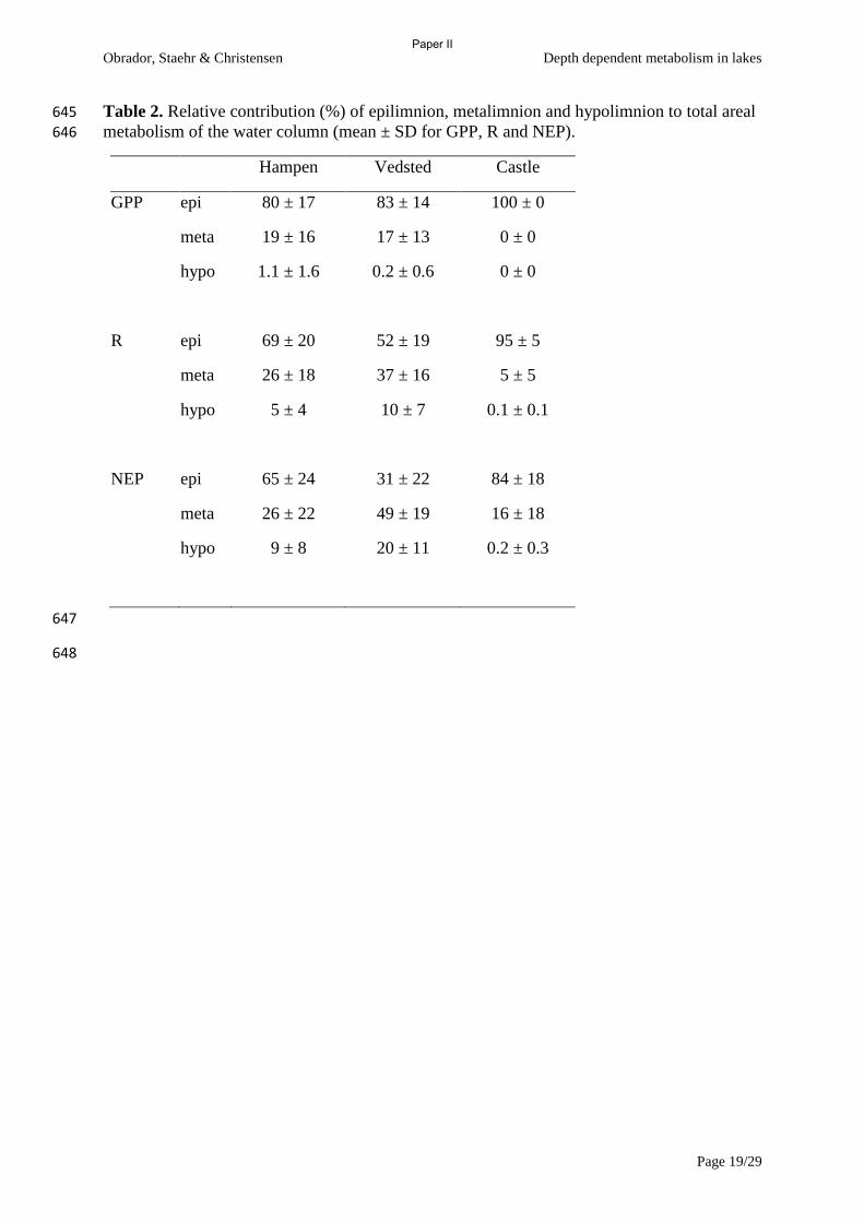
Obrador, Staehr & Christensen Depth dependent metabolism in lakes

Page 19/29

Table 2. Relative contribution (%) of epilimnion, metalimnion and hypolimnion to total areal 645

metabolism of the water column (mean ± SD for GPP, R and NEP). 646

Hampen Vedsted Castle

GPP epi 80 ± 17 83 ± 14 100 ± 0

meta 19 ± 16 17 ± 13 0 ± 0

hypo 1.1 ± 1.6 0.2 ± 0.6 0 ± 0

R epi 69 ± 20 52 ± 19 95 ± 5

meta 26 ± 18 37 ± 16 5 ± 5

hypo 5 ± 4 10 ± 7 0.1 ± 0.1

NEP epi 65 ± 24 31 ± 22 84 ± 18

meta 26 ± 22 49 ± 19 16 ± 18

hypo 9 ± 8 20 ± 11 0.2 ± 0.3

647

648

Paper II

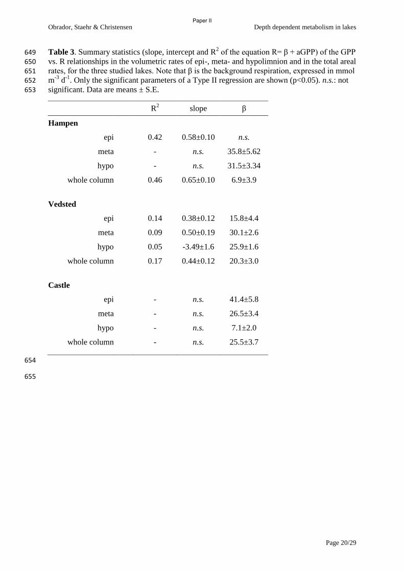
Obrador, Staehr & Christensen Depth dependent metabolism in lakes

Page 20/29

Table 3. Summary statistics (slope, intercept and R2 of the equation R= β + aGPP) of the GPP 649

vs. R relationships in the volumetric rates of epi-, meta- and hypolimnion and in the total areal 650 rates, for the three studied lakes. Note that β is the background respiration, expressed in mmol 651 m

-3 d

-1. Only the significant parameters of a Type II regression are shown (p<0.05). n.s.: not 652

significant. Data are means ± S.E. 653

R2 slope β

Hampen

epi 0.42 0.58±0.10 n.s.

meta - n.s. 35.8±5.62

hypo - n.s. 31.5±3.34

whole column 0.46 0.65±0.10 6.9±3.9

Vedsted

epi 0.14 0.38±0.12 15.8±4.4

meta 0.09 0.50±0.19 30.1±2.6

hypo 0.05 -3.49±1.6 25.9±1.6

whole column 0.17 0.44±0.12 20.3±3.0

Castle

epi - n.s. 41.4±5.8

meta - n.s. 26.5±3.4

hypo - n.s. 7.1±2.0

whole column - n.s. 25.5±3.7

654

655

Paper II

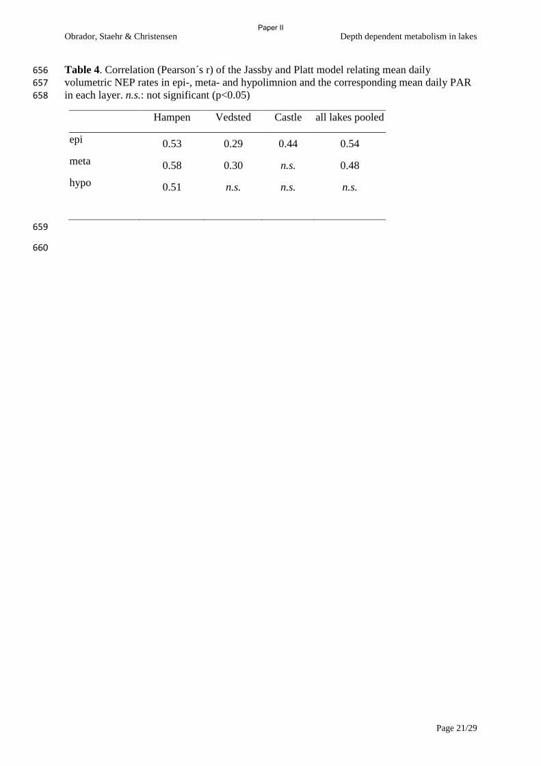
Obrador, Staehr & Christensen Depth dependent metabolism in lakes

Page 21/29

Table 4. Correlation (Pearson´s r) of the Jassby and Platt model relating mean daily 656

volumetric NEP rates in epi-, meta- and hypolimnion and the corresponding mean daily PAR 657

in each layer. n.s.: not significant (p<0.05) 658

Hampen Vedsted Castle all lakes pooled

epi 0.53 0.29 0.44 0.54

meta 0.58 0.30 n.s. 0.48

hypo 0.51 n.s. n.s. n.s.

659

660

Paper II

Obrador, Staehr & Christensen Depth dependent metabolism in lakes

Page 22/29

FIGURE LEGENDS 661

Figure 1. Seasonal variation in the physical structure of the water column and the depth of the 662 photic zone (Zeu, 1% of surface irradiance). Horizontal bars identify the studied periods in 663

each lake. 664

Figure 2. Depth specific daily rates (mmol O2 m-3

d-1

) of gross primary production (GPP). 665 respiration (R), and net ecosystem production (NEP) in Hampen(A-C), Vedsted (D-F) and 666 Castle Lake (H-J). The upper and lower limits of the metalimnetic zone are shown as solid 667 white lines and depth of the photic zone is shown as a dotted line. Time is shown as day of 668

year (DOY) which is not the same for the three lakes (see Table 1). 669

Figure 3. Depth profiles of specific NEP, GPP and R (mmol m-3

d-1

) for the three studied 670 lakes (mean ± SD). The depths of the metalimnion (grey) and of the photic zone (green) are 671 shown on the left boxes through a shading gradation that represents the frequency of a given 672 depth of being within the metalimnion or the photic zone respectively (the horizontal lines 673

there correspond to the 90% confidence interval). 674

Figure 4. Mean areal rates (GPP, R and NEP, in mmol m-2

d-1

) of the depth layers (coloured 675 bars) and integrated whole-column rates (circles) for the three studied lakes. The estimates 676

derived from single-sonde (1m depth) measurements are also shown (triangles). 677

Figure 5. Median and 25th, 75th percentile boxes with 10th, 90th percentile whiskers of GPP 678 (mmol O2 m

-3 d

-1) for the epi-, meta, and hypolimnion of Hampen lake depending on whether 679

the layers are or not in the photic zone. Dots are outliers and the lower case letters denotes the 680 different groups according to Tukey post test. Hypolimnion data was left out of the analysis 681

while they did not pass the test of variance homogeneity. 682

Figure 6. Relationship between daily specific NEP (mmol m-3

d-1

) and mean daily available 683 PAR in each depth layer. The line corresponds to the fitted model at a daily scale, pooling the 684

three lakes (see Table 4). 685

Figure 7. Relative contribution of epilimnetic metabolism to whole-column areal GPP and R 686

in relation with the ratio Zmix : Zeu. The lines correspond to a fitted hyperbolic function with 687

95% confidence intervals (dotted). 688

689

Paper II

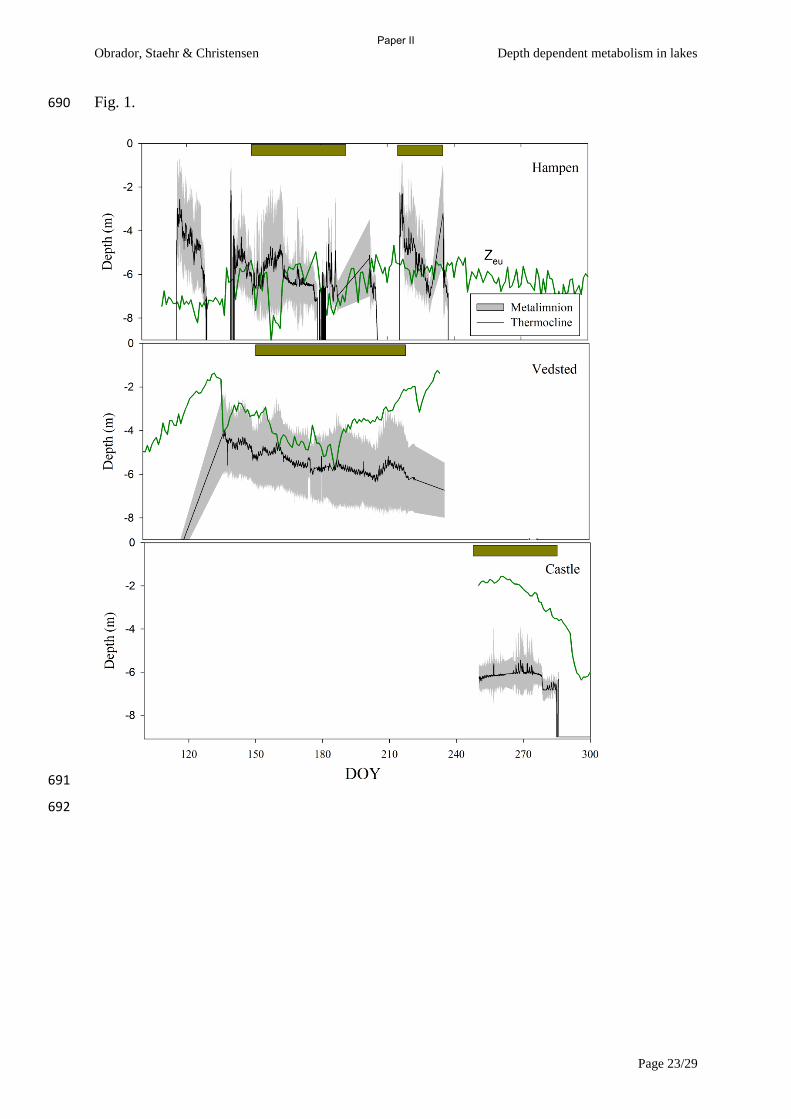
Obrador, Staehr & Christensen Depth dependent metabolism in lakes

Page 23/29

Fig. 1. 690

691

692

Paper II

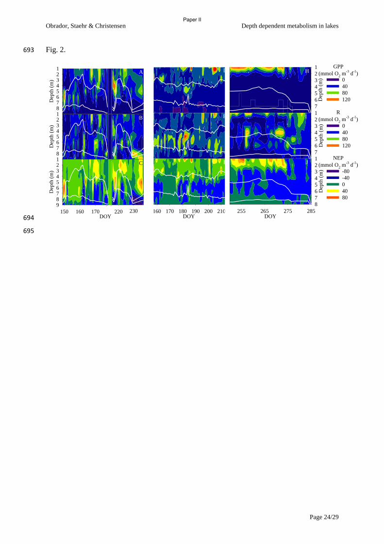
Obrador, Staehr & Christensen Depth dependent metabolism in lakes

Page 24/29

Fig. 2. 693

694

695

160 170 180 190 200 210DOY

D

E

F

Dep

th (

m)

123456789

DOY150 160 170 220

Dep

th (

m)

12345678

Dep

th (

m)

12345678

230

A

B

C

Dep

th (

m)

1

2

3

4

5

6

7

0

40

80

120

255 265 275 285

Dep

th (

m)

1

2

3

4

5

6

7

8

-80

-40

0

40

80

DOY

Dep

th (

m)

1

2

3

4

5

6

7

0

40

80

120

GPP

(mmol O2 m

-3 d

-1)

R

(mmol O2 m

-3 d

-1)

NEP

(mmol O2 m

-3 d

-1)

H

I

J

Paper II

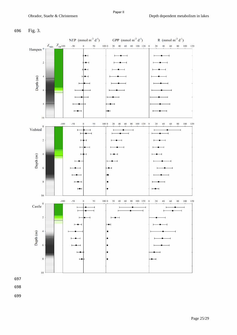
Obrador, Staehr & Christensen Depth dependent metabolism in lakes

Page 25/29

Fig. 3. 696

697

698

699

Paper II

Obrador, Staehr & Christensen Depth dependent metabolism in lakes

Page 26/29

Fig. 4. 700

701

702

Paper II

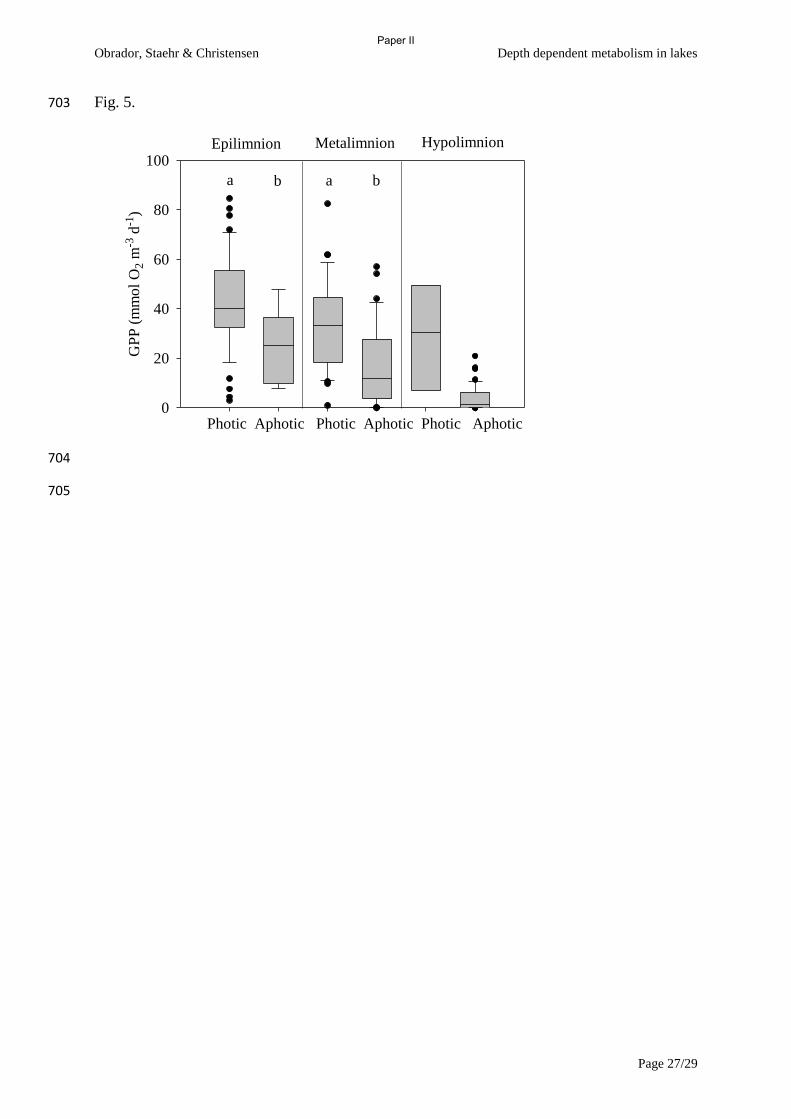
Obrador, Staehr & Christensen Depth dependent metabolism in lakes

Page 27/29

Fig. 5. 703

704

705

a

E PhotE AphotM PhotM AphotH PhotH Aphot

GP

P (

mm

ol

O2 m

-3 d

-1)

0

20

40

60

80

100

ab b

Epilimnion HypolimnionMetalimnion

Photic Aphotic Photic Aphotic Photic Aphotic

Paper II

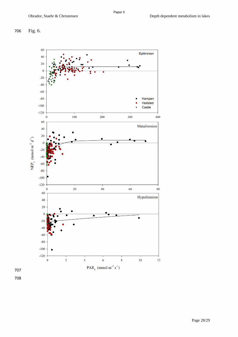
Obrador, Staehr & Christensen Depth dependent metabolism in lakes

Page 28/29

Fig. 6. 706

707

708

Paper II

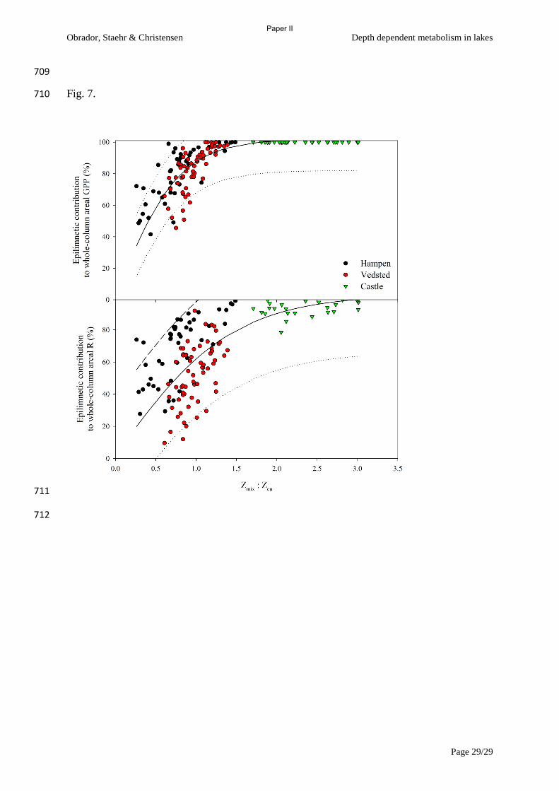
Obrador, Staehr & Christensen Depth dependent metabolism in lakes

Page 29/29

709

Fig. 7. 710

711

712

Paper II

68

Paper III

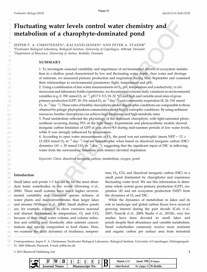
Fluctuating water levels control water chemistry andmetabolism of a charophyte-dominated pond

JESPER P. A. CHRISTENSEN*, KAJ SAND-JENSEN* AND PETER A. STAEHR†

*Freshwater Biological Laboratory, Biological Institute, University of Copenhagen, Hillerød, Denmark†Department of Bioscience, University of Aarhus, Roskilde, Denmark

SUMMARY

1. To investigate seasonal variability and importance of environmental drivers of ecosystem metabo-

lism in a shallow pond characterised by low and fluctuating water depth, clear water and shortage

of nutrients, we measured primary production and respiration during May–September and examined

their relationships to environmental parameters (light, temperature and pH).

2. Using a combination of free watermeasurements of O2, pH, temperature and conductivity, in situ

mesocosm and laboratory bottle experiments, we documented extreme daily variations in environmental

variables (e.g. 0–700 mmol O2 m�3, pH 7.5–9.5, 18–32 °C) and high and variable areal rates of gross

primary production (GPP, 30–316 mmol O2 m�2 day�1) and community respiration (R, 26–318 mmol

O2 m�2 day�1). These rates of benthic charophytes under oligotrophic conditions are comparable to those

obtained by pelagic phytoplankton communities under highly eutrophic conditions. By using sediment

resources, benthic charophytes can achieve high biomasses and highmetabolic rates.

3. Pond metabolism reflected the physiology of the dominant charophyte, with light-saturated photo-

synthesis occurring during 55% of the light hours. Experiments and photosynthetic models showed

inorganic carbon limitation of GPP at pHs above 9.5 during mid-summer periods of low water levels,

while R was strongly influenced by temperature.

4. According to open water measurements of O2, the pond was net autotrophic (mean NEP = 12 �13 (SD) mmol O2 m�2 day�1) but net heterotrophic when based on dissolved inorganic carbon (DIC)

dynamics (10 � 29 mmol CO2 m�2 day�1), suggesting that the significant input of DIC in inflowing

water from the surrounding limestone soils mimics elevated respiration.

Keywords: Chara, dissolved inorganic carbon, metabolism, oxygen, pond

Introduction

Small lakes and ponds (<1 ha) are by far the most abun-

dant lentic waterbodies in the world (Downing et al.,

2006). These small systems have much higher environ-

mental variability and combined species richness of

water plants and macroinvertebrates than larger lakes

and streams (Williams et al., 2004). Small shallow ponds

are, for example, expected to show extensive seasonal

and diurnal fluctuations in temperature, O2 and CO2

because of their small water volume, and volume reduc-

tion and refilling may drastically alter nutrient concen-

trations and species composition in food chains. Here,

we examine the daily dynamics of irradiance, tempera-

ture, O2, CO2 and dissolved inorganic carbon (DIC) in a

small pond dominated by charophytes and experience

fluctuating water level. We use this information to deter-

mine whole system gross primary production (GPP), res-

piration (R) and net ecosystem production (NEP) from

the dynamics of O2 and DIC.

While the dynamics of metabolism in lakes and its

role in landscape and global carbon fluxes have received

growing interest during the past decade (Cole et al.,

2007; Tranvik et al., 2009; Staehr et al., 2012b), very few

studies have been devoted to small lakes and

ponds despite their abundance and variable metabolism.

Small waterbodies commonly receive more nutrients

and organic carbon per surface area from terrestrial

Correspondence: Jesper P. A. Christensen, Freshwater Biological Laboratory, Biological Institute, University of Copenhagen, Helsingørsgade

51, 3400 Hillerød, Denmark. E-mail: jc@bio.ku.dk

1

2

3

4

5

6

7

8

9

10

11

12

13

14

15

16

17

18

19

20

21

22

23

24

25

26

27

28

29

30

31

32

33

34

35

36

37

38

39

40

41

42

43

44

45

46

47

48

49

50

51

© 2013 Blackwell Publishing Ltd 1

Freshwater Biology (2013) doi:10.1111/fwb.12132

F W B 1 2 1 3 2 B Dispatch: 4.3.13 Journal: FWB CE: Suganya

Journal Name Manuscript No. Author Received: No. of pages: 13 PE: Kiruthika

Paper III

surroundings than large lakes. Therefore, they often sup-

port high rates of photosynthesis and even higher rates

of community respiration, leading to profound net het-

erotrophy and CO2 evasion to the atmosphere (Sand-

Jensen & Staehr, 2009). In open nutrient-poor land-

scapes, ponds and shallow lakes may support dense

growths of benthic plants and experience highly variable

water levels and therefore behave very differently than

larger, deeper lakes. Thus, it is possible that net autotro-

phy prevails during water-filled periods of active plant

growth in transparent ponds, while net heterotrophy

prevails during volume reduction because accompany-

ing higher temperatures may stimulate respiration more

than photosynthesis (Staehr & Sand-Jensen, 2006). Com-

plete desiccation, die-off of aquatic benthic plants and

subsequent refilling of ponds could release nutrients

and restart growth of benthic vegetation (Boulton &

Brock, 1999; Arle, 2002). Here, we focus on changes in

metabolism during a fourfold to fivefold change in sur-

face area and water volume due to volume reduction

and refilling of a small pond. The pond is dominated by

charophytes, and it is located on the ultra-oligotrophic

limestone Alvar on €Oland in south-east Sweden.

Summer evaporation in ponds may reduce the water

volume appreciably (Williams, 1985) and enhance diur-

nal changes in temperature, O2, pH and CO2. High O2

and low CO2 concentrations generated by photosynthe-

sis of dense benthic vegetation can restrict further photo-

synthesis and growth by inducing inorganic carbon

limitation and increasing photorespiration (Van, Haller

& Bowes, 1976). Charophytes can directly reduce DIC by

ordinary use of CO2 or HCO�3 coupled with CaCO3 pre-

cipitation on the cell surface and CO2 assimilation into

organic matter during photosynthesis according to the

processes: Ca2+ + 2 HCO�3 ? CaCO3 + CO2 + H2O and

CO2 + H2O ?CH2O (organic matter) + O2 (McConn-

aughey, 1991). Photosynthesis with carbonate precipita-

tion has no or little direct impact on pH, since the

process generates H+ for CO2 formation from HCO�3 .

When the coupled carbonate precipitation and CO2

assimilation operate efficiently in charophytes, they may

be less restricted by high pH than less-efficient algae

and vascular plants (Kufel & Kufel, 2002). However, a

certain reduction in photosynthesis is anticipated

because CO2 is preferred relative to HCO�3 (Maberly &

Madsen, 2002). Photosynthetic use of CO2 or HCO�3uncoupled from carbonate precipitation on the cell sur-

face drives pH upwards more rapidly and may enhance

photosynthetic limitation. We here test the influence of

pH and CO2 on photosynthesis of charophytes in field

mesocosms and laboratory experiments.

Elevated pH during summer generated by intense

photosynthesis in shallow systems may also inhibit bac-

terial respiration and hence carbon mineralisation as

demonstrated by pH manipulation of bacterioplankton

in mesocosms (Tank, Lesack & Mcqueen, 2009). If this

pH-inhibition of community respiration is stronger than

inhibition of gross photosynthesis, it could lead to

higher net autotrophy at least on a short-term basis. We

here test whether pH-inhibition of respiration also takes

place in the field by elevating pH to 9.5.

Our overall hypothesis is that metabolism in shallow

ponds is not easily comparable with that of larger lakes

described by previous studies because ponds are under

stronger influence by environmental drivers (e.g. water

volume, temperature, O2, DIC and CO2). As a result of

shallow water and restricted phytoplankton growth

under nutrient limitation in the studied shallow pond,

we expect that benthic photosynthesis will be light-satu-

rated during most of the day in contrast to what has

previously been found in deeper or more turbid lakes

(Hanson et al., 2008). More specifically we hypothesise

that (i) diurnal variations in temperature, oxygen, pH,

DIC and metabolic rates per volume will be very exten-

sive in the shallow pond, (ii) volume reduction will

increase environmental variability and induce profound

changes in metabolism, and (iii) both photosynthesis

and respiration will be constrained by high pH gener-

ated by dense plant communities in small water

volumes. To investigate these hypotheses, we made con-

tinuous measurements of O2, pH, temperature and con-

ductivity for four summer months and conducted

controlled experiments in field mesocosms and in the

laboratory to investigate the response of plant metabo-

lism to temperature, pH and light.

Methods

Study site and lake characteristics

The study was conducted from May to September 2010

in a small pond in a limestone quarry abandoned

30 years ago on R€applinge Alvar, €Oland, south-east

Sweden (56.8113°N 16.6085°E). Pond area varied from

700 to 3400 m2 and maximum depth from 0.3 to 0.8 m.

Water depth was measured continuously at the deepest

site by recording pressure differences between a sub-

merged HOBO U 20 water level data logger and a simi-

lar logger in air. Water volume ranged between 120 and

1200 m3 according to the recorded water level and mea-

surements of water depth in a grid of 215 measurements

across the lake surface. A 6th-order polynomial equation

© 2013 Blackwell Publishing Ltd, Freshwater Biology, doi: 10.1111/fwb.12132

2 J. P. A. Christensen et al.

1

2

3

4

5

6

7

8

9

10

11

12

13

14

15

16

17

18

19

20

21

22

23

24

25

26

27

28

29

30

31

32

33

34

35

36

37

38

39

40

41

42

43

44

45

46

47

48

49

50

51

Paper III

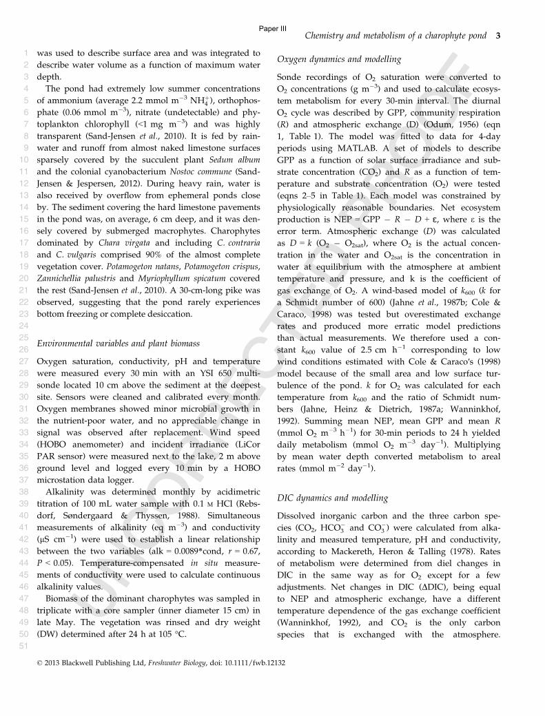
was used to describe surface area and was integrated to

describe water volume as a function of maximum water

depth.

The pond had extremely low summer concentrations

of ammonium (average 2.2 mmol m�3 NHþ4 ), orthophos-

phate (0.06 mmol m�3), nitrate (undetectable) and phy-

toplankton chlorophyll (<1 mg m�3) and was highly

transparent (Sand-Jensen et al., 2010). It is fed by rain-

water and runoff from almost naked limestone surfaces

sparsely covered by the succulent plant Sedum album

and the colonial cyanobacterium Nostoc commune (Sand-

Jensen & Jespersen, 2012). During heavy rain, water is

also received by overflow from ephemeral ponds close

by. The sediment covering the hard limestone pavements

in the pond was, on average, 6 cm deep, and it was den-

sely covered by submerged macrophytes. Charophytes

dominated by Chara virgata and including C. contraria

and C. vulgaris comprised 90% of the almost complete

vegetation cover. Potamogeton natans, Potamogeton crispus,

Zannichellia palustris and Myriophyllum spicatum covered

the rest (Sand-Jensen et al., 2010). A 30-cm-long pike was

observed, suggesting that the pond rarely experiences

bottom freezing or complete desiccation.

Environmental variables and plant biomass

Oxygen saturation, conductivity, pH and temperature

were measured every 30 min with an YSI 650 multi-

sonde located 10 cm above the sediment at the deepest

site. Sensors were cleaned and calibrated every month.

Oxygen membranes showed minor microbial growth in

the nutrient-poor water, and no appreciable change in

signal was observed after replacement. Wind speed

(HOBO anemometer) and incident irradiance (LiCor

PAR sensor) were measured next to the lake, 2 m above

ground level and logged every 10 min by a HOBO

microstation data logger.

Alkalinity was determined monthly by acidimetric

titration of 100 mL water sample with 0.1 M HCl (Rebs-

dorf, Søndergaard & Thyssen, 1988). Simultaneous

measurements of alkalinity (eq m�3) and conductivity

(lS cm�1) were used to establish a linear relationship

between the two variables (alk = 0.0089*cond, r = 0.67,

P < 0.05). Temperature-compensated in situ measure-

ments of conductivity were used to calculate continuous

alkalinity values.

Biomass of the dominant charophytes was sampled in

triplicate with a core sampler (inner diameter 15 cm) in

late May. The vegetation was rinsed and dry weight

(DW) determined after 24 h at 105 °C.

Oxygen dynamics and modelling

Sonde recordings of O2 saturation were converted to

O2 concentrations (g m�3) and used to calculate ecosys-

tem metabolism for every 30-min interval. The diurnal

O2 cycle was described by GPP, community respiration

(R) and atmospheric exchange (D) (Odum, 1956) (eqn

1, Table 1). The model was fitted to data for 4-day

periods using MATLAB. A set of models to describe

GPP as a function of solar surface irradiance and sub-

strate concentration (CO2) and R as a function of tem-

perature and substrate concentration (O2) were tested

(eqns 2–5 in Table 1). Each model was constrained by

physiologically reasonable boundaries. Net ecosystem

production is NEP = GPP � R � D + ɛ, where e is the

error term. Atmospheric exchange (D) was calculated

as D = k (O2 � O2sat), where O2 is the actual concen-

tration in the water and O2sat is the concentration in

water at equilibrium with the atmosphere at ambient

temperature and pressure, and k is the coefficient of

gas exchange of O2. A wind-based model of k600 (k for

a Schmidt number of 600) (Jahne et al., 1987b; Cole &

Caraco, 1998) was tested but overestimated exchange

rates and produced more erratic model predictions

than actual measurements. We therefore used a con-

stant k600 value of 2.5 cm h�1 corresponding to low

wind conditions estimated with Cole & Caraco′s (1998)

model because of the small area and low surface tur-

bulence of the pond. k for O2 was calculated for each

temperature from k600 and the ratio of Schmidt num-

bers (Jahne, Heinz & Dietrich, 1987a; Wanninkhof,

1992). Summing mean NEP, mean GPP and mean R

(mmol O2 m�3 h�1) for 30-min periods to 24 h yielded

daily metabolism (mmol O2 m�3 day�1). Multiplying

by mean water depth converted metabolism to areal

rates (mmol m�2 day�1).

DIC dynamics and modelling

Dissolved inorganic carbon and the three carbon spe-

cies (CO2, HCO�3 and CO�3 ) were calculated from alka-

linity and measured temperature, pH and conductivity,

according to Mackereth, Heron & Talling (1978). Rates

of metabolism were determined from diel changes in

DIC in the same way as for O2 except for a few

adjustments. Net changes in DIC (DDIC), being equal

to NEP and atmospheric exchange, have a different

temperature dependence of the gas exchange coefficient

(Wanninkhof, 1992), and CO2 is the only carbon

species that is exchanged with the atmosphere.

© 2013 Blackwell Publishing Ltd, Freshwater Biology, doi: 10.1111/fwb.12132

Chemistry and metabolism of a charophyte pond 3

1

2

3

4

5

6

7

8

9

10

11

12

13

14

15

16

17

18

19

20

21

22

23

24

25

26

27

28

29

30

31

32

33

34

35

36

37

38

39

40

41

42

43

44

45

46

47

48

49

50

51

Paper III

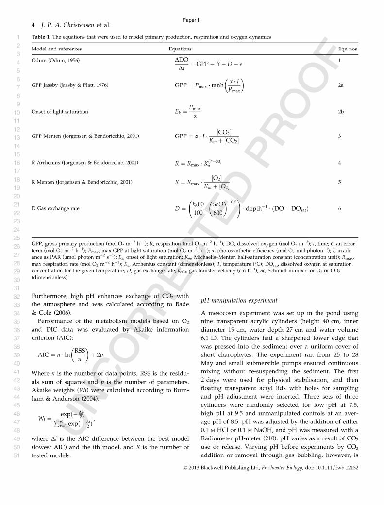
Furthermore, high pH enhances exchange of CO2 with

the atmosphere and was calculated according to Bade

& Cole (2006).

Performance of the metabolism models based on O2

and DIC data was evaluated by Akaike information

criterion (AIC):

AIC ¼ n � ln RSS

n

� �

þ 2p

Where n is the number of data points, RSS is the residu-

als sum of squares and p is the number of parameters.

Akaike weights (Wi) were calculated according to Burn-

ham & Anderson (2004).

Wi ¼expð� Di

2 ÞPR

r¼1 expð� Di2 Þ;

where Di is the AIC difference between the best model

(lowest AIC) and the ith model, and R is the number of

tested models.

pH manipulation experiment

A mesocosm experiment was set up in the pond using

nine transparent acrylic cylinders (height 40 cm, inner

diameter 19 cm, water depth 27 cm and water volume

6.1 L). The cylinders had a sharpened lower edge that

was pressed into the sediment over a uniform cover of

short charophytes. The experiment ran from 25 to 28

May and small submersible pumps ensured continuous

mixing without re-suspending the sediment. The first

2 days were used for physical stabilisation, and then

floating transparent acryl lids with holes for sampling

and pH adjustment were inserted. Three sets of three

cylinders were randomly selected for low pH at 7.5,

high pH at 9.5 and unmanipulated controls at an aver-

age pH of 8.5. pH was adjusted by the addition of either

0.1 M HCl or 0.1 M NaOH, and pH was measured with a

Radiometer pH-meter (210). pH varies as a result of CO2

use or release. Varying pH before experiments by CO2

addition or removal through gas bubbling, however, is

Table 1 The equations that were used to model primary production, respiration and oxygen dynamics

Model and references Equations Eqn nos.

Odum (Odum, 1956) DDO

Dt¼ GPP� R�D� � 1

GPP Jassby (Jassby & Platt, 1976) GPP ¼ Pmax � tanha � IPmax

� �

2a

Onset of light saturation Ek ¼Pmax

a2b

GPP Menten (Jorgensen & Bendoricchio, 2001) GPP ¼ a � I � CO2½ �Km þ CO2½ �

3

R Arrhenius (Jorgensen & Bendoricchio, 2001) R ¼ Rmax � K T�30ð Þa

4

R Menten (Jorgensen & Bendoricchio, 2001) R ¼ Rmax �O2½ �

Km þ O2½ �5

D Gas exchange rate D ¼ k600

100� ScO

600

� ��0:5 !

� depth�1 � DO�DOsatð Þ 6

GPP, gross primary production (mol O2 m�2 h�1); R, respiration (mol O2 m

�2 h�1); DO, dissolved oxygen (mol O2 m�2); t, time; ɛ, an error

term (mol O2 m�2 h�1); Pmax, max GPP at light saturation (mol O2 m�2 h�1); a, photosynthetic efficiency (mol O2 mol photon�1); I, irradi-

ance as PAR (lmol photon m�2 s�1); Ek, onset of light saturation; Km, Michaelis–Menten half-saturation constant (concentration unit); Rmax,

max respiration rate (mol O2 m�2 h�1); Ka, Arrhenius constant (dimensionless); T, temperature (°C); DOsat, dissolved oxygen at saturation

concentration for the given temperature; D, gas exchange rate; k600, gas transfer velocity (cm h�1); Sc, Schmidt number for O2 or CO2

(dimensionless).

© 2013 Blackwell Publishing Ltd, Freshwater Biology, doi: 10.1111/fwb.12132

4 J. P. A. Christensen et al.

1

2

3

4

5

6

7

8

9

10

11

12

13

14

15

16

17

18

19

20

21

22

23

24

25

26

27

28

29

30

31

32

33

34

35

36

37

38

39

40

41

42

43

44

45

46

47

48

49

50

51

Paper III

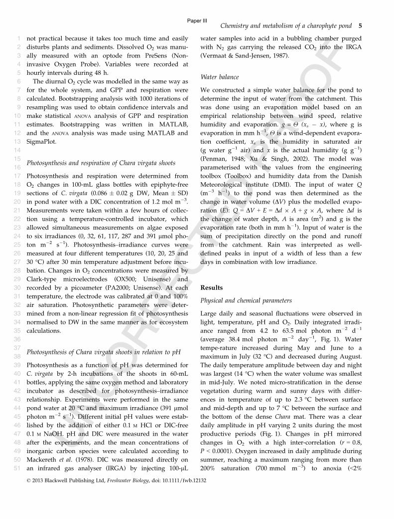
not practical because it takes too much time and easily

disturbs plants and sediments. Dissolved O2 was manu-

ally measured with an optode from PreSens (Non-

invasive Oxygen Probe). Variables were recorded at

hourly intervals during 48 h.

The diurnal O2 cycle was modelled in the same way as

for the whole system, and GPP and respiration were

calculated. Bootstrapping analysis with 1000 iterations of

resampling was used to obtain confidence intervals and

make statistical ANOVA analysis of GPP and respiration

estimates. Bootstrapping was written in MATLAB,

and the ANOVA analysis was made using MATLAB and

SigmaPlot.

Photosynthesis and respiration of Chara virgata shoots

Photosynthesis and respiration were determined from

O2 changes in 100-mL glass bottles with epiphyte-free

sections of C. virgata (0.086 � 0.02 g DW, Mean � SD)

in pond water with a DIC concentration of 1.2 mol m�3.

Measurements were taken within a few hours of collec-

tion using a temperature-controlled incubator, which

allowed simultaneous measurements on algae exposed

to six irradiances (0, 32, 61, 117, 287 and 391 lmol pho-

ton m�2 s�1). Photosynthesis–irradiance curves were

measured at four different temperatures (10, 20, 25 and

30 °C) after 30 min temperature adjustment before incu-

bation. Changes in O2 concentrations were measured by

Clark-type microelectrodes (OX500; Unisense) and

recorded by a picoameter (PA2000; Unisense). At each

temperature, the electrode was calibrated at 0 and 100%

air saturation. Photosynthetic parameters were deter-

mined from a non-linear regression fit of photosynthesis

normalised to DW in the same manner as for ecosystem

calculations.

Photosynthesis of Chara virgata shoots in relation to pH

Photosynthesis as a function of pH was determined for

C. virgata by 2-h incubations of the shoots in 60-mL

bottles, applying the same oxygen method and laboratory

incubator as described for photosynthesis–irradiance

relationship. Experiments were performed in the same

pond water at 20 °C and maximum irradiance (391 lmol

photon m�2 s�1). Different initial pH values were estab-

lished by the addition of either 0.1 M HCl or DIC-free

0.1 M NaOH. pH and DIC were measured in the water

after the experiments, and the mean concentrations of

inorganic carbon species were calculated according to

Mackereth et al. (1978). DIC was measured directly on

an infrared gas analyser (IRGA) by injecting 100-lL

water samples into acid in a bubbling chamber purged

with N2 gas carrying the released CO2 into the IRGA

(Vermaat & Sand-Jensen, 1987).

Water balance

We constructed a simple water balance for the pond to

determine the input of water from the catchment. This

was done using an evaporation model based on an

empirical relationship between wind speed, relative

humidity and evaporation. g = Θ (xs � x), where g is

evaporation in mm h�1, Θ is a wind-dependent evapora-

tion coefficient, xs is the humidity in saturated air

(g water g�1 air) and x is the actual humidity (g g�1)

(Penman, 1948; Xu & Singh, 2002). The model was

parameterised with the values from the engineering

toolbox (Toolbox) and humidity data from the Danish

Meteorological institute (DMI). The input of water Q

(m�3 h�1) to the pond was then determined as the

change in water volume (DV) plus the modelled evapo-

ration (E): Q = DV + E = Dd 9 A + g 9 A, where Dd is

the change of water depth, A is area (m2) and g is the

evaporation rate (both in mm h�1). Input of water is the

sum of precipitation directly on the pond and runoff

from the catchment. Rain was interpreted as well-

defined peaks in input of a width of less than a few

days in combination with low irradiance.

Results

Physical and chemical parameters

Large daily and seasonal fluctuations were observed in

light, temperature, pH and O2. Daily integrated irradi-

ance ranged from 4.2 to 63.5 mol photon m�2 d�1

(average 38.4 mol photon m�2 day�1, Fig. 1). Water

tempe-rature increased during May and June to a

maximum in July (32 °C) and decreased during August.

The daily temperature amplitude between day and night

was largest (14 °C) when the water volume was smallest

in mid-July. We noted micro-stratification in the dense

vegetation during warm and sunny days with differ-

ences in temperature of up to 2.3 °C between surface

and mid-depth and up to 7 °C between the surface and

the bottom of the dense Chara mat. There was a clear

daily amplitude in pH varying 2 units during the most

productive periods (Fig. 1). Changes in pH mirrored

changes in O2 with a high inter-correlation (r = 0.8,

P < 0.0001). Oxygen increased in daily amplitude during

summer, reaching a maximum ranging from more than

200% saturation (700 mmol m�3) to anoxia (<2%

© 2013 Blackwell Publishing Ltd, Freshwater Biology, doi: 10.1111/fwb.12132

Chemistry and metabolism of a charophyte pond 5

1

2

3

4

5

6

7

8

9

10

11

12

13

14

15

16

17

18

19

20

21

22

23

24

25

26

27

28

29

30

31

32

33

34

35

36

37

38

39

40

41

42

43

44

45

46

47

48

49

50

51

Paper III

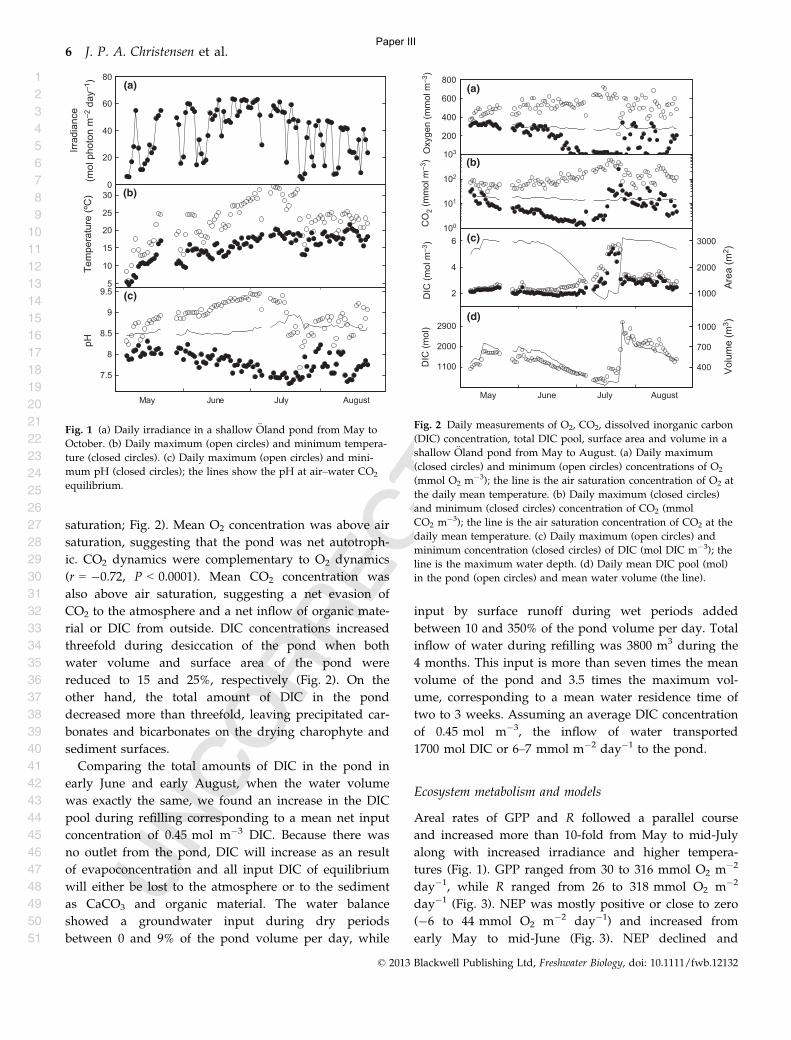
saturation; Fig. 2). Mean O2 concentration was above air

saturation, suggesting that the pond was net autotroph-

ic. CO2 dynamics were complementary to O2 dynamics

(r = �0.72, P < 0.0001). Mean CO2 concentration was

also above air saturation, suggesting a net evasion of

CO2 to the atmosphere and a net inflow of organic mate-

rial or DIC from outside. DIC concentrations increased

threefold during desiccation of the pond when both

water volume and surface area of the pond were

reduced to 15 and 25%, respectively (Fig. 2). On the

other hand, the total amount of DIC in the pond

decreased more than threefold, leaving precipitated car-

bonates and bicarbonates on the drying charophyte and

sediment surfaces.

Comparing the total amounts of DIC in the pond in

early June and early August, when the water volume

was exactly the same, we found an increase in the DIC

pool during refilling corresponding to a mean net input

concentration of 0.45 mol m�3 DIC. Because there was

no outlet from the pond, DIC will increase as an result

of evapoconcentration and all input DIC of equilibrium

will either be lost to the atmosphere or to the sediment

as CaCO3 and organic material. The water balance

showed a groundwater input during dry periods

between 0 and 9% of the pond volume per day, while

input by surface runoff during wet periods added

between 10 and 350% of the pond volume per day. Total

inflow of water during refilling was 3800 m3 during the

4 months. This input is more than seven times the mean

volume of the pond and 3.5 times the maximum vol-

ume, corresponding to a mean water residence time of

two to 3 weeks. Assuming an average DIC concentration

of 0.45 mol m�3, the inflow of water transported

1700 mol DIC or 6–7 mmol m�2 day�1 to the pond.

Ecosystem metabolism and models

Areal rates of GPP and R followed a parallel course

and increased more than 10-fold from May to mid-July

along with increased irradiance and higher tempera-

tures (Fig. 1). GPP ranged from 30 to 316 mmol O2 m�2

day�1, while R ranged from 26 to 318 mmol O2 m�2

day�1 (Fig. 3). NEP was mostly positive or close to zero

(�6 to 44 mmol O2 m�2 day�1) and increased from

early May to mid-June (Fig. 3). NEP declined and

0

20

40

60

80Ir

rad

ian

ce

(mo

l p

ho

ton

m–

2 d

ay

–1)

(a)

5

10

15

20

25

30

Te

mp

era

ture

(ºC

) (b)

7.5

8

8.5

9

9.5 (c)

pH

May June July August

Fig. 1 (a) Daily irradiance in a shallow €Oland pond from May to

October. (b) Daily maximum (open circles) and minimum tempera-

ture (closed circles). (c) Daily maximum (open circles) and mini-

mum pH (closed circles); the lines show the pH at air–water CO2

equilibrium.

200

400

600

800

Oxyg

en

(m

mo

l m

–3)

(a)

100

101

102

103

CO

2 (

mm

ol m

–3) (b)

2

4

6

DIC

(m

ol m

–3) (c)

1100

2000

2900(d)

DIC

(m

ol)

May July AugustJune

1000

2000

3000

Are

a (

m2)

400

700

1000

Vo

lum

e (

m3)

Fig. 2 Daily measurements of O2, CO2, dissolved inorganic carbon

(DIC) concentration, total DIC pool, surface area and volume in a

shallow €Oland pond from May to August. (a) Daily maximum

(closed circles) and minimum (open circles) concentrations of O2

(mmol O2 m�3); the line is the air saturation concentration of O2 at

the daily mean temperature. (b) Daily maximum (closed circles)

and minimum (closed circles) concentration of CO2 (mmol

CO2 m�3); the line is the air saturation concentration of CO2 at the

daily mean temperature. (c) Daily maximum (open circles) and

minimum concentration (closed circles) of DIC (mol DIC m�3); the

line is the maximum water depth. (d) Daily mean DIC pool (mol)

in the pond (open circles) and mean water volume (the line).

© 2013 Blackwell Publishing Ltd, Freshwater Biology, doi: 10.1111/fwb.12132

6 J. P. A. Christensen et al.

1

2

3

4

5

6

7

8

9

10

11

12

13

14

15

16

17

18

19

20

21

22

23

24

25

26

27

28

29

30

31

32

33

34

35

36

37

38

39

40

41

42

43

44

45

46

47

48

49

50

51

Paper III

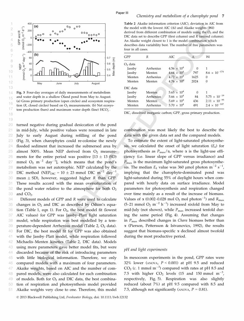
turned negative during gradual desiccation of the pond

in mid-July, while positive values were resumed in late

July to early August during refilling of the pond

(Fig. 3), when charophytes could re-colonise the newly

flooded sediment that increased the submersed area by

almost 500%. Mean NEP derived from O2 measure-

ments for the entire period was positive [13 � 13 (SD)

mmol O2 m�2 day�1], which means that the pond’s

metabolism was net autotrophic. NEP calculated by the

DIC method (NEPDIC = 10 � 23 mmol DIC m�2 day�1

mean � SD), however, suggested higher R than GPP.

These results accord with the mean oversaturation of

the pond water relative to the atmosphere for both O2

and CO2.

Different models of GPP and R were used to calculate

changes in O2 and DIC as described by Odum’s equa-

tion (Table 1, eqn 1). For O2, the best model fit (lowest

AIC values) for GPP was Jassby–Platt light saturation

model, while respiration was best modelled by a tem-

perature-dependent Arrhenius model (Table 2, O2 data).

For DIC, the best model fit for GPP was also obtained

with the Jassby–Platt model, while respiration followed

Michaelis–Menten kinetics (Table 2, DIC data). Models

using more parameters gave better model fits, but were

discarded because of the risk of introducing parameters

with little biological information. Therefore, we only

compared models with a maximum of four parameters.

Akaike weights, based on AIC and the number of com-

pared models, were also calculated for each combination

of models. Both for O2 and DIC data, the best combina-

tion of respiration and photosynthesis model provided

Akaike weights very close to one. Therefore, this model

combination was most likely the best to describe the

data with the given data set and the compared models.

To estimate the extent of light-saturated photosynthe-

sis, we calculated the onset of light saturation (Ek) for

photosynthesis as Pmax/a, where a is the light-use effi-

ciency (i.e. linear slope of GPP versus irradiance) and

Pmax is the maximum light-saturated gross photosynthe-

sis. The median Ek value was 360 lmol photon m�2 s�1,

implying that the charophyte-dominated pond was

light-saturated during 55% of daylight hours when com-

pared with hourly data on surface irradiance. Model

parameters for photosynthesis and respiration changed

over time mainly as a result of the increase of biomass.

Values of a (0.002–0.028 mol O2 mol photon�1) and Rmax

(5–21 mmol O2 m�2 h�1) increased sixfold from May to

mid-July (not shown), while Pmax increased tenfold dur-

ing the same period (Fig. 4). Assuming that changes

in Pmax described changes in Chara biomass better than

a (Pierson, Pettersson & Istvanovics, 1992), the results

suggest that biomass-specific a declined almost twofold

during the most productive period.

pH and light experiments

In mesocosm experiments in the pond, GPP rates were

32% lower (ANOVA, P < 0.001) at pH 9.5 and reduced

CO2 (c. 1 mmol m�3) compared with rates at pH 8.5 and

7.5 with higher CO2 levels (15 and 150 mmol m�3,

respectively, Fig. 5). Respiration was also slightly

reduced (about 7%) at pH 9.5 compared with 8.5 and

7.5, although not significantly (ANOVA, P = 0.81).

–400

–200

0

200

400

GP

P a

nd

R

(mm

ol O

2 m

–2 d

–1) (a)

0

20

40

60

NE

P

(mm

ol O

2 m

–2 d

ay

–1)

May June July August

(b)

0.4

0.5

0.6

0.7

Ma

x d

ep

th (

m)

Fig. 3 Four-day averages of daily measurements of metabolism

and water depth in a shallow €Oland pond from May to August.

(a) Gross primary production (open circles) and ecosystem respira-

tion (R, closed circles) based on O2 measurements. (b) Net ecosys-

tem production (bars) and maximum water depth (line) HCO�3 .

Table 2 Akaike information criterion (AIC), deviation in AIC from

the model with the lowest AIC (Di) and Akaike weights (Wi)

derived from different combination of models using the O2 and the

DIC data set to describe GPP (first column) and R (second column).

An Akaike weight closest to 1 is the model combination which

describes data variability best. The number of free parameters was

four in all cases.

GPP R AIC Di Wi

O2 data

Jassby Arrhenius 4.56 9 104 0 1

Jassby Menten 4.64 9 104 797 8.6 9 10�174

Menten Arrhenius 4.72 9 104 1625 0

Menten Menten 4.76 9 104 2024 0

DIC data

Jassby Menten 5.65 9 104 0 1

Jassby Arrhenius 5.66 9 104 84 5.75 9 10�19

Menten Menten 5.69 9 104 436 2.11 9 10�95

Menten Arrhenius 5.70 9 104 491 2.4 9 10�107

DIC, dissolved inorganic carbon; GPP, gross primary production.

© 2013 Blackwell Publishing Ltd, Freshwater Biology, doi: 10.1111/fwb.12132

Chemistry and metabolism of a charophyte pond 7

1

2

3

4

5

6

7

8

9

10

11

12

13

14

15

16

17

18

19

20

21

22

23

24

25

26

27

28

29

30

31

32

33

34

35

36

37

38

39

40

41

42

43

44

45

46

47

48

49

50

51

Paper III

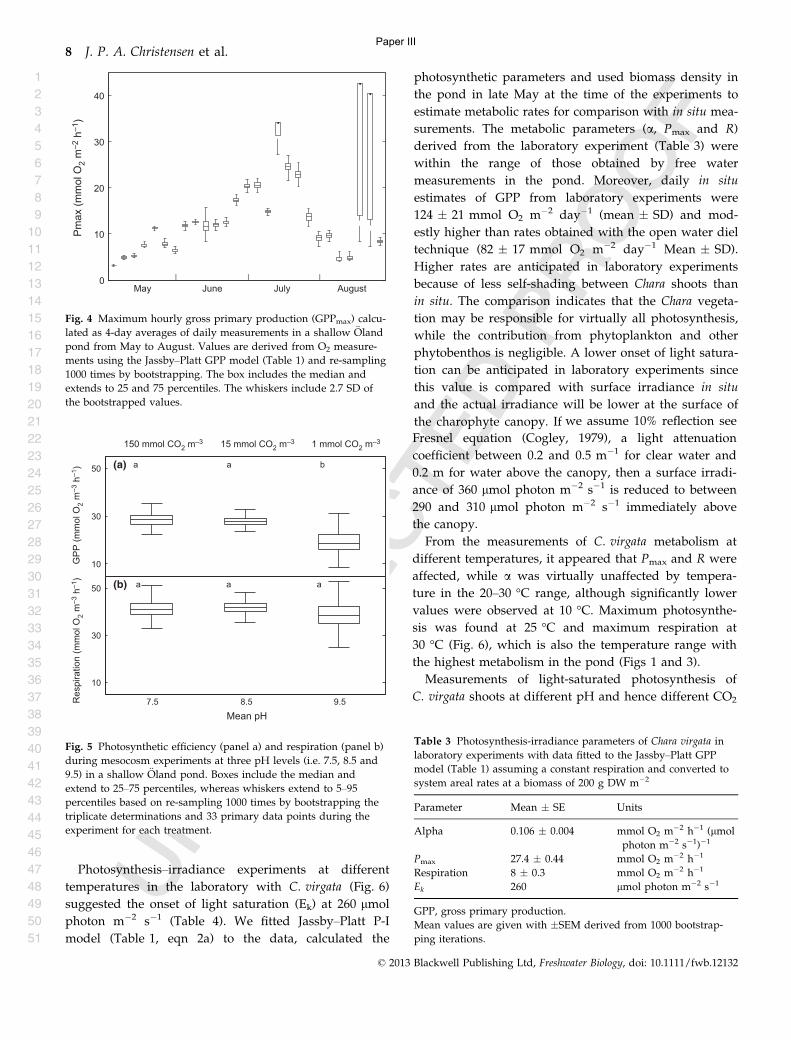
Photosynthesis–irradiance experiments at different

temperatures in the laboratory with C. virgata (Fig. 6)

suggested the onset of light saturation (Ek) at 260 lmol

photon m�2 s�1 (Table 4). We fitted Jassby–Platt P-I

model (Table 1, eqn 2a) to the data, calculated the

photosynthetic parameters and used biomass density in

the pond in late May at the time of the experiments to

estimate metabolic rates for comparison with in situ mea-

surements. The metabolic parameters (a, Pmax and R)

derived from the laboratory experiment (Table 3) were

within the range of those obtained by free water

measurements in the pond. Moreover, daily in situ

estimates of GPP from laboratory experiments were

124 � 21 mmol O2 m�2 day�1 (mean � SD) and mod-

estly higher than rates obtained with the open water diel

technique (82 � 17 mmol O2 m�2 day�1 Mean � SD).

Higher rates are anticipated in laboratory experiments

because of less self-shading between Chara shoots than

in situ. The comparison indicates that the Chara vegeta-

tion may be responsible for virtually all photosynthesis,

while the contribution from phytoplankton and other

phytobenthos is negligible. A lower onset of light satura-

tion can be anticipated in laboratory experiments since

this value is compared with surface irradiance in situ

and the actual irradiance will be lower at the surface of

the charophyte canopy. If 9we assume 10% reflection see

Fresnel equation (Cogley, 1979), a light attenuation

coefficient between 0.2 and 0.5 m�1 for clear water and

0.2 m for water above the canopy, then a surface irradi-

ance of 360 lmol photon m�2 s�1 is reduced to between

290 and 310 lmol photon m�2 s�1 immediately above

the canopy.

From the measurements of C. virgata metabolism at

different temperatures, it appeared that Pmax and R were

affected, while a was virtually unaffected by tempera-

ture in the 20–30 °C range, although significantly lower

values were observed at 10 °C. Maximum photosynthe-

sis was found at 25 °C and maximum respiration at

30 °C (Fig. 6), which is also the temperature range with

the highest metabolism in the pond (Figs 1 and 3).

Measurements of light-saturated photosynthesis of

C. virgata shoots at different pH and hence different CO2

0

10

20

30

40

May June July August

Pm

ax (

mm

ol O

2 m

–2 h

–1)

Fig. 4 Maximum hourly gross primary production (GPPmax) calcu-

lated as 4-day averages of daily measurements in a shallow €Oland

pond from May to August. Values are derived from O2 measure-

ments using the Jassby–Platt GPP model (Table 1) and re-sampling

1000 times by bootstrapping. The box includes the median and

extends to 25 and 75 percentiles. The whiskers include 2.7 SD of

the bootstrapped values.

10

30

50

GP

P (

mm

ol O

2 m

–3 h

–1)

150 mmol CO2 m–3 15 mmol CO2 m–3 1 mmol CO2 m–3

baa(a)

10

30

50

9.58.57.5

Mean pH

Re

sp

ira

tio

n (

mm

ol O

2 m

–3 h

–1)

aaa(b)

Fig. 5 Photosynthetic efficiency (panel a) and respiration (panel b)

during mesocosm experiments at three pH levels (i.e. 7.5, 8.5 and

9.5) in a shallow €Oland pond. Boxes include the median and

extend to 25–75 percentiles, whereas whiskers extend to 5–95

percentiles based on re-sampling 1000 times by bootstrapping the

triplicate determinations and 33 primary data points during the

experiment for each treatment.

Table 3 Photosynthesis-irradiance parameters of Chara virgata in

laboratory experiments with data fitted to the Jassby–Platt GPP

model (Table 1) assuming a constant respiration and converted to

system areal rates at a biomass of 200 g DW m�2

Parameter Mean � SE Units

Alpha 0.106 � 0.004 mmol O2 m�2 h�1 (lmol

photon m�2 s�1)�1

Pmax 27.4 � 0.44 mmol O2 m�2 h�1

Respiration 8 � 0.3 mmol O2 m�2 h�1

Ek 260 lmol photon m�2 s�1

GPP, gross primary production.

Mean values are given with �SEM derived from 1000 bootstrap-

ping iterations.

© 2013 Blackwell Publishing Ltd, Freshwater Biology, doi: 10.1111/fwb.12132

8 J. P. A. Christensen et al.

1

2

3

4

5

6

7

8

9

10

11

12

13

14

15

16

17

18

19

20

21

22

23

24

25

26

27

28

29

30

31

32

33

34

35

36

37

38

39

40

41

42

43

44

45

46

47

48

49

50

51

Paper III

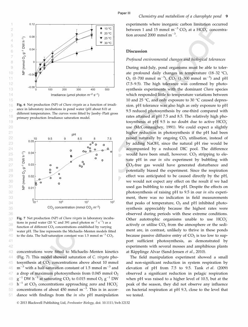
concentrations were fitted to Michaelis–Menten kinetics

(Fig. 7). This model showed saturation of C. virgata pho-

tosynthesis at CO2 concentrations above about 10 mmol

m�3 with a half-saturation constant of 1.5 mmol m�3 and

a drop of maximum photosynthesis from 0.045 mmol O2

g�1 DW h�1 at saturating CO2 to 0.015 mmol O2 g�1 DW

h�1 at CO2 concentrations approaching zero and HCO�3concentrations of about 450 mmol m�3. This is in accor-

dance with findings from the in situ pH manipulation

experiments where inorganic carbon limitation occurred

between 1 and 15 mmol m�3 CO2 at a HCO�3 concentra-

tion around 2000 mmol m�3.

Discussion

Profound environmental changes and biological tolerances

During mid-July, pond organisms must be able to toler-

ate profound daily changes in temperature (18–32 °C),

O2 (0–700 mmol m�3), CO2 (1–300 mmol m�3) and pH

(7.5–9.5). The high tolerance was confirmed by photo-

synthesis experiments with the dominant Chara species

which responded little to temperature variations between

10 and 25 °C, and only exposure to 30 °C caused depres-

sion. pH tolerance was also high as only exposure to pH

9.5 reduced photosynthesis by one-third compared with

rates attained at pH 7.5 and 8.5. The relatively high pho-

tosynthesis at pH 9.5 is no doubt due to active HCO�3use (McConnaughey, 1991). We could expect a slightly

higher reduction in photosynthesis if the pH had been

raised naturally by ongoing CO2 utilisation, instead of

by adding NaOH, since the natural pH rise would be

accompanied by a reduced DIC pool. The difference

would have been small, however. CO2 stripping to ele-

vate pH in our in situ experiment by bubbling with

CO2-free gas would have generated disturbance and

potentially biased the experiment. Since the respiration

effect was anticipated to be caused directly by the pH,

we would not expect any effect on the result if we had

used gas bubbling to raise the pH. Despite the effects on

photosynthesis of raising pH to 9.5 in our in situ experi-

ment, there was no indication in field measurements

that peaks of temperature, O2 and pH inhibited photo-

synthesis appreciably because the highest rates were

observed during periods with these extreme conditions.

Other autotrophic organisms unable to use HCO�3actively or utilise CO2 from the atmosphere or the sedi-

ment are, in contrast, unlikely to thrive in these ponds

because passive diffusive entry of CO2 is too low to sup-

port sufficient photosynthesis, as demonstrated by

experiments with several mosses and amphibious plants

at R€applinge Alvar (Sand-Jensen et al., 2010).

The field manipulation experiment showed a small

and non-significant reduction in system respiration by

elevation of pH from 7.5 to 9.5. Tank et al. (2009)

observed a significant reduction in pelagic respiration

when pH was raised to a higher level of 10.5, but at the

peak of the season, they did not observe any influence

on bacterial respiration at pH 9.3, close to the level that

we tested.

0 100 200 300 400 500–0.08

–0.04

0

0.04

0.08

0.12

Irradiance (µmol photon m–2 s–1)

NP

(m

mo

l O

2 g

–1 D

W h

–1)

10 ºC

20 ºC

25 ºC

30 ºC

Fig. 6 Net production (NP) of Chara virgata as a function of irradi-

ance in laboratory incubations in pond water (pH about 8.0) at

different temperatures. The curves were fitted by Jassby–Platt gross

primary production–Irradiance saturation model.

10–1 100 101 1020

0.01

0.02

0.03

0.04

0.05

NP

(m

mol O

2 g

–1 D

W h

–1)

CO2 concentration (mmol CO2 m–3)

7.588.599.510

pH

Fig. 7 Net production (NP) of Chara virgata in laboratory incuba-

tions in pond water (20 °C and 391 lmol photon m�2 s�1) as a

function of different CO2 concentrations established by varying

water pH. The line represents the Michaelis–Menten models fitted

to the data. The half-saturation constant was 1.5 mmol m�3 CO2.

© 2013 Blackwell Publishing Ltd, Freshwater Biology, doi: 10.1111/fwb.12132

Chemistry and metabolism of a charophyte pond 9

1

2

3

4

5

6

7

8

9

10

11

12

13

14

15

16

17

18

19

20

21

22

23

24

25

26

27

28

29

30

31

32

33

34

35

36

37

38

39

40

41

42

43

44

45

46

47

48

49

50

51

Paper III

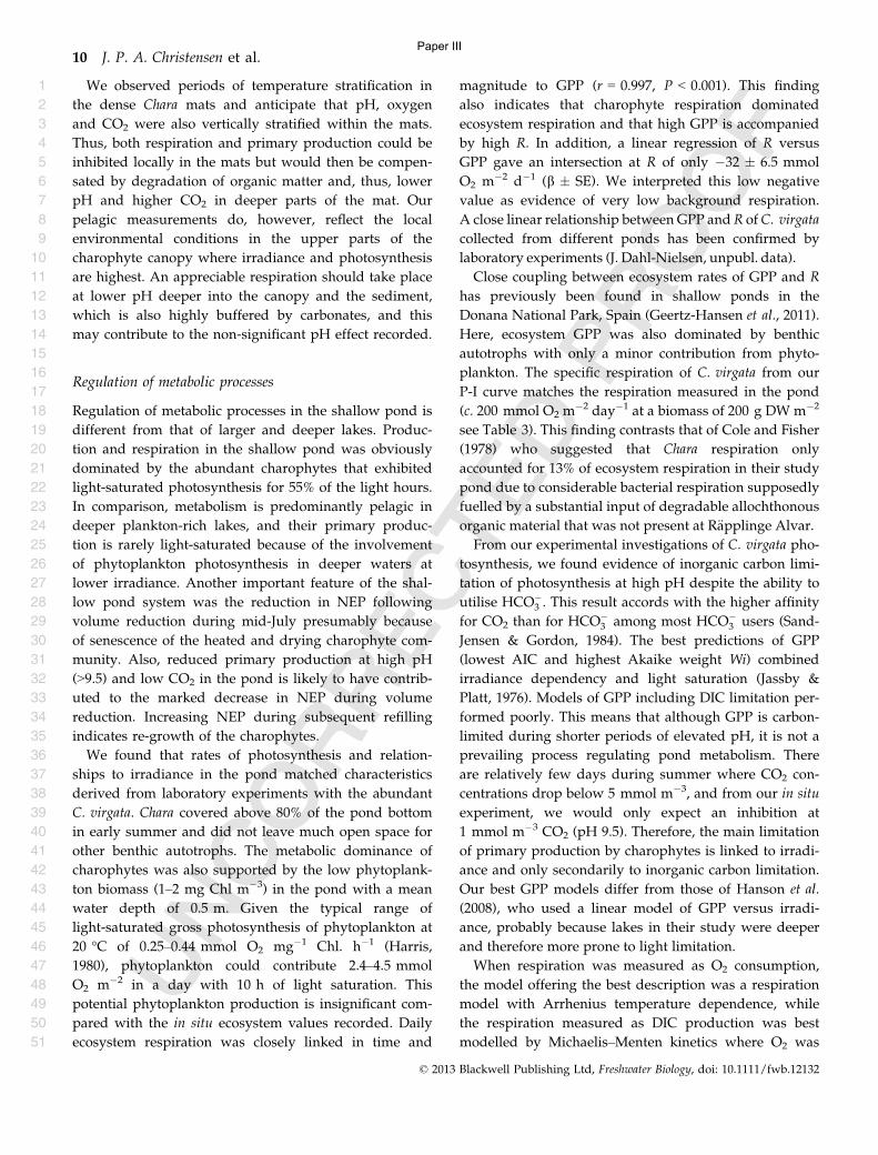
We observed periods of temperature stratification in

the dense Chara mats and anticipate that pH, oxygen

and CO2 were also vertically stratified within the mats.

Thus, both respiration and primary production could be

inhibited locally in the mats but would then be compen-

sated by degradation of organic matter and, thus, lower

pH and higher CO2 in deeper parts of the mat. Our

pelagic measurements do, however, reflect the local

environmental conditions in the upper parts of the

charophyte canopy where irradiance and photosynthesis

are highest. An appreciable respiration should take place

at lower pH deeper into the canopy and the sediment,

which is also highly buffered by carbonates, and this

may contribute to the non-significant pH effect recorded.

Regulation of metabolic processes

Regulation of metabolic processes in the shallow pond is

different from that of larger and deeper lakes. Produc-

tion and respiration in the shallow pond was obviously

dominated by the abundant charophytes that exhibited

light-saturated photosynthesis for 55% of the light hours.

In comparison, metabolism is predominantly pelagic in

deeper plankton-rich lakes, and their primary produc-

tion is rarely light-saturated because of the involvement

of phytoplankton photosynthesis in deeper waters at

lower irradiance. Another important feature of the shal-

low pond system was the reduction in NEP following

volume reduction during mid-July presumably because

of senescence of the heated and drying charophyte com-

munity. Also, reduced primary production at high pH

(>9.5) and low CO2 in the pond is likely to have contrib-

uted to the marked decrease in NEP during volume

reduction. Increasing NEP during subsequent refilling

indicates re-growth of the charophytes.

We found that rates of photosynthesis and relation-

ships to irradiance in the pond matched characteristics

derived from laboratory experiments with the abundant

C. virgata. Chara covered above 80% of the pond bottom

in early summer and did not leave much open space for

other benthic autotrophs. The metabolic dominance of

charophytes was also supported by the low phytoplank-

ton biomass (1–2 mg Chl m�3) in the pond with a mean

water depth of 0.5 m. Given the typical range of

light-saturated gross photosynthesis of phytoplankton at

20 °C of 0.25–0.44 mmol O2 mg�1 Chl. h�1 (Harris,

1980), phytoplankton could contribute 2.4–4.5 mmol

O2 m�2 in a day with 10 h of light saturation. This

potential phytoplankton production is insignificant com-

pared with the in situ ecosystem values recorded. Daily

ecosystem respiration was closely linked in time and

magnitude to GPP (r = 0.997, P < 0.001). This finding

also indicates that charophyte respiration dominated

ecosystem respiration and that high GPP is accompanied

by high R. In addition, a linear regression of R versus

GPP gave an intersection at R of only �32 � 6.5 mmol

O2 m�2 d�1 (b � SE). We interpreted this low negative

value as evidence of very low background respiration.

A close linear relationship between GPP and R of C. virgata

collected from different ponds has been confirmed by

laboratory experiments (J. Dahl-Nielsen, unpubl. data).

Close coupling between ecosystem rates of GPP and R

has previously been found in shallow ponds in the

Donana National Park, Spain (Geertz-Hansen et al., 2011).

Here, ecosystem GPP was also dominated by benthic

autotrophs with only a minor contribution from phyto-

plankton. The specific respiration of C. virgata from our

P-I curve matches the respiration measured in the pond

(c. 200 mmol O2 m�2 day�1 at a biomass of 200 g DW m�2

see Table 3). This finding contrasts that of Cole and Fisher

(1978) who suggested that Chara respiration only

accounted for 13% of ecosystem respiration in their study

pond due to considerable bacterial respiration supposedly

fuelled by a substantial input of degradable allochthonous

organic material that was not present at R€applinge Alvar.

From our experimental investigations of C. virgata pho-

tosynthesis, we found evidence of inorganic carbon limi-

tation of photosynthesis at high pH despite the ability to

utilise HCO�3 . This result accords with the higher affinity

for CO2 than for HCO�3 among most HCO�3 users (Sand-

Jensen & Gordon, 1984). The best predictions of GPP

(lowest AIC and highest Akaike weight Wi) combined

irradiance dependency and light saturation (Jassby &

Platt, 1976). Models of GPP including DIC limitation per-

formed poorly. This means that although GPP is carbon-

limited during shorter periods of elevated pH, it is not a

prevailing process regulating pond metabolism. There

are relatively few days during summer where CO2 con-

centrations drop below 5 mmol m�3, and from our in situ

experiment, we would only expect an inhibition at

1 mmol m�3 CO2 (pH 9.5). Therefore, the main limitation

of primary production by charophytes is linked to irradi-

ance and only secondarily to inorganic carbon limitation.

Our best GPP models differ from those of Hanson et al.

(2008), who used a linear model of GPP versus irradi-

ance, probably because lakes in their study were deeper

and therefore more prone to light limitation.

When respiration was measured as O2 consumption,

the model offering the best description was a respiration

model with Arrhenius temperature dependence, while

the respiration measured as DIC production was best

modelled by Michaelis–Menten kinetics where O2 was

© 2013 Blackwell Publishing Ltd, Freshwater Biology, doi: 10.1111/fwb.12132

10 J. P. A. Christensen et al.

1

2

3

4

5

6

7

8

9

10

11

12

13

14

15

16

17

18

19

20

21

22

23

24

25

26

27

28

29

30

31

32

33

34

35

36

37

38

39

40

41

42

43

44

45

46

47

48

49

50

51

Paper III

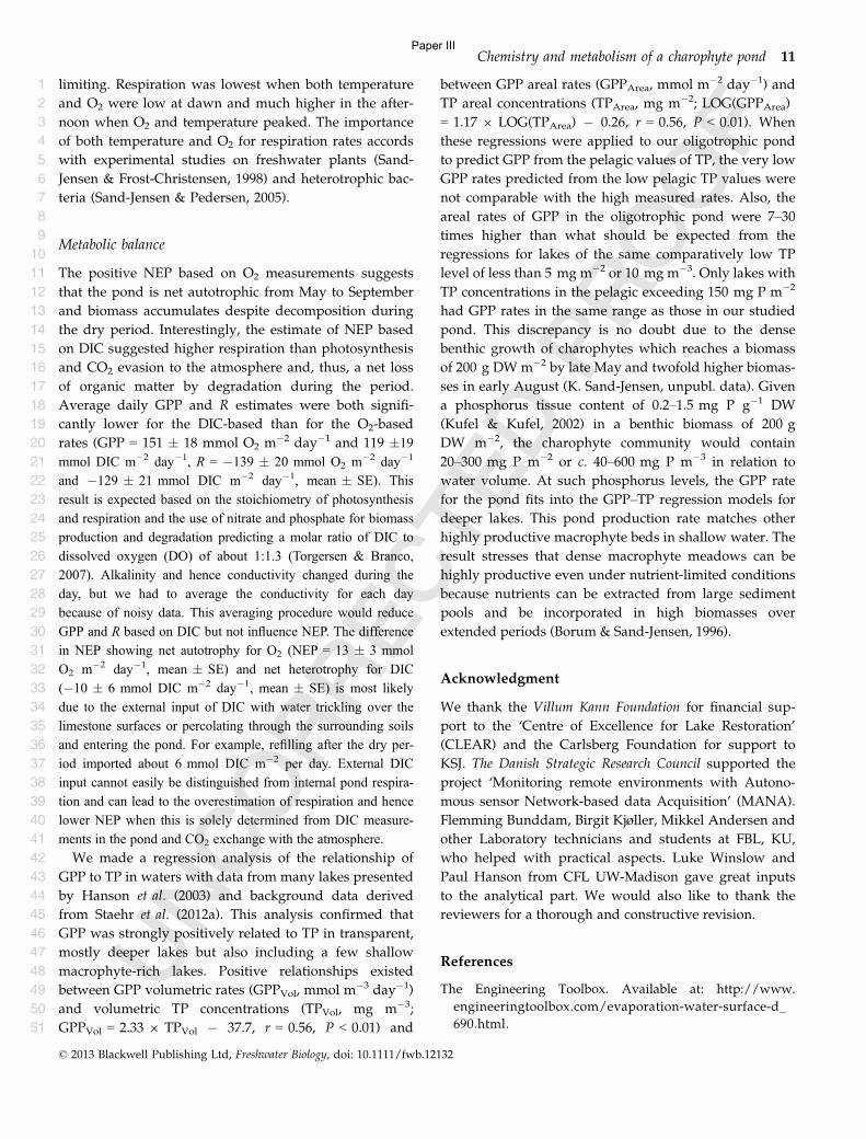
limiting. Respiration was lowest when both temperature

and O2 were low at dawn and much higher in the after-

noon when O2 and temperature peaked. The importance

of both temperature and O2 for respiration rates accords

with experimental studies on freshwater plants (Sand-

Jensen & Frost-Christensen, 1998) and heterotrophic bac-

teria (Sand-Jensen & Pedersen, 2005).

Metabolic balance

The positive NEP based on O2 measurements suggests

that the pond is net autotrophic from May to September

and biomass accumulates despite decomposition during

the dry period. Interestingly, the estimate of NEP based

on DIC suggested higher respiration than photosynthesis

and CO2 evasion to the atmosphere and, thus, a net loss

of organic matter by degradation during the period.

Average daily GPP and R estimates were both signifi-

cantly lower for the DIC-based than for the O2-based

rates (GPP = 151 � 18 mmol O2 m�2 day�1 and 119 �19mmol DIC m�2 day�1, R = �139 � 20 mmol O2 m�2 day�1

and �129 � 21 mmol DIC m�2 day�1, mean � SE). This

result is expected based on the stoichiometry of photosynthesis

and respiration and the use of nitrate and phosphate for biomass

production and degradation predicting a molar ratio of DIC to

dissolved oxygen (DO) of about 1:1.3 (Torgersen & Branco,

2007). Alkalinity and hence conductivity changed during the

day, but we had to average the conductivity for each day

because of noisy data. This averaging procedure would reduce

GPP and R based on DIC but not influence NEP. The difference

in NEP showing net autotrophy for O2 (NEP = 13 � 3 mmol

O2 m�2 day�1, mean � SE) and net heterotrophy for DIC

(�10 � 6 mmol DIC m�2 day�1, mean � SE) is most likely

due to the external input of DIC with water trickling over the

limestone surfaces or percolating through the surrounding soils

and entering the pond. For example, refilling after the dry per-

iod imported about 6 mmol DIC m�2 per day. External DIC

input cannot easily be distinguished from internal pond respira-

tion and can lead to the overestimation of respiration and hence

lower NEP when this is solely determined from DIC measure-

ments in the pond and CO2 exchange with the atmosphere.

We made a regression analysis of the relationship of

GPP to TP in waters with data from many lakes presented

by Hanson et al. (2003) and background data derived

from Staehr et al. (2012a). This analysis confirmed that

GPP was strongly positively related to TP in transparent,

mostly deeper lakes but also including a few shallow

macrophyte-rich lakes. Positive relationships existed

between GPP volumetric rates (GPPVol, mmol m�3 day�1)

and volumetric TP concentrations (TPVol, mg m�3;

GPPVol = 2.33 9 TPVol � 37.7, r = 0.56, P < 0.01) and

between GPP areal rates (GPPArea, mmol m�2 day�1) and

TP areal concentrations (TPArea, mg m�2; LOG(GPPArea)

= 1.17 9 LOG(TPArea) � 0.26, r = 0.56, P < 0.01). When

these regressions were applied to our oligotrophic pond

to predict GPP from the pelagic values of TP, the very low

GPP rates predicted from the low pelagic TP values were

not comparable with the high measured rates. Also, the

areal rates of GPP in the oligotrophic pond were 7–30

times higher than what should be expected from the

regressions for lakes of the same comparatively low TP

level of less than 5 mg m�2 or 10 mg m�3. Only lakes with

TP concentrations in the pelagic exceeding 150 mg P m�2

had GPP rates in the same range as those in our studied

pond. This discrepancy is no doubt due to the dense

benthic growth of charophytes which reaches a biomass

of 200 g DW m�2 by late May and twofold higher biomas-

ses in early August (K. Sand-Jensen, unpubl. data). Given

a phosphorus tissue content of 0.2–1.5 mg P g�1 DW

(Kufel & Kufel, 2002) in a benthic biomass of 200 g

DW m�2, the charophyte community would contain

20–300 mg P m�2 or c. 40–600 mg P m�3 in relation to

water volume. At such phosphorus levels, the GPP rate

for the pond fits into the GPP–TP regression models for

deeper lakes. This pond production rate matches other

highly productive macrophyte beds in shallow water. The

result stresses that dense macrophyte meadows can be

highly productive even under nutrient-limited conditions

because nutrients can be extracted from large sediment

pools and be incorporated in high biomasses over

extended periods (Borum & Sand-Jensen, 1996).

Acknowledgment

We thank the Villum Kann Foundation for financial sup-

port to the ‘Centre of Excellence for Lake Restoration’

(CLEAR) and the Carlsberg Foundation for support to

KSJ. The Danish Strategic Research Council supported the

project ‘Monitoring remote environments with Autono-

mous sensor Network-based data Acquisition’ (MANA).

Flemming Bunddam, Birgit Kjøller, Mikkel Andersen and

other Laboratory technicians and students at FBL, KU,

who helped with practical aspects. Luke Winslow and

Paul Hanson from CFL UW-Madison gave great inputs

to the analytical part. We would also like to thank the

reviewers for a thorough and constructive revision.

References

The Engineering Toolbox. Available at: http://www.

engineeringtoolbox.com/evaporation-water-surface-d_

690.html.

© 2013 Blackwell Publishing Ltd, Freshwater Biology, doi: 10.1111/fwb.12132

Chemistry and metabolism of a charophyte pond 11

1

2

3

4

5

6

7

8

9

10

11

12

13

14

15

16

17

18

19

20

21

22

23

24

25

26

27

28

29

30

31

32

33

34

35

36

37

38

39

40

41

42

43

44

45

46

47

48

49

50

51

Paper III

Arle J. (2002) Physical and chemical dynamics of temporary

ponds on a calcareous plateau in Thuringia, Germany.

Limnologica – Ecology and Management of Inland Waters, 32,

83–101.

Bade D.L. & Cole J.J. (2006) Impact of chemically enhanced

diffusion on dissolved inorganic carbon stable isotopes in

a fertilized lake. Journal of Geophysical Reserach, 111,

C01014.

Borum J. & Sand-Jensen K. (1996) Is total primary produc-

tion in shallow coastal marine waters stimulated by nitro-

gen loading? Oikos, 76, 406–410.

Boulton A.J. & Brock M.A. (1999) Australian Freshwater Ecol-

ogy: Processes and Management. Gleneagles Publishing,

Mount Osmond, SA.

Burnham K.P. & Anderson D.R. (2004) Multimodel infer-

ence – understanding AIC and BIC in model selection.

Sociological Methods & Research, 33, 261–304.

Cogley J.G. (1979) The albedo of water as a function of

latitude. Monthly Weather Review, 107, 775–781.

Cole J., Prairie Y., Caraco N., Mcdowell W., Tranvik L.,

Striegl R. et al. (2007) Plumbing the global carbon cycle:

integrating inland waters into the terrestrial carbon

budget. Ecosystems, 10, 172–185.

Cole J.J. & Caraco N.F. (1998) Atmospheric exchange of

carbon dioxide in a low-wind oligotrophic lake measured

by the addition of SF6. Limnology and Oceanography, 43,

647–656.

Downing J.A., Prairie Y.T., Cole J.J., Duarte C.M., Tranvik

L.J., Striegl R.G. et al. (2006) The global abundance and

size distribution of lakes, ponds, and impoundments.

Limnology and Oceanography, 51, 2388–2397.

Geertz-Hansen O., Montes C., Duarte C.M., Sand-Jensen K.,

Marba N. & Grillas P. (2011) Ecosystem metabolism in a

temporary Mediterranean marsh (Donana National Park,

SW Spain). Biogeosciences, 8, 963–971.

Hanson P.C., Bade D.L., Carpenter S.R. & Kratz T.K. (2003)

Lake metabolism: relationships with dissolved organic

carbon and phosphorus. Limnology and Oceanography, 48,

1112–1119.

Hanson P.C., Carpenter S.R., Kimura N., Wu C., Cornelius

S.P. & Kratz T.K. (2008) Evaluation of metabolism models

for free-water dissolved oxygen methods in lakes. Limnol-

ogy and Oceanography-Methods, 6, 454–465.

Harris G. (1980) The measurement of photosynthesis in nat-

ural populations of phytoplankton. In: Studies in Ecology

(Ed. ???? ), pp. 129–187. University of California

Press, Berkeley, CA.

Jahne B., Heinz G. & Dietrich W. (1987a) Measurement of

the diffusion-coefficients of sparingly soluble gases in

water. Journal of Geophysical Research-Oceans, 92, 10767–

10776.

Jahne B., Munnich K.O., Bosinger R., Dutzi A., Huber W. &

Libner P. (1987b) On the parameters influencing air-water

gas-exchange. Journal of Geophysical Research-Oceans, 92,

1937–1949.

Jassby A.D. & Platt T. (1976) Mathematical formulation of

relationship between photosynthesis and light for phyto-

planktion. Limnology and Oceanography, 21, 540–547.

Jorgensen S.E. & Bendoricchio G. (2001) Fundamentals of

Ecological Modelling, 3rd edn. Elsevier, Amsterdam.

Kufel L. & Kufel I. (2002) Chara beds acting as nutrient sinks

in shallow lakes—a review. Aquatic Botany, 72, 249–260.

Maberly S.C. & Madsen T.V. (2002) Freshwater angiosperm

carbon concentrating mechanisms: processes and pat-

terns. Functional Plant Biology, 29, 393–405.

Mackereth F.J.H., Heron J. & Talling J.F. (1978) Water Analy-

sis: Some Revised Methods for Limnologists. Freshwater

Biological Association, Ambleside, UK, pp. 1–120.

McConnaughey T. (1991) Calcification in Chara-corallina -

CO2 hydroxylation generates protons for bicarbonate

assimilation. Limnology and Oceanography, 36, 619–628.

Odum H.T. (1956) Primary production in flowing waters.

Limnology and Oceanography, 1, 102–117.

Penman H.L. (1948) Natural evaporation from open water,

bare soil and grass. Proceedings of the Royal Society of Lon-

don. Series A. Mathematical and Physical Sciences, 193,

120–145.

Pierson D.C., Pettersson K. & Istvanovics V. (1992) Tempo-

ral changes in biomass specific photosynthesis during the

summer: regulation by environmental factors and the

importance of phytoplankton succession. Hydrobiologia,

243–244, 119–135.

Rebsdorf A., Søndergaard ????. & Thyssen N.. (1988)

Overv�agningsprogram. Vand- og sedimentanalyser i ferskvand.

Særlige kemiske analyse- og beregningsmetoder Miljøstyrel-

sens Ferskvandslaboratorium.

Sand-Jensen K., Baastrup-Spohr L., Winkel A., Moller C.L.,

Borum J., Brodersen K.P. et al. (2010) Plant distribution

patterns and adaptations in a limestone quarry on Oland.

Svensk Botanisk Tidskrift, 104, 23–31.

Sand-Jensen K. & Frost-Christensen H. (1998) Photosynthe-

sis of amphibious and obligately submerged plants in

CO2-rich lowland streams. Oecologia, 117, 31–39.

Sand-Jensen K. & Gordon D.M. (1984) Differential ability of

marine and freshwater macrophytes to utilize HCO3�

and CO2. Marine Biology, 80, 247–253.

Sand-Jensen K. & Jespersen T.S. (2012) Tolerance of the

widespread cyanobacterium Nostoc commune to extreme

temperature variations (�269 to 105°C), pH and salt

stress. Oecologia, 169, 331–339.

Sand-Jensen K. & Pedersen N.L. (2005) Differences in

temperature, organic carbon and oxygen consumption

among lowland streams. Freshwater Biology, 50, 1927–1937.

Sand-Jensen K. & Staehr P.A. (2009) Net heterotrophy in

small Danish lakes: a widespread feature over gradients

in trophic status and land cover. Ecosystems, 12, 336–348.

Staehr P.A., Baastrup-Spohr L., Sand-Jensen K. & Stedmon C.

(2012a) Lake metabolism scales with lake morphometry

and catchment conditions. Aquatic Sciences-Research Across

Boundaries, 74, 155–169.

© 2013 Blackwell Publishing Ltd, Freshwater Biology, doi: 10.1111/fwb.12132

12 J. P. A. Christensen et al.

1

2

3

4

5

6

7

8

9

10

11

12

13

14

15

16

17

18

19

20

21

22

23

24

25

26

27

28

29

30

31

32

33

34

35

36

37

38

39

40

41

42

43

44

45

46

47

48

49

50

51

Paper III

Staehr P.A. & Sand-Jensen K. (2006) Seasonal changes in

temperature and nutrient control of photosynthesis, respi-

ration and growth of natural phytoplankton communities.

Freshwater Biology, 51, 249–262.

Staehr P.A., Testa J.M., Kemp W.M., Cole J.J., Sand-Jensen

K. & Smith S.V. (2012b) The metabolism of aquatic

ecosystems: history, applications, and future challenges.

Aquatic Sciences-Research Across Boundaries, 74, 15–29.

Tank S.E., Lesack L.F.W. & Mcqueen D.J. (2009) Elevated

pH regulates bacterial carbon cycling in lakes with high

photosynthetic activity. Ecology, 90, 1910–1922.

Torgersen T. & Branco B. (2007) Carbon and oxygen dynamics

of shallow aquatic systems: process vectors and bacterial

productivity. Journal of Geophysical Research, 112, G03016.

Tranvik L.J., Downing J.A., Cotner J.B., Loiselle S.A., Striegl

R.G., Ballatore T.J. et al. (2009) Lakes and reservoirs as

regulators of carbon cycling and climate. Limnology and

Oceanography, 54, 2298–2314.

Van T.K., Haller W.T. & Bowes G. (1976) Comparison of

photosynthetic characteristics of 3 submersed aquatic

plants. Plant Physiology, 58, 761–768.

Vermaat J.E. & Sand-Jensen K. (1987) Survival, metabolism

and growth of Ulva lactuca under winter conditions: a

laboratory study of bottlenecks in the life cycle. Marine

Biology, 95, 55–61.

Wanninkhof R. (1992) Relationship between wind-speed

and gas-exchange over the ocean. Journal of Geophysical

Research-Oceans, 97, 7373–7382.

Williams P., Whitfield M., Biggs J., Bray S., Fox G., Nicolet

P. et al. (2004) Comparative biodiversity of rivers,

streams, ditches and ponds in an agricultural landscape

in Southern England. Biological Conservation, 115, 329–341.

Williams W.D. (1985) Biotic adaptations in temporary lentic

waters, with special reference to those in semi-arid and

arid regions. Hydrobiologia, 125, 85–110.

Xu C.Y. & Singh V. (2002) Cross comparison of empirical

equations for calculating potential evapotranspiration

with data from Switzerland. Water Resources Management,

16, 197–219.

(Manuscript accepted 21 February 2013)

© 2013 Blackwell Publishing Ltd, Freshwater Biology, doi: 10.1111/fwb.12132

Chemistry and metabolism of a charophyte pond 13

1

2

3

4

5

6

7

8

9

10

11

12

13

14

15

16

17

18

19

20

21

22

23

24

25

26

27

28

29

30

31

32

33

34

35

36

37

38

39

40

41

42

43

44

45

46

47

48

49

50

51

Paper III

82

Paper IV

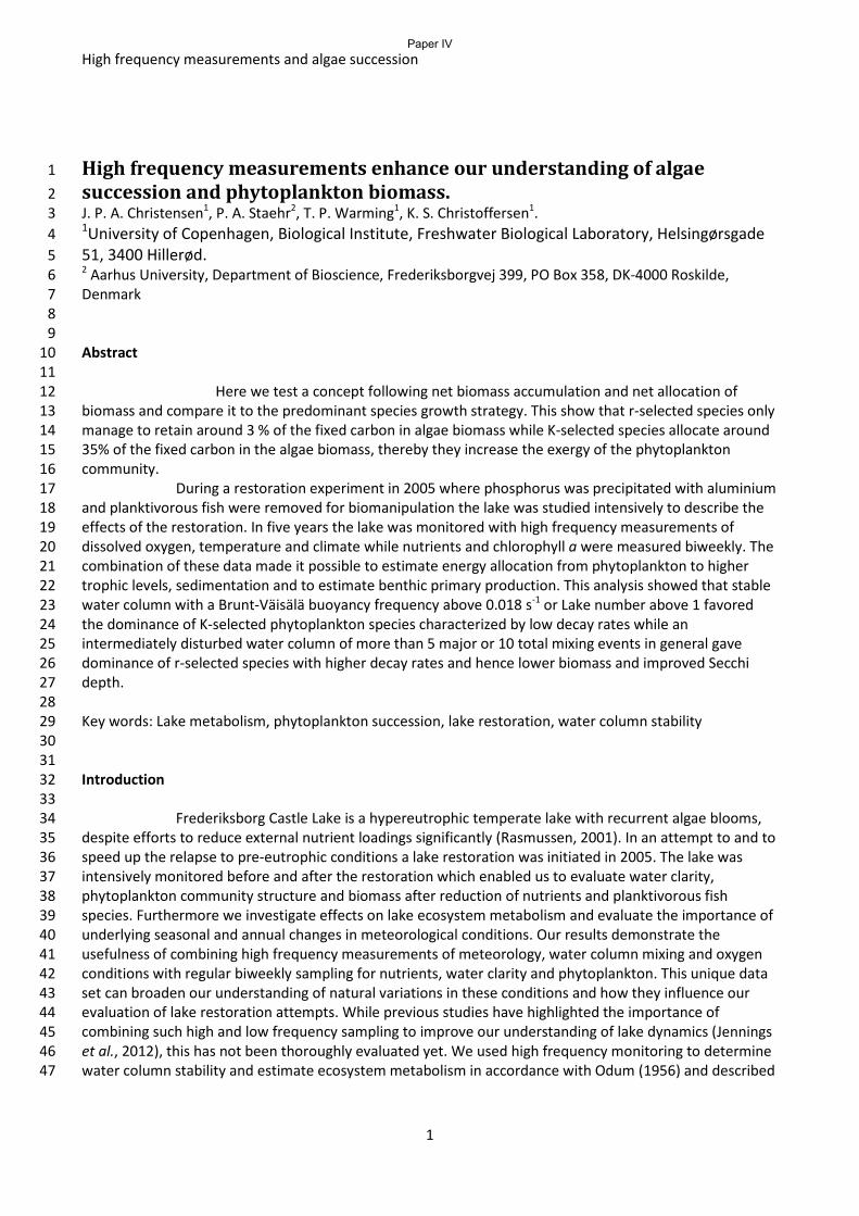
High frequency measurements and algae succession

1

High frequency measurements enhance our understanding of algae 1 succession and phytoplankton biomass. 2 J. P. A. Christensen1, P. A. Staehr2, T. P. Warming1, K. S. Christoffersen1. 3 1University of Copenhagen, Biological Institute, Freshwater Biological Laboratory, Helsingørsgade 4 51, 3400 Hillerød. 5 2 Aarhus University, Department of Bioscience, Frederiksborgvej 399, PO Box 358, DK-4000 Roskilde, 6 Denmark 7 8 9 Abstract 10 11

Here we test a concept following net biomass accumulation and net allocation of 12 biomass and compare it to the predominant species growth strategy. This show that r-selected species only 13 manage to retain around 3 % of the fixed carbon in algae biomass while K-selected species allocate around 14 35% of the fixed carbon in the algae biomass, thereby they increase the exergy of the phytoplankton 15 community. 16

During a restoration experiment in 2005 where phosphorus was precipitated with aluminium 17 and planktivorous fish were removed for biomanipulation the lake was studied intensively to describe the 18 effects of the restoration. In five years the lake was monitored with high frequency measurements of 19 dissolved oxygen, temperature and climate while nutrients and chlorophyll a were measured biweekly. The 20 combination of these data made it possible to estimate energy allocation from phytoplankton to higher 21 trophic levels, sedimentation and to estimate benthic primary production. This analysis showed that stable 22 water column with a Brunt-Väisälä buoyancy frequency above 0.018 s-1 or Lake number above 1 favored 23 the dominance of K-selected phytoplankton species characterized by low decay rates while an 24 intermediately disturbed water column of more than 5 major or 10 total mixing events in general gave 25 dominance of r-selected species with higher decay rates and hence lower biomass and improved Secchi 26 depth. 27 28 Key words: Lake metabolism, phytoplankton succession, lake restoration, water column stability 29 30 31 Introduction 32 33

Frederiksborg Castle Lake is a hypereutrophic temperate lake with recurrent algae blooms, 34 despite efforts to reduce external nutrient loadings significantly (Rasmussen, 2001). In an attempt to and to 35 speed up the relapse to pre-eutrophic conditions a lake restoration was initiated in 2005. The lake was 36 intensively monitored before and after the restoration which enabled us to evaluate water clarity, 37 phytoplankton community structure and biomass after reduction of nutrients and planktivorous fish 38 species. Furthermore we investigate effects on lake ecosystem metabolism and evaluate the importance of 39 underlying seasonal and annual changes in meteorological conditions. Our results demonstrate the 40 usefulness of combining high frequency measurements of meteorology, water column mixing and oxygen 41 conditions with regular biweekly sampling for nutrients, water clarity and phytoplankton. This unique data 42 set can broaden our understanding of natural variations in these conditions and how they influence our 43 evaluation of lake restoration attempts. While previous studies have highlighted the importance of 44 combining such high and low frequency sampling to improve our understanding of lake dynamics (Jennings 45 et al., 2012), this has not been thoroughly evaluated yet. We used high frequency monitoring to determine 46 water column stability and estimate ecosystem metabolism in accordance with Odum (1956) and described 47

Paper IV

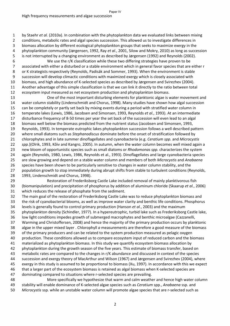
High frequency measurements and algae succession

2

by Staehr et al. (2010a). In combination with the phytoplankton data we evaluated links between mixing 1 conditions, metabolic rates and algal species succession. This allowed us to investigate differences in 2 biomass allocation by different ecological phytoplankton groups that seeks to maximize exergy in the 3 phytoplankton community (Jørgensen, 1992, Ray et al., 2001, Silow and Mokry, 2010) as long as succession 4 is not interrupted by a changing environment as described by Jørgensen (1992) and Reynolds (2002). 5

We use the r/K classification while these two differing strategies have proven to be 6 associated with either a disturbed or a stable environment which in general favor species that are either r 7 or K strategists respectively (Reynolds, Padisák and Sommer, 1993). When the environment is stable 8 succession will develop climactic conditions with maximized exergy which is closely associated with 9 biomass, and high abundance of K-selected species as described by Jørgensen and Svirezhev (2004). 10 Another advantage of this simple classification is that we can link it directly to the ratio between total 11 ecosystem input measured as net ecosystem production and phytoplankton biomass. 12

One of the most important disturbing elements for planktonic algae is water movement and 13 water column stability (Lindenschmidt and Chorus, 1998). Many studies have shown how algal succession 14 can be completely or partly set back by mixing events during a period with stratified water column in 15 temperate lakes (Lewis, 1986, Jacobsen and Simonsen, 1993, Reynolds et al., 1993). At an intermediate 16 disturbance frequency of 8-50 times per year the set back of the succession will even lead to an algal 17 biomass well below the biomass predicted from the nutrient status (Jacobsen and Simonsen, 1993, 18 Reynolds, 1993). In temperate eutrophic lakes phytoplankton succession follows a well described pattern 19 where small diatoms such as Stephanodiscus dominate before the onset of stratification followed by 20 chlorophytes and in late summer dinoflagellates and cyanobacteria (e.g. Ceratium spp. and Microcystis 21 spp.)(Olrik, 1993, Kõiv and Kangro, 2005). In autumn, when the water column becomes well mixed again a 22 new bloom of opportunistic species such as small diatoms or Rhodomonas spp. characterizes the system 23 again (Reynolds, 1980, Lewis, 1986, Reynolds et al., 1993). Dinoflagellates and large cyanobacteria species 24 are slow growing and depend on a stable water column and members of both Microcystis and Anabaena 25 species have been shown to be particularly sensitive to changes in water column stability, and the 26 population growth to stop immediately during abrupt shifts from stable to turbulent conditions (Reynolds, 27 1993, Lindenschmidt and Chorus, 1998). 28

Restoration of Frederiksborg Castle Lake included removal of mainly planktivorous fish 29 (biomanipulation) and precipitation of phosphorus by addition of aluminum chloride (Skaarup et al., 2006) 30 which reduces the release of phosphate from the sediment. 31 The main goal of the restoration of Frederiksborg Castle Lake was to reduce phytoplankton biomass and 32 the risk of cyanobacterial blooms, as well as improve water clarity and benthic life conditions. Phosphorus 33 levels is generally found to control primary production (Hanson et al., 2003) and the maximum 34 phytoplankton density (Schindler, 1977). In a hypereutrophic, turbid lake such as Frederiksborg Castle lake, 35 low light conditions impedes growth of submerged macrophytes and benthic microalgae (Cazzanelli, 36 Warming and Christoffersen, 2008) and hence the majority of the primary production occurs by planktonic 37 algae in the upper mixed layer . Chlorophyll a measurements are therefore a good measure of the biomass 38 of the primary producers and can be related to the system production measured as pelagic oxygen 39 production. These conditions allowed us to compare ecosystem input of reduced carbon and the biomass 40 materialized as phytoplankton biomass. In this study we quantify ecosystem biomass allocation by 41 phytoplankton during the growth season of the five years. This estimate of biomass transfer, based on 42 metabolic rates are compared to the changes in r/K abundance and discussed in context of the species 43 succession and exergy theory of MacArthur and Wilson (1967) and Jørgensen and Svirezhev (2004), where 44 exergy in this study is assumed to be proportional to biomass (Xu, 1997). In accordance with this we expect 45 that a larger part of the ecosystem biomass is retained as algal biomass when K-selected species are 46 dominating compared to situations where r-selected species are prevailing. 47

More specifically we hypothesize that warm and calm weather and hence high water column 48 stability will enable dominance of K-selected algae species such as Ceratium spp., Anabaena ssp. and 49 Microcystis ssp. while an unstable water column will promote algae species that are r-selected such as 50

Paper IV

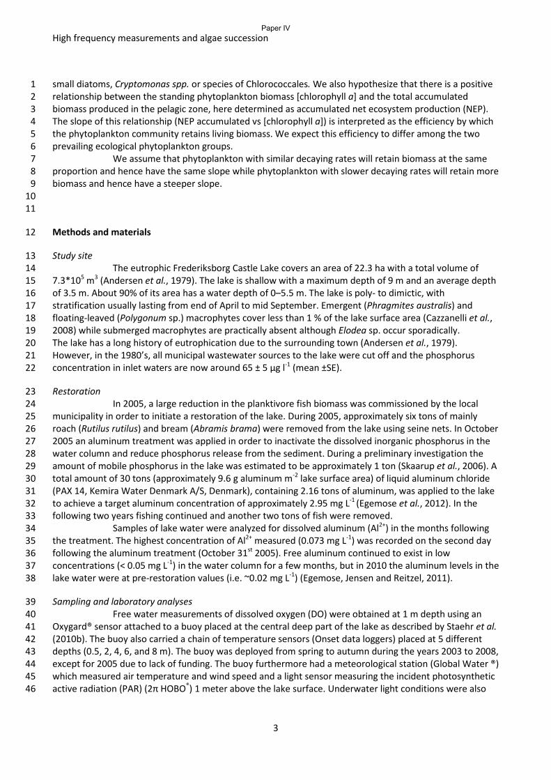
High frequency measurements and algae succession

3

small diatoms, Cryptomonas spp. or species of Chlorococcales. We also hypothesize that there is a positive 1 relationship between the standing phytoplankton biomass [chlorophyll a] and the total accumulated 2 biomass produced in the pelagic zone, here determined as accumulated net ecosystem production (NEP). 3 The slope of this relationship (NEP accumulated vs [chlorophyll a]) is interpreted as the efficiency by which 4 the phytoplankton community retains living biomass. We expect this efficiency to differ among the two 5 prevailing ecological phytoplankton groups. 6

We assume that phytoplankton with similar decaying rates will retain biomass at the same 7 proportion and hence have the same slope while phytoplankton with slower decaying rates will retain more 8 biomass and hence have a steeper slope. 9 10 11

Methods and materials 12

Study site 13 The eutrophic Frederiksborg Castle Lake covers an area of 22.3 ha with a total volume of 14

7.3*105 m3 (Andersen et al., 1979). The lake is shallow with a maximum depth of 9 m and an average depth 15 of 3.5 m. About 90% of its area has a water depth of 0–5.5 m. The lake is poly- to dimictic, with 16 stratification usually lasting from end of April to mid September. Emergent (Phragmites australis) and 17 floating-leaved (Polygonum sp.) macrophytes cover less than 1 % of the lake surface area (Cazzanelli et al., 18 2008) while submerged macrophytes are practically absent although Elodea sp. occur sporadically. 19 The lake has a long history of eutrophication due to the surrounding town (Andersen et al., 1979). 20 However, in the 1980’s, all municipal wastewater sources to the lake were cut off and the phosphorus 21 concentration in inlet waters are now around 65 ± 5 µg l-1 (mean ±SE). 22

Restoration 23 In 2005, a large reduction in the planktivore fish biomass was commissioned by the local 24

municipality in order to initiate a restoration of the lake. During 2005, approximately six tons of mainly 25 roach (Rutilus rutilus) and bream (Abramis brama) were removed from the lake using seine nets. In October 26 2005 an aluminum treatment was applied in order to inactivate the dissolved inorganic phosphorus in the 27 water column and reduce phosphorus release from the sediment. During a preliminary investigation the 28 amount of mobile phosphorus in the lake was estimated to be approximately 1 ton (Skaarup et al., 2006). A 29 total amount of 30 tons (approximately 9.6 g aluminum m-2 lake surface area) of liquid aluminum chloride 30 (PAX 14, Kemira Water Denmark A/S, Denmark), containing 2.16 tons of aluminum, was applied to the lake 31 to achieve a target aluminum concentration of approximately 2.95 mg L-1 (Egemose et al., 2012). In the 32 following two years fishing continued and another two tons of fish were removed. 33

Samples of lake water were analyzed for dissolved aluminum (Al2+) in the months following 34 the treatment. The highest concentration of Al2+ measured (0.073 mg L-1) was recorded on the second day 35 following the aluminum treatment (October 31st 2005). Free aluminum continued to exist in low 36 concentrations (< 0.05 mg L-1) in the water column for a few months, but in 2010 the aluminum levels in the 37 lake water were at pre-restoration values (i.e. ~0.02 mg L-1) (Egemose, Jensen and Reitzel, 2011). 38

Sampling and laboratory analyses 39 Free water measurements of dissolved oxygen (DO) were obtained at 1 m depth using an 40

Oxygard® sensor attached to a buoy placed at the central deep part of the lake as described by Staehr et al. 41 (2010b). The buoy also carried a chain of temperature sensors (Onset data loggers) placed at 5 different 42 depths (0.5, 2, 4, 6, and 8 m). The buoy was deployed from spring to autumn during the years 2003 to 2008, 43 except for 2005 due to lack of funding. The buoy furthermore had a meteorological station (Global Water ®) 44 which measured air temperature and wind speed and a light sensor measuring the incident photosynthetic 45 active radiation (PAR) (2π HOBO®) 1 meter above the lake surface. Underwater light conditions were also 46

Paper IV

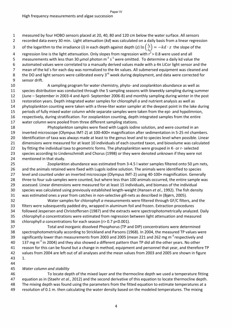
High frequency measurements and algae succession

4

measured by four HOBO sensors placed at 20, 40, 80 and 120 cm below the water surface. All sensors 1 recorded data every 30 min. Light attenuation (kd) was calculated on a daily basis from a linear regression 2 of the logarithm to the irradiance (i) in each depth against depth (z) ln � 𝐼𝑧

𝐼0� = −𝑘𝑑 ∙ 𝑧 the slope of the 3

regression line is the light attenuation. Only slopes from regression with r2 > 0.8 were used and all 4 measurements with less than 30 µmol photon m-2 s-1 were omitted. To determine a daily kd value the 5 automated values were correlated to a manually derived values made with a 4π LiCor light sensor and the 6 mean of the kd´s for each day was normalized to the 4π values. All submersed equipment was cleaned and 7 the DO and light sensors were calibrated every 3rd week during deployment, and data were corrected for 8 sensor drift. 9

A sampling program for water chemistry, phyto- and zooplankton abundance as well as 10 species distribution was conducted through the 5 sampling seasons with biweekly sampling during summer 11 (June – September in 2003-4 and April- September 2006-8) and monthly sampling during winter in the post 12 restoration years. Depth integrated water samples for chlorophyll a and nutrient analysis as well as 13 phytoplankton counting were taken with a three-liter water sampler at the deepest point in the lake during 14 periods of fully mixed water column while separate samples were taken from the epi- and hypolimnion, 15 respectively, during stratification. For zooplankton counting, depth integrated samples from the entire 16 water column were pooled from three different sampling stations. 17

Phytoplankton samples were fixed with Lugols iodine solution, and were counted in an 18 inverted microscope (Olympus IMT-2) at 100-400× magnification after sedimentation in 5-25 ml chambers. 19 Identification of taxa was always made at least to the genus level and to species level when possible. Linear 20 dimensions were measured for at least 10 individuals of each counted taxon, and biovolume was calculated 21 by fitting the individual taxa to geometric forms. The phytoplankton were grouped in K- or r- selected 22 species according to Lindenschmidt and Chorus (1998) or they were denoted unknown if they were not 23 mentioned in that study. 24

Zooplankton abundance was estimated from 3-4.5 l water samples filtered onto 50 μm nets, 25 and the animals retained were fixed with Lugols iodine solution. The animals were identified to species 26 level and counted under an inverted microscope (Olympus IMT-2) using 40-100× magnification. Generally 27 three to four sub-samples were counted, but where less than 100 animals occurred, the entire sample was 28 assessed. Linear dimensions were measured for at least 15 individuals, and biomass of the individual 29 species was calculated using previously established length-weight (Hansen et al., 1992). The fish density 30 was estimated ones a year from catches in non-selective gill-nets as described in (Bjørn, 2005). 31 Water samples for chlorophyll a measurements were filtered through GF/C filters, and the 32 filters were subsequently padded dry, wrapped in aluminum foil and frozen. Extraction procedures 33 followed Jespersen and Christoffersen (1987) and the extracts were spectrophotometrically analyzed. Daily 34 chlorophyll a concentrations were estimated from regression between light attenuation and measured 35 chlorophyll a concentrations for each season (r> 0.7 p<0.001). 36

Total and inorganic dissolved Phosphorus (TP and DIP) concentrations were determined 37 spectrophotometrically according to Strickland and Parsons (1968). In 2004, the measured TP values were 38 significantly lower than measurements from 2003 and 2005 (mean 221 and 262 mg m-3 respectively and 39 137 mg m-3 in 2004) and they also showed a different pattern than TP did all the other years. No other 40 reason for this can be found but a change in method, equipment and personnel that year, and therefore TP 41 values from 2004 are left out of all analyses and the mean values from 2003 and 2005 are shown in figure 42 1. 43 44 Water column and stability 45 To locate depth of the mixed layer and the thermocline depth we used a temperature fitting 46 equation as in (Staehr et al., 2012) and the second derivative of this equation to locate thermocline depth. 47 The mixing depth was found using the parameters from the fitted equation to estimate temperatures at a 48 resolution of 0.1 m. then calculating the water density based on the modeled temperatures. The mixing 49

Paper IV

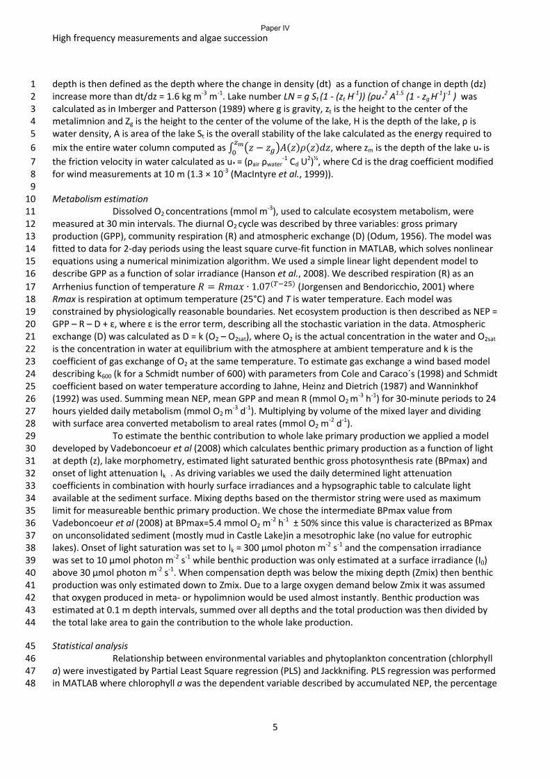
High frequency measurements and algae succession

5

depth is then defined as the depth where the change in density (dt) as a function of change in depth (dz) 1 increase more than dt/dz = 1.6 kg m-3 m-1. Lake number LN = g St (1 - (zt H-1)) (ρu*

2 A1.5 (1 - zg H-1)-1 ) was 2 calculated as in Imberger and Patterson (1989) where g is gravity, zt is the height to the center of the 3 metalimnion and Zg is the height to the center of the volume of the lake, H is the depth of the lake, ρ is 4 water density, A is area of the lake St is the overall stability of the lake calculated as the energy required to 5 mix the entire water column computed as ∫ �𝑧 − 𝑧𝑔�𝐴(𝑧)𝜌(𝑧)𝑑𝑧𝑧𝑚

0 , where zm is the depth of the lake u* is 6 the friction velocity in water calculated as u* = (ρair ρwater

-1 Cd U2)½, where Cd is the drag coefficient modified 7 for wind measurements at 10 m (1.3 × 10-3 (MacIntyre et al., 1999)). 8 9 Metabolism estimation 10

Dissolved O2 concentrations (mmol m-3), used to calculate ecosystem metabolism, were 11 measured at 30 min intervals. The diurnal O2 cycle was described by three variables: gross primary 12 production (GPP), community respiration (R) and atmospheric exchange (D) (Odum, 1956). The model was 13 fitted to data for 2-day periods using the least square curve-fit function in MATLAB, which solves nonlinear 14 equations using a numerical minimization algorithm. We used a simple linear light dependent model to 15 describe GPP as a function of solar irradiance (Hanson et al., 2008). We described respiration (R) as an 16 Arrhenius function of temperature 𝑅 = 𝑅𝑚𝑎𝑥 ∙ 1.07(𝑇−25) (Jorgensen and Bendoricchio, 2001) where 17 Rmax is respiration at optimum temperature (25°C) and T is water temperature. Each model was 18 constrained by physiologically reasonable boundaries. Net ecosystem production is then described as NEP = 19 GPP – R – D + ɛ, where ε is the error term, describing all the stochastic variation in the data. Atmospheric 20 exchange (D) was calculated as D = k (O2 – O2sat), where O2 is the actual concentration in the water and O2sat 21 is the concentration in water at equilibrium with the atmosphere at ambient temperature and k is the 22 coefficient of gas exchange of O2 at the same temperature. To estimate gas exchange a wind based model 23 describing k600 (k for a Schmidt number of 600) with parameters from Cole and Caraco´s (1998) and Schmidt 24 coefficient based on water temperature according to Jahne, Heinz and Dietrich (1987) and Wanninkhof 25 (1992) was used. Summing mean NEP, mean GPP and mean R (mmol O2 m-3 h-1) for 30-minute periods to 24 26 hours yielded daily metabolism (mmol O2 m-3 d-1). Multiplying by volume of the mixed layer and dividing 27 with surface area converted metabolism to areal rates (mmol O2 m-2 d-1). 28

To estimate the benthic contribution to whole lake primary production we applied a model 29 developed by Vadeboncoeur et al (2008) which calculates benthic primary production as a function of light 30 at depth (z), lake morphometry, estimated light saturated benthic gross photosynthesis rate (BPmax) and 31 onset of light attenuation Ik . As driving variables we used the daily determined light attenuation 32 coefficients in combination with hourly surface irradiances and a hypsographic table to calculate light 33 available at the sediment surface. Mixing depths based on the thermistor string were used as maximum 34 limit for measureable benthic primary production. We chose the intermediate BPmax value from 35 Vadeboncoeur et al (2008) at BPmax=5.4 mmol O2 m-2 h-1 ± 50% since this value is characterized as BPmax 36 on unconsolidated sediment (mostly mud in Castle Lake)in a mesotrophic lake (no value for eutrophic 37 lakes). Onset of light saturation was set to Ik = 300 µmol photon m-2 s-1 and the compensation irradiance 38 was set to 10 µmol photon m-2 s-1 while benthic production was only estimated at a surface irradiance (I0) 39 above 30 µmol photon m-2 s-1. When compensation depth was below the mixing depth (Zmix) then benthic 40 production was only estimated down to Zmix. Due to a large oxygen demand below Zmix it was assumed 41 that oxygen produced in meta- or hypolimnion would be used almost instantly. Benthic production was 42 estimated at 0.1 m depth intervals, summed over all depths and the total production was then divided by 43 the total lake area to gain the contribution to the whole lake production. 44

Statistical analysis 45 Relationship between environmental variables and phytoplankton concentration (chlorphyll 46

a) were investigated by Partial Least Square regression (PLS) and Jackknifing. PLS regression was performed 47 in MATLAB where chlorophyll a was the dependent variable described by accumulated NEP, the percentage 48

Paper IV

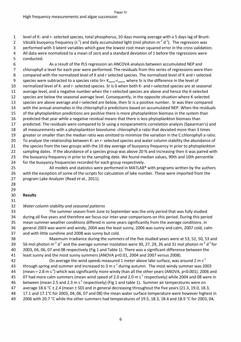
High frequency measurements and algae succession

6

level of K- and r- selected species, total phosphorus, 10 days moving average with a 5 days lag of Brunt-1 Väisälä buoyancy frequency (s-1) and daily accumulated light (mol photon m-2 d-1). The regression was 2 performed with 3 latent variables which gave the lowest root mean squared error in the cross validation. 3 All data were normalized to a mean of zero and a standard deviation of 1 before the regressions were 4 conducted. 5

As a result of the PLS regression an ANCOVA analysis between accumulated NEP and 6 chlorophyll a level for each year were performed. The residuals from this series of regressions were then 7 compared with the normalized level of K and r selected species. The normalized level of K and r selected 8 species were subtracted to a species ratio Sr= Knorm-rnorm, where Sr is the difference in the level of 9 normalized level of K- and r- selected species. Sr is 0 when both K- and r-selected species are at seasonal 10 average level, and a negative number when the r-selected species are above and hence the K-selected 11 species are below the seasonal average level. Consequently, in the opposite situation where K-selected 12 species are above average and r-selected are below, then Sr is a positive number. Sr was then compared 13 with the annual anomalies in the chlorophyll a predictions based on accumulated NEP. When the residuals 14 of the phytoplankton predictions are positive there is more phytoplankton biomass in the system than 15 predicted that year while a negative residual means that there is less phytoplankton biomass than 16 predicted. The residuals were compared to Sr using a nonparametric correlation analysis (Spearman’s) and 17 all measurements with a phytoplankton biovolume: chlorophyll a ratio that deviated more than 3 times 18 greater or smaller than the median ratio was omitted to minimize the variation in the C:chlorophyll a ratio. 19 To analyze the relationship between K- an r- selected species and water column stability the abundance of 20 the species from the two groups with the 10 day average of buoyancy frequency in prior to phytoplankton 21 sampling dates. If the abundance of a species group was above 20 % and increasing then it was paired with 22 the buoyancy frequency in prior to the sampling date. We found median values, 90th and 10th percentile 23 for the buoyancy frequencies recorded for each group respectively. 24 All models and statistics were performed in MATLAB® with programs written by the authors 25 with the exception of some of the scripts for calculation of lake number. These were imported from the 26 program Lake Analyzer (Read et al., 2011). 27 28 29 Results 30 31 Water column stability and seasonal patterns 32

The summer season from June to September was the only period that was fully studied 33 during all five years and therefore we focus our inter-year comparisons on this period. During this period 34 mean summer weather conditions differed in some years significantly from the average conditions. In 35 general 2003 was warm and windy, 2004 was the least sunny, 2006 was sunny and calm, 2007 cold, calm 36 and with little sunshine and 2008 was sunny but cold. 37

Maximum irradiance during the summers of the five studied years were at 53, 52, 50, 53 and 38 56 mol photon m-2 d-1 and the average summer insolation were 30, 27, 29, 26 and 31 mol photon m-2 d-1 for 39 2003, 04, 06, 07 and 08 respectively (Fig 1 and Table 1). There was a significant difference between the 40 least sunny and the most sunny summers (ANOVA p<0.01, 2004 and 2007 versus 2008). 41

On average the wind speeds measured 1 meter above lake surface, was around 2 m s-1 42 through spring and summer and increased to 3 m s-1 during autumn. The most windy summer was 2003 43 (mean = 2.8 m s-1) which was significantly more windy than all the other years (ANOVA, p<0.001). 2006 and 44 07 had more calm summers (mean wind speed of 2.0 and 2.0 m s-1 respectively) while 2004 and 08 were in 45 between (mean 2.5 and 2.3 m s-1 respectively) (Fig 1 and table 1). Summer air temperatures were on 46 average 18.6 °C ± 2.4 (mean ± SD) and in general decreasing throughout the five years (21.3, 19.0, 18.3, 47 17.1 and 17.1°C for 2003, 04, 06, 07 and 08) the mean water surface temperature were however highest in 48 2006 with 20.7 °C while the other summers had temperatures of 19.5, 18.3, 18.4 and 18.9 °C for 2003, 04, 49

Paper IV

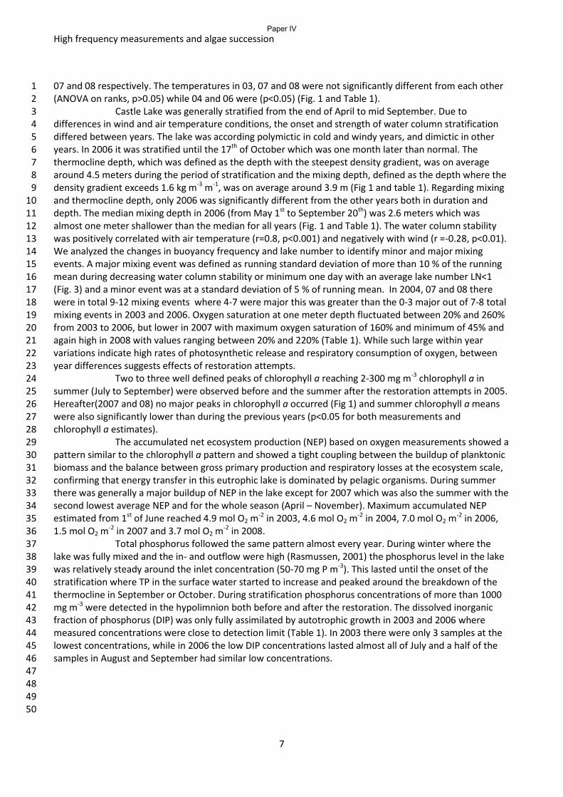
High frequency measurements and algae succession

7

07 and 08 respectively. The temperatures in 03, 07 and 08 were not significantly different from each other 1 (ANOVA on ranks, p>0.05) while 04 and 06 were (p<0.05) (Fig. 1 and Table 1). 2

Castle Lake was generally stratified from the end of April to mid September. Due to 3 differences in wind and air temperature conditions, the onset and strength of water column stratification 4 differed between years. The lake was according polymictic in cold and windy years, and dimictic in other 5 years. In 2006 it was stratified until the 17th of October which was one month later than normal. The 6 thermocline depth, which was defined as the depth with the steepest density gradient, was on average 7 around 4.5 meters during the period of stratification and the mixing depth, defined as the depth where the 8 density gradient exceeds 1.6 kg m-3 m-1, was on average around 3.9 m (Fig 1 and table 1). Regarding mixing 9 and thermocline depth, only 2006 was significantly different from the other years both in duration and 10 depth. The median mixing depth in 2006 (from May 1st to September 20th) was 2.6 meters which was 11 almost one meter shallower than the median for all years (Fig. 1 and Table 1). The water column stability 12 was positively correlated with air temperature (r=0.8, p<0.001) and negatively with wind (r =-0.28, p<0.01). 13 We analyzed the changes in buoyancy frequency and lake number to identify minor and major mixing 14 events. A major mixing event was defined as running standard deviation of more than 10 % of the running 15 mean during decreasing water column stability or minimum one day with an average lake number LN<1 16 (Fig. 3) and a minor event was at a standard deviation of 5 % of running mean. In 2004, 07 and 08 there 17 were in total 9-12 mixing events where 4-7 were major this was greater than the 0-3 major out of 7-8 total 18 mixing events in 2003 and 2006. Oxygen saturation at one meter depth fluctuated between 20% and 260% 19 from 2003 to 2006, but lower in 2007 with maximum oxygen saturation of 160% and minimum of 45% and 20 again high in 2008 with values ranging between 20% and 220% (Table 1). While such large within year 21 variations indicate high rates of photosynthetic release and respiratory consumption of oxygen, between 22 year differences suggests effects of restoration attempts. 23

Two to three well defined peaks of chlorophyll a reaching 2-300 mg m-3 chlorophyll a in 24 summer (July to September) were observed before and the summer after the restoration attempts in 2005. 25 Hereafter(2007 and 08) no major peaks in chlorophyll a occurred (Fig 1) and summer chlorophyll a means 26 were also significantly lower than during the previous years (p<0.05 for both measurements and 27 chlorophyll a estimates). 28

The accumulated net ecosystem production (NEP) based on oxygen measurements showed a 29 pattern similar to the chlorophyll a pattern and showed a tight coupling between the buildup of planktonic 30 biomass and the balance between gross primary production and respiratory losses at the ecosystem scale, 31 confirming that energy transfer in this eutrophic lake is dominated by pelagic organisms. During summer 32 there was generally a major buildup of NEP in the lake except for 2007 which was also the summer with the 33 second lowest average NEP and for the whole season (April – November). Maximum accumulated NEP 34 estimated from 1st of June reached 4.9 mol O2 m-2 in 2003, 4.6 mol O2 m-2 in 2004, 7.0 mol O2 m-2 in 2006, 35 1.5 mol O2 m-2 in 2007 and 3.7 mol O2 m-2 in 2008. 36

Total phosphorus followed the same pattern almost every year. During winter where the 37 lake was fully mixed and the in- and outflow were high (Rasmussen, 2001) the phosphorus level in the lake 38 was relatively steady around the inlet concentration (50-70 mg P m-3). This lasted until the onset of the 39 stratification where TP in the surface water started to increase and peaked around the breakdown of the 40 thermocline in September or October. During stratification phosphorus concentrations of more than 1000 41 mg m-3 were detected in the hypolimnion both before and after the restoration. The dissolved inorganic 42 fraction of phosphorus (DIP) was only fully assimilated by autotrophic growth in 2003 and 2006 where 43 measured concentrations were close to detection limit (Table 1). In 2003 there were only 3 samples at the 44 lowest concentrations, while in 2006 the low DIP concentrations lasted almost all of July and a half of the 45 samples in August and September had similar low concentrations. 46

47 48 49 50

Paper IV

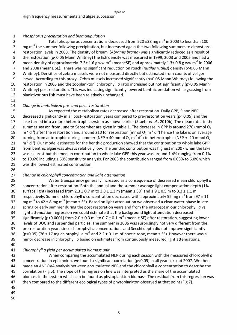
High frequency measurements and algae succession

8

Phosphorus precipitation and biomanipulation 1 Total phosphorus concentrations decreased from 220 ±38 mg m-3 in 2003 to less than 100 2

mg m-3 the summer following precipitation, but increased again the two following summers to almost pre-3 restoration levels in 2008. The density of bream (Abramis brama) was significantly reduced as a result of 4 the restoration (p<0.05 Mann Whitney) the fish density was measured in 1999, 2003 and 2005 and had a 5 mean density of approximately 7.3± 1.6 g ww m-2 (mean±SE) and approximately 1.3± 0.8 g ww m-2 in 2006 6 and 2008 (mean± SE). There was no significant reduction on roach (Rutilus rutilus) density (p>0.05 Mann 7 Whitney). Densities of zebra mussels were not measured directly but estimated from counts of veliger 8 larvae. According to this proxy, Zebra mussels increased significantly (p<0.05 Mann Whitney) following the 9 restoration in 2005 and the zooplankton: chlorophyll a ratio increased but not significantly (p>0.05 Mann 10 Whitney) post restoration. This was indicating significantly lowered benthic predation while grassing from 11 planktivorious fish must have been relatively unchanged. 12 13 Change in metabolism pre- and post- restoration 14

As expected the metabolism rates decreased after restoration. Daily GPP, R and NEP 15 decreased significantly in all post-restoration years compared to pre-restoration years (p< 0.05) and the 16 lake turned into a more heterotrophic system as shown earlier (Staehr et al., 2010b). The mean rates in the 17 summer season from June to September are given in table 1. The decrease in GPP is around 270 (mmol O2 18 m-2 d-1) after the restoration and around 210 for respiration (mmol O2 m-2 d-1) hence the lake is on average 19 turning from autotrophic during summer (NEP ≈ 40 mmol O2 m-2 d-1) to heterotrophic (NEP ≈ -20 mmol O2 20 m-2 d-1). Our model estimates for the benthic production showed that the contribution to whole lake GPP 21 from benthic algae was always relatively low. The benthic contribution was highest in 2007 when the lake 22 was clearest but the median contribution to whole lake GPP this year was around 1.4% ranging from 0.1% 23 to 10.6% including ± 50% sensitivity analysis. For 2003 the contribution ranged from 0.03% to 6.0% which 24 was the lowest estimated contribution. 25 26 Change in chlorophyll concentration and light attenuation 27

Water transparency generally increased as a consequence of decreased mean chlorophyll a 28 concentration after restoration. Both the annual and the summer average light compensation depth (1% 29 surface light) increased from 2.3 ± 0.7 m to 3.8 ± 1.3 m (mean ± SD) and 1.9 ± 0.5 m to 3.3 ± 1.1 m 30 respectively. Summer chlorophyll a concentration decreased with approximately 55 mg m-3 from 97 ± 11 31 mg m-3 to 42 ± 8 mg m-3 (mean ± SE). Based on light attenuation we observed a clear-water phase in late 32 spring or early summer during the post restoration years and from the intercept in our chlorophyll a vs. 33 light attenuation regression we could estimate that the background light attenuation decreased 34 significantly (p<0.0001) from 2.0 ± 0.3 m-1 to 0.7 ± 0.1 m-1 (mean ± SE) after restoration, suggesting lower 35 levels of DOC and suspended particles. The summer in 2006 was surprisingly not very different from the 36 pre-restoration years since chlorophyll a concentrations and Secchi depth did not improve significantly 37 (p>0.05) (76 ± 17 mg chlorophyll a m-3 and 2.2 ± 0.1 m of photic zone, mean ± SE). However there was a 38 minor decrease in chlorophyll a based on estimates from continuously measured light attenuations. 39 40 Chlorophyll a yield per accumulated biomass unit 41

When comparing the accumulated NEP during each season with the measured chlorophyll a 42 concentration in epilimnion, we found a significant correlation (p<0.05) in all years except 2007. We then 43 made an ANCOVA analysis between accumulated NEP and the chlorophyll a concentration to describe the 44 correlation (Fig 5). The slope of this regression line was interpreted as the share of the accumulated 45 biomass in the system which can be found as phytoplankton biomass. The residual from this regression was 46 then compared to the different ecological types of phytoplankton observed at that point (Fig 7). 47 48 49 50

Paper IV

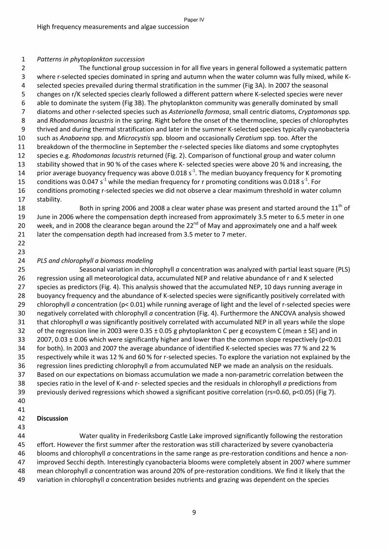
High frequency measurements and algae succession

9

Patterns in phytoplankton succession 1 The functional group succession in for all five years in general followed a systematic pattern 2

where r-selected species dominated in spring and autumn when the water column was fully mixed, while K-3 selected species prevailed during thermal stratification in the summer (Fig 3A). In 2007 the seasonal 4 changes on r/K selected species clearly followed a different pattern where K-selected species were never 5 able to dominate the system (Fig 3B). The phytoplankton community was generally dominated by small 6 diatoms and other r-selected species such as Asterionella formosa, small centric diatoms, Cryptomonas spp. 7 and Rhodomonas lacustris in the spring. Right before the onset of the thermocline, species of chlorophytes 8 thrived and during thermal stratification and later in the summer K-selected species typically cyanobacteria 9 such as Anabaena spp. and Microcystis spp. bloom and occasionally Ceratium spp. too. After the 10 breakdown of the thermocline in September the r-selected species like diatoms and some cryptophytes 11 species e.g. Rhodomonas lacustris returned (Fig. 2). Comparison of functional group and water column 12 stability showed that in 90 % of the cases where K- selected species were above 20 % and increasing, the 13 prior average buoyancy frequency was above 0.018 s-1. The median buoyancy frequency for K promoting 14 conditions was 0.047 s-1 while the median frequency for r promoting conditions was 0.018 s-1. For 15 conditions promoting r-selected species we did not observe a clear maximum threshold in water column 16 stability. 17

Both in spring 2006 and 2008 a clear water phase was present and started around the 11th of 18 June in 2006 where the compensation depth increased from approximately 3.5 meter to 6.5 meter in one 19 week, and in 2008 the clearance began around the 22nd of May and approximately one and a half week 20 later the compensation depth had increased from 3.5 meter to 7 meter. 21

22 23 PLS and chlorophyll a biomass modeling 24

Seasonal variation in chlorophyll a concentration was analyzed with partial least square (PLS) 25 regression using all meteorological data, accumulated NEP and relative abundance of r and K selected 26 species as predictors (Fig. 4). This analysis showed that the accumulated NEP, 10 days running average in 27 buoyancy frequency and the abundance of K-selected species were significantly positively correlated with 28 chlorophyll a concentration (p< 0.01) while running average of light and the level of r-selected species were 29 negatively correlated with chlorophyll a concentration (Fig. 4). Furthermore the ANCOVA analysis showed 30 that chlorophyll a was significantly positively correlated with accumulated NEP in all years while the slope 31 of the regression line in 2003 were 0.35 ± 0.05 g phytoplankton C per g ecosystem C (mean ± SE) and in 32 2007, 0.03 ± 0.06 which were significantly higher and lower than the common slope respectively (p<0.01 33 for both). In 2003 and 2007 the average abundance of identified K-selected species was 77 % and 22 % 34 respectively while it was 12 % and 60 % for r-selected species. To explore the variation not explained by the 35 regression lines predicting chlorophyll a from accumulated NEP we made an analysis on the residuals. 36 Based on our expectations on biomass accumulation we made a non-parametric correlation between the 37 species ratio in the level of K-and r- selected species and the residuals in chlorophyll a predictions from 38 previously derived regressions which showed a significant positive correlation (rs=0.60, p<0.05) (Fig 7). 39 40 41 Discussion 42

43 Water quality in Frederiksborg Castle Lake improved significantly following the restoration 44

effort. However the first summer after the restoration was still characterized by severe cyanobacteria 45 blooms and chlorophyll a concentrations in the same range as pre-restoration conditions and hence a non-46 improved Secchi depth. Interestingly cyanobacteria blooms were completely absent in 2007 where summer 47 mean chlorophyll a concentration was around 20% of pre-restoration conditions. We find it likely that the 48 variation in chlorophyll a concentration besides nutrients and grazing was dependent on the species 49

Paper IV

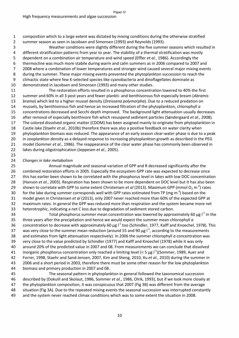
High frequency measurements and algae succession

10

composition which to a large extent was dictated by mixing conditions during the otherwise stratified 1 summer season as seen in Jacobsen and Simonsen (1993) and Reynolds (1993). 2

Weather conditions were slightly different during the five summer seasons which resulted in 3 different stratification patterns from year to year. The stability of a thermal stratification was mostly 4 dependent on a combination air temperature and wind speed (Effler et al., 1986). Accordingly the 5 thermocline was much more stabile during warm and calm summers as in 2006 compared to 2007 and 6 2008 where a combination of lower temperatures and stronger wind caused several major mixing events 7 during the summer. These major mixing events prevented the phytoplankton succession to reach the 8 climactic state where few K-selected species like cyanobacteria and dinoflagellates dominate as 9 demonstrated in Jacobsen and Simonsen (1993) and many other studies. 10

The restoration efforts resulted in a phosphorus concentration lowered to 40% the first 11 summer and 60% in all 3 post years and fewer plankti- and benthivorous fish especially bream (Abramis 12 brama) which led to a higher mussel density (Dreissena polymorpha). Due to a reduced predation on 13 mussels, by benthivorous fish and hence an increased filtration of the phytoplankton, chlorophyll a 14 concentrations decreased and Secchi depth improved. The background light attenuation usually decreases 15 after removal of especially benthivore fish which resuspend sediment particles (Søndergaard et al., 2008). 16 The colored dissolved organic matter (CDOM) has been assigned mainly to originate from phytoplankton in 17 Castle lake (Staehr et al., 2010b) therefore there was also a positive feedback on water clarity when 18 phytoplankton biomass was reduced. The appearance of an early season clear-water phase is due to a peak 19 in zooplankton density as a delayed response to increasing phytoplankton growth as described in the PEG 20 model (Sommer et al., 1986). The reappearance of the clear water phase has commonly been observed in 21 lakes during oligotrophication (Jeppesen et al., 2005). 22 23 Changes in lake metabolism 24 Annual magnitude and seasonal variation of GPP and R decreased significantly after the 25 combined restoration efforts in 2005. Especially the ecosystem GPP rate was expected to decrease since 26 this has earlier been shown to be correlated with the phosphorus level in lakes with low DOC concentration 27 (Hanson et al., 2003). Respiration has been shown to be more dependent on DOC level but it has also been 28 shown to correlate with GPP to some extent Christensen et al (2013). Maximum GPP (mmol O2 m-2) rates 29 for the lake during summer corresponds well with GPP rates estimated from TP (mg m-3) based on the 30 model given in Christensen et al (2013), only 2007 never reached more than 60% of the expected GPP at 31 maximum rates. In general the GPP was reduced more than respiration and the system became more net 32 heterotrophic, indicating a net C loss due to degradation of sediment stored carbon. 33

Total phosphorus summer mean concentration was lowered by approximately 60 µg l-1 in the 34 three years after the precipitation and hence we would expect the summer mean chlorophyll a 35 concentration to decrease with approximately 60 µg l-1 too (Schindler, 1977, Kalff and Knoechel, 1978). This 36 was very close to the summer mean reduction (around 55 and 90 µg l-1, according to the measurements 37 and estimates from light attenuation respectively). In 2006 the summer chlorophyll a concentration was 38 very close to the value predicted by Schindler (1977) and Kalff and Knoechel (1978) while it was only 39 around 20% of the predicted value in 2007 and 08. From measurements we can conclude that dissolved 40 inorganic phosphorus concentration only reached a limiting level (< 5 µg l-1)(Sommer, 1989, Auer and 41 Forrer, 1998, Staehr and Sand-Jensen, 2007, Kim and Sheng, 2010, Xu et al., 2010) during the summer in 42 2006 and a short period in 2003, therefore there must be some other reason for the low phytoplankton 43 biomass and primary production in 2007 and 08. 44

The seasonal pattern in phytoplankton in general followed the taxonomical succession 45 described by (Dokulil and Skolaut, 1986, Sommer et al., 1986, Olrik, 1993), but if we look more closely at 46 the phytoplankton composition, it was conspicuous that 2007 (Fig 3B) was different from the average 47 situation (Fig 3A). Due to the repeated mixing events the seasonal succession was interrupted constantly 48 and the system never reached climax conditions which was to some extent the situation in 2008. 49

Paper IV

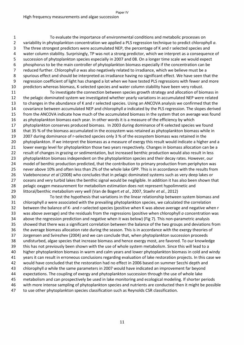
High frequency measurements and algae succession

11

To evaluate the importance of environmental conditions and metabolic processes on 1 variability in phytoplankton concentration we applied a PLS regression technique to predict chlorophyll a. 2 The three strongest predictors were accumulated NEP, the percentage of K and r selected species and 3 water column stability. Surprisingly, TP was not a strong predictor, which we interpret as a consequence of 4 succession of phytoplankton species especially in 2007 and 08. On a longer time scale we would expect 5 phosphorus to be the main controller of phytoplankton biomass especially if the concentration can be 6 reduced further. Chlorophyll a was also negatively related to irradiance, which we believe must be a 7 spurious effect and should be interpreted as irradiance having no significant effect. We have seen that the 8 regression coefficient of light has changed a lot when we have tested PLS regressions with fewer and more 9 predictors whereas biomass, K-selected species and water column stability have been very robust. 10

To investigate the connection between species growth strategy and allocation of biomass in 11 the pelagic dominated system we investigated whether yearly variations in accumulated NEP were related 12 to changes in the abundance of K and r selected species. Using an ANCOVA analysis we confirmed that the 13 covariance between accumulated NEP and chlorophyll a indicated by the PLS regression. The slopes derived 14 from the ANCOVA indicate how much of the accumulated biomass in the system that on average was found 15 as phytoplankton biomass each year. In other words it is a measure of the efficiency by which 16 phytoplankton conserves produced biomass. In 2003 during dominance of K-selected species we found 17 that 35 % of the biomass accumulated in the ecosystem was retained as phytoplankton biomass while in 18 2007 during dominance of r-selected species only 3 % of the ecosystem biomass was retained in the 19 phytoplankton. If we interpret the biomass as a measure of exergy this result would indicate a higher and a 20 lower exergy level for phytoplankton those two years respectively. Changes in biomass allocation can be a 21 result of changes in grazing or sedimentation, but increased benthic production would also result in less 22 phytoplankton biomass independent on the phytoplankton species and their decay rates. However, our 23 model of benthic production predicted, that the contribution to primary production from periphyton was 24 never above 10% and often less than 2% of the whole lake GPP. This is in accordance with the results from 25 Vadeboncoeur et al (2008) who concludes that in pelagic dominated systems such as very deep lakes or 26 oceans and very turbid lakes the benthic signal would be negligible. In addition it has also been shown that 27 pelagic oxygen measurement for metabolism estimation does not represent hypolimnetic and 28 littoral/benthic metabolism very well (Van de Bogert et al., 2007, Staehr et al., 2012) 29

To test the hypothesis that variations in the linear relationship between system biomass and 30 chlorophyll a were associated with the prevailing phytoplankton species, we calculated the correlation 31 between the balance of K- and r-selected species (positive when K was above average and negative when r 32 was above average) and the residuals from the regressions (positive when chlorophyll a concentration was 33 above the regression prediction and negative when it was below) (Fig 7). This non-parametric analysis 34 showed that there was a significant correlation between the balance of the two groups and deviations from 35 the average biomass allocation rate during the season. This is in accordance with the exergy theories of 36 Jorgensen and Svirezhev (2004) and we can conclude that, when phytoplankton succession proceeds 37 undisturbed, algae species that increase biomass and hence exergy most, are favored. To our knowledge 38 this has not previously been shown with the use of whole system metabolism. Since this will lead to a 39 higher phytoplankton biomass in warm and calm years and lower phytoplankton biomass in cold and windy 40 years it can result in erroneous conclusions regarding evaluation of lake restoration projects. In this case we 41 would have concluded that the restoration had no effect in 2006 based on summer Secchi depth and 42 chlorophyll a while the same parameters in 2007 would have indicated an improvement far beyond 43 expectations. The coupling of exergy and phytoplankton succession through the use of whole lake 44 metabolism and can prospectively be used in lake monitoring and ecological modeling. If shorter periods 45 with more intense sampling of phytoplankton species and nutrients are conducted then it might be possible 46 to use other phytoplankton species classification such as Reynolds CSR classification. 47

Paper IV

High frequency measurements and algae succession

12

Acknowledgements 1 This study was financially supported by the Villum Kann Rasmussen Centre of Excellence Centre for Lake 2 Restoration (CLEAR), The Danish Strategic Research Council supported who the project “Monitoring remote 3 environments with Autonomous sensor Network-based data Acquisition" (MANA) and Frederiksborg 4 County, Denmark. The authors would like to thank lab technicians and students who have been involved in 5 the sampling and processing of data, and thanks to Dr Alex Elliott from Centre for Ecology & Hydrology, 6 Lancaster for comments. 7 8

Paper IV

High frequency measurements and algae succession

13

References 1 2

Andersen, J., Jacobsen, O., Grevy, P. & Markmann, P. (1979) Production and decomposition of organic 3 matter in eutrophic Frederiksborg Slotssø, Denmark. Arch. Hydrobiol, 85, 511-542. 4

Auer, M.T. & Forrer, B. (1998) Development and Parameterization of a Kinetic Framework for Modeling 5 Light- and Phosphorus- Limited Phytoplankton Growth in Cannonsville Reservoir. Lake and 6 Reservoir Management, 14, 290-300. 7

Bjørn, C. (2005) Fiskebestanden i Frederiksborg Slotssø. 8 9 Cazzanelli, M., Warming, T. & Christoffersen, K. (2008) Emergent and floating-leaved macrophytes as 10

refuge for zooplankton in a eutrophic temperate lake without submerged vegetation. 11 Hydrobiologia, 605, 113-122. 12

Cole, J.J. & Caraco, N.F. (1998) Atmospheric exchange of carbon dioxide in a low-wind oligotrophic lake 13 measured by the addition of SF6. Limnology and Oceanography, 43, 647-656. 14

Dokulil, M. & Skolaut, C. (1986) Succession of phytoplankton in a deep stratifying lake: Mondsee, Austria. 15 Hydrobiologia, 138, 9-24. 16

Effler, S., Owens, E., Schimel, K. & Dobi, J. (1986) Weather-Based Variations in Thermal Stratification. 17 Journal of Hydraulic Engineering, 112, 159-165. 18

Egemose, S., Jensen, H.S. & Reitzel, K. (2011) Erfaringer med aluminiumbehandling af danske søer. 19 Miljøministeriet, Naturstyrelsen. 20

21 Egemose, S., Reitzel, K., Andersen, F. & Jensen, H. (2012) Resuspension-mediated aluminium and 22

phosphorus distribution in lake sediments after aluminium treatment. Hydrobiologia, 701, 79-88. 23 Hansen, A., Jeppesen, E., Bosselmann, S. & Andersen, P. (1992) Zooplankton i søer–metoder og artsliste, 24

Miljøprojekt nr. 205. Miljøstyrelsen, Copenhagen. 25 Hanson, P.C., Bade, D.L., Carpenter, S.R. & Kratz, T.K. (2003) Lake metabolism: relationships with 26

dissolved organic carbon and phosphorus. Limnology and Oceanography, 48, 1112-1119. 27 Hanson, P.C., Carpenter, S.R., Kimura, N., Wu, C., Cornelius, S.P. & Kratz, T.K. (2008) Evaluation of 28

metabolism models for free-water dissolved oxygen methods in lakes. Limnology and 29 Oceanography-Methods, 6, 454-465. 30

Imberger, J. & Patterson, J.C. (1989) Physical Limnology. In: Advances in Applied Mechanics. pp. 303-475. 31 Elsevier. 32

Jacobsen, B. & Simonsen, P. (1993) Disturbance events affecting phytoplankton biomass, composition 33 and species diversity in a shallow, eutrophic, temperate lake. Hydrobiologia, 249, 9-14. 34

Jahne, B., Heinz, G. & Dietrich, W. (1987) Measurement of the diffusion-coefficients of sparingly soluble 35 gases in water. Journal of Geophysical Research-Oceans, 92, 10767-10776. 36

Jennings, E., Jones, S., Arvola, L., Staehr, P.A., Gaiser, E., Jones, I.D., Weathers, K.C., Weyhenmeyer, G.A., 37 Chiu, C.-Y. & De Eyto, E. (2012) Effects of weather-related episodic events in lakes: an analysis 38 based on high-frequency data. Freshwater Biology, 57, 589-601. 39

Jeppesen, E., Søndergaard, M., Jensen, J.P., Havens, K.E., Anneville, O., Carvalho, L., Coveney, M.F., 40 Deneke, R., Dokulil, M.T., Foy, B.O.B., Gerdeaux, D., Hampton, S.E., Hilt, S., Kangur, K., Köhler, 41 J.a.N., Lammens, E.H.H.R., Lauridsen, T.L., Manca, M., Miracle, M.R., Moss, B., Nõges, P., Persson, 42 G., Phillips, G., Portielje, R.O.B., Romo, S., Schelske, C.L., Straile, D., Tatrai, I., Willén, E.V.A. & 43 Winder, M. (2005) Lake responses to reduced nutrient loading – an analysis of contemporary 44 long-term data from 35 case studies. Freshwater Biology, 50, 1747-1771. 45

Jespersen, A. & Christoffersen, K. (1987) Measurements of chlorophyll-a from phytoplankton using 46 ethanol as extraction solvent. Archiv fur Hydrobiologie. Stuttgart, 109, 445-454. 47

Jørgensen, S.E. (1992) Exergy and ecology. Ecological Modelling, 63, 185-214. 48 Jorgensen, S.E. & Bendoricchio, G. (2001) Fundamentals of Ecological Modelling. Third edition Elsevier, 49

Amsterdam. 50

Paper IV

High frequency measurements and algae succession

14

Jorgensen, S.E. & Svirezhev, Y.M. (2004) Towards a thermodynamic theory for ecological systems 1 Pergamon. 2

Kalff, J. & Knoechel, R. (1978) Phytoplankton and their Dynamics in Oligotrophic and Eutrophic Lakes. 3 Annual Review of Ecology and Systematics, 9, 475-495. 4

Kim, T. & Sheng, Y.P. (2010) Estimation of water quality model parameters. KSCE Journal of Civil 5 Engineering, 14, 421-437. 6

Kõiv, T. & Kangro, K. (2005) Resource Ratios and Phytoplankton Species Composition in a Strongly 7 Stratified Lake. Hydrobiologia, 547, 123-135. 8

Lewis, W., Jr. (1986) Phytoplankton succession in Lake Valencia, Venezuela. Hydrobiologia, 138, 189-203. 9 Lindenschmidt, K.-E. & Chorus, I. (1998) The effect of water column mixing on phytoplankton succession, 10

diversity and similarity. Journal of Plankton Research, 20, 1927-1951. 11 Macarthur, R. & Levins, R. (1967) The Limiting Similarity, Convergence, and Divergence of Coexisting 12

Species. The American Naturalist, 101, 377-385. 13 Macintyre, S., Flynn, K.M., Jellison, R. & Romero, J.R. (1999) Boundary Mixing and Nutrient Fluxes in 14

Mono Lake, California. Limnology and Oceanography, 44, 512-529. 15 Odum, H.T. (1956) Primary production in flowing waters. Limnology and Oceanography, 1, 102-117. 16 Olrik, K. (1993) Planteplankton - økologi: økologiske faktorer for planteplankton i søer og marine 17

områder, p. 165 Miljøstyrelsen. 18 Rasmussen, H.U. (2001) Frederiksborg Slotssø 1999. Hillerød. 19 20 Ray, S., Berec, L., Straškraba, M. & Jørgensen, S.E. (2001) Optimization of exergy and implications of body 21

sizes of phytoplankton and zooplankton in an aquatic ecosystem model. Ecological Modelling, 22 140, 219-234. 23

Read, J.S., Hamilton, D.P., Jones, I.D., Muraoka, K., Winslow, L.A., Kroiss, R., Wu, C.H. & Gaiser, E. (2011) 24 Derivation of lake mixing and stratification indices from high-resolution lake buoy data. 25 Environmental Modelling & Software, 26, 1325-1336. 26

Reynolds, C. (1993) Scales of disturbance and their role in plankton ecology. Hydrobiologia, 249, 157-171. 27 Reynolds, C.S. (1980) Phytoplankton assemblages and their periodicity in stratifying lake systems. 28

Holarctic Ecology, 3, 141-159. 29 Reynolds, C.S. (2002) Ecological pattern and ecosystem theory. Ecological Modelling, 158, 181-200. 30 Reynolds, C.S., Padisák, J. & Sommer, U. (1993) Intermediate disturbance in the ecology of phytoplankton 31

and the maintenance of species diversity: a synthesis. Hydrobiologia, 249, 183-188. 32 Schindler, D. (1977) Evolution of phosphorus limitation in lakes. Science, 195, 260-262. 33 Silow, E.A. & Mokry, A.V. (2010) Exergy as a Tool for Ecosystem Health Assessment. Entropy, 12, 902-925. 34 Skaarup, P., Jørgensen, P.B., Rasmussen, J. & Gabriel, S. (2006) Restaurering af Frederiksborg Slotssø. In: 35

Stads- og havneingeniøren. pp. 45-46 36 Sommer, U. (1989) Nutrient status and nutrient competition of phytoplankton in a shallow, hypertrophic 37

lake. Limnology and Oceanography, 34, 1162-1173. 38 Sommer, U., Gliwicz, Z.M., Lampert, W. & Duncan, A. (1986) PEG-model of seasonal succession of 39

planktonic events in fresh waters. Archiv fuer Hydrobiologie AHYBAY, 106. 40 Søndergaard, M., Liboriussen, L., Pedersen, A. & Jeppesen, E. (2008) Lake Restoration by Fish Removal: 41

Short- and Long-Term Effects in 36 Danish Lakes. Ecosystems, 11, 1291-1305. 42 Staehr, P.A., Bade, D., Van De Bogert, M.C., Koch, G.R., Williamson, C., Hanson, P., Cole, J.J. & Kratz, T. 43

(2010a) Lake metabolism and the diel oxygen technique: State of the science. Limnology and 44 Oceanography: Methods, 8, 628-644. 45

Staehr, P.A., Christensen, J.P.A., Batt, R.D. & Read, J.S. (2012) Ecosystem metabolism in a stratified lake. 46 Limnol. Oceanogr, 57, 1317-1330. 47

Staehr, P.A. & Sand-Jensen, K. (2007) Temporal dynamics and regulation of lake metabolism. Limnology 48 and Oceanography, 52, 108-120. 49

Paper IV

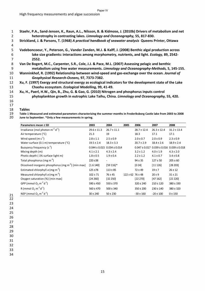
High frequency measurements and algae succession

15

Staehr, P.A., Sand-Jensen, K., Raun, A.L., Nilsson, B. & Kidmose, J. (2010b) Drivers of metabolism and net 1 heterotrophy in contrasting lakes. Limnology and Oceanography, 55, 817-830. 2

Strickland, J. & Parsons, T. (1968) A practical handbook of seawater analysis Queens Printer, Ottawa 3 4 Vadeboncoeur, Y., Peterson, G., Vander Zanden, M.J. & Kalff, J. (2008) Benthic algal production across 5

lake size gradients: interactions among morphometry, nutrients, and light. Ecology, 89, 2542-6 2552. 7

Van De Bogert, M.C., Carpenter, S.R., Cole, J.J. & Pace, M.L. (2007) Assessing pelagic and benthic 8 metabolism using free water measurements. Limnology and Oceanography-Methods, 5, 145-155. 9

Wanninkhof, R. (1992) Relationship between wind-speed and gas-exchange over the ocean. Journal of 10 Geophysical Research-Oceans, 97, 7373-7382. 11

Xu, F. (1997) Exergy and structural exergy as ecological indicators for the development state of the Lake 12 Chaohu ecosystem. Ecological Modelling, 99, 41-49. 13

Xu, H., Paerl, H.W., Qin, B., Zhu, G. & Gao, G. (2010) Nitrogen and phosphorus inputs control 14 phytoplankton growth in eutrophic Lake Taihu, China. Limnology and Oceanography, 55, 420. 15

16 17 Tables 18 Table 1 Measured and estimated parameters characterizing the summer months in Frederiksborg Castle lake from 2003 to 2008 19 June to September. *Only a few measurements in spring. 20

21 22 23 24 25 26 27 28 29 30 31 32 33 34

Parameters mean ± SD 2003 2004 2005 2006 2007 2008Irradiance (mol photon m-2 d-1) 29.6 ± 11.3 26.7 ± 11.1 28.7 ± 12.4 26.3 ± 12.4 31.2 ± 13.4Air temperature (°C) 21.3 19 18.3 17.1 17.1Wind speed (m s-1) 2.8 ± 1.1 2.5 ± 0.9 2.0 ± 0.7 2.0 ± 0.9 2.3 ± 0.9Water surface (0.1 m) temperature (°C) 19.5 ± 2.4 18.3 ± 3.3 20.7 ± 2.9 18.4 ± 2.6 18.9 ± 2.4 Buoyancy frequency (s-1) 0.044 ± 0.015 0.034 ± 0.014 0.047 ± 0.017 0.039 ± 0.016 0.039 ± 0.018Mixing depth (m) 4.1 ± 2.1 4.3 ± 2.4 3.2 ± 1.2 4.0 ± 1.9 4.3 ± 2.0Photic depth ( 1% surface light m) 1.8 ± 0.5 1.9 ± 0.4 2.2 ± 1.2 4.1 ± 0.7 3.4 ± 0.8Total phosphorus (mg m-3) 220 ±38 - 94 ± 35 127 ± 50 205 ± 60Dissolved inorganic phosphorus (mg m-3) [min max] [1.6 140] [59 116]* [0 24] [11 126] [28 203]Estimated chlorphyll a (mg m-3) 125 ±78 113 ± 85 72 ± 49 19 ± 7 26 ± 12Measured chlorphyll a (mg m-3) 102 ± 71 76 ± 45 122 ± 62 76 ± 48 20 ± 9 31 ± 21Oxygen saturation (%) [min max] [24 260] [32 250] [22 270] [47 162] [22 220]GPP (mmol O2 m-2 d-1) 590 ± 450 550 ± 370 320 ± 240 210 ± 120 380 ± 330

R (mmol O2 m-2 d-1) 560 ± 470 500 ± 340 350 ± 200 230 ± 140 380 ± 320

NEP (mmol O2 m-2 d-1) 30 ± 240 50 ± 230 -30 ± 160 -20 ± 100 0 ± 150

Paper IV

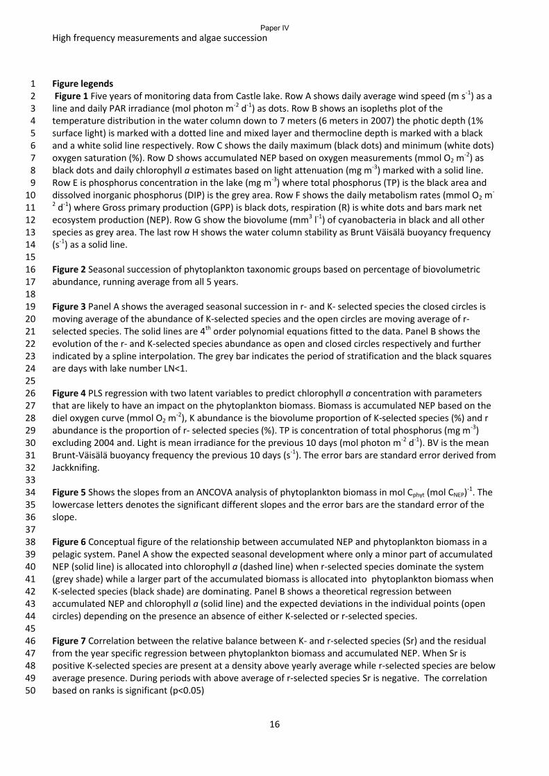
High frequency measurements and algae succession

16

Figure legends 1 Figure 1 Five years of monitoring data from Castle lake. Row A shows daily average wind speed (m s-1) as a 2 line and daily PAR irradiance (mol photon m-2 d-1) as dots. Row B shows an isopleths plot of the 3 temperature distribution in the water column down to 7 meters (6 meters in 2007) the photic depth (1% 4 surface light) is marked with a dotted line and mixed layer and thermocline depth is marked with a black 5 and a white solid line respectively. Row C shows the daily maximum (black dots) and minimum (white dots) 6 oxygen saturation (%). Row D shows accumulated NEP based on oxygen measurements (mmol O2 m-2) as 7 black dots and daily chlorophyll a estimates based on light attenuation (mg m-3) marked with a solid line. 8 Row E is phosphorus concentration in the lake (mg m-3) where total phosphorus (TP) is the black area and 9 dissolved inorganic phosphorus (DIP) is the grey area. Row F shows the daily metabolism rates (mmol O2 m-10 2 d-1) where Gross primary production (GPP) is black dots, respiration (R) is white dots and bars mark net 11 ecosystem production (NEP). Row G show the biovolume (mm3 l-1) of cyanobacteria in black and all other 12 species as grey area. The last row H shows the water column stability as Brunt Väisälä buoyancy frequency 13 (s-1) as a solid line. 14 15 Figure 2 Seasonal succession of phytoplankton taxonomic groups based on percentage of biovolumetric 16 abundance, running average from all 5 years. 17 18 Figure 3 Panel A shows the averaged seasonal succession in r- and K- selected species the closed circles is 19 moving average of the abundance of K-selected species and the open circles are moving average of r-20 selected species. The solid lines are 4th order polynomial equations fitted to the data. Panel B shows the 21 evolution of the r- and K-selected species abundance as open and closed circles respectively and further 22 indicated by a spline interpolation. The grey bar indicates the period of stratification and the black squares 23 are days with lake number LN<1. 24 25 Figure 4 PLS regression with two latent variables to predict chlorophyll a concentration with parameters 26 that are likely to have an impact on the phytoplankton biomass. Biomass is accumulated NEP based on the 27 diel oxygen curve (mmol O2 m-2), K abundance is the biovolume proportion of K-selected species (%) and r 28 abundance is the proportion of r- selected species (%). TP is concentration of total phosphorus (mg m-3) 29 excluding 2004 and. Light is mean irradiance for the previous 10 days (mol photon m-2 d-1). BV is the mean 30 Brunt-Väisälä buoyancy frequency the previous 10 days (s-1). The error bars are standard error derived from 31 Jackknifing. 32 33 Figure 5 Shows the slopes from an ANCOVA analysis of phytoplankton biomass in mol Cphyt (mol CNEP)-1. The 34 lowercase letters denotes the significant different slopes and the error bars are the standard error of the 35 slope. 36 37 Figure 6 Conceptual figure of the relationship between accumulated NEP and phytoplankton biomass in a 38 pelagic system. Panel A show the expected seasonal development where only a minor part of accumulated 39 NEP (solid line) is allocated into chlorophyll a (dashed line) when r-selected species dominate the system 40 (grey shade) while a larger part of the accumulated biomass is allocated into phytoplankton biomass when 41 K-selected species (black shade) are dominating. Panel B shows a theoretical regression between 42 accumulated NEP and chlorophyll a (solid line) and the expected deviations in the individual points (open 43 circles) depending on the presence an absence of either K-selected or r-selected species. 44 45 Figure 7 Correlation between the relative balance between K- and r-selected species (Sr) and the residual 46 from the year specific regression between phytoplankton biomass and accumulated NEP. When Sr is 47 positive K-selected species are present at a density above yearly average while r-selected species are below 48 average presence. During periods with above average of r-selected species Sr is negative. The correlation 49 based on ranks is significant (p<0.05) 50

Paper IV

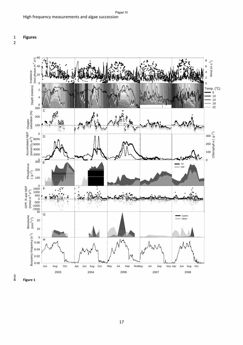
High frequency measurements and algae succession

17

Figures 1 2

3 Figure 1 4

X Data

Jun Jul Aug Sep Oct Nov

Phos

phor

us(

g l-1

)

0

100

200

300

X Data

Apr Jun Aug Oct

TPDIP

X Data

May Jun Jul Aug Sep Oct Nov

X Data

Apr Jun Aug Oct

X Data

May Jun Jul Aug Sep Oct Nov

GPP

, R a

nd N

EP

(mm

ol m

-2 d

-1)

-1500-1000

-500

50010001500

0

X Data

Jun Jul Aug Sep Oct Nov

Dep

th (m

eter

s)

2

4

6Apr Jun Aug Oct

X Data

May Jun Jul Aug Sep Oct Nov Apr Jun Aug Oct

6 10 14 18 22

Irrad

ianc

e(m

ol p

hoto

n m

-2 d

-1)

0

20

40

60

Win

d (m

s-1

)

0

2

4

6

8

Accu

mul

ated

NEP

(m

mol

O2

m-3

)

0

2000

4000

6000

8000

Chl

orop

hyll

a (

g l-1

)

0

100

200

300

X Data

Jun Jul Aug Sep Oct Nov

Biov

olum

e (m

m3 l-1

)

0

10

20

30

X Data

Apr Jun Aug Oct

X Data

May Jun Jul Aug Sep Oct Nov

X Data

Apr Jun Aug Oct

Cyano Other

X Data

May Jun Jul Aug Sep Oct Nov

2003

Jun Aug Oct Buoy

ancy

freq

uenc

y (s

-1)

0.00

0.02

0.04

0.06

2004

Apr Jun Aug Oct

2006

May Jul Sep Nov

2008

Apr Jun Aug Oct

2007

May Jul Sep Nov

Oxy

gen

satu

ratio

n (%

)

0

200

300

100

Temp. (oC)

A

B

C

D

E

F

G

H

Paper IV

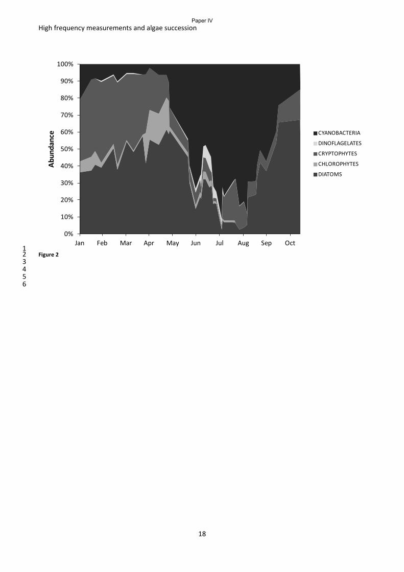
High frequency measurements and algae succession

18

1 Figure 2 2 3 4 5 6

0%

10%

20%

30%

40%

50%

60%

70%

80%

90%

100%

Jan Feb Mar Apr May Jun Jul Aug Sep Oct

Abun

danc

e CYANOBACTERIA

DINOFLAGELATES

CRYPTOPHYTES

CHLOROPHYTES

DIATOMS

Paper IV

High frequency measurements and algae succession

19

1 Figure 3 2

0

20

40

60

80

100

Feb Mar May Jun Aug Oct

Abu

ndan

ce (%

)

K

r

Stratifed

0

20

40

60

80

100

Feb-07 Mar-07 May-07 Jul-07 Aug-07 Oct-07

Abu

ndan

ce (%

)

K

r

Stratifed

A

B

Paper IV

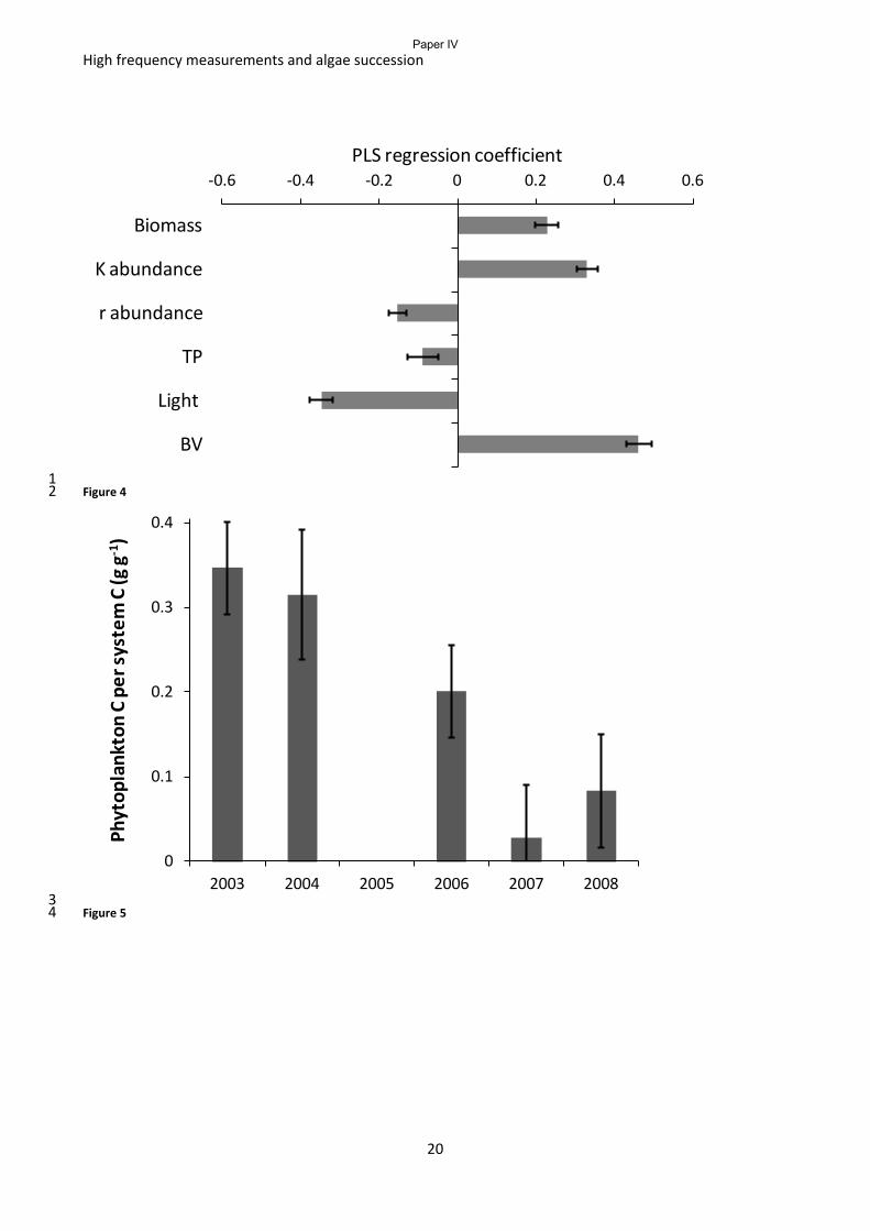
High frequency measurements and algae succession

20

1 Figure 4 2

3 Figure 5 4

-0.6 -0.4 -0.2 0 0.2 0.4 0.6

Biomass

K abundance

r abundance

TP

Light

BV

PLS regression coefficient

0

0.1

0.2

0.3

0.4

2003 2004 2005 2006 2007 2008

Phyt

opla

nkto

n C

per s

yste

m C

(g g

-1)

Paper IV

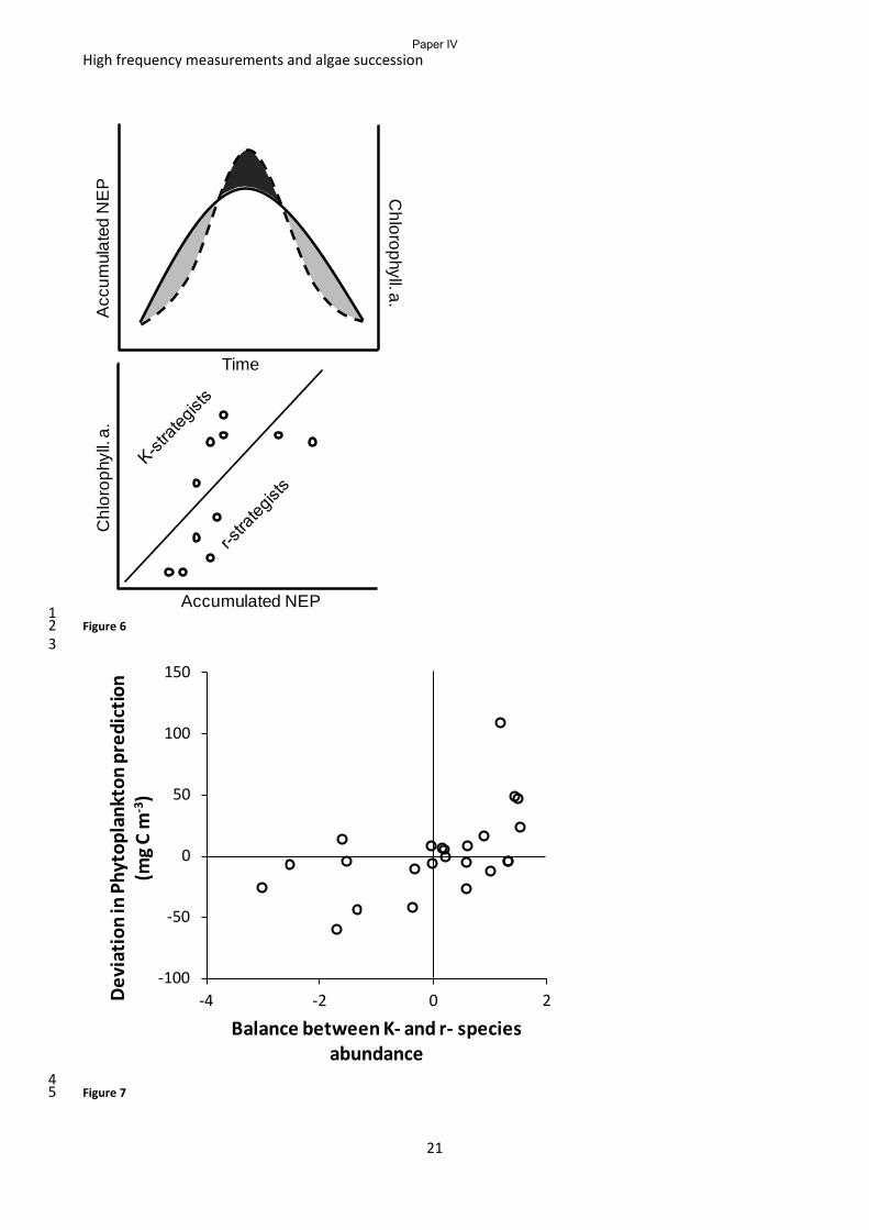
High frequency measurements and algae succession

21

1 Figure 6 2 3

4 Figure 7 5

Acc

umul

ated

NE

P Chlorophyll. a.

Time

Accumulated NEP

Chl

orop

hyll.

a.

-100

-50

0

50

100

150

-4 -2 0 2Devi

atio

n in

Phy

topl

ankt

on p

redi

ctio

n (m

g C m

-3)

Balance between K- and r- species abundance

Paper IV

104

Acknowledgements

Thanks to all the people who supported me during the past three years, especially my patient family

who did not leave me despite a compressed program and several weeks of traveling. Thanks to

everyone at Freshwater Biological Laboratory for the great scientific environment and a friendly

atmosphere. Thanks to Birgit Kjøller, Nils Willumsen and Flemming Brundam who did a lot of

analyzing and building customized equipment from pure fantasy and inadequate descriptions. Also

thanks to all the students, PhD´s and post-docs at FBL who created a fun and social environment

and thanks to all the first year students who made me feel less student-like. Thanks to my

officemates Kim, Christina, Zhanna and to Mikkel and Lars who also helped me with field work.

Thanks to GLEON for creating an international scientific environment and thanks to all the people

at CFL in Wisconsin for taking good care of me during my visit, especially Paul Hanson and Grace

Hong. Thanks to co-authors Biel, Jordan, Ryan and Trine for a lot of fruitful scientific (and non-

scientific) discussions and thanks to Kaj for the fieldtrips to Öland. Last but not least I want to

thank my principal supervisor Kirsten Christoffersen and my metabolism mentor Peter Stæhr for

some memorable moments during travels, for hiring me and introducing me to the wonders of

limnology.