Jacobian Coordinates on Genus 2 Curves

Huseyin Hisil1 and Craig Costello2

1 Yasar University, Izmir, Turkeyhuseyin.hisil@yasar.edu.tr

2 Microsoft Research, Redmond, USAcraigco@microsoft.com

Abstract. This paper presents a new projective coordinate system and new explicitalgorithms which together boost the speed of arithmetic in the divisor class group ofgenus 2 curves. The proposed formulas generalise the use of Jacobian coordinates onelliptic curves, and their application improves the speed of performing cryptographic scalarmultiplications in Jacobians of genus 2 curves over prime fields by an approximate factor of1.25x. For example, on a single core of an Intel Core i7-3770M (Ivy Bridge), we show thatreplacing the previous best formulas with our new set improves the cost of generic scalarmultiplications from 243,000 to 195,000 cycles, and drops the cost of specialised GLV-stylescalar multiplications from 166,000 to 129,000 cycles.Keywords: Genus 2, hyperelliptic curves, explicit formulas, Jacobian coordinates, scalarmultiplication.

1 Introduction

Motivated by the popularity of low-genus curves in cryptography [33, 26, 27], we put forwarda new system of projective coordinates that facilitates efficient group law computations in theJacobians of hyperelliptic curves of genus 2. This paper combines several techniques to arrive atexplicit formulas that are significantly faster than those in previous works [29, 12]. The two mainingredients we use in the derivation are:-

– The generalisation of Jacobian coordinates from the elliptic curve setting to the hyperellipticcurve setting: these coordinates essentially cast affine points into projective space according tothe weights of x and y in the defining curve equation. While applying Jacobian coordinates toelliptic curves is straightforward, their application to hyperelliptic curves requires transferringthe x-y weightings into weightings for the Mumford coordinates. As it does for the x-ycoordinates in genus 1, this projection naturally balances the Mumford coordinates to facilitatesubstantial simplifications in the projective genus 2 group law formulas.

– The adaptation of Meloni’s “co-Z” idea [32] to the genus 2 setting. Although originally proposedin the context of addition-only (e.g. Fibonacci-style) chains, this approach can also be usedto gain performance in the more meaningful context of binary addition chains. Moreover, thisidea is especially advantageous when used in conjunction with Jacobian coordinates.

The application of the above techniques, as well as some further optimisations discussedin the body of this paper, gives rise to the operation counts in Table 1 – the counts hereinclude field multiplications (M), squarings (S), and multiplications by curve constants (D). Herewe make a brief comparison with the previous works in [29] and [12], by considering the twomost common operations in the context of cryptographic scalar multiplications: a point doubling(denoted DBL), and a mixed-doubling-and-addition (denoted mDBLADD) between two points. Thesetwo operations constitute the bottleneck of most state-of-the-art scalar multiplication routines,since the multiplication of a point in the Jacobian by an n-bit scalar typically requires α DBL

operations and β mDBLADD operations, where α + β ≈ n. Thus, the improved operation countsin Table 1 give a rough idea of the speedups that we can expect when plugging these formulas

into an existing genus 2 scalar multiplication routine that uses the formulas from [29] or [12].(We give a better indication of the improvements over previous formulas by reporting concreteimplementation numbers in Section 8.) As well as the reduction in field multiplications indicatedin Table 1, the explicit formulas in this paper also require far fewer field additions than thosein [29] and [12]. We note that the biggest relative difference occurs in the mDBLADD column: amongother things, this difference results from the combination of the new coordinate system with theextension of Meloni’s idea [32], which allows us to compute mDBLADD operations independently ofthe curve constants. On the other hand, when such curve constants are zero, certain operationsin this paper become even faster (relatively speaking): for example, on the two special familiesexhibiting endomorphisms used in [8], the doubling formulas in [29] and [12] save 2D, while thenew operation count reported for DBL in Table 1 saves 3S + 2D to drop down to 21M + 9S.

authors coordinates DBL mADD mDBLADD

Lange [29] weighted 32M + 7S + 2D 36M + 5S 68M + 12S + 2D

Costello-Lauter [12] homogeneous 30M + 9S + 2D 36M + 5S 66M + 14S + 2D

This work (ext.) Jacobian 21M + 12S + 2D 29M + 7S 52M + 11S

Table 1. Field operation counts obtained in this work, versus two previous works, for the mostcommon operations incurred during cryptographic scalar multiplications in Jacobians of genus 2curves of the form C/K : y2 = f(x), where f(x) is of degree 5 and the characteristic of K isgreater than 5.

While the formulas in this paper target Jacobians of imaginary genus 2 curves, Gaudry showedin [20] that one can perform cryptographic scalar multiplications much more efficiently in thespecial case that the Jacobian of the curve C/K has K-rational two-torsion, by instead workingon an associated Kummer surface. To illustrate the difference between working on the Kummersurface and working in the full Jacobian group, Gaudry’s analogous operation counts are a blazinglyfast 6M + 8S for DBL and 16M + 9S for mDBLADD. Referring back to Table 1, it is clear thatraw scalar multiplications on the Kummer surface will remain unrivalled by those in the fullJacobian group. However, there are several cryptographic caveats related to the Kummer surfacethat justify the continued exploration of fast algorithms for traditional arithmetic in the Jacobian.Namely, Kummer surfaces do not support generic additions, so while they are extremely fast inthe realm of key exchange (where such additions are not necessary), it is not yet known how toefficiently use the Kummer surface in a wider realm of cryptographic settings, e.g. for generaldigital signatures3. Furthermore, the absence of generic additions complicates the applicationof endomorphisms [8, §8.5], and from a more pragmatic standpoint, also prevents the use ofstandard precomputation techniques that exploit fixed system parameters (those of which give hugespeedups in practice, even over the Kummer surface [8, §7.4]). Thus, all genus 2 implementationsthat either target signature schemes, use endomorphisms, or optimise the use of precomputation,are currently required to work in the full Jacobian group4; and in all of these cases, the formulasin this paper will now offer the most efficient route. The upshot is that in popular practicalscenarios the most efficient genus 2 cryptography is likely to result from a hybrid combination ofoperations on the Kummer surface and in the full Jacobian group. We illustrate this in Section 8 bybenchmarking genus 2 curves in the context of ephemeral elliptic curve Diffie-Hellman (ECDHE)with perfect forward secrecy: to exploit the best of both worlds, Alice’s multiplications of the public

3 At least one exception here, as Gaudry points out, is the hashed version of ElGamal signatures [20,§5.3]

4 Lubicz and Robert [31] have recently broken through the “full addition restriction” on Kummer varieties,but it is not yet clear how competitive their compatible addition formula are in the context of raw scalarmultiplications.

generator P by each one of her ephemeral scalars a can make use of our new explicit formulas(and offline precomputations on P ) in the full Jacobian, and her resulting ephemeral public keys[a]P can then be mapped onto the corresponding Kummer surface, whose speed can be exploitedby Bob in the computation of the shared secret [b]([a]P ).

A set of Magma [9] scripts verifying all of the explicit formulas and operation counts in thispaper are publicly available at

http://research.microsoft.com/en-us/downloads/37730278-3e37-47eb-91d1-cf889373677a/ ;

and a complete mixed-assembly-and-C implementation of all explicit formulas and scalar multi-plication routines is publicly available at

http://hhisil.yasar.edu.tr/files/hisil20140527jacobian.tar.gz .

2 Preliminaries

For ease of exposition, we immediately restrict to the most cryptographically common case ofgenus 2 curves, where C is an imaginary hyperelliptic curve over a field K of characteristic greaterthan 5. (In terms of a general coverage of all genus 2 curves, we mention the interesting leftoverscenarios in Section 9.) Every such curve can then be written as

C/K : y2 = f(x) := x5 + a3x3 + a2x

2 + a1x+ a0, (1)

where we note the absence of an x4 term in f(x); it can always be removed via a trivial substitutionthanks to char(K) 6= 5.

Let JC denote the Jacobian of C. We assume that we are working with a general point P ∈JC(K), whose Mumford representation5

P ↔ (u(x), v(x)) =(

x2 + qx+ r, sx+ t)

∈ K[x] ×K[x]

↔ (q, r, s, t) ∈ A4(K)(2)

encodes two affine points (x1, y1), (x2, y2) ∈ C(K), where we assume that x1 6= x2 so that these twopoints are not the same, nor are they the hyperelliptic involution of one another. The Mumfordcoordinates (q, r, s, t) of P are uniquely determined according to u(x1) = u(x2) = 0, v(x1) = y1and v(x2) = y2. That is,

q = −(x1 + x2), r = x1x2, s =y1 − y2x1 − x2

, t =x1y2 − y1x2

x1 − x2

. (3)

From (1), (2) and (3), it is readily seen that

v(x)2 − f(x) = 0 in K[x]/〈u(x)〉, (4)

from which it follows that such general points P lie in the intersection of two hypersurfaces overK [12, §3], given as

S0 : r(

s2 + q3 − (2r − a3)q − a2

)

= t2 − a0,

S1 : q(

s2 + q3 − (3r − a3)q − a2

)

= 2st− r(r − a3) − a1.(5)

These hypersurfaces can be used to simplify expressions that arise in our derivation, and areespecially useful in our derivation of unified formulas (see §A.3). We note that a more simplerelation is found by taking rS1 − qS0.

5 We adopted the notation (q, r, s, t) over (u1, u0, v1, v0) to avoid additional subscripts/superscripts whenworking with distinct elements in JC . This eases the synchronisation between, and readability of, theformulas in the paper and in our code.

Our driving motivation for improving the explicit formulas for arithmetic in the Jacobian isthe application of enhancing the fundamental operation in curve-based cryptosystems: the scalarmultiplication [k]P of an integer k ∈ Z by a general point P in JC . Such scalar multiplicationsare computed using a sequence of point doubling and addition operations, and so a commonway of comparing different sets of addition formulas is to tally the number of field multiplications(denoted by M), field squarings (denoted by S), and field additions (denoted by a) that each pointoperation incurs. In cryptographic contexts, the input and output points are typically required tobe in their unique affine form, whilst intermediate computations are carried out in projective spaceto avoid inversions. Thus, the most commonly reported operation counts include: DBL, which refersto the addition of a Jacobian point in projective form to itself; ADD, which refers to the additionbetween two distinct points in projective form; mADD, which refers to the mixed addition betweena projective point and an affine point; and mDBLADD, which refers to the combined doubling of aprojective point and subsequent addition of the result with an affine point.

As is done in [29, §5-6], in this paper we focus on deriving formulas for the most common casesof arithmetic in JC . This set of formulas is enough to perform and benchmark scalar multiplicationsin JC , since the possible input/output cases are extremely dense amongst all possible scenarios,i.e. for random input points P and scalars k, the cases not covered by these formulas have anexponentially small probability of being encountered in the scalar multiplication routine (see [29,§1.2] for a similar discussion). Nevertheless, the set of formulas we present are still far from acomplete and cryptographically adequate coverage, so it is important to distinguish exactly whichinput/output cases they do apply to. We clarify this in Assumption 1 below, and return to thisdiscussion in §7.3.

Assumption 1 (General points and operations in JC.) Throughout this paper, we assumethat all input and output points are “general” points in JC : we say that P ∈ JC is general if theMumford representation of P encodes two distinct affine points (x1, y1) and (x2, y2) on C, wherex1 6= x2. Moreover, all operations in this paper are of the form P1 + P2 = P3, where we assumethat P1, P2 and P3 are general points and that we are in one of two cases: (i) either P1 = P2, inwhich case we are computing the “doubling” P3 = [2]P1, where we further assume that neither ofthe two x-coordinates encoded by P1 coincide with the two encoded by P3, or (ii) that of the sixpoints encoded by P1, P2 and P3, no two share the same x-coordinate.

3 Extending Jacobian coordinates to Jacobians

Let λ be a nonzero element in K. Over fields of large characteristic, Jacobian coordinateshave proven to be a natural and efficient way to work projectively on elliptic curves in shortWeierstrass form E/K : y2 = x3 + ax + b. Indeed, in cryptographic contexts, using the triple(λ2X : λ3Y : λZ) ∈ P(2, 3, 1)(K) to represent the affine point (X/Z2, Y/Z3) ∈ A2(K) on E wassuggested by Miller in his seminal 1985 paper [33, p. 424], and his comment that this representation“appears best” still holds true after decades of further exploration: Jacobian coordinates (andextended variants) remain the most efficient way to work on such general Weierstrass curves [5].Moreover, the weightings wt(x) = 2 and wt(y) = 3 are the orders of the poles of the functions xand y at the point at infinity on E .

In the context of imaginary hyperelliptic curves of the form

C/K : y2 = x5 + a3x3 + a2x

2 + a1x+ a0,

the analogous weightings are

wt(x) = 2, and wt(y) = 5, (6)

under which the affine point (X/Z2, Y/Z5) ∈ A2(K) is represented by the triple (λ2X : λ5Y : λZ) ∈P(2, 5, 1)(K), which lies on

C/K : Y 2 = X5 + a3X3Z4 + a2X

2Z6 + a1XZ8 + a0Z

10. (7)

Indeed, the weights wt(x) = 2 and wt(y) = 5 are the orders of the poles of x and y at the (unique)point at infinity on C. Since we perform arithmetic using the Mumford coordinates in JC , ratherthan the x-y coordinates on C, we transfer the above weightings across to the Mumford coordinatesvia Equation (3), which yields

wt(q) = wt(x), wt(r) = wt(x)2, wt(s) = wt(y) − wt(x), wt(t) = wt(y). (8)

Combining (6) and (8) then gives

wt(q) = 2, wt(r) = 4, wt(s) = 3, wt(t) = 5, (9)

which suggests the use of (λ2Q : λ4R : λ3S : λ5T : λZ) ∈ P(2, 4, 3, 5, 1)(K) to represent the affinepoint

(q, r, s, t) =

(

Q

Z2,R

Z4,S

Z3,T

Z5

)

∈ A4(K). (10)

Equation (10) is at the heart of this paper. We found these weightings to be highly advantageousfor group law computations: the Mumford coordinates balance naturally under this projection, andsignificant simplifications occur regularly in the derivation of the corresponding explicit formulas.This coordinate system is referred to as Jacobian coordinates in this paper. We note that, inline with Assumption 1, we will not work with the full projective closure of the affine part inP(2, 4, 3, 5, 1)(K), but rather with the affine patch where Z 6= 0.

Just as in [29, §6], we found it useful to introduce an additional coordinate (independent ofZ) in the denominator of the two coordinates corresponding to the v-polynomial in the Mumfordrepresentation. So, in addition to the Jacobian coordinate Z, we include the coordinate W anduse the projective six-tuple (λ2Q : λ4R : λ3µS : λ5µT : λZ : µW ) to represent the affine point

(q, r, s, t) =

(

Q

Z2,R

Z4,

S

Z3W,

T

Z5W

)

∈ A4(K) (11)

for some nonzero µ in K. This coordinate system is referred to as auxiliary Jacobian coordinatesin this paper.

Remark 1. We note the distinction between the above coordinate weightings and the weightingsused by Lange, which were also said to “generalise the concept of Jacobian coordinates . . . fromelliptic to hyperelliptic curves” [29, §6]. In terms of the first projective coordinate Z, Lange used(q, r, s, t) =

(

Q/Z2, R/Z2, S/Z3, T/Z3)

. Although these weight the u- and v-polynomials of a pointwith the same (Jacobian) weightings as the x- and y-coordinates on an elliptic curve, the derivationof the weightings in (10) draws a closer analogy with the use of Jacobian coordinates in genus 1.This is why we dubbed the weightings used in this work as “Jacobian coordinates” and Lange’sweightings as “weighted coordinates” in Table 1.

4 Adopting the “co-Z” approach

With the aim of improving addition formulas on elliptic curves, Meloni [32] put forward a nice ideathat is particularly suited to working in Jacobian coordinates. In the explicit addition of two ellipticcurve points (X1 : Y1 : Z1) and (X2 : Y2 : Z2) in P(2, 3, 1)(K), which respectively correspond to thepoints (X1/Z

2

1, Y1/Z

3

1) and (X2/Z

2

2, Y2/Z

3

2) in A2(K), Meloni observed that almost all expressions

of the form Zi1Z

j2

can completely vanish if Z1 = Z2. That is, the sum of the points (X1 : Y1 : Z1)and (X2 : Y2 : Z1) can be written as an expression of the form (X3Z

6

1: Y3Z

9

1: Z3Z

3

1), which is

projectively equivalent to (X3 : Y3 : Z3); here X3 and Y3 depend only on X1, Y1, X2 and Y2, sonow it is only Z3 that depends on Z1. Since two projective points are unlikely to share the sameZ-coordinate in general, the method starts by updating one or both of the input points to forcethis equivalence. The obvious way to do this is to respectively cross-multiply (X1 : Y1 : Z1) and

(X2 : Y2 : Z2) into (X1Z2

2: Y1Z

3

2: Z1Z2) and (X2Z

2

1: Y2Z

3

1: Z2Z1), but as it stands, performing

this update would incur a significant overhead. The observation that is key to making this “co-Z”approach advantageous is that, in the context of scalar multiplications, these updated values (orthe main subexpressions within them) are often already computed in the previous operation [32,p. 192], so this update can be performed either for free, or with a much smaller overhead.

Meloni did not apply his idea to classical “double-and-add” style addition chains, but sub-sequent papers [30, 23] showed how his approach could be used to enhance performance in suchbinary chains. (These chains are preferred in cryptographic contexts due to the ease of using themto achieve various side-channel resistant properties inside a scalar multiplication routine.) In genus2 however, successful transferral of the “co-Z” idea has not yet been achieved: the work in [28] alsouses non-binary addition chains, and crucially, it was performed without access to the hyperellipticanalogue of Jacobian coordinates (those which work in stronger synergy with Meloni’s idea).

Equipped with the Jacobian coordinates described in the previous section, our adaptation ofthe “co-Z” approach requires that both the Z and W coordinates are the same, for two differentinput points. The first projective formulas we derive in Section 6 are for the “co-ZW” additionbetween the two points P1 = (Q1 : R1 : S1 : T1 : Z1 : W1) and P2 = (Q2 : R2 : S2 : T2 : Z1 : W1),and this routine is then used as a subroutine for all subsequent operations (except for standalonedoublings).

5 Arithmetic in affine coordinates with new common subexpressions

The explicit formulas for arithmetic in genus 2 Jacobians are significantly more complicated thantheir elliptic curve counterparts, so it is especially useful to start the derivation by looking forcommon subexpressions and advantageous orderings in the affine versions of the formulas (i.e.,before the introduction of more coordinates complicates the situation further). Our derivationfollows that of [12], but it is important to point out that the resulting affine formulas have beenrefined by grouping new subexpressions throughout; these groupings were strategically chosen toexploit the symmetries of the q and r coordinates, and especially for the application of Jacobiancoordinates that follows in Section 6.

In what follows, we give the affine formulas for general point additions and general pointdoublings respectively. From Section 2, recall the abbreviated notation (q, r, s, t) ∈ A4(K) for thepoint in JC with Mumford representation (x2 + qx+ r, sx+ t).

Let P1 = (q1, r1, s1, t1), P2 = (q2, r2, s2, t2) and P1 + P2 =: P3 = (q3, r3, s3, t3) be points in JCsatisfying Assumption 1. The choice of the three subexpressions

A := (t1 − t2) (q2 (q1 − q2) − (r1 − r2)) − r2 (q1 − q2) (s1 − s2) ,

B := (r1 − r2) (q2 (q1 − q2) − (r1 − r2)) − r2 (q1 − q2)2,

C := (q1 − q2) (t1 − t2) − (r1 − r2) (s1 − s2)

is key to our refined derivation. The point P3 is then given by

q3 = (q1 − q2) + 2A

C−B2

C2,

r3 = (q1 − q2)A

C+A2

C2+ (q1 + q2)

B2

C2− (s1 + s2)

B

C,

s3 = (r1 − r3)C

B− q3 (q1 − q3)

C

B+ (q1 − q3)

A

B− s1,

t3 = (r1 − r3)A

B− r3 (q1 − q3)

C

B− t1.

(12)

These formulas are used to derive the projective co-ZW addition formulas in §6.1, those whichform a basis for all of the other (non-doubling) formulas in this work.

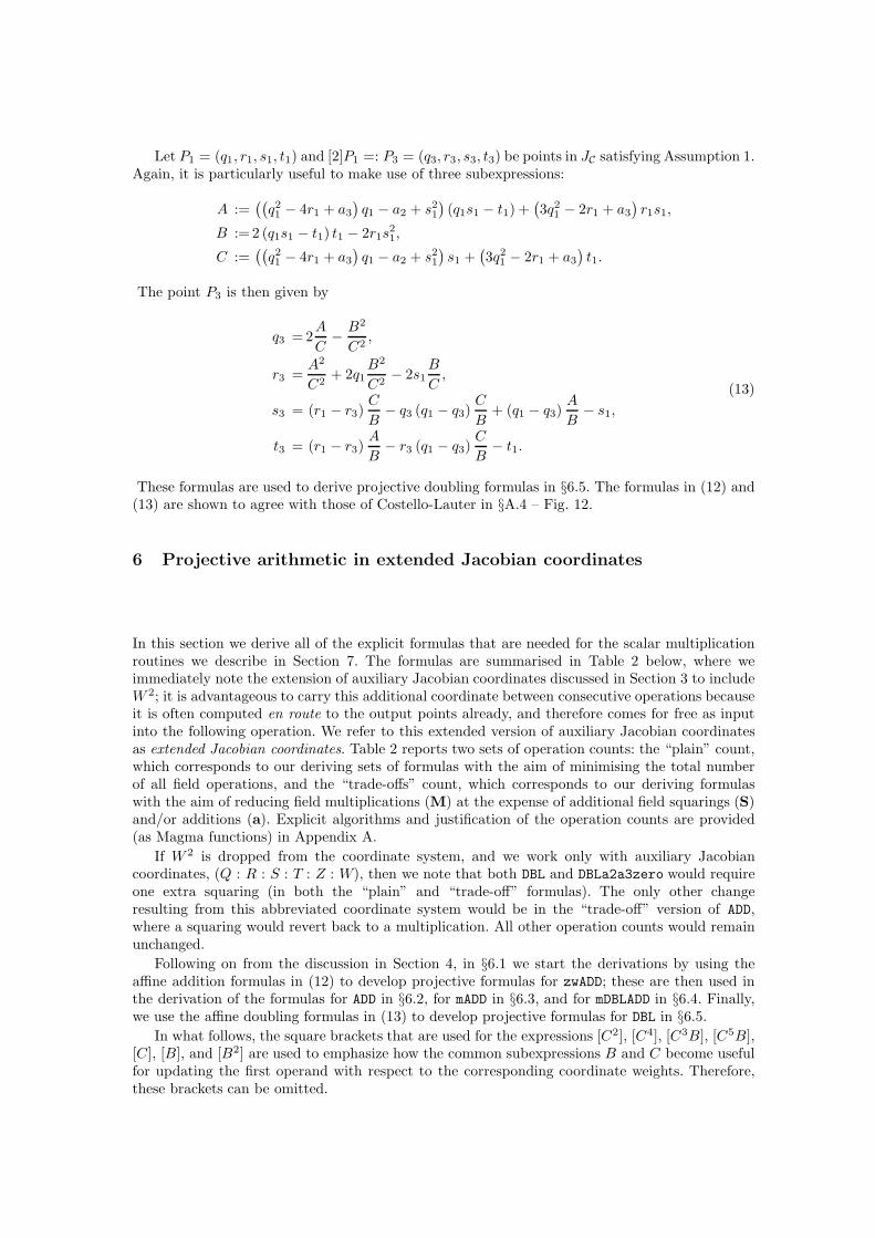
Let P1 = (q1, r1, s1, t1) and [2]P1 =: P3 = (q3, r3, s3, t3) be points in JC satisfying Assumption 1.Again, it is particularly useful to make use of three subexpressions:

A :=((

q21− 4r1 + a3

)

q1 − a2 + s21

)

(q1s1 − t1) +(

3q21− 2r1 + a3

)

r1s1,

B := 2 (q1s1 − t1) t1 − 2r1s2

1,

C :=((

q21 − 4r1 + a3

)

q1 − a2 + s21)

s1 +(

3q21 − 2r1 + a3

)

t1.

The point P3 is then given by

q3 = 2A

C−B2

C2,

r3 =A2

C2+ 2q1

B2

C2− 2s1

B

C,

s3 = (r1 − r3)C

B− q3 (q1 − q3)

C

B+ (q1 − q3)

A

B− s1,

t3 = (r1 − r3)A

B− r3 (q1 − q3)

C

B− t1.

(13)

These formulas are used to derive projective doubling formulas in §6.5. The formulas in (12) and(13) are shown to agree with those of Costello-Lauter in §A.4 – Fig. 12.

6 Projective arithmetic in extended Jacobian coordinates

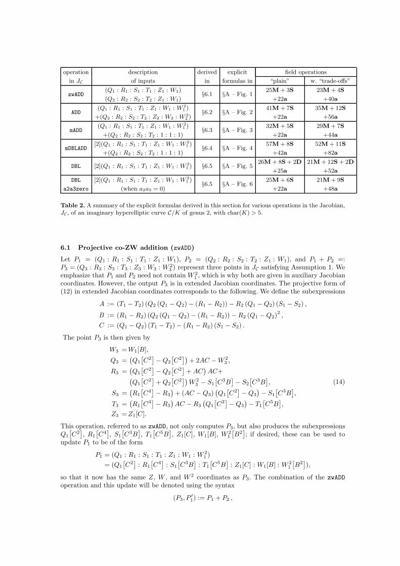
In this section we derive all of the explicit formulas that are needed for the scalar multiplicationroutines we describe in Section 7. The formulas are summarised in Table 2 below, where weimmediately note the extension of auxiliary Jacobian coordinates discussed in Section 3 to includeW 2; it is advantageous to carry this additional coordinate between consecutive operations becauseit is often computed en route to the output points already, and therefore comes for free as inputinto the following operation. We refer to this extended version of auxiliary Jacobian coordinatesas extended Jacobian coordinates. Table 2 reports two sets of operation counts: the “plain” count,which corresponds to our deriving sets of formulas with the aim of minimising the total numberof all field operations, and the “trade-offs” count, which corresponds to our deriving formulaswith the aim of reducing field multiplications (M) at the expense of additional field squarings (S)and/or additions (a). Explicit algorithms and justification of the operation counts are provided(as Magma functions) in Appendix A.

If W 2 is dropped from the coordinate system, and we work only with auxiliary Jacobiancoordinates, (Q : R : S : T : Z : W), then we note that both DBL and DBLa2a3zero would requireone extra squaring (in both the “plain” and “trade-off” formulas). The only other changeresulting from this abbreviated coordinate system would be in the “trade-off” version of ADD,where a squaring would revert back to a multiplication. All other operation counts would remainunchanged.

Following on from the discussion in Section 4, in §6.1 we start the derivations by using theaffine addition formulas in (12) to develop projective formulas for zwADD; these are then used inthe derivation of the formulas for ADD in §6.2, for mADD in §6.3, and for mDBLADD in §6.4. Finally,we use the affine doubling formulas in (13) to develop projective formulas for DBL in §6.5.

In what follows, the square brackets that are used for the expressions [C2], [C4], [C3B], [C5B],[C], [B], and [B2] are used to emphasize how the common subexpressions B and C become usefulfor updating the first operand with respect to the corresponding coordinate weights. Therefore,these brackets can be omitted.

operation description derived explicit field operations

in JC of inputs in formulas in “plain” w. “trade-offs”

zwADD(Q1 : R1 : S1 : T1 : Z1 : W1)

§6.1 §A – Fig. 125M + 3S 23M + 4S

(Q2 : R2 : S2 : T2 : Z1 : W1) +22a +40a

ADD(Q1 : R1 : S1 : T1 : Z1 : W1 : W 2

1 )§6.2 §A – Fig. 2

41M + 7S 35M + 12S

+(Q2 : R2 : S2 : T2 : Z2 : W2 : W 2

2 ) +22a +56a

mADD(Q1 : R1 : S1 : T1 : Z1 : W1 : W 2

1 )§6.3 §A – Fig. 3

32M + 5S 29M + 7S

+(Q2 : R2 : S2 : T2 : 1 : 1 : 1) +22a +44a

mDBLADD[2](Q1 : R1 : S1 : T1 : Z1 : W1 : W 2

1 )§6.4 §A – Fig. 4

57M + 8S 52M + 11S

+(Q2 : R2 : S2 : T2 : 1 : 1 : 1) +42a +82a

DBL [2](Q1 : R1 : S1 : T1 : Z1 : W1 : W 2

1 ) §6.5 §A – Fig. 526M + 8S + 2D 21M + 12S + 2D

+25a +52a

DBL [2](Q1 : R1 : S1 : T1 : Z1 : W1 : W 2

1 )§6.5 §A – Fig. 6

25M + 6S 21M + 9S

a2a3zero (when a2a3 = 0) +22a +48a

Table 2. A summary of the explicit formulas derived in this section for various operations in the Jacobian,JC , of an imaginary hyperelliptic curve C/K of genus 2, with char(K) > 5.

6.1 Projective co-ZW addition (zwADD)

Let P1 = (Q1 : R1 : S1 : T1 : Z1 : W1), P2 = (Q2 : R2 : S2 : T2 : Z1 : W1), and P1 + P2 =:P3 = (Q3 : R3 : S3 : T3 : Z3 : W3 : W 2

3 ) represent three points in JC satisfying Assumption 1. Weemphasize that P1 and P2 need not contain W 2

1, which is why both are given in auxiliary Jacobian

coordinates. However, the output P3 is in extended Jacobian coordinates. The projective form of(12) in extended Jacobian coordinates corresponds to the following. We define the subexpressions

A := (T1 − T2) (Q2 (Q1 −Q2) − (R1 −R2)) −R2 (Q1 −Q2) (S1 − S2) ,

B := (R1 −R2) (Q2 (Q1 −Q2) − (R1 −R2)) −R2 (Q1 −Q2)2 ,

C := (Q1 −Q2) (T1 − T2) − (R1 −R2) (S1 − S2) .

The point P3 is then given by

W3 =W1[B],

Q3 =(

Q1

[

C2]

−Q2

[

C2])

+ 2AC −W 2

3,

R3 =(

Q1

[

C2]

−Q2

[

C2]

+AC)

AC+(

Q1

[

C2]

+Q2

[

C2])

W 2

3− S1

[

C3B]

− S2

[

C3B]

,

S3 =(

R1

[

C4]

−R3

)

+ (AC −Q3)(

Q1

[

C2]

−Q3

)

− S1

[

C3B]

,

T3 =(

R1

[

C4]

−R3

)

AC − R3

(

Q1

[

C2]

−Q3

)

− T1

[

C5B]

,

Z3 =Z1[C].

(14)

This operation, referred to as zwADD, not only computes P3, but also produces the subexpressionsQ1

[

C2]

, R1

[

C4]

, S1

[

C3B]

, T1

[

C5B]

, Z1[C], W1[B], W 2

1

[

B2]

; if desired, these can be used toupdate P1 to be of the form

P1 = (Q1 : R1 : S1 : T1 : Z1 : W1 : W 2

1 )

= (Q1

[

C2]

: R1

[

C4]

: S1

[

C3B]

: T1

[

C5B]

: Z1[C] : W1[B] : W 2

1

[

B2]

),

so that it now has the same Z, W , and W 2 coordinates as P3. The combination of the zwADD

operation and this update will be denoted using the syntax

(P3, P′

1) := P1 + P2 ,

where P ′1

is the updated (but projectively equivalent) version of P1. Explicit formulas for thisoperation are provided in Appendix A – Figure 1; they can be computed in 25M + 3S + 22a, orat the expense of more field additions, in 23M + 4S + 40a using trade-offs.

6.2 Projective addition (ADD)

Rather than producing lengthy formulas for additions, we use a simple construction that exploitszwADD. Let P1 = (Q1 : R1 : S1 : T1 : Z1 : W1 : W 2

1 ), P2 = (Q2 : R2 : S2 : T2 : Z2 : W2 : W 22 ),

and P1 + P2 =: P3 = (Q3 : R3 : S3 : T3 : Z3 : W3 : W 2

3) represent three points in JC satisfying

Assumption 1. We can then cross-multiply to define the points in auxiliary Jacobian coordinates

P ′

1 :=(

Q1

[

Z2

2

]

: R1

[

Z4

2

]

: S1

[

Z3

2W2

]

: T1

[

Z5

2W2

]

: Z1[Z2] : W1[W2])

,

P ′

2 :=(

Q2

[

Z2

1

]

: R2

[

Z4

1

]

: S2

[

Z3

1W1

]

: T2

[

Z5

1W1

]

: Z2[Z1] : W2[W1])

.

Observe that P ′1

= P1 and P ′2

= P2, but that P ′1

and P ′2

now share the same Z and W coordinates.This means that we can use the zwADD operation defined in §6.1 to compute P3 = P1 + P2 as(P3, P

′′1) := P ′

1+ P ′

2. Observe that P ′′

1= P1, and that P ′′

1will share the same Z, W , and W 2

coordinates as P3. We note that this update of P1 into P ′′1

can be useful in the generation oflookup tables [30], but is generally not useful during the main loop. Explicit formulas for thisoperation are provided in Appendix A – Figure 2; they can be computed in 41M + 7S + 22a, orat the expense of more field additions, in 35M + 12S + 56a using trade-offs.

6.3 Projective mixed addition (mADD)

In a similar way, let P1 = (Q1 : R1 : S1 : T1 : Z1 : W1 : W 2

1), P2 = (Q2 : R2 : S2 : T2 : 1 : 1 : 1),

and P1 + P2 =: P3 = (Q3 : R3 : S3 : T3 : Z3 : W3 : W 2

3) represent three points in JC satisfying

Assumption 1. This time we only need to update P2 into P ′2, which is performed in auxiliary

Jacobian coordinates as

P ′

2 :=(

Q2

[

Z2

1

]

: R2

[

Z4

1

]

: S2

[

Z3

1W1

]

: T2

[

Z5

1W1

]

: [Z1] : [W1])

,

where we observe that P1 and P ′2

now have the same Z and W coordinates. Subsequently, usingthe zwADD operation from §6.1 allows P3 = P1+P2 to be computed by (P3, P

′1) := P1+P ′

2. Explicitformulas are provided in Appendix A – Figure 3; they can be computed in 32M+ 5S+ 22a, or atthe expense of more field additions, in 29M + 7S + 44a using trade-offs.

6.4 Projective mixed doubling-and-addition (mDBLADD)

Let P1 = (Q1 : R1 : S1 : T1 : Z1 : W1 : W 2

1 ), P2 = (Q2 : R2 : S2 : T2 : 1 : 1 : 1), and [2]P1 + P2 =:P3 = (Q3 : R3 : S3 : T3 : Z3 : W3 : W 2

3), represent three points in JC satisfying Assumption 1. To

compute [2]P1 +P2, we schedule the higher level operations in the form (P1 +P2)+P1 (see [15] and[30] for the same high level scheduling). This means that mDBLADD can be computed using an mADD

operation before a zwADD operation. (Subsequently, we must also assume that P1, the intermediatepoint P1+P2, and the output point [2]P1+P2 =: P3 = (Q3 : R3 : S3 : T3 : Z3 : W3 : W 2

3 ) representthree points in JC satisfying Assumption 1.) Following §6.2 and §6.3, this can be computed in57M+8S+42a, or at the expense of more additions, in 52M+11S+60a using trade-offs. Explicitformulas for the mDBLADD operation are provided in Appendix A – Figure 4.

6.5 Projective doubling (DBL)

Let P1 = (Q1 : R1 : S1 : T1 : Z1 : W1 : W 2

1) and [2]P1 =: P3 = (Q3 : R3 : S3 : T3 : Z3 : W3 : W 2

3)

represent two points in JC satisfying Assumption 1. The projective form of (13) in extended

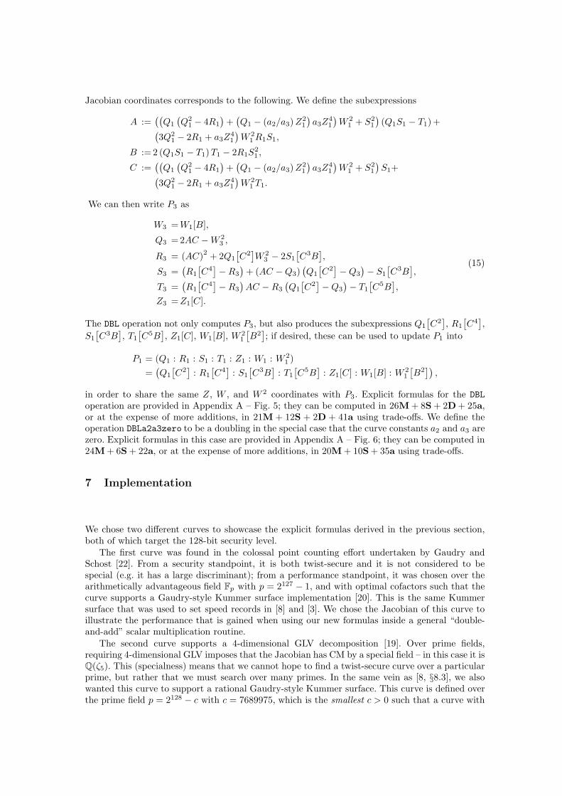
Jacobian coordinates corresponds to the following. We define the subexpressions

A :=((

Q1

(

Q2

1 − 4R1

)

+(

Q1 − (a2/a3)Z2

1

)

a3Z4

1

)

W 2

1 + S2

1

)

(Q1S1 − T1)+(

3Q2

1− 2R1 + a3Z

4

1

)

W 2

1R1S1,

B := 2 (Q1S1 − T1)T1 − 2R1S2

1,

C :=((

Q1

(

Q2

1− 4R1

)

+(

Q1 − (a2/a3)Z2

1

)

a3Z4

1

)

W 2

1+ S2

1

)

S1+(

3Q2

1 − 2R1 + a3Z4

1

)

W 2

1 T1.

We can then write P3 as

W3 =W1[B],

Q3 =2AC −W 2

3,

R3 = (AC)2 + 2Q1

[

C2]

W 2

3− 2S1

[

C3B]

,

S3 =(

R1

[

C4]

−R3

)

+ (AC −Q3)(

Q1

[

C2]

−Q3

)

− S1

[

C3B]

,

T3 =(

R1

[

C4]

−R3

)

AC − R3

(

Q1

[

C2]

−Q3

)

− T1

[

C5B]

,

Z3 =Z1[C].

(15)

The DBL operation not only computes P3, but also produces the subexpressions Q1

[

C2]

, R1

[

C4]

,

S1

[

C3B]

, T1

[

C5B]

, Z1[C], W1[B], W 2

1

[

B2]

; if desired, these can be used to update P1 into

P1 = (Q1 : R1 : S1 : T1 : Z1 : W1 : W 2

1)

=(

Q1

[

C2]

: R1

[

C4]

: S1

[

C3B]

: T1

[

C5B]

: Z1[C] : W1[B] : W 2

1

[

B2])

,

in order to share the same Z, W , and W 2 coordinates with P3. Explicit formulas for the DBL

operation are provided in Appendix A – Fig. 5; they can be computed in 26M + 8S + 2D + 25a,or at the expense of more additions, in 21M + 12S + 2D + 41a using trade-offs. We define theoperation DBLa2a3zero to be a doubling in the special case that the curve constants a2 and a3 arezero. Explicit formulas in this case are provided in Appendix A – Fig. 6; they can be computed in24M + 6S + 22a, or at the expense of more additions, in 20M + 10S + 35a using trade-offs.

7 Implementation

We chose two different curves to showcase the explicit formulas derived in the previous section,both of which target the 128-bit security level.

The first curve was found in the colossal point counting effort undertaken by Gaudry andSchost [22]. From a security standpoint, it is both twist-secure and it is not considered to bespecial (e.g. it has a large discriminant); from a performance standpoint, it was chosen over thearithmetically advantageous field Fp with p = 2127 − 1, and with optimal cofactors such that thecurve supports a Gaudry-style Kummer surface implementation [20]. This is the same Kummersurface that was used to set speed records in [8] and [3]. We chose the Jacobian of this curve toillustrate the performance that is gained when using our new formulas inside a general “double-and-add” scalar multiplication routine.

The second curve supports a 4-dimensional GLV decomposition [19]. Over prime fields,requiring 4-dimensional GLV imposes that the Jacobian has CM by a special field – in this case it isQ(ζ5). This (specialness) means that we cannot hope to find a twist-secure curve over a particularprime, but rather that we must search over many primes. In the same vein as [8, §8.3], we alsowanted this curve to support a rational Gaudry-style Kummer surface. This curve is defined overthe prime field p = 2128 − c with c = 7689975, which is the smallest c > 0 such that a curve with

CM by Q(ζ5) over Fp is twist-secure with optimal cofactors6. This curve was chosen to exhibit theperformance that is gained when using our new formulas inside a GLV-style multiexponentation;in particular, each step of the multiexponentation requires only an mDBLADD operation, and this iswhere our explicit formulas offer the largest relative speedup over the previous ones.

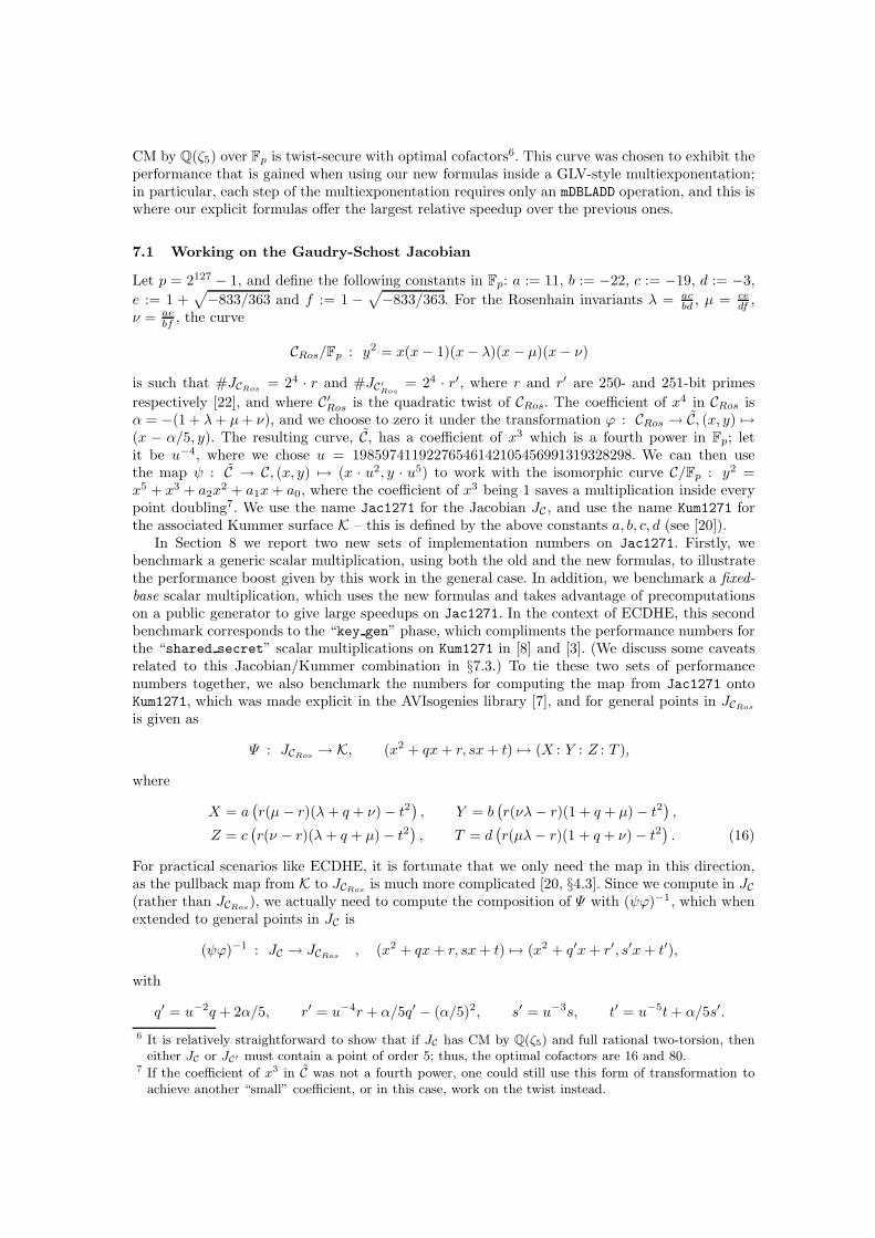
7.1 Working on the Gaudry-Schost Jacobian

Let p = 2127 − 1, and define the following constants in Fp: a := 11, b := −22, c := −19, d := −3,

e := 1 +√

−833/363 and f := 1 −√

−833/363. For the Rosenhain invariants λ = acbd

, µ = cedf

,ν = ae

bf, the curve

CRos/Fp : y2 = x(x − 1)(x− λ)(x − µ)(x− ν)

is such that #JCRos= 24 · r and #JC′

Ros= 24 · r′, where r and r′ are 250- and 251-bit primes

respectively [22], and where C′

Ros is the quadratic twist of CRos. The coefficient of x4 in CRos isα = −(1 + λ+ µ+ ν), and we choose to zero it under the transformation ϕ : CRos → C, (x, y) 7→(x − α/5, y). The resulting curve, C, has a coefficient of x3 which is a fourth power in Fp; letit be u−4, where we chose u = 19859741192276546142105456991319328298. We can then usethe map ψ : C → C, (x, y) 7→ (x · u2, y · u5) to work with the isomorphic curve C/Fp : y2 =x5 + x3 + a2x

2 + a1x+ a0, where the coefficient of x3 being 1 saves a multiplication inside everypoint doubling7. We use the name Jac1271 for the Jacobian JC , and use the name Kum1271 forthe associated Kummer surface K – this is defined by the above constants a, b, c, d (see [20]).

In Section 8 we report two new sets of implementation numbers on Jac1271. Firstly, webenchmark a generic scalar multiplication, using both the old and the new formulas, to illustratethe performance boost given by this work in the general case. In addition, we benchmark a fixed-base scalar multiplication, which uses the new formulas and takes advantage of precomputationson a public generator to give large speedups on Jac1271. In the context of ECDHE, this secondbenchmark corresponds to the “key gen” phase, which compliments the performance numbers forthe “shared secret” scalar multiplications on Kum1271 in [8] and [3]. (We discuss some caveatsrelated to this Jacobian/Kummer combination in §7.3.) To tie these two sets of performancenumbers together, we also benchmark the numbers for computing the map from Jac1271 ontoKum1271, which was made explicit in the AVIsogenies library [7], and for general points in JCRos

is given as

Ψ : JCRos→ K, (x2 + qx+ r, sx+ t) 7→ (X : Y : Z : T ),

where

X = a(

r(µ − r)(λ + q + ν) − t2)

, Y = b(

r(νλ − r)(1 + q + µ) − t2)

,

Z = c(

r(ν − r)(λ + q + µ) − t2)

, T = d(

r(µλ − r)(1 + q + ν) − t2)

. (16)

For practical scenarios like ECDHE, it is fortunate that we only need the map in this direction,as the pullback map from K to JCRos

is much more complicated [20, §4.3]. Since we compute in JC(rather than JCRos

), we actually need to compute the composition of Ψ with (ψϕ)−1, which whenextended to general points in JC is

(ψϕ)−1 : JC → JCRos, (x2 + qx+ r, sx+ t) 7→ (x2 + q′x+ r′, s′x+ t′),

with

q′ = u−2q + 2α/5, r′ = u−4r + α/5q′ − (α/5)2, s′ = u−3s, t′ = u−5t+ α/5s′.

6 It is relatively straightforward to show that if JC has CM by Q(ζ5) and full rational two-torsion, theneither JC or JC′ must contain a point of order 5; thus, the optimal cofactors are 16 and 80.

7 If the coefficient of x3 in C was not a fourth power, one could still use this form of transformation toachieve another “small” coefficient, or in this case, work on the twist instead.

Assuming that the input point in JC is in extended Jacobian coordinates, the operation count forthe full map Ψ ′ = Ψ(ψϕ)−1 from JC to K is 1I+31M+2S+19a (see Figure 10 in Appendix A.2);we benchmark it alongside the scalar multiplications in Section 8.

To draw a fair comparison against prior works, we inserted our formulas into the softwaremade publicly available by Bos et al. [8], which itself employed the previous best formulas. (Wetweaked both sets of formulas for Jac1271 to take advantage of the constant a3 = 1.) Thissoftware computes the scalar multiplications on Jac1271 using a left-to-right signed sliding windowrecoding [1] with a window size of w = 5, where the lookup table consists of 8 points and isconstructed exactly as in [30, §4]. The timings are presented in Section 8.

7.2 Working on the Jacobian of a GLV curve

Let p = 2128 − 7689975 and define C/Fp : y2 = x5 + 710. The Jacobian groups JC and JC′ havecardinalities #JC = 24 · 5 · r and #JC′ = 24 · r′, where

r =(

2252 + 375576928331233691782146792677798267213584131651764404159)

/5 and

r′ = 2252 − 375576928331887882475846226038533397089218679777223482485

are both prime.The implementation of a 4-dimensional GLV scalar multiplication in JC follows that which is

described in [8, §6]; again, we wrapped their GLV software around both their old and our newformulas for a fair comparison – we note that both instances were made to use the above curve,which we refer to as GLV128c.

Practically speaking, it does not make as much sense to benchmark GLV128c in the sameECDHE style as we discussed for Jac1271 and Kum1271. If there is enough storage to exploita long-term public generator P , then the presence of endomorphisms is essentially redundantin the key gen phase, since multiples of P can then be precomputed offline without usingan endomorphism. On the shared secret side, where variable-base scalar multiplications areperformed on fresh inputs, our implementations show that a 4-dimensional decomposition onGLV128c is still slightly slower than a Kummer surface scalar multiplication, so in the case ofECDHE, it is likely to be faster on both sides to stick with the combination of Jac1271 andKum1271. Nevertheless, there could be scenarios where it makes sense to use the endomorphism onGLV128c (e.g. for a signature verification), and still make use of the maps between the full Jacobiangroup and the associated Kummer surface. In this case, the map in (16) and the pullback mapin [20, §4.3] can be exploited analogously to the case of Jac1271, keeping in mind that the mapswould pass through the Jacobian of the Rosenhain form of C.

Timings for a 4-dimensional GLV variable-base scalar multiplication on GLV128c using boththe old and the new explicit formulas are given in Section 8.

We note that in all scalar multiplication routines, i.e. in both fixed- and variable-base scalarmultiplications on Jac1271 and in 4-dimensional multiexponentiations on GLV128c, we alwaysfound it advantageous to convert the lookup table elements from extended Jacobian coordinatesto affine coordinates using Montgomery’s simultaneous inversion method [34]. This “decision” isgenerally made easier in genus 2, where the difference between mixed additions and full additions isgreater, and the relative cost of a field inversion (compared to the rest of the scalar multiplicationroutine) is much less than it is in the elliptic curve case. Finally, we note that the single conversionof the output point from Jacobian to affine coordinates comes at a cost of 1I + 10M + 1S (seeFigure 9 in Appendix A.2).

7.3 A disclaimer: the difficulties facing constant-time, exception-free scalarmultiplications in JC

We must point out that none of the scalar multiplications on Jac1271 or GLV128c that we reportin this paper run in constant time, and that the difficulties of achieving such a routine in genus 2

Jacobians is closely related to Assumption 1. We note that these are not the same implementation-level difficulties pointed out in [3, §1.2]; indeed, while the Kummer surface implementationsreported in [3] and [8] run in constant time, a truly constant-time genus 2 implementation thatdoes not use the Kummer surface is yet to be documented in the literature.

More specifically, there are scalar recoding algorithms (cf. [24, 16]) that seemingly make itpossible to implement the Jac1271 or GLV128c routines such that scalar multiplications on randominputs will run in constant time with probability exponentially close to 1. However, in order toguard against active adversaries and to be considered truly constant-time, the routines should beguaranteed to execute identically and run correctly for all combinations of integer scalars andinput points; this means the explicit formulas must be able to handle input combinations in JCthat are not “general” in the sense of Assumption 1. Although explicit formulas can be developedfor each of these special cases, their culmination into an efficient and truly constant-time scalarmultiplication algorithm remains an important open problem.

8 Results

In this section we present the timings of the routines described in the previous section. All of thebenchmarks were performed on an Intel Core i7-3770M (Ivy Bridge) processor at 3.4 GHz withhyperthreading turned off and over-clocking (“turbo-boost”) disabled, and all-but-one of the coresswitched off in BIOS. The implementations were compiled with gcc 4.6.3 with the -O2 flag set andtested on a 64-bit Linux environment. Cycles were obtained using the SUPERCOP [6] toolkit andthen rounded to the nearest 1,000 cycles.

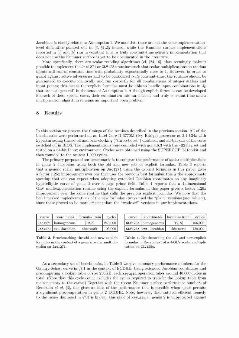
The primary purpose of our benchmarks is to compare the performance of scalar multiplicationsin genus 2 Jacobians using both the old and new sets of explicit formulas. Table 3 reportsthat a generic scalar multiplication on Jac1271 using the explicit formulas in this paper givesa factor 1.25x improvement over one that uses the previous best formulas; this is the approximatespeedup that one can expect when adopting extended Jacobian coordinates on any imaginaryhyperelliptic curve of genus 2 over a large prime field. Table 4 reports that a 4-dimensionalGLV multiexponentiation routine using the explicit formulas in this paper gives a factor 1.29ximprovement over the same routine that calls the previous explicit formulas. We note that thebenchmarked implementations of the new formulas always used the “plain” versions (see Table 2),since these proved to be more efficient than the “trade-off” versions in our implementations.

curve coordinates formulas from cycles

Jac1271 homogeneous [12, 8] 243,000

Jac1271 ext. Jacobian this work 195,000

Table 3. Benchmarking the old and new explicitformulas in the context of a generic scalar multipli-cation on Jac1271.

curve coordinates formulas from cycles

GLV128c homogeneous [12, 8] 166,000

GLV128c ext. Jacobian this work 129,000

Table 4. Benchmarking the old and new explicitformulas in the context of a 4-GLV scalar multipli-cation on GLV128c.

As a secondary set of benchmarks, in Table 5 we give summary performance numbers for theGaudry-Schost curve in §7.1 in the context of ECDHE. Using extended Jacobian coordinates andprecomputing a lookup table of size 256KB, each key gen operation takes around 40,000 cycles intotal. (Note that this cycle count excludes the cycles required to transfer the lookup table frommain memory to the cache.) Together with the recent Kummer surface performance numbers ofBernstein et al. [3], this gives an idea of the performance that is possible when space permitsa significant precomputation in genus 2 ECDHE. Note, however, that until an efficient remedyto the issues discussed in §7.3 is known, this style of key gen in genus 2 is unprotected against

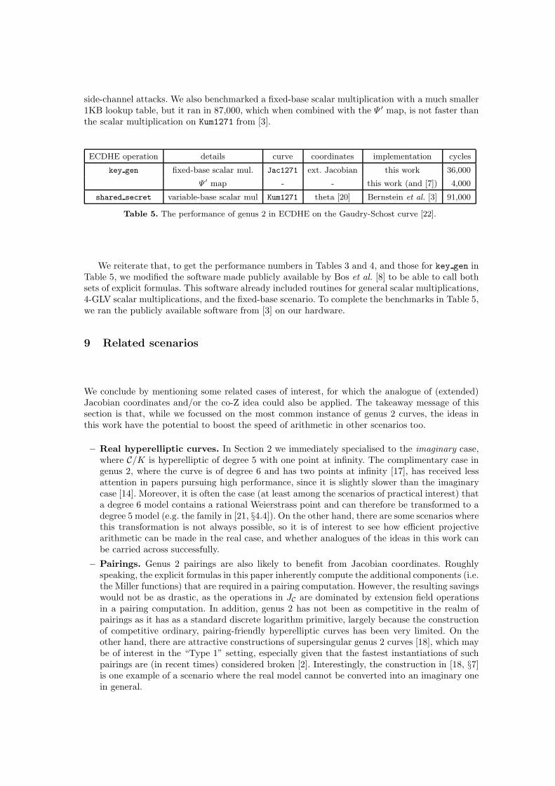
side-channel attacks. We also benchmarked a fixed-base scalar multiplication with a much smaller1KB lookup table, but it ran in 87,000, which when combined with the Ψ ′ map, is not faster thanthe scalar multiplication on Kum1271 from [3].

ECDHE operation details curve coordinates implementation cycles

key gen fixed-base scalar mul. Jac1271 ext. Jacobian this work 36,000

Ψ ′ map - - this work (and [7]) 4,000

shared secret variable-base scalar mul Kum1271 theta [20] Bernstein et al. [3] 91,000

Table 5. The performance of genus 2 in ECDHE on the Gaudry-Schost curve [22].

We reiterate that, to get the performance numbers in Tables 3 and 4, and those for key gen inTable 5, we modified the software made publicly available by Bos et al. [8] to be able to call bothsets of explicit formulas. This software already included routines for general scalar multiplications,4-GLV scalar multiplications, and the fixed-base scenario. To complete the benchmarks in Table 5,we ran the publicly available software from [3] on our hardware.

9 Related scenarios

We conclude by mentioning some related cases of interest, for which the analogue of (extended)Jacobian coordinates and/or the co-Z idea could also be applied. The takeaway message of thissection is that, while we focussed on the most common instance of genus 2 curves, the ideas inthis work have the potential to boost the speed of arithmetic in other scenarios too.

– Real hyperelliptic curves. In Section 2 we immediately specialised to the imaginary case,where C/K is hyperelliptic of degree 5 with one point at infinity. The complimentary case ingenus 2, where the curve is of degree 6 and has two points at infinity [17], has received lessattention in papers pursuing high performance, since it is slightly slower than the imaginarycase [14]. Moreover, it is often the case (at least among the scenarios of practical interest) thata degree 6 model contains a rational Weierstrass point and can therefore be transformed to adegree 5 model (e.g. the family in [21, §4.4]). On the other hand, there are some scenarios wherethis transformation is not always possible, so it is of interest to see how efficient projectivearithmetic can be made in the real case, and whether analogues of the ideas in this work canbe carried across successfully.

– Pairings. Genus 2 pairings are also likely to benefit from Jacobian coordinates. Roughlyspeaking, the explicit formulas in this paper inherently compute the additional components (i.e.the Miller functions) that are required in a pairing computation. However, the resulting savingswould not be as drastic, as the operations in JC are dominated by extension field operationsin a pairing computation. In addition, genus 2 has not been as competitive in the realm ofpairings as it has as a standard discrete logarithm primitive, largely because the constructionof competitive ordinary, pairing-friendly hyperelliptic curves has been very limited. On theother hand, there are attractive constructions of supersingular genus 2 curves [18], which maybe of interest in the “Type 1” setting, especially given that the fastest instantiations of suchpairings are (in recent times) considered broken [2]. Interestingly, the construction in [18, §7]is one example of a scenario where the real model cannot be converted into an imaginary onein general.

– Low characteristic / higher genus. The specialisation of Jacobian coordinates to lowcharacteristic genus 2 curves and the extension to higher genus imaginary hyperelliptic curvesfollows analogously. However, the motivation in both directions is nowadays stunted by theirrespective security concerns. Nevertheless, it could be worthwhile to see how much faster thearithmetic in these cases can become when using Jacobian coordinates.

– The RM families. We benchmarked the new explicit formulas in two scenarios; on a non-special “generic” curve, and on a curve with very special CM that subsequently comes equippedwith an endomorphism. A third option comes from the families with explicit RM in [21],which perhaps achieves the best of both worlds in genus 2: they are constructed to have anendomorphism, but are much more general than the CM curve we used. This generality dispelsany security concerns associated with special curves, and moreover allows them to be foundover a fixed prime field. Thus, at the 128-bit security level, one could find such a curve overp = 2127−1 that facilitates both 2-dimensional GLV decomposition on its Jacobian and whichsupports a (twist-secure) Kummer surface. It would then be very interesting to benchmarkthe new explicit formulas on one of these families, where the GLV routine would again makea higher relative frequency of calls to the fast mDBLADD routine.

Acknowledgements. We thank Joppe Bos, Michael Naehrig, Benjamin Smith, and OsmanbeyUzunkol for their useful comments on an early draft of this work.

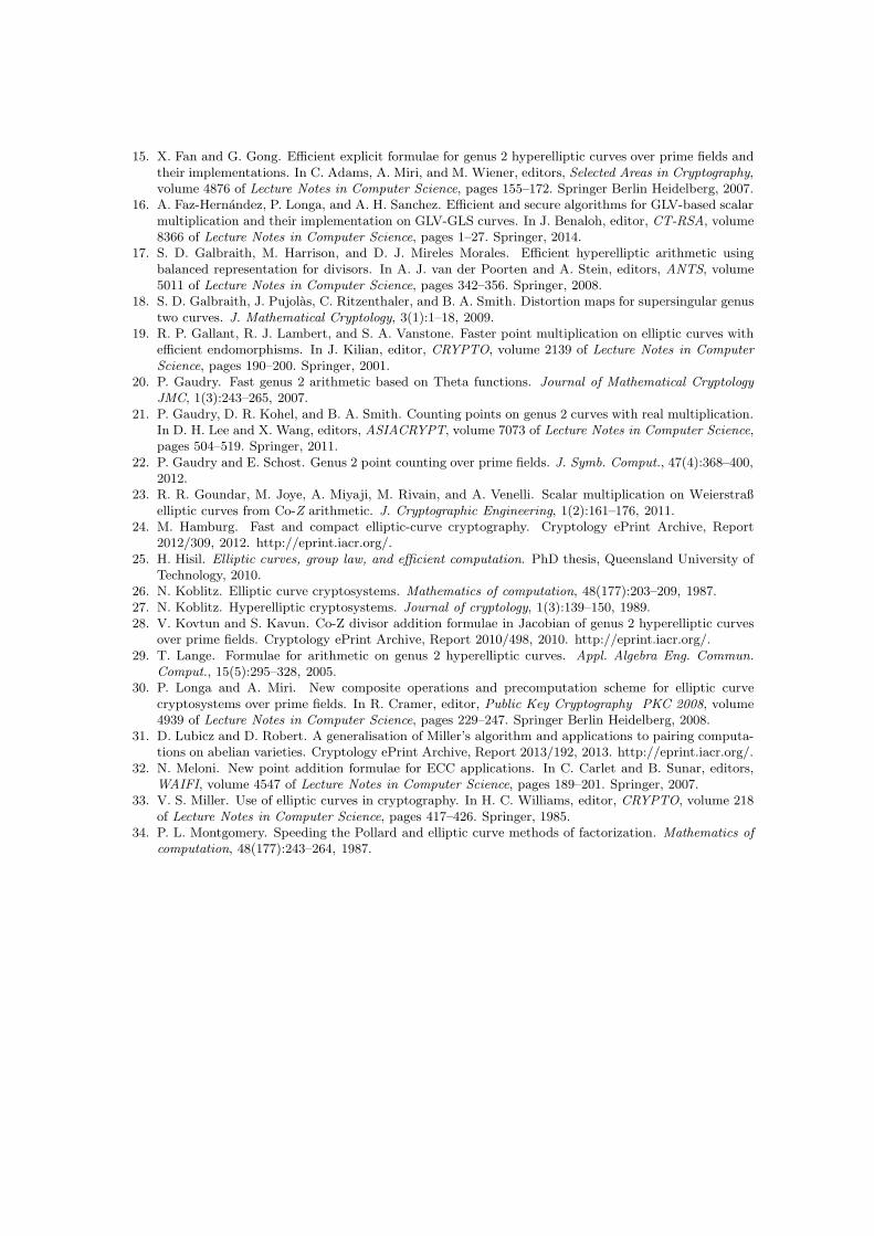
References

1. R. M. Avanzi. A note on the signed sliding window integer recoding and a left-to-right analogue.In H. Handschuh and M. A. Hasan, editors, Selected Areas in Cryptography, volume 3357 of LectureNotes in Computer Science, pages 130–143. Springer, 2004.

2. R. Barbulescu, P. Gaudry, A. Joux, and E. Thome. A heuristic quasi-polynomial algorithm fordiscrete logarithm in finite fields of small characteristic. In P. Q. Nguyen and E. Oswald, editors,EUROCRYPT, volume 8441 of Lecture Notes in Computer Science, pages 1–16. Springer, 2014.

3. D. J. Bernstein, C. Chuengsatiansup, T. Lange, and P. Schwabe. Kummer strikes back: new DH speedrecords. IACR Cryptology ePrint Archive, 2014:134, 2014.

4. D. J. Bernstein and T. Lange. Faster addition and doubling on elliptic curves. In ASIACRYPT 2007,volume 4833 of LNCS, pages 29–50. Springer, 2007.

5. D. J. Bernstein and T. Lange. Explicit-formulas database, accessed 2 Jan, 2014.http://www.hyperelliptic.org/EFD/.

6. D. J. Bernstein and T. Lange. eBACS: ECRYPT Benchmarking of Cryptographic Systems, accessed28 September, 2013. http://bench.cr.yp.to.

7. G. Bisson, R. Cosset, and D. Robert. AVIsogenies – a library for computing isogenies between abelianvarieties, November 2012. URL: http://avisogenies.gforge.inria.fr.

8. J. W. Bos, C. Costello, H. Hisil, and K. Lauter. Fast cryptography in genus 2. In T. Johanssonand P. Q. Nguyen, editors, EUROCRYPT, volume 7881 of Lecture Notes in Computer Science, pages194–210. Springer, 2013, full version available at: http://eprint.iacr.org/2012/670.

9. W. Bosma, J. Cannon, and C. Playoust. The Magma algebra system. I. The user language. J. SymbolicComput., 24(3-4):235–265, 1997. Computational algebra and number theory (London, 1993).

10. E. Brier and M. Joye. Weierstraß elliptic curves and side-channel attacks. In Public Key Cryptography,pages 335–345. Springer, 2002.

11. D. V. Chudnovsky and G. V. Chudnovsky. Sequences of numbers generated by addition in formalgroups and new primality and factorization tests. Advances in Applied Mathematics, 7(4):385–434,1986.

12. C. Costello and K. Lauter. Group law computations on Jacobians of hyperelliptic curves. In A. Miriand S. Vaudenay, editors, Selected Areas in Cryptography, volume 7118 of Lecture Notes in ComputerScience, pages 92–117. Springer, 2011.

13. O. Diao and M. Joye. Unified addition formulæ for hyperelliptic curve cryptosystems. In 3rd Workshopon Mathematical Cryptology (WMC 2012) and 3rd International Conference on Symbolic Computationand Cryptography (SCC 2012), pages 45–50, 2012.

14. S. Erickson, T. Ho, and S. Zemedkun. Explicit projective formulas for real hyperelliptic curves ofgenus 2. Personal Communication, May 2014.

15. X. Fan and G. Gong. Efficient explicit formulae for genus 2 hyperelliptic curves over prime fields andtheir implementations. In C. Adams, A. Miri, and M. Wiener, editors, Selected Areas in Cryptography,volume 4876 of Lecture Notes in Computer Science, pages 155–172. Springer Berlin Heidelberg, 2007.

16. A. Faz-Hernandez, P. Longa, and A. H. Sanchez. Efficient and secure algorithms for GLV-based scalarmultiplication and their implementation on GLV-GLS curves. In J. Benaloh, editor, CT-RSA, volume8366 of Lecture Notes in Computer Science, pages 1–27. Springer, 2014.

17. S. D. Galbraith, M. Harrison, and D. J. Mireles Morales. Efficient hyperelliptic arithmetic usingbalanced representation for divisors. In A. J. van der Poorten and A. Stein, editors, ANTS, volume5011 of Lecture Notes in Computer Science, pages 342–356. Springer, 2008.

18. S. D. Galbraith, J. Pujolas, C. Ritzenthaler, and B. A. Smith. Distortion maps for supersingular genustwo curves. J. Mathematical Cryptology, 3(1):1–18, 2009.

19. R. P. Gallant, R. J. Lambert, and S. A. Vanstone. Faster point multiplication on elliptic curves withefficient endomorphisms. In J. Kilian, editor, CRYPTO, volume 2139 of Lecture Notes in ComputerScience, pages 190–200. Springer, 2001.

20. P. Gaudry. Fast genus 2 arithmetic based on Theta functions. Journal of Mathematical CryptologyJMC, 1(3):243–265, 2007.

21. P. Gaudry, D. R. Kohel, and B. A. Smith. Counting points on genus 2 curves with real multiplication.In D. H. Lee and X. Wang, editors, ASIACRYPT, volume 7073 of Lecture Notes in Computer Science,pages 504–519. Springer, 2011.

22. P. Gaudry and E. Schost. Genus 2 point counting over prime fields. J. Symb. Comput., 47(4):368–400,2012.

23. R. R. Goundar, M. Joye, A. Miyaji, M. Rivain, and A. Venelli. Scalar multiplication on Weierstraßelliptic curves from Co-Z arithmetic. J. Cryptographic Engineering, 1(2):161–176, 2011.

24. M. Hamburg. Fast and compact elliptic-curve cryptography. Cryptology ePrint Archive, Report2012/309, 2012. http://eprint.iacr.org/.

25. H. Hisil. Elliptic curves, group law, and efficient computation. PhD thesis, Queensland University ofTechnology, 2010.

26. N. Koblitz. Elliptic curve cryptosystems. Mathematics of computation, 48(177):203–209, 1987.27. N. Koblitz. Hyperelliptic cryptosystems. Journal of cryptology, 1(3):139–150, 1989.28. V. Kovtun and S. Kavun. Co-Z divisor addition formulae in Jacobian of genus 2 hyperelliptic curves

over prime fields. Cryptology ePrint Archive, Report 2010/498, 2010. http://eprint.iacr.org/.29. T. Lange. Formulae for arithmetic on genus 2 hyperelliptic curves. Appl. Algebra Eng. Commun.

Comput., 15(5):295–328, 2005.30. P. Longa and A. Miri. New composite operations and precomputation scheme for elliptic curve

cryptosystems over prime fields. In R. Cramer, editor, Public Key Cryptography PKC 2008, volume4939 of Lecture Notes in Computer Science, pages 229–247. Springer Berlin Heidelberg, 2008.

31. D. Lubicz and D. Robert. A generalisation of Miller’s algorithm and applications to pairing computa-tions on abelian varieties. Cryptology ePrint Archive, Report 2013/192, 2013. http://eprint.iacr.org/.

32. N. Meloni. New point addition formulae for ECC applications. In C. Carlet and B. Sunar, editors,WAIFI, volume 4547 of Lecture Notes in Computer Science, pages 189–201. Springer, 2007.

33. V. S. Miller. Use of elliptic curves in cryptography. In H. C. Williams, editor, CRYPTO, volume 218of Lecture Notes in Computer Science, pages 417–426. Springer, 1985.

34. P. L. Montgomery. Speeding the Pollard and elliptic curve methods of factorization. Mathematics ofcomputation, 48(177):243–264, 1987.

A Appendix

Section A.1 of this appendix provides justifications for all claimed operation counts with explicitalgorithms. Section A.2 provides explicit algorithms for the coordinate conversions and mapsused in this work. Section A.3 proposes new unified addition formulas/algorithms and theircorresponding operation counts. Finally, Section A.4 provides Magma [9] scripts to show howthe proposed formulas compare to the existing formulas in the literature.

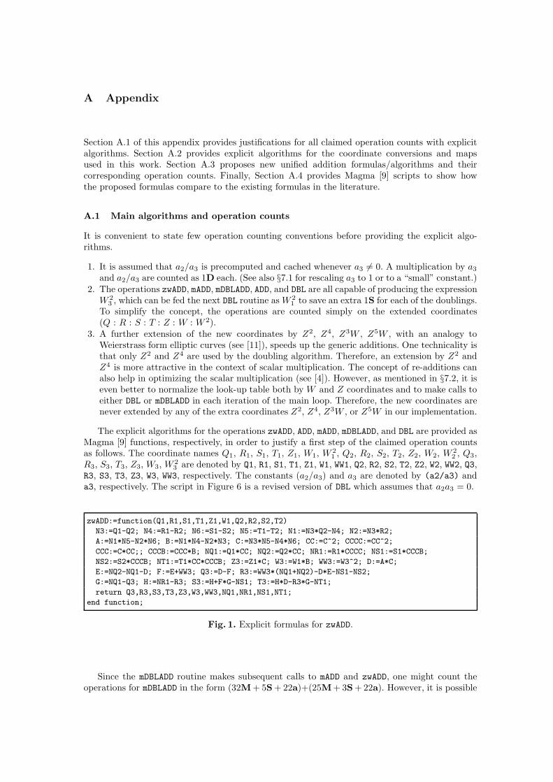
A.1 Main algorithms and operation counts

It is convenient to state few operation counting conventions before providing the explicit algo-rithms.

1. It is assumed that a2/a3 is precomputed and cached whenever a3 6= 0. A multiplication by a3

and a2/a3 are counted as 1D each. (See also §7.1 for rescaling a3 to 1 or to a “small” constant.)2. The operations zwADD, mADD, mDBLADD, ADD, and DBL are all capable of producing the expressionW 2

3 , which can be fed the next DBL routine as W 2

1 to save an extra 1S for each of the doublings.To simplify the concept, the operations are counted simply on the extended coordinates(Q : R : S : T : Z : W : W 2).

3. A further extension of the new coordinates by Z2, Z4, Z3W , Z5W , with an analogy toWeierstrass form elliptic curves (see [11]), speeds up the generic additions. One technicality isthat only Z2 and Z4 are used by the doubling algorithm. Therefore, an extension by Z2 andZ4 is more attractive in the context of scalar multiplication. The concept of re-additions canalso help in optimizing the scalar multiplication (see [4]). However, as mentioned in §7.2, it iseven better to normalize the look-up table both by W and Z coordinates and to make calls toeither DBL or mDBLADD in each iteration of the main loop. Therefore, the new coordinates arenever extended by any of the extra coordinates Z2, Z4, Z3W , or Z5W in our implementation.

The explicit algorithms for the operations zwADD, ADD, mADD, mDBLADD, and DBL are provided asMagma [9] functions, respectively, in order to justify a first step of the claimed operation countsas follows. The coordinate names Q1, R1, S1, T1, Z1, W1, W

2

1, Q2, R2, S2, T2, Z2, W2, W

2

2, Q3,

R3, S3, T3, Z3, W3, W2

3are denoted by Q1, R1, S1, T1, Z1, W1, WW1, Q2, R2, S2, T2, Z2, W2, WW2, Q3,

R3, S3, T3, Z3, W3, WW3, respectively. The constants (a2/a3) and a3 are denoted by (a2/a3) anda3, respectively. The script in Figure 6 is a revised version of DBL which assumes that a2a3 = 0.

zwADD:=function(Q1,R1,S1,T1,Z1,W1,Q2,R2,S2,T2)

N3:=Q1-Q2; N4:=R1-R2; N6:=S1-S2; N5:=T1-T2; N1:=N3*Q2-N4; N2:=N3*R2;

A:=N1*N5-N2*N6; B:=N1*N4-N2*N3; C:=N3*N5-N4*N6; CC:=C^2; CCCC:=CC^2;

CCC:=C*CC;; CCCB:=CCC*B; NQ1:=Q1*CC; NQ2:=Q2*CC; NR1:=R1*CCCC; NS1:=S1*CCCB;

NS2:=S2*CCCB; NT1:=T1*CC*CCCB; Z3:=Z1*C; W3:=W1*B; WW3:=W3^2; D:=A*C;

E:=NQ2-NQ1-D; F:=E+WW3; Q3:=D-F; R3:=WW3*(NQ1+NQ2)-D*E-NS1-NS2;

G:=NQ1-Q3; H:=NR1-R3; S3:=H+F*G-NS1; T3:=H*D-R3*G-NT1;

return Q3,R3,S3,T3,Z3,W3,WW3,NQ1,NR1,NS1,NT1;

end function;

Fig. 1. Explicit formulas for zwADD.

Since the mDBLADD routine makes subsequent calls to mADD and zwADD, one might count theoperations for mDBLADD in the form (32M + 5S + 22a)+(25M+ 3S + 22a). However, it is possible

ADD:=function(Q1,R1,S1,T1,Z1,W1,WW1,Q2,R2,S2,T2,Z2,W2,WW2)

ZZ1:=Z1^2; ZZZZ1:=ZZ1^2; ZZZ1:=ZZ1*Z1;; ZZZW1:=ZZZ1*W1; NW1:=W1*W2;;;

ZZ2:=Z2^2; ZZZZ2:=ZZ2^2; ZZZ2:=ZZ2*Z2;; ZZZW2:=ZZZ2*W2; NZ1:=Z1*Z2;;

NQ1:=Q1*ZZ2; NR1:=R1*ZZZZ2; NS1:=S1*ZZZW2; NT1:=T1*ZZ2*ZZZW2;

NQ2:=Q2*ZZ1; NR2:=R2*ZZZZ1; NS2:=S2*ZZZW1; NT2:=T2*ZZ1*ZZZW1;

return zwADD(NQ1,NR1,NS1,NT1,NZ1,NW1,NQ2,NR2,NS2,NT2);

end function;

Fig. 2. Explicit formulas for ADD.

mADD:=function(Q1,R1,S1,T1,Z1,W1,WW1,Q2,R2,S2,T2)

ZZ1:=Z1^2; ZZZZ1:=ZZ1^2; ZZZ1:=Z1*ZZ1;; ZZZW1:=ZZZ1*W1;

NQ2:=Q2*ZZ1; NR2:=R2*ZZZZ1; NS2:=S2*ZZZW1; NT2:=T2*ZZ1*ZZZW1;

return zwADD(Q1,R1,S1,T1,Z1,W1,NQ2,NR2,NS2,NT2);

end function;

Fig. 3. Explicit formulas for mADD.

mDBLADD:=function(Q1,R1,S1,T1,Z1,W1,WW1,Q2,R2,S2,T2)

Q3,R3,S3,T3,Z3,W3,WW3,NQ1,NR1,NS1,NT1:=mADD(Q1,R1,S1,T1,Z1,W1,WW1,Q2,R2,S2,T2);

return zwADD(Q3,R3,S3,T3,Z3,W3,NQ1,NR1,NS1,NT1);

end function;

Fig. 4. Explicit formulas for mDBLADD.

DBL:=function(Q1,R1,S1,T1,Z1,W1,WW1)

ZZ1:=Z1^2; ZZZZ1:=ZZ1^2; a3ZZZZ1:=a3*ZZZZ1; QQ1:=Q1^2; SS1:=S1^2;

QS1:=Q1*S1;; tR1:=2*R1; tR1mQQ1:=tR1-QQ1; N1:=QS1-T1; N2:=R1*S1; N3:=S1;

N4:=T1; N5:=SS1-(Q1*(tR1mQQ1+tR1)-(Q1-(a2/a3)*ZZ1)*a3ZZZZ1)*WW1;

N6:=(tR1mQQ1-2*QQ1-a3ZZZZ1)*WW1; A:=N1*N5-N2*N6; B:=N1*N4-N2*N3;

C:=N3*N5-N4*N6; tB:=2*B; CC:=C^2; CCCC:=CC^2; CCC:=C*CC;; CCCtB:=CCC*tB;

NQ1:=Q1*CC;; NR1:=R1*CCCC; NS1:=S1*CCCtB; NT1:=T1*CC*CCCtB; Z3:=Z1*C;;

W3:=W1*tB; WW3:=W3^2; D:=A*C; E:=D-WW3; Q3:=D+E; R3:=D^2-2*(NS1-NQ1*WW3);

F:=NQ1-Q3; G:=NR1-R3; S3:=G-E*F-NS1; T3:=G*D-R3*F-NT1;

return Q3,R3,S3,T3,Z3,W3,WW3,NQ1,NR1,NS1,NT1;

end function;

Fig. 5. Explicit formulas for DBL.

to save an extra 2a by reusing the outputs G and H of the operations G:=NQ1-Q3; H:=NR1-R3; ofzwADD called by mADD, as N3 and N4 of zwADD called by mDBLADD.

The claimed “trade-off” operation counts in Table 1 of Section 1 and in Table 2 of Section 6can be precisely justified by applying the following trade-offs:

1. zwADD, zwuADD, and DBL algorithms perform a matrix resultant computation (see [12] fordetails) in exactly the same way

A:=N1*N5-N2*N6; B:=N1*N4-N2*N3; C:=N3*N5-N4*N6;

for which the operation count is 6M + 3a. These operations can be traded with 5M + 17ausing the derivation based on [25, Section 3.6, Type-M4], see also [12]:

t1:=(N6+N1)*(N5-N2); t2:=(N6-N1)*(N5+N2); A:=(t1-t2)/2;

t3:=(N6+N3)*(N5-N4); t4:=(N6-N3)*(N5+N4); C:=(t3-t4)/2;

B:=(2*(N1-N3)*(N2+N4)-(t3-t1)-(t4-t2))/2;

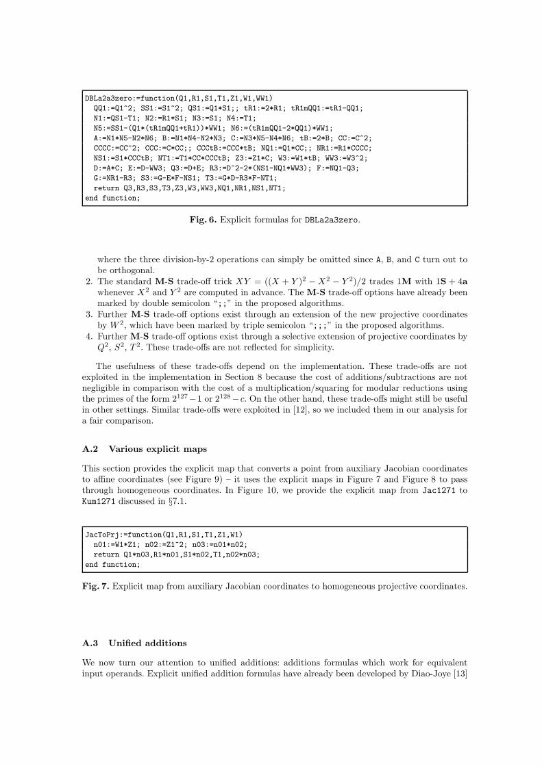
DBLa2a3zero:=function(Q1,R1,S1,T1,Z1,W1,WW1)

QQ1:=Q1^2; SS1:=S1^2; QS1:=Q1*S1;; tR1:=2*R1; tR1mQQ1:=tR1-QQ1;

N1:=QS1-T1; N2:=R1*S1; N3:=S1; N4:=T1;

N5:=SS1-(Q1*(tR1mQQ1+tR1))*WW1; N6:=(tR1mQQ1-2*QQ1)*WW1;

A:=N1*N5-N2*N6; B:=N1*N4-N2*N3; C:=N3*N5-N4*N6; tB:=2*B; CC:=C^2;

CCCC:=CC^2; CCC:=C*CC;; CCCtB:=CCC*tB; NQ1:=Q1*CC;; NR1:=R1*CCCC;

NS1:=S1*CCCtB; NT1:=T1*CC*CCCtB; Z3:=Z1*C; W3:=W1*tB; WW3:=W3^2;

D:=A*C; E:=D-WW3; Q3:=D+E; R3:=D^2-2*(NS1-NQ1*WW3); F:=NQ1-Q3;

G:=NR1-R3; S3:=G-E*F-NS1; T3:=G*D-R3*F-NT1;

return Q3,R3,S3,T3,Z3,W3,WW3,NQ1,NR1,NS1,NT1;

end function;

Fig. 6. Explicit formulas for DBLa2a3zero.

where the three division-by-2 operations can simply be omitted since A, B, and C turn out tobe orthogonal.

2. The standard M-S trade-off trick XY = ((X + Y )2 −X2 − Y 2)/2 trades 1M with 1S + 4awhenever X2 and Y 2 are computed in advance. The M-S trade-off options have already beenmarked by double semicolon “;;” in the proposed algorithms.

3. Further M-S trade-off options exist through an extension of the new projective coordinatesby W 2, which have been marked by triple semicolon “;;;” in the proposed algorithms.

4. Further M-S trade-off options exist through a selective extension of projective coordinates byQ2, S2, T 2. These trade-offs are not reflected for simplicity.

The usefulness of these trade-offs depend on the implementation. These trade-offs are notexploited in the implementation in Section 8 because the cost of additions/subtractions are notnegligible in comparison with the cost of a multiplication/squaring for modular reductions usingthe primes of the form 2127−1 or 2128−c. On the other hand, these trade-offs might still be usefulin other settings. Similar trade-offs were exploited in [12], so we included them in our analysis fora fair comparison.

A.2 Various explicit maps

This section provides the explicit map that converts a point from auxiliary Jacobian coordinatesto affine coordinates (see Figure 9) – it uses the explicit maps in Figure 7 and Figure 8 to passthrough homogeneous coordinates. In Figure 10, we provide the explicit map from Jac1271 toKum1271 discussed in §7.1.

JacToPrj:=function(Q1,R1,S1,T1,Z1,W1)

n01:=W1*Z1; n02:=Z1^2; n03:=n01*n02;

return Q1*n03,R1*n01,S1*n02,T1,n02*n03;

end function;

Fig. 7. Explicit map from auxiliary Jacobian coordinates to homogeneous projective coordinates.

A.3 Unified additions

We now turn our attention to unified additions: additions formulas which work for equivalentinput operands. Explicit unified addition formulas have already been developed by Diao-Joye [13]

PrjToAfn:=function(Q1,R1,S1,T1,Z1)

n01:=1/Z1;

return Q1*n01,R1*n01,S1*n01,T1*n01;

end function;

Fig. 8. Explicit map from homogeneous projective coordinates to affine coordinates.

JacToAfn:=function(Q1,R1,S1,T1,Z1,W1)

Q1,R1,S1,T1,Z1:=JacToPrj(Q1,R1,S1,T1,Z1,W1);

return PrjToAfn(Q1,R1,S1,T1,Z1);

end function;

Fig. 9. Explicit map from auxiliary Jacobian coordinates to affine coordinates.

/*Note1: beta is equal to -(lambda+mu+nu)/5.*/

JacToKum:=function(Q1,R1,S1,T1,Z1,W1,u,beta,a,b,c,d,lambda,mu,nu)

n01:=u*Z1; n02:=n01^2; n03:=W1*n01; n04:=n02*n03; R1:=R1*n03; S1:=S1*n02;

Q1:=Q1*n04; Z1:=n02*n04; n01:=beta*Z1; n03:=2*n01; Q1:=n03+Q1; n02:=Q1-n01;

n04:=n02*beta; R1:=n04+R1; n01:=beta*S1; T1:=n01+T1; n01:=T1^2;

n02:=lambda*Z1; n03:=mu*Z1; n04:=nu*Z1; T1:=n01*Z1; W1:=Z1+Q1; Z1:=n02+Q1;

S1:=Z1+n04; n01:=n03-R1; Q1:=n01*S1; S1:=R1*Q1; n01:=S1-T1; Q1:=a*n01;

S1:=nu*n02; n01:=S1-R1; S1:=W1+n03; n01:=n01*S1; S1:=R1*n01; n01:=S1-T1;

S1:=b*n01; n01:=Z1+n03; n03:=n04-R1; n01:=n01*n03; n03:=R1*n01; n01:=n03-T1;

Z1:=mu*n02; n03:=Z1-R1; n02:=W1+n04; W1:=R1*n03; R1:=c*n01; n01:=W1*n02;

n04:=n01-T1; T1:=d*n04; Z1:=1/Q1; S1:=S1*Z1; R1:=R1*Z1; T1:=T1*Z1;

return Q1,S1,R1; /*Note2: (X1,Y1,Z1):=(Q1,S1,R1).*/

end function;

Fig. 10. Explicit map from auxiliary Jacobian coordinates to affine Kummer coordinates.

in affine coordinates. The proposed formulas below differ from Diao-Joye’s formulas but producethe same results (see the Magma script at the end of the appendix).

With notation as in Section 6, an addition of two points can be performed by first defining thecommon subexpressions

A :=(

s22 − a2 − q2(

2r2 − q22 − a3

)

− r1 (q1 + q2))

·

(q1 (s1 + s2) − (t1 + t2)) −(

r2 − q22− a3 − q1 (q1 + q2) + r1

)

r1 (s1 + s2) ,

B := (q1 (s1 + s2) − (t1 + t2)) (t1 + t2) − r1 (s1 + s2)2,

C :=(

s22 − a2 − q2(

2r2 − q22 − a3

)

− r1 (q1 + q2))

·

(s1 + s2) − (t1 + t2)(

r2 − q22− a3 − q1 (q1 + q2) + r1

)

.

and then computing

q3 = (q2 − q1) + 2A

C−B2

C2,

r3 = (q2 − q1)A

C+A2

C2+ (q1 + q2)

B2

C2− (s1 + s2)

B

C,

s3 = (q1 − q3)A

B− q3 (q1 − q3)

C

B+ (q2 − q1) (q1 − q3)

C

B+ (r1 − r3)

C

B− s1,

t3 = (r1 − r3)A

B− r3 (q1 − q3)

C

B+ (q2 − q1) (r1 − r3)

C

B− t1.

(17)

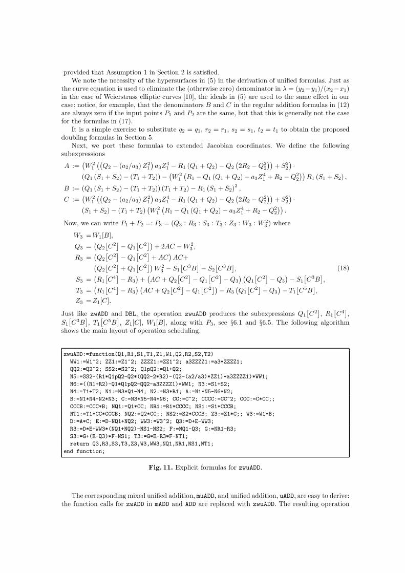
provided that Assumption 1 in Section 2 is satisfied.We note the necessity of the hypersurfaces in (5) in the derivation of unified formulas. Just as

the curve equation is used to eliminate the (otherwise zero) denominator in λ = (y2−y1)/(x2−x1)in the case of Weierstrass elliptic curves [10], the ideals in (5) are used to the same effect in ourcase: notice, for example, that the denominators B and C in the regular addition formulas in (12)are always zero if the input points P1 and P2 are the same, but that this is generally not the casefor the formulas in (17).

It is a simple exercise to substitute q2 = q1, r2 = r1, s2 = s1, t2 = t1 to obtain the proposeddoubling formulas in Section 5.

Next, we port these formulas to extended Jacobian coordinates. We define the followingsubexpressions

A :=(

W 2

1

((

Q2 − (a2/a3)Z2

1

)

a3Z4

1−R1 (Q1 +Q2) −Q2

(

2R2 −Q2

2

))

+ S2

2

)

·

(Q1 (S1 + S2) − (T1 + T2)) −(

W 2

1

(

R1 −Q1 (Q1 +Q2) − a3Z4

1+R2 −Q2

2

))

R1 (S1 + S2) ,

B := (Q1 (S1 + S2) − (T1 + T2)) (T1 + T2) −R1 (S1 + S2)2 ,

C :=(

W 2

1

((

Q2 − (a2/a3)Z2

1

)

a3Z4

1−R1 (Q1 +Q2) −Q2

(

2R2 −Q2

2

))

+ S2

2

)

·

(S1 + S2) − (T1 + T2)(

W 2

1

(

R1 −Q1 (Q1 +Q2) − a3Z4

1 +R2 −Q2

2

))

.

Now, we can write P1 + P2 =: P3 = (Q3 : R3 : S3 : T3 : Z3 : W3 : W 2

3) where

W3 =W1[B],

Q3 =(

Q2

[

C2]

−Q1

[

C2])

+ 2AC −W 2

3 ,

R3 =(

Q2

[

C2]

−Q1

[

C2]

+AC)

AC+(

Q2

[

C2]

+Q1

[

C2])

W 2

3− S1

[

C3B]

− S2

[

C3B]

,

S3 =(

R1

[

C4]

−R3

)

+(

AC +Q2

[

C2]

−Q1

[

C2]

−Q3

) (

Q1

[

C2]

−Q3

)

− S1

[

C3B]

,

T3 =(

R1

[

C4]

−R3

) (

AC +Q2

[

C2]

−Q1

[

C2])

−R3

(

Q1

[

C2]

−Q3

)

− T1

[

C5B]

,

Z3 =Z1[C].

(18)

Just like zwADD and DBL, the operation zwuADD produces the subexpressions Q1

[

C2]

, R1

[

C4]

,

S1

[

C3B]

, T1

[

C5B]

, Z1[C], W1[B], along with P3, see §6.1 and §6.5. The following algorithmshows the main layout of operation scheduling.

zwuADD:=function(Q1,R1,S1,T1,Z1,W1,Q2,R2,S2,T2)

WW1:=W1^2; ZZ1:=Z1^2; ZZZZ1:=ZZ1^2; a3ZZZZ1:=a3*ZZZZ1;

QQ2:=Q2^2; SS2:=S2^2; Q1pQ2:=Q1+Q2;

N5:=SS2-(R1*Q1pQ2-Q2*(QQ2-2*R2)-(Q2-(a2/a3)*ZZ1)*a3ZZZZ1)*WW1;

N6:=((R1+R2)-Q1*Q1pQ2-QQ2-a3ZZZZ1)*WW1; N3:=S1+S2;

N4:=T1+T2; N1:=N3*Q1-N4; N2:=N3*R1; A:=N1*N5-N6*N2;

B:=N1*N4-N2*N3; C:=N3*N5-N4*N6; CC:=C^2; CCCC:=CC^2; CCC:=C*CC;;

CCCB:=CCC*B; NQ1:=Q1*CC; NR1:=R1*CCCC; NS1:=S1*CCCB;

NT1:=T1*CC*CCCB; NQ2:=Q2*CC;; NS2:=S2*CCCB; Z3:=Z1*C;; W3:=W1*B;

D:=A*C; E:=D-NQ1+NQ2; WW3:=W3^2; Q3:=D+E-WW3;

R3:=D*E+WW3*(NQ1+NQ2)-NS1-NS2; F:=NQ1-Q3; G:=NR1-R3;

S3:=G+(E-Q3)*F-NS1; T3:=G*E-R3*F-NT1;

return Q3,R3,S3,T3,Z3,W3,WW3,NQ1,NR1,NS1,NT1;

end function;

Fig. 11. Explicit formulas for zwuADD.

The corresponding mixed unified addition, muADD, and unified addition, uADD, are easy to derive:the function calls for zwADD in mADD and ADD are replaced with zwuADD. The resulting operation

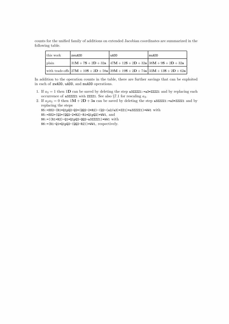
counts for the unified family of additions on extended Jacobian coordinates are summarized in thefollowing table.

this work zwuADD uADD muADD

plain 31M + 7S + 2D + 32a 47M + 12S + 2D + 32a 38M + 9S + 2D + 32a

with trade-offs 27M + 10S + 2D + 58a 39M + 19S + 2D + 74a 33M + 13S + 2D + 62a

In addition to the operation counts in the table, there are further savings that can be exploitedin each of zwADD, uADD, and muADD operations.

1. If a3 = 1 then 1D can be saved by deleting the step a3ZZZZ1:=a3*ZZZZ1 and by replacing eachoccurrence of a3ZZZZ1 with ZZZZ1. See also §7.1 for rescaling a3.

2. If a2a3 = 0 then 1M + 2D + 3a can be saved by deleting the step a3ZZZZ1:=a3*ZZZZ1 and byreplacing the stepsN5:=SS2-(R1*Q1pQ2-Q2*(QQ2-2*R2)-(Q2-(a2/a3)*ZZ1)*a3ZZZZ1)*WW1 withN5:=SS2+(Q2*(QQ2-2*R2)-R1*Q1pQ2)*WW1, andN6:=((R1+R2)-Q1*Q1pQ2-QQ2-a3ZZZZ1)*WW1 withN6:=(R1-Q1*Q1pQ2-(QQ2-R2))*WW1, respectively.

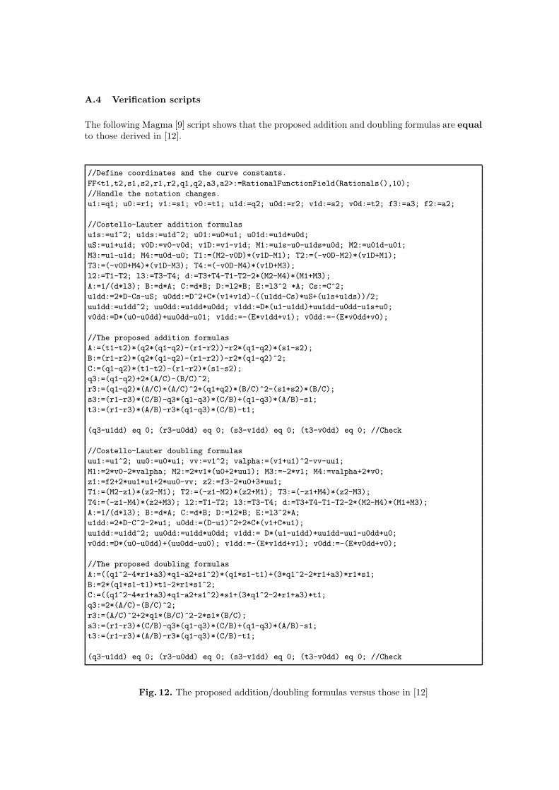
A.4 Verification scripts

The following Magma [9] script shows that the proposed addition and doubling formulas are equalto those derived in [12].

//Define coordinates and the curve constants.

FF<t1,t2,s1,s2,r1,r2,q1,q2,a3,a2>:=RationalFunctionField(Rationals(),10);

//Handle the notation changes.

u1:=q1; u0:=r1; v1:=s1; v0:=t1; u1d:=q2; u0d:=r2; v1d:=s2; v0d:=t2; f3:=a3; f2:=a2;

//Costello-Lauter addition formulas

u1s:=u1^2; u1ds:=u1d^2; u01:=u0*u1; u01d:=u1d*u0d;

uS:=u1+u1d; v0D:=v0-v0d; v1D:=v1-v1d; M1:=u1s-u0-u1ds+u0d; M2:=u01d-u01;

M3:=u1-u1d; M4:=u0d-u0; T1:=(M2-v0D)*(v1D-M1); T2:=(-v0D-M2)*(v1D+M1);

T3:=(-v0D+M4)*(v1D-M3); T4:=(-v0D-M4)*(v1D+M3);

l2:=T1-T2; l3:=T3-T4; d:=T3+T4-T1-T2-2*(M2-M4)*(M1+M3);

A:=1/(d*l3); B:=d*A; C:=d*B; D:=l2*B; E:=l3^2 *A; Cs:=C^2;

u1dd:=2*D-Cs-uS; u0dd:=D^2+C*(v1+v1d)-((u1dd-Cs)*uS+(u1s+u1ds))/2;

uu1dd:=u1dd^2; uu0dd:=u1dd*u0dd; v1dd:=D*(u1-u1dd)+uu1dd-u0dd-u1s+u0;

v0dd:=D*(u0-u0dd)+uu0dd-u01; v1dd:=-(E*v1dd+v1); v0dd:=-(E*v0dd+v0);

//The proposed addition formulas

A:=(t1-t2)*(q2*(q1-q2)-(r1-r2))-r2*(q1-q2)*(s1-s2);

B:=(r1-r2)*(q2*(q1-q2)-(r1-r2))-r2*(q1-q2)^2;

C:=(q1-q2)*(t1-t2)-(r1-r2)*(s1-s2);

q3:=(q1-q2)+2*(A/C)-(B/C)^2;

r3:=(q1-q2)*(A/C)+(A/C)^2+(q1+q2)*(B/C)^2-(s1+s2)*(B/C);

s3:=(r1-r3)*(C/B)-q3*(q1-q3)*(C/B)+(q1-q3)*(A/B)-s1;

t3:=(r1-r3)*(A/B)-r3*(q1-q3)*(C/B)-t1;

(q3-u1dd) eq 0; (r3-u0dd) eq 0; (s3-v1dd) eq 0; (t3-v0dd) eq 0; //Check

//Costello-Lauter doubling formulas

uu1:=u1^2; uu0:=u0*u1; vv:=v1^2; valpha:=(v1+u1)^2-vv-uu1;

M1:=2*v0-2*valpha; M2:=2*v1*(u0+2*uu1); M3:=-2*v1; M4:=valpha+2*v0;

z1:=f2+2*uu1*u1+2*uu0-vv; z2:=f3-2*u0+3*uu1;

T1:=(M2-z1)*(z2-M1); T2:=(-z1-M2)*(z2+M1); T3:=(-z1+M4)*(z2-M3);

T4:=(-z1-M4)*(z2+M3); l2:=T1-T2; l3:=T3-T4; d:=T3+T4-T1-T2-2*(M2-M4)*(M1+M3);

A:=1/(d*l3); B:=d*A; C:=d*B; D:=l2*B; E:=l3^2*A;

u1dd:=2*D-C^2-2*u1; u0dd:=(D-u1)^2+2*C*(v1+C*u1);

uu1dd:=u1dd^2; uu0dd:=u1dd*u0dd; v1dd:= D*(u1-u1dd)+uu1dd-uu1-u0dd+u0;

v0dd:=D*(u0-u0dd)+(uu0dd-uu0); v1dd:=-(E*v1dd+v1); v0dd:=-(E*v0dd+v0);

//The proposed doubling formulas

A:=((q1^2-4*r1+a3)*q1-a2+s1^2)*(q1*s1-t1)+(3*q1^2-2*r1+a3)*r1*s1;

B:=2*(q1*s1-t1)*t1-2*r1*s1^2;

C:=((q1^2-4*r1+a3)*q1-a2+s1^2)*s1+(3*q1^2-2*r1+a3)*t1;

q3:=2*(A/C)-(B/C)^2;

r3:=(A/C)^2+2*q1*(B/C)^2-2*s1*(B/C);

s3:=(r1-r3)*(C/B)-q3*(q1-q3)*(C/B)+(q1-q3)*(A/B)-s1;

t3:=(r1-r3)*(A/B)-r3*(q1-q3)*(C/B)-t1;

(q3-u1dd) eq 0; (r3-u0dd) eq 0; (s3-v1dd) eq 0; (t3-v0dd) eq 0; //Check

Fig. 12. The proposed addition/doubling formulas versus those in [12]

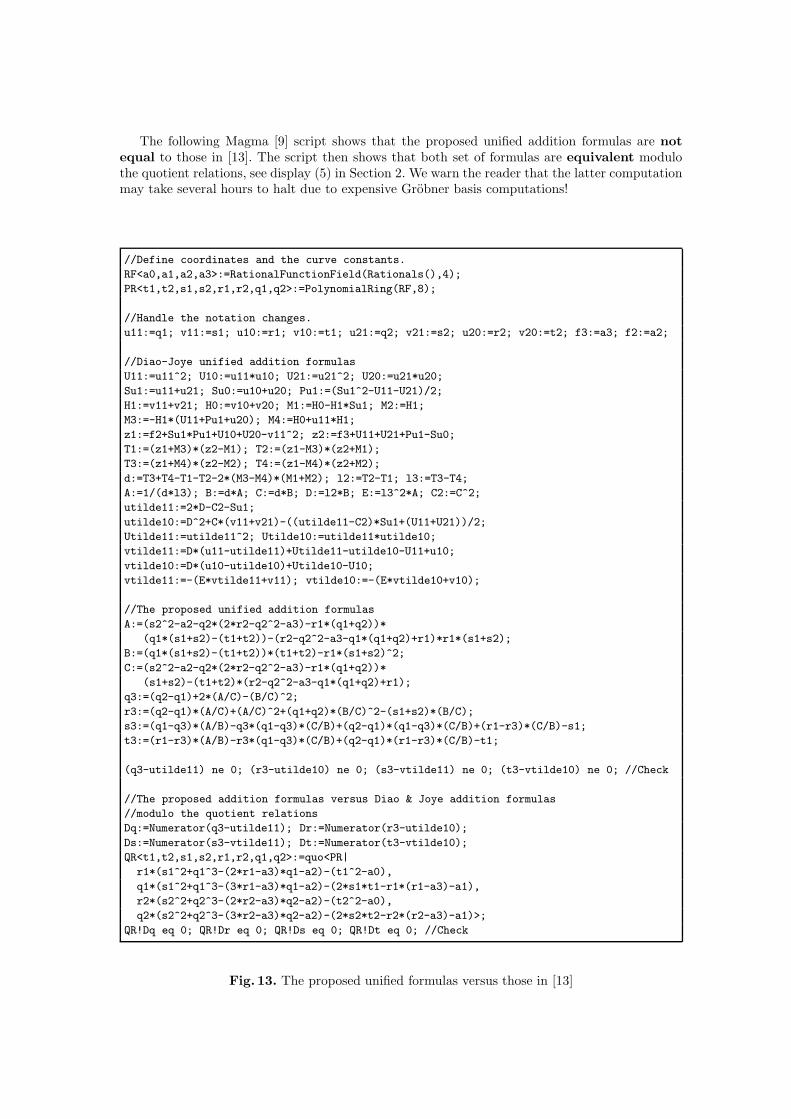
The following Magma [9] script shows that the proposed unified addition formulas are notequal to those in [13]. The script then shows that both set of formulas are equivalent modulothe quotient relations, see display (5) in Section 2. We warn the reader that the latter computationmay take several hours to halt due to expensive Grobner basis computations!

//Define coordinates and the curve constants.

RF<a0,a1,a2,a3>:=RationalFunctionField(Rationals(),4);

PR<t1,t2,s1,s2,r1,r2,q1,q2>:=PolynomialRing(RF,8);

//Handle the notation changes.

u11:=q1; v11:=s1; u10:=r1; v10:=t1; u21:=q2; v21:=s2; u20:=r2; v20:=t2; f3:=a3; f2:=a2;

//Diao-Joye unified addition formulas

U11:=u11^2; U10:=u11*u10; U21:=u21^2; U20:=u21*u20;

Su1:=u11+u21; Su0:=u10+u20; Pu1:=(Su1^2-U11-U21)/2;

H1:=v11+v21; H0:=v10+v20; M1:=H0-H1*Su1; M2:=H1;

M3:=-H1*(U11+Pu1+u20); M4:=H0+u11*H1;

z1:=f2+Su1*Pu1+U10+U20-v11^2; z2:=f3+U11+U21+Pu1-Su0;

T1:=(z1+M3)*(z2-M1); T2:=(z1-M3)*(z2+M1);

T3:=(z1+M4)*(z2-M2); T4:=(z1-M4)*(z2+M2);

d:=T3+T4-T1-T2-2*(M3-M4)*(M1+M2); l2:=T2-T1; l3:=T3-T4;

A:=1/(d*l3); B:=d*A; C:=d*B; D:=l2*B; E:=l3^2*A; C2:=C^2;

utilde11:=2*D-C2-Su1;

utilde10:=D^2+C*(v11+v21)-((utilde11-C2)*Su1+(U11+U21))/2;

Utilde11:=utilde11^2; Utilde10:=utilde11*utilde10;

vtilde11:=D*(u11-utilde11)+Utilde11-utilde10-U11+u10;

vtilde10:=D*(u10-utilde10)+Utilde10-U10;

vtilde11:=-(E*vtilde11+v11); vtilde10:=-(E*vtilde10+v10);

//The proposed unified addition formulas

A:=(s2^2-a2-q2*(2*r2-q2^2-a3)-r1*(q1+q2))*

(q1*(s1+s2)-(t1+t2))-(r2-q2^2-a3-q1*(q1+q2)+r1)*r1*(s1+s2);

B:=(q1*(s1+s2)-(t1+t2))*(t1+t2)-r1*(s1+s2)^2;

C:=(s2^2-a2-q2*(2*r2-q2^2-a3)-r1*(q1+q2))*

(s1+s2)-(t1+t2)*(r2-q2^2-a3-q1*(q1+q2)+r1);

q3:=(q2-q1)+2*(A/C)-(B/C)^2;

r3:=(q2-q1)*(A/C)+(A/C)^2+(q1+q2)*(B/C)^2-(s1+s2)*(B/C);

s3:=(q1-q3)*(A/B)-q3*(q1-q3)*(C/B)+(q2-q1)*(q1-q3)*(C/B)+(r1-r3)*(C/B)-s1;

t3:=(r1-r3)*(A/B)-r3*(q1-q3)*(C/B)+(q2-q1)*(r1-r3)*(C/B)-t1;

(q3-utilde11) ne 0; (r3-utilde10) ne 0; (s3-vtilde11) ne 0; (t3-vtilde10) ne 0; //Check

//The proposed addition formulas versus Diao & Joye addition formulas

//modulo the quotient relations

Dq:=Numerator(q3-utilde11); Dr:=Numerator(r3-utilde10);

Ds:=Numerator(s3-vtilde11); Dt:=Numerator(t3-vtilde10);

QR<t1,t2,s1,s2,r1,r2,q1,q2>:=quo<PR|

r1*(s1^2+q1^3-(2*r1-a3)*q1-a2)-(t1^2-a0),

q1*(s1^2+q1^3-(3*r1-a3)*q1-a2)-(2*s1*t1-r1*(r1-a3)-a1),

r2*(s2^2+q2^3-(2*r2-a3)*q2-a2)-(t2^2-a0),

q2*(s2^2+q2^3-(3*r2-a3)*q2-a2)-(2*s2*t2-r2*(r2-a3)-a1)>;

QR!Dq eq 0; QR!Dr eq 0; QR!Ds eq 0; QR!Dt eq 0; //Check

Fig. 13. The proposed unified formulas versus those in [13]