Jackknife Empirical Likelihood Inference For The … EMPIRICAL LIKELIHOOD INFERENCE FOR THE PIETRA RATIO by YUEJU SU Under the Direction of Yichuan Zhao, PhD ABSTRACT Pietra ratio

Georgia State UniversityScholarWorks @ Georgia State University

Mathematics Theses Department of Mathematics and Statistics

12-17-2014

Jackknife Empirical Likelihood Inference For ThePietra RatioYueju Su

Follow this and additional works at: http://scholarworks.gsu.edu/math_theses

This Thesis is brought to you for free and open access by the Department of Mathematics and Statistics at ScholarWorks @ Georgia State University. Ithas been accepted for inclusion in Mathematics Theses by an authorized administrator of ScholarWorks @ Georgia State University. For moreinformation, please contact [email protected].

Recommended CitationSu, Yueju, "Jackknife Empirical Likelihood Inference For The Pietra Ratio." Thesis, Georgia State University, 2014.http://scholarworks.gsu.edu/math_theses/140

http://scholarworks.gsu.edu?utm_source=scholarworks.gsu.edu%2Fmath_theses%2F140&utm_medium=PDF&utm_campaign=PDFCoverPages

http://scholarworks.gsu.edu/math_theses?utm_source=scholarworks.gsu.edu%2Fmath_theses%2F140&utm_medium=PDF&utm_campaign=PDFCoverPages

http://scholarworks.gsu.edu/math?utm_source=scholarworks.gsu.edu%2Fmath_theses%2F140&utm_medium=PDF&utm_campaign=PDFCoverPages

http://scholarworks.gsu.edu/math_theses?utm_source=scholarworks.gsu.edu%2Fmath_theses%2F140&utm_medium=PDF&utm_campaign=PDFCoverPages

mailto:[email protected]

JACKKNIFE EMPIRICAL LIKELIHOOD INFERENCE FOR THE PIETRA RATIO

by

YUEJU SU

Under the Direction of Yichuan Zhao, PhD

ABSTRACT

Pietra ratio (Pietra index), also known as Robin Hood index, Schutz coefficient (Ricci-

Schutz index) or half the relative mean deviation, is a good measure of statistical hetero-

geneity in the context of positive-valued data sets. In this thesis, two novel methods namely

“adjusted jackknife empirical likelihood” and “extended jackknife empirical likelihood” are

developed from the jackknife empirical likelihood method to obtain interval estimation of

the Pietra ratio of a population. The performance of the two novel methods are compared

with the jackknife empirical likelihood method, the normal approximation method and two

bootstrap methods (the percentile bootstrap method and the bias corrected and accelerated

bootstrap method). Simulation results indicate that under both symmetric and skewed dis-

tributions, especially when the sample is small, the extended jackknife empirical likelihood

method gives the best performance among the six methods in terms of the coverage proba-

bilities and interval lengths of the confidence interval of Pietra ratio; when the sample size is

over 20, the adjusted jackknife empirical likelihood method performs better than the other

methods, except the extended jackknife empirical likelihood method. Furthermore, several

real data sets are used to illustrate the proposed methods.

INDEX WORDS: Bootstrap method, Coverage probability, Jackknife empirical likeli-hood, Adjusted jackknife empirical likelihood, Extended jackknife em-pirical likelihood


by

YUEJU SU

A Dissertation Submitted in Partial Fulfillment of the Requirements for the Degree of

Master of Science

in the College of Arts and Sciences

Georgia State University

2014

Copyright byYueju Su

2014


by

YUEJU SU

Committee Chair: Yichuan Zhao

Committee: Jing Zhang

Xin Qi

Electronic Version Approved:

Office of Graduate Studies

College of Arts and Sciences

Georgia State University

December 2014

iv

DEDICATION

This thesis is dedicated to Georgia State University.

v

ACKNOWLEDGEMENTS

This thesis work would not have been possible without the support of many people.

Here I would like to acknowledge those who have helped me in the completion of this thesis.

First and foremost I want to express my sincere gratitude to my advisor Professor,

Yichuan Zhao, who is a patient and intellectual man. There is no way I could have complet-

ed my thesis successfully without his patient guidance and generous support. He guided me

through all the intricacies of empirical likelihood methods.

I am very grateful to Dr. Xin Qi, who provided a lot of guidance for my programming

part, without his help I could not accomplish my simulation study.

I am also grateful to the other members of my thesis committee for taking the time to

proofread and add valuable input to my thesis.

Many others helped along the way. I would like to thank all the other professors and

staffs in the Mathematics Statistics department of Georgia State University for their support

and guidance. Without their help, I could not complete the requirements of the graduate

program. In addition, I would like to thank my classmates Songling Shan, Xueping Meng,

and Bing Liu for their help on the use of Latex.

I would also like to express my great appreciation to Professor Ruiyan Luo in the School

of Public Health of Georgia State University, Professor Jiandong Li and Professor Andrew

Gewirtz in the Biology department of Georgia State University for their financial support,

without which I would not have been able to complete this program of study.

I am especially grateful to my family: my parents, husband and lovely son, for support-

ing me throughout my life. I love you all forever.

vi

TABLE OF CONTENTS

ACKNOWLEDGEMENTS . . . . . . . . . . . . . . . . . v

LIST OF TABLES . . . . . . . . . . . . . . . . . . . . viii

LIST OF FIGURES . . . . . . . . . . . . . . . . . . . . ix

LIST OF ABBREVIATIONS . . . . . . . . . . . . . . . . x

CHAPTER 1 INTRODUCTION . . . . . . . . . . . . . . . 1

CHAPTER 2 METHODOLOGY . . . . . . . . . . . . . . . 5

2.1 Normal approximation method for P . . . . . . . . . . . . . . . . . 5

2.2 Bootstrap methods for P . . . . . . . . . . . . . . . . . . . . . . . . . 6

2.3 Review of empirical likelihood . . . . . . . . . . . . . . . . . . . . . 8

2.4 Jackknife empirical likelihood for P . . . . . . . . . . . . . . . . . . 9

2.5 Adjusted jackknife empirical likelihood for P . . . . . . . . . . . . 11

2.6 Extended jackknife empirical likelihood for P . . . . . . . . . . . . 12

CHAPTER 3 SIMULATION STUDY . . . . . . . . . . . . . 15

3.1 Simulation study under the normal distribution . . . . . . . . . . 15

3.2 Simulation study under the t distribution . . . . . . . . . . . . . . 17

3.3 Simulation study under the exponential distribution . . . . . . . 17

3.4 Simulation study under the gamma distribution . . . . . . . . . . 19

3.5 Conclusion . . . . . . . . . . . . . . . . . . . . . . . . . . . . . . . . . . 20

CHAPTER 4 REAL DATA ANALYSIS . . . . . . . . . . . . 25

4.1 Airmiles data analysis . . . . . . . . . . . . . . . . . . . . . . . . . . . 26

4.2 White income data analysis . . . . . . . . . . . . . . . . . . . . . . . 27

vii

4.3 Housefly wing data analysis . . . . . . . . . . . . . . . . . . . . . . . 28

4.4 Conclusion . . . . . . . . . . . . . . . . . . . . . . . . . . . . . . . . . . 28

CHAPTER 5 SUMMARY AND FUTURE WORK . . . . . . . . 30

5.1 Summary . . . . . . . . . . . . . . . . . . . . . . . . . . . . . . . . . . . 30

5.2 Future Work . . . . . . . . . . . . . . . . . . . . . . . . . . . . . . . . 30

REFERENCES . . . . . . . . . . . . . . . . . . . . . 32

APPENDICES . . . . . . . . . . . . . . . . . . . . . . 36

Appendix A ROBIN HOOD INDEX . . . . . . . . . . . . . 36

Appendix B THE HISTOGRAMS OF REAL DATA SETS . . . . 37

viii

LIST OF TABLES

Table 3.1 : Coverage probability under the normal distribution . . . . . . . 17

Table 3.2 : Average length of CI under the normal distribution . . . . . . . 18

Table 3.3 : Coverage probability under the t distribution . . . . . . . . . . 19

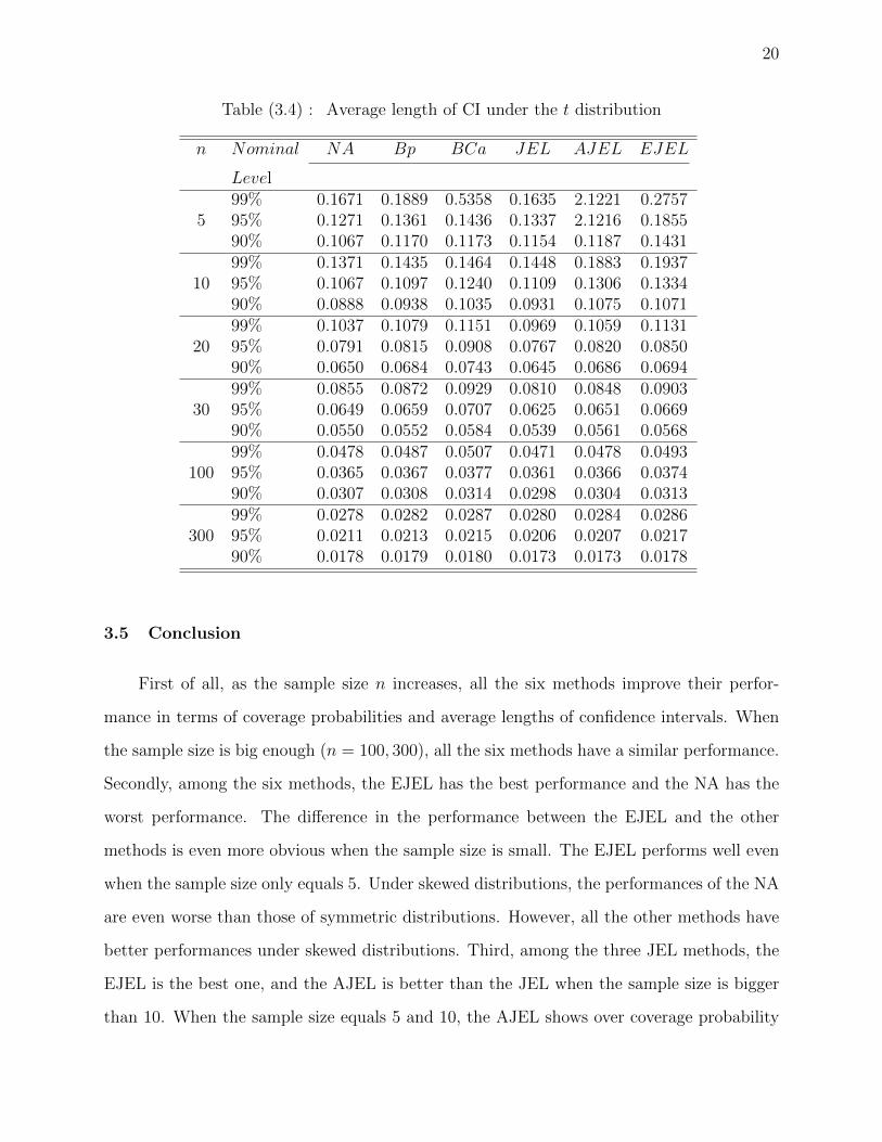
Table 3.4 : Average length of CI under the t distribution . . . . . . . . . . 20

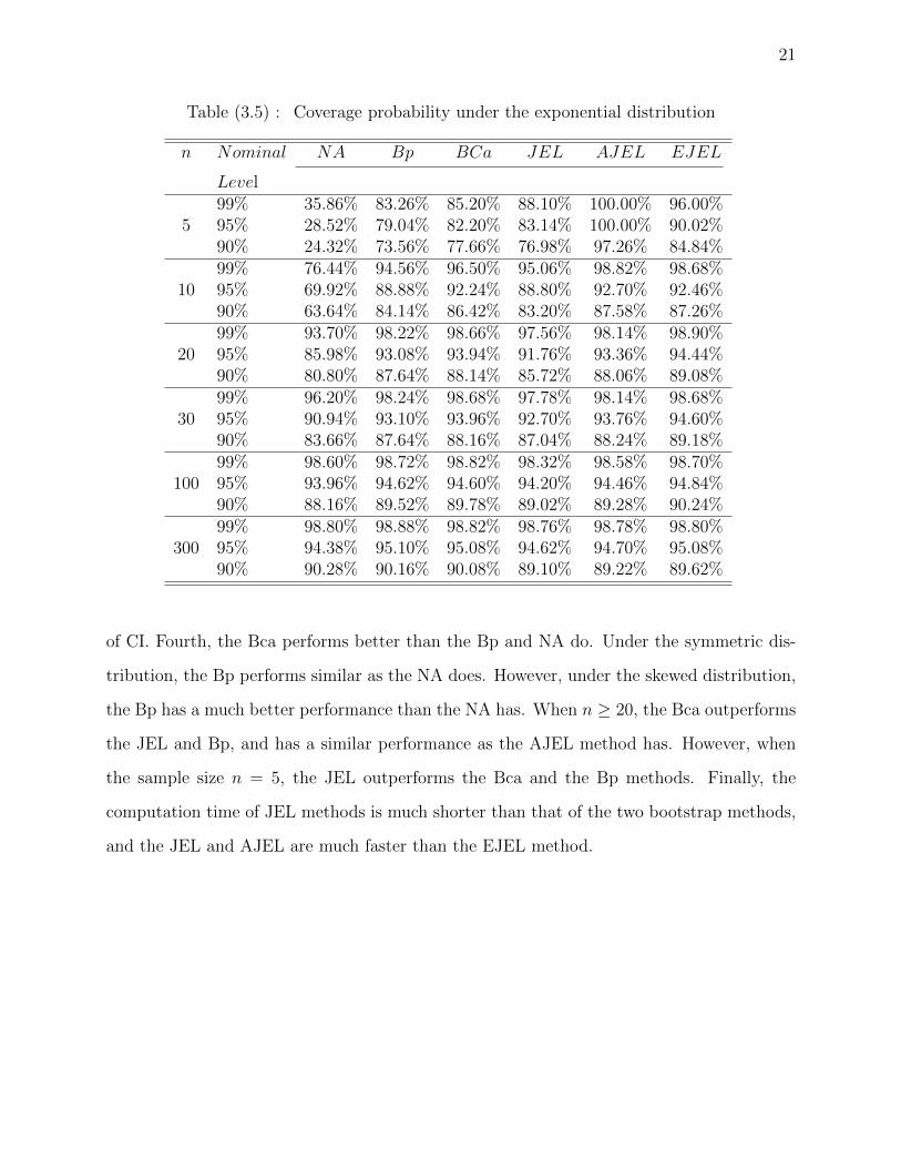
Table 3.5 : Coverage probability under the exponential distribution . . . . 21

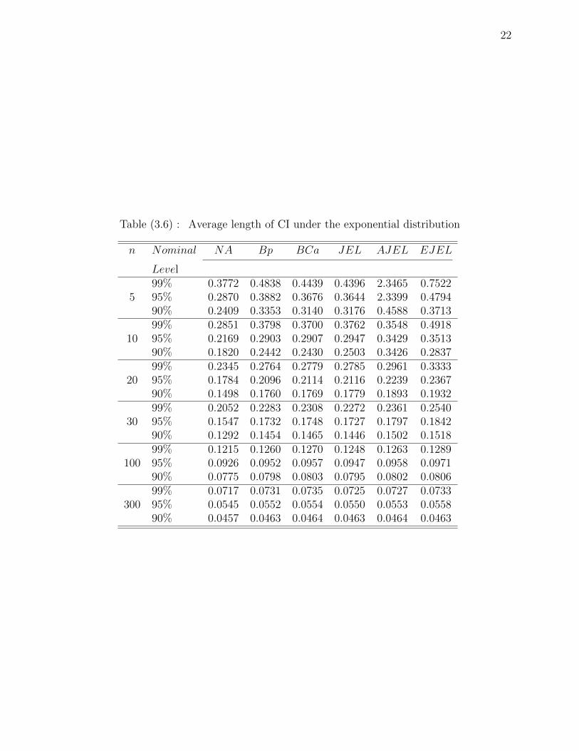
Table 3.6 : Average length of CI under the exponential distribution . . . . 22

Table 3.7 : Coverage probability under the gamma distribution . . . . . . . 23

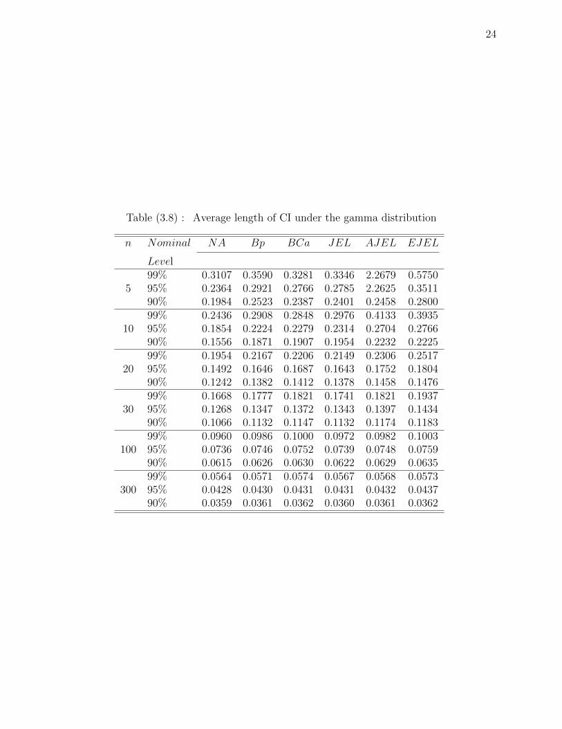
Table 3.8 : Average length of CI under the gamma distribution . . . . . . . 24

Table 4.1 : CI of Pietra ratio for airmiles data set . . . . . . . . . . . . . . 26

Table 4.2 : CI of Pietra ratio for white income data set . . . . . . . . . . . 27

Table 4.3 : CI of Pietra ratio for housefly wing data set . . . . . . . . . . 28

ix

LIST OF FIGURES

FigureA.1 Lorenz curve, relates the cumulative proportion of income to the cu-

mulative proportion of individuals, is the dot line shown on the figure.

Robin Hood index (line section DP on the figure) is the maximum ver-

tical distance between the Lorenz curve and the equal line of incomes

(line OB). . . . . . . . . . . . . . . . . . . . . . . . . . . . . . . . 36

FigureB.1 Histograms of Real Data Sets. . . . . . . . . . . . . . . . . . . . . 37

x

LIST OF ABBREVIATIONS

• P - Pietra Ratio

• NA - Normal Approximation method

• Bp - Percentile Bootstrap method

• Bca - Bias Corrected and Accelerated bootstrap method

• EL - Empirical Likelihood

• JEL - Jackknife Empirical Likelihood

• AEL - Adjusted Empirical Likelihood

• EEL - Extended Empirical Likelihood

• AJEL - Adjusted Jackknife Empirical Likelihood

• EJEL - Extended Jackknife Empirical Likelihood

• CI - Confidence Interval

• LB - Lower Bound of CI

• UB - Upper Bound of CI

1

CHAPTER 1

INTRODUCTION

Pietra ratio (Pietra index), also known as the Robin Hood index, Schutz coefficient

(Ricci-Schutz index) or half the relative mean deviation, is a quantitative measure of statis-

tical heterogeneity in the context of positive-valued random variables (Schutz (1951); Maio

(2007); Habib (2012); Salverda et al. (2009)). It is especially useful in the case of asymmetric

and skewed probability laws, and in case of asymptotically Paretian laws with finite mean

and infinite variance(Eliazar and Sokolov (2010)). It stands for the amount of the resource

that needs to be taken from more affluent areas and given to the less affluent areas in order

to achieve an equal distribution in effect (to rob the rich and give to the poor) (Schutz

(1951); Habib (2012)). In econometrics, Pietra ratio is used to measure the income inequal-

ity. Within the context of financial derivatives, the interpretation of the Pietra ratio implies

that derivative markets, in fact, people use the Pietra ratio as their benchmark measure of

statistical heterogeneity (Eliazar and Sokolov (2010)). The Pietra ratio also has been used to

study the relationship between the income inequality and the mortality in the United States

(Kennedy et al. (1996); Shi et al. (2003); Sohler et al. (2003)). In this thesis, we study

the Pietra ratio of the income data set to check the income inequality among young white

people (age from 25-30) in the United States in 2013 [see Chapter 4 for the detailed analysis].

The Pietra ratio is equivalent to the maximum vertical distance between the Lorenz curve

and the egalitarian line [see Appendix A] (Maio (2007); Salverda et al. (2009); Eliazar and

Sokolov (2010)), or the ratio of the area of the largest triangle that can be inscribed in the

region of concentration in a Lorenz diagram to the area under the line of equality (Kendall

and Stuart (1963)). Let X denote a random variable, the Pietra ratio is defined by the ratio

2

of mean deviation to two times mean:

P =1

2µ

∫ ∞−∞|X − µ|dF (X),

where P denotes Pietra ratio, µ = E(X). For the income population, X ∈ (0,∞).

In order to get a valid Pietra ratio from actual samples, one needs to know the sampling

distribution of the statistic used to estimate the parameter. For large samples, Gastwirth

(1974) established the normal approximation (NA) method for estimating the Pietra ratio.

The NA method is not only too complicated but also inadequate to be satisfactory for the

small samples. Thus, in this thesis, we adopt bootstrap and other nonparametric methods

such as empirical likelihood methods to improve the performance. The empirical likelihood

(EL) method (Owen (1988); Owen (1990)) combines the reliability of nonparametric meth-

ods with the effectiveness of the likelihood approach, which yields the confidence regions that

respect the boundaries of the support of the target parameter. The regions are invariant

under transformations and often behave better than the confidence regions obtained from

the NA method when the sample size is small (Chen and Keilegom (2009)).

According to Jing et al. (2009), the EL involves maximizing nonparametric likelihood

supported on the data subject to some constraints. And it is very easy to apply the EL

on computation when the constraints are either linear or can be linearized. However, the

EL method soon loses its appeal in other applications involving nonlinear statistics, such

as U-statistics. It becomes increasingly difficult as the sample size gets larger. The jack-

knife empirical likelihood (JEL) method (Jing et al. (2009)) combines two of the popular

nonparametric approaches: the jackknife and the empirical likelihood, turning the statistic

of interest into a sample mean based on jackknife pseudo-values (Quenouille (1956)), and

applying Owen’s empirical likelihood for the mean of the jackknife pseudo-values. The JEL

method is simple and useful in handling the more general class of statistics than U-statistics

(Jing et al. (2009)). Many new research works about JEL have been developed recently.

Gong et al. (2010) proposed JEL for the ROC curves, which enhanced the computational

3

efficiency. Adimari and Chiogna (2012) proposed the JEL method on the partial area under

the ROC curve and the difference between two partial areas under ROC curves, and shows

the JEL method performs better than the NA and the logit NA methods. Yang and Zhao

(2013) employed the JEL method to construct confidence intervals for the difference of two

correlated continuous-scale ROC curves, and shows that the JEL has good performance in

small samples with a moderate computational cost. According to Wang et al. (2013), the

JEL test for the equality of two high dimensional means shows that it has a very robust size

across dimensions and has good power. Bouadoumou et al. (2014) employed JEL method to

obtain interval estimate for the regression parameter in the accelerated failure time model

with censored observations. They found the JEL method has a better performance than the

Wald-type procedure and the existing empirical likelihood methods.

When the sample size is small and/or the dimension of the accompanying estimating

equations is high, the coverage probabilities of the EL confidence regions are often lower

than the nominal level (Owen (2001); Liu and Chen (2010)). In addition, the EL may not

be properly defined because of the so-called empty set problem (Chen et al. (2008); Tsao

and Wu (2013)). A number of approaches have been proposed to improve the accuracy of

the EL confidence regions and to address the empty set problem. The Bootstrap calibration

(Owen (1988)) and the Bartlett correction (Chen and Cui (2007)) approaches can improve

the accuracy of the EL confidence region. The adjusted empirical likelihood (AEL) (Chen

et al. (2008); Liu and Chen (2010); Chen and Liu (2012); Wang et al. (2014)) tackles both

problems simultaneously. Based on the EL method, another optimized method, the extended

empirical likelihood (EEL) method has been developed by Tsao and Wu (2013). The AEL

adds one or two pseudo-observations to the sample to ensure that the convex hull constraint

is never violated. By doing so, the AEL not only reduces the error rates of the proposed

empirical likelihood ratio but also computes more quickly compared with the profile empir-

ical likelihood method. The EEL expands the EL domain geometrically to overcome the

drawback and the mismatch. The AEL and the EEL have the same asymptotic distribution

as the EL has, but the EEL is a more natural generalization of the original EL as it also has

4

identically shaped contours as the original EL has.

Since the estimate of Pietra ratio is a nonlinear functional, the classical EL method can-

not be applied directly. We adopt the JEL method to make inference about the Pietra ratio.

In this thesis, the jackknife method is combined with either the AEL or the EEL method

separately to build two novel methods: adjusted JEL and extended JEL, for the estimation

of Pietra ratio from a sample. Their improved performances are illustrated through compar-

ing with the NA method and two of the most popular non-parametric bootstrap methods:

the percentile bootstrap method and the bias corrected and accelerated bootstrap method.

The differences among these three JEL methods are also described.

The remaining thesis is organized as follows. In Chapter 2, the employment of the

normal approximation method, bootstrap methods, jackknife empirical likelihood, adjusted

jackknife empirical likelihood (AJEL) and extended jackknife empirical likelihood (EJEL)

methods for the Pietra ratio from a sample are introduced. All the formulas applied in the

simulation study of this thesis are provided as well. Chapter 3 focuses on the simulation

study, in which the three different types of JEL methods: JEL, AJEL, and EJEL, the NA

method as well as two bootstrap methods are compared in terms of their coverage prob-

abilities and average lengths of confidence intervals under the normal (mean equals 4 and

variance equals 1), t (degree freedom equals 10, mean equals 4), exponential (λ = 1) and

gamma distributions (both scale and shape equal 2). To illustrate their better performance,

these two novel methods are employed to analyze several real data sets in Chapter 4. In

Chapter 5, the advantages and the application of these two proposed methods are discussed.

In addition, future works on these two innovative methods are discussed.

5

CHAPTER 2

METHODOLOGY

2.1 Normal approximation method for P

One measure of spread of a cumulative distribution function F(X) with random variable

X is their absolute mean deviation proposed by Gastwirth (1974) as follows:

δ=

∫ ∞−∞|x−µ| dF(x) = E |X− E(X)| . (2.1)

Let X1, X2 . . . Xn be a sequence of i.i.d. random variables with the mean µ = E(X) and

variance σ2 = E(X − µ)2. Gastwirth (1974) defined δ as an empirical estimator of δ :

δ = n−1

n∑1

∣∣Xi − X∣∣ , (2.2)

where X=n−1∑n

i=1 Xi.

After defining the sample Pietra ratio as P = δ/(2X) , Gastwirth (1974) proved that

the sample Pietra ratio P is asymptotically normally distributed with mean δ/ (2µ) and

variance

1

n

{υ2

µ2+δ2σ2

4µ4− δ

µ3

[pσ2 −

∫ µ

−∞(x− µ)2 dF (x)

]}, (2.3)

where υ2 is given by

υ2 = p2

∫ ∞µ

(x− µ)2 dF (x) +(1− p2

) ∫ µ

−∞(x− µ)2 dF (x)− δ2

4, (2.4)

and

p = F (µ) . (2.5)

6

Then we construct a 100(1 − α)% normal approximation based confidence interval for

the Pietra ratio P :

R ={P : P ± Za/2 ∗ SE

}(2.6)

and

SE =

√√√√√ 1

n

υ2

X2+δ2σ2

4X4− δ

X3

pσ2 − 1

n

∑Xi<X

(Xi − X

)2

, (2.7)

where p = Fn(X), σ2 is the variance of Xi, υ2 is the estimator of υ2, and calculated by the

following formula:

υ2 =1

np2∑Xi≥X

(Xi − X

)2+

1

n

(1− p2

) ∑Xi<X

(Xi − X

)2 − δ2

4. (2.8)

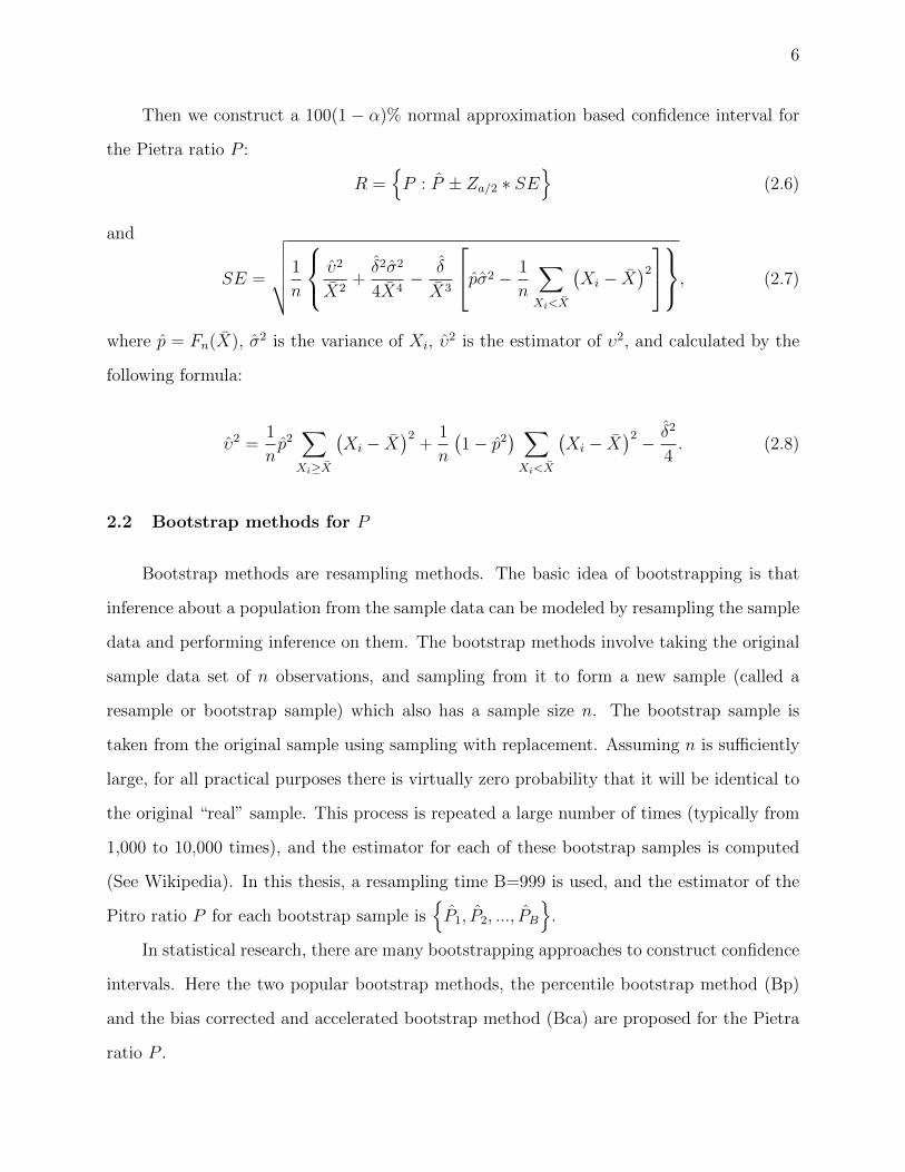
2.2 Bootstrap methods for P

Bootstrap methods are resampling methods. The basic idea of bootstrapping is that

inference about a population from the sample data can be modeled by resampling the sample

data and performing inference on them. The bootstrap methods involve taking the original

sample data set of n observations, and sampling from it to form a new sample (called a

resample or bootstrap sample) which also has a sample size n. The bootstrap sample is

taken from the original sample using sampling with replacement. Assuming n is sufficiently

large, for all practical purposes there is virtually zero probability that it will be identical to

the original “real” sample. This process is repeated a large number of times (typically from

1,000 to 10,000 times), and the estimator for each of these bootstrap samples is computed

(See Wikipedia). In this thesis, a resampling time B=999 is used, and the estimator of the

Pitro ratio P for each bootstrap sample is{P1, P2, ..., PB

}.

In statistical research, there are many bootstrapping approaches to construct confidence

intervals. Here the two popular bootstrap methods, the percentile bootstrap method (Bp)

and the bias corrected and accelerated bootstrap method (Bca) are proposed for the Pietra

ratio P .

7

For the Bp method, the 1−α confidence interval for the Pietra ratio is defined as follows

(Wang and Zhao (2009)),

P ∈[P ∗α/2, P

∗1−α/2

], (2.9)

where P ∗α/2 and P ∗1−α/2 are obtained from the ordered bootstrap sample estimators:

{P ∗1 , P

∗2 , ..., P

∗B

}, (2.10)

and P ∗1 ≤ P ∗2 ... ≤ P ∗B, where P ∗α/2 is the B ∗ α2− th element in the ordered B elements, and

P ∗1−α/2 is the B ∗ (1− α2)− th element.

The bias corrected and accelerated bootstrap method (Bca) was introduced by Efron

(1987). Based on Efron (1987) and Carpenter and Bithell (2000), the Bca bootstrap 1 − α

level confidence interval for P is of the form

P ∈[P ∗L, P

∗U

], (2.11)

where P ∗L and P ∗U are obtained from the ordered bootstrap sample estimators. The values of

L and U are chosen to have the same cumulative probabilities as zL and zU ,

zL =z0 − z1−α/2

1− b(z0 − z1−α/2

) + z0 (2.12)

and

zU =z0 + z1−α/2

1− b(z0 + z1−α/2

) + z0, (2.13)

where z0 produces median unbiasedness and is defined by Prob (Z ≤ z0) = p0. According to

Carpenter and Bithell (2000), the value of b is obtained by

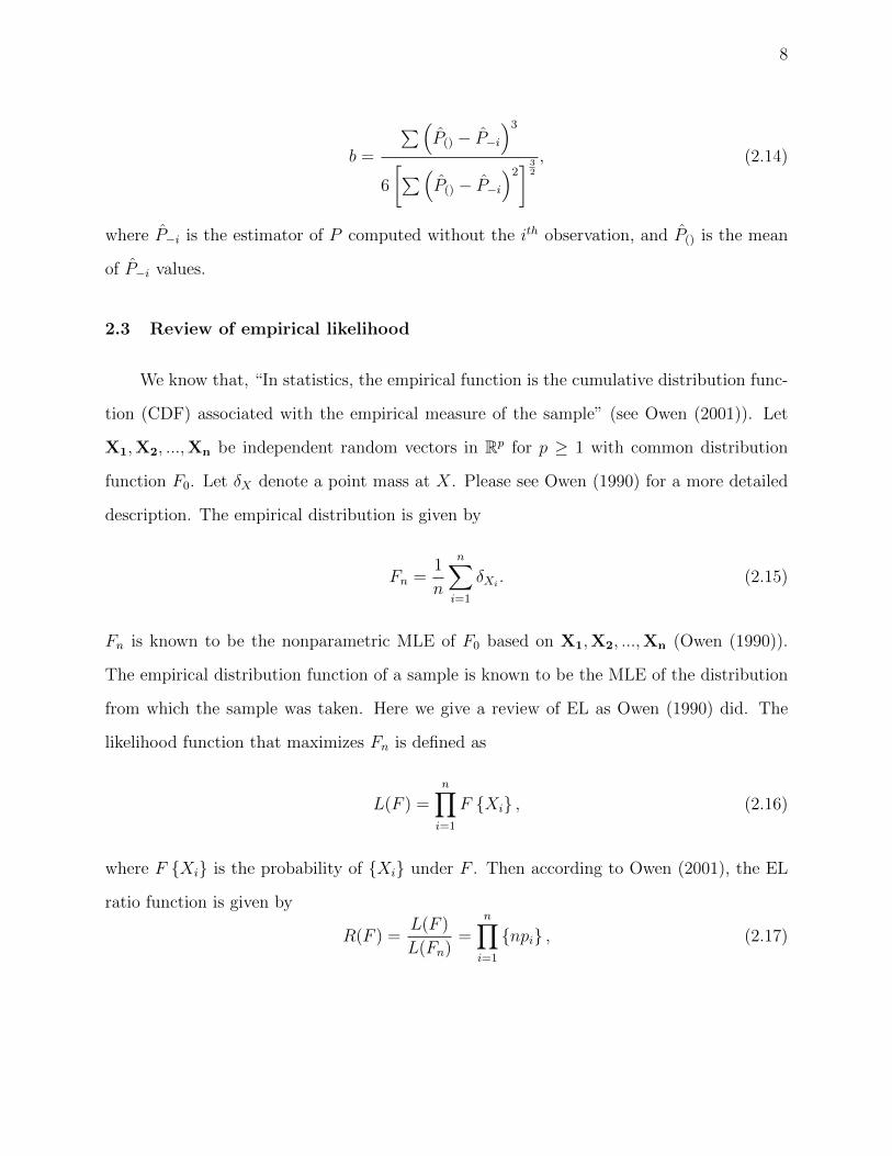
8

b =

∑(P() − P−i

)3

6

[∑(P() − P−i

)2] 3

2

, (2.14)

where P−i is the estimator of P computed without the ith observation, and P() is the mean

of P−i values.

2.3 Review of empirical likelihood

We know that, “In statistics, the empirical function is the cumulative distribution func-

tion (CDF) associated with the empirical measure of the sample” (see Owen (2001)). Let

X1,X2, ...,Xn be independent random vectors in Rp for p ≥ 1 with common distribution

function F0. Let δX denote a point mass at X. Please see Owen (1990) for a more detailed

description. The empirical distribution is given by

Fn =1

n

n∑i=1

δXi. (2.15)

Fn is known to be the nonparametric MLE of F0 based on X1,X2, ...,Xn (Owen (1990)).

The empirical distribution function of a sample is known to be the MLE of the distribution

from which the sample was taken. Here we give a review of EL as Owen (1990) did. The

likelihood function that maximizes Fn is defined as

L(F ) =n∏i=1

F {Xi} , (2.16)

where F {Xi} is the probability of {Xi} under F . Then according to Owen (2001), the EL

ratio function is given by

R(F ) =L(F )

L(Fn)=

n∏i=1

{npi} , (2.17)

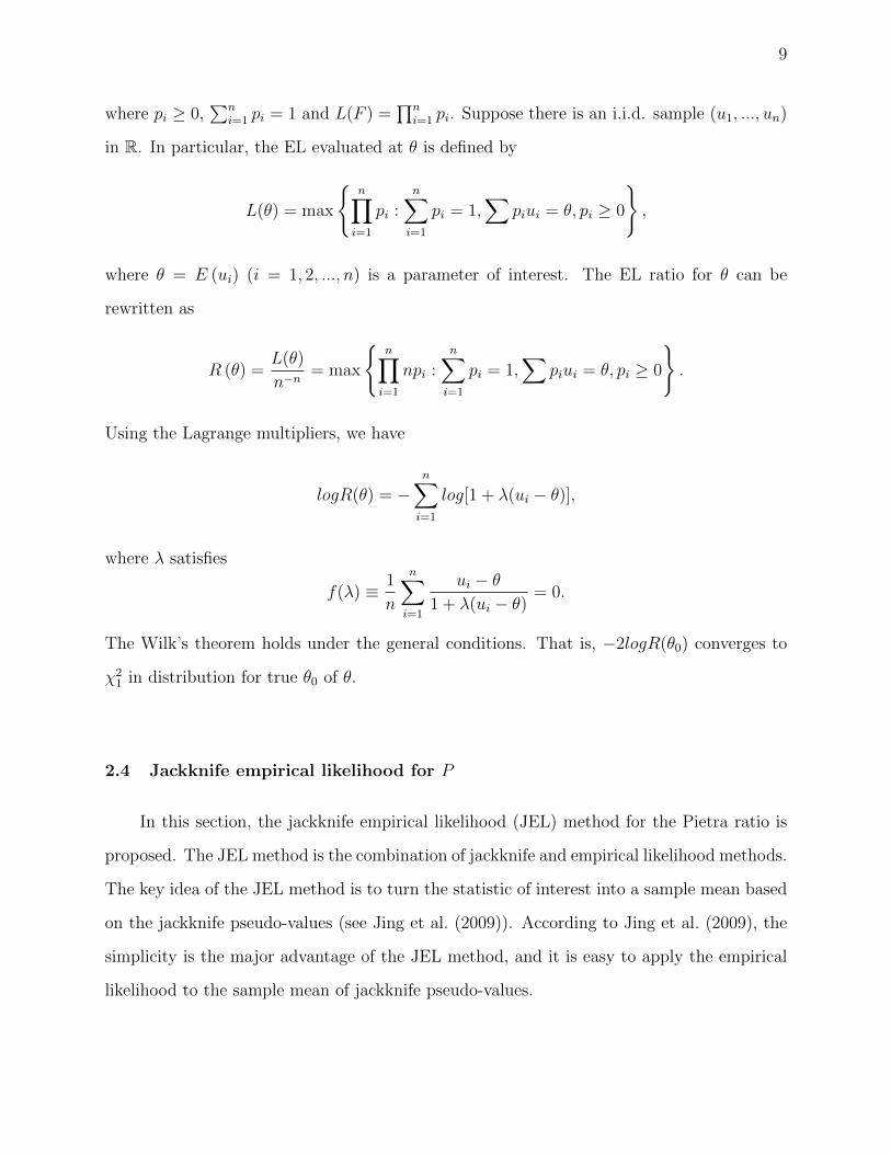
9

where pi ≥ 0,∑n

i=1 pi = 1 and L(F ) =∏n

i=1 pi. Suppose there is an i.i.d. sample (u1, ..., un)

in R. In particular, the EL evaluated at θ is defined by

L(θ) = max

{n∏i=1

pi :n∑i=1

pi = 1,∑

piui = θ, pi ≥ 0

},

where θ = E (ui) (i = 1, 2, ..., n) is a parameter of interest. The EL ratio for θ can be

rewritten as

R (θ) =L(θ)

n−n= max

{n∏i=1

npi :n∑i=1

pi = 1,∑

piui = θ, pi ≥ 0

}.

Using the Lagrange multipliers, we have

logR(θ) = −n∑i=1

log[1 + λ(ui − θ)],

where λ satisfies

f(λ) ≡ 1

n

n∑i=1

ui − θ1 + λ(ui − θ)

= 0.

The Wilk’s theorem holds under the general conditions. That is, −2logR(θ0) converges to

χ21 in distribution for true θ0 of θ.

2.4 Jackknife empirical likelihood for P

In this section, the jackknife empirical likelihood (JEL) method for the Pietra ratio is

proposed. The JEL method is the combination of jackknife and empirical likelihood methods.

The key idea of the JEL method is to turn the statistic of interest into a sample mean based

on the jackknife pseudo-values (see Jing et al. (2009)). According to Jing et al. (2009), the

simplicity is the major advantage of the JEL method, and it is easy to apply the empirical

likelihood to the sample mean of jackknife pseudo-values.

10

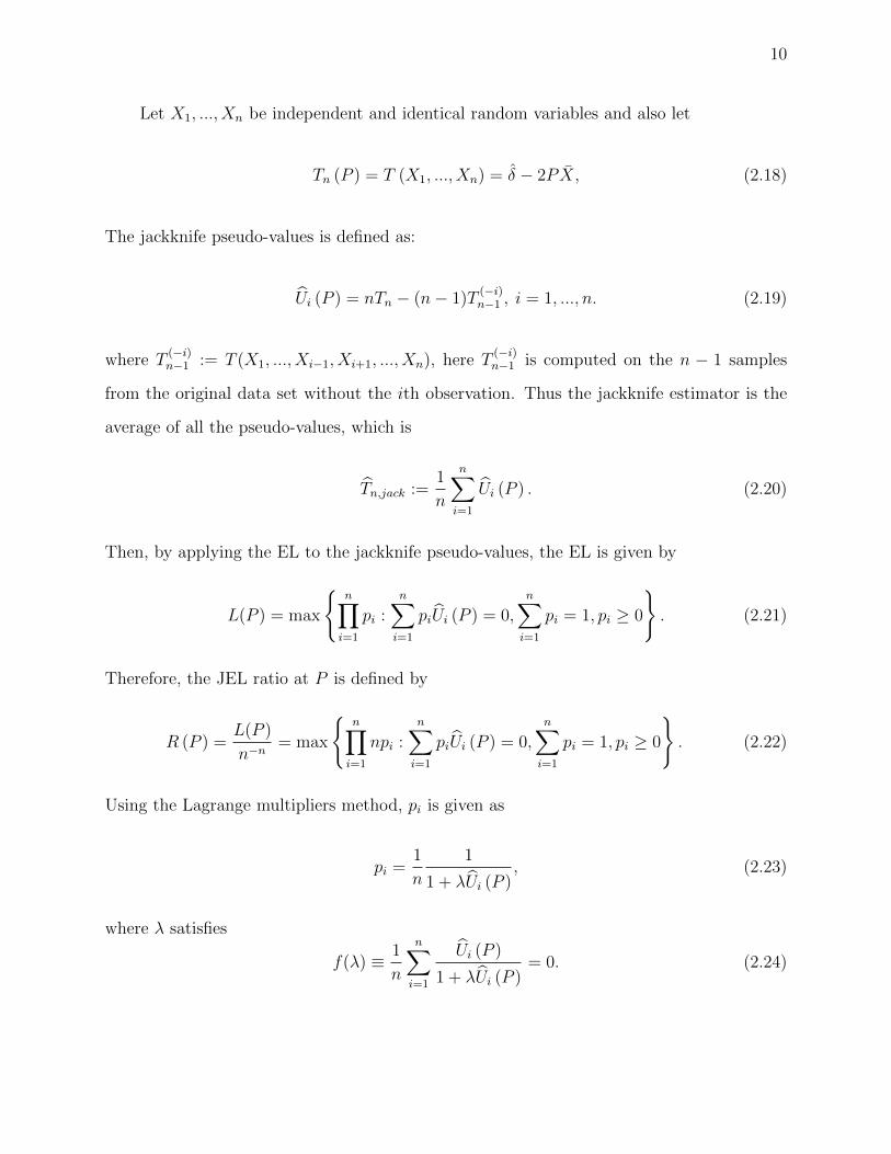
Let X1, ..., Xn be independent and identical random variables and also let

Tn (P ) = T (X1, ..., Xn) = δ − 2PX, (2.18)

The jackknife pseudo-values is defined as:

Ui (P ) = nTn − (n− 1)T(−i)n−1 , i = 1, ..., n. (2.19)

where T(−i)n−1 := T (X1, ..., Xi−1, Xi+1, ..., Xn), here T

(−i)n−1 is computed on the n − 1 samples

from the original data set without the ith observation. Thus the jackknife estimator is the

average of all the pseudo-values, which is

Tn,jack :=1

n

n∑i=1

Ui (P ) . (2.20)

Then, by applying the EL to the jackknife pseudo-values, the EL is given by

L(P ) = max

{n∏i=1

pi :n∑i=1

piUi (P ) = 0,n∑i=1

pi = 1, pi ≥ 0

}. (2.21)

Therefore, the JEL ratio at P is defined by

R (P ) =L(P )

n−n= max

{n∏i=1

npi :n∑i=1

piUi (P ) = 0,n∑i=1

pi = 1, pi ≥ 0

}. (2.22)

Using the Lagrange multipliers method, pi is given as

pi =1

n

1

1 + λUi (P ), (2.23)

where λ satisfies

f(λ) ≡ 1

n

n∑i=1

Ui (P )

1 + λUi (P )= 0. (2.24)

11

The jackknife empirical log-likelihood ratio can be derived as

logR(P ) = −n∑i=1

log{

1 + λUi (P )}. (2.25)

We display regularity conditions as Gastwirth (1974), X is a random variable with finite

mean µ and variance σ2, which has a continuous density function f(x) in the neighborhood

of µ.

Using the similar argument of Jing et al. (2009), the following Wilk’s theorem works for

the true P0 of P .

Theorem 1 Under the above regular conditions, −2logR(P0) converges to χ21 in distribution.

Using Theorem 1, the 100(1− α)% JEL confidence interval for P is constructed as follows,

R ={P : −2logR (P ) ≤ χ2

1 (α)},

where χ21 (α) is the upper α-quantile of χ2

1.

2.5 Adjusted jackknife empirical likelihood for P

In order to improve the performance of the JEL method, a novel method called adjusted

JEL is developed, which combines two nonparametric approaches: the jackknife and the

adjusted empirical likelihood. The idea of the adjusted empirical likelihood comes from Chen

et al. (2008). According to Zheng and Yu (2013), the adjustment of empirical likelihood is

better than the original empirical likelihood since it can reduce the amount of deviation.

Therefore, this idea is applied to the JEL to see whether it can perform better than the JEL

method does, and circumvent the empty set issue encountered in the classical JEL method.

The adjusted jackknife empirical likelihood (AJEL) at P is given by

L(P ) = max

{n+1∏i=1

pi :n+1∑i=1

pi = 1,n+1∑i=1

pigadi (P ) = 0, pi ≥ 0

}, (2.26)

12

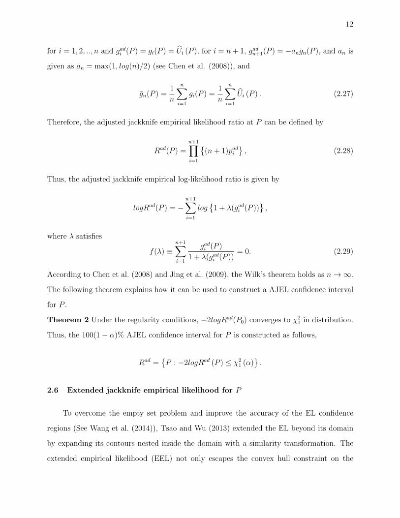
for i = 1, 2, .., n and gadi (P ) = gi(P ) = Ui (P ), for i = n+ 1, gadn+1(P ) = −angn(P ), and an is

given as an = max(1, log(n)/2) (see Chen et al. (2008)), and

gn(P ) =1

n

n∑i=1

gi(P ) =1

n

n∑i=1

Ui (P ) . (2.27)

Therefore, the adjusted jackknife empirical likelihood ratio at P can be defined by

Rad(P ) =n+1∏i=1

{(n+ 1)padi

}, (2.28)

Thus, the adjusted jackknife empirical log-likelihood ratio is given by

logRad(P ) = −n+1∑i=1

log{

1 + λ(gadi (P ))},

where λ satisfies

f(λ) ≡n+1∑i=1

gadi (P )

1 + λ(gadi (P ))= 0. (2.29)

According to Chen et al. (2008) and Jing et al. (2009), the Wilk’s theorem holds as n→∞.

The following theorem explains how it can be used to construct a AJEL confidence interval

for P .

Theorem 2 Under the regularity conditions, −2logRad(P0) converges to χ21 in distribution.

Thus, the 100(1− α)% AJEL confidence interval for P is constructed as follows,

Rad ={P : −2logRad (P ) ≤ χ2

1 (α)}.

2.6 Extended jackknife empirical likelihood for P

To overcome the empty set problem and improve the accuracy of the EL confidence

regions (See Wang et al. (2014)), Tsao and Wu (2013) extended the EL beyond its domain

by expanding its contours nested inside the domain with a similarity transformation. The

extended empirical likelihood (EEL) not only escapes the convex hull constraint on the

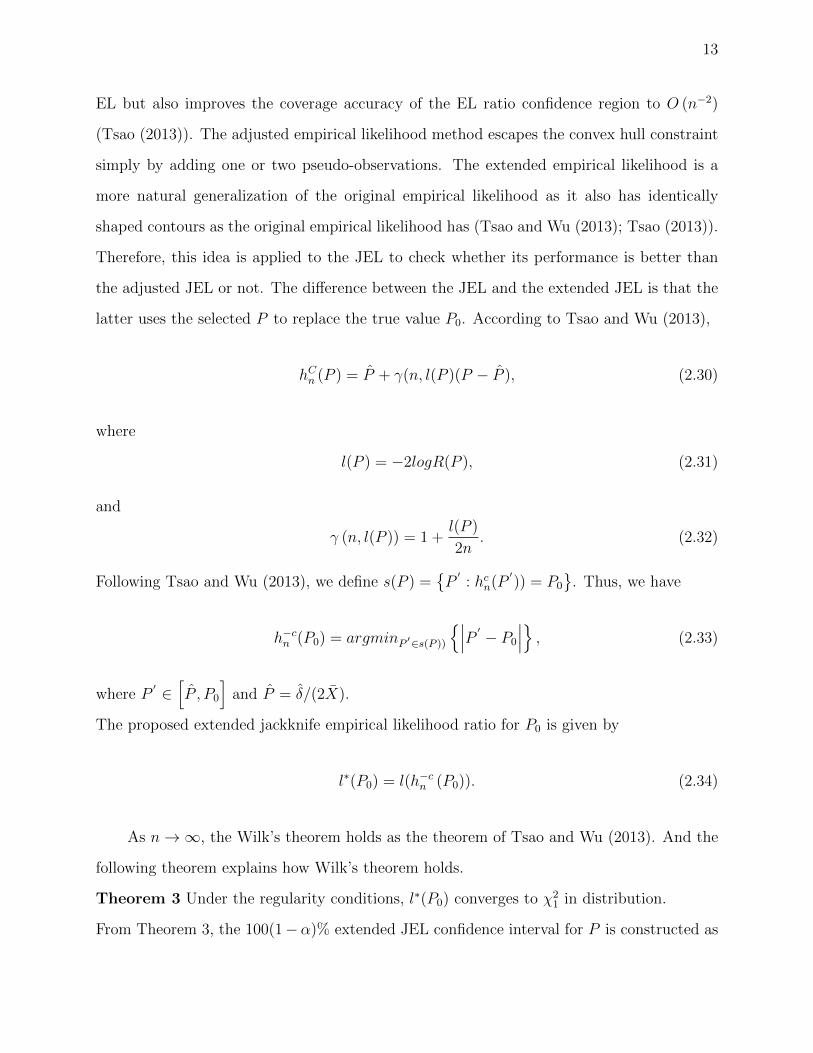
13

EL but also improves the coverage accuracy of the EL ratio confidence region to O (n−2)

(Tsao (2013)). The adjusted empirical likelihood method escapes the convex hull constraint

simply by adding one or two pseudo-observations. The extended empirical likelihood is a

more natural generalization of the original empirical likelihood as it also has identically

shaped contours as the original empirical likelihood has (Tsao and Wu (2013); Tsao (2013)).

Therefore, this idea is applied to the JEL to check whether its performance is better than

the adjusted JEL or not. The difference between the JEL and the extended JEL is that the

latter uses the selected P to replace the true value P0. According to Tsao and Wu (2013),

hCn (P ) = P + γ(n, l(P )(P − P ), (2.30)

where

l(P ) = −2logR(P ), (2.31)

and

γ (n, l(P )) = 1 +l(P )

2n. (2.32)

Following Tsao and Wu (2013), we define s(P ) ={P

′: hcn(P

′)) = P0

}. Thus, we have

h−cn (P0) = argminP ′∈s(P ))

{∣∣∣P ′ − P0

∣∣∣} , (2.33)

where P′ ∈[P , P0

]and P = δ/(2X).

The proposed extended jackknife empirical likelihood ratio for P0 is given by

l∗(P0) = l(h−cn (P0)). (2.34)

As n→∞, the Wilk’s theorem holds as the theorem of Tsao and Wu (2013). And the

following theorem explains how Wilk’s theorem holds.

Theorem 3 Under the regularity conditions, l∗(P0) converges to χ21 in distribution.

From Theorem 3, the 100(1−α)% extended JEL confidence interval for P is constructed as

14

follows,

Red ={P : l∗(P ) ≤ χ2

1 (α)}.

In the next chapter, these methods are employed to conduct an extensive simulation

study.

15

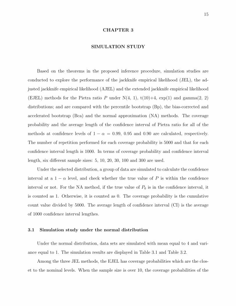
CHAPTER 3

SIMULATION STUDY

Based on the theorems in the proposed inference procedure, simulation studies are

conducted to explore the performance of the jackknife empirical likelihood (JEL), the ad-

justed jackknife empirical likelihood (AJEL) and the extended jackknife empirical likelihood

(EJEL) methods for the Pietra ratio P under N(4, 1), t(10)+4, exp(1) and gamma(2, 2)

distributions; and are compared with the percentile bootstrap (Bp), the bias-corrected and

accelerated bootstrap (Bca) and the normal approximation (NA) methods. The coverage

probability and the average length of the confidence interval of Pietra ratio for all of the

methods at confidence levels of 1 − α = 0.99, 0.95 and 0.90 are calculated, respectively.

The number of repetition performed for each coverage probability is 5000 and that for each

confidence interval length is 1000. In terms of coverage probability and confidence interval

length, six different sample sizes: 5, 10, 20, 30, 100 and 300 are used.

Under the selected distribution, a group of data are simulated to calculate the confidence

interval at a 1 − α level, and check whether the true value of P is within the confidence

interval or not. For the NA method, if the true value of P0 is in the confidence interval, it

is counted as 1. Otherwise, it is counted as 0. The coverage probability is the cumulative

count value divided by 5000. The average length of confidence interval (CI) is the average

of 1000 confidence interval lengthes.

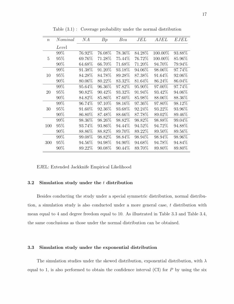
3.1 Simulation study under the normal distribution

Under the normal distribution, data sets are simulated with mean equal to 4 and vari-

ance equal to 1. The simulation results are displayed in Table 3.1 and Table 3.2.

Among the three JEL methods, the EJEL has coverage probabilities which are the clos-

et to the nominal levels. When the sample size is over 10, the coverage probabilities of the

16

AJEL are higher than those of the JEL method. The AJEL shows over coverage probabilities

when the sample size equals 5. In addition, at the level 1−α = 0.99, the coverage probability

of CI with the sample size n = 10 is higher than that with the sample size n = 20. All of

these indicate that the AJEL method is not suitable when the sample size n ≤ 10.

Among the six methods, the NA has the lowest coverage probabilities when the sample

size n ≤ 30, and the EJEL has the highest coverage probabilities when the sample size

n ≤ 10. When the sample size n equals 5, the coverage probabilities for the NA are not

satisfactory. However, the EJEL method still gives very good results. For example, at the

level 1 − α = 0.99, the coverage probability for the EJEL is 93.88% while only 76.92% for

the NA method. When the sample size is 100 or 300, the six methods give similar results.

The Bca method performs better than the Bp method.

When the sample size equals 5, the JEl method displays higher coverage probability

than the Bca method. When n = 20, the Bca is similar to the EJEL and a little bit better

than the AJEL, which has higher coverage probability than the JEL method has; and the

JEL has similar performance as Bp method. When n = 30, the Bca, AJEL and the EJEL

perform similarly.

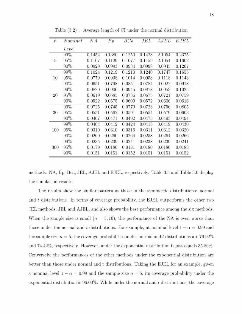
When the sample size n ≥ 10, simulation results show that the higher the coverage

probability, the longer the CI length. This pattern is in agreement with that shown by Jing

et al. (2009). The EJEL method shows the longest average lengths of CI among the six

methods, and the NA has the shortest average lengths. As the sample size increases, the CI

lengths become shorter.

Notation:

NA: Normal Approximation method

Bp: Percentile Bootstrap method

Bca: Bias Corrected and Accelerated Bootstrap method

JEL: Jackknife Empirical Likelihood

AJEL: Adjusted Jackknife Empirical Likelihood

17

Table (3.1) : Coverage probability under the normal distribution

n Nominal NA Bp Bca JEL AJEL EJEL

Level99% 76.92% 76.08% 78.36% 84.28% 100.00% 93.88%

5 95% 69.76% 71.28% 75.44% 76.72% 100.00% 85.96%90% 64.68% 66.70% 71.68% 71.20% 94.70% 79.94%99% 91.38% 91.20% 93.18% 94.06% 98.06% 97.74%

10 95% 84.28% 84.78% 89.28% 87.38% 91.64% 92.06%90% 80.06% 80.22% 83.32% 81.64% 86.24% 86.04%99% 95.64% 96.36% 97.82% 95.90% 97.00% 97.74%

20 95% 90.82% 90.42% 93.32% 91.94% 93.42% 94.06%90% 84.82% 85.86% 87.60% 85.98% 88.06% 88.36%99% 96.74% 97.10% 98.16% 97.36% 97.80% 98.12%

30 95% 91.60% 92.36% 93.68% 92.24% 93.22% 93.96%90% 86.80% 87.48% 88.66% 87.78% 89.02% 89.46%99% 98.36% 98.26% 98.82% 98.82% 98.88% 99.04%

100 95% 93.74% 93.86% 94.44% 94.52% 94.72% 94.88%90% 88.86% 88.82% 89.70% 89.22% 89.50% 89.56%99% 99.08% 98.82% 98.84% 98.94% 98.94% 98.96%

300 95% 94.56% 94.98% 94.90% 94.68% 94.78% 94.84%90% 89.22% 90.08% 90.44% 89.70% 89.80% 89.80%

EJEL: Extended Jackknife Empirical Likelihood

3.2 Simulation study under the t distribution

Besides conducting the study under a special symmetric distribution, normal distribu-

tion, a simulation study is also conducted under a more general case, t distribution with

mean equal to 4 and degree freedom equal to 10. As illustrated in Table 3.3 and Table 3.4,

the same conclusions as those under the normal distribution can be obtained.

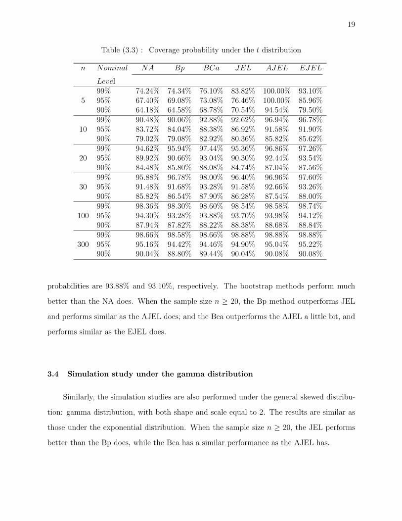
3.3 Simulation study under the exponential distribution

The simulation studies under the skewed distribution, exponential distribution, with λ

equal to 1, is also performed to obtain the confidence interval (CI) for P by using the six

18

Table (3.2) : Average length of CI under the normal distribution

n Nominal NA Bp BCa JEL AJEL EJEL

Level99% 0.1454 0.1380 0.1250 0.1428 2.1054 0.2375

5 95% 0.1107 0.1129 0.1077 0.1159 2.1054 0.160290% 0.0929 0.0993 0.0934 0.0998 0.0945 0.126799% 0.1024 0.1219 0.1210 0.1240 0.1747 0.1655

10 95% 0.0779 0.0938 0.1014 0.0958 0.1118 0.114390% 0.0651 0.0798 0.0851 0.0784 0.0922 0.091899% 0.0820 0.0906 0.0945 0.0878 0.0953 0.1025

20 95% 0.0619 0.0685 0.0736 0.0675 0.0721 0.075990% 0.0522 0.0575 0.0609 0.0572 0.0606 0.061699% 0.0725 0.0745 0.0779 0.0723 0.0756 0.0805

30 95% 0.0551 0.0562 0.0591 0.0554 0.0579 0.060390% 0.0467 0.0471 0.0492 0.0473 0.0493 0.049499% 0.0404 0.0412 0.0424 0.0415 0.0419 0.0430

100 95% 0.0310 0.0310 0.0316 0.0311 0.0312 0.032090% 0.0260 0.0260 0.0264 0.0258 0.0264 0.026699% 0.0235 0.0239 0.0241 0.0238 0.0239 0.0241

300 95% 0.0179 0.0180 0.0181 0.0180 0.0180 0.018390% 0.0151 0.0151 0.0152 0.0151 0.0151 0.0152

methods: NA, Bp, Bca, JEL, AJEL and EJEL, respectively. Table 3.5 and Table 3.6 display

the simulation results.

The results show the similar pattern as those in the symmetric distributions: normal

and t distributions. In terms of coverage probability, the EJEL outperforms the other two

JEL methods, JEL and AJEL, and also shows the best performance among the six methods.

When the sample size is small (n = 5, 10), the performance of the NA is even worse than

those under the normal and t distributions. For example, at nominal level 1− α = 0.99 and

the sample size n = 5, the coverage probabilities under normal and t distributions are 76.92%

and 74.42%, respectively. However, under the exponential distribution it just equals 35.86%.

Conversely, the performances of the other methods under the exponential distribution are

better than those under normal and t distributions. Taking the EJEL for an example, given

a nominal level 1 − α = 0.99 and the sample size n = 5, its coverage probability under the

exponential distribution is 96.00%. While under the normal and t distributions, the coverage

19

Table (3.3) : Coverage probability under the t distribution


Level99% 74.24% 74.34% 76.10% 83.82% 100.00% 93.10%

5 95% 67.40% 69.08% 73.08% 76.46% 100.00% 85.96%90% 64.18% 64.58% 68.78% 70.54% 94.54% 79.50%99% 90.48% 90.06% 92.88% 92.62% 96.94% 96.78%

10 95% 83.72% 84.04% 88.38% 86.92% 91.58% 91.90%90% 79.02% 79.08% 82.92% 80.36% 85.82% 85.62%99% 94.62% 95.94% 97.44% 95.36% 96.86% 97.26%

20 95% 89.92% 90.66% 93.04% 90.30% 92.44% 93.54%90% 84.48% 85.80% 88.08% 84.74% 87.04% 87.56%99% 95.88% 96.78% 98.00% 96.40% 96.96% 97.60%

30 95% 91.48% 91.68% 93.28% 91.58% 92.66% 93.26%90% 85.82% 86.54% 87.90% 86.28% 87.54% 88.00%99% 98.36% 98.30% 98.60% 98.54% 98.58% 98.74%

100 95% 94.30% 93.28% 93.88% 93.70% 93.98% 94.12%90% 87.94% 87.82% 88.22% 88.38% 88.68% 88.84%99% 98.66% 98.58% 98.66% 98.88% 98.88% 98.88%

300 95% 95.16% 94.42% 94.46% 94.90% 95.04% 95.22%90% 90.04% 88.80% 89.44% 90.04% 90.08% 90.08%

probabilities are 93.88% and 93.10%, respectively. The bootstrap methods perform much

better than the NA does. When the sample size n ≥ 20, the Bp method outperforms JEL

and performs similar as the AJEL does; and the Bca outperforms the AJEL a little bit, and

performs similar as the EJEL does.

3.4 Simulation study under the gamma distribution

Similarly, the simulation studies are also performed under the general skewed distribu-

tion: gamma distribution, with both shape and scale equal to 2. The results are similar as

those under the exponential distribution. When the sample size n ≥ 20, the JEL performs

better than the Bp does, while the Bca has a similar performance as the AJEL has.

20

Table (3.4) : Average length of CI under the t distribution


Level99% 0.1671 0.1889 0.5358 0.1635 2.1221 0.2757

5 95% 0.1271 0.1361 0.1436 0.1337 2.1216 0.185590% 0.1067 0.1170 0.1173 0.1154 0.1187 0.143199% 0.1371 0.1435 0.1464 0.1448 0.1883 0.1937

10 95% 0.1067 0.1097 0.1240 0.1109 0.1306 0.133490% 0.0888 0.0938 0.1035 0.0931 0.1075 0.107199% 0.1037 0.1079 0.1151 0.0969 0.1059 0.1131

20 95% 0.0791 0.0815 0.0908 0.0767 0.0820 0.085090% 0.0650 0.0684 0.0743 0.0645 0.0686 0.069499% 0.0855 0.0872 0.0929 0.0810 0.0848 0.0903

30 95% 0.0649 0.0659 0.0707 0.0625 0.0651 0.066990% 0.0550 0.0552 0.0584 0.0539 0.0561 0.056899% 0.0478 0.0487 0.0507 0.0471 0.0478 0.0493

100 95% 0.0365 0.0367 0.0377 0.0361 0.0366 0.037490% 0.0307 0.0308 0.0314 0.0298 0.0304 0.031399% 0.0278 0.0282 0.0287 0.0280 0.0284 0.0286

300 95% 0.0211 0.0213 0.0215 0.0206 0.0207 0.021790% 0.0178 0.0179 0.0180 0.0173 0.0173 0.0178

3.5 Conclusion

First of all, as the sample size n increases, all the six methods improve their perfor-

mance in terms of coverage probabilities and average lengths of confidence intervals. When

the sample size is big enough (n = 100, 300), all the six methods have a similar performance.

Secondly, among the six methods, the EJEL has the best performance and the NA has the

worst performance. The difference in the performance between the EJEL and the other

methods is even more obvious when the sample size is small. The EJEL performs well even

when the sample size only equals 5. Under skewed distributions, the performances of the NA

are even worse than those of symmetric distributions. However, all the other methods have

better performances under skewed distributions. Third, among the three JEL methods, the

EJEL is the best one, and the AJEL is better than the JEL when the sample size is bigger

than 10. When the sample size equals 5 and 10, the AJEL shows over coverage probability

21

Table (3.5) : Coverage probability under the exponential distribution


Level99% 35.86% 83.26% 85.20% 88.10% 100.00% 96.00%

5 95% 28.52% 79.04% 82.20% 83.14% 100.00% 90.02%90% 24.32% 73.56% 77.66% 76.98% 97.26% 84.84%99% 76.44% 94.56% 96.50% 95.06% 98.82% 98.68%

10 95% 69.92% 88.88% 92.24% 88.80% 92.70% 92.46%90% 63.64% 84.14% 86.42% 83.20% 87.58% 87.26%99% 93.70% 98.22% 98.66% 97.56% 98.14% 98.90%

20 95% 85.98% 93.08% 93.94% 91.76% 93.36% 94.44%90% 80.80% 87.64% 88.14% 85.72% 88.06% 89.08%99% 96.20% 98.24% 98.68% 97.78% 98.14% 98.68%

30 95% 90.94% 93.10% 93.96% 92.70% 93.76% 94.60%90% 83.66% 87.64% 88.16% 87.04% 88.24% 89.18%99% 98.60% 98.72% 98.82% 98.32% 98.58% 98.70%

100 95% 93.96% 94.62% 94.60% 94.20% 94.46% 94.84%90% 88.16% 89.52% 89.78% 89.02% 89.28% 90.24%99% 98.80% 98.88% 98.82% 98.76% 98.78% 98.80%

300 95% 94.38% 95.10% 95.08% 94.62% 94.70% 95.08%90% 90.28% 90.16% 90.08% 89.10% 89.22% 89.62%

of CI. Fourth, the Bca performs better than the Bp and NA do. Under the symmetric dis-

tribution, the Bp performs similar as the NA does. However, under the skewed distribution,

the Bp has a much better performance than the NA has. When n ≥ 20, the Bca outperforms

the JEL and Bp, and has a similar performance as the AJEL method has. However, when

the sample size n = 5, the JEL outperforms the Bca and the Bp methods. Finally, the

computation time of JEL methods is much shorter than that of the two bootstrap methods,

and the JEL and AJEL are much faster than the EJEL method.

22

Table (3.6) : Average length of CI under the exponential distribution


Level99% 0.3772 0.4838 0.4439 0.4396 2.3465 0.7522

5 95% 0.2870 0.3882 0.3676 0.3644 2.3399 0.479490% 0.2409 0.3353 0.3140 0.3176 0.4588 0.371399% 0.2851 0.3798 0.3700 0.3762 0.3548 0.4918

10 95% 0.2169 0.2903 0.2907 0.2947 0.3429 0.351390% 0.1820 0.2442 0.2430 0.2503 0.3426 0.283799% 0.2345 0.2764 0.2779 0.2785 0.2961 0.3333

20 95% 0.1784 0.2096 0.2114 0.2116 0.2239 0.236790% 0.1498 0.1760 0.1769 0.1779 0.1893 0.193299% 0.2052 0.2283 0.2308 0.2272 0.2361 0.2540

30 95% 0.1547 0.1732 0.1748 0.1727 0.1797 0.184290% 0.1292 0.1454 0.1465 0.1446 0.1502 0.151899% 0.1215 0.1260 0.1270 0.1248 0.1263 0.1289

100 95% 0.0926 0.0952 0.0957 0.0947 0.0958 0.097190% 0.0775 0.0798 0.0803 0.0795 0.0802 0.080699% 0.0717 0.0731 0.0735 0.0725 0.0727 0.0733

300 95% 0.0545 0.0552 0.0554 0.0550 0.0553 0.055890% 0.0457 0.0463 0.0464 0.0463 0.0464 0.0463

23

Table (3.7) : Coverage probability under the gamma distribution


Level99% 48.62% 79.94% 82.24% 84.02% 100.0% 94.58%

5 95% 42.36% 75.08% 80.12% 76.04% 100.0% 86.88%90% 38.30% 70.12% 74.88% 69.90% 96.3% 80.18%99% 86.22% 93.94% 96.34% 95.28% 98.6% 98.44%

10 95% 78.12% 89.14% 91.74% 88.56% 92.7% 93.26%90% 71.64% 83.82% 86.52% 82.62% 87.2% 87.06%99% 94.96% 96.66% 98.14% 97.42% 98.3% 98.96%

20 95% 88.72% 91.22% 93.60% 92.74% 94.2% 94.88%90% 82.40% 86.46% 87.80% 87.36% 89.2% 89.42%99% 96.80% 97.72% 98.60% 98.12% 98.5% 98.90%

30 95% 91.36% 92.88% 94.16% 93.80% 94.5% 95.16%90% 86.32% 87.90% 88.56% 86.80% 88.1% 88.40%99% 98.52% 98.60% 98.90% 0.9854 98.7% 98.84%

100 95% 93.56% 93.68% 94.12% 0.9448 94.7% 94.90%90% 88.94% 89.08% 89.00% 0.8966 90.1% 90.12%99% 98.78% 99.24% 99.18% 0.9902 99.0% 99.10%

300 95% 95.36% 95.34% 95.34% 0.9494 95.0% 95.06%90% 89.92% 90.36% 90.38% 0.8988 89.9% 89.94%

24

Table (3.8) : Average length of CI under the gamma distribution


Level99% 0.3107 0.3590 0.3281 0.3346 2.2679 0.5750

5 95% 0.2364 0.2921 0.2766 0.2785 2.2625 0.351190% 0.1984 0.2523 0.2387 0.2401 0.2458 0.280099% 0.2436 0.2908 0.2848 0.2976 0.4133 0.3935

10 95% 0.1854 0.2224 0.2279 0.2314 0.2704 0.276690% 0.1556 0.1871 0.1907 0.1954 0.2232 0.222599% 0.1954 0.2167 0.2206 0.2149 0.2306 0.2517

20 95% 0.1492 0.1646 0.1687 0.1643 0.1752 0.180490% 0.1242 0.1382 0.1412 0.1378 0.1458 0.147699% 0.1668 0.1777 0.1821 0.1741 0.1821 0.1937

30 95% 0.1268 0.1347 0.1372 0.1343 0.1397 0.143490% 0.1066 0.1132 0.1147 0.1132 0.1174 0.118399% 0.0960 0.0986 0.1000 0.0972 0.0982 0.1003

100 95% 0.0736 0.0746 0.0752 0.0739 0.0748 0.075990% 0.0615 0.0626 0.0630 0.0622 0.0629 0.063599% 0.0564 0.0571 0.0574 0.0567 0.0568 0.0573

300 95% 0.0428 0.0430 0.0431 0.0431 0.0432 0.043790% 0.0359 0.0361 0.0362 0.0360 0.0361 0.0362

25

CHAPTER 4

REAL DATA ANALYSIS

In this part, the real data sets with small, moderate and large sample sizes are used to

illustrate the proposed methods. The NA, Bp, Bca, JEL, AJEL and EJEL methods are ap-

plied to the three real data sets. Their confidence interval length and the confidence interval

bounds of point estimate of the Pietra ratio P at three nominal levels: 1 − α =0.99, 0.95

and 0.90 are calculated.

The first data set “airmiles”, which comes from R data package “datasets”, has 24 ob-

servations. The second data set “white income” obtained from the U.S. Census Bureau web

site has 41 observations. The third data set ”housefly wing” has 100 observations, selected

from Biometry (Sokal and Rohlf (1968)).

The Shapiro-Wilk test is used to check the normality of the three real data sets. The null

hypothesis of the Shapiro-Wilk test is that the sample data follows the normal distribution.

If the p−value of the Shapiro-Wilk test is higher than 0.05, the null hypothesis will not be

rejected, and the confidence interval (CI) lengths of the real data sets will be compared with

those in the simulation study under normal distribution. Otherwise, the goodness-of-fit test

for the exponential distribution based on the Gini Statistic (see Gail and Gastwirth (1978))

will be used. The null hypothesis of the test is that the data follows exponential distribution.

If the p-value of the test higher than 0.05, the null hypothesis will not be rejected, and we

assume the data follow exponential distribution. And the CI lengths of the real data sets will

be compared with those under exponential or gamma distributions. The histogram of the

three real data sets are also drawn to double check whether they follow a normal distribution.

26

4.1 Airmiles data analysis

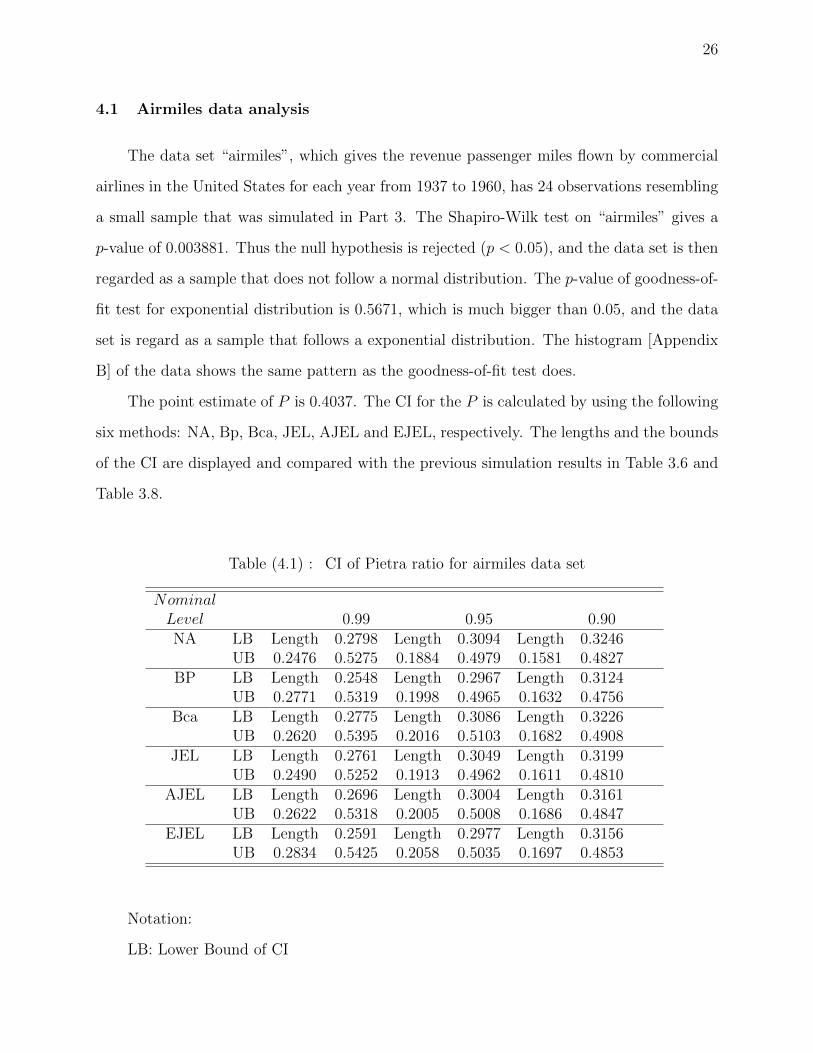
The data set “airmiles”, which gives the revenue passenger miles flown by commercial

airlines in the United States for each year from 1937 to 1960, has 24 observations resembling

a small sample that was simulated in Part 3. The Shapiro-Wilk test on “airmiles” gives a

p-value of 0.003881. Thus the null hypothesis is rejected (p < 0.05), and the data set is then

regarded as a sample that does not follow a normal distribution. The p-value of goodness-of-

fit test for exponential distribution is 0.5671, which is much bigger than 0.05, and the data

set is regard as a sample that follows a exponential distribution. The histogram [Appendix

B] of the data shows the same pattern as the goodness-of-fit test does.

The point estimate of P is 0.4037. The CI for the P is calculated by using the following

six methods: NA, Bp, Bca, JEL, AJEL and EJEL, respectively. The lengths and the bounds

of the CI are displayed and compared with the previous simulation results in Table 3.6 and

Table 3.8.

Table (4.1) : CI of Pietra ratio for airmiles data set

NominalLevel 0.99 0.95 0.90NA LB Length 0.2798 Length 0.3094 Length 0.3246

UB 0.2476 0.5275 0.1884 0.4979 0.1581 0.4827BP LB Length 0.2548 Length 0.2967 Length 0.3124

UB 0.2771 0.5319 0.1998 0.4965 0.1632 0.4756Bca LB Length 0.2775 Length 0.3086 Length 0.3226

UB 0.2620 0.5395 0.2016 0.5103 0.1682 0.4908JEL LB Length 0.2761 Length 0.3049 Length 0.3199

UB 0.2490 0.5252 0.1913 0.4962 0.1611 0.4810AJEL LB Length 0.2696 Length 0.3004 Length 0.3161

UB 0.2622 0.5318 0.2005 0.5008 0.1686 0.4847EJEL LB Length 0.2591 Length 0.2977 Length 0.3156

UB 0.2834 0.5425 0.2058 0.5035 0.1697 0.4853

Notation:

LB: Lower Bound of CI

27

UB: Upper Bound of CI

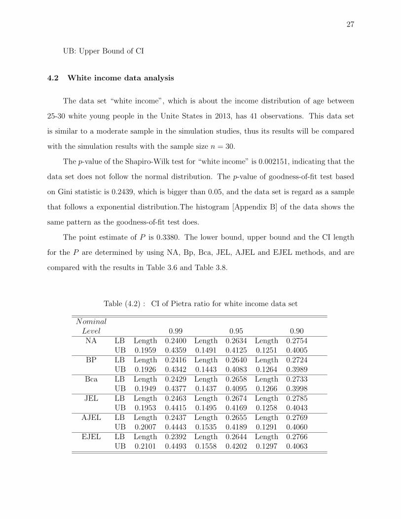
4.2 White income data analysis

The data set “white income”, which is about the income distribution of age between

25-30 white young people in the Unite States in 2013, has 41 observations. This data set

is similar to a moderate sample in the simulation studies, thus its results will be compared

with the simulation results with the sample size n = 30.

The p-value of the Shapiro-Wilk test for “white income” is 0.002151, indicating that the

data set does not follow the normal distribution. The p-value of goodness-of-fit test based

on Gini statistic is 0.2439, which is bigger than 0.05, and the data set is regard as a sample

that follows a exponential distribution.The histogram [Appendix B] of the data shows the

same pattern as the goodness-of-fit test does.

The point estimate of P is 0.3380. The lower bound, upper bound and the CI length

for the P are determined by using NA, Bp, Bca, JEL, AJEL and EJEL methods, and are

compared with the results in Table 3.6 and Table 3.8.

Table (4.2) : CI of Pietra ratio for white income data set







UB 0.2101 0.4493 0.1558 0.4202 0.1297 0.4063

28

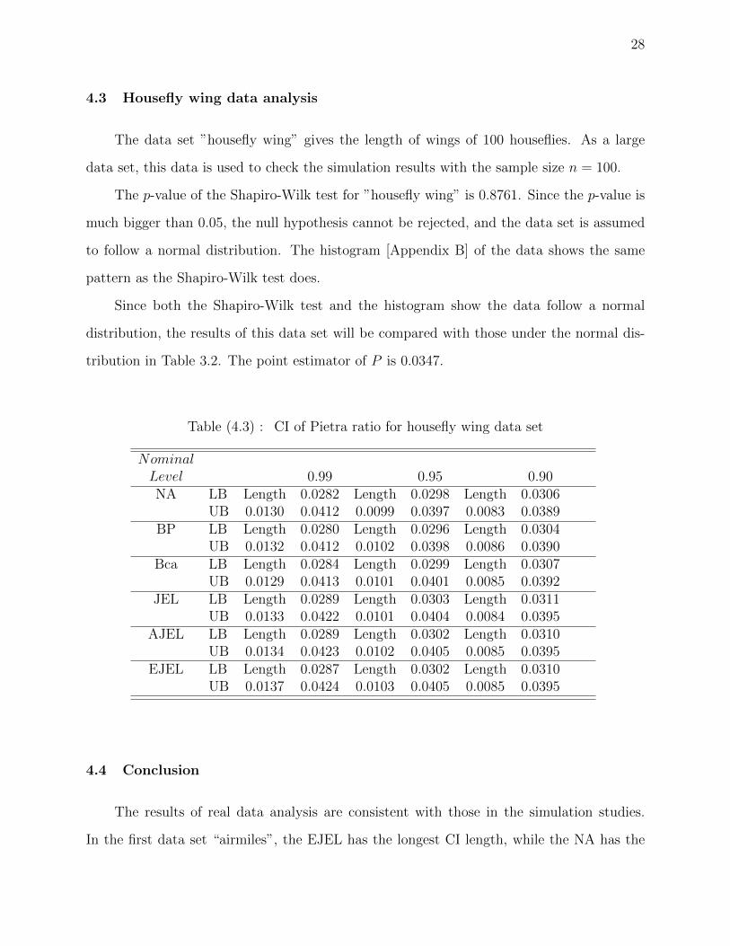
4.3 Housefly wing data analysis

The data set ”housefly wing” gives the length of wings of 100 houseflies. As a large

data set, this data is used to check the simulation results with the sample size n = 100.

The p-value of the Shapiro-Wilk test for ”housefly wing” is 0.8761. Since the p-value is

much bigger than 0.05, the null hypothesis cannot be rejected, and the data set is assumed

to follow a normal distribution. The histogram [Appendix B] of the data shows the same

pattern as the Shapiro-Wilk test does.

Since both the Shapiro-Wilk test and the histogram show the data follow a normal

distribution, the results of this data set will be compared with those under the normal dis-

tribution in Table 3.2. The point estimator of P is 0.0347.

Table (4.3) : CI of Pietra ratio for housefly wing data set







UB 0.0137 0.0424 0.0103 0.0405 0.0085 0.0395

4.4 Conclusion

The results of real data analysis are consistent with those in the simulation studies.

In the first data set “airmiles”, the EJEL has the longest CI length, while the NA has the

29

shortest one, and the CI lengths for Bp, Bca and AJEL are longer than that for the JEL.

The results are in agreement with the results in Table 3.8 when the sample size n equals 20.

In the data set “white income”, the CI lengths for the EJEL is longer than those for the

other methods, and the CI lengths for the other methods are similar, which agree with those

having the sample size n = 30 in Table 3.6 and Table 3.8. As for the third data set “housefly

wing”, the CI lengths under all the six methods are similar, which are also consistent with

previous simulation studies under a normal distribution when the sample size n equals 100.

The CIs of P for all of the three real datas are symmetric for the NA method. However,

the CIs are asymmetric when using the other methods, especially when using the EJEL

method. The CIs of the skewed data sets “airmiles” and “white income” are more asym-

metric than those of the approximate symmetric data set “housefly wing” under the two

bootstrap methods and the three JEL methods.

30

CHAPTER 5

SUMMARY AND FUTURE WORK

5.1 Summary

In this thesis, different interval estimators of Pietra ratio P are developed by using the

NA, Bp, BCa, JEL, AJEL and EJEL methods. As illustrated by the simulation studies,

the JEL methods exhibit two advantages over the other methods. The first one is that the

JEL methods can give a better coverage probability of the confidence interval than the NA

method does when the sample size is small. Secondly, although the bootstrap methods Bp

and Bca can also give good performances when the sample size is bigger than 5, the compu-

tational time of the JEL methods is much shorter.

When the sample size is very small (n < 20), the EJEL gives the best performance.

However, if the sample size is bigger than 20, the JEL or the AJEL method will be the wise

choice since they can not only produce a comparable result as the EJEL method can, but

also take much less computation time than the latter does.

5.2 Future Work

Previous papers (Jing et al. (2009); Chen et al. (2008); Zheng and Yu (2013); Tsao

and Wu (2013); Tsao (2013)) showed that the JEL, AEL and EEL methods have advan-

tages over other methods when dealing with multi-dimensional data. Our current studies

indicated that the AJEL and EJEL methods outperform the other methods. However, all

of the data used in these studies are one dimensional. Therefore, in the future, our work

will be focused on whether the AJEL and EJEL methods also show better performance on

multi-dimensional frame work. We will extend the proposed JEL methods for the Pietra

ratio with missing at random or right censoring data. In addition, we would like to make an

31

JEL inference for the difference of two Pietra ratio. In the future, we would like to discuss

the more robust definition of the Pietra ratio by replacing the denominator with two times

medium of a population. It is a challenge for us to develop nonparametric methods for the

new Pietra ratio.

32

REFERENCES

Adimari, G. and Chiogna, M. (2012). Jackknife empirical likelihood based confidence inter-

vals for partial areas under ROC curves. Statistica Sinica, 22:1457–1477.

Bouadoumou, M., Zhao, Y., and Lu, Y. (2014). Jackknife empirical likelihood for the accel-

erated failure time model with censored data. Communications in Statistics - Simulation

and Computation. to appear.

Carpenter, J. and Bithell, J. (2000). Bootstrap confidence intervals: when, which, what? a

practical guide for medical statisticians. Statistics in medicine, 19(9)(24):1141–1164.

Chen, J. and Liu, Y. (2012). Adjusted empirical likelihood with high-order one-sided coverage

precision. Statistics and Its Interface, 5:281–292.

Chen, J., Variyath, A., and Abraham, B. (2008). Adjusted empirical likelihood and its

properties. J Comput Graph Stat, 17:426–443.

Chen, S. X. and Cui, H. (2007). On the second-order properties of empirical likelihood with

moment restrictions. Journal of Econometrics, 141:492–516.

Chen, S. X. and Keilegom, I. V. (2009). A review on empirical likelihood methods for

regression. Test, 18(33):415–447.

Efron, B. (1987). Better bootstrap confidence intervals. Journal of the American Statistical

Association, 82(397)(15):171–185.

Eliazar, I. I. and Sokolov, I. M. (2010). Measuring statistical heterogeneity: The Pietra

index. Physica A, 389:117–125.

Gail, M. H. and Gastwirth, J. L. (1978). A scale-free goodness-of-fit test for the exponential

distribution based on the Gini statistic. J. R. Statist. Soc. B, 3:350–357.

33

Gastwirth, J. L. (1974). Large sample theory of some measures of income inequality. Econo-

metrica, 42:191–196.

Gong, Y., Peng, L., and Qi, Y. (2010). Smoothed jackknife empirical likelihood method for

ROC curve. Journal of Multivariate Analysis, 101:1520–1531.

Habib, E. A. (2012). On the decomposition of the schutz coefficient: an exact approach with

an application. Electron. J. App. Stat. Anal., 5:187–198.

Jing, B.-Y., Yuan, J., and Zhou, W. (2009). Jackknife empirical likelihood. Journal of the

American Statistical Association, 104(487):1224–1232.

Kendall, J. L. and Stuart, A. (1963). The Advanced Theory of Statistics, volume 2nd ed.

London:Griffen.

Kennedy, B. P., Kawachi, I., and Prothrow-Stith, D. (1996). Income distribution and mortal-

ity: cross sectional ecological study of the Robin Hood index in the United States. BMJ,

312:1004–1007.

Liu, Y. and Chen, J. (2010). Adjusted empirical likelihood with high-order precision. The

Annals of Statistics, 38:1341–1362.

Maio, F. G. D. (2007). Income inequality measures. J Epidemiol Community Health,

61(10):849–852.

Owen, A. B. (1988). Empirical likelihood ratio confidence intervals for a single functional.

Biometrika, 75(2):237–249.

Owen, A. B. (1990). Empirical likelihood ratio confidence regions. The Annals of Statistics,

18(1):90–120.

Owen, A. B. (2001). Empirical Likelihood. Chapman Hall/CRC.

Quenouille, M. (1956). Notes on bias in estimation. Biometrika, 10:353–360.

34

Salverda, W., Nolan, B., and Smeeding, T. M. (2009). The Oxford handbook of economic

inequality. Business Economics, page 51.

Schutz, R. R. (1951). On the measurement of income inequality. The American Economic

Review, 41:107–122.

Shi, L., Macinko, J., Starfield, B., Wulu, J., Regan, J., and Politzer, R. (2003). The rela-

tionship between primary care, income inequality, and mortality in US States 1980-1995.

J Am Board Fam Med, 16:412–422.

Sohler, N. L., Arno, P. S., Chang, C. J., Fang, J., and Schechter, C. (2003). Income inequality

and infant mortality in New York City. J Urban Health, 80:650–657.

Sokal, R. and Rohlf, F. (1968). Biometry. Freeman Publishing Co.

Tsao, M. (2013). Extending the empirical likelihood by domain expansion. The Canadian

Journal of Statistics, 41(2):257–274.

Tsao, M. and Wu, F. (2013). Extended empirical likelihood for estimating equations. vol-

ume 99, pages 1–14.

Wang, H. and Zhao, Y. (2009). A comparison of some confidence intervals for the mean

quality-adjusted lifetime with censored data. Computational Statistics and Data Analysis,

53:2733–2739.

Wang, L., Chen, J., and Pu, X. (2014). Resampling calibrated adjusted empirical likelihood.

The Canadian Journal of Statistics, xx:1–18.

Wang, R., Peng, L., and Qi, Y. (2013). Jackknife empirical likelihood test for equality of

two high dimensional means. Statistica Sinica, 23:667–690.

Yang, H. and Zhao, Y. (2013). Smoothed jackknife empirical likelihood inference for the

difference of ROC curves. Journal of Multivariate Analysis, 115:270–284.

35

Zheng, M. and Yu, W. (2013). Empirical likelihood method for multivariate Cox regression.

Comput Stat, 28:1241–1267.

36

Appendix A

ROBIN HOOD INDEX

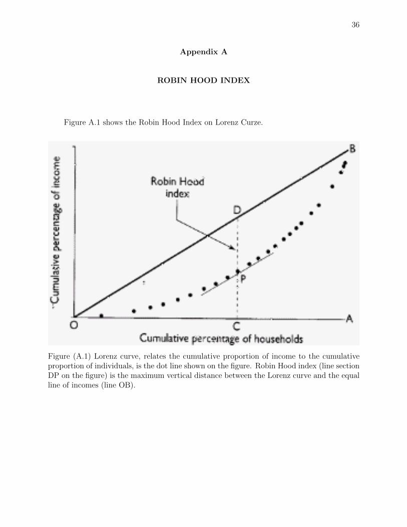
Figure A.1 shows the Robin Hood Index on Lorenz Curze.

Figure (A.1) Lorenz curve, relates the cumulative proportion of income to the cumulativeproportion of individuals, is the dot line shown on the figure. Robin Hood index (line sectionDP on the figure) is the maximum vertical distance between the Lorenz curve and the equalline of incomes (line OB).

37

Appendix B

THE HISTOGRAMS OF REAL DATA SETS

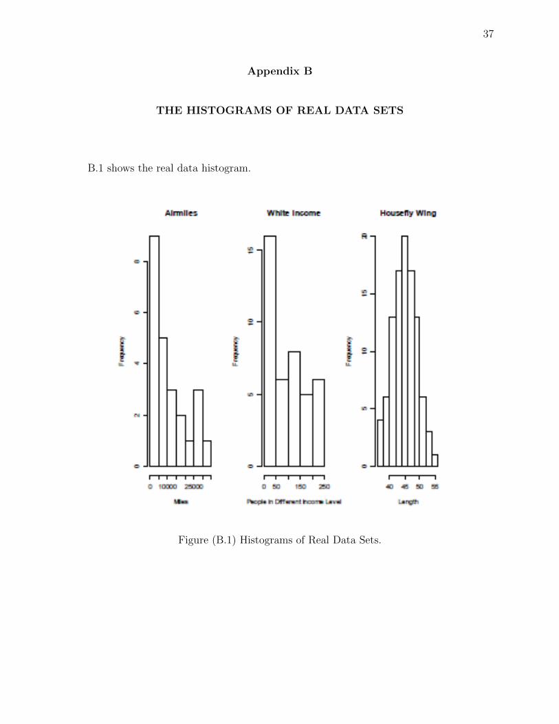
B.1 shows the real data histogram.

Figure (B.1) Histograms of Real Data Sets.

Documents

Jackknife Empirical Likelihood Inference For The … EMPIRICAL LIKELIHOOD INFERENCE FOR THE PIETRA RATIO by YUEJU SU Under the Direction of Yichuan Zhao, PhD ABSTRACT Pietra ratio