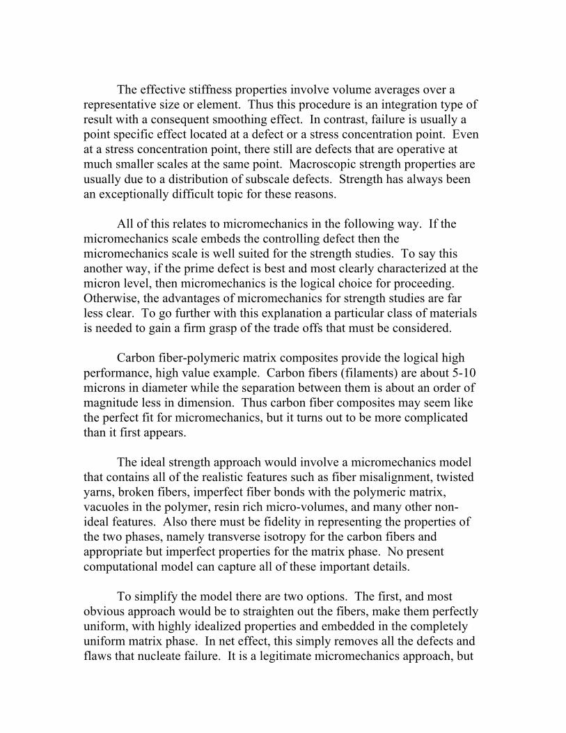
IX. MICROMECHANICS FAILURE ANALYSIS Taken literally, micromechanics refers to mechanics of materials effects at the 10-6 m scale. Usually however the term is used more broadly as representing effects at scales somewhat larger the nano-scale size but much smaller than the macroscopic size. They may center on the micron scale but they can also reach up and down considerably from that size. Micromechanics certainly offers an appealing look at basic effects at intermediate length scales. Many of the problems of special interest in the micromechanics domain are related to inclusions that are dispersed into an otherwise continuous phase. Doing this mixing at or near the micron scale affords an enormous variety of materials combinations that can yield a huge array of enhanced properties. When done properly, the combinations can achieve the best attributes of the constituents. When done casually or carelessly it almost always degenerates to the worst from each or all. The properties that are to be improved include stiffness, strength, toughness, processability, stability, durability and a host of other, sometime specialized properties. Of particular interest here are the cases of improving or optimizing stiffness and strength. Stiffness will immediately and briefly be considered and then strength will occupy the major effort in this section. There are many books and countless papers focused upon micromechanics. The vast majority of these deal with the effective stiffness properties. The field of composite materials is the recognized marketplace for such works. For example, the book “Mechanics of Composite Materials”, Christensen [1], is largely given over to the micromechanics analysis of particulate and fibrous reinforcement of a continuous matrix phase. The objective in most books is to determine the effective stiffness properties of the composite material in terms of the corresponding properties of the phases. There is a very good reason why the effort has been mainly devoted to effective stiffness properties. These stiffness type problems can be and are carefully posed so as to be amenable to complete mechanics type analysis. The micromechanics situation with strength is much more difficult. This requires some explanation.

The effective stiffness properties involve volume averages over a representative size or element. Thus this procedure is an integration type of result with a consequent smoothing effect. In contrast, failure is usually a point specific effect located at a defect or a stress concentration point. Even at a stress concentration point, there still are defects that are operative at much smaller scales at the same point. Macroscopic strength properties are usually due to a distribution of subscale defects. Strength has always been an exceptionally difficult topic for these reasons. All of this relates to micromechanics in the following way. If the micromechanics scale embeds the controlling defect then the micromechanics scale is well suited for the strength studies. To say this another way, if the prime defect is best and most clearly characterized at the micron level, then micromechanics is the logical choice for proceeding. Otherwise, the advantages of micromechanics for strength studies are far less clear. To go further with this explanation a particular class of materials is needed to gain a firm grasp of the trade offs that must be considered. Carbon fiber-polymeric matrix composites provide the logical high performance, high value example. Carbon fibers (filaments) are about 5-10 microns in diameter while the separation between them is about an order of magnitude less in dimension. Thus carbon fiber composites may seem like the perfect fit for micromechanics, but it turns out to be more complicated than it first appears. The ideal strength approach would involve a micromechanics model that contains all of the realistic features such as fiber misalignment, twisted yarns, broken fibers, imperfect fiber bonds with the polymeric matrix, vacuoles in the polymer, resin rich micro-volumes, and many other non-ideal features. Also there must be fidelity in representing the properties of the two phases, namely transverse isotropy for the carbon fibers and appropriate but imperfect properties for the matrix phase. No present computational model can capture all of these important details. To simplify the model there are two options. The first, and most obvious approach would be to straighten out the fibers, make them perfectly uniform, with highly idealized properties and embedded in the completely uniform matrix phase. In net effect, this simply removes all the defects and flaws that nucleate failure. It is a legitimate micromechanics approach, but

even it is still very complex and generally requires a numerical approach. Also it generally requires parameters, either explicit or hidden, that must be calibrated to macroscopic failure behavior. The second approach will be described next. It is simpler in one way and more involved in another. The second method is that of constructing the failure criterion at the macroscopic scale. In this way all of the flaws and defects will automatically be brought in through the macroscopic failure properties that calibrate the theory. This does not mean that micromechanics cannot be helpful in this process. As will be seen micromechanics can be very helpful, but in a supplementary and elucidating manner. Some of the examples to be given will show how micromechanics can bring special insights, subtle interpretations, and even pivotal results to the macroscopic theory. So the first approach uses numerical micromechanics to completely and totally construct the failure condition. The second approach uses macroscopic theory to find the appropriate forms for the failure criteria, but then employs micromechanics for special, related conditions. There are many examples of both approaches. An example of the first approach is that of Ha, Huang, Han, and Jin [2]. The failure criteria of Sections III and V in this website along with work to be given in this section provides examples of the second approach. Three micromechanics problems will be examined in this section. The first problem involves one of the properties for matrix controlled failure in aligned fiber composites. This particular property is particularly troublesome. The second problem relates to particulate inclusions in a continuous matrix phase, which is common practice in product applications and very important. Then returning to fiber composites, the third problem is that of load redistribution around broken fibers in unidirectional fiber composites. All three analyses are at the micromechanics level and provide valuable information that is needed in treating the failure of materials at the macroscopic level using macroscopic failure criteria. A Crucial Matrix Controlled Failure Property for Aligned Fiber Composites

At the lamina level in fiber composite laminates the fibers are nominally aligned. It is only at the micromechanics level that one sees the

separate phases and the disorder in fiber arrangements. The macroscopic level failure criteria at the lamina level were derived in Section III and will be recalled below in order to focus upon one of the failure properties that is particularly difficult to characterize. Then the same problem will be examined at the micromechanics scale. From Section III the failure criteria for aligned fiber systems are given by Matrix Controlled Failure:

1T22

! 1C22

" # $

% & ' (22 +( 33( ) + 1

T22C22(22 +( 33( )2 +

1S232 (23

2 !(22( 33( ) + 1S122 (12

2 +( 312( ) )1

Fiber Controlled Failure:

!C11 "#11 " T11 In biaxial stress states when !22 = !33 = ! the coefficient of the quadratic term in (1) is

4T22C22

! 1S232

" # $

% & ' (

2

For real roots in (1), the coefficient in (3) must be non-negative. In examining typical sets of failure data for carbon fiber composites the coefficient in (3) is found to be positive in some cases and negative in

(1)

(2)

(3)

others. The difference is crucial. If this coefficient is positive then the failure envelope for biaxial stress is an ellipse. But when the coefficient (3) goes to zero, the ellipse goes over to an open ended parabolic form and the equal biaxial compressive strength becomes infinite. Thus the failure envelope is extremely sensitive to the sign and size of the coefficient in (3) which itself involves the small difference between nearly the same numbers. This sensitivity is so great that it places nearly impossible demands upon the experimental accuracy of the failure data for T22, C22, and S23. To confront this problem it is advantageous to turn to micromechanics to see if it supplies any guidance or enlightenment on the dilemma. From a macroscopic, mathematical symmetry point of view, all three properties, T22, C22, and S23 are completely independent. However, from a physical point of view for fiber composites there is a reasonable possibility that T22, C22, and S23 are related in some manner. The situation is like that in the case of isotropy where T, C, and S are independent properties, but S can be expressed in terms of T and C when a certain eminently reasonable physical condition is invoked. A similarly useful relationship is sought here for S23, giving it in terms of T22 and C22. It develops as follows. All three properties, T22, C22, and S23 occur in the matrix controlled and dominated failure criterion (1). Accordingly, the focus should be placed upon the behavior of the matrix phase in carbon fiber composites under transverse loading. The failure criterion for an isotropic matrix material from several of the previous sections is

1!CT( ) ˆ " ii + 1

2ˆ " 1 ! ˆ " 2( )2 + ˆ " 2 ! ˆ " 3( )2 + ˆ " 3 ! ˆ " 1( )2[ ] # TC

where the stresses are nondimensionalized by C and where !i are the principal stresses. In this case of isotropy the shear strength S is found from (4) to be given by

S2 = TC3

(4)

Now consider the expected form for S23 in the case of fiber composites. This material is taken as transversely isotropic which in the 2-3 plane simply has planar isotropy. Following the form for 3-D isotropy, the proper form for planar isotropy is taken to be

S232 = !T22C22

where " has some specific nondimensional value that is to be determined. In order to determine " in (5) micromechanics will be employed. A particular case will be examined with specific properties to find ". As the set of guiding typical properties for an epoxy resin matrix and carbon fiber composite take: Calibrating Case

! = 13

TC

= 23

"

# $

% $

Matrix

E11 >> E22T22C22

= 13

" # $

% $ Composite

Because the carbon fibers are much stiffer than the polymeric matrix phase, the transverse deformation of the matrix phase itself will be taken to be that of plane strain deformation. At the micromechanics level, an element of the matrix phase itself will be taken to be isolated and subjected to transverse hydrostatic (tensile and compressive) stress states as shown in Fig. 1.

(5)

(6)

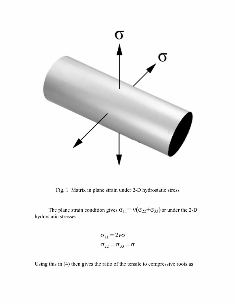
Fig. 1 Matrix in plane strain under 2-D hydrostatic stress The plane strain condition gives !11= #(!22+!33) or under the 2-D hydrostatic stresses

!11 = 2"!!22 = ! 33 = !

Using this in (4) then gives the ratio of the tensile to compressive roots as

! = ! +

! " =" 1+"( ) 1" #( )+ 1+"( )2 1" #( )2 + 1" 2"( )2 #1+"( ) 1" #( )+ 1+"( )2 1" #( )2 + 1" 2"( )2 #

where # is the matrix material Poisson’s ratio and

! = TC

for the isotropic matrix material. Next, in the composite material the matrix controlled failure criterion (1) will be taken to have the same ratio of transverse hydrostatic tensile and compressive failure stresses as that for the matrix material itself, since the matrix material controls the failure in this situation. The reason for using the equal biaxial stress state rather than a uniaxial stress state is that macroscopic 2-D pressure produces a much simpler micromechanics level stress state than does macro uniaxial stress in the transverse direction. The equal biaxial transverse stresses !22 = !33 in (1) gives the roots as

!22C22

= 1"

# 1# $22( ) ± 1# $22( )2 + $22"% & '

( ) *

where

!22 = T22C22

and

(7)

(8)

! = 4 " T22C22S232

# $ %

& ' (

The equal biaxial stress roots ratio can be formed from (8) as

!22+

!22"

As already mentioned, this composite material ratio from (8) will be set equal to the corresponding matrix material ratio from (7). This equality of these two ratios at the two different scales is not expected to be true in all fiber composite materials cases, but it will be use here in the special case, (6), which is taken to be the guiding case with which to calibrate general behavior and thereby evaluate " in (5). That is, the properties in (6) are the most typical and common values usually reported and they will be used here to find the value of ". Setting

!22+ /! 22

" from (8) equal to the like ratio (7) for the matrix

material gives an equation to be solved for S23, the property that is so difficult to determine experimentally. After lengthy reduction, but no approximations, it is found that this procedure gives

S232 = 1!"( )2

4 1! T22C22

"# $ %

& ' ( 1!

C22T22

"# $ %

& ' (

)

*

+ + + +

,

-

.

.

.

.

T22C22

where $ is given by the matrix properties in (7).

(9)

The micromechanics result (9) is close to the expected form (5) but it is not quite there yet. To bring (9) into alignment with (5) the nondimensional coefficient of T22 C22 in (9) will be evaluated for the calibrating special properties in (6). To carry out this process first use the matrix properties in (6) to determine $ in (7). This gives

! = 22 " 422 + 4

Using this value for $ and T22/C22 from (6) in (9) gives, after much consolidation of terms but no approximations

S232 = 2

7T22C22

This now has the expected form, that of (5). Relation (10) is the explicit macroscopic result for the S23 property obtained from the micromechanics derivation for carbon-epoxy composites. It has considerable utility in applications since it obviates the need to experimentally determine S23 with all its attendant problems. With relation (10) combined with failure criteria (1) and (2), there are now five independent failure properties for aligned fiber composites. This is the same as the number of independent elastic properties for transverse isotropy. A further interpretation of (10) will now be given. It is interesting to observe that the result (10) falls within some likely bounds for S23 for carbon fiber composite materials. Consider the general case of aligned fiber composite materials when the fiber stiffness is varied over the full range possible. At the lower limit where the fibers have the

(10)

same stiffness as the matrix material, then the value for S23 must be the same as that for an isotropic material, namely

S232 = T22C22

3

At the other limit, the foregoing failure forms (1) and (3) show that there must be

S232 > T22C22

4

If S23 varies monotonically between these two limits, as it likely does, then it is seen that the result (10) with the coefficient of 2/7 fits in right between the above two limits of 2/6 and 2/8. Finally, three examples will be given. These examples have the T22/C22 ratios of 1/4, 1/3, and 1/2.4. These cover the usual range found for this properties ratio. For Example 1 take

T22 = 50 MPaC22 = 200 MPa

Then (10) gives S23 as

S23 = 53.5 MPa In equal biaxial tension and compression the roots from (8) are

!22+ = 31.6 MPa

!22" = "632MPa

For Example 2 take

T22 = 50 MPaC22 =150 MPa

This example corresponds to that of the calibrating case in (6). From (10) there follows

S23 = 46.3MPa and from (8) the equal biaxial failure stresses are

!22+ = 34.6 MPa

!22" = "435MPa

The third example has

T22 = 50 MPaC22 =120 MPa

From (10) there is

S23 = 41.4 MPa and from (8)

!22+ = 37.8 MPa

!22" = "318MPa

It is seen that quite large stress levels are required to fail these materials in equal biaxial compressive stress states. Nevertheless these materials can and must fail in these transverse stress states, as can be reasoned independently. The final form (10) derived from micromechanics greatly facilitates the three dimensional application of failure criterion (1).

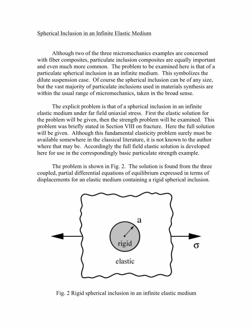
Spherical Inclusion in an Infinite Elastic Medium Although two of the three micromechanics examples are concerned with fiber composites, particulate inclusion composites are equally important and even much more common. The problem to be examined here is that of a particulate spherical inclusion in an infinite medium. This symbolizes the dilute suspension case. Of course the spherical inclusion can be of any size, but the vast majority of particulate inclusions used in materials synthesis are within the usual range of micromechanics, taken in the broad sense. The explicit problem is that of a spherical inclusion in an infinite elastic medium under far field uniaxial stress. First the elastic solution for the problem will be given, then the strength problem will be examined. This problem was briefly stated in Section VIII on fracture. Here the full solution will be given. Although this fundamental elasticity problem surely must be available somewhere in the classical literature, it is not known to the author where that may be. Accordingly the full field elastic solution is developed here for use in the correspondingly basic particulate strength example. The problem is shown in Fig. 2. The solution is found from the three coupled, partial differential equations of equilibrium expressed in terms of displacements for an elastic medium containing a rigid spherical inclusion.

Fig. 2 Rigid spherical inclusion in an infinite elastic medium

The solution is given in spherical coordinates with the polar axis % = 0 being in the uniaxial stress direction. The displacement solution is given by

E!ur = 1" 2#( )

3r " a

3

r2$ % &

' ( ) +

1+#3

$ %

' ( r "

5 5 " 4#( )4 4 " 5#( )

a3

r2+ 94 4 " 5#( )

a5

r4*

+ ,

-

. / 2cos

20 " sin20( )

E!u0 = 1+#( ) "r + 5 1" 2#( )

2 4 " 5#( )a3

r2+ 32 4 " 5#( )

a5

r4*

+ ,

-

. / sin0 cos0

Displacement component u& vanishes since the problem is axi-symmetric. Symbol ! is the applied far field uniaxial stress. The complete stress field is found to be given by

(11)

! rr!

= cos2" + 231# 2$1+$

% &

' ( ar

% &

' (

3

+

14 # 5$

# 565 #$( ) a

r% &

' (

3

+ 3 ar

% &

' (

5)

* +

,

- . sin2" +

14 # 5$

535 #$( ) a

r% &

' (

3

# 6 ar

% &

' (

5)

* +

,

- . cos2"

!""!

= sin2" # 131# 2$1+$

% &

' ( ar

% &

' (

3

#

14 # 5$

5121# 2$( ) a

r% &

' (

3

+ 94

ar

% &

' (

5)

* +

,

- . sin2" +

14 # 5$

# 531# 2$( ) a

r% &

' (

3

+ 3 ar

% &

' (

5)

* +

,

- . cos2"

!//

!= # 1

31# 2$1+$

% &

' ( ar

% &

' (

3

+

14 # 5$

2512

1# 2$( ) ar

% &

' (

3

# 34

ar

% &

' (

5)

* +

,

- . sin2" +

14 # 5$

# 531# 2$( ) a

r% &

' (

3

+ 3 ar

% &

' (

5)

* +

,

- . cos2"

! r"!

= #1+ 52

1+$4 # 5$

% &

' ( ar

% &

' (

3

# 64 # 5$( )

ar

% &

' (

5)

* +

,

- . sin" cos"

The other two shear stress components vanish.

(12)

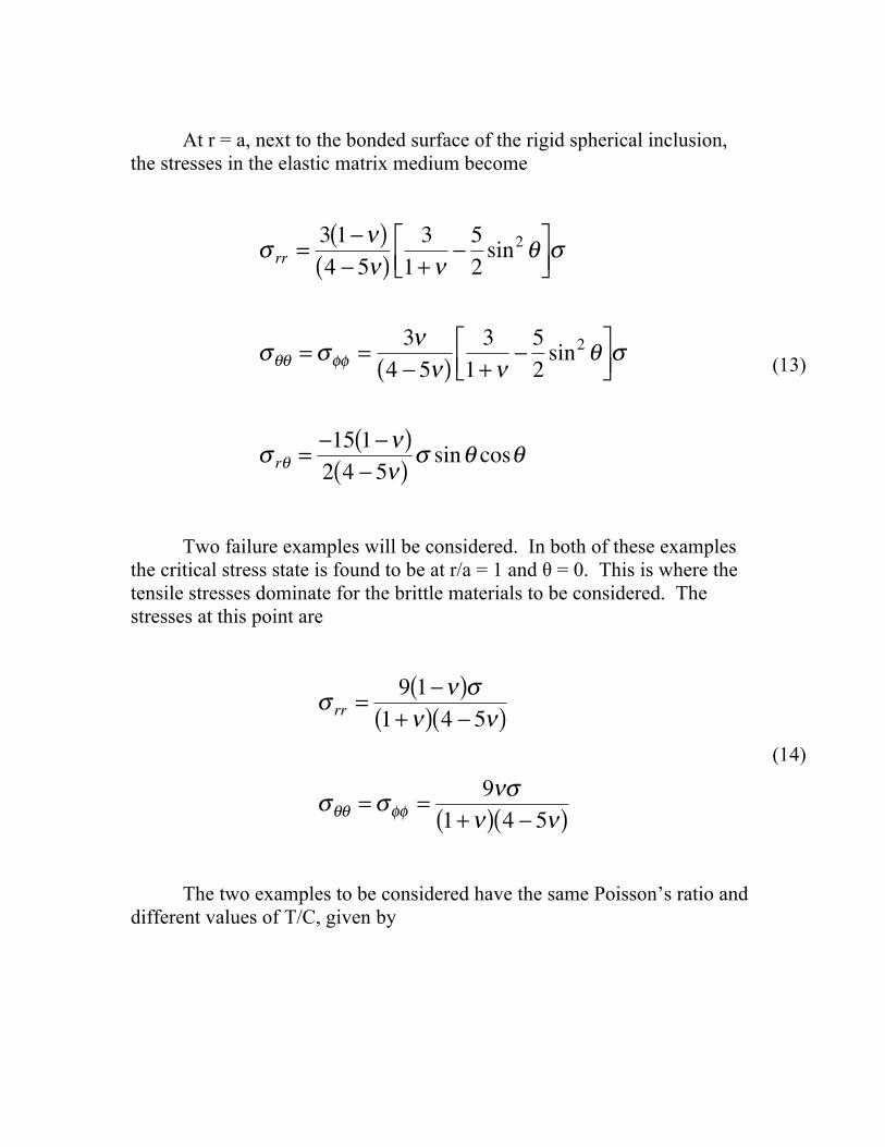
At r = a, next to the bonded surface of the rigid spherical inclusion, the stresses in the elastic matrix medium become

! rr = 3 1"#( )4 " 5#( )

31+#

" 52sin2$%

& ' ( ) * !

!$$ = !++ = 3#4 " 5#( )

31+#

" 52sin2$%

& ' ( ) * !

! r$ = "15 1"#( )2 4 " 5#( ) ! sin$ cos$

Two failure examples will be considered. In both of these examples the critical stress state is found to be at r/a = 1 and % = 0. This is where the tensile stresses dominate for the brittle materials to be considered. The stresses at this point are

! rr = 9 1"#( )!1+#( ) 4 " 5#( )

!$$ = !%% = 9#!1+#( ) 4 " 5#( )

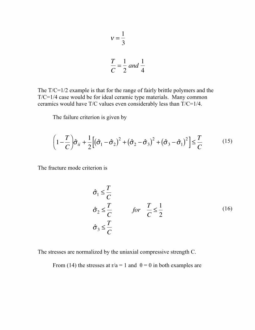
The two examples to be considered have the same Poisson’s ratio and different values of T/C, given by

(13)

(14)

! = 13

TC

= 12and 1

4

The T/C=1/2 example is that for the range of fairly brittle polymers and the T/C=1/4 case would be for ideal ceramic type materials. Many common ceramics would have T/C values even considerably less than T/C=1/4. The failure criterion is given by

1! TC

" #

$ %

ˆ & ii + 12

ˆ & 1 ! ˆ & 2( )2 + ˆ & 2 ! ˆ & 3( )2 + ˆ & 3 ! ˆ & 1( )2[ ] ' TC

The fracture mode criterion is

ˆ ! 1 "TC

ˆ ! 2 "TC

for TC" 1

2

ˆ ! 3 "TC

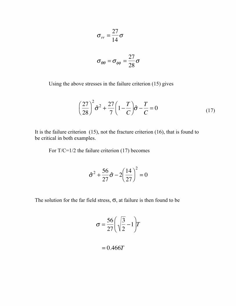
The stresses are normalized by the uniaxial compressive strength C. From (14) the stresses at r/a = 1 and % = 0 in both examples are

(15)

(16)

! rr = 2714

!

!"" = !## = 2728

!

Using the above stresses in the failure criterion (15) gives

2728

! "

# $

2ˆ % 2 + 27

71& T

C! "

# $

ˆ % & TC

= 0

It is the failure criterion (15), not the fracture criterion (16), that is found to be critical in both examples. For T/C=1/2 the failure criterion (17) becomes

ˆ ! 2 + 5627

ˆ ! " 2 1427

# $

% &

2

= 0

The solution for the far field stress, !, at failure is then found to be

! = 5627

32"1

# $ %

& ' ( T

= 0.466T

(17)

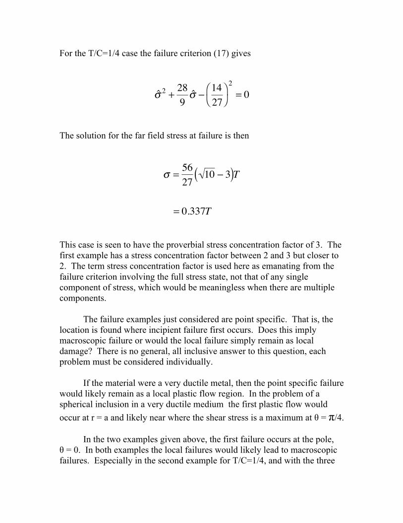
For the T/C=1/4 case the failure criterion (17) gives

ˆ ! 2 + 289

ˆ ! " 1427

# $

% &

2

= 0

The solution for the far field stress at failure is then

! = 5627

10 " 3( )T

= 0.337T

This case is seen to have the proverbial stress concentration factor of 3. The first example has a stress concentration factor between 2 and 3 but closer to 2. The term stress concentration factor is used here as emanating from the failure criterion involving the full stress state, not that of any single component of stress, which would be meaningless when there are multiple components. The failure examples just considered are point specific. That is, the location is found where incipient failure first occurs. Does this imply macroscopic failure or would the local failure simply remain as local damage? There is no general, all inclusive answer to this question, each problem must be considered individually. If the material were a very ductile metal, then the point specific failure would likely remain as a local plastic flow region. In the problem of a spherical inclusion in a very ductile medium the first plastic flow would occur at r = a and likely near where the shear stress is a maximum at % = '/4. In the two examples given above, the first failure occurs at the pole, % = 0. In both examples the local failures would likely lead to macroscopic failures. Especially in the second example for T/C=1/4, and with the three

dimensional, far field tensile stress state, it is very likely that the local failure would take the form of a brittle crack(s) that would easily and quickly propagate throughout the material. In treating problems of this type using isotropic macroscopic failure criteria, micromechanics analysis such as given here, are very helpful in understanding what nucleates the macroscopic failure. Load Redistribution in Aligned Fiber Composites The function of the matrix phase in aligned fiber composite materials is often misunderstood and usually completely undervalued. The matrix is seen as little more than a space filling medium between the fibers that can accommodate fittings and attachments. The real and vital function of the matrix phase is best understood through micromechanics. One example has already been given in the first subsection of this section. Another important function will now be examined. In the introduction to this section it was mentioned that the state of flaws and defects are usually the nucleating sites for failure in fiber composites. Chief among such defects are broken filaments in the fiber bundles, fiber slack and variability along the fiber filaments. The matrix phase supplies the palliative that largely overcomes these defects. Without the matrix phase it would be virtually impossible to utilize the extraordinary properties that are inherent in carbon fibers and other high performance fibers. The load rebalancing or redistribution function of the matrix phase in transferring load around broken fibers provides the perfect example to illuminate the true role of the matrix phase. As will be seen, the key to performance in composites lies in the interaction between the high performance fibers and the coordinating matrix phase. This is an interaction that must extract the most from the fibers but cannot do so without the perfect complement of matrix properties.

Boundary Layer Theory It is advantageous to start with a quick summary and example of the macroscopic boundary layer theory for highly anisotropic fiber composites because it will pinpoint the properties and features that are needed in the micromechanics model for load redistribution. This boundary layer theory for fiber composites was developed by Pipkin and by Spencer and others. The outline given here follows from that of Christensen [1]. The boundary layer theory starts by recognizing that at the lamina level carbon fiber composites are highly anisotropic. Accordingly a simplified method of analysis is sought for this class of materials. It begins by identifying a small nondimensional parameter that can be used in the analysis. This rather obvious small parameter is given by

!2 = µ12E11 / 1"#12#21( )

where the lamina is in a plane stress state with E11 being the fiber direction modulus, µ12 the axial shear modulus and the other terms are the Poisson’s ratios. All other moduli type properties are taken to be of the same order as µ12. One more step is needed. In order to give a clear view of the thin boundary layer, the transverse direction coordinate x2 is “stretched” to the coordinate ( by taking

x2 = !" The complete formulation can be arranged with terms expressed as powers of ). By retaining only the lowest order terms in ), a fortunate thing happens. The entire formulation is found to reduce to and be governed by the following differential equations for the displacements

(18)

(19)

! 2u1!x12 + ! 2u1

!"2= 0

! 2u2!"2

= 0

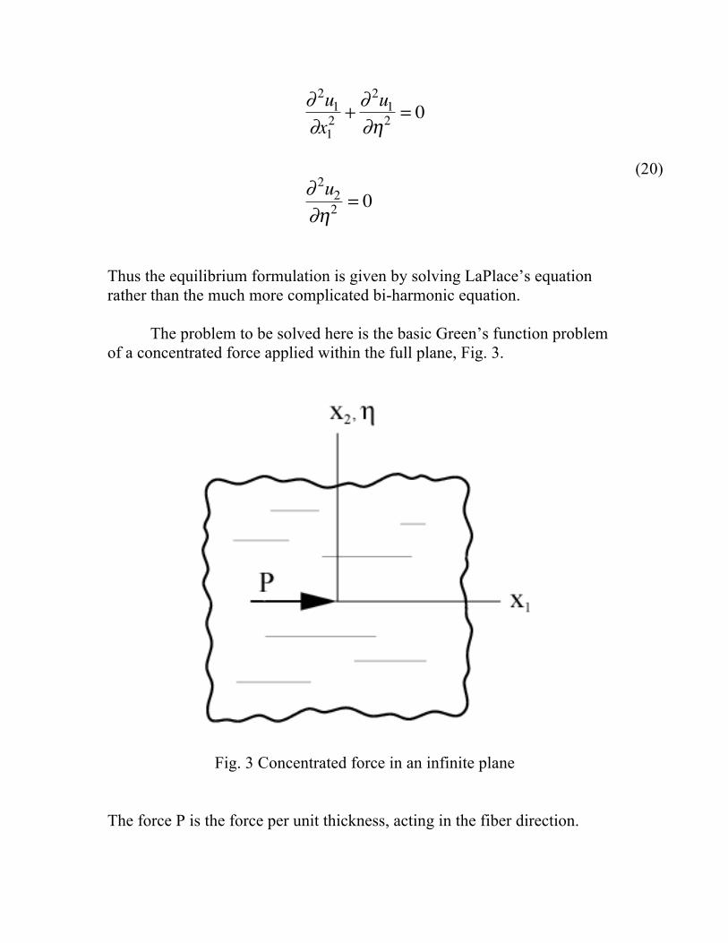
Thus the equilibrium formulation is given by solving LaPlace’s equation rather than the much more complicated bi-harmonic equation. The problem to be solved here is the basic Green’s function problem of a concentrated force applied within the full plane, Fig. 3.

Fig. 3 Concentrated force in an infinite plane The force P is the force per unit thickness, acting in the fiber direction.

(20)

The displacements are solved from (20) and the stresses, to consistent order in ), are then given by

!11 = " P2#$

x1x12 +%2( )

!12 = " P2#

%x12 +%2( )

!22 = 0

For high anisotropy, as occurs here, the Poisson’s ratios in (18) can be neglected and the stresses (21) at x2=0 and at x1=0 are given by

!11 x2=0 = " P2#

E11µ12

1x1

$ % &

' ( )

!12 x1=0 = " P2#

µ12E11

1x2

$ % &

' ( )

It is seen from these results that the characterizing stresses are !11 and !12. Both have singularities but !11 decays much more slowly with distance x1 from P than does !12 decay with respect to distance x2 from P. Stress !22 does not even enter the problem. All of this is the boundary layer effect. For infinitely stiff fibers the load is transmitted indefinitely along a singular line with no load being diffused out of it since the lateral shear stress vanishes.

(21)

(22)

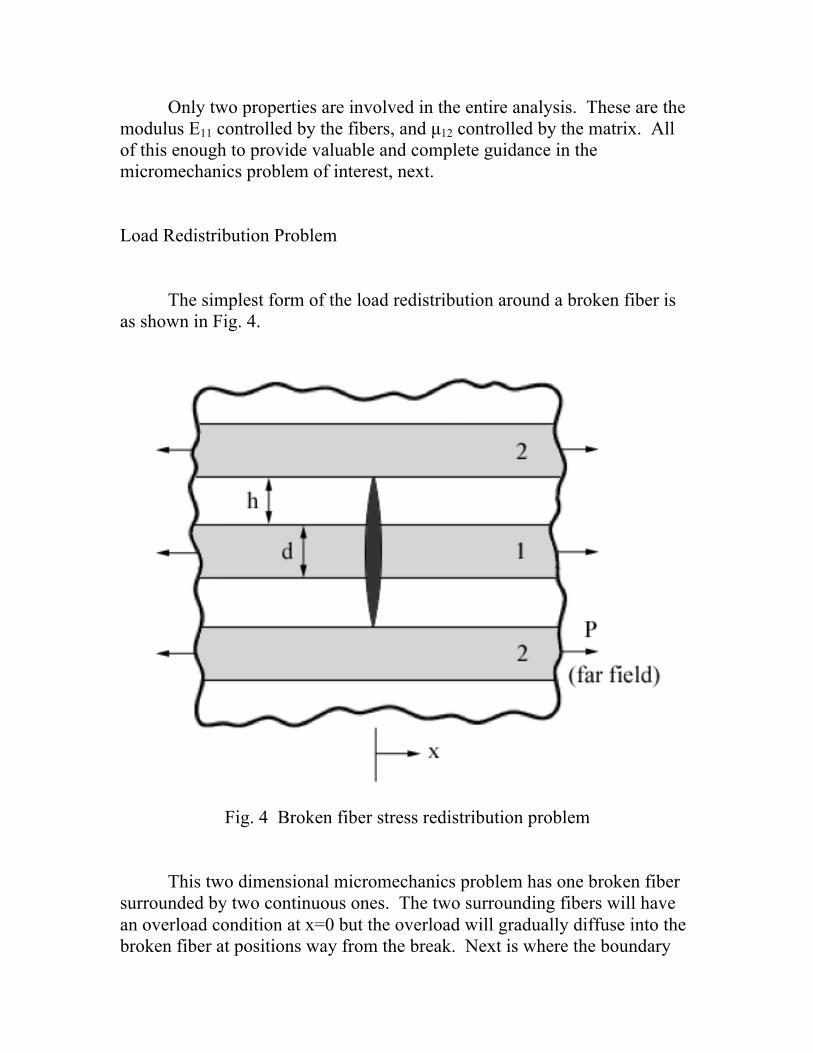
Only two properties are involved in the entire analysis. These are the modulus E11 controlled by the fibers, and µ12 controlled by the matrix. All of this enough to provide valuable and complete guidance in the micromechanics problem of interest, next. Load Redistribution Problem The simplest form of the load redistribution around a broken fiber is as shown in Fig. 4.

Fig. 4 Broken fiber stress redistribution problem This two dimensional micromechanics problem has one broken fiber surrounded by two continuous ones. The two surrounding fibers will have an overload condition at x=0 but the overload will gradually diffuse into the broken fiber at positions way from the break. Next is where the boundary

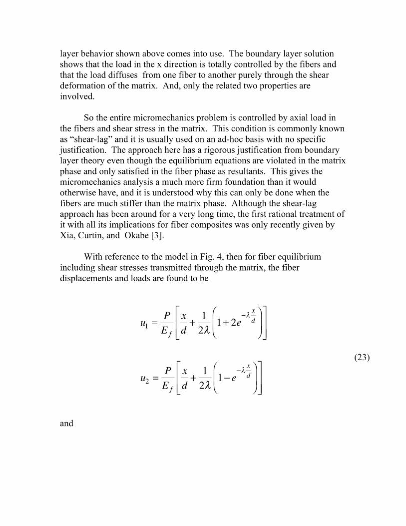
layer behavior shown above comes into use. The boundary layer solution shows that the load in the x direction is totally controlled by the fibers and that the load diffuses from one fiber to another purely through the shear deformation of the matrix. And, only the related two properties are involved. So the entire micromechanics problem is controlled by axial load in the fibers and shear stress in the matrix. This condition is commonly known as “shear-lag” and it is usually used on an ad-hoc basis with no specific justification. The approach here has a rigorous justification from boundary layer theory even though the equilibrium equations are violated in the matrix phase and only satisfied in the fiber phase as resultants. This gives the micromechanics analysis a much more firm foundation than it would otherwise have, and it is understood why this can only be done when the fibers are much stiffer than the matrix phase. Although the shear-lag approach has been around for a very long time, the first rational treatment of it with all its implications for fiber composites was only recently given by Xia, Curtin, and Okabe [3]. With reference to the model in Fig. 4, then for fiber equilibrium including shear stresses transmitted through the matrix, the fiber displacements and loads are found to be

u1 = PE f

xd

+ 12!

1+ 2e"! x

d#

$ % &

' ( )

* + +

,

- . .

u2 = PE f

xd

+ 12!

1" e"! x

d#

$ % &

' ( )

* + +

,

- . .

and

(23)

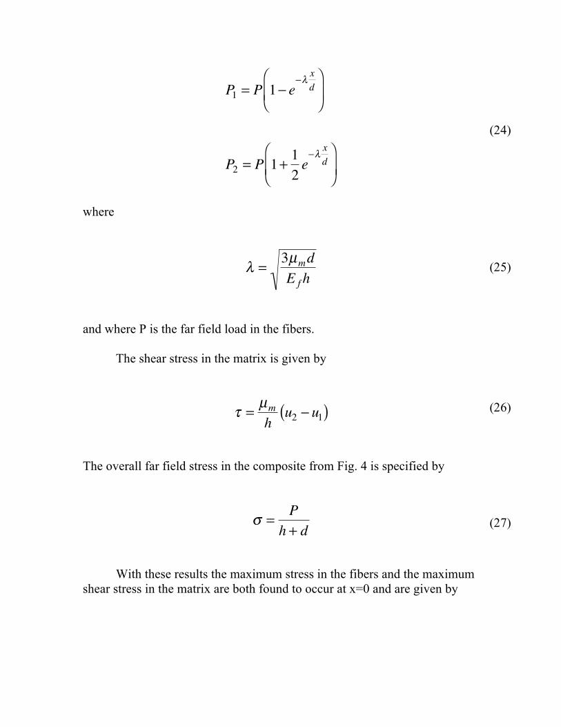
P1 = P 1! e!" x

d#

$ % &

' (

P2 = P 1+ 12e!" x

d#

$ % &

' (

where

! = 3µmdE f h

and where P is the far field load in the fibers. The shear stress in the matrix is given by

! = µmh

u2 " u1( )

The overall far field stress in the composite from Fig. 4 is specified by

! = Ph + d

With these results the maximum stress in the fibers and the maximum shear stress in the matrix are both found to occur at x=0 and are given by

(24)

(25)

(26)

(27)

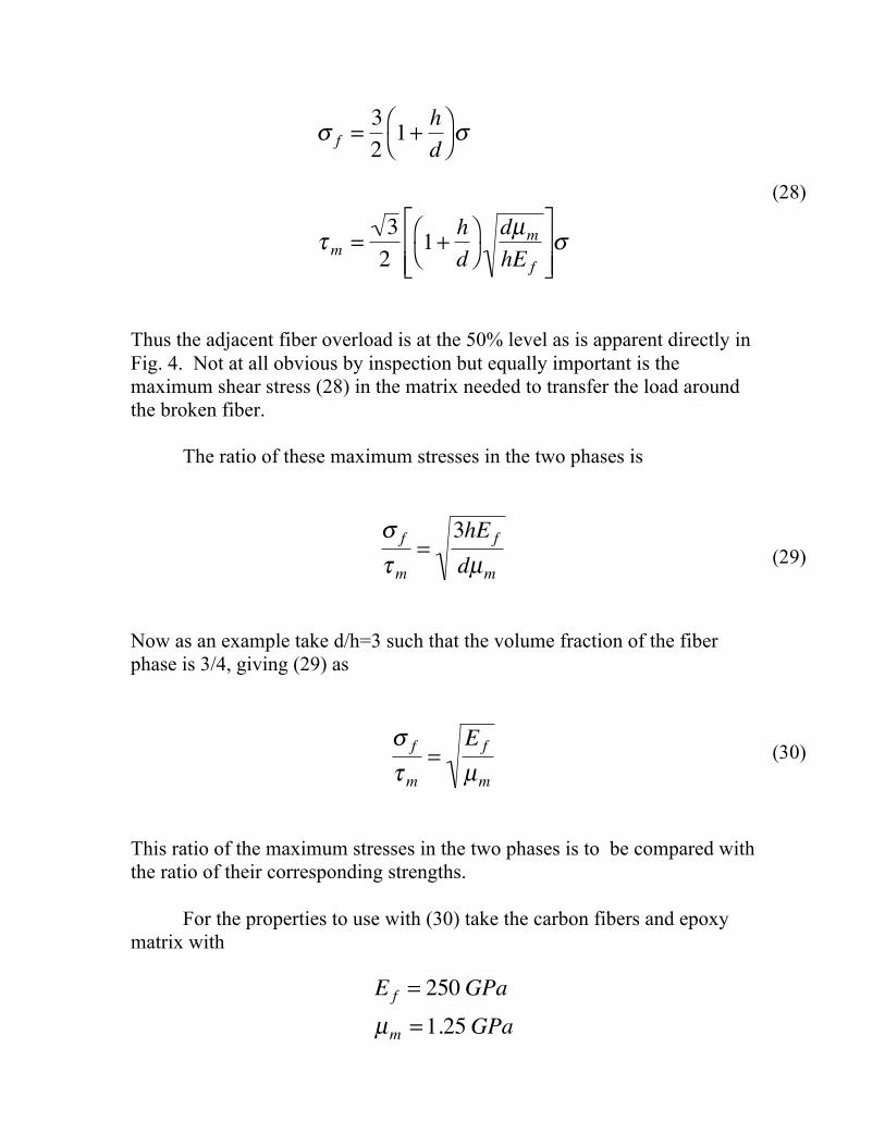
! f = 321+ h

d" #

$ % !

&m = 32

1+ hd

" #

$ %

dµmhE f

'

( ) )

*

+ , , !

Thus the adjacent fiber overload is at the 50% level as is apparent directly in Fig. 4. Not at all obvious by inspection but equally important is the maximum shear stress (28) in the matrix needed to transfer the load around the broken fiber. The ratio of these maximum stresses in the two phases is

! f

"m=

3hE f

dµm

Now as an example take d/h=3 such that the volume fraction of the fiber phase is 3/4, giving (29) as

! f

"m=

E f

µm

This ratio of the maximum stresses in the two phases is to be compared with the ratio of their corresponding strengths. For the properties to use with (30) take the carbon fibers and epoxy matrix with

E f = 250GPaµm =1.25GPa

(28)

(29)

(30)

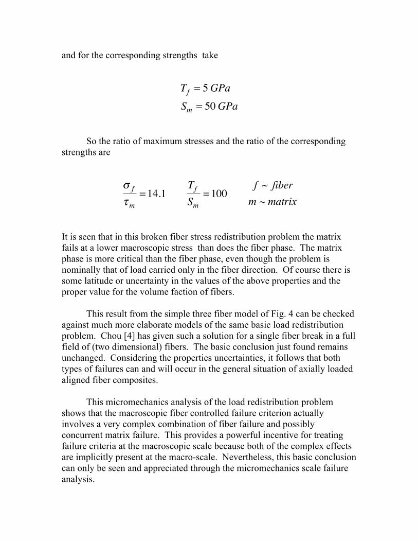
and for the corresponding strengths take

Tf = 5GPaSm = 50GPa

So the ratio of maximum stresses and the ratio of the corresponding strengths are

! f

"m=14.1

TfSm

=100f ~ fiberm ~ matrix

It is seen that in this broken fiber stress redistribution problem the matrix fails at a lower macroscopic stress than does the fiber phase. The matrix phase is more critical than the fiber phase, even though the problem is nominally that of load carried only in the fiber direction. Of course there is some latitude or uncertainty in the values of the above properties and the proper value for the volume faction of fibers. This result from the simple three fiber model of Fig. 4 can be checked against much more elaborate models of the same basic load redistribution problem. Chou [4] has given such a solution for a single fiber break in a full field of (two dimensional) fibers. The basic conclusion just found remains unchanged. Considering the properties uncertainties, it follows that both types of failures can and will occur in the general situation of axially loaded aligned fiber composites. This micromechanics analysis of the load redistribution problem shows that the macroscopic fiber controlled failure criterion actually involves a very complex combination of fiber failure and possibly concurrent matrix failure. This provides a powerful incentive for treating failure criteria at the macroscopic scale because both of the complex effects are implicitly present at the macro-scale. Nevertheless, this basic conclusion can only be seen and appreciated through the micromechanics scale failure analysis.

Although it is very difficult to quantitatively predict macroscopic failure from micro-scale, nano-scale or atomic scale considerations, these sub-scale analyses are still vital and indeed irreplacable. All new materials and most major advancements in existing materials start as concepts at the atomic, nano, or micro-scale levels. It is extremely important to understand the physical behavior at all scales even though the applications are dominantly macro-scale. References

1. Christensen, R. M., 2005, Mechanics of Composite Materials, Dover, New York.

2. Ha, S. K., Huang, Y., Han, H. H., and Jin, K. K., 2010,

“Micromechanics of Failure for Ultimate Strength Predictions of Composite Laminates”, J. Composite Materials, 44, 2347-2361.

3. Xia, Z., Curtin, W. A., and Okabe, T., 2002, “Green’s Function vs.

Shear-Lag Models of Damage and Failure in Fiber Composites”, Composites Science and Technology, 62, 1279-1288.

4. Chou, T. W., 1992, Microstructural Design of Fiber Composites,

Cambridge Univ. Press, Cambridge U.K.

Richard M. Christensen February 1st, 2011

Copyright © 2011 Richard M. Christensen