Embed Size (px)
Citation preview
ITERATIVE PROJECTION METHODS FORSPARSE LINEAR SYSTEMS AND
EIGENPROBLEMSCHAPTER 12 : AMLS METHOD
Heinrich [email protected]
Hamburg University of TechnologyInstitute of Numerical Simulation
TUHH Heinrich Voss AMLS Summer School 2006 1 / 45
Automated Multi-Level Substructuring
AMLS was introduced by Bennighof (1998) and was applied to huge problemsof frequency response analysis.
The large finite element model is recursively divided into very manysubstructures on several levels based on the sparsity structure of the systemmatrices.
Assuming that the interior degrees of freedom of substructures dependquasistatically on the interface degrees of freedom, and modeling thedeviation from quasistatic dependence in terms of a small number of selectedsubstructure eigenmodes the size of the finite element model is reducedsubstantially yet yielding satisfactory accuracy over a wide frequency range ofinterest.
Recent studies in vibro-acoustic analysis of passenger car bodies where verylarge FE models with more than six million degrees of freedom appear andseveral hundreds of eigenfrequencies and eigenmodes are needed haveshown that AMLS is considerably faster than Lanczos type approaches.
TUHH Heinrich Voss AMLS Summer School 2006 2 / 45

Condensation
Given (a finite element model of a structure, e.g.)
Kx = λMx (1)
where K ∈ Rn×n and M ∈ Rn×n are symmetric and M is positive definite.
Aim: Reduce the number of unknowns by some sort of elimination.
TUHH Heinrich Voss AMLS Summer School 2006 3 / 45
Exact condensation
Partition degrees of freedom into variables xi to be kept (for substructurings:interface DoF) and variables x` to be droped (local DoF). After reorderingproblem (1) obtains the following form
(K`` K`iKi` Kii
) (x`
xi
)= λ
(M`` M`iMi` Mii
) (x`
xi
)(2)
Solving the first equation for x` yields
x` = −(K`` − λM``)−1(K`i − λM`i)xi
and substituting in the second equation one gets the exactly condensedeigenproblem
T (λ)xi = −Kiixi + λMiixi + (Ki` − λMi`)(K`` − λM``)−1(K`i − λM`i)xi
TUHH Heinrich Voss AMLS Summer School 2006 4 / 45
Static condensation
Linearizing the exactly condensed problem at ω = 0 yields the staticallycondensed eigenproblem (introduced independently by Irons (1965) andGuyan (1965))
Kiixi = λMiixi (3)
where
Kii = Kii − Ki`K−1`` K`i
Mii = Mii − Ki`K−1`` M`i − M`iK−1
`` K`i + Ki`K−1`` M``K−1
`` K`i
For vibrating structures this means that the local degrees of freedom areassumed to depend quasistatically on the interface degrees of freedom, andthe inertia forces of the substructures are neglected.
TUHH Heinrich Voss AMLS Summer School 2006 5 / 45
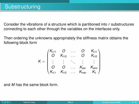
Substructuring
Consider the vibrations of a structure which is partitioned into r substructuresconnecting to each other through the variables on the interfaces only.
Then ordering the unknowns appropriately the stiffness matrix obtains thefollowing block form
K =
K``1 O . . . O K`i1O K``2 . . . O K`i2...
.... . .
......
O O . . . Kssr KsmrKi`1 Ki`2 . . . Kmsr Kii
and M has the same block form.
TUHH Heinrich Voss AMLS Summer School 2006 6 / 45
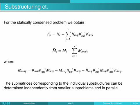
Substructuring ct.
For the statically condensed problem we obtain
Kii = Kii −r∑
j=1
KmsjK−1ssj Ksmj
Mii = Mii −r∑
j=1
Mmmj ,
where
Mmmj = KmsjK−1ssj Msmj + MmsjK−1
ssj Ksmj − KmsjK−1ssj MssjK−1
ssj Ksmj .
The submatrices corresponding to the individual substructures can bedetermined independently from smaller subproblems and in parallel.
TUHH Heinrich Voss AMLS Summer School 2006 7 / 45
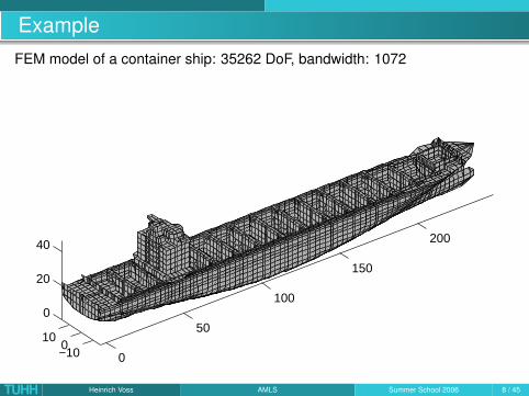
ExampleFEM model of a container ship: 35262 DoF, bandwidth: 1072
0
50
100
150
200
−100
10
0
20
40
TUHH Heinrich Voss AMLS Summer School 2006 8 / 45
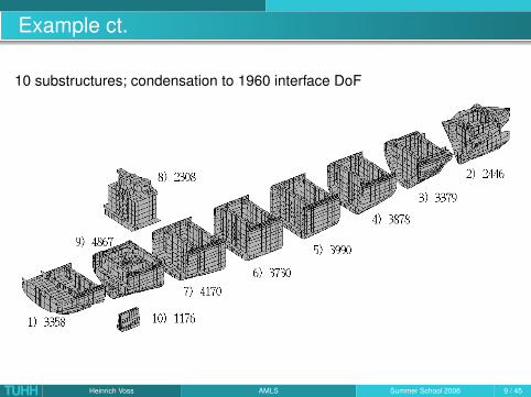
Example ct.
10 substructures; condensation to 1960 interface DoF
TUHH Heinrich Voss AMLS Summer School 2006 9 / 45
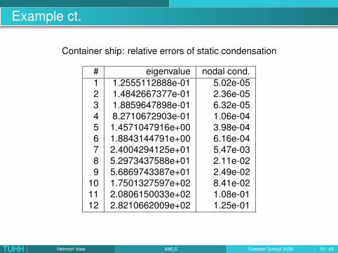
Example ct.
Container ship: relative errors of static condensation
# eigenvalue nodal cond.1 1.2555112888e-01 5.02e-052 1.4842667377e-01 2.36e-053 1.8859647898e-01 6.32e-054 8.2710672903e-01 1.06e-045 1.4571047916e+00 3.98e-046 1.8843144791e+00 6.16e-047 2.4004294125e+01 5.47e-038 5.2973437588e+01 2.11e-029 5.6869743387e+01 2.49e-02
10 1.7501327597e+02 8.41e-0211 2.0806150033e+02 1.08e-0112 2.8210662009e+02 1.25e-01
TUHH Heinrich Voss AMLS Summer School 2006 10 / 45

A projection approach
We transform the matrix K to block diagonal form using block Gaussianelimination, i.e. we apply the congruence transformation with
P =
(I −K−1
`` K`i0 I
)to the pencil (K , M) obtaining the equivalent pencil
(PT KP, PT MP) =
((K`` 00 Kii
),
(M`` M`i
Mi` Mii
)). (4)
Here K`` and M`` stay unchanged, and
Kii = Kii − Ki`K−1`` K`i is the Schur complement of K``
M`i = M`i − M``K−1`` K`i = MT
i`
Mii = Mii − Mi`K−1`` K`i − Ki`K−1
`` M`i + Ki`K−1`` M``K−1
`` K`i .
TUHH Heinrich Voss AMLS Summer School 2006 11 / 45
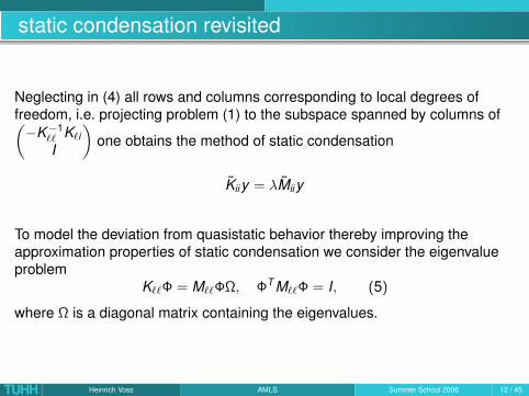
static condensation revisited
Neglecting in (4) all rows and columns corresponding to local degrees offreedom, i.e. projecting problem (1) to the subspace spanned by columns of(−K−1
`` K`iI
)one obtains the method of static condensation
Kiiy = λMiiy
To model the deviation from quasistatic behavior thereby improving theapproximation properties of static condensation we consider the eigenvalueproblem
K``Φ = M``ΦΩ, ΦT M``Φ = I, (5)
where Ω is a diagonal matrix containing the eigenvalues.
TUHH Heinrich Voss AMLS Summer School 2006 12 / 45
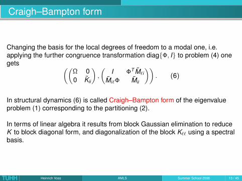
Craigh–Bampton form
Changing the basis for the local degrees of freedom to a modal one, i.e.applying the further congruence transformation diagΦ, I to problem (4) onegets ((
Ω 00 Kii
),
(I ΦT M`i
Mi`Φ Mii
)). (6)
In structural dynamics (6) is called Craigh–Bampton form of the eigenvalueproblem (1) corresponding to the partitioning (2).
In terms of linear algebra it results from block Gaussian elimination to reduceK to block diagonal form, and diagonalization of the block K`` using a spectralbasis.
TUHH Heinrich Voss AMLS Summer School 2006 13 / 45
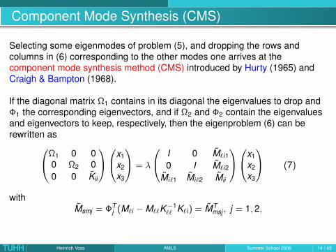
Component Mode Synthesis (CMS)
Selecting some eigenmodes of problem (5), and dropping the rows andcolumns in (6) corresponding to the other modes one arrives at thecomponent mode synthesis method (CMS) introduced by Hurty (1965) andCraigh & Bampton (1968).
If the diagonal matrix Ω1 contains in its diagonal the eigenvalues to drop andΦ1 the corresponding eigenvectors, and if Ω2 and Φ2 contain the eigenvaluesand eigenvectors to keep, respectively, then the eigenproblem (6) can berewritten asΩ1 0 0
0 Ω2 00 0 Kii
x1x2x3
= λ
I 0 M`i1
0 I M`i2
Mi`1 Mi`2 Mii
x1x2x3
(7)
withMsmj = ΦT
j (M`i − M``K−1`` K`i) = MT
msj , j = 1, 2,
TUHH Heinrich Voss AMLS Summer School 2006 14 / 45
CMS ct.
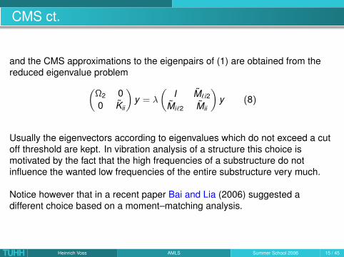
and the CMS approximations to the eigenpairs of (1) are obtained from thereduced eigenvalue problem(
Ω2 00 Kii
)y = λ
(I M`i2
Mi`2 Mii
)y (8)
Usually the eigenvectors according to eigenvalues which do not exceed a cutoff threshold are kept. In vibration analysis of a structure this choice ismotivated by the fact that the high frequencies of a substructure do notinfluence the wanted low frequencies of the entire substructure very much.
Notice however that in a recent paper Bai and Lia (2006) suggested adifferent choice based on a moment–matching analysis.
TUHH Heinrich Voss AMLS Summer School 2006 15 / 45
Container ship
We consider the structural deformation caused by a harmonic excitation at afrequency of 4 Hz which is a typical forcing frequency stemming from theengine and the propeller.
Since the deformation is small the assumptions of the linear theory apply, andthe structural response can be determined by the mode superposition methodtaking into account eigenfrequencies in the range between 0 and 7.5 Hz(which corresponds to the 50 smallest eigenvalues for the ship underconsideration).
To apply the CMS method we partitioned the FEM model into 10 substructuresas shown before. This substructuring by hand yielded a much smaller numberof interface degrees of freedom than automatic graph partitioners which try toconstruct a partition where the substructures have nearly equal size.
For instance, our model ends up with 1960 degrees of freedom on theinterfaces, whereas Chaco ends up with a substructuring into 10substructures with 4985 interface degrees of freedom.
TUHH Heinrich Voss AMLS Summer School 2006 16 / 45

Container ship ct.We solved the eigenproblem by the CMS method using a cut-off bound of20,000 (about 10 times the largest wanted eigenvalue λ50 ≈ 2183). 329eigenvalues of the substructure problems were less than our threshold, andthe dimension of the resulting projected problem was 2289.
0 10 20 30 40 5010
−8
10−7
10−6
10−5
10−4
10−3
10−2
CMS: cut off frequency 20000
number of eigenvalue
rela
tive
erro
r
TUHH Heinrich Voss AMLS Summer School 2006 17 / 45
Reducing interface DoF
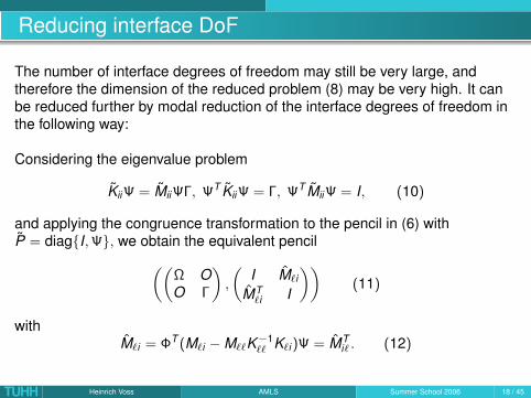
The number of interface degrees of freedom may still be very large, andtherefore the dimension of the reduced problem (8) may be very high. It canbe reduced further by modal reduction of the interface degrees of freedom inthe following way:
Considering the eigenvalue problem
KiiΨ = MiiΨΓ, ΨT KiiΨ = Γ, ΨT MiiΨ = I, (10)
and applying the congruence transformation to the pencil in (6) withP = diagI,Ψ, we obtain the equivalent pencil((
Ω OO Γ
),
(I M`i
MT`i I
))(11)
withM`i = ΦT (M`i − M``K−1
`` K`i)Ψ = MTi` . (12)
TUHH Heinrich Voss AMLS Summer School 2006 18 / 45
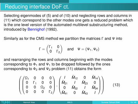
Reducing interface DoF ct.Selecting eigenmodes of (5) and of (10) and neglecting rows and columns in(11) which correspond to the other modes one gets a reduced problem whichis the one level version of the automated multilevel substructuring method,introduced by Bennighof (1992).
Similarly as for the CMS method we partition the matrices Γ and Ψ into
Γ =
(Γ1 00 Γ2
)and Ψ = (Ψ1,Ψ2)
and rearranging the rows and columns beginning with the modescorresponding to Φ1 and Ψ1 to be dropped followed by the onescorresponding to Φ2 and Ψ2 problem (11) obtains the form
Ω1 0 0 00 Γ1 0 00 0 Ω2 00 0 0 Γ2
,
I M12 0 M14
M21 I M23 00 M32 I M34
M41 0 M43 I
(13)
TUHH Heinrich Voss AMLS Summer School 2006 19 / 45
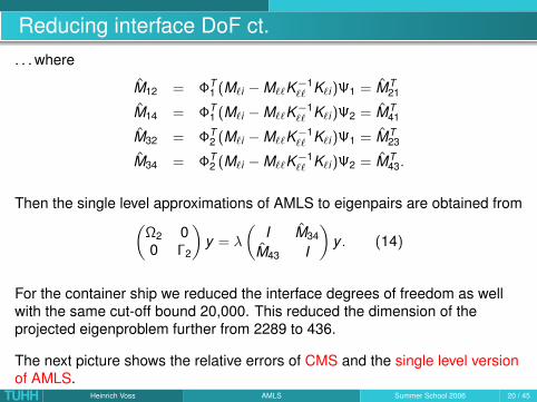
Reducing interface DoF ct.. . . where
M12 = ΦT1 (M`i − M``K−1
`` K`i)Ψ1 = MT21
M14 = ΦT1 (M`i − M``K−1
`` K`i)Ψ2 = MT41
M32 = ΦT2 (M`i − M``K−1
`` K`i)Ψ1 = MT23
M34 = ΦT2 (M`i − M``K−1
`` K`i)Ψ2 = MT43.
Then the single level approximations of AMLS to eigenpairs are obtained from(Ω2 00 Γ2
)y = λ
(I M34
M43 I
)y . (14)
For the container ship we reduced the interface degrees of freedom as wellwith the same cut-off bound 20,000. This reduced the dimension of theprojected eigenproblem further from 2289 to 436.
The next picture shows the relative errors of CMS and the single level versionof AMLS.
TUHH Heinrich Voss AMLS Summer School 2006 20 / 45
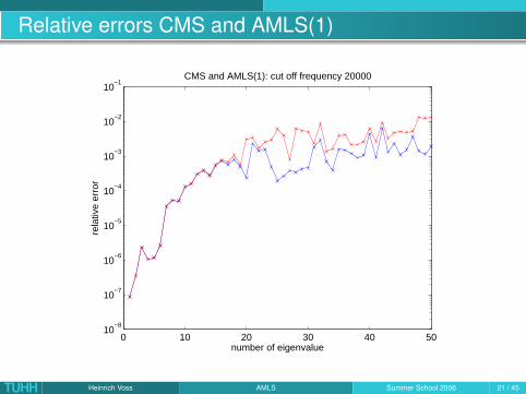
Relative errors CMS and AMLS(1)
0 10 20 30 40 5010
−8
10−7
10−6
10−5
10−4
10−3
10−2
10−1
number of eigenvalue
rela
tive
erro
r
CMS and AMLS(1): cut off frequency 20000
TUHH Heinrich Voss AMLS Summer School 2006 21 / 45

Multi-Level Substructuring: Level 0
TUHH Heinrich Voss AMLS Summer School 2006 22 / 45

Multi-Level Substructuring: Level 1
TUHH Heinrich Voss AMLS Summer School 2006 23 / 45
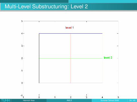
Multi-Level Substructuring: Level 2
TUHH Heinrich Voss AMLS Summer School 2006 24 / 45
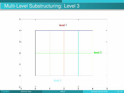
Multi-Level Substructuring: Level 3
TUHH Heinrich Voss AMLS Summer School 2006 25 / 45
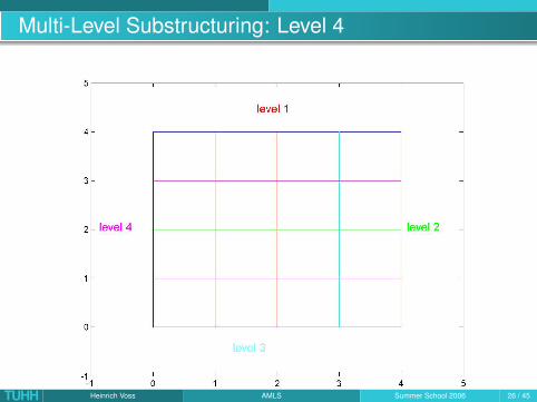
Multi-Level Substructuring: Level 4
TUHH Heinrich Voss AMLS Summer School 2006 26 / 45
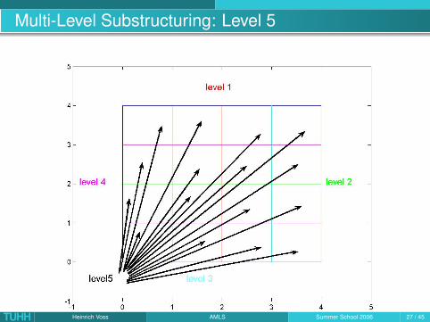
Multi-Level Substructuring: Level 5
TUHH Heinrich Voss AMLS Summer School 2006 27 / 45
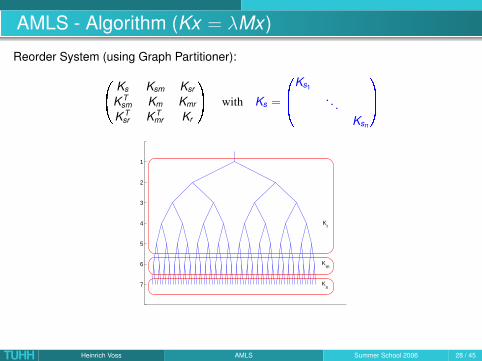
AMLS - Algorithm (Kx = λMx)
Reorder System (using Graph Partitioner):
0@
Ks Ksm Ksr
K Tsm Km Kmr
K Tsr K T
mr Kr
1A with Ks =
0B@
Ks1
. . .Ksn
1CA
7
6
5
4
3
2
1
Km
Ks
Kr
TUHH Heinrich Voss AMLS Summer School 2006 28 / 45
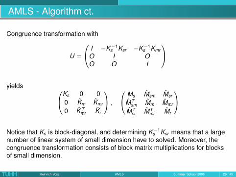
AMLS - Algorithm ct.
Congruence transformation with
U =
I −K−1s Ksr −K−1
s KmrO I OO O I
yields Ks 0 00 Km Kmr
0 K Tmr Kr
,
Ms Msm Msr
MTsm Mm Mmr
MTsr MT
mr Mr
Notice that Ks is block-diagonal, and determining K−1s Ksr means that a large
number of linear system of small dimension have to solved. Moreover, thecongruence transformation consists of block matrix multiplications for blocksof small dimension.
TUHH Heinrich Voss AMLS Summer School 2006 29 / 45
AMLS - Algorithm ct.
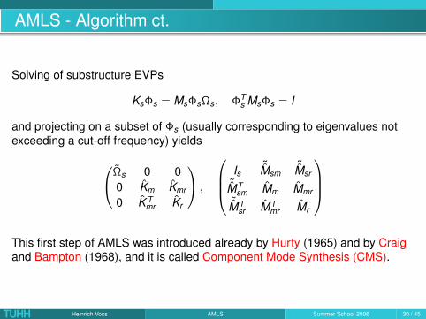
Solving of substructure EVPs
KsΦs = MsΦsΩs, ΦTs MsΦs = I
and projecting on a subset of Φs (usually corresponding to eigenvalues notexceeding a cut-off frequency) yields
Ωs 0 00 Km Kmr
0 K Tmr Kr
,
Is˜Msm
˜Msr˜MT
sm Mm Mmr˜MT
sr MTmr Mr
This first step of AMLS was introduced already by Hurty (1965) and by Craigand Bampton (1968), and it is called Component Mode Synthesis (CMS).
TUHH Heinrich Voss AMLS Summer School 2006 30 / 45
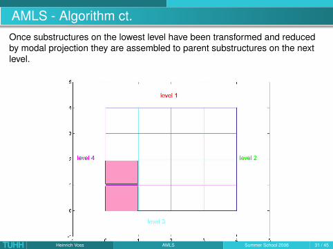
AMLS - Algorithm ct.Once substructures on the lowest level have been transformed and reducedby modal projection they are assembled to parent substructures on the nextlevel.
TUHH Heinrich Voss AMLS Summer School 2006 31 / 45
AMLS - Algorithm ct.
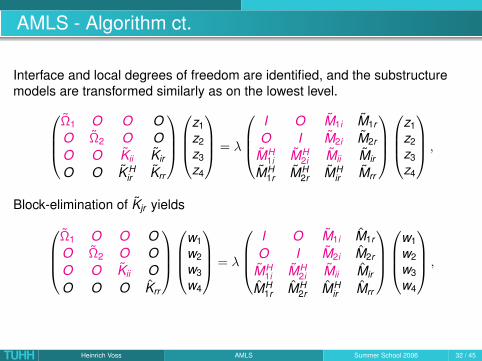
Interface and local degrees of freedom are identified, and the substructuremodels are transformed similarly as on the lowest level.
Ω1 O O OO Ω2 O OO O Kii Kir
O O K Hir Krr
z1z2z3z4
= λ
I O M1i M1r
O I M2i M2r
MH1i MH
2i Mii Mir
MH1r MH
2r MHir Mrr
z1z2z3z4
,
Block-elimination of Kjr yieldsΩ1 O O OO Ω2 O OO O Kii OO O O Krr
w1w2w3w4
= λ
I O M1i M1r
O I M2i M2r
MH1i MH
2i Mii Mir
MH1r MH
2r MHir Mrr
w1w2w3w4
,
TUHH Heinrich Voss AMLS Summer School 2006 32 / 45
AMLS - Algorithm ct.
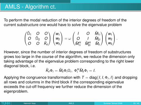
To perform the modal reduction of the interior degrees of freedom of thecurrent substructure one would have to solve the eigenvalue problemΩ1 O O
O Ω2 OO O Kii
w1w2w3
= ω
I O M1i
O I M2i
MH1i MH
2i Mii
w1w2w3
.
However, since the number of interior degrees of freedom of substructuresgrows too large in the course of the algorithm, we reduce the dimension onlytaking advantage of the eigenvalue problem corresponding to the right lowerdiagonal block, i.e.
KiiΦi = MiiΦiΩi , ΦHi MiiΦi = I.
Applying the congruence transformation with T = diagI, I,Φi , I and droppingall rows and columns in the third block if the corresponding eigenvalueexceeds the cut-off frequency we further reduce the dimension of theeigenproblem.
TUHH Heinrich Voss AMLS Summer School 2006 33 / 45
AMLS - Algorithm ct.
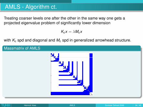
Treating coarser levels one after the other in the same way one gets aprojected eigenvalue problem of significantly lower dimension
Kcx = λMcx
with Kc spd and diagonal and Mc spd in generalized arrowhead structure.
Massmatrix of AMLS
TUHH Heinrich Voss AMLS Summer School 2006 34 / 45

Container shipWe substructured the FE model of the container ship by Metis with 4 levels ofsubstructuring. Neglecting eigenvalues exceeding 20,000 and 40,000 on alllevels AMLS produced a projected eigenvalue problem of dimension 451 and911, respectively.
0 5 10 15 20 25 30 35 40 45 5010
−7
10−6
10−5
10−4
10−3
10−2
10−1
100
TUHH Heinrich Voss AMLS Summer School 2006 35 / 45
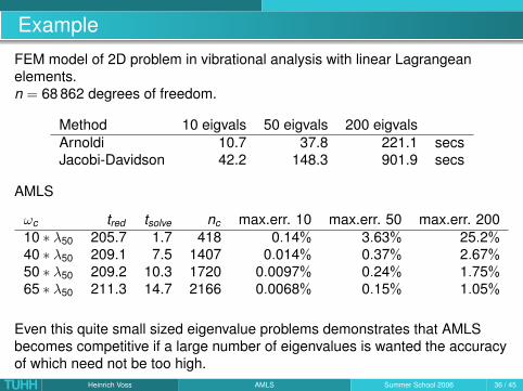
Example
FEM model of 2D problem in vibrational analysis with linear Lagrangeanelements.n = 68 862 degrees of freedom.
Method 10 eigvals 50 eigvals 200 eigvalsArnoldi 10.7 37.8 221.1 secsJacobi-Davidson 42.2 148.3 901.9 secs
AMLS
ωc tred tsolve nc max.err. 10 max.err. 50 max.err. 20010 ∗ λ50 205.7 1.7 418 0.14% 3.63% 25.2%40 ∗ λ50 209.1 7.5 1407 0.014% 0.37% 2.67%50 ∗ λ50 209.2 10.3 1720 0.0097% 0.24% 1.75%65 ∗ λ50 211.3 14.7 2166 0.0068% 0.15% 1.05%
Even this quite small sized eigenvalue problems demonstrates that AMLSbecomes competitive if a large number of eigenvalues is wanted the accuracyof which need not be too high.
TUHH Heinrich Voss AMLS Summer School 2006 36 / 45
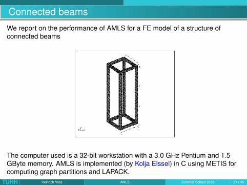
Connected beams
We report on the performance of AMLS for a FE model of a structure ofconnected beams
The computer used is a 32-bit workstation with a 3.0 GHz Pentium and 1.5GByte memory. AMLS is implemented (by Kolja Elssel) in C using METIS forcomputing graph partitions and LAPACK.
TUHH Heinrich Voss AMLS Summer School 2006 37 / 45
Connected beams ct.
For the following analysis a discretization with linear Lagrangean elementswith n = 517161 DoFs is used.
The AMLS method is applied with cut-off frequency ωc = 4 · 109.
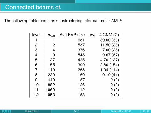
Due to the linear elements the matrices are relatively sparse resulting in smallinterfaces over all levels. Consequently, the eigenvalue problems are small aswell, which can be seen in the average size of the eigenvalue problems oneach level.
The distribution of component normal modes over the levels is typical for largescale problems. The average number of component normal modes (CNM) forthe interface and substructure eigenvalues problems that are below the cut-offfrequency decreases on lower levels. Quite commonly no CNMs are used forthe lowest level substructures.
TUHH Heinrich Voss AMLS Summer School 2006 38 / 45
Connected beams ct.
The following table contains substructuring information for AMLS
level nsub Avg.EVP size Avg. # CNM (Σ)1 1 681 39.00 (39)2 2 537 11.50 (23)3 4 376 7.00 (28)4 9 548 9.67 (87)5 27 425 4.70 (127)6 55 309 2.80 (154)7 110 268 1.04 (114)8 220 160 0.19 (41)9 440 87 0 (0)10 882 126 0 (0)11 1060 112 0 (0)12 953 153 0 (0)
TUHH Heinrich Voss AMLS Summer School 2006 39 / 45
Connected beams ct.
The limiting factors for the applicability of the algorithm are the computationaltime and the memory requirements. For the computations discussed externalstorage was used to store contemporary data and data needed forsubsequent calculations such as the computation of Ritz vectors. Thefollowing figure shows the memory consumption and the temporary storageneeded by the algorithm.
The large peak at the beginning of the calculation and in the middle are duethe graph partitioner which computes partitions for the graph corresponding tothe system matrices. For larger systems this becomes a limiting factor.
For systems which have a denser structure the size of the interface problemsbecome larger and cause problems with memory consumption and thesolution of the interface eigenvalue problems.
TUHH Heinrich Voss AMLS Summer School 2006 40 / 45
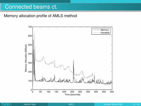
Connected beams ct.Memory allocation profile of AMLS method
0 50 100 150 200 250 300 350 400 450 5000
100
200
300
400
500
600
700
Time [seconds]
Mem
ory
Allo
catio
n [M
Byt
e]
MemoryHarddisk
TUHH Heinrich Voss AMLS Summer School 2006 41 / 45
Connected beams ct.
The computational time for this problem can be roughly divided into threeparts. With 60% the largest part of the computational time is spent on matrixmultiplications resulting from the variable transformations in step 2 of theAMLS algorithm.
The second largest part is with 20% due to the eigenvalue solver, followed bythe solution of linear systems of equations with 15%.
The remaining five percent consist of matrix partitioning (about 3%), matrixsubstructuring and algorithmic overhead.
Note, the matrix multiplications originating from the eigensolver and the linearsystem solver are included into their respective percentages and are notincluded in the percentage of the matrix multiplications.
TUHH Heinrich Voss AMLS Summer School 2006 42 / 45
Connected beams ct.
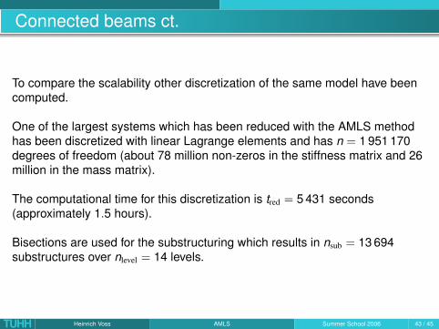
To compare the scalability other discretization of the same model have beencomputed.
One of the largest systems which has been reduced with the AMLS methodhas been discretized with linear Lagrange elements and has n = 1 951 170degrees of freedom (about 78 million non-zeros in the stiffness matrix and 26million in the mass matrix).
The computational time for this discretization is tred = 5 431 seconds(approximately 1.5 hours).
Bisections are used for the substructuring which results in nsub = 13 694substructures over nlevel = 14 levels.
TUHH Heinrich Voss AMLS Summer School 2006 43 / 45
Connected beams ct.
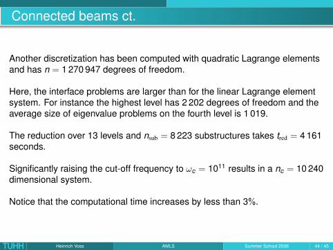
Another discretization has been computed with quadratic Lagrange elementsand has n = 1 270 947 degrees of freedom.
Here, the interface problems are larger than for the linear Lagrange elementsystem. For instance the highest level has 2 202 degrees of freedom and theaverage size of eigenvalue problems on the fourth level is 1 019.
The reduction over 13 levels and nsub = 8 223 substructures takes tred = 4 161seconds.
Significantly raising the cut-off frequency to ωc = 1011 results in a nc = 10 240dimensional system.
Notice that the computational time increases by less than 3%.
TUHH Heinrich Voss AMLS Summer School 2006 44 / 45

Connected beams ct.
Results of AMLS applied to large linear eigenvalue problems
Elements n ωc nc nsub nlevel tred
Linear 517 161 4·108 218 3 763 12 499 secLinear 517 161 4·109 613 3 763 12 502 secQuadratic 1 270 947 4·109 653 8 223 13 4 161 secQuadratic 1 270 947 1·1011 10 240 8 223 13 4 232 secLinear 1 951 170 4·109 648 13 694 14 5 431 secLinear 2 297 175 4·109 651 15 283 14 7 928 sec
TUHH Heinrich Voss AMLS Summer School 2006 45 / 45


![Solving Linear Systems: Iterative Methods and Sparse · PDF fileSolving Linear Systems: Iterative Methods and Sparse Systems ... [non-singular] matrix O(n3) LU decomposition Works](https://img.dokumen.tips/doc/110x75/5a7957ed7f8b9ac53b8d88c9/solving-linear-systems-iterative-methods-and-sparse-linear-systems-iterative.jpg)