Embed Size (px)
Citation preview

7 DESIGNING ITERATIVE LEARNING AND REPETITIVE CONTROLLERS
Richard W. Longman
Department of Mechanical Engineering
Columbia University
New York, NY 10027, USA
Abstract: This chapter discusses results in learning and repetitive control presented in a series of 60 publications. Emphasis in the summary is on the most practical approaches, with 8 learning laws discussed in detail, together with experimental demonstrations of their effectiveness. The distinction between learning control and repetitive control is discussed, and for linear systems it is suggested that in practical applications there is very little distinction, with most of the learning laws being ones that could be applied to either class of problems. Methods of long term stabilization are introduced, including use of zero-phase low-pass filtering of the error or the accumulated learning signal, and quantization based stabilization. Long term stabilization is demonstrated in experiments up to 10,000 repetitions. Learning laws are presented that require tuning only 2, 3 or 4 parameters. The methods of tuning them are clear, and can be done experimentally without needing a mathematical model. Demonstrations on a commercial robot performing a high speed maneuver, resulted in decreases in the RMS tracking error by factors of 100 to nearly 1,000 in a small number of repetitions. Such improvements can be obtained by simply tuning the learning controller in a manner similar to how one might tune a PD controller.
7.1 INTRODUCTION
long term stabilization
7.1.1 Background
This chapter gives a short overview of research in iterative learning and repetitive control by the author and co-workers, that appears in 60 publications.
Z. Bien et al (eds.)., Iterative Learning Control
© Springer Science+Business Media New York 1998
108 ITERATIVE LEARNING CONTROL
The first paper in the series, (Middleton, et al., 1985), was the result of visiting Prof. Goodwin at the University of Newcastle, Australia, in early 1984, and was submitted for publication later that year. The purpose of the visit was to determine some way in which adaptive control ideas could be used to eliminate repeating errors in robots performing repetitive tasks. But addressing adaptive based learning control methods came later, and this first paper made use of integral control concepts applied in the repetition domain, using a "p-integrator". Other independent early works with the objective of eliminating repeating errors in robots include (Arimoto et al., 1984, Casalino et al., 1984; Craig, 1984), with (Uchiyama, 1978) a precursor, as listed by Arimoto in (Longman et al., 1991). These four use a learning control formulation, resetting to the same initial condition before every new period. The Middleton paper is a robot repetitive controller, performing a periodic command. One can either consider that the desired trajectory is simply a periodic function of time and there is no resetting, or the problem is a learning control problem with resetting, and the portion of the trajectory used for resetting is included in the total trajectory to make the desired periodic command. It is very similar to such works as (Tomizuka et al., 1989), although it does not address non minimum phase zeros. Other early repetitive control publications include (Inoue et al., 1981; Omata et al., 1984; Hara et al., 1985a, 1985b; Nakano et al., 1986). The subsequent research effort reported in the 60 publications discussed here, first studied as many possible approaches to learning in repeating operations as we could think of, including methods based on integral control, indirect and direct adaptive control, numerical optimization, root finding, contraction mappings, etc. More recently, the focus is on methods that prove to be simple, practical, and effective in substantial experimental tests.
7.1.2 Research Aim - Development of Useful Practical Approaches
We summarize some of the aspects of the research effort that result from this aim to make methods that are very practical and effective.
1) Results for linear time invariant systems are emphasized: Our original motivation, and that of iterative learning control, was eliminating repeating errors in robots as they repeatedly execute a command. We develop some rather strong theoretical results for general nonlinear systems, but the majority of the references treat systems governed by linear models. This is in contrast to much of the learning control literature that is very focused on the nonlinear robot equations. The status of our linear approaches is analogous to the status of linear feedback control methods. Classical control is totally linear in its thinking, and yet in engineering practice it is often applied very successfully in nonlinear engineering problems. The linear learning and repetitive control laws developed here possess the same potential in applications, and this is demonstrated in hardware. Experiments on a commercial robot decreased the tracking error by a factor of nearly 1,000 in roughly 12 repetitions for learning. This is very close to the reproducibility level of the robot. Hence, no other method will do substantially better, and there is no need to concern oneself with

ILC DESIGNS 109
the nonlinearities of the robot dynamics in solving this real world engineering problem. And of course, in practice one uses the simplest control method that does the job, and avoiding the need for deriving the form of, and then using the large set of nonlinear robot dynamic equations is certainly simplifying.
By emphasizing linear time invariant systems, we maximize the potential for practical impact of the results. Linear systems are by far the largest class of applications for which one can make general control methods, and in the process we can often handle nonlinear problems as well. If one must take a step from linear time invariant control thinking toward nonlinear models, the next stage is to use time varying linear models. Presuming that a feedback controller is in operation, which gets one in the neighborhood of the desired trajectory, then linearization about this trajectory produces linear models with time varying coefficients, and many methods in the references also handle this class of problems, again avoiding complicated nonlinear models. The references also contain some theoretical results for fully nonlinear systems, including ones with sliding friction and stiction. These results are quite general, applying to a very large class of nonlinear systems, and are not restricted to the specific form of rigid robot equations.
2) Discrete time methods are emphasized: Implementation of learning and repetitive control must be digital, so the design of the control law might as well acknowledge this from the start.
S) We always consider that there is an existing feedback controller in operation: The learning or repetitive control simply adjusts the command to this controller in order to reduce or eliminate the tracking error. Hence, we bypass all the issues about whether to learn position or velocity, etc., and simply learn directly whatever is the variable of interest.
4) We do not create the feedback controller in conjunction with the learning control: This eliminates the characteristic of much of learning control for robots, that the method dictates the feedback control design as well as the learning control. In order to use such a method, one would have to have the robot manufacturer modify his product. It is much easier to modify the command to an existing feedback control system than it is to get a manufacturer to modify his product for use of your new promising control law.
5) We allow considerable knowledge about the system and make methods that are robust to what we do not know: The objective in much of the early work in the references, for both nonlinear and linear systems, aimed to guarantee convergence to zero tracking error for the largest possible set of systems, i.e. aimed at guaranteeing convergence with as near to no knowledge about the system as possible. There is an appeal to producing a "black box" controller that will learn to eliminate the error in any system performing a repetitive command - just connect up the wires and turn it on. On a theoretical level this objective of obtaining convergence for almost any system has obvious appeal, and might appear to maximize the usefulness of the design. Even the most basic form of learning control applied to either linear or nonlinear systems comes surprisingly close to this black box objective - on paper (Phan et al. 1988a; Longman et al., 1992b). But, of course, it is too good to be true in
110 ITERATIVE LEARNING CONTROL
us control engineers to continue to have problems to work on. In the real world, the appearance of impractically bad transients during the learning process indicates that one must pose the problem with some system knowledge in order to make learning and repetitive control laws that are of widespread practical value.
Here, we consider that it is perfectly reasonable to assume knowledge about the system equivalent to the knowledge that the feedback control system designer has. In some cases the learning or repetitive control law is designed by the same person that designs the feedback controller, and otherwise, with an existing feedback controller one can do some input-output testing, for example, to make a frequency response plot. Hence, in spite of the attractiveness of a black box learning controller, in the real world there is little need for the generality - one usually does or can easily know a great deal about the system. In addition, a byproduct of this assumption is that many of the laws developed make a good impedance match with typical control system designer thinking, and this facilitates ease of adoption of the methods.
6) We de-emphasize the issue of stability or convergence, and emphasize good learning transients: Stability, or proofs of convergence to zero tracking error are simply not sufficient for practical applications. We put the emphasis on finding ways of guaranteeing that the transients during the learning process are acceptable {some simulations of stable learning control laws on robot problems reached 1019 radians error, but they are guaranteed to converge to zero error (Chang et al., 1992)). The distinction between stability and good performance is very large for learning control. In addition, it is not obvious that we actually need convergence in many engineering problems - one can use an unstable learning process with very good results (Longman et al, 1994).
7.2 OVERVIEW OF DESIGN APPROACHES
There are various different characteristics that might be used to classify the learning and repetitive control methods developed in the 60 references. The following is a straightforward listing that contains some overlapping categories:
1) Integral Control Based Learning and Repetitive Control (Elci et al., 1994a; Fabien et al., 1995; Huang et al., 1996; Longman et al., 1990b, 1992b, 1994, 1997a; Middleton et al., 1985; Phan et al., 1988a, 1989c; Solcz et al., 1992a, 1992b, 1992c). 2) Integral Control Based with Zero Phase Low Pass Filtering (Elci et al., 1994a; Longman et al., 1997a). 3) Integral Control Based with Linear Phase Lead and Zero Phase Low Pass Filtering (Hsin et al., 1997a, 1997b; Wang et al., 1996a). 4) Integral Control Based with Linear Phase Lead and Causal Low Pass Filtering (Hsin et aI., 1997b, 1998b). 5) Integral Control Based with Compensator and Zero Phase Low Pass Filtering (Elci et al., 1994b).

ILC DESIGNS 111
6) Learning and Repetitive Control using DSP and Windowing Concepts (Wang et al., 1996a, 1996b; Hsin et al., 1997b). 7) Accumulated Signal Zero Phase Low Pass Filtering in Learning and Repetitive Control (Hsin et al., 1997b; Longman et al., 1998a). 8) Phase Cancellation Based Learning and Repetitive Control (Elci et al., 1994c; Jang et al., 1996b; Longman et al., 1996c, 1997a; Lee-Glauser et al., 1996; Hsin et al., 1997a, 1997b). 9) Learning and Repetitive Control with Model Updates (Elci et al., 1994c; Longman et al., 1996c; Lee-Glauser et al., 1996; Juang et al., 1993, 1990; Phan et al., 1995, 1989b). 10) Contraction Mapping Learning and Repetitive Control (Jang et al., 1994, 1996a; Lee-Glauser et el., 1996; Hsin et al., 1997a, 1997b; Longman et al., 1997a). 11) Finite Word Length Learning and Repetitive Control (Hsin et al., 1997b, 1998b; Longman et al. 1998a). 12) Batch Process Repetitive Control (Hsin et al., 1997a; Ryu et al., 1994a). 13) Inverse Control (Lee-Glauser et al., 1996; Longman et al., 1992a; Oh et al., 1997; Wen et al., 1998). 14) Learning Control in Nonlinear Systems (Longman et al., 1992b, 1998b; Wang et al., 1994). 15) Indirect Learning and Repetitive Control (Lee et al., 1993; Longman et al., 1992a, 1992d; Phan et al., 1989a, 1989d; Wen et al., 1997). 16) Direct Model Reference Learning and Repetitive Control (Lee et al., 1994; Phan et al., 1988b). 17) Basis Function Learning and Repetitive Control (Oh et al., 1997; Wen et al., 1998, 1997). 18) Alternating Sign Learning and Repetitive Control (Chang et al., 1992; Chang, 1993; Longman et al., 1992b, 1996a). 19) Learning in a Wave with Bounded Error (Chang et al., 1992; Chang, 1993). 20) Bisection Learning Control (Chang et al., 1992). 21) Learning to Minimize a Cost and Minimizing a Cost During Learning (Harokopos et al., 1987; Longman et al., 1989, 1990a; Li et al., 1998; Wen et al., 1998). 22) Numerical Optimization Based Learning (Longman et al., 1989; Beigi et al., 1991; Harokopos et al., 1987). 23) Numerical Root Finding Based Learning (Longman et al., 1992b; Chang, 1993; Wang et al., 1994). 24) Repetitive Control to Eliminate Periodic Measurement Disturbances (Hsin et al., 1998a). 25) Decentralized Learning and Repetitive Control (Lee et al., 1992, 1993; Longman et al., 1992a). 26) Integral Control Based Learning with Anti-Reset Windup and Other Limitations of Command Adjustments (Ryu et al., 1994b; Chang et al., 1992). 27) Learning Control Actions Computed with Transform Methods (Lee-Glauser, 1996; Elci et al., 1994c). 28) Learning Control in the Presence of Coulomb Friction and Stiction (Long-

112 ITERATIVE LEARNING CONTROL
man et aI., 1992b; Chang, 1993; Wang et aI., 1994). 29} Fuzzy Logic Gain Adjustment in Learning Control (Jang et aI., 1996a; Phan et aI., 1988a). 30} Use of unstable Learning and Repetitive Control with Learned Signal Frozen at Minimum Error Value (Longman et aI., 1994; Huang et aI., 1996). 31} Learning to Track More Output Variables than Inputs, Learning to Track Unmeasured Variables, Inter-Sample Ripple Attenuation Methods (Longman et aI., 1997a). 32} Local Learning Control (Dh et aI., 1997; Wen et al., 1998). 33} Convergence to Zero Tracking Error for Sufficiently Small Learning/Repetitive Control Gains Determined by Root Locus Departure Angle Condition (Longman et aI., 1990b).
The methods discussed in this chapter come from Items 1-12, and have been tested in experiments reported in (Elci et aI., 1994a, 1994b, 1994c; Lee-Glauser et aI., 1996; Hsin et al., 1997a, 1997b, 1998a, 1998b). Some other items are summarized in previous overview papers, (Phan et aI., 1990; Longman et al., 1992c; Longman 1995, 1996b, 1997b).
7.3 THE HARDWARE USED IN EXPERIMENTAL DEMONSTRATIONS OF ITERATIVE LEARNING AND
REPETITIVE CONTROL
7.3.1 High Precision Fast Motion Robot Tracking Using Learning Control
Learning control experiments were performed on the redundant 7 degree-offreedom Robotics Research Corporation K-Series 8071HP manipulator with Type 2 robot controller, shown in Fig. 7.1. The low level controller sample rate is 400 Hz. The closed loop bandwidths for all joints is 1.4 Hz, which is limited by the presence of the first vibration mode around 5.4 Hz. The second mode occurs somewhat above 18 Hz. Learning control is implemented on each joint in a decentralized manner. The same desired trajectory is commanded to all 7 joints, to facilitate comparisons, and consists of cycloidal paths for each joint of a 90 deg turn followed by a return to the starting point. This result is a large motion through the workspace, and the joints closest to the base reach the manufacturer's maximum speed limit. This assures a high degree of nonlinear dynamic coupling between joints, maximizing nonlinear effects to demonstrate the effectiveness of the learning control methods. Gravity disturbances prevent the feedback controllers from locating the robot end-effector on the starting points of the desired link trajectories, and therefore the initial condition is learned by extending the desired trajectory at the beginning by one second with a cycloid. Figure 7.2 shows the error produced by the robot feedback controllers (the line marked initial) in executing the commanded trajectory (the extra one second is not shown). This figure is similar for all joints. The tracking error reaches a maximum of nearly 9 deg.

ILC DESIGNS 113
7.3.2 High Precision Velocity Control in a Double Reduction Timing Belt
Drive, Using Repetitive and Batch Process Repetitive Control
The 8 to 1 double-reduction timing-belt drive system used in the experiments is shown in Fig. 7.3. Such hardware is a very common element in motion control systems. A DC motor drives the input shaft, whose gear drives a timing belt connecting to one end of an idler shaft. The other end drives a second belt which drives the output shaft. The belt teeth prevent slippage, although the belts may have some elasticity. The output shaft has a small flywheel load and an incremental encoder. An index pulse is available for once around of the output shaft and it is used to trigger each period in the repetitive control. The desired output shaft velocity is one revolution per second, or equivalently a linear tangential velocity at the output shaft radius of 0.108 m/s. A digital feedback controller with a 1000 Hz sample rate drives the input shaft using feedback from the encoder. A well designed classical controller is in operation. The bandwidth is limited to about 45 Hz, and there is no obvious way to increase this figure within classical control system design methods. The input/output frequency response reaches a phase lag of 180 degrees around 75 Hz.
Under steady operating conditions there are fluctuations in the output velocity, with the root mean square (RMS) error between 6 and 7 x 10⁻⁴ m/s. There is a rich frequency spectrum for this error as shown in Fig. 7.4, with error peaks reaching nearly to the Nyquist frequency of 500 Hz. The objective of the repetitive control is to produce high precision motion, eliminating the velocity errors from imperfections in machining or manufacture of the moving parts, and from imperfect alignment when mounting the hardware. Error sources include: 1) Shaft center of mass imbalance, 2) Shaft eccentricity with the geometric center not being aligned with the rotation axis, 3) Misalignment of the shafts, which can introduce errors at once around of the shaft and harmonics, 4) Belts also have errors at once around and harmonics, 5) Teeth meshing introduces velocity errors at the meshing frequency and harmonics, and 6) There can also be error from bearings at four distinct frequencies, the fundamental train frequency, ball spin frequency, outer race, and inner race frequency.
To interpret the rich frequency spectrum, once around errors of the output shaft, idler shaft, input shaft, input belt, and output belt produce, 1 Hz, 4 Hz, 8 Hz, 2 Hz, 2/3 Hz errors and their harmonics, respectively. In addition to these, there is output belt tooth meshing at 80 Hz, and input belt tooth meshing at 240 Hz, and we note that these produce large peaks. A period of 3 seconds is a common period for all of these errors. Note that errors from the bearings may not be consistent with this common period, and would appear as disturbances to the repetitive control system. In (Hsin et aI., 1997a), a methodology is given for hardware design for repetitive control - designing the gear sizes for a prescribed overall ratio in such a way as to minimize the common period that must be used by the repetitive controller.
114 ITERATIVE LEARNING CONTROL
7.4 A BASIC MATHEMATICAL FORMULATION OF LINEAR ITERATIVE LEARNING CONTROL
(Phan et al., 1988a) develops a general formulation for linear learning control (see also Chapter 15 in this volume). Many of the references build on the formulation developed there, and one obtains an overall perspective by viewing the various different learning control laws discussed here in terms of this formulation. Hence, we devote this section to discussing this formulation.
7.4.1 A MIMO Time-Varying State Space Formulation with Repetitive Disturbance
A multiple-input, multiple-output (MIMO) discrete-time state-variable formulation is used. Time varying coefficients are allowed, and can be used to model nonlinear systems such as robots, when linearized about the desired trajectory. Linearization produces time varying coefficients, and in addition, external forces such as gravity produce a forcing function which repeats every repetition. We usually use the state variable equations to represent a closed loop control system, e.g. a robot with its joint controllers. The input u{k) is the learning control action which is added to the the p step desired trajectory to form the command to the feedback controller. But of course, the formulation is happy to represent some open loop dynamic system, e.g. the torque applied related to the robot response. The state equations are
x{k + 1) = A{k)x{k) + B{k)u{k) + w(k) k = 0,1, ... ,p - 1
y(k) = C(k)x(k) k = 1,2, ... ,p (7.4.1)
The w(k) can contain periodic disturbances such as gravity, that appear every time the command is given, and it also contains the desired trajectory according to whatever feedback control law is being used. There is an alternative formulation where u(k) is the command, and it is also possible to use an observation equation of the form y(k) = C{k)x{k) + D{k)u{k), e.g. (Elci et al., 1994b).
7.4.2 Plug in vs. Modified Commands in Learning and Repetitive Control
The repetitive control literature sometimes talks of a plug-in repetitive controller, that taps the error signal going into an existing controller, applies its repetitive control law , and then adds the result to the controller output before it is applied to the plant. In (Middleton et al., 1985), Middleton et al. made use of this structure, but in essentially all of our other papers, we have the learning or repetitive control action modify the command to the feedback controller. Making changes in the command you give a feedback controller is likely to be very simple, but plugging in a repetitive controller may require hardware changes, or at least require going into the controller software and making modifications. (Solcz et al., 1992a), shows that the two formulations are essentially

ILC DESIGNS 115
equivalent, with possible differences being related to what signals have a zeroorder hold. We conclude that, modifying the command is to be preferred in most engineering applications.
7.4.3 State Space Formulation in the Repetition Domain
Column vectors giving the complete histories of the input and the output for repetition j are represented by '.!!j and '!lj' We use a delta operator ISj '.!! = '.!!j -'.!!j-l which is also applied to '!l (in some applications a different operator is needed, e.g. ISj = '.!!j - 1!0). When applied to (1), w(k) and the repeating initial condition (for learning control) are eliminated. Then a modern control formulation in the repetition domain is
y. = Iy. 1 + PlSj '.!! -3 -3-
(7.4.2)
Here the control variable becomes the change in control from the last repetition, and the system matrices I, P contain I the identity matrix and P which is a lower block triangular matrix containing the Markov parameters of the unit pulse responses (for the time-invariant case the entries are of the form C A i B) . From (7.4.2) it is necessary to have one input in u for every output in y for which one wants zero tracking error. By crossing out some rows of (7.4.2), one can produce zero tracking error of more output variables by not asking for zero error every time step, or by alternating which variables are addressed at successive time steps (Phan et al., 1988a, 1989cj Lee et al., 1993j Longman et al., 1997a). When one skips steps, the diagonal blocks start building the columns of the controllability matrix. Thus one can produce zero tracking error of the whole state every n time steps, where n is the order of the system. This shows us how to use under-specification to give guaranteed geometric feasibility of the chosen desired trajectory based on an upper bound on the order of the system, and the assumption of controllability. When feasibility is an issue, an alternative is to simply minimize a norm of the tracking error, as discussed in some of the references.
7.4.4 The General Linear Learning Control Law
A general linear learning control law has the form
(7.4.3)
where L is a matrix of learning control gains, and ~j = '!l* - '!lj is the difference between the desired trajectory and the current trajectory at repetition j. Combining (7.4.2) and (7.4.3) we get the error at repetition j in terms of the error at repetition j - 1, and the error at repetition zero:
(7.4.4)
116 ITERATIVE LEARNING CONTROL
Convergence to zero tracking error occurs if and only if (I - PL)i goes to the zero matrix as j goes to infinity, i.e., if and only if all of the eigenvalues of (I - P L) are less than one in magnitude
(7.4.5)
7.4.5 Four Important Properties of the Repetition Domain Formulation
1) Tracking problems in the time domain become regulator problems in the repetition domain. This is important because regulator problems are much easier problems in control theory. The option of applying linear quadratic regulator theory in the repetition domain comes immediately to mind, as is done in some of the references. 2) Time varying linear systems become repetition invariant linear systems. This is important because it allows one to treat time-varying systems with the much more powerful and complete theory associated with time invariant systems. 3) Convergence to zero tracking error in the time domain becomes asymptotic stability in the repetition domain. 4) Unknown disturbances that appear every repetition, disappear from the equations. Again, this is very important, since handling an unknown repetitive disturbance and totally eliminating its effect would otherwise be problematic.
7.4.6 The Structure of the Learning Gain Matrix for Different Learning Laws
The formulation oflinear learning control (7.4.3) is general, simply allowing one to fill up the learning gain matrix L in any way you wish. The references in this chapter use different approaches to producing the gains, and the resulting form of the matrix is as follows:
1) A diagonal L (or block diagonal in the MIMO case) produces the simplest form of learning control, integral control based learning (Phan et al., 1988a, 1989cj Longman et al., 1992bj Elci et al., 1994aj Huang et al., 1996) which just feeds back a constant times the error observed at the appropriate step in the previous repetition. Then the elements on the diagonal in (I - PL) determine the eigenvalues and stability of the learning process. 2) L can be as above, except that the non-zero diagonal is shifted toward the upper right corner of the matrix by a number of time steps, producing a linear phase lead (Wang et al., 1996aj Hsin et al., 1997a). 3) One can use two gain learning controllers with L having a diagonal and a sub diagonal (Phan et al., 1988aj Chang et al., 1992j Elci et al., 1994a). 4) L can have the form produced by a band of diagonals, but the center of the band is shifted toward the upper right in the matrix, as in linear phase lead and windowing designs (Wang et al., 1996a, 1996bj Hsin et al., 1997b, 1998b). 5) L can be upper block triangular, as in the contraction mapping designs (Jang et al., 1994, 1996aj Lee-Glauser et al., 1996; Hsin et al., 1997a, 1997b; Longman et al., 1997a).

ILC DESIGNS 117
6) L can be lower block triangular, as in the two gain designs, and some inverse control designs (Phan et aI., 1988a; Lee-Glauser et al., 1996). 7) L can be a full matrix of gains, as in the phase cancellation designs (Elci et al., 1994c; Jang et al., 1996b; Longman et aI, 1996c; Lee-Glauser et al., 1996; Longman et al., 1997a; Hsin et al., 1997a, 1997b).
7.4.7 Learning Control Law Computations Using the Transform Domain
Often the structure of the gain matrix L has the property that all upper left to lower right diagonals are composed of the same number repeated in every entry. For large matrices, this makes the product of L with the error in (7.4.3) approach a convolution sum (which may include non causal terms). Such convolutions for large matrices are more quickly computed by doing a product in the transform domain and taking an inverse transform, rather than computing (7.4.3) directly (Lee-Glauser et al., 1996; Elci et al., 1994c). There can be some "leakage" effects or end effects with this approach, but the computation time saved can be considerable.
7.5 STABILITY VERSUS GOOD PERFORMANCE
The stability condition (7.4.5) applied to integral control based learning with learning gain K establishes convergence to zero tracking error, provided the gain is sufficiently small, CB :j:. 0 and its sign is known (Phan et al., 1988a). If the C and B come from discretizing a continuous time system, then the product will not be zero. One usually does know the sign, but in case you do not, the alternating sign algorithm eliminates this requirement, see Item 18 above. Hence, convergence is essentially independent of the system dynamics which are contained in A. It is shown in (Longman et al., 1992b) that this same convergence, independent of the system dynamics, usually applies to nonlinear systems as well. But the approach can have poor transients. In the contraction mapping algorithm (Item 4 above) the condition II 1- PL 112< 1 (with the norm induced by the Euclidean norm) is used to obtain good transients with monotonic decay of the Euclidean norm of the tracking error. In (Oh et al., 1997), II 1- PL lit < 1 is used to obtain monotonic decay of the L1 norm of the tracking error. In many of the references good transients are obtained by requiring monotonic decay of the amplitudes of the steady state frequency response components of the error, by satisfying the condition
11- G(z)K<I>(z)1 < IVz = eiw /T (7.5.6)
where the WI represent all discrete frequencies from zero through the Nyquist frequency, G is the z-transfer function of the closed loop feedback control system, and <I>(z) is the transfer function of the learning control law. This condition and its relationship to the true stability boundary are discussed in (Elci et al., 1994b) and (Huang et al., 1996). When working to satisfy this condition, it is often convenient to use a Nyquist plot of the imaginary part and real part

118 ITERATIVE LEARNING CONTROL
of the frequency response of GK~. Equation (7.5.6) says that any frequency for which this plot is outside the unit circle centered at +1, is a frequency for which steady state amplitudes grow with repetitions. And the radial distance from +1 to any point on the plot is the multiplicative factor by which the amplitude changes each repetition for the frequency associated with that point. In learning control the fact that these amplitudes grow does not indicate instability, because the stability boundary is determined by a different convergence mechanism (Huang et al., 1996; Chang et al., 1992).
7.6 LEARNING CONTROL VERSUS REPETITIVE CONTROL
7.6.1 Steady-State Batch-Process Repetitive Control- A Bridge Between
Learning and Repetitive Control
One may ask the question, will linear learning control laws work on repetitive control problems, and vice versa? One can create a batch process repetitive control concept to facilitate this, forming a bridge between learning and repetitive control (Ryu et al., 1994a; Hsin et al., 1997a). In repetitive control we can apply a learning/repetitive control signal without updating for long enough to obtain steady state response. An updated signal is computed from this steady state data, and when available is applied at the start of the next repetition or period. This procedure converts the repetitive control problem to something as close as possible to the learning control problem. But it is not identical because the initial conditions for the different applications of the learning control law are not the same.
Batch processing has the important advantage that there is no real-time computation limitation - the repetitive control law can be as complicated as needed. Another advantage is that the repetitive control law need not be "causal" which allows use of non causal filtering, for example, a zero-phase Butterworth lowpass filter. Furthermore, it can allows efficient computation of the control action using transform methods, which can avoid the need for truncation of learning gains in a real time implementation, with possible effects on long term stability. Convergence conditions for this steady-state batch-process repetitive control approach, as well as modern state variable repetition domain equations, are given in (Hsin et al., 1997a). The same reference gives experimental results of steady-state batch-process repetitive control, using contraction mapping learning, phase cancellation learning, and integral control based learning with linear phase lead and zero phase low pass filtering (Items 10,8.3). We note that because we are always dealing with steady state behavior, the steady state frequency response convergence condition (7.5.6) is now the true stability boundary.
Note that (Wen et al., 1998) develops another type of bridge between iterative learning and repetitive control, by using basis functions. These functions allow one to extrapolate the different initial conditions that apply to each repetition without needing to explicitly write the dependence on the final values

ILC DESIGNS 119
of the previous period. This results in mathematical equations for repetitive control that are identical in form to those of learning control.
7.6.2 On the Distinction (or Lack of Distinction) Between Linear Learning
and Repetitive Control
The literature for learning and repetitive control tends to be very different. This is partly because of the emphasis on the robot nonlinear dynamic equations in learning control. For linear systems, it is also because of the apparent disparity in the stability conditions, the stability boundary for learning control being so different from that of repetitive control, as discussed in (Huang et aI., 1996). We suggest that this distinction in stability boundary is not important in most engineering applications. In order for learning control to be practical, one needs reasonable transients for the learning process. This suggests that in addition to asking for stability according to (7.4.5), one also is likely to ask for satisfaction of the more restrictive condition (7.5.6). Once one decides to require satisfaction of (7.5.6), then stability is assured whether it is a learning control problem or a repetitive control problem. Condition (7.5.6) is a sufficient condition for stability in either case (Elci et al., 1994b; Huang et aI., 1996). One might think that the alternative of satisfying the L2 norm condition for monotonic decay of the Euclidean norm of the error might be an independent condition, but it becomes identical to this frequency response condition (7.5.6) when the trajectory becomes sufficiently long (Jang et aI., 1996b).
We conclude that in practical applications of learning control to linear systems, one is likely to want to satisfy the same stability condition one would be satisfying in repetitive control. Hence, the distinction between learning and repetitive control in linear systems becomes much less significant than one would initially think. Whatever works well for repetitive control should work well in learning control. And those types of learning control that converge to zero tracking error which do not satisfy (7.5.6) or the monotonic error decay condition are likely to have bad transients that make them unattractive or impractical in applications. The main distinction is the real time computation requirement in repetitive control, and using the batch process updating discussed above, this distinction can disappear.
7.7 EIGHT LEARNING / REPETITIVE CONTROL LAWS - AND THEIR PERFORMANCE IN THE REAL WORLD
We prefer that the learning or repetitive control approaches be easily applied, and in some ways similar to routine design of feedback controllers. This makes an important impedance match with the practicing control engineer's ways of thinking, and allows him to understand and make use of the methods quickly and easily. Attention is given to methods involving only a few design parameters that can be tuned experimentally as in a PD or PID controller. We consider it reasonable to use experimental closed loop Bode plots in tuning the learning/repetitive control laws. Note that the interaction between the feedback and

120 ITERATIVE LEARNING CONTROL
learning or repetitive controller design processes is not very critical - most any feedback control system's performance can be improved very substantially and very easily by these methods. Many of the designs involve alternative methods of compensating the system to keep the above described Nyquist plot inside the unit circle centered at + 1 up to as high a frequency as possible, coupled with alternative approaches to cutting off the frequencies that go outside.
7.7.1 CONTROL LAW 1: Integral Control Based Learning with Zero-Phase
Low-Pass Filtering
Integral control based learning control is the simplest form of learning control. One can think of it as follows: when the robot link angle was too low by 2 degrees last repetition at a certain time step, add a learning gain times 2 degrees to the command this repetition at the time step that controls this error. Mathematically, this algorithm converges to zero tracking error for a very large class of systems. The convergence mechanism is one that progresses with repetitions in a wave from the start of the trajectory. What happens to that part of the trajectory before the wave arrives is irrelevant to convergence. There can easily be some higher frequency component of the error that is at a frequency that has a 180 deg phase shift going through the closed loop system. This is equivalent to changing the sign of the corrective action which adds to the error in front of this wave. The result can be very poor transients during learning. Here we introducing zero-phase Butterworth low-pass filtering to address this problem, and show that it makes this method into something totally practical, and very simple. The filtering is done on the error, but it can be done on the accumulated learning signal (without the desired trajectory included) for long term stabilization.
la) The benefit of the zero-phase low-pass filter: When we used pure integral control based learning in the robot experiments, without introducing a zero-phase low-pass filter, the error was reduced by a factor of more than 50 in 10 repetitions, before the poor transient started the error growing. The experiments could not be continued past repetition 14 because the robot was making so much noise that we were afraid of damaging it. Simulations suggest that the growth would continue (in a linear model) to roughly 1011 radians before the fact that the learning control law is stable becomes evident! This is what we call poor learning transients in a learning controller with guaranteed convergence to zero tracking error. The learning gain was 1, and convergence is guaranteed up to about a gain of 90. The cause of this type of behavior is explained in several ways in (Huang et al., 1996).
Then we introduce a 5th order zero-phase Butterworth filter with cutoff at 3 Hz. The root mean square of the tracking error was decreased by a factor of 100 in approximately 6 iterations. The RMS error history vs. repetition number is given in the first figure of Chapter 15 of this book. Repetition 0 is feedback control alone, and we see that the feedback alone RMS tracking error is somewhere between 5 and 6 degrees, corresponding to the 9 degree maximum error in Fig. 7.2. Figure 7.2 also gives the tracking error histories for the first

ILC DESIGNS 121
few repetitions, and Fig. 7.5 shows the error at repetition 6. Note that the error at repetition 6 is far too small to be visible in Fig. 7.2.
1 b) The usefulness of the algorithm in engineering practice: The above highlights how the low pass filtering has made integral control based learning into a well behaved and practical algorithm. After picking a Butterworth filter order, one has only two parameters to choose: the learning gain, and the cutoff frequency. They could be tuned purely in hardware, using one's knowledge of how they interact to make adjustments until one gets good performance. Or one can use Bode plot data as described below. A factor of 100 improvement in tracking performance for so little effort is impressive, and we suggest that this method should see many engineering applications in the future. The same methods can be applied in repetitive control with either batch process repetitive control (Item 12) or batch process zero-phase filtering in real-time repetitive control (Item 7).
lc) How to tune the two parameters - Making the gain vs. bandwidth tradeoff: Given Bode plot data that you trust, then the following procedure used for (Ryu et al., 1994a) tells you the needed cutoff frequency as a function of the learning gain. Write ~(exp(iwT))G(exp(iwT)) = N(w)exp(i8(w)) where N(w) and 8(w) are the amplitude and phase angle of the closed loop system frequency response times the learning law without the gain K, i.e. ~(z) = z. After substitution into (7.5.6), the value of learning gain K that produces unity, satisfies (1- KN cos 8)2 + (KN sin 8)2 = 1, and is given by K = 2 cos8(w)JN(w). Figure 7.6 plots this experimentally determined function for the double reduction timing belt drive system. To use the plot, you can pick a desired cutoff frequency, and then read off the maximum allowed learning gain for that cutoff (which must be positive). Since a Butterworth low pass filter is not an instantaneous cutoff at the desired frequency, one would put in a margin to allow sufficient attenuation at cutoff. Reading the other direction in the figure, one can pick the learning gain, and read the needed cutoff. Smaller learning gains take somewhat longer to learn, but are beneficial when one approaches the noise floor in the learning process, generally producing somewhat smaller final error levels in the presence of random noise (Phan et al., 1988a), and also having smaller error levels because of the higher cutoff frequency allowed.
ld) Automatic tuning algorithms: Alternatives to this design process are: adjust the gains empirically, or automate the adjustment as part of the learning law. If the cutoff is low enough, then the system should produce monotonic convergence. Stated another way, if the response stops exhibiting monotonic decay, then one should lower the cutoff frequency, and either start again, or do zero-phase low pass filtering of the accumulated learning signal to eliminate whatever growth has occurred. This defines rather clearly how one empirically adjusts the two parameters, and how one can pick a set of rules to follow in adjusting the parameters without needing a control system designer's expertise. It further indicates how one can make the learning or repetitive control law do the adjustment automatically during the learning process.
122 ITERATIVE LEARNING CONTROL
7.7.2 CONTROL LAW 2: Integral Control based Learning with Linear
Phase Lead and Zero-Phase Low-Pass Filtering
This learning law (Hsin et al., 1997a) is the same as that used above, except that we include a linear phase lead (Wang et aI., 1996a) to keep the Nyquist plot inside the unit circle centered at + 1 up to higher frequencies. This is a very simple form of compensator. The method above in 1) has two parameters to pick, the gain and the cutoff, and now we have three parameters to tune, the number of time steps of phase lead being the new parameter.
The batch process repetitive control action at time step k of batch repetition j, is given by uj(k) = uj-l(k) + K!(ej-l(k + 1 + 7)) where 7 is the number of time steps advance used, which produces a linear phase lead, K is the scalar learning gain, and the! indicates the zero-phase filtering operation. We apply this batch process repetitive control law to the double reduction timing belt drive system, with the learning gain set to 1/2, and the advance set to 7 = 6 time steps. A tenth order Butterworth filter with a cut-off frequency of 120 Hz is used. To set the number of time steps phase lead, we can use the same technique as above. One would make the same plot as Fig. 7.6 for each different choice of lead (picking ~(z) as different powers of z), and pick whichever gives the best tradeoff between gain and cutoff. Again, automated adjustment can also be considered.
The advantage of this control law is evident by the cutoff of 120 Hz, as compared to the cutoff limit of well under 40 Hz for Control Law 1 as seen in Fig. 7.6. This produces far superior cancellation of the errors in Fig. 7.4. Figure 7.7 gives the Nyquist plot of the feedback control system input-output relationship, which very obviously goes outside the unit circle, and with unity learning gain the cutoff is chosen to eliminate frequencies outside the circle. Figure 7.8 gives the Nyquist plot with the present repetitive control law included, and one cannot see to graphical accuracy that the curve goes outside the unit circle, but it does somewhat above 120 Hz.
Figure 7.9 gives the RMS errors for each repetition as a function of the repetition number. It only takes a few repetitions to reach the final error level. The decrease in error is not as dramatic as in the case of the robot. What determines the ultimate limit on the error that can be eliminated is the repeatability level of the system. The frequency content of the error at repetition 50 is very similar to that of Fig. 7.11 of the next section except that there is an error peak around 160 Hz that is about half the size of the peak at 240 Hz. The control law has eliminated all peaks up to its cutoff of 120 Hz.
We feel that this learning/repetitive control law may perhaps be the most useful of the designs considered. It does not produce the best error levels, but it is easy to apply, and can be tuned experimentally without modeling the system, or tuned using experimental Bode plots, and it results in essentially perfect behavior up to a cutoff of 120 Hz. It has all of the advantages of the law above, and it obtains zero tacking error up to a higher frequency. The price paid for this, is the need to adjust one more parameter.

ILC DESIGNS 123
One can make an analogy with PD controllers that require tuning two parameters as in Control Law 1, and PID controllers that require tuning three, as in the present control law. However, the tradeoffs in tuning the three parameters here are much easier to make than the associated tuning problem for PID controllers. One simply makes Fig. 7.6 with the various choices of time steps for lead.
7.7.3 CONTROL LAW 3: Integral Control Based, Linear Phase Lead with
Non-Zero Phase Low-Pass Filtering, Finite Word Length Stabilized
Control Law 2 uses a zero phase low pass filter which requires filtering both forward and backward in time through a repetition of data. This cannot be done in real time, although one can do such computations on-line, with batch updates of the repetitive control signal when the computations are ready (Hsin et al., 1997b, 1998b). An alternative to batch updates, is to no longer use a zero phase filter. Here we use an 18th order Butterworth low pass filter in real time applied to the error. The cutoff is 160 Hz and the learning gain is 0.5. The phase lag it produces adds to the phase lag of the system, to produce the total phase lag that a linear phase lead (now 19 time steps) is chosen to cancel in such a way as to keep the Nyquist plot inside the unit circle up to as high a frequency as possible. In (Hsin et al., 1998b) we make the claim that most repetitive controllers are unstable if you wait long enough. This was stated partly for shock value, and partly because it is likely to be true. The results of using a 12th order Butterworth, rather than the 18th order used here, produces an RMS error plot similar to Fig. 7.9, but it continues to repetition 1,000. Most experimentalists would be quite satisfied with such results, showing 1,000 repetitions of good behavior. But the instabilities in these designs can be very slow instabilities. When the same 12th order law was run longer, an instability started to appear around 2,600 repetitions, Fig. 7.10 (the step discontinuities every 1,000 repetitions are due to having to restart the experiment due to storage limitations). The 18th order result is stabilized by finite word length in the computer. In (Hsin et al. 1998b), methods are given to pick a quantization level that will stabilize learning and repetitive control laws, and could be used to stabilize the 12th order case. Figure 7.11 shows a simulation of how a quantization level of 10-5 stabilizes pure integral control based learning on the robot. The method predicts stability of the 18th order case using the 7 digits of accuracy in the computer, and experiments were run to repetition 10,000 as shown in Fig.7.12.
This repetitive (or learning) control law uses 4 design parameters: the learning gain, the cutoff frequency, the number of time steps lead, and the quantization level. One can use the procedure for picking the needed quantization level given in (Hsin et al., 1998b), or one can simply adjust it experimentally (using long experiments!).

124 ITERATIVE LEARNING CONTROL
7.7.4 CONTROL LAW 4: Linear Phase Lead with Triangular Windowing,
Finite Word Length Stabilized
This repetitive (or learning) control law uses a triangular window or Bartlett window in place of the Butterworth filter of Control Laws 1 and 2 (Wang et al., 1996a, 1996b: Hsin et al., 1997b). The window can have zero phase change, so the linear phase lead is used only to cancel as well as possible the phase lag of the feedback control system. The window is simply a triangular moving average, so that it is a simpler computation than solving the Butterworth difference equations, but this simplicity is at the expense of the window being further from an ideal low pass filter. Again the learning law has 4 parameters to choose, the learning gain (here it is 0.5), the linear phase lead (6 time steps), the width of the triangular window which determines the cutoff frequency (a width of 13 time steps was used for a cutoff of the main lobe in the frequency response of the filter at approximately 150 Hz), and the quantization level. Again, no explicit quantization level was introduced in the experiments, but the digital control implementation used 7 significant digits for word length. Experiments were run for 1,600 repetitions, and the error spectrum at the end is rather uniform throughout the whole 500 Hz range, containing small peaks throughout, see (Hsin et al., 1998b). We see that the method does not eliminate the errors below its cutoff as well as the previous method, and it does attenuate some of the peaks above the cutoff. The method does not have as good performance as other methods above, but the window is particularly simple, and can be applied in situations where it allows one to meet on-line computation constraints.
7.7.5 CONTROL LAW 5: Two Gain Learning with Zero-Phase Low Pass
Filtering
Below equation (7.4.3) there is a discussion of the structure of the learning control matrix. The emphasis in (Phan et al., 1988a) was on lower triangular matrices (or block lower triangular for MIMO). This structure preserves the eigenvalues of (I - PL) as 1 - CBK1 where K1 is the gain along the diagonal of L. In spite of the large size of the matrix, we know the eigenvalues easily in terms of Band C because of the lower triangular structure, and can ensure stability of the learning process easily using a sufficiently small diagonal learning gain. Then, one wonders how can we pick the rest of the gains to fill the lower triangular matrix, and obtain some benefit. One option is to use a matrix L that has K1 along the diagonal, and K2 along the sub diagonal, and the rest of the elements zero (Phan et al., 1988a; Chang et al., 1992). Suppose we know CB and CAB, for example, by putting a unit pulse input into the feedback control system, and watching the response for two steps, or by using a rich input and using OKID (Juang et al., 1993; Phan et al., 1995). Suppose that we have state feedback so that C is the identity matrix, and pick K1 = B-1 and K2 = _B- 1 A. This choice makes the sub diagonal in (I - PL) equal to zero. This happens to make all of the elements below the diagonal zero as well, in the state feedback case. Hence, it is the inverse of P.
ILC DESIGNS 125
Robot experiments using this control law are reported in (Elci et al., 1994a), and the RMS error vs. repetition curve is shown in the second figure of Chapter 15 in this volume, which is to be compared to the first figure of the same reference. We see that the use of two gains has caused the learning to be faster, converging to the final error level at about repetition 3 when it took until about repetition 6 for the single gain learning control of Control Law 1. Both use the same 3 Hz cutoff. Also, the RMS error after reaching the final error levels is more consistent with less fluctuation using this two gain learning controller.
The robot is not a state feedback system. However, the feedback controllers for each joint are designed to have a bandwidth of 1.4 Hz, so that the controller will not excessively excite the first vibration mode at about 5.4 Hz. When using OKID on rich large motion data in order to identify a model of the input-output relationship for each joint, it is only the first order pole producing the break for this bandwidth limit that is identifiable. This is likely to be the case in many robot systems. Hence, in this experiment we are using the best model we were able to get from our data, and using an inverse system learning controller. The fact that this model is a first order model means that we are using state feedback. This does not sound like a very general situation, but the comment that typical robot controllers will have such a bandwidth limit, makes the situation apply often in robotics.
The fact that an inverse model is used for the first repetition illustrates a point. At repetition 1 we are finished using the inverse of the model that we could easily obtain from some prior test. And the error level has been substantially decreased, by perhaps a factor of 10. Then we keep our learning control going and we further decrease the error by another factor of 10 in the next two repetitions (and if we instead used one of the learning controllers given below, we can continue learning and take out almost another factor of 100). Hence, this illustrates the point, that we can use the best inverse model we know, and when done, if we use a learning controller, we are likely to take significantly more error out.
So what has the effort of obtaining an inverse model bought us? The main benefit is that we get to the final error level in about 3 repetitions instead of 6. This benefit may not be worth the effort. Generally, the amount of time and effort needed to perform 3 more repetitions will be much less than the effort expended in trying to get an accurate model of the system to use for inversion. Another implication is that using an inverse model only is not enough, and one needs learning control to get to really small error levels. Note that the model here is unusual, it is first order and a well behaved inverse exists. With higher order models we are likely to experience troubles taking the inverse, making it even less useful to consider using an inverse model in place of learning or repetitive control.
In (Lee-Glauser et al., 1996) inverses of P were computed as well as possible using as large a P as we could successfully invert. The same behavior occurred that we could use the inverse model for 2 or 3 repetitions having the error decrease, and decrease faster than other learning control laws. But in that reference unlike here, we could not continue to use the inverse model learning
126 ITERATIVE LEARNING CONTROL
controller without producing quick divergence. As a result, the reference suggests starting with an inverse model learning process for these first 2 or three repetitions, and then switching to other learning laws that are better behaved (Fig. 7.15 given below does this). Inverse models in basis function space can be somewhat better behaved, and they are used in (Wen et al., 1998).
7.7.6 CONTROL LAW 6: Frequency based or Pole Cancellation based
Compensation with Zero-Phase Low Pass Filtering
Classical control system designers often design compensators. Here we consider designing a compensator, and of course the only objective is to keep the Nyquist plot inside the unit circle up to higher frequencies (although keeping it closer to the point + 1 will increase the learning rate). Compensator design in this situation is much simpler than in feedback control. The linear phase leads used above are simple forms of compensators.
In (Elci et al. 1994b), robot experimental results are given. The compensator used here was somewhat arbitrarily chosen as the reciprocal of the discretized version of a transfer function with two resonant poles matching the robot first vibration mode, and DC gain of unity. Thus, we are doing pole zero cancellation of the resonant poles, but not the first order pole defining the closed loop bandwidth of the feedback controller - a partial inverse of the system. This allows us to keep the Nyquist plot within the unit circle up past our chosen cutoff of 18 Hz, somewhat before the second resonance of the robot.
The RMS error vs. repetition number is very similar to the first figure of Chapter 15, except that there is an extra factor of 10 on the vertical axis. Use of this compensator has produced a total reduction in the RMS error that approaches a factor of 1,000, three orders of magnitude. Somewhere between 12 and 16 repetitions is sufficient to reach this error level, which is very close to the repeatability level of the robot, as assessed by conducting experiments that repeat the same command many times in succession and taking statistics on the results. On the other hand, this error level is substantially below the repeatability level assessed by conducting experiments that repeat the same command many times, but doing each test on a different day. Thus, to reach these low error levels, one cannot just use the learned signal from today when running the robot tomorrow, one must learn tomorrow again, or keep the learning process going if it is long term stabilized.
The tracking error at repetition 20 is given in Fig. 7.13, which is to be compared to Fig. 7.5 for the pure integral control based learning with a zerophase low-pass filter cutting off at 3 Hz. The tracking error looks to the eye to be close to white noise, meaning most of the deterministic error has been removed.
7.7.7 CONTROL LAW 7: Contraction Mapping Learning and Repetitive
Control
ILC DESIGNS 127
Unlike most of the previous learning or repetitive control laws which were based on (7.5.6) for their good transients, this law is based on keeping II I -PL 112< 1. The law is L = KpT where K is a learning gain (Jang et al., 1994, 1996a). This law has some important advantages in terms of robustness of the good transients, and some disadvantages in terms of speed of learning at high frequencies.
7a) Good transients: IT the P used in the control law is the true P matrix for the system, then we have monotonic decay of the Euclidean norm of the tracking errors with repetitions for all sufficiently small gains satisfying 0 < K < 2/ II p II~ where the norm is the maximum singular value of P. Then matrix I - P L is a contraction mapping.
7b) Good transients in short trajectories: When using the steady state frequency response condition (7.5.6) to obtain good learning transients, one must have a trajectory that is long enough relative to the system settling time that steady state response thinking applies. The control law here gets monotonic decay of the error norm, independent of the length of the trajectory.
7c) Robustness of the good transients: Let matrix E represent the error in the P used in the learning control law, i.e. the P used minus the true P. By making the learning gain K sufficiently small, monotonic error decay is maintained for any error matrix E. For monotonic decay K must satisfy o <II E 112< [1+ II I - KPpT 112] / [K II P 112]. Since the numerator on the right is greater than or equal to unity, and the denominator can be made arbitrarily small by decreasing the learning gain, one can in theory tolerate any amount of model error (Jang et al., 1996a).
7d) No cutoff: The approach does not use any low pass filter that cuts off the learning above some frequency. In theory, the approach obtains zero tracking error for all frequencies.
7e) Time varying and MIMO systems: Note that the algorithm is applicable to time varying (with the same time variation every repetition) as well as time invariant systems, and applies equally well to MIMO systems.
7f) Possible adjustments during learning: As with the phase cancellation algorithm below, the fact that we know we should have monotonic decay, allows us to consider algorithms that monitor the Euclidean norm of the error, and when it does not decay monotonically (for a long enough number of repetitions that noise is not the cause), we can adjust the learning gain, and/or use the current data in identification to improve the gains. Fuzzy logic adjustment of the learning gains is studied in (Jang et al., 1996a).
7g) How to find P: The entries in P are the Markov parameters, i.e. the unit pulse response time history at sample times. One could make a unit pulse test, but it would be difficult to get a large number of the Markov parameters accurately this way. One can use a long rich input such as a white noise input and then use OKID from (Juang et al., 1993), see also (Phan et al., 1989b, 1995), and (Juang et al., 1990). This algorithm is available from NASA through Cosmic. It first finds the Markov parameters of a filter, under appropriate conditions it is a Kalman filter, and from these finds the Markov parameters of the system (and in the process it produces a system model, and the Kalman
128 ITERATIVE LEARNING CONTROL
gain directly from data}. An alternative is to use the same tests, perhaps altered to help address leakage issues, and take the discrete Fourier transforms of the inputs and the outputs, take the ratio of the transform of the output over that of the input, and take the inverse transform of the result.
7h) Steepest descent interpretation: One way to derive the contraction mapping control law is to say at any time step k in a repetition, I would like to choose the change in command in such a way as to minimize the sum of the squares of all future tracking errors. This is unlike integral control based learning that only looks at the next time step in choosing its control action. The algorithm takes a step of size K in the steepest descent direction, toward minimizing this objective function.
7i) The structure of learning matrix L: This control law uses an upper (block) triangular L. This is in contrast to using the inverse of the system, p-l, which produces a lower triangular matrix. In a sense, one looks forward in time and the other looks backward in time.
7j) Handling the gains: This control law uses a large number of gains, enough to fill the upper half of matrix L (or the full matrix in the case of steady-state batch-process applications, Hsin et al., 1997a). Thus, it makes a good candidate for use of transform methods. Another alternative is to recognize that the pulse response of an asymptotically stable system will decay with time, making the Markov parameters get small. One can consider cutting them off when they become what one considers negligible. When the gains are truncated it is possible that the process introduces phase distortions and side lobes that affect convergence, and in theory would require a decrease in learning gain to maintain robustness. No such difficulties were observed in the experiments.
7k) Slow learning at high frequencies: We can convert the law to the 7r
domain in order to study the frequency response characteristics (Jang et al., 1996a). The transform of the learning law and the feedback control system can be written in terms of the Markov parameters, making use of their physical meaning, L(z) = K(CBz + CABz2 + ... ) and G(z) = CBZ-l + CABz-2 + .... Then the Nyquist plot corresponding to G(z)K~(z), becomes a plot of
(7.7.7)
Hence, this learning law makes the entire plot lie on the positive real axis, with gain K adjustable to keep it inside the unit circle centered at + 1 for all frequencies. This is its most important advantage. A disadvantage according to (7.7.7) is that the learning rate dies with frequency as the square of the decay in output of the feedback controller. This low learning rate at high frequencies may underlie the property observed in the robot experiments using this learning law (Lee-Glauser et al., 1996), that the final error levels reached in Fig. 7.14 are not as good as those for Control Laws 6 and 8 ..
7l)Modi/ications of the high frequency learning rote: One can modify the control law by replacing its P by its singular value decomposition with the singular values modified as desired to change the learning rate (Jang et al., 1994). Of course, the need for a decomposition of a large matrix makes such

ILC DESIGNS 129
an approach less desirable. But, as the matrix gets large, the singular values approach correspondence with the discrete frequencies, so that one is adjusting the frequency response. (Jang et al., 1996b) does this, using a partial isometry, replacing all singular values by unity, to develop a time domain form of Control Law 8 starting with this contraction mapping algorithm.
7m) Use in steady-state batch-process repetitive control: Hsin et al. (1997a) proves that the same monotonic decay of the Euclidean norm of the error for sufficiently small gains K applies to steady-state batch-process use of this algorithm, as does the robustness to inaccuracies in the P in the control law. Note that the matrix P now takes on a rather new form, no longer lower block triangular. Experiments on the double reduction timing belt drive system were performed with a gain of K = 1/2. The control action could have been calculated in the transform domain, but here it was done in the time domain. A full implementation would require use of 3000 gains every time step. These were truncated to the first 200. The RMS error plot decays more slowly than that in Fig. 7.9 reaching the final error level around batch repetition number 25 to 30. The final error level is similar to that in Fig. 7.9 but somewhat smoother with repetitions. The frequency content at repetition 50 is similar to Fig. 7.12 except that the 160 Hz peak remains, as well as some small peaks below 160 Hz. The contraction mapping law does not have a cutoff and in theory should eliminate all peaks. The slow learning at high frequencies can decrease signals below the word length of the computer and prevent the corrective action from accumulating the needed signal. In summary, we obtain substantial robustness, but at the expense of some performance.
7n) Real-time repetitive control: The proofs of monotonic decay and robustness of good transients do not apply when implemented in real-time repetitive control. Experiments could use only 60 Markov parameter gains, due to computation limitations at the 1000 Hz sample rate. Figure 7.15 shows the error spectrum at repetition 1000. The slightly increased amplitudes at high frequencies suggests that there will be long term stability problems with the approach. The robustness and long term stability were the main advantages of the approach, and one pays for these advantages with decreased performance. Therefore we suggest restricting use of the method to the learning and batch process repetitive control situations.
7.7.8 CONTROL LAW 8. Phase Cancellation Learning and Repetitive
Control with Identification Updates
The use of a zero-phase low-pass filter in many of the learning and repetitive control algorithms above simply tries to stop the learning action at high frequencies, and not attempt to learn them. The contraction mapping is mathematically shown to converge for all frequencies, but it learns high frequencies very slowly. In the phase cancellation design here, we will again try to learn all frequencies, but this time we use re-identification as our means of producing long term stabilization. Of course, we could also cut out high frequency components that start to grow using our present system model, rather than

130 ITERATIVE LEARNING CONTROL
improve the model, so that they do not grow. Elci et al. (1994c) creates the algorithm and tests it on the robot, as does (Lee-Glauser et al., 1996). Hsin et al. (1997a, 1997b) apply the algorithm in batch process repetitive control and real time repetitive control, respectively. Longman et al. (1996c) discusses model updating in the frequency domain directly, and Longman et al. (1997a) discusses ways of making the algorithm learn more output variables than input variable, or attenuate ripple between sample times, etc.
8a) Phase cancellation is a partial inverse approach: The inverse is in the phase of the steady state frequency response model. The rule used here aims at making ()(z) supply a phase change that cancels the phase change of the feedback controller in G{z), and makes no change in amplitude {except in the case of peaks of the frequency response which in (Elci et al., 1994a) are attenuated to an overall gain of unity). Therefore, the amount of learning each repetition decays with frequency like the decay in the magnitude Bode plot of the feedback controller. The contraction mapping decayed like the square of this rate, and that mathematically appears to be sufficiently slowly that we have a long term robustness result. Using the slower decay with frequency of the phase cancellation algorithm, we do not have this robustness for reasonable gain levels, and re-identification or elimination of frequencies is necessary. The decision not to make changes in the amplitude as a function of frequency in choice of ()(z) is somewhat arbitrary. We can, of course, make any change we desire. It was felt that this choice is a good compromise between the learning rate at high frequency, and the model inaccuracies one expects at high frequencies.
8b) Implementation in either the frequency domain or the time domain: There are at least three ways to perform the controller computations. (i) FFT computations: Given a system model, we know what phase lead (lag) to supply at each discrete frequency to cancel the phase lag (lead) of the feedback controller. After each repetition we take the FFT of the error history, change the phase of each frequency component as needed, and then we take the inverse transform to obtain the time history of the next control action. (ii) Convolution sum: The computation above is a product of something that changes phase and not amplitude (except for reducing peaks above unity), multiplied by the FFT of the error. The inverse transform of this product in transform space is a convolution sum in the time domain, which can be written as a sum of gains times error components. So one can simply use these gains in the time domain. Note that one will truncate the gains to some reasonable number. Both the frequency computation above and this computation that comes from the frequency domain back to the time domain, require sufficiently long trajectories that steady state frequency response thinking is applicable. (iii) Short time trajectory gains: For shorter trajectories, the partial isometry learning law below is a totally time domain approach to obtaining the needed gains.
8c) MIMO version of the algorithm: If we assume that the feedback system square frequency transfer function matrix can be diagonalized at each discrete frequency WI, G{z) = V-1{z)A{z)V{z), z = exp{iwIT), then we can write the learning control law frequency domain components as
ILC DESIGNS 131
~(exp(iWIT)) = V-l(exp(iwIT))A~(I)V(exp(iwIT)) (7.7.8)
where A is the matrix of eigenvalues, A~ is a diagonal matrix of the eigenvalues with the signs of their phases reversed, and their amplitudes set to unity (or one over the amplitude for frequencies that are amplified).
8d) The contraction mapping learning is a phase cancellation law with attenuation: When using the contraction mapping algorithm, the product P L = K P pT is like a zero phase low pass filter, the p filtering forward in time, and the pT filtering backward in time. And, of course this squares the attenuation (or amplification) at the same time that it produces zero phase. So it is a phase cancellation algorithm, but with amplitude attenuation included. Instead of using a zero-phase low-pass filter and a compensator, the contraction mapping algorithm uses pT to accomplish both tasks. To convert the contraction mapping algorithm to the present phase cancellation algorithm we need to eliminate the attenuation in the learning law, as is done next.
8e) Learning control using a partial isometry - a finite time version of phase cancellation, done totally in the time domain: To eliminate the amplitude changes in the contraction mapping learning law, use the singular value decomposition P = UEVT. Since matrices U, V are unitary, all attenuation or amplification is contained in the diagonal matrix of singular values E. We simply remove this matrix from the control law, which becomes L = K(UVT)T = KVUT (Jang et al., 1996b). (Writing p = UEVT = (UEUT)(UVT), the first factor is a real symmetric and positive definite matrix, and the second factor is a partial isometry, whose transpose is in the control law.) Obviously the attenuation of G~ (i.e. PL) with frequency will be the same as that of P, since the learning law L does not attenuate. Thus, this forms a direct time domain way of computing the phase cancellation learning control law.
This approach has the advantage that there is no requirement for having a sufficiently long trajectory that steady-state frequency-response thinking can apply. Hence, it is to be preferred in situations where the trajectory is short, i.e. when the settling time is a substantial part of the time for one repetition. Note that the frequency response based approach to phase cancellation produces a set of gains that are the same ones used every time step, when converted to the time domain. The computation here does not do this. For a sufficiently long trajectory, the middle of the matrix will have these same gains each time step, but there will be differences in the early and late parts of the matrix. Hence, the frequency response approach gets the answer for large matrices, theoretically infinite matrices, and the solution here is the correct answer for finite size matrices. An implication of this, is that one cannot use transform methods to implement this finite time version of the control law.
Note also, that this thinking connects two good learning transient conditions, the contraction mapping of the Euclidean norm of the error, and the monotonic decay of steady state amplitudes for all frequencies, equation (7.5.6). Many above approaches use filtering adjusted using steady state frequency response thinking. These same approaches can now be extended to the finite
132 ITERATIVE LEARNING CONTROL
time equivalent, using the match between singular values of P and the discrete frequencies. One adjusts the singular values as one would the corresponding frequencies in designing the filter, producing finite time "low pass filtering" in the singular value space for short trajectories.
8f) Long term stabilization - choices in the re-identification approach: (i) In the re-identification done in the robot experiments, a modern control realization was obtained using OKID and ERA-DC (Juang et aI., 1993), and from this model the phase angle vs. frequency information was obtained. (ii) Longman et al. (1996c) uses identification directly in the frequency domain, without going through a model. One simply uses transforms of the inputs and outputs to decide the phase change. Certain rules were constructed to handle many of the subtleties of system identification, in order to assure improvements from the identification updates. (iii) When one is using P to form the control law, as in (Jang et aI., 1994), one can: (a) use the modern control realization matrices to compute the Markov parameters, (b) use the Markov parameters from the inverse transform of the ratio of the transforms of the output data divided by the transform of the input data, to obtain the unit pulse response history, or (c) use OKID to directly compute the Markov parameters from data. The last method is the most direct, and one expects it to give better answers, since it does not confine the data to fit a chosen order linear system model, and does not have the usual leakage problems of transform methods with finite time data.
8g) Robot experimental results: (i) Obtaining the initial model: The desired trajectory was commanded to the feedback controller, and the output recorded. One step of integral control based learning was performed with unity gain. The two data sets were differenced to eliminate repeating disturbances such as gravity which causes as much as a 2 degree position error. This resulted in a 5th order model, containing the break frequency used in the feedback controller to limit bandwidth and attenuate controller excitation of the resonances, and then the first two robot vibration modes. (ii) Phase cancellation learning control without re-identification: The control law computations are made in the frequency domain. The RMS errors as a function of repetition number are given in Fig. 7.16. The algorithm learns fast, decreasing the RMS error by between 2 and 3 orders of magnitude by the second repetition. But then divergence starts. At this point we would need to either freeze the learning signal (Longman et aI., 1994), switch to another learning law that does not diverge, do a frequency cutoff, adjust the quantization, or do re-identification. (iii) Speed of recovery from a one time non repeating disturbance: The bump in the response at repetition 8 is attributed to a power serge. The recovery from this non repeating disturbance is very fast, taking only two repetitions to return to the behavior it would have had without the disturbance. (iv) Learning with re-identification: We repeat the learning process, but this time we adopt the algorithm that when the RMS error fails to be monotonic we use the repetition just before error growth, and the first repetition after growth
ILC DESIGNS 133
has started to perform a difference, and make a re-identification, Fig. 7.17. This is a simple ad hoc algorithm, and much more involved decision processes are discussed in (Longman et al., 1996c) with many of the issues being common to whatever identification approach one takes. After this re-identification, the error decreases, and continues to do so until the repetitions were stopped at 40. The error history at repetition 40 looks quite similar to that shown in Fig. 7.13 obtained using Control Law 6. Comparing the RMS error plots, the error levels at the end of each are very similar, but the phase cancellation RMS error is continuing to decrease slowly. Control Law 6 has a cutoff at 18 Hz, so there is no attempt to eliminate errors above this frequency, whereas here we are attempting to learn all frequencies. One might consider speeding up the learning at high frequencies, by increasing the learning rate there through modifying not just the phase, but the gain. But remember that one may need to limit the learning so that it does not work the hardware too hard.
Again, the final error level reached at repetition 40 is almost a factor of 1,000 improvement.
8h) Timing belt drive steady-state batch process experiments: (i) Time domain gains: Although the algorithm was implemented in the frequency domain, it is interesting to examine the time domain gains given in Fig. 7.18. By contrast to the contraction mapping design were all gains are future to the current time step of the previous repetition, this phase cancellation design has non zero gains multiplying both future and past errors from the previous repetition. For the robot there were about 10 "causal" gains and 50 "non causal" gains before the gains became very small on the graph, compared to a total of 8192 gains produced in the design process. The "causal" gains are going backward in time from the same time as the current one, but in the previous repetition, and plus one step to account for the one step delay in the discrete time model. The "non causal" gains go forward in time from this point. Simulation results indicate that even for very lightly damped systems whose pulse responses decays very slowly, the time-domain learning gains decay rather quickly. (ii) Nearly perfect experimental results: There is some non reproducibility, in the timing belt drive, and some error peaks in the frequency spectrum can appear and then disappear. Nevertheless, Fig. 7.19 gives the error spectrum at repetition 50 - and we see that the results are essentially perfect, with all of the peaks up to the Nyquist frequency gone. (iii) And perhaps the results are too good: The hardware was very noisy when the error spectrum was this good. In order to prevent working the hardware too hard, it is felt that one should not try to eliminate the rather large peak at 240 Hz, which corresponds to the tooth meshing frequency of one of the timing belts. Corrective commands are 10 times the amplitude of the actual error at this frequency, in order to correct the error (because it is so far above the bandwidth of the feedback control system). The methods with low-pass filter cutoffs offer this option.
8i} Real-time repetitive control experiments: When applied to real time repetitive control, one is forced to make the computations in the time do-

134 ITERATIVE LEARNING CONTROL
main, and real-time computation limitations limited us to only 51 terms in the convolution sum. These were equally divided between gains applying to times future to the present but one period back (plus one time step) and times before this. The Nyquist plot should be totally on the positive real axis, but after truncating there are deviations. To graphical accuracy, it is not evident that the plot goes outside the unit circle, but it does. The experimental results are consistent with this, producing a very good error spectrum rather quickly, and staying good for many repetitions. But by repetition 100 a peak is forming in the error spectrum between 300 and 400 Hz indicating a long term instability. Improvements in the model by re-identification are not necessarily able to fix this problem, because it could be due not to an incorrect model, but due to the need to truncate the model. We conclude that the method is good even in real time repetitive control, but that it must be accompanied by some other means of long term stabilization besides re-identification, e.g., batch zero phase filtering of the accumulated signal.
7.8 CONCLUSIONS
Learning control laws are generated that have only 2, 3, or 4 parameters to be chosen. These parameters can often be tuned experimentally without the need for modeling, or can be adjusted based on a Bode plot made from inputoutput data of the feedback control system. The approach has a resemblance to tuning a PD or PID controller, but it is more straightforward in that one is not making a compromise, but just getting the best possible error levels. These simple methods have been demonstrated to decrease the tracking error of a robot by several orders of magnitude in a few repetitions. These learning and repetitive controllers are easy to use, can be designed using concepts familiar to or easily understood by typical classical control system design practitioners, and can be very effective. Hence, the field is approaching the maturity needed for routine applications in industry.
References
Arimoto, S., S. Kawamura, and F. Miyazaki (1984). Bettering operation of robots by learning. Journal of Robotic Systems, 1 (2), 123-140.
Beigi, H. S. M., C. J. Li, and R. W. Longman (1991). Learning control based on generalized secant method and other numerical optimization methods. Sensors, Controls, and Quality Issues in Manufacturing, ASME PED-55, 163-175.
Casalino, G. and G. Bartolini (1984). A learning procedure for the control of movements of robotic manipulators. lASTED Symposium on Robotics and Automation, 108-111.
Chang, C. K., R. W. Longman, and M. Phan (1992). Techniques for improving transients in learning control systems. Advances in the Astronautical Sciences, 76, 2035-2052.
Chang, C. K. (1993). Learning Control in Linear and Nonlinear Systems. Doctoral Dissertation, Columbia University.
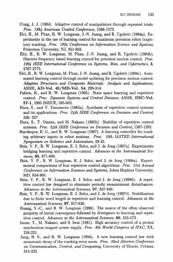
ILC DESIGNS 135
Craig, J. J. (1984). Adaptive control of manipulators through repeated trials. Proc. 1984 American Control Conference, 1566-1573.
Elci, H., M. Phan, R. W. Longman, J.-N. Juang, and R. Ugoletti (1994a). Experiments in the use of learning control for maximum precision robot trajectory tracking. Proc. 1994 Conference on Information Science and Systems, Princeton University, NJ, 951-958.
Elci, H., R. W. Longman, M. Phan, J.-N. Juang, and R. Ugoletti (1994b). Discrete frequency based learning control for precision motion control. Proc. 1994 IEEE International Conference on Systems, Man, and Cybernetics, 3, 2767-2773.
Elci, H., R. W. Longman, M. Phan, J.-N. Juang, and R. Ugoletti (1994c). Automated learning control through model updating for precision motion control. Adaptive Structures and Composite Materials: Analysis and Applications, ASME, AD-Vol. 45/MD-Vol. 54,299-314.
Fabien, B., and R. W. Longman (1995). State space learning and repetitive control. Proc. Dynamic Systems and Control Division, ASME, DSC-Vol. 57-1, 1995 IMECE, 595-602.
Hara, S., and Y. Yamamoto (1985a). Synthesis of repetitive control systems and its applications. Proc. 24th IEEE Conference on Decision and Control, 326- 327.
Hara, S., T. Omata, and M. Nakano (1985b). Stability of repetitive control systems. Proc. 24th IEEE Conference on Decision and Control, 1387-1392.
Harokopos, E. G., and R. W. Longman (1987). A learning controller for tracking arbitrary inputs in robot motions. Proc. 10th lASTED International Symposium on Robotics and Automation, 29-33.
Hsin, Y. P., R. W. Longman, E. J. Solcz, and J. de Jong (1997a). Experiments bridging learning and repetitive control. Advances in the Astronautical Sciences, 95, 671-690.
Hsin, Y. P., R. W. Longman, E. J. Solcz, and J. de Jong (1998a). Experimental comparisons of four repetitive control algorithms. Proc. 31st Annual Conference on Information Sciences and Systems, Johns Hopkins University, MD, 854-860.
Hsin, Y. P., R. W. Longman, E. J. Solcz, and J. de Jong (1998b). A repetitive control law designed to eliminate periodic measurement disturbances. Advances in the Astronautical Sciences, 97, 837-849.
Hsin, Y. P., R. W. Longman, E. J. Solcz, and J. de Jong (1997d). Stabilization due to finite word length in repetitive and learning control. Advances in the Astronautical Sciences, 97, 817-836.
Huang, Y.-C., and R. W. Longman (1996). The source of the often observed property of initial convergence followed by divergence in learning and repetitive control. Advances in the Astronautical Sciences, 90, 555-572.
Inoue, T., M. Nakano, and S. Iwai (1981). High accuracy control of a proton synchrotron magnet power supply. Proc. 8th World Congress of IFAC, XX, 216-221.
Jang, H. S., and R. W. Longman (1994). A new learning control law with monotonic decay of the tracking error norm. Proc. 32nd Allerton Conference on Communication, Control, and Computing, University of Illinois, Urbana, 314-323.
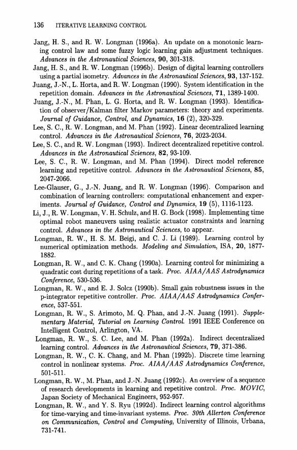
136 ITERATIVE LEARNING CONTROL
Jang, H. S., and R. W. Longman (1996a). An update on a monotonic learning control law and some fuzzy logic learning gain adjustment techniques. Advances in the Astronautical Sciences, 90, 301-318.
Jang, H. S., and R. W. Longman (1996b). Design of digital learning controllers using a partial isometry. Advances in the Astronautical Sciences, 93, 137-152.
Juang, J.-N., L. Horta, and R. W. Longman (1990). System identification in the repetition domain. Advances in the Astronautical Sciences, 71, 1389-1400.
Juang, J.-N., M. Phan, L. G. Horta, and R. W. Longman (1993). Identification of observer jKalman filter Markov parameters: theory and experiments. Journal of Guidance, Control, and Dynamics, 16 (2), 320-329.
Lee, S. C., R. W. Longman, and M. Phan (1992). Linear decentralized learning control. Advances in the Astronautical Sciences, 76, 2023-2034.
Lee, S. C., and R. W. Longman (1993). Indirect decentralized repetitive control. Advances in the Astronautical Sciences, 82, 93-109.
Lee, S. C., R. W. Longman, and M. Phan (1994). Direct model reference learning and repetitive control. Advances in the Astronautical Sciences, 85, 2047-2066.
Lee-Glauser, G., J.-N. Juang, and R. W. Longman (1996). Comparison and combination of learning controllers: computational enhancement and experiments. Journal of Guidance, Control and Dynamics, 19 (5), 1116-1123.
Li, J., R. W. Longman, V. H. Schulz, and H. G. Bock (1998). Implementing time optimal robot maneuvers using realistic actuator constraints and learning control. Advances in the Astronautical Sciences, to appear.
Longman, R. W., H. S. M. Beigi, and C. J. Li (1989). Learning control by numerical optimization methods. Modeling and Simulation, ISA, 20, 1877-1882.
Longman, R. W., and C. K. Chang (1990a). Learning control for minimizing a quadratic cost during repetitions of a task. Proc. AIAA/ AAS Astrodynamics Conference, 530-536.
Longman, R. W., and E. J. Solcz (1990b). Small gain robustness issues in the p-integrator repetitive controller. Proc. AIAA/ AAS Astrodynamics Conference, 537-551.
Longman, R. W., S. Arimoto, M. Q. Phan, and J.-N. Juang (1991). Supplementary Material, Tutorial on Learning Control. 1991 IEEE Conference on Intelligent Control, Arlington, VA.
Longman, R. W., S. C. Lee, and M. Phan (1992a). Indirect decentralized learning control. Advances in the Astronautical Sciences, 79, 371-386.
Longman, R. W., C. K. Chang, and M. Phan (1992b). Discrete time learning control in nonlinear systems. Proc. AIAA/ AAS Astrodynamics Conference, 501-511.
Longman, R. W., M. Phan, and J.-N. Juang (1992c). An overview of a sequence of research developments in learning and repetitive control. Proc. MOVIC, Japan Society of Mechanical Engineers, 952-957.
Longman, R. W., and Y. S. Ryu (1992d). Indirect learning control algorithms for time-varying and time-invariant systems. Proc. 30th Allerton Conference on Communication, Control and Computing, University of Illinois, Urbana, 731-741.
ILC DESIGNS 137
Longman, R. W., and Y.-C. Huang (1994). Use of unstable repetitive control for improved tracking accuracy. Adaptive Structures and Composite Materials: Analysis and Applications, ASME, AD-Vol. 45, 315-324.
Longman, R. W. (1995). Learning control, repetitive control, and vibration annihilation. Plenary Lecture, Proc. International Conference on Structural Dynamics, Vibration, Noise and Control, Hong Kong, 80-85.
Longman, R. W., and Y.-C. Huang (1996a). Analysis and frequency response of the alternating sign learning and repetitive control laws. Advances in the Astronautical Sciences, 90, 1105-1124.
Longman, R. W. (1996b). The range of possible iterative learning control laws to optimize robot tracking. ZAMM, 76 Sup. 3, 287-290.
Longman, R. W., and Y. Wang (1996c). Phase cancellation learning control using FFT weighted frequency response identification. Advances in the Astronautical Sciences, 93, 85-101.
Longman, R. W. (1996d). Learning and repetitive control design methodologies. Proceedings of the 9th Yale Workshop on Adaptive and Learning Systems, Yale University, CT, 124-129.
Longman, R. W., and C. P. Lo (1997a). Generalized holds, ripple attenuation, and tracking additional outputs in discrete time learning control. Journal of Guidance, Control and Dynamics, 20 (6), 1207-1214.
Longman, R. W. (1997b). Design methodologies in learning and repetitive control. Proceedings of the 2nd Asian Control Conference, Korea, 2, 39-42.
Longman, R. W., and Y. P. Hsin (1998a). On the need for stabilizing and the methods of stabilizing repetitive and learning controllers. Pro. 35th Allerton Conference on Communication, Control, and Computing, University of lllinois, Urbana, to appear.
Longman, R. W., and C. P. Lo (1998b). Frequency response based design of learning / repetitive controllers for nonlinear systems. Proc. Conference on Information Sciences and Systems, Princeton University, NJ, to appear.
Middleton, R. H., G. C. Goodwin, and R. W. Longman (1985). A method for improving the dynamic accuracy of a robot performing a repetitive task. University of Newcastle, Newcastle, Australia, Department of Electrical Engineering Technical Report EE8546. Also, International Journal of Robotics Research,8 (5), 1989,67-74.
Nakano, M., and S. Hara (1986). Microprocessor-based repetitive control. Microprocessor-Based Control Systems, 279-296.
Oh, S. J., R. W. Longman, and M. Q. Phan (1997). Use of de coupling basis functions in learning control for local learning and improved transients. Advances in the Astronautical Sciences, 95, 651-670.
Ornata, T., M. Nakano, and T. Inoue (1984). Applications of repetitive control method to multivariable systems. 11'ans. of SICE, 20 (9), 795-800.
Phan, M., and R. W. Longman (1988a). A mathematical theory of learning control for linear discrete multivariable systems. Proc. AIAA/ AAS Astrodynamics Conference, 740-746.
Phan, M., and R. W. Longman (1988b). Liapunov based model reference learning control. Proc. 26th Allerton Conference on Communication, Control and Computing, University of lllinois, Urbana, 927-936.

138 ITERATIVE LEARNING CONTROL
Phan, M., and R. W. Longman (1989a). Indirect learning control with guaranteed stability. Proceedings of the 1989 Conference on Information Sciences and Systems, Johns Hopkins University, MD, 125-131.
Phan, M., and R. W. Longman (1989b). Learning system identification. Modeling and Simulation, ISA, 20, 1857-1864.
Phan, M., Y. Wei, L. G. Horta, J.-N. Juang, and R. W. Longman (1989c). Learning control for slewing of a flexible panel. Proc. of the 7th VPI & SUjAIAA Symposium, L. Meirovitch, Editor, 39-52.
Phan, M., R. W. Longman, and J.-N. Juang (1989d). Indirect repetitive control for linear discrete multi variable systems. Proc. 27th Allerton Conference on Communication, Control, and Computing, University of Illinois, Urbana, 867-876.
Phan, M., J.-N. Juang, and R. W. Longman (1990). Recent developments in learning control and system identification for robots and structures. Dynamics of Flexible Structures in Space, C. L. Kirk, J. L. Junkins, Editors, Springer-Verlag, NY, 321-334.
Phan, M., L. G. Horta, J.-N. Juang, and R. W. Longman (1995). Improvement of observer/Kalman filter identification (OKID) by residual whitening. Journal of Vibrations and Acoustics, 117, 232-239.
Ryu, Y. S., R. W. Longman, E. J. Solcz, and J. de Jong (1994a). Experiments in the use of repetitive control in belt drive systems. Proc. 32nd Allerton Conference on Communication, Control, and Computing, University of Illinois, Urbana, 324-334.
Ryu, Y. S., and R. W. Longman (1994b). Use of anti-reset windup in integral control based learning control. Proc. IEEE International Conference on Systems, Man, and Cybernetics, 2617-2622.
Solcz, E. J., and R. W. Longman (1992a). Disturbance rejection in repetitive controllers. Advances in the Astronautical Sciences, 76, 2111-2130.
Solcz, E. J., and R. W. Longman (1992b). Robustness of repetitive controllers to frequency uncertainties. Proc. Conference on Information Sciences and Systems, Princeton University, NJ, 1009-1017.
Solcz, E. J., and R. W. Longman (1992c). Repetitive control in the presence of multiple periodic disturbances. Proc. AIAAj AAS Astrodynamics Conference, 486-500.
Tomizuka, M., T.-C. Tsao, K.-K. Chew (1989). Analysis and synthesis of discrete time repetitive controllers. Journal of Dynamic Systems, Measurement, and Control, 111 (3), 353-358.
Uchiyama, M. (1978). Formulation of high-speed motion pattern of a mechanical arm by trial. 1rans. Society for Instrumentation and Control Engineers, 14, 706-712.
Wang, Y., and R. W. Longman (1994). Limit cycle behavior and convergence to zero error in learning control with stick-slip friction. Proc. IEEE International Conference on Systems, Man, and Cybernetics, 3, 2775-2779.
Wang, Y., and R. W. Longman (1996a). Use of non-causal digital signal processing in learning and repetitive control. Advances in the Astronautical Sciences, 90, 649-668.

ILC DESIGNS 139
Wang, Y, and R. W. Longman (1996b). Monotonic vibration suppression using repetitive control and windowing techniques. Advances in the Astronautical Science, 93, 945-965.
Wen, H. P., and R. W. Longman (1997) . Conditions for convergence in indirect adaptive control based learning control. Advances in the Astronautical Sciences, 95, 623-642.
Wen, H. P., M. Q. Phan, and R. W. Longman (1998) . Bridging learning control and repetitive control using basis functions. Advances in the Astronautical Sciences, to appear.
Figure 7.1 Robotics Research robot used in learning control experiments
140 ITERATIVE LEARNING CONTROL
-initial -., . R.p..3 r\ .... R.p .• 1 - - ~p.'4
~ 5 J-_/ ... " ---~: g •. ,.. '" :~ ... . < .....
~ \' _.... ! ~ \ / i= -5 V
-II .!-----:~~2----=3-~4--=-5 -~'~-:!.7
Time (sec.)
Figure 7.2 Robot tracking errors, feedback only, and 6 repetitions using Control Law 1
Figure 7.3 Double reduction timing-belt drive system used in repetitive control experiments.
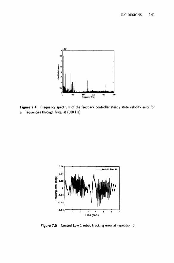
3.5
:m :m Frequency (Hz)
ILC DESIGNS 141
Figure 7.4 Frequency spectrum of the feedback controller steady state velocity error for all frequencies through Nyquist (500 Hz)
0.01 r-----.---,.-~-........ -...,.--~__,
0.04
i 0.02
I 0
2' :s -0.02
~ -0.04
-JoInI '1. Rap. 118
-0,0·D·'--~---~I--4-~---....I
Time (sec.)
Figure 7.5 Control Law 1 robot tracking error at repetition 6

142 ITERATIVE LEARNING CONTROL
2.S.-----~-~--~-...,
2
.~ 1.S (,!)
g 1 'E :ll O.S
....J
§ 0
los :::!;
20 40 60 80 100 Frequency (Hz)
Figure 7.6 Maximum learning gain vs. cutoff frequency, Control Law 1
".
0.5
·1
.1·~1L------::.(J':-.5 -~--::'::--7--1:":.5'----:!
Figure 7.7 Nyquist plot of the closed-loop timing-belt drive system
" ", o.a
0.6 '.
" 0.4
~ 0.2
N ~ a ~
I.(J·2
.(J.4 :
.(J.6
.(J.a
:lt5 ", ~.-.- .. .-
0.5 1.5 Real Axis
Figure 7.8 Nyquist plot for Control Law 2

REFERENCES 143
6.5
Figure 7.9 Control Law 2 timing-belt batch RMS errors vs. repetitions
fS ~ 5 w
~ a:: 4.5
3.50~-500=--:'1O=-OO-;;1500=--:2IXXI=---;:2500=-=3000=--'3500=' Repel~ion number
Figure 7.10 RMS error vs. repetitions for Control Law 3 using a 12th order instead of
18th order Butterworth filter
2)( 10"
1.8
1.6
1.4
~ 1.2
~ 1 c:: 0.8
..... 0=10-5 -0=10-6
Without Q
0.2
~~--~2IXXI~---4000==--~6000~---:BOOO==--~10000 Repetition Number
Figure 7.11 Stabilization by finite word length in integral control based learning

144 ITERATIVE LEARNING CONTROL
4 II: 10"
3.5
Figure 7.12 Control Law 3 velocity error spectrum at repetition 10.000
-JoInt1, Rep. 20
i 0,0
~ .,j, ............. ........ , ..... , .. 0
j -r' ~ ..."..r ....
I!! I- -0.0
-O,10~-t-"""2--a--4-~--.----J7·
11m. (88C.)
Figure 7.13 Tracking error at repetition 20. Control Law 6
10' r-----.-----........ --.------, -tI!!' :.:.:-..::;;1 ---MIl 4 ---Mill • - - _MIll .-- .... ,
.. ~---~---~---~ o ta
Figure 7.14 RMS error using Control Law 7 after 2 repetitions of inverse model learning
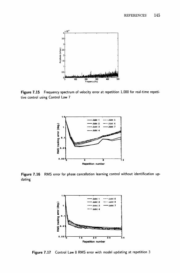
x 10" 4~--~-----.----~----~----.
35
Ii 2.5
i .g 2
'" ~15
Frequency (Hz)
REFERENCES 145
Figure 7.15 Frequency spectrum of velocity error at repetition 1,000 for real-time repetitive control using Control Law 7
10 -Joint! -----Joinl 5
~ -Joint 2 -·~·Joint 6
1 ----Joint 3 -Joint 7 :Eo g CD '" 0.1 c: :g I! ;;; 0.0 :::0 II:
0.00 0 4 8 1 2
Repetition number
Figure 7.16 RMS error for phase cancellation learning control without identification updating
10r-----~------~------~----_,
-Joint 1 -·-·-Joint 5
-Joint 2 - .... Joint e
---Joint 3 -Joint 7
-"-Joint 4
0.00~0~----~1~0~----~270----~3~0~--~40
Repetition number
Figure 7.17 Control Law 8 RMS error with model updating at repetition 3

146 ITERATIVE LEARNING CONTROL
o . o.
o.
! o. 1 c "j,
• 3
2
1
0
1
2 I~' .... .() .
.().3
.(J . 4
".I. .. ··nl r'
.(J:~ .1&1 .100 -50 0 &I 100 1&1 200 Leaming gain index
Figure 7.18 Truncated time domain learning gains for phase cancellation batch repetitive control of the timing-belt drive system
3.5
Figure 7.19 Frequency spectrum of the velocity error at repetition 50 for phase cancellation batch repetitive control of the belt drive system


![[Karger+ NIPS11] Iterative Learning for Reliable Crowdsourcing Systems](https://img.dokumen.tips/doc/110x75/5463d755b4af9f3f3f8b46cc/karger-nips11-iterative-learning-for-reliable-crowdsourcing-systems.jpg)


