Embed Size (px)
Citation preview

N° 29 – December 2012
Italian Journal of Pure andApplied Mathematics
ISSN 2239-0227
EDITOR-IN-CHIEFPiergiulio Corsini
Editorial BoardSaeid Abbasbandy
Reza AmeriLuisa Arlotti
Krassimir AtanassovMalvina Baica
Federico BartolozziRajabali Borzooei
Carlo CecchiniGui-Yun Chen
Domenico Nico ChillemiStephen Comer
Irina CristeaMohammad Reza Darafsheh
Bal Kishan DassBijan Davvaz
Alberto Felice De ToniFranco Eugeni
Giovanni FalconeYuming Feng
Antonino GiambrunoFurio Honsell
James JantosciakTomas Kepka
David KinderlehrerAndrzej Lasota
Violeta LeoreanuMario Marchi
Donatella MariniAngelo MarzolloAntonio Maturo
M. Reza MoghadamPetr Nemec
Vasile OproiuLivio C. PiccininiGoffredo PieroniFlavio Pressacco
Vito RobertoIvo Rosenberg
Paolo SalmonMaria Scafati Tallini
Kar Ping ShumAlessandro SilvaSergio Spagnolo
Hari M. SrivastavaMarzio Strassoldo
Yves SureauCarlo TassoIoan TofanAldo Ventre
Thomas VougiouklisHans Weber
Yunqiang YinMohammad Mehdi Zahedi
Fabio ZanolinPaolo Zellini
Jianming Zhan
F O R U M

EDITOR-IN-CHIEF
Piergiulio Corsini Department of Civil Engineering and Architecture Via delle Scienze 206 - 33100 Udine, Italy [email protected]
VICE-CHIEF
Violeta Leoreanu
MANAGING BOARD
Domenico Chillemi, CHIEFPiergiulio CorsiniIrina CristeaFurio HonsellVioleta LeoreanuElena MocanuLivio PiccininiFlavio PressaccoNorma Zamparo
EDITORIAL BOARD
Saeid Abbasbandy Dept. of Mathematics, Imam Khomeini International University, Ghazvin, 34149-16818, Iran [email protected]
Reza Ameri Department of Mathematics University of Tehran Tehran, Iran [email protected]
Luisa Arlotti Department of Civil Engineering and Architecture Via delle Scienze 206 - 33100 Udine, Italy [email protected]
Krassimir Atanassov Centre of Biomedical Engineering, Bulgarian Academy of Science BL 105 Acad. G. Bontchev Str. 1113 Sofia, Bulgaria [email protected]
Malvina Baica University of Wisconsin-Whitewater Dept. of Mathematical and Computer Sciences Whitewater, W.I. 53190, U.S.A. [email protected]
Federico Bartolozzi Dipartimento di Matematica e Applicazioni via Archirafi 34 - 90123 Palermo, Italy [email protected]
Rajabali Borzooei Department of Mathematics Shahid Beheshti University Tehran, Iran [email protected]
Carlo Cecchini Dipartimento di Matematica e Informatica Via delle Scienze 206 - 33100 Udine, Italy [email protected]
Gui-Yun Chen School of Mathematics and Statistics, Southwest University, 400715, Chongqing, China [email protected]
Domenico (Nico) Chillemi Executive IT Specialist, IBM Software Group IBM Italy SpA Via Sciangai 53 – 00144 Roma, Italy [email protected]
Stephen Comer Department of Mathematics and Computer Science The Citadel, Charleston S. C. 29409, USA [email protected]
Irina Cristea Department of Civil Engineering and Architecture Via delle Scienze 206 - 33100 Udine, Italy [email protected]
Mohammad Reza Darafsheh School of Mathematics, College of Science University of Tehran Tehran – Iran [email protected]
Bal Kishan Dass Department of Mathematics University of Delhi, Delhi - 110007, India [email protected]
Bijan Davvaz Department of Mathematics, Yazd University, Yazd, Iran [email protected]
Alberto Felice De Toni Faculty of Engineering Udine University Via delle Scienze 206 - 33100 Udine, Italy [email protected]
Franco Eugeni Dipartimento di Metodi Quantitativi per l'Economia del Territorio Università di Teramo, Italy [email protected]
Giovanni Falcone Dipartimento di Metodi e Modelli Matematici viale delle Scienze Ed. 8 90128 Palermo, Italy [email protected]
Yuming Feng College of Math. and Comp. Science, Chongqing Three-Gorges University, Wanzhou, Chongqing, 404000, P.R.China [email protected]
Antonino Giambruno Dipartimento di Matematica e Applicazioni via Archirafi 34 - 90123 Palermo, Italy [email protected]
Furio Honsell Dipartimento di Matematica e Informatica Via delle Scienze 206 - 33100 Udine, Italy [email protected]
James Jantosciak Department of Mathematics Brooklyn College (CUNY) Brooklyn, New York 11210, USA [email protected]
Tomas Kepka MFF-UK Sokolovská 83 18600 Praha 8,Czech Republic [email protected]
David Kinderlehrer Department of Mathematical Sciences Carnegie Mellon University Pittsburgh, PA15213-3890, USA [email protected]
Andrzej Lasota Silesian University Institute of Mathematics Bankova 14 40-007 Katowice, Poland [email protected]
Violeta Leoreanu Faculty of Mathematics Al. I. Cuza University 6600 Iasi, Romania [email protected]
Mario Marchi Università Cattolica del Sacro Cuore via Trieste 17, 25121 Brescia, Italy [email protected]
Donatella Marini Dipartimento di Matematica Via Ferrata 1- 27100 Pavia, Italy [email protected]
Angelo Marzollo Dipartimento di Matematica e Informatica Via delle Scienze 206 - 33100 Udine, Italy [email protected]
Antonio Maturo University of Chieti-Pescara, Department of Social Sciences, Via dei Vestini, 31 66013 Chieti, Italy [email protected]
M. Reza Moghadam Faculty of Mathematical Science Ferdowsi University of Mashhadh P.O.Box 1159 - 91775 Mashhad, Iran [email protected] Petr Nemec Czech University of Life Sciences, Kamycka’ 129 16521 Praha 6, Czech Republic [email protected]
Vasile Oproiu Faculty of Mathematics Al. I. Cuza University 6600 Iasi, Romania [email protected]
Livio C. Piccinini Department of Civil Engineering and Architecture Via delle Scienze 206 - 33100 Udine, Italy [email protected]
Goffredo Pieroni Dipartimento di Matematica e Informatica Via delle Scienze 206 - 33100 Udine, Italy [email protected]
Flavio Pressacco Dept. of Economy and Statistics Via Tomadini 30 33100, Udine, Italy [email protected]
Vito Roberto Dipartimento di Matematica e Informatica Via delle Scienze 206 - 33100 Udine, Italy [email protected]
Ivo Rosenberg Departement de Mathematique et de Statistique Université de Montreal C.P. 6128 Succursale Centre-Ville Montreal, Quebec H3C 3J7 - Canada [email protected]
Paolo Salmon Dipartimento di Matematica Università di Bologna Piazza di Porta S. Donato 5 40126 Bologna, Italy [email protected]
Maria Scafati Tallini Dipartimento di Matematica "Guido Castelnuovo" Università La Sapienza Piazzale Aldo Moro 2 - 00185 Roma, Italy [email protected]
Kar Ping Shum Faculty of Science The Chinese University of Hong Kong Hong Kong, China (SAR) [email protected]
Alessandro Silva Dipartimento di Matematica "Guido Castelnuovo" Università La Sapienza Piazzale Aldo Moro 2 - 00185 Roma, Italy [email protected]
Sergio Spagnolo Scuola Normale Superiore Piazza dei Cavalieri 7 - 56100 Pisa, Italy [email protected]
Hari M. Srivastava Department of Mathematics and Statistics University of Victoria Victoria, British Columbia V8W3P4, Canada [email protected]
Marzio Strassoldo Department of Statistical Sciences Via delle Scienze 206 - 33100 Udine, Italy [email protected]
Yves Sureau 27, rue d'Aubiere 63170 Perignat, Les Sarlieve - France [email protected]
Carlo Tasso Dipartimento di Matematica e Informatica Via delle Scienze 206 - 33100 Udine, Italy [email protected]
Ioan Tofan Faculty of Mathematics Al. I. Cuza University 6600 Iasi, Romania [email protected]
Aldo Ventre Seconda Università di Napoli, Fac. Architettura, Dip. Cultura del Progetto Via San Lorenzo s/n 81031 Aversa (NA), Italy [email protected]
Thomas Vougiouklis Democritus University of Thrace, School of Education, 681 00 Alexandroupolis. Greece [email protected]
Hans Weber Dipartimento di Matematica e Informatica Via delle Scienze 206 - 33100 Udine, Italy [email protected]
Yunqiang Yin School of Mathematics and Information Sciences, East China Institute of Technology, Fuzhou, Jiangxi 344000, P.R. China [email protected]
Mohammad Mehdi Zahedi Department of Mathematics, Faculty of Science Shahid Bahonar, University of Kerman Kerman, Iran [email protected]
Fabio Zanolin Dipartimento di Matematica e Informatica Via delle Scienze 206 - 33100 Udine, Italy [email protected]
Paolo Zellini Dipartimento di Matematica Università degli Studi Tor Vergata, via Orazio Raimondo (loc. La Romanina) - 00173 Roma, Italy [email protected]
Jianming Zhan Department of Mathematics, Hubei Institute for Nationalities Enshi, Hubei Province,445000, China [email protected]
ITALIAN JOURNAL OF PURE AND APPLIED MATHEMATICS – N. 29-2012
Italian Journal of Pure and Applied MathematicsISSN 2239-0227
Web Sitehttp://ijpam.uniud.it/journal/home.html
EDITOR-IN-CHIEFPiergiulio Corsini
Department of Civil Engineering and ArchitectureVia delle Scienze 206 - 33100 Udine, Italy
Vice-CHIEF Violeta Leoreanu
Managing BoardDomenico Chillemi, CHIEF
Piergiulio CorsiniIrina Cristea
Furio HonsellVioleta Leoreanu
Elena MocanuLivio Piccinini
Flavio PressaccoNorma Zamparo
Editorial Board
Saeid AbbasbandyReza AmeriLuisa Arlotti
Krassimir AtanassovMalvina Baica
Federico BartolozziRajabali Borzooei
Carlo CecchiniGui-Yun Chen
Domenico Nico ChillemiStephen Comer
Irina CristeaMohammad Reza Darafsheh
Bal Kishan DassBijan Davvaz
Alberto Felice De ToniFranco Eugeni
Giovanni FalconeYuming Feng
Antonino GiambrunoFurio Honsell
James JantosciakTomas Kepka
David KinderlehrerAndrzej Lasota
Violeta LeoreanuMario Marchi
Donatella MariniAngelo MarzolloAntonio Maturo
M. Reza MoghadamPetr Nemec
Vasile OproiuLivio C. PiccininiGoffredo PieroniFlavio Pressacco
Vito RobertoIvo Rosenberg
Paolo SalmonMaria Scafati Tallini
Kar Ping ShumAlessandro SilvaSergio Spagnolo
Hari M. SrivastavaMarzio Strassoldo
Yves SureauCarlo TassoIoan Tofan
Aldo VentreThomas Vougiouklis
Hans WeberYunqiang Yin
Mohammad Mehdi ZahediFabio ZanolinPaolo Zellini
Jianming Zhan
Forum Editrice Universitaria Udinese SrlVia Palladio 8 - 33100 Udine
Tel: +39-0432-26001, Fax: [email protected]
1
ITALIAN JOURNAL OF PURE AND APPLIED MATHEMATICS – N. 29-2012
Italian Journal of Pure and Applied Mathematics – N. 29–2012
A new predictor-corrector algorithm for SDP with polynomial convergenceFeixiang Chen, Yuming Feng pp. 7-24Pseudo-D-lattices and topologies generated by measuresAnna Avallone, Paolo Vitolo pp. 25-42On injectivity of projection and separated projection algebrasM.M. Ebrahimi, M. Mahmoudi pp. 43-54Quasi-permutation representations of some minimal non-abelian q-groupsMohammad Hassan Abbaspour, Houshang Behravesh pp. 55-62An analytical solution of fluid flow through narrowing systemsA.D. Patel, I.A. Salehbhai, J. Banerjee, V.K. Katiyar, A.K. Shukla pp. 63-70On generalized Hilbert algebrasR.A. Borzooei, J. Shohani pp. 71-86mth Power symmetric n-sigraphsR. Rangarajan, P. Siva Kota Reddy, N.D. Soner pp. 87-92Common fixed point theorems for finite number of mappings without continuity and compatibility on uniformly convex Banach spaceSushil Sharma, Alok Pande, Chetna Kothari pp. 93-108Error locating codes dealing with repeated burst errorsBal Kishan Dass, Ritu Arora pp. 109-118M-injectivity in the category Act-S Leila Shahbaz pp. 119-134On Köthe-Toeplitz duals of some new and generalized difference sequence spacesA.A. Ansari, V.K. Chaudhry pp. 135-148Fuzzy hypervector spaces (redefined) R. Ameri, M. Motameni pp. 149-162Sur les algèbres de Lie d'un système de champs de vecteurs permutablesH.S.G. Ravelonirina, P. Randriambololondrantomalala, M. Anona pp. 163-174C-essentialness and well-behavedness of C-injectivity in Act-SLeila Shahbaz pp. 175-186Numbers in the n dimensional spaceNicola D'Alfonso pp. 187-300A radical property of hyperringsA. Ashokumar, M. Velrajan pp. 301-308Multi-objective decision making based on fuzzy events and their coherent (fuzzy) measuresAntonio Maturo pp. 309-324The category of hyper S-actsLeila Shahbaz pp. 325-332Maximal partial line spreads of PG(3; q), q evenMaria Scafati Tallini pp. 333-340Hv-Structures and the bar in questionnaires Pipina Nikolaidou, Thomas Vougiouklis pp. 341-350Related fixed point theorem for six mappings on~three~modified intuitionistic fuzzy metric spacesSushil Sharma, Prashant Tilwankar pp. 351-364Geometric equivalence between the Veblen and Desargues theorems and between the Pappus-Pascal and the "Three stars theorems"Maria Scafati Tallini pp. 365-370Three representations of a hyperbolic quadric of PG(3; q) in AG(2; q)Maria Scafati Tallini pp. 371-386Recognition of A10 and L4(4) by two special conjugacy class sizesYanheng Chen, Guiyun Chen pp. 387-394The groups of two classes of certain cyclically presented groups are essentially 3-generatedDevon Roy Stoddart pp. 395-402n-fold positive implicative hyper K-idealsP. Babari, M. Pirasghari, M.M. Zahedi pp. 403-418
ISSN 2239-0227
2

ITALIAN JOURNAL OF PURE AND APPLIED MATHEMATICS – N. 29-2012
Exchanges
Up to July 2011 this journal is exchanged with the following periodicals:
1. Acta Cybernetica - Szeged H2. Acta Mathematica et Informatica Universitatis Ostraviensis CZ3. Acta Mathematica Vietnamica – Hanoi VN4. Acta Mathematica Sinica, New Series – Beijing RC5. Acta Scientiarum Mathematicarum – Szeged H6. Acta Universitatis Lodziensis – Lodz PL7. Acta Universitatis Palackianae Olomucensis, Mathematica – Olomouc CZ8. Actas del tercer Congreso Dr. Antonio A.R. Monteiro - Universidad Nacional del Sur Bahía Blanca AR9. Algebra Colloquium - Chinese Academy of Sciences, Beijing PRC10. Alxebra - Santiago de Compostela E11. Analele Ştiinţifice ale Universităţii “Al. I Cuza” - Iaşi RO12. Analele Universităţii din Timişoara - Universitatea din Timişoara RO13. Annales Academiae Scientiarum Fennicae Mathematica - Helsinki SW14. Annales de la Fondation Louis de Broglie - Paris F15. Annales Mathematicae Silesianae – Katowice PL16. Annales Scientif. Université Blaise Pascal - Clermont II F17. Annales sect. A/Mathematica – Lublin PL18. Annali dell’Università di Ferrara, Sez. Matematica I19. Annals of Mathematics - Princeton - New Jersey USA20. Applied Mathematics and Computer Science -Technical University of Zielona Góra PL21. Archivium Mathematicum - Brno CZ22. Atti del Seminario di Matematica e Fisica dell’Università di Modena I23. Atti dell’Accademia delle Scienze di Ferrara I24. Automatika i Telemekhanika - Moscow RU25. Boletim de la Sociedade Paranaense de Matematica - San Paulo BR26. Bolétin de la Sociedad Matemática Mexicana - Mexico City MEX27. Bollettino di Storia delle Scienze Matematiche - Firenze I28. Buletinul Academiei de Stiinte - Seria Matem. - Kishinev, Moldova CSI29. Buletinul Ştiinţific al Universităţii din Baia Mare - Baia Mare RO30. Buletinul Ştiinţific şi Tecnic-Univ. Math. et Phyis. Series Techn. Univ. - Timişoara RO31. Buletinul Universităţii din Braşov, Seria C - Braşov RO32. Bulletin de la Classe de Sciences - Acad. Royale de Belgique B33. Bulletin de la Societé des Mathematiciens et des Informaticiens de Macedoine MK34. Bulletin de la Société des Sciences et des Lettres de Lodz - Lodz PL35. Bulletin de la Societé Royale des Sciences - Liege B36. Bulletin Mathematics and Physics - Assiut ET37. Bulletin Mathématique - Skopje Macedonia MK38. Bulletin Mathématique de la S.S.M.R. - Bucharest RO39. Bulletin of the Australian Mathematical Society - St. Lucia - Queensland AUS40. Bulletin of the Faculty of Science - Assiut University ET41. Bulletin of the Faculty of Science - Mito, Ibaraki J42. Bulletin of the Greek Mathematical Society - Athens GR43. Bulletin of the Iranian Mathematical Society - Tehran IR44. Bulletin of the Korean Mathematical Society - Seoul ROK45. Bulletin of the Malaysian Mathematical Sciences Society - Pulau Pinang MAL46. Bulletin of the Transilvania University of Braşov - Braşov RO47. Bulletin of the USSR Academy of Sciences - San Pietroburgo RU48. Bulletin for Applied Mathematics - Technical University Budapest H49. Busefal - Université P. Sabatier - Toulouse F50. Calculus CNR - Pisa I51. Chinese Annals of Mathematics - Fudan University – Shanghai PRC52. Chinese Quarterly Journal of Mathematics - Henan University PRC53. Classification of Commutative FPF Ring - Universidad de Murcia E54. Collectanea Mathematica - Barcelona E55. Collegium Logicum - Institut für Computersprachen Technische Universität Wien A56. Colloquium - Cape Town SA57. Colloquium Mathematicum - Instytut Matematyczny - Warszawa PL58. Commentationes Mathematicae Universitatis Carolinae - Praha CZ59. Computer Science Journal of Moldova CSI60. Contributi - Università di Pescara I61. Cuadernos - Universidad Nacional de Rosario AR62. Czechoslovak Mathematical Journal - Praha CZ63. Demonstratio Mathematica - Warsawa PL64. Discussiones Mathematicae - Zielona Gora PL
3
ITALIAN JOURNAL OF PURE AND APPLIED MATHEMATICS – N. 29-2012
65. Divulgaciones Matemáticas - Universidad del Zulia YV66. Doctoral Thesis - Department of Mathematics Umea University SW67. Extracta Mathematicae - Badajoz E68. Fasciculi Mathematici - Poznan PL69. Filomat - University of Nis SRB70. Forum Mathematicum - Mathematisches Institut der Universität Erlangen D71. Functiones et Approximatio Commentarii Mathematici - Adam Mickiewicz University L72. Funkcialaj Ekvaciaj - Kobe University J73. Fuzzy Systems & A.I. Reports and Letters - Iaşi University RO74. General Mathematics - Sibiu RO75. Geometria - Fasciculi Mathematici - Poznan PL76. Glasnik Matematicki - Zagreb CRO77. Grazer Mathematische Berichte – Graz A78. Hiroshima Mathematical Journal - Hiroshima J79. Hokkaido Mathematical Journal - Sapporo J80. Houston Journal of Mathematics - Houston - Texas USA81. Illinois Journal of Mathematics - University of Illinois Library - Urbana USA82. Informatica - The Slovene Society Informatika - Ljubljana SLO83. Internal Reports - University of Natal - Durban SA84. International Journal of Computational and Applied Mathematics – University of Qiongzhou, Hainan PRC85. International Journal of Science of Kashan University - University of Kashan IR86. Iranian Journal of Science and Technology - Shiraz University IR87. Irish Mathematical Society Bulletin - Department of Mathematics - Dublin IRL88. IRMAR - Inst. of Math. de Rennes - Rennes F89. Israel Mathematical Conference Proceedings - Bar-Ilan University - Ramat -Gan IL90. Izvestiya: Mathematics - Russian Academy of Sciences and London Mathematical Society RU91. Journal of Applied Mathematics and Computing – Dankook University, Cheonan – Chungnam ROK92. Journal of Basic Science - University of Mazandaran – Babolsar IR93. Journal of Beijing Normal University (Natural Science) - Beijing PRC94. Journal of Dynamical Systems and Geometric Theory - New Delhi IND95. Journal Egyptian Mathematical Society – Cairo ET96. Journal of Mathematical Analysis and Applications - San Diego California USA97. Journal of Mathematics of Kyoto University - Kyoto J98. Journal of Science - Ferdowsi University of Mashhad IR99. Journal of the Bihar Mathematical Society - Bhangalpur IND100. Journal of the Faculty of Science – Tokyo J101. Journal of the Korean Mathematical Society - Seoul ROK102. Journal of the Ramanujan Mathematical Society - Mysore University IND103. Journal of the RMS - Madras IND104. Kumamoto Journal of Mathematics - Kumamoto J105. Kyungpook Mathematical Journal - Taegu ROK106. L’Enseignement Mathématique - Genève CH107. La Gazette des Sciences Mathématiques du Québec - Université de Montréal CAN108. Le Matematiche - Università di Catania I109. Lecturas Matematicas, Soc. Colombiana de Matematica - Bogotà C110. Lectures and Proceedings International Centre for Theorical Phisics - Trieste I111. Lucrările Seminarului Matematic – Iaşi RO112. m-M Calculus - Matematicki Institut Beograd SRB113. Matematicna Knjiznica - Ljubljana SLO114. Mathematica Balcanica – Sofia BG115. Mathematica Bohemica - Academy of Sciences of the Czech Republic Praha CZ116. Mathematica Macedonica, St. Cyril and Methodius University, Faculty of Natural Sciences and Mathematics - Skopje MK117. Mathematica Montisnigri - University of Montenegro - Podgorica MNE118. Mathematica Moravica - Cacak SRB119. Mathematica Pannonica - Miskolc - Egyetemvaros H120. Mathematica Scandinavica - Aarhus - Copenhagen DK121. Mathematica Slovaca - Bratislava CS122. Mathematicae Notae - Universidad Nacional de Rosario AR123. Mathematical Chronicle - Auckland NZ124. Mathematical Journal - Academy of Sciences - Uzbekistan CSI125. Mathematical Journal of Okayama University - Okayama J126. Mathematical Preprint - Dep. of Math., Computer Science, Physics – University of Amsterdam NL127. Mathematical Reports - Kyushu University - Fukuoka J128. Mathematics Applied in Science and Technology – Sangyo University, Kyoto J129. Mathematics Reports Toyama University - Gofuku J130. MAT - Prepublicacions - Universidad Austral AR131. Mediterranean Journal of Mathematics – Università di Bari I132. Memoirs of the Faculty of Science - Kochi University - Kochi J133. Memorias de Mathematica da UFRJ - Istituto de Matematica - Rio de Janeiro BR134. Memorie linceee - Matematica e applicazioni - Accademia Nazionale dei Lincei I135. Mitteilungen der Naturforschenden Gesellschaften beider Basel CH136. Monografii Matematice - Universitatea din Timişoara RO137. Monthly Bulletin of the Mathematical Sciences Library – Abuja WAN
4

ITALIAN JOURNAL OF PURE AND APPLIED MATHEMATICS – N. 29-2012
138. Nagoya Mathematical Journal - Nagoya University,Tokyo J139. Neujahrsblatt der Naturforschenden Gesellschaft - Zürich CH140. New Zealand Journal of Mathematics - University of Auckland NZ141. Niew Archief voor Wiskunde - Stichting Mathematicae Centrum – Amsterdam NL142. Nihonkai Mathematical Journal - Niigata J143. Notas de Algebra y Analisis - Bahia Blanca AR144. Notas de Logica Matematica - Bahia Blanca AR145. Notas de Matematica Discreta - Bahia Blanca AR146. Notas de Matematica - Universidad de los Andes, Merida YV147. Notas de Matematicas - Murcia E148. Note di Matematica - Lecce I149. Novi Sad Journal of Mathematics - University of Novi Sad SRB150. Obzonik za Matematiko in Fiziko - Ljubljana SLO151. Octogon Mathematical Magazine - Braşov RO152. Osaka Journal of Mathematics - Osaka J153. Periodica Matematica Hungarica - Budapest H154. Periodico di Matematiche - Roma I155. Pliska - Sofia BG156. Portugaliae Mathematica - Lisboa P157. Posebna Izdanja Matematickog Instituta Beograd SRB158. Pre-Publicaçoes de Matematica - Univ. de Lisboa P159. Preprint - Department of Mathematics - University of Auckland NZ160. Preprint - Institute of Mathematics, University of Lodz PL161. Proceeding of the Indian Academy of Sciences - Bangalore IND162. Proceeding of the School of Science of Tokai University - Tokai University J163. Proceedings - Institut Teknology Bandung - Bandung RI164. Proceedings of the Academy of Sciences Tasked – Uzbekistan CSI165. Proceedings of the Mathematical and Physical Society of Egypt – University of Cairo ET166. Publicaciones del Seminario Matematico Garcia de Galdeano - Zaragoza E167. Publicaciones - Departamento de Matemática Universidad de Los Andes Merida YV168. Publicaciones Matematicas del Uruguay - Montevideo U169. Publicaciones Mathematicae - Debrecen H170. Publicacions mathematiques - Universitat Autonoma, Barcelona E171. Publications de l’Institut Mathematique - Beograd SRB172. Publications des Séminaires de Mathématiques et Informatiques de Rennes F173. Publications du Departmenet de Mathematiques, Université Claude Bernard - Lyon F174. Publications Mathematiques - Besançon F175. Publications of Serbian Scientific Society - Beograd SRB176. Publikacije Elektrotehnickog Fakulteta - Beograd SRB177. Pure Mathematics and Applications - Budapest H178. Quaderni di matematica - Dip. to di Matematica – Caserta I179. Qualitative Theory of Dynamical Systems - Universitat de Lleida E180. Quasigroups and Related Systems - Academy of Science - Kishinev Moldova CSI181. Ratio Mathematica - Università di Pescara I182. Recherche de Mathematique - Institut de Mathématique Pure et Appliquée Louvain-la-Neuve B183. Rendiconti del Seminario Matematico dell’Università e del Politecnico – Torino I184. Rendiconti del Seminario Matematico - Università di Padova I185. Rendiconti dell’Istituto Matematico - Università di Trieste I186. Rendiconti di Matematica e delle sue Applicazioni - Roma I187. Rendiconti lincei - Matematica e applicazioni - Accademia Nazionale dei Lincei I188. Rendiconti Sem. - Università di Cagliari I189. Report series - Auckland NZ190. Reports Math. University of Stockholm - Stockholm SW191. Reports - University Amsterdam NL192. Reports of Science Academy of Tajikistan – Dushanbe TAJ193. Research Reports - Cape Town SA194. Research Reports - University of Umea - Umea SW195. Research Report Collection (RGMIA) Melbourne AUS196. Resenhas do Instituto de Matemática e Estatística da universidadae de São Paulo BR197. Review of Research, Faculty of Science, Mathematics Series - Institute of Mathematics University of Novi Sad SRB198. Review of Research Math. Series - Novi Sad YN199. Revista Ciencias Matem. - Universidad de la Habana C200. Revista Colombiana de Matematicas - Bogotà C201. Revista de Matematicas Aplicadas - Santiago CH202. Revue Roumaine de Mathematiques Pures et Appliquées - Bucureşti RO203. Ricerca Operativa AIRO - Genova I204. Ricerche di Matematica - Napoli I205. Rivista di Matematica - Università di Parma I206. Sains Malaysiana - Selangor MAL207. Saitama Mathematical Journal - Saitama University J208. Sankhya - Calcutta IND209. Sarajevo Journal of Mathematics BIH210. Sciences Bulletin, DPRK, Pyongyang KR
5
ITALIAN JOURNAL OF PURE AND APPLIED MATHEMATICS – N. 29-2012
211. Scientific Rewiev - Beograd SRB212. Semesterbericht Funktionalanalysis - Tübingen D213. Séminaire de Mathematique - Université Catholique, Louvain la Neuve B214. Seminario di Analisi Matematica - Università di Bologna I215. Serdica Bulgaricae Publicaciones Mathematicae - Sofia BG216. Serdica Mathematical Journal - Bulgarian Academy of Sciences, University of Sofia BG217. Sitzungsberichte der Mathematisch Naturwissenschaflichen Klasse Abteilung II – Wien A218. Southeast Asian Bulletin of Mathematics - Southeast Asian Mathematical Society PRC219. Studia Scientiarum Mathematica Hungarica – Budapest H220. Studia Universitatis Babes Bolyai - Cluj Napoca RO221. Studii şi Cercetări Matematice - Bucureşti RO222. Studii şi Cercetări Ştiinţifice, ser. Matematică - Universitatea din Bacău RO223. Sui Hak - Pyongyang DPR of Korea KR224. Tamkang Journal of Mathematics - Tamsui - Taipei TW225. Thai Journal of Mathematics – Chiang Mai TH226. The Journal of the Academy of Mathematics Indore IND227. The Journal of the Indian Academy of Mathematics - Indore IND228. The Journal of the Nigerian Mathematical Society (JNMS) - Abuja WAN229. Theoretical and Applied Mathematics – Kongju National University ROK230. Thesis Reprints - Cape Town SA231. Tohoku Mathematical Journal – Sendai J232. Trabalhos do Departamento de Matematica Univ. - San Paulo BR233. Travaux de Mathematiques – Bruxelles B234. Tsukuba Journal of Mathematics - University of Tsukuba J235. UCNW Math. Preprints Prifysgol Cymru - University of Wales – Bangor GB236. Ukranii Matematiskii Journal – Kiev RU237. Uniwersitatis Iagiellonicae Acta Mathematica – Krakow PL238. Verhandlungen der Naturforschenden Gesellschaft – Basel CH239. Vierteljahrsschrift der Naturforschenden Gesellschaft – Zürich CH240. Volumenes de Homenaje - Universidad Nacional del Sur Bahía Blanca AR241. Yokohama Mathematical Journal – Yokohama J242. Yugoslav Journal of Operations Research – Beograd SRB243. Zbornik Radova Filozofskog – Nis SRB244. Zbornik Radova – Kragujevac SRB245. Zeitschrift für Mathematick Logic und Grundlagen der Math. – Berlin D246. IJMSI - Iranian Journal of Mathematical Sciences & Informatics, Tarbiat Modares University, Tehran IR247. Scientific Studies and Research, Vasile Alecsandri University Bacau RO248. Bulletin of Society of Mathematiciens Banja Luka, Banja Luka BiH
6

italian journal of pure and applied mathematics – n. 29−2012 (7−14) 7
A NEW PREDICTOR-CORRECTOR ALGORITHM FOR SDPWITH POLYNOMIAL CONVERGENCE1
Feixiang Chen
Yuming Feng
School of Mathematics and StatisticsChongqing Three Gorges UniversityWanzhou, Chongqing, 404000P.R. Chinae-mail: [email protected]
Abstract. We establish the polynomiality of primal-dual interior-point algorithms forSDP based on the direction of the M-Z family of search directions. We show thatthe polynomial iteration-complexity bounds of the well known algorithms for linearprogramming, namely, the predictor-corrector algorithm, carry over to the context ofSDP.
Keywords: interior-point algorithm; polynomial complexity; path-following methods;semidefinite programming problems.
1. Introduction
Several authors have discussed generalizations of interior-point algorithms for li-near programming (LP) to the context of semidefinite programming (SDP). Thelandmark work in this direction is due to Nesterov and Nemirovskii [1], where ageneral approach for using interior-point algorithms for solving convex programsis proposed, based on the notion of self-concordant functions. They show thatthe problem of minimizing a linear function over a convex set can be solved in’polynomial time’ as long as a self-concordant barrier function for the convexset is known. On the other hand, Alizadeh [2] extends Ye’s projective potentialreduction algorithm for LP to SDP and argues that many known interior pointalgorithms for LP can also be transformed into algorithms for SDP in a mechanicalway. Since then many authors have proposed interior-point algorithms for solvingthe SDP, including Alizadeh, Haeberly and Overton [3], Kojima, Shida [4]andShindoh, Kojima, and Hara [5], Monteiro [6], [7], Monteiro and Zhang [8], [9],and Zhang [10]. Most of these more recent works are concentrated on primal-dualalgorithms.
1Research is supported by Natural Science Foundation of Chongqing Municipal EducationCommission (No.KJ091104).
8 feixiang chen, yuming feng
Notation and terminology
The set of all symmetric n × n matrices is denoted by Sn. For Q ∈ Sn, Q º 0means Q is positive semidefinite and Q Â 0 means Q is positive definite, respec-
tively. The trace of a matrix Q ∈ Rn×n is denoted by Tr Q ≡n∑
i=1
Qii. The inner
product between P and Q in Rm×n is defined as P • Q ≡ Tr P T Q. The Eu-clidean norm and its associated operator norm are both denoted by ‖ ‖; hence,‖Q‖ ≡ max‖u‖=1 ‖Qu‖ for any Q ∈ Rn×n. The Frobenius norm of Q ∈ Rn×n is‖Q‖F ≡ (Q •Q)1/2. We frequently use the inequalities Sn
+ and Sn++ denote the set
of all matrices in Sn which are positive semidefinite and positive definite, respec-tively. It is known that for each V ∈ Sn
+, there exists a unique U ∈ Sn+, such that
U2 = V. The matrix U is called the square root of V and is denoted by V 1/2.
2. The SDP problem and preliminary discussion
In this section, we describe the SDP in symmetric matrices considered in thispaper, state our assumptions, and derive the Newton direction for the centralpath equation. We also give some existence results for this Newton direction andstate a generic path-following algorithm based on it.
Given C ∈ Sn and (Ai, bi) ∈ Sn × R for i = 1, ..., m, a primal-dual pair ofSDP problems is defined as
(P ) minC •X : Ai •X = bi, i = 1, ..., m, X º 0,(2.1)
(D) max
bT y :
m∑i=1
yiAi + S = C, S º 0
,(2.2)
where b ≡ (b1, ..., bm)T .
The set of interior feasible solutions of (1) and (2) are
F 0(P ) ≡ X ∈ S : X : Ai •X = bi, i = 1, ..., m, X Â 0F 0(D) ≡ (S, y) ∈ S ×Rm :
∑mi=1 yiAi + S = C, S Â 0
respectively. Throughout this paper, we assume that F 0(P ) × F 0(D) 6= φ andthat the matrices Ai, i = 1, . . . , m, are linearly independent. Under the firstassumption, it is well known that both (1) and (2) have optimal solutions X∗ and(S∗, y∗) such that C •X∗ = bT y∗, i.e., the optimal values of (1) and (2) coincide.The last condition, called the strong duality, can be alternatively expressed asX∗ • S∗ = 0 or X∗S∗ = 0. Hence, the set of primal and dual optimal solutionsconsists of all the solutions (X,S, y) ∈ Sn
+ × Sn+ ×Rm to the following optimality
system:
(2.3) XS = 0,
a new predictor-corrector algorithm for sdp ... 9
(2.4)m∑
i=1
yiAi + S = C,
(2.5) Ai •X = bi, i = 1, . . . , m.
It is known that for every µ > 0, the perturbed system
(2.6) XS = µI,
(2.7)m∑
i=1
yiAi + S = C,
(2.8) Ai •X = bi, i = 1, . . . , m.
has a unique solution, denoted by (Xµ, Sµ), for every µ > 0, and that the limit limµ→0
exists and is a solution of (1). The set (Xµ, Sµ) : µ > 0 is called the central pathassociated with (1) and plays a fundamental role in the development of interiorpoint algorithms for solving SDP. Using the square root X1/2, (6) can also bealternatively expressed in the following symmetric form:
X1/2SX1/2 = µI.
Path following algorithms for solving (1) are based on the idea of approximatelytracing the central path. Application of Newton method for computing the so-lution of (2) with µ = µ leads to the Newton search direction (∆X, ∆S) whichsolves the linear system
(2.9) X∆S + ∆XS = µI −XS, (X + ∆X, S + ∆S) ∈ Sn+ × Sn
+.
This system does not always have a solution. To overcome this bottleneck, if weadapt the M-Z search directions to the monotone SDP, we can describe it as asolution of the system of equations:
(2.10)X−1/2(X∆S + ∆XS)X1/2 + X1/2(∆SX + S∆X)X−1/2
= 2(µI −X1/2SX1/2).
(2.11) Ai •∆X = 0, i = 1, . . . , m.
(2.12)m∑
i=1
∆yiAi + ∆S = 0,
It was shown in [11] that system (10), (11), (12) has a unique solution. Thesymmetric component (∆X, ∆S) of this solution is then used as a search directionto generate the next point.
10 feixiang chen, yuming feng
Theorem 2.1 System (10), (11), (12) has a unique solution.
Lemma 2.1 Let X ∈ F 0(P ) and (S, y) ∈ F 0(D) be given and suppose that(∆X, ∆S) is a solution of system (10), (11), (12) with µ = σµ, then the followingstatements holds:
(1) ∆S •∆X = 0,
(2) (X + α∆X) • (S + α∆S) = (1− α + σα)(X • S), ∀α ∈ R.
Proof. Using (11) and (12), we obtain
∆S •∆X = −(
m∑i=1
∆yiAi
)•∆X =
m∑i=1
∆yi(Ai∆X) = 0.
and hence (1) follows. In view of (10) , we have
2Tr(σµI −XS) = Tr[X∆S + ∆XS] + Tr[∆SX + S∆X]= Tr[X∆S + ∆XS + ∆SX + S∆X]= 2Tr[X∆S + S∆X]= 2[X •∆S + S •∆X]
Using the fact that Tr(XS) = X • S = nµ, we obtain
(X + α∆X) • (S + α∆S) = X • S + α(X •∆S + S •∆X) + α2∆S •∆X= X • S + αTr(σµI −XS)= X • S + α(σnµ−X • S)= (1− α + σα)(X • S)
for every α ∈ R. Hence, (2) holds.
Lemma 2.2 For all Q ∈ Rn×n, the following relations hold:
n∑i=1
|λi(A)|2 ≤ ‖A‖2F = ‖AT‖2
F ;
Lemma 2.3 Suppose that W ∈ Rn×n is a nonsingular matrix, then for any E ∈Sn, the following relations hold:
(2.13) ‖E‖F ≤ 1
2‖WEW−1 + (WEW−1)T‖F .
Lemma 2.4 Suppose that A1, A2 ∈ Rn×n, then the following relations hold:
‖A1A2‖F ≤ ‖A1‖A2‖F .
For a nonsingular matrix P ∈ Rn×n, consider the following operator HP : Rn×n → Sn
defined as
HP (M) ≡ 1
2[PMP−1 + (PMP−1)T , ∀M ∈ Rn×n.
The operator HP has been used by Zhang [10] to characterize the central path ofSDP problems.
a new predictor-corrector algorithm for sdp ... 11
Lemma 2.5 Let (X, S) ∈ Sn++ be such that ‖X1/2SX1/2 − µI‖ ≤ µγ for some
γ ∈ [0, 1) and µ > 0. Suppose that (∆X, ∆S) ∈ Sn×n × Sn×n is a solution of (4)for W ∈ Rn×n, where W = σµI−X1/2SX1/2. Let δx = µ‖X−1/2∆XX−1/2‖F andδs = ‖X1/2∆SX1/2‖F . Then,
δxδs ≤ 1
2(δ2
x + δ2s) ≤
‖W‖2F
2(1− γ)2.
Proof. We let W = HX−1/2 [X∆S + ∆XS]. Using (4) and simple algebraicmanipulation, we can obtain
W = X1/2∆SX1/2 + µX−1/2∆XX−1/2 +1
2X−1/2∆XX−1/2(X1/2SX1/2 − µI)
+1
2(X1/2SX1/2 − µI)X−1/2∆XX−1/2,
from which it follows that
‖W‖F ≥ ‖X1/2∆SX1/2 + µX−1/2∆XX−1/2‖F
−‖X1/2SX1/2 − µI‖‖X−1/2∆XX−1/2‖F
≥ (‖X1/2∆SX1/2‖2F + µ2‖X−1/2∆XX−1/2‖2
F )1/2 − γµδx/µ
≥ √δ2x + δ2
s − γδx
≥ (1− γ)√
δ2x + δ2
s ,
where the second inequality follows from the assumption that ‖X1/2SX1/2−µI‖ ≤µγ and the fact that (X−1/2∆XX−1/2) • (X1/2∆SX1/2) = ∆X •∆S ≥ 0, due tothe monotonicity of F . The result now follows trivially from the last inequality.
Lemma 2.6 With the notations above, we have
‖HX−1/2 [∆X∆S]‖ ≤ nK2µ
2(1− γ)2.
where K = max[| − γ + σ + 1|], |γ + σ − 1|] ≤ 2.
Proof. Follows immediately the assumption that (X, S) ∈ N(µ, γ) and Lemma2.3, we can obtain
‖HX−1/2 [∆X∆S]‖ ≤ ‖X−1/2∆X∆SX−1/2]‖ ≤ ‖X−1/2∆X∆SX−1/2]‖F
≤ ‖X−1/2∆XX−1/2‖F‖X1/2∆SX1/2‖F
≤ ‖σµI −X1/2SX1/2‖2F
2(1− γ)2µ≤ n‖σµI −X1/2SX1/2‖2
2(1− γ)2µ
≤ nK2µ
2(1− γ)2.
Hence, the relation holds.
12 feixiang chen, yuming feng
3. The predictor-corrector algorithm
In this section, we give the polynomial convergence analysis of a predictor-correctoralgorithm for SDP which is a director extension of the LP predictor-corrector al-gorithm studied by Mizuno, Todd and Ye.
The algorithm considered in this subsection is as follows.
Algorithm-I
Choose constants 0 < τ < 1/2 satisfying the conditions of Theorem 3.1 below.let ε ∈ (0, 1) and (X0, S0) ∈ F 0(P ) × F 0(D) and µ0 = X0 • S0/n be such that(X0, S0) ∈ NF (µ0, τ) and set k = 0.
Repeat until µk ≤ εµ0, do
(1) Compute the solution (∆XkP , ∆Sk
P ) of system (10), (11), (12)with (X,S) = (Xk, Sk) and µ = 0;
(2) Let αk ≡ maxα ∈ [0, 1] : (Xk(α′), Sk(α
′)) ∈ NF ((1− α
′)µk, 2τ),
∀α′ ∈ [0, α], where Xk(α) = Xk + α∆XkP , Sk(α) = Sk + α∆Sk
P ;
(3) Let (Xk, Sk) ≡ (Xk, Sk) + αk(∆XkP , ∆Sk
P ) and µk+1 = (1− αk)µk;
(4) Compute the solution (∆XkC , ∆Sk
C) of system (10), (11), (12)
with (X,S) = (Xk, Sk) and µ = µk+1;
(5) Set (Xk+1, Sk+1) ≡ (Xk, Sk) + (∆XkC , ∆Sk
C);
(6) Increment k by 1.
End
The proof of the next lemma is straightforward and, therefore, we omit thedetails.
Lemma 3.7 With the notations above, the following relations hold:
(1) HX−1/2(X(α)Z(α)) = (1− α)HX−1/2(XZ) + αγµI + α2HX−1/2(∆X∆Z);
(2) µ(α) = (1− α)µ + γαµ;
(3) HX−1/2(X(α)Z(α))− µ(α)I = (1− α)[HX−1/2(XZ)− µI] + αγµI+ α2HX−1/2(∆X∆Z).
By Lemma 3.1, we can obtain that the improvement of the objective value dependson the size of α, so we wish to bound α from below.
Theorem 3.1 With the notations above, we let
α = maxα ∈ (0, 1], (X(α), Z(α)) ∈ N(2η),then
α ≥ 2
1 +√
1 + 16‖HX−1/2(∆X∆Z)/µ‖F
.
a new predictor-corrector algorithm for sdp ... 13
Proof. Using Lemma 2.4, we have the following inequality:
‖HX−1/2(X(α)Z(α))− µ(α)I‖F
= ‖(1− α)(HX−1/2(XZ)− µI) + α2HX−1/2(∆X∆Z)‖F
≤ ‖(1− α)HX−1/2(XZ − µI)‖F + α2‖HX−1/2(∆X∆Z)‖F
≤ (1− α)ηµ + α2‖HX−1/2(∆X∆Z)‖F .
We see that for
0 ≤ α ≤ 2
1 +√
1 + 16‖HX−1/2∆X∆Z/µ‖F
;
‖HX−1/2(X(α)Z(α))− µ(α)I‖F ≤ (1− α)ηµ + α2‖HX−1/2(∆X∆Z)‖F
≤ 2η(1− α).
This because the quadratic term in θ:
‖HX−1/2(∆X∆Z)/µ‖F α2 + ηα− η ≤ 0
for α between zero and the root
2
1 +√
1 + 16‖HX−1/2(∆X∆Z)/µ‖F
.
Thus, ‖HX−1/2(X(θ)Z(θ)) − µ(α)I‖F ≤ 2η(1 − α)µ = 2ηµ(α), then we completethe proof.
Theorem 3.2 Algorithm-I terminates in at most O(√
n log ε−1) iterations.
Proof. The proof follows immediately from Theorem 3.2 and Lemma 2.7 and asimple induction argument.
References
[1] Nesterod, Y.E. and Nemirovskii, A.S., Interior Point methods in Con-vex Programming: Theory and Applications, SIAM, Philadelphia, 1994.
[2] Alizadeh, F., Interior point methods in semidefinite programming withapplications to combinatorial optimization, SIAM J. Optim. 5(1995), 13-51.
[3] Alizadeh, F., Haeberly, J.P.A., Overton, M.L., Primal-dual interior-point methods for semidefinite programming: convergence rates, stability andnumerical results. SIAM Journal on Optimization, 1998, 746-768.
[4] Kojima, M., Shida, M., Shindoh, S., Local convergence of predictor-corrector infeasible-interior-point algorithms for SDPs and SDLCPs, Ma-thematical Programming, 1998, 129-160.

14 feixiang chen, yuming feng
[5] Kojima, M., Shindoh, S., Hara, S., Interior-point methods for themonotone semidefinite linear complementarity problem in symmetric ma-trices. SIAM Journal on Optimization , vol.7, no. 1 (1997), 86-125.
[6] Monteiro, R.D.C., Primal-Dual Path-Following Algorithms for Semi-definite Programming, SIAM Journal on Optimization, vol. 7, (3) (1997),663-678.
[7] Monteiro, R.D.C., Polynomial convergence of primal-dual algorithms forsemidefinite programming based on the Monteiro and Zhang family of direc-tions, SIAM Journal on Optimization, vol. 8 (1998), 797-812.
[8] Monteiro, R.D.C. and Zhang, Y., A unified analysis for a class ofpath-following primal- dual interior-point algorithms for semidefinite pro-gramming, Math. Program, 1998, 281-299.
[9] Monteiro, R.D.C. and Zhang, Y., Polynomial convergence of a newfamily of primal-dual algorithms for semidefinite programming, SIAM Jour-nal on Optimization, vol. 9, no. 3 (1999), 551-577.
[10] Zhang, Yin, On extending some primal-dual interior-point algorithms fromlinear programming to semidefinite programming, SIAM Journal on Opti-mization, 1998, 365-386.
Accepted: 27.07.2009
italian journal of pure and applied mathematics – n. 29−2012 (25−42) 25
PSEUDO-D-LATTICES AND TOPOLOGIES GENERATEDBY MEASURES
Anna Avallone
Paolo Vitolo
Dipartimento di Matematica, Informatica ed EconomiaUniversita della BasilicataViale dell’Ateneo Lucano85100 PotenzaItalye-mail: [email protected]
Abstract. We prove that every modular measure on a pseudo-D-lattice L generateson L a lattice uniformity which makes uniformly continuous the pseudo-D-lattice ope-rations. As an application, we obtain a uniqueness theorem for modular measures onpseudo D-lattices.
Keywords: modular measures, pseudo-effect algebras, uniqueness theorem.
AMS Classification: 28B05, 06C15.
1. Introduction
Effect algebras (alias D-posets) have been independently introduced in 1994 byD.J. Foulis and M.K. Bennett in [9] and by F. Chovanek and F. Kopka in [11] formodelling unsharp measurement in a quantum mechanical system. They are ageneralization of many structures which arise in Quantum Physics (see [14]) andin Mathematical Economics (see [18], [22], [10]), in particular of orthomodularposets and MV-algebras. After 1994, a great number of papers concerning effectalgebras have been published.
In 2001, G. Georgescu and A. Jogulescu in [20] introduced the concept of apseudo-MV-algebra, which is a non-commutative generalization of an MV-algebra,and A. Dvurecenskij and T. Vetterlein in [15] introduced the more general struc-ture of a pseudo-effect algebra, which is a non-commutative generalization of effectalgebra. The study of these structures is motivated by the non-commutative na-ture of certain psychological processes and quantum mechanical experiments (see[13]) and there even exists a programming language based on a non-commutative
26 anna avallone, paolo vitolo
logic (see [7]). For a study, see for example [15], [16], [12], [13], [23], [26] and manyothers.
In the study of modular measures on lattice ordered effect algebras, essentialtools are topological methods based on the theory of uniform lattices introducedby H. Weber in [24] (see for example [6], [4], [2], [5], [3]). In particular, a startingpoint for these topological methods was the result that the lattice uniformity gen-erated by a modular measure on a lattice-ordered effect algebra E makes uniformlycontinuous the effect algebra operations of E (see [4]).
The aim of this paper is to set up the basis for topological methods in themore general study of modular measures on pseudo-D-lattices (i.e. lattice-orderedpseudo-effect algebras), for future development of a measure theory in pseudo-D-lattices.
Thus, in the first part of this paper, we prove that every modular measureon a pseudo-D-lattice L generates on L a D-uniformity, i.e. a lattice uniformitywhich makes uniformly continuous the pseudo-effect algebra operations, and westudy D-uniformities on L.
In the second part, we first prove a uniqueness theorem for measures onpseudo-effect algebras which extends previous results of [21] for a particular caseof effect algebra and of [4] in arbitrary effect algebras; then we give a first exampleof application of the results of the first part, proving that, for modular measureson pseudo-D-lattices, the above uniqueness theorem holds without completenessassumptions on L.
1. Preliminaries
A partial algebra (E, +, 0, 1), where + is a partial binary operation and 0, 1 areconstants, is called a pseudo-effect algebra if, for all a, b, c ∈ E, the followingproperties hold:
(1) a + b and (a + b) + c exist if and only if b + c and a + (b + c) exist and inthis case (a + b) + c = a + (b + c).
(2) For any a ∈ E, there exist exactly one d ∈ E and exactly one e ∈ E suchthat a + d = e + a = 1.
(3) If a + b exists, there are d, e ∈ E such that a + b = d + a = b + e.
(4) If 1 + a or a + 1 exists, then a = 0.
We note that, if + is commutative, then E becomes an effect algebra.If we define a ≤ b if and only if there exists c ∈ E such that a + c = b, then
≤ is a partial ordering on E such that 0 ≤ a ≤ 1 for any a ∈ E. If E is a latticewith respect to this order, then we say that E is a lattice pseudo-effect algebra ora pseudo-D-lattice.
If E is a pseudo-effect algebra, we can define two partial binary operationson E such that, for a, b ∈ E, a/b is defined if and only if b\a is defined if and only
pseudo-D-lattices and topologies generated by measures 27
if a ≤ b and in this case we have (b\a) + a = a + (a/b) = b. In particular, we set⊥a = 1\a and a⊥ = a/1.
In the sequel E is a pseudo-effect algebra, L is a pseudo-D-lattice and (G, +)is a topological Abelian group.
For basic properties of pseudo-effect algebras we refer to [15], [13] and [26].In particular, we need the following (see 1.4 and 1.6 of [15], 2.7, 2.9, 2.10 and 2.11of [26] and [13], pp. 32 and 33).
Proposition 1.1. Let a, b, c ∈ E. Then:
(1) a + 0 = 0 + a = a.
(2) ⊥(a⊥) = (⊥a)⊥ = a.
(3) a + b = c if and only if a = ⊥(b + c⊥) if and only if b = (⊥c + a)⊥.
(4) a + b = a + c implies b = c; b + a = c + a implies b = c.
(5) a + b exists if and only if a ≤ ⊥b if and only if b ≤ a⊥.
(6) a ≤ b if and only if ⊥b ≤ ⊥a if and only if b⊥ ≤ a⊥.
(7) If b + c exists, then a ≤ b if and only if (a + c exists and) a + c ≤ b + c.
(8) If c + b exists, then a ≤ b if and only if (c + a exists and) c + a ≤ c + b.
(9) If a ≤ b ≤ c, then c\b ≤ c\a and b/c ≤ a/c.
(10) If a ≤ b ≤ c, then b\a ≤ c\a and a/b ≤ a/c.
(11) If a ≤ b ≤ c, then (c\b)/(c\a) = b\a and (a/c)\(b/c) = a/b.
(12) If a ≤ b ≤ c, then (c\a)\(b\a) = c\b and (a/b)/(a/c) = b/c.
Proposition 1.2. Let a, b, c ∈ L. Then:
(1) If a ≤ c and b ≤ c, then c\(a∧b) = (c\a)∨(c\b) and (a∧b)/c = (a/c)∨(b/c).
(2) If a ≤ c and b ≤ c, then c\(a∨b) = (c\a)∧(c\b) and (a∨b)/c = (a/c)∧(b/c).
(3) If c ≤ a and c ≤ b, then (a∧b)\c = (a\c)∧(b\c) and c/(a∧b) = (c/a)∧(b/c).
(4) If c ≤ a and c ≤ b, then (a∨b)\c = (a\c)∨(b\c) and c/(a∨b) = (c/a)∨(c/b).
(5) ((a ∨ b)\a) ∧ ((a ∨ b)\b) = 0 and (a/(a ∨ b)) ∧ (b/(a ∨ b)) = 0.
In the sequel, we set ∆ = (a, b) ∈ E × E : a = b.If a ≤ b, we set [a, b] = c ∈ E : a ≤ c ≤ b.If (an)n∈N is a sequence in E and a ∈ E, we write an ↑ a (respectively, an ↓ a)
if (an)n∈N is increasing and a = supn an (respectively, (an)n∈N is decreasing anda = infn an).
If a1, . . . , an ∈ E, we inductively define a1 + · · ·+ an = (a1 + · · ·+ an−1) + an,provided that the right hand side exists. We say that the finite sequence (a1, ..., an)of E is orthogonal if a1 + · · · + an exists. Given an infinite sequence (an)n∈N, wesay that it is orthogonal if, for every positive integer n, a1 + · · · + an exists. If,moreover, supn∈N(a1 + · · ·+ an) exists, we set
∑∞n=1 an = supn∈N(a1 + · · ·+ an).
We say that E is Archimedean if, for every a ∈ E with a 6= 0, there exists aninteger k > 0 such that ka exists and (k+1)a does not exist, where ka = a+· · ·+ak times.
28 anna avallone, paolo vitolo
We say that E is σ-complete if, for every orthogonal sequence (an),∑∞
n=1 an
exists.If E is a pseudo-D-lattice, we set a ∗4 b = (a ∨ b)\(a ∧ b) and a 4∗ b =
(a ∧ b)/(a ∨ b).A function µ : E → G is said to be a measure if, for every a, b ∈ E with a ≤ b,
µ(b) − µ(a) = µ(b\a) = µ(a/b). It is easy to see that µ is a measure if and onlyif, for every a, b ∈ E such that a + b exists, µ(a + b) = µ(a) + µ(b). We say that µis σ-additive if, for every orthogonal sequence (an) in E such that a =
∑∞n=1 an
exists, µ(a) =∑∞
n=1 µ(an). If µ : L → G, we say that µ is modular if, for everya, b ∈ L, µ(a ∨ b) + µ(a ∧ b) = µ(a) + µ(b).
A uniformity U on L is said to be a lattice uniformity if the lattice operations∨ and ∧ are uniformly continuous with respect to U . For a study, see [24].
As proved in [19], if L1 is a lattice, every modular function µ : L1 → G gene-rates on L1 a lattice uniformity U(µ), called µ-uniformity, which is the weakestlattice uniformity which makes µ uniformly continuous and a basis of U(µ) is thefamily consisting of the sets
UW = (a, b) ∈ L1 × L1 : µ(c)− µ(d) ∈ W ∀ c, d ∈ [a ∧ b, a ∨ b], d ≤ c,
where W is a neighbourhood of 0 in G.A lattice uniformity U on L1 is said to be exhaustive if every monotone se-
quence in L1 is a Cauchy sequence in U , σ-order-continuous (σ-o.c.) if an ↑ a oran ↓ a in L1 implies that an converges to a in U , and order-continuous (o.c.) ifthe same condition holds for nets.
If µ : L1 → G is a modular function, µ is said to be exhaustive (respectively,σ-o.c. or o.c.) if U(µ) is exhaustive (respectively, σ-o.c. or o.c.).
By 3.5 and 3.6 of [25], we have that a modular function µ is exhaustive if andonly if µ(an+1)−µ(an) converges to 0 for every monotone sequence (an)n∈N in L1,µ is σ-o.c. if and only if an ↑ a or an ↓ a imply that (µ(an)) converges to µ(a),and µ is o.c. if and only if, for every monotone net (aα)α∈J order convergent toa, (µ(aα)) converges to µ(a).
2. D-uniformities and modular measures
In this section we introduce the concept of D-uniformity on L, which arises in anatural way from the study of modular measures since, as we will see in Theorem2.9, every G-valued modular measure µ on L generates on L a D-uniformity.
First we need some preliminaries.
Lemma 2.1. Let a, b, c ∈ E.
(1) If a+b exists and a+b ≤ c, then c\(a+b) = (c\b)\a and (a+b)/c = b/(a/c).
(2) If a + b exists, then a + b = (⊥b\a)⊥ = ⊥(b/a⊥).
(3) If a ≤ b, then b\a = ⊥(a + b⊥) and a/b = (⊥b + a)⊥.
pseudo-D-lattices and topologies generated by measures 29
Proof. (1) Set d = c\(a+b). Then c = d+(a+b) = (d+a)+b, whence d+a = c\b.Therefore d = (c\b)\a.
In a similar way, setting e = (a + b)/c, we have b + e = a/c and thereforee = b/(a/c).
(2) Setting c = 1 in (1), we have ⊥(a + b) = ⊥b\a and (a + b)⊥ = b/a⊥.Therefore, by Proposition 1.1-(2), we obtain a+b = (⊥b\a)⊥ and a+b = ⊥(b/a⊥).
(3) By Proposition 1.1-(5), a ≤ b implies that a + b⊥ exists. Then (3) followsfrom (2) and Proposition 1.1-(2).
Lemma 2.2. Let a, b ∈ E, with a ≤ b. Then
a/b = a⊥\b⊥ and b\a = ⊥b/⊥a.
Proof. It is sufficient to set c = 1 in Proposition 1.1-(11).
Lemma 2.3. If a, b ∈ L, then
a4∗ b = a⊥ ∗4 b⊥ (and a ∗4 b = ⊥a ∗4 ⊥b).
Proof. By Lemma 2.2, we have a4∗ b = (a ∧ b)/(a ∨ b) = (a ∧ b)⊥\(a ∨ b)⊥ =(a⊥ ∨ b⊥)\(a⊥ ∧ b⊥) = a⊥ ∗4 b⊥. The other equality can be proved in a similarway.
Lemma 2.4. Let c, d ∈ E be such that c ≤ d. Set
Ic,d = a ∈ E : ∃ r, s ∈ [c, d] : r ≤ s, a = s\r
andJc,d = a ∈ E : ∃ r, s ∈ [c, d] : r ≤ s, a = r/s.
Then Ic,d = [0, d\c] and Jc,d = [0, c/d].
Proof. We prove the first equality. The other equality can be proved in a similarway. Let a ∈ Ic,d and choose r, s ∈ E such that c ≤ r ≤ s ≤ d and a = s\r. ByProposition 1.1-(9) and (10), we obtain a ≤ d\r ≤ d\c. Conversely, let a ∈ [0, d\c].Then, by Proposition 1.1-(8), a + c exists and a + c ≤ d. Set s = a + c and r = c.Then c = r ≤ s ≤ d and a = (a + c)\c = s\r.
Proposition 2.5. Let U be a uniformity on E. Set E1 = (a, b) ∈ E×E : b ≤ aand E2 = (a, b) ∈ E ×E : a + b exists (= (a, b) ∈ E ×E : b ≤ a⊥). Then thefollowing conditions are equivalent:
(1) The operations (a, b) ∈ E2 → a + b ∈ E, a ∈ E → ⊥a ∈ E and a ∈ E →a⊥ ∈ E are uniformly continuous with respect to U .
(2) The operations (a, b) ∈ E1 → a\b ∈ E and (a, b) ∈ E1 → b/a ∈ E areuniformly continuous with respect to U .
30 anna avallone, paolo vitolo
(3) The operations (a, b) ∈ E1 → a\b ∈ E and a ∈ E → a⊥ ∈ E are uniformlycontinuous with respect to U .
(4) The operations (a, b) ∈ E1 → b/a ∈ E and a ∈ E → ⊥a ∈ E are uniformlycontinuous with respect to U .
(5) The operation (a, b) ∈ E2 → a⊥\b (= a/⊥b) ∈ E is uniformly continuouswith respect to U .
Moreover, if E is a pseudo D-lattice and U is a lattice uniformity on E, each ofthe above conditions is equivalent to each of the following:
(6) The operations (a, b) ∈ E × E → a ∗4 b ∈ E and a ∈ E → a⊥ ∈ E areuniformly continuous with respect to U .
(7) The operations (a, b) ∈ E × E → a 4∗ b ∈ E and a ∈ E → ⊥a ∈ E areuniformly continuous with respect to U .
(8) The operation (a, b) ∈ E × E → a⊥ ∗4 b (= a 4∗ ⊥b) ∈ E is uniformlycontinuous with respect to U .
Proof. (1) ⇒ (2) The uniform continuity of \ and / follows from Lemma 2.1-(3).(2) ⇒ (3) it is trivial.(2) ⇒ (4) it is trivial.(3) ⇒ (1) It is clear that the operation a ∈ E → ⊥a is uniformly continuous.
The uniform continuity of + follows from Lemma 2.1-(2).(4) ⇒ (1) is similar to the proof of (3) ⇒ (1).(3) ⇒ (5) is trivial.(5) ⇒ (3) Set a ∗ b = a⊥\b. Then, since a ∗ 0 = a⊥ and 0 ∗ a = ⊥a, we obtain
a\b = (⊥a)⊥\b = ⊥a ∗ b = (0 ∗ a) ∗ b and therefore \ is uniformly continuous.(6) ⇒ (3), (7) ⇒ (4), (8) ⇒ (5) and (6) ⇒ (8) are trivial.(7) ⇒ (6) follows from Lemma 2.3 and the equality a⊥ = a4∗ 1.(4) ⇒ (7) follows from the definition of a4∗ b.
Definition 2.6. We say that a lattice uniformity U on L is a D-uniformity if itsatisfies one of the conditions in the above proposition (and hence all).
Therefore, if L is a lattice-ordered effect algebra, a D-uniformity in the senseof Definition 2.6 is a D-uniformity according to [4].
If we set, for subsets U and V of L× L,
U\V = (a\c, b\d) : c ≤ a, d ≤ b, (a, b) ∈ U, (c, d) ∈ V ,
U/V = (c/a, d/b) : c ≤ a, d ≤ b, (a, b) ∈ U, (c, d) ∈ V ,U⊥ = (a⊥, b⊥) ∈ L× L : (a, b) ∈ U,⊥U = (⊥a, ⊥b) ∈ L× L : (a, b) ∈ U
it is clear that a lattice uniformity U on L is a D-uniformity if and only if, forevery U ∈ U , there exist V, W ∈ U such that V \V ⊆ U and W⊥ ⊆ U if and onlyif, for every U ∈ U , there exist V, W ∈ U such that V/V ⊆ U and ⊥W ⊆ U.

pseudo-D-lattices and topologies generated by measures 31
Moreover the following result holds.
Proposition 2.7. Let U be a lattice uniformity on L. Then U is a D-uniformity ifand only if, for every U ∈ U , there exists V, W ∈ U such that V \∆ ⊆ U, ∆\V ⊆ Uand W⊥ ⊆ U.
Proof. Suppose that the above conditions are satisfied and we prove that U is alattice uniformity.
Since it follows by assumption that ⊥ is uniformly continuous, we have onlyto prove that, for every U ∈ U , there exists V2 ∈ U such that V2\V2 ⊆ U.
Let U ∈ U and choose V, V1, V2 ∈ U such that V V V ⊆ U, V1\∆ ⊆ V,∆/V1 ⊆ V and V2 ∧ V2 ⊆ V1.
We prove that V2\V2 ⊆ U. Let (a, b), (c, d) be in V2 such that c ≤ a and d ≤ b.We prove that (a\c, b\d) ∈ U. Indeed, since (c, c∧ d) ∈ ∆∧ V2 ⊆ V2 ∧ V2 ⊆ V1, wehave
(∗) (a\c, a\(c ∧ d)) ∈ ∆\V1 ⊆ V.
Moreover, from V2 ⊆ V1, we get
(∗∗) (a\(c ∧ d), b\(c ∧ d)) ∈ V1\∆ ⊆ V.
Finally, since (c ∧ d, d) ∈ V2 ∧ V2 ⊆ V1, we have
(∗ ∗ ∗) (b\(c ∧ d), b\d) ∈ ∆\V1 ⊆ V.
From (∗), (∗∗) and (∗ ∗ ∗), we obtain (a\c, b\d) ∈ V V V ⊆ U.
In the sequel, if µ : L → G is a function and W is a neighbourhood of 0 inG, we set
UW = (a, b) ∈ L× L : µ(s)− µ(r) ∈ W ∀ r, s ∈ [a ∧ b, a ∨ b], r ≤ s,AW = (a, b) ∈ L× L : µ(c) ∈ W ∀ c ≤ a ∗4 b,BW = (a, b) ∈ L× L : µ(c) ∈ W ∀ c ≤ a4∗ b.
Lemma 2.8. Let µ : L → G be a measure and W a neighbourhood of 0 in G.Then UW = AW = BW .
Proof. We use the notations of Lemma 2.4. Applying Lemma 2.4, we have
AW = (a, b) ∈ L× L : ∀ c ∈ [0, a ∗4 b], µ(c) ∈ W= (a, b) ∈ L× L : ∀ c ∈ Ia∧b,a∨b, µ(c) ∈ W= (a, b) ∈ L× L : ∀ r, s ∈ [a ∧ b, a ∨ b], r ≤ s, µ(s\r) ∈ W = UW
= (a, b) ∈ L× L : ∀ r, s ∈ [a ∧ b, a ∨ b], r ≤ s, µ(r/s) ∈ W= (a, b) ∈ L× L : ∀ c ∈ Ja∧b,a∨b, µ(c) ∈ W= (a, b) ∈ L× L : ∀ c ∈ [0, a4∗ b], µ(c) ∈ W = BW .

32 anna avallone, paolo vitolo
Theorem 2.9. Let µ : L → G be a modular measure. Then the µ-uniformityU(µ) is a D-uniformity on L and a base of U(µ) is the family consisting of thesets AW , where W is a neighbourhood of 0 in G.
Proof. By Lemma 2.8, a base of U(µ) is the family consisting of the sets AW ,where W is a neighbourhood of 0 in G. Then, by Proposition (2.7), it is sufficientto prove the following conditions:
(1) A⊥W = AW .
(2) AW\∆ ⊆ AW .
(3) ∆/AW ⊆ AW .
Proof of (1). By Lemma 2.3 and 2.8, we have
A⊥W = B⊥
W = (a⊥, b⊥) : (a, b) ∈ BW = (a⊥, b⊥) : ∀ c ≤ a4∗ b, µ(c) ∈ W= (a⊥, b⊥) : ∀ c ≤ a⊥ ∗4 b⊥, µ(c) ∈ W = AW .
Proof of (2). It is sufficient to prove that, for every a, b, c in L with c ≤ a andc ≤ b, (a\c) ∗4 (b\c) = a ∗4 b.
Set d = a\c and e = b\c. By Proposition 1.2-(3) and (4), we have d ∨ e =(a ∨ b)\c and d ∧ e = (a ∧ b)\c. Therefore, by Proposition 1.1-(12), we obtaind ∗4 e = ((a ∨ b)\c)\((a ∧ b)\c) = (a ∨ b)\(a ∧ b) = a ∗4 b.
Proof of (3). Since AW = BW by Lemma 2.8, it is sufficient to prove that, forevery a, b, c in L with a ≤ c and b ≤ c, (c\a)4∗ (c\b) = a ∗4 b.
Set d = c\a and e = c\b. By Proposition 1.2-(1) and (2), we obtaind ∨ e = c\(a ∧ b) and d ∧ e = c\(a ∨ b). By Proposition 1.1-(11), we get d4∗ e =(d ∧ e)/(d ∨ e) = (c\(a ∨ b))/(c\(a ∧ b)) = (a ∨ b)\(a ∧ b) = a ∗4 b.
Definition 2.10. A DV-congruence on L (after A. Dvurecenskij and T. Vetter-lein) is an equivalence relation N which satisfies the following conditions:
(a) For every a, b ∈ L, if (a, c) ∈ N, (b, d) ∈ N, a + b and c + d exist, then(a + b, c + d) ∈ N.
(b) If a + b exists, then, for every c ∈ L such that (c, a) ∈ N, there existsd ∈ L such that (d, b) ∈ N and c + d exists; and, for every h ∈ L such that(h, b) ∈ N, there exists k ∈ L such that (k, a) ∈ N and k + h exists.
Proposition 2.11. Let N be a DV-congruence on E. Define the operation + onthe quotient E/N in the following way: For every a, b ∈ E/N, a + b = c if andonly if there exist a′ ∈ a, b′ ∈ b and c′ ∈ c such that a′ + b′ = c′ in E. Then:
(1) + is well defined on E/N and (E/N, +, 0, 1) is a pseudo-effect algebra.
(2) If c ≥ b, then c\b = c\b and b/c = b/c.
Proof. (1) has been proved in 3.3 of [16].(2) follows from the definition of + in E/N, since, if we set a = c\b, we have
a + b = c, whence a = c\b. In a similar way we obtain the other equality.
pseudo-D-lattices and topologies generated by measures 33
The aim of the next two theorems is to obtain also in pseudo D-lattices atechnique based on the ”completion method” of H. Weber (see [24] and [25])which allowed in many cases to reduce the study of exhaustive modular measureson D-lattices to the study of o.c. modular measures on complete D-lattices (seefor example [1]–[5]).
Theorem 2.12. Let U be a D-uniformity on L. Then the following propertieshold:
(1) N(U) =⋂U : U ∈ U is a DV-congruence and a lattice congruence.
(2) The quotient L = L/N(U) is a pseudo-D-lattice.
(3) Setting, for U ∈ U , U = (a, b) ∈ L×L : (a, b) ∈ U, the quotient uniformity
U = U : U ∈ U is a Hausdorff D-uniformity on L.
(4) If G is Hausdorff and µ : L → G is a modular measure which is uniformlycontinuous with respect to U , then the function µ : L → G defined as µ(a) =µ(a) for a ∈ a ∈ L is a well defined modular measure on L and the D-
uniformity generated by µ coincides with U .
Proof. (1) N(U) is a lattice congruence by 1.2.2 of [24]. Moreover, it is clear thatN(U) satisfies condition (a) of Definition 2.10. Indeed, it is sufficient to observethat, since U is a D-uniformity, then, for every U ∈ U , there exists V ∈ U suchthat V + V ⊆ U, where
V + V = (a + c, b + d) : (a, b) ∈ V, (c, d) ∈ V, a + c and b + d exist.
Now we prove condition (b) of Definition 2.10. Since U is a D-uniformity, it isclear that (a, b) ∈ N(U) implies (a⊥, b⊥) ∈ N(U) and (⊥a, ⊥b) ∈ N(U).
Now, suppose that a + b exists and let c ∈ L be such that (c, a) ∈ N(U).We prove that there exists d ∈ L such that (d, b) ∈ N(U) and c + d exists. Setd = c⊥∧b. By Proposition 1.1-(5), c+d exists since d ≤ c⊥. Let U ∈ U and chooseV ∈ U such that V ∧∆ ⊆ U. Since a+b exists, by Proposition 1.1-(5) we have thatb ≤ a⊥. Therefore, we get (d, b) = (c⊥ ∧ b, a⊥ ∧ b) = (c⊥, a⊥)∧ (b, b) ∈ V ∧∆ ⊆ U.Hence, (d, b) ∈ N(U).
In a similar way, let h ∈ L be such that (h, b) ∈ N(U). We prove that thereexists k ∈ L such that (k, a) ∈ N(U) and k + h exists. Set k = ⊥h ∧ a. Sincek ≤ ⊥h, by Proposition 1.1-(5) we have that h + k exists. Moreover, since a + bexists, we have a ≤ ⊥b. Let U ∈ U and choose V ∈ U such that ∆∧ V ⊆ U. Thenwe obtain (k, a) = (a ∧ ⊥h, a ∧ ⊥b) = (a, a) ∧ (⊥h, ⊥b) ∈ ∆ ∧ V ⊆ U.
(2) By Proposition 2.11, L is a pseudo-effect-algebra. It remains to provethat L is a pseudo-D-lattice. By (3) of [16] (page 7), we have that a ≤ b if andonly if there exists h ∈ L such that a + h = b if and only if there exist c, d ∈ Lsuch that (c, a) ∈ N(U), (d, h) ∈ N(U), c + d exists and (c + d, b) ∈ N(U).
Moreover, by 1.2.3 of [24], L is a lattice with respect to the following order:a ≤′ b if and only if there exist c, k ∈ L such that (c, a) ∈ N(U), (k, b) ∈ N(U)and c ≤ k. Therefore, it is sufficient to observe that ≤ and ≤′ coincide.
34 anna avallone, paolo vitolo
(3) It is known by Proposition 1.2.4 of [24] that U is a Hausdorff lattice
uniformity. To prove that U is a D-uniformity, we apply Proposition 2.7. LetU ∈ U and choose W ∈ U such that W⊥ ⊆ U. Applying Proposition 2.11-(3), we
obtain that W⊥ = W⊥ and therefore W⊥ ⊆ U .Now, choose V ∈ U closed such that V \V ⊆ U. We prove that V \∆ ⊆ U . Let
a, b, c ∈ L be such that (a, b) ∈ V , c ≤ a and c ≤ b. We prove that (a\c, b\c) ∈ U .Since c ≤ a and c ≤ b, by 1.2.3 of [24] we can find d, e, r, s ∈ L such that d = c,
e = a, r = c, s = b, d ≤ e and r ≤ s. Since (e, s) = (a, b) ∈ V , by Proposition1.2.4 of [24] we obtain that (e, s) ∈ V. Moreover, since d = r, we have that(d, r) ∈ N(U). Therefore, we get (e\d, s\r) ∈ V \V ⊆ U. Set h = e\d and k = s\r.Hence we have (h, k) ∈ U . Now it is sufficient to observe that (h, k) = (a\c, b\c)by Proposition 2.11-(2).
The other condition of Proposition 2.7 can be proved in a similar way.(4) is known by the theory of uniform lattices (see [25]). Indeed, since U(µ)
is the weakest lattice uniformity which makes µ uniformly continuous, we haveU(µ) ≤ U , from which N(U) ⊆ N(U(µ)). By Propositions 2.5 and 3.1 of [25],(a, b) ∈ N(U(µ)) if and only if µ is constant on the interval [a ∧ b, a ∨ b]. Then, ifa = b, we have µ(a) = µ(b) and therefore µ is well defined on L. It is also known
that µ is a modular function, too, and U(µ) = U . Here we have only to observethat, because of the definition of + in L (see Proposition 2.11), µ is a measure,too.
Theorem 2.13. Let U be a Hausdorff D-uniformity on L and let (L, U) be theuniform completion of (L,U). Then the following properties hold:
(1) The lattice operations ∨ and ∧ and the pseudo-D-lattice operations \ and /can be extended in a unique way such that L becomes a pseudo-D-lattice.
(2) U is a D-uniformity on L.
(3) If U is exhaustive, then L is complete as lattice and U is o.c.
(4) If G is complete and Hausdorff and µ : L → G is a modular measure whichis uniformly continuous with respect to U , then µ can be extended in a uniqueway to a modular measure µ : L → G which is uniformly continuous withrespect to U and o.c. and µ(L) is dense in µ(L).
Proof. (1) By Proposition 1.3.1 of [24], it is known that the lattice operations ∨and ∧ can be extended in a unique way such that L becomes a lattice and U is alattice uniformity.
Then the set L′ = (a, b) ∈ L× L : b ≤ a coincides with the closure in (L, U)of the set (a, b) ∈ L× L : b ≤ a.
Denote again by / and \ the uniformly continuous extensions, respectively,of / and \ to L′.
To prove that L is a pseudo-D-lattice, it is sufficient, by Theorem 2.7 of [26],to prove that \ and / have the following properties:
pseudo-D-lattices and topologies generated by measures 35
(a) If a ≤ b ≤ c, then b/c ≤ a/c, c\b ≤ c\a, (a/c)\(b/c) = a/b,(c\b)/(c\a) = b\a.
(b) For every a ∈ L, a\0 = 0/a = a.
(a) Let a, b, c in L such that a ≤ b ≤ c. Choose nets (aα), (bα) and (cα) in L
convergent, respectively, to a, b and c in (L, U). Without loss of generality, wemay assume that they are indexed in the same way. Moreover, we may supposethat aα ≤ bα ≤ cα for each α, since (aα) can be replaced by (aα ∧ bα) and (bα) by(bα ∧ cα). Therefore, by the definition of \ and /, we obtain b/c = limα(bα/cα) ≤limα(aα/cα) = a/c and c\b = limα(cα\bα) ≤ limα(cα\aα) = c\a. Moreover, sincebα/cα ≤ aα/cα, we have (a/c)\(b/c) = limα((aα/cα)\(bα/cα)) = limα(aα/bα) =a/b. In a similar way, since cα\bα ≤ cα\aα, we obtain that (c\b)/(c\a) = b\a.
In the same way we obtain (b).
(2) It is known that a base of U consists of the sets U : U ∈ U, where U
is the closure of U in U . Then, to prove that U is a D-uniformity, it is sufficientto prove that, for every U ∈ U , there exist V,W ∈ U such that V \V ⊆ U andW/W ⊆ U.
Let U ∈ U and choose V ∈ U such that V \V ⊆ U. Let (a, b) ∈ V and(c, d) ∈ V be such that c ≤ a and d ≤ b. Choose nets ((aα, bα)) and ((cα, dα)) in
V convergent, respectively, to (a, b) and (c, d) in U × U . We may suppose that,for each α, cα ≤ aα and dα ≤ bα. Then ((aα\cα, bα\dα)) ∈ V \V ⊆ U and, by thedefinition of \, converges to (a\c, b\d). Therefore we get (a\c, b\d) ∈ U.
In a similar way we prove that there exists W ∈ U such that W/W ⊆ U.(3) and (4) have been proved in Proposition 3.7 of [25]. We have only to
observe that the continuity of µ and the definition of \ and / on L imply that µis a measure.
Remark. In Theorem 4.6 of [17], it is proved that every Archimedean (and,therefore, every σ-complete) pseudo-MV-algebra is commutative. This is not trueif L is an Archimedean pseudo-effect algebra, as the next examples prove.
Let E = 0, 1, a, b, c, where a, b, and c are not comparable. Define a + b =b+ c = c+a = 1, while b+a, c+ b and a+ c are undefined. Then, E is a completemodular pseudo-D-lattice which is not commutative.
Moreover let µ : E → [0, 1] be defined as µ(a) = µ(b) = µ(c) = 1/2, µ(0) = 0and µ(1) = 1. Then µ is a modular measure on E with N(U(µ)) = ∆ and thereforeE = E/N(U(µ)) = E.
Now we obtain an infinite example considering the set F of all sequences withvalues in E, in which we define (an) + (bn) if and only if, for each n ∈ N, an + bn
exists and in this case (an) + (bn) = (an + bn).It is easy to see that, since E is finite, F is a complete pseudo-D-lattice.
Moreover, if we define λ : F → [0, 1] as λ(a) =∑∞
n=1 µ(an)/2n for a = (an) ∈ F,we obtain a modular measure on F with λ(a) > 0 for every a ∈ F with a 6= 0.Then F = F/N(U(λ)) = F.

36 anna avallone, paolo vitolo
3. Uniqueness theorems
In this section we prove a uniqueness theorem for measures on pseudo-effect-algebras and we apply the results of the previous section to prove that, for modularmeasures on pseudo D-lattices, the uniqueness theorem holds without complete-ness assumptions.
We say that E has the interpolation property if, for every sequences (an)n∈Nand (bn)n∈N in E, with an ≤ an+1 ≤ bn+1 ≤ bn for each n, there exists a ∈ E suchthat, for each n, an ≤ a ≤ bn.
It is clear that, if E is σ-complete, then E has the interpolation property.If µ : E → G is a measure, we say that:
• E is µ-chained if, for every neighbourhood W of 0 in G and every a ∈ E,there exist a0, a1, . . . , ar in E such that 0 = a0 ≤ a1 ≤ . . . ≤ ar = a andµ(c)− µ(d) ∈ W whenever c, d ∈ [ai−1, ai] for some i ∈ 1, . . . , r.
• µ is strongly continuous if, for every neighbourhood W of 0 in G and everya ∈ E, there exists an orthogonal finite family (b1, . . . , br) in E such thatb1 + . . . + br = a and µ(b) ∈ W whenever b ≤ bi for some i ≤ r.
• If G is a linear space, µ is convex-ranged if, for every a ∈ E, µ([0, a]) isconvex.
Lemma 3.1. Let a, b, c in E.
(1) If c ≤ a and a + b exists, then (c/a) + b exists and c/(a + b) = (c/a) + b.
(2) If c ≤ a and b + a exists, then b + (a\c) exists and (b + a)\c = b + (a\c).(3) If a ≤ b ≤ c, then (a/b) + (b/c) exists and (a/b) + (b/c) = a/c.
(4) If a ≤ b ≤ c, then (c\b) + (b\a) exists and (c\b) + (b\a) = c\a.
Proof. (1) Since a + b and c + (c/a) = a exist and + is associative, thend = (c/a) + b and c + d exist and we have
c/(a + b) = c/((c + (c/a)) + b) = c/(c + d) = d = (c/a) + b.
(2) can be proved as (1).(3) Since b + (b/c) = c exists, by (1) we obtain that (a/b) + (b/c) exists and
(a/b) + (b/c) = a/(b + (b/c)) = a/c.(4) In a similar way as (3), we obtain (4) applying (2).
Lemma 3.2. Let h, k, r, s and a, b, c, d be in E. Then:
(1) If h+k and r+s exist and h+k ≤ r+s, then k ≤ h/(r+s) and h ≤ (r+s)\k.
(2) If b ≤ a and c ≤ a\b, then c + b exists, c + b ≤ a and b ≤ c/a.
(3) If b ≤ a and c ≤ b/a, then b + c exists, b + c ≤ a and b ≤ a\c.
pseudo-D-lattices and topologies generated by measures 37
Proof. (1) We first apply Proposition 1.1-(8) with a = k, b = h/(r + s) andc = h. Indeed, by assumption, r + s = h + (h/(r + s)) = c + b and h + k = c + aexist, and c + a ≤ c + b. Therefore, we have k = a ≤ b = h/(r + s).
Now, we apply Proposition 1.1-(7) with a = h, c = k and b = (r + s)\k. Byassumption, we have that r + s = ((r + s)\k) + k = b + c and h + k = a + c exist,and a + c ≤ b + c. Therefore, h = a ≤ b = (r + s)\k.
(2) Since (a\b)+b = a exists and c ≤ a\b by assumption, then by Proposition1.1-(7) we have that c + b exists and c + b ≤ a. By (1), we get b ≤ c/a.
(3) Since b + (b/a) = a exists and c ≤ b/a by assumption, by Proposition1.1-(8) we have that b + c exists and b + c ≤ a. By (1), we get b ≤ a\c.
Lemma 3.3. Let a0, a1, ..., an be in E such that a0 ≤ a1 ≤ . . . ≤ an and, for everyi ∈ 1, ..., n, let bi = ai−1/ai. Then (b1, ..., bn) is orthogonal and b1 + · · · + bn =a0/an.
Proof. By Lemma 3.1-(3), we get that b1 + b2 = (a0/a1) + (a1/a2) exists andit is equal to a0/a2. By induction, suppose that b1 + · · · bn−1 exists and it isequal to a0/an−1. Then, by Lemma 3.1-(3), we obtain that b1 + · · · bn−1 + bn =(a0/an−1) + (an−1/an) exists and it is equal to a0/an.
Proposition 3.4. The following conditions are equivalent
(1) E is σ-complete.
(2) For every increasing sequence (an)n∈N in E, supn an exists.
(3) For every decreasing sequence (an)n∈N in E, infn an exists.
Proof. The equivalence of (2) and (3) is trivial by Proposition 1.1-(6).(1) ⇒ (2) Let (an)n∈N be an increasing sequence in E and set bn = an−1/an
(where a0 = 0). By Lemma 3.3, (bn) is an orthogonal sequence and b1 + · · ·+ bn =an. Hence, by (1), a = supn
∑i≤n bi = supn an exists.
(2) ⇒ (1) Let (an)n∈N be an orthogonal sequence in E. Set bn = a1 + . . .+an.Since (bn) is an increasing sequence, we have that
∑n∈N an = supn bn exists.
Proposition 3.5. Let µ : E → G be a measure. Then the following conditionsare equivalent:
(1) µ is σ-additive.
(2) For every sequence (an)n∈N in E, an ↑ a ⇒ µ(a) = limn µ(an).
(3) For every sequence (an)n∈N in E, an ↓ a ⇒ µ(a) = limn µ(an).
(4) For every sequence (an)n∈N in E, an ↓ 0 ⇒ limn µ(an) = 0.
Proof. (1) ⇒ (2) Let (an) be such that an ↑ a. For each n ∈ N, set bn = an−1/an,where a0 = 0. By Lemma 3.3, (bn) is orthogonal and, for each n ∈ N, b1+· · ·+bn =0/an = an. Therefore, a = supn an =
∑n∈N bn. Since µ is σ-additive, we obtain
µ(a) =∑∞
n=1 µ(bn) = limn
∑nk=1 µ(bk) = limn µ(b1 + · · ·+ bn) = limµ(an).
(2) ⇒ (3) Let (an)n∈N be such that an ↓ a. By Proposition 1.1-(6), we get thata⊥n ↑ a⊥. By (2), we obtain µ(a⊥) = limn µ(a⊥n ), from which µ(a) = limn µ(an).
38 anna avallone, paolo vitolo
(3) ⇒ (4) is trivial.(4) ⇒ (1) Let (an) be an orthogonal sequence in E such that a =
∑n∈N an
exists. Since a1 + · · ·+ an ≤ a, then, for each n ∈ N, bn = a\(a1 + · · ·+ an) exists.By Proposition (1.1)-9, (bn) is a decreasing sequence. Moreover we have thatinfn bn = 0. Indeed, if c ≤ bn for each n, by Lemma 3.2-(2) we obtain that, for eachn, a1+ . . .+an ≤ c/a, from which we get a = supn(a1+ . . .+an) ≤ c/a. By Lemma3.2-(3), we have c ≤ a\a = 0. Now, since bn ↓ 0, by (4) we have limn µ(bn) = 0.Since limn µ(bn) = limn(µ(a)− µ(a1 + · · ·+ an)) = µ(a)−∑∞
n=1 µ(an), we obtainµ(a) =
∑∞n=1 µ(an).
Proposition 3.6. Let µ : E → G be a measure. Then E is µ-chained if and onlyif µ is strongly continuous.
Proof. Suppose that E is µ-chained. Let W be a neighbourhood of 0 in G anda ∈ E. Choose a0, a1, · · · , ar in E such that 0 = a0 ≤ a1 ≤ · · · ≤ ar = a and µ(h)−µ(k) ∈ W whenever h, k ∈ [ai−1, ai] for some i ∈ 1, ..., r. Set bi = ai−1/ai foreach i ∈ 1, ..., r. By Lemma 3.3, (b1, ..., br) is orthogonal and b1 + · · ·+ br = a.Let i ≤ r and choose b ≤ bi. Since ai−1 + bi exists, by Proposition 1.1-(8) ai−1 + bexists and ai−1 ≤ ai−1 +b ≤ ai−1 +bi = ai. Therefore, we obtain µ(b) = µ(ai−1 +b)− µ(ai−1) ∈ W.
Now, suppose that µ is strongly continuous. Let W and V be neighbourhoodsof 0 in G with V − V ⊆ W and a ∈ E. Choose an orthogonal family (b1, . . . , br)in E such that b1 + · · · + br = a and µ(b) ∈ V whenever b ≤ bi for some i ≤ r.Set a0 = 0 and ai = b1 + . . . + bi for every i ≤ r. Then, we have 0 = a0 ≤a1 ≤ · · · ≤ ar = a. Let i ≤ r and choose h, k ∈ [ai−1, ai]. By Proposition 1.1-(10), we have ai−1/h ≤ ai−1/ai = bi and ai−1/k ≤ ai−1/ai = bi. Therefore,µ(h)− µ(k) = µ(ai−1/h)− µ(ai−1/k) ∈ V − V ⊆ W.
The following result can be derived by Theorems 4.2 and 4.4 of [8].
Theorem 3.7. Suppose that E has the interpolation property and let µ : E → Rn
be a strongly continuous measure. Then, if µ has nonnegative components, µ(E)is star-shaped with respect to 0. Moreover, if E is a lattice and µ is modular, thenµ is convex-ranged.
Proof. By Theorem 4.2 of [8], µ(E ′) is star-shaped with respect to 0 if E ′ is aµ-chained poset with smallest element 0 and greatest element 1, with a binaryrelation ⊥ and a partially defined binary operation ⊕ satisfying the followingproperties:
(a) a ⊥ b if and only if a⊕ b exists.
(b) a⊕ 0 = 0⊕ a = a.
(c) If a ≤ b, then there exists c in E ′ with a ⊥ c and a⊕ c = b.
(d) If a ⊥ b, c ≤ a and d ≤ b, then c ⊥ d and c⊕ d ≤ a⊕ b.
Moreover, by Theorem 4.4 of [8], µ(E ′) is convex if E ′ satisfies the additionalcondition:
pseudo-D-lattices and topologies generated by measures 39
(e) If a ≤ c ≤ a⊕ b, then there exists d ≤ b such that a⊕ d = c.
Now, observe that a pseudo-effect algebra satisfies all the above conditions if wedefine a ⊕ b = a + b and a ⊥ b if and only if a + b exists. Indeed (a), (b) and(c) are trivial, (d) follows from Proposition 1.1-(7) and (8), and (e) follows fromProposition 1.1-(8). Moreover it is easy to see that, if d ∈ E, the interval [0, d]is a pseudo-effect-algebra if we define, for every a, b ∈ E, a + b = c if and onlyif a + b = c in E and c ≤ d. The assumptions on E imply that [0, d] has theinterpolation property and it is µ-chained by Proposition 3.6. Therefore, we canapply to [0, d] Theorems 4.2 and 4.4 of [8].
Now, using the results of Section 3 instead of the corresponding results of [4],it is possible to prove the following Uniqueness theorem for measures on pseudo-effect algebras, proved in [21] for measures on particular effect algebras and in [4]for measures on arbitrary effect algebras.
Theorem 3.8. Let µ and ν be [0, +∞[-valued measures on E which satisfy thefollowing conditions:
(a) µ is convex-ranged.
(b) There exist α ∈]0, µ(1)[ and β ∈]0, ν(1)[ such that, for every a ∈ E, µ(a) = αimplies ν(a) = β.
Moreover suppose that one of the following conditions is satisfied:
(1) E is σ-complete and ν is σ-additive.
(2) E has the interpolation property and, for every a ∈ E, ν(a) = 0 impliesµ(a) = 0.
(3) E has the interpolation property and, for every a ∈ E, µ(a) = α if and onlyif ν(a) = β.
Then µ = λν, where λ = µ(1)ν(1)
.
Proof. The proof is similar to the proof of Theorem 3.1 of [4].
Now, we apply the results of Section 2 to prove that, if µ is a modular measureon L, then the Uniqueness theorem holds without completeness assumptions on L.
First, we need the following result.
Proposition 3.9. Let µ : L → [0, +∞[ be a modular measure. Then the followingconditions are equivalent:
(1) µ is strongly continuous.
(2) For every ε > 0, there exists an orthogonal family (a1, ..., ar) in L such thata1 + · · ·+ ar = 1 and µ(ai) < ε for every i ≤ n.
40 anna avallone, paolo vitolo
Proof. (1) ⇒ (2) is trivial.(2) ⇒ (1) Let a ∈ L and ε > 0. Choose an orthogonal family (a1, ..., ar) in
L such that a1 + · · · + ar = 1 and µ(ai) < ε for every i ≤ r. Set b0 = 0 andbi = a1 + · · · + ai for every i ≤ r. Then we have 0 = b0 ≤ b1 ≤ ... ≤ bn = 1.Since bi = bi−1 + ai, we have ai = bi−1/bi, from which we obtain µ(bi)− µ(bi−1) =µ(ai) < ε for every i ≤ n. Setting ci = bi ∧ a, we can see as in (2.3) of [1], that0 = c0 ≤ c1 ≤ · · · ≤ cr = a and µ(ci) − µ(ci−1) < ε for each i ≤ r. Set d0 = 0and di = ci−1/ci for i ≤ r. Then µ(di) < ε for each i ≤ r and, by Lemma 3.3,d1 + . . . + dr = a.
Theorem 3.10. Let µ, ν : L → [0, +∞[ be modular measures with the followingproperties:
(1) µ is strongly continuous.
(2) There exist α ∈]0, µ(1)[ and β ∈]0, ν(1)[ such that, if (an) is a sequence inL with limn µ(an) = α, then limn ν(an) = β.
Then µ = λν, where λ = µ(1)ν(1)
.
Proof. Denote by U the supremum of the D-uniformities generated by µ and ν(see Theorem 2.9). It is clear that U is a D-uniformity. Moreover µ and ν areobviously exhaustive, since they are monotone real-valued. Then U is exhaustive,too.
Set L = L/N(U), µ(a) = µ(a) and ν(a) = ν(a) for a ∈ a ∈ L, and denoteby µ and ν the uniformly continuous extensions, respectively, of µ and ν to theuniform completion (L, U) of L (see Theorems 2.12 and 2.13).
By Theorem 2.13, L is a complete D-lattice and µ, ν are o.c. modular mea-sures and therefore σ-additive by Proposition 3.5.
By Proposition 3.9, it is clear that µ is strongly continuous, too, since 1L = 1L.Therefore, by Theorem 3.7, µ is convex-ranged.
Now let a ∈ L such that µ(a) = α. Choose (an) in L which converges toa in (L, U). By the continuity of µ and ν, we get limn µ(an) = µ(a) = α andlimn ν(an) = ν(a). By (2), we get ν(a) = β. Then µ and ν verify the assumptionsof Theorem 3.8.
By Theorem 3.8, we get µ = λν, from which µ = λν.
References
[1] Avallone, A., Barbieri, G., Range of finitely additive fuzzy measures,Fuzzy Sets and Systems, 89 (1997), 231-241.
[2] Avallone, A., Barbieri, G., Vitolo, P., Hahn decomposition of mo-dular measures and applications, Annales Soc. Math. Polon., Series I: Com-ment. Math., XLIII (2003), 149-168.
[3] Avallone, A., Barbieri, G., Vitolo, P., Weber, H., Decompositionof effect algebras and the Hammer-Sobczyk theorem, Algebra Universalis, 60(2009), 1-18.
pseudo-D-lattices and topologies generated by measures 41
[4] Avallone, A., Basile, B., On a Marinacci uniqueness theorem for mea-sures, J. Math. Anal. Appl., 286, no. 2 (2003), 378-390.
[5] Avallone, A., De Simone, A., Vitolo, P., Effect algebras and exten-sions of measures, Bollettino U.M.I., 9-B (2006), 423-444.
[6] Avallone, A., Vitolo, P., Decomposition and control theorems in effectalgebras, Sci. Math. Japon., 58 (2003), 1-14.
[7] Bandot, R., Non-commutative programming language, Symposium LICS,Santa Barbara, 1000, 3-9.
[8] Barbieri, G., Liapunov’s theorem for measures on D-posets, Intern. J.Theoret. Phys., 43, 7/8 (2004), 1613–1623.
[9] Bennett, M.K., Foulis, D.J., Effect algebras and unsharp quantum lo-gics, Found. Phys. 24, no. 10 (1994), 1331-1352.
[10] Butnariu, D., Klement, P., Triangular norm-based measures and gameswith fuzzy coalitions, Kluwer Acad. Publ., 1993.
[11] Chovanek, F., Kopka, F., D-lattices, Intern. J. Theoret. Phys., 34(1995), 1297-1302.
[12] Dvurecenskij, A., Central elements and Cantor-Bernstein’s theorem forpseudo-effect algebras, J. Austr. Math. Soc. 74 (2003), 121-143.
[13] Dvurecenskij, A., New quantum structures, in Handbook of quantumlogic and quantum structures. Edited by K. Engesser, D.M. Gabbay andD. Lehmann, Elsevier, 2007.
[14] Dvurecenskij, A., S. Pulmannova, S., New trends in quantum struc-tures, Kluwer Acad. Publ., 2000.
[15] Dvurecenskij, A., Vetterlein, T., Pseudo-effect algebras I. Basic pro-perties, Intern. J. Theoret. Phys., 40 (2001), 685-701.
[16] Dvurecenskij, A., Vetterlein, T., Congruences and states on pseudo-effect algebras, Found Phys. Letters, 14 (2001), 425-446.
[17] Dvurecenskij, A., Vetterlein, T., Archimedeanness and the Mac-Neille completion of pseudoeffect algebras and po-groups, Alg. Univ., 50,no. 2 (2003), 207-230.
[18] Epstein, L.G., Zhang, J., Subjective probabilities on subjectively unambi-guous events., Econometrica, 69, no. 2 (2001), 265–306.
[19] Fleischer, I., Traynor, T., Group-valued modular functions, Alg. Univ.,14 (1982), 287-291.
42 anna avallone, paolo vitolo
[20] Georgescu, G., Jogulescu, A., Pseudo MV-algebras, Multiple Val.Logic, 6 (2001), 95-135.
[21] Marinacci, M., A uniqueness theorem for convex-ranged probabilities, De-cis. Econom. Finance, 23, no. 2 (2000), 121–132.
[22] Marinacci, M., Probabilistic sofistication and multiple priors, Econome-trica, 70 (2002), 755-764.
[23] Pulmannova, S., Generalized Sasaki projections and Riesz ideals in pseudo-effect algebras, Int. J. Theoret. Phys., 42, no. 7 (2003), 1413-1423.
[24] Weber, H., Uniform Lattices I: A generalization of topological Riesz spaceand topological Boolean rings; Uniform lattices II, Ann. Mat. Pura Appl.,160 (1991), 347-370 and 165 (1993), 133-158.
[25] Weber, H., On modular functions, Funct. et Approx., XXIV (1996), 35-52.
[26] Shang Yun, Li Yongming, Chen Maoyin, Pseudo difference posets andBoolean D-posets, Intern. J. Theoret. Phys., 43, no. 12 (2004).
Accepted: 09.09.2009

italian journal of pure and applied mathematics – n. 29−2012 (43−54) 43
ON INJECTIVITY OF PROJECTION AND SEPARATEDPROJECTION ALGEBRAS
M.M. Ebrahimi
M. Mahmoudi
Department of MathematicsShahid Beheshti University, G.C.TehranIrane-mail: [email protected]
Abstract. Projection spaces (algebras) were first introduced by Ehrig et. al. as an al-gebraic version of ultrametric spaces, and then studied by Giuli, Ebrahimi, Mahmoudi.Computer scientists use projection algebras for algebraic specification of process alge-bras. A kind of injectivity of separated projection algebras have been studied by Giuli.In this paper, we extend this notion to all projection algebras, and introduce someother kind of injectivity, so called m and p-injectivity, and show, among other things,that injectivity, s-injectivity, and m-injectivity coincide, and so we get some more Baercriteria for injectivity.
Key words and phrases: projection algebra, closure, dense, separated, injectivity.2000 Mathematics Subject Classification: 08A60, 08B30, 08C05, 18C05, 68Q65.
1. Introduction and preliminaries
The notion of a projection space (algebra) was first introduced by Ehrig et. al. asan algebraic version of an ultrametric space ([10]). Computer Scientists use thisnotion for a formal description of parallel concurrent systems. One of the mainproblem in this scope is the specification of infinite objects (processes) which cannot be denoted by finite terms. So, they use projection algebras as a convenientmeans for algebraic specification of process algebras (see [10], [11] and their refer-ences). Projection algebras have also, naturally, been studied by mathematicians,for example in [7], [8], [9], [12], [14].
In this paper we consider three types of closure operators on projection alge-bras to get the classes of dense and closed monomorphisms naturally arising fromthem. Then we study injectivity with respect to these classes of monomorphismsin the categories of projection and separated projection algebras arising from theseclosure operators (see also, [8], [12], [14]).
We now officially recall the category PRO of projection algebras.

44 m.m. ebrahimi, m. mahmoudi
A projection space (considering it as a kind of universal algebra we prefer tocall it a projection algebra) is in fact a (right) M -set (or M -act) for the monoidM = N∞ = N∪∞ with the binary operation m.n = minm,n, where N is theset of natural numbers and n < ∞,∀n ∈ N. In other words, it is a set A togetherwith a family (λn)n∈N∞ of unary operations λn : A → A (called projections) suchthat
λm λn = λn.m and λ∞ = idA
for every m,n ∈ N∞. We denote λn(a) by na, for n ∈ N∞, a ∈ A.A projection morphism between projection algebras is also called an equi-
variant map. In fact, a projection morphism between projection algebras(A, (λn)n∈N∞) and (B, (ηn)n∈N∞) is a function f : A → B satisfying f λn = ηnf ,for every n ∈ N∞, that is, f(na) = nf(a), for every n ∈ N∞ and a ∈ A.
Thus, the category PRO of projection algebras is a special kind of the cate-gory MSet of M -sets (or MAct of acts over M , as in [13]), taking the monoidM = N∞ = N ∪ ∞ with m.n = minm,n.
The category PRO has free objects. In fact, for each set X, F (X) = N∞×Xwith actions given by s(n, x) = (sn, x), for s, n ∈ N∞ and x ∈ X, is the freeprojection algebra generated by X. Also, for each set X, the cofree projectionalgebra generated by X is the set H(X) = XN∞ , of all functions from N∞ to X,with actions given by (sf)(n) = f(ns), for f ∈ XN∞ and s, n ∈ N∞. In otherwords, the underlying set functor U : PRO → Set has a left adjoint F and aright adjoint H (see [6]).
The following proposition is in fact a consequence of the existence of cofreeand free projection algebras.
Lemma 1.1. In the category PRO we have:
(1) Epimorphisms are exactly surjective projection morphisms.
(2) Monomorphism are exactly one-one projection morphisms.
(3) Isomorphisms are exactly surjective and injective projection morphisms.
Proof. (1) Suppose f : A → B is an epimorphism in PRO. Consider the Reesfactor projection algebra B/Imf , that is [b] = Imf for b ∈ Imf and [b] = b forb ∈ B−Imf . Define g : B → B/Imf by g(b) = Imf , for all b ∈ B. Also considerthe natural epimorphism γ : B → B/Imf by γ(b) = [b], for b ∈ B. Then wehave γf = gf , and hence γ = g, since f is an epimorphism. Thus for all b ∈ B,[b] = Imf , that is, b ∈ Imf . Therefore Imf = B.
(2) If f : A → B is a non injective monomorphism in PRO, then thereexist a, b in A such that f(a) = f(b) and a 6= b. Define g, h : N∞ → A byg(n) = na, h(n) = nb for n ∈ N∞. Then we have fg = fh while g 6= h becauseg(∞) = a 6= b = h(∞). This contradicts the fact that f is a monomorphism.
(3) is a corollary of (1) and (2).
Thus, we can consider monomorphisms A → B in PRO as inclusions anddenote it by A ≤ B. A projection algebra B containing (a copy of) a projection
on injectivity of projection and separated projection algebras 45
algebra A as a subalgebra is called an extension of A. The algebra A is said to bea retract of B if there exists a homomorphism f : B → A such that f |A= idA, inwhich case f is said to be a retraction. A is called absolute retract if it is a retractof each of its extensions.
Note that each non-empty projection algebra A has a zero (fixed) element,that is an element a0 with sa0 = a0, for each s ∈ N. In fact, for each a ∈ A, 1a isa zero element of A.
Finally, we mention the following from general results of [2] or [5], which willbe needed in this paper.
Proposition 1.2. The category PRO has enough injectives, and consequentlyinjectives and absolute retracts coincide in PRO.
Now, we use projection algebras to introduce projection specifications whichare useful for computer scientists. But we will not use this version of projectionalgebras in this paper.
Definition 1.3. A signature is a pair SIG = (S,OP ), where S is a set of sorts(set symbols) and OP is a set of constants and operation symbols.
An algebra of a signature SIG = (S, OP ) or a SIG-algebra is a pair A =(SA, OPA) where SA is a family (As)s∈S of sets called base sets or domain of A,and OPA is a family (NA)N∈OP of elements of As for all constant symbols N : → sand s ∈ S, called constants of A, or functions NA : As1 × As2 × Asn → As for alloperation symbols N ∈ OPs1...sn,s and s1...sn ∈ S∗ \ λ, s ∈ S, called operationsof A.
A specification SPEC = (S,OP,E) consists of a signature SIG = (S, OP )and a set E of equations with respect to SIG.
An algebra of a specification SPEC = (S, OP,E) or a SPEC-algebra is analgebra A of the signature SIG which satisfies all the equations in E.
Example 1.4. This is the specification nat1 of the natural numbers startingwith 1.
nat1 =sorts : nat1opns : 1 : → nat1
succ : nat1 → nat1min : nat1 nat1 → nat1
eqns : for allm,n in nat1 :min(n, 1) = 1min(1, n) = 1min(succ(n), succ(m)) = succ(min(n, m))
Definition 1.5. A projection specification SPEC = (S, OP, E) is an algebraicspecification with
(i) nat1 ⊆ SPEC,
(ii) For all s ∈ S there is an operation symbol ps : nat1 s → s ∈ OP , andpnat1(n, k) = k, for all n, k ∈ nat1,

46 m.m. ebrahimi, m. mahmoudi
(iii) nat1 6∈ rang(OP − (pnat1 : nat1 nat1 → nat1 ∪ OP ((nat1)))) That isthere is no operation symbols N : s1...sn → nat1 in OP except the operationpnat1 and the operation symbols from nat1,
(iv) if t1 = t2 ∈ E−E(nat1) then sort(t1) 6= nat1, that is there is no additionalequations between nat1-terms.
A projection-Spec-algebra is an algebra of the specification SPEC with theadditional properties
(i) For all s ∈ S, (As, psA) is a projection space,
(ii) the equations NA are projection compatible, that is psA(k, NA(a1, ..., an)) =psA(k, NA(ps1A(k, a1), ..., psnA(k, an))), for all N : s1...sn → s, for allk ≥ 1, for all a1 ∈ As1, ..., an ∈ Asn,
(iii) Anat1 ' N1.
2. Some closure operators on PRO
In this section we give three kinds of closure operators on the category PRO, twoof which have already been introduced in [12], [3]. We use these closure operatorsto define separated projection algebras in the next section. Although some of theresults are consequences of the general results of [4], we give direct proofs.
Definition 2.6. For a projection algebra B and each subalgebra A of B define:
(1) The m-closure of A in B, for m ∈ N, by Cm(A ≤ B) := b ∈ B : kb ∈ A,∀k ≤ m.
(2) the s-closure of A in B by Cs(A ≤ B) := b ∈ B : nb ∈ A, ∀n ∈ N.(3) the p-closure of A in B by Cp(A ≤ B) := b ∈ B : ∃a ∈ A, na = nb,
∀n ∈ N.If there is no confusion, we write C(A) instead of C(A ≤ B), for C ∈ Cm, Cs, Cp.Note 2.7. It is easily seen that for m ∈ N and A ≤ B in PRO,
Cm(A) = b ∈ B : mb ∈ A = b ∈ B : mb ∈ mA
Lemma 2.8. Each C ∈ Cm, Cs, Cp is an idempotent, hereditary, weakly heredi-tary, additive, and grounded closure operator on the category PRO, in the senseof [4]. That is, for each projection algebra B, we have the following:
(cl 1) A ≤ C(A), for A ≤ B,
(cl 2) A ≤ A′ ≤ B ⇒ C(A ≤ B) ≤ C(A′ ≤ B),

on injectivity of projection and separated projection algebras 47
(cl 3) f(C(A ≤ B)) ≤ C(f(A) ≤ B′), for every projection map f : B → B′,
(idem) C(C(A)) = C(A), for A ≤ B,
(hered) C(A′ ≤ A) = C(A′ ≤ B) ∩ A, for A′ ≤ A ≤ B,
(w-hered) C(A ≤ C(A)) = C(A), for A ≤ B,
(add) C(A ∪ A′) = C(A) ∪ C(A′), for A,A′ ≤ B,
(ground) C(∅) = ∅.
Proof. The only part which may be a little tricky is additivity of Cs. In fact,this follows from the fact that for b ∈ B, if nb ∈ A ∪ A′, for all n ∈ N, then twocases may occur: nb ∈ A, for all n ∈ N, or nb ∈ A′, for all n ∈ N. This is because,if for some m ∈ N, mb 6∈ A (and so mb ∈ A′), then for all n ∈ N, nb ∈ A′. Thisis because, if n ≤ m then nb = (nm)b = n(mb) ∈ A′, and if n > m then againnb ∈ A′ (because if nb ∈ A then mb ∈ A which is contradiction).
For closure operators C and D on PRO, define C ≤ D if for each A ≤ B inPRO, C(A) ≤ D(A). Then, we have the following strict inequalities.
Lemma 2.9. Cp < Cs < ... < Cm < ...C2 < C1
Proof. It is enough to show that all the above inclusions are proper. To see this,take A =↓ k and B = N∞, then Ck(A) = N but Ck+1(A) =↓ k. Also, takingA = N and B = N∞, we have Cs(A) = N∞ but Cp(A) = N.
Definition 2.10. For a closure operator C ∈ Cm, Cs, Cp on PRO, a subalgebraA of a projection algebra B is called
(1) C-closed (respectively, m-closed, s-closed, p-closed) if C(A) = A,
(2) C-dense (respectively, m-dense, s-dense, p-dense) if C(A)=B.
A projection map f : A → B is called C-dense (C-closed) if f(A) is a C-dense(C-closed) subalgebra of B.
As a corollary of Lemma 2.9, we have
Lemma 2.11. For a projection algebra B and a subalgebra A of B,
(1) If A is m-closed then it is k-closed, for all k ≤ m, and A is s-closed. Also,the latter implies A is p-closed.
(2) If A is p-dense then it is s-dense. Also, the latter implies A is m-dense.And, if A is m-dense then it is k-dense, for all k ≥ m.
Notice that, the above lemma holds for morphisms, too.
Theorem 2.12. For each C ∈ Cm, Cs, Cp, every projection map has (C-densemorphism, C-closed monomorphism) factorization.

48 m.m. ebrahimi, m. mahmoudi
Proof. Let A → B be a projection map. Take D = C(f(A) ≤ B), g = f : A → Dand h = ı : D → B. Then f = hg is a (C-dense, C-closed) factorization of f .
3. C-separated projection algebras
Closure operators have been used to generalize the well-known fact that a topo-logical space X is Hausdorff if and only if the diagonal ∆X is C-closed in X ×X.Here, we study the full subcategories
∆(C) = A : ∆A is C−closed in A× Afor C ∈ Cm, Cs, Cp.Definition 3.13. For C ∈ Cm, Cs, Cp, the subcategories ∆(C) of PRO aredenoted by PROm, PROs, PROp, respectively. The elements of these categoriesare called m (respectively, s, or p)-separated projection algebras.
Example 3.14. Clearly, every projection algebra A with identity actions λn = idA
is a m-separated; N∞ as a projection algebra is s-separated; A = 0, 1 in which0, 1 are zero elements is m-separated as well as s-separated.
Using the definitions of closure operators Cm and Cs, we easily get the fol-lowing.
Lemma 3.15. A projection algebra A is
(1) m-separated if and only if mx = my implies that x = y, for x, y ∈ A,
(2) m-separated if and only if ma=a, for all a ∈ A; if and only if mA = A,
(3) s-separated if and only if nx = ny, for all n ∈ N, implies x = y.
Proof. We just prove (2), the rest are straightforward. Let A be m-separatedand ma = a′, for some a ∈ A. Then mma = ma′ and hence ma = ma′. So a = a′,by (1), since A is m-separated. Conversely, let ma = a, for all a ∈ A. If ma = ma′
then a = ma = ma′ = a′. Also, it is clear that the second condition is equivalentto mA = A.
Now, we easily get the following strict inclusions.
Lemma 3.16. We have the following strict inclusions
PRO1 ⊂ PRO2 ⊂ · · · ⊂ PROs
Proof. The inclusions are clearly true. To show that they are strict, take A =a, b with actions given by na = a, for n ∈ N∞, and kb = a, for k ≤ m, kb = b,for k ≥ m + 1. Then A ∈ PROm+1 but A 6∈ PROm. Also, N∞ is s-separatedbut it is not m-separated, for m ∈ N.
We also have the following equality.
on injectivity of projection and separated projection algebras 49
Lemma 3.17. PROs = PROp.
Proof. By Lemma 2.11, for a projection algebra A, if ∆ is s-closed in A×A thenit is p-closed in A × A. So, PROs ⊆ PROp. Conversely, let ∆ be p-closed inA × A and nx = ny, for all n ∈ N, and some x, y ∈ A. Then taking z = x, wehave n(z, z) = (nx, ny), for all n ∈ N. Hence, (x, y) ∈ Cp(∆) = ∆, that is x = y.
The following results will be used in the study of injectivity in the next section.
Lemma 3.18.
(1) In PROm, all morphisms are m-closed and hence s-closed and p-closed.But, here the only m-dense (s-dense, or p-dense) monomorphisms are iso-morphisms.
(2) In PROs, all morphisms are p-closed, but the only p-dense monomorphismsare isomorphisms.
Proof. (1) Let A ≤ B ∈ PROm. For b ∈ Cm(A), mb ∈ A and so, mb =mmb ∈ mA, but by Lemma 3.15(2), mA = A. Thus, b ∈ A and Cm(A) = A.Since Cm ≥ Cs ≥ Cp, A = Cs(A) = Cp(A). Further, if A is m-dense in B thenCm(A) = B and so A = B.
(2) Let A ≤ B ∈ PROs. For b ∈ Cp(A), there exists a ∈ A such thatnb = na, for n ∈ N. Then b = a ∈ A, since A is s-separated. So Cp(A) = A. If Ais s-dense in B then B = Cp(A) = A.
Lemma 3.19.
(1) Each projection algebra A has a proper p-dense, and hence s-dense, exten-sion.
(2) Each s-separated projection algebra A has a proper m-dense extension inPROs.
Proof. (1) Take the extension B = A ∪ ∗, ∗ 6∈ A, of A with actions n∗ = a0,for a zero element a0 in A and n ∈ N, also ∞∗ = ∗. Then B is a proper p-dense(s-dense) extension of A.
(2) Take the set B as defined in (a) with actions k∗ = a0, for k ≤ m, andn∗ = ∗, for n ≥ m + 1. Then B is a proper m-dense extension of A in PROs.
Theorem 3.20. The categories PROm and PROs = PROp are reflective sub-categories of PRO.
Proof. Define the congruence relations ∼m, ∼s on a projection algebra A by
a ∼m b ⇔ ma = mb; a ∼s b ⇔ na = nb, ∀n ∈ NThen the natural quotient maps γm : A → A/ ∼m, and γs : A → A/ ∼s which takea ∈ A to [a] are reflection arrows from PRO to PROm and PROs, respectively.
50 m.m. ebrahimi, m. mahmoudi
More precisely, if f : A → B is a projection map, where B is an m-separated pro-jection algebra, then (by Decomposition Theorem of maps) there exists a uniqueprojection map f : A/ ∼m→ B, f([a]) = f(a), with the property that fγm = f .Similarly, γs is a reflection arrow.
The following may also be used to study projectivity, which we will not bestudying in this paper.
Theorem 3.21.
(1) In PROm, PROs, the monomorphisms are exactly one-one projection maps.
(2) In PROm, the epimorphisms, onto projection maps, and m-dense (s-dense,p-dense) projection maps are the same.
(3) In PROs, the epimorphisms are exactly s-dense morphisms and the ontoprojection maps are exactly p-dense morphisms.
Proof. (1) Follows from Theorem 3.20 and the fact that in PRO the monomor-phisms are exactly one-one projection maps. More precisely, if f : A → Bis a monomorphism in PROm then it is a monomorphism in PRO because ifg, h : C → A are projection maps with fg = fh then, by Lemma 3.20, C/ ∼m
is m-separated and there are projection maps g, h : C/ ∼→ A with gγm = g andhγm = h. Now, fgγm = fhγm, and hence gγm = hγm, since f is a monomorphismin PROm. Thus, g = h, and f is a monomorphism in PRO and hence one-one.A similar argument is true for PROs.
(2) To show that epimorphisms in PROm are onto, apply the same proofas Lemma 1.1 for epimorphisms in PRO. Further, m-dense maps in PROm areonto (see Lemma 3.18). So s-dense and p-dense maps are also onto here. Also, itis clear that onto maps are m (respectively, s and p)-dense.
(3) Let f : A → B be an s-dense map in PROs. If g, h : B → C aremorphisms in PROs such that hf = gf , then for b ∈ B = Cs(f(A)) we havenh(b) = h(nb) = g(nb) = ng(b), for every n ∈ N. Now the fact that C is s-separated, implies h(b) = g(b). So, h = g and f is epic. Conversely, let f : A → Bbe epic. Let f = h e be an (s-dense, s-closed) factorization of f . By Corollary4.24 in the next section, there is a retraction h′ such that h′h = id. Hence,(hh′)h = h(h′h) = h. But h is epic, since f is so. Thus hh′ = id and so h is anisomorphism. Then f , being a composition of an s-dense map and an isomorphism,is s-dense. The second part follows from Lemma 3.18.
4. Injectivity of projection and separated projection algebras
In this final section, the behaviour of injectivity with respect to C-dense (C-closed)monomorphisms, for C = Cm, Cs, Cp, and ordinary injectivity is investigated. Theresults extends [8].
First recall the following injectivity definition.
on injectivity of projection and separated projection algebras 51
Definition 4.22. A projection algebra A is called m-dense injective (s-dense in-jective, p-dense injective) if it is injective with respect to m-dense (respectively,s-dense, p-dense) monomorphisms. That is, Hom(−, A) maps dense monomor-phisms in PRO to epimorphisms in Set.
It is clear that injectivity implies m-injectivity, this implies s-injectivity, andthe latter implies p-injectivity.
To study these injectivities, first we recall the following result.
Theorem 4.23. [8] A projection algebra A is a retract of its extension B if andonly if Cp(A) = Cs(A).
Proof. Let A be a retract of B. So, there is a projection map f : B → A suchthat f |A= idA. By Lemma 2.9, Cp(A) ⊆ Cs(A). Let b ∈ Cs(A). Then, nb ∈ A,for all n ∈ N. So, nf(b) = f(nb) = nb, for all n ∈ N. Since f(b) ∈ A, thisshows that b ∈ Cp(A). Conversely, let Cp(A) = Cs(A). Define g : B → A byg(b) = b, for b ∈ A, and g(b) = a, for b ∈ Cs(A) \ A, where a ∈ A is chosen inA such that nb = na, for all n ∈ N, which exists since Cs(A) = Cp(A). Also, forb ∈ B \ Cs(A), define g(b) = a0, where a0 is a zero element of A, if N ∩ A = ∅,and define g(b) = (k − 1)b, where k is the least natural number with kb 6∈ A, ifN ∩ A 6= ∅. Then g is a projection map, and g |A= idA.
Corollary 4.24. The s-closed (m-closed) one-one projection maps are retractable,but not conversely. Also, the p-closed one-one projection maps are not necessarilyretractable
Proof. Let A, B be projection algebras with A ≤ B, and A be s-closed in B.Applying Theorem 4.23, we show that Cs(A) = Cp(A). But, Cs(A) = A ⊆ Cp(A),since A is s-closed. And the other inclusion is always true. To see that theconverses are not true, consider an injective projection algebra A (for example takeA = N∞). Using Lemma 3.19, A has a proper s-dense extension, say B. Then,A being injective is a retract of B, but it is not s-closed in B, since otherwise Abeing s-closed and s-dense in B, is equal to B, a contradiction.
For the last part, consider the inclusion map N → N∞ (see the proof ofLemma 2.9).
The situation for the separated projection algebras is as follows.
Corollary 4.25.
(1) In PROs, s-closed monomorphisms are exactly retractable ones.
(2) In PROm, all monomorphisms are retractable.
Proof. (1) Let A be a retract of its extension B. By Theorem 4.23, Cs(A) =Cp(A). Then for b ∈ Cs(A), there exists a ∈ A such that nb = na, for all n ∈ N.Since B is s-separated, this implies that b = a ∈ A. So, A is s-closed in B. Theconverse is true by Corollary 4.24.
(2) Let A ≤ B in PROm. By Lemma 3.18, A is s-closed in B. So, byCorollary 4.24, A is a retract of B.
52 m.m. ebrahimi, m. mahmoudi
Theorem 4.26. In PROm, all objects are m (respectively, s and p)-dense injec-tive, as well as injective.
Proof. Applying the above corollary, all objects in PROm are injective. Also, byLemma 3.18, m (s or p)-dense monomorphisms in this category are isomorphismsand have inverses. So, all objects are also m (s or p)-dense injective.
Also, by Lemma 3.18, the only p-dense monomorphisms in PROs are isomor-phisms. So,
Theorem 4.27. In PROs, all objects are p-dense injective.
For p-closure, we have
Lemma 4.28. In PRO, p-dense monomorphisms are retractable.
Proof. We apply Theorem 4.23. Let A ≤ B be projection algebras and A bep-dense in B. Then Cp(A) = B and so Cs(A) ⊆ Cp(A). The other inclusionalways holds.
Notice that, the converse of the above lemma does not hold. For example,consider ↓ k → N, for k 6= ∞.
The above lemma implies that
Theorem 4.29. In PRO, all objects are p-dense injective.
Now we characterize injectivity in PROs.
Theorem 4.30. For an s-separated projection algebra A, the following are equi-valent:
(1) A is m-dense injective in PROs.
(2) A is s-dense injective in PROs.
(3) A is injective in PROs.
(4) A is injective in PRO.
Proof. (2)⇒(3): Consider a monomorphism h : B → C and a morphismf : B → A in PROs. Let h = lg : B → D → C be an (s-dense, s-closed)factorization of h. Then, g is monic and since A is s-dense injective, there existsa projection map g′ : D → A such that g′g = f . Also, since l is s-closed, byCorollary 4.25, there exists a projection map l′ : C → D such that l′l = idD.Now, g′l′ : C → A is a projection map with g′l′h = g′l′lg = g′g = f .
(3)⇒(4) proved in [14].
The other parts are clearly true.
Lemma 4.31. In PRO, for a projection algebra A the following are equivalent:
on injectivity of projection and separated projection algebras 53
(1) A is a retract of each of its m-dense extension.
(2) A is a retract of each of its s-dense extension.
(3) A is a retract of each of its extension.
Proof. (1)⇒(2) is true, because s-dense maps are m-dense.
(2)⇒(3): Let B be an extension of A. Consider the (s-dense, s-closed) fac-torization fg of the inclusion map ıA : A → B:
A
g ""EEEE
EEEE
EÂ Ä // B
Cs(A)f
<<yyyyyyyyy
By Corollary 4.25, there exists a retraction f ′ : B → Cs(A), and by (2) there is aretraction g′ : Cs(A) → A. Then g′f ′ is the required retraction.
(3)⇒ (1) is trivial.
Theorem 4.32. In PRO, for a projection algebra A the following are equivalent:
(1) A is m-dense injective.
(2) A is s-dense injective.
(3) A is injective.
Proof. It is enough to prove (2)⇒(3). Let A be s-dense injective. Then A is aretract of each of its s-dense extension. So, by the above lemma, A is absoluteretract. Hence, A is injective (see Proposition 1.2).
We close the paper by the following remarks.
Remark 4.33. Notice that, for each closure operator C on an equational cate-gory A of algebras with enough injectives, defining C-injectives as injectives withrespect to C-dense monomorphisms, it can be shown, in a similar way as givenabove, that C-injectivity and injectivity coincide, whenever in A each morphismf has a (D,R) factorization f = hg, where D is the class of C-dense maps and Ris the class of retractable monomorphisms.
Remark 4.34. Define a divisible (m-divisible) projection algebra to be a projec-tion algebra A such that nA = A, for all n ∈ N (mA = A). By Lemma 3.15(2),A is m-divisible if and only if A ∈ PROm. Also, A is divisible if and only ifA ∈ PROm, for all m ∈ N, if and only if A ∈ PRO1. Moreover, in PRO,m-divisibility implies injectivity, and in PROm, m-divisibility and injectivity areequivalent.
Acknowledgement. The authors gratefully acknowledge the referees and theeditors.

54 m.m. ebrahimi, m. mahmoudi
References
[1] Adamek, J., Herrlich, H. and Strecker, G.E. Abstract and concretecategories, John Wiley and Sons, Ins., 1990.
[2] Berthiaume, P., The Injective envelope of S-Sets, Canad. Math. Bull., 10(2) (1967), 261-273.
[3] Brummer, G.C.L., Giuli, E., Herrlich, H., Epireflections which arecompletions, Cahiers Topologie Geom. Differentielle Categoriques, 33 (1)(1992), 71-73.
[4] Dikranjan, D. and Tholen, W., Categorical Structure of Closure Ope-rators, with Applications to Topology, Algebra, and Discrete Mathematics,Mathematics and Its Applications, Kluwer Academic Publ., 1995.
[5] Ebrahimi, M.M., Algebra in a Grothendieck topos: injectivity in quasi-equational classes, J. Pure Appl. Algebra, 26 (3) (1982), 269-280.
[6] Ebrahimi, M.M. and Mahmoudi, M., The category of M-sets, Italian J.of Pure and Appl. Math., 9 (2001), 123-132.
[7] Ebrahimi, M.M. and Mahmoudi, M., Flatness of projection and separatedprojection algebras, Southeast Asian Bulletin of Mathematics, 26(6) (2003),923-934.
[8] Ebrahimi, M.M. and Mahmoudi, M., Baer Criterion for injectivity ofprojection algebras, Semigroup Forum, 71 (2) (2005), 332-335.
[9] Ehrig, H. and Herrlich, H., the Construct PRO of projection spaces: itsinternal structure, Lecture Notes in Computer Science, 393, (1988), 286-293.
[10] Ehrig, H., Parisi-Presicce, F., Boehm, P., Rieckhoff, C., Dimi-trovici, C. and Grosse-Rhode, M., Algebraic data type and process spe-cifications based on projection spaces, Lecture Notes in Computer Science,332, (1988), 23-43.
[11] Ehrig, H., Parisi-Presicce, F., Boehm, P., Rieckhoff, C., Dimi-trovici, C. and Grosse-Rhode, M., Combining data type and recur-sive process specifications using projection algebras, Theoretical ComputerScience, 71 (1990), 347-380.
[12] Giuli, E., On m-separated projection spaces, Appl. Categ. Structures, 2 (1)(1994), 91-99.
[13] Kilp, M., Knauer, U., Mikhalev, A., Monoids, Acts and Categories,Walter de Gruyter, Berlin, New York, 2000.
[14] Mahmoudi, M. and Ebrahimi, M.M., Purity and equational compactnessof projection algebras, Appl. Categ. Structures, 9 (4) (2001), 381-394.
Accepted: 09.09.2009
italian journal of pure and applied mathematics – n. 29−2012 (55−62) 55
QUASI-PERMUTATION REPRESENTATIONS OF SOME MINIMALNON-ABELIAN p-GROUPS
Mohammad Hassan Abbaspour
Islamic Azad UniversityKhoy BranchIrane-mail: [email protected]
Houshang Behravesh
Department of MathematicsUniversity of UrmiaIrane-mail: [email protected]
Abstract. In [1], c(G), q(G) and p(G) are defined for a finite group G. In this paper,we will calculate c(G), q(G) and p(G) for the following minimal non abelian p-groups:
G = 〈a, b | apm= bp = cp = 1, [a, b] = c, [a, c] = [b, c] = 1〉,
and will show that
c(G) = q(G) = p(G) = p c(Z(G)) = pm + p2.
Keywords: Quasi-permutation representations, p-groups, Character theory.
2000 Mathematics Subject Classification (AMS): Primary 20C15, Secondary20B05.
1. Introduction
By a quasi-permutation matrix we mean a square matrix over the complex fieldC with non-negative integral trace. Thus every permutation matrix over C is aquasi-permutation matrix. For a given finite group G, let p(G) denote the minimaldegree of a faithful permutation representation of G (or of a faithful representationof G by permutation matrices), let q(G) denote the minimal degree of a faithfulrepresentation of G by quasi-permutation matrices over the rational field Q, andlet c(G) denote the minimal degree of a faithful representation of G by complexquasi-permutation matrices. See [4]. It is easy to see that
c(G) ≤ q(G) ≤ p(G)
where G is a finite group.
56 mohammad hassan abbaspour, houshang behravesh
Let G be a non abelian group. G is called a minimal non abelian group, if allits proper subgroups are abelian groups. In [6], all minimal non abelian p-groupsare determined as the next Lemma.
Lemma 1.1 Let G be a minimal non abelian p-group. Then G = 〈a, b〉 , is oneof the following groups:
(1) G = Q8,
(2) G =⟨a, b | apm
= bpn= 1, ab = a1+pm−1
⟩(m > 1),
(3) G =⟨a, b | apm
= bpn= cp = 1, [a, b] = c, [a, c] = [b, c] = 1
⟩.
Furthermore, the last group is not metacyclic and in the case p = 2, we havem ≥ n, m ≥ 2. Also, |G| = pm+n+1, G′ = 〈c〉 and Z(G) = 〈ap〉 × 〈bp〉 × 〈c〉 .The groups (1) and (2) in the above Lemma are metacyclic and the quasi permu-tatation representation of such groups has calculated in [2], and [3]. Therefore, todetermine the quasi permutation representation of minimal non abelian p-groupsit is enough to consider only the group
G =⟨a, b | apm
= bpn
= cp = 1, [a, b] = c, [a, c] = [b, c] = 1⟩,
and determine p(G), q(G) and c(G). In This paper we consider a special case ofthis group, that is n = 1.
G =⟨a, b | apm
= bp = cp = 1, [a, b] = c, [a, c] = [b, c] = 1⟩,
2. Comparing the characters of G and Z(G)
In this section we state some relations between the characters of G and Z(G),and construct the character table of G. In the next section, these connections willhelp us to compare the Galois conjugacy classes of irreducible characters of G andZ(G), and conclude that c(G) ≥ p c(Z(G)). Since Z(G) is abelian, so computingc(Z(G)) is immediate (see [4]).
Lemma 2.1 Let
G =⟨a, b | apm
= bp = cp = 1, [a, b] = c, [a, c] = [b, c] = 1⟩,
where m ≥ 2 in the case p = 2. Then
a) |G| = pm+2,
b) Z(G) = 〈ap〉 〈c〉 ∼= Cpm−1 × Cp and |Z(G)| = pm,
c) G′ = 〈c〉, and |G′| = p,
quasi-permutation representations of some minimal non-abelian...57
d) G/G′ = 〈aG′〉 〈bG′〉 ∼= Cpm × Cp and |G/G′| = pm+1,
e) cd(G) = 1, p,f) |Lin(G)| = pm+1 and |Irr(G|G′)| = (p−1)pm−1, where by Irr(G|G′) we mean
the set of non-linear irreducible characters of G.
g) The conjugacy classes of G are Ai,j’s (0 ≤ i < pm, 0 ≤ j < p, and p - i orj 6= 0) and the central classes , where
Ai,j = aibj 〈c〉 .
Proof. a), b), c) and d) are clear by Lemma 1.1.
e) For each χ∈ Irr(G), we have χ(1)2 ≤ |G : Z(G)| by [[5], Corollary (2.30)].So the result follows from (b).
f) It is clear from (d), (e) and the fact that |G| = Σχ(1)2 where χ runs overIrr(G).
g) Let x be an arbitrary non central element of G. For each element y in Gwe have
xy = x[x, y] ∈ xG′ = x, xc, xc2, . . . , xcp−1.Since the order of each conjugacy classes of G divides the order of G, so the resultfollows.
Lemma 2.2 Let ψ be a linear character of G. Denote the restriction of ψ toZ(G), by ψZ . Then ψZ is an irreducible character χ of Z(G) such that χ(c) = 1.Furthermore, for a given χ ∈ Irr(Z(G)) with χ(c) = 1, there are exactly p2 linearcharacter ψ of G such that ψZ = χ.
Proof. Let ω = e(2πi/pm−1), µ = e(2πi/p) and u = e(2πi/pm). Let χυ,r be the
characters of Z(G), where 0 ≤ υ < pm−1, 0 ≤ r < p and
χυ,r(a
p) = ωυ, χυ,r(c) = µr.
Also let ψs,t be the linear characters of G, where 0 ≤ s < pm, 0 ≤ t < p and
ψs,t(a) = us, ψs,t(b) = µt.
Now, since ω = up, so for each 0 ≤ υ < pm−1 we have
ψ′υ+αpm−1, β = χυ,o (1)
where 0 ≤ α, β < p and by ψ′ we mean ψZ . Note that the characters χυ,o are
exactly the characters of Z(G) such that they have value 1 on c.
The characters χυ,r (0 < r < p) of Z(G) have not the value 1 on c. In the
next lemma we connect these characters to the non-linear irreducible charactersof G.
58 mohammad hassan abbaspour, houshang behravesh
Lemma 2.3 The non-linear irreducible characters of G are exactly the characterspχυ,r, (0 ≤ υ < pm−1, 0 < r < p) defined as
χυ,r(x) =
χ
υ,r(x) if x ∈ Z(G)
0 if x 6∈ Z(G).
Proof. By [[5], Lemma (2.27) part (c) and Corollary (2.30)], every non-linear ir-reducible character ψ of G vanishes on G−Z(G) and ψZ = pχ for some irreduciblecharacter χ of Z(G).
Now, to complete the proof, it is enough to show that, for 0 ≤ υ < pm−1,pχυ,o, can not be an irreducible non-linear character of G. To prove this, let uscompute the inner product of pχυ,o and ψυ,o:
〈pχυ,o, ψυ,o〉 =1
|G|∑g∈G
pχυ,o(g)ψυ,o(g−1)
=1
|G|∑
g∈Z(G)
pχυ,o(g)ψ′υ,o(g−1)
=1
|G|∑
g∈Z(G)
pχυ,o(g)χυ,o(g−1)
= p|Z(G)||G|
1
|Z(G)|∑
g∈Z(G)
χυ,o(g)χυ,o(g
−1)
= p|Z(G)||G| 〈χυ,o, χυ,o〉
= p|Z(G)||G| =
1
p6= 0.
Note that pχυ,o vanishes on G − Z(G) and ψ′ = ψZ , so the second equalityholds. For the third equality, put α = β = 0 in the relation (1). Hence pχυ,o, isnot even a character of G by [[5], Corollary (2.17)].
Theorem 2.4 Let
G =⟨a, b | apm
= bp = cp = 1, [a, b] = c, [a, c] = [b, c] = 1⟩.
Then the character table of G has the form
Z(G) aibj
ψυ+αpm−1, βχ
υ,0 uiυµiα+jβ
pχυ,r pχυ,r 0

quasi-permutation representations of some minimal non-abelian...59
where (0 ≤ i < pm, 0 ≤ j < p, p - i or j 6= 0) and (0 ≤ υ < pm−1, 0 < r < p,0 ≤ α, β < p).
Proof. This table follows by Lemmas 2.1, 2.2 and 2.3. Note that, for 0 ≤ s < pm,0 ≤ t < p, we have
ψs,t(aibj) = usiµtj.
Also, note thatupm−1
= µ.
3. Computing c(G), q(G) and p(G)
First, we state some notations and algorithms from [1]. Let G be a finite group.Let Ci for 0 ≤ i ≤ r be the Galois conjugacy classes of irreducible complexcharacters of the group G over the rational field Q, for 0 ≤ i ≤ r, suppose that
ψi is a representative of the class Ci with ψ0 = 1G. Write Ψi =∑
Ci, and
Ki = ker ψi. Clearly, Ki = ker Ψi. For I ⊆ 0, 1, ..., r, put
KI =⋂i∈I
Ki.
Also, if I ⊆ 1, ..., r, then we will use the notation m(χ), where χ =∑i∈I
Ψi and
m(χ) = −min
∑i∈I
Ψi(g) : g ∈ G
. Moreover let HG =
⋂g∈G
Hg be the core of
H ≤ G.
Theorem 3.1 Let G be a finite group. Then in the above notation
c(G) = min
χ(1) + m(χ) : χ =∑i∈I
Ψi, KI = 1, I ⊆ 1, ..., r, KJ 6= 1, if J ⊂ I
p(G) = min n∑
i=1
|G : Hi| : Hi ≤ G for i = 1, 2, ..., n andn⋂
i=1
(Hi)G = 1
.
Proof. See [[1], Theorems (2.2) and the Proof of (3.6)].
Lemma 3.2 Let G be as in Lemma 2.1 and let we have the same notations as inLemma 2.2 for irreducible characters of Z(G). Then the Galois conjugacy classesof Irr(Z(G)) are C0 = χ0,0 and
Cpj = χipj ,0 : 1 ≤ i ≤ pm−1−j − 1, (i, pm−1) = 1,
where 0 ≤ j ≤ m− 2, and the Galois conjugacy classes of the characters χυ,r,
r 6= 0.
60 mohammad hassan abbaspour, houshang behravesh
Proof. First, note that no χυ,r can be a Galois conjugate to some χ
υ′,0 whenr 6= 0, because of their different values on c. So, we consider only the charactersχ
υ,0. Since Z(G) = 〈a2〉 〈c〉 and χυ,0(〈c〉) = 1, so there is a one to one corresponding
between the set of characters χυ,0 of Z(G) and the set of the characters of the
cyclic group 〈a2〉 ∼= Cpm−1 via the map χυ,0 7→ χ
υ. Clearly, this map preservesGalois conjugates. Now let Γ(χ), denote the Galois group of Q(χ) over Q. Then,for 0 ≤ j ≤ m− 2, we have
Γ(χpj ,0) = Γ(χpj) = Gal(Q(χpj)/Q) and
Γ(χpj) = σi : σi is an Q− automorphism of Q(ωpj) and σi(ω
pj) = ωipj,
where 1 ≤ i ≤ pm−1−j − 1, (i, pm−1) = 1. This shows that Cpj , is the Galoisconjugacy class of the character χ
pj ,0. The order of the class Cpj is equal to(p − 1)pm−2−j. These classes are all different and counting their elements showsthat they are all Galois conjugacy classes of Z(G).
Lemma 3.3 Let G be as in Lemma 2.1 and let we have the same notations asin Lemma 2.2 and 2.3 for irreducible characters of G. Then the Galois conjugacyclasses of Irr(G) are
(1) The Galois conjugacy classes of the characters ψαpm−1, β where 0 ≤ α, β < p,
(2) The Galois conjugacy classes
C(β)
pj = ψipj+αpm−1,iβ : 1 ≤ i ≤ pm−1−j − 1, (i, p) = 1, 0 ≤ α < p,
where 0 ≤ j ≤ m− 2, 0 ≤ β < p and by iβ we mean iβ module p,
(3) The Galois conjugacy classes of the characters pχυ,r, r 6= 0.
Proof. Each character in (1) is 1 on Z(G), so it can not be a Galois conjugateto any character in (2) or (3). The characters in (3) have degree p, so thesecharacters can not be Galois conjugate to (linear) characters in (1) or (2). Thus,
we consider only the characters in (2). We show that, for 0 ≤ j ≤ m− 2, C(β)
pj
is the Galois conjugacy class of the character ψpj ,β. Let ψipj+αpm−1,iβ ∈ C(β)
pj . Let
τ ∈ Γ(ψpj ,β) = Gal(Q(upj, µβ)/Q) and (upj
)τ = (upj)i+αpm−1−j
. Then (upj)τ =
(upj)iµα and (µβ)τ = µiβ. Therefore, ψτ
pj ,β = ψipj+αpm−1,iβ. On the other hand,
|Γ(ψpj ,β)| = ϕ(pm−j) = (p − 1)pm−j−1 = |C(β)
pj | where ϕ is the Euler function.
Therefore, C(β)
pj is the Galois conjugacy class of the character ψpj ,β. Counting the
elements of these classes shows that they are, in addition to classes of (1) and (3),all Galois conjugacy classes of G.
Lemma 3.4 Let G be a finite group and χ ∈ Irr(G). Then Σα∈Γ(χ)χα is a rational
valued character of G.
quasi-permutation representations of some minimal non-abelian...61
Proof. By [[1], Corollary 3.7].
Now, as the notations introduced before Lemma 3.1, let Ψpj =∑ Cpj , Ψ
(β)
pj =∑ C(β)
pj where 0 ≤ j < m− 2. Let Υi’s be the sum’s of Galois conjugacy classes of
characters (1) in the Lemma 3.3. Also, let Φi’s be the sums of Galois conjugacyclasses of characters χ
υ,r, r 6= 0 and Φ′i’s be the sums of Galois conjugacy classes of
characters pχυ,r. Note that these sums are rational valued characters by Lemma
3.4 and Ψ(β)
pj =∑ C(β)
pj = p∑ Cpj = pΨpj on Z(G). Also Φ′
i = p Φi on Z(G) and
Φ′i = 0 on G− Z(G).
Theorem 3.5 Let G be as in Lemma 2.1. Then, in the algorithm given in Theo-rem 3.1, the classes Υi are not used for computing c(G). Therefore,
c(G) = q(G) = p(G) = p c(Z(G)) = pm + p2.
Proof. Let S be a subset of the set of class sums Υi that has used in computing
c(G) with a set T of other class sums. Since Z(G) ⊆⋂
S∈Sker S, so by the algorithm
of c(G), given in Theorem 3.1, T 6= ∅. Now there is an element Ti of T such that Ti
is vanishes on G−Z(G), because otherwise, c ∈⋂
T∈Tker T, that is a contradiction.
Therefore the kernels of the elements of T have no intersection in G− Z(G), andclearly no non-trivial intersection in Z(G). Thus
⋂
T∈Tker T = 1.
This is a contradiction to the choice of the sets S and T. Therefore, S = ∅.Now, by the algorithm of c(G) given in Theorem 3.1 and the argument after
Lemma 3.4, we conclude that p c(Z(G)) ≤ c(G). In other hand, let H1 = 〈a〉 andH2 = 〈b, c〉 then, by Theorem 3.1,
p(G) ≤ |G : H1|+ |G : H2| = p2 + pm.
Since p c(Z(G)) = p2 + pm by [[4], Theorem A], so
c(G) = q(G) = p(G) = p c(Z(G)) = pm + p2,
and the proof is complete.
References
[1] Behravesh, H., Quasi-permutation representations of p-groups of class 2,J. London Math. Soc. (2) 55 (1997) 251-260.
62 mohammad hassan abbaspour, houshang behravesh
[2] Behravesh, H., Quasi-permutation representations of metacyclic 2-groups,J. Sci. I. R. Iran. 9(3) (1998) 258-264.
[3] Behravesh, H., Quasi-permutation representations of metacyclic p-groupswith non-cyclic center, Southeast Asian Bull. Math. Springer-Verlag 24 (2000)345-353.
[4] Burns, J.M., Goldsmith, B., Hartley, B., Sandling, R., On quasi-permutation representations of finite groups , Glasgow Math. J. 36 (1994)301-308.
[5] Isaacs, I.M., Character Theory of Finite Groups, Academic Press, NewYork, 1976.
[6] Redei, L., Endliche p-Groupen, Budapest: Akademiai Kiado, 1989 (III, Satz6.1, p. 291.)
Accepted: 25.09.2009
italian journal of pure and applied mathematics – n. 29−2012 (63−70) 63
AN ANALYTICAL SOLUTION OF FLUID FLOWTHROUGH NARROWING SYSTEMS
A.D. PatelI.A. SalehbhaiDepartment of MathematicsS.V. National Institute of TechnologySurat, GujaratIndia
J. BanerjeeDepartment of Mechanical EngineeringS.V. National Institute of TechnologySurat, GujaratIndia
V.K. KatiyarDepartment of MathematicsIndian Institute of TechnologyRoorkeeIndia
A.K. ShuklaDepartment of MathematicsS.V. National Institute of TechnologySurat, GujaratIndiae-mail: [email protected]
Abstract. Narrowing of pipeline network is an important aspect in drinking waterdistribution systems, sewage system and in oil-well techniques. In the proposed problem,a flow equation in simple pipeline network has been studied to solve the velocity flow.The deposition causing narrowing has been replaced by using sinusoidal model withaxial velocity. In this paper, we used MAPLE 11.02 for plotting the graphs.
Keywords: narrowing systems, finite Hankel transforms, Laplace transforms, Besselfunctions.AMS Classification: 76D05, 65R10, 44A10, 44A15, 33C10.
NomenclatureD Substantial derivative,V Velocity vector,t Time,ρ Density,p Pressure,µ Dynamic viscosity,ν Kinematic viscosity
64 a.d. patel, i.a. salehbhai, j. banerjee, v.k. katiyar, a.k. shukla
1. Introduction and preliminaries
The continuity and Navier-Stokes equations (Murlidhar and Biswas [1]) for in-compressible flow are:
∇ · V =1
r
∂
∂r(ru) +
1
r
∂v
∂θ+
∂w
∂z= 0(1.1)
ρ
(DV
Dt
)= −∇p + µ∇2V,(1.2)
Equation (1.2) can be easily reduce to r, θ and z directions follows as
∂u
∂t+ u
∂u
∂r+
v
r
∂u
∂θ+ w
∂u
∂z− v2
r(1.3)
= −1
ρ
∂p
∂r+
µ
ρ
(∂
∂r
(1
r
∂ (ru)
∂r
)+
1
r2
∂2u
∂θ2+
∂2u
∂z2− 2
r2
∂v
∂θ
)
∂v
∂t+ u
∂v
∂r+
v
r
∂v
∂θ+ w
∂v
∂z+
uv
r(1.4)
= −1
ρ
1
r
∂p
∂θ+
µ
ρ
(∂
∂r
(1
r
∂ (rv)
∂r
)+
1
r2
∂2v
∂θ2+
∂2v
∂z2+
2
r2
∂u
∂θ
)
∂w
∂t+ u
∂w
∂r+
v
r
∂w
∂θ+ w
∂w
∂z(1.5)
= −1
ρ
∂p
∂z+
µ
ρ
(1
r
∂
∂r
(r∂w
∂r
)+
1
r2
∂2w
∂θ2+
∂2w
∂z2
)
This equation plays a very important role in mathematical modeling of real worldproblems and can also be reduce to different form of equation by applying specificconditions. In the present paper, our aim is to construct a mathematical modelfor the study of fluid flow in narrowing systems by using (1.2) with the helpof equation of continuity and applying the Laplace and finite Hankel transformtechniques, which yields the analytical solution.
Several bio-mathematicians (Verma et. al [2], [3], Ponalagusamy [4], Chatu-rani et. al. [5], [6], [7]) applied the concept of the narrowing system in the studyof blood flow through a stenosised artery by using different mathematical tools.
2. Used integral transforms and special functions
The Laplace Transform (Debnath [8]) is defined as,
(2.6) L f (x) =
∞∫
0
e−stf (t) dt
The zero order Bessel function J0 (x) (Rainville [9]) is defined as
(2.7) J0 (x) =∞∑
m=0
(−1)m
(m!)2
(x
2
)2m
an analytical solution of fluid flow... 65
The zero order finite Hankel transform (Debnath [8]) is defined as,
(2.8) H0 f (r) = f0 (λn) =
R∫
0
rf (r) J0 (rλn) dr,
where λn are the roots of the equation J0 (Rλn) = 0.In 1903, Mittag-Leffler [10] introduced the function Eα (z), defined as
(2.9) Eα (z) =∞∑
n=0
zn
Γ (αn + 1),
where z is a complex variable and Γ (s) is a gamma function, α ≥ 0.In 1905, Wiman [11] introduced the generalization of Eα (z) as
(2.10)Eα,β (z) =
∞∑n=0
zn
Γ (αn + β)=
1
2απ i
∫eξ
1α ξ
1−βα
ξ − zdξ,
(α, β ∈ C; Re (α) > 0, Re (β) > 0) .
Shukla and Prajapati [12] also derived the following integral
(2.11)
∞∫
0
e−st tβ−1 dk
dzkEα,β (ytα) dt =
k!sα−β
(sα − y)k+1·
3. Mathematical formulation of the problem
Let a long circular cylinder in which fluid is at rest initially and a constant pressuregradient is imposed along the axis of the cylinder, due to the pressure gradientfluid is set into the motion (constant ρ and µ). Let Z as the direction of the axis ofcylinder along which the flow takes place and let r be the radial direction outwardfrom the Z-axis, consider the flow is fully developed and axially symmetric. Here,we assume that there are some depositions of thickness δ on the wall of the cylinderwhich causes the narrowing the system, which satisfies the following equation ofthe thickness due to deposition:
R = R0 − δ
2
(1 + cos
πz
zo
),
where δ is the deposition thickness, R0 is the distance from axis of the cylindricalboundary and z is the distance from z = 0 to the point of calculation P.
If z = 0 then R = R0 − δ and if z = z0 then R = R0.Since velocity u and v are zero, pressure depends on z then we arrive at the
conclusion by using equations (1.3), (1.4) and (1.5):
∂w
∂t+ w
∂w
∂z= −1
ρ
∂p
∂z+
µ
ρ
(1
r
∂
∂r
(r∂w
∂r
)+
1
r2
∂2w
∂θ2+
∂2w
∂z2
)
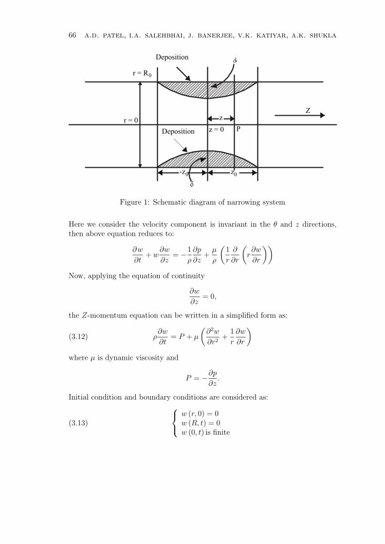
66 a.d. patel, i.a. salehbhai, j. banerjee, v.k. katiyar, a.k. shuklaz = 0
-z r = R
r = 0
Z
0
0 z0
Deposition
Deposition
z
P
Figure 1: Schematic diagram of narrowing system
Here we consider the velocity component is invariant in the θ and z directions,then above equation reduces to:
∂w
∂t+ w
∂w
∂z= −1
ρ
∂p
∂z+
µ
ρ
(1
r
∂
∂r
(r∂w
∂r
))
Now, applying the equation of continuity
∂w
∂z= 0,
the Z-momentum equation can be written in a simplified form as:
(3.12) ρ∂w
∂t= P + µ
(∂2w
∂r2+
1
r
∂w
∂r
)
where µ is dynamic viscosity and
P = −∂p
∂z.
Initial condition and boundary conditions are considered as:
(3.13)
w (r, 0) = 0w (R, t) = 0w (0, t) is finite
an analytical solution of fluid flow... 67
4. Solution of the problem
The method of integral transform is used to obtain the solution of the problem.Let
(4.14) w (λn, t) = H0 (w (r, t)) =
R∫
0
rw (r, t) J0 (rλn) dr
where λn are the roots of the equation J0 (Rλn) = 0. Also, by using the recurrencerelation of the Bessel function, we have
(4.15)
R∫
0
rJ0 (rλn) dr =R
λn
J1 ((Rλn) .
By taking the zero order finite Hankel transform (2.8) of (3.12) and using (4.14),(4.15) & (3,13) , yields
(4.16) ρ∂w
∂t=
PRJ1 (Rλn)
λn
− µλ2nw.
Let
(4.17) ˜w (λn, s) = L w (λn, t) =
∞∫
0
e−stw (λn, t) dt.
Also,
(4.18)
∞∫
0
e−stdt =1
s.
By taking the Laplace transform (2.6) of (4.16) and using (4.17), (4.18) & (3.13),we get
ρs ˜w (s) =PRJ1 (Rλn)
λns− µλ2
n˜w.
Further simplification gives
(4.19) ˜w =PRJ1 (Rλn)
(ρs + µλ2n) λns
.
Now, taking the inverse Laplace transform of this equation, gives
w =PRJ1 (Rλn)
λnρL−1
1
s(s + µ
ρλ2
n
) .
Now, using Convolution theorem (Debnath [8]), we have
w =PRJ1 (Rλn)
λnρ
t∫
0
L−1
1(s + µ
ρλ2
n
) , u
du,
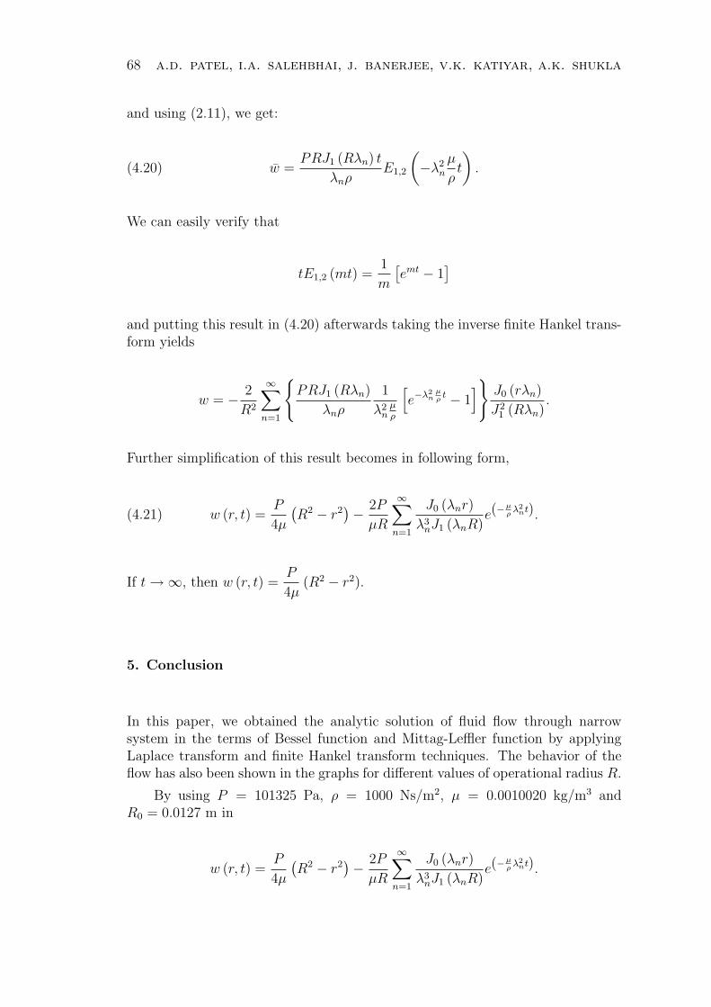
68 a.d. patel, i.a. salehbhai, j. banerjee, v.k. katiyar, a.k. shukla
and using (2.11), we get:
(4.20) w =PRJ1 (Rλn) t
λnρE1,2
(−λ2
n
µ
ρt
).
We can easily verify that
tE1,2 (mt) =1
m
[emt − 1
]
and putting this result in (4.20) afterwards taking the inverse finite Hankel trans-form yields
w = − 2
R2
∞∑n=1
PRJ1 (Rλn)
λnρ
1
λ2n
µρ
[e−λ2
nµρ
t − 1] J0 (rλn)
J21 (Rλn)
.
Further simplification of this result becomes in following form,
(4.21) w (r, t) =P
4µ
(R2 − r2
)− 2P
µR
∞∑n=1
J0 (λnr)
λ3nJ1 (λnR)
e(−µρ
λ2nt).
If t →∞, then w (r, t) =P
4µ(R2 − r2).
5. Conclusion
In this paper, we obtained the analytic solution of fluid flow through narrowsystem in the terms of Bessel function and Mittag-Leffler function by applyingLaplace transform and finite Hankel transform techniques. The behavior of theflow has also been shown in the graphs for different values of operational radius R.
By using P = 101325 Pa, ρ = 1000 Ns/m2, µ = 0.0010020 kg/m3 andR0 = 0.0127 m in
w (r, t) =P
4µ
(R2 − r2
)− 2P
µR
∞∑n=1
J0 (λnr)
λ3nJ1 (λnR)
e(−µρ
λ2nt).
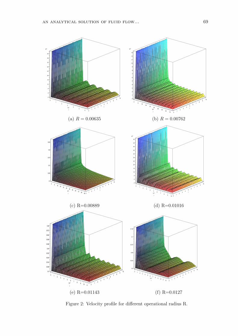
an analytical solution of fluid flow... 69
109
0 8
0
4
71
8
12
16
62
20
t
24
5
28
r
3
10 -3
32
4
36
40
4 3
10-4
25 16 0
109
0 8
0
1
8
2
7
3
4
16
5
6
6
24
7
t
8
532
9
r
10
10-4
11
440
12
13
48 3
10-3
56 264 1
72 0
(a) R = 0.00635 (b) R = 0.00762
1090
0.0
88
0.005
716
0.01
24 6
0.015
32
t
5
r
40
0.02
10-4
448
0.025
56 364 272 180 88 0
109
0 8
0
1
4
8
7
12
2
16
6
20
3
24
t
28
54
32
r
10 -3
36
5 4
40
44
6
48
37
10-3
28 1910 0
(c) R=0.00889 (d) R=0.01016
109
0
0.0
18
0.008
0.016
2
0.024
73
0.032
0.04
64
0.048
r
0.056
55
10-3
0.064
t6
0.072
4
0.08
7 38 9
210
111 0
109
0 8
0.0
1 72
0.025
3 6
0.05
4
t
5
0.075
5
r
10 -3
6
0.1
47
0.125
8 39 210 11 1
12 0
(e) R=0.01143 (f) R=0.0127
Figure 2: Velocity profile for different operational radius R.

70 a.d. patel, i.a. salehbhai, j. banerjee, v.k. katiyar, a.k. shukla
References
[1] Murlidhar, K. and Gautam Biswas, Advanced engineering fluid me-chanics, Narosa Publications, 2005.
[2] Verma, V.K., Katiyar, V.K. and Singh, M.P., Effect of multiple steno-sis on blood flow through a tube, Journal of Natural and physical sciences,2007.
[3] Verma, V.K., Singh, M.P. and Katiyar, V.K., Analytical study ofblood flow through an artery with mild stenosis, Acta Ciencia Indica, vol.XXX M, 2 (281), 2004.
[4] Ponalagusamy, R., Blood flow through an artery with mild stenosis: Atwo layered model, different shapes of stenosis and slip velocity at the wall,Journal of Applied Sciences, 7 (7) (2007), 1071.
[5] Chaturani, P. and Kaloni, P.N., Two-layered poiseuille flow model forblood flow through arteries of small diameter and arterioles, Biorehology, 13(1976), 243-250.
[6] Chaturani, P. and Upadhya, V.S., A two-layered model for blood flowthrough small diameter tubes, Biorehology, 16 (1979), 109-118.
[7] Chaturani, P. and Biswas, D., A theoretical study of blood flow throughstenoded arteries with velocity slip at the wall, Proc. First Internat Sympo-sium on Physiological Fluid Dynamics, IIT Madras, India, 1983, 23-26.
[8] Debnath, L., Integral Transforms and their Applications, CRC Press, NewYork-London-Tokyo, 1995.
[9] Rainville, E.D., Special Functions, The Macmillan Company, New York,1960.
[10] Mittag-Leffler, G.M., Sur la nouvelle fonction Eα(x), C.R. Acad. Sci.Paris, 137 (1903), 554-558.
[11] Wiman, A., Uber den fundamental Satz in der Theorie der FunktionenEα(x), Acta Math., 29 (1905), 191-201.
[12] Shukla, A.K. and Prajapati, J.C., On a generalization of Mittag–Lefflerfunction and its properties, J. Math. Anal. Appl., 336 (2007), 797-811.
Accepted: 12.09.2009
italian journal of pure and applied mathematics – n. 29−2012 (71−86) 71
ON GENERALIZED HILBERT ALGEBRAS
R.A. Borzooei
Department of MathematicsUniversity of Shahid BeheshtiTehranIrane-mail: [email protected]
J. Shohani
Department of MathematicsSistan and Balushestan UniversityZahedanIran
Abstract. In this paper by considering the notion of generalized Hilbert algebra whichis named g-Hilbert algebra, we obtain some properties of it. Moreover, we show that forall n ≥ 3 there exist at least one proper g-Hilbert algebra of order n. Because g-Hilbertalgebra is not a Boolean algebra we define the concept of branch in g-Hilbert algebrasand we prove that any branch in commutative g-Hilbert algebras is a Boolean algebra.
Keywords: generalized Hilbert algebra, implication algebras, complemented lattice,distributive lattice, Boolean algebra.
AMS Subject Classification (2000): 06F35, 03G25, 08A30.
1. Introduction
Hilbert algebras [7] represent the algebraic counterpart of the implicative fragmentof Intuitionistic Propositional Logic. In [7] Diego gives a topological representa-tion for Hilbert algebras and he proves that every Hilbert algebra is isomorphicto a subalgebra of the implicative reduct of a Heyting algebra generated by acertain topological space. Also, Hilbert algebras, or positive implication algebras[14], are the duals of Henkin algebras called by him implicative models in [9].Positive implicative BCK-algebras [11] are actually another version of Henkin al-gebras. As a matter of fact, these algebras are an algebraic counterpart of positiveimplicational calculus. Various expansions of Hilbert algebras by a conjunction-like operation have also been studied in the literature. The most extensivelyinvestigated among them are implicative semilattices, which are known also asBrouwerian semilattices.
72 r.a. borzooei, j. shohani
Now, in this paper we give a generalization of positive implicative BCK-algebras and Hilbert algebras which is called a generalized Hilbert algebra that itis in form of variety. In follow, we obtain some properties of generalized Hilbertalgebra and we show that any branch in commutative generalized Hilbert algebrasis a Boolean algebra.
2. Generalized Hilbert algebras
Definition 2.1. [7] A Hilbert algebra is a triplet (H,→, 1) of type (2,0), where His a nonempty set, “→” is a binary operation which satisfies the following axioms:
(H1) x → (y → x) = 1,
(H2) (x → (y → z)) → ((x → y) → (x → z)) = 1,
(H3) x → y = 1 and y → x = 1 imply x = y,
for all x, y, z ∈ H.
Proposition 2.2. [8] If (H,→, 1) be a Hilbert algebra, then,
(i) x → x = 1,
(ii) 1 → x = x,
(iii) x → 1 = 1,
(iv) x → (y → z) = y → (x → z),
(v) x → (y → z) = (x → y) → (x → z),
for all x, y, z ∈ H.
Definition 2.3. A generalized Hilbert algebra (or briefly, g-Hilbert algebra) is analgebra (GH ,→, 1) of type (2,0) which satisfies the following axioms;
(GH1) 1 → x = x,
(GH2) x → x = 1,
(GH3) z → (y → x) = y → (z → x),
(GH4) z → (y → x) = (z → y) → (z → x),
for all x, y, z ∈ GH .
Example 2.4. Let (X,≤, 1) be a unital poset and implication ” → ” on X isdefined as follows:
x → y =
1, if x ≤ y,
y, otherwise.
Then (X,→, 1) is a g-Hilbert algebra.
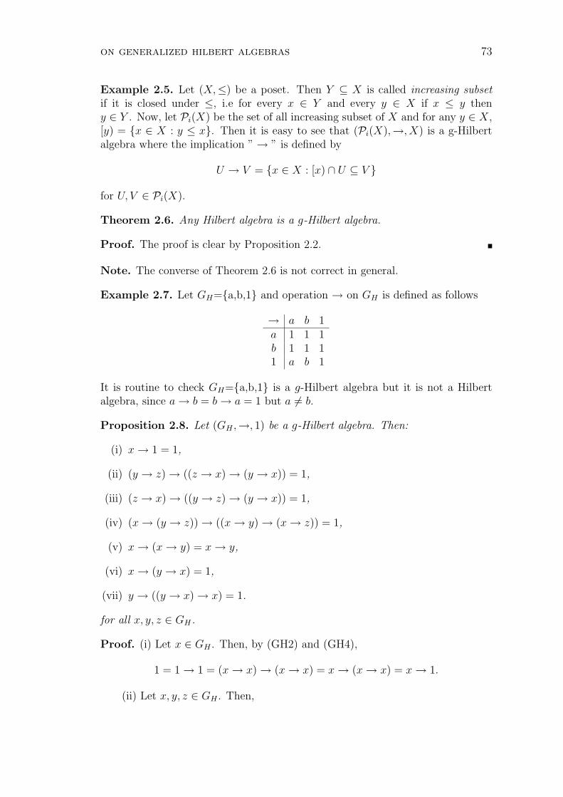
on generalized hilbert algebras 73
Example 2.5. Let (X,≤) be a poset. Then Y ⊆ X is called increasing subsetif it is closed under ≤, i.e for every x ∈ Y and every y ∈ X if x ≤ y theny ∈ Y . Now, let Pi(X) be the set of all increasing subset of X and for any y ∈ X,[y) = x ∈ X : y ≤ x. Then it is easy to see that (Pi(X),→, X) is a g-Hilbertalgebra where the implication ” → ” is defined by
U → V = x ∈ X : [x) ∩ U ⊆ V
for U, V ∈ Pi(X).
Theorem 2.6. Any Hilbert algebra is a g-Hilbert algebra.
Proof. The proof is clear by Proposition 2.2.
Note. The converse of Theorem 2.6 is not correct in general.
Example 2.7. Let GH=a,b,1 and operation → on GH is defined as follows
→ a b 1a 1 1 1b 1 1 11 a b 1
It is routine to check GH=a,b,1 is a g-Hilbert algebra but it is not a Hilbertalgebra, since a → b = b → a = 1 but a 6= b.
Proposition 2.8. Let (GH ,→, 1) be a g-Hilbert algebra. Then:
(i) x → 1 = 1,
(ii) (y → z) → ((z → x) → (y → x)) = 1,
(iii) (z → x) → ((y → z) → (y → x)) = 1,
(iv) (x → (y → z)) → ((x → y) → (x → z)) = 1,
(v) x → (x → y) = x → y,
(vi) x → (y → x) = 1,
(vii) y → ((y → x) → x) = 1.
for all x, y, z ∈ GH .
Proof. (i) Let x ∈ GH . Then, by (GH2) and (GH4),
1 = 1 → 1 = (x → x) → (x → x) = x → (x → x) = x → 1.
(ii) Let x, y, z ∈ GH . Then,

74 r.a. borzooei, j. shohani
(y → z) → ((z → x) → (y → x))
= (z → x) → ((y → z) → (y → x)), (by (GH3))
= (z → x) → (y → (z → x)), (by (GH4))
= y → ((z → x) → (z → x)), (by (GH3))
= y → 1, (by (GH2))
= 1 (by (i)).
(iii) Let x, y, z ∈ GH . Then by (GH3) and (ii);
(z → x) → ((y → z) → (y → x)) = (y → z) → ((z → x) → (y → x)) = 1.
(iv) Let x, y, z ∈ GH . Then by (GH4) and (GH2);
(x → (y → z)) → ((x → y) → (x → z))
= ((x → y) → (x → z)) → ((x → y) → (x → z)) = 1.
(v) Let x, y, z ∈ GH . Then by (GH4) and (GH1);
x → (x → y) = (x → x) → (x → y) = 1 → (x → y) = x → y.
(vi) Let x, y, z ∈ GH . Then by (GH4) and (i);
x → (y → x) = (x → y) → (x → x) = (x → y) → 1 = 1.
(vii) Let x, y, z ∈ GH . Then by (GH3) and (GH2);
y → ((y → x) → x) = (y → x) → (y → x) = 1.
Definition 2.9. Let (GH ,→, 1) be a g-Hilbert algebra, then, GH is called a properg-Hilbert algebra if it is not a Hilbert algebra.
Proposition 2.10. If GH is a proper g-Hilbert algebra of order n, then n ≥ 3.
Proof. By Definition 2.3, Proposition 2.8 and Example 2.7, the proof is clear.
Theorem 2.11. Let (GH ,→, 1) be a proper g-Hilbert algebra and a 6∈ GH . ThenG′H = GH ∪ a with the following operation is a proper g-Hilbert algebra.
x → y =
x → y , x, y ∈ GH ,
a , x = 1, y = a,
1 , x ∈ G′H − 1, y = a,
y , x = a, y ∈ GH .
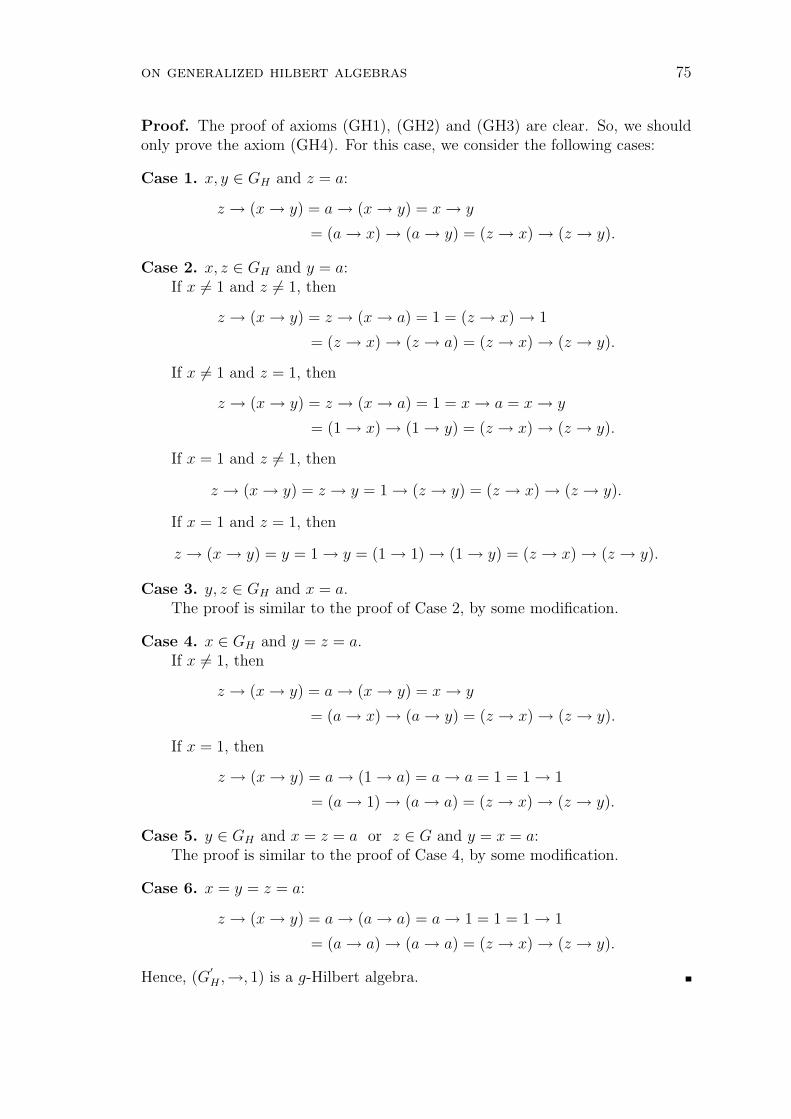
on generalized hilbert algebras 75
Proof. The proof of axioms (GH1), (GH2) and (GH3) are clear. So, we shouldonly prove the axiom (GH4). For this case, we consider the following cases:
Case 1. x, y ∈ GH and z = a:
z → (x → y) = a → (x → y) = x → y
= (a → x) → (a → y) = (z → x) → (z → y).
Case 2. x, z ∈ GH and y = a:If x 6= 1 and z 6= 1, then
z → (x → y) = z → (x → a) = 1 = (z → x) → 1
= (z → x) → (z → a) = (z → x) → (z → y).
If x 6= 1 and z = 1, then
z → (x → y) = z → (x → a) = 1 = x → a = x → y
= (1 → x) → (1 → y) = (z → x) → (z → y).
If x = 1 and z 6= 1, then
z → (x → y) = z → y = 1 → (z → y) = (z → x) → (z → y).
If x = 1 and z = 1, then
z → (x → y) = y = 1 → y = (1 → 1) → (1 → y) = (z → x) → (z → y).
Case 3. y, z ∈ GH and x = a.The proof is similar to the proof of Case 2, by some modification.
Case 4. x ∈ GH and y = z = a.If x 6= 1, then
z → (x → y) = a → (x → y) = x → y
= (a → x) → (a → y) = (z → x) → (z → y).
If x = 1, then
z → (x → y) = a → (1 → a) = a → a = 1 = 1 → 1
= (a → 1) → (a → a) = (z → x) → (z → y).
Case 5. y ∈ GH and x = z = a or z ∈ G and y = x = a:The proof is similar to the proof of Case 4, by some modification.
Case 6. x = y = z = a:
z → (x → y) = a → (a → a) = a → 1 = 1 = 1 → 1
= (a → a) → (a → a) = (z → x) → (z → y).
Hence, (G′H ,→, 1) is a g-Hilbert algebra.
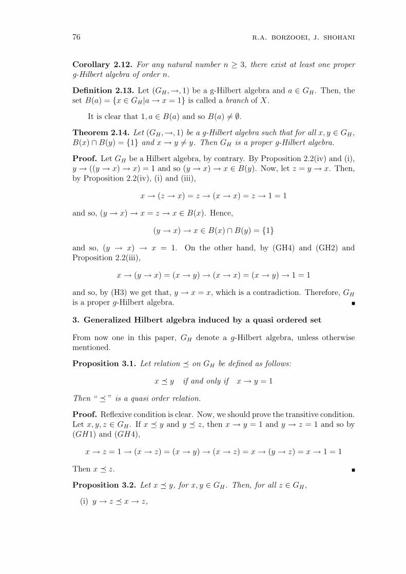
76 r.a. borzooei, j. shohani
Corollary 2.12. For any natural number n ≥ 3, there exist at least one properg-Hilbert algebra of order n.
Definition 2.13. Let (GH ,→, 1) be a g-Hilbert algebra and a ∈ GH . Then, theset B(a) = x ∈ GH |a → x = 1 is called a branch of X.
It is clear that 1, a ∈ B(a) and so B(a) 6= ∅.Theorem 2.14. Let (GH ,→, 1) be a g-Hilbert algebra such that for all x, y ∈ GH ,B(x) ∩B(y) = 1 and x → y 6= y. Then GH is a proper g-Hilbert algebra.
Proof. Let GH be a Hilbert algebra, by contrary. By Proposition 2.2(iv) and (i),y → ((y → x) → x) = 1 and so (y → x) → x ∈ B(y). Now, let z = y → x. Then,by Proposition 2.2(iv), (i) and (iii),
x → (z → x) = z → (x → x) = z → 1 = 1
and so, (y → x) → x = z → x ∈ B(x). Hence,
(y → x) → x ∈ B(x) ∩B(y) = 1
and so, (y → x) → x = 1. On the other hand, by (GH4) and (GH2) andProposition 2.2(iii),
x → (y → x) = (x → y) → (x → x) = (x → y) → 1 = 1
and so, by (H3) we get that, y → x = x, which is a contradiction. Therefore, GH
is a proper g-Hilbert algebra.
3. Generalized Hilbert algebra induced by a quasi ordered set
From now one in this paper, GH denote a g-Hilbert algebra, unless otherwisementioned.
Proposition 3.1. Let relation ¹ on GH be defined as follows:
x ¹ y if and only if x → y = 1
Then “ ¹ ” is a quasi order relation.
Proof. Reflexive condition is clear. Now, we should prove the transitive condition.Let x, y, z ∈ GH . If x ¹ y and y ¹ z, then x → y = 1 and y → z = 1 and so by(GH1) and (GH4),
x → z = 1 → (x → z) = (x → y) → (x → z) = x → (y → z) = x → 1 = 1
Then x ¹ z.
Proposition 3.2. Let x ¹ y, for x, y ∈ GH . Then, for all z ∈ GH ,
(i) y → z ¹ x → z,
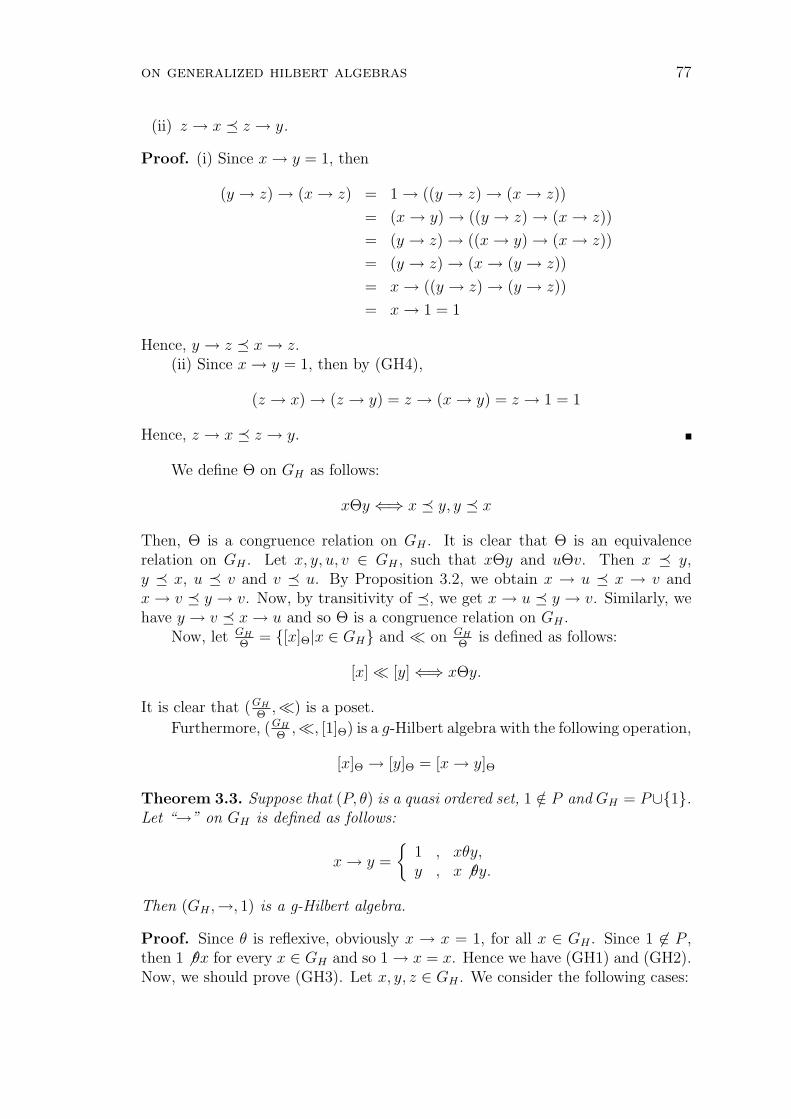
on generalized hilbert algebras 77
(ii) z → x ¹ z → y.
Proof. (i) Since x → y = 1, then
(y → z) → (x → z) = 1 → ((y → z) → (x → z))
= (x → y) → ((y → z) → (x → z))
= (y → z) → ((x → y) → (x → z))
= (y → z) → (x → (y → z))
= x → ((y → z) → (y → z))
= x → 1 = 1
Hence, y → z ¹ x → z.(ii) Since x → y = 1, then by (GH4),
(z → x) → (z → y) = z → (x → y) = z → 1 = 1
Hence, z → x ¹ z → y.
We define Θ on GH as follows:
xΘy ⇐⇒ x ¹ y, y ¹ x
Then, Θ is a congruence relation on GH . It is clear that Θ is an equivalencerelation on GH . Let x, y, u, v ∈ GH , such that xΘy and uΘv. Then x ¹ y,y ¹ x, u ¹ v and v ¹ u. By Proposition 3.2, we obtain x → u ¹ x → v andx → v ¹ y → v. Now, by transitivity of ¹, we get x → u ¹ y → v. Similarly, wehave y → v ¹ x → u and so Θ is a congruence relation on GH .
Now, let GH
Θ= [x]Θ|x ∈ GH and ¿ on GH
Θis defined as follows:
[x] ¿ [y] ⇐⇒ xΘy.
It is clear that (GH
Θ,¿) is a poset.
Furthermore, (GH
Θ,¿, [1]Θ) is a g-Hilbert algebra with the following operation,
[x]Θ → [y]Θ = [x → y]Θ
Theorem 3.3. Suppose that (P, θ) is a quasi ordered set, 1 /∈ P and GH = P∪1.Let “→” on GH is defined as follows:
x → y =
1 , xθy,y , x 6 θy.
Then (GH ,→, 1) is a g-Hilbert algebra.
Proof. Since θ is reflexive, obviously x → x = 1, for all x ∈ GH . Since 1 6∈ P ,then 1 6 θx for every x ∈ GH and so 1 → x = x. Hence we have (GH1) and (GH2).Now, we should prove (GH3). Let x, y, z ∈ GH . We consider the following cases:
78 r.a. borzooei, j. shohani
Case 1. y 6 θx and z 6 θx:
z → (y → x) = z → x = x = y → x = y → (z → x).
Case 2. yθx and z 6 θx:
z → (y → x) = z → 1 = 1 = y → x = y → (z → x).
Case 3. y 6 θx and zθx:
z → (y → x) = z → x = 1 = y → 1 = y → (z → x).
Case 4. yθx and zθx:
z → (y → x) = z → 1 = 1 = y → 1 = y → (z → x).
Hence, we have (GH3).Now, we will prove (GH4). Let x, y, z ∈ GH . Then, we consider the following
cases:
Case 1. zθy and zθx:If xθy, then:
(z → y) → (z → x) = 1 → 1 = 1 = z → 1 = z → (y → x).
If x 6 θy, then:
(z → y) → (z → x) = 1 → 1 = 1 = z → x = z → (y → x).
Case 2. z 6 θy and zθx:If xθy, then:
(z → y) → (z → x) = y → 1 = 1 = z → 1 = z → (y → x).
If x 6 θy, then:
(z → y) → (z → x) = y → 1 = 1 = z → x = z → (y → x).
Case 3. zθy and z 6 θx:If xθy, then by transitive condition zθx, which is not impossible.If x 6 θy, then:
(z → y) → (z → x) = 1 → x = x = z → x = z → (y → x).
Case 4. z 6 θy and z 6 θx:If xθy, then:
(z → y) → (z → x) = y → x = 1 = z → 1 = z → (y → x).
on generalized hilbert algebras 79
If x 6 θy, then
(z → y) → (z → x) = y → x = x = z → x = z → (y → x).
Hence, we have (GH4). Therefore, GH is a g-Hilbert algebra.
4. Relation between generalized Hilbert algebras and implicationalgebras
Definition 4.1. [1] An implication algebra is a set X with a binary operation“→” which satisfies the following axioms:
(I1) (x → y) → x = x,
(I2) (x → y) → y = (y → x) → x,
(I3) x → (y → z) = y → (x → z),
for all x, y, z ∈ X.In any implication algebra (X,→), we have
(I4) x → (x → y) = x → y,
(I5) x → x = y → y,
(I6) there exists a unique element 1 in X such that, for all x ∈ X,
(a) x → x = 1, 1 → x = x and x → 1 = 1,
(b) if x → y = 1 and y → x = 1 then x = y,
(c) x → (y → x) = 1
for all x, y ∈ X.
Definition 4.2. GH is called commutative if for all x, y ∈ GH ,
(y → x) → x = (x → y) → y.
Lemma 4.3. Let GH be commutative. If x → y = y → x = 1, then x = y.
Proof. Let x → y = y → x = 1, for x, y ∈ G. Since GH is commutative, then by(GH1),
x = 1 → x = (y → x) → x = (x → y) → y = 1 → y = y.
Lemma 4.4. [1] Let (X,→, 1) be an implication algebra. Then,
(i) x ≤ y, imply y → z ≤ x → z
(ii) x ≤ y, imply z → x ≤ z → y
(iii) x → y ≤ (y → z) → (x → z) and y → z ≤ (x → y) → (x → z).
80 r.a. borzooei, j. shohani
Theorem 4.5. (X,→, 1) is an implication algebra if and only if (X,→, 1) is acommutative g-Hilbert algebra.
Proof. (⇒) Let (X,→, 1) be an implication algebra. By Theorem 2.6, it isenough to prove that X is a Hilbert algebra. By (I6)(b) and (c), we have (H1)and (H3). It is enough to prove (H2). Let x, y, z ∈ X. Then, by (I4), (I3) andLemma 4.4,
(x → (y → z)) → ((x → y) → (x → z))
= (x → (y → z)) → ((x → y) → (x → (x → z))),
≥ (x → (y → z)) → (y → (x → z))),
= (x → (y → z)) → (x → (y → z))),
= 1.
Hence, by (I6)(a),(b), we have (x → (y → z)) → ((x → y) → (x → z))) = 1, andso (H2) is hold. Hence, (X,→, 1) is a Hilbert algebra and so, by Theorem 2.6, itis a g-Hilbert algebra. Moreover, by (I2) it is commutative.
(⇐) Let (X,→, 1) be a commutative g-Hilbert algebra. Since X is commu-tative, then we have (I2). Moreover, by (GH3), we have (I3). Now, it is enoughto prove that (I1). Let x, y ∈ X. Then, by (GH3), (GH2) and Proposition 2.8(i),
x → ((x → y) → x) = (x → y) → (x → x) = (x → y) → 1 = 1
Hence,
(1) x → ((x → y) → x) = 1.
Moreover,
((x → y) → x) → x = (x → (x → y)) → (x → y), Since X is commutative
= ((x → x) → (x → y)) → (x → y), by (GH4)
= (1 → (x → y)) → (x → y), by (GH2)
= (x → y) → (x → y)
= 1.
Hence,
(2) ((x → y) → x) → x = 1,
and so, by (1), (2) and Lemma 4.3 we have (I1). Therefore, (X,→, 1) is animplication algebra.
Example 4.6. Let GH = a, b, c, 1 and operation “→” on GH is defined asfollows:
→ a b c 1a 1 1 1 1b 1 1 1 1c 1 1 1 11 a b c 1
on generalized hilbert algebras 81
Then, (GH ,→, 1) is a g-Hilbert algebra which is not an implication algebra, since(b → c) → c 6= (c → b) → b. Hence, a commutative condition is necessary in thelast theorem.
5. Lattice structure on commutative generalized Hilbert algebras
Proposition 5.1. If GH is commutative, then
(i) (x → y) → x = x,
(ii) x → (x → y) = x → y,
for all x, y ∈ GH .
Proof. (i) Let x, y ∈ GH . Then,
x → ((x → y) → x) = (x → (x → y)) → (x → x), (by (GH4))
= (x → (x → y)) → 1, (by (GH2))
= 1
On the other hand,
((x → y) → x) → x = (x → (x → y)) → (x → y), (since GH is commutative)
= ((x → x) → (x → y)) → (x → y), (by (GH4))
= (1 → (x → y)) → (x → y), (by (GH2))
= (x → y) → (x → y), (by (GH1))
= 1 (by (GH2)).
Hence, by Lemma 4.3 we obtain (x → y) → x = x.(ii) By using (i) twice, we have
x → (x → y) = ((x → y) → x) → (x → y) = x → y.
Corollary 5.2. Let GH be commutative and relation ¹ on GH , is defined by x ¹ yif and only if x → y = 1. Then, “ ¹ ” is a partial order on GH .
Proof. By (GH2), Proposition 5.1(i) we get that ¹ is reflexive and anti symmet-ric. Let x → y = 1 and y → z = 1, then
x → z = 1 → (x → z) = (x → y) → (x → z) = x → (y → z) = x → 1 = 1.
Thus, ¹ is a partial order on GH .
Proposition 5.3. For any p ∈ GH , B(p) is a subalgebra of GH .
Proof. It is clear that 1 ∈ B(p). Now, let a, b ∈ B(p). Then, p ¹ a and p ¹ band so by (GH4)and (GH2),
p → (a → b) = (p → a) → (p → b) = 1 → 1 = 1.
Hence, p ¹ (a → b) and so a → b ∈ B(p). Therefore, B(p) is a subalgebra of GH .
82 r.a. borzooei, j. shohani
Theorem 5.4. If GH is commutative, then the following are hold:
(i) (GH ,∨) is a ∨−semi lattice, when a ∨ b = (a → b) → b, for any a, b ∈ GH ,
(ii) For any p ∈ GH , (B(p),∧) is a ∧−semi lattice, when a ∧ b = ((a → p) ∨(b → p)) → p, for any a, b ∈ B(p),
(iii) For any p ∈ GH , (B(p),∧,∨) is a complemented lattice.
Proof. By Corollary 5.2, (GH ,¹) and so (B(p),¹), for any p ∈ GH is a partialordered set. (i) Let a, b ∈ GH . First we should prove that (a → b) → b is anupper bound of a, b. By (GH3) and (GH2), a → ((a → b) → b) = (a → b) →(a → b) = 1, and so a ¹ (a → b) → b. Moreover, by (GH3), b ¹ (a → b) → b.Hence, (a → b) → b is an upper bound of a, b. Now, let c ∈ G such that a, b ¹ c.Then a → c = 1 and so by commutative condition and (GH1),
(1) (c → a) → a = (a → c) → c = 1 → c = c.
Hence,
((a → b) → b) → c
= ((a → b) → b) → ((c → a) → a), (by (1))
= (c → a) → (((a → b) → b) → a), (by (GH3))
= (c → a) → (((b → a) → a) → a), (by commutative condition)
= (c → a) → ((a → (b → a)) → (b → a)), (by commutative condition)
= (c → a) → ((b → (a → a)) → (b → a)), (by (GH3))
= (c → a) → ((b → 1) → (b → a)), (by (GH2))
= (c → a) → (1 → (b → a)), (by Proposition 2.8(i))
= (c → a) → (b → a), (by (GH1))
= b → ((c → a) → a), (by (GH3))
= b → c, (by (1))
= 1 (since b ¹ c).
Therefore, (a → b) → b ¹ c and so a ∨ b = (a → b) → b. Hence, (GH ,∨) is a∨−semi lattice.
(ii) Let p ∈ GH and a, b ∈ B(p). Then p ¹ a, b.Since a → p ¹ (a → p)∨(b → p) then, by Proposition 3.2,
((a → p) ∨ (b → p)) → p ¹ (a → p) → p = a ∨ p = a.
Similarly, we can prove that ((a → p) ∨ (b → p)) → p ¹ b. Hence, ((a → p)∨ (b → p)) → p is a lower bound of a and b. Now, let c ∈ GH such thatc ¹ a, b. Then, by Proposition 3.2, a → p ¹ c → p and b → p ¹ c → p and so((a → p) ∨ (b → p)) ¹ c → p. Hence, by Proposition 3.2, c ¹ c ∨ p = (c → p) →
on generalized hilbert algebras 83
p ¹ [a → p) ∨ (b → p)] → p. Therefore, ((a → p) ∨ (b → p)) → p is a greatestlower bound of a and b and so
a ∧ b = ((a → p) ∨ (b → p)) → p.
Now, since a ∧ b ∈ B(p), then (B(p),∧) is a ∧−semilattice.
(iii) Let p ∈ GH . Then, for any a ∈ B(p),
(a → p) ∨ a = ((a → p) → a) → a
= (a → (a → p)) → (a → p), (by commutative condition)
= (a → p) → (a → p), (by Proposition 2.8(v))
= 1, (by (GH2))
Moreover, by commutative condition,
a ∧ (a → p) = ((a → p) ∨ ((a → p) → p)) → p
= ((a → p) ∨ ((p → a) → a)) → p
= ((a → p) ∨ (p ∨ a)) → p
= (a → p) ∨ a) → p
= 1 → p
= p
Therefore, (B(p),∧,∨) is a complemented lattice.
Lemma 5.5. Let GH be a commutative g-Hilbert algebra and p ∈ GH . Then, forany a, b ∈ B(p),
(a → p) ∨ (b → p) = (a ∧ b) → p.
Proof. Let p ∈ GH and a, b ∈ B(p). Since a ∧ b ¹ a and a ∧ b ¹ b, then, byProposition 3.2, a → p ¹ (a∧b) → p and b → p ¹ (a∧b) → p and so (a∧b) → p isan upper bound of a → p and b → p. Now, let u ∈ B(p) be an other upper boundof a → p and b → p. Then, a → p ¹ u and b → p ¹ u and so, by Proposition 3.2,u → p ¹ (a → p) → p and u → p ¹ (b → p) → p. Hence, u → p ¹ a ∨ p = a andu → p ¹ b ∨ p = b and so u → p ¹ a ∧ b. Thus,
a ∧ b → p ¹ (u → p) → p = u ∨ p = u
Therefore, a ∧ b → p is last upper bound of a → p and b → p, that is,
(a → p) ∨ (b → p) = (a ∧ b) → p.
Theorem 5.6. If GH is commutative, then for any p ∈ GH , (B(p),∨,∧) is adistributive lattice.
84 r.a. borzooei, j. shohani
Proof. Let p ∈ GH and a, b, c ∈ B(p). We have to prove that a ∧ (b ∨ c) =(a∧ b)∨ (a∧ c). Since p ¹ b, then by Proposition 3.2, a → p ¹ a → b. Moreover,by Proposition 2.8(vi), b ¹ a → b and so (a → p)∨b ¹ a → b. Let c = (a → p)∨b.Then
(1) c ¹ a → b and b ¹ c and so c = b ∨ c = (c → b) → b.
Moreover, by the proof of Theorem 5.4(iii),
(2) (a → c) → c = a ∨ c = a ∨ (a → p) ∨ b = 1 ∨ b = 1.
Moreover,
(a → b) → c = (a → b) → (1 → c), (by (GH1))
= (a → b) → (((a → c) → c) → c), (by (2))
= (a → b) → ((a → c) ∨ c),
= (a → b) → (a → c), (by Proposition 2.8(vi))
= (a → b) → (a → ((c → b) → b), (by (1))
= (a → b) → ((c → b) → (a → b)), (by (GH3))
= (c → b) → ((a → b) → (a → b)), (by (GH3))
= (c → b) → 1, (by (GH1))
= 1.
and this implies that a → b ¹ c. Hence, by (1) and Proposition 5.1(i),
(2) a → b = c = (a → p) ∨ b.
Now, since (2) holds for any a, b ∈ B(p) and since B(p) is a subalgebra, thena, b → p ∈ B(p) and so, by (2),
(3) (a → (b → p)) → p = ((a → p) ∨ (b → p)) → p = a ∧ b.
Hence,
a → (a ∧ b) = a → ((a → (b → p)) → p), (by (3))
= (a → (b → p)) → (a → p), (by Proposition 2.8(v))
= (b → (a → p)) → (a → p), (by (GH3))
= b ∨ (a → p),
= a → b, (by (2))
and this implies that
(4) a → (a ∧ b) = a → b.
Now, let k = (a ∧ b) ∨ (a ∧ c). Since, a ∧ b ¹ k, then by Proposition 3.2, (GH1),(GH2), (GH3) and (4),
1 = a → 1 = a → (b → b) = b → (a → b) = b → (a → (a ∧ b)) ¹ b → (a → k)
on generalized hilbert algebras 85
and so, by Proposition 2.8(i), b → (a → k) = 1 and this implies that b ¹ a → k.Similarly, c ¹ a → k and so
(5) b ∨ c ¹ a → k.
and, by Proposition 3.2,
(6) (a → k) → k ¹ (b ∨ c) → k.
Now, since a∧b ¹ a and a∧c ¹ a, then k = (a∧b)∨(a∧c) ¹ a and so k → a = 1.Hence, by (6) and the commutative condition,
(7) a = 1 → a = (k → a) → a = (a → k) → k ¹ (b ∨ c) → k.
Hence, by (5), (7) and the commutative property,
(a → k) ∨ ((b ∨ c) → k) º (a → k) ∨ a = ((a → k) → a) → a = a → a = 1.
Now, since (a → k) ∨ ((b ∨ c) → k) ¹ 1, then, by Proposition 5.1(i),
(8) (a → k) ∨ (b ∨ c) → k) = 1.
Moreover, since a ∧ b ¹ b ∨ c and a ∧ c ¹ b ∨ c, then k = (a ∧ b) ∨ (a ∧ c) ¹ b ∨ c.Now, since we proved that k ¹ a. Hence by (8),
a ∧ (b ∨ c) = ((a → k) ∨ ((b ∨ c) → k)) → k = 1 → k = k = (a ∧ b) ∨ (a ∧ c).
Therefore, (B(p),∧,∨) is a distributive Lattice.
Corollary 5.7. If GH is commutative, then for any p ∈ GH , (B(p),∨,∧) is aBoolean lattice.
Proof. By Theorems 5.4 and 5.6, the proof is clear.
References
[1] Abbott, J.C., Implicational algebras, Bull. Math R.S. Roumaine, 11 (1967),3-23.
[2] Abbott, J.C., Sets, lattices and boolean algebras, Allyn and Bacon, Boston,1969.
[3] Birkhoff, G., Lattice Theory, American Mathematical Society, ColloquiumPublications, XXV, 1940, third edition, 1967.
[4] Blyth, T.S., Lattices and Orderd Algebraic Structurres, Springer-Verlag,London, 2005.
86 r.a. borzooei, j. shohani
[5] Celani, S., Cabrer, L., Duality for finite Hilbert algebras, Discrete Ma-thematics, 305 (2005), 74-99.
[6] Chen, C.C., Gratzer, G., Stone lattices I. Construction theorems, CanadaJournal of Mathematics, 21 (1969), 884-894.
[7] Diego, A., Sur les alg‘ebres de Hilbert, Collection de LogiqueMath‘ematique, Serie A, 21, Gauthier-Villars, Paris, 1966.
[8] Halas, R., Remarks on commutative Hilbert algebras, Mathematica Bohe-mica, 4 (2002), 525-529.
[9] Henkin, L., An algebraic characterization of quantifiers, Fund. Math.,vol. 37, (1950), 6374.
[10] Imai, Y., Iseki, K., On axiom systems of propositional calculi, XIV Proc.Japan Academy, 42 (1966), 19-22.
[11] Iseki, K., Tanaka, S., An introduction to the theory of BCK-algebras,Mathematicae Japonicae, 23 (1978), 1-26.
[12] Cirulis, J., Hilbert algebras as implicative partial semilattices, Central Euro-pean Journal of Mathematics, 5(2) (2007), 264-279.
[13] Jun, Y.B., Deductive systems of Hilbert algebras, Scientiae MathematicaeJaponicae, 43 (1996), 51-54.
[14] Rasiwa, H., An algebraic approach to non-classical logics, Studies in logicand the foundations of mathematicas, 78, North-Holland, (1974).
Accepted: 07.11.2009
italian journal of pure and applied mathematics – n. 29−2012 (87−92) 87
mth POWER SYMMETRIC n-SIGRAPHS
R. Rangarajan
Department of Studies in MathematicsUniversity of MysoreManasagangotri, Mysore 570 006India
P. Siva Kota Reddy
Department of MathematicsAcharya Institute of TechnologySoladevanahalli, Bangalore-560 090Indiae-mail: reddy [email protected]
N.D. Soner
Department of Studies in MathematicsUniversity of MysoreManasagangotri, Mysore 570 006India
Abstract. An n-tuple (a1, a2, ..., an) is symmetric, if ak = an−k+1, 1 ≤ k ≤ n.A symmetric n-sigraph (symmetric n-marked graph) is an ordered pair Sn = (G, σ)(Sn = (G,µ)), where G = (V, E) is a graph called the underlying graph of Sn andσ : E → Hn (µ : V → Hn) is a function. The mth power graph of a graph G = (V, E)is a graph Gm = (V, E′), with same vertex set as G, and has two vertices u and vare adjacent if their distance in G is m or less. Analogously, one can define the mth
power symmetric n-sigraph Smn of a symmetric n-sigraph Sn = (G, σ) as a symmetric
n-sigraph, Smn = (Gm, σ′), where Gm is the underlying graph of Sm
n , and for any edgee = uv in Sm
n , σ′(e) = µ(u)µ(v), where for any v ∈ V ,
µ(v) =∏
u∈N(v)
σ(uv).
It is shown that for any symmetric n-sigraph Sn, its mth power symmetric n-sigraphSm
n is i-balanced. We then give structural characterization of mth power symmetricn-sigraphs. Further, we obtain some switching equivalence relationship between mth
power symmetric n-sigraph and line symmetric n-sigraph.
Keywords and phrases: symmetric n-sigraphs, symmetric n-marked graphs, balance,switching, mth power symmetric n-sigraph, line symmetric n-sigraphs, complementarysymmetric n-sigraphs, complementation.
2000 AMS Mathematics Subject Classification: 05C22.

88 r. rangarajan, p. siva kota reddy, n.d. soner
1. Introduction
For standard terminology and notion in graph theory we refer the reader to Harary[2]; the non-standard will be given in this paper as and when required. We treatonly finite simple graphs without self loops and isolates.
Let n≥1 be an integer. An n-tuple (a1, a2, ..., an) is symmetric if ak = an−k+1,1 ≤ k ≤ n. Let Hn = (a1, a2, ..., an) : ak ∈ +,−, ak = an−k+1, 1 ≤ k ≤ n bethe set of all symmetric n-tuples. Note that Hn is a group under coordinate wisemultiplication, and the order of Hn is 2m, where m = dn
2e.
A symmetric n-sigraph (symmetric n-marked graph) is an ordered pairSn = (G, σ) (Sn = (G,µ)), where G = (V,E) is a graph called the underlyinggraph of Sn and σ : E → Hn (µ : V → Hn) is a function.
In this paper by an n-tuple/n-sigraph/n-marked graph we always mean asymmetric n-tuple/symmetric n-sigraph/symmetric n-marked graph.
An n-tuple (a1, a2, ..., an) is the identity n-tuple, if ak = +, for 1 ≤ k ≤ n,otherwise it is a non-identity n-tuple. In an n-sigraph Sn = (G, σ) an edgelabelled with the identity n-tuple is called an identity edge, otherwise it is a non-identity edge.
Further, in an n-sigraph Sn = (G, σ), for any A ⊆ E(G) the n-tuple σ(A) isthe product of the n-tuples on the edges of A.
In [6], the authors defined two notions of balance in n-sigraph Sn = (G, σ) asfollows (see, also, R. Rangarajan and P. Siva Kota Reddy [3]):
Definition. Let Sn = (G, σ) be an n-sigraph. Then,
(i) Sn is identity balanced (or i-balanced), if product of n-tuples on each cycleof Sn is the identity n-tuple, and
(ii) Sn is balanced, if every cycle in Sn contains an even number of non-identityedges.
Note: An i-balanced n-sigraph need not be balanced and conversely.
The following characterization of i-balanced n-sigraphs is obtained in [6].
Proposition 1 (E. Sampathkumar et al. [6]) An n-sigraph Sn = (G, σ) isi-balanced if, and only if, it is possible to assign n-tuples to its vertices such thatthe n-tuple of each edge uv is equal to the product of the n-tuples of u and v.
In [6], the authors also have defined switching and cycle isomorphism of ann-sigraph Sn = (G, σ) as follows:
Let Sn = (G, σ) and S ′n = (G′, σ′), be two n-sigraphs. Then Sn and S ′n aresaid to be isomorphic, if there exists an isomorphism φ : G → G′ such that if uvis an edge in Sn with label (a1, a2, ..., an) then φ(u)φ(v) is an edge in S ′n with label(a1, a2, ..., an).
Given an n-marking µ of an n-sigraph Sn = (G, σ), switching Sn with res-pect to µ is the operation of changing the n-tuple of every edge uv of Sn by
mth power symmetric n-sigraphs 89
µ(u)σ(uv)µ(v). The n-sigraph obtained in this way is denoted by Sµ(Sn) and iscalled the µ-switched n-sigraph or just switched n-sigraph.
Further, an n-sigraph Sn switches to n-sigraph S ′n (or that they are switchingequivalent to each other), written as Sn ∼ S ′n, whenever there exists an n-markingof Sn such that Sµ(Sn) ∼= S ′n.
Two n-sigraphs Sn = (G, σ) and S ′n = (G′, σ′) are said to be cycle isomorphic,if there exists an isomorphism φ : G → G′ such that the n-tuple σ(C) of everycycle C in Sn equals to the n-tuple σ(φ(C)) in S ′n.
We make use of the following known result (see [6]).
Proposition 2 (E. Sampathkumar et al. [6]) Given a graph G, any two n-sigraphs with G as underlying graph are switching equivalent if, and only if, theyare cycle isomorphic.
2. mth Power n-sigraph
The mth power graph Gm of a graph G is defined in [1] as follows: The mth powergraph has same vertex set as G, and has two vertices u and v are adjacent if theirdistance in G is n or less.
In this paper, we introduce a natural extension of the notion of mth powergraphs to the realm of n-sigraphs: Consider the n-marking µ on vertices of Sn
defined as follows: for each vertex v ∈ V , µ(v) is the product of the n-tuples on theedges incident at v. The mth power n-sigraph of Sn is an n-sigraph Sm
n = (Gm, σ′),where Gm is the underlying graph of Sm, where for any edge e = uv ∈ Gm,σ′(uv) = µ(u)µ(v).
Hence, we shall call a given n-sigraph Sn = (G, σ) a mth power n-sigraph if itis isomorphic to the mth power sigraph (S ′n)m = ((G′)m, σ′) of some n-sigraph S ′n.
In the following subsection, we shall present a characterization n-sigraphswhich are mth power n-sigraphs.
2.1. Switching invariant mth power n-sigraphs
The following result indicates the limitations of the notion of mth power n-sigraphsas introduced above, since the entire class of i-unbalanced n-sigraphs is forbiddento mth power n-sigraphs.
Proposition 3 For any n-sigraph Sn = (G, σ), its mth power n-sigraph Smn is
i-balanced.
Proof. Let σ′denote the labelling of Sm
n . Then by definition of Smn , we see that
σ′(uv) = µ(u)µ(v), for every edge uv of Smn and hence, by Proposition 1, the result
follows.
The following result characterizes n-sigraphs which are mth power n-sigraphs.
Proposition 4 An n-sigraph Sn = (G, σ) is a mth power n-sigraph if, and onlyif, Sn is i-balanced n-sigraph and its underlying graph G is a mth power graph.
90 r. rangarajan, p. siva kota reddy, n.d. soner
Proof. Suppose that Sn is i-balanced and G is a mth power graph. Then thereexists a graph H such that Hm ∼= G. Since Sn is i-balanced, by Proposition 1,there exists an n-marking µ of G such that each edge uv in Sn satisfies σ(uv) =µ(u)µ(v). Now consider the n-sigraph S ′n = (H, σ′), where for any edge e in H,σ′(e) is the n-marking of the corresponding vertex in G. Then clearly, (S ′n)m ∼= Sn.Hence Sn is a mth power n-sigraph.
Conversely, suppose that Sn = (G, σ) is a mth power n-sigraph. Then thereexists an n-sigraph S ′n = (H, σ′) such that (S ′n)m ∼= Sn. Hence G is the mth powergraph of H and by Proposition 3, Sn is i-balanced.
For any positive integer k, the kth iterated mth power n-sigraph, (Smn )k of Sn
is defined as follows:
(Smn )0 = Sn, (Sm
n )k = Smn ((Sm
n )k−1).
Corollary 3.1. For any n-sigraph Sn = (G, σ) and any positive integer k, (Smn )k
is i-balanced.
The line n-sigraph L(Sn) of an n-sigraph Sn = (G, σ) is defined as follows(See [7]): L(Sn) = (L(G), σ′), where for any edge ee′in L(G), σ′(ee′) = σ(e)σ(e′).
Proposition 5 (E. Sampathkumar et al. [7]) For any n-sigraph Sn = (G, σ),its line n-sigraph L(Sn) is i-balanced.
For any positive integer k, the kth iterated line n-sigraph, Lk(Sn) of Sn isdefined as follows:
L0(Sn) = Sn, Lk(Sn) = L(Lk−1(Sn)).
Corollary 5.1. For any n-sigraph Sn = (G, σ) and for any positive integer k,Lk(Sn) is i-balanced.
3. Switching equivalence of line n-sigraphs and mth power n-sigraphs
We now characterize n-sigraphs whose line n-sigraphs and its mth power n-sigraphsare switching equivalent. In the case of graphs the following result is due to J.Akiyama et al. [1].
Proposition 6 (J. Akiyama et al. [1]) For any m ≥ 2, the solutions to theequation L(G) ∼= Gm are graphs G = pK3, where p is an arbitrary integer.
Proposition 7 For any n-sigraph Sn = (G, σ), L(Sn) ∼ Smn , where m ≥ 2 if,
and only if, G is pK3, where p is an arbitrary integer.
Proof. Suppose L(Sn) ∼ Smn . This implies, L(G) ∼= Gm and hence by Proposition-
18, we see that the graph G must be isomorphic to pK3.Conversely, suppose that G is mK3. Then L(G) ∼= Gm by Proposition-18.
Now, if Sn is an n-sigraph with underlying graph as pK3, by Proposition-5 and 3,L(Sn) and Sm
n are i-balanced and hence, the result follows from Proposition-2.
mth power symmetric n-sigraphs 91
Note that for m = 1, in the above Proposition is reduced to the followingresult of R. Rangarajan et al. [4].
Proposition 8 (R. Rangarajan et al. [4]) For any n-sigraph Sn = (G, σ),L(Sn) ∼ Sn if, and only if, Sn is an i-balanced n-sigraph which is 2-regular.
4. Complementation
In this section, we investigate the notion of complementation of a graph whoseedges have signs (a sigraph) in the more general context of graphs with multiplesigns on their edges. We look at two kinds of complementation: complementingsome or all of the signs, and reversing the order of the signs on each edge.
For any t ∈ Hn, the t-complement of a = (a1, a2, ..., an) is: at = at. For anyT ⊆ Hn, and t ∈ Hn, the t-complement of T is T t = at : a ∈ T.
For any t ∈ Hn, the t-complement of an n-sigraph Sn = (G, σ), written (Smn )t,
is the same graph but with each edge label a = (a1, a2, ..., an) replaced by at.For an n-sigraph Sn = (G, σ), the Sm
n is i-balanced (Proposition 3) and L(Sn)is also i-balanced (Proposition 5). We now examine, the conditions under whicht-complement of Sm
n and L(Sn) are i-balanced, where for any t ∈ Hn.
Proposition 9 Let Sn = (G, σ) be an n-sigraph. Then, for any t ∈ Hn,
(i) If Gm is bipartite then (Smn )t is i-balanced.
(ii) If L(G) is bipartite then (L(Sn))t is i-balanced.
Proof. (i) Since, by Proposition 3, Smn is i-balanced, for each k, 1 ≤ k ≤ n, the
number of n-tuples on any cycle C in Smn whose kth co-ordinate are − is even.
Also, since Gm is bipartite, all cycles have even length; thus, for each k, 1 ≤ k ≤ n,the number of n-tuples on any cycle C in Sm
n whose kth co-ordinate are + is alsoeven. This implies that the same thing is true in any t-complement, where forany t ∈ Hn. Hence (Sm
n )t is i-balanced.Similarly (ii) follows.
Acknowledgement. The authors would like to thank the referee for valuablesuggestions.
References
[1] Akiyama, J., Kanoko, K. and Simic, S., Graph equations for line graphsand m-th power graphs I, Publ. Inst. Math. (Beograd), 23 (37) (1978), 5-8.
[2] Harary, F., Graph Theory, Addison-Wesley Publishing Co., 1969.
[3] Rangarajan, R. and Siva Kota Reddy, P., Notions of balance in sym-metric n-sigraphs, Proceedings of the Jangjeon Math. Soc., 11 (2) (2008),145-151.
92 r. rangarajan, p. siva kota reddy, n.d. soner
[4] Rangarajan, R., Siva Kota Reddy, P. and Subramanya, M.S.,Switching Equivalence in Symmetric n-Sigraphs, Adv. Stud. Comtemp.Math., 18 (1) (2009), 79-85.
[5] Sampathkumar, E., Point signed and line signed graphs, Nat. Acad. Sci.Letters, 7 (3) (1984), 91-93.
[6] Sampathkumar, E., Siva Kota Reddy, P. and Subramanya, M.S.,Jump symmetric n-sigraph, Proceedings of the Jangjeon Math. Soc., 11 (1)(2008), 89-95.
[7] Sampathkumar, E., Siva Kota Reddy, P. and Subramanya, M.S.,The Line n-sigraph of a symmetric n-sigraph, Southeast Asian Bull. Math.,34 (5) (2010), 953-958.
Accepted: 17.12.2009
italian journal of pure and applied mathematics – n. 29−2012 (93−108) 93
COMMON FIXED POINT THEOREMS FOR FINITE NUMBEROF MAPPINGS WITHOUT CONTINUITY AND COMPATIBILITYON UNIFORMLY CONVEX BANACH SPACE
Sushil Sharma
Alok Pande
Chetna Kothari
Department of MathematicsMadhav Science CollegeVikram UniversityUjjain-456010Indiae-mail: [email protected]
Abstract. The purpose of this paper is to prove some common fixed point theoremsfor finite number of discontinuous, noncompatible mappings on noncomplete uniformlyconvex Banach space. Our results extend, generalize several known results of fixed pointtheory in different spaces. We give an example and also give formulas for total numberof commutativity conditions for finite number of mappings.
AMS subject classification (2000): 47H10, 54H25.
Keywords: noncompatible mappings, common fixed points, Banach space, weak com-patible mappings.
1. Introduction
Husain and Sehgal [2] proved common fixed point theorems for a family of map-pings. Khan and Imdad [8] extended result of Husain and sehgal [2] and provedfixed point theorems for a class of mappings. Imdad, Khan and Sessa [3] extendedabove results and proved common fixed points for three mappings defined on aclosed subset of a uniformly convex Banach space.
Rashwan [9] extended result of Imdad, khan and Sessa [3] by employing fourcompatible mappings of type (A) instead of weakly commuting mappings and byusing one continuous mapping as opposed to two.
Sharma and Bamboria [11] improved results of Rashwan [9] by removing thecondition of continuity and replacing the compatibility of mappings of type (A)by weak compatibility.
Sharma and Tilwankar [12] proved a common fixed point theorem for fourmappings under the condition of weak compatible mappings by using the new
94 sushil sharma, alok pande, shilpa kothari
property (E.A). For the study of discontinuous and noncompatible mappings infixed point theory we refer to Sharma and Deshpande [13] and Sharma, Deshpandeand Tiwari [14].
Several observations motivated us to prove common fixed point theorem forten noncompatible, discontinuous mappings in noncomplete uniformly convex Ba-nach space. We also extend our results for finite number of mappings. Our maintheorems extend, improve, generalize some known results in uniformly convexBanach space. We give an example to validate our result.
To prove existence of common fixed point for finite number of mappings somecommutativity conditions are required. How many commutativity conditions arenecessary? We give answer of this question by giving formulas.
Throughout the paper X stands for a Banach space. Let R+ denote the set ofall non-negative real numbers and F be the family of mappings f from (R+)5 intoR+ such that each f is upper-semicontinuous, non-decreasing in each coordinatevariable.
The modulus of convexity of X is a function δ from (0, 2] into (0, 1] defined by
δ(ε) = inf
1− 1
2‖x− y‖, x, y ∈ X, ‖x‖ = ‖y‖ = 1, ‖x− y‖ ≥ ε
.
Moreover, if X is uniformly convex, then δ is strictly increasing, δ(ε) −→ 0as ε −→ 0, δ(2) = 1, η(t) < 2 when t < 1 and η is the inverse of δ.
For our theorem we need the following lemma:
Lemma 1.1. ([1]) Let X be uniformly convex Banach space and Br, the closedball in X centered at the origin with radius r > 0. If x1, x2, x3 ∈ Br satisfy
‖x1 − x2‖ ≥ ‖x2 − x3‖ ≥ d > 0 and if ‖x2‖ ≥(
1− 1
2δ
(d
`
))`,
then
‖x1 − x3‖ ≤ η
(1− 1
2δ
(d
`
))‖x1 − x2‖.
Now, we begin with some known definitions:
Definition 1.1. ([10]) Let S and T be self-mappings on X. Then S, T is calleda weakly commuting pair on X if
‖STx− TSx‖ ≤ ‖Sx− Tx‖ for all x ∈ X.
Definition 1.2. ([4]) Let S, T : X −→ X be mappings. S and T are said to becompatible if
limn−→∞
‖STxn − TSxn‖ = 0,
whenever xn is a sequence in X such that
limn−→∞
Sxn = limn−→∞
Txn = t for some t ∈ X.

common fixed point theorems for finite number of mappings ... 95
Clearly, commuting maps are weakly commuting and weakly commuting mapsare compatible. On the other hand, examples are given by Jungck [4], [5], [6] andSessa [10] to show neither of the above implications are reversible.
Definition 1.3. [7] Two self mappings S and T are said to be weakly compatibleif they commute at their coincidence points; i.e., if Tu = Su for some u ∈ X, thenTSu = STu.
2. Common fixed point theorems
In a paper, Imdad, Khan and Seesa [3] proved the following theorem:
Theorem A. Let X be uniformly convex and K a non-empty closed subset of X.Let A, S and T be three self-mappings of K satisfying the following conditions:
(1) S and T are continuous, AK ⊂ SK ∩ TK,
(2) A, S and A, T are weakly commuting pairs on K,
(3) there exists a function f ∈ F such that for every x, y ∈ K :
‖Ax−Ay‖ ≤ f(‖Sx−Ty‖, ‖Sx−Ax‖, ‖Sx−Ay‖, ‖Ty−Ax‖, ‖Ty−Ay‖),
where f has the additional requirements:
(a) for t > 0, f(t, t, 0, αt, t) ≤ βt and f(t, t, αt, 0, t) ≤ βt being β < 1 forα < 2 and β = 1 for α = 2, α, β ∈ R+,
(b) f(t, 0, t, t, 0) < t for t > 0.
Then, there exists a point u in K such that
(c) u is the unique common fixed point of A, S and T .
(d) For any x0 ∈ K, the sequence Axn defined by
Tx2n = Ax2n−1, Sx2n+1 = Ax2n, for n = 0, 1, 2...,
converges strongly to u.
Rashwan [9] extended Theorem A for compatible mappings of type (A) andproved the following:
Theorem B. Let X and K be as in Theorem A. Let A, B, S and T be mappingson K satisfying the following conditions:
(1) one of A, B, S and T is continuous and AK ⊂ TK, BK ⊂ SK,
(2) A, S and B, T are compatible of type (A),
96 sushil sharma, alok pande, shilpa kothari
(3) there exists a function f ∈ F such that for every x, y ∈ K :
‖Ax−By‖ ≤ f(‖Sx−Ty‖, ‖Sx−Ax‖, ‖Sx−By‖, ‖Ty−Ax‖, ‖Ty−By‖),where f satisfies the conditions (a) and (b) as in Theorem Arm.
Then, there exists a point u in K such that
(a) u is the unique common fixed point of A, B, S and T ,
(b) for any x0 ∈ K, the sequence yn defined by
y2n = Sx2n = Bx2n−1, y2n+1 = Tx2n+1 = Ax2n, n = 1, 2, 3, ...
converges strongly to u.
Sharma and Bamboria [11] proved the following.
Theorem C. Let X be uniformly convex Banach space and K a non-empty closedsubset of X. Let A, B, S and T be mappings on K satisfying the following condi-tions:
(1) AK ⊂ TK and BK ⊂ SK,
(2) there exists a function f ∈ F such that for every x, y ∈ K :
‖Ax−By‖ ≤ f(‖Sx−Ty‖, ‖Sx−Ax‖, ‖Sx−By‖, ‖Ty−Ax‖, ‖Ty−By‖),where f satisfies the conditions (a) and (b) as in Theorem A,
(3) one of AK, BK, SK or TK is complete subspace of X, then
(a) A and S have a coincidence point,
(b) B and T have a coincidence point.
Further if
(4) the pairs A, S and B, T are weakly compatible, then A, B, S and T havea common fixed point z in K.
Further, z is the unique common fixed point of A and S and of B and T.
Sharma and Tilwankar [12] proved the following by using (E.A) property.
Theorem D. Let X be uniformly convex Banach space and K a non-empty closedsubset of X. Let A, B, S and T be mappings on K satisfying the following condi-tions:
(1) AK ⊂ TK and BK ⊂ SK,
(2) A, S or B, T satisfies the property (E.A),
common fixed point theorems for finite number of mappings ... 97
(3) for every x, y ∈ K :
‖Ax−By‖ ≤ max(‖Sx− Ty‖, ‖Sx−By‖, ‖Ty −By‖),
(4) one of AK, BK, SK or TK is closed subset of X, then
(a) A and S have a coincidence point,
(b) B and T have a coincidence point.
Further if
(5) the pairs A, S and B, T are weakly compatible, then
(c) A, B, S and T have a common fixed point z in K.
Further z is the unique common fixed point of A and S and of B and T.
3. Main results
Theorem 3.1. Let X be uniformly convex Banach space and K a non-emptyclosed subset of X. Let A, B, S, T, I, J, L, U, P and Q be mappings on Ksatisfying the following conditions:
(3.1) P (K) ⊂ STJU(K) and Q(K) ⊂ ABIL(K),
(3.2) there exists a function f ∈ F such that for every x, y ∈ K :
‖Px− Qy‖ ≤ f(‖ABILy − STJUx‖, ‖Px− STJUx‖, ‖Qy − STJUx‖,‖Px− ABILy‖, ‖Qy − ABILy‖),
(3.3) if one of P (K), ABIL(K), STJU(K) or Q(K) is complete subspace of X,
then
(i) P and STJU have a coincidence point,
(ii) Q and ABIL have a coincidence point,
(3.4) AB = BA, AI = IA, AL = LA, BI = IB, BL = LB, IL = LI,
QL = LQ, QI = IQ, QB = BQ, ST = TS, SJ = JS, SU = US,
TJ = JT, TU = UT, JU = UJ, PU = UP, PJ = JP, PT = TP.
Further if
(3.5) the pairs P, STJU and Q,ABIL are weakly compatible, then A, B, S,T, I, J, L, U, P and Q have a common fixed point z in X.
Here f satisfy the following two conditions.
98 sushil sharma, alok pande, shilpa kothari
(a) for t > 0, f(t, t, 0, αt, t) ≤ βt and f(t, t, αt, 0, t) ≤ βt being β < 1 for α < 2and β = 1 for α = 2, α, β ∈ R+,
(b) f(t, 0, t, t, 0) < t or f(0, t, 0, t, 0) < t for t > 0.
Proof. Let x0 ∈ K, since P (K) ⊂ STJU(K) and Q(K) ⊂ ABIL(K), we canalways define a sequence yn such that
y2n = Qx2n−1 = ABILx2n,
y2n+1 = Px2n = STJUx2n+1, n = 1, 2, 3, ....
Let dn = ‖yn − yn+1‖, n = 0, 1, 2, ...
d = limn−→∞
dn.
Now, for an even n, we have
(3.6)
dn = ‖yn − yn+1‖ = ‖Pxn −Qxn−1‖≤ f(‖ABILxn−1 − STJUxn‖, ‖Pxn − STJUxn‖,‖Qxn−1 − STJUxn‖, ‖Pxn − ABILxn−1‖, ‖Qxn−1 − ABILxn−1‖)= f(‖yn−1 − yn‖, ‖yn+1 − yn‖, ‖yn − yn‖, ‖yn+1 − yn−1‖, ‖yn − yn−1‖)= f(‖yn−1 − yn‖, ‖yn+1 − yn‖, 0, ‖yn+1 − yn−1‖, ‖yn − yn−1‖)≤ f(‖yn−1 − yn‖, ‖yn+1 − yn‖, 0, ‖yn+1 − yn‖+ ‖yn − yn−1‖, ‖yn − yn−1‖)
which impliesdn = f(dn−1, dn, 0, dn + dn−1, dn−1).
Similarly. for an odd n, we obtain
(3.7)
dn = ‖yn − yn+1‖ = ‖Pxn−1 −Qxn‖≤ f(‖ABILxn − STJUxn−1‖, ‖Pxn−1 − STJUxn−1‖,‖Qxn − STJUxn−1‖, ‖Pxn−1 − ABILxn‖, ‖Qxn − ABILxn‖)= f(‖yn − yn−1‖, ‖yn − yn−1‖, ‖yn+1 − yn−1‖, ‖yn − yn‖, ‖yn+1 − yn‖)= f(‖yn − yn−1‖, ‖yn − yn−1‖, ‖yn+1 − yn−1‖, 0, ‖yn+1 − yn‖)≤ f(‖yn − yn−1‖, ‖yn − yn−1‖, ‖yn+1 − yn‖+ ‖yn − yn−1‖, 0, ‖yn+1 − yn‖)
dn = f(dn−1, dn−1, dn + dn−1, 0, dn)
If dn > dn−1, for some n ≥ 1, then dn−1 + dn = αdn with α < 2, α ∈ R.Since f is nondecreasing in each coordinate variable
dn ≤
f(dn, dn, 0, αdn, dn), if n is even,
f(dn, dn, αdn, 0, dn), if n is odd.
In both cases, by (a) we get dn ≤ βdn < dn, for some β < 1, β ∈ R+, acontradiction. Thus, dn−1 ≥ dn for n = 1, 2, 3, ...
common fixed point theorems for finite number of mappings ... 99
Suppose d > 0. Without loss of generality, we can postulate that the originof X belongs to K
limn−→∞
sup ‖yn‖ = `′ > 0.
Let ` ∈ R+ be chosen in such a way that `′ < 1 and eta(1− 1
2δ(
d`
))< `′,
then there exists a sequence n(k), k = 0, 1, 2, ..., n(0) ≥ 1, of positive integerssuch that
‖yn(k)‖ ≥(
1− 1
2δ
(d
`
)),
where as it is ‖yn‖ ≤ ` for any n ≥ n(0).Since dn(k)−1 ≥ dn(k) ≥ d > 0, k = 0, 1, 2, ..., from Lemma 1.1 it follows that
(3.8) ‖yn(k)−1 − yn(k)+1‖ ≤ η
(`′
`
)dn(k)−1,
where η(
`′`
)< 2 being `′
`< 1.
Then, by (3.6), (3.7) and (3.8), we have
dn(k) ≤
f(dn(k)−1, dn(k)−1, 0, η
(`′`
)dn(k)−1, dn(k)−1
), if n is even,
f(dn(k)−1, dn(k)−1, 0, η
(`′`
)dn(k)−1, dn(k)−1
), if n is odd.
In both cases, (a) implies
dn(k) ≤ βdn(k)−1 for some β < 1.
Observing that β does not depend on k, the foregoing inequality gives, asn −→∞, that d ≤ βd < d, a contradiction. This means that d = 0.
Now, we wish to prove that yn is a Cauchy sequence. Since limn−→∞ dn = 0,it is sufficient to show that the sequence y2n is a Cauchy sequence. If not, thenthere is an ε > 0 such that for every even integer 2k, k = 0, 1, 2, ..., there existstwo sequences 2n(k), 2m(k) with 2k ≤ 2n(k) ≤ 2m(k) for which
(3.9) ‖yn(k) − ym(k)‖ > ε.
For each even integer 2k, let 2m(k) be the least even integer exceeding n(k) andsatisfying (3.9). Then
‖y2n(k) − y2m(k)−2‖ ≤ ε and ‖y2n(k) − y2m(k)‖ > ε.
For each k = 0, 1, 2, ..., we have
ε < ‖y2n(k) − y2m(k)‖ ≤ ‖y2n(k) − y2m(k)−2‖+ ‖y2m(k)−2 − y2m(k)−1‖+ ‖y2m(k)−1 − y2m(k)‖≤ ε + d2m(k)−2 + d2m(k)−1,
which implies
(3.10) limk→∞
‖y2n(k) − y2m(k)‖ = ε.
100 sushil sharma, alok pande, shilpa kothari
Further, from the triangular inequality, it follows that
∣∣‖y2n(k) − y2m(k)−1‖ − ‖y2n(k) − y2m(k)‖∣∣ ≤ d2m(k)−1
and ∣∣‖y2n(k)+1 − y2m(k)−1‖ − ‖y2n(k) − y2m(k)‖∣∣ ≤ d2m(k)−1 + d2n(k).
Hence, for k −→∞, we find by (3.10) that
(3.11) ‖y2n(k) − y2m(k)−1‖ −→ ε and ‖y2n(k)+1 − y2m(k)−1‖ −→ ε.
On the other hand, using (3.2) we deduce that
(3.12)
‖y2n(k) − y2m(k)‖ ≤ d2n(k) + ‖y2n(k)+1 − y2m(k)‖≤ d2n(k) + f(‖y2m(k)−1 − y2n(k)‖, d2n(k),
‖y2m(k)−1 − y2n(k)+1‖, ‖y2n(k) − y2m(k)‖, d2n(k)).
By (3.10), (3.11), the upper-semicontinuity and non-decreasing properties of f andcondition (b), we have from (3.12), for k −→∞, ε ≤ f(ε, 0, ε, ε, 0) < ε, which is acontradiction. Therefore, y2n is a Cauchy sequence in K and so is yn. But Kis a closed subset of a Banach space X, therefore yn converges to a point z inK. On the other hand, the subsequences Px2n, Qx2n−1, STJUx2n+1 andABILx2n of yn also converges to z.
Now, suppose that STJU(K) is complete. Note that the subsequence y2n+1is contained in STJU(K) and has a limit in STJU(K) call it z.
Let u ∈ (STJU)−1z. Then STJUu = z. By (3.2), we have
‖Pu−Qx2n+1‖ ≤ f(‖ABILx2n+1 − STJUu‖, ‖Pu− STJUu‖,‖Qx2n+1 − STJUu‖, ‖Pu− ABILx2n+1‖, ‖Qx2n+1 − ABILx2n+1‖).
Taking the limit n −→∞, we have
‖Pu− z‖ ≤ f(‖z − z‖, ‖Pu− z‖, ‖z − z‖, ‖Pu− z‖, ‖z − z‖)‖Pu− z‖ ≤ f(0, ‖Pu− z‖, 0, ‖Pu− z‖, 0),
which is a contradiction and so Pu = z. Therefore, Pu = z = STJUu, i.e., u is acoincidence point of P and STJU.
Let v ∈ (ABIL)−1z, then ABILv = z. By (3.2), we have
‖Px2n −Qv‖ ≤ f(‖ABILv − STJUx2n‖, ‖Px2n − STJUx2n‖,‖Qv − STJUx2n‖, ‖Px2n − ABILv‖, ‖Qv − ABILv‖).
Taking the limit n −→∞, we have
(3.13)‖z −Qv‖ ≤ f(‖z − z‖, ‖z − z‖, ‖Qv − z‖, ‖z − z‖, ‖Qv − z‖)‖z −Qv‖ ≤ f(0, 0, ‖Qv − z‖, 0, ‖Qv − z‖).

common fixed point theorems for finite number of mappings ... 101
Let be ‖z−Qv‖ > 0. Being f non-decreasing in each coordinate variable from(3.13), we obtain
‖z −Qv‖ ≤ f(‖z −Qv‖, ‖z −Qv‖, α‖z −Qv‖, 0, ‖z −Qv‖),where 1 ≤ α < 2. Applying (a), then we deduce for some β < 1 that
‖z −Qv‖ ≤ β‖z −Qv‖ < ‖z −Qv‖,which is a contradiction and so Qv = z. Since ABILv = z, thus ABILv = Qv = z,i.e., v is a coincidence point of ABIL and Q.
If P (K) is complete, then by (3.1), z ∈ P (K) ⊂ STJU(K).Similarly, if Q(K) is complete, then z ∈ Q(K) ⊂ ABIL(K).Since the pair P, STJU is weakly compatible, therefore P and STJU com-
mute at their coincidence point, i.e., if Pu = STJUu for some u ∈ X, then
P (STJU)u = (STJU)Pu or Pz = STJUz.
Similarly,Q(ABIL)v = (ABIL)Qv or Qz = ABILz.
Now, we prove Pz = z. By (3.2), we have
‖Pz −Qx2n+1‖ ≤ f(‖ABILx2n+1 − STJUz‖, ‖Pz − STJUz‖,‖Qx2n+1 − STJUz‖, ‖Pz − ABILx2n+1‖, ‖Qx2n+1 − ABILx2n+1‖).
Taking the limit n −→∞, we have
‖Pz − z‖ ≤ f(‖z − Pz‖, ‖Pz − Pz‖, ‖z − Pz‖, ‖Pz − z‖, ‖z − z‖)= f(‖z − Pz‖, 0, ‖z − Pz‖, ‖Pz − z‖, 0)
‖Pz − z‖ < ‖Pz − z‖,which is a contradiction and so Pz = z and, therefore, Pz = z = STJUz.
Similarly, the pair Q,ABIL is weakly compatible, therefore Q and ABILcommute at their coincidence point, i.e., if Qv = ABILv, for some v ∈ X, thenQ(ABIL)v = (ABIL)Qv or Qz = ABILz.
Now, we prove Qz = z. By (3.2), we have
‖Px2n −Qz‖ ≤ f(‖ABILz − STJUx2n‖, ‖Px2n − STJUx2n‖,‖Qz − STJUx2n‖, ‖Px2n − ABILz‖, ‖Qz − ABILz‖).
Taking the limit n −→∞, we have
‖z −Qz‖ ≤ f(‖Qz − z‖, ‖z − z‖, ‖Qz − z‖, ‖z −Qz‖, ‖Qz −Qz‖)‖z −Qz‖ ≤ f(‖Qz − z‖, 0, ‖Qz − z‖, ‖z −Qz‖, 0)
‖z −Qz‖ < ‖z −Qz‖,which is a contradiction and so Qz = z and, therefore, Qz = ABILz = z.
102 sushil sharma, alok pande, shilpa kothari
By (3.2), we have
‖Pz −Q(Lz)‖ ≤ f(‖ABIL(Lz)− STJUz‖, ‖Pz − STJUz‖, ‖Q(Lz)− STJUz‖,‖Pz − ABIL(Lz)‖, ‖Q(Lz)− ABIL(Lz)‖).
Taking the limit n −→∞, we have
‖z − Lz‖ ≤ f(‖Lz − z‖, ‖z − z‖, ‖Lz − z‖, ‖Lz − z‖, ‖Lz − Lz‖)≤ f(‖Lz − z‖, 0, ‖Lz − z‖, ‖Lz − z‖, 0)
‖Lz − z‖ < ‖Lz − z‖,which is a contradiction and so Lz = z. Since ABILz = z, we have ABIz = z.
By using (3.2) and (3.4), we have
‖Pz −Q(Iz)‖ ≤ f(‖ABIL(Iz)− STJUz‖, ‖Pz − STJUz‖, ‖Q(Iz)− STJUz‖,‖Pz − ABIL(Iz)‖, ‖Q(Iz)− ABIL(Iz)‖).
Taking the limit n −→∞, we have
‖z − Iz‖ ≤ f(‖Iz − z‖, ‖z − z‖, ‖Iz − z‖, ‖z − Iz‖, ‖Iz − Iz|)≤ f(‖Iz − z‖, 0, ‖Iz − z‖, ‖z − Iz‖, 0)
‖Iz − z‖ < ‖Iz − z‖,which is a contradiction and so Iz = z. Since ABIz = z, we have ABz = z.
Now, we prove Bz = z. By putting x = z and y = Bz in (3.2) and (3.4), wehave
‖Pz −Q(Bz)‖ ≤ f(‖ABIL(Bz)− STJUz‖, ‖Pz − STJUz‖,‖Q(Bz)− STJUz‖, ‖Pz − ABIL(Bz)‖, ‖Q(Bz)− ABIL(Bz)‖).
Taking the limit n −→∞, we have
‖z −Bz‖ ≤ f(‖Bz − z‖, ‖z − z‖, ‖Bz − z‖, ‖z −Bz‖, ‖Bz −Bz‖)≤ f(‖Bz − z‖, 0, ‖Bz − z‖, ‖z −Bz‖, 0)
‖Bz − z‖ < ‖Bz − z‖,which is a contradiction and so Bz = z. Since ABz = z, we have Az = z.
Now, we prove Uz = z. By using (3.2) and (3.4), we have
‖P (Uz)−Qz‖ ≤ f(‖ABILz − STJU(Uz)‖, ‖P (Uz)− STJU(Uz)‖,‖Qz − STJU(Uz)‖, ‖P (Uz)− ABILz‖, ‖Qz − ABILz‖).
Taking the limit n −→∞, we have
‖Uz − z‖ ≤ f(‖z − Uz‖, ‖Uz − Uz‖, ‖z − Uz‖, ‖Uz − z‖, ‖z − z‖)≤ f(‖z − Uz‖, 0, ‖z − Uz‖, ‖Uz − z‖, 0)
‖Uz − z‖ < ‖Uz − z‖,
common fixed point theorems for finite number of mappings ... 103
which is a contradiction and so Uz = z. Since STJUz = z, we have STJz = z.Now, we prove Jz = z. By using (3.2) and (3.4), we have
‖P (Uz)−Qz‖ ≤ f(‖ABILz − STJU(Jz)‖, ‖P (Jz)− STJU(Jz)‖,‖Qz − STJU(Jz)‖, ‖P (Jz)− ABILz‖, ‖Qz − ABILz‖).
Taking the limit n −→∞, we have
‖Jz − z‖ ≤ f(‖z − Jz‖, ‖Jz − Jz‖, ‖z − Jz‖, ‖Jz − z‖, ‖z − z‖)≤ f(‖z − Jz‖, 0, ‖z − Jz‖, ‖Jz − z‖, 0)
‖Jz − z‖ < ‖Jz − z‖,which is a contradiction and so Jz = z. Since STJz = z, we have STz = z.
Now, we prove Tz = z. By using (3.2) and (3.4), we have
‖P (Tz)−Qz‖ ≤ f(‖ABILz − STJU(Tz)‖, ‖P (Tz)− STJU(Tz)‖,‖Qz − STJU(Tz)‖, ‖P (Tz)− ABILz‖, ‖Qz − ABILz‖).
Taking the limit n −→∞, we have
‖Tz − z‖ ≤ f(‖z − Tz‖, ‖Tz − Tz‖, ‖z − Tz‖, ‖Tz − z‖, ‖z − z‖)≤ f(‖z − Tz‖, 0, ‖z − Tz‖, ‖Tz − z‖, 0)
‖Tz − z‖ < ‖Tz − z‖,which is a contradiction and so Tz = z. Since STz = z, we have Sz = z.
By combining the above results, we have
Az = Bz = Sz = Tz = Iz = Jz = Lz = Uz = Pz = Qz = z.
That is z is a common fixed point of A,B, S, T, I, J, L, U, P and Q.For the uniqueness of the common fixed point, let w (w 6= z) be another
common fixed point of A, B, S, T, I, J, L, U, P and Q. Then, by (3.2), we have
‖Pz −Qw‖ ≤ f(‖ABILw − STJUz‖, ‖Pz − STJUz‖,‖Qw − STJUz‖, ‖Pz − ABILw‖, ‖Qw − ABILw‖).
This gives
‖z − w‖ ≤ f(‖w − z‖, ‖z − z‖, ‖w − z‖, ‖z − w‖, ‖w − w‖)≤ f(‖w − z‖, 0, ‖w − z‖, ‖z − w‖, 0)
‖w − z‖ < ‖w − z‖,which is a contradiction and so w = z.
This completes the proof of the Theorem.
If we put P = Q in Theorem 3.1, we have
Corollary 1. Let X be uniformly convex Banach space and K a non-empty closedsubset of X. Let A, B, S, T, I, J, L, U and P be mappings on K satisfying thefollowing conditions:
104 sushil sharma, alok pande, shilpa kothari
(1) P (K) ⊂ ABIL(K) and P (K) ⊂ STJU(K),
(2) there exists a function f ∈ F such that for every x, y ∈ K :
‖Px− Py‖ ≤ f(‖ABILy − STJUx‖, ‖Px− STJUx‖,‖Py − STJUx‖, ‖Px− ABILy‖, ‖Py − ABILy‖)
(3) if one of P (K), ABIL(K) or STJU(K) is a complete subspace of X, then
(i) P and STJU have a coincidence point,
(ii) P and ABIL have a coincidence point,
(4) AB = BA, AI = IA, AL = LA, BI = IB, BL = LB, IL = LI,PL = LP, PI = IP, PB = BP, ST = TS, SJ = JS, SU = US,TJ = JT, TU = UT, JU = UJ, PU = UP, PJ = JP, PT = TP.
Further, if
(5) the pairs P, STJU and P, ABIL are weakly compatible, then A, B, S,T, I, J, L, U and P have a common fixed point z in X.
If we put L = U = Ix (The identity map on X) in Theorem 3.1, we haveCorollary 2. Let X be uniformly convex Banach space and K a non-empty closed
subset of X. Let A, B, S, T, I, J, P and Q be mappings on K satisfying the followingconditions:
(1) P (K) ⊂ ABI(K) and Q(K) ⊂ STJ(K),
(2) there exists a function f ∈ F such that for every x, y ∈ K :
‖Px−Qy‖ ≤ f(‖ABIy − STJx‖, ‖Px− STJx‖,‖Qy − STJx‖, ‖Px− ABIy‖, ‖Qy − ABIy‖)
(3) if one of P(K), ABI(K), STJ(K) or Q(K) is a complete subspace of X, then
(i) P and STJ have a coincidence point,
(ii) Q and ABI have a coincidence point,
(4) AB = BA, AI = IA, BI = IB, QI = IQ, QB = BQ, ST = TS,SJ = JS, TJ = JT, PJ = JP, PT = TP.
Further, if
(5) the pairs P, STJ and Q,ABI are weakly compatible, then A, B, S, T,I, J, P and Q have a common fixed point z in X.

common fixed point theorems for finite number of mappings ... 105
If we put P = Q in Corollary 2, we have the following.
Corollary 3. Let X be uniformly convex Banach space and K a non-empty closedsubset of X. Let A, B, S, T, I, J and P be mappings on K satisfying the followingconditions:
(1) P (K) ⊂ ABI(K) and P (K) ⊂ STJ(K),
(2) there exists a function f ∈ F such that for every x, y ∈ K :
‖Px− Py‖ ≤ f(‖ABIy − STJx‖, ‖Px− STJx‖, ‖Py − STJx‖,‖Px− ABIy‖, ‖Py − ABIy‖)
(3) if one of P (K), ABI(K) or STJ(K) is a complete subspace of X, then
(i) P and STJ have a coincidence point,
(ii) P and ABI have a coincidence point,
(4) AB = BA, AI = IA, BI = IB, PI = IP, PB = BP, ST = TS, SJ =JS, TJ = JT, PJ = JP, PT = TP.
Further, if
(5) the pairs P, STJ and P, ABI are weakly compatible, then A, B, S, T,I, J and P have a common fixed point z in X.
If we put I = J = Ix (the identity map on X) in Corollary 3, we have thefollowing.Corollary 4. Let X be uniformly convex Banach space and K a non-empty closed
subset of X. Let A, B, S, T and P be mappings on K satisfying the followingconditions:
(1) P (K) ⊂ AB(K) and P (K) ⊂ ST (K),
(2) there exists a function f ∈ F such that for every x, y ∈ K :
‖Px− Py‖ ≤ f(‖ABy − STx‖, ‖Px− STx‖, ‖Py − STx‖,‖Px− ABy‖, ‖Py − ABy‖).
(3) if one of P(K), AB(K) or ST(K) is complete subspace of X, then
(i) P and ST have a coincidence point,
(ii) P and AB have a coincidence point,
(4) AB = BA, PB = BP, ST = TS, PT = TP.
Further, if
106 sushil sharma, alok pande, shilpa kothari
(5) the pairs P, ST and P,AB are weakly compatible, then A, B, S, T andP have a common fixed point z in X.
Remark 1. If we put P = Ix (the identity map on X) in Corollary 4, weobtain the results due to Sharma and Bamboria [11], which improves the resultsof Rashwan [9].
If we put B = P = Ix (the identity map on X) in Corollary 4, we improveresults of Imdad, Khan and Sessa [3] in the following way.
Corollary 5. Let X be uniformly convex and K a non-empty closed subset of X.Let A, S and T be three self-mappings of K satisfying the following conditions:
(1) AK ⊂ SK ∩ TK,
(2) A, S and A, T are weakly compatible pairs,
(3) there exists a function f ∈ F such that for every x, y ∈ K :
‖Ax−Ay‖ ≤ f(‖Sx−Ty‖, ‖Sx−Ax‖, ‖Sx−Ay‖, ‖Ty−Ax‖, ‖Ty−Ay‖),
where f has the additional requirements:
(a) for t > 0, f(t, t, 0, αt, t) ≤ βt and f(t, t, αt, 0, t) ≤ βt being β < 1 forα < 2 and β = 1 for α = 2, α, β ∈ R+,
(b) f(t, 0, t, t, 0) < t for t > 0.
Then, there exists a point z in K such that z is the unique common fixed point ofA, S and T .
Now, we extend Theorem 3.1 for a finite number of mappings in the followingway:
Theorem 3.2. Let X be uniformly convex Banach space and K a non-emptyclosed subset of X. Let A1, A2, ..., An, S1, S2, ..., Sn, P and Q be mappings from Xinto itself such that
(3.14) P (K) ⊂ S1S2...Sn(K), Q(K) ⊂ A1A2...An(K),
(3.15) ‖Px−Qy‖ ≤ f(‖A1A2...Any − S1S2...Snx‖, ‖Px− S1S2...Snx‖,‖Qy − A1A2...Any‖, ‖Qy − S1S2...Snx‖, ‖Px− A1A2...Any‖)
for all x, y ∈ X,
(3.16) if one of P (K), A1A2...An(K), S1S2...Sn(K) or Q(K) is a complete
subspace of X, then
(i) P and S1S2...Sn have a coincidence point and
(ii) Q and A1A2...An have a coincidence point.
Further, if
common fixed point theorems for finite number of mappings ... 107
(3.17) A1 commutes with A2, A3, ..., An,
A2 commutes with A3, A4, ..., An,
A3 commutes with A4, A5,..., An,
............................................................
An−1 commutes with An.
Similarly,
S1 commutes with S2, S3, ..., Sn,
S2 commutes with S3, S4..., Sn,
S3 commutes with S4, S5..., Sn,
............................................................
Sn−1 commutes with Sn,
P commutes with S2, S3, ..., Sn,
Q commutes with A2, A3, ..., An.
(3.18) the pairs P, S1S2...Sn and Q,A1A2...An are weakly compatible, then
(iii) A1, A2, ..., An, S1, S2, ..., Sn, P and Q have a unique common fixed
point in X.
Proof. Since P (K) ⊂ S1S2...Sn(K), for any point x0 ∈ X there exists a pointx1 ∈ X such that Px0 = S1S2...Snx1. Since Q(K) ⊂ A1A2...An(K), for thispoint x1 we can choose a point x2 ∈ X such that Qx1 = A1A2...Anx2 and so on.Inductively, we can define a sequence yn in X such that for n = 0, 1, 2, ...,
y2n = Qx2n−1 = A1A2...Anx2n,
y2n+1 = Px2n = S1S2...Snx2n+1.
By using the method of the proof of Theorem 3.1, we can see that conclusions (i),(ii) and (iii) hold.
Observations. Now, we are giving a formula for commutative conditions:
(i) If the number of mappings are even and finite in above theorems and corol-laries then there will be n2−2n−8
4commutativity conditions, where n =
4, 6, 8, 10, 12, ... up to finite values. For example, if n = 10, then 18 commu-tativity conditions are required. (See (3.4)).
(ii) If the number of mappings are odd and finite in above theorems and corolla-ries, then there will be n2−9
4commutativity conditions, where n = 5, 7, 9, 11...
up to finite values. For example, if n = 7, then 10 commutativity conditionsare required. (See (4) in Corollary 3).
(iii) If n = 1, 2, 3, 4, then any commutativity condition is not required. (SeeTheorem C and Corollary 5.)

108 sushil sharma, alok pande, shilpa kothari
Acknowledgement. Authors extend thanks to Prof. V. Popa for this paper.
References
[1] Goebel, K., Kirk, W.A. and Shimi, T.N., A fixed point theorem inuniformly convex spaces, Boll. Un Mat. Ital., (4) 7 (1973), 67-75.
[2] Husain, S.A. and Sehgal, V.M., On common fixed points for a family ofmappings, Bull. Austr. Math. Soc., 13 (1975), 261-267.
[3] Imdad, M., Khan, M.S. and Sessa, S., On fixed points in uniformlyconvex Banach spaces, Mathematicae Notae, Ano XXXI (1984), 26-39.
[4] Jungck, G., Compatible mappings and common fixed points, Internat. J.Math. and Math. Sci., 9 (1986), 771-779.
[5] Jungck, G., Compatible mappings and common fixed points (2), Internat.J. Math. and Math. Sci., 9 (1986), 285-288.
[6] Jungck, G., Common fixed points for commuting and compatible maps oncompacta, Proc. Amer. Math. Soc., (3) 103 (1988), 977-983.
[7] Jungck, G., and Rhoades, B.E., Fixed point for set valued functionswithout continuity, Ind. J. Pure and Appl. Math., 29 (3) (1998), 227-238.
[8] Khan, M.S. and Imdad, M., Fixed point theorems for a class of mappings,Comm. Fac. Soc. Univ. Ankara Sci., 32 (1983).
[9] Rashwan. R.A., A common fixed point theorem in uniformly convex Ba-nach spaces, Italian J. of Pure Appl. Math., no. 3 (1998), 117-126.
[10] Sessa, S., on a weak commutativity condition in fixed point considerations,Publ. Inst. Math. (Beograd), (46) 32 (1982), 149-153.
[11] Sharma, S. and Bamboria, D., A common fixed point theorem in uni-formly convex banach space, Italian J. Pure Appl. Math., 21 (2007), 121-128.
[12] Sharma, S. and Tilwankar, P., A common fixed point theorem in uni-formly convex banach space, Italian J. Pure Appl. Math., 23 (2008), 189-196.
[13] Sharma, S. and Deshpande, B., Common fixed point theorems for finitenumber of mappings without continuity and compatibility on intuitionisticfuzzy metric spaces, Chaos, Solitons & Fractals, 40 (2009), 2242-2256.
[14] Sharma, S., Deshpande, B. and Tiwari, R., Common fixed point theo-rems for finite number of mappings without continuity and compatibility inMenger spaces, J. Korean Soc. Math. Edu., Pure Appl. Math., vol. 15, no.2 (2008), 135-151.
Accepted: 26.01.2010
italian journal of pure and applied mathematics – n. 29−2012 (109−118) 109
ERROR LOCATING CODES DEALING WITH REPEATED BURSTERRORS
Bal Kishan Dass
Department of MathematicsUniversity of DelhiDelhi - 110 007Indiae-mail: [email protected]
Ritu Arora1
Department of MathematicsJDM College (University of Delhi)Sir Ganga Ram Hospital MargNew Delhi-110060Indiae-mail: [email protected]
Abstract. This paper obtains bound for linear codes which are capable to detectand locate errors which occur during the process of transmission. The kind of errorsconsidered are known as repeated burst errors of length b(fixed) introduced by Dassand Garg [10] which has its seeds in the work carried out by Srinivas et al. [15] inconnection with models of stroke-induced epilepsy which is an area of mathematicalbiology. An illustration for such kind of codes has also been provided.
Keywords: block codes, burst of length b(fixed), error detection.AMS Subject Classification: 94B20, 94B65, 94B25.
1. Introduction
The search for practical coding techniques on error control in digital data trans-mission has concentrated in two areas: error detection and error correction. Acoding technique lying midway between error detection and error correction wasintroduced by Wolf and Elspas [16]. In this technique the block of received dig-its is to be regarded as subdivided into mutually exclusive sub-blocks and whiledecoding it is possible to detect the error and in addition the receiver is able tospecify which particular sub-block contains error. Such codes are referred to asError-Locating codes (EL-codes). They permit the location of digit errors withina sub-block of the received message block without permitting the precise location
1Corresponding author.

110 b.k. dass, r. arora
of the erroneous digit positions. The amount of redundancy required for suchcodes is not excessive and EL-codes provide an attractive alternative to conven-tional error detection in decision feed back communication systems. If errors aredetected, the receiver requests the transmission of the corrupted block of digitsand this process is repeated for each incoming block. The use of EL-codes cansoften this compromise between short and long block lengths by providing an ad-ditional design parameter. Wolf and Elspas [16] studied binary codes which arecapable of detecting and locating a single sub-block containing random errors.Such codes for burst errors were initiated by Dass [6].
Codes developed at the early stages were meant to detect and correct randomerrors, however it was noticed later that in many kinds of channels the likelihood ofthe occurrence of errors is more in adjacent positions rather than their occurrencein a random manner. It was in this spirit that the codes correcting single errors anddouble adjacent errors were developed by Abramson [1]. This idea was generalizedand such errors were put in the category of errors called ‘burst errors’. A burst oflength b is defined as follows:
Definition 1. A burst of length b is a vector whose only non-zero componentsare among some b consecutive components, the first and last of which is non-zero.
This definition was given by Fire [11] in a research report wherein he calledsuch errors as open-loop burst errors. There is yet another kind of burst errorsdue to Chien and Tang [4]. It was noted by them that in several channels errorsoccur in the form of a burst but the end digits of the burst do not get corrupted.Channels due to Alexander et al. [2] fall in this category. This prompted Chienand Tang to propose a modification in the definition of a burst and they defineda burst of length b, which shall be called as CT burst of length b, as follows:
Definition 2. A CT burst of length b is a vector whose only non-zero componentsare confined to some b consecutive positions, the first of which is non-zero.
The nature of burst errors differs from channel to channel depending uponthe behaviour of channels or the kind of errors which occur during the processof transmission. This prompted Dass [5] to further modify the definition of CTburst as follows:
Definition 3. A burst of length b(fixed) is an n-tuple whose only non-zero com-ponents are confined to b consecutive positions, the first of which is non-zero andthe number of its starting positions is among the first n− b + 1 components.
Also, in very busy communication channels, errors repeat themselves. Sois a situation when errors occur in the form of bursts. So we need to considerrepeated bursts. The models studied by Srinivas et al. [15] fall into this categoryand codes developed pertaining to these may play an important role in subjectslike mathematical biology. They studied the changes in the neuronal networkproperties during epileptiform activity in vitro in planar two-dimensional networkscultured on a multielectrode array, using the in vitro model of stroke-inducedepilepsy.
error locating codes dealing with repeated burst errors 111
A 2-repeated burst (open-loop) of length b(refer Berardi et al. [3]) is definedas follows:
Definition 4. A 2-repeated burst of length b is a vector of length n whose onlynon-zero components are confined to two distinct sets of b consecutive components,the first and the last component of each set being non-zero.
As an illustration, (00104200210500) is a 2-repeated burst of length 4over GF(5).
Yet another kind of 2-repeated burst error of length b(fixed) has been studiedby Dass and Garg [10] in which they defined such an error as follows:
Definition 5. A 2-repeated burst of length b(fixed) is an n-tuple whose onlynon-zero components are confined to 2 distinct sets of b consecutive digits, thefirst component of each set is non-zero and the number of its starting positions isamong the first n− 2b + 1 components.
As an illustration (010010000) is a 2-repeated burst of length up to 3(fixed)whereas (0010000100000) is a 2-repeated burst of length at most 5(fixed)over GF(2).
On the similar lines, an m-repeated burst of length b(fixed) has been definedby Dass et al. [8] as follows:
Definition 6. An m-repeated burst of length b(fixed) is an n-tuple whose onlynon-zero components are confined to m distinct sets of b consecutive digits, thefirst component of each set is non-zero and the number of its starting positions isamong the first n−mb + 1 components.
The development of codes locating repeated burst errors will improve theefficiency of the communication channel as it will reduce the number of parity-check digits required in comparison with the codes dealing with the location ofthe usual burst error locating codes while considering such repeated bursts assingle bursts.
This paper mainly presents a study of error-locating codes, in which errorsoccur in the form of 2-repeated bursts of length b(fixed)
This paper has been organized as follows. In section 2, we derive the necessarycondition for the detection and location of 2-repeated bursts of length b(fixed)followed by a sufficient condition for the existence of such a code.
An illustration of a code locating 2-repeated bursts of length 3(fixed) overGF(2) has also been given.
In section 3, necessary condition for the detection and location of m-repeatedbursts of length b(fixed) has been given. After that a sufficient condition for theexistence of such a code has been given.
In what follows, we shall consider a linear code to be a subspace of n-tuplesover GF(q). The block of n digits, consisting of r check digits and k = n − rinformation digits, is considered to be divided into s mutually exclusive sub-blocks.Each sub-block contains t = n/s digits. The distance between vectors will beconsidered in the Hamming’s sense [12].
112 b.k. dass, r. arora
2. 2-repeated burst of length b(fixed) error locating codes
In this section, we consider (n, k) linear codes over GF(q) that are capable ofdetecting and locating all 2-repeated bursts of length b(fixed) within a single sub-block. An EL-code capable of detecting and locating a single sub-block containingan error which is in the form of a 2-repeated burst of length b(fixed) must satisfythe following conditions:
(a) The syndrome resulting from the occurrence of a 2-repeated burst of lengthb(fixed) within any one sub-block must be distinct from the all zero syn-drome.
(b) The syndrome resulting from the occurrence of any 2-repeated burst oflength b(fixed) within a single sub-block must be distinct from the syn-drome resulting likewise from any 2-repeated burst of length b(fixed) withinany other sub-block.
In this section we shall derive two results. The first result gives a lowerbound on the number of check digits required for the existence of a linear codeover GF(q) capable of detecting and locating a single sub-block containing errorsthat are 2-repeated bursts of length b(fixed). In the second result, we derive anupper bound on the number of check digits which ensures the existence of such acode.
Since the code is divided into several blocks of length t each and we wish todetect a 2-repeated burst of length b(fixed), we may come across with a situationwhen the difference between 2b and t becomes small. We note that if t−b+1 < 2band we consider any two 2-repeated bursts x1 and x2 of length b(fixed) such thattheir non-zero components are confined to first t − b + 1 positions then theirdifference x1−x2 is again a 2-repeated burst of length b(fixed). However, if we donot restrict ourselves to first t− b + 1 positions then we may not get a 2-repeatedburst of length b(fixed) as explained with the help of the following examples:
Example 1. Suppose t = 7, b = 3. Let x1 = (1111110) and x2 = (1111100). Thenx1 and x2 are 2-repeated bursts of length 3(fixed) whereas x1 − x2= (0000010) isnot a 2-repeated burst of length 3(fixed).
Example 2. Suppose t = 10, b = 4. Let x1= (1111001101) and x2 = (1001001001).Then x1 and x2 are 2-repeated bursts of length 4(fixed) whereas x1 − x2
=(0110000100) is not a 2-repeated burst of length 4(fixed). So, when t−b+1 < 2bwe consider the collection of those vectors in which the non -zero components areconfined to first t− b + 1 positions whereas when t− b + 1 ≥ 2b we consider thecollection of those vectors in which the non-zero components are confined to sometwo (fixed) b consecutive positions so that patterns to be detected are not codewords.
Theorem 1. The number of parity check digits r in an (n, k) linear code subdi-vided into s sub-blocks of length t each, that locates a single corrupted sub-blockcontaining errors that are 2-repeated bursts of length b(fixed) is at least
error locating codes dealing with repeated burst errors 113
logq1 + s(qt−b+1 − 1) when t− b + 1 < 2b
logq1 + s(q2b − 1) when t− b + 1 ≥ 2b.(1)
Proof. Let there be an (n, k) linear code over GF(q) that locates a 2-repeatedburst of length b(fixed) within a single corrupted sub-block. Maximum number ofdistinct syndromes available using r check bits is qr. The proof proceeds by firstcounting the number of syndromes that are required to be distinct by condition(a) and (b) and then setting this number less than or equal to qr. First we considera sub-block, say ith sub-block of length t.
In view of the observations made before Theorem 1, we discuss the followingtwo cases:
Case 1: when t− b + 1 < 2b.Let X consist of all those vectors in which all the non-zero components are confinedto the first t− b+1 positions of the ith sub-block. We observe that the syndromesof all the elements of X should be different; else for any x1, x2 belonging to Xhaving the same syndrome would imply that the syndrome of x1−x2 which is alsoan element of X and hence a 2-repeated burst of length b(fixed) within the samesub-block becomes zero; in violation of condition (a). Also since the code locatesa single sub-block containing errors that are 2-repeated bursts of length b(fixed),the syndromes produced by similar vectors in different sub-blocks must be distinctby condition (b). Thus, the syndromes of vectors which are 2-repeated bursts oflength b(fixed) in fixed positions, whether in the same sub-block or in differentsub-blocks, must be distinct. (It may be noted that different fixed componentsmay be chosen in different sub-blocks.) As there are (qt−b+1 − 1) distinct non-zero syndromes corresponding to the vectors in any one sub-block and there are ssub-blocks in all, so we must have at least (1 + s(qt−b+1 − 1)) distinct syndromescounting the all zero syndrome. Therefore, we must have
qr ≥ 1 + s(qt−b+1 − 1) when t− b + 1 < 2b
or
r ≥ logq1 + s(qt−b+1 − 1) when t− b + 1 < 2b.(2)
Case 2: when t− b + 1 ≥ 2b.Let X consist of all those vectors in which all the non-zero components are confinedto some two fixed b consecutive positions of the ith sub-block. As discussed in case1, the syndromes of all the elements of X are different. As, in this case, thereare (q2b− 1) distinct non-zero syndromes corresponding to the vectors in any onesub-block and there are s sub-blocks in all, so we must have at least (1+s(q2b−1))distinct syndromes counting the all zero syndrome. Therefore, we must have
qr ≥ (1 + s(q2b − 1)) when t− b + 1 ≥ 2b
or
r ≥ logq1 + s(q2b − 1) when t− b + 1 ≥ 2b.(3)
114 b.k. dass, r. arora
From (2) and (3) we get the required result.
In the following result, we derive another bound on the number of check digitsrequired for the existence of such a code. The proof is based on the techniqueused to establish Varsharmov-Gilbert Sacks bound by constructing a parity checkmatrix for such a code (refer Sacks [14], Theorem 4.7 Peterson and Weldon [13]).This technique not only ensures the existence of such a code but also gives amethod for the construction of the code.
Theorem 2. An (n, k) linear EL code over GF(q) capable of detecting a 2-repeatedburst of length b(fixed) within a single sub-block and of locating that sub-block canalways be constructed provided that
r >(b− 1) + logq
[1 + (q − 1)qb−1(t− 2b + 1)
·1 + (s− 1)
2∑i=1
(t− ib + i
i
)(q − 1)iqi(b−1)
](4)
where r is the number of check digits.
Proof. In order to prove the existence of such a code, we construct an (n−k)×nparity check matrix H for such a code by a synthesis procedure. For that we firstconstruct a matrix H1 from which the requisite parity check matrix H shall beobtained by reversing the order of the columns of each sub-block.
After adding (s−1)t columns appropriately corresponding to the first (s−1)sub-blocks, suppose that we have added the first j − 1 columns h1, h2, h3 . . . hj−1
of the s-th sub-block to the matrix H1, out of which the first b − 1 columnsh1, h2, h3 . . . hb−1 may be chosen arbitrarily (non-zero). We now lay down thecondition to add the j-th column hj to H1 as follows:
According to condition (a), for the detection of 2-repeated burst of lengthb(fixed) in the sth sub-block hj should not be a linear combination of immediatelypreceding b− 1 columns hj−b+1, hj−b+2 . . . hj−1 together with any linear combina-tion of b consecutive columns out of the first j−b columns of the sth sub-block. i.e.,
hj 6= (α1hj−b+1 + α2hj−b+2 + . . . + αb−1hj−1)
+ (β1hi+1 + β2hi+2 + . . . + βbhi+b)(5)
where αi, βi ∈ GF (q) and either all the coefficients βi’s are zero or if the p-thcoefficient βp is the last non-zero coefficient then b ≤ p ≤ j − b.
The number of ways in which the coefficients αi’s can be selected is qb−1 andto enumerate the coefficients βi’s is equivalent to enumerate the number of burstsof length b(fixed) in a vector of length j − b.
This number (refer Dass [5]), including the vector of all zeros is
1 + (j − 2b + 1)(q − 1)qb−1.
So, the number of linear combinations on the right hand side of (5) is
qb−1[1 + (j − 2b + 1)(q − 1)qb−1].(6)
error locating codes dealing with repeated burst errors 115
Now, according to condition (b), for the location of 2-repeated burst of lengthb(fixed), hj should not be a linear combination of the immediately preceding b−1columns together with any b consecutive columns out of the remaining j − bcolumns of the s-th sub-block together with linear combination of any two sets ofb consecutive columns out of any one of the previously chosen s − 1 sub-blocks,the coefficient of the last column of either both or one of the sets being non-zero.
The number of 2-repeated bursts of length b(fixed) in a sub-block of length t(refer Dass et al. [9]) is
2∑i=1
(t− ib + i
i
)(q − 1)iqi(b−1).
Since there are (s− 1) previous sub-blocks, therefore number of such linear com-binations becomes
(s− 1)
2∑i=1
(t− ib + i
i
)(q − 1)iqi(b−1)
.(7)
So, for the location of 2-repeated burst of length b(fixed) the number of linearcombinations to which hj can not be equal to is the product computed in expr.(6)and expr.(7). i.e.,
expr.(6) × expr.(7)(8)
Thus, the total number of linear combinations that hj can not be equal to isthe sum of linear combinations in (6) and (8).
At worst, all these combinations might yield distinct sum.Therefore, hj canbe added to the s-th sub-block of H1 provided that
qr > qb−11 + (q − 1)qb−1(j − 2b + 1)[1 + (s− 1)
· 2∑
i=1
(t−ib+i
i
)(q−1)iqi(b−1)
].
(9)
To obtain the length of the block as t replacing j by t in the above expressionwe get
r > (b− 1) + logq
[1 + (q − 1)qb−1(t− 2b + 1)
·
1 + (s− 1)
( 2∑i=1
(t− ib + i
i
)(q − 1)iqi(b−1)
)].
The required matrix H can be obtained from H1 by reversing the order ofthe columns in each sub-block.
Remark 1. It may be noted that it hardly matters whether we reverse the orderof columns within the subblock or we reverse the order of the columns of the entirematrix H1.
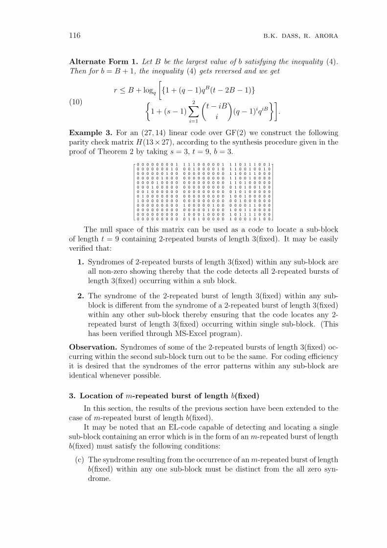
116 b.k. dass, r. arora
Alternate Form 1. Let B be the largest value of b satisfying the inequality (4).Then for b = B + 1, the inequality (4) gets reversed and we get
r ≤ B + logq
[1 + (q − 1)qB(t− 2B − 1)
1 + (s− 1)
2∑i=1
(t− iB
i
)(q − 1)iqiB
].
(10)
Example 3. For an (27, 14) linear code over GF(2) we construct the followingparity check matrix H(13×27), according to the synthesis procedure given in theproof of Theorem 2 by taking s = 3, t = 9, b = 3.
0 0 0 0 0 0 0 0 1 1 1 1 0 0 0 0 0 1 1 1 0 1 1 1 0 0 10 0 0 0 0 0 0 1 0 0 0 1 0 0 0 0 1 0 1 1 0 0 1 0 0 1 00 0 0 0 0 0 1 0 0 0 0 0 0 0 0 0 0 0 1 1 0 0 1 1 0 0 00 0 0 0 0 1 0 0 0 0 0 0 0 0 0 0 0 0 1 1 0 0 1 0 0 0 00 0 0 0 1 0 0 0 0 0 0 0 0 0 0 0 0 0 1 1 0 1 0 0 0 0 00 0 0 1 0 0 0 0 0 0 0 0 0 0 0 0 0 0 0 1 0 1 0 0 1 0 00 0 1 0 0 0 0 0 0 0 0 0 0 0 0 0 0 0 0 1 0 1 0 0 0 0 00 1 0 0 0 0 0 0 0 0 0 0 0 0 0 0 0 0 1 0 0 1 0 0 0 0 01 0 0 0 0 0 0 0 0 0 0 0 0 0 0 0 0 0 0 0 1 0 0 0 0 0 00 0 0 0 0 0 0 0 0 1 0 0 0 0 0 1 0 0 0 0 0 0 1 1 0 0 00 0 0 0 0 0 0 0 0 0 0 0 0 0 1 0 0 0 1 0 0 1 1 0 0 0 00 0 0 0 0 0 0 0 0 1 0 0 0 1 0 0 0 0 1 0 1 1 1 1 0 0 00 0 0 0 0 0 0 0 0 0 1 0 1 0 0 0 0 0 1 0 0 0 1 0 1 0 0
The null space of this matrix can be used as a code to locate a sub-blockof length t = 9 containing 2-repeated bursts of length 3(fixed). It may be easilyverified that:
1. Syndromes of 2-repeated bursts of length 3(fixed) within any sub-block areall non-zero showing thereby that the code detects all 2-repeated bursts oflength 3(fixed) occurring within a sub block.
2. The syndrome of the 2-repeated burst of length 3(fixed) within any sub-block is different from the syndrome of a 2-repeated burst of length 3(fixed)within any other sub-block thereby ensuring that the code locates any 2-repeated burst of length 3(fixed) occurring within single sub-block. (Thishas been verified through MS-Excel program).
Observation. Syndromes of some of the 2-repeated bursts of length 3(fixed) oc-curring within the second sub-block turn out to be the same. For coding efficiencyit is desired that the syndromes of the error patterns within any sub-block areidentical whenever possible.
3. Location of m-repeated burst of length b(fixed)
In this section, the results of the previous section have been extended to thecase of m-repeated burst of length b(fixed).
It may be noted that an EL-code capable of detecting and locating a singlesub-block containing an error which is in the form of an m-repeated burst of lengthb(fixed) must satisfy the following conditions:
(c) The syndrome resulting from the occurrence of an m-repeated burst of lengthb(fixed) within any one sub-block must be distinct from the all zero syn-drome.
error locating codes dealing with repeated burst errors 117
(d) The syndrome resulting from the occurrence of any m-repeated burst oflength b(fixed) within a single sub-block must be distinct from the syndromeresulting likewise from any m-repeated burst of length b(fixed) within anyother sub-block.
In this section, we shall derive two results. The first result gives a lowerbound on the number of check digits required for the existence of a linear codeover GF(q) capable of detecting and locating a single sub-block containing errorsthat are m-repeated bursts of length b(fixed). In the second result, we derive anupper bound on the number of check digits which ensures the existence of such acode.
Theorem 3. The number of parity check digits r in an (n, k) linear code subdi-vided into s sub-blocks of length t each, that locates a single corrupted sub-blockcontaining errors that are m-repeated bursts of length b(fixed) is at least
logq1 + s(qt−b+1−1) when t− b + 1 < mb
logq1 + s(qmb−1) when t− b + 1 ≥ mb.(11)
Proof. The proof of this result is on the similar lines as that of proof of Theorem 1so we omit the proof.
Remark 2. For m = 2, this result coincides with the Theorem 1 when 2-repeatedbursts of length b(fixed) are considered.
For m = 1, this result is similar to the result obtained in the Theorem 1 dueto Dass and Chand [7] when bursts of length b(fixed) are considered.
In the following result we derive another bound on the number of check digitsrequired for the existence of the code considered in the Theorem 3.
Theorem 4. A code capable of detecting an m-repeated burst of length b(fixed)within a single sub-block and of locating that sub-block can always be constructedprovided that
r > (b− 1) + logq
[ m−1∑i=0
(t− (i + 1)b + i
i
)· (q − 1)iqi(b−1)
·1+(s−1)
m∑i=1
(t−ib+i
i
)(q−1)iqi(b−1)
](12)
where r is the number of check digits.
Proof. As in Theorem 3, we omit the proof because proof of this result is on thesimilar lines as that of proof of Theorem 2.
Remark 3. For m = 2, this result coincides with Theorem 2 when 2-repeatedbursts of length b(fixed) are considered.
For m = 1, this result coincides with the result obtained in Theorem 2 dueto Dass and Chand [7] when bursts of length b(fixed) are considered.
118 b.k. dass, r. arora
References
[1] Abramson, N.M., A class of systematic codes for non-independent errors,IRE Trans. on Information Theory, IT-5(4) (1959), 150–157.
[2] Alexander, A.A., Gryb, R.M. and Nast, D.W., Capabilities of thetelephone network for data transmission, Bell System Tech J., 39 (3) (1960),431–476.
[3] Berardi, L., Dass, B.K., Verma, R., On 2-repeated burst error detec-ting codes, Journal of Statistical Theory and Practice, 3 (2) (2009), 381–391.
[4] Chien, R.T. and Tang, D.T., On definitions of a burst, IBM Journal ofResearch and Development, 9 (4) (1965), 292–293.
[5] Dass, B.K., On a burst-error correcting codes, J. Inf. Optimization Sci-ences, 1 (3) (1980), 291–295.
[6] Dass, B.K., Burst-Error locating linear codes, Journal of Information andOptimization Sciences, 3 (1) (1982), 77–80.
[7] Dass, B.K. and Chand, K., Linear codes locating correcting burst errors,DEI Journal of Science and Engineering Research, 4 (2) (1986), 41–46.
[8] Dass, B.K., Garg, P. and Zannetti, M., Some combinatorial aspectsof m-repeated burst error detecting codes, Journal of Statistical Theory andPractice, 2 (4) (2008), 707–711.
[9] Dass, B.K., Garg, P. and Zannetti, M., On Repeated Burst ErrorDetecting and Correcting Codes, In the special volume of East-West J. ofMathematics: Contributions in General Algebra II (eds. Nguyen Van Sanhand Nittiya Pabhapote), 2008, 79–98.
[10] Dass, B.K. and Garg, P., On 2-repeated burst codes, Ratio Mathematica– Journal of Applied Mathematics, 19 (2009), 11–24.
[11] Fire, P., A class of multiple-error-correcting binary codes for non-indepen-dent errors, Sylvania Report RSL-E-2, Sylvania Reconnaissance SystemsLaboratory, Mountain View, Calif., 1959.
[12] Hamming, R.W., Error-detecting and error-correcting codes, Bell SystemTech. J., 29 (1950), 147–160.
[13] Peterson, W.W. and Weldon, E.J., Jr., Error-Correcting Codes, 2ndedition, The MIT Press, Mass., 1972.
[14] Sacks, G.E., Multiple error correction by means of parity-checks, IRETrans. Inform. Theory IT, 4(December 1958), 145–147.
[15] Srinivas, K.V., Jain, R., Saurav, S. and Sikdar, S.K., Small-worldnetwork topology of hippocampal neuronal network is lost, in an in vitroglutamate injury model of epilepsy, European Journal of Neuroscience, 25(11) (2007), 3276–3286.
[16] Wolf, J. and Elspas, B., Error-locating codes A new concept in errorcontrol, IEEE Transactions on Information Theory, 9 (2) (1963), 113–117.
Accepted: 06.02.2010
italian journal of pure and applied mathematics – n. 29−2012 (119−134) 119
M-INJECTIVITY IN THE CATEGORY Act-S
Leila Shahbaz
Department of MathematicsUniversity of MaraghehMaragheh 55181-83111Irane-mail: [email protected]
Abstract. Injectivity is one of the central notions in many branches of mathematics.Different kinds of injectivity with respect to the class of all monomorphisms and withrespect to some special subclasses of monomorphisms in the category Act-S of acts overa semigroup S have been studied before. In this paper, we take the category Act-S ofacts over a semigroup S, and M as an arbitrary subclass of monomorphisms, and studysome kinds of injectivity with respect to M. Also, the behaviour of these notions ofinjectivity with respect to products, coproducts, and direct sums is studied. As a resultwe give some characterizations of semigroups.
Keywords: M-injective, weakly M-injective, ideal M-injective.
2000 Mathematics Subject Classification: 08A60, 18A20, 20M30, 20M50.
1. Introduction and preliminaries
One of the very useful notions in many branches of mathematics as well as incomputer science is the notion of acts of a semigroup or a monoid on a set. Inthe following we first recall some facts about the category Act-S needed in thispaper.
Let S be a semigroup, A be a set, and
µ : A× S −→ A(a, s) 7−→ as := µ(a, s),
be a map. The set A is called a (right) S-act or a (right) act over S, if the mapµ satisfies a(st) = (as)t for a ∈ A and s, t ∈ S. In this case, µ is called the actionof S on A.
If S is a monoid with 1 as its identity, we usually also require that a1 = a fora ∈ A.
A subset A′ of an S-act A is said to be a subact of A if a′s ∈ A′ for all s ∈ Sand a′ ∈ A′; and in this case we write A′ ≤ A.
120 leila shahbaz
A homomorphism (also called an equivariant map or an S-map) from an S-act A to an S-act B is a function from A to B such that for each a ∈ A, s ∈ S,f(as) = f(a)s.
Since idA and the composition of two S-maps are S-maps, we have the cate-gory Act-S of all right S-acts and S-maps between them.
Note that, the class of S-acts is an equational class, and so the category Act-Sis complete and cocomplete (has all products, equalizers, pullbacks, coproducts,coequalizers, and pushouts). In fact, limits and colimits in this category are com-puted as in the category Set of sets and equipped with a natural action. Also,monomorphisms (epimorphisms) in Act-S are exactly one-one (onto) S-maps.Therefore, we do not distinguish between monomorphisms of acts and inclusions,and call an S-act B containing (an isomorphic copy of) an S-act A an extensionof A.
An element z of S is called a right zero element if for each s ∈ S, sz = z.Also, an element z of S is called a left zero element if for each s ∈ S, zs = z. Anelement 0 or θ of S is a zero element if it is right and left zero.
An S-act A is said to be finitely generated if A =n⋃
i=1
aiS1, for some a1, ...,
an ∈ A and n ∈ N , where S1 is the semigroup S with an adjoined identity 1. Wesay that a semigroup S is finitely generated if it is finitely generated as an S-actwith its operation as the action.
A semigroup S is said to be Noetherian if it satisfies the ascending chaincondition on its right ideals.
A semigroup S is said to be left reversible if every two right ideals of S have anonempty intersection. For more information about semigroups and acts see [6],[8] and [9].
An S-act A is said to be decomposable if there exist subacts B, C ⊆ A suchthat A = B ∪ C and B ∩ C = ∅. Otherwise, A is called indecomposable.
An act A is called torsion free if for any x, y ∈ A and for any element s ∈ Sthe equality xs = ys implies x = y.
Recall that for a category A and a subclass M of monomorphisms in A, wesay that A satisfies the M-transferability property if any diagram
Af //
g
²²
B
C
with f ∈M can be completed to a commutative diagram
Af //
g
²²
B
u
²²C
v // D
with v ∈M.
M-injectivity in the category Act-S 121
Note that, since pushouts exist in the category Act-S, the above conditionis equivalent to “pushout transfer monomorphism”; that is, the pushout mapcorresponding to a morphism in M again belongs to M.
Recall that for a family Ai : i ∈ I of S-acts with a unique fixed element 0,
the direct sum⊕i∈I
Ai is defined to be the subact of the product∏i∈I
Ai consisting
of all (ai)i∈I such that ai = 0 for all i ∈ I except a finite number.
2. M-injectivity and some kinds of weak M-injectivity
In this section, we study M-injectivity and some kinds of weak M-injectivity ofacts for a subclass M of monomorphisms. Any map with prefix M means beingin M.
Definition 2.1 We call an S-act E:
(1) M-injective if it is injective with respect to M-morphisms. An injective actwith respect to all act monomorphisms is simply called injective.
(2) M-absolute retract if it is a retract of each of its M-extensions; that is forevery M-morphism h : A → B there exists an S-map g : B → A such thatgh = idA.
Clearly, if A is an injective S-act, then it is M-injective for any subclass Mof monomorphisms, but the converse is not necessarily true. For example, takeM as the class of sequentially dense or sequentially pure monomorphisms and see[10] and [2].
The following theorem is one of the important theorems about injectivity ofS-acts with respect to any subclass of monomorphisms. This theorem was firstproved by P. Berthiaume in [4] for injective acts. H. Barzegar [3] and B. Ba-naschewski [1] proved it for M-injective acts for any subclass M of monomor-phisms.
Theorem 2.2 Let S be a semigroup. Then, if pushouts transfer M-morphisms,the following are equivalent for an S-act A:
(i) A is M-injective.
(ii) A is an M-absolute retract.
Here we give a criterion like the Skornjakov-Baer criterion [13], for M-injectivityof acts over a semigroup.
Theorem 2.3 Let for each M-extension A of B, D be an M-extension of B withD ⊆ A. Then, for an S-act E, the following are equivalent:
(i) E is M-injective.

122 leila shahbaz
(ii) For every M-morphism h : B ½ B ∪ aS1 to a singly generated extensionof B and every S-map f : B → E there exists an S-map g : B ∪ aS1 → Esuch that gh = f .
Proof. It is clear that (i)⇒(ii).
(ii)⇒(i) Let h : B ½ A be an M-morphism and f : B → E be an S-map. Applying Zorn’s Lemma on the poset of all subacts (Dα, gα) of A whichare M-extensions of B, with h(B) ⊆ Dα and such that there exists an S-mapgα : Dα → E with gαh = f with the order
(Dα, gα) ≤ (Dβ, gβ) ⇔ Dα ⊆ Dβ, gβ |Dα= gα
we get a maximal such subact, say (D, g). If D = A then the proof is complete.Otherwise, there exists a ∈ A − D. Now, since by the hypothesis D ∪ aS1 is anM-extension of B we get that g : B → D ∪ aS1 is an M-morphism, and by (ii)there is an S-map g which extends g. This contradicts the maximality of D, soA = D.
Now, we define some kinds of weak M-injectivity and then compare themwith M-injectivity.
Definition 2.4 A right ideal I of S is called a right M-ideal if the inclusion mapfrom I into S belongs to M.
Definition 2.5 An S-act A is said to be
(1) ideal M-injective, if every S-map f : I → A from a right M-ideal I of Scan be represented as λa, for some a ∈ A.
(2) weakly M-injective if for each right M-ideal I of S, any S-map f : I → Acan be extended to an S-map g : S → A.
(3) finitely M-injective (cM-injective) if for eachM-morphism h : F → B froma finitely generated (cyclic) act F and for any S-map f : F → A there exitsan S-map g : B → A such that gh = f .
(4) FM-injective (PM-injective) if every S-map f : I → A from a finitelygenerated (principal) right M-ideal I of S can be extended to an S-mapf : S → A.
(5) A semigroup S is called completely M-injective if all right S-acts are M-injective. Similarly for the other types of M-injectivity.
Remark 2.6
(1) Ideal (weakly) M-injective acts need not be M-injective in the usual sense(let M = Mono and see [9]).

M-injectivity in the category Act-S 123
(2) Ideal M-injectivity implies weak M-injectivity but weakly M-injective actsneed not be ideal M-injective. For the case where S is a monoid, ideal M-injectivity coincides with weak M-injectivity.
Lemma 2.7 A retract of any kind of M-injective act is M-injective of that type.
The following results show when all acts are finitely M-injective.
Lemma 2.8 If pushouts transferM-morphisms then every finitely generated finitelyM-injective S-act is M-injective.
Proof. Let A be a finitely generated finitely M-injective S-act. Consider thefollowing diagram
Ai //
idA
²²
B
A
in which B is an M-extension of A. Using that A is finitely generated, thereexists π : B → A such that π i = idA. This implies that A is an M-absoluteretract. Now, by Theorem 2.2, A is M-injective.
Theorem 2.9 If pushouts transfer M-morphisms then a semigroup S is com-pletely finitely M-injective if and only if all finitely generated S-acts are M-injective.
Proof. (⇒) The proof is similar to the proof of the above lemma.
(⇐) Let A be any S-act and h : F → B be an M-morphism from a finitelygenerated act F , and f : F → A be any S-map. Then, by hypothesis, F isM-injective and so an M-absolute retract, by Theorem 2.2. Thus there exists anS-map g : B → F such that gh = idF . Then the composite fg : B → A is anS-map with (fg)h = f . So, A is finitely M-injective.
Proposition 2.10 An S-act A with a zero element is cM-injective if and onlyif for any M-morphism h : P ½ D from a cyclic act P into any indecomposableact D, any S-map f : P → A can be extended to an S-map g : D → A.
Proof. (⇒) is clear.
(⇐) Let A be an S-act with a zero element and h : P → B be an M-morphism from a cyclic act P, and f : P → A be any S-map. Consider the
decomposition of B =⊔i∈I
Bi into its indecomposable subacts Bi which exists by
Theorem I.5.10 of [9]. Since P is cyclic, there exists i ∈ I such that h(P ) ⊆ Bi.Thus by the hypothesis there exists an S-map g : Bi → A which extends f . Define
f : B =⊔i∈I
Bi → A by
f(b) =
g(b) if b ∈ Bi
θ if b 6∈ Bi
where θ is the zero element of A. Then f is an S-map which extends f .

124 leila shahbaz
The following results show when all acts are cM-injective.
Lemma 2.11 If pushouts transfer M-morphisms then every cyclic cM-injectiveS-act is M-injective.
Proof. It is similar to the proof of Theorem 2.9 by replacing finitely generatedacts with cyclic acts.
Theorem 2.12 If pushouts transfer M-morphisms then a semigroup S is com-pletely cM-injective if and only if all cyclic S-acts are M-injective.
Proof. The proof is similar to the proof of the above lemma.
The following theorem characterizes semigroups over which all acts are idealM-injective.
Theorem 2.13 Every S-act is ideal M-injective if and only if every right M-ideal of the semigroup S is generated by an idempotent.
Proof. Consider the identity map idI from a right M-ideal I of S which is ofthe form λa for some element a in I, by hypothesis. Thus, a = idI(a) = λa(a) =aa = a2 and so a is an idempotent element. For the converse, let I = eS bea right M-ideal of S, where e is an idempotent element. Consider an S-mapf : I = eS → A. Thus f = λa for a = f(e). Thus A is ideal M-injective.
In the following we characterize semigroups over which all acts are weaklyM-injective.
Theorem 2.14 The following conditions are equivalent:
(1) Each right M-ideal of S is a retract of S.
(2) S is completely weakly M-injective.
(3) Each right M-ideal of S is weakly M-injective.
Proof. (1) ⇒ (2) Let A be an S-act, and f : I → A be an S-map from aright M-ideal I of S. By the hypothesis, there is a retraction g : S → I. Thenfg : S → A is an S-map which extends f . So, A is weakly M-injective.
(2) ⇒ (3) is clear.
(3) ⇒ (1) Let I be a right M-ideal of S. Then there exists an S-map π fromI to S with π |I= idI , since I is weakly M-injective by (2). So I is a retract of S.
In the following we characterize semigroups over which all acts are FM-injective (PM-injective).
Theorem 2.15 The following conditions are equivalent:
M-injectivity in the category Act-S 125
(1) Each finitely generated (principal) right M-ideal of S is a retract of S.
(2) S is completely FM-injective (PM-injective).
(3) Each finitely generated (principal) rightM-ideal of S is FM-injective (PM-injective).
Proof. (1) ⇒ (2) Let A be an S-act, and f : I → A be an S-map from afinitely generated (principal) right M-ideal I of S. By the hypothesis, there is aretraction g : S → I. Then fg : S → A is an S-map which extends f . So, A isFM-injective (PM-injective).
(2) ⇒ (3) is clear.
(3) ⇒ (1) Let I be a finitely generated (principal) right M-ideal of S. Thenthere exists an S-map π from I to S with π |I= idI , since I is FM-injective(PM-injective) by (2). So I is a retract of S.
Definition 2.16 A right M-ideal I of S is called M-intersection large in S if theintersection of I with any nonempty right M-ideal of S is always nonempty.
Theorem 2.17 Suppose that S is a semigroup with a zero element and for eachright M-ideal I of S, J is a right M-ideal of S with I ⊆ J . Then a right S-act Ais weakly M-injective if and only if for any M-intersection large right M-ideal Iof S, every S-map from I into A can be extended to an S-map from S into A.
Proof. The only if part is obvious. To prove the converse, let I be any rightM-ideal of S and f be an S-map from I into A. Let P be the set of pairs (J, g)where J is a right M-ideal of S which contains I and g is an S-map from J intoA which extends f . Consider P as the ordered set with the order
(J1, g1) ≤ (J2, g2) ⇔ J1 ⊆ J2, g2 |J1= g1.
Applying Zorn’s lemma, P has a maximal element (K, gK). If K is not an M-in-tersection large ideal, there exists a rightM-ideal L 6= ∅ of S such that L ∩K = ∅.Define a mapping g∗ : K ∪ L → A by
g∗(s) =
gK(s) if s ∈ K
θ (the zero element of A) if s ∈ L
It is easy to see that g∗ is an S-map from K ∪ L into A, which extends gK andhence f . Thus (K∪L, g∗) ∈ P , which contradicts the fact that (K, gK) is maximalin P . Hence K must be an M-intersection large ideal. Hence by the hypothesis,gK can be extended to an S-map from S into A, which is therefore an extensionof f .
Definition 2.18 A semigroup S is called M-Noetherian if it satisfies the ascen-ding chain condition on its right M-ideals.
126 leila shahbaz
Remark 2.19 If a semigroup S is M-Noetherian then every right M-ideal I ofS is finitely generated. For if, let I be a right M-ideal of S, and assume thatI 6= ∅ is not finitely generated. Thus there exists x1 ∈ I. Let x1, x2, x3, . . . ⊆ Ibe a countable subset of generating elements of I which are different. Thus
〈x1〉 = I1 ⊆ 〈x1, x2〉 = I2 ⊆ 〈x1, x2, x3〉 = I3 ⊆ ... ⊆ 〈x1, x2, ..., xn〉 = In ⊆ ...
is an ascending chain of right M-ideals of S which does not stop and this is acontradiction. Thus I is finitely generated.
Theorem 2.20 Let S be a left reversible and right M-Noetherian semigroup.Suppose A is a torsion free S-act such that every cyclic subact of A is ideal M-injective. Then A is itself ideal M-injective.
Proof. Let I =n⋃
i=1
siS1 be a right M-ideal of S, and f : I → A be an S-map. If
f(si) = xi, then f |siS1 : siS1 → xiS
1 is an S-map. Since xiS1 is ideal M-injective
by the assumption, there exists ai ∈ xiS1 such that f(si) = aisi, i = 1, 2, . . . , n.
Since by left reversiblity of S the intersection of all right ideals of S are nonempty,there exists ci ∈ S such that s1c1 = s2c2 = . . . = sncn. Then f(s1)c1 = f(s2)c2 =. . . = f(sn)cn and so a1s1c1 = a2s2c2 = . . . = ansncn. Since A is torsion freewe have a1 = a2 = . . . = an = a. Thus f(s) = as, s ∈ I and hence A is idealM-injective.
Remark 2.21 The condition that S is left reversible is necessary in the abovetheorem. For, takeM as the class of all monomorphisms and see [11], Example 1.3.
Theorem 2.22 Let S be an M-Noetherian semigroup, A be an S-act which isnot finitely generated and each proper subact of A is ideal M-injective. Then Ais ideal M-injective.
Proof. Let I =n⋃
i=1
siS1 be a right M-ideal of S, and f : I → A be an S-map. If
f(I) = A, then A =n⋃
i=1
aiS1 where f(si) = ai ∈ A, which implies that A is finitely
generated. Hence f(I) 6= A. Then f(I) is ideal M-injective by the hypothesisand so f : I → f(I) is given by f(s) = as for every s ∈ I. Hence A is idealM-injective.
Remark 2.23 The condition that A is not finitely generated is necessary in theabove theorem. For, take M as the class of all monomorphisms and see [11],Example 1.5.
M-injectivity in the category Act-S 127
3. Products, coproducts, and direct sums of different kindsof M-injective acts
In this section we consider the behaviour of different kinds of M-injective actswith respect to products, coproducts, and direct sums.
In the following theorems, it is shown that as usual, the above types of M-injectivity well-behaves with respect to products similar to the case of injectivityusing the universal property of products, but not as well with coproducts anddirect sums.
Theorem 3.24 Let Ai : i ∈ I be a family of S-acts. Then the product∏i∈I
Ai is
M-injective (finitely M-injective, cM-injective, FM-injective, PM-injective) ifeach Ai is M-injective (finitely M-injective, cM-injective, FM-injective, PM-injective). The converse is true if each Ai has a zero element.
In the case of weakly M-injective (ideal M-injective) acts we have the fol-lowing.
Theorem 3.25 Let Ai : i ∈ I be a family of S-acts. Then the product∏i∈I
Ai is
weaklyM-injective (idealM-injective) if and only if each Ai is weaklyM-injective(ideal M-injective).
Proof. The fact that the product of weakly M-injective acts is weakly M-injective is proved similar to the case of injectivity using the universal property
of products. To prove the converse, let A =∏i∈I
Ai be weakly M-injective, k ∈ I,
and define an S-map fi : J → Ai by fk = f , and for i 6= k, f = λai, where ai
is any element of Ai and J is an M-right ideal of S. Then we get an S-map f
using the universal property of products which extends to an S-map f : S → A
by weak M-injectivity of A. Now, pkf : S → Ak extends f , where pk : A → Ak isthe kth projection map. So A is weakly M-injective.
In regard with coproducts, first note that the following is trivially true.
Proposition 3.26 Let Ai : i ∈ I be a family of S-acts with a zero element.
If the coproduct∐i∈I
Ai is M-injective (ideal M-injective, weakly M-injective,
finitely M-injective, cM-injective, FM-injective, PM-injective) then each Ai
is M-injective (ideal M-injective, weakly M-injective, finitely M-injective, cM-injective, FM-injective, PM-injective).
The converse of the above theorem is not necessarily true in general (see [10],Theorem 3.4). But in the case of cM-injective (PM-injective) acts the converseis also true.

128 leila shahbaz
Proposition 3.27 Let Ai : i ∈ I be a family of cM-injective (PM-injective)
S-acts. Then the coproduct∐i∈I
Ai is cM-injective (PM-injective).
Proof. Let Ai : i ∈ I be a family of cM-injective acts. Notice that for any
M-morphism g : F → B from a cyclic act F and any S-map f : F →∐
Ai we
have Imf ⊆ Ai for some i ∈ I. Hence f can be extended to an S-map f , sinceAi is cM-injective.
In the case of ideal M-injective (weakly M-injective) acts we have the fol-lowing.
Theorem 3.28 Let a semigroup S be left reversible. Then the coproduct∐i∈I
Ai
of each family of ideal M-injective (weakly M-injective) acts is ideal M-injective(weakly M-injective).
Proof. Let Ai : i ∈ I be a family of ideal M-injective acts. Let f : J →∐i∈I
Ai,
which J is an M-right ideal of S, be an S-map. Suppose there exist i, j ∈ I, i 6= j,with Imf ∩Ai 6= ∅ and Imf ∩Aj 6= ∅. Then J is a disjoint union of two ideals incontradiction with left reversibility of S. This implies the existence of i ∈ I suchthat Imf ⊆ Ai. Since Ai is ideal M-injective, f can be written in the form of λa
for some a in Ai. Thus∐i∈I
Ai is ideal M-injective.
Theorem 3.29 If the coproduct∐i∈I
Ai of each family of ideal M-injective acts is
ideal M-injective then any two right M-ideals of S have a nonempty intersection.
Proof. Let I, J be two M-right ideals of S such that I ∩ J = ∅. By assumptionΘtΘ = b1, b2, where Θ is the one element act, is ideal M-injective. The S-mapf : I t J → Θ tΘ given by
f(s) =
b1 if s ∈ I
b2 if s ∈ J
can not be written in the form of λa for some a ∈ ΘtΘ which is a contradiction.Thus each pair of M-right ideals of S have a nonempty intersection.
For the direct sum of different kinds of M-injectivity we first trivially have:
Theorem 3.30 Let Ai : i ∈ I be a family of S-acts with zero such that the
direct sum⊕i∈I
Ai is M-injective (ideal M-injective, weakly M-injective, finitely
M-injective, cM-injective, FM-injective, PM-injective). Then each Ai is M-injective (idealM-injective, weaklyM-injective, finitelyM-injective, cM-injective,FM-injective, PM-injective).
M-injectivity in the category Act-S 129
Remark 3.31 The converse of the above theorem is true in the case of finitelyM-injective, cM-injective, FM-injective, and PM-injective acts. But it is not truein general, for example take M as the class of sequentially dense monomorphismsand see [10].
Proposition 3.32 Each direct sum of finitely M-injective (cM-injective, FM-injective, PM-injective) acts is finitely M-injective (cM-injective, FM-injective,PM-injective).
Proof. Let Aii∈I be a family of finitely M-injective acts. Consider the diagram
Xλ //
f ²²
Y
⊕i∈I
Ai
in which λ is anM-morphism, f is a homomorphism, and X is a finitely generatedact. Let x1, x2, ..., xn be the generating set of X. Then for each j, the element
f(xj) in⊕i∈I
Ai has only finitely many nonzero coordinates. Since there are only
finitely many xj, the set f(x1), f(x2), ..., f(xn) collectively involves only finitelymany Ai, say Ai1 , ..., Ain . Hence Imf ⊆ Ai1
⊕...
⊕Ain which, being a finite
direct sum of finitely M-injective acts (which is in fact a product of finitelyM-injective acts), is finitely M-injective, by Theorem 3.25. Hence there is ahomomorphism f : Y → Ai1
⊕...
⊕Ain which extends f . We may regard f as a
homomorphism whose image is in the larger S-act⊕i∈I
Ai.
Theorem 3.33 Let a semigroup S be (M-)Noetherian. Then the direct sum⊕i∈I
Ai of each family of weakly M-injective acts is weakly M-injective.
Proof. The proof is similar to the proof of the above theorem by replacing Xwith every right M-ideal I of S.
About direct sum of ideal M-injective acts we have
Theorem 3.34 Let S be a semigroup with the zero 0 and for each family
Ii : i ∈ I of right M-ideals of S, I =⋃i∈I
Ii be a right M-ideal of S. Then
each direct sum of (ideal M-) injective acts is ideal M-injective if and only if Sis M-Noetherian.
Proof. (⇒) Let 0 = I0 ⊆ I1 ⊆ . . . ⊆ Ii ⊆ . . . be an ascending chain of rightM-ideals of S, and I =
⋃i∈I Ii. By the hypothesis, I is a right M-ideal of S.
Consider the Rees factor acts I/Ii for each i, and let Ei be the injective hull of
130 leila shahbaz
I/Ii. Then E =⊕
i
Ei is ideal M-injective by the hypothesis. Consider natural
epimorphisms fi : I → I/Ii and define an S-map f : I → E by f(s) = (fi(s))i.Notice that for each s ∈ I only finitely many components of f(s) are nonzero,because s ∈ Ik for some k, and so fi(s) = 0 for all i ≥ k. Now, since E isideal M-injective by assumption, there exists an element a ∈ E, f = λa. Since
a ∈ E =⊕
i
Ei, a = (a1, a2, . . . , ak, . . .), so there is t such that ak = 0 for all
k ≥ t. Then since for any x ∈ I, f(x) = ax, and since (ax)t = atx = 0, it followsthat I ⊆ It. Hence It+1 = It+2 = . . . = I. Thus S satisfies the ascending chaincondition on its M-right ideals and so is M-Noetherian.
(⇐) Let Ai : i ∈ I be a family of ideal M-injective acts with zero elements.
Let f : I →⊕i∈I
Ai be an S-map from a right M-ideal I of S and assume that I is
generated by s1, s2, . . . , sn, since S is M-Noetherian. Then, since only finitelymany components of each f(si) are nonzero, we get that Imf is contained in adirect sum of finitely many Ai, say i1, i2, . . . , im. Then, Ai1⊕Ai2⊕· · ·⊕Aim which isin fact a product, is idealM-injective, f = λa, for some a ∈ Ai1⊕Ai2⊕· · ·⊕Aim ⊆⊕i∈I
Ai.
Proposition 3.35 Let for each family Ii : i ∈ I of right M-ideals of a semi-
group S, I =⋃i∈I
Ii be a right M-ideal of S. If every finitely M-injective act is
ideal M-injective then S is M-Noetherian. The converse is true if S is a monoid.
Proof. Let Ai : i ∈ I be a family of idealM-injective acts. Since each idealM-injective act is finitely M-injective thus each Ai is finitely M-injective. We knowthat each direct sum of finitely M-injective acts is finitely M-injective and so bythe hypothesis it is ideal M-injective. So, by Theorem 3.34, S is M-Noetherian.
For the converse, let S be a monoid, A be a finitely M-injective act, andf : I → A be an S-map from a right M-ideal I of S. Since S is M-Noetherian, Iis finitely generated. Now, since A is finitely M-injective there exists an S-mapg : S → A which extends f . Then g is of the form λa for a = g(1) where 1 is theidentity element of the monoid S. Thus f is also of the form λa and hence A isideal M-injective.
We recall the following Theorem from [12].
Theorem 3.36 Each direct sum of injective S-acts is injective if and only if Sis Noetherian.
Corollary 3.37 If S is an M-Noetherian semigroup and ideal M-injectivity(weak M-injectivity) for S-acts implies injectivity, then S must be Noetherian.
Proof. By Theorem 3.36, S is Noetherian if and only if every direct sum ofinjective S-acts is injective. Now, if Ai : i ∈ I is any family of injective acts
M-injectivity in the category Act-S 131
then they are also ideal M-injective, and so, by Theorem 3.34, their direct sumis ideal M-injective and hence injective by the hypothesis, and so the result.
Definition 3.38 An S-act A is called countably∑
-idealM-injective if any count-able direct sum of A with itself is ideal M-injective.
Theorem 3.39 Let for each family Ii : i ∈ I of right M-ideals of S, I =⋃i∈I
Ii
be a right M-ideal of S. Then the following are equivalent:
(1) Each direct sum of injective acts is ideal M-injective.
(2) Each injective act is countably∑
-ideal M-injective.
(3) S is M-Noetherian.
Proof. (1)⇒(2) is clear.
(2)⇒(3) Applying the notations of Theorem 3.34, put A =∏n∈IN
En. Then
A is injective, and so by (2),⊕n∈IN
A is ideal M-injective. But, A =∏n∈IN
En
= Em ⊕∏
n6=m
En, for each m ∈ IN. Thus⊕m∈IN
A =⊕m∈IN
Em ⊕⊕m∈IN
∏
n 6=m
En =
E⊕⊕m∈IN
∏
n 6=m
En, which means that E is a direct summand of an ideal M-injective
act and hence is ideal M-injective, by Theorem 3.30. The rest of the proof issimilar to Theorem 3.34.
(3)⇒(1) is proved similar to Theorem 3.34.
4. Some Baer conditions
The condition that weak injectivity implies injectivity is known as the Baer Cri-terion for injectivity. In this section we give some Baer conditions.
Definition 4.40 An S-act A is called
(i) quasi injective if any S-map f : B → A from a subact B of A can beextended to A.
(ii)∑
-injective (∑
-quasi injective) if every direct sum of A with itself is injective(quasi injective).
Theorem 4.41 The following conditions are equivalent:
(1) Each weakly M-injective act is injective and S is M-Noetherian.
(2) Each FM-injective act is injective.
132 leila shahbaz
(3) Each FM-injective act is quasi injective with a zero element.
Proof. (1)⇒(2) Since S is M-Noetherian, each right M-ideal is finitely genera-ted, so an act A is weakly M-injective if and only if it is FM-injective.
(2)⇒(3) is clear.
(3)⇒(2) Let A be FM-injective and E(A) be the injective hull of A. Then,by Theorem 3.32, A ⊕ E(A) is FM-injective and hence by (3) quasi injective.The rest of the proof is quite similar to the proof of (4)⇒(1) of Theorem 4.42.
(2)⇒(1) Since every weakly M-injective act is FM-injective, we get the firstpart. To see that S is M-Noetherian, using Theorem 3.36 we show that anydirect sum of injective acts is injective. This is true because of (2) and since ,byProposition 3.32, any direct sum of FM-injective acts is FM-injective.
Theorem 4.42 If S is an M-Noetherian semigroup, then the following are equi-valent:
(1) Each weakly (ideal) M-injective act is injective.
(2) Each weakly (ideal) M-injective act is∑
-injective and has a fixed element.
(3) Each weakly (ideal) M-injective act is∑
-quasi injective and has a fixedelement.
(4) Each weakly (ideal) M-injective act is quasi injective and has a fixed ele-ment.
Proof. (1)⇒(2) is true using Theorem 3.33. Also recall that each injective acthas a fixed element.
(2)⇒(3) and (3)⇒(4) are clear.
(4)⇒(1) Let A be weakly M-injective and E(A) be the injective hull of A.Then A ⊕ E(A) is weakly M-injective and hence quasi injective by (4). So,
considering the monomorphism A → E(A)τE(A)−→ A ⊕ E(A), where τE(A) is the
injection x 7→ (0, x), and the S-map τA : A → A ⊕ E(A), there exists an S-map g : A ⊕ E(A) → A ⊕ E(A) such that gτE(A) |A= τA. This implies thatpAgτE(A) |A= idA and so A is a retract of the injective act E(A) and hence isinjective.
Theorem 4.43 Let for each family Ii : i ∈ I of right M-ideals of S, I =⋃i∈I
Ii
be a right M-ideal of S. Then the following are equivalent:
(1) The direct sum of each family of weaklyM-injective acts is idealM-injective.
(2) S is M-Noetherian and weak M-injectivity implies ideal M-injectivity.
(3) Each FM-injective act is ideal M-injective.

M-injectivity in the category Act-S 133
Proof. (1)⇒(2) Similar to the proof of Theorem 3.34 it is shown that S is M-Noetherian, the rest is clear.
(2)⇒(1) It is concluded from Theorem 3.34.
(2) ⇒ (3) Since S is M-Noetherian, each right M-ideal of S is finitely gene-rated and so weak M-injectivity coincides with FM-injectivity. So (3) holds.
(3) ⇒ (2) Since every weakly M-injective act is FM-injective we get the firstpart. For the second part, let Ai : i ∈ I be a family of injective acts. Sinceeach injective act is FM-injective and since each direct sum of FM-injectiveacts is FM-injective, thus the direct sum
⊕i∈I Ai is FM-injective and so ideal
M-injective by the hypothesis. Thus S is M-Noetherian, by Theorem 3.34.
Acknowledgments. The author would like to thank Professor M. Mehdi Ebrahimiand Professor Mojgan Mahmoudi for their very useful comments and helpful con-versations during this research.
References
[1] Banaschewski, B., Injectivity and essential extensions in equationalclasses of algebras, Queen’s Papers in Pure and Applied Mathematics, 25(1970), 131-147.
[2] Barzegar, H. and Ebrahimi, M.M, Essentiality and injectivity relativeto sequential purity of acts, Semigroup Forum, 79 (2009), 128 144.
[3] Barzegar, H., Ebrahimi, M. M., Mahmoudi, M., Essentiality and in-jectivity, Appl. Categor. Struct., 18 (2010), 73-83.
[4] Berthiaume, P., The injective envelope of S-sets, Canad. Math. Bull. 10(2) (1967), 261-273.
[5] Ebrahimi, M.M., Algebra in a Grothendieck topos: injectivity in quasi-equational classes, J. Pure Appl. Algebra, 26 (3) (1982), 269-280.
[6] Ebrahimi, M.M. and Mahmoudi, M., The category of M-sets, Ital. J.Pure Appl. Math., 9 (2001), 123-132.
[7] Herrlich H. and Ehrig, H., The construct PRO of projection spaces: itsinternal structure, Lecture Notes in Computer Science, 393 (1988), 286-293.
[8] Howie, J.M., Fundamentals of Semigroup Theory, Oxford Science Publica-tions, Oxford, 1995.
[9] Kilp, M., Knauer U., and Mikhalev, A., Monoids, Acts and Categories,Walter de Gruyter, Berlin, New York, 2000.
134 leila shahbaz
[10] Mahmoudi M. and Shahbaz, L., Characterizing semigroups by sequentiallydense injective acts, Semigroup Forum, 75 (1) (2007), 116-128.
[11] Satyanarayana, M., Quasi and weakly injective S-systems, Mathema-tische Nachrichten, 71 (1) (1973), 183-190.
[12] L.A. Skornjakov, L.A., Axiomatizability of the class of injective M-sets,Trudy Seminara im. I.G. Petrovskogo, 4 (1978), 233-239 (in Russian).
[13] Skornjakov, L.A., On homological classification of monoids, Sib. Math.J., 10 (1969), 1139-1143 (in Russian). Correction ibid., 12 (1971), 689.
Accepted: 12.03.2010

italian journal of pure and applied mathematics – n. 29−2012 (135−148) 135
ON KOTHE-TOEPLITZ DUALS OF SOME NEWAND GENERALIZED DIFFERENCE SEQUENCE SPACES
A.A. Ansari
V.K. Chaudhry
Department of Mathematics and StatisticsD.D.U. Gorakhpur UniversityGorakhpur-273009Indiae-mail: [email protected] vkc [email protected]
Abstract. In this paper we define the sequence spaces 4mv,r(l∞), 4m
v,r(c) and 4mv,r(c0),
(m ∈ N, r ∈ R), and have studied some of their topological properties and have com-puted their Kothe-Toeplitz duals.
Keywords: difference sequences, α, β and γ-duals.2000 AMS Subject Classification: 40C05, 46A45.
1. Introduction
Let l∞, c and c0 be the linear spaces of bounded convergent and null sequencesx = (xk) with complex terms, respectively, normed by
‖x‖∞ = supk|xk|
where k ∈ N = 1, 2, 3, ..., the set of positive integers.In 1981, Kizmaz [8] introduced the concept of difference sequences and have
defined 4−bounded, 4− convergent and 4− null sequence spaces. Using theconcept of difference sequences, Et [4] has defined 42−bounded, 42− convergentand 42−null sequence spaces. Further, this notion was generalized by Et andColak [6] and have defined4m−bounded,4m−convergent and4m−null sequencespaces. Later on, Et and Esi [5] have defined 4m
v −bounded, 4mv −convergent
and 4mv −null sequence spaces where v = (vk) be any fixed sequence of non-zero
complex numbers. Recently, Bektas and Colak [1] have defined the sequencespaces
136 a.a. ansari, v.k. chaudhry
l∞(4mr ) = x = (xk) : (kr4m xk) ∈ l∞,
c(4mr ) = x = (xk) : (kr4m xk) ∈ c,
c0(4mr ) = x = (xk) : (kr4m xk) ∈ c0.
where m ∈ N , r ∈ R, 4mr x = (4m
r xk) = (kr4mxk) = (kr(4m−1xk −4m−1xk+1))and
4mxk =m∑
j=1
(−1)j
(mj
)xk+j.
These are Banach spaces with norm
||x||4r =m∑
i=1
|xi|+ supk
kr|4mxk|.
It is trivial that c0(4mr ) ⊂ c0(4m+1
r ), c(4mr ) ⊂ c(4m+1
r ), l∞(4mr ) ⊂ l∞(4m+1
r )and c0(4m
r ) ⊂ c(4mr ) ⊂ l∞(4m
r ) are satisfied and are strict [1].For convenience, we denote these spaces 4m
r (l∞) = l∞(4mr ), 4m
r (c) = c(4mr )
and 4mr (c0) = c0(4m
r ).Let v = (vk) be any fixed sequence of non-zero complex numbers. Now, we
define
4mv,r(l∞) = x = (xk) : (kr4m
v xk) ∈ l∞,4m
v,r(c) = x = (xk) : (kr4mv xk) ∈ c,
4mv,r(c0) = x = (xk) : (kr4m
v xk) ∈ c0.where m ∈ N , r ∈ R, 4m
v,r(x) = (kr4mv xk) = (kr(4m−1
v xk −4m−1v xk+1)) and
4mv xk =
m∑j=1
(−1)j
(mj
)vk+j xk+j.
Throughout the paper, we write X for l∞ or c or c0. 4mv,r(X) is the genera-
lization of several known sequence spaces, for instance, the following classes arisefrom 4m
v,r(X) as the special cases.
(i) If we take v = (vk) = (1, 1, ...), then 4mv,r(X) = 4m
r (X) [1].
(ii) If we take r = 0, then 4mv,r(X) = 4m
v (X) [5].
(iii) If we take v = (vk) = (1, 1, ...) and r = 0, then 4mv,r(X) = 4m(X) [6].
(iv) If we take v = (vk) = (1, 1, ...) , r = 0 and m = 2, then4mv,r(X) =42(X) [4].
(v) If we take v = (vk) = (1, 1, ...) , r = 0 and m = 1, then 4mv,r(X) = 4(X) [8].
(vi) If we take r = 0 and m = 1, then 4mv,r(X) = 4v(X) [2].

on kothe-toeplitz duals ... 137
(vii) If we take vk = 1 for all k ∈ N, r < 1 and m = 1, then 4mv,r(X) =
4r(X) [10].
2. Main results
Theorem 2.1. The sequence spaces 4mv,r(l∞), 4m
v,r(c) and 4mv,r(c0) are Banach
spaces normed by
(2.1) ||x||4v,r =m∑
i=1
|vixi|+ supk
kr|4mv xk|
Let us define the operator
D : 4mv,r(X) →4m
v,r(X)
byDx = (0, 0, 0, ....xm+1, xm+2, ...),
where x = (x1, x2, x3, ....). It is trivial that D is bounded linear operator on4m
v,r(X). Furthermore, the set
D[4mv,r(X)] = x = (xk) : x ∈ 4m
v,r(X), x1 = x2 = .... = xm = 0
is a subspace of 4mv,r(X) and ‖x‖4v,r = ‖4m
v,r(X)‖∞ in D[4mv,r(X)]. D[4m
v,r(X)]and X are equivalent as topological space. Hence
4mv,r : D[4m
v,r(X)] → X,
defined by
(2.2) 4mv,rx = y = (4m
v,rxk) = (kr(4mv xk))
is a linear homeomorphism [9].
3. Dual spaces
In this section, we give Kothe-Toeplitz duals of 4mv,r(l∞), 4m
v,r(c) and 4mv,r(c0).
Also, we show that these spaces are not perfect spaces. Further, we show that4m
v,r(l∞), and 4mv,r(c) are not normal and not monotone spaces.
Lemma 3.1. supk
kr|4mv xk| < ∞ if and only if
(i) supk
kr−1|4m−1v xk| < ∞
(ii) supk
kr|4m−1v xk − k(k + 1)−14m−1
v xk+1| < ∞.

138 a.a. ansari, v.k. chaudhry
Proof. Let supk
kr|4mv xk| < ∞. Then
|4m−1v x1 −4m−1
v xk+1| =
∣∣∣∣∣k∑
j=1
(4m−1v xj −4m−1
v xj+1)
∣∣∣∣∣
≤k∑
j=1
|4mv xj| = O(k1−r).
This implies supk
kr−1|4m−1v xk| < ∞,
|4m−1v xk−k(k+1)−14m−1
v xk+1| = |k(k+1)−14mv xk +(k+1)−14m−1
v xk| = O(k−r)
We have (ii).Now, suppose (i) and (ii) hold. Then
kr|4m−1v xk−k(k+1)−14m−1
v xk+1| ≥ kr+1(k+1)−1|4mv xk|−kr(k+1)−1|4m−1
v xk.|
This implies supk
kr|4mv xk| < ∞.
Lemma 3.2. supk
kr−n|4vxk| < ∞ implies supk
kr−(n+1)|vkxk| < ∞ for all n ∈ N
with r < (n + 1).
Proof. Let supk
kr−n|4vxk| < ∞. Then
|v1x1 − vk+1xk+1| ≤k∑
i=1
|vixi − vi+1xi+1|
≤k∑
i=1
|4vxi| = O(k(n+1)−r)
This implies supk
kr−(n+1)|vkxk| < ∞.
Lemma 3.3. supk
kr−n|4m−nv xk| < ∞ implies sup
kkr−(n+1)|4m−(n+1)
v xk| < ∞ for
all n,m ∈ N and r ≤ n < m.
Proof. If we put 4m−nv xk instead of 4vxk in Lemma 2.2, the result is immediate.
Corollary 3.4. supk
kr−1|4m−1v xk| < ∞ implies sup
kkr−m|vk xk| < ∞.
Corollary 3.5. x ∈ 4mv,r(l∞) implies sup
kkr−m|vk xk| < ∞.
on kothe-toeplitz duals ... 139
Lemma 3.6. ([8]) Let (Pn) be sequence of positive real numbers increasing mono-tonically to infinity, then
(i) If supn
∣∣∣n∑
i=1
Piai
∣∣∣ < ∞, then supn
∣∣∣Pn
∞∑
k=n+1
ak
∣∣∣ < ∞,
(ii) If∞∑
k=1
Pkak is convergent, then limn→∞
Pn
∞∑
k=n+1
ak = 0.
Definition 3.7. ([7]) Let X be a sequence space and define
Xα =
a = (ak) :∞∑
k=1
|akxk| < ∞, for all x ∈ X
,
Xβ =
a = (ak) :∞∑
k=1
akxk is convergent, for all x ∈ X
,
Xγ =
a = (ak) : supn|
n∑
k=1
akxk| < ∞, for all x ∈ X
.
Definition 3.8. ([7]) Let X be a sequence space. Then X is called
(i) perfect if X = Xαα,
(ii) normal if y ∈ X whenever |yk| ≤ |xk|, k ≥ 1, for some x ∈ X,
(iii) monotone provided X contains the canonical preimages of all its stepspaces.
Lemma 3.9. ([7]) Let X be a sequence space. Then we have
(i) X is perfect ⇒ X is normal ⇒ X is monotone,
(ii) X is normal ⇒ Xα = Xγ,
(iii) X is monotone ⇒ Xα = Xβ.
Theorem 3.10. Let m be a positive integer and r ∈ R,
(a) We put
Mα(v, r) =
a = (ak) :∞∑
k=1
km−r|akv−1k | < ∞
.
Then
(3.1) [4mv,r(l∞)]α = [4m
v,r(c)]α = [4m
v,r(c0)]α = Mα(v, r)
140 a.a. ansari, v.k. chaudhry
(b) We put
Mαα(v, r) =
a = (ak) : supk
kr−m|akvk| < ∞
.
Then
(3.2) [4mv,r(l∞)]αα = [4m
v,r(c)]αα = [4m
v,r(c0)]αα = Mαα(v, r)
Proof. (a) First, we assume that a ∈ Mα(v, r). Then
∞∑
k=1
|akxk| =∞∑
k=1
km−r|akv−1k |kr−m|xkvk| < ∞,
for each x ∈ 4mv,r(l∞), by Corollary 3.5.
Thus, we have shown
(3.3) Mα(v, r) ⊂ [4mv,r(l∞)]α
Conversely, let a /∈ Mα(v, r). Then, for some k, we have
∞∑
k=1
km−r|akv−1k | = ∞.
So, there is a strictly increasing sequence (ni) of positive integers ni such that
ni+1∑
k=ni+1
km−r|akv−1k | > i.
We define a sequence x = (xk) by
xk =
0 (1 ≤ k ≤ ni)
v−1k km−r
i(ni + 1 < k ≤ ni+1; i = 1, 2, ...)
Then, we see that
kr|4mvkxk| = m!
i(ni + 1 < k ≤ ni+1; i = 1, 2, ...).
Hence, x ∈ 4mv,r(c0) and
∞∑
k=1
|akxk| >∞∑i=1
1 = ∞.
Thus, a /∈ [4mv,r(c0)]
α, and hence we have shown
(3.4) [4mv,r(c0)]
α ⊂ Mα(v, r)
on kothe-toeplitz duals ... 141
Since4mv,r(c0) ⊂ 4m
v,r(c) ⊂ 4mv,r(l∞) implies [4m
v,r(l∞)]α ⊂ [4mv,r(c)]
α ⊂ [4mv,r(c0)]
α,
(3.1) follows from (3.3) and (3.4).
(b) First, we assume that a ∈ Mαα(v, r). Then
∞∑
k=1
|akxk| ≤ supk
kr−m|akvk|∞∑
k=1
km−r|xkv−1k | < ∞,
for each x ∈ [4mv,r(c0)]
α = Mα(v, r), by part (a).
Thus, we have shown
(3.5) Mαα(v, r) ⊂ [4mv,r(c0)]
αα
Conversely, let a /∈ Mαα(v, r). Then, we have
supk
kr−m|akvk| = ∞.
Hence, there is a strictly increasing sequence of (k(i)) of positive integers k(i) suchthat
[k(i)]r−m |ak(i)vk(i)| > im.
We define the sequence x = (xk) by
xk =
|ak(i)|−1, k = k(i)
0, k 6= k(i).
Then, we see that
∞∑
k=1
km−r|xkv−1k | =
∞∑i=1
[k(i)]m−r|ak(i)vk(i)|−1 ≤∞∑i=1
i−m < ∞.
Hence, x ∈ [4mv,r(l∞)]α and
∞∑k=1
|akxk| =∞∑i=1
1 = ∞.
Thus, a /∈ [4mv,r(l∞)]αα, and hence, we have shown
(3.6) [4mv,r(l∞)]αα ⊂ Mαα(v, r).
Since [4mv,r(l∞)]α ⊂ [4m
v,r(c)]α ⊂ [4m
v,r(c0)]α implies [4m
v,r(c0)]αα ⊂[4m
v,r(c)]αα ⊂
[4mv,r(l∞)]αα, (3.2) follows from (3.5) and (3.6).
From Theorem 3.10, we have the following corollaries:

142 a.a. ansari, v.k. chaudhry
Corollary 3.11. If we take vk = (1, 1, ...), then we obtain
(i) [4mr (l∞)]α = [4m
r (c)]α = [4mr (c0)]
α = a = (ak) :∞∑
k=1
km−r|ak| < ∞
(ii) [4mr (l∞)]αα = [4m
r (c)]αα = [4mr (c0)]
αα = a = (ak) : supk
kr−m|ak| < ∞.
Corollary 3.12. If we take r = 0, then we obtain
(i) [4mv (l∞)]α = [4m
v (c)]α = [4mv (c0)]
α = a = (ak) :∞∑
k=1
km|akv−1k | < ∞ [5]
(ii) [4mv (l∞)]αα=[4m
v (c)]αα=[4mv (c0)]
αα=a = (ak) : supk
k−m|akvk| < ∞. [5]
Corollary 3.13. If we take vk = km and r = 0, then we obtain
(i) [4mv (l∞)]α = [4m
v (c)]α = [4mv (c0)]
α = l1 [5]
(ii) [4mv (l∞)]αα = [4m
v (c)]αα = [4mv (c0)]
αα = l∞. [5]
Corollary 3.14. If we take vk = (1, 1, ...) and r = 0, then we obtain
(i) [4m(l∞)]α = [4m(c)]α = [4m(c0)]α = a = (ak) :
∞∑
k=1
km|ak| < ∞ [6]
(ii) [4m(l∞)]αα = [4m(c)]αα = [4m(c0)]αα = a = (ak) : sup
kk−m|ak| < ∞. [6]
Corollary 3.15. If we take vk = (1, 1, ...), r = 0 and m = 2, then we obtain
(i) [42(l∞)]α = [42(c)]α = a = (ak) :∞∑
k=1
k2|ak| < ∞ [4]
(ii) [42(l∞)]αα = [42(c)]αα = a = (ak) : supk
k−2|ak| < ∞. [4]
Corollary 3.16. If we take vk = (1, 1, ...), r = 0 and m = 1, then we obtain
(i) [4(l∞)]α = [4(c)]α = a = (ak) :∞∑
k=1
k|ak| < ∞ [8]
(ii) [4(l∞)]αα = [4(c)]αα = a = (ak) : supk
k−1|ak| < ∞. [5]
on kothe-toeplitz duals ... 143
Corollary 3.17. If we take vk = km, then we obtain
(i) [4mv,r(l∞)]α = [4m
v,r(c)]α = [4m
v,r(c0)]α = a = (ak) :
∞∑
k=1
k−r|ak| < ∞.
(ii) [4mv,r(l∞)]αα = [4m
v,r(c)]αα = [4m
v,r(c0)]αα = a = (ak) : sup
kkr|ak| < ∞.
By Lemma 3.8, we also have
Corollary 3.18. The sequence spaces 4mv,r(l∞), 4m
v,r(c) and 4mv,r(c0) are not
perfect.
Lemma 3.19. Let m be any positive integers and let r be any real number.
a) We put
Mβ(v, r) = a = (ak) :∞∑
k=1
km−rakv−1k is convergent,
∞∑
k=1
km−(r+1)|Rk| < ∞,
where Rk =∑∞
j=k+1 ajv−1j . Then
(D[4mv,r(l∞)])β = Mβ(v, r).
b) We put
Mγ(v, r) = a = (ak) : supn|
n∑
k=1
km−rakv−1k | < ∞,
∞∑
k=1
km−(r+1)|Rk| < ∞,
where Rk =∑∞
j=k+1 ajv−1j . Then
(D[4mv,r(l∞)])γ = Mγ(v, r).
Proof. (a) If x ∈ D[4mv,r(l∞)], then there exist one and only one y = (yk) ∈ l∞
such that
xk = v−1k
k−m∑j=1
(−1)m
(k − j − 1
m− 1
)j−ryj
= v−1k
k∑j=1
(−1)m
(k + m− j − 1
m− 1
)(j −m)−ryj−m
y1−m = y2−m = ....... = y0 = 0,
for sufficiently large k, for instance k > m by (2.2). Let a ∈ Mβ(v, r) and suppose
that
( −1−1
)= 1 (in some literature it is assumed that
(rk
)= 0 for k < 0).
Then, we may write

144 a.a. ansari, v.k. chaudhry
n∑
k=1
akxk =n∑
k=1
ak
(v−1
k
k−m∑j=1
(−1)m
(k − j − 1
m− 1
)j−ryj
)
= (−1)m
n−m∑
k=1
Rk+m−1(k + m− 1)m−(r+1) 1
(k + m− 1)m−(r+1)
(3.7)k∑
j=1
(k + m− j − 2
m− 2
)j−ryj − nm−rRnnr−mxnvn
Since∞∑
k=1
km−(r+1)|Rk| < ∞, the series∞∑
k=1
(k + m − 1)m−(r+1)Rk+m−1zk is
absolutely convergent, where
z = (zk) =
(1
(k + m− 1)m−(r+1)
k∑j=1
(k + m− j − 2
m− 2
)j−ryj
).
Moreover, we have nm−rRn → 0 as n → ∞ (Lemma 3.6), supk
nr−m|xnvn| < ∞
(Corollary 3.5), hence∞∑
k=1
akxk is convergent for each x ∈ D[4mv,r(l∞)], so
a ∈ (D[4mv,r(l∞)])β.
Let a ∈ (D[4mv,r(l∞)])β. Then,
∞∑
k=1
akxk is convergent for each x ∈ D[4mv,r(l∞)].
For the sequence x = (xk) defined by
xk =
0, k ≤ m,
v−1k km−r, k > m,
we may write
∞∑
k=1
km−rakv−1k =
m∑
k=1
km−rakv−1k +
∞∑
k=m+1
akxk < ∞.
Thus, the series∞∑
k=1
km−rakv−1k is convergent. This implies nm−rRn → 0 as
n →∞ by Lemma 3.6.
Now, let a ∈ D[4mv.r(l∞)]β − Mβ(v, r). Then
∞∑k=1
km−(r+1)|Rk| is divergent,
that is∞∑
k=1
km−(r+1)|Rk| = ∞.
We define the sequence x = (xk) by
xk =
0, k ≤ m
v−1k
k−1∑j=1
jm−(r+1) sgn Rj, k > m,
on kothe-toeplitz duals ... 145
where ak > 0 for all k or ak < 0 for all k. Since kr|4mv xk| = (m− 1)! for k > m,
it is trivial that x = (xk) ∈ D[4mv,r(l∞)]. Then, we may write for n > m
n∑
k=1
akxk = −m∑
k=1
Rk−14vxk−1 −n−1∑
k=1
Rk+m−14vxk+m−1 − nm−rRnnr−mxnvn
Now, letting n →∞, we get
∞∑
k=1
akxk = −∞∑
k=1
Rk+m−14vxk+m−1
=∞∑
k=1
(k + m− 1)m−(r+1)|Rk+m−1| = ∞.
This contradicts to a ∈ (D[4mv,r(l∞)])β. Hence, a ∈ Mβ(v, r).
(b) can be proved by the same way as above, using Lemma 3.6.
Lemma 3.20. (D[4mv,r(l∞)])η = (D[4m
v,r(c)])η for η = β or γ.
Lemma 3.21.
(i) [4mv,r(l∞)]η = (D[4m
v,r(l∞)])η
(ii) [4mv,r(c)]
η = (D[4mv,r(l∞)])η
for η = β or γ.
Proof. (i) We give the proof for η = β only. It can be proved in a similar wayfor η = γ. Since D[4m
v,r(l∞)] ⊂ 4mv,r(l∞), then [4m
v,r(l∞)]β ⊂ (D[4mv,r(l∞)])β. Let
a ∈ (D[4mv,r(l∞)])β. If x = (xk) ∈ 4m
v,r(l∞) defined by
xk =
xk, k ≤ m
x′k, k > m,
where x′ = (x′k) ∈ D[4mv,r(l∞)], then we may write for n > m
n∑
k=1
akxk =m∑
k=1
akxk +n∑
k=m+1
akx′k.
Now, letting n → ∞, we get the series, in the same way as the proof ofLemma 3.19,
∞∑
k=1
akxk =m∑
k=1
akxk + (−1)m
∞∑
k=1
(k + m− 1)m−(r+1)Rk+m−1zk
is convergent. This implies that a ∈ [4mv,r(l∞)]β.
(ii) can be proved by the same way as above.
146 a.a. ansari, v.k. chaudhry
Theorem 3.22. Let X stands for l∞ or c. Then
a) [4mv,r(X)]β =
a = (ak) :
∞∑
k=1
km−rakv−1k is convergent,
∞∑
k=1
km−(r+1)|Rk| < ∞
,
b) [4mv,r(X)]γ =
a = (ak) : sup
n
∣∣∣n∑
k=1
km−rakv−1k
∣∣∣ < ∞,
∞∑
k=1
km−(r+1)|Rk| < ∞
,
where Rk =∞∑
j=k+1
ajv−1j .
Proof. The proof follows from Lemma 3.19, Lemma 3.20 and Lemma 3.21.
From Theorem 3.22, we have the following corollaries:
Corollary 3.23. If we take vk = (1, 1, ...), then we obtain
(i) [4mr (X)]β =
a = (ak) :
∞∑
k=1
km−rak is convergent,
∞∑
k=1
km−(r+1)|Rk| < ∞
,
(ii) [4mr (X)]γ =
a = (ak) : sup
n|
n∑
k=1
km−rak| < ∞,
∞∑
k=1
km−(r+1)|Rk| < ∞
,
where Rk =∞∑
j=k+1
aj.
Corollary 3.24. If we take r = 0, then we obtain
(i) [4mv (X)]β =
a = (ak) :
∞∑
k=1
kmakv−1k is convergent,
∞∑
k=1
km−1|Rk| < ∞
,
on kothe-toeplitz duals ... 147
(ii) [4mv (X)]γ =
a = (ak) : z sup
n
∣∣∣n∑
k=1
kmakv−1k
∣∣∣ < ∞,
∞∑
k=1
km−1|Rk| < ∞
,
where Rk =∞∑
j=k+1
ajv−1j .
Corollary 3.25. If we take vk = (1, 1, ...) and r = 0, then we obtain
(i) [4m(X)]β =
a = (ak) :∞∑
k=1
kmak is convergent,∞∑
k=1
km−1|Rk| < ∞
, [3]
(ii) [4m(X)]γ =
a = (ak) : supn
∣∣∣n∑
k=1
kmak
∣∣∣ < ∞,∞∑
k=1
km−1|Rk| < ∞
, [3]
where Rk =∞∑
j=k+1
aj.
Corollary 3.26. If we take vk = (1, 1, ...), r = 0 and m = 1, then we obtain
(i) [4(X)]β =
a = (ak) :∞∑
k=1
kak is convergent,∞∑
k=1
|Rk| < ∞
, [8]
(ii) [4(X)]β =
a = (ak) : supn
∣∣∣∣∣n∑
k=1
kak
∣∣∣∣∣ < ∞,∞∑
k=1
|Rk| < ∞
, [8]
where Rk =∞∑
j=k+1
aj.
By Lemma 3.9, Theorem 3.10 and Corollary 3.18, we also have
Corollary 3.27.
(i) 4mv,r(l∞),4m
v,r(c) are not normal.
(ii) 4mv,r(l∞),4m
v,r(c) are not monotone.
Acknowledgement. The second author is thankful to the referees for theirvaluable suggestions.
148 a.a. ansari, v.k. chaudhry
References
[1] Bektas, C.A. and Colak, R., On some generalized difference sequencespaces, Thai J. of Math., 3 (1) (2005), 83-98.
[2] Colak, R., On some generalized sequence spaces, Commun. Fac. Sci.Univ. Ank., Series A1, 38 (1989), 35-46.
[3] Colak, R. and Et, M., On some generalized difference sequence spacesand related matrix transformations, Hokk. Math. J., 26 (1997), 483-492.
[4] Et, Mikail, On some difference sequence spaces, Doga-Tr. J. of Math., 17(1993), 18-24.
[5] Et, Mikail and Esi, A., On Kothe-Toeplitz duals of generalized differencesequence spaces, Bull. Malaysian Math. Sc. Soc., 23 (2) (2000), 25-32.
[6] Et, Mikail and Colak, R., On some generalized difference sequencespaces, Soochow J. of Math., 21 (4) (1995), 377-386.
[7] Kamthan, P.K. and Gupta, M., Sequence spaces and series , MarcelDekker Inc. New York, 1981.
[8] Kizmaz, H., On certain sequence spaces, Canad. Math. Bull., 24 (2) (1981),169-176.
[9] Maddox, I.J., Element of Functional Analysis, Cambridge Univ. Press(1970).
[10] Sarigol, M.A., On difference sequence spaces, J. Karadeniz Tec. Univ.Fac. Arts. Sci., Ser. Math. Phys., 10 (1987), 63-71.
[11] Wilansky, A., Summability through Functional Analysis, North Holland(1984).
Accepted: 02.09.2010
italian journal of pure and applied mathematics – n. 29−2012 (149−162) 149
FUZZY HYPERVECTOR SPACES (REDEFINED)
R. Ameri
School of MathematicsStatistics and Computer SciencesUniversity of TehranIrane-mail: [email protected]
M. Motameni
Faculty of Mathematical ScienceUniversity of MazandaranBabolsarIrane-mail: [email protected]
Abstract. In this paper, we introduce and analyze a new type of fuzzy hypervectorspaces, as a generalization of fuzzy vector spaces. In this regards, we investigate thebasic properties of fuzzy hyper vector spaces and obtain some related results.
Keywords: fuzzy hypervector space, hypervector space, fuzzy vector space, subfuzzyhypervector space.
1. Introduction
The notion of a hypergroup was introduced by F. Marty in 1934 [19]. Since thenmany researchers have worked on hyperalgebraic structures and developed thistheory (for more details see [9], [10]). In 1990, M.S. Tallini introduced the notionof hypervector spaces ([24], [25]) and studied basic properties of them.
As it is well-known the concept of a fuzzy subset of a nonempty set wasintroduced by Zadeh in 1965 [27] as a function from a nonempty set X into theunit real interval I = [0, 1]. Rosenfeld [21] applied this to the group theory andthen many researchers developed it in all branches of algebra. The concepts offuzzy field and fuzzy linear space over a fuzzy field were introduced and discussedby Nanda [20]. In 1977, Katsaras and Liu [15] formulated and studied the notionof fuzzy vector subspaces over the field of real or complex numbers.
Fuzzy set theory has been well developed in the context of hyperalgebraicstructure theory. (for example see [1]-[6], [11], [13], [14]). The study of fuzzy hy-perstructure is divided into three groups. Crisp hyperoperations defined through
150 r. ameri, m. motameni
fuzzy sets have been initiated by Corsini [8]. Fuzzy hyperalgebras which is a directextension of the concept of fuzzy algebras. This idea has been extended to fuzzyhypergroups by Zahedi [28]. A completely different approach is an idea defining afuzzy hypersemigroup considering a fuzzy hyperoperation and a nonempty set thatassigns to every pair of elements a fuzzy set. This idea was studied by Corsiniand Tofan [12] and then studied by Kehagias, Konstantinidou and Serafimidis[23]. This idea was continued by Sen, Ameri and Chowdhury in [22], where fuzzysemihypergroups are introduced and analyzed. In 2009, Leoreanu and Davvaz [17]introduced the notion of a fuzzy hyperring and then fuzzy hepermodule based onthe fuzzy semihypergroup in [22] and made connections.
In [1], Ameri introduced and studied fuzzy hypervector spaces. Now in thispaper we introduce and study a new type of a fuzzy hypervector spaces (whichis different from that) and obtain some results. We will proceed by giving aconnection between fuzzy hypervector spaces and hypervector spaces.
2. Preliminaries
In this section, we present some definitions and simple properties of hypervectorspaces and fuzzy subsets, that we need for developing our paper.
A mapping : H ×H −→ P ∗(H) is called a hyperoperation (or a join opera-tion), where P ∗(H) is the set of all non-empty subsets of H. The join operationis extended to subsets of H in natural way, so that A B is given by
A B =⋃a b : a ∈ A and b ∈ B
The notations a A and A a are used for a A and A a, respectively.Generally, the singleton a is identified by its element a.
Definition 2.1 Let K be a field and (V, +) be an abelian group. We definea hypervector space over K to be the quadrupled (V, +, , K), where ” ” is amapping
: K × V −→ P ∗(V ),
such that for all a, b ∈ K and x, y ∈ V the following conditions hold:
(H1) a (x + y) ⊆ a x + a y;
(H2) (a + b) x ⊆ a x + b x;
(H3) a (b x) = (ab) x;
(H4) a (−x) = (−a) x = −(a x);
(H5) x ∈ 1 x.
Remark.
(i) In the right hand side of the right distributivity law (H1) the sum is meant inthe sense of Frobenius, that is we consider the set of all sums of an elementof ax with an element of ay. Similarly we have that for left distributivitylaw (H2).
fuzzy hypervector spaces (redefined) 151
(ii) We say (V, +, , K) is anti-left distributive if
∀a, b ∈ K, ∀x ∈ V, (a + b) x ⊇ a x + b x,
and strongly left distributive, if
∀a, b ∈ K, ∀x ∈ V, (a + b) x = a x + b x
In a similar way, we define the anti-right distributive and strongly right dis-tributive hypervector spaces, respectively. V is called strongly distributiveif it is both strongly left and strongly right distributive. (For more detailssee [25]).
(iii) The left hand side of associativity law (H3) means the set-theoretical unionof all the sets a y, where y runs over the set b x, i.e.,
a (b x) =⋃
y∈bxa y.
(iv) Let ΩV = 0 0, where 0 is the zero of (V, +). It has been shown if V iseither strongly right or left distributive, then ΩV is a subgroup of (V, +).(For more details see [24]).
Example 2.2 [24] In (R2, +) we define the product times a scalar in R by setting:
∀a ∈ R, ∀x ∈ R2 : a x =
line ox if x 6= 0,
0 if x = 0,
where 0 = (0, 0). Then (R2, +, ,R) is a strongly left distributive hypervectorspace.
Definition 2.3 [3] A nonempty subset W of V is a subhyperspace if W is itself ahypervector space with the hyperoperation on V , i.e.,
W 6= ∅,∀x, y ∈ W =⇒ x− y ∈ W,∀a ∈ K, ∀x ∈ W =⇒ a x ⊆ W.
In this case, we write W 6 V .
Definition 2.4
(i) (Extension principle) Let f : X −→ Y be a mapping and µ ∈ FS(X)and ν ∈ FS(Y ). Then we define f(µ) ∈ FS(Y ) and f−1(ν) ∈ FS(X)respectively as follows:
f(µ)(y) =
∨x∈f−1(y)
µ(x) if f−1(y) 6= ∅,
0 otherwise,
152 r. ameri, m. motameni
(ii) f−1(ν)(x) = ν(f(x)), ∀x ∈ X.
Definition 2.5 [22] Let S be a nonempty set. F ∗(S) denotes the set of all fuzzysubsets of S. A fuzzy hyperoperation on S is a mapping : S × S 7−→ F ∗(S)written as (a, b) 7−→ a b. In other words the fuzzy hyperoperation ””, assignsto every pair (a, b) in H2 , a nonempty fuzzy subset of H. S together with a fuzzyhyperoperation is called a fuzzy hypergroupoid.
Definition 2.6 [22] A fuzzy hypergroupoid (S, ) is called a fuzzy hypersemigroup if
∀a, b, c ∈ S, (a b) c = a (b c),
where for any fuzzy subset µ of S and for all r ∈ S:
(1) (a µ)(r) =∨t∈S
((a t)(r) ∧ µ(t)), (µ a)(r) =∨t∈S
((t a)(r) ∧ µ(t)),
(2) If A is a nonempty subset of S and x ∈ S, then for all t ∈ S we have
(x A)(t) =∨a∈A
(x a)(t) and (A x)(t) =∨a∈A
(a x)(t),
(3) Let µ, ν be two fuzzy subsets of a fuzzy hypergroupoid (S, ) then
(µ ν)(t) =∨
p,q∈S
(µ(p) ∧ (p q)(t) ∧ ν(q)), for all t ∈ S.
3. Fuzzy hypervector space
In this section, we introduce a new type of fuzzy hyper vector spaces dealing withthe new definition of fuzzy hyperstrucures [22], and obtain some basic propertiesof such spaces.
Definition 3.1 Let K be a field and (V, +) an abelian group. A fuzzy hypervectorspace over K is a quadruple (V, +,¯, K), where ”¯” is a fuzzy hyper operation
¯ : K × V −→ F ∗(V )
(a, v) 7−→ a¯ v
such that for all α, β ∈ K and a, b ∈ V the followings hold:
(FH1) α¯ (a + b) ⊆ (α¯ a) + (α¯ b);
(FH2) (α + β)¯ a ⊆ (α¯ a) + (β ¯ a);
(FH3) α¯ (β ¯ x) = (αβ)¯ x;
(FH4) a¯ (−x) = (−a)¯ x = −(a¯ x);
(FH5) χx ⊆ 1¯ x.
fuzzy hypervector spaces (redefined) 153
Remark.
(i) In the right hand side of the right distributivity law (FH1) the sum is meantin the sense of fuzzy sum, that is for fuzzy subsets µ and ν of V
(µ + ν)(z) =∨
z=x+y
(µ(x)∧
ν(y)).
Similarly, we have for left distributivity law (H2).
(ii) We say that (V, +,¯, K) is anti-left distributive if
∀a, b ∈ K, ∀x ∈ V, (a + b)¯ x ⊇ a¯ x + b¯ x,
and strongly left distributive, if
∀a, b ∈ K, ∀x ∈ V, (a + b)¯ x = a¯ x + b¯ x,
(iii) Let ΩV = 0 ¯ 0, where 0 is the zero of (V, +). It can be easily shown thatif V is either strongly right or left distributive, then ΩV is a subgroup of(V, +).
Here, we present examples of fuzzy hypervector spaces.
Example 3.2 Let (V, +) be an arbitrary abelian group and K be a field. Definefuzzy hyperoperation: ¯ : K × V −→ F ∗(V ) by
∀a ∈ V, r ∈ K, r ¯ a = χra
where χra is the characteristic function. It is easy to verify that (V, +,¯, K) isa fuzzy hypervector space over the field K.
This example shows that every fuzzy hypervector space is a generalization ofa classic hypervector space.
Example 3.3 Let (V, +) be a an abelian group and K be a field. Define followingfuzzy hyperoperation ”¯” by
∀a ∈ V, r ∈ K, (r ¯ a)(t) =1
2if t ∈ r a
and 0 otherwise. Then (V, +,¯, K) is a fuzzy hypervector space over the field K.
Example 3.4 Let (V, +) be an abelian group and µ be a nonzero fuzzy semigroupof V , then for a, b ∈ V , we define the fuzzy hyperoperation
(a¯ b)(t) =
µ(a) ∧ µ(b) if t = ab,
0 otherwise,
then (V, +,¯) is a fuzzy hypervector space over field K.
154 r. ameri, m. motameni
Definition 3.5 A nonempty subset W of V is a subfuzzy hypervector space if W is it-self a fuzzy hypervector space with the fuzzy hyper operation on V , that is,
W 6= ∅,
∀x, y ∈ W =⇒ x− y ∈ W,
(∀a ∈ K, ∀x ∈ W, (a¯ x)(v) > 0) =⇒ v ∈ W.
Lemma 3.6 A nonempty subset W of V is a subfuzzy hypervector space if andonly if, ∀a, b ∈ K, ∀u, v ∈ W , we have
(a¯ u + b¯ v)(t) > 0 =⇒ t ∈ W.
Proof. Let W be a subfuzzy hypervector space of V . Suppose that for a, b ∈ Kand u, v ∈ W , we have
(a¯ u + b¯ v)(t) > 0.
On the other hand,
(a¯ u + b¯ v)(t) =∨
t=t1+t2
((a¯ u)(t1) ∧ (b¯ v)(t2))(t) > 0.
Then, there exists u1, u2 ∈ V such that t = u1+u2 and (a¯u)(u1) > 0, (b¯v)(u2) >0, by Definition 3.5 we obtain u1 ∈ W,u2 ∈ W and hence t ∈ W .
Conversely, for u, v ∈ W then by Definition 3.5 we have χu ⊆ 1 ¯ u and
χv ⊆ 1¯ v, so (χu + χ
v)(u + v) ⊆ (1¯ u + 1¯ v)(u + v) > 0 then u + v ∈ W .
Also, if (a¯x)(t) > 0, then (a¯x+χ0)(t) > 0, which means (a¯ x + 1¯ x)(t) > 0
and implies that t ∈ W.
Definition 3.7 Let V,W be two fuzzy hypervector spaces over a field K. Then,the mapping T : V −→ W is called
(i) weak linear transformation ifT (x + y) = T (x) + T (y) and T (a¯ x) ∩ a¯ T (x) 6= φ.
(ii) linear transformation ifT (x + y) = T (x) + T (y) and T (a¯ x) ⊆ a¯ T (x).
(iii) good linear transformation ifT (x + y) = T (x) + T (y) and T (a¯ x) = a¯ T (x).
Theorem 3.8 Let (V, +,¯, K) be a fuzzy hypervector space over a field K and Sbe a vector space over the field K. If we consider the mapping T : V → S whichis onto, then (T (V ), +,¯, K) is a fuzzy hypervector space where a¯ν = T (a¯ ν),a ∈ K, v ∈ V .
fuzzy hypervector spaces (redefined) 155
Proof. For α ∈ K, a, b ∈ V we have
(α¯(a + b))(t) = T (α¯ (a + b))(t)
=∨
T (x)=t
(α¯ (a + b))(x)
⊆∨
T (x)=t
((α¯ a) + (α¯ b))(x))
=∨
T (x)=t
(∨
x=u+v
((α¯ a)(u) ∧ (α¯ b)(v))
=∨
t=T (u+v)=T (u)+T (v)
((α¯ a)(u) ∧ (α¯ b)(v))
On the other hand we have:
((α¯a) + (α¯b)(t) =∨
t=r+s
((α¯a)(r) ∧ (α¯b)(s))
=∨
t=r+s
(T (α¯ a)(r) ∧ T (α¯ b)(s))
=∨
t=r+s
(∨
T (u)=r
(α¯ a)(u)) ∧ ( supT (v)=s
(α¯ b)(v))
=∨
t=T (u+v)=T (u)+T (v)
((α¯ a)(u) ∧ (α¯ b)(v)).
Similarly, we can prove conditions (FH2), (FH3), (FH4) and (FH5).
Let (V, +,¯, K) be a fuzzy hypervector space (resp. strong left distribu-tive) and W be a subfuzzy hypervector space of V . Let π : V −→ V/W bethe projection map. Define the fuzzy hyperoperation ”∗ ” on the abelian group(V/W, +) by
∗ : K × V/W −→ F ∗(V/W )
(a, v + W ) 7−→ a¯ v
in which (a¯ v) = π(a¯ v). Note that by Theorem 3.8, (V/W, +, ∗, K) is a fuzzyhypervector space (resp. strong left distributive).
The next result immediately follows:
Corollary 3.9 Let (V, +,¯) be a fuzzy hypervector space over a field K and Wbe a subfuzzy hypervector space of V . Then (V/W, +, ∗, K) is a fuzzy hypervectorspace.
Definition 3.10 If µ is a nonempty subset of V , then the smallest sub-fuzzyhypervector space of V containing µ is called fuzzy linear space generated by µ
and is denoted by 〈µ〉. In other words, 〈µ〉 =⋂
µ⊆ν≤V
ν.
156 r. ameri, m. motameni
Lemma 3.11 If µ is a nonempty subset of V then
〈µ〉 =
t ∈ V : χ
t ⊆n∑
i=1
(ai ¯ si), ai ∈ K, si ∈ V, µ(si) > 0, n ∈ N
.
Proof. Let A =
t ∈ V |χt ⊆
n∑i=1
(ai ¯ si), ai ∈ K, si ∈ V, µ(si) > 0, n ∈ N
.
We will show that A is the smallest subfuzzy hypervector space of V con-taining S. First, we show that A is a subfuzzy hypervector space of V containingS. Let t1, t2 ∈ A; then there exists ai, ai ∈ K, si, si ∈ V such that
χt1 ⊆
n⋃i=1
ai ¯ si, χt2 ⊆
m⋃i=1
ai ¯ si.
Then,
χt1−t2 = χ
t1 − χt2 ⊆
n∑i=1
ai ¯ si −m∑
j=1
aj ¯ sj =m+n∑
k=1
bk ¯ lk,
where bk = ak, bk+j = aj, lk = sk and lk+j = sj, for 1 ≤ k ≤ n, and 1 ≤ j ≤ m.Thus, t1 − t2 ∈ A.
Also, let us suppose that, for t ∈ A, k ∈ K, we have (k ¯ t)(x) > 0. We willshow that x ∈ A. For this, we have
(k ¯ χt)(x) = sup
s∈V((k ¯ s)(x) ∧ χ
t(s)) = (k ¯ t)(x) > 0.
On the other hand, we have
0 < (k ¯ t)(x) = (k ¯ χt)(x) ⊆ k ¯
(n∑
i=1
ai ¯ si
)(x)
=n∑
i=1
((kai)¯ si)(x) =m∑
i=1
(b¯ si)(x) > 0
=⇒∨
x=
m∑i=1
xi
((b¯ si) ∧ ... ∧ (b¯ sm))(xm) > 0
=⇒ ∃x1, ..., xm ∈ W ; x =n∑
i=1
xi and (b¯ si)(xi) > 0 for 1 ≤ i ≤ m
=⇒ xi ∈ A =⇒ x ∈ A.
Thus, A is a subfuzzy hypervector space of V .Now, let θ be a subfuzzy hypervector space of V containing µ and t ∈ A.
Then, χt ⊆
n∑i=1
ai ¯ si, for ai ∈ K, µ(si) > 0, n ∈ N . Since θ is a subfuzzy
fuzzy hypervector spaces (redefined) 157
hypervector space containing µ, so for si ∈ V, θ(si) > 0 we haven∑
i=1
ai ¯ si ⊆ θ.
Thus, A ≤ θ. Hence, A is the smallest and for all s ∈ V such that µ(s) > 0, wehave χ
s ⊆ 1k ¯ a then s ∈ A and so µ ≤ A.
Definition 3.12 Let V, W be two fuzzy hypervector space over a field K, andT : V −→ W be a linear transformation. Then the kernel of T is denoted by kerTand defined by
KerT = x ∈ V | χT (x) ⊆ ΩW
where ΩW = 0K ¯ 0W .
Theorem 3.13 Let U, V be two fuzzy hypervector spaces (resp.strongly left) overK and T : V −→ U be a linear transformation. Then, KerT is a subfuzzyhypervector space of V .
Proof. T (ΩV ) = T (0¯ 0V ) ⊆ 0¯ T (0V ) = 0¯ 0U = ΩU . Therefore, KerT 6= φ.Also, for all a, b ∈ K, x, y ∈ KerT , we have χ
T (x) ∈ ΩU and χT (y) ∈ ΩU so
χT (a¯x+a¯y) = χ
T (a¯x) + χT (b¯y) ⊆ χ
a¯T (x) + χb¯T (y)
⊆ a¯ χT (x) + b¯ χ
T (x) ⊆ a¯ ΩU + b¯ ΩU = ΩU .
Now, by Lemma 3.6 since (a ¯ x + b ¯ y)(v) > 0, we have χT (v) ⊆ ΩU . Hence,
v ∈ KerT and so KerT is subfuzzy hypervector space of U.
It is easy to see that, if W is a subfuzzy hypervector space of V over a fieldK, then
Π : V −→ V/W
x 7−→ x + W
is a good linear transformation, such that ΩV ⊆ KerT and it is called projectionor canonical transformation.
Theorem 3.14 Let V, U be two fuzzy hypervector spaces and T : V −→ U be agood linear transformation:
(i) if W is a subfuzzy hypervector space of V , then T (W ) is a subfuzzy hyper-vector space of U .
(ii) if L is a subfuzzy hypervector space of U , then T−1(L) is a subfuzzy hyper-vector space of V containing kerT .
Proof. (i) Let a ∈ K and x′, y′ ∈ T (W ), such that x′ = T (x), y′ = T (y) forx, y ∈ W . Then x + y ∈ W and if (a ¯ x)(t) > 0 =⇒ t ∈ W . So, x′ − y′ =T (x)− T (y) = T (x− y) ∈ T (W ).
Now, let (a¯x′)(t) > 0. Then, (a¯T (x))(t) > 0, and hence T (a¯x)(t) > 0.Thus, by extension principle, we have sup
T (z)=t
(a¯ x)(z) > 0 so, there exists y such
158 r. ameri, m. motameni
that (a¯x)(y) > 0, T (y) = t. Then, y ∈ W , and so T (y) ∈ T (W ), thus t ∈ T (W ),and hence T (W ) ≤ U .
(ii) The first part can be proved in a similar way as in (i). Now, if x ∈ KerT ,then T (x) ∈ 0U ⊆ 0¯ L ⊆ L. Therefore, x ∈ T−1(L) and so KerT ⊆ T−1(L).
Theorem 3.15 Let V and U be two left distributive fuzzy hypervector spacesand T : V −→ U be a good linear transformation. Then there is an one-to-one correspondence between subfuzzy hypervector spaces of V containing KerTand subfuzzy hypervector spaces of U .
Proof. Let A = W |W ≤ V,W ⊇ T and B = L|L ≤ U. We will show thatthe following map is one-to-one and onto:
ϕ : A −→ B
W 7−→ T (W )
Then, T (W ) is an element of B for all W ∈ A. Let W1,W2 be two elements ofA, such that W1 6= W2 then there exists w1 ∈ W1 − W2 or w2 ∈ W2 − W1. Ifw1 ∈ W1 − W2 then T (w1) ∈ T (W1) − T (W2), and so T (W1) 6= T (W2), and ifw2 ∈ W2 −W1, similarly T (W1) 6= T (W2). Also, for an arbitrary L ∈ B, supposeW = T−1(L). Then, by Theorem 3.10, W ∈ A and T (W ) ∈ B. Hence ϕ isone-to-one and onto.
The next result follows immediately from Theorem 3.15:
Corollary 3.16 If V is a left distributive fuzzy hypervector space, then everysubfuzzy hypervector space of V/W , is of the form L/W , in which L is a subfuzzyhypervector space V containing W.
4. Connections between fuzzy hypervector spaces and hypervectorspaces
Connections between fuzzy hyperoperations and hyperoperations on fuzzy hyper-semigroups, fuzzy hyperrings and fuzzy hypermodules have been studied in [22],[17].
Now, in the next theorem, we establish a similar result for hypervector spaces.
Theorem 4.1 If (V, +,¯) is a fuzzy hypervector space over a field K, then (V, +, )is a hypervector space over the field K.
Proof. For all x ∈ V, α ∈ K define a hyperoperation ”” on V as αx = z ∈ V |(α¯x)(z) > 0. We have to check the conditions of Definition 2.1. First, for allx, y ∈ V , α ∈ K, we have:
t ∈ α(x + y) ⇐⇒ (α¯(x + y))(t) > 0.
fuzzy hypervector spaces (redefined) 159
This means that
(α¯(x + y))(t) ⊆ ((α¯x) + (α¯y))(t) =∨
t=u+v
((α¯x)(u) ∧ (α¯y)(v)) > 0.
Hence, there exists u, v ∈ V such that ((α¯x))(u) > 0, and so u ∈ α x and((α¯y))(v) > 0. Thus v ∈ α y, and so t = u + v ∈ α x + α y.
Similarly, we can obtain other conditions of Definition 2.1. Therefore, (V, +, )is a hypervector space over field K, as desired.
Hence, the exists a map ψ : FHV → HV with ψ((V, +,¯)) = (V, +, ),where HV denotes the class of all hypervector spaces and FHV the class of allfuzzy hypervector spaces.
Now, we will obtain a fuzzy hypervector space from a hypervector space(V, +, ).
Theorem 4.2 If (V, +, ) is a hypervector space over a field K, then (V, +,¯) isa fuzzy hypervector space over the field K.
Proof. We will show that for all x, y, t ∈ V , α ∈ K we have α¯(x+y) ⊆ (α¯x)+(α¯y). Let (V, +, ) is a hypervector space over a field K, then ∀x ∈ V, ∀α ∈ Rwe define the fuzzy hyperoperation: α¯x = χ
αx. Now,
(α¯(x + y))(t) = χα(x+y)(t) ⊆ χ
αx+αy(t)
=
1 if t = α x + α y,
0 otherwise,
On the other hand,
((α¯ x) + (α¯ y))(t) =∨
t=u+v
((α¯ x)(u) ∧ (α¯ y)(v))
=∨
t=u+v
(χαx(u) ∧ χαy(v))
=
1 if t = u + v = α x + α y,
0 otherwise,
Similarly, we obtain other conditions of Definition 3.1.
Therefore, there exists a map ϕ : HV → FHV such that
ϕ((V, +, )) = (V, +,¯).
Recall that if V, W are two fuzzy hypervector spaces, the map f : V → W iscalled a homomorphism if T : V → W is a linear transformation and if T is anone to one correspondence then it is called an isomorphism.
The next two theorems will make connections between homomorphisms offuzzy hypervector spaces and homomorphism of hypervector spaces.
160 r. ameri, m. motameni
Theorem 4.3 Let (V1, +,¯1) and (V2, +,¯2) be fuzzy hypervector spaces over afield K and (V1, +, 1) = ψ(V1, +,¯1) , (V2, +, 2) = ψ(V2, +,¯2) be the associatedhypervector spaces over the field K. If f : V1 → V2 is a homomorphism of fuzzyhypervector spaces, then f is a homomorphism of hypervector spaces, too.
Proof. For all x, y ∈ V, α ∈ K we have f(α¯1x) ≤ α¯2f(x). If u ∈ α 1 x, then(α¯1x)(u) > 0. Denote v = f(u). We have
(f(α¯1x))(v) =∨
f(s)=v
(α¯1x)(s) ≥ (α¯1x)(u) > 0.
Hence, (α¯2f(x))(v) > 0 and so v ∈ α 2 f(x), which means that f(α 1 x) ⊆α 2 f(x). And obviously, f(x + y) = f(x) + f(y).
Theorem 4.4 Let (V1, +, 1) and (V2, +, 2) be two hypervector spaces over fieldK and (V1, +,¯1) = ψ(V1, +, 1) , (V2, +,¯2) = ψ(V2, +, 2) be the associatedhypervector spaces over field K. The map f : V1 → V2 is a homomorphismof fuzzy hypervector spaces if and only if it is a homomorphism of hypervectorspaces.
Proof. Suppose that f is a homomorphism of hypervector spaces. Let x ∈ V ,α ∈ K. For all t ∈ Imf we have
(f(α¯1x))(t) =∨
f(r)=t
(α¯1x)(r) =∨
f(r)=t
χα1x(r)
=
1 if t ∈ f(α x1),
0 otherwise,
= χf(α1x)(t) ≤ χ
α2f(x)(t) = (α¯2 f(x))(t).
Obviously, f(x + y) = f(x) + f(y).Conversely, let x, y ∈ V1, α ∈ K. We have f(α¯1x) ≤ α¯2f(x), whence
χf (α 1 x) ≤ χ
α2f(x). This means f(α 1 x) ⊆ α 2 f(x).
The next theorem establishes a connection between subfuzzy hypervectorspaces of a fuzzy hypervector spaces and subhypervector spaces of the correspond-ing hypervector space.
Theorem 4.5 (i) If (V ′, +,¯) is a subfuzzy hypervector space of (V, +,¯)over a field K, then (V ′, +, ) = ψ(V ′, +,¯) is a subhypervector space of(V, +, ) = ψ(V, +,¯) over the field K.
(ii) (V ′, +, ) is a subhypervector space of (V, +, ) over a field K if and onlyif (V ′, +,¯) = ϕ(V ′, +, ) is a subfuzzy hypervector space of (V, +,¯) =ψ(V, +, ).
fuzzy hypervector spaces (redefined) 161
Proof. (i) For all x ∈ V ′, α ∈ K we will show that α x ⊆ V ′. since (V ′, +,¯) isa subfuzzy hypervector space of (V, +,¯) so if for all x ∈ V ′, α ∈ K, (α¯x)(t) > 0⇒ t ∈ V ′. This means that t ∈ α x ⇒ t ∈ V ′. Hence, α x ⊆ V ′.
(ii) It can be shown by a similar way as in (i).
The above theorem is a connection between subfuzzy hypervector spaces of afuzzy hypervector spaces and subhypervector spaces of the corresponding hyper-vector space.
Acknowledgement. The first author partially has been supported by the”Research Center in Algebraic Hyperstructures and Fuzzy Mathematics, Univer-sity of Mazandaran, Babolsar, Iran” and ”Algebraic Hyperstructure Excellence,Tarbiat Modares University, Tehran, Iran”.
References
[1] Ameri, R., Fuzzy hypervector spaces over valued fields, Iran. J. Fuzzy Sys.,2 37-47 (2005).
[2] Ameri, R., Fuzzy (Co-)norm hypervector spaces, Proc. 8th Int. Cong. inAHA, Samotraki, Greece, September 1-9 71-79 (2002).
[3] Ameri, R. and Dehghan, O.R., On dimension of hypervector spaces,European J. Pure Appl. Math., vol. 1, no. 2, 32-50, (2008).
[4] Ameri, R. and Dehghan, O.R., Fuzzy basis of fuzzy hypervector spaces,Iran. J. Fuzzy Sys., vol. 7, no. 3, (2010), 97-113.
[5] Ameri, R. and Zahedi, M.M., Hypergroup and join spaces induced by afuzzy subset, PU.M.A., 8 (1997), 155-168).
[6] Ameri, R. and Zahedi, M.M., Fuzzy subhypermodules over fuzzy hyper-rings, 6th Int. Cong. in AHA, Democritus University, 1996, 1-14.
[7] Corsini, P., Fuzzy sets, join spaces and factor spaces, Pure Math. Appl., 11(2000), 439-466.
[8] Corsini, P., Join spaces, power sets, fuzzy sets, Proc 5Th Int, Cong. AHA,Iasi, Romania, Hadronic Press, 1994, 45-52.
[9] Corsini, P., Prolegomena of hypergroup theory, second editionm AvianiEditore, 1993.
[10] Corsini, P. and Leoreanu, V., Applications of hyperstructure theory,Kluwer Academic Publishers, 2003.
[11] Corsini, P. and Leoreanu, V., Fuzzy sets and join spaces associated withrough sets, Rend. Circ. Mat., Palermo, 51 (2002), 527-536.
162 r. ameri, m. motameni
[12] Corsini, P. and Tofan, I., On Fuzzy hypergroups, PU.M.A., 8 (1997),29-37.
[13] Davvaz, B., Fuzzy HV -submodules, Fuzzy Sets Syst., 117 (2001), 477-484.
[14] Davvaz, B., Fuzzy HV -groups, Fuzzy Sets Sys., 101 (1999), 191-195.
[15] Katsaras, A,K, and Liu, D.B., Fuzzy vector spaces and fuzzy topologicalvector spaces, J. Math. Analys. Appl., 58 (1977), 135-146.
[16] Kumar, R., Fuzzy Vector Space and Fuzzy Cosets, Fuzzy Sets Syst., 45(1992), 109-116.
[17] Leoreanu-Fotea, V., Davvaz, B., Fuzzy hyperrings, Fuzzy Sets Syst.,160 (2009), 2366-2378.
[18] . Leoreanu-Fotea, V., Fuzzy hypermodules, Comput. Math. Appl., 57(2009), 466-475.
[19] Marty, F., Sur une generalisation de la notion de groupe, 8th Congress desMathematiciens Scandinaves, Stockholm, 1934, 45-49.
[20] Nanda, S., Fuzzy linear spaces over valued fields, Fuzzy Sets Syst., 42 (1991),351-354.
[21] Rosenfeld, A., Fuzzy groups, J. Math. Anal. Appl., 35 (1971), 512-517.
[22] Sen, M.K., Ameri, R., Chowdhury,G., Fuzzy hypersemigroups, SoftComput., 2007.
[23] Serafimidis, K., Kehagias, A., Konstantinidou, M., The L-fuzzyCorsini join hyperoperation, Ital. J.Pure Appl. Math., 12 (2002), 83-90.
[24] Tallini, M.S., Hypervector spaces, 4th Int. Cong. AHA, 1990, 167-174.
[25] Tallini, M.S., Weak hypervector spaces and norms in such spaces. AlgebraicHyperstructures and Applications, Hadronic Press, 1994, 199-206.
[26] Vougiuklis, T., Hyperstructures and their representations, Hadronic, Press,Inc., 1994.
[27] Zadeh, L.A., Fuzzy sets, Inform. and Control, 8 (1965), 333-353.
[28] Zahedi, M.M., Bolurian, M., Hasankhani, A., On polygroups andfuzzy subpolygroups, J. Fuzzy Math., 3 (1995), 1-15.
Accepted: 06.10.2010
italian journal of pure and applied mathematics – n. 29−2012 (163−174) 163
SUR LES ALGEBRES DE LIE D’UN SYSTEME DE CHAMPSDE VECTEURS PERMUTABLES
H.S.G. RavelonirinaP. RandriambololondrantomalalaM. Anona
Departement de Mathematiques et InformatiqueFaculte des SciencesUniversite d’AntananarivoAntananarivo 101, BP 906Madagascare-mail: [email protected]
[email protected]@yahoo.fr
Resume. Soient M une variete C∞− differentiable et S un systeme de q C∞− champsde vecteurs qui commutent deux a deux. Ce systeme definit une structure de feuilletagegeneralise F sur M. L’algebre de Lie AS des champs de vecteurs de M qui commutentavec S est a la fois un module sur l’anneau des C∞− fonctions qui sont constantes surles feuilles de F et une sous-algebre de Lie de l’algebre de Lie des automorphismes in-finitesimaux au feuilletage. On determine toutes les derivations de l’algebre de Lie AS .Mots cles: algebre de Lie, champ de vecteurs permutables, feuilletage generalise, co-homologie locale de Chevalley-Eilenberg, cohomologie de de Rham.
Abstract. Let be M a C∞− differentiable manifold and S a system of q C∞− vectorfields which commute mutually. This system defines a generalized foliation F on M.The Lie algebra AS of vector fields in M which commute with S is both a module overthe ring of C∞− functions that are constant on the leaves of F and a sub-Lie algebra ofthe foliation preserving vector fields. We determine all derivations of the Lie algebra AS .
Keywords: Lie Algebra, commuting vector fields, generalized foliation, local cohomol-ogy of Chevalley-Eilenberg, cohomology of de Rham.
AMS Subject Classification: Primary 17B66; 17B56; Secondary 53C12; 47B47.
1. Introduction
Soient M une variete differentiable paracompacte de classe C∞ et χ(M) l’algebrede Lie des champs de vecteurs de M. Dans son article [8], Takens a montre quetoute derivation de l’algebre de Lie χ(M) est une derivee de Lie par rapport a unchamp de vecteurs de M. Dans le cas ou l’algebre de Lie est une sous-algebre deLie attachee a un feuilletage regulier sur M, Lichnerowicz cf. [3] a prouve aussi desresultats analogues. Nous avons etendu ces resultats dans le cas d’une distributioninvolutive non reguliere cf. [5], ou l’anneau de base contient toutes les fonctionsde classe C∞ de la variete. Dans [6], nous avons aborde le meme probleme sur lesalgebres de Lie des champs de vecteurs polynomiaux P sur Rn qui contiennent tousles champs constants et le champ d’Euler. Nous avons prouve que toute derivation
164 h.s.g.ravelonirina, p.randriambololondrantomalala, m.anona
de P est une derivee de Lie par rapport a un champ de vecteurs polynomiaux deRn. Dans ce papier, nous etudions une sous-algebre de Lie de χ (M) dont l’anneaudes fonctions de classe C∞ du module sous-jacent est tronque. Plus precisement,M est une variete differentiable de dimension m + q et S un systeme de q ≥ 1champs de vecteurs qui commutent deux a deux, et de rang p avec 0 ≤ p (x) ≤ q,pour tout x ∈ M. Il existe une structure de feuilletage generalise F definie par lesysteme S cf. [1]. On note LF l’algebre de Lie des champs des automorphismesinfinitesimaux de F et, AS l’algebre de Lie des champs de vecteurs de M quicommutent avec S. Toutes les feuilles sont supposees regulieres. L’algebre de LieAS se decompose en une somme semi-directe d’algebres de Lie A1
S et A2S, ou A1
S
(resp. A2S) est un module (resp. l’algebre de Lie engendree par S) sur l’anneau des
fonctions constantes aux feuilles. Ainsi AS est une sous-algebre de Lie de LF. Deplus, l’algebre de Lie A2
S est un ideal caracteristique de AS. Par ailleurs, on donneune condition necessaire et suffisante pour que toute derivation de AS soit locale;de meme pour que l’ideal derive de AS coıncide a AS. Ainsi, les caracteristiquesd’une derivation non locale de AS sont obtenues. En etudiant la derivation localede AS dans l’ideal caracteristique A2
S, on peut determiner toutes les derivationslocales non interieures de AS. Par suite, en utilisant l’algebre quotient de AS parA2
S et un resultat de [5], on peut decomposer toute derivation locale de AS en unesomme de derivation interieure de AS et de derivation locale non interieure trouveeauparavant. Dans le cas ou le rang p de S est constant superieur ou egal a 1, lepremier espace de cohomologie locale de Chevalley-Eilenberg de AS est isomorphea (H1
R (B)× R)p × Rp2
, ou H1R (B) designe le premier espace de cohomologie de
de Rham sur les formes basiques au feuilletage de M. Si le systeme S est reduita un champ de Liouville, on retrouve par une methode differente un resultat deLecomte dans [4].
2. Preliminaires
Soit M une variete reelle C∞− differentiable paracompacte de dimension m + qou m, q ≥ 1. Tous les objets etudies sont supposes de classe C∞. On designe parF (M) l’anneau des fonctions C∞ sur M, χ (M) l’algebre de Lie des champs devecteurs sur M, S un systeme X1, . . . , Xq de rang p de champs de vecteurs, avec0 ≤ p (x) ≤ q pour tout x ∈ M. Les elements de S verifient [Xi, Xj] = 0 pourtous i, j ∈ 1, . . . , q. On considere l’algebre de Lie AS des champs de vecteurs Xde M tels que [X, Xi] = 0 pour tout i ∈ 1, . . . , q.
On peut deduire du systeme S un champ de plans P , qui a tout x ∈ Mcorrespond le sous-espace vectoriel engendre par X1(x), . . . , Xq(x) de Tx (M). Pest un champ de plans de classe C∞ de systeme generateur S. Tout champ devecteurs X = gjXj de P avec gj ∈ F (M), verifie pour tout i
[X,Xi] = − (Xi(g
j))Xj
c’est-a-dire, P est invariant par tout champ de vecteurs de P . D’apres le theoremede Sussmann cf. [7], il existe un feuilletage generalise F sur M dont la feuille en unpoint x de M est la variete integrale maximale I(x) telle que pour tout y ∈ I(x),
sur les algebres de lie d’un systeme de champs de vecteurs... 165
Ty (I(x)) = Py cf. [1]. On note F0 (M) l’anneau des fonctions sur M constantes auxfeuilles. La sous-algebre de Lie A2
S des champs de vecteurs de M engendree par Ssur F0 (M) est commutative. De plus A2
S est une sous-algebre de Lie de l’algebrede Lie L des champs de vecteurs tangents aux feuilles. Par ailleurs, A1
S designel’ensemble des champs de vecteurs de M tel que A1
S et L sont deux sous-modulessupplementaires dans l’algebre de Lie LF des automorphismes infinitesimaux aufeuilletage.
On suppose que toutes les feuilles soient regulieres, sauf mention expresse. Letheoreme de Dazord cf. [1] p.415 assure l’existence d’une carte adaptee (U, xa, yi)(resp. (U, xa)), avec 1 ≤ a ≤ m+ q−p, 1 ≤ i ≤ p si p ≥ 1 (resp. 1 ≤ a ≤ m+ q sip = 0) au voisinage de chaque point x de M ou la dimension de I(x) est constantep(x) = p. Il existe une permutation ζ de 1, . . . , q tels que pour p ≥ 1 (resp.
p = 0)(Xζi
=U
∂∂yi
)1≤i≤p
et(Xζl
=U
0)
p<l≤q(resp.
(Xl =
U0)
1≤l≤q). On utilisera de
tels ouverts pour les domaines de cartes adaptees au feuilletage. On conviendradans la suite sauf mention expresse que les indices a, b, c vont de 1 a m + q − pet i, j, l de 1 a p si p ≥ 1. De meme, les indices fixes a0, a1, b0 appartiennent a1, . . . , m + q − p et i0, j0 a 1, . . . , p si p ≥ 1.
L’anneau F0 (U) =f|U tel que f ∈ F0 (M)
est l’ensemble des fonctions sur
U ne dependant pas des coordonnees yi. L’algebre de Lie AS sur toute carteadaptee U , coıncide au F0 (U)-module des champs sur U engendre par ∂
∂x1 , . . . ,∂
∂xm+q−p , ∂∂y1 , . . . ,
∂∂yp ou p ≥ 1. Le module AS (U) se decompose en produit semi-
direct
AS (U) = A1S (U)⊕ A2
S (U)
ou A1S (U) est la sous-algebre de AS (U) engendree par ∂
∂x1 , . . . ,∂
∂xm+q−p sur F0 (U)et, ou A2
S (U) est l’ideal commutatif de AS (U) engendre par ∂∂y1 , . . . ,
∂∂yp sur
F0 (U).Dans le cas ou p = 0, F0 (U) = F (U) et
AS (U) = A1S (U)⊕ A2
S (U)
avec A1S (U) = χ(U) et A2
S (U) = 0.On s’interesse a l’etude des R−derivations de l’algebre de Lie AS. Le cas
trivial ou le rang est identiquement nul sur M, est deja etudie par [8]. Donc, onsuppose que S 6= 0.
Remarque 2.1 Si la variete M est connexe, le feuilletage defini est regulierd’apres une assertion de [1] p.416.
3. Etude des derivations de AS
Dans toute la suite x ∈ M est un point quelconque, U est une carte adapteecontenant x telle que la dimension de I(x) est une constante egale a p sur U .On utilisera la convention d’Einstein sur la sommation d’indices, sauf mentionexpresse.
166 h.s.g.ravelonirina, p.randriambololondrantomalala, m.anona
Definition 3.1 Le centralisateur (resp. Le centre) de AS est l’ensemble des Xdans χ (M) (resp. dans AS) tels que [X,AS] = 0.
Proposition 3.2 Le centralisateur C de AS est le R−espace vectoriel engendrepar S.
Demonstration. Il est immediat que le R−espace vectoriel engendre par S estinclus dans C.
Reciproquement, soit X appartenant a C. Sur U , si p = 0, alors la preuve estdonnee par un resultat de [8]. Si p ≥ 1, soit X|U = Xa ∂
∂xa + X ′i ∂∂yi ∈ CU , on a
[Xa ∂
∂xa+ X ′i ∂
∂yi,
∂
∂xb
]= 0,
[Xa ∂
∂xa+ X ′i ∂
∂yi,
∂
∂yj
]= 0
pour tous b, j. Ainsi, chaque Xa et X ′i sont des constantes reelles en supposantque U est connexe. Par ailleurs,
[Xa ∂
∂xa+ X ′i ∂
∂yi, xc ∂
∂xc
]= 0
alors on en deduit que chaque Xa = 0 pour tous X ∈ C et U adaptee a F. DoncC est contenu dans le R−espace vectoriel engendre par S. D’ou le resultat.
Remarque 3.3 Le systeme S n’est pas en general une base du centre de AS. Parexemple, sur le tore T 2 avec S = X, ou X est un champ de vecteurs invariantayant une trajectoire dense.
Definition 3.4 Une R-derivation D d’une sous-algebre de Lie A des champs devecteurs sur M, est une application R−lineaire de A dans A telle que
(3.1) ∀X,Y ∈ A, D [X, Y ] = [D (X) , Y ] + [X, D (Y )] .
L’application D est dite derivation interieure de A si D = [X, .] = LX , avec LX laderivee de Lie par rapport a X ∈ A.
Dans cette section, une R-derivation d’une algebre de Lie A est tout simple-ment appelee derivation de A.
Proposition 3.5 Soient D une derivation de AS et U un domaine d’une carteadaptee de M tels qu’il existe X ∈ AS avec X|U ≡ 0, alors (D (X))|A1
S≡U
0
Demonstration. On considere une derivation D de AS. On suppose que X ∈ AS
et X|U ≡ 0. On peut ecrire (D (X))|A1S
=U
DaX
∂∂xa . Si D (X) est non identiquement
nul sur A1S(U), il existe un point z ∈ U tel que l’une au moins des composantes
correspondantes de D (X) soit non nulle en z. On suppose qu’il existe un en-tier a0 tel que Da0
X (z) 6= 0, donc on peut trouver un ouvert Vz contenant z telque Da0
X (y) 6= 0 pout tout y ∈ Vz. On prend f ∈ F0 (M) ou f|Vz = xa0 avec
sur les algebres de lie d’un systeme de champs de vecteurs... 167
supp (f) ⊂ U et, Y ∈ AS tel que Y|Vz = ∂∂yi0
. De cette facon, [X, fY ]|U ≡ 0 et
[X, fY ]|U⊂supp(f) ≡ 0 et [X, fY ] ≡ 0. Ainsi, la relation suivante
(3.2) D ([X, fY ]) = [D (X) , fY ] + [X, D (fY )]
aboutit a une contradiction. D’ou le resultat.
Definition 3.6 Soient A et B deux sous-modules d’une meme algebre de Lie.Le sous-module engendre par tous les crochets de X ∈ A et Y ∈ B est note par[A, B]. Si A = B et que A est une algebre de Lie, alors on l’appelle ideal derivede A.
Proposition 3.7 L’ideal derive de A1S est egal a A1
S, l’ideal derive de A2S est
nul. Ainsi, l’ideal derive de AS coıncide a la somme directe de module A1S et de
l’algebre de Lie A engendree par les [X, Y ] ou X ∈ A1S et Y ∈ A2
S.
Demonstration. On peut adapter la preuve de la Proposition 2.9 p.141 de [5]pour avoir [A1
S, A1S] = A1
S. Ainsi, l’ideal derive de A1S coıncide a A1
S. Par ailleurs,il est clair que [A2
S, A2S] est reduit a 0. Comme [AS, AS] = [A1
S ⊕ A2S, A1
S ⊕ A2S],
alors cette derniere devient A1S ⊕ [A1
S, A2S] avec ⊕ designe une somme directe de
modules, d’ou le resultat.
Dans la suite, on note A = [A1S, A2
S].
Proposition 3.8 Toute derivation non locale de AS est a la fois a valeur dans lecentre de AS, nulle sur A1
S et sur A ⊂ A2S.
Demonstration. Soit D une derivation non locale de AS, alors on peut trouverX ∈ AS et U un ouvert de M tel que X|U ≡ 0 avec D (X) n’est pas nul sur U .Donc il existe un ouvert W ⊂ U contenant x ∈ M tel que D (X) (y) 6= 0 pourtout y ∈ W . D’apres la Proposition 3.5, on ecrit D (X) =
UDi
XXi. Il s’en suit qu’il
existe i0 tel que Di0X(y) 6= 0 pour tout y dans un ouvert W ′ ⊂ W contenant x.
Supposons que D (X) n’appartient pas a C, alors on peut supposer que(Di0
X
)|W ′
est non constante. On prend f ∈ F0 (M) tel que supp (f) ⊂ U avec f(x) 6= 0.
Aussi, peut-on trouver Y ∈ A1S tel que Y|U = ∂
∂xa0de facon que
∂Di0X
∂xa0(x) 6= 0. Dans
ce cas, une relation analogue a celle de (3.2) donne une contradiction au point x.Par consequent, D (X) ∈ C. On deduit du resultat qui precede et de la propriete(3.1) d’une derivation que D [AS, AS] = 0. Par la Proposition 3.7, on en tireque D (A1
S) = 0 et D (A) = 0.
Proposition 3.9 L’algebre de Lie A2S est stable par toute derivation locale de AS.
Demonstration. Soit D une derivation locale de AS, DU est une derivationde AS (U) en faisant le meme raisonnement que celui de [8] p.157. Sur U , sip = 0 alors la preuve est evidente. Sur cet ouvert, si p ≥ 1 alors l’algebre deLie AS s’ecrit AS (U) = A1
S (U)⊕ A2S (U) . Or, chaque ∂
∂yi est un element du cen-
tre de AS (U) et que le centre d’une algebre de Lie est un ideal caracteristique,
168 h.s.g.ravelonirina, p.randriambololondrantomalala, m.anona
alors DU
(∂
∂yi
)appartient au centre qui est contenu dans A2
S (U) par la Propo-
sition 3.2. Pour chaque a, b, de la relation[
∂∂xa , xb ∂
∂yi
]= δb
a∂
∂yi , on obtient
δbaDU
(∂
∂yi
)=
[DU
(∂
∂xa
), xb ∂
∂yi
]+
[∂
∂xa , DU
(xb ∂
∂yi
)]. Or A2
S (U) est un ideal
de AS (U), alors[
∂∂xa , DU
(xb ∂
∂yi
)]∈ A2
S (U). Ainsi, en posant DU
(xb ∂
∂yi
)=
Dci,b
∂∂xc +Dj+m+q−p
i,b∂
∂yj , chaque Dci,b est constant. D’autre part, en appliquant DU a
l’egalite xb ∂∂yi =
[xc ∂
∂xc , xb ∂
∂yi
], il s’en suit que DU
(xb ∂
∂yi
)+
[DU
(xb ∂
∂yi
), xc ∂
∂xc
]
appartient a A2S (U). Comme chaque Dc
i,b est constant, on obtient Dci,b = 0.
Autrement dit, DU
(xb ∂
∂yi
)est un element de A2
S (U). En derivant par DU la
relation[f ∂
∂xa , xa ∂∂yi
]= f ∂
∂yi pour tout f ∈ F0 (U), on trouve que DU
(f ∂
∂yi
)est
encore dans A2S (U). Sachant que tout element de A2
S (U) est engendre par les ∂∂yi
sur les fonctions de F0 (U), toute derivation DU de AS (U) preserve l’ideal A2S (U).
D’ou le resultat.
Proposition 3.10 L’algebre de Lie A2S est un ideal caracteristique commutatif
de AS.
Demonstration. Soit D une derivation de AS, D est la somme d’une derivationlocale D0 et d’une derivation non locale D1 de AS. D’apres la Proposition 3.9,on a D0 (A2
S) ⊂ A2S; et de la Proposition 3.8, D1 (AS) ⊂ A2
S. En utilisant laR-linearite de D et [A2
S, A2S] = 0, on a le resultat.
Theoreme 3.11 On suppose que pour tout x ∈ M, 0 < p(x) < q. Les assertionssuivantes sont equivalentes:
1. Toute derivation de AS est locale.
2. Il existe X ∈ A1S et h ∈ F0 (M) tels que X (h) est partout non nul sur M.
3. L’ideal derive de AS est AS.
Demonstration. (1.) ⇔ (2.): Soit D une derivation de AS, D est la sommed’une derivation locale et d’une derivation non locale de AS. On note alors D1
cette derivation non locale. Etant donne un X ∈ A2S−0, on calcule D1 (X). Par
le fait que D1 soit R−lineaire, on peut supposer seulement qu’il existe f ∈ F0 (M)et i0 tels que X = fXi0 . On ecrit D1 (X) = Di
fXi; avec les Dif ∈ R d’apres la
Proposition 3.8 et la Proposition 3.2. Soient Y ∈ A1S, g ∈ F0 (M) tels que Y (g) est
partout non nul, et h ∈ F0 (M). Comme D1[hY, gXi0 ] = 0 d’apres la Proposition3.8, alors chaque Di
hY (g) = 0. Or, on peut trouver h tel que hY (g) = f en posant
h = fY (g)
∈ F0 (M). Ainsi, D1 (X) = 0 pour tout X ∈ A2S et par consequent,
D1 = 0 car D1|A1S
= 0 d’apres la Proposition 3.8. C’est-a-dire que toute derivationD de AS est locale. Reciproquement, soit D l’application R-lineaire definie par
D(X) =
0 si X ∈ AS − C,∑1≤j≤q
αj∑
1≤k≤q
Xk si X = αiXi ou αj ∈ R pour tout j = 1, . . . , q.
sur les algebres de lie d’un systeme de champs de vecteurs... 169
En supposant que quel que soit x ∈ M, p(x) < q; il existe i0 dans 1, . . . , q etun ouvert U de M, tels que Xi0 |U ≡ 0. Ainsi, on a D(Xi0) =
∑1≤k≤q
Xk tel que,
D (Xi0)|U est non nul, car pour tout x ∈ U, p(x) > 0. Si pour tous X ∈ A1S et
h ∈ F0 (M), il existe x ∈ M tels que X (h) (x) = 0, alors fX (h) = 1 est impossible,quel que soit f ∈ F0 (M). Alors, [A1
S, A2S] ne contient pas d’elements de C− 0,
et on a D (A) = 0. Ainsi, D est une derivation non locale de AS.
(2.) ⇔ (3.): Si l’ideal derive de AS est AS, alors toute derivation non locale deAS est nulle, d’apres la Proposition 3.8. Ainsi, toute derivation de AS est locale.D’apres (1.) ⇒ (2.), on a le resultat. Reciproquement, la deuxieme partie de lapreuve de (1.) ⇔ (2.) permet de conclure.
Remarque 3.12 On peut omettre l’hypothese ”pour tout x ∈ M, 0 < p(x) < q”en prouvant (2.) ⇒ (1.), et (2.) ⇒ (3.) du Theoreme 3.11.
Remarque 3.13 Si quels que soient f, h ∈ F0 (M) et X ∈ A1S, fX (h) 6= 1, la
reciproque de la Proposition 3.8 est fausse car la derivation D de AS definie par
D(X) =
0 si X ∈ AS − C,
αkXk si X = αkXk ou αk ∈ R pour tout k = 1, . . . , q.
est une derivation locale. Pourtant, D verifie toutes les conditions necessaires decette proposition.
Dans les trois propositions suivantes, on suppose que p ≥ 1 sur U .
Proposition 3.14 Soit D une derivation locale de AS dans A2S. Si DU = βj⊗ ∂
∂yj
ou chaque βi est une forme lineaire de AS (U) dans F0 (U), alors βi est fermee.De plus, si chaque βi s’annule sur A2
S (U), alors pour tous X, Y ∈ AS(U), on apour tout i
(3.3) βi [X, Y ]∂
∂yi=
[βi (X)
∂
∂yi, Y
]+
[X, βi (Y )
∂
∂yi
].
Demonstration. On prend i ∈ 1, . . . , p, βi est de la forme βi = βiadxa +
β′ijdyj ou chaque βia, β
′ij ∈ F0 (U). Soient X, Y ∈ AS (U), par la propriete d’une
derivation, on obtient
(3.4) DU [X,Y ] = [DU (X) , Y ] + [X,DU (Y )]
En posant X = Xa ∂∂xa + X ′j ∂
∂yj et Y = Y a ∂∂xa + Y ′j ∂
∂yj , alors on doit avoir
DU [X,Y ] = βibX
a ∂Y b
∂xa
∂
∂yi− βi
bYa ∂Xb
∂xa
∂
∂yi+ β′ijX
a ∂Y ′j
∂xa
∂
∂yi− β′ijY
a ∂X ′j
∂xa
∂
∂yi
170 h.s.g.ravelonirina, p.randriambololondrantomalala, m.anona
Le second membre de (3.4) devient
Y a ∂βib
∂xaXb ∂
∂yi− Y a ∂Xb
∂xaβi
b
∂
∂yi− Y a
∂β′ij∂xa
X ′j ∂
∂yi− Y a ∂X ′j
∂xaβ′ij
∂
∂yi
+ Xa∂β′ij∂xa
Y ′b ∂
∂yi+ Xa ∂Y ′j
∂xaβ′ij
∂
∂yi(3.5)
Par identification membre a membre, on a
(3.6) −Y a ∂βib
∂xaXb ∂
∂yi− Y a
∂β′ij∂xa
X ′j ∂
∂yi+ Xa ∂βi
b
∂xaY b ∂
∂yi+ Xa
∂β′ij∂xa
Y ′j ∂
∂yi= 0
Par ailleurs, βi est fermee si et seulement si
dβi =
(∂βi
a
∂xb− ∂βi
b
∂xa
)dxb ∧ dxa
a<b+
(∂β′ij∂xa
)dxa ∧ dyj = 0
ou d designe la differentielle exterieure. C’est-a-dire ∂βia
∂xb − ∂βib
∂xa = 0 et∂β′ij∂xa = 0
quels que soient j, a, b.On prend a0, b0 avec Y a0 = Xb0 = 1, X ′j = Y ′j = 0 pour tout j, et les autres
nuls dans la relation (3.6). Ainsi,∂βi
a0
∂xb0− ∂βi
b0
∂xa0= 0, pour toute valeur arbitraire de
a0, b0.Soient a1, j0 avec Y a1 = X ′j0 = 1, tous les autres sont nuls et, Y ′j = Xa = 0
pour tous j, a dans (3.6). On a alors∂β′ij0∂xa1
= 0, pour chaque valeur arbitraire dea1, j0. D’ou la forme βi est fermee.
Si βi s’annule sur A2S (U), alors βi = βi
adxa, pour tout a. On a
(3.7)
βi [X, Y ]∂
∂yi
= βi
(Xa ∂Y b
∂xa
∂
∂xb+ Xa ∂Y ′l
∂xa
∂
∂yl− Y a ∂Xb
∂xa
∂
∂xb− Y a ∂X ′l
∂xa
∂
∂yl
)∂
∂yi
= βiaX
b ∂Y a
∂xb
∂
∂yi− βi
aYb ∂Xa
∂xb
∂
∂yi
.
De plus,
[βi (X)
∂
∂yi, Y
]+
[X, βi (Y )
∂
∂yi
]= −Y a ∂βi
a
∂xaXb ∂
∂yi− Y aβi
b
∂Xb
∂xa
∂
∂yi
+ Xa ∂βib
∂xaY b ∂
∂yi+ Xaβi
b
∂Y b
∂xa
∂
∂yi.(3.8)
Comme la forme βi est fermee, alors ∂βia
∂xb − ∂βib
∂xa est nul quels que soient a, b. Par
consequent, Xa ∂βib
∂xa Y b ∂∂yi = Y a ∂βi
b
∂xa Xb ∂∂yi . Ainsi, en identifiant (3.7) et (3.8); on
obtient le resultat (3.3).
sur les algebres de lie d’un systeme de champs de vecteurs... 171
Proposition 3.15 Soit D une derivation locale de AS vers A2S. Il existe des
1−formes differentielles fermees αi et ωi dans U , avec i = 1, . . . , p telles que:
1. DU = (αj + ωj)⊗ ∂∂yj , ou chaque ker(αj) contient A2
S(U) et chaque ker(ωj)
contient A1S(U).
2. chaque αi [X,Y ] = X.αi (Y )− Y.αi (X), pour tous champs X, Y ∈ AS(U).
On notera Dα,ωU la derivation (αj + ωj)⊗ ∂
∂yj de AS (U) vers A2S (U).
Demonstration. Soit D : AS −→ A2S une derivation locale de l’algebre de Lie
AS, donc la restriction DU : AS(U) −→ A2S(U) l’est aussi. La derivation DU etant
une application R−lineaire de AS(U) vers A2S(U). DU doit s’ecrire sous la forme
DU = βj ⊗ ∂
∂yj
ou les βi sont des formes lineaires de AS(U) sur F0(U).L’algebre de Lie A2
S etant un ideal caracteristique commutatif de AS d’apresla Proposition 3.9, la restriction de D sur A2
S est donc une derivation de A2S. Alors
DU |A2S
= ωj⊗ ∂∂yj , ou ωi sont des formes lineaires de AS(U) dans F0(U). En vertu
de la Proposition 3.14, les formes βi et ωi sont fermees. Les formes ωi peuventse decomposer en ωi = ωi
|A1S(U)
+ ωi|A2
S(U). En posant αi = βi − ωi, les formes αi
s’annulent sur A2S(U) pour tout i. On peut choisir αi pour que chaque ωi
|A1S(U)
soit
nulle. D’ou l’assertion 3.15..Comme αi = βi − ωi, alors chaque forme αi est fermee. Par le fait que les αi
soient fermees, pour tous X, Y ∈ AS(U), on a l’egalite suivante pour tout j
αj [X,Y ]∂
∂yj=
[αj (X)
∂
∂yj, Y
]+
[X, αj (Y )
∂
∂yj
]
d’apres la Proposition 3.14. D’ou l’assertion 3.15.Reciproquement, il est immediat de constater qu’une application DU de AS(U)
dans A2S(U) verifiant les assertions 3.15. et 3.15. est une derivation de AS(U).
Proposition 3.16 La derivation Dα,ωU de AS (U) vers A2
S (U) de la Proposition3.15, avec α = (α1, . . . , αp) et ω = (ω1, . . . , ωp) est interieure si et seulement si,pour tout i, ωi ≡ 0 et αi sont des formes exactes. Dans ce cas, on a Dα,ω
U =−Lf i ∂
∂yi, ou chaque αi = df i avec f i sont des fonctions de F0(U).
Demonstration. On suppose que Dα,ωU = LY avec Y = Y ′i ∂
∂yi ∈ A2S(U). Pour
simplifier les notations, on prend αi = αijdxj et ωi = ωi
jdyj, pour chaque i.Soit X = (X1, . . . , Xm+q−p, X ′1, . . . , X ′p) un element de AS(U), or DU =
(αi + ωi)⊗ ∂∂yi donc
DU (X) =
((αi + ωi
)⊗ ∂
∂yi
)(X) =
(Xjαi
j + X ′jωij
) ∂
∂yi
=
[Y ′i ∂
∂yi, Xj ∂
∂xj+ X ′j ∂
∂yj
]= −Xj ∂Y ′i
∂xj
∂
∂yi.
172 h.s.g.ravelonirina, p.randriambololondrantomalala, m.anona
On a pour tout i
(3.9) Xjαij + X ′jωi
j = −Xj ∂Y ′i
∂xj
On pose dans (3.9) Xj = 0 quel que soit j et, X ′j = 1 pour un j fixe, avec X ′l = 0pour l 6= j; on obtient ωi
j = 0 quel que soit i.Maintenant, on pose dans (3.9) Xj = 1 pour j fixe, avec X l = 0 pour
l 6= j, on a αij = −∂Y ′i
∂xj quel que soit i. Ainsi chaque αi = −∂Y ′i∂xj dxj = df i et
f i = −Y ′i ∈ F0(U). Donc αi est une 1-forme exacte sur U , pour tout i.Inversement, d’apres l’assertion 3.15. de la Proposition 3.15, DU = αi ⊗ ∂
∂yi
car ωj = 0 quel que soit j. Or les αi sont des formes exactes, alors αi = df i ou f i
sont des fonctions de F0(U).Soit X = (X1, . . . , Xm+q−p, X ′1, . . . , X ′p) ∈ AS(U), on obtient
αi (X) =
(∂f i
∂x1dx1 +
∂f i
∂x2dx2 + · · ·+ ∂f i
∂xm+q−pdxm+q−p
)(X)
= X1 ∂f i
∂x1+ X2 ∂f i
∂x2+ · · ·+ Xm+q−p ∂f i
∂xm+q−p
Comme
DU
(X1, . . . , Xm+q−p, X ′1, . . . , X ′p) =
(αi ⊗ ∂
∂yi
)(X)
=
(X1 ∂f i
∂x1+ X2 ∂f i
∂x2+ · · ·+ Xm+q−p ∂f i
∂xm+q−p
)∂
∂yi= −
[f i ∂
∂yi, Xj ∂
∂xj
]
= −[f i ∂
∂yi, Xj ∂
∂xj
]−
[f i ∂
∂yi, X ′j ∂
∂yj
]= −
[f i ∂
∂yi, Xj ∂
∂xj+ X ′j ∂
∂yj
]
car f i et X ′i ne dependent pas des yl.Alors Dα,0
U = DU = −Lf i ∂
∂yiavec f j ∂
∂yj ∈ A2S(U).
Il en resulte que Dα,ωU est une derivation interieure si et seulement si les ωi ≡ 0
et αi = df i, ou les f i sont des fonctions de F0(U). Dans ce cas, la derivationDα,0
U = −Lf i ∂
∂yi.
On rappelle le resultat classique suivant:
Proposition 3.17 Soit A une sous-algebre de Lie des champs de vecteurs de M,Γ un ideal caracteristique de A, D une derivation sur A, π la projection canoniquede A sur l’algebre-quotient A/Γ. En posant D′
π (X) = π (D (X)) pour tout X ∈ A,D′ definit une derivation sur A/Γ. En particulier, si D = LX alors D′ = Lπ(X).
Proposition 3.18 Toute derivation locale D de l’algebre de Lie AS s’ecrit d’unemaniere unique sous la forme LX + D0 avec X ∈ A1
S et, pour toute carte adapteeU , D0|U = 0 si la dimension de U est nulle; D0|U = Dα,ω une derivation definiepar la Proposition 3.15 sinon.
sur les algebres de lie d’un systeme de champs de vecteurs... 173
Demonstration. Soit D une derivation locale de AS. Il vient que l’algebre de Liequotient AS (U) /A2
S (U) est isomorphe a A1S(U) , et est donc isomorphe a l’algebre
de Lie des champs de vecteurs sur un ouvert de Rm+q−p. Or toute derivationde χ (Rm+q−p) est interieure d’apres un resultat de [5], alors toute derivation del’algebre de Lie AS (U) /A2
S (U) est interieure. En vertu de la Proposition 3.17,toute derivation DU de AS(U) est de la forme D′
U = Lπ(Y ), avec Y ∈ A1S (U), ou
π : AS(U) → AS (U) /A2S (U) est la projection canonique. En posant D0 = D−LX
ou X ∈ A1S tel que X|U = Y , la derivation correspondante D0′
U de l’algebre-quotient est nulle, D0
U est donc une derivation de AS(U) dans A2S(U). Si p = 0
alors D0U = 0. Si p > 0, d’apres la Proposition 3.15, sur une carte adaptee au
feuilletage; D0U est de la forme Dα,ω
U . D’ou la decomposition annoncee.
Theoreme 3.19 Si le rang de S est constant egal a p ∈ [1, q], le premier espacede cohomologie locale de Chevalley-Eilenberg H1
loc (AS) de AS est isomorphe a(H1
R (B)× R)p × Rp2
, ou H1R (B) designe le premier espace de cohomologie de de
Rham sur les formes basiques au feuilletage de M.
Demonstration. Soit D une derivation locale de AS, alors la restriction DU deD a une carte adaptee U au feuilletage est une derivation de AS (U). D’apresla Proposition 3.18, DU se decompose en une somme de deux derivations DU =LX|U + Dα,ω
U , ou X|U ∈ A1S (U) et, ou Dα,ω
U est une derivation definie dans laProposition 3.15. Si le rang p ≥ 1 de S est constant, une derivation Dα,ω
U s’ecritd’une facon unique Dα,ω
U = Dα,0U + D0,ω
U et l’expression Dα,0U D0,ω
U est nulle.L’algebre des derivations de la forme D0,ω
U est isomorphe a l’algebre gl (Rp) desendomorphismes de A2
S (U). D’autre part, en notant αU = (α1U , . . . , αp
U), on a la
somme des derivations Dα,0U = Dα1,0
U + · · · + Dαp,0U telles que Dαi,0
U Dαj ,0U = 0
pour tous i, j. Les αi, i = 1, . . . , p sont des tenseurs invariants par transition descartes adaptees. L’ensemble des αi s’identifie a Z1 (B)|U×R cf. [4], Z1 (B)|U etantl’ensemble des 1-formes basiques et fermees sur U . L’ouvert U est un domained’une carte adaptee quelconque de M, d’ou le resultat.
Remarque 3.20 On suppose qu’il existe une feuille singuliere du feuilletage F.En travaillant sur l’ensemble ouvert des points reguliers R dense dans M, ontrouve sur la variete R le meme resultat que celui de la Proposition 3.18. Si leprolongement de X correspondant a D dans cette proposition est dans A1
S et quechaque prolongement de α et de ω sont C∞, alors la Proposition 3.18 reste valablesur M.
Exemple 3.21 Soit M = R3 de coordonnees canoniques (x, y, z) , S =
∂∂y
, ∂∂z
.
Les elements de AS sont de la forme f (x) ∂∂x
+ g (x) ∂∂y
+ h (x) ∂∂z
, pour toutesfonctions C∞, f, g et h ne dependant que de x. D’apres nos theoremes, le premierespace de cohomologie de Chevalley-Eilenberg H1 (AS) = H1
loc (AS) est de dimen-sion six. La Proposition 3.15 donne la construction d’une base des derivationsnon interieures de AS dont les elements sont les suivants:
D1 = dy ⊗ ∂
∂yD2 = dz ⊗ ∂
∂yD3 = dy ⊗ ∂
∂z

174 h.s.g.ravelonirina, p.randriambololondrantomalala, m.anona
D4 = dz ⊗ ∂
∂zD5 = ψ ⊗ ∂
∂yD6 = ψ ⊗ ∂
∂z
ou ψ designe l’application ψ(f (x) ∂
∂x
)= ∂f(x)
∂x.
Remarque 3.22
1. Si la structure de la variete M feuilletee par X1, . . . , Xp est transversale-ment orientable, alors chaque forme αi du Theoreme 3.19 s’ecrit
αi = γi + kϕ
ou chaque γi est une 1-forme basique fermee, k un nombre reel et ϕ ladivergence de la structure transversale.
2. Si C est le champ de Liouville sur le fibre vectoriel TM de la variete M.On designe par AC = X ∈ χ(TM) tel que [X,C] = 0. Soit 0 la section
nulle de TM, on pose S = C dans la variete
TM = TM− 0. L’algebre
de Lie AS est egale a l’algebre de Lie
AC definie dans [2]. Toute derivation
de
AC est une derivation indiquee dans la Proposition 3.18. Ce resultat estprolongeable sur TM, d’ou le resultat de [4] sur H1 (AC).
References
[1] Guedira, F. and Lichnerowicz, A., Geometrie des algebres de Lie localesde Kirillov, J. Math. Pures Appl., 63 (1984), 407–484.
[2] Klein, J., On Lie algebras of vector fields defined by vector forms, ColloquiaMath. Societatis Janos Bolyai, Debrecen, Hongrie (1987).
[3] Lichnerowicz, A., Algebres de Lie attachees a un feuilletage, Ann. Fac.Sc. Toulouse, 1 (1979), 45–76.
[4] Lecomte, P., On the infinitesimal automorphism of the vector bundle,J. Math. Pures Appl., 60 (1981), 229–239.
[5] Randriambololondrantomalala, P., Ravelonirina, H.S.G. andAnona, M., Sur les algebres de Lie d’une distribution et d’un feuilletagegeneralise, African Diaspora Journal of Mathematics, 10 (2) (2010), 135–144.
[6] Ravelonirina, H.S.G., Randriambololondrantomalala, P. andAnona, M., Sur les algebres de Lie des champs de vecteurs polynomiaux,African Diaspora Journal of Mathematics, 10(2) (2010), 87–95.
[7] Sussmann, H.J., Orbits of families of vector fields and integrability of distri-butions, Trans. Amer. Math. Soc., 180 (1973), 171–188.
[8] Takens, F., Derivations of vector fields, Compositio Mathematica, 26(1973), 151–158.
Accepted: 19.10.2011
italian journal of pure and applied mathematics – n. 29−2012 (175−186) 175
C-ESSENTIALNESS AND WELL-BEHAVEDNESSOF C-INJECTIVITY IN Act-S
Leila Shahbaz
Department of MathematicsUniversity of MaraghehMaragheh 55181-83111Irane-mail: [email protected]
Abstract. An important notion related to injectivity with respect to monomorphismsor any other class M of morphisms in a category A is essentialness. In this paper,taking A to be the category of right acts over a semigroup S, C to be an arbitrary clo-sure operator in the category Act-S, andMd to be the class of C-dense monomorphismsresulting from a closure operator C, we study the properties of Md-essential monomor-phisms and we show the existence of a maximal Md-essential extension for any givenact. Finally, the behavior of Md-injectivity in the sense that the three so called Well-behavedness propositions hold is studied. We show that the idempotency and weakhereditariness of a closure operator C are sufficient, but not necessary, conditions forthe well-behavedness of Md-injectivity. The class of sequentially dense monomorphismsresulting from a special closure operator (sequential closure operator) and injectivitywith respect to this class of monomorphisms have been studied by Giuli, Ebrahimi,Mahmoudi, Moghaddasi, and the author. Some of these results generalize some of theresults about the class of sequentially dense monomorphisms.
Keywords and phrases: closure operator, C-dense, C-dense essential, C-dense injec-tivity, C-injective hull.
2000 Mathematics Subject Classification: 08A60, 18A20, 20M30.
1. Introduction and preliminaries
An important notion related to injectivity with respect to monomorphisms or anyother class M of morphisms in a category A is essentialness. In fact, injectivity ischaracterized and injective hulls are defined using essentialness (see, for example,[1], [18], and [6]). Recall that for a subclass M of the class Mono of monomor-phisms of a category A and M
m→X ∈ M, one usually uses one of the followingdefinitions to say that m is essential:
(1) Mm½X
f→Y ∈M⇒ f ∈M.
(2) Mm½X
f→Y ∈Mono ⇒ f ∈Mono.
(3) Mm½X
f→Y ∈M⇒ f ∈Mono.
176 leila shahbaz
Clearly, condition (3) is weaker than the other two and if M is taken tobe the class Mono of all monomorphisms (in which case m is said to be anessential monomorphism), all the above three conditions are equivalent, but notnecessarily otherwise (see, for example, [2], [3], [19]). Definition (1) is usuallyused for an arbitrary class M of morphisms of an arbitrary category A (see [1],[6], and [18]). The second is the one which is used in Universal Algebra, andthe third one has been used when M is an special class of monomorphisms,in particular pure monomorphisms in an equational class of algebras. Further,Banaschewski [1] defines and studies conditions on a category A and a subclassM of monomorphisms in A under which M-injectivity behaves well in the sensethat the following three propositions hold (the definition of the terms will be givenin the sequel):
Proposition 1.1 (First Theorem of Well-Behavedness) For every A ∈ A, thefollowing conditions are equivalent:
(I1) A is M-injective.
(I2) A is an M-absolute retract.
(I3) A has no proper M-essential extensions.
Proposition 1.2 (Second Theorem of Well-Behavedness) Every A ∈ A has anM-injective hull which is unique up to isomorphism.
Proposition 1.3 (Third Theorem of Well-Behavedness) For an extension B ofA, the following conditions are equivalent:
(H1) B is an M-injective hull of A.
(H2) B is a maximal M-essential extension of A.
(H3) B is a minimal M-injective extension of A.
Banaschewski [1] gives the following sufficient conditions on the pair M andA which ensure the well-behavedness of M-injectivity in A.
Proposition 1.4 M-injectivity behaves well in A if the following conditions hold:
(E1) M is transitive (closed under composition).
(E2) M is isomorphism closed.
(E3) A fulfills Banaschewski’s M-condition.
(E4) A satisfies the M-transferability property.
(E5) A has M-direct limits.
(E6) A is M-essentially bounded.
C-essentialness and well-behavedness of C-injectivity in Act-S 177
In this paper, we take A to be the category Act-S of acts over a semigroupS, C to be an arbitrary closure operator in the category Act-S, and Md to be theclass of C-dense monomorphisms and study the above notions of essentiality withrespect to this class. We will see that the above notions of essentiality are equi-valent for this subclass Md of Mono, too, and investigate some of the propertiesof Md-essential monomorphisms normally needed in the study of Md-injectivity.Among other things, the existence of a maximal such essential extension for anygiven act is shown. Finally, the behavior of Md-injectivity in the sense that theabove so called well-behavedness propositions hold is studied. We show that theidempotency and weakly hereditariness of a closure operator C are sufficient, butnot necessary, conditions for the well-behavedness of Md-injectivity. Some ofthese results generalize some of the results in [8], [11], [12], [14], [15], and [16].
In the following we first recall from [10] and [7] some facts about the categoryAct-S needed in this paper.
Let S be a semigroup, A be a set, and
µ : A× S −→ A(a, s) 7−→ as := µ(a, s),
be a map. The set A is called a (right) S-act or a (right) act over S, if the map µsatisfies a(st) = (as)t for a ∈ A and s, t ∈ S. In this case, µ is called the actionof S on A.
If S is a monoid with 1 as its identity, we usually also require that a1 = a fora ∈ A.
A subset A′ of an S-act A is said to be a subact of A if a′s ∈ A′ for all s ∈ Sand a′ ∈ A′; and in this case we write A′ ≤ A.
A homomorphism (also called an equivariant map or an S-map) from anS-act A to an S-act B is a function from A to B such that for each a ∈ A, s ∈ S,f(as) = f(a)s.
Since idA and the composition of two S-maps are S-maps, we have the cate-gory Act-S of all right S-acts and S-maps between them.
Note that the class of S-acts is an equational class, and so the category Act-Sis complete and cocomplete (has all products, equalizers, pullbacks, coproducts,coequalizers, and pushouts). In fact, limits and colimits in this category arecomputed as in the category Set of sets and equipped with a natural action.Also, monomorphisms (epimorphisms) in Act-S are exactly one-one (onto) S-maps. Therefore, we do not distinguish between monomorphisms of acts andinclusions, and call an S-act B containing (an isomorphic copy of) an S-act A anextension of A.
For an S-act A and a ∈ A we denote the S-map f : S → A, given by f(s) = asfor all s ∈ S, by λa.
Recall that an element a of an S-act A is called a fixed or a zero element ifas = a for all s ∈ S.
Also, recall that for a family Ai : i ∈ I of S-acts with a unique fixedelement 0, the direct sum
⊕i∈I Ai is defined to be the subact of the product
178 leila shahbaz
∏i∈I Ai consisting of all (ai)i∈I such that ai = 0 for all i ∈ I except a finite
number.Denoting the lattice of all subacts of an S-act B by SubB, following [5] for
the general definition of closure operators on a category, we get:
Definition 1.5 A family C = (CB)B∈Act−S, with CB : SubB → SubB, takingA ≤ B to CB(A), is called a closure operator on Act-S if it satisfies the followinglaws:
(c1) (Extension) A ≤ CB(A),
(c2) (Monotonicity) A1 ≤ A2 implies CB(A1) ≤ CB(A2),
(c3) (Continuity) f(CB(A)) ≤ CD(f(A)), for all morphisms f : B → D.
Now, one has the usual two classes of monomorphisms related to the notionof a closure operator as follows:
Definition 1.6 Let A ≤ B be in Act-S. We say that A is C-closed in B ifCB(A) = A, and it is C-dense in B if CB(A) = B. Also, an S-map f : A → B issaid to be C-dense (C-closed) if f(A) is a C-dense (C-closed) subact of B.
We denote the class of all C-dense monomorphisms by Md and recall someof the properties of this class from [17].
Definition 1.7 A closure operator C is said to be:
(a) Weakly hereditary if for every S-act B and every A ≤ B, A is C-dense inCB(A).
(b) Idempotent if CB(CB(A)) = CB(A) for all S-acts B and A ≤ B.
Remark 1.8 Notice that all isomorphisms are C-dense and the composition ofan isomorphism with a C-dense monomorphism is C-dense. Also, the compositionof a C-dense monomorphism with a surjective morphism is a C-dense morphism.
As the following result of [17] shows, the class of C-dense monomorphisms isnot always closed under composition.
Theorem 1.9 For a semigroup S and a closure operator C, the following areequivalent:
(i) The closure operator C is idempotent and weakly hereditary.
(ii) The class Md is closed under composition and the closure operator C isweakly hereditary.
(iii) Each S-map f : A → B has a (C-dense, C-closed) factorization.
We recall the following lemma from [9]:
Lemma 1.10 Pushouts transfer monomorphisms in Act-S.
We recall the following from [17] which is a counterpart of (E4) in [1].
C-essentialness and well-behavedness of C-injectivity in Act-S 179
Proposition 1.11 In Act-S, pushouts transfer C-dense monomorphisms.
We recall the following from [17] which is a counterpart of (E5) in [1].
Proposition 1.12 Act-S has Md-directed colimits.
Definition 1.13 We call an S-act A, C-dense injective or C-injective if it isinjective with respect to C-dense monomorphisms; that is, for every C-densemonomorphism h : B → D and every S-map f : B → A there exists an S-mapg : D → A such that gh = f .
We recall the following theorem from [17] which is desirable in the study ofany type of injectivity.
Theorem 1.14 Let S be a semigroup. Then, an S-act A is C-injective if andonly if it is C-absolute retract (retract of any of its C-dense extensions).
2. C-dense essential monomorphisms
Now that we have introduced the class Md of C-dense monomorphisms, we beginthe study of essentiality with respect to this class. Recall the three differentnotions of essentiality with respect to a subclass M of monomorphisms given inthe introduction. We also mentioned there that for some classes M, speciallyfor the class Mono, these three notions of essentiality are in fact equivalent. Inthe following theorem we prove that this is also the case for the class Md. Wethen investigate some properties of essentiality, usually needed in the study ofinjectivity with respect to the class Md.
Theorem 2.15 For a C-dense monomorphism f : A → B, the following areequivalent:
(i) Any S-map g : B → D for which gf is a C-dense monomorphism is itself aC-dense monomorphism.
(ii) Any S-map g : B → D for which gf is a C-dense monomorphism is amonomorphism.
(iii) Any S-map g : B → D for which gf is a monomorphism is itself a monomor-phism.
(iv) For every congruence ρ on B with ρ 6= ∆B one has ρ |A= ρ∩ (A×A) 6= ∆A.
Proof. (i)⇒(ii) Let g : B → D be such that gf ∈ Md, then by the assumptiong ∈Md. Thus g is a monomorphism.
(ii)⇒(iii) Let g : B → D be an S-map such that gf is a monomorphism.Then since gf : A → g(B) is a C-dense monomorphism, and by (ii), we get thatg : B → g(B) is a monomorphism and hence g is a monomorphism.
180 leila shahbaz
(iii)⇔(iv) It is obtained using Lemma III.1.15 of [10].(iv)⇒(i) Let g : B → D be such that gf ∈ Md, by (iii)⇔(iv), we get that g
is a monomorphism. Since the class Md is right cancellable, g is C-dense. Thusg ∈Md.
Definition 2.16 We call a C-dense monomorphism satisfying one of the equi-valent conditions of the above theorem an Md-essential or C-dense essentialmonomorphism.
It follows by the above theorem that:
Corollary 2.17 A monomorphism f is Md-essential if and only if it is essentialas well as C-dense.
Remark 2.18
(a) Since the composition of two essential monomorphisms is clearly essential,if the closure operator C is idempotent and weakly hereditary, we get fromCorollary 2.17 that the composition of Md-essential monomorphisms is anMd-essential monomorphism.
(b) Let the closure operator C be idempotent and weakly hereditary and A ⊆A′ ⊆ B. Then A is Md-essential in B if and only if A is Md-essential in A′
and A′ is Md-essential in B.
(c) If gf is Md-essential and g is a monomorphism then g is Md-essential.
(d) Any directed colimit of Md-essential monomorphisms is an Md-essentialmonomorphism.
Definition 2.19 A category A is called M-essentially bounded, for a subclass Mof its monomorphisms, if every A ∈ A has only a set of M-essential extensions.
The following is a counterpart of (E6) in [1].
Proposition 2.20 The category Act-S is Md-essentially bounded.
Proof. By using the fact that each S-act admits only a set of essential exten-sions and Corollary 2.17, we get that each S-act has only a set of Md-essentialextensions.
Definition 2.21 For a category A, a classM of monomorphisms is said to satisfyBanaschewski’s M-condition if for every M-morphism f : A → B there exists ahomomorphism g : B → D such that gf is an M-essential morphism.
The following is a counterpart of (E3) in [1].
Proposition 2.22 Act-S fulfills Banaschewski’s Md-condition.
C-essentialness and well-behavedness of C-injectivity in Act-S 181
Proof. Let Af→B ∈Md. Consider the poset
P = θ ∈ Con(B) : Af→B
γθ→B/θ is a C− dense monomorphism
under the usual ordering of relations. Let
... ≤ ρi ≤ ...
i ∈ I, be a chain in P . Then ρ =⋃
i∈I ρi is also a congruence which is an upperbound of this chain which belongs to P . Indeed, let x, y ∈ A with xρy. Thenxρjy for some j ∈ I. Since γρj
f is a monomorphism we have x = y. This meansthat ρ ∈ P . Applying Zorn’s Lemma, there exists a maximal such a congruence,say θ. Let g : B→B/θ. Then maximality of θ implies that g f : A→B/θ isan essential monomorphism. Indeed, suppose h : B/θ → D is a homomorphismwhose restriction on A is monomorphism. Define a relation σ on B by
xσy ⇔ [x]θ(kerf)[y]θ
for any x, y ∈ B. Then σ is a congruence on B such that θ ≤ σ and γσf is amonomorphism. Hence σ = θ which means that h is a monomorphism. Since g issurjective, it is C-dense and so, by Corollary 2.17, it is Md-essential.
Lemma 2.23 Let A be a C-dense subact of B. If A is a proper retract of B(A B) then A is not Md-essential in B.
Definition 2.24 Let A be an S-act. Then by a maximal Md-essential extensionof A we mean an Md-essential extension B of A such that every homomorphismh : B → D from B to an Md-essential extension D of A for which h |A is theinclusion map, is an isomorphism.
Lemma 2.25 If B is an Md-essential extension of A and A is embedded intosome (C−) injective act Q, then B can also be embedded into Q.
Proof. Suppose A is Md-essential in B and consider the diagram
A
i²²
Â Ä // B
iÄÄÄÄÄÄ
ÄÄÄ
Q
where Q is (C−) injective and i is a monomorphism. Since Q is (C−) injective,there exists an S-map i such that i |A= i. Since A is Md-essential in B, i is amonomorphism.
Proposition 2.26 Every right S-act has a maximal Md-essential extension.
182 leila shahbaz
Proof. Let A be an arbitrary act and Q be an injective act into which A can beembedded which exists by [4]. By the above Lemma A and all its Md-essentialextensions are subacts of Q. Let P be the set of all Md-essential extensions of A.Consider P as a partially ordered set under inclusion. By Zorn’s Lemma, P hasa maximal element, say E. Then E is clearly a maximal Md-essential extensionof A.
3. Well-behavedness of C-dense injectivity
Banaschewski defines and gives some sufficient, but not necessary, conditions ona category A and a subclass M of its monomorphisms under which M-injectivityis well behaved with respect to the notions such as M-absolute retract and M-essentialness. Recall the three well-behavedness theorems given in the introduc-tion. In this section we study these so called well-behavedness theorems of injec-tivity for C-injectivity. We show that the idempotency and weakly hereditarinessof the closure operator C are sufficient, but not necessary (take C as the sequentialclosure operator and see [14]), conditions for C-injectivity to be well behaved.
First, applying Proposition 1.4, and the results of former sections about (E1)-(E6) for the class Md of C-dense monomorphisms in the category Act-S, we get:
Theorem 3.27 If C is an idempotent and weakly hereditary closure operator thenMd-injectivity behaves well in the category Act-S.
But, we see that the mentioned condition on C is not necessary for the FirstTheorem of Well-Behavedness.
Theorem 3.28 (First Theorem of Well-Behavedness) For a semigroup S, a clo-sure operator C, and any S-act A, the following are equivalent:
(i) A is C-injective.
(ii) A is C-absolute retract.
(iii) A has no proper C-essential extension.
Proof. (i)⇐⇒(ii) is clear by Theorem 1.14.
(ii)⇐⇒(iii) Let A be C-absolute retract and B be a proper C-dense extensionof A. By hypothesis, A is a retract of B. Then, by Lemma 2.23, B is not an Md-essential extension of A. For the converse, let B be a C-dense extension of A.Then, by Proposition 2.22, there is an S-map g : B → D such that gi is Md-essential, where i : A → B is the inclusion map. Then, by hypothesis, gi has tobe an isomorphism. Now, π = (gi)−1g : B → A is an epimorphism and π(a) = afor all a ∈ A.
Now, giving a definition, we state the Second Theorem of Well-Behavednessof C-injectivity.
C-essentialness and well-behavedness of C-injectivity in Act-S 183
Definition 3.29 By a C-dense injective hull or C-injective hull of an S-act A wemean a C-essential extension of A which is C-injective.
For an S-act A, C-injective hull is unique up to isomorphism (if it exists).The Second Theorem of Well-Behavedness of C-injectivity is about the exis-
tence of C-injective hull, which is proved in the following theorem for S-acts, foran idempotent and weakly hereditary closure operator C.
Theorem 3.30 (Second Theorem of Well-Behavedness) If C is an idempotentand weakly hereditary closure operator then for each S-act A the C-injective hullof A exists.
Proof. Take a maximal C-essential extension E of an S-act A which exists byProposition 2.26. We claim that E is C-injective. To prove this, let g : B → Dbe any C-dense monomorphism and h : B → E be any homomorphism. Form thefollowing pushout
B
h
²²
g // D
v²²
Eu // P = (EtD)/θ
by Proposition 1.11, u is a C-dense monomorphism and hence retractable byTheorem 3.28 and Remark 2.18(b). This proves that E is C-injective.
Finally, we give the Third Theorem of Well-Behavedness of C-injectivity,which is about the relation between C-injective hull and C-essential extension.
Definition 3.31 Let A be an S-act. Then, by a minimal C-injective C-denseextension of A we mean a C-dense extension B of A such that B is C-injective,and every (C-dense) monomorphism k : D → B from a C-injective C-denseextension D of A which maps A identically is an isomorphism.
Theorem 3.32 (Third Theorem of Well-Behavedness) If C is an idempotent andweakly hereditary closure operator then for every extension B of an S-act A, thefollowing are equivalent:
(i) B is the C-injective hull of A.
(ii) B is a maximal C-essential extension of A.
(iii) B is a minimal C-injective C-dense extension of A.
Proof. (i)⇒(ii) Let D be an extension of B which is a C-essential extension ofA. Then applying Remark 2.18 (b), D is a C-essential extension of B. But, byTheorem 3.28, B being C-injective has no proper C-essential extension and soD = B.
184 leila shahbaz
(ii)⇒(i) If B is a maximal C-essential extension of A then, using Lemma 2.18,it has no proper C-essential extension. So, by Theorem 3.28, B is C-injective andhence the C-injective hull of A.
(i)⇒(iii) Similar to the first part of the proof, if D ≤ B is a C-injectiveextension of A, since A is C-essential in B it is concluded that the same is truefor D and then since D is C-injective, applying Theorem 3.28, we get B = D.
(iii)⇒(i) Let E(A) be the C-injective hull of A, which exists by Theorem3.30. Since B is C-injective, there is an S-map f : E(A) → B such thatf |A = A → B. Since A is essential in E(A), f has to be a monomorphism.So, by (iii), B ∼= E(A).
Two other conditions can be added to the equivalent conditions given in thepreceding theorem. To give them we need the following definition:
Definition 3.33
(a) By a smallest C-injective C-dense extension of an act A we mean a C-denseC-injective extension B of A such that for each C-injective extension D ofA there exists a monomorphism g : B → D such that g |A is the inclusionmap.
(b) By a largest Md-essential extension of an act A we mean an Md-essentialextension B of A such that for each Md-essential extension D of A thereexists an S-map h : D → B such that h |A is the inclusion map.
Theorem 3.34 The following conditions are equivalent to the conditions of Theo-rem 3.32:
(iv) B is a largest C-essential extension of A.
(v) B is a smallest C-injective C-dense extension of A.
Proof. Using the notations of Theorem 3.32, we have:
(iii)⇒(iv) Let f : A → B be a minimal C-injective extension of A. Considerh : A → B′ as the C-injective hull of A which exists by Theorem 3.30. Then,by maximality of f , we get that the S-map g : B′ → B which exists, since B isC-injective, and is a monomorphism, (since h is C-essential), is an isomorphism.So f is C-essential and evidently is a largest C-essential extension of A.
(iv)⇒(v) Take E(A) to be the C-injective hull of A which exists by Theorem3.30. Since E(A) is a C-essential extension of A and B is a largest C-essentialextension of A, we obtain an S-map h : E(A) → B such that h |A is the inclusionmap. Now, since A is C-essential in E(A), h is a monomorphism and so, sinceB is a C-essential extension of A, Remark 2.18 (b), implies that h is C-essential.But, E(A) is C-injective, and so, by Theorem 3.28, has no proper C-essentialextension. Hence, h is an isomorphism. Therefore, B is C-injective. So, B isevidently a smallest C-injective C-dense extension of A.
C-essentialness and well-behavedness of C-injectivity in Act-S 185
(v)⇒(i) Suppose E(A) is the C-injective hull of A which exists by Theorem3.30. Then, since E(A) is C-injective and B is a smallest C-injective C-denseextension of A, there exists an S-map g : B → E(A) such that g |A is the inclusionmap. Also since A is C-essential in E(A) we get that g is C-essential by Remark2.18 (b). But, B is C-injective and so has no proper C-essential extension. Thus,g is an isomorphism. Hence, B is a C-essential extension and so it is a C-injectivehull of A.
Acknowledgments. The author would like to thank Professors M. MehdiEbrahimi and Mojgan Mahmoudi for their very useful comments and helpful con-versations during this research.
References
[1] Banaschewski, B., Injectivity and essential extensions in equationalclasses of algebras, Queen’s Papers in Pure and Applied Mathematics, 25(1970), 131-147.
[2] Banaschewski, B. and Nelson, E., Equational compactness in equationalclasses of algebras, Algebra Universalis, 2 (1972), 152-165.
[3] Banaschewski, B., Equational compactness of G-sets, Canad. Math. Bull.,17 (1) (1974), 11-18.
[4] Berthiaume, P., The injective envelope of S-Sets, Canad. Math. Bull., 10(2) (1967), 261-273.
[5] Dikranjan D., Tholen, W., Categorical structure of closure operators,with applications to topology, algebra, and discrete mathematics, Mathematicsand Its Applications, Kluwer Academic Publ., 1995.
[6] Ebrahimi, M.M., Algebra in a Grothendieck topos: injectivity in quasi-equational classes, J. Pure Appl. Algebra, 26 (3) (1982), 269-280.
[7] Ebrahimi, M.M. and Mahmoudi, M., The category of M-sets, Ital. J.Pure Appl. Math., 9 (2001), 123-132.
[8] Ebrahimi, M.M., Mahmoudi, M. and Moghaddasi, Gh., Injective hullsof acts over left zero semigroups, Semigroup Forum, 75 (1) (2007), 212-220.
[9] Ebrahimi, M.M., M. Mahmoudi, Gh. Moghaddasi, On the Baer cri-terion for acts over semigroups, Communications in Algebra, 35 (2) (2007),3912-3918.
[10] Kilp, M., Knauer U. and Mikhalev, A., Monoids, Acts and Categories,Walter de Gruyter, Berlin, New York, 2000.
186 leila shahbaz
[11] Mahmoudi, M. and Mehdi Ebrahimi, M., Purity and equational compact-ness of projection algebras, Appl. Categ. Structures, 9 (4) (2001), 381-394.
[12] Mahmoudi, M. and Moghaddasi Angizan, Gh., Sequentially injectivehull of acts over idempotent semigroups, Semigroup Forum, 74 (2) (2007),240-246.
[13] Mahmoudi M. and Shahbaz, L., Characterizing semigroups by sequentiallydense injective acts, Semigroup Forum, 75 (1) (2007), 116-128.
[14] Mahmoudi, M. and Shahbaz, L., Proper behaviour of sequential injectivityof acts over semigroups, Communications in Algebra, 37 (2009), 2511-2521.
[15] Mahmoudi, M. and Shahbaz, L., Sequentially dense essential monomor-phisms of acts over semigroups, Appl. Categ. Structures, 18 (2010), 461-471.
[16] Mahmoudi, M. and Shahbaz, L., Categorical properties of sequentiallydense monomorphisms of semigroup acts, Taiwanese J. of Mathematics, 15(2) (2011), 543-557.
[17] Shahbaz, L., C-dense injectivity in Act-S, Asian-European J. of Mathe-matics, 5 (1) (2012), 1250010 (14 pages).
[18] Tholen, W., Injective objects and cogenerating sets, J. Alg., 73 (1) (1981),139-155.
[19] Warfield, R.B., Purity and algebraic compactness for modules, Pacific J.Math., 28 (1969), 699-719.
Accepted: 11.04.2011

italian journal of pure and applied mathematics – n. 29−2012 (187−300) 187
NUMBERS IN THE n DIMENSIONAL SPACE
Nicola D’Alfonso
Independent ScholarMilanItalye-mail: [email protected]
Abstract. This paper introduces the numbers in the n dimensional space.Namely, if in the first dimension we have the real numbers and in the second the com-plex numbers, in the next dimensions we have the complete numbers introduced here.
Keywords: complex numbers, complete numbers, real numbers, n dimensional space,extent of the numbers.
1. Introduction
Definition 1.1. We can define real number r(a) as the position of the straight lineR that can be reached starting from that unitary through operations of translationof positions.
We can observe, with regard to this, Figure 1.
Figure 1: Cartesian representation of the real numbers
The straight line R that appears in the figure is defined line of the real numbers.
Theorem 1.2. Real numbers can be expressed in the following way:
r(a) = a
Proof. The proof is immediate and is a consequence of the bijection betweentranslation operation of value (a) and the positions (a) on the line of the realnumbers.
For more information on real numbers see [1], Chapter 1.
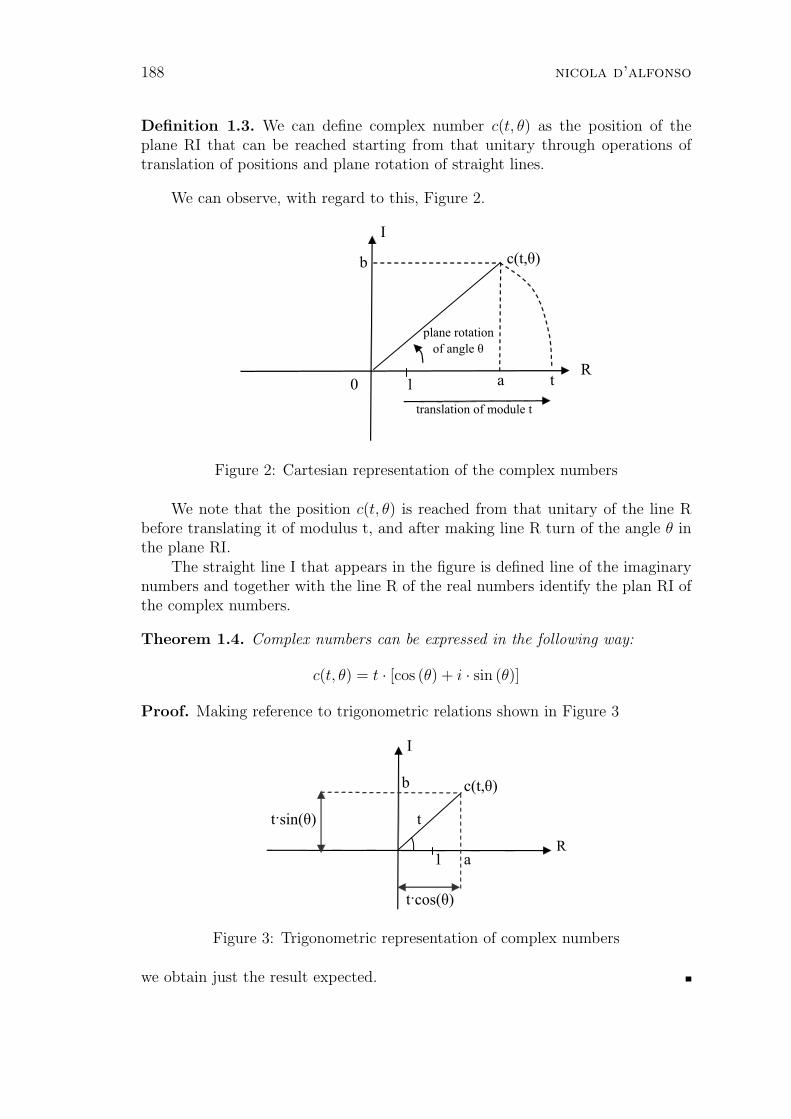
188 nicola d’alfonso
Definition 1.3. We can define complex number c(t, θ) as the position of theplane RI that can be reached starting from that unitary through operations oftranslation of positions and plane rotation of straight lines.
We can observe, with regard to this, Figure 2.
Figure 2: Cartesian representation of the complex numbers
We note that the position c(t, θ) is reached from that unitary of the line Rbefore translating it of modulus t, and after making line R turn of the angle θ inthe plane RI.
The straight line I that appears in the figure is defined line of the imaginarynumbers and together with the line R of the real numbers identify the plan RI ofthe complex numbers.
Theorem 1.4. Complex numbers can be expressed in the following way:
c(t, θ) = t · [cos (θ) + i · sin (θ)]
Proof. Making reference to trigonometric relations shown in Figure 3
Figure 3: Trigonometric representation of complex numbers
we obtain just the result expected.

numbers in the n dimensional space 189
Definition 1.5. The symbol t that indicates the distance of a complex numberc(t, θ) from the origin is defined modulus.
Theorem 1.6. The modulus t has the following property:
t =√
a2 + b2
Proof. By using Pythagoras’ theorem on the triangle identified in Figure 3 onthe preceding page we can obtain the relation:
t2 = a2 + b2
from which results the previous one.
Definition 1.7. The symbol θ that expresses the rotation that has to undergothe line R to align itself with the straight line that joins c(t, θ) to the origin isdefined plane phase.
Theorem 1.8. The plane phase θ has the following property:
θ = arctan( b
a
)
Proof. Making reference again to the same triangle of Figure 3 on the facingpage we obtain the relation:
b
a= tan (θ)
from which results the previous one.
Theorem 1.9. Complex numbers can be expressed in the following way:
c(t, θ) = t · [cos (θ + k · 360) + i · sin (θ + k · 360)] for k = 0,±1,±2,±3 . . .
Proof. The proof is immediate and is a consequence of the periodicity of thefunctions sin() and cos().
Theorem 1.10. Complex numbers can be expressed in the following way:
c(t, θ) = c(a, b) = a + i · b
Proof. The proof is immediate and is a consequence of the bijection betweentranslation and rotation operations of values (t, θ) and the positions (a,b) of theplane RI.
For more information on complex numbers see [1], Chapter 3.The transition from the first dimension of the real numbers to the second
dimension of the complex numbers has required an operation of rotation. Byfurther extending this procedure will be possible to introduce the n dimensionalnumbers and define their operations.

190 nicola d’alfonso
2. Numbers in three dimensional space
2.1. Introduction to the complete numbers
Definition 2.1. We can define complete number o(t, θ, γ) as the position of thespace RIU that can be reached starting from that unitary through operations oftranslation of positions, of plane rotation of straight lines and spatial rotation ofplanes.
We can observe, with regard to this, Figure 4.
Figure 4: Cartesian representation of the complete numbers
We note that the position o(t, θ, γ) is reached from that unitary of the line Rbefore translating it of modulus t, after making line R turn of the angle γ in theplane RI, and finally making the whole plane RU turn of the angle θ.
The straight line U that appears in the figure is defined line of the outgoingnumbers and together with the line R of the real numbers and the line I of theimaginary numbers identify the space RIU of the complete numbers.
Theorem 2.2. Complete numbers can be expressed in the following way:
o(t, θ, γ) = t · [cos (γ) · cos (θ)] + i · [cos (γ) · sin (θ)] + u · [sin (γ)]Proof. Making reference to trigonometric relations shown in Figure 5 we obtainjust the result expected.
Definition 2.3. The symbol t that indicates the distance of a complete numbero(t, θ, γ) from the origin is defined modulus.
Theorem 2.4. The modulus t has the following property:
t =√
a2 + b2 + c2
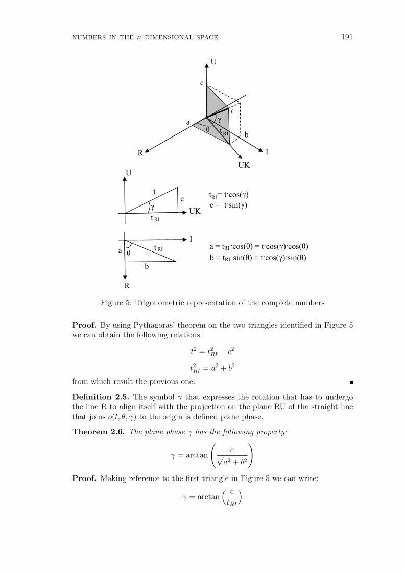
numbers in the n dimensional space 191
Figure 5: Trigonometric representation of the complete numbers
Proof. By using Pythagoras’ theorem on the two triangles identified in Figure 5we can obtain the following relations:
t2 = t2RI + c2
t2RI = a2 + b2
from which result the previous one.
Definition 2.5. The symbol γ that expresses the rotation that has to undergothe line R to align itself with the projection on the plane RU of the straight linethat joins o(t, θ, γ) to the origin is defined plane phase.
Theorem 2.6. The plane phase γ has the following property:
γ = arctan
(c√
a2 + b2
)
Proof. Making reference to the first triangle in Figure 5 we can write:
γ = arctan( c
tRI
)
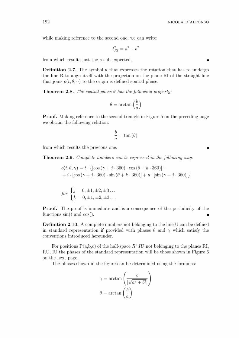
192 nicola d’alfonso
while making reference to the second one, we can write:
t2RI = a2 + b2
from which results just the result expected.
Definition 2.7. The symbol θ that expresses the rotation that has to undergothe line R to align itself with the projection on the plane RI of the straight linethat joins o(t, θ, γ) to the origin is defined spatial phase.
Theorem 2.8. The spatial phase θ has the following property:
θ = arctan( b
a
)
Proof. Making reference to the second triangle in Figure 5 on the preceding pagewe obtain the following relation:
b
a= tan (θ)
from which results the previous one.
Theorem 2.9. Complete numbers can be expressed in the following way:
o(t, θ, γ) = t · [cos (γ + j · 360) · cos (θ + k · 360)]+
+ i · [cos (γ + j · 360) · sin (θ + k · 360)] + u · [sin (γ + j · 360)]
for
j = 0,±1,±2,±3 . . .
k = 0,±1,±2,±3 . . .
Proof. The proof is immediate and is a consequence of the periodicity of thefunctions sin() and cos().
Definition 2.10. A complete numbers not belonging to the line U can be definedin standard representation if provided with phases θ and γ which satisfy theconventions introduced hereunder.
For positions P(a,b,c) of the half-space R+IU not belonging to the planes RI,RU, IU the phases of the standard representation will be those shown in Figure 6on the next page.
The phases shown in the figure can be determined using the formulas:
γ = arctan
(c
|√a2 + b2|
)
θ = arctan
(b
a
)
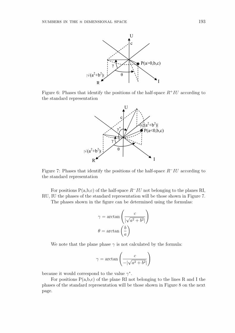
numbers in the n dimensional space 193
Figure 6: Phases that identify the positions of the half-space R+IU according tothe standard representation
Figure 7: Phases that identify the positions of the half-space R−IU according tothe standard representation
For positions P(a,b,c) of the half-space R−IU not belonging to the planes RI,RU, IU the phases of the standard representation will be those shown in Figure 7.
The phases shown in the figure can be determined using the formulas:
γ = arctan
(c
|√a2 + b2|
)
θ = arctan
(b
a
)
We note that the plane phase γ is not calculated by the formula:
γ = arctan
(c
−|√a2 + b2|
)
because it would correspond to the value γ∗.For positions P(a,b,c) of the plane RI not belonging to the lines R and I the
phases of the standard representation will be those shown in Figure 8 on the nextpage.

194 nicola d’alfonso
Figure 8: Phases that identify the positions of the plane RI according to thestandard representation
The phases shown in the figure can be determined using the formulas:
γ = arctan
(c√
a2 + b2
)
θ = arctan
(b
a
)
For positions P(a,b,c) of the half-plane R+U not belonging to the lines R andU the phases of the standard representation will be those shown in Figure 9.
Figure 9: Phases that identify the positions of the half-plane R+U according tothe standard representation
The phases shown in the figure can be determined using the formulas:
γ = arctan
(c
|a|)
θ = 0
For positions P(a,b,c) of the half-plane R−U not belonging to the lines R andU the phases of the standard representation will be those shown in Figure 10 onthe next page.
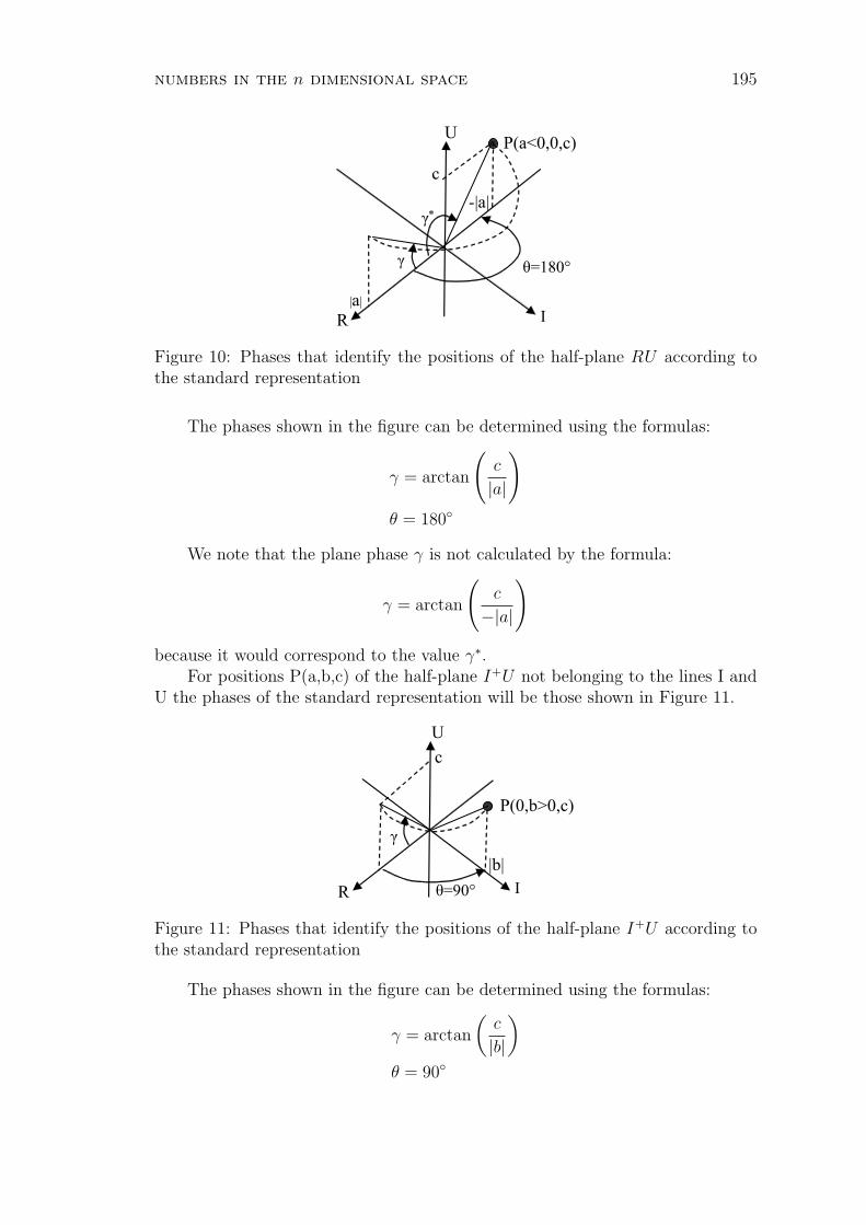
numbers in the n dimensional space 195
Figure 10: Phases that identify the positions of the half-plane RU according tothe standard representation
The phases shown in the figure can be determined using the formulas:
γ = arctan
(c
|a|
)
θ = 180
We note that the plane phase γ is not calculated by the formula:
γ = arctan
(c
−|a|
)
because it would correspond to the value γ∗.For positions P(a,b,c) of the half-plane I+U not belonging to the lines I and
U the phases of the standard representation will be those shown in Figure 11.
Figure 11: Phases that identify the positions of the half-plane I+U according tothe standard representation
The phases shown in the figure can be determined using the formulas:
γ = arctan
(c
|b|)
θ = 90
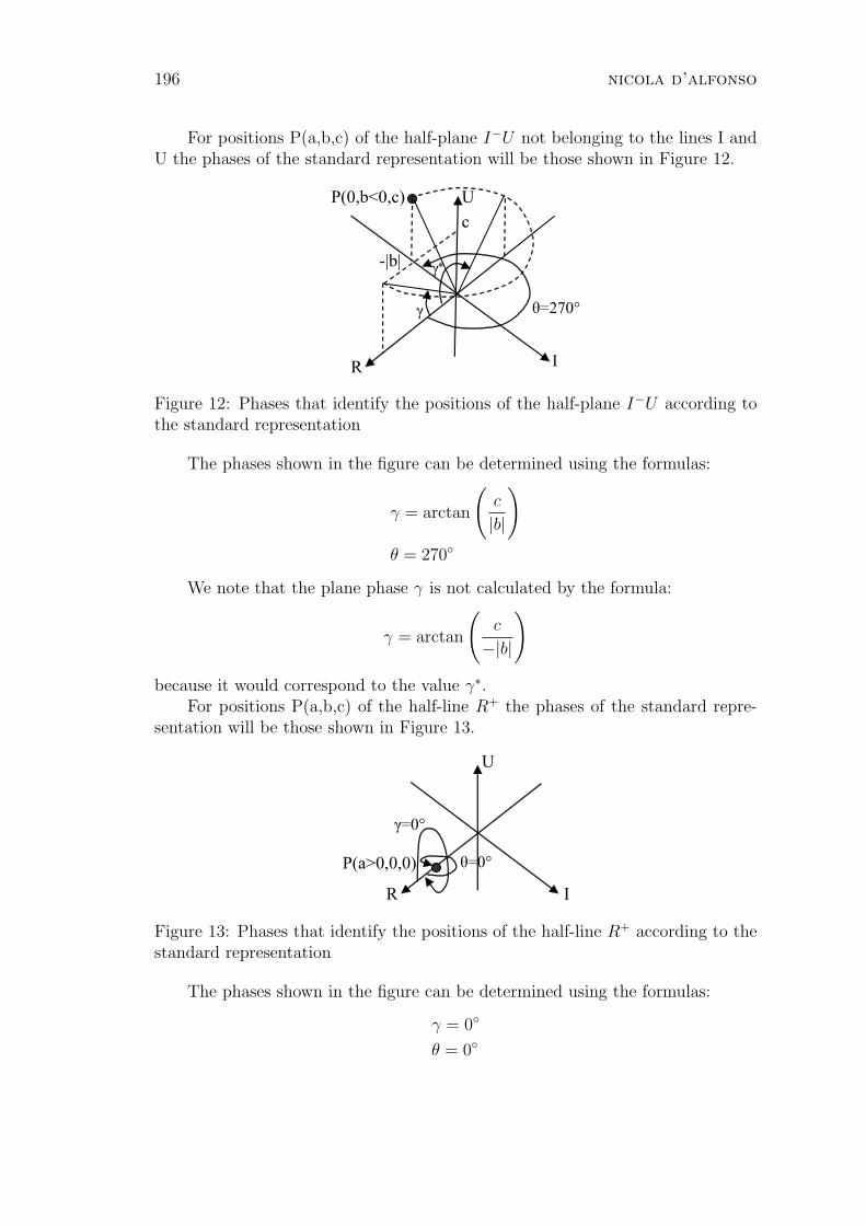
196 nicola d’alfonso
For positions P(a,b,c) of the half-plane I−U not belonging to the lines I andU the phases of the standard representation will be those shown in Figure 12.
Figure 12: Phases that identify the positions of the half-plane I−U according tothe standard representation
The phases shown in the figure can be determined using the formulas:
γ = arctan
(c
|b|
)
θ = 270
We note that the plane phase γ is not calculated by the formula:
γ = arctan
(c
−|b|
)
because it would correspond to the value γ∗.For positions P(a,b,c) of the half-line R+ the phases of the standard repre-
sentation will be those shown in Figure 13.
Figure 13: Phases that identify the positions of the half-line R+ according to thestandard representation
The phases shown in the figure can be determined using the formulas:
γ = 0
θ = 0
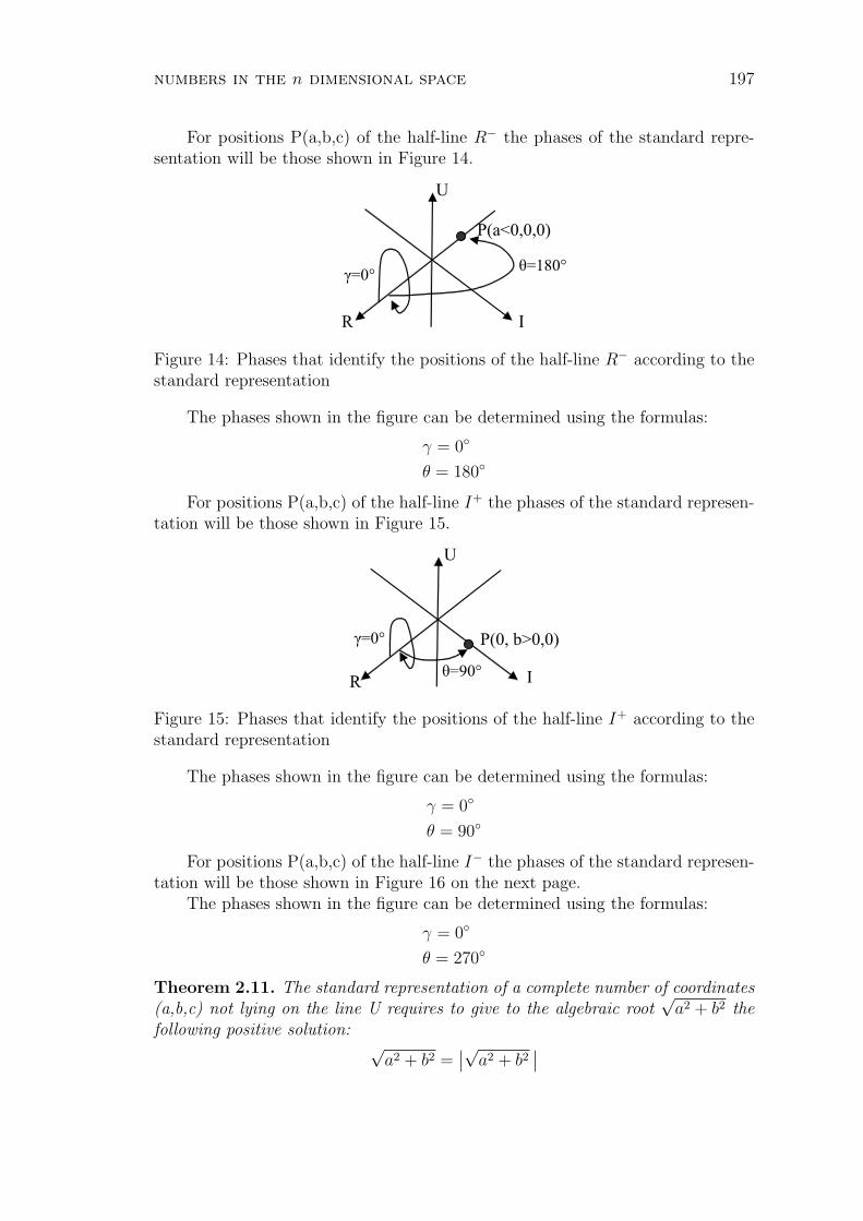
numbers in the n dimensional space 197
For positions P(a,b,c) of the half-line R− the phases of the standard repre-sentation will be those shown in Figure 14.
Figure 14: Phases that identify the positions of the half-line R− according to thestandard representation
The phases shown in the figure can be determined using the formulas:
γ = 0
θ = 180
For positions P(a,b,c) of the half-line I+ the phases of the standard represen-tation will be those shown in Figure 15.
Figure 15: Phases that identify the positions of the half-line I+ according to thestandard representation
The phases shown in the figure can be determined using the formulas:
γ = 0
θ = 90
For positions P(a,b,c) of the half-line I− the phases of the standard represen-tation will be those shown in Figure 16 on the next page.
The phases shown in the figure can be determined using the formulas:
γ = 0
θ = 270
Theorem 2.11. The standard representation of a complete number of coordinates(a,b,c) not lying on the line U requires to give to the algebraic root
√a2 + b2 the
following positive solution:√
a2 + b2 =∣∣√a2 + b2
∣∣
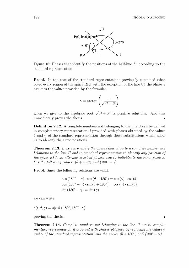
198 nicola d’alfonso
Figure 16: Phases that identify the positions of the half-line I− according to thestandard representation
Proof. In the case of the standard representations previously examined (thatcover every region of the space RIU with the exception of the line U) the phase γassumes the values provided by the formula:
γ = arctan
(c√
a2 + b2
)
when we give to the algebraic root√
a2 + b2 its positive solutions. And thisimmediately proves the thesis.
Definition 2.12. A complete numbers not belonging to the line U can be definedin complementary representation if provided with phases obtained by the valuesθ and γ of the standard representation through those substitutions which allowus to identify the same positions.
Theorem 2.13. If we call θ and γ the phases that allow to a complete number notbelonging to the line U and in standard representation to identify any position ofthe space RIU, an alternative set of phases able to individuate the same positionhas the following values: (θ + 180) and (180 − γ).
Proof. Since the following relations are valid:
cos (180 − γ) · cos (θ + 180) = cos (γ) · cos (θ)
cos (180 − γ) · sin (θ + 180) = cos (γ) · sin (θ)
sin (180 − γ) = sin (γ)
we can write:
o(t, θ, γ) = o(t, θ+180, 180−γ)
proving the thesis.
Theorem 2.14. Complete numbers not belonging to the line U are in comple-mentary representation if provided with phases obtained by replacing the values θand γ of the standard representation with the values (θ + 180) and (180 − γ).

numbers in the n dimensional space 199
Proof. The definition of the complete numbers in complementary representationand the theorem 2.13 directly prove the thesis.
Making reference to what we saw for the standard representation, the con-ventions adopted for the phases of the complementary representation will be thoseintroduced hereunder.
For positions P(a,b,c) of the half-space R+IU not belonging to the planes RI,RU, IU the phases of the complementary representation will be those shown inFigure 17.
Figure 17: Phases that identify the positions of the half-space R+IU according tothe complementary representation
The phases shown in the figure can be determined using the formulas:
γ = arctan
(c
−|√a2 + b2|
)
θ = arctan
(−b
−a
)
We note that the plane phase γ and the spatial phase θ are not calculated bythe formulas:
γ = arctan
(c
|√a2 + b2|
)
θ = arctan
(b
a
)
because they would correspond to the values γ∗ and θ∗.For positions P(a,b,c) of the half-space R−IU not belonging to the planes RI,
RU, IU the phases of the complementary representation will be those shown inFigure 18 on the next page.
The phases shown in the figure can be determined using the formulas:
γ = arctan
(c
−|√a2 + b2|
)
θ = arctan
(−b
−a
)
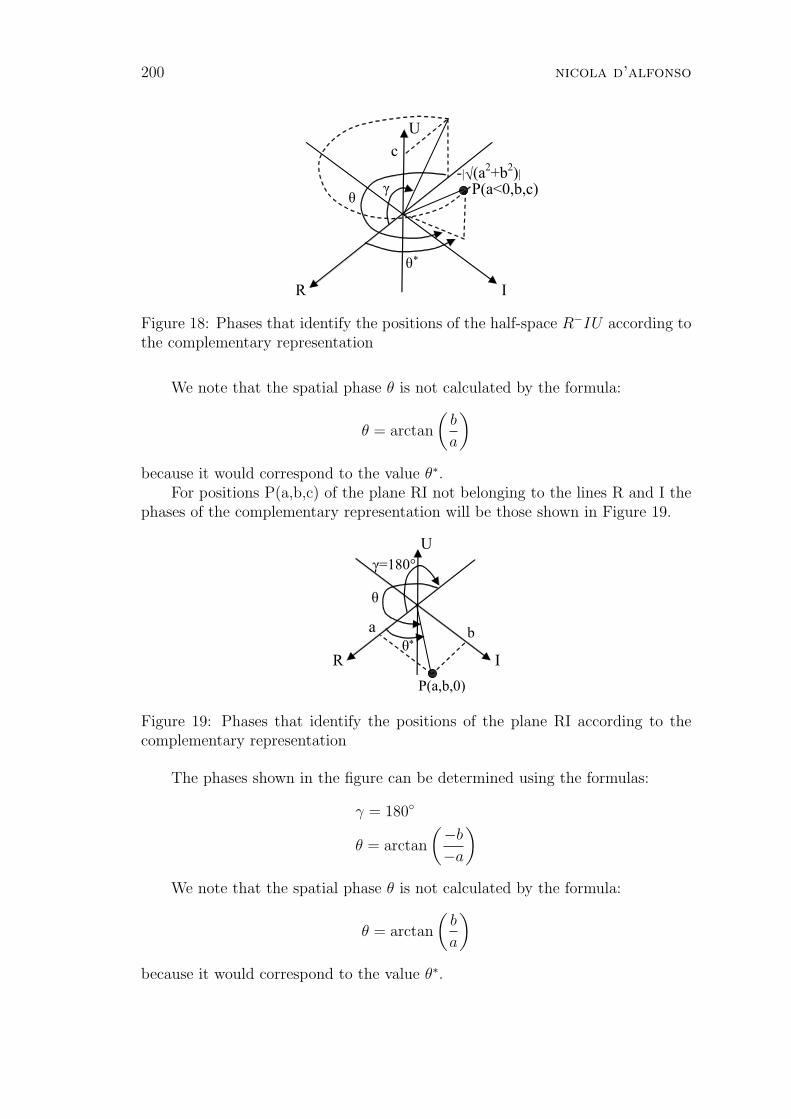
200 nicola d’alfonso
Figure 18: Phases that identify the positions of the half-space R−IU according tothe complementary representation
We note that the spatial phase θ is not calculated by the formula:
θ = arctan
(b
a
)
because it would correspond to the value θ∗.For positions P(a,b,c) of the plane RI not belonging to the lines R and I the
phases of the complementary representation will be those shown in Figure 19.
Figure 19: Phases that identify the positions of the plane RI according to thecomplementary representation
The phases shown in the figure can be determined using the formulas:
γ = 180
θ = arctan
(−b
−a
)
We note that the spatial phase θ is not calculated by the formula:
θ = arctan
(b
a
)
because it would correspond to the value θ∗.
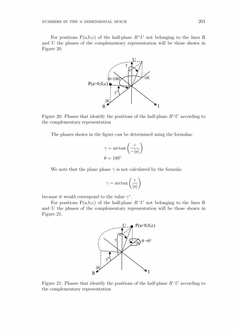
numbers in the n dimensional space 201
For positions P(a,b,c) of the half-plane R+U not belonging to the lines Rand U the phases of the complementary representation will be those shown inFigure 20.
Figure 20: Phases that identify the positions of the half-plane R+U according tothe complementary representation
The phases shown in the figure can be determined using the formulas:
γ = arctan
(c
−|a|)
θ = 180
We note that the plane phase γ is not calculated by the formula:
γ = arctan
(c
|a|)
because it would correspond to the value γ∗.For positions P(a,b,c) of the half-plane R−U not belonging to the lines R
and U the phases of the complementary representation will be those shown inFigure 21.
Figure 21: Phases that identify the positions of the half-plane R−U according tothe complementary representation
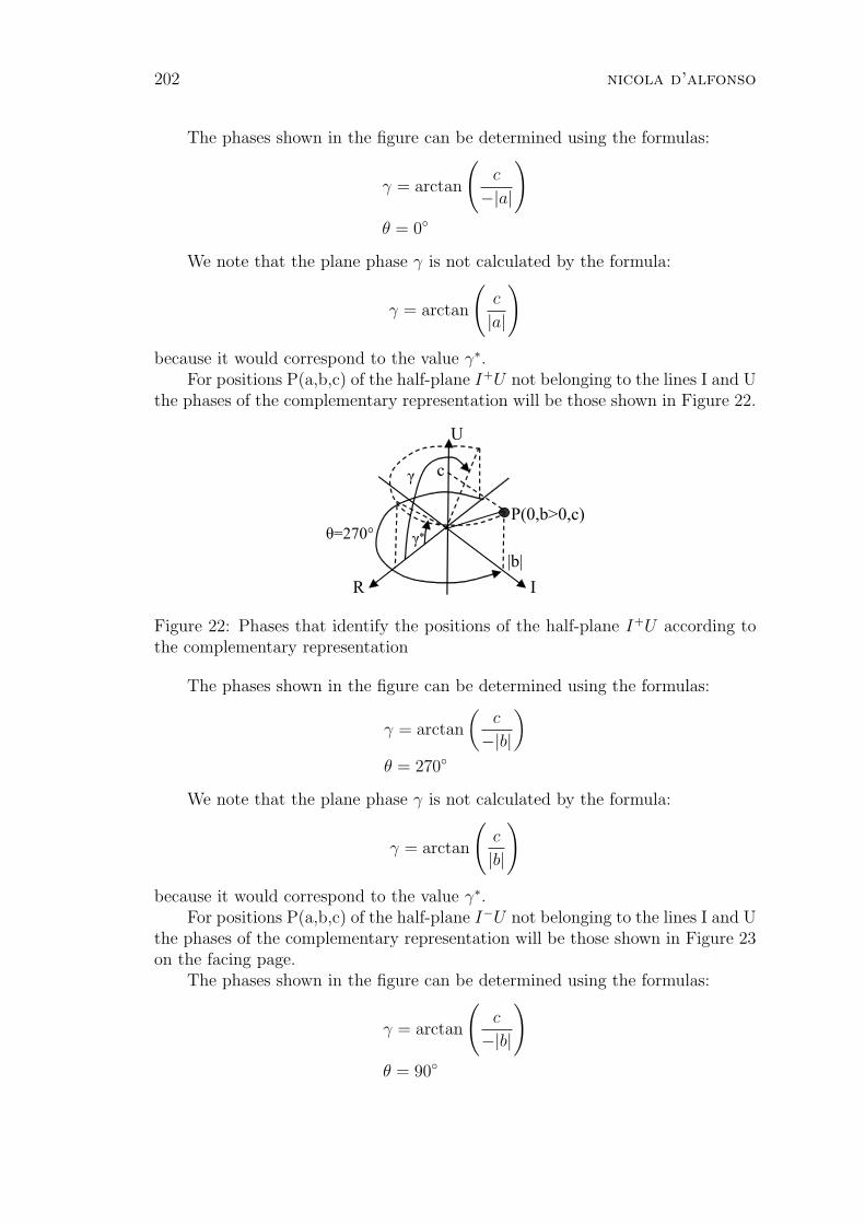
202 nicola d’alfonso
The phases shown in the figure can be determined using the formulas:
γ = arctan
(c
−|a|
)
θ = 0
We note that the plane phase γ is not calculated by the formula:
γ = arctan
(c
|a|
)
because it would correspond to the value γ∗.For positions P(a,b,c) of the half-plane I+U not belonging to the lines I and U
the phases of the complementary representation will be those shown in Figure 22.
Figure 22: Phases that identify the positions of the half-plane I+U according tothe complementary representation
The phases shown in the figure can be determined using the formulas:
γ = arctan
(c
−|b|)
θ = 270
We note that the plane phase γ is not calculated by the formula:
γ = arctan
(c
|b|
)
because it would correspond to the value γ∗.For positions P(a,b,c) of the half-plane I−U not belonging to the lines I and U
the phases of the complementary representation will be those shown in Figure 23on the facing page.
The phases shown in the figure can be determined using the formulas:
γ = arctan
(c
−|b|
)
θ = 90

numbers in the n dimensional space 203
Figure 23: Phases that identify the positions of the half-plane I−U according tothe complementary representation
We note that the plane phase γ is not calculated by the formula:
γ = arctan
(c
|b|
)
because it would correspond to the value γ∗.For positions P(a,b,c) of the half-line R+ the phases of the complementary
representation will be those shown in Figure 24.
Figure 24: Phases that identify the positions of the half-line R+ according to thecomplementary representation
The phases shown in the figure can be determined using the formulas:
γ = 180
θ = 180
For positions P(a,b,c) of the half-line R− the phases of the complementaryrepresentation will be those shown in Figure 25 on the following page.
The phases shown in the figure can be determined using the formulas:
γ = 180
θ = 0
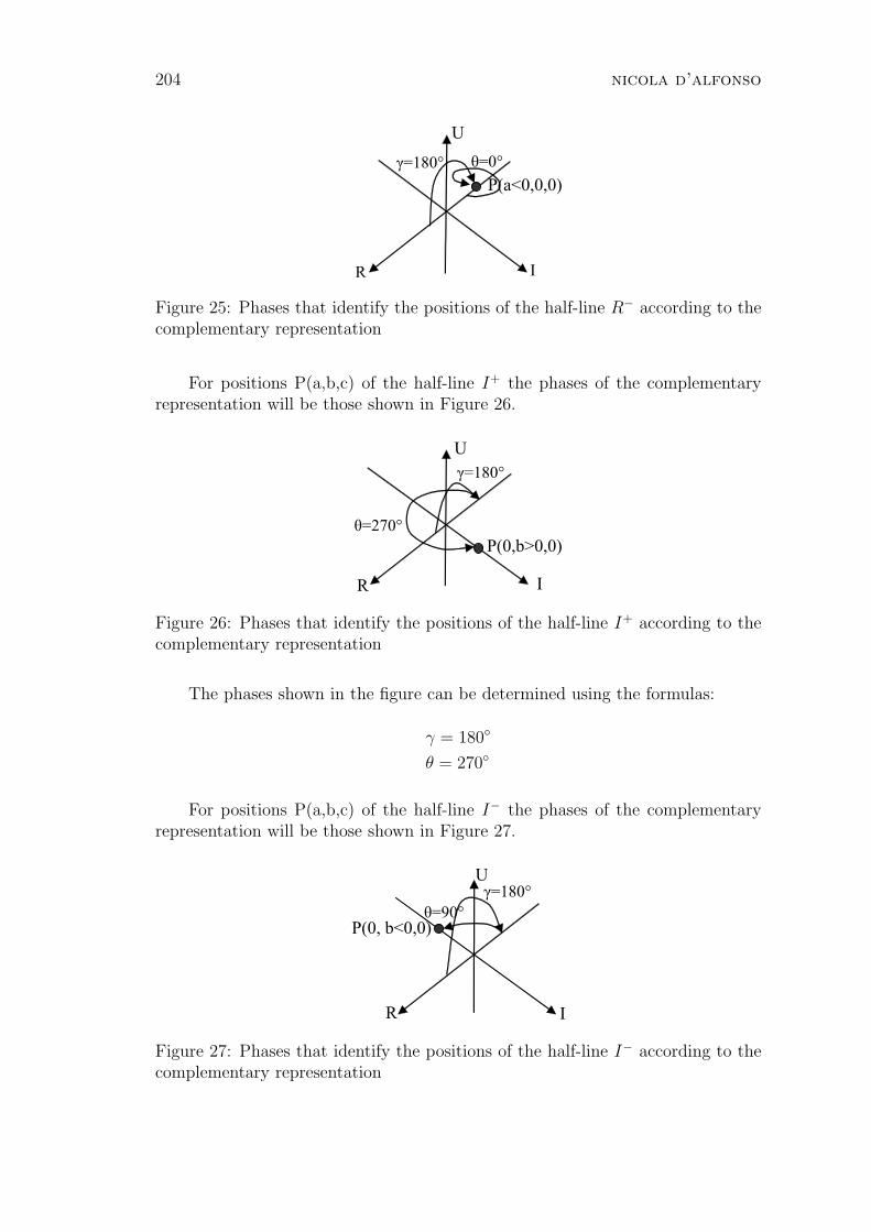
204 nicola d’alfonso
Figure 25: Phases that identify the positions of the half-line R− according to thecomplementary representation
For positions P(a,b,c) of the half-line I+ the phases of the complementaryrepresentation will be those shown in Figure 26.
Figure 26: Phases that identify the positions of the half-line I+ according to thecomplementary representation
The phases shown in the figure can be determined using the formulas:
γ = 180
θ = 270
For positions P(a,b,c) of the half-line I− the phases of the complementaryrepresentation will be those shown in Figure 27.
Figure 27: Phases that identify the positions of the half-line I− according to thecomplementary representation

numbers in the n dimensional space 205
The phases shown in the figure can be determined using the formulas:
γ = 180
θ = 90
Theorem 2.15. The complementary representation of a complete number of co-ordinates (a,b,c) not lying on the line U requires to give to the algebraic root√
a2 + b2 the following negative solution:√
a2 + b2 = −∣∣√a2 + b2
∣∣
Proof. In the case of the complementary representations previously examined(that cover every region of the space RIU with the exception of the line U) thephase γ assumes the values provided by the formula:
γ = arctan
(c√
a2 + b2
)
when we give to the algebraic root√
a2 + b2 its negative solutions. And thisimmediately proves the thesis.
Theorem 2.16. Each position of the line U corresponds to a complete numberfor each value assigned to the spatial phase θ.
Proof. By assigning at the expression of the complete numbers the valuesγ = ±90 that characterize the outgoing numbers of the line U:
o(t, θ,±90) = t · [cos (±90) · cos (θ)] + i · [cos (±90) · sin (θ)] + u · [sin (±90)]we obtain the same result regardless of the value of the spatial phase θ:
o(t, θ,±90) = t · u · [sin (±90)] = ±t · uproving the thesis.
Definition 2.17. A complete numbers belonging to the line U can be defined instandard representation if provided with spatial phase θ equal to zero.
Definition 2.18. A complete numbers belonging to the line U can be definedin complementary representation if provided with spatial phase θ different fromzero.
Since the non zero values of the spatial phase are unlimited, unlimited will alsobe the complementary representation related to the complete numbers belongingto the line U.
Theorem 2.19. Complex numbers cannot be expressed in the following way:
o(a, b, c) = a + i · b + u · cnamely:
o(t, θ, γ) 6= o(a, b, c) = a + i · b + u · c

206 nicola d’alfonso
Proof. The proof comes from the absence of bijection between translation androtation operations of values (t, θ, γ) and the positions (a,b,c) of the space RIU, asconfirmed by the existence of the complementary representation (Theorem 2.14).
Since it is impossible to associate the complete numbers to the individualpositions of the space, we can always express them in terms of their coordinates(a,b,c), provided that we make explicit the phases involved as well.
In other words we should use the following notation:
o(a, b, c)(t,θ,γ) = a(t) + i · b(θ) + u · c(γ)
where the values of t, θ, γ, if not yet given, should be reported to those whichcharacterize the standard representation.
However it is even possible to introduce a more concise notation by indicatingwhat representation is associate to the coordinates (a,b,c) or, in the case of theoutgoing numbers, the value of the spatial phase θ. In practice for the standardrepresentation we have:
o(a, b, c)(S) = (a + i · b + u · c)(S)
for the complementary representation:
o(a, b, c)(C) = (a + i · b + u · c)(C)
and finally for the outgoing numbers:
o(a, b, c)(θ) = u · c(θ)
While any other notation of the following type:
o(a, b, c) = a + i · b + u · cthat is devoid of sufficient information to trace the values of the phases θ and γ,will be able to represent the positions of the space RIU, but not the completenumbers.
2.2. Addition
Definition 2.20. In the space RIU we can define addition between two positionso1(a1, b1, c1) and o2(a2, b2, c2) as the position o1+2(a1+2, b1+2, c1+2) represented alsowith the symbol o1(a1, b1, c1) + o2(a2, b2, c2) that satisfies the following condition:
o1+2(a1+2, b1+2, c1+2) = o1+2(a1 + a2, b1 + b2, c1 + c2)
This condition is equivalent to take the position of the space RIU providedwith the following coordinates:
a1+2 = a1 + a2
b1+2 = b1 + b2
c1+2 = c1 + c2
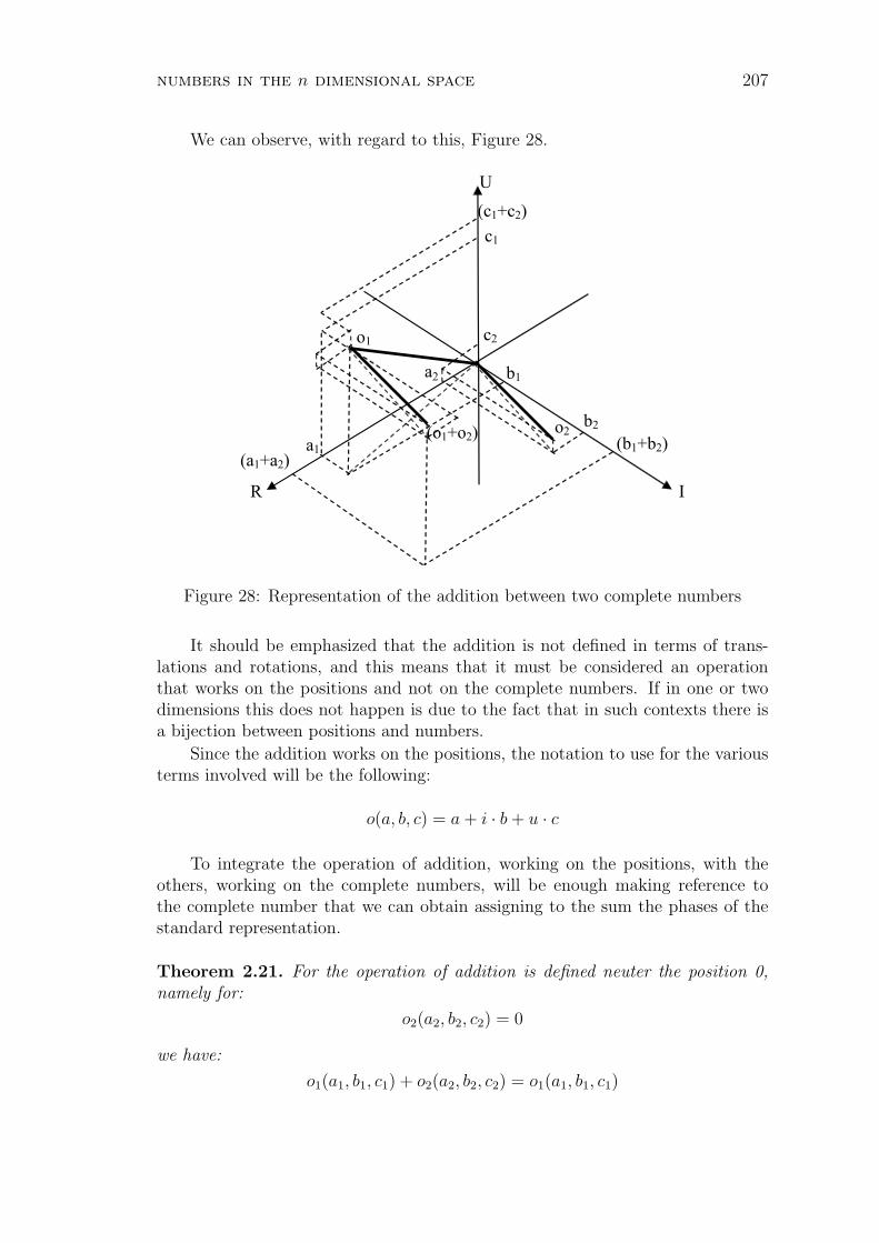
numbers in the n dimensional space 207
We can observe, with regard to this, Figure 28.
Figure 28: Representation of the addition between two complete numbers
It should be emphasized that the addition is not defined in terms of trans-lations and rotations, and this means that it must be considered an operationthat works on the positions and not on the complete numbers. If in one or twodimensions this does not happen is due to the fact that in such contexts there isa bijection between positions and numbers.
Since the addition works on the positions, the notation to use for the variousterms involved will be the following:
o(a, b, c) = a + i · b + u · c
To integrate the operation of addition, working on the positions, with theothers, working on the complete numbers, will be enough making reference tothe complete number that we can obtain assigning to the sum the phases of thestandard representation.
Theorem 2.21. For the operation of addition is defined neuter the position 0,namely for:
o2(a2, b2, c2) = 0
we have:
o1(a1, b1, c1) + o2(a2, b2, c2) = o1(a1, b1, c1)
208 nicola d’alfonso
Proof. a1,b1,c1,a2,b2,c2 being real numbers, we can write:
a1+2 = a1 + a2 = a1 + 0 = a1
b1+2 = b1 + b2 = b1 + 0 = b1
c1+2 = c1 + a2 = c1 + 0 = c1
proving the thesis.
Theorem 2.22. For the operation of addition is defined opposite the positionsymmetric with respect to the origin, namely for:
o2(a2, b2, c2) = o2(−a1,−b1,−c1)
we have:o1(a1, b1, c1) + o2(a2, b2, c2) = 0
Proof. a1,b1,c1,a2,b2,c2 being real numbers, we can write:
a1+2 = a1 + a2 = a1 − a1 = 0
b1+2 = b1 + b2 = b1 − b1 = 0
c1+2 = c1 + a2 = c1 − c1 = 0
proving the thesis.
Theorem 2.23. For the operation of addition is valid the commutative property,namely:
o1(a1, b1, c1) + o2(a2, b2, c2) = o2(a2, b2, c2) + o1(a1, b1, c1)
Proof. a1,b1,c1,a2,b2,c2 being real numbers, we can write:
a1+2 = a1 + a2
b1+2 = b1 + b2
c1+2 = c1 + c2
a2+1 = a2 + a1 = a1 + a2
b2+1 = b2 + b1 = b1 + b2
c2+1 = c2 + c1 = c1 + c2
proving the thesis.
Theorem 2.24. For the operation of addition are valid the associative and dis-sociative properties, namely for:
o2(a2, b2, c2) = o3(a3, b3, c3) + o4(a4, b4, c4)
we have:
o1(a1, b1, c1) + o2(a2, b2, c2) = [o1(a1, b1, c1) + o3(a3, b3, c3)] + o4(a4, b4, c4)
[o1(a1, b1, c1) + o3(a3, b3, c3)] + o4(a4, b4, c4) = o1(a1, b1, c1) + o2(a2, b2, c2)
numbers in the n dimensional space 209
Proof. a1,b1,c1,a2,b2,c2,a3,b3,c3,a4,b4,c4 being real numbers, we can write:
a1+2 = a1 + a2 = a1 + (a3 + a4) = (a1 + a3) + a4 = a(1+3)+4
b1+2 = b1 + b2 = b1 + (b3 + b4) = (b1 + b3) + b4 = b(1+3)+4
c1+2 = c1 + c2 = c1 + (c3 + c4) = (c1 + c3) + c4 = c(1+3)+4
a(1+3)+4 = (a1 + a3) + a4 = a1 + (a3 + a4) = a1 + a2 = a1+2
b(1+3)+4 = (b1 + b3) + b4 = b1 + (b3 + b4) = b1 + b2 = b1+2
c(1+3)+4 = (c1 + c3) + c4 = c1 + (c3 + c4) = c1 + a2 = c1+2
proving the thesis.
2.3. Subtraction
Definition 2.25. In the space RIU we can define subtraction between two po-sitions o1(a1, b1, c1) and o2(a2, b2, c2) as the position o1−2(a1−2, b1−2, c1−2) repre-sented also with the symbol o1(a1, b1, c1)− o2(a2, b2, c2) that satisfies the followingcondition:
o1−2(a1−2, b1−2, c1−2) + o2(a2, b2, c2) = o1(a1, b1, c1)
This condition defines the subtraction as the inverse operation of addition,and it is equivalent to require:
a1−2 = a1 − a2
b1−2 = b1 − b2
c1−2 = c1 − c2
It should be emphasized that the subtraction is not defined in terms of trans-lations and rotations, and this means that it must be considered an operationthat works on the positions and not on the complete numbers. If in one or twodimensions this does not happen is due to the fact that in such contexts there isa bijection between positions and numbers.
Since the subtraction works on the positions, the notation to use for thevarious terms involved will be the following:
o(a, b, c) = a + i · b + u · cTo integrate the operation of subtraction, working on the positions, with the
others, working on the complete numbers, will be enough making reference to thecomplete number that we can obtain assigning to the difference the phases of thestandard representation.
Theorem 2.26. For the operation of subtraction is defined neuter the position 0,namely for:
o2(a2, b2, c2) = 0
we have:o1(a1, b1, c1)− o2(a2, b2, c2) = o1(a1, b1, c1)

210 nicola d’alfonso
Proof. a1,b1,c1,a2,b2,c2 being real numbers, we can write:
a1−2 = a1 − a2 = a1 − 0 = a1
b1−2 = b1 − b2 = b1 − 0 = b1
c1−2 = c1 − a2 = c1 − 0 = c1
proving the thesis.
Theorem 2.27. For the operation of subtraction is defined identical, the sameposition with respect to the origin, namely for:
o2(a2, b2, c2) = o2(a1, b1, c1)
we have:o1(a1, b1, c1)− o2(a2, b2, c2) = 0
Proof. a1,b1,c1,a2,b2,c2 being real numbers, we can write:
a1−2 = a1 − a2 = a1 − a1 = 0
b1−2 = b1 − b2 = b1 − b1 = 0
c1−2 = c1 − a2 = c1 − c1 = 0
proving the thesis.
Theorem 2.28. For the operation of subtraction is valid the invariantive property,namely:
o1(a1, b1, c1)− o2(a2, b2, c2) =[o1(a1, b1, c1) + o3(a3, b3, c3)]+
− [o2(a2, b2, c2) + o3(a3, b3, c3)]
o1(a1, b1, c1)− o2(a2, b2, c2) =[o1(a1, b1, c1)− o3(a3, b3, c3)]+
− [o2(a2, b2, c2)− o3(a3, b3, c3)]
Proof. a1,b1,c1,a2,b2,c2,a3,b3,c3 being real numbers, we can write:
a1−2 = a1 − a2
b1−2 = b1 − b2
c1−2 = c1 − c2
a(1+3)−(2+3) = (a1 + a3)− (a2 + a3) = a1 + a3 − a2 − a3 = a1 − a2
b(1+3)−(2+3) = (b1 + b3)− (b2 + b3) = b1 + b3 − b2 − b3 = b1 − b2
c(1+3)−(2+3) = (c1 + c3)− (c2 + c3) = c1 + c3 − c2 − c3 = c1 − c2
a(1−3)−(2−3) = (a1 − a3)− (a2 − a3) = a1 − a3 − a2 + a3 = a1 − a2
b(1−3)−(2−3) = (b1 − b3)− (b2 − b3) = b1 − b3 − b2 + b3 = b1 − b2
c(1−3)−(2−3) = (c1 − c3)− (c2 − c3) = c1 − c3 − c2 + c3 = c1 − c2
proving the thesis.
numbers in the n dimensional space 211
Theorem 2.29. It is valid the equivalence between addition and subtraction,namely:
o1(a1, b1, c1) + o2(a2, b2, c2) = o1(a1, b1, c1)− [−o2(a2, b2, c2)]
o1(a1, b1, c1)− o2(a2, b2, c2) = o1(a1, b1, c1) + [−o2(a2, b2, c2)]
Proof. a1,b1,c1,a2,b2,c2 being real numbers, we can write:
a1+2 = a1 + a2
b1+2 = b1 + b2
c1+2 = c1 + c2
a1−(−2) = a1 − (−a2) = a1 + a2
b1−(−2) = b1 − (−b2) = b1 + b2
c1−(−2) = c1 − (−c2) = c1 + c2
a1−2 = a1 − a2
b1−2 = b1 − b2
c1−2 = c1 − c2
a1+(−2) = a1 + (−a2) = a1 − a2
b1+(−2) = b1 + (−b2) = b1 − b2
c1+(−2) = c1 + (−c2) = c1 − c2
proving the thesis.
2.4. Multiplication
Definition 2.30. In the space RIU we can define multiplication between twocomplete numbers o1(t1, θ1, γ1) and o2(t2, θ2, γ2) as the number o1·2(t1·2, θ1·2, γ1·2)represented also with the symbol o1(t1, θ1, γ1) · o2(t2, θ2, γ2) that satisfies the fol-lowing condition:
o1·2(t1·2, θ1·2, γ1·2) = o1·2(t1 · t2, θ1 + θ2, γ1 + γ2)
This condition defines the multiplication and it is equivalent to require:
t1·2 = t1 · t2θ1·2 = θ1 + θ2
γ1·2 = γ1 + γ2
We can observe, with regard to this, Figure 29 on the following page.
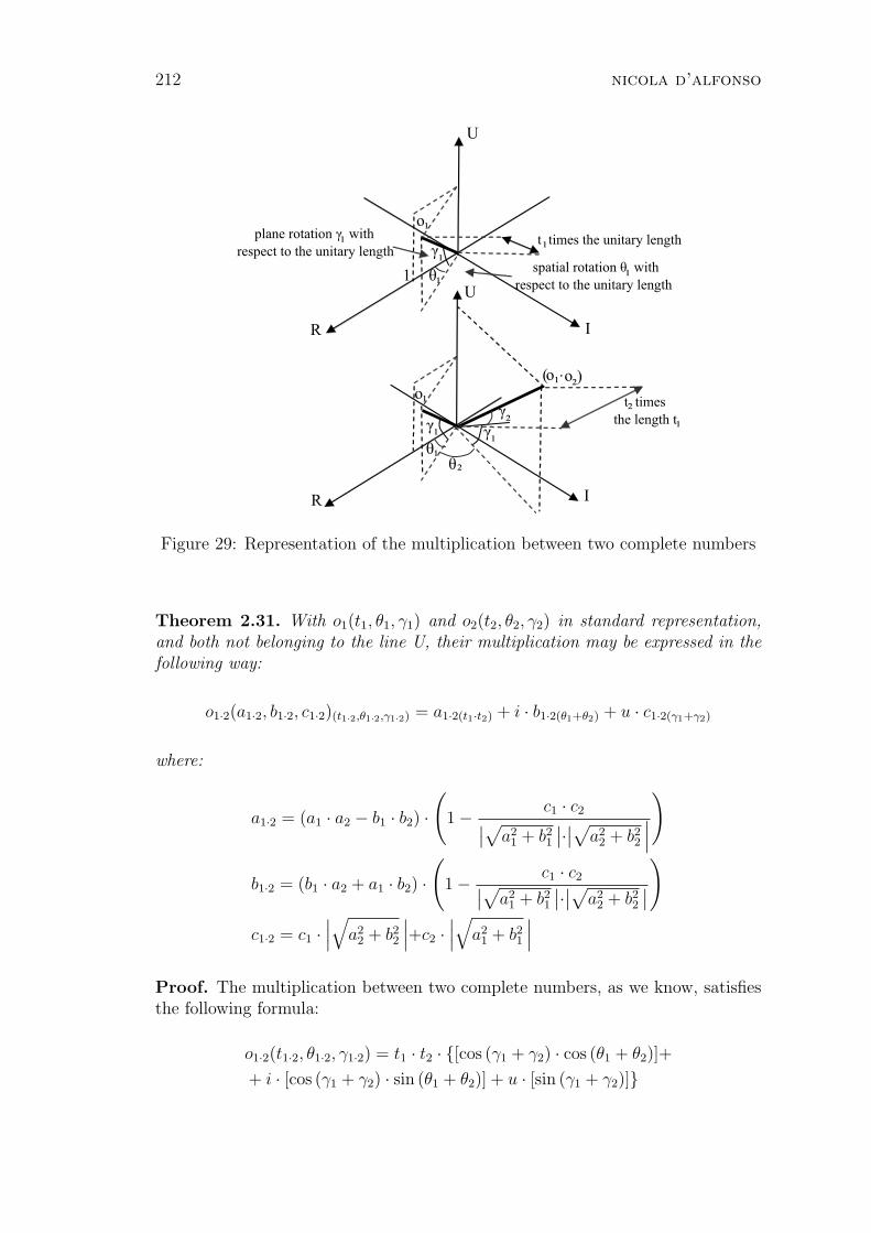
212 nicola d’alfonso
Figure 29: Representation of the multiplication between two complete numbers
Theorem 2.31. With o1(t1, θ1, γ1) and o2(t2, θ2, γ2) in standard representation,and both not belonging to the line U, their multiplication may be expressed in thefollowing way:
o1·2(a1·2, b1·2, c1·2)(t1·2,θ1·2,γ1·2) = a1·2(t1·t2) + i · b1·2(θ1+θ2) + u · c1·2(γ1+γ2)
where:
a1·2 = (a1 · a2 − b1 · b2) ·(
1− c1 · c2∣∣√a21 + b2
1
∣∣·∣∣√a2
2 + b22
∣∣∣
)
b1·2 = (b1 · a2 + a1 · b2) ·(
1− c1 · c2∣∣√a21 + b2
1
∣∣·∣∣√a2
2 + b22
∣∣
)
c1·2 = c1 ·∣∣∣√
a22 + b2
2
∣∣∣+c2 ·∣∣∣√
a21 + b2
1
∣∣∣
Proof. The multiplication between two complete numbers, as we know, satisfiesthe following formula:
o1·2(t1·2, θ1·2, γ1·2) = t1 · t2 · [cos (γ1 + γ2) · cos (θ1 + θ2)]+
+ i · [cos (γ1 + γ2) · sin (θ1 + θ2)] + u · [sin (γ1 + γ2)]
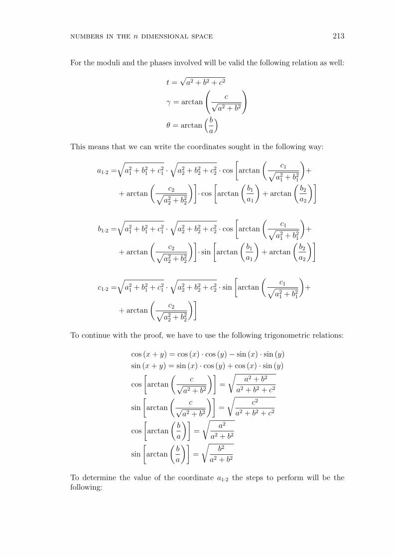
numbers in the n dimensional space 213
For the moduli and the phases involved will be valid the following relation as well:
t =√
a2 + b2 + c2
γ = arctan
(c√
a2 + b2
)
θ = arctan( b
a
)
This means that we can write the coordinates sought in the following way:
a1·2 =√
a21 + b2
1 + c21 ·
√a2
2 + b22 + c2
2 · cos
[arctan
(c1√
a21 + b2
1
)+
+ arctan
(c2√
a22 + b2
2
)]· cos
[arctan
(b1
a1
)+ arctan
(b2
a2
)]
b1·2 =√
a21 + b2
1 + c21 ·
√a2
2 + b22 + c2
2 · cos
[arctan
(c1√
a21 + b2
1
)+
+ arctan
(c2√
a22 + b2
2
)]· sin
[arctan
(b1
a1
)+ arctan
(b2
a2
)]
c1·2 =√
a21 + b2
1 + c21 ·
√a2
2 + b22 + c2
2 · sin[arctan
(c1√
a21 + b2
1
)+
+ arctan
(c2√
a22 + b2
2
)]
To continue with the proof, we have to use the following trigonometric relations:
cos (x + y) = cos (x) · cos (y)− sin (x) · sin (y)
sin (x + y) = sin (x) · cos (y) + cos (x) · sin (y)
cos
[arctan
(c√
a2 + b2
)]=
√a2 + b2
a2 + b2 + c2
sin
[arctan
(c√
a2 + b2
)]=
√c2
a2 + b2 + c2
cos
[arctan
(b
a
)]=
√a2
a2 + b2
sin
[arctan
(b
a
)]=
√b2
a2 + b2
To determine the value of the coordinate a1·2 the steps to perform will be thefollowing:
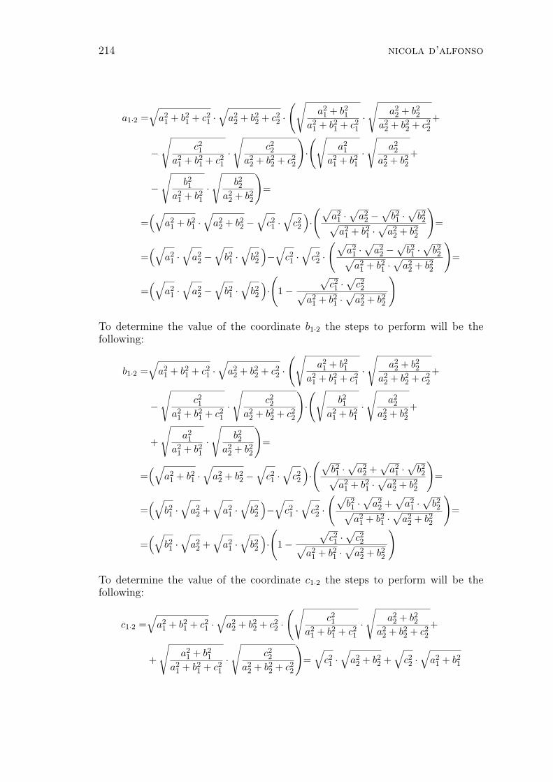
214 nicola d’alfonso
a1·2 =√
a21 + b2
1 + c21 ·
√a2
2 + b22 + c2
2 ·(√
a21 + b2
1
a21 + b2
1 + c21
·√
a22 + b2
2
a22 + b2
2 + c22
+
−√
c21
a21 + b2
1 + c21
·√
c22
a22 + b2
2 + c22
)·(√
a21
a21 + b2
1
·√
a22
a22 + b2
2
+
−√
b21
a21 + b2
1
·√
b22
a22 + b2
2
)=
=(√
a21 + b2
1 ·√
a22 + b2
2 −√
c21 ·
√c22
)·(√
a21 ·
√a2
2 −√
b21 ·
√b22√
a21 + b2
1 ·√
a22 + b2
2
)=
=(√
a21 ·
√a2
2 −√
b21 ·
√b22
)−
√c21 ·
√c22 ·
(√a2
1 ·√
a22 −
√b21 ·
√b22√
a21 + b2
1 ·√
a22 + b2
2
)=
=(√
a21 ·
√a2
2 −√
b21 ·
√b22
)·(
1−√
c21 ·
√c22√
a21 + b2
1 ·√
a22 + b2
2
)
To determine the value of the coordinate b1·2 the steps to perform will be thefollowing:
b1·2 =√
a21 + b2
1 + c21 ·
√a2
2 + b22 + c2
2 ·(√
a21 + b2
1
a21 + b2
1 + c21
·√
a22 + b2
2
a22 + b2
2 + c22
+
−√
c21
a21 + b2
1 + c21
·√
c22
a22 + b2
2 + c22
)·(√
b21
a21 + b2
1
·√
a22
a22 + b2
2
+
+
√a2
1
a21 + b2
1
·√
b22
a22 + b2
2
)=
=(√
a21 + b2
1 ·√
a22 + b2
2 −√
c21 ·
√c22
)·(√
b21 ·
√a2
2 +√
a21 ·
√b22√
a21 + b2
1 ·√
a22 + b2
2
)=
=(√
b21 ·
√a2
2 +√
a21 ·
√b22
)−
√c21 ·
√c22 ·
(√b21 ·
√a2
2 +√
a21 ·
√b22√
a21 + b2
1 ·√
a22 + b2
2
)=
=(√
b21 ·
√a2
2 +√
a21 ·
√b22
)·(
1−√
c21 ·
√c22√
a21 + b2
1 ·√
a22 + b2
2
)
To determine the value of the coordinate c1·2 the steps to perform will be thefollowing:
c1·2 =√
a21 + b2
1 + c21 ·
√a2
2 + b22 + c2
2 ·(√
c21
a21 + b2
1 + c21
·√
a22 + b2
2
a22 + b2
2 + c22
+
+
√a2
1 + b21
a21 + b2
1 + c21
·√
c22
a22 + b2
2 + c22
)=
√c21 ·
√a2
2 + b22 +
√c22 ·
√a2
1 + b21

numbers in the n dimensional space 215
These relations are valid in general, in the precise sense that they are also ableto include cases where the coefficients a,b,c are zero (provided that we work withcomplete numbers not belonging in the line U). But their main peculiarity is thatto contain many roots of the form
√x2.
Since the radicand x2 is always positive we know that the operation of alge-braic root considered here is permitted, and therefore it will be able to take asresult two opposite values: one positive and one negative. This means that frommathematical point of view we obtain a relation able to satisfies the multiplicationrule for each possible combination of signs attributable to the roots involved.
For example if we adopt the convention of attributing to the roots always thepositive value, we obtain the following result:
√a2 = |a|√b2 = |b|√c2 = |c|
to which correspond relations able to satisfy the multiplication role as a function ofthe modulus of the coordinates involved. This means that distinct complete num-bers will be able to give the same result of the multiplication if their coordinateswill have the same modulus.
Wanting to find relations that satisfy the multiplication rule as a function ofthe effective coordinates of the complete numbers involved, we must assign to theroots the same sign of the coefficient located within them:
√a2 = a√b2 = b√c2 = c
The relations obtained will be the following:
a1·2 = (a1 · a2 − b1 · b2) ·(
1− c1 · c2√a2
1 + b21 ·
√a2
2 + b22
)
b1·2 = (b1 · a2 + a1 · b2) ·(
1− c1 · c2√a2
1 + b21 ·
√a2
2 + b22
)
c1·2 = c1 ·√
a22 + b2
2 + c2 ·√
a21 + b2
1
(2.1)
Since the complete numbers involved are in standard representation, as de-termined by the theorem 2.11 we must consider the following relations:
√a2
1 + b21 =
∣∣√
a21 + b2
1
∣∣√
a22 + b2
2 =∣∣√
a22 + b2
2
∣∣
that combined with those indicated by the formulas (2.1), proving the thesis.
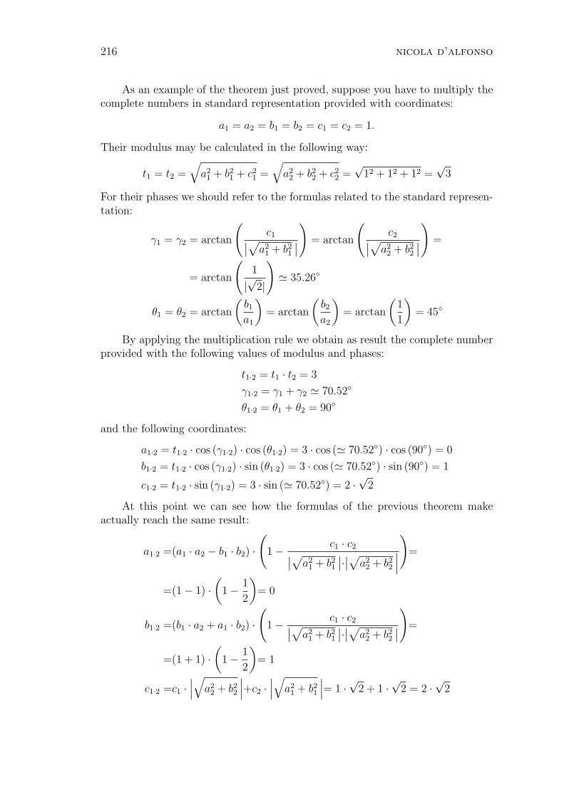
216 nicola d’alfonso
As an example of the theorem just proved, suppose you have to multiply thecomplete numbers in standard representation provided with coordinates:
a1 = a2 = b1 = b2 = c1 = c2 = 1.
Their modulus may be calculated in the following way:
t1 = t2 =√
a21 + b2
1 + c21 =
√a2
2 + b22 + c2
2 =√
12 + 12 + 12 =√
3
For their phases we should refer to the formulas related to the standard represen-tation:
γ1 = γ2 = arctan
(c1∣∣√a21 + b2
1
∣∣
)= arctan
(c2∣∣√a22 + b2
2
∣∣
)=
= arctan
(1
|√2|
)' 35.26
θ1 = θ2 = arctan
(b1
a1
)= arctan
(b2
a2
)= arctan
(1
1
)= 45
By applying the multiplication rule we obtain as result the complete numberprovided with the following values of modulus and phases:
t1·2 = t1 · t2 = 3
γ1·2 = γ1 + γ2 ' 70.52
θ1·2 = θ1 + θ2 = 90
and the following coordinates:
a1·2 = t1·2 · cos (γ1·2) · cos (θ1·2) = 3 · cos (' 70.52) · cos (90) = 0
b1·2 = t1·2 · cos (γ1·2) · sin (θ1·2) = 3 · cos (' 70.52) · sin (90) = 1
c1·2 = t1·2 · sin (γ1·2) = 3 · sin (' 70.52) = 2 ·√
2
At this point we can see how the formulas of the previous theorem makeactually reach the same result:
a1·2 =(a1 · a2 − b1 · b2) ·(
1− c1 · c2∣∣√a21 + b2
1
∣∣·∣∣√a2
2 + b22
∣∣∣
)=
=(1− 1) ·(
1− 1
2
)= 0
b1·2 =(b1 · a2 + a1 · b2) ·(
1− c1 · c2∣∣√a21 + b2
1
∣∣·∣∣√a2
2 + b22
∣∣
)=
=(1 + 1) ·(
1− 1
2
)= 1
c1·2 =c1 ·∣∣∣√
a22 + b2
2
∣∣∣+c2 ·∣∣∣√
a21 + b2
1
∣∣∣= 1 ·√
2 + 1 ·√
2 = 2 ·√
2
numbers in the n dimensional space 217
Theorem 2.32. With o1(t1, θ1, γ1) and o2(t2, θ2, γ2) in complementary represen-tation, and both not belonging to the line U, their multiplication may be expressedin the following way:
o1·2(a1·2, b1·2, c1·2)(t1·2,θ1·2,γ1·2) = a1·2(t1·t2) + i · b1·2(θ1+θ2) + u · c1·2(γ1+γ2)
where:
a1·2 = (a1 · a2 − b1 · b2) ·(
1− c1 · c2∣∣√a21 + b2
1
∣∣·∣∣√a2
2 + b22
∣∣∣
)
b1·2 = (b1 · a2 + a1 · b2) ·(
1− c1 · c2∣∣√a21 + b2
1
∣∣·∣∣√a2
2 + b22
∣∣∣
)
c1·2 = −c1 ·∣∣∣√
a22 + b2
2
∣∣∣−c2 ·∣∣∣√
a21 + b2
1
∣∣∣Proof. Since the complete numbers involved are in complementary representa-tion, as determined by the theorem 2.15 we must consider the following relations:
√a2
1 + b21 = −
∣∣√
a21 + b2
1
∣∣√
a22 + b2
2 = −∣∣√
a22 + b2
2
∣∣
that combined with those indicated by the formulas (2.1), proving the thesis.
As an example of the theorem just proved, suppose you have to multiply thecomplete numbers in complementary representation provided with coordinates:a1 = a2 = b1 = b2 = c1 = c2 = 1.
Their modulus may be calculated in the following way:
t1 = t2 =√
a21 + b2
1 + c21 =
√a2
2 + b22 + c2
2 =√
12 + 12 + 12 =√
3
For their phases we should refer to the formulas related to the complementaryrepresentation:
γ1 = γ2 = arctan
(c1
−∣∣√a2
1 + b21
∣∣
)= arctan
(c2
−∣∣√a2
2 + b22
∣∣
)=
= arctan
(1
−|√2|
)' 144.73
θ1 = θ2 = arctan
(−b1
−a1
)= arctan
(−b2
−a2
)= arctan
(−1
−1
)= 225
By applying the multiplication rule we obtain as result the complete numberprovided with the following values of modulus and phases:
t1·2 = t1 · t2 = 3
γ1·2 = γ1 + γ2 ' 289.46
θ1·2 = θ1 + θ2 = 450 = 90
218 nicola d’alfonso
and the following coordinates:
a1·2 = t1·2 · cos (γ1·2) · cos (θ1·2) = 3 · cos (' 289.46) · cos (90) = 0
b1·2 = t1·2 · cos (γ1·2) · sin (θ1·2) = 3 · cos (' 289.46) · sin (90) = 1
c1·2 = t1·2 · sin (γ1·2) = 3 · sin (' 289.46) = −2 ·√
2
At this point we can see how the formulas of the previous theorem makeactually reach the same result:
a1·2 = (a1 · a2 − b1 · b2) ·(
1− c1 · c2∣∣√a21 + b2
1
∣∣·∣∣√a2
2 + b22
∣∣∣
)=
= (1− 1) ·(
1− 1
2
)= 0
b1·2 = (b1 · a2 + a1 · b2) ·(
1− c1 · c2∣∣√a21 + b2
1
∣∣·∣∣√a2
2 + b22
∣∣
)=
= (1 + 1) ·(
1− 1
2
)= 1
c1·2 = −c1 ·∣∣∣√
a22 + b2
2
∣∣∣−c2 ·∣∣∣√
a21 + b2
1
∣∣∣= −1 ·√
2− 1 ·√
2 = −2 ·√
2
Theorem 2.33. With o1(t1, θ1, γ1) in standard representation and o2(t2, θ2, γ2) incomplementary representation, and both not belonging to the line U, their multi-plication may be expressed in the following way:
o1·2(a1·2, b1·2, c1·2)(t1·2,θ1·2,γ1·2) = a1·2(t1·t2) + i · b1·2(θ1+θ2) + u · c1·2(γ1+γ2)
where:
a1·2 = (a1 · a2 − b1 · b2) ·(
1 +c1 · c2∣∣√a2
1 + b21
∣∣·∣∣√a2
2 + b22
∣∣∣
)
b1·2 = (b1 · a2 + a1 · b2) ·(
1 +c1 · c2∣∣√a2
1 + b21
∣∣·∣∣√a2
2 + b22
∣∣∣
)
c1·2 = c2 ·∣∣∣√
a21 + b2
1
∣∣∣−c1 ·∣∣∣√
a22 + b2
2
∣∣∣
Proof. Since the first factor is in standard representation, as determined by thetheorem 2.11 we must consider the following relation:
√a2
1 + b21 =
∣∣√
a21 + b2
1
∣∣
while being the second factor in complementary representation, as determined bythe theorem 2.15 we must consider the following relation:
√a2
2 + b22 = −∣∣
√a2
2 + b22
∣∣
numbers in the n dimensional space 219
that combined with those indicated by the formulas (2.1), proving the thesis.As an example of the theorem just proved, suppose you have to multiply
the complete number in standard representation provided with coordinates a1 =b1 = c1 = 1 by that in complementary representation provided with the samecoordinates coordinates: a2 = b2 = c2 = 1.
Their modulus may be calculated in the following way:
t1 = t2 =√
a21 + b2
1 + c21 =
√a2
2 + b22 + c2
2 =√
12 + 12 + 12 =√
3
For their phases we should refer to the formulas related to the standard andcomplementary representations:
γ1 = arctan
(c1∣∣√a21 + b2
1
∣∣
)= arctan
(1
|√2|
)' 35.26
γ2 = arctan
(c2
−∣∣√a2
2 + b22
∣∣
)= arctan
(1
−|√2|
)' 144.73
θ1 = arctan
(b1
a1
)= arctan
(1
1
)= 45
θ2 = arctan
(−b2
−a2
)= arctan
(−1
−1
)= 225
By applying the multiplication rule we obtain as result the complete numberprovided with the following values of modulus and phases:
t1·2 = t1 · t2 = 3
γ1·2 = γ1 + γ2 = 180
θ1·2 = θ1 + θ2 = 270
and the following coordinates:
a1·2 = t1·2 · cos (γ1·2) · cos (θ1·2) = 3 · cos (180) · cos (270) = 0
b1·2 = t1·2 · cos (γ1·2) · sin (θ1·2) = 3 · cos (180) · sin (270) = 3
c1·2 = t1·2 · sin (γ1·2) = 3 · sin (180) = 0
At this point we can see how the formulas of the previous theorem makeactually reach the same result:
a1·2 = (a1 · a2 − b1 · b2) ·(
1 +c1 · c2∣∣√a2
1 + b21
∣∣·∣∣√a2
2 + b22
∣∣∣
)
= (1− 1) ·(
1 +1
2
)= 0
b1·2 = (b1 · a2 + a1 · b2) ·(
1 +c1 · c2∣∣√a2
1 + b21
∣∣·∣∣√a2
2 + b22
∣∣
)
= (1 + 1) ·(
1 +1
2
)= 3
c1·2 = c2 ·∣∣∣√
a21 + b2
1
∣∣∣−c1 ·∣∣∣√
a22 + b2
2
∣∣∣= 1 ·√
2− 1 ·√
2 = 0
220 nicola d’alfonso
Theorem 2.34. With o1(t1, θ1, γ1) in complementary representation ando2(t2, θ2, γ2) in standard representation, and both not belonging to the line U, theirmultiplication may be expressed in the following way:
o1·2(a1·2, b1·2, c1·2)(t1·2,θ1·2,γ1·2) = a1·2(t1·t2) + i · b1·2(θ1+θ2) + u · c1·2(γ1+γ2)
where:
a1·2 = (a1 · a2 − b1 · b2) ·(
1 +c1 · c2∣∣√a2
1 + b21
∣∣·∣∣√a2
2 + b22
∣∣∣
)
b1·2 = (b1 · a2 + a1 · b2) ·(
1 +c1 · c2∣∣√a2
1 + b21
∣∣·∣∣√
a22 + b2
2
∣∣∣
)
c1·2 = c1 ·∣∣∣√
a22 + b2
2
∣∣∣−c2 ·∣∣∣√
a21 + b2
1
∣∣∣Proof. Since the first factor is in complementary representation, as determinedby the theorem 2.15 we must consider the following relation:
√a2
1 + b21 = −
∣∣√
a21 + b2
1
∣∣
while being the second factor in standard representation, as determined by thetheorem 2.11 we must consider the following relation:
√a2
2 + b22 =
∣∣√
a22 + b2
2
∣∣
that combined with those indicated by the formulas (2.1), proving the thesis.
As an example of the theorem just proved, suppose you have to multiplythe complete number in complementary representation provided with coordinatesa1 = b1 = c1 = 1 by that in standard representation provided with the samecoordinates coordinates: a2 = b2 = c2 = 1.
Their modulus may be calculated in the following way:
t1 = t2 =√
a21 + b2
1 + c21 =
√a2
2 + b22 + c2
2 =√
12 + 12 + 12 =√
3
For their phases we should refer to the formulas related to the complementaryand standard representations:
γ1 = arctan
(c1
−∣∣√a2
1 + b21
∣∣
)= arctan
(1
−|√2|
)' 144.73
γ2 = arctan
(c2∣∣√a22 + b2
2
∣∣
)= arctan
(1
|√2|
)' 35.26
θ1 = arctan
(−b1
−a1
)= arctan
(−1
−1
)= 225
θ2 = arctan
(b2
a2
)= arctan
(1
1
)= 45
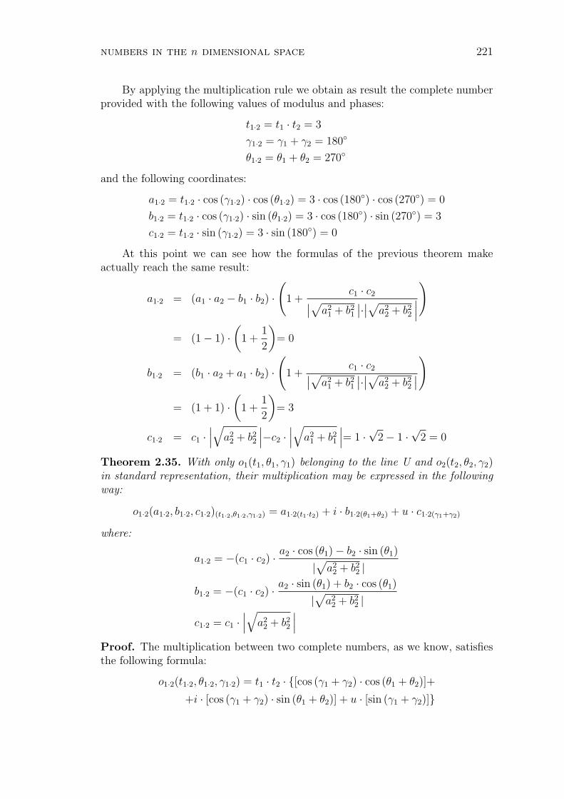
numbers in the n dimensional space 221
By applying the multiplication rule we obtain as result the complete numberprovided with the following values of modulus and phases:
t1·2 = t1 · t2 = 3
γ1·2 = γ1 + γ2 = 180
θ1·2 = θ1 + θ2 = 270
and the following coordinates:
a1·2 = t1·2 · cos (γ1·2) · cos (θ1·2) = 3 · cos (180) · cos (270) = 0
b1·2 = t1·2 · cos (γ1·2) · sin (θ1·2) = 3 · cos (180) · sin (270) = 3
c1·2 = t1·2 · sin (γ1·2) = 3 · sin (180) = 0
At this point we can see how the formulas of the previous theorem makeactually reach the same result:
a1·2 = (a1 · a2 − b1 · b2) ·(
1 +c1 · c2∣∣√a2
1 + b21
∣∣·∣∣√a2
2 + b22
∣∣∣
)
= (1− 1) ·(
1 +1
2
)= 0
b1·2 = (b1 · a2 + a1 · b2) ·(
1 +c1 · c2∣∣√a2
1 + b21
∣∣·∣∣√a2
2 + b22
∣∣
)
= (1 + 1) ·(
1 +1
2
)= 3
c1·2 = c1 ·∣∣∣√
a22 + b2
2
∣∣∣−c2 ·∣∣∣√
a21 + b2
1
∣∣∣= 1 ·√
2− 1 ·√
2 = 0
Theorem 2.35. With only o1(t1, θ1, γ1) belonging to the line U and o2(t2, θ2, γ2)in standard representation, their multiplication may be expressed in the followingway:
o1·2(a1·2, b1·2, c1·2)(t1·2,θ1·2,γ1·2) = a1·2(t1·t2) + i · b1·2(θ1+θ2) + u · c1·2(γ1+γ2)
where:
a1·2 = −(c1 · c2) · a2 · cos (θ1)− b2 · sin (θ1)
|√
a22 + b2
2 |b1·2 = −(c1 · c2) · a2 · sin (θ1) + b2 · cos (θ1)
|√
a22 + b2
2 |c1·2 = c1 ·
∣∣∣√
a22 + b2
2
∣∣∣Proof. The multiplication between two complete numbers, as we know, satisfiesthe following formula:
o1·2(t1·2, θ1·2, γ1·2) = t1 · t2 · [cos (γ1 + γ2) · cos (θ1 + θ2)]+
+i · [cos (γ1 + γ2) · sin (θ1 + θ2)] + u · [sin (γ1 + γ2)]
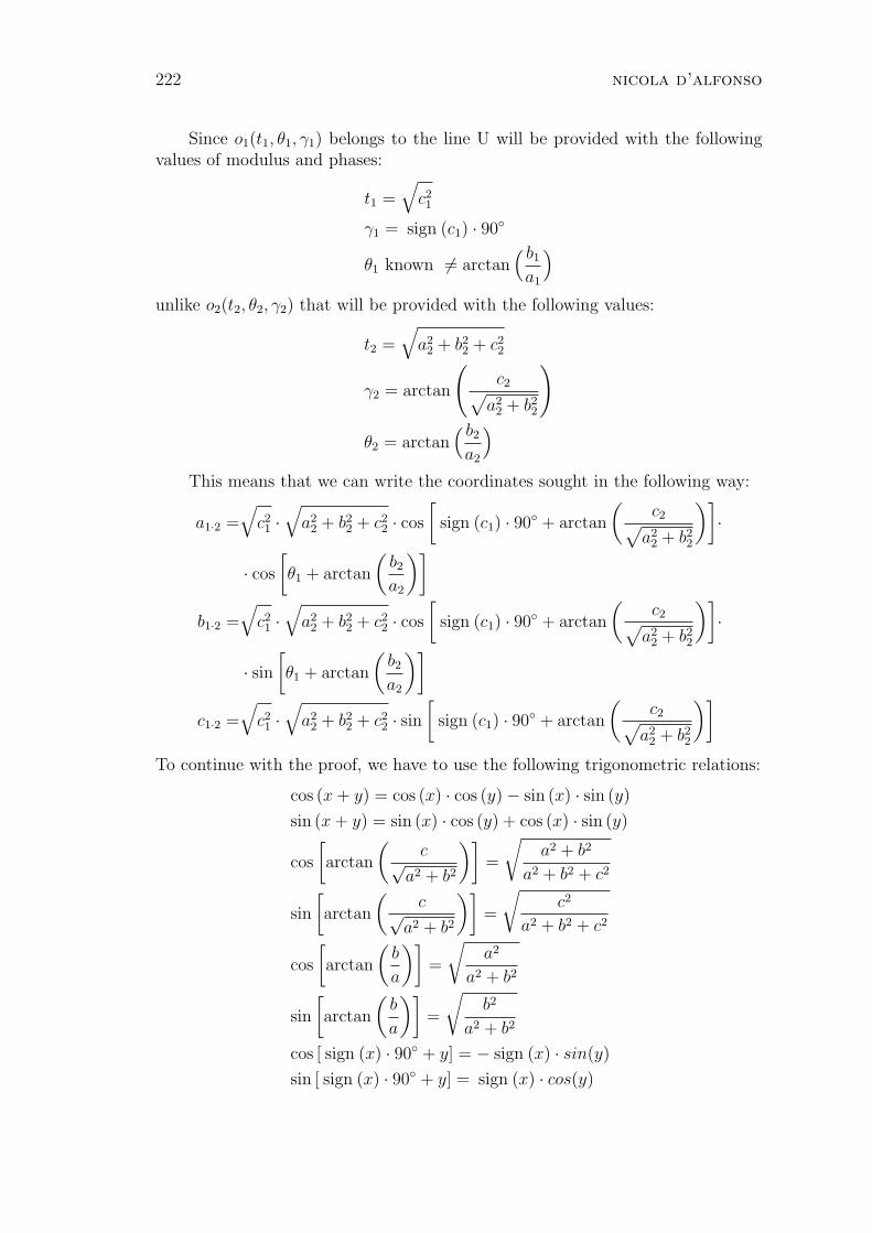
222 nicola d’alfonso
Since o1(t1, θ1, γ1) belongs to the line U will be provided with the followingvalues of modulus and phases:
t1 =√
c21
γ1 = sign (c1) · 90
θ1 known 6= arctan( b1
a1
)
unlike o2(t2, θ2, γ2) that will be provided with the following values:
t2 =√
a22 + b2
2 + c22
γ2 = arctan
(c2√
a22 + b2
2
)
θ2 = arctan( b2
a2
)
This means that we can write the coordinates sought in the following way:
a1·2 =√
c21 ·
√a2
2 + b22 + c2
2 · cos
[sign (c1) · 90 + arctan
(c2√
a22 + b2
2
)]·
· cos
[θ1 + arctan
(b2
a2
)]
b1·2 =√
c21 ·
√a2
2 + b22 + c2
2 · cos
[sign (c1) · 90 + arctan
(c2√
a22 + b2
2
)]·
· sin[θ1 + arctan
(b2
a2
)]
c1·2 =√
c21 ·
√a2
2 + b22 + c2
2 · sin[
sign (c1) · 90 + arctan
(c2√
a22 + b2
2
)]
To continue with the proof, we have to use the following trigonometric relations:
cos (x + y) = cos (x) · cos (y)− sin (x) · sin (y)
sin (x + y) = sin (x) · cos (y) + cos (x) · sin (y)
cos
[arctan
(c√
a2 + b2
)]=
√a2 + b2
a2 + b2 + c2
sin
[arctan
(c√
a2 + b2
)]=
√c2
a2 + b2 + c2
cos
[arctan
(b
a
)]=
√a2
a2 + b2
sin
[arctan
(b
a
)]=
√b2
a2 + b2
cos [ sign (x) · 90 + y] = − sign (x) · sin(y)
sin [ sign (x) · 90 + y] = sign (x) · cos(y)
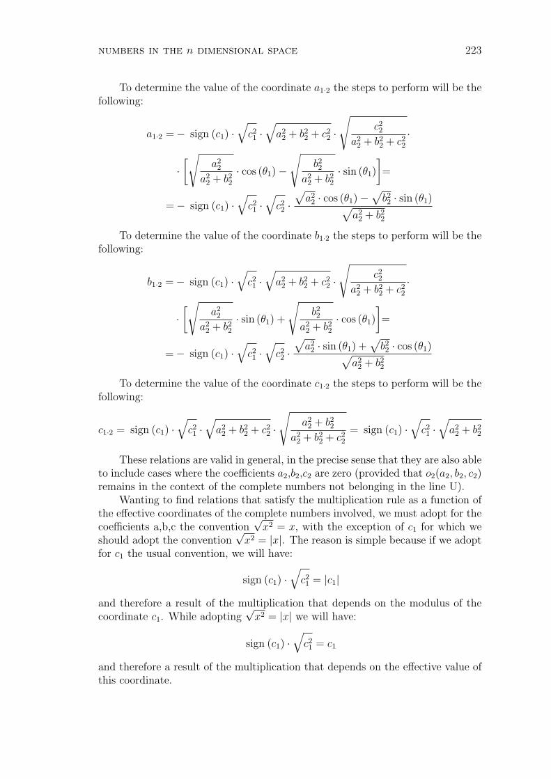
numbers in the n dimensional space 223
To determine the value of the coordinate a1·2 the steps to perform will be thefollowing:
a1·2 =− sign (c1) ·√
c21 ·
√a2
2 + b22 + c2
2 ·√
c22
a22 + b2
2 + c22
·
·[√
a22
a22 + b2
2
· cos (θ1)−√
b22
a22 + b2
2
· sin (θ1)
]=
=− sign (c1) ·√
c21 ·
√c22 ·
√a2
2 · cos (θ1)−√
b22 · sin (θ1)√
a22 + b2
2
To determine the value of the coordinate b1·2 the steps to perform will be thefollowing:
b1·2 =− sign (c1) ·√
c21 ·
√a2
2 + b22 + c2
2 ·√
c22
a22 + b2
2 + c22
·
·[√
a22
a22 + b2
2
· sin (θ1) +
√b22
a22 + b2
2
· cos (θ1)
]=
=− sign (c1) ·√
c21 ·
√c22 ·
√a2
2 · sin (θ1) +√
b22 · cos (θ1)√
a22 + b2
2
To determine the value of the coordinate c1·2 the steps to perform will be thefollowing:
c1·2 = sign (c1) ·√
c21 ·
√a2
2 + b22 + c2
2 ·√
a22 + b2
2
a22 + b2
2 + c22
= sign (c1) ·√
c21 ·
√a2
2 + b22
These relations are valid in general, in the precise sense that they are also ableto include cases where the coefficients a2,b2,c2 are zero (provided that o2(a2, b2, c2)remains in the context of the complete numbers not belonging in the line U).
Wanting to find relations that satisfy the multiplication rule as a function ofthe effective coordinates of the complete numbers involved, we must adopt for thecoefficients a,b,c the convention
√x2 = x, with the exception of c1 for which we
should adopt the convention√
x2 = |x|. The reason is simple because if we adoptfor c1 the usual convention, we will have:
sign (c1) ·√
c21 = |c1|
and therefore a result of the multiplication that depends on the modulus of thecoordinate c1. While adopting
√x2 = |x| we will have:
sign (c1) ·√
c21 = c1
and therefore a result of the multiplication that depends on the effective value ofthis coordinate.
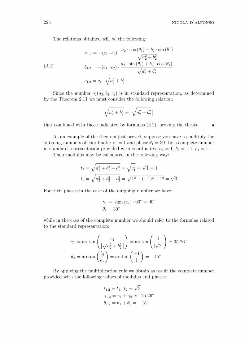
224 nicola d’alfonso
The relations obtained will be the following:
a1·2 = −(c1 · c2) · a2 · cos (θ1)− b2 · sin (θ1)√a2
2 + b22
b1·2 = −(c1 · c2) · a2 · sin (θ1) + b2 · cos (θ1)√a2
2 + b22
c1·2 = c1 ·√
a22 + b2
2
(2.2)
Since the number o2(a2, b2, c2) is in standard representation, as determinedby the Theorem 2.11 we must consider the following relation:
√a2
2 + b22 =
∣∣√
a22 + b2
2
∣∣
that combined with those indicated by formulas (2.2), proving the thesis.
As an example of the theorem just proved, suppose you have to multiply theoutgoing numbers of coordinate: c1 = 1 and phase θ1 = 30 by a complete numberin standard representation provided with coordinates: a2 = 1, b2 = −1, c2 = 1.
Their modulus may be calculated in the following way:
t1 =√
a21 + b2
1 + c21 =
√c21 =
√1 = 1
t2 =√
a22 + b2
2 + c22 =
√12 + (−1)2 + 12 =
√3
For their phases in the case of the outgoing number we have:
γ1 = sign (c1) · 90 = 90
θ1 = 30
while in the case of the complete number we should refer to the formulas relatedto the standard representation:
γ2 = arctan
(c2∣∣√a22 + b2
2
∣∣
)= arctan
(1
|√2|
)' 35.26
θ2 = arctan
(b2
a2
)= arctan
(−1
1
)= −45
By applying the multiplication rule we obtain as result the complete numberprovided with the following values of modulus and phases:
t1·2 = t1 · t2 =√
3
γ1·2 = γ1 + γ2 ' 125.26
θ1·2 = θ1 + θ2 = −15
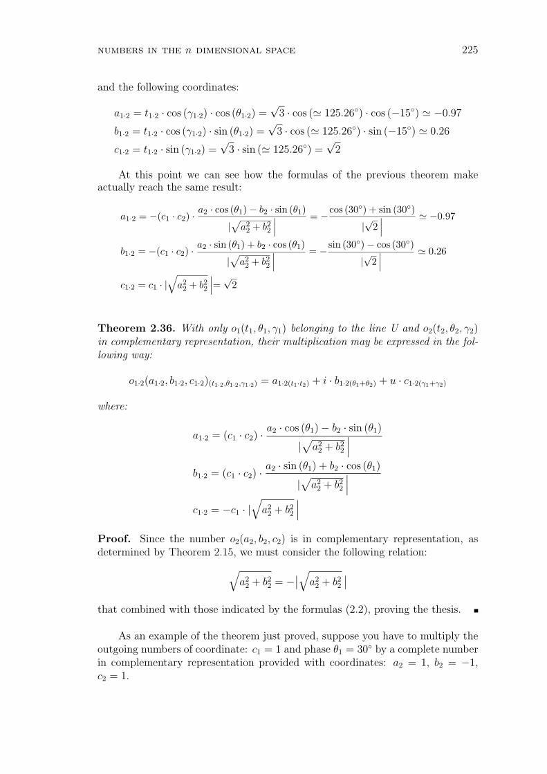
numbers in the n dimensional space 225
and the following coordinates:
a1·2 = t1·2 · cos (γ1·2) · cos (θ1·2) =√
3 · cos (' 125.26) · cos (−15) ' −0.97
b1·2 = t1·2 · cos (γ1·2) · sin (θ1·2) =√
3 · cos (' 125.26) · sin (−15) ' 0.26
c1·2 = t1·2 · sin (γ1·2) =√
3 · sin (' 125.26) =√
2
At this point we can see how the formulas of the previous theorem makeactually reach the same result:
a1·2 = −(c1 · c2) · a2 · cos (θ1)− b2 · sin (θ1)
|√
a22 + b2
2
∣∣∣= −cos (30) + sin (30)
|√2∣∣∣
' −0.97
b1·2 = −(c1 · c2) · a2 · sin (θ1) + b2 · cos (θ1)
|√
a22 + b2
2
∣∣∣= −sin (30)− cos (30)
|√2∣∣∣
' 0.26
c1·2 = c1 · |√
a22 + b2
2
∣∣∣=√
2
Theorem 2.36. With only o1(t1, θ1, γ1) belonging to the line U and o2(t2, θ2, γ2)in complementary representation, their multiplication may be expressed in the fol-lowing way:
o1·2(a1·2, b1·2, c1·2)(t1·2,θ1·2,γ1·2) = a1·2(t1·t2) + i · b1·2(θ1+θ2) + u · c1·2(γ1+γ2)
where:
a1·2 = (c1 · c2) · a2 · cos (θ1)− b2 · sin (θ1)
|√
a22 + b2
2
∣∣∣
b1·2 = (c1 · c2) · a2 · sin (θ1) + b2 · cos (θ1)
|√
a22 + b2
2
∣∣∣
c1·2 = −c1 · |√
a22 + b2
2
∣∣∣
Proof. Since the number o2(a2, b2, c2) is in complementary representation, asdetermined by Theorem 2.15, we must consider the following relation:
√a2
2 + b22 = −
∣∣√
a22 + b2
2
∣∣
that combined with those indicated by the formulas (2.2), proving the thesis.
As an example of the theorem just proved, suppose you have to multiply theoutgoing numbers of coordinate: c1 = 1 and phase θ1 = 30 by a complete numberin complementary representation provided with coordinates: a2 = 1, b2 = −1,c2 = 1.
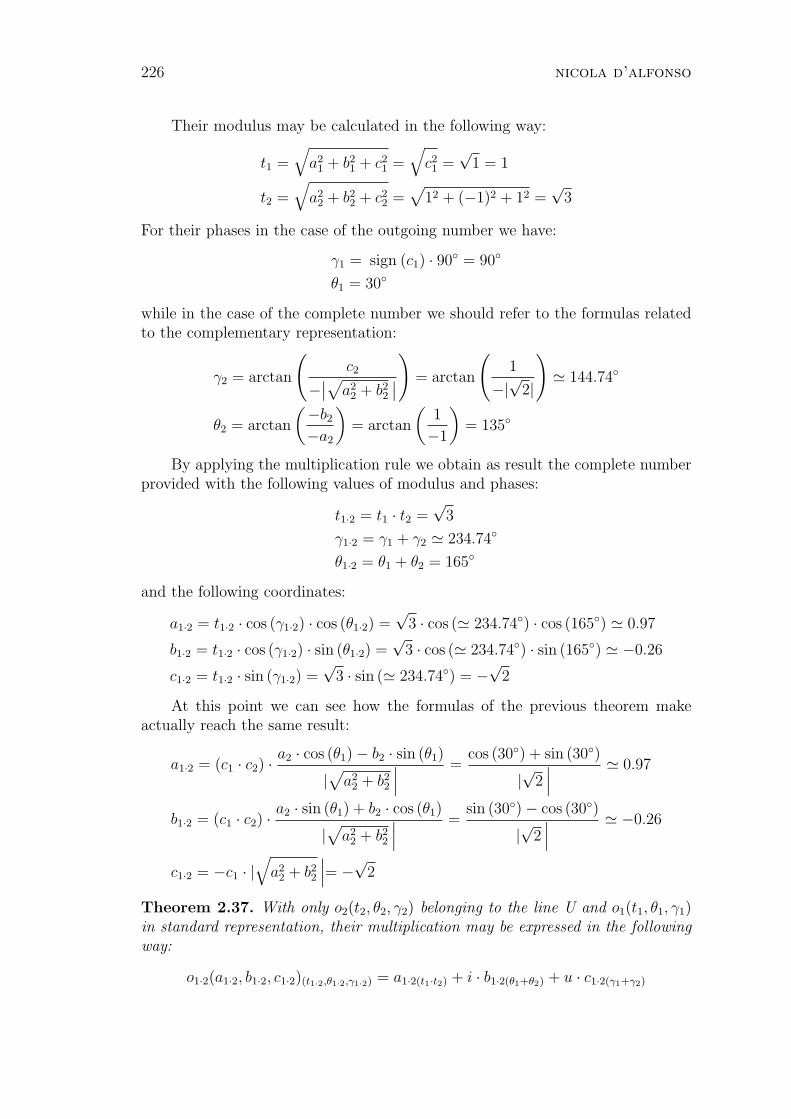
226 nicola d’alfonso
Their modulus may be calculated in the following way:
t1 =√
a21 + b2
1 + c21 =
√c21 =
√1 = 1
t2 =√
a22 + b2
2 + c22 =
√12 + (−1)2 + 12 =
√3
For their phases in the case of the outgoing number we have:
γ1 = sign (c1) · 90 = 90
θ1 = 30
while in the case of the complete number we should refer to the formulas relatedto the complementary representation:
γ2 = arctan
(c2
−∣∣√a2
2 + b22
∣∣
)= arctan
(1
−|√2|
)' 144.74
θ2 = arctan
(−b2
−a2
)= arctan
(1
−1
)= 135
By applying the multiplication rule we obtain as result the complete numberprovided with the following values of modulus and phases:
t1·2 = t1 · t2 =√
3
γ1·2 = γ1 + γ2 ' 234.74
θ1·2 = θ1 + θ2 = 165
and the following coordinates:
a1·2 = t1·2 · cos (γ1·2) · cos (θ1·2) =√
3 · cos (' 234.74) · cos (165) ' 0.97
b1·2 = t1·2 · cos (γ1·2) · sin (θ1·2) =√
3 · cos (' 234.74) · sin (165) ' −0.26
c1·2 = t1·2 · sin (γ1·2) =√
3 · sin (' 234.74) = −√
2
At this point we can see how the formulas of the previous theorem makeactually reach the same result:
a1·2 = (c1 · c2) · a2 · cos (θ1)− b2 · sin (θ1)
|√
a22 + b2
2
∣∣∣=
cos (30) + sin (30)
|√2∣∣∣
' 0.97
b1·2 = (c1 · c2) · a2 · sin (θ1) + b2 · cos (θ1)
|√
a22 + b2
2
∣∣∣=
sin (30)− cos (30)
|√2∣∣∣
' −0.26
c1·2 = −c1 · |√
a22 + b2
2
∣∣∣= −√
2
Theorem 2.37. With only o2(t2, θ2, γ2) belonging to the line U and o1(t1, θ1, γ1)in standard representation, their multiplication may be expressed in the followingway:
o1·2(a1·2, b1·2, c1·2)(t1·2,θ1·2,γ1·2) = a1·2(t1·t2) + i · b1·2(θ1+θ2) + u · c1·2(γ1+γ2)
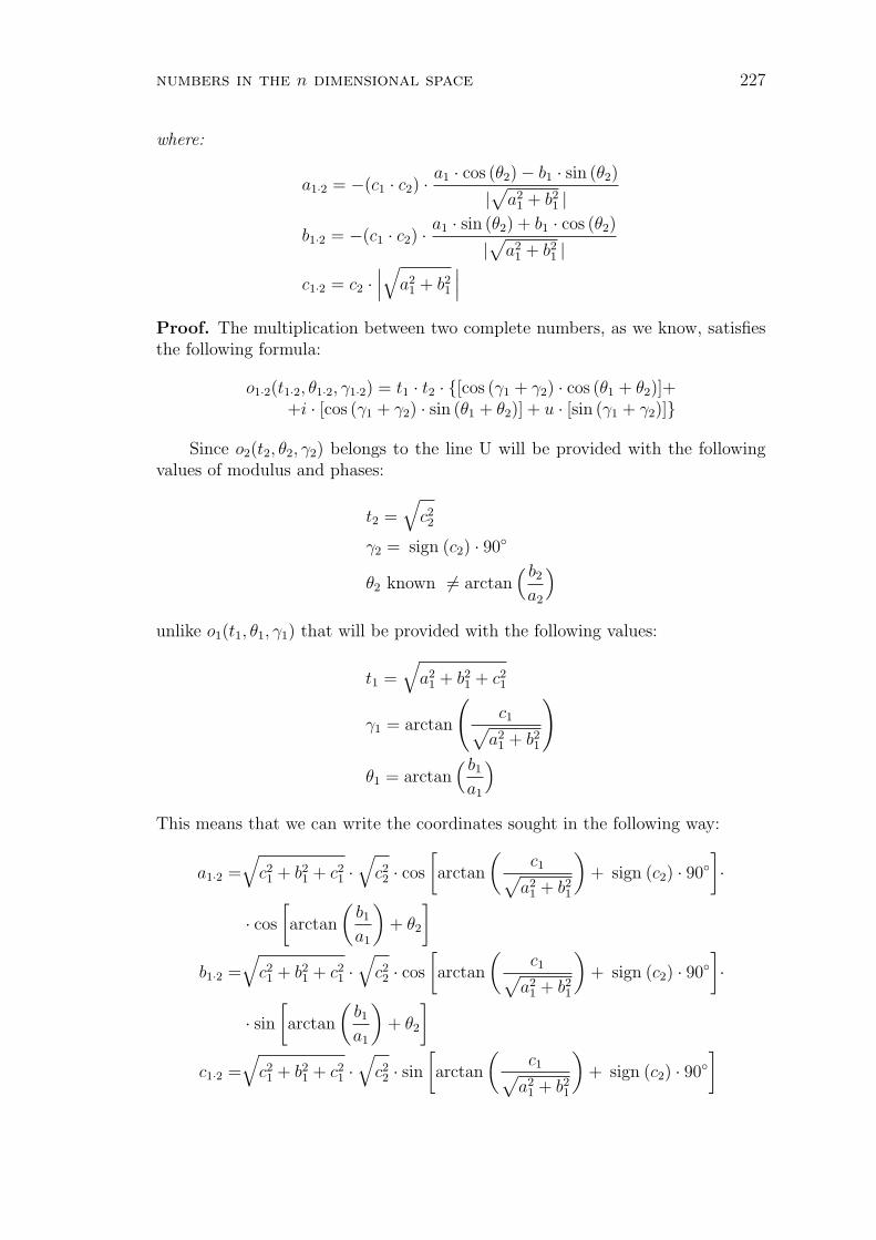
numbers in the n dimensional space 227
where:
a1·2 = −(c1 · c2) · a1 · cos (θ2)− b1 · sin (θ2)
|√
a21 + b2
1 |b1·2 = −(c1 · c2) · a1 · sin (θ2) + b1 · cos (θ2)
|√
a21 + b2
1 |c1·2 = c2 ·
∣∣∣√
a21 + b2
1
∣∣∣
Proof. The multiplication between two complete numbers, as we know, satisfiesthe following formula:
o1·2(t1·2, θ1·2, γ1·2) = t1 · t2 · [cos (γ1 + γ2) · cos (θ1 + θ2)]++i · [cos (γ1 + γ2) · sin (θ1 + θ2)] + u · [sin (γ1 + γ2)]
Since o2(t2, θ2, γ2) belongs to the line U will be provided with the followingvalues of modulus and phases:
t2 =√
c22
γ2 = sign (c2) · 90
θ2 known 6= arctan( b2
a2
)
unlike o1(t1, θ1, γ1) that will be provided with the following values:
t1 =√
a21 + b2
1 + c21
γ1 = arctan
(c1√
a21 + b2
1
)
θ1 = arctan( b1
a1
)
This means that we can write the coordinates sought in the following way:
a1·2 =√
c21 + b2
1 + c21 ·
√c22 · cos
[arctan
(c1√
a21 + b2
1
)+ sign (c2) · 90
]·
· cos
[arctan
(b1
a1
)+ θ2
]
b1·2 =√
c21 + b2
1 + c21 ·
√c22 · cos
[arctan
(c1√
a21 + b2
1
)+ sign (c2) · 90
]·
· sin[arctan
(b1
a1
)+ θ2
]
c1·2 =√
c21 + b2
1 + c21 ·
√c22 · sin
[arctan
(c1√
a21 + b2
1
)+ sign (c2) · 90
]
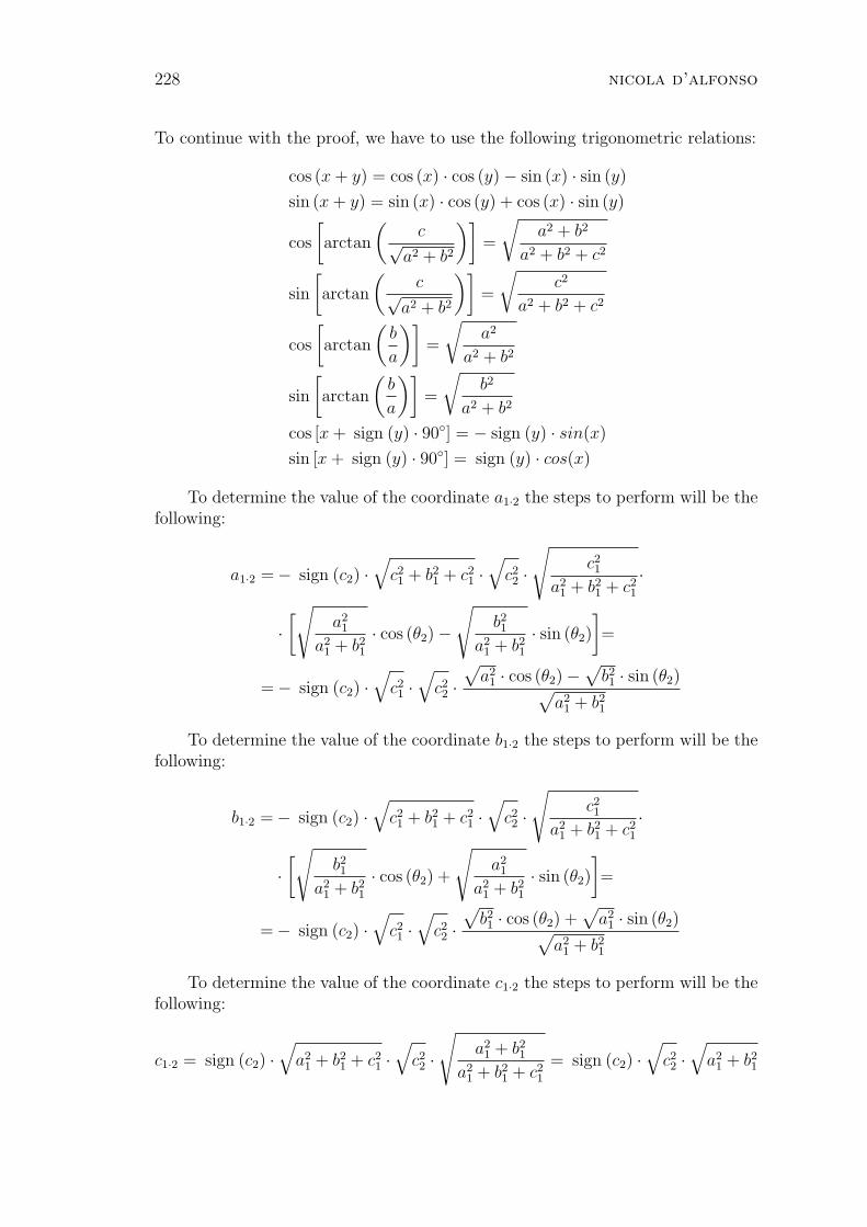
228 nicola d’alfonso
To continue with the proof, we have to use the following trigonometric relations:
cos (x + y) = cos (x) · cos (y)− sin (x) · sin (y)
sin (x + y) = sin (x) · cos (y) + cos (x) · sin (y)
cos
[arctan
(c√
a2 + b2
)]=
√a2 + b2
a2 + b2 + c2
sin
[arctan
(c√
a2 + b2
)]=
√c2
a2 + b2 + c2
cos
[arctan
(b
a
)]=
√a2
a2 + b2
sin
[arctan
(b
a
)]=
√b2
a2 + b2
cos [x + sign (y) · 90] = − sign (y) · sin(x)
sin [x + sign (y) · 90] = sign (y) · cos(x)
To determine the value of the coordinate a1·2 the steps to perform will be thefollowing:
a1·2 =− sign (c2) ·√
c21 + b2
1 + c21 ·
√c22 ·
√c21
a21 + b2
1 + c21
·
·[√
a21
a21 + b2
1
· cos (θ2)−√
b21
a21 + b2
1
· sin (θ2)
]=
=− sign (c2) ·√
c21 ·
√c22 ·
√a2
1 · cos (θ2)−√
b21 · sin (θ2)√
a21 + b2
1
To determine the value of the coordinate b1·2 the steps to perform will be thefollowing:
b1·2 =− sign (c2) ·√
c21 + b2
1 + c21 ·
√c22 ·
√c21
a21 + b2
1 + c21
·
·[√
b21
a21 + b2
1
· cos (θ2) +
√a2
1
a21 + b2
1
· sin (θ2)
]=
=− sign (c2) ·√
c21 ·
√c22 ·
√b21 · cos (θ2) +
√a2
1 · sin (θ2)√a2
1 + b21
To determine the value of the coordinate c1·2 the steps to perform will be thefollowing:
c1·2 = sign (c2) ·√
a21 + b2
1 + c21 ·
√c22 ·
√a2
1 + b21
a21 + b2
1 + c21
= sign (c2) ·√
c22 ·
√a2
1 + b21
numbers in the n dimensional space 229
These relations are valid in general, in the precise sense that they are also ableto include cases where the coefficients a1,b1,c1 are zero (provided that o1(a1, b1, c1)remains in the context of the complete numbers not belonging in the line U).
Wanting to find relations that satisfy the multiplication rule as a function ofthe effective coordinates of the complete numbers involved, we must adopt for thecoefficients a,b,c the convention
√x2 = x, with the exception of c2 for which we
should adopt the convention√
x2 = |x|. The reason is simple because if we adoptfor c2 the usual convention, we will have:
sign (c2) ·√
c22 = |c2|
and therefore a result of the multiplication that depends on the modulus of thecoordinate c2. While adopting
√x2 = |x| we will have:
sign (c2) ·√
c22 = c2
and therefore a result of the multiplication that depends on the effective value ofthis coordinate.
The relations obtained will be the following:
a1·2 = −(c1 · c2) · a1 · cos (θ2)− b1 · sin (θ2)√a2
1 + b21
b1·2 = −(c1 · c2) · a1 · sin (θ2) + b1 · cos (θ2)√a2
1 + b21
c1·2 = c2 ·√
a21 + b2
1
(2.3)
Since the number o1(a1, b1, c1) is in standard representation, as determinedby the theorem 2.11 we must consider the following relation:
√a2
1 + b21 =
∣∣√
a21 + b2
1
∣∣
that combined with those indicated by the formulas (2.3), proving the thesis.
As an example of the theorem just proved, suppose you have to multiply thecomplete number in standard representation provided with coordinates: a1 = 1,b1 = −1, c1 = 1 by an outgoing numbers of coordinate: c2 = 1 and phase θ2 = 30.
Their modulus may be calculated in the following way:
t1 =√
a21 + b2
1 + c21 =
√12 + (−1)2 + 12 =
√3
t2 =√
a22 + b2
2 + c22 =
√c22 =
√1 = 1
For their phases in the case of the outgoing number we have:
γ2 = sign (c2) · 90 = 90
θ2 = 30
230 nicola d’alfonso
while in the case of the complete number we should refer to the formulas relatedto the standard representation:
γ1 = arctan
(c1∣∣√a21 + b2
1
∣∣
)= arctan
(1
|√2|
)' 35.26
θ1 = arctan
(b1
a1
)= arctan
(−1
1
)= −45
By applying the multiplication rule we obtain as result the complete numberprovided with the following values of modulus and phases:
t1·2 = t1 · t2 =√
3
γ1·2 = γ1 + γ2 ' 125.26
θ1·2 = θ1 + θ2 = −15
and the following coordinates:
a1·2 = t1·2 · cos (γ1·2) · cos (θ1·2) =√
3 · cos (' 125.26) · cos (−15) ' −0.97
b1·2 = t1·2 · cos (γ1·2) · sin (θ1·2) =√
3 · cos (' 125.26) · sin (−15) ' 0.26
c1·2 = t1·2 · sin (γ1·2) =√
3 · sin (' 125.26) =√
2
At this point we can see how the formulas of the previous theorem makeactually reach the same result:
a1·2 = −(c1 · c2) · a1 · cos (θ2)− b1 · sin (θ2)|√
a21 + b2
1 |= −cos (30) + sin (30)
|√2 | ' −0.97
b1·2 = −(c1 · c2) · a1 · sin (θ2) + b1 · cos (θ2)|√
a21 + b2
1 |= −sin (30)− cos (30)
|√2 | ' 0.26
c1·2 = c2 ·∣∣∣√
a21 + b2
1
∣∣∣=√
2
Theorem 2.38. With only o2(t2, θ2, γ2) belonging to the line U and o1(t1, θ1, γ1)in complementary representation, their multiplication may be expressed in the fol-lowing way:
o1·2(a1·2, b1·2, c1·2)(t1·2,θ1·2,γ1·2) = a1·2(t1·t2) + i · b1·2(θ1+θ2) + u · c1·2(γ1+γ2)
where
a1·2 = (c1 · c2) · a1 · cos (θ2)− b1 · sin (θ2)
|√
a21 + b2
1 |b1·2 = (c1 · c2) · a1 · sin (θ2) + b1 · cos (θ2)
|√
a21 + b2
1 |c1·2 = −c2 ·
∣∣∣√
a21 + b2
1
∣∣∣
numbers in the n dimensional space 231
Proof. Since the number o1(a1, b1, c1) is in complementary representation, asdetermined by the theorem 2.15 we must consider the following relation:
√a2
1 + b21 = −
∣∣√
a21 + b2
1
∣∣
that combined with those indicated by the formulas (2.3), proving the thesis.
As an example of the theorem just proved, suppose you have to multiplya complete number in complementary representation provided with coordinates:a2 = 1, b2 = −1, c2 = 1 by the outgoing numbers of coordinate: c1 = 1 and phaseθ1 = 30.
Their modulus may be calculated in the following way:
t1 =√
a21 + b2
1 + c21 =
√12 + (−1)2 + 12 =
√3
t2 =√
a22 + b2
2 + c22 =
√c22 =
√1 = 1
For their phases in the case of the outgoing number we have:
γ2 = sign (c2) · 90 = 90
θ2 = 30
while in the case of the complete number we should refer to the formulas relatedto the complementary representation:
γ2 = arctan
(c1
−∣∣√a2
1 + b21
∣∣
)= arctan
(1
−|√2|
)' 144.74
θ2 = arctan
(−b1
−a1
)= arctan
(1
−1
)= 135
By applying the multiplication rule we obtain as result the complete numberprovided with the following values of modulus and phases:
t1·2 = t1 · t2 =√
3
γ1·2 = γ1 + γ2 ' 234.74
θ1·2 = θ1 + θ2 = 165
and the following coordinates:
a1·2 = t1·2 · cos (γ1·2) · cos (θ1·2) =√
3 · cos (' 234.74) · cos (165) ' 0.97
b1·2 = t1·2 · cos (γ1·2) · sin (θ1·2) =√
3 · cos (' 234.74) · sin (165) ' −0.26
c1·2 = t1·2 · sin (γ1·2) =√
3 · sin (' 234.74) = −√
2

232 nicola d’alfonso
At this point we can see how the formulas of the previous theorem makeactually reach the same result:
a1·2 = (c1 · c2) · a1 · cos (θ2)− b1 · sin (θ2)
|√
a21 + b2
1 |=
cos (30) + sin (30)
|√2 | ' 0.97
b1·2 = (c1 · c2) · a1 · sin (θ2) + b1 · cos (θ2)
|√
a21 + b2
1 |=
sin (30)− cos (30)
|√2 | ' −0.26
c1·2 = −c2 ·∣∣∣√
a21 + b2
1
∣∣∣= −√
2
Theorem 2.39. With o1(t1, θ1, γ1) and o2(t2, θ2, γ2) both belonging to the line U,their multiplication may be expressed in the following way:
o1·2(a1·2, b1·2, c1·2)(t1·2,θ1·2,γ1·2) = a1·2(t1·t2) + i · b1·2(θ1+θ2) + u · c1·2(γ1+γ2)
where
a1·2 = −(c1 · c2) · cos (θ1 + θ2)
b1·2 = −(c1 · c2) · sin (θ1 + θ2)
c1·2 = 0
Proof. The multiplication between two complete numbers, as we know, satisfiesthe following formula:
o1·2(t1·2, θ1·2, γ1·2) = t1 · t2 · [cos (γ1 + γ2) · cos (θ1 + θ2)]+
+ i · [cos (γ1 + γ2) · sin (θ1 + θ2)] + u · [sin (γ1 + γ2)]Since o1(t1, θ1, γ1) and o2(t2, θ2, γ2) belong to the line U will be provided with
the following values of modulus and phases:
t1 =√
c21
t2 =√
c22
γ1 = sign (c1) · 90
γ2 = sign (c2) · 90
θ1 known 6= arctan( b1
a1
)
θ2 known 6= arctan( b2
a2
)
This means that we can write the coordinates sought in the following way:
a1·2 =√
c21 ·
√c22 · cos [ sign (c1) · 90 + sign (c2) · 90] · cos (θ1 + θ2)
b1·2 =√
c21 ·
√c22 · cos [ sign (c1) · 90 + sign (c2) · 90] · sin (θ1 + θ2)
c1·2 =√
c21 ·
√c22 · sin [ sign (c1) · 90 + sign (c2) · 90]

numbers in the n dimensional space 233
Considering that when c1 and c2 have the same sign we obtained:
cos [ sign (c1) · 90 + sign (c2) · 90] = cos (±180) = −1 = − sign (c1) · sign (c2)sin [ sign (c1) · 90 + sign (c2) · 90] = sin (±180) = 0
and that when they have the opposite sign we obtained:
cos [ sign (c1) · 90 + sign (c2) · 90] = cos (±0) = 1 = − sign (c1) · sign (c2)sin [ sign (c1) · 90 + sign (c2) · 90] = sin (±0) = 0
we can write:
a1·2 = − sign (c1) · sign (c2) ·√
c21 ·
√c22 · cos (θ1 + θ2)
b1·2 = − sign (c1) · sign (c2) ·√
c21 ·
√c22 · sin (θ1 + θ2)
c1·2 = 0
Wanting to find relations that satisfy the multiplication rule as a function ofthe effective coordinates of the complete numbers involved, we must adopt for thecoefficients c1,c2 the convention
√x2 = |x|. In fact in this way we obtain:
sign (c1) ·√
c21 = c1
sign (c2) ·√
c22 = c2
and therefore a result of the multiplication that depends on the effective value ofthis coordinate. The relation that we obtain following these conventions provesthe thesis.
As an example of the theorem just proved, suppose you have to multiply theoutgoing numbers of coordinate: c1 = 1 and phase θ1 = 30 by the outgoingnumber of coordinate: c2 = 1 and phase θ2 = 30.
Their modulus may be calculated in the following way:
t1 =√
a21 + b2
1 + c21 =
√c21 =
√1 = 1
t2 =√
a22 + b2
2 + c22 =
√c22 =
√1 = 1
For their phases we have:
γ1 = sign (c1) · 90 = 90
γ2 = sign (c2) · 90 = 90
θ1 = 30
θ2 = 30
By applying the multiplication rule we obtain as result the complete numberprovided with the following values of modulus and phases:
t1·2 = t1 · t2 = 1
γ1·2 = γ1 + γ2 = 180
θ1·2 = θ1 + θ2 = 60
234 nicola d’alfonso
and the following coordinates:
a1·2 = t1·2 · cos (γ1·2) · cos (θ1·2) = 1 · cos (180) · cos (60) = −1
2
b1·2 = t1·2 · cos (γ1·2) · sin (θ1·2) = 1 · cos (180) · sin (60) = −√
3
2c1·2 = t1·2 · sin (γ1·2) = 1 · sin (180) = 0
At this point we can see how the formulas of the previous theorem makeactually reach the same result:
a1·2 = −(c1 · c2) · cos (θ1 + θ2) = − cos (60) = −1
2
b1·2 = −(c1 · c2) · sin (θ1 + θ2) = − sin (60) = −√
3
2c1·2 = 0
Theorem 2.40. For the operation of multiplication is defined null the completenumber 0, namely for:
o2(t2, θ2, γ2) = 0
we have:
o1(t1, θ1, γ1) · o2(t2, θ2, γ2) = 0
Proof. t1,θ1,γ1,t2,θ2,γ2 being real numbers, we can write:
t1·2 = t1 · t2 = t1 · 0 = 0
θ1·2 = θ1 + θ2 = θ1 + indeterminate = indeterminate
γ1·2 = γ1 + γ2 = γ1 + indeterminate = indeterminate
proving the thesis.
Theorem 2.41. For the operation of multiplication is defined neuter the completenumber 1(S), namely for:
o2(a2, b2, c2)(S) = 1(S)
we have:
o1(a1, b1, c1)(t1,θ1,γ1) · o2(a2, b2, c2)(S) = o1(a1, b1, c1)(t1,θ1,γ1)
Proof. t1,θ1,γ1,t2,θ2,γ2 being real numbers, we can write:
t1·2 = t1 · t2 = t1 · 1 = t1
θ1·2 = θ1 + θ2 = θ1 + 0 = θ1
γ1·2 = γ1 + γ2 = γ1 + 0 = γ1
proving the thesis.

numbers in the n dimensional space 235
Theorem 2.42. For the operation of multiplication is defined inverse the completenumber that identifies the inverse position with respect the origin, namely for:
o2(t2, θ2, γ2) = o2(1
t1,−θ1,−γ1)
we have:o1(t1, θ1, γ1) · o2(t2, θ2, γ2) = 1(S)
Proof. t1,θ1,γ1,t2,θ2,γ2 being real numbers, we can write:
t1·2 = t1 · t2 = t1 · 1
t1= 1
θ1·2 = θ1 + θ2 = θ1 − θ1 = 0
γ1·2 = γ1 + γ2 = γ1 − γ1 = 0
proving the thesis.
Theorem 2.43. For the operation of multiplication is valid the commutative pro-perty, namely:
o1(t1, θ1, γ1) · o2(t2, θ2, γ2) = o2(t2, θ2, γ2) · o1(t1, θ1, γ1)
Proof. t1,θ1,γ1,t2,θ2,γ2 being real numbers, we can write:
t1·2 = t1 · t2θ1·2 = θ1 + θ2
γ1·2 = γ1 + γ2
t2·1 = t2 · t1 = t1 · t2θ2·1 = θ2 + θ1 = θ1 + θ2
γ2·1 = γ2 + γ1 = γ1 + γ2
proving the thesis.
Theorem 2.44. For the operation of multiplication are valid the associative anddissociative properties, namely for:
o2(t2, θ2, γ2) = o3(t3, θ3, γ3) + o4(t4, θ4, γ4)
we have:
[o1(t1, θ1, γ1) · o3(t3, θ3, γ3)] · o4(t4, θ4, γ4) = o1(t1, θ1, γ1) · o2(t2, θ2, γ2)
o1(t1, θ1, γ1) · o2(t2, θ2, γ2) = [o1(t1, θ1, γ1) · o3(t3, θ3, γ3)] · o4(t4, θ4, γ4)
Proof. t1,θ1,γ1,t2,θ2,γ2,t3,θ3,γ3,t4,θ4,γ4 being real numbers, we can write:
t(1·3)·4 = (t1 · t3) · t4 = t1 · (t3 · t4)θ(1·3)·4 = (θ1 + θ3) + θ4 = θ1 + (θ3 + θ4)
γ(1·3)·4 = (γ1 + γ3) + γ4 = γ1 + (γ3 + γ4)

236 nicola d’alfonso
t1·2 = t1 · t2 = t1 · (t3 · t4)θ1·2 = θ1 + θ2 = θ1 + (θ3 + θ4)
γ1·2 = γ1 + γ2 = γ1 + (γ3 + γ4)
proving the thesis.
Theorem 2.45. It is not valid the distributive property of multiplication overaddition, namely for:
o2(t2, θ2, γ2) = o3(t3, θ3, γ3) + o4(t4, θ4, γ4)
we have:
o1(t1, θ1, γ1) · o2(t2, θ2, γ2) 6= [o1(t1, θ1, γ1) · o3(t3, θ3, γ3)] + [o1(t1, θ1, γ1) · o4(t4, θ4, γ4)]
Proof. Referring to the situation described by theorem 2.31 and considering thata1,b1,c1,a2,b2,c2, a3,b3,c3,a4,b4,c4 are real numbers, we can write:
c1·2 = c1 ·∣∣∣√
(a22 + b2
2)∣∣∣+c2 ·
∣∣∣√
(a21 + b2
1)∣∣∣
c(1·3)+(1·4) =[c1 ·
∣∣∣√
(a23 + b2
3)∣∣∣+c3 ·
∣∣∣√
(a21 + b2
1)∣∣∣]
+[c1 ·
∣∣∣√
(a24 + b2
4)∣∣∣+c4 ·
∣∣∣√
(a21 + b2
1)∣∣∣]
= c1 ·[∣∣∣
√(a2
3 + b23)
∣∣∣+∣∣∣√
(a24 + b2
4)∣∣∣]+(c3 + c4) ·
∣∣∣√
(a21 + b2
1)∣∣∣
= c1 ·[∣∣∣
√(a2
3 + b23)
∣∣∣+∣∣∣√
(a24 + b2
4)∣∣∣]+c2 ·
∣∣∣√
(a21 + b2
1)∣∣∣ 6= c1·2
proving the thesis.
Theorem 2.46. It is not valid the distributive property of multiplication oversubtraction, namely for:
o2(t2, θ2, γ2) = o3(t3, θ3, γ3)− o4(t4, θ4, γ4)
we have:
o1(t1, θ1, γ1) · o2(t2, θ2, γ2) 6= [o1(t1, θ1, γ1) · o3(t3, θ3, γ3)]− [o1(t1, θ1, γ1) · o4(t4, θ4, γ4)]
Proof. Referring to the situation described by theorem 2.31 and considering thata1,b1,c1,a2,b2,c2, a3,b3,c3,a4,b4,c4 are real numbers, we can write:
c1·2 = c1 ·∣∣∣√
(a22 + b2
2)∣∣∣+c2 ·
∣∣∣√
(a21 + b2
1)∣∣∣
c(1·3)−(1·4) =[c1 ·
∣∣∣√
(a23 + b2
3)∣∣∣+c3 ·
∣∣∣√
(a21 + b2
1)∣∣∣]
−[c1 ·
∣∣∣√
(a24 + b2
4)∣∣∣+c4 ·
∣∣∣√
(a21 + b2
1)∣∣∣]
= c1 ·[∣∣∣
√(a2
3 + b23)
∣∣∣−∣∣∣√
(a24 + b2
4)∣∣∣]+(c3 − c4) ·
∣∣∣√
(a21 + b2
1)∣∣∣
= c1 ·[∣∣∣
√(a2
3 + b23)
∣∣∣−∣∣∣√
(a24 + b2
4)∣∣∣]+c2 ·
∣∣∣√
(a21 + b2
1)∣∣∣ 6= c1·2
proving the thesis.
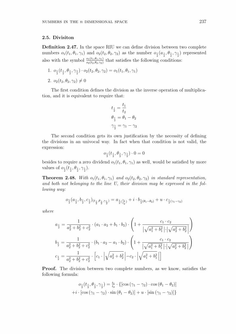
numbers in the n dimensional space 237
2.5. Divisiton
Definition 2.47. In the space RIU we can define division between two completenumbers o1(t1, θ1, γ1) and o2(t2, θ2, γ2) as the number o 1
2(a 1
2, θ 1
2, γ 1
2) represented
also with the symbol o1(t1,θ1,γ1)o2(t2,θ2,γ2)
that satisfies the following conditions:
1. o 12(t 1
2, θ 1
2, γ 1
2) · o2(t2, θ2, γ2) = o1(t1, θ1, γ1)
2. o2(t2, θ2, γ2) 6= 0
The first condition defines the division as the inverse operation of multiplica-tion, and it is equivalent to require that:
t 12
=t1t2
θ 12
= θ1 − θ2
γ 12
= γ1 − γ2
The second condition gets its own justification by the necessity of definingthe divisions in an univocal way. In fact when that condition is not valid, theexpression:
o 12(t 1
2, θ 1
2, γ 1
2) · 0 = 0
besides to require a zero dividend o1(t1, θ1, γ1) as well, would be satisfied by morevalues of o 1
2(t 1
2, θ 1
2, γ 1
2).
Theorem 2.48. With o1(t1, θ1, γ1) and o2(t2, θ2, γ2) in standard representation,and both not belonging to the line U, their division may be expressed in the fol-lowing way:
o 12(a 1
2, b 1
2, c 1
2)(t 1
2,θ 1
2,γ 1
2) = a 1
2(
t1t2
) + i · b 12(θ1−θ2) + u · c 1
2(γ1−γ2)
where
a 12
=1
a22 + b2
2 + c22
· (a1 · a2 + b1 · b2) ·(
1 +c1 · c2∣∣√a2
1 + b21
∣∣·∣∣√a2
2 + b22
∣∣∣
)
b 12
=1
a22 + b2
2 + c22
· (b1 · a2 − a1 · b2) ·(
1 +c1 · c2∣∣√a2
1 + b21
∣∣·∣∣√a2
2 + b22
∣∣
)
c 12
=1
a22 + b2
2 + c22
·[c1 ·
∣∣∣√
a22 + b2
2
∣∣∣−c2 ·∣∣∣√
a21 + b2
1
∣∣∣]
Proof. The division between two complete numbers, as we know, satisfies thefollowing formula:
o 12(t 1
2, θ 1
2, γ 1
2) = t1
t2· [cos (γ1 − γ2) · cos (θ1 − θ2)]
+i · [cos (γ1 − γ2) · sin (θ1 − θ2)] + u · [sin (γ1 − γ2)]
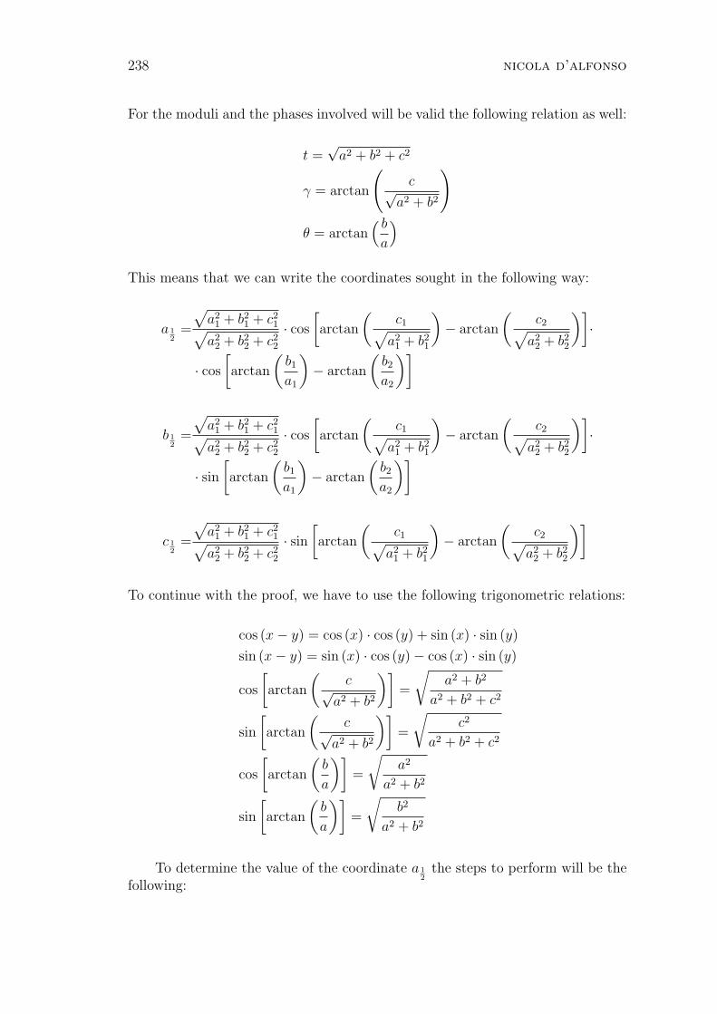
238 nicola d’alfonso
For the moduli and the phases involved will be valid the following relation as well:
t =√
a2 + b2 + c2
γ = arctan
(c√
a2 + b2
)
θ = arctan( b
a
)
This means that we can write the coordinates sought in the following way:
a 12
=
√a2
1 + b21 + c2
1√a2
2 + b22 + c2
2
· cos
[arctan
(c1√
a21 + b2
1
)− arctan
(c2√
a22 + b2
2
)]·
· cos
[arctan
(b1
a1
)− arctan
(b2
a2
)]
b 12
=
√a2
1 + b21 + c2
1√a2
2 + b22 + c2
2
· cos
[arctan
(c1√
a21 + b2
1
)− arctan
(c2√
a22 + b2
2
)]·
· sin[arctan
(b1
a1
)− arctan
(b2
a2
)]
c 12
=
√a2
1 + b21 + c2
1√a2
2 + b22 + c2
2
· sin[arctan
(c1√
a21 + b2
1
)− arctan
(c2√
a22 + b2
2
)]
To continue with the proof, we have to use the following trigonometric relations:
cos (x− y) = cos (x) · cos (y) + sin (x) · sin (y)
sin (x− y) = sin (x) · cos (y)− cos (x) · sin (y)
cos
[arctan
(c√
a2 + b2
)]=
√a2 + b2
a2 + b2 + c2
sin
[arctan
(c√
a2 + b2
)]=
√c2
a2 + b2 + c2
cos
[arctan
(b
a
)]=
√a2
a2 + b2
sin
[arctan
(b
a
)]=
√b2
a2 + b2
To determine the value of the coordinate a 12
the steps to perform will be thefollowing:
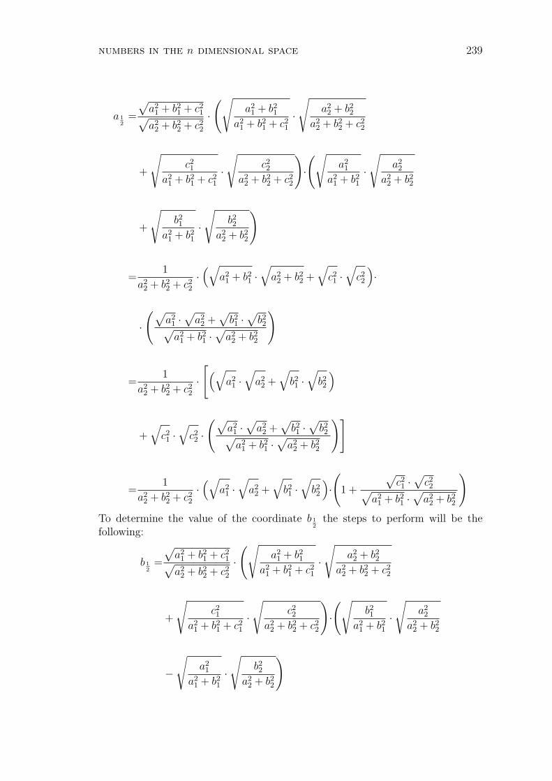
numbers in the n dimensional space 239
a 12
=
√a2
1 + b21 + c2
1√a2
2 + b22 + c2
2
·(√
a21 + b2
1
a21 + b2
1 + c21
·√
a22 + b2
2
a22 + b2
2 + c22
+
√c21
a21 + b2
1 + c21
·√
c22
a22 + b2
2 + c22
)·(√
a21
a21 + b2
1
·√
a22
a22 + b2
2
+
√b21
a21 + b2
1
·√
b22
a22 + b2
2
)
=1
a22 + b2
2 + c22
·(√
a21 + b2
1 ·√
a22 + b2
2 +√
c21 ·
√c22
)·
·(√
a21 ·
√a2
2 +√
b21 ·
√b22√
a21 + b2
1 ·√
a22 + b2
2
)
=1
a22 + b2
2 + c22
·[(√
a21 ·
√a2
2 +√
b21 ·
√b22
)
+√
c21 ·
√c22 ·
(√a2
1 ·√
a22 +
√b21 ·
√b22√
a21 + b2
1 ·√
a22 + b2
2
)]
=1
a22 + b2
2 + c22
·(√
a21 ·
√a2
2 +√
b21 ·
√b22
)·(
1 +
√c21 ·
√c22√
a21 + b2
1 ·√
a22 + b2
2
)
To determine the value of the coordinate b 12
the steps to perform will be thefollowing:
b 12
=
√a2
1 + b21 + c2
1√a2
2 + b22 + c2
2
·(√
a21 + b2
1
a21 + b2
1 + c21
·√
a22 + b2
2
a22 + b2
2 + c22
+
√c21
a21 + b2
1 + c21
·√
c22
a22 + b2
2 + c22
)·(√
b21
a21 + b2
1
·√
a22
a22 + b2
2
−√
a21
a21 + b2
1
·√
b22
a22 + b2
2
)
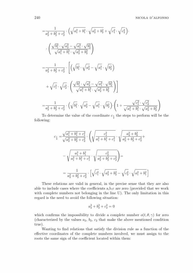
240 nicola d’alfonso
=1
a22 + b2
2 + c22
·(√
a21 + b2
1 ·√
a22 + b2
2 +√
c21 ·
√c22
)·
·(√
b21 ·
√a2
2 −√
a21 ·
√b22√
a21 + b2
1 ·√
a22 + b2
2
)
=1
a22 + b2
2 + c22
·[(√
b21 ·
√a2
2 −√
a21 ·
√b22
)
+√
c21 ·
√c22 ·
(√b21 ·
√a2
2 −√
a21 ·
√b22√
a21 + b2
1 ·√
a22 + b2
2
)]
=1
a22 + b2
2 + c22
·(√
b21 ·
√a2
2 −√
a21 ·
√b22
)·(
1 +
√c21 ·
√c22√
a21 + b2
1 ·√
a22 + b2
2
)
To determine the value of the coordinate c 12
the steps to perform will be thefollowing:
c 12
=
√a2
1 + b21 + c2
1√a2
2 + b22 + c2
2
·(√
c21
a21 + b2
1 + c21
·√
a22 + b2
2
a22 + b2
2 + c22
+
−√
a21 + b2
1
a21 + b2
1 + c21
·√
c22
a22 + b2
2 + c22
)=
=1
a22 + b2
2 + c22
·[√
c21 ·
√a2
2 + b22 −
√c22 ·
√a2
1 + b21
]
These relations are valid in general, in the precise sense that they are alsoable to include cases where the coefficients a,b,c are zero (provided that we workwith complete numbers not belonging in the line U). The only limitation in thisregard is the need to avoid the following situation:
a22 + b2
2 + c22 = 0
which confirms the impossibility to divide a complete number o(t, θ, γ) for zero(characterized by the values a2, b2, c2 that make the above mentioned conditiontrue).
Wanting to find relations that satisfy the division rule as a function of theeffective coordinates of the complete numbers involved, we must assign to theroots the same sign of the coefficient located within them:
numbers in the n dimensional space 241
√a2 = a√b2 = b√c2 = c
The relations obtained will be the following:
a 12
=1
a22 + b2
2 + c22
· (a1 · a2 + b1 · b2) ·(
1 +c1 · c2√
a21 + b2
1 ·√
a22 + b2
2
)
b 12
=1
a22 + b2
2 + c22
· (b1 · a2 − a1 · b2) ·(
1 +c1 · c2√
a21 + b2
1 ·√
a22 + b2
2
)
c 12
=1
a22 + b2
2 + c22
·[c1 ·
√a2
2 + b22 + c2 ·
√a2
1 + b21
]
(2.4)
Since the complete numbers involved are in standard representation, as de-termined by the theorem 2.11 we must consider the following relations:
√a2
1 + b21 =
∣∣√
a21 + b2
1
∣∣√
a22 + b2
2 =∣∣√
a22 + b2
2
∣∣
that combined with those indicated by the formulas (2.4), proving the thesis.
As an example of the theorem just proved, suppose you have to divide thecomplete numbers in standard representation provided with coordinates: a1 =a2 = b1 = b2 = c1 = c2 = 1.
Their modulus may be calculated in the following way:
t1 = t2 =√
a21 + b2
1 + c21 =
√a2
2 + b22 + c2
2 =√
12 + 12 + 12 =√
3
For their phases we should refer to the formulas related to the standard represen-tation:
γ1 = γ2 = arctan
(c1∣∣√a21 + b2
1
∣∣
)= arctan
(c2∣∣√a22 + b2
2
∣∣
)=
= arctan
(1
|√2|
)' 35.26
θ1 = θ2 = arctan
(b1
a1
)= arctan
(b2
a2
)= arctan
(1
1
)= 45
By applying the division rule we obtain as result the complete number pro-vided with the following values of modulus and phases:
t 12
=t1t2
= 1
γ 12
= γ1 − γ2 = 0
θ 12
= θ1 − θ2 = 0
242 nicola d’alfonso
and the following coordinates:
a 12
= t 12· cos (γ 1
2) · cos (θ 1
2) = 1 · cos (0) · cos (0) = 1
b 12
= t 12· cos (γ 1
2) · sin (θ 1
2) = 1 · cos (0) · sin (0) = 0
c 12
= t 12· sin (γ 1
2) = 1 · sin (0) = 0
At this point we can see how the formulas of the previous theorem makeactually reach the same result:
a 12
=1
a22 + b2
2 + c22
· (a1 · a2 + b1 · b2) ·(
1 +c1 · c2∣∣√a2
1 + b21
∣∣·∣∣√a2
2 + b22
∣∣∣
)=
=1
3· (1 + 1) ·
(1 +
1
2
)= 1
b 12
=1
a22 + b2
2 + c22
· (b1 · a2 − a1 · b2) ·(
1 +c1 · c2∣∣√a2
1 + b21
∣∣·∣∣√a2
2 + b22
∣∣
)=
=1
3· (1− 1) ·
(1 +
1
2
)= 0
c 12
=1
a22 + b2
2 + c22
·[c1 ·
∣∣∣√
a22 + b2
2
∣∣∣−c2 ·∣∣∣√
a21 + b2
1
∣∣∣]=
=1
3· [1 ·
√2− 1 ·
√2] = 0
Theorem 2.49. With o1(t1, θ1, γ1) and o2(t2, θ2, γ2) in complementary represen-tation, and both not belonging to the line U, their division may be expressed in thefollowing way:
o 12(a 1
2, b 1
2, c 1
2)(t 1
2,θ 1
2,γ 1
2) = a 1
2(
t1t2
) + i · b 12(θ1−θ2) + u · c 1
2(γ1−γ2)
where
a 12
=1
a22 + b2
2 + c22
· (a1 · a2 + b1 · b2) ·(
1 +c1 · c2∣∣√a2
1 + b21
∣∣·∣∣√a2
2 + b22
∣∣∣
)
b 12
=1
a22 + b2
2 + c22
· (b1 · a2 − a1 · b2) ·(
1 +c1 · c2∣∣√a2
1 + b21
∣∣·∣∣√a2
2 + b22
∣∣
)
c 12
=1
a22 + b2
2 + c22
·[c2 ·
∣∣∣√
a21 + b2
1
∣∣∣−c1 ·∣∣∣√
a22 + b2
2
∣∣∣]
Proof. Since the complete numbers involved are in complementary representa-tion, as determined by the theorem 2.15 we must consider the following relations:
√a2
1 + b21 = −
∣∣√
a21 + b2
1
∣∣√
a22 + b2
2 = −∣∣√
a22 + b2
2
∣∣
that combined with those indicated by the formulas (2.4), proving the thesis.
numbers in the n dimensional space 243
As an example of the theorem just proved, suppose you have to divide thecomplete numbers in complementary representation provided with coordinates:a1 = a2 = b1 = b2 = c1 = c2 = 1.
Their modulus may be calculated in the following way:
t1 = t2 =√
a21 + b2
1 + c21 =
√a2
2 + b22 + c2
2 =√
12 + 12 + 12 =√
3
For their phases we should refer to the formulas related to the complementaryrepresentation:
γ1 = γ2 = arctan
(c1
−∣∣√a2
1 + b21
∣∣
)= arctan
(c2
−∣∣√a2
2 + b22
∣∣
)=
= arctan
(1
−|√2|
)' 144.73
θ1 = θ2 = arctan
(−b1
−a1
)= arctan
(−b2
−a2
)= arctan
(−1
−1
)= 225
By applying the division rule we obtain as result the complete number pro-vided with the following values of modulus and phases:
t 12
=t1t2
= 1
γ 12
= γ1 − γ2 = 0
θ 12
= θ1 − θ2 = 0
and the following coordinates:
a 12
= t 12· cos (γ 1
2) · cos (θ 1
2) = 1 · cos (0) · cos (0) = 1
b 12
= t 12· cos (γ 1
2) · sin (θ 1
2) = 1 · cos (0) · sin (0) = 0
c 12
= t 12· sin (γ 1
2) = 1 · sin (0) = 0
At this point we can see how the formulas of the previous theorem makeactually reach the same result:
a 12
=1
a22 + b2
2 + c22
· (a1 · a2 + b1 · b2) ·(
1 +c1 · c2∣∣√a2
1 + b21
∣∣·∣∣√a2
2 + b22
∣∣∣
)
=1
3· (1 + 1) ·
(1 +
1
2
)= 1
b 12
=1
a22 + b2
2 + c22
· (b1 · a2 − a1 · b2) ·(
1 +c1 · c2∣∣√a2
1 + b21
∣∣·∣∣√a2
2 + b22
∣∣
)
=1
3· (1− 1) ·
(1 +
1
2
)= 0
c 12
=1
a22 + b2
2 + c22
·[c2 ·
∣∣∣√
a21 + b2
1
∣∣∣−c1 ·∣∣∣√
a22 + b2
2
∣∣∣]
=1
3· [1 ·
√2− 1 ·
√2] = 0
244 nicola d’alfonso
Theorem 2.50. With o1(t1, θ1, γ1) in standard representation and o2(t2, θ2, γ2) incomplementary representation, and both not belonging to the line U, their divisionmay be expressed in the following way:
o 12(a 1
2, b 1
2, c 1
2)(t 1
2,θ 1
2,γ 1
2) = a 1
2(
t1t2
) + i · b 12(θ1−θ2) + u · c 1
2(γ1−γ2)
where
a 12
=1
a22 + b2
2 + c22
· (a1 · a2 + b1 · b2) ·(
1− c1 · c2∣∣√a21 + b2
1
∣∣·∣∣√a2
2 + b22
∣∣∣
)
b 12
=1
a22 + b2
2 + c22
· (b1 · a2 − a1 · b2) ·(
1− c1 · c2∣∣√a21 + b2
1
∣∣·∣∣√a2
2 + b22
∣∣
)
c 12
=1
a22 + b2
2 + c22
·[−c1 ·
∣∣∣√
a22 + b2
2
∣∣∣−c2 ·∣∣∣√
a21 + b2
1
∣∣∣]
Proof. Since the dividend is in standard representation, as determined by thetheorem 2.11 we must consider the following relation:
√a2
1 + b21 =
∣∣√
a21 + b2
1
∣∣
while being the divisor in complementary representation, as determined by thetheorem 2.15 we must consider the following relation:
√a2
2 + b22 = −
∣∣√
a22 + b2
2
∣∣
that combined with those indicated by the formulas (2.4), proving the thesis.
As an example of the theorem just proved, suppose you have to divide thecomplete number in standard representation provided with coordinates a1 = b1 =c1 = 1 by that in complementary representation provided with the same coordi-nates coordinates: a2 = b2 = c2 = 1.
Their modulus may be calculated in the following way:
t1 = t2 =√
a21 + b2
1 + c21 =
√a2
2 + b22 + c2
2 =√
12 + 12 + 12 =√
3
For their phases we should refer to the formulas related to the standard andcomplementary representations:
γ1 = arctan
(c1∣∣√a21 + b2
1
∣∣
)= arctan
(1
|√2|
)' 35.26
γ2 = arctan
(c2
−∣∣√a22 + b2
2
∣∣
)= arctan
(1
−|√2|
)' 144.73
θ1 = arctan
(b1
a1
)= arctan
(1
1
)= 45
θ2 = arctan
(−b2
−a2
)= arctan
(−1
−1
)= 225
numbers in the n dimensional space 245
By applying the division rule we obtain as result the complete number pro-vided with the following values of modulus and phases:
t 12
=t1t2
= 1
γ 12
= γ1 − γ2 ' −109.47
θ 12
= θ1 − θ2 = −180
and the following coordinates:
a 12
= t 12· cos (γ 1
2) · cos (θ 1
2) = 1 · cos (' −109.47) · cos (−180) =
1
3b 1
2= t 1
2· cos (γ 1
2) · sin (θ 1
2) = 1 · cos (' −109.47) · sin (−180) = 0
c 12
= t 12· sin (γ 1
2) = 1 · sin (' −109.47) =
−2 · √2
3At this point we can see how the formulas of the previous theorem make
actually reach the same result:
a 12
=1
a22 + b2
2 + c22
· (a1 · a2 + b1 · b2) ·(
1− c1 · c2∣∣√a21 + b2
1
∣∣·∣∣√a2
2 + b22
∣∣∣
)=
=1
3· (1 + 1) ·
(1− 1
2
)=
1
3
b 12
=1
a22 + b2
2 + c22
· (b1 · a2 − a1 · b2) ·(
1− c1 · c2∣∣√a21 + b2
1
∣∣·∣∣√a2
2 + b22
∣∣
)=
=1
3· (1− 1) ·
(1− 1
2
)= 0
c 12
=1
a22 + b2
2 + c22
·[−c1 ·
∣∣∣√
a22 + b2
2
∣∣∣−c2 ·∣∣∣√
a21 + b2
1
∣∣∣]=
=1
3· [−1 ·
√2− 1 ·
√2] =
−2 · √2
3
Theorem 2.51. With o1(t1, θ1, γ1) in complementary representation and o2(t2, θ2, γ2)in standard representation, and both not belonging to the line U, their division maybe expressed in the following way:
o 12(a 1
2, b 1
2, c 1
2)(t 1
2,θ 1
2,γ 1
2) = a 1
2(
t1t2
) + i · b 12(θ1−θ2) + u · c 1
2(γ1−γ2)
where:
a 12
=1
a22 + b2
2 + c22
· (a1 · a2 + b1 · b2) ·(
1− c1 · c2∣∣√a21 + b2
1
∣∣·∣∣√
a22 + b2
2
∣∣∣
)
b 12
=1
a22 + b2
2 + c22
· (b1 · a2 − a1 · b2) ·(
1− c1 · c2∣∣√a21 + b2
1
∣∣·∣∣√a2
2 + b22
∣∣
)
c 12
=1
a22 + b2
2 + c22
·[c1 ·
∣∣∣√
a22 + b2
2
∣∣∣+c2 ·∣∣∣√
a21 + b2
1
∣∣∣]
246 nicola d’alfonso
Proof. Since the dividend is in complementary representation, as determined bythe theorem 2.15 we must consider the following relation:
√a2
1 + b21 = −
∣∣√
a21 + b2
1
∣∣
while being the divisor in standard representation, as determined by the theorem2.11 we must consider the following relation:
√a2
2 + b22 =
∣∣√
a22 + b2
2
∣∣
that combined with those indicated by the formulas (2.4), proving the thesis.
As an example of the theorem just proved, suppose you have to divide thecomplete number in complementary representation provided with coordinatesa1 = b1 = c1 = 1 by that in standard representation provided with the samecoordinates coordinates: a2 = b2 = c2 = 1.
Their modulus may be calculated in the following way:
t1 = t2 =√
a21 + b2
1 + c21 =
√a2
2 + b22 + c2
2 =√
12 + 12 + 12 =√
3
For their phases we should refer to the formulas related to the complementaryand standard representations:
γ1 = arctan
(c1
−∣∣√a2
1 + b21
∣∣
)= arctan
(1
−|√2|
)' 144.73
γ2 = arctan
(c2∣∣√a22 + b2
2
∣∣
)= arctan
(1
|√2|
)' 35.26
θ1 = arctan
(−b1
−a1
)= arctan
(−1
−1
)= 225
θ2 = arctan
(b2
a2
)= arctan
(1
1
)= 45
By applying the division rule we obtain as result the complete number pro-vided with the following values of modulus and phases:
t 12
=t1t2
= 1
γ 12
= γ1 − γ2 ' 109.47
θ 12
= θ1 − θ2 = 180
and the following coordinates:
a 12
= t 12· cos (γ 1
2) · cos (θ 1
2) = 1 · cos (' 109.47) · cos (180) =
1
3b 1
2= t 1
2· cos (γ 1
2) · sin (θ 1
2) = 1 · cos (' 109.47) · sin (180) = 0
c 12
= t 12· sin (γ 1
2) = 1 · sin (' 109.47) =
2 · √2
3
numbers in the n dimensional space 247
At this point we can see how the formulas of the previous theorem makeactually reach the same result:
a 12
=1
a22 + b2
2 + c22
· (a1 · a2 + b1 · b2) ·(
1− c1 · c2∣∣√a21 + b2
1
∣∣·∣∣√a2
2 + b22
∣∣∣
)
=1
3· (1 + 1) ·
(1− 1
2
)=
1
3
b 12
=1
a22 + b2
2 + c22
· (b1 · a2 − a1 · b2) ·(
1− c1 · c2∣∣√a21 + b2
1
∣∣·∣∣√a2
2 + b22
∣∣
)
=1
3· (1− 1) ·
(1− 1
2
)= 0
c 12
=1
a22 + b2
2 + c22
·[c1 ·
∣∣∣√
a22 + b2
2
∣∣∣+c2 ·∣∣∣√
a21 + b2
1
∣∣∣]
=1
3· [1 ·
√2 + 1 ·
√2] =
2 · √2
3
Theorem 2.52. With only o1(t1, θ1, γ1) belonging to the line U and o2(t2, θ2, γ2)in standard representation, their division may be expressed in the following way:
o 12(a 1
2, b 1
2, c 1
2)(t 1
2,θ 1
2,γ 1
2) = a 1
2(
t1t2
) + i · b 12(θ1−θ2) + u · c 1
2(γ1−γ2)
where:
a 12
=1
a22 + b2
2 + c22
· (c1 · c2) · a2 · cos (θ1) + b2 · sin (θ1)
|√
a22 + b2
2 |b 1
2=
1
a22 + b2
2 + c22
· (c1 · c2) · a2 · sin (θ1)− b2 · cos (θ1)
|√
a22 + b2
2 |c 1
2=
1
a22 + b2
2 + c22
· c1 ·∣∣∣√
a22 + b2
2
∣∣∣
Proof. The division between two complete numbers, as we know, satisfies thefollowing formula:
o 12(t 1
2, θ 1
2, γ 1
2) =
t1t2· [cos (γ1 − γ2) · cos (θ1 − θ2)]
+i · [cos (γ1 − γ2) · sin (θ1 − θ2)] + u · [sin (γ1 − γ2)]Since o1(t1, θ1, γ1) belongs to the line U will be provided with the following
values of modulus and phases:
t1 =√
c21
γ1 = sign (c1) · 90
θ1 known 6= arctan( b1
a1
)
248 nicola d’alfonso
unlike o2(t2, θ2, γ2) that will be provided with the following values:
t2 =√
a22 + b2
2 + c22
γ2 = arctan
(c2√
a22 + b2
2
)
θ2 = arctan( b2
a2
)
This means that we can write the coordinates sought in the following way:
a 12
=
√c21√
a22 + b2
2 + c22
· cos
[sign (c1) · 90 − arctan
(c2√
a22 + b2
2
)]·
· cos
[θ1 − arctan
(b2
a2
)]
b 12
=
√c21√
a22 + b2
2 + c22
· cos
[sign (c1) · 90 − arctan
(c2√
a22 + b2
2
)]·
· sin[θ1 − arctan
(b2
a2
)]
c 12
=
√c21√
a22 + b2
2 + c22
· sin[
sign (c1) · 90 − arctan
(c2√
a22 + b2
2
)]
To continue with the proof, we have to use the following trigonometric relations:
cos (x− y) = cos (x) · cos (y) + sin (x) · sin (y)
sin (x− y) = sin (x) · cos (y)− cos (x) · sin (y)
cos
[arctan
(c√
a2 + b2
)]=
√a2 + b2
a2 + b2 + c2
sin
[arctan
(c√
a2 + b2
)]=
√c2
a2 + b2 + c2
cos
[arctan
(b
a
)]=
√a2
a2 + b2
sin
[arctan
(b
a
)]=
√b2
a2 + b2
cos [ sign (x) · 90 − y] = sign (x) · sin(y)
sin [ sign (x) · 90 − y] = sign (x) · cos(y)
To determine the value of the coordinate a 12
the steps to perform will be thefollowing:
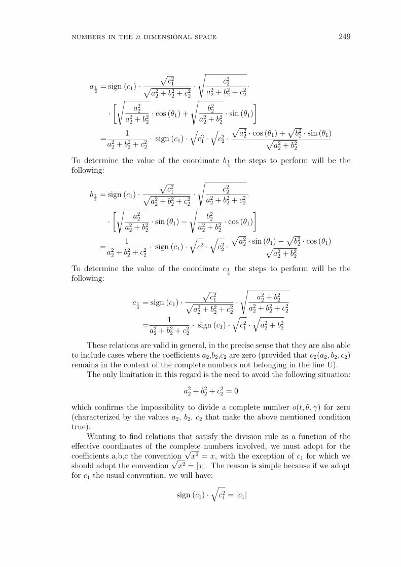
numbers in the n dimensional space 249
a 12
= sign (c1) ·√
c21√
a22 + b2
2 + c22
·√
c22
a22 + b2
2 + c22
·
·[√
a22
a22 + b2
2
· cos (θ1) +
√b22
a22 + b2
2
· sin (θ1)
]
=1
a22 + b2
2 + c22
· sign (c1) ·√
c21 ·
√c22 ·
√a2
2 · cos (θ1) +√
b22 · sin (θ1)√
a22 + b2
2
To determine the value of the coordinate b 12
the steps to perform will be thefollowing:
b 12
= sign (c1) ·√
c21√
a22 + b2
2 + c22
·√
c22
a22 + b2
2 + c22
·
·[√
a22
a22 + b2
2
· sin (θ1)−√
b22
a22 + b2
2
· cos (θ1)
]
=1
a22 + b2
2 + c22
· sign (c1) ·√
c21 ·
√c22 ·
√a2
2 · sin (θ1)−√
b22 · cos (θ1)√
a22 + b2
2
To determine the value of the coordinate c 12
the steps to perform will be thefollowing:
c 12
= sign (c1) ·√
c21√
a22 + b2
2 + c22
·√
a22 + b2
2
a22 + b2
2 + c22
=1
a22 + b2
2 + c22
· sign (c1) ·√
c21 ·
√a2
2 + b22
These relations are valid in general, in the precise sense that they are also ableto include cases where the coefficients a2,b2,c2 are zero (provided that o2(a2, b2, c2)remains in the context of the complete numbers not belonging in the line U).
The only limitation in this regard is the need to avoid the following situation:
a22 + b2
2 + c22 = 0
which confirms the impossibility to divide a complete number o(t, θ, γ) for zero(characterized by the values a2, b2, c2 that make the above mentioned conditiontrue).
Wanting to find relations that satisfy the division rule as a function of theeffective coordinates of the complete numbers involved, we must adopt for thecoefficients a,b,c the convention
√x2 = x, with the exception of c1 for which we
should adopt the convention√
x2 = |x|. The reason is simple because if we adoptfor c1 the usual convention, we will have:
sign (c1) ·√
c21 = |c1|

250 nicola d’alfonso
and therefore a result of the division that depends on the modulus of the coordi-nate c1. While adopting
√x2 = |x| we will have:
sign (c1) ·√
c21 = c1
and therefore a result of the division that depends on the effective value of thiscoordinate.
The relations obtained will be the following:
a 12
=1
a22 + b2
2 + c22
· (c1 · c2) · a2 · cos (θ1) + b2 · sin (θ1)√a2
2 + b22
b 12
=1
a22 + b2
2 + c22
· (c1 · c2) · a2 · sin (θ1)− b2 · cos (θ1)√a2
2 + b22
c 12
=1
a22 + b2
2 + c22
· c1 ·√
a22 + b2
2
(2.5)
Since the number o2(a2, b2, c2) is in standard representation, as determinedby the theorem 2.11 we must consider the following relation:
√a2
2 + b22 =
∣∣√
a22 + b2
2
∣∣
that combined with those indicated by the formulas (2.5), proving the thesis.
As an example of the theorem just proved, suppose you have to divide theoutgoing numbers of coordinate: c1 = 1 and phase θ1 = 30 by a complete numberin standard representation provided with coordinates: a2 = 1, b2 = −1, c2 = 1.
Their modulus may be calculated in the following way:
t1 =√
a21 + b2
1 + c21 =
√c21 =
√1 = 1
t2 =√
a22 + b2
2 + c22 =
√12 + (−1)2 + 12 =
√3
For their phases in the case of the outgoing number we have:
γ1 = sign (c1) · 90 = 90
θ1 = 30
while in the case of the complete number we should refer to the formulas relatedto the standard representation:
γ2 = arctan
(c2∣∣√a22 + b2
2
∣∣
)= arctan
(1
|√2|
)' 35.26
θ2 = arctan
(b2
a2
)= arctan
(−1
1
)= −45

numbers in the n dimensional space 251
By applying the division rule we obtain as result the complete number pro-vided with the following values of modulus and phases:
t 12
=t1t2
=1√3
γ 12
= γ1 − γ2 ' 54.74
θ 12
= θ1 − θ2 = 75
and the following coordinates:
a 12
= t 12· cos (γ 1
2) · cos (θ 1
2) =
1√3· cos (' 54.74) · cos (75) ' 0.09
b 12
= t 12· cos (γ 1
2) · sin (θ 1
2) =
1√3· cos (' 54.74) · sin (75) ' 0.32
c 12
= t 12· sin (γ 1
2) =
1√3· sin (' 54.74) =
√2
3
At this point we can see how the formulas of the previous theorem makeactually reach the same result:
a 12
=1
a22 + b2
2 + c22
· (c1 · c2) · a2 · cos (θ1) + b2 · sin (θ1)
|√
a22 + b2
2 |=
=1
3· 1 · cos (30)− sin (30)
|√2 | ' 0.09
b 12
=1
a22 + b2
2 + c22
· (c1 · c2) · a2 · sin (θ1)− b2 · cos (θ1)
|√
a22 + b2
2 |=
=1
3· 1 · sin (30) + cos (30)
|√2 | ' 0.32
c 12
=1
a22 + b2
2 + c22
· c1 ·∣∣∣√
a22 + b2
2
∣∣∣= 1
3· 1 · |
√2 | =
√2
3
Theorem 2.53. With only o1(t1, θ1, γ1) belonging to the line U and o2(t2, θ2, γ2)in complementary representation, their division may be expressed in the followingway:
o 12(a 1
2, b 1
2, c 1
2)(t 1
2,θ 1
2,γ 1
2) = a 1
2(
t1t2
) + i · b 12(θ1−θ2) + u · c 1
2(γ1−γ2)
where:
a 12
= − 1
a22 + b2
2 + c22
· (c1 · c2) · a2 · cos (θ1) + b2 · sin (θ1)
|√
a22 + b2
2 |b 1
2= − 1
a22 + b2
2 + c22
· (c1 · c2) · a2 · sin (θ1)− b2 · cos (θ1)
|√
a22 + b2
2 |c 1
2= − 1
a22 + b2
2 + c22
· c1 ·∣∣∣√
a22 + b2
2
∣∣∣
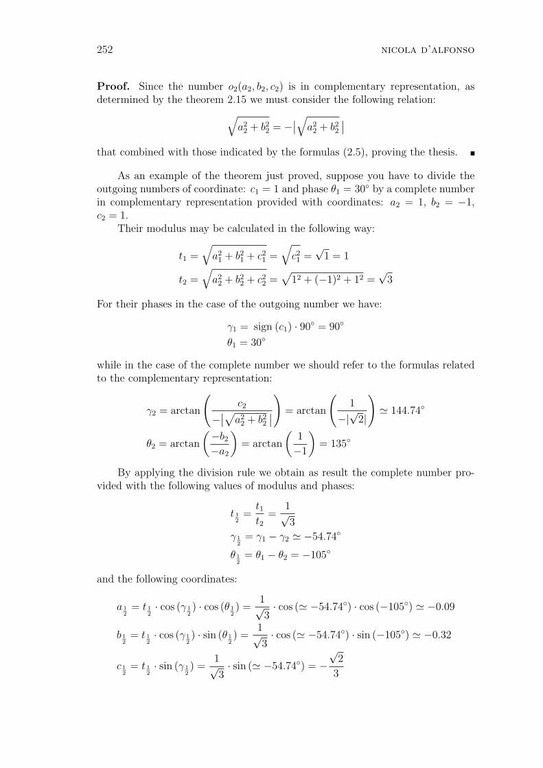
252 nicola d’alfonso
Proof. Since the number o2(a2, b2, c2) is in complementary representation, asdetermined by the theorem 2.15 we must consider the following relation:
√a2
2 + b22 = −
∣∣√
a22 + b2
2
∣∣
that combined with those indicated by the formulas (2.5), proving the thesis.
As an example of the theorem just proved, suppose you have to divide theoutgoing numbers of coordinate: c1 = 1 and phase θ1 = 30 by a complete numberin complementary representation provided with coordinates: a2 = 1, b2 = −1,c2 = 1.
Their modulus may be calculated in the following way:
t1 =√
a21 + b2
1 + c21 =
√c21 =
√1 = 1
t2 =√
a22 + b2
2 + c22 =
√12 + (−1)2 + 12 =
√3
For their phases in the case of the outgoing number we have:
γ1 = sign (c1) · 90 = 90
θ1 = 30
while in the case of the complete number we should refer to the formulas relatedto the complementary representation:
γ2 = arctan
(c2
−∣∣√a2
2 + b22
∣∣
)= arctan
(1
−|√2|
)' 144.74
θ2 = arctan
(−b2
−a2
)= arctan
(1
−1
)= 135
By applying the division rule we obtain as result the complete number pro-vided with the following values of modulus and phases:
t 12
=t1t2
=1√3
γ 12
= γ1 − γ2 ' −54.74
θ 12
= θ1 − θ2 = −105
and the following coordinates:
a 12
= t 12· cos (γ 1
2) · cos (θ 1
2) =
1√3· cos (' −54.74) · cos (−105) ' −0.09
b 12
= t 12· cos (γ 1
2) · sin (θ 1
2) =
1√3· cos (' −54.74) · sin (−105) ' −0.32
c 12
= t 12· sin (γ 1
2) =
1√3· sin (' −54.74) = −
√2
3
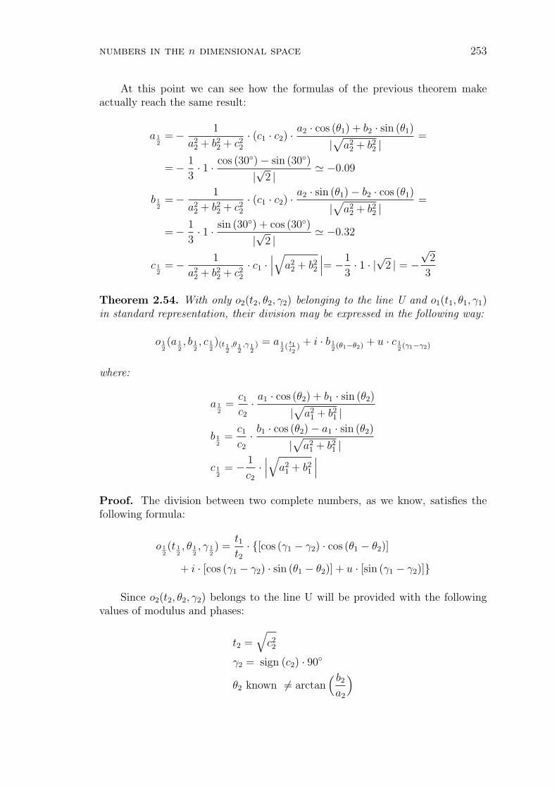
numbers in the n dimensional space 253
At this point we can see how the formulas of the previous theorem makeactually reach the same result:
a 12
=− 1
a22 + b2
2 + c22
· (c1 · c2) · a2 · cos (θ1) + b2 · sin (θ1)
|√
a22 + b2
2 |=
=− 1
3· 1 · cos (30)− sin (30)
|√2 | ' −0.09
b 12
=− 1
a22 + b2
2 + c22
· (c1 · c2) · a2 · sin (θ1)− b2 · cos (θ1)
|√
a22 + b2
2 |=
=− 1
3· 1 · sin (30) + cos (30)
|√2 | ' −0.32
c 12
=− 1
a22 + b2
2 + c22
· c1 ·∣∣∣√
a22 + b2
2
∣∣∣= −1
3· 1 · |
√2 | = −
√2
3
Theorem 2.54. With only o2(t2, θ2, γ2) belonging to the line U and o1(t1, θ1, γ1)in standard representation, their division may be expressed in the following way:
o 12(a 1
2, b 1
2, c 1
2)(t 1
2,θ 1
2,γ 1
2) = a 1
2(
t1t2
) + i · b 12(θ1−θ2) + u · c 1
2(γ1−γ2)
where:
a 12
=c1
c2
· a1 · cos (θ2) + b1 · sin (θ2)
|√
a21 + b2
1 |b 1
2=
c1
c2
· b1 · cos (θ2)− a1 · sin (θ2)
|√
a21 + b2
1 |c 1
2= − 1
c2
·∣∣∣√
a21 + b2
1
∣∣∣
Proof. The division between two complete numbers, as we know, satisfies thefollowing formula:
o 12(t 1
2, θ 1
2, γ 1
2) =
t1t2· [cos (γ1 − γ2) · cos (θ1 − θ2)]
+ i · [cos (γ1 − γ2) · sin (θ1 − θ2)] + u · [sin (γ1 − γ2)]
Since o2(t2, θ2, γ2) belongs to the line U will be provided with the followingvalues of modulus and phases:
t2 =√
c22
γ2 = sign (c2) · 90
θ2 known 6= arctan( b2
a2
)
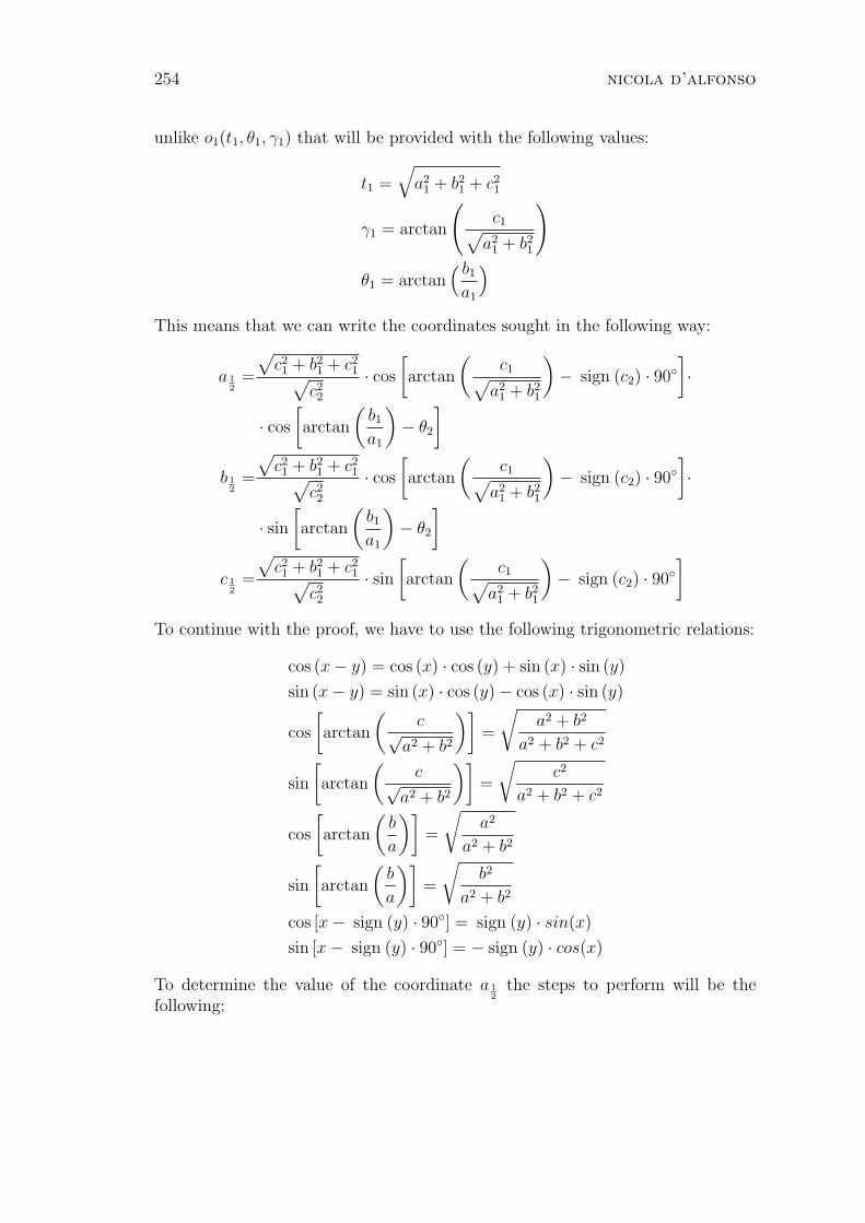
254 nicola d’alfonso
unlike o1(t1, θ1, γ1) that will be provided with the following values:
t1 =√
a21 + b2
1 + c21
γ1 = arctan
(c1√
a21 + b2
1
)
θ1 = arctan( b1
a1
)
This means that we can write the coordinates sought in the following way:
a 12
=
√c21 + b2
1 + c21√
c22
· cos
[arctan
(c1√
a21 + b2
1
)− sign (c2) · 90
]·
· cos
[arctan
(b1
a1
)− θ2
]
b 12
=
√c21 + b2
1 + c21√
c22
· cos
[arctan
(c1√
a21 + b2
1
)− sign (c2) · 90
]·
· sin[arctan
(b1
a1
)− θ2
]
c 12
=
√c21 + b2
1 + c21√
c22
· sin[arctan
(c1√
a21 + b2
1
)− sign (c2) · 90
]
To continue with the proof, we have to use the following trigonometric relations:
cos (x− y) = cos (x) · cos (y) + sin (x) · sin (y)
sin (x− y) = sin (x) · cos (y)− cos (x) · sin (y)
cos
[arctan
(c√
a2 + b2
)]=
√a2 + b2
a2 + b2 + c2
sin
[arctan
(c√
a2 + b2
)]=
√c2
a2 + b2 + c2
cos
[arctan
(b
a
)]=
√a2
a2 + b2
sin
[arctan
(b
a
)]=
√b2
a2 + b2
cos [x− sign (y) · 90] = sign (y) · sin(x)
sin [x− sign (y) · 90] = − sign (y) · cos(x)
To determine the value of the coordinate a 12
the steps to perform will be thefollowing:

numbers in the n dimensional space 255
a 12
= sign (c2) ·√
c21 + b2
1 + c21√
c22
·√
c21
a21 + b2
1 + c21
·
·[√
a21
a21 + b2
1
· cos (θ2) +
√b21
a21 + b2
1
· sin (θ2)
]
= sign (c2) ·√
c21√
c22
·√
a21 · cos (θ2) +
√b21 · sin (θ2)√
a21 + b2
1
To determine the value of the coordinate b 12
the steps to perform will be thefollowing:
b 12
= sign (c2) ·√
c21 + b2
1 + c21√
c22
·√
c21
a21 + b2
1 + c21
·
·[√
b21
a21 + b2
1
· cos (θ2)−√
a21
a21 + b2
1
· sin (θ2)
]
= sign (c2) ·√
c21√
c22
·√
b21 · cos (θ2)−
√a2
1 · sin (θ2)√a2
1 + b21
To determine the value of the coordinate c 12
the steps to perform will be thefollowing:
c 12
= − sign (c2) ·√
c21 + b2
1 + c21√
c22
·√
a21 + b2
1
a21 + b2
1 + c21
= − sign (c2) · 1√c22
·√
a21 + b2
1
These relations are valid in general, in the precise sense that they are also ableto include cases where the coefficients a1,b1,c1 are zero (provided that o1(a1, b1, c1)remains in the context of the complete numbers not belonging in the line U).
The only limitation in this regard is the need to avoid the following situation:
c22 = 0
which confirms the impossibility to divide a complete number o(t, θ, γ) for zero(characterized by the values c2 that make the above mentioned condition true).
Wanting to find relations that satisfy the division rule as a function of theeffective coordinates of the complete numbers involved, we must adopt for thecoefficients a,b,c the convention
√x2 = x, with the exception of c2 for which we
should adopt the convention√
x2 = |x|. The reason is simple because if we adoptfor c2 the usual convention, we will have:
sign (c2)√c22
=1
|c2|
256 nicola d’alfonso
and therefore a result of the division that depends on the modulus of the coordi-nate c2. While adopting
√x2 = |x| we will have:
sign (c2)√c22
=1
c2
and therefore a result of the division that depends on the effective value of thiscoordinate.
The relations obtained will be the following:
a 12
=c1
c2
· a1 · cos (θ2) + b1 · sin (θ2)√a2
1 + b21
b 12
=c1
c2
· b1 · cos (θ2)− a1 · sin (θ2)√a2
1 + b21
c 12
= − 1
c2
·√
a21 + b2
1
(2.6)
Since the number o1(a1, b1, c1) is in standard representation, as determinedby the theorem 2.11 we must consider the following relation:
√a2
1 + b21 =
∣∣√
a21 + b2
1
∣∣
that combined with those indicated by the formulas (2.6), proving the thesis.
As an example of the theorem just proved, suppose you have to divide thecomplete number in standard representation provided with coordinates: a1 = 1,b1 = −1, c1 = 1 by an outgoing numbers of coordinate:c2 = 1 and phase θ2 = 30.
Their modulus may be calculated in the following way:
t1 =√
a21 + b2
1 + c21 =
√12 + (−1)2 + 12 =
√3
t2 =√
a22 + b2
2 + c22 =
√c22 =
√1 = 1
For their phases in the case of the outgoing number we have:
γ2 = sign (c2) · 90 = 90
θ2 = 30
while in the case of the complete number we should refer to the formulas relatedto the standard representation:
γ1 = arctan
(c1∣∣√a21 + b2
1
∣∣
)= arctan
(1
|√2|
)' 35.26
θ1 = arctan
(b1
a1
)= arctan
(−1
1
)= −45
numbers in the n dimensional space 257
By applying the division rule we obtain as result the complete number pro-vided with the following values of modulus and phases:
t 12
=t1t2
=√
3
γ 12
= γ1 − γ2 ' −54.74
θ 12
= θ1 − θ2 = −75
and the following coordinates:
a 12
= t 12· cos (γ 1
2) · cos (θ 1
2) =
√3 · cos (' −54.74) · cos (−75) ' 0.26
b 12
= t 12· cos (γ 1
2) · sin (θ 1
2) =
√3 · cos (' −54.74) · sin (−75) ' −0.97
c 12
= t 12· sin (γ 1
2) =
√3 · sin (' −54.74) = −
√2
At this point we can see how the formulas of the previous theorem makeactually reach the same result:
a 12
=c1
c2
· a1 · cos (θ2) + b1 · sin (θ2)
|√
a21 + b2
1 |=
cos (30)− sin (30)
|√2 | ' 0.26
b 12
=c1
c2
· b1 · cos (θ2)− a1 · sin (θ2)
|√
a21 + b2
1 |=− cos (30)− sin (30)
|√2 | ' −0.97
c 12
= − 1
c2
·∣∣∣√
a21 + b2
1
∣∣∣= −√
2
Theorem 2.55. With only o2(t2, θ2, γ2) belonging to the line U and o1(t1, θ1, γ1)in complementary representation, their division may be expressed in the followingway:
o 12(a 1
2, b 1
2, c 1
2)(t 1
2,θ 1
2,γ 1
2) = a 1
2(
t1t2
) + i · b 12(θ1−θ2) + u · c 1
2(γ1−γ2)
where:
a 12
= −c1
c2
· a1 · cos (θ2) + b1 · sin (θ2)
|√
a21 + b2
1 |b 1
2= −c1
c2
· b1 · cos (θ2)− a1 · sin (θ2)
|√
a21 + b2
1 |c 1
2=
1
c2
·∣∣∣√
a21 + b2
1
∣∣∣
Proof. Since the number o1(a1, b1, c1) is in complementary representation, asdetermined by the theorem 2.15 we must consider the following relation:
√a2
1 + b21 = −
∣∣√
a21 + b2
1
∣∣
that combined with those indicated by the formulas (2.6), proving the thesis.

258 nicola d’alfonso
As an example of the theorem just proved, suppose you have to divide acomplete number in complementary representation provided with coordinates:a2 = 1, b2 = −1, c2 = 1 by the outgoing numbers of coordinate: c1 = 1 and phaseθ1 = 30.
Their modulus may be calculated in the following way:
t1 =√
a21 + b2
1 + c21 =
√12 + (−1)2 + 12 =
√3
t2 =√
a22 + b2
2 + c22 =
√c22 =
√1 = 1
For their phases in the case of the outgoing number we have:
γ2 = sign (c2) · 90 = 90
θ2 = 30
while in the case of the complete number we should refer to the formulas relatedto the complementary representation:
γ1 = arctan
(c1
−∣∣√a2
1 + b21
∣∣
)= arctan
(1
−|√2|
)' 144.74
θ1 = arctan
(−b1
−a1
)= arctan
(1
−1
)= 135
By applying the division rule we obtain as result the complete number pro-vided with the following values of modulus and phases:
t 12
=t1t2
=√
3
γ 12
= γ1 − γ2 ' 54.74
θ 12
= θ1 − θ2 = 105
and the following coordinates:
a 12
= t 12· cos (γ 1
2) · cos (θ 1
2) =
√3 · cos (' 54.74) · cos (105) ' −0.26
b 12
= t 12· cos (γ 1
2) · sin (θ 1
2) =
√3 · cos (' 54.74) · sin (105) ' 0.97
c 12
= t 12· sin (γ 1
2) =
√3 · sin (' 54.74) =
√2
At this point we can see how the formulas of the previous theorem makeactually reach the same result:
a 12
= −c1
c2
· a1 · cos (θ2) + b1 · sin (θ2)
|√
a21 + b2
1 |= −cos (30)− sin (30)
|√2 | ' −0.26
b 12
= −c1
c2
· b1 · cos (θ2)− a1 · sin (θ2)
|√
a21 + b2
1 |= −− cos (30)− sin (30)
|√2 | ' 0.97
c 12
=1
c2
·∣∣∣√
a21 + b2
1
∣∣∣=√
2

numbers in the n dimensional space 259
Theorem 2.56. With o1(t1, θ1, γ1) and o2(t2, θ2, γ2) both belonging to the line U,their division may be expressed in the following way:
o 12(a 1
2, b 1
2, c 1
2)(t 1
2,θ 1
2,γ 1
2) = a 1
2(
t1t2
) + i · b 12(θ1−θ2) + u · c 1
2(γ1−γ2)
where:
a 12
=c1
c2
· cos (θ1 − θ2)
b 12
=c1
c2
· sin (θ1 − θ2)
c 12
= 0
Proof. The division between two complete numbers, as we know, satisfies thefollowing formula:
o 12(t 1
2, θ 1
2, γ 1
2) =
t1t2· [cos (γ1 − γ2) · cos (θ1 − θ2)]+
+ i · [cos (γ1 − γ2) · sin (θ1 − θ2)] + u · [sin (γ1 − γ2)]Since o1(t1, θ1, γ1) and o2(t2, θ2, γ2) belong to the line U will be provided with
the following values of modulus and phases:
t1 =√
c21
t2 =√
c22
γ1 = sign (c1) · 90
γ2 = sign (c2) · 90
θ1 known 6= arctan( b1
a1
)
θ2 known 6= arctan( b2
a2
)
This means that we can write the coordinates sought in the following way:
a 12
=
√c21√
c22
· cos [ sign (c1) · 90 − sign (c2) · 90] · cos (θ1 − θ2)
b 12
=
√c21√
c22
· cos [ sign (c1) · 90 − sign (c2) · 90] · sin (θ1 − θ2)
c 12
=
√c21√
c22
· sin [ sign (c1) · 90 − sign (c2) · 90]
Considering that when c1 and c2 have the same sign we obtained:
cos [ sign (c1) · 90 − sign (c2) · 90] = cos (±0) = 1 = sign (c1) · sign (c2)
sin [ sign (c1) · 90 − sign (c2) · 90] = sin (±0) = 0
260 nicola d’alfonso
and that when they have the opposite sign we obtained:
cos [ sign (c1) · 90 − sign (c2) · 90] = cos (±180) = −1 = sign (c1) · sign (c2)
sin [ sign (c1) · 90 − sign (c2) · 90] = sin (±180) = 0
we can write:
a 12
= sign (c1) · sign (c2) ·√
c21√
c22
· cos (θ1 − θ2)
b 12
= sign (c1) · sign (c2) ·√
c21√
c22
· sin (θ1 − θ2)
c 12
= 0
Wanting to find relations that satisfy the division rule as a function of theeffective coordinates of the complete numbers involved, we must adopt for thecoefficients c1,c2 the convention
√x2 = |x|. In fact in this way we obtain:
sign (c1) ·√
c21 = c1
sign (c2)√c22
=1
c2
and therefore a result of the division that depends on the effective values of thesecoordinates. The relation that we obtain following these conventions proves thethesis.
As an example of the theorem just proved, suppose you have to divide theoutgoing numbers of coordinate: c1 = 1 and phase θ1 = 30 by the outgoingnumber of coordinate: c2 = 1 and phase θ2 = 30.
Their modulus may be calculated in the following way:
t1 =√
a21 + b2
1 + c21 =
√c21 =
√1 = 1
t2 =√
a22 + b2
2 + c22 =
√c22 =
√1 = 1
For their phases we have:
γ1 = sign (c1) · 90 = 90
γ2 = sign (c2) · 90 = 90
θ1 = 30
θ2 = 30
By applying the division rule we obtain as result the complete number pro-vided with the following values of modulus and phases:
t 12
=t1t2
= 1
γ 12
= γ1 − γ2 = 0
θ 12
= θ1 − θ2 = 0
numbers in the n dimensional space 261
and the following coordinates:
a 12
= t 12· cos (γ 1
2) · cos (θ 1
2) = 1 · cos (0) · cos (0) = 1
b 12
= t 12· cos (γ 1
2) · sin (θ 1
2) = 1 · cos (0) · sin (0) = 0
c 12
= t 12· sin (γ 1
2) = 1 · sin (0) = 0
At this point we can see how the formulas of the previous theorem makeactually reach the same result:
a 12
=
√c21√
c22
· cos (θ1 − θ2) = 1 · cos (0) = 1
b 12
=
√c21√
c22
· sin (θ1 − θ2) = 1 · sin (0) = 0
c 12
= 0
Theorem 2.57. For the operation of division is defined indivisible the completenumber 0, namely for:
o1(t1, θ1, γ1) = 0
we have:o1(t1, θ1, γ1)
o2(t2, θ2, γ2)= 0
Proof. t1,θ1,γ1,t2,θ2,γ2 being real numbers, we can write:
t 12
=t1t2
=0
t2= 0
θ 12
= θ1 − θ2 = θ1 − indeterminate = indeterminate
γ 12
= γ1 − γ2 = γ1 − indeterminate = indeterminate
proving the thesis.
Theorem 2.58. For the operation of division is defined neuter the complete num-ber 1(S), namely for:
o2(a2, b2, c2)(S) = 1(S)
we have:o1(t1, θ1, γ1)
o2(t2, θ2, γ2)= o1(t1, θ1, γ1)
Proof. t1,θ1,γ1,t2,θ2,γ2 being real numbers, we can write:
t 12
=t1t2
=t11
= t1
θ 12
= θ1 − θ2 = θ1 − 0 = θ1
γ 12
= γ1 − γ2 = γ1 − 0 = γ1
proving the thesis.

262 nicola d’alfonso
Theorem 2.59. For the operation of division is defined identical the same positionwith respect to the origin, namely for:
o2(a2, b2, c2) = o2(a1, b1, c1)
we have:o1(t1, θ1, γ1)
o2(t2, θ2, γ2)= 1(S)
Proof. t1,θ1,γ1,t2,θ2,γ2 being real numbers, we can write:
t 12
=t1t2
=t1t1
= 1
θ 12
= θ1 − θ2 = θ1 − θ1 = 0
γ 12
= γ1 − γ2 = γ1 − γ1 = 0
proving the thesis.
Theorem 2.60. It is valid the invariantive property, namely:
o1(t1, θ1, γ1)
o2(t2, θ2, γ2)=
[o1(t1, θ1, γ1) · o3(t3, θ3, γ3)]
[o2(t2, θ2, γ2) · o3(t3, θ3, γ3)]
o1(t1, θ1, γ1)
o2(t2, θ2, γ2)=
o1(t1,θ1,γ1)o3(t3,θ3,γ3)
o2(t2,θ2,γ2)o3(t3,θ3,γ3)
Proof. t1,θ1,γ1,t2,θ2,γ2,t3,θ3,γ3 being real numbers, we can write:
t 12
=t1t2
θ 12
= (θ1 − θ2)
γ 12
= (γ1 − γ2)
t (1·3)(2·3)
=t1 · t3t2 · t3 =
t1t2
θ (1·3)(2·3)
= (θ1 + θ3)− (θ2 + θ3) = θ1 − θ2
γ (1·3)(2·3)
= (γ1 + γ3)− (γ2 + γ3) = γ1 − γ2
t ( 13 )
( 23 )
=t1t3t2t3
=t1t2
θ ( 13 )
( 23 )
= (θ1 − θ3)− (θ2 − θ3) = θ1 − θ2
γ ( 13 )
( 23 )
= (γ1 − γ3)− (γ2 − γ3) = γ1 − γ2
proving the thesis.
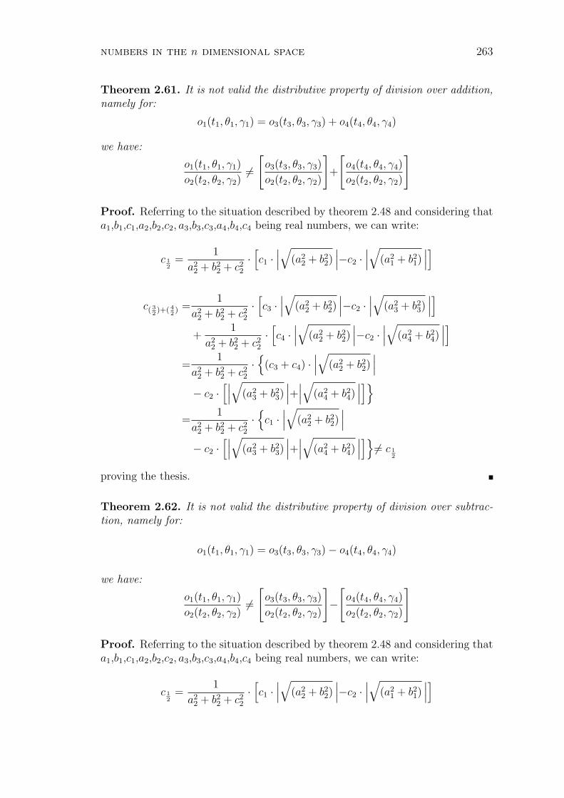
numbers in the n dimensional space 263
Theorem 2.61. It is not valid the distributive property of division over addition,namely for:
o1(t1, θ1, γ1) = o3(t3, θ3, γ3) + o4(t4, θ4, γ4)
we have:
o1(t1, θ1, γ1)
o2(t2, θ2, γ2)6=
[o3(t3, θ3, γ3)
o2(t2, θ2, γ2)
]+
[o4(t4, θ4, γ4)
o2(t2, θ2, γ2)
]
Proof. Referring to the situation described by theorem 2.48 and considering thata1,b1,c1,a2,b2,c2, a3,b3,c3,a4,b4,c4 being real numbers, we can write:
c 12
=1
a22 + b2
2 + c22
·[c1 ·
∣∣∣√
(a22 + b2
2)∣∣∣−c2 ·
∣∣∣√
(a21 + b2
1)∣∣∣]
c( 32)+( 4
2) =
1
a22 + b2
2 + c22
·[c3 ·
∣∣∣√
(a22 + b2
2)∣∣∣−c2 ·
∣∣∣√
(a23 + b2
3)∣∣∣]
+1
a22 + b2
2 + c22
·[c4 ·
∣∣∣√
(a22 + b2
2)∣∣∣−c2 ·
∣∣∣√
(a24 + b2
4)∣∣∣]
=1
a22 + b2
2 + c22
·
(c3 + c4) ·∣∣∣√
(a22 + b2
2)∣∣∣
− c2 ·[∣∣∣
√(a2
3 + b23)
∣∣∣+∣∣∣√
(a24 + b2
4)∣∣∣]
=1
a22 + b2
2 + c22
·
c1 ·∣∣∣√
(a22 + b2
2)∣∣∣
− c2 ·[∣∣∣
√(a2
3 + b23)
∣∣∣+∣∣∣√
(a24 + b2
4)∣∣∣]6= c 1
2
proving the thesis.
Theorem 2.62. It is not valid the distributive property of division over subtrac-tion, namely for:
o1(t1, θ1, γ1) = o3(t3, θ3, γ3)− o4(t4, θ4, γ4)
we have:
o1(t1, θ1, γ1)
o2(t2, θ2, γ2)6=
[o3(t3, θ3, γ3)
o2(t2, θ2, γ2)
]−
[o4(t4, θ4, γ4)
o2(t2, θ2, γ2)
]
Proof. Referring to the situation described by theorem 2.48 and considering thata1,b1,c1,a2,b2,c2, a3,b3,c3,a4,b4,c4 being real numbers, we can write:
c 12
=1
a22 + b2
2 + c22
·[c1 ·
∣∣∣√
(a22 + b2
2)∣∣∣−c2 ·
∣∣∣√
(a21 + b2
1)∣∣∣]
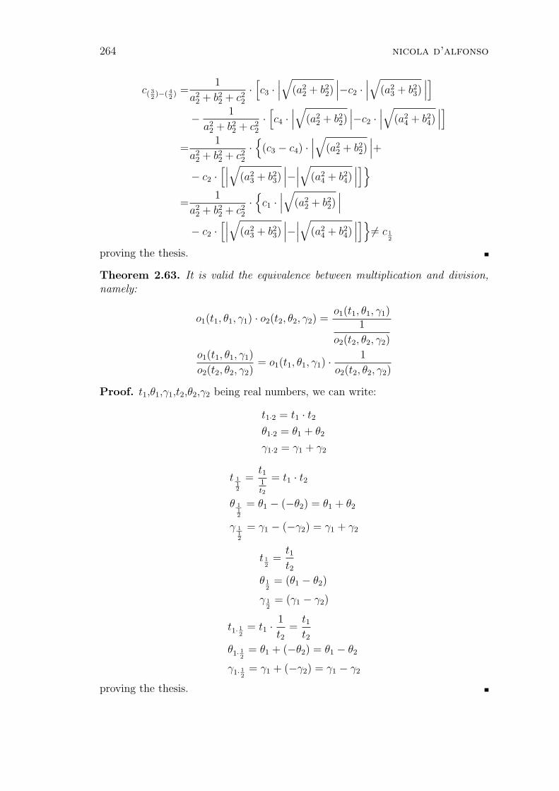
264 nicola d’alfonso
c( 32)−( 4
2) =
1
a22 + b2
2 + c22
·[c3 ·
∣∣∣√
(a22 + b2
2)∣∣∣−c2 ·
∣∣∣√
(a23 + b2
3)∣∣∣]
− 1
a22 + b2
2 + c22
·[c4 ·
∣∣∣√
(a22 + b2
2)∣∣∣−c2 ·
∣∣∣√
(a24 + b2
4)∣∣∣]
=1
a22 + b2
2 + c22
·
(c3 − c4) ·∣∣∣√
(a22 + b2
2)∣∣∣+
− c2 ·[∣∣∣
√(a2
3 + b23)
∣∣∣−∣∣∣√
(a24 + b2
4)∣∣∣]
=1
a22 + b2
2 + c22
·
c1 ·∣∣∣√
(a22 + b2
2)∣∣∣
− c2 ·[∣∣∣
√(a2
3 + b23)
∣∣∣−∣∣∣√
(a24 + b2
4)∣∣∣]6= c 1
2
proving the thesis.
Theorem 2.63. It is valid the equivalence between multiplication and division,namely:
o1(t1, θ1, γ1) · o2(t2, θ2, γ2) =o1(t1, θ1, γ1)
1
o2(t2, θ2, γ2)
o1(t1, θ1, γ1)
o2(t2, θ2, γ2)= o1(t1, θ1, γ1) · 1
o2(t2, θ2, γ2)
Proof. t1,θ1,γ1,t2,θ2,γ2 being real numbers, we can write:
t1·2 = t1 · t2θ1·2 = θ1 + θ2
γ1·2 = γ1 + γ2
t 112
=t11t2
= t1 · t2
θ 112
= θ1 − (−θ2) = θ1 + θ2
γ 112
= γ1 − (−γ2) = γ1 + γ2
t 12
=t1t2
θ 12
= (θ1 − θ2)
γ 12
= (γ1 − γ2)
t1· 12
= t1 · 1
t2=
t1t2
θ1· 12
= θ1 + (−θ2) = θ1 − θ2
γ1· 12
= γ1 + (−γ2) = γ1 − γ2
proving the thesis.

numbers in the n dimensional space 265
2.6. N-th power
Definition 2.64. In the space RIU we can define n-th power of the completenumber o(t, θ, γ), with n (natural number) known as exponent and o(t, θ, γ) knownas base, as the number o↑n(t↑n, θ↑n, γ↑n) also represented with the symbol o(t, θ, γ)n
that satisfies the following conditions:
1. o(t, θ, γ)n = o(t, θ, γ) · ... · o(t, θ, γ) for n > 0
2. o(t, θ, γ)n = o(t,θ,γ)o(t,θ,γ)
= 1 for n = 0
3. o(t, θ, γ)n =1
o(t, θ, γ)
. . .
o(t, θ, γ)
for n < 0
4. n > 0 for o(t, θ, γ) = 0
We note that the term o(t, θ, γ) in the first and third conditions is intended toappear |n| times.
The first condition defines the repeated multiplication of the base by itself apositive number of times, the second a zero number of times, and finally the thirda negative number of times. All these conditions correspond to require:
t↑n = tn
θ↑n = θ · nγ↑n = γ · n
The fourth condition gets its own justification by the impossibility of definingthe n-th power module when to be multiplied by itself a zero number or a negativenumber of times is just the 0, because in this case would be present the followingdivisions for 0:
o(t, θ, γ)n =0
0= 1 for n = 0
o(t, θ, γ)n =1
0
. . .
0
for n < 0 with 0 that appears —n— times
Theorem 2.65. It is valid the product property of exponents, namely:
(on)m = on·m
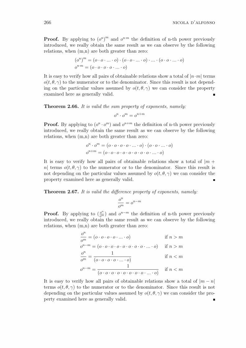
266 nicola d’alfonso
Proof. By applying to (on)m and on·m the definition of n-th power previouslyintroduced, we really obtain the same result as we can observe by the followingrelations, when (m,n) are both greater than zero:
(on)m = (o · o · ... · o) · (o · o · ... · o) · ... · (o · o · ... · o)on·m = (o · o · o · o · ... · o)
It is easy to verify how all pairs of obtainable relations show a total of |n ·m| termso(t, θ, γ) to the numerator or to the denominator. Since this result is not depend-ing on the particular values assumed by o(t, θ, γ) we can consider the propertyexamined here as generally valid.
Theorem 2.66. It is valid the sum property of exponents, namely:
on · om = on+m
Proof. By applying to (on · om) and on+m the definition of n-th power previouslyintroduced, we really obtain the same result as we can observe by the followingrelations, when (m,n) are both greater than zero:
on · om = (o · o · o · o · ... · o) · (o · o · ... · o)on+m = (o · o · o · o · o · o · o · o · ... · o)
It is easy to verify how all pairs of obtainable relations show a total of |m +n| terms o(t, θ, γ) to the numerator or to the denominator. Since this result isnot depending on the particular values assumed by o(t, θ, γ) we can consider theproperty examined here as generally valid.
Theorem 2.67. It is valid the difference property of exponents, namely:
on
om= on−m
Proof. By applying to ( on
om ) and on−m the definition of n-th power previouslyintroduced, we really obtain the same result as we can observe by the followingrelations, when (m,n) are both greater than zero:
on
om= (o · o · o · o · ... · o) if n > m
on−m = (o · o · o · o · o · o · o · o · ... · o) if n > m
on
om=
1
(o · o · o · o · ... · o) if n < m
on−m =1
(o · o · o · o · o · o · o · o · ... · o) if n < m
It is easy to verify how all pairs of obtainable relations show a total of |m− n|terms o(t, θ, γ) to the numerator or to the denominator. Since this result is notdepending on the particular values assumed by o(t, θ, γ) we can consider the pro-perty examined here as generally valid.
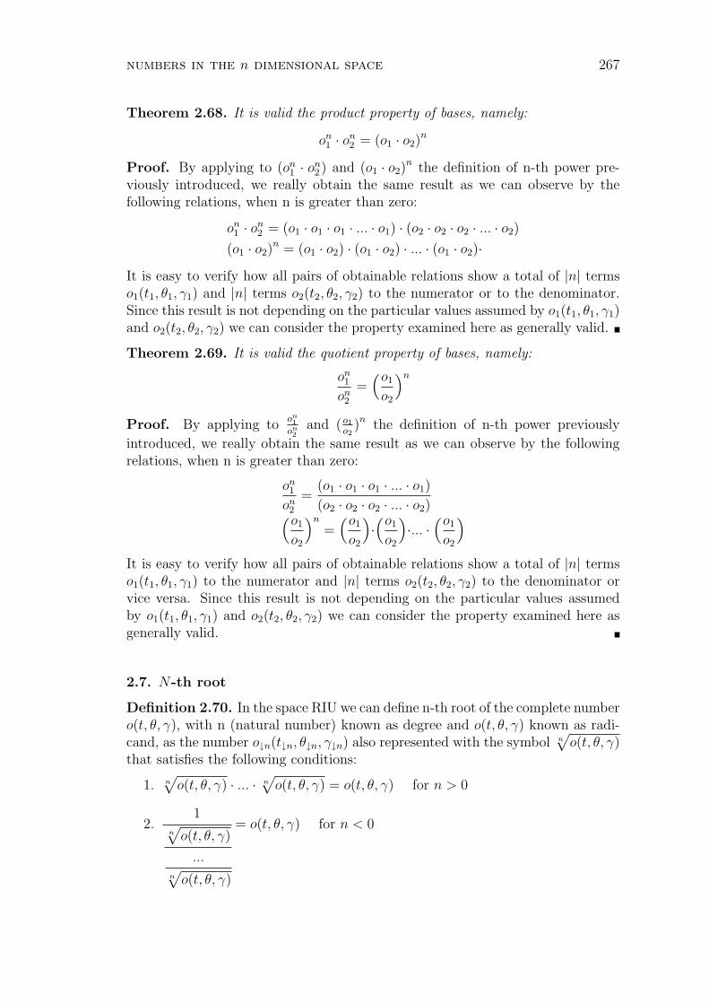
numbers in the n dimensional space 267
Theorem 2.68. It is valid the product property of bases, namely:
on1 · on
2 = (o1 · o2)n
Proof. By applying to (on1 · on
2 ) and (o1 · o2)n the definition of n-th power pre-
viously introduced, we really obtain the same result as we can observe by thefollowing relations, when n is greater than zero:
on1 · on
2 = (o1 · o1 · o1 · ... · o1) · (o2 · o2 · o2 · ... · o2)
(o1 · o2)n = (o1 · o2) · (o1 · o2) · ... · (o1 · o2)·
It is easy to verify how all pairs of obtainable relations show a total of |n| termso1(t1, θ1, γ1) and |n| terms o2(t2, θ2, γ2) to the numerator or to the denominator.Since this result is not depending on the particular values assumed by o1(t1, θ1, γ1)and o2(t2, θ2, γ2) we can consider the property examined here as generally valid.
Theorem 2.69. It is valid the quotient property of bases, namely:
on1
on2
=(o1
o2
)n
Proof. By applying toon1
on2
and (o1
o2)n the definition of n-th power previously
introduced, we really obtain the same result as we can observe by the followingrelations, when n is greater than zero:
on1
on2
=(o1 · o1 · o1 · ... · o1)
(o2 · o2 · o2 · ... · o2)(o1
o2
)n
=(o1
o2
)·(o1
o2
)·... ·
(o1
o2
)
It is easy to verify how all pairs of obtainable relations show a total of |n| termso1(t1, θ1, γ1) to the numerator and |n| terms o2(t2, θ2, γ2) to the denominator orvice versa. Since this result is not depending on the particular values assumedby o1(t1, θ1, γ1) and o2(t2, θ2, γ2) we can consider the property examined here asgenerally valid.
2.7. N-th root
Definition 2.70. In the space RIU we can define n-th root of the complete numbero(t, θ, γ), with n (natural number) known as degree and o(t, θ, γ) known as radi-cand, as the number o↓n(t↓n, θ↓n, γ↓n) also represented with the symbol n
√o(t, θ, γ)
that satisfies the following conditions:
1. n√
o(t, θ, γ) · ... · n√
o(t, θ, γ) = o(t, θ, γ) for n > 0
2.1
n√
o(t, θ, γ)
...n√
o(t, θ, γ)
= o(t, θ, γ) for n < 0
268 nicola d’alfonso
3. θ↓n = θn, γ↓n = γ
n
4. n 6= 0 for any o(t, θ, γ)
5. n ≥ 0 for o(t, θ, γ) = 0
6. n√
t > 0, t > 0
We note that the term n√
o(t, θ, γ) in the first and second conditions is intendedto appear |n| times.
The first condition defines the repeated multiplication of the root by itselfa positive number of times, while the second a negative number of times. Boththese conditions correspond to require:
t↓n =n√
t
θ↓n =θ + k · 360
nfor k = ±1,±2,±3,±4, ...
γ↓n =γ + k · 360
nfor k = ±1,±2,±3,±4, ...
The third condition gets its own justification by the necessity of defining then-th root in an univocal way. In fact, when that condition is not valid, there aren2 different complete numbers able to satisfy such definition: one for each distinctpair of phases θ↓n, γ↓n given by the relations seen above.
Also the fourth condition gets its own justification by the necessity of definingthe n-th root in an univocal way. In fact when that condition is not valid, themultiplication of the root by itself a number of times equal to 0 would require theuse of the following expression:
n√
o(t, θ, γ)n√
o(t, θ, γ)= 1
that would be satisfied by several values of n√
o(t, θ, γ).The fifth condition gets its own justification by the impossibility of defining
values of n-th root that multiplied by itself a negative number of times are ableto give as the result just 0 value. In fact the following expression:
1n√
o(t, θ, γ)
...n√
o(t, θ, γ)
= 0 for n < 0, n√
o(t, θ, γ) appears —n— times
requires the existence of a divisor of 1 that can assign to it a quotient equal to 0:a thing that we know impossible.
The sixth condition gets its own justification by the need to make acceptablethe n-th root in regard the modulus t of the complete number o(t, θ, γ).
numbers in the n dimensional space 269
Theorem 2.71. It is valid the product property of degrees, namely:
m
√n√
o = m·n√o
Proof. By applying the principle according to which two numbers are equal ifand only if they remain as such, also once we raise them to the same power, we canraise the two member of the previous equality to the number (m · n), obtaining:
(m
√n√
o
)(m·n)
= ( m·n√o )(m·n)
At this point, we can verify the validity of the starting equality showing how thetwo members thus obtained are actually equal.
Considering the value m√
n√
o of the first member as a complete number, it ispossible to apply to it the theorem 2.65 concerning the product of exponents ofthe n-th power, obtaining:
(m
√n√
o
)(m·n)
=
[(m
√n√
o
)m]n
Then applying to this member the definition of n-th root, we obtain:[(
m
√n√
o
)m]n
= ( n√
o )n
= o
By applying the same definition to the second member we obtain an equivalentfinal result:
( m·n√o )(m·n)
= o
Theorem 2.72. It is valid the product property of radicands, namely:
n√
o1 · n√
o2 = n√
o1 · o2
Proof. By applying the principle according to which two numbers are equal ifand only if they remain as such, also once we raise them to the same power, wecan raise the two member of the previous equality to the number n, obtaining:
( n√
o1 · n√
o2 )n
= ( n√
o1 · o2 )n
At this point, we can verify the validity of the starting equality showing how thetwo members thus obtained are actually equal.
Considering the values n√
o1 and n√
o2 of the first member as the completenumbers, it is possible to apply to them the theorem 2.68 concerning the productof bases of the n-th power, obtaining:
( n√
o1 · n√
o2 )n
= ( n√
o1 )n · ( n
√o2 )
n
Then applying to two factors of this member the definition of n-th root, we obtain:
( n√
o1 )n · ( n
√o2 )
n= o1 · o2
By applying the same definition to the second member we obtain an equivalentfinal result:
( n√
o1 · o2 )n
= o1 · o2
270 nicola d’alfonso
Theorem 2.73. It is valid the quotient property of radicands, namely:
n√
o1
n√
o2
= n
√o1
o2
Proof. By applying the principle according to which two numbers are equal ifand only if they remain as such, also once we raise them to the same power, wecan raise the two member of the previous equality to the number n, obtaining:
(n√
o1
n√
o2
)n
=
(n
√o1
o2
)n
At this point, we can verify the validity of the starting equality showing how thetwo members thus obtained are actually equal.
Considering the values n√
o1 and n√
o2 of the first member as the completenumbers, it is possible to apply to them the theorem 2.69 concerning the quotientof bases of the n-th power, obtaining:
(n√
o1
n√
o2
)n
=( n√
o1 )n
( n√
o2 )n
Then applying to two factors of this member the definition of n-th root, we obtain:
( n√
o1 )n
( n√
o2 )n =o1
o2
By applying the same definition to the second member we obtain an equivalentfinal result: (
n
√o1
o2
)n
=o1
o2
2.8. Power with rational exponent
Definition 2.74. In the space RIU we can define power with rational expo-
nentm
n(n,m both natural numbers) of the complete number o(t, θ, γ), with
m
nknown as rational exponent and o(t, θ, γ) known as base, as the number
o↑m↓n(t↑m↓n, θ↑m↓n, γ↑m↓n) also represented with the symbol o(t, θ, γ)mn or
n√
o(t, θ, γ)m that satisfies the following conditions:
1.[
n√
o(t, θ, γ)m]n
= o(t, θ, γ)m
2. m > 0 for o(t, θ, γ) = 0
3. n 6= 0 for any o(t, θ, γ)m and therefore for any o(t, θ, γ)
numbers in the n dimensional space 271
4. n ≥ 0 for o(t, θ, γ)m = 0 and therefore for o(t, θ, γ) = 0
5. θ↑m↓n = θ·mn
, γ↑m↓n = γ·mn
6. n√
tm > 0, tm > 0
7. n√
t > 0, t > 0
The first condition defines the power with rational exponent as a n-th rootof a m-th power.
The second condition is required for the correct definition of the m-th power.The third, the fourth, the fifth and the sixth conditions are required for the
correct definition of n-th root.The seventh condition is required to make possible the reversal of the order
between root and power, namely to write:[
n√
o(t, θ, γ)]m
and therefore:(
n√
t )m
Theorem 2.75. It is valid the inversion property between root and power, namely:
omn = ( n
√o )
m
Proof. For the proof we will make reference to the following formulation of theproperty just introduced:
n√
om = ( n√
o )m
By applying the principle according to which two numbers are equal if and onlyif they remain as such, also once we raise them to the same power, we can raisethe two member of the previous equality to the number n obtaining:
(n√
om)n
= [( n√
o )m
]n
At this point, we can verify the validity of the starting equality showing how thetwo members thus obtained are actually equal.
Considering the value n√
o of the second member as a complete number, it ispossible to apply to it the theorem 2.65 concerning the product of exponents ofthe n-th power, obtaining:
[( n√
o )m
]n
= ( n√
o )m·n
= ( n√
o )n·m
= [( n√
o )n]m
Then applying to this member the definition of n-th root , we obtain:
[( n√
o )n]m
= om
By applying the same definition to the first member we obtain an equivalent finalresult: (
n√
om)n
= om
272 nicola d’alfonso
Theorem 2.76. It is valid the equivalence property between exponent and degree,namely:
omn = o
m·pn·p
Proof. For the proof we will make reference to the following formulation of theproperty just introduced:
n√
om = n·p√om·p
By applying the principle according to which two numbers are equal if and onlyif they remain as such, also once we raise them to the same power, we can raisethe two member of the previous equality to the number (n · p) obtaining:
(n√
om)(n·p)
= ( n·p√om·p )(n·p)
At this point, we can verify the validity of the starting equality showing how thetwo members thus obtained are actually equal.
By applying to the first member the theorem 2.75 concerning the inversionbetween root and power of the power with rational exponent, we obtain:
(n√
om)(n·p)
= [( n√
o )m
](n·p)
Considering the value n√
o of this member as a complete number, it is possibleto apply to it the theorem 2.65 concerning the product of exponents of the n-thpower, obtaining:
[( n√
o )m
](n·p)
= ( n√
o )m·n·p
== ( n√
o )n·m·p
= [( n√
o )n](m·p)
Then applying to this member the definition of n-th root , we obtain:
[( n√
o )n](m·p)
= om·p
By applying the same definition to the second member we obtain an equivalentfinal result:
( n·p√om·p )(n·p)
= om·p
Theorem 2.77. It is valid the product property of rational exponents,namely:
(omn )
pq = o
mn· pq = o
m·pn·p
Proof. For the proof we will make reference to the following formulation of theproperty just introduced:
( n√
om )pq = n·q√om·p
At this point, we can verify the validity of the starting equality showing how thetwo members thus obtained are actually equal.
Let us start expressing the first member in the following way:
( n√
om )pq =
q
√( n√
om )p
numbers in the n dimensional space 273
Considering the value om of this member as a complete number, it is possible toapply to it the theorem 2.75 concerning the inversion between root and power ofthe power with rational exponent, obtaining:
q
√( n√
om )p
=q
√n
√(om)p
Then applying to this member the theorem 2.71 concerning the product of degreesof the n-th root and the theorem 2.65 concerning the product of exponents of then-th power, we obtain an expression coincident with the second member:
q
√n
√(om)p = q·n√om·p
Theorem 2.78. It is valid the sum property of rational exponents, namely:
(omn ) · (o p
q ) = o(mn
+ pq) = o
(m·q)+(p·n)n·q
Proof. For the proof we will make reference to the following formulation of theproperty just introduced:
n√
om · q√
op =n·q√
o(m·q+p·n)
At this point, we can verify the validity of the starting equality showing how thetwo members thus obtained are actually equal.
By applying to the first member the theorem 2.76 concerning the equivalencebetween exponent and degree of the power with rational exponent, we obtain:
n√
om · q√
op = n·q√om·q · q·n√op·n
Considering the values om·q and op·n of this member as the complete numbers, itis possible to apply to it the theorem 2.72 concerning the product of radicands ofthe n-th root, obtaining:
n·q√om·q · q·n√op·n = n·q√om·q · op·n
Then applying to this member the theorem 2.66 concerning the sum of exponentsof the n-th power, we obtain an expression coincident with the second member:
n·q√om·q · op·n =n·q√
o(m·q+p·n)
Theorem 2.79. It is valid the difference property of rational exponents, namely:
(omn )
(opq )
= o(mn− p
q) = o
(m·q)−(p·n)n·q

274 nicola d’alfonso
Proof. For the proof we will make reference to the following formulation of theproperty just introduced:
n√
om
q√
op=
n·q√o(m·q−p·n)
At this point, we can verify the validity of the starting equality showing how thetwo members thus obtained are actually equal.
By applying to the first member the theorem 2.76 concerning the equivalencebetween exponent and degree of the power with rational exponent, we obtain:
n√
om
q√
op=
n·q√om·qq·n√op·n
Considering the values om·q and op·n of this member as the complete numbers, itis possible to apply to it the theorem 2.73 concerning the quotient of radicands ofthe n-th root, obtaining:
n·q√om·qq·n√op·n = n·q
√om·q
op·n
Then applying to this member the theorem 2.67 concerning the difference of ex-ponents of the n-th power, we obtain an expression coincident with the secondmember:
n·q√
om·q
op·n =n·q√
o(m·q−p·n)
Theorem 2.80. It is valid the product property of bases, namely:
(omn1 ) · (o
mn2 ) = (o1 · o2)
mn
Proof. For the proof we will make reference to the following formulation of theproperty just introduced:
n√
om1 · n
√om2 = n
√(o1 · o2)
m
At this point, we can verify the validity of the starting equality showing how thetwo members thus obtained are actually equal.
By applying to the second member the theorem 2.68 concerning the productof bases of the n-th power, we obtain:
n
√(o1 · o2)
m = n√
om1 · om
2
Considering the values om1 and om
2 of this member as the complete numbers, it ispossible to apply to it the theorem 2.72 concerning the product of radicands ofthe n-th root, obtaining an expression coincident with the first member:
n√
om1 · om
2 = n√
om1 · n
√om2
numbers in the n dimensional space 275
Theorem 2.81. It is valid the quotient property of bases, namely:
omn1
omn2
=
(o1
o2
)mn
Proof. For the proof we will make reference to the following formulation of theproperty just introduced:
n√
om1
n√
om2
= n
√(o1
o2
)m
At this point, we can verify the validity of the starting equality showing how thetwo members thus obtained are actually equal.
By applying to the second member the theorem 2.69 concerning the quotientof bases of the n-th power, we obtain:
n
√(o1
o2
)m
= n
√om1
om2
Considering the values om1 and om
2 of this member as the complete numbers,it is possible to apply to it the theorem 2.73 concerning the quotient of radicandsof the n-th root, obtaining an expression coincident with the first member:
n
√om1
om2
=n√
om1
n√
om2
3. Numbers in the n dimensional space
3.1. N dimensional complete numbers
To identify the n dimensional complete numbers, we will use the following nota-tions:
1. o(a) or o(t) for the real numbers
2. o(a, b) or o(t, θ) for the complex numbers
3. o(a, b, c) or o(t, θ, γ) for the complete number strictly speaking
4. o(a, b, c, d) or o(t, θ, γ, ϕ) for the four dimensional complete numbers
5. · · ·
6. o(a1, a2, .., an) or o(t, θ2, θ3, .., θn) for the n dimensional complete numbers

276 nicola d’alfonso
Definition 3.1. We can define n dimensional complete number o(t, θ2, θ3, ..., θn)as the position that can be reached starting from that unitary of the straightline V1 first translating it of modulus t, then making the line R turn of the angleθ2 in the plane V1Vn, next making the plane V1Vn turn of the angle θ3 in thespace V1Vn−1Vn, after that making the space V1Vn−1Vn turn of the angle θ4 inthe hyperspace V1Vn−2Vn−1Vn, and so on up to the rotation of angle θn of the ndimensional space V1V2...Vn−2Vn−1Vn.
In Figure 30 we can observe a complete number in the four dimensional space.
Figure 30: Cartesian representation of the four dimensional complete numbers
Theorem 3.2. N dimensional complete numbers can be expressed in the followingway:
o(t, θ2, θ3, ..., θn) = t · v1 · [cos (θn) · cos (θn−1) · .. · cos (θ5) · cos (θ4) · cos (θ3) · cos (θ2)]+ v2 · [cos (θn) · cos (θn−1) · .. · cos (θ5) · cos (θ4) · cos (θ3) · sin (θ2)]+ v3 · [cos (θn) · cos (θn−1) · .. · cos (θ5) · cos (θ4) · sin (θ3)]+ v4 · [cos (θn) · cos (θn−1) · .. · cos (θ5) · sin (θ4)]+ ...++ vn−1 · [cos (θn) · sin (θn−1)]+ vn · [sin (θn)]
(3.1)
with the symbols v1,v2,...,vn that identify the versors concerning the orthogonalstraight lines V1,V2,...,Vn that form the n dimensional space, the symbols θ2, θ3,...,θn
the rotations used to introduce such lines (the line V1 is introduced by the trans-lating t), and the following symbols a1,a2,...,an constitute the coordinates of thecomplete number o(t, θ2, θ3, ..., θn) in the n dimensional space:
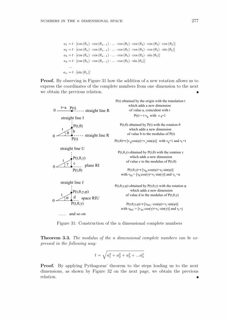
numbers in the n dimensional space 277
a1 = t · [cos (θn) · cos (θn−1) · ... · cos (θ5) · cos (θ4) · cos (θ3) · cos (θ2)]a2 = t · [cos (θn) · cos (θn−1) · ... · cos (θ5) · cos (θ4) · cos (θ3) · sin (θ2)]a3 = t · [cos (θn) · cos (θn−1) · ... · cos (θ5) · cos (θ4) · sin (θ3)]a4 = t · [cos (θn) · cos (θn−1) · ... · cos (θ5) · sin (θ4)]
...
an = t · [sin (θn)]
Proof. By observing in Figure 31 how the addition of a new rotation allows us toexpress the coordinates of the complete numbers from one dimension to the nextwe obtain the previous relation.
Figure 31: Construction of the n dimensional complete numbers
Theorem 3.3. The modulus of the n dimensional complete numbers can be ex-pressed in the following way:
t =√
a21 + a2
2 + a23 + ...a2
n
Proof. By applying Pythagoras’ theorem to the steps leading us to the nextdimensions, as shown by Figure 32 on the next page, we obtain the previousrelation.
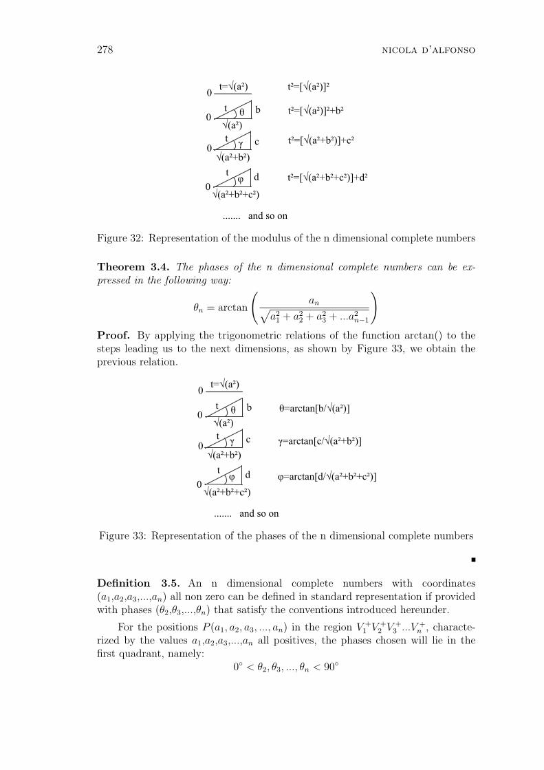
278 nicola d’alfonso
Figure 32: Representation of the modulus of the n dimensional complete numbers
Theorem 3.4. The phases of the n dimensional complete numbers can be ex-pressed in the following way:
θn = arctan
(an√
a21 + a2
2 + a23 + ...a2
n−1
)
Proof. By applying the trigonometric relations of the function arctan() to thesteps leading us to the next dimensions, as shown by Figure 33, we obtain theprevious relation.
Figure 33: Representation of the phases of the n dimensional complete numbers
Definition 3.5. An n dimensional complete numbers with coordinates(a1,a2,a3,...,an) all non zero can be defined in standard representation if providedwith phases (θ2,θ3,...,θn) that satisfy the conventions introduced hereunder.
For the positions P (a1, a2, a3, ..., an) in the region V +1 V +
2 V +3 ...V +
n , characte-rized by the values a1,a2,a3,...,an all positives, the phases chosen will lie in thefirst quadrant, namely:
0 < θ2, θ3, ..., θn < 90
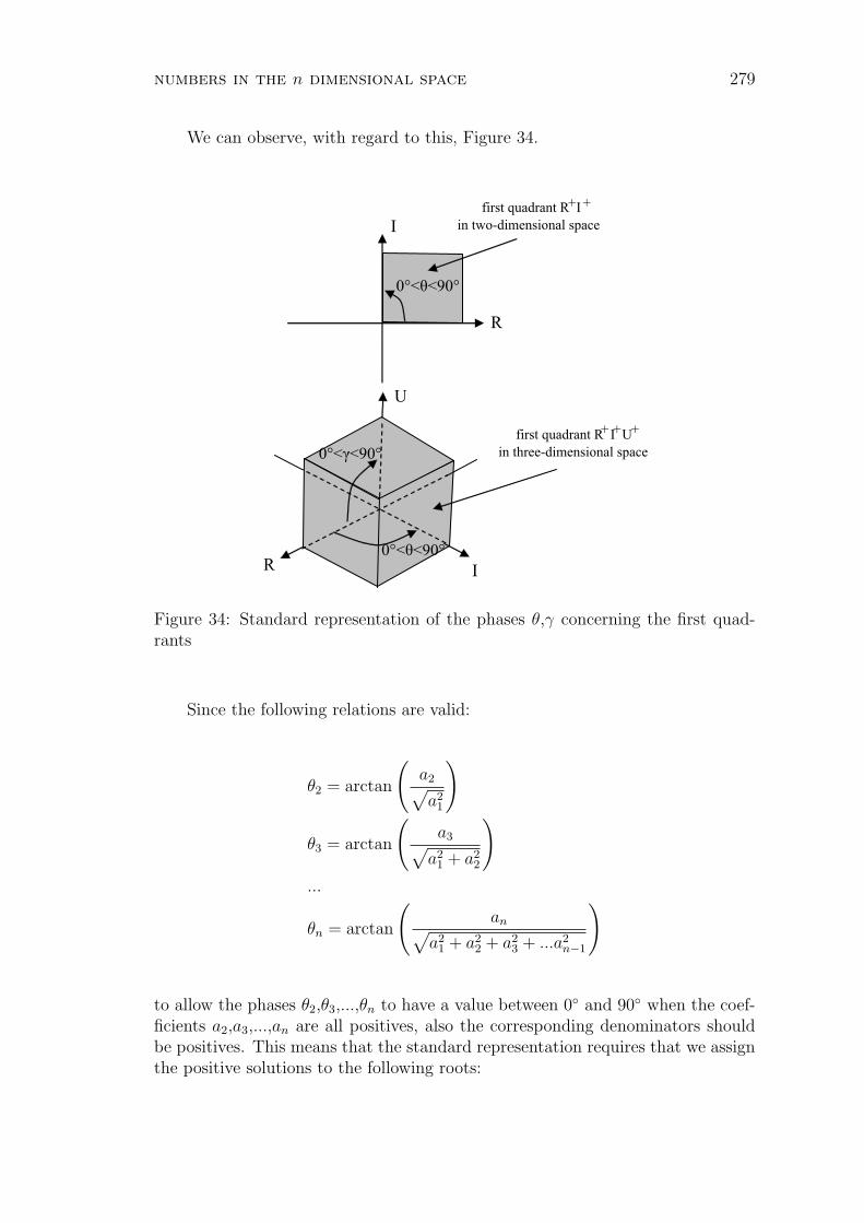
numbers in the n dimensional space 279
We can observe, with regard to this, Figure 34.
Figure 34: Standard representation of the phases θ,γ concerning the first quad-rants
Since the following relations are valid:
θ2 = arctan
(a2√a2
1
)
θ3 = arctan
(a3√
a21 + a2
2
)
...
θn = arctan
(an√
a21 + a2
2 + a23 + ...a2
n−1
)
to allow the phases θ2,θ3,...,θn to have a value between 0 and 90 when the coef-ficients a2,a3,...,an are all positives, also the corresponding denominators shouldbe positives. This means that the standard representation requires that we assignthe positive solutions to the following roots:
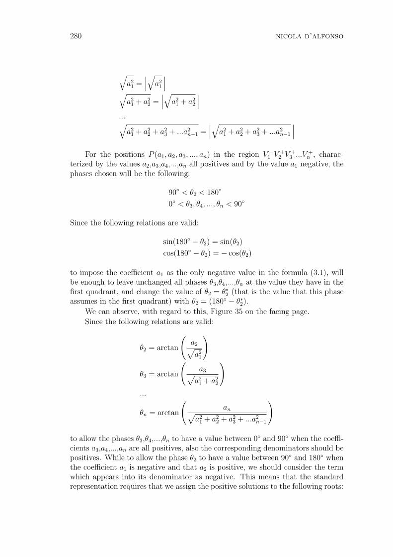
280 nicola d’alfonso
√a2
1 =∣∣∣√
a21
∣∣∣√
a21 + a2
2 =∣∣∣√
a21 + a2
2
∣∣∣...√
a21 + a2
2 + a23 + ...a2
n−1 =∣∣∣√
a21 + a2
2 + a23 + ...a2
n−1
∣∣∣
For the positions P (a1, a2, a3, ..., an) in the region V −1 V +
2 V +3 ...V +
n , charac-terized by the values a2,a3,a4,...,an all positives and by the value a1 negative, thephases chosen will be the following:
90 < θ2 < 180
0 < θ3, θ4, ..., θn < 90
Since the following relations are valid:
sin(180 − θ2) = sin(θ2)
cos(180 − θ2) = − cos(θ2)
to impose the coefficient a1 as the only negative value in the formula (3.1), willbe enough to leave unchanged all phases θ3,θ4,...,θn at the value they have in thefirst quadrant, and change the value of θ2 = θ∗2 (that is the value that this phaseassumes in the first quadrant) with θ2 = (180 − θ∗2).
We can observe, with regard to this, Figure 35 on the facing page.
Since the following relations are valid:
θ2 = arctan
(a2√a2
1
)
θ3 = arctan
(a3√
a21 + a2
2
)
...
θn = arctan
(an√
a21 + a2
2 + a23 + ...a2
n−1
)
to allow the phases θ3,θ4,...,θn to have a value between 0 and 90 when the coeffi-cients a3,a4,...,an are all positives, also the corresponding denominators should bepositives. While to allow the phase θ2 to have a value between 90 and 180 whenthe coefficient a1 is negative and that a2 is positive, we should consider the termwhich appears into its denominator as negative. This means that the standardrepresentation requires that we assign the positive solutions to the following roots:
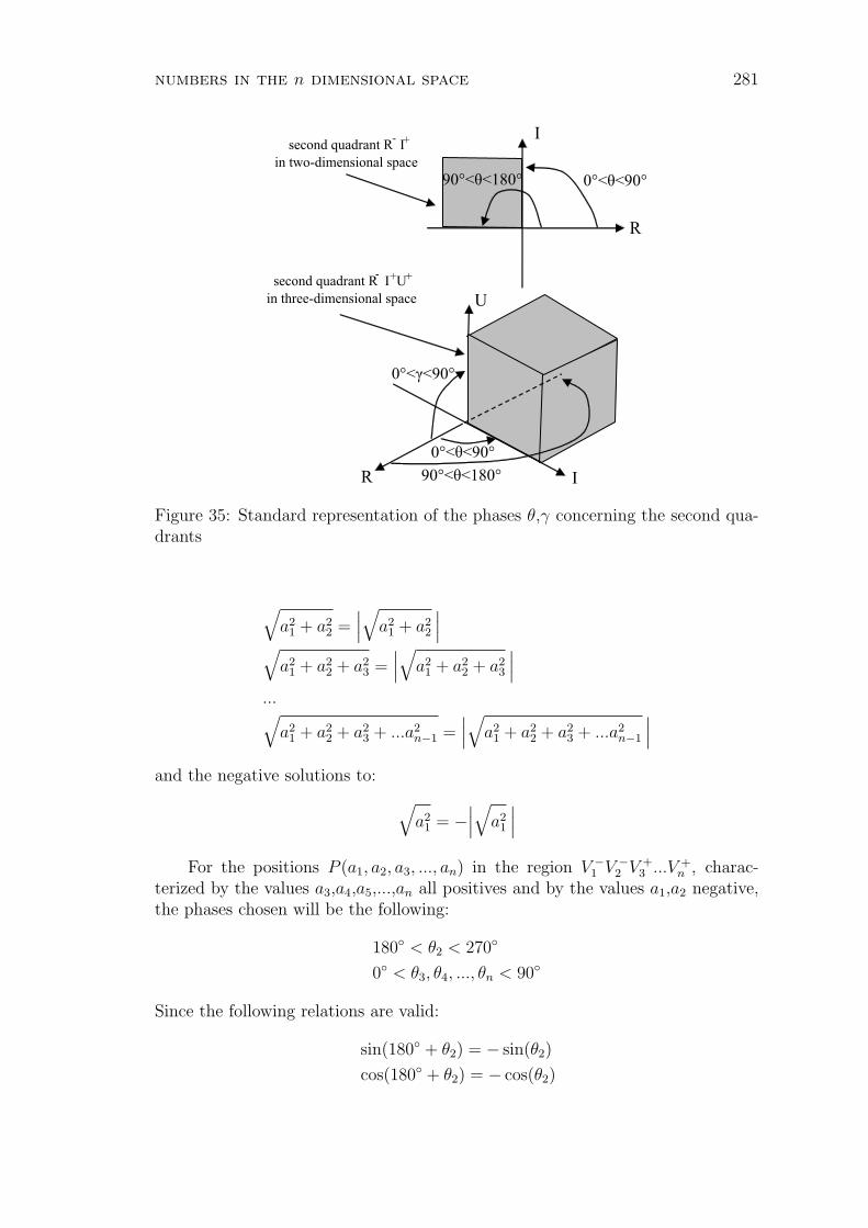
numbers in the n dimensional space 281
Figure 35: Standard representation of the phases θ,γ concerning the second qua-drants
√a2
1 + a22 =
∣∣∣√
a21 + a2
2
∣∣∣√
a21 + a2
2 + a23 =
∣∣∣√
a21 + a2
2 + a23
∣∣∣...√
a21 + a2
2 + a23 + ...a2
n−1 =∣∣∣√
a21 + a2
2 + a23 + ...a2
n−1
∣∣∣
and the negative solutions to:
√a2
1 = −∣∣∣√
a21
∣∣∣
For the positions P (a1, a2, a3, ..., an) in the region V −1 V −
2 V +3 ...V +
n , charac-terized by the values a3,a4,a5,...,an all positives and by the values a1,a2 negative,the phases chosen will be the following:
180 < θ2 < 270
0 < θ3, θ4, ..., θn < 90
Since the following relations are valid:
sin(180 + θ2) = − sin(θ2)
cos(180 + θ2) = − cos(θ2)
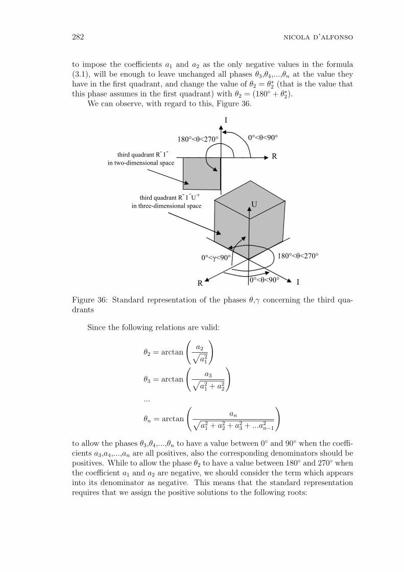
282 nicola d’alfonso
to impose the coefficients a1 and a2 as the only negative values in the formula(3.1), will be enough to leave unchanged all phases θ3,θ4,...,θn at the value theyhave in the first quadrant, and change the value of θ2 = θ∗2 (that is the value thatthis phase assumes in the first quadrant) with θ2 = (180 + θ∗2).
We can observe, with regard to this, Figure 36.
Figure 36: Standard representation of the phases θ,γ concerning the third qua-drants
Since the following relations are valid:
θ2 = arctan
(a2√a2
1
)
θ3 = arctan
(a3√
a21 + a2
2
)
...
θn = arctan
(an√
a21 + a2
2 + a23 + ...a2
n−1
)
to allow the phases θ3,θ4,...,θn to have a value between 0 and 90 when the coeffi-cients a3,a4,...,an are all positives, also the corresponding denominators should bepositives. While to allow the phase θ2 to have a value between 180 and 270 whenthe coefficient a1 and a2 are negative, we should consider the term which appearsinto its denominator as negative. This means that the standard representationrequires that we assign the positive solutions to the following roots:
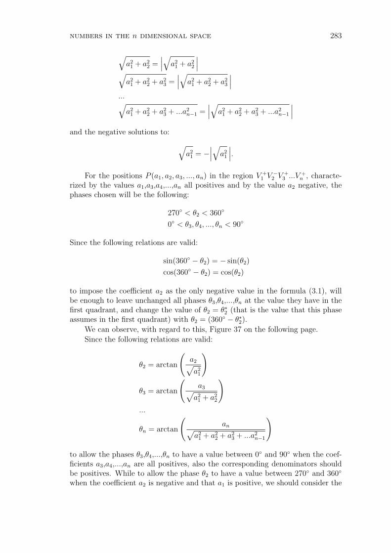
numbers in the n dimensional space 283
√a2
1 + a22 =
∣∣∣√
a21 + a2
2
∣∣∣√
a21 + a2
2 + a23 =
∣∣∣√
a21 + a2
2 + a23
∣∣∣...√
a21 + a2
2 + a23 + ...a2
n−1 =∣∣∣√
a21 + a2
2 + a23 + ...a2
n−1
∣∣∣
and the negative solutions to:
√a2
1 = −∣∣∣√
a21
∣∣∣.
For the positions P (a1, a2, a3, ..., an) in the region V +1 V −
2 V +3 ...V +
n , characte-rized by the values a1,a3,a4,...,an all positives and by the value a2 negative, thephases chosen will be the following:
270 < θ2 < 360
0 < θ3, θ4, ..., θn < 90
Since the following relations are valid:
sin(360 − θ2) = − sin(θ2)
cos(360 − θ2) = cos(θ2)
to impose the coefficient a2 as the only negative value in the formula (3.1), willbe enough to leave unchanged all phases θ3,θ4,...,θn at the value they have in thefirst quadrant, and change the value of θ2 = θ∗2 (that is the value that this phaseassumes in the first quadrant) with θ2 = (360 − θ∗2).
We can observe, with regard to this, Figure 37 on the following page.
Since the following relations are valid:
θ2 = arctan
(a2√a2
1
)
θ3 = arctan
(a3√
a21 + a2
2
)
...
θn = arctan
(an√
a21 + a2
2 + a23 + ...a2
n−1
)
to allow the phases θ3,θ4,...,θn to have a value between 0 and 90 when the coef-ficients a3,a4,...,an are all positives, also the corresponding denominators shouldbe positives. While to allow the phase θ2 to have a value between 270 and 360
when the coefficient a2 is negative and that a1 is positive, we should consider the
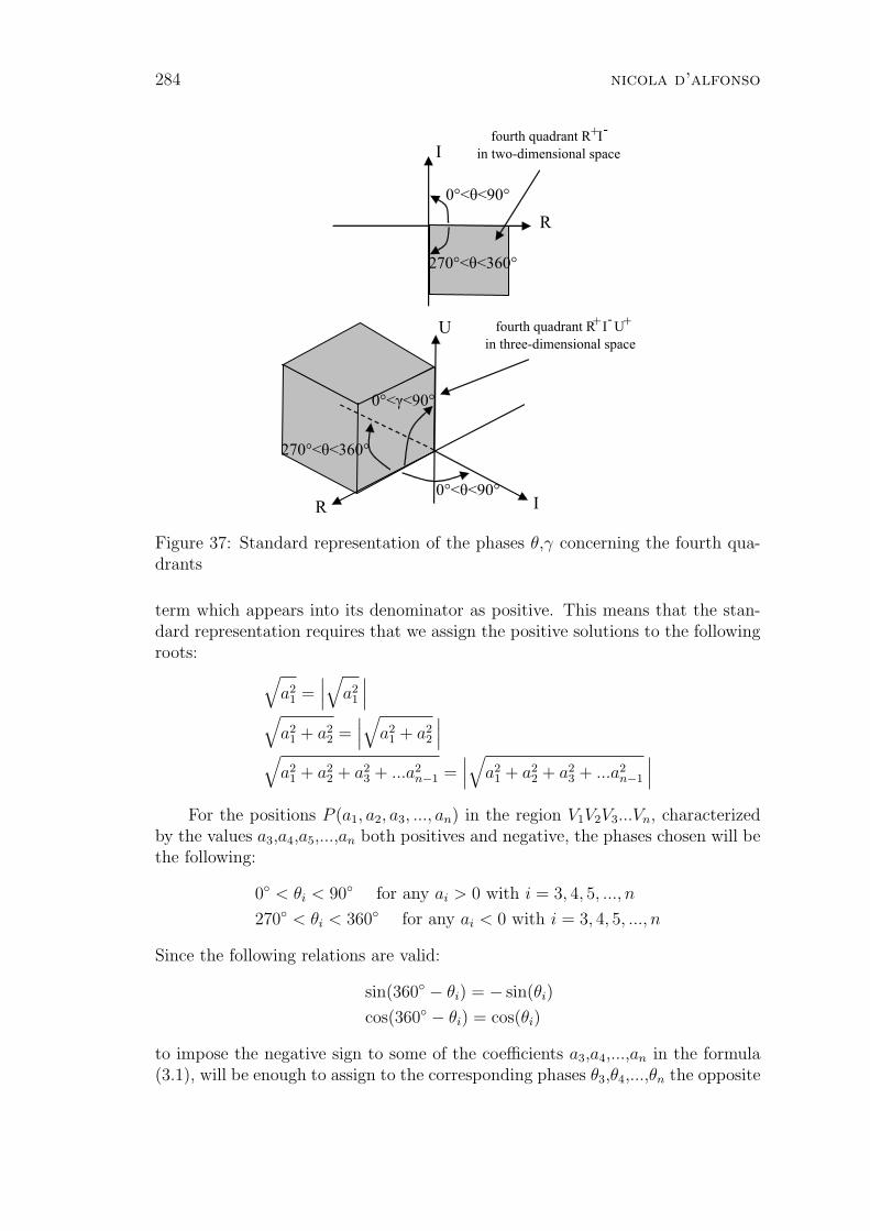
284 nicola d’alfonso
Figure 37: Standard representation of the phases θ,γ concerning the fourth qua-drants
term which appears into its denominator as positive. This means that the stan-dard representation requires that we assign the positive solutions to the followingroots:
√a2
1 =∣∣∣√
a21
∣∣∣√
a21 + a2
2 =∣∣∣√
a21 + a2
2
∣∣∣√
a21 + a2
2 + a23 + ...a2
n−1 =∣∣∣√
a21 + a2
2 + a23 + ...a2
n−1
∣∣∣
For the positions P (a1, a2, a3, ..., an) in the region V1V2V3...Vn, characterizedby the values a3,a4,a5,...,an both positives and negative, the phases chosen will bethe following:
0 < θi < 90 for any ai > 0 with i = 3, 4, 5, ..., n
270 < θi < 360 for any ai < 0 with i = 3, 4, 5, ..., n
Since the following relations are valid:
sin(360 − θi) = − sin(θi)
cos(360 − θi) = cos(θi)
to impose the negative sign to some of the coefficients a3,a4,...,an in the formula(3.1), will be enough to assign to the corresponding phases θ3,θ4,...,θn the opposite
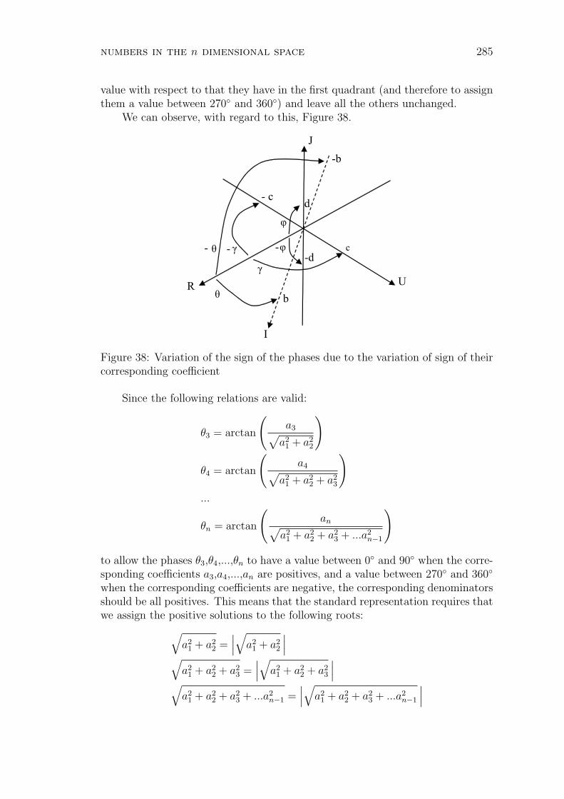
numbers in the n dimensional space 285
value with respect to that they have in the first quadrant (and therefore to assignthem a value between 270 and 360) and leave all the others unchanged.
We can observe, with regard to this, Figure 38.
Figure 38: Variation of the sign of the phases due to the variation of sign of theircorresponding coefficient
Since the following relations are valid:
θ3 = arctan
(a3√
a21 + a2
2
)
θ4 = arctan
(a4√
a21 + a2
2 + a23
)
...
θn = arctan
(an√
a21 + a2
2 + a23 + ...a2
n−1
)
to allow the phases θ3,θ4,...,θn to have a value between 0 and 90 when the corre-sponding coefficients a3,a4,...,an are positives, and a value between 270 and 360
when the corresponding coefficients are negative, the corresponding denominatorsshould be all positives. This means that the standard representation requires thatwe assign the positive solutions to the following roots:
√a2
1 + a22 =
∣∣∣√
a21 + a2
2
∣∣∣√
a21 + a2
2 + a23 =
∣∣∣√
a21 + a2
2 + a23
∣∣∣√
a21 + a2
2 + a23 + ...a2
n−1 =∣∣∣√
a21 + a2
2 + a23 + ...a2
n−1
∣∣∣

286 nicola d’alfonso
Since the management of sign of the coefficients a3,a4,...,an does not interferewith the angle θ2, we can combine it with the management of signs of a1 and a2
according to the manner described above.
Theorem 3.6. The standard representation of a n dimensional complete numberof coordinates (a1,a2,a3,...,an) all non zero requires to give the following solutionsto the following algebraic roots:√
a21 = a1√
a21 + a2
2 =∣∣∣√
a21 + a2
2
∣∣∣√
a21 + a2
2 + a23 =
∣∣∣√
a21 + a2
2 + a23
∣∣∣...√
a21 + a2
2 + a23 + ...a2
n−1 =∣∣∣√
a21 + a2
2 + a23 + ...a2
n−1
∣∣∣
Proof. In the case of the representations previously examined the phases assumethe values provided by the formulas:
θ2 = arctan
(a2√a2
1
)
θ3 = arctan
(a3√
a21 + a2
2
)
...
θn = arctan
(an√
a21 + a2
2 + a23 + ...a2
n−1
)
when we give to the algebraic roots involved just the values considered here. Andthis immediately proves the thesis.
For example in the four dimensional space the complete number with theexpression:
o(t, θ, γ, ϕ) = [cos (ϕ) · cos (γ) · cos (θ)] + i · [cos (ϕ) · cos (γ) · sin (θ)]
+ u · [cos (ϕ) · sin (γ)] + j · [sin (ϕ)]
associated to the position:
o(a, b, c, d) = o(−1, 1,−1, 1)
could be expressed in standard representation through the following phases:
θ = arctan( b
a
)= arctan
( 1
−1
)= 135
γ = arctan( c
|√a2 + b2 |)
= arctan(−1√
2
)' −35.26
ϕ = arctan( d
|√a2 + b2 + c2 |)
= arctan( 1√
3
)= 30

numbers in the n dimensional space 287
and the following modulus:
t =√
a2 + b2 + c2 + d2 =√
4 = 2
To verify that the standard representation o(θ, γ, ϕ) thus obtained identifies justthe position o(−1, 0, 1, 0) it is sufficient to perform the following calculations:
a = t · cos (ϕ) · cos (γ) · cos (θ) = 2 · cos (30) · cos (' −35.26) · cos (135) = −1b = t · cos (ϕ) · cos (γ) · sin (θ) = 2 · cos (30) · cos (' −35.26) · sin (135) = 1c = t · cos (ϕ) · sin (γ) = 2 · cos (30) · sin (' −35.26) = −1d = t · sin (ϕ) = 2 · sin (30) = 1
Definition 3.7. An n dimensional complete numbers with coordinates(a1,a2,a3,...,an) all non zero can be defined in complementary representation ifprovided with phases obtained by the values: θ2,θ3,...,θn of the standard represen-tation through those substitutions which allow us to identify the same positions.
Theorem 3.8. If we call θ2,θ3,...,θn the phases that allow to an n dimensionalcomplete number provided with coordinates (a1,a2,a3,...,an) all non zero and instandard representation to identify any position of the space V1V2V3...Vn, the al-ternative sets of phases able to individuate the same position can be obtained bythe following values: θ, (360 − θ), (180 − θ), (θ + 180).
Proof. The ability to express through the formula (3.1) the same positions of thestandard representation, assigning to the phases the following values: θ, (360−θ),(180−θ), (θ+180) comes from the fact that in this way we maintain the moduliunchanged and introduce signs which can neutralize each other, as shown by thefollowing relations:
cos (θ) = cos (θ)
sin (θ) = sin (θ)
cos (360 − θ) = cos (θ)
sin (360 − θ) = − sin (θ)
cos (180 − θ) = − cos (θ)
sin (180 − θ) = sin (θ)
cos (θ + 180) = − cos (θ)
sin (θ + 180) = − sin (θ)
Using this process it is possible to combine, for example, the standard represen-tation concerning the fourth dimension:
o(t, θ, γ, ϕ) = [cos (ϕ) · cos (γ) · cos (θ)] + i · [cos (ϕ) · cos (γ) · sin (θ)]
+ u · [cos (ϕ) · sin (γ)] + j · [sin (ϕ)]
to the following complementary representations:

288 nicola d’alfonso
o(t, θ, γ + 180, 180 − ϕ) = [cos (180 − ϕ) · cos (γ + 180) · cos (θ)]+ i · [cos (180 − ϕ) · cos (γ + 180) · sin (θ)]+ u · [cos (180 − ϕ) · sin (γ + 180)]+ j · [sin (180 − ϕ)]
o(t, θ + 180, 360 − γ, 180 − ϕ) = [cos (180 − ϕ) · cos (360 − γ) · cos (θ + 180)]+ i · [cos (180 − ϕ) · cos (360 − γ) · sin (θ + 180)]+ u · [cos (180 − ϕ) · sin (360 − γ)]+ j · [sin (180 − ϕ)]
o(t, θ + 180, 180 − γ, ϕ) = [cos (ϕ) · cos (180 − γ) · cos (θ + 180)]+ i · [cos (ϕ) · cos (180 − γ) · sin (θ + 180)]+ u · [cos (ϕ) · sin (180 − γ)]+ j · [sin (ϕ)]
For example if you want to identify a complementary representation of thefollowing four dimensional complete number:
o(a, b, c, d) = o(−1, 1,−1, 1)
whose standard representation is provided with the following phases:
θ∗ = 135
γ∗ ' −35.26
ϕ∗ = 30
and the following modulus:t = 2
it is sufficient to perform the following calculations:
θ = θ∗ = 135
γ = γ∗ + 180 ' (' −35.26) + 180 ' 144.74
ϕ = 180 − ϕ∗ = 180 − 30 = 150
To verify that the complementary representation o(θ, γ, ϕ) thus obtained identifiesjust the position o(−1, 1,−1, 1) it is sufficient to perform the following calcula-tions:
a = t · cos (ϕ) · cos (γ) · cos (θ) = 2 · cos (150) · cos (' 144.74) · cos (135) = −1b = t · cos (ϕ) · cos (γ) · sin (θ) = 2 · cos (150) · cos (' 144.74) · sin (135) = 1c = t · cos (ϕ) · sin (γ) = 2 · cos (150) · sin (' 144.74) = −1d = t · sin (ϕ) = 2 · sin (150) = 1

numbers in the n dimensional space 289
Definition 3.9. The n dimensional complete numbers with coordinates(a1,a2,a3,...,an) some of which are zero can be defined in standard representa-tion if their phases besides to be consistent with those of the other standardrepresentations (according to the definition 3.5) assume the zero value in case ofindetermination.
The relations that give the values of the phases for the standard representationare the following:
θ2 = arctan(a2
a1
)
θ3 = arctan
(a3
|√
a21 + a2
2 |
)
θ3 = arctan
(a4
|√
a21 + a2
2 + a23 |
)
...
θn = arctan
(an
|√a21 + a2
2 + a23 + ...a2
n−1 |
)
Due to coefficients with zero value, we can have the following notable cases:
θ2 = arctan( 0
a1
)=
0 for a1 > 0
180 for a1 < 0
θi = arctan(ai
0
)=
90 for ai > 0
270 for ai < 0
θi = arctan
(0
|x 6= 0|)
= 0
θi = arctan(0
0
)= 0
For example in the four dimensional space the complete number with expression:
o(t, θ, γ, ϕ) =[cos (ϕ) · cos (γ) · cos (θ)] + i · [cos (ϕ) · cos (γ) · sin (θ)]
+ u · [cos (ϕ) · sin (γ)] + j · [sin (ϕ)]
associated to the position:
o(a, b, c, d) = o(−1, 0, 1, 0)
could be expressed in standard representation through the following phases:
θ = arctan( b
a
)= arctan
( 0
−1
)= 180
γ = arctan( c
|√a2 + b2 |)
= arctan(1
1
)= 45
ϕ = arctan( d
|√a2 + b2 + c2 |)
= arctan( 0√
2
)= 0
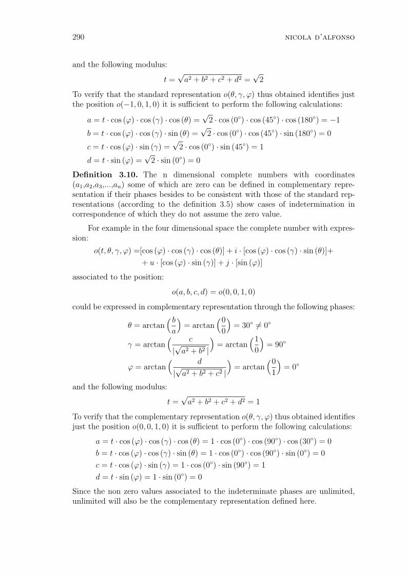
290 nicola d’alfonso
and the following modulus:
t =√
a2 + b2 + c2 + d2 =√
2
To verify that the standard representation o(θ, γ, ϕ) thus obtained identifies justthe position o(−1, 0, 1, 0) it is sufficient to perform the following calculations:
a = t · cos (ϕ) · cos (γ) · cos (θ) =√
2 · cos (0) · cos (45) · cos (180) = −1
b = t · cos (ϕ) · cos (γ) · sin (θ) =√
2 · cos (0) · cos (45) · sin (180) = 0
c = t · cos (ϕ) · sin (γ) =√
2 · cos (0) · sin (45) = 1
d = t · sin (ϕ) =√
2 · sin (0) = 0
Definition 3.10. The n dimensional complete numbers with coordinates(a1,a2,a3,...,an) some of which are zero can be defined in complementary repre-sentation if their phases besides to be consistent with those of the standard rep-resentations (according to the definition 3.5) show cases of indetermination incorrespondence of which they do not assume the zero value.
For example in the four dimensional space the complete number with expres-sion:
o(t, θ, γ, ϕ) =[cos (ϕ) · cos (γ) · cos (θ)] + i · [cos (ϕ) · cos (γ) · sin (θ)]+
+ u · [cos (ϕ) · sin (γ)] + j · [sin (ϕ)]
associated to the position:
o(a, b, c, d) = o(0, 0, 1, 0)
could be expressed in complementary representation through the following phases:
θ = arctan( b
a
)= arctan
(0
0
)= 30 6= 0
γ = arctan( c
|√a2 + b2 |)
= arctan(1
0
)= 90
ϕ = arctan( d
|√a2 + b2 + c2 |)
= arctan(0
1
)= 0
and the following modulus:
t =√
a2 + b2 + c2 + d2 = 1
To verify that the complementary representation o(θ, γ, ϕ) thus obtained identifiesjust the position o(0, 0, 1, 0) it is sufficient to perform the following calculations:
a = t · cos (ϕ) · cos (γ) · cos (θ) = 1 · cos (0) · cos (90) · cos (30) = 0
b = t · cos (ϕ) · cos (γ) · sin (θ) = 1 · cos (0) · cos (90) · sin (0) = 0
c = t · cos (ϕ) · sin (γ) = 1 · cos (0) · sin (90) = 1
d = t · sin (ϕ) = 1 · sin (0) = 0
Since the non zero values associated to the indeterminate phases are unlimited,unlimited will also be the complementary representation defined here.
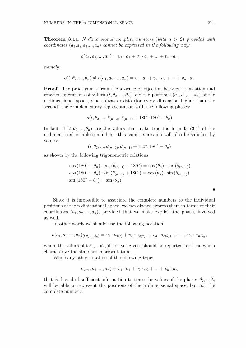
numbers in the n dimensional space 291
Theorem 3.11. N dimensional complete numbers (with n > 2) provided withcoordinates (a1,a2,a3,...,an) cannot be expressed in the following way:
o(a1, a2, ..., an) = v1 · a1 + v2 · a2 + ... + vn · an
namely:
o(t, θ2, ..., θn) 6= o(a1, a2, ..., an) = v1 · a1 + v2 · a2 + ... + vn · an
Proof. The proof comes from the absence of bijection between translation androtation operations of values (t, θ2, ..., θn) and the positions (a1, a2, ..., an) of then dimensional space, since always exists (for every dimension higher than thesecond) the complementary representation with the following phases:
o(t, θ2, ..., θ(n−2), θ(n−1) + 180, 180 − θn)
In fact, if (t, θ2, ..., θn) are the values that make true the formula (3.1) of then dimensional complete numbers, this same expression will also be satisfied byvalues:
(t, θ2, ..., θ(n−2), θ(n−1) + 180, 180 − θn)
as shown by the following trigonometric relations:
cos (180 − θn) · cos (θ(n−1) + 180) = cos (θn) · cos (θ(n−1))
cos (180 − θn) · sin (θ(n−1) + 180) = cos (θn) · sin (θ(n−1))
sin (180 − θn) = sin (θn)
Since it is impossible to associate the complete numbers to the individualpositions of the n dimensional space, we can always express them in terms of theircoordinates (a1, a2, ..., an), provided that we make explicit the phases involvedas well.
In other words we should use the following notation:
o(a1, a2, ..., an)(t,θ2,...,θn) = v1 · a1(t) + v2 · a2(θ2) + v3 · a3(θ3) + ... + vn · an(θn)
where the values of t,θ2,...,θn, if not yet given, should be reported to those whichcharacterize the standard representation.
While any other notation of the following type:
o(a1, a2, ..., an) = v1 · a1 + v2 · a2 + ... + vn · an
that is devoid of sufficient information to trace the values of the phases θ2,...,θn
will be able to represent the positions of the n dimensional space, but not thecomplete numbers.

292 nicola d’alfonso
3.2. N dimensional operations
Definition 3.12. In the space V1V2V3...Vn we can define addition betweentwo positions o(a11, a21, ..., an1) and o(a12, a22, ..., an2) as the positiono(a1(1+2), a2(1+2), ..., an(1+2)) represented also with the symbol o(a11, a21, ..., an1) +o(a12, a22, ..., an2) that satisfies the following condition:
o1+2(a1(1+2), a2(1+2), ..., an(1+2)) = o1+2(a11 + a12, a11 + a12, ..., an1 + an2)
This condition is equivalent to take the position of the space V1V2V3...Vn
provided with the following coordinates:
a1(1+2) = a11 + a12
a2(1+2) = a21 + a22
...
an(1+2) = an1 + an2
For example in the fourth dimension we have:
o1+2(a1+2, b1+2, c1+2, d1+2) = o1+2(a1 + a2, b1 + b2, c1 + c2, d1 + d2)
with:
a1+2 = a1 + a2
b1+2 = b1 + b2
c1+2 = c1 + c2
d1+2 = d1 + d2
It should be emphasized that the addition must be considered an operationthat works on the positions and not on the complete numbers, at least for everydimension higher than the second, for which there is no bijection between thepositions and the complete numbers.
To integrate the operation of addition, working on the positions, with theothers, working on the complete numbers, will be enough making reference tothe complete number that we can obtain assigning to the sum the phases of thestandard representation.
Theorem 3.13. The properties embodied by Theorems 2.21, 2.22, 2.23, 2.24 forthe third dimension remain valid for the next dimensions as well.
Proof. In practise, the proofs of these theorems can be merely extended to anumber of dimensions at will, since each coordinate is treated independently ofthe others, and has the same properties.
Definition 3.14. In the space V1V2V3...Vn we can define subtraction between twopositions o(a11, a21, ..., an1) and o(a12, a22, ..., an2) as the position o(a1(1−2), a2(1−2), ...,an(1−2)) represented also with the symbol o(a11, a21, ..., an1)−o(a12, a22, ..., an2) thatsatisfies the following condition:
o1−2(a1(1−2), a2(1−2), ..., an(1−2)) + o(a12, a22, ..., an2) = o(a11, a21, ..., an1)
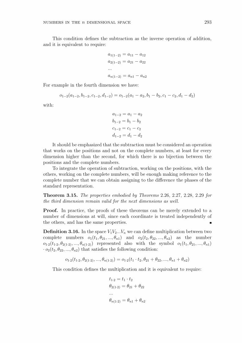
numbers in the n dimensional space 293
This condition defines the subtraction as the inverse operation of addition,and it is equivalent to require:
a1(1−2) = a11 − a12
a2(1−2) = a21 − a22
...
an(1−2) = an1 − an2
For example in the fourth dimension we have:
o1−2(a1−2, b1−2, c1−2, d1−2) = o1−2(a1 − a2, b1 − b2, c1 − c2, d1 − d2)
with:
a1−2 = a1 − a2
b1−2 = b1 − b2
c1−2 = c1 − c2
d1−2 = d1 − d2
It should be emphasized that the subtraction must be considered an operationthat works on the positions and not on the complete numbers, at least for everydimension higher than the second, for which there is no bijection between thepositions and the complete numbers.
To integrate the operation of subtraction, working on the positions, with theothers, working on the complete numbers, will be enough making reference to thecomplete number that we can obtain assigning to the difference the phases of thestandard representation.
Theorem 3.15. The properties embodied by Theorems 2.26, 2.27, 2.28, 2.29 forthe third dimension remain valid for the next dimensions as well.
Proof. In practice, the proofs of these theorems can be merely extended to anumber of dimensions at will, since each coordinate is treated independently ofthe others, and has the same properties.
Definition 3.16. In the space V1V2...Vn we can define multiplication between twocomplete numbers o1(t1, θ21, ..., θn1) and o2(t2, θ22, ..., θn2) as the numbero1·2(t1·2, θ2(1·2), ..., θn(1·2)) represented also with the symbol o1(t1, θ21, ..., θn1)· o2(t2, θ22, ..., θn2) that satisfies the following condition:
o1·2(t1·2, θ2(1·2), ..., θn(1·2)) = o1·2(t1 · t2, θ21 + θ22, ..., θn1 + θn2)
This condition defines the multiplication and it is equivalent to require:
t1·2 = t1 · t2θ2(1·2) = θ21 + θ22
...
θn(1·2) = θn1 + θn2
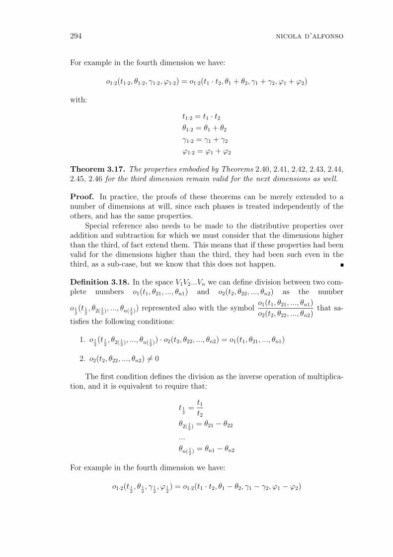
294 nicola d’alfonso
For example in the fourth dimension we have:
o1·2(t1·2, θ1·2, γ1·2, ϕ1·2) = o1·2(t1 · t2, θ1 + θ2, γ1 + γ2, ϕ1 + ϕ2)
with:
t1·2 = t1 · t2θ1·2 = θ1 + θ2
γ1·2 = γ1 + γ2
ϕ1·2 = ϕ1 + ϕ2
Theorem 3.17. The properties embodied by Theorems 2.40, 2.41, 2.42, 2.43, 2.44,2.45, 2.46 for the third dimension remain valid for the next dimensions as well.
Proof. In practice, the proofs of these theorems can be merely extended to anumber of dimensions at will, since each phases is treated independently of theothers, and has the same properties.
Special reference also needs to be made to the distributive properties overaddition and subtraction for which we must consider that the dimensions higherthan the third, of fact extend them. This means that if these properties had beenvalid for the dimensions higher than the third, they had been such even in thethird, as a sub-case, but we know that this does not happen.
Definition 3.18. In the space V1V2...Vn we can define division between two com-plete numbers o1(t1, θ21, ..., θn1) and o2(t2, θ22, ..., θn2) as the number
o 12(t 1
2, θ2( 1
2), ..., θn( 1
2)) represented also with the symbol
o1(t1, θ21, ..., θn1)
o2(t2, θ22, ..., θn2)that sa-
tisfies the following conditions:
1. o 12(t 1
2, θ2( 1
2), ..., θn( 1
2)) · o2(t2, θ22, ..., θn2) = o1(t1, θ21, ..., θn1)
2. o2(t2, θ22, ..., θn2) 6= 0
The first condition defines the division as the inverse operation of multiplica-tion, and it is equivalent to require that:
t 12
=t1t2
θ2( 12) = θ21 − θ22
...
θn( 12) = θn1 − θn2
For example in the fourth dimension we have:
o1·2(t 12, θ 1
2, γ 1
2, ϕ 1
2) = o1·2(t1 · t2, θ1 − θ2, γ1 − γ2, ϕ1 − ϕ2)
numbers in the n dimensional space 295
with:
t 12
=t1t2
θ 12
= θ1 − θ2
γ 12
= γ1 − γ2
ϕ 12
= ϕ1 − ϕ2
The second condition gets its own justification by the necessity of defining thedivisions in an univocal way. In fact when that condition is not valid, the expres-sion:
o 12(t 1
2, θ2( 1
2), ..., θn( 1
2)) · 0 = 0
besides to require a zero dividend o1(t1, θ21, ..., θn1) as well, would be satisfied bymore values of o 1
2(t 1
2, θ2( 1
2), ..., θn( 1
2)).
Theorem 3.19. The properties embodied by Theorems 2.57,2.58,2.59, 2.60, 2.61,2.62, 2.63 for the third dimension remain valid for the next dimensions as well.
Proof. In practice, the proofs of these theorems can be merely extended to anumber of dimensions at will, since each phases is treated independently of theothers, and has the same properties.
Special reference also needs to be made to the distributive properties overaddition and subtraction for which we must consider that the dimensions higherthan the third, of fact extend them. This means that if these properties had beenvalid for the dimensions higher than the third, they had been such even in thethird, as a sub-case, but we know that this does not happen.
Definition 3.20. In the space V1V2...Vn we can define n-th power of the completenumber o(t, θ2, ..., θi) with n (natural number) known as exponent and o(t, θ2, ..., θi)known as base, as the number o↑n(t↑n, θ2(↑n), ..., θi(↑n)) also represented with thesymbol o(t, θ2, ..., θi)
n that satisfies the following conditions:
1. o(t, θ2, ..., θi)n = o(t, θ2, ..., θi) · ... · o(t, θ2, ..., θi) for n > 0
2. o(t, θ2, ..., θi)n = o(t,θ2,...,θi)
o(t,θ2,...,θi)= 1 for n = 0
3. o(t, θ2, ..., θi)n =
1
o(t, θ2, ..., θi)
. . .
o(t, θ2, ..., θi)
for n < 0
4. n > 0 for o(t, θ2, ..., θi) = 0
We note that the term o(t, θ2, ..., θi) in the first and third conditions is intendedto appear |n| times.
296 nicola d’alfonso
The first condition defines the repeated multiplication of the base by itself apositive number of times, the second a zero number of times, and finally the thirda negative number of times. All these conditions correspond to require:
t↑n = tn
θ2(↑n) = θ2 · n...
θi(↑n) = θi · n
For example in the fourth dimension we have:
o↑n(t, θ, γ, ϕ)n = o↑n(t↑n, θ↑n, γ↑n, ϕ↑n)
with:
t↑n = tn
θ↑n = θ · nγ↑n = γ · nϕ↑n = ϕ · n
The fourth condition gets its own justification by the impossibility of definingthe n-th power module when to be multiplied by itself a zero number or a negativenumber of times is just the 0, because in this case would be present the followingdivisions for 0:
o(t, θ2, ..., θi)n =
0
0= 1 for n = 0
o(t, θ2, ..., θi)n =
1
0
. . .
0
for n < 0 with 0 that appears —n— times
Theorem 3.21. The properties embodied by Theorems 2.65, 2.66, 2.67, 2.68, 2.69for the third dimension remain valid for the next dimensions as well.
Proof. In practice, the proofs of these theorems can be repeated unchanged fordimensions higher than the third, since they do not depend on the number ofdimensions considered but on the structure of the n-th power.
Definition 3.22. In the space V1V2...Vn we can define n-th root of the completenumber o(t, θ2, ..., θi) with n (natural number) known as degree and o(t, θ2, ..., θi)known as radicand, as the number o↓n(t↓n, θ2(↓n), ..., θi(↓n)) also represented with
the symbol n√
o(t, θ2, ..., θi) that satisfies the following conditions:
numbers in the n dimensional space 297
1. n√
o(t, θ2, ..., θi) · ... · n√
o(t, θ2, ..., θi) = o(t, θ2, ..., θi) for n > 0
2.1
n√
o(t, θ2, ..., θi)
...n√
o(t, θ2, ..., θi)
= o(t, θ2, ..., θi) for n < 0
3. θ2(↓n) = θ2
n, θ3(↓n) = θ3
n, ..., θi(↓n) = θi
n
4. n 6= 0 for any o(t, θ2, ..., θi)
5. n ≥ 0 for o(t, θ2, ..., θi) = 0
6. n√
t > 0, t > 0
We note that the term n√
o(t, θ2, ..., θi) in the first and second conditions is intendedto appear |n| times.
The first condition defines the repeated multiplication of the root by itselfa positive number of times, while the second a negative number of times. Boththese conditions correspond to require:
t↓n =n√
t
θ2(↓n) =θ2 + k · 360
nfor k = ±1,±2,±3,±4, ...
...
θi(↓n) =θi + k · 360
nfor k = ±1,±2,±3,±4, ...
The third condition gets its own justification by the necessity of defining then-th root in an univocal way. In fact, when that condition is not valid, thereare n(i−1) different complete numbers able to satisfy this definition: one for eachdistinct set of phases θ2(↓n),θ3(↓n),..., θi(↓n) given by the relations seen above.
For example in the fourth dimension we have:
n√
o(t, θ, γ, ϕ) = o↓n(t↓n, θ↓n, γ↓n, ϕ↓n)
with:
t↓n =n√
t
θ↓n =θ
n
γ↓n =γ
n
ϕ↓n =ϕ
n
298 nicola d’alfonso
Also the fourth condition gets its own justification by the necessity of definingthe n-th root in an univocal way. In fact when that condition is not valid, themultiplication of the root by itself a number of times equal to 0 would require theuse of the following expression:
n√
o(t, θ2, ..., θi)n√
o(t, θ2, ..., θi)= 1
that would be satisfied by several values of n√
[o(t, θ2, ..., θi)].The fifth condition gets its own justification by the impossibility of defining
values of n-th root that multiplied by itself a negative number of times are ableto give as the result just 0 value. In fact the following expression:
1n√
o(t, θ2, ..., θi)
...n√
o(t, θ2, ..., θi)
= 0 for n < 0, n√
o(t, θ2, ..., θi) appears —n— times
requires the existence of a divisor of 1 that can assign to it a quotient equal to 0:a thing that we know impossible.
The sixth condition gets its own justification by the need to make acceptablethe n-th root in regard the modulus t of the complete number o(t, θ2, ..., θi).
Theorem 3.23. The properties embodied by Theorems 2.71, 2.72, 2.73 for thethird dimension remain valid for the next dimensions as well.
Proof. In practice, the proofs of these theorems can be repeated unchanged fordimensions higher than the third, since they do not depend on the number ofdimensions considered but on the structure of the n-th root.
Definition 3.24. In the space V1V2...Vn we can define power with rational expo-
nentm
n(n,m both natural numbers) of the complete number o(t, θ2, ..., θi) with
m
nknown as the rational exponent and o(t, θ2, ..., θi) known as base, as the number
o↑m↓n(t↑m↓n, θ2(↑m↓n), .., θi(↑m↓n)) also represented with the symbol o(t, θ2, .., θi)mn or
n√
o(t, θ2, ..., θi)m that satisfies the following conditions:
1.[
n√
o(t, θ2, ..., θi)m
]n
= o(t, θ2, ..., θi)m
2. m > 0 for o(t, θ2, ..., θi) = 0
3. n 6= 0 for any o(t, θ2, ..., θi)m and therefore for any o(t, θ2, ..., θi)
4. n ≥ 0 for o(t, θ2, ..., θi)m = 0 and therefore for o(t, θ2, ..., θi) = 0

numbers in the n dimensional space 299
5. θ2(↑m↓n) =θ2 ·m
n, θ3(↑m↓n) =
θ3 ·mn
, ..., θi(↑m↓n) =θi ·m
n
6. n√
tm > 0, tm > 0
7. n√
t > 0, t > 0
The first condition defines the power with rational exponent as a n-th rootof a m-th power.
The second condition is required for the correct definition of the m-th power.The third, the fourth, the fifth and the sixth conditions are required for the
correct definition of n-th root.
For example in the fourth dimension we have:
n
√o(t, θ, γ, ϕ)m = o↑m↓n(t↑m↓n, θ↑m↓n, γ↑m↓n, ϕ↑m↓n)
with:
t↓n = tmn
θ↓n =m
n· θ
γ↓n =m
n· γ
ϕ↓n =m
n· ϕ
The seventh condition is required to make possible the reversal of the orderbetween root and power, namely to write:
[n√
o(t, θ2, ..., θi)]m
and therefore:
(n√
t )m
Theorem 3.25. The properties embodied by Theorems 2.75, 2.76, 2.77, 2.78, 2.79,2.80, 2.81 for the third dimension remain valid for the next dimensions as well.
Proof. In practice, the proofs of these theorems can be repeated unchanged fordimensions higher than the third, since they do not depend on the number ofdimensions considered but on the structure of the power with rational exponent.
300 nicola d’alfonso
References
[1] Hardy, G.H., A course of pure mathematics. Centenary edition. Reprintof the tenth (1952) edition with a foreword by T.W. Korner. CambridgeUniversity Press, Cambridge, 2008. xx+509 pp. ISBN: 978-0-521-72055-7MR2400109
Accepted: 28.05.2011
italian journal of pure and applied mathematics – n. 29−2012 (301−308) 301
A RADICAL PROPERTY OF HYPERRINGS
A. Asokkumar
M. Velrajan
Department of MathematicsAditanar College of Arts and ScienceTiruchendur – 628216, TamilnaduIndiae-mail: ashok [email protected]
Abstract. In this paper we prove that Von Neumann regularity is a radical propertyon hyperrings.
Keywords and phrases: Hyperring, Regular hyperring, Hyperideal, Hyperradical,Radical Property.2000 AMS Subject Classification Codes: 20N20.
1. Introduction
The theory of hyperstructures was introduced in 1934 by Marty [11] at the 8th Con-gress of Scandinavian Mathematicians. This theory has been subsequently deve-loped by Corsini [5], [6], Mittas [12], [13], Stratigopoulos [17], Vougiouklis [20] andby various authors. Basic definitions and propositions about the hyperstructuresare found in [5], [6] and [20]. Krasner [10] has studied the notion of hyperfields,hyperrings and then many researchers like Davvaz [7], Massouros [14] and othersfollowed him.
There are different notions of hyperrings (R, +, ·). If in a hyperring the ad-dition + is a hyperoperation and the multiplication · is a binary operation, thenthe hyperring is called a Krasner (additive) hyperring [10]. The monograph [8]of Davvaz and Leoreanu-Fotea contains many results about various hyperrings.Asokkumar and Velrajan [1], [4] have studied Von Neumann regularity in Krasnerhyperrings. Rota [16] introduced multiplicative hyperrings, where the additionsare binary operations and multiplications are hyperoperations. De Salvo [9] in-troduced hyperrings in which the additions and the multiplications are hyperop-erations. These hyperrings are studied by Rahnamani Barghi [15] and also byAsokkumar and Velrajan [2], [3], [19].
302 a. asokkumar, m. velrajan
In this paper we prove that regularity (Von Neumann) is a radical property onhyperrings, where the additions and the multiplications are hyperoperations. Wealso prove that if a hyperring R is regular, then for a hyperideal I of R both I andR/I are regular. Conversely, if R is a hyperring and if there exists a hyperideal Iof R such that both I and R/I are regular, then R is regular.
2. Basic definitions and notations
This section explains some basic definitions that have been used in the sequel. Ahyperoperation on a nonempty set H is a mapping of H ×H into the family ofnonempty subsets of H (i.e., x y ⊆ H for every x, y ∈ H). A hypergroupoid is anonempty set H equipped with a hyperoperation . For any two subsets A,B ofa hypergroupoid H, the set A B means
⋃a∈Ab∈B
(a b). A hypergroupoid (H, ) is
called a semihypergroup if x(yz) = (xy)z for every x, y, z ∈ H(the associativeaxiom). A hypergroupoid (H, ) is called a quasihypergroup if x H = H x = Hfor every x ∈ H(the reproductive axiom). A reproductive semihypergroup iscalled a hypergroup (Marty). A comprehensive review of the theory of hypergroupsappears in [5].
A nonempty set H with a hyperoperation + is said to be a canonical hyper-group if the following conditions hold:
(i) for every x, y, z ∈ H, x + (y + z) = (x + y) + z,
(ii) for every x, y ∈ H, x + y = y + x,
(iii) there exists 0 ∈ H such that 0 + x = x for all x ∈ H,
(iv) for every x ∈ H there exists an unique element denoted by −x ∈ H suchthat 0 ∈ x + (−x),
(v) for every x, y, z ∈ H, z ∈ x + y implies y ∈ −x + z and x ∈ z − y.
A nonempty subset N of a canonical hypergroup of H is called a subcanonicalhypergroup of H if N itself is a canonical hypergroup under the same hyperoper-ation as that of H. Equivalently, for every x, y ∈ N, x− y ⊆ N. Moreover, for anysubset A of H, −A denotes the set −a : a ∈ A.
The following elementary facts in a canonical hypergroup easily follow fromthe axioms.
(i) −(−a) = a for every a ∈ R;
(ii) 0 is the unique element such that for every a ∈ R, there is an element−a ∈ R with the property 0 ∈ a + (−a);
(iii) −0 = 0;
(iv) −(a + b) = −b− a for all a, b ∈ R.
a radical property of hyperrings 303
Theorem 2.1 [19] Let H be a canonical hypergroup and N be a subcanonicalhypergroup of H. For any two elements a, b ∈ H, if we define a relation a ∼ b ifand only if a ∈ b + N, then ∼ is an equivalence relation on H.
Let x be the equivalence class determined by the element x ∈ H and H/Nbe the collection of all equivalence classes.
Theorem 2.2 [19] Let H be a canonical hypergroup and N be a subcanonicalhypergroup of H. Then x = x + N for any x ∈ H.
Theorem 2.3 [19] Let H be a canonical hypergroup, N be a subcanonical hyper-group of H. If we define x⊕ y = z : z ∈ x + y for all x, y ∈ H/N, then H/N isa canonical hypergroup.
A nonempty set R with two hyperoperations + and · is said to be a hyperringif (R, +) is a canonical hypergroup, (R, ·) is a semihypergroup with x ·0 = 0 ·x = 0for all x ∈ R (0 as a bilaterally absorbing element) and the hyperoperation · isdistributive over +, i.e., for every x, y, z ∈ R, x · (y + z) = x · y + x · z and(x+ y) · z = x · z + y · z. The hyperoperation + is usually called hyperaddition andthe hyperoperation · is called hypermultiplication.
Definition 2.4 Let R be a hyperring and I be a nonempty subset of R. Then Iis called a left (resp. right) hyperideal of R if (I, +) is a canonical subhypergroupof R and for every a ∈ Iand r ∈ R, ra ⊆ I (resp. ar ⊆ I). A hyperideal of R isone which is a left as well as a right hyperideal of R.
If I, J are left (resp. right) hyperideals of a hyperring R, then I + J is aleft (resp. right) hyperideal of R. If I, J are hyperideals of a hyperring R, thenI + J is a hyperideal of R. Let R be a hyperring, I a hyperideal of R and R/I bethe set of all distinct equivalence classes of I in R obtained by considering I asa subcanonical hypergroup of R. Then R/I is a canonical hypergroup under thehyperaddition defined in the Theorem 2.3.
Theorem 2.5 [19] If we define x⊗ y = z : z ∈ xy for all x, y ∈ R/I, then R/Iis a hyperring.
Definition 2.6 Let R1 and R2 be two hyperrings. A mapping φ from R1 into R2
is called a homomorphism if the following conditions hold for all a, b ∈ R1 :
(i) φ(a + b) ⊆ φ(a) + φ(b);
(ii) φ(ab) ⊆ φ(a)φ(b), and
(iii) φ(0) = 0.
The mapping φ is called a good homomorphism or a strong homomorphism if

304 a. asokkumar, m. velrajan
(i) φ(a + b) = φ(a) + φ(b);
(ii) φ(ab) = φ(a)φ(b), and
(iii) φ(0) = 0 for all a, b ∈ R1.
Definition 2.7 A homomorphism (resp. strong homomorphism)φ from a hy-perring R1 into a hyperring R2 is said to be an isomorphism (resp. strongisomorphism) if φ is one to one and onto. In this case we say R1 is isomorphic(resp. strongly isomorphic) to R2 and is denoted by R1
∼= R2.
Definition 2.8 Let φ be a homomorphism from a hyperring R1 into anotherhyperring R2. Then the set x ∈ R1 : φ(x) = 0 is called the kernel of φ and isdenoted by Kerφ and the set φ(x) : x ∈ R1 is called Image of φ and is denotedby Imφ.
It is clear that Kerφ is a hyperideal of R1 and Imφ is a subcanonical hyper-group of R2 and R1/Kerφ is a hyperring.
Theorem 2.9 [19] (First Isomorphism Theorem) Let φ be a strong homomor-phism from a hyperring R1 onto a hyperring R2 with kernel K. Then R1/K isstrongly isomorphic to R2.
Theorem 2.10 [19] (Second Isomorphism Theorem) If I and J are hyperidealsof a hyperring R then J/(I ∩ J)∼= (I + J)/I.
3. Regular hyperring
First, let us recall the definition of a regular ring. An element a in a ring R issaid to be regular if a ∈ aRa. A ring R is called regular if every element of R isregular. We define a regular hyperring as follows.
Definition 3.1 [2] An element a ∈ R is said to be regular if a ∈ aRa. That is,there exists an element b ∈ R such that a ∈ aba. A hyperring R is said to beregular if every element of R is regular.
Proposition 3.2 [2] Strong homomorphic image of a regular hyperring is a reg-ular hyperring.
Proposition 3.3 If I is a hyperideal of a regular hyperring R, then I is regular.
Proof. Consider a hyperideal I of R. Let a ∈ I. Since R is regular, there existsx ∈ R such that a ∈ axa. Then a ∈ a(xa) ⊆ (axa)(xa) = a(xax)a where xax ⊆ I.Thus I is regular.
Theorem 3.4 If I, J are regular hyperideals of a hyperring R, then I ∩ J is alsoa regular hyperideal of R.
a radical property of hyperrings 305
Proof. It is clear that I ∩ J is a hyperideal of R. Let a ∈ I ∩ J. Then there existx ∈ I and y ∈ J such that a ∈ axa and a ∈ aya. Now,
a ∈ axa ⊆ (axa)x(aya) = a(xaxay)a.
Since I, J are hyperideals of R, xaxay ⊆ I ∩ J. Thus I ∩ J is regular.
4. Regularity is a radical property on hyperrings
In this section, we show that regularity is a radical property on hyperrings. Wealso prove that if a hyperring R is regular, then for a hyperideal I of R both I andR/I are regular. Conversely, if R is a hyperring and if there exists a hyperideal Iof R such that both I and R/I are regular, then R is regular.
Definition 4.1 Let P be a property of hyperrings. A hyperring with the propertyP is called a P -hyperring. A hyperideal I of a hyperring R is called a P -hyperidealif the hyperideal I, as a hyperring, is a P -hyperring.
Definition 4.2 A P -hyperideal P (R) of a hyperring R which contains every P -hyperideal of R is called the P -hyperradical of R.
Definition 4.3 A property P of a hyperring is called a radical property (in thesense of Amitsur and Kurosh [18]) if P satisfies the following conditions:
(i) Strong homomorphic image of a P -hyperring is a P -hyperring.
(ii) Every hyperring R has a P -hyperradical P (R).
(iii) The hyperring R/P (R) has no non-zero P -hyperideals.
Lemma 4.4 Let R be a hyperring and a ∈ R. If there exists x ∈ R and c ∈ axa−asuch that c is regular, then a is regular.
Proof. Since c ∈ axa − a is regular, there exists d ∈ R such that c ∈ cdc. Thismeans that
c ∈ (axa− a)d(axa− a)
= (axad− ad)(axa− a)
⊆ axadaxa− axada− adaxa + ada
= a(xadaxa− xada− daxa + da)
= a(xadax− xad− dax + d)a
Hence c ∈ aba for some b ∈ xadax − xad − dax + d. Since c ∈ (axa − a), we geta ∈ (axa− c) ⊆ axa− aba = a(x− b)a. So a ∈ aya for some y ∈ x− b. That is, ais regular.

306 a. asokkumar, m. velrajan
Theorem 4.5 Let R be a regular hyperring and I be a hyperideal of R. Then I andR/I are regular. Conversely, if R is a hyperring and if there exists a hyperideal Iof R such that both I and R/I are regular, then R is regular.
Proof. Let R be a regular hyperring and I be a hyperideal of R. Then by theProposition 3.3, I is a regular hyperideal. Let x+I ∈ R/I. Since R is regular, thereexists y ∈ R such that x ∈ xyx. Consider y = y + I. Now, x y x = z : z ∈ xyx.Since x ∈ xyx we have x ∈ z : z ∈ xyx. That is, x ∈ x y x. So x + I is regularin R/I. Hence R/I is regular.
Conversely, suppose R is a hyperring and there exists a hyperideal I of Rsuch that both I and R/I are regular. Let a ∈ R. Then a ∈ R/I. Since R/I isregular, there exists an element b ∈ R/I such that a ∈ a b a = z : z ∈ aba. Thismeans that a = z for some z ∈ aba. That is, a+ I = z + I for some z ∈ aba. Sincez ∈ a+I, we get z ∈ a+ i for some i ∈ I. Therefore, i ∈ −a+z = z−a ⊆ aba−a.Thus i ∈ aba− a. Since I is regular, i is a regular element of I and therefore i isa regular element of R. Thus the set aba − a contains a regular element i of R.Then by the Lemma 4.4, the element a is regular in R. Hence R is regular.
Theorem 4.6 Let R be a hyperring. If I and J are regular hyperideals of R, thenI + J is regular.
Proof. Since J/(I ∩ J) is a homomorphic image of a regular hyperideal J, it isregular. By the Theorem 2.10, J/(I ∩ J) is isomorphic to (I + J)/I. Therefore,(I + J)/I is regular. Since both I and (I + J)/I are regular, by the Theorem 4.5,the hyperideal I + J is regular.
Theorem 4.7 Any hyperring has a regular hyperradical.
Proof. Let R be a hyperring. Consider the hyperideal (0) of R. Clearly, (0) is aregular hyperideal of R. If (0) is the only regular hyperideal of R, then this is theregular hyperradical.
Otherwise, let Ii be the collection of all regular hyperideals in a hyperringR. Their sum is given by M =
⋃∑finite ai : ai ∈ Ii. Clearly, M is a hyperidealof R. If x ∈ M, then x ∈ ai + aj + ak + · · · + al, where ai ∈ Ii. By Theorem 4.6,Ii + Ij + Ik + · · ·+ Il is a regular hyperideal. Therefore, x is regular. Hence, M isregular. Since M contains all regular hyperideals of R, we have M is the regularhyperradical of R.
Theorem 4.8 Let R be a hyperring and M be the regular hyperradical of R. Thenthe hyperring R/M has no non-zero regular hyperideals.
Proof. Let J be a regular hyperideal of R/M. Then J = I/M for some hyperidealI of R containing M. Since M and I/M are regular, by the Theorem 4.5, I isregular. By the definition of M, we have I ⊆ M. Hence I = M. Therefore, J is azero hyperideal of R/M.
Theorem 4.9 The regularity is a radical property on hyperrings.
a radical property of hyperrings 307
Proof. The proof follows from the Proposition 3.2, and the Theorems 4.7, 4.8.
References
[1] Asokkumar, A., Hyperlattice formed by the idempotents of a hyperring,Tamkang J. Math., 38 (3)(2007), 209-215.
[2] Asokkumar, A. and Velrajan, M., Characterizations of regular hyper-rings, Italian Journal of Pure and Applied Mathematics, 22(2007), 115-124.
[3] Asokkumar, A. and Velrajan, M., Hyperring of matrices over a regularhyperring, Italian Journal of Pure and Applied Mathematics, 23 (2008), 113-120.
[4] Asokkumar, A. and Velrajan, M., Von Neumann Regularity on Kras-ner Hyperring, Algebra, Graph Theory and their Applications, Editors:T. Tamizh Chelvam, S. Somasundaram and R. Kala, Narosa PublishingHouse, New Delhi, India, (2010), 9-19.
[5] Corsini, P., Prolegomena of hypergroup theory, Second edition, AvianiEditore, 1993.
[6] Corsini, P., Leoreanu, V., Applications of Hyperstructure Theory, KluwerAcademic Publishers, Advances in Math., 5, 2003.
[7] Davvaz, B., On hyperring of Polynomials, Italian Journal of Pure andApplied Mathematics, 15 (2004), 206-214.
[8] Davvaz, B. and Leoreanu-Fotea, V., Hyperring Theory and Applica-tions, International Academic Press, Palm Harbor, U.S.A, 2007.
[9] De Salvo, M., Iperanelli ed ipercorpi, Ann. Sci. Univ. Clermount II, Ser.Math. Fasc., 22 (1985), 89-107.
[10] Krasner, M., A class of hyperrings and hyperfields, Int. J. Math andMath. Sci., 2 (1983), 307-312.
[11] Marty, F., Sur une generalization de la notion de groupe, 8th CongressMath. Scandenaves, Stockholm, 1934, 45-49.
[12] Mittas, J., Hyperanneaux et certaines de leurs proprietes, C.R. Acad. Sci.Paris, t. 269, Serie A, (1969).
[13] Mittas, J., Sur les hyperanneaux et les hypercorps, Mat. Balk., t. 3,Beograd, (1983).
[14] Massouros, C., Quasicanonical Hypergroups, Fourth Int. Congress onAHA, World Scientific, 1990, 129-136.
308 a. asokkumar, m. velrajan
[15] Rahnamai Barghi, A., A class of hyperrings, Journal of Discrete Mathe-matical Sciences & Cryptography, 6 (2003), 227-233.
[16] Rota, R., Strongly distributive multiplicative hyperrings, J. Geom., 39(1990),130-138.
[17] Stratigopoulos, D., Hyperanneaux, hypercorps, hypermodules, hyper-spaces vectoriels et leurs proprietes elementaires, C.R. Acad. Sci., Paris,A (269) (1969), 489-492.
[18] Szasz, F.A., Radicals of Rings, Wiley-Interscience Publication, New York,1981.
[19] Velrajan, M., Asokkumar, A., Note on Isomorphism Theorems of Hy-perrings, International Journal of Mathematics and Mathematical Sciences,vol. 2010, Article ID 376985, 12 pages.
[20] Vougiouklis, T., Hyperstructures and their representations, Hadronic Press,Inc., 115, Palm Harber, USA, 1994.
Accepted: 21.09.2011
italian journal of pure and applied mathematics – n. 29−2012 (309−324) 309
MULTI-OBJECTIVE DECISION MAKING BASED ON FUZZYEVENTS AND THEIR COHERENT (FUZZY) MEASURES
Antonio Maturo
University of Chieti-PescaraDep. of Social SciencesChietiItalye-mail: [email protected]
Abstract. We propose a reformulation of the problem of making a decision with mul-tiple objectives in terms of fuzzy scores and their consistent defuzzification, with res-pect to the logical point of view taken into account. The objectives are seen as subsets(or events) of a universal set U and the degree to which an alternative Ai satisfies theobjective Oj is a conditional fuzzy event Ai|Oj , represented by a fuzzy set ϕij definedon a partition πij of Oj . The elements of πij are the particular aspects of the objectiveOj considered by Ai; the value assumed by an element x ∈ πij is the extent to whichAi satisfies that particular aspect. Using an appropriate procedure of defuzzificationfuzzy scores of alternatives with respect to the objectives are transformed into nume-rical scores belonging to the interval [0, 1]. We study the conditions of consistency ofdefuzzified scores taking into account the logical relations among the objectives andthe alternatives. Finally, we develop criteria for the aggregation of scores of each alter-native.
Keywords: multiobjective decision making, fuzzy events, coherent defuzzification, ag-gregation criteria.
2000 AMS Subject Classifications: 90B50, 03E75, 91B06, 60A99.
1. Introduction
A classical model of multi-objective decision making is based on a quadruple(A,O,W, S), where A is the set of the alternatives, O is the set of the objectives,W : O → [0, 1] is the weight function, which measures the weight, i.e. theimportance, of the objectives; S : A×O → [0, 1] is the function score, which, foreach pair (Ai, Oj) ∈ A×O, measures the score of Ai with respect to Oj, i.e. theextent to which the alternative Ai meets the objective Oj.
From now on we consider the case where A and O are finite. So we assumeA = A1, A2, ..., Am, O = O1, O2, ..., On, W = w1, w2, ..., wn, where wj isthe weight of Oj.
310 antonio maturo
Then the score function is represented by a matrix S = (sij), where sij
measures the degree to which Ai meets the objective Oj. The rows of S arevectors associated with the alternatives and the columns are associated with theobjectives.
Many authors, especially if they adopt the ranking procedure defined by theAnalytic Hierarchy Process (AHP) [17], [3], [7], [11], [12], assume the conditionsof normalization:
w1 + w2 + ... + wn = 1,(1)
∀j ∈ 1, 2, ..., n, s1j + s2j + ... + smj = 1.(2)
A classical formula to obtain the overall score s(Ai) of the alternative Ai isas follows:
(3) s(Ai) = w1si1 + w2si2 + ... + wnsin.
The preferred alternative is one that has the highest overall score.We can observe that the role of objectives and alternatives is similar to that of
events in subjective probability [5], [6], [4], [15]. Then let us extend the de Finetti’sterminology to the decision problem. In particular, a family of objectives (resp.alternatives) two by two disjoint and exhaustive will be called partition of thecertain event.
We note that, as in the subjective probability of de Finetti, each partitionof the certain event is temporary, since each objective (resp. alternative) can bepartitioned into sub-objectives (resp. sub-alternatives), i.e. for each partitionof the certain event we can consider a finer. In this framework, an assignmentof weights to a family of objectives (or alternatives) is similar to a probabilityassignment to a set of events, namely has the same formal properties, and thencoherence conditions must be met. Then, from a formal point of view, the weightfunction W : Oj ∈ O → wj ∈ [0, 1] may be seen as a probability assignment on Oand condition (1) follows from the assumption that O is a partition of the certainevent Ω and W is a consistent assignment of probability [5], [4].
Similarly, the function S : (Ai, Oj) ∈ A×O → sij plays the role of a condi-tional probability assignment [5], [4] where sij is the probability of the conditionalevent Ai|Oj. The conditions (2) follow from the hypothesis that A is a partitionof the certain event and S is a coherent assessment of conditional probabilities.Then s(Ai) can be interpreted (formally) as the probability of Ai and the formula(3) is a well-known formula of the theory of probability.
Then, in this order of ideas, if O (resp. A) is not a partition of the certainevent, consistency conditions are different from (1) (resp. (2)). They dependon the logical relationships between the events Oj (resp. Ai). These conditionsreduce to the existence of nonnegative solutions of suitable linear systems [4].
In this paper we consider a more general point of view on the scores of thealternatives with respect to the objectives. The effect of an alternative Ai on anobjective Oj is measured by a finite conditional fuzzy event Ai|Oj, represented
Multi-objective decision making based on fuzzy events ... 311
by a fuzzy set ϕij defined on a partition πij of Oj. The elements of πij are theparticular aspects of the objective Oj considered by Ai; the value assumed by anelement x ∈ πij is the extent to which Ai satisfies that particular aspect.
The score sij, which provides an overall measure of the degree to which thealternative Ai meets the objective Oj, is interpreted as a defuzzification of ϕij. Inparticular, in the notation of fuzzy events, sij is the probability of the conditionalfuzzy event ϕij.
The rest of the paper is organized as follows:
• In Section 2, we recall and introduce some concepts and results on fuzzyevents and coherence conditions of their assignments of probability.
• In Section 3, we present a reformulation of the multi-objective decisionmaking model in terms of fuzzy events and their coherent probabilities.
• In Section 4, we explore the problem of aggregation of the scores of eachalternative with respect to the various objectives.
• In Section 5, we introduce fuzzy measures on fuzzy events, i.e., normalizedmonotonic measures, and we examine the conditions of consistency.
• Finally, in Section 6, we present some conclusions and research perspectives.
2. Fuzzy events and conditions of consistency of their assignmentsof probability
2.1. Basic concepts on fuzzy events
Fuzzy events and their assignments of probability were considered by Zadeh in [21]and [23]. The subjective probability of fuzzy events and conditions of coherencehave been studied in [10]. In this subsection we introduce some basic conceptsabout fuzzy events, reworking and adapting the definitions given in [21] and [10],introducing some new concepts in view of the application to decision makingproblems.
Definition 2.1 A fuzzy event is a function ϕ : π → [0, 1], where π is a partitionof the certain event Ω. For all x ∈ π, ϕ(x) is the degree to which the fuzzy eventϕ occurred if x occurs.
Let Im(ϕ) be the image of ϕ. For each y ∈ Im(ϕ) we indicate with ϕ(−1)(y)the union of the elements x of π such that ϕ(x) = y. The set π∗ = ϕ(−1)(y) :y ∈ Im(ϕ) is a partition of Ω and the function ϕ∗ : π∗ → [0, 1] such thatϕ∗(x) = y if and only if ϕ(−1)(y) = x is a fuzzy event called the reduced form ornormal form of ϕ. The elements x ∈ π∗ are called atoms or constituents of ϕ.
The fuzzy event ϕ is said to be finite if Im(ϕ) is finite. In this case, ifπ = x1, x2, ..., xn, ϕ(xi) = ai, using the notation of Zadeh [23] we write
ϕ = a1/x1 + a2/x2 + ... + an/xn.
312 antonio maturo
Remark 2.1 We note that, by identifying each event with its characteristic func-tion, each event E can be seen as the fuzzy event ϕE with domain E, Ec andsuch that ϕE(E) = 1, ϕE(Ec) = 0.
Definition 2.2 Let ϕ1 : π1 → [0, 1] and ϕ2 : π2 → [0, 1] two fuzzy events. We put:
(4)ϕ1 ≤ ϕ2 ⇔ ∀x1 ∈ π1, x2 ∈ π2, x1 ∩ x2 6= ∅ ⇒ ϕ1(x1) ≤ ϕ2(x2);
ϕ1 = ϕ2 ⇔ ϕ1 ≤ ϕ2, ϕ2 ≤ ϕ1.
Remark 2.2 From the above definition it follows that two fuzzy events are equalif and only if they have the same reduced form. In particular, if two fuzzy eventsare equal then they have the same constituents.
If π1 and π2 are partitions of the certain event, let us denote with π1π2 theirproduct, i.e. the partition x1 ∩ x2 : x1 ∈ π1, x2 ∈ π2, x1 ∩ x2 6= ∅.
Definition 2.3 Let ϕ1 : π1 → [0, 1] and ϕ2 : π2 → [0, 1] be two fuzzy events andlet ? be an operation in [0, 1]. We define ϕ1 ? ϕ2 : π1π2 → [0, 1] as the fuzzy eventwith domain π1π2 and such that
(5) ∀x1 ∈ π1, x2 ∈ π2 : x1 ∩ x2 6= ∅, (ϕ1 ? ϕ2)(x1 ∩ x2) = ϕ1(x1) ? ϕ2(x2).
The most important are the following [8], [19]:
• ? is a t-conorm, i.e. an operation in [0, 1] associative, commutative, with 0as neutral element and increasing in each variable;
• ? is a t-norm, i.e. an operation in [0, 1] associative, commutative, with 1 asneutral element and increasing in each variable.
Remark 2.3 We note that a constant k ∈ [0, 1] is a fuzzy event ϕ with domainπ = Ω and ϕ(Ω) = k, and the multiplication in [0, 1] is a t-norm. So the productof a fuzzy event by a scalar belonging to the interval [0, 1] is a special case of theformula (5).
Definition 2.4 Let F be a nonempty family of fuzzy events such that
(6) k ∈ [0, 1], ϕ ∈ F ⇒ kϕ ∈ F, ϕ1, ϕ2 ∈ F, ϕ1 + ϕ2 ≤ 1 ⇒ ϕ1 + ϕ2 ∈ F.
A function p : F → [0, 1] is said to be a probability on F if
P1 ∀ϕ ∈ F, inf(ϕ) ≤ p(ϕ) ≤ sup(ϕ);
P2 k ∈ [0, 1], ϕ ∈ F ⇒ p(kϕ) = kp(ϕ);
P3 ϕ1, ϕ2 ∈ F, ϕ1 + ϕ2 ≤ 1 ⇒ p(ϕ1 + ϕ2) = p(ϕ1) + p(ϕ2).
As a consequence, we have the following corollary
Multi-objective decision making based on fuzzy events ... 313
Corollary 2.1 Let ϕ : π → [0, 1] be a finite fuzzy event, ϕ = a1/x1 + a2/x2 +... + an/xn. If p : π → [0, 1] is a probability in π, then the probability of ϕ is thenumber:
(7) p(ϕ) = a1p(x1) + a2p(x2) + ... + anp(xn).
2.2. Coherence of a probability assessment on fuzzy events
Definition 2.5 Let Φ = ϕ1, ϕ2, ..., ϕh be a finite family of finite fuzzy eventsϕi : πi → [0, 1] in reduced form. The elements of the product π = π1π2...πh arecalled atoms or constituents of Φ.
Referring to the notations of the definition 2.5, let π = c1, c2, ..., cs be theset of the atoms of Φ. If cr = xr
1 ∩ xr2 ∩ ... ∩ xr
h, xri ∈ πi, we can write:
(8) ϕi = a1i /c1 + a2
i /c2 + ... + asi/cs, ar
i = ϕi(xri ) = ϕi(cr).
If the probabilities of the atoms were assigned then by the formula (7) weobtain the probability of each fuzzy event belonging to Φ.
In practical applications, however, often occurs that, based on information,beliefs, rationales, expert opinions, we have an assessment of the probabilities pi =p(ϕi) of the fuzzy events belonging to Φ without knowing the probabilities of theatoms. In this case the question arises of whether these judgments are consistent,i.e. if there exists a probability distribution on the atoms that permits to get thep(ϕi) by the formula (7). For this purpose we give the following definition.
Definition 2.6 An assignment of probabilities p = (p1, p2, ..., ph) to the family offinite fuzzy events Φ = ϕ1, ϕ2, ..., ϕh, with pi = p(ϕi), is said to be coherent (orconsistent) if there exists a probability distribution on the family of the atoms ofΦ such that:
(9) p(ϕi) = a1i p(c1) + a2
i p(c2) + ... + asip(cs).
with ari = ϕi(cr).
Let A = (air) be the matrix with air = ϕi(cr) and let P = [p1, p2, ..., ph]t,
pi = p(ϕi) be the column vector of probabilities assigned to the fuzzy events ϕi.Moreover let Z = [z1, z2, ..., zs]
t be the unknown vector of probabilities of theconstituents. From the above definition the following theorem hold:
Theorem 2.1 The assignment of probabilities P = [p1, p2, ..., ph]t to the family of
finite fuzzy events Φ = ϕ1, ϕ2, ..., ϕh, with pi = p(ϕi), is consistent if and onlyif there exists a solution of the system:
(10) AZ = P, z1 + z2 + ... + zs = 1, Z ≥ 0.
314 antonio maturo
2.3. Conditional fuzzy events and coherence of their probability assess-ments
An extension of the concept of fuzzy event is conditional fuzzy event.
Definition 2.7 Let H be a non impossible event. A fuzzy event conditionalon H is a function ϕ : π → [0, 1], where π is a partition of the event H. Ifπ = x1, x2, ..., xn, ϕ(xi) = ai, using a notation consistent with that of Zadeh[23] we write:
(11) ϕ = a1/(x1|H) + a2/(x2|H) + ... + an/(xn|H).
For each y ∈ Im(ϕ) we indicate with ϕ(−1)(y) the union of the elements x of πsuch that ϕ(x) = y. The set π∗ = ϕ(−1)(y) : y ∈ Im(ϕ) is a partition of Hand the function ϕ∗ : π∗ → [0, 1] such that ϕ∗(x) = y if and only if ϕ(−1)(y) = xis a conditional fuzzy event called the reduced form or normal form of ϕ. Thenon impossible elements x ∈ π∗ ∪ Hc are called atoms or constituents of ϕ.The conditional events x|H, x ∈ π∗ are the conditional atoms (or conditionalconstituents) of ϕ.
For H = Ω previous definitions are reduced to that of (unconditional) fuzzyevents. The definitions 2.2, 2.3, and their consequences extend to fuzzy eventsconditional on H by simply replacing Ω with H. Definition 2.4 extends to thecase where F is a family of conditional fuzzy events with the same conditioningH and formula (7) is replaced by:
(12) p(ϕ) = a1p(x1|H) + a2p(x2|H) + ... + anp(xn|H)
where p(xi|H) is the probability of the conditional event xi|H.Let Φ = ϕ1, ϕ2, ..., ϕh, ϕi : πi → [0, 1], be a finite family of finite fuzzy
events conditional on H in reduced form and let π = π1π2...πh. The non impos-sible events belonging to π ∪ Hc are called atoms or constituents of Φ and theconditional events x|H, x ∈ π are the conditional atoms. If π = c1, c2, ..., cs,cr = xr
1 ∩ xr2 ∩ ... ∩ xr
h, xri ∈ πi, we can extend formula (8) replacing the atoms cr
with the conditional atoms cr|H:
(13) ϕi = a1i /(c1|H) + a2
i /(c2|H) + ... + asi/(cs|H), ar
i = ϕi(xri ) = ϕi(cr).
Formula (9) is replaced by:
(14) p(ϕi) = a1i p(c1|H) + a2
i p(c2|H) + ... + asip(cs|H), ar
i = ϕi(cr).
Similarly, we can can extend Theorem 2.1. In this case, however, the zi havethe meaning of the unknown probabilities of the atoms conditional on H.
In order to connect the consistency of conditional fuzzy events with the co-herence of (unconditional) fuzzy events, let us introduce the following definition.
Multi-objective decision making based on fuzzy events ... 315
Definition 2.8 Let ϕ : π → [0, 1] a fuzzy event conditional on H 6= Ω,ϕ = a1/(x1|H) + a2/(x2|H) + ... + an/(xn|H). We call (unconditional) fuzzyevent associated with ϕ the fuzzy event ϕ0 : π0 = π ∪ Hc → [0, 1] defined asϕ0 = a1/x1 + a2/x2 + ... + an/xn + 0/Hc.
Remark 2.4 It is well known that, for every pair of events (E, H), E ⊆ H,H 6= ∅, p(E) = p(E|H)p(H). Then from (7) and (12) it follows that, if ϕ is afuzzy event conditional on H and ϕ0 is the (unconditional) fuzzy event associated,p(ϕ0) = p(ϕ)p(H).
Then, we have the following theorem:
Theorem 2.2 Let p = (p1, p2, ..., ph) an assessment of probabilities to the familyof finite conditional fuzzy events Φ = ϕ1, ϕ2, ..., ϕh, with ϕi conditional on Hi,pi = p(ϕi). If the assessment p implies that the probabilities of events Hi are allnon-zero, then p is coherent if and only if the assessment p0=(p1p(H1), p2p(H2), ...,php(Hh)) on the set of associated (unconditional) fuzzy events Φ0 = (ϕ0
1, ϕ02, ..., ϕ
0h)
is coherent.
Remark 2.5 It is worth noting that, from the theory on the consistency of con-ditional events [5], [4], [6] it follows that, if the assessment p does not imply thatthe probabilities of events Hi are all non-zero, then the consistency conditions onp are more complex than those of consistency of p0.
3. A reformulation of the multi-objective decision model in termsof fuzzy events and their coherent probabilities
3.1. Weights and scores as coherent probabilities of fuzzy events
Assume, henceforth, that the objectives are events and that the effect of an al-ternative to an objective is represented by a finite conditional fuzzy event Ai|Oj
[10], [23], i.e. a fuzzy set ϕij : πij → [0, 1] with domain a finite partition πij ofOj. Each element x ∈ πij is a particular aspect of the objective Oj and the valueϕij(x) is the extent to which the alternative Ai meets the facet x.
The score sij, which measures the degree to which, overall, the alternative Ai
meets the objective Oj, is interpreted as a defuzzification of ϕij. In particular,in this Sec., we assume that the scores sij meet, formally, the properties of acoherent assignment of probabilities on conditional fuzzy events ϕij. In Sec. 5 wewill consider other types of consistent defuzzification.
The weight wj of the objective Oj is interpreted formally as its probability, sothe product wjsij is the probability of the unconditional fuzzy event ϕ0
ij associatedwith ϕij. If the weights wj are positive, then by Theorem 2.2, the consistency ofthe assignment of probabilities sij on the conditional fuzzy events ϕij is reducedto that of assigning coherent probabilities wjsij on the associated fuzzy events ϕ0
ij.

316 antonio maturo
Both logical reasons and to simplify the algorithms, you should first dealwith the consistent assignment of weights wj > 0 of the objectives Oj and thenassigning consistent scores sij to the conditional fuzzy events ϕij.
Let ω = o1, o2, ..., oh be the set of atoms of the objectives Oj. Identifyingthe event Oj with its characteristic function we can write:
Oj = δj1/o1 + δj2/o2 + ... + δjh/oh,
with δjr = 1 if or ∈ Oj, δjr = 0 if or ∈ Ocj .
Let ∆ = (δjr) the matrix having as elements the numbers δjr. By Theorem2.1, we have the following corollary:
Corollary 3.2 The assignment of probabilities W = [w1, w2, ..., wn]t to the eventsOj is consistent if and only if there exist solutions Z = [z1, z2, ..., zh]
t of the systemof equations and inequalities:
(15) ∆Z = W, z1 + z2 + ... + zh = 1, Z ≥ 0.
Let us remark that if the objectives are incompatible and exhaustive eventsthen the consistency of weights reduces to condition (1).
Once assigned positive weights wj to the objectives Oj in a coherent way wepass to the second part of the algorithm: consistently assign probabilities wjsij
to fuzzy events ϕ0ij.
Let π = c1, c2, ..., cs be the set of the atoms of the fuzzy events ϕ0ij and let
ϕ0ij(cr) = ar
ij. By Theorem 2.1, we have:
Corollary 3.3 The assignment of probabilities wjsij to fuzzy events ϕ0ij is consis-
tent if and only if there exist solutions Z = [z1, z2, ..., zs]t of the system of equations
and inequalities:
∀(i, j), a1ijz1 + a2
ijz2 + ... + asijzs = wjsij(16)
z1 + z2 + ... + zs = 1(17)
Z ≥ 0(18)
If the scores are not consistent, then we must identify criteria and algorithmsthat allow us to gradually modify these scores and to get closer to consistency inevery step.
There also seems useful to introduce the concept of weak consistency, whichcould replace the consistency in the case of complex decision problems with un-certain data.
3.2. Fuzzy coherence
Let Φ = ϕ1, ϕ2, ..., ϕh be a finite family of finite fuzzy events ϕi : πi → [0, 1],π = c1, c2, ..., cs the set of the atoms. Let A = (air) be the matrix withair = ϕi(cr).
Multi-objective decision making based on fuzzy events ... 317
From Theorem 2.1, an assessment of probabilities p = (p1, p2, ..., ph) on Φ iscoherent if and only if p belongs to the set
S = X = [x1, x2, ..., xh]t : X = AZ, Z ∈ [0, 1]s, z1 + z2 + ... + zs = 1.
Let us call S the set of coherence (or consistence) associated with Φ. S isbounded, closed, and contained in [0, 1]h, then the Euclidean distance between pand S is a nonnegative real number d(p, S) less than or equal to
√h. The finding
that distance reduces to a quadratic programming problem. In this framework letus give the following definition.
Definition 3.9 We define fuzzy coherence the fuzzy set
γ : p ∈ [0, 1]h → 1− d2(p, S)
h.
For every p ∈ [0, 1]h, γ(p) is the degree of coherence of p.
In practical applications, where there is uncertainty about the values of fuzzyevents, it seems appropriate to accept a slight inconsistency. So, given a decisionproblem, we propose to set a suitable positive number α < 1, depending on thecomplexity of the problem (e.g. α = 0.9). An assignments of probabilities p to afamily of fuzzy events is said to be weakly consistent if γ(p) ≥ α.
We believe that in complex decision problems with uncertain data can bepermitted to accept weakly consistent assignments of probabilities.
3.3. An algorithm to get closer to the consistency
Let Φ be a finite family of h finite fuzzy events and S its set of coherence.We can find, for each i ∈ 1, 2, ..., h, two points Pi = (a1, a2, ..., ah) andQi = (b1, b2, ..., bh) such that Pi is a solution of the linear programming problem:
(19) min xi, (x1, x2, ..., xh) ∈ S,
and Qi is a solution of
(20) max xi, (x1, x2, ..., xh) ∈ S.
The interval [ai, bi] is the projection of S on the axis xi. Let T be the convexset generated by the points Pi, Qi, i ∈ 1, 2, ..., h. Let G be the barycenter of T .
If p is not a coherent probability assessment on Φ, we propose the followingalgorithm to get closer to the consistency:
(step 1) We fix a small positive real number ε, indicating the extent to whichwe approach the consistency in each iteration.
(step 2) We urge decision makers to update the assignment p with a newassignment q with the condition that the dot product between the vectors pq andpG is not less than ε (and thus, for the Euclidean distances, d(q, G) ≤ d(p,G)−ε).
318 antonio maturo
(step 3) We assign p = q. If p is consistent, the algorithm ends, if p is notconsistent we return to step 2.
4. Aggregation of scores
A usual choice is to aggregate the scores of the alternatives using the formula(3). This is acceptable if the decision maker is aware that, in this way, the scoreof each constituent is counted as many times as there are objectives in whichthe constituent is contained. If the decision maker believes that this assumptionis correct for the decision problem under discussion, then it is right to use theformula (3).
We remark that from formulae (3), (9) and (16) the global score of the alter-native Ai is the number:
(21) s(Ai) =n∑
j=1
sijwj =s∑
r=1
[n∑
j=1
arij]zr.
where arij = ϕ0
ij(cr).This means that the score assigned to the atom cr is:
(22) s(cr) =n∑
j=1
arij,
i.e., it is the sum of the scores of cr with respect to the alternative Ai in all theobjectives containing cr and
(23) s(Ai) =s∑
r=1
s(cr)zr.
There are many other criteria to assess the scores of atoms. For instance, ifthe decision maker wants the score of each constituent contained in at least anobjective is counted only once in the aggregation of the scores of each alternative,he can assume that in formula (23) the score of the atom cr with respect to thealternative Ai is:
(24) s(cr) =n
maxj=1
arij.
Of course, there are many other possible formulae for s(cr). Precisely, we canassume:
(25) s(cr) = f(ari1, a
ri2, ..., a
rin),
where f is a non negative real function, defined in [0, 1]n, null in (0, 0, ..., 0),continuous, symmetric respect to every pair of variables, and increasing respectto every argument. For instance, the operation of “sum” or of “max” can bereplaced by a t-conorm.

Multi-objective decision making based on fuzzy events ... 319
We emphasize that, if the formula (22) holds, then the value s(Ai) in formula(23) is independent on the solution (z1, z2, ..., zs) considered of the system (16)–(17) with the conditions (18). On the contrary, if a different formula is adoptedfor s(cr), then the value s(Ai) depend on (z1, z2, ..., zs). From the continuity ofthe function f , the set of values s(Ai) is a closed interval [mi,Mi] of the real line.
Of course mi is obtained when (z1, z2, ..., zs) is a solution Pi of the mathema-tical programming problem:
(26) min s(Ai) =s∑
r=1
f(ari1, a
ri2, ..., a
rin) zr,
with the constraints given by system (16)–(17) with the conditions (18).Similarly Mi is obtained when (z1, z2, ..., zs) is a solution Qi of the mathe-
matical programming problem:
(27) max s(Ai) =s∑
r=1
f(ari1, a
ri2, ..., a
rin) zr,
with the constraints given by system (16) - (17) with the conditions (18).We propose, below, to assume that s(Ai) is a suitable triangular fuzzy number.
For definitions and results on fuzzy numbers, see, e.g., [21], [22], [23], [8], [20].It seems natural to assume the support of s(Ai) is the closed interval [mi,Mi].
In order to define the core c(Ai) of the fuzzy number s(Ai), we propose to considerthe convex set H = [Pi, Qi, i ∈ 1, 2, ...,m] generated by the vertices Pi, Qi,i ∈ 1, 2, ..., m. H is contained in the set K of all the solutions of the system(16)–(17) with the conditions (18), that is also a convex set.
Let G = (g1, g2, ..., gs) be the barycenter of H. G belongs to H and it seemsreasonable to assume that the core of s(Ai) is the value
(28) hi =s∑
r=1
f(ari1, a
ri2, ..., a
rin) gr,
So we propose s(Ai) is the triangular fuzzy number (mi, hi,Mi).
5. The multi-objective decision model in terms of fuzzy events andtheir fuzzy measures
5.1. Fuzzy measures
Let us recall the concepts of fuzzy measure, Archimedean t-conorms and decom-posable measure and some basic results (see, e.g., [18], [19], [8], [9]).
Definition 5.10 Let U be a set and E a σ-field of subsets of U . A real function,m : E → R, is said to be a fuzzy measure on E if:
320 antonio maturo
FM1 m(∅) = 0; m(U) = 1;
FM2 ∀A,B ∈ E , A ⊆ B ⇒ m(A) ≤ m(B);
FM3 if Ann∈N is a monotonic sequence of elements of E then:
limn→+∞
An = A ⇒ limn→+∞
m(An) = m(A).
If E is finite then conditions FM1 and FM2 imply FM3. If we want to ge-neralize the concept of finitely additive probabilities considered by de Finetti [5]then we must define a weak fuzzy measure, satisfying only the first two conditions,regardless of whether the domain is finite or not. Then we introduce the followingdefinition.
Definition 5.11 Let U be a set and F a family of subsets of U containing ∅, U.A real function, m : F → R, is said to be a weak fuzzy measure on F if:
FM1 m(∅) = 0; m(U) = 1;
FM2 ∀A,B ∈ F, A ⊆ B ⇒ m(A) ≤ m(B).
Remark 5.6 A coherent finitely additive probability satisfies condition FM1 andFM2, then the concept of weak fuzzy measure is a generalization of coherent finitelyadditive probability.
Definition 5.12 A t-conorm ⊕ is said to be Archimedean if it is continuous andx ⊕ x > x, ∀x ∈ (0, 1). An Archimedean t-conorm is called strict if it is strictlyincreasing in the open square (0, 1)2.
The following representation theorem holds [9]:
Theorem 5.3 A binary operation ⊕ on [0, 1] is an Archimedean t-conorm if andonly if there exists a strictly increasing and continuous function g : [0, 1] →[0, +∞], with g(0) = 0, such that
x⊕ y = g(−1)(g(x) + g(y)).
Function g(−1) denotes the pseudo-inverse of g, i.e.:
g(−1)(x) = g−1(min(x, g(1))).
The function g, called an additive generator of ⊕, is unique up to a positiveconstant factor. Moreover ⊕ is strict if and only if g(1) = +∞.
A compromise between the very general concept of weak fuzzy measure andthat of finitely additive probability, rather restrictive in some applications of de-cision theory, was considered by some authors, notably by Weber [19]. Here arethe definitions and basic results that will be useful for the rest of this paper.
Multi-objective decision making based on fuzzy events ... 321
Definition 5.13 Let U be a set and F a field of subsets of U . A weak fuzzymeasure m on F is said to be a measure decomposable w. r. to a t-conorm ⊕, ora ⊕-decomposable measure, if:
A ∩B = ∅ ⇒ m(A ∪B) = m(A)⊕m(B).
In [19], the following classification theorem is proved:
Theorem 5.4 If the operation ⊕ in [0, 1] is a strict Archimedean t-conorm, theng m : F → [0, +∞] is an infinite additive measure, whenever m is a ⊕-decom-posable one.
If ⊕ is a nonstrict Archimedean t-conorm, then g m is finite and one of thefollowing cases occurs:
NSA g m : F → [0, +∞] is a finite additive measure;
NSP g m is a finite set function which is only pseudo additive, i.e.,if Ann∈1,2,...,s is a family of pairwise disjoint elements of F , then:
(g m)
(s⋃
n=1
An
)< g(1) ⇒ (g m)
(s⋃
n=1
An
)=
s∑n=1
(g m)(An);
(g m)
(s⋃
n=1
An
)= g(1) ⇒ (g m)
(s⋃
n=1
An
)≤
s∑n=1
(g m)(An).
5.2. An extension of fuzzy measures to fuzzy events
Let ⊕ be a nonstrict Archimedean t-conorm and let g be an additive generator of⊕ with g(1) = 1. Let ? be a t-norm. We introduce the following definition:
Definition 5.14 Let ϕ : π → [0, 1] be a finite fuzzy event, ϕ = a1/x1 + a2/x2 +... + an/xn. If m : π → [0, 1] is a ⊕ - decomposable fuzzy measure in π, then themeasure of ϕ associated to the t-norm ? is the number:
(29) m(ϕ) = a1 ? m(x1)⊕ a2 ? m(x2)⊕ ...⊕ an ? m(xn).
Example 5.1 Two notable t-norms are the usual multiplication · and the t-norm·g, associated to the pair (·, g), defined as follows (see [8], p. 75)
(30) a ·g b = g(−1)(g(a) · g(b)).
5.3. Coherence of a fuzzy measure assessment on fuzzy events
If we replace probabilities with ⊕ - decomposable fuzzy measures, then Definition2.6 is replaced by the following definition.
322 antonio maturo
Definition 5.15 An assignment of⊕-decomposable fuzzy measures m = (m1,m2,...,mh) to the family of finite fuzzy events Φ = (ϕ1, ϕ2, ..., ϕh), with mi = m(ϕi),is said to be coherent (or consistent) if there exists a ⊕ - decomposable fuzzymeasure distribution on the family c1, c2, ..., cs of the atoms of Φ such that:
(31) m(ϕi) = a1i ? m(c1)⊕ a2
i ? m(c2)⊕ ...⊕ asi ? m(cs),
with ari = ϕi(cr).
Definition 5.15 and Theorem 5.4 imply the following theorem.
Theorem 5.5 The assignment of ⊕-decomposable fuzzy measures m = [m1,m2,...,mh]
t, mi < 1, to the family of finite fuzzy events Φ = (ϕ1, ϕ2, ..., ϕh), withmi = m(ϕi), is consistent if and only if there exists a solution of the system:
∀i ∈ 1, 2, ..., h, g(a1i ? z1) + g(a2
i ? z2) + ... + g(asi ? zs) = g(mi)(32)
g(z1) + g(z2) + ... + g(zs) ≥ g(1)(33)
Z ≥ 0(34)
where zr is the unknown measure of the atom cr.
The previous system is not in general a linear system and is therefore difficultto solve. A substantial simplification is achieved, however, if the t-norm ? is equalto ·g. In fact, in this case it is reduced to the following system, linear with respectto the unknowns g(zr)
∀i, g(a1i )g(z1) + g(a2
i )g(z2) + ... + g(asi )g(zs) = g(mi)(35)
g(z1) + g(z2) + ... + g(zs) = 1 ≥ g(1)(36)
Z ≥ 0.(37)
5.4. Coherence of a fuzzy measure assessment as scoresin a decision making problem
Let us refer to the notations used in Section 3.Let π = c1, c2, ..., cs be the set of the atoms of the fuzzy events ϕ0
ij and letϕ0
ij(cr) = arij.
From the results of the previous subsection, if the t-norm ? is ·g, then we havethe following coherence theorem.
Theorem 5.6 The assignment of ⊕-decomposable fuzzy measures wjsij < 1,wj > 0, to fuzzy events ϕ0
ij is consistent if and only if there exist solutionsZ = [z1, z2, ..., zs]
t of the system of equations and inequalities:
∀(i, j), g(a1ij)g(z1) + g(a2
ij)g(z2) + ... + g(asij)g(zs) = g(wjsij)(38)
g(z1) + g(z2) + ... + g(zs) ≥ g(1)(39)
Z ≥ 0.(40)
Multi-objective decision making based on fuzzy events ... 323
6. Conclusions and research perspectives
The aim of the paper is to stimulate a reflection on some key points in the deci-sion process. In particular, we have explicated the hypotheses usually implicitlyadmitted in the decision-making processes and we have proposed criteria and pro-cedures for assignment of weights and scores are consistent with the acceptedassumptions and the logical relationships among the objectives and among thealternatives.
In the first 4 sections the reasoning and conclusions were bound by the ideaof an additive aggregation of the weights or scores in a manner analogous to thatwhich occurs in probability. In Sec. 5 were examined some implications arisingfrom the idea of aggregations that follow logic other than additive.
The results can be helpful for the construction of consistent decision-makingprocesses, i.e. taking into account the logical relations between objectives andalternatives, and the resulting numeric constraints in assigning weights and scores.
These constraints also depend on the ideas of measurement and aggregationof the measures that decision-makers see fit. We think it is important that theseopinions and points of view are made explicit and that the assignments and criteriafor aggregating measures adopted are consistent with these ideas.
References
[1] Banon, G., Distinction between several subsets of fuzzy measures, Int. J.Fuzzy Sets and Systems, 5 (1981), 291-305.
[2] Berres, M., Lambda additive measure spaces, Int. J. Fuzzy Sets and Sys-tems, 27 (1988), 159-169.
[3] Carlsson, C., Ehrenberg, D., Eklund, P., Fedrizzi, M., Gustafs-son, P., Lindholm, P., Merkurieva, G., Riissanen, T. and Ventre,A.G.S., Consensus in distributed soft environments, European J. Operatio-nal Research, 6 (1992), 165-185.
[4] Coletti, G. and Scozzafava, R., Probabilistic Logic in a Coherent Set-ting, Kluver Academic Publishers, Dordrecht, 2002.
[5] de Finetti, B., Theory of Probability, J. Wiley, New York, 1974.
[6] Dubins, L.E., Finitely additive conditional probabilities, conglomerability,and disintegrations, The Annals of Probability, 3 (1995), 88-99.
[7] Eklund, P., Rusinowska, A. and De Swart, H., Consensus reaching incommittees, European Journal of Operational Research, 178 (2007), 185-193.
[8] Klir, G. and Yuan, B., Fuzzy sets and fuzzy logic: Theory and Applica-tions, Prentice Hall, Upper Saddle River, New Jersey, 1995.
[9] Ling, C.H., Representation of associative functions, Publ. Math. Debrecen,12, 1965, 189-212.
[10] Maturo, A., Fuzzy Events and their Probability Assessments, Journal ofDiscrete Mathematical Sciences and Criptography, vol. 3, n. 1-3 (2000),83-94.
324 antonio maturo
[11] Maturo, A. and Ventre, A.G.S., An Application of the Analytic Hie-rarchy Process to Enhancing Consensus in Multiagent Decision Making, Pro-ceeding of the International Symposium on the Analytic Hierarchy Processfor Multicriteria Decision Making, July 29-August 1, 2009, paper 48, 1-12,University of Pittsburg, Pittsburgh, 2009.
[12] Maturo, A. and Ventre, A.G.S.,Aggregation and consensus in multi-objective and multiperson decision making, International Journal of Uncer-tainty, Fuzziness and Knowledge-Based Systems, vol. 17, no. 4, (2009), 491-499.
[13] Maturo, A. and Ventre, A.G.S., Multiagent Decision Making, FuzzyPrevision, and Consensus, E. Hllermeier, R. Kruse, and F. Hoffmann (Eds.):IPMU 2010, Part II, CCIS 81, Springer-Verlag Berlin Heidelberg, (2010),251-260.
[14] Maturo, A., Squillante, M. and Ventre, A.G.S., Consistency for nonadditive measures: analytical and algebraic methods, B. Reush Ed., Compu-tational Intelligence, Theory and Applications, Spinger - Verlag, Berlin, 2006,29-40.
[15] Maturo, A. Conditional Subjective Prevision and Probability by a Geo-metric Point of View, Lucrari Stiintifice - Universitatea Agronomica si deMedicina Veterinara ”Ion Ionescu De La Brad” Iasi, 47, 2, (2004), 187-200.
[16] A. Maturo, Coherent Fuzzy Previsions and Applications to Social Sciences,Lucrari Stiintifice Universitatea Agronomica si de Medicina Veterinara ”IonIonescu De La Brad” Iasi, vol. 48, no. 2, (2005), 27-38. [MatBou] [MVJan]
[17] T.L. Saaty, The Analytic Hierarchy Process, McGraw-Hill, New York, 1980.
[18] M. Sugeno, Theory of fuzzy integrals and its applications, Ph. D. Thesis,Tokyo Institute of Technology, Tokyo, 1974.
[19] S. Weber, Decomposable measures and integrals for Archimedean t-conorms,J. Math. Anal. Appl. 101, 1, (1984), 114-138.
[20] R. Yager, A characterization of the extension principle, Fuzzy Sets Systems18, 3, (1986), 205-217.
[21] L. Zadeh, Probability measures of fuzzy events, J. Math. Anal. Appl 23,(1968), 421-427.
[22] L. Zadeh, The concept of a Linguistic Variable and its Application to Ap-proximate Reasoning I, II”, Information Sciences 8 (1975), 199-249, 301-357.
[23] L. Zadeh, The concept of a Linguistic Variable and its Application to Ap-proximate Reasoning III, Information Sciences 9 (1975), 43-80.
Acepted: 10.10.2011
italian journal of pure and applied mathematics – n. 29−2012 (325−332) 325
THE CATEGORY OF HYPER S-ACTS
Leila Shahbaz
Department of MathematicsUniversity of MaraghehMaragheh 55181-83111Irane-mail: [email protected]
Abstract. The actions of a semigroup or a monoid S on sets have been studied andapplied in many branches of mathematics. In this paper, we generalize this notion, andintroduce the category of hyper S-acts with the homomorphisms between them. Then,using the usual notion of congruences defined for hyper S-acts, quotients are definedand isomorphism theorems are proved. Finally, limits and colimits in the category ofhyper S-acts are studied.
Keywords and phrases: hyper S-act, congruence, isomorphism theorems, limit, co-limit.
2000 Mathematics Subject Classification: Primary 08C05, 18A30, 18A32;Secondary 20M50.
1. Introduction and preliminaries
The study of hyperstructures started in [7] by introducing hypergroups. Since thenother classic hyperstructures have been studied in [2], [9], [10], [11], and the notionhas been generalized to universal hyperalgebras and studied in [1], [3], [4], [8]. Inthis paper we introduce a special type of hyperstructure, namely, hyper S-acts,and study some notions such as congruences, quotients, isomorphism theorems,limits, and colimits in the category they form.
In the rest of this section we recall the definition of the category of S-acts.Let S be a semigroup. Recall that a (right) S-act or S-system is a set A togetherwith a function λ : A × S → A, called the action of S (or the S-action) on A,such that for a ∈ A and s, t ∈ S (denoting λ(a, s) by as) a(st) = (as)t. If S is amonoid with an identity e, we add the condition ae = a.
A morphism f : A → B between S-acts A,B is called an S-map if, for eacha ∈ A, s ∈ S, f(as) = f(a)s.
Since idA and the composite of two S-maps are S-maps, we have the categoryAct-S of all S-acts and S-maps between them (for more information about actssee [5] and [6]).

326 leila shahbaz
2. The category of hyper S-acts
In this section, first the notion of a hyper S-act over a monoid S is defined andthen defining the proper homomorphisms between them, the category of hyperS-acts is introduced.
Definition 2.1 Let S be a monoid and A be a set. If we have a mapping
µ : A× S −→ P(A)(a, s) 7→ µ(a, s) = a s ∈ P(A)
called the hyper action of S (or the hyper S-action) on A, such that for a ∈ Aand s, t ∈ S
(i) a ∈ a e,
(ii) a (st) = (a s) t, where
B s =⋃
b∈B
b s, ∀B ⊆ A.
Then we call A a right hyper S-act or a right hyper act over S and write AH.Analogously, we define a left hyper S-act A and write HA.
Remark 2.2 Every S-act AS is naturally a hyper S-act, by defining
µ : A× S −→ P(A)(a, s) 7−→ µ(a, s) = as.
But there are hyper S-acts which are not ordinary as above. Take S = 1, swhere s2 = s and A = a, b with the action a1 = a, as = a, b, b1 = b,b s = a, b. Then AH is a right hyper S-act which is not a right S-act.
Definition 2.3 A function f : AH → BH, where A and B are hyper S-acts, iscalled a homomorphism if f(a s) ⊆ f(a) s for all a ∈ A, s ∈ S.f is called a strong homomorphism if f(a s) = f(a) s for all a ∈ A, s ∈ S.
Definition 2.4 A homomorphism f : AH → BH, where A and B are hyperS-acts, is called an isomorphism if it is bijective.
One can easily see that the hyper S-acts with their homomorphism form a cate-gory, denoted by HAct− S.
3. Congruences and quotients
This section is devoted to the study of congruences and quotients of hyper S-acts.
Definition 3.5 The equivalence relation θ on a hyper S-act AH is called a con-gruence if for every a, b ∈ A and s ∈ S,
the category of hyper S-acts 327
aθb =⇒ a s
θ=
b s
θ
where, for X ⊆ A, Xθ
= xθ
= [x]θ : x ∈ X, and [x]θ is the equivalence class of xwith respect to θ.
Notice that for every X, Y ⊆ A, Xθ
= Yθ
if and only if XθY , where XθYmeans that for every x ∈ X there exists y ∈ Y such that xθy and for every y ∈ Ythere exists x ∈ X such that xθy.
The set of all equivalence relations on a hyper S-act AH is denoted by Eq(AH),and the set of all congruences on AH is denoted by Con(AH).
Remark 3.6 If AS is an S-act then an equivalence relation θ on AS is a con-gruence on AS if and only if it is a congruence on AS as a hyper S-act.
Definition 3.7 Let AH be a hyper S-act and θ ∈ Eq(AH). We define a hyper
operation AHθ
onAHθ
as follows:
AHθ
:AHθ× S −→ P
(AHθ
)
(a
θ, s
)7−→
⋃
x∈aθ
x s
θ
for all a ∈ A and s ∈ S.
We callAHθ
with this hyper operation, the quotient hyper S-act of AH with
respect to a congruence θ. Notice that if θ is a congruence on AH then
a
θ s =
a s
θ.
Theorem 3.8 Let AH be a hyper S-act and θ ∈ Eq(AH). Then we have thefollowing:
(i) The natural map π : AH → AHθ
given by π(a) =a
θis a homomorphism.
(ii) The natural map π : AH → AHθ
is a strong homomorphism if and only if θ
is a congruence and it is called a canonical epimorphism.
Proof. (i) Let a ∈ A and s ∈ S. Then we have π(a s) =a s
θ⊆
⋃
x∈aθ
x s
θ=
π(a) s. Hence π is a homomorphism.
(ii) Let θ ∈ Con(AH). Then for a ∈ A, x ∈ a
θ, and s ∈ S,
a s
θ=
x s
θand
so π(a s) =a s
θ=
⋃
x∈aθ
x s
θ= π(a) s. Thus π is a strong homomorphism.
Conversely, let π be a strong homomorphism, a, b ∈ A, aθb, and s ∈ S. Then
328 leila shahbaz
a s
θ⊆
⋃
x∈ bθ
x s
θ=
b
θ s = π(b) s = π(b s) =
b s
θ.
Similarly,b s
θ⊆ a s
θ, and hence θ is a congruence on AH.
Theorem 3.9 Let f : AH → BH be a strong homomorphism of hyper S-acts andθ ∈ Con(BH). Then (f × f)−1(θ) = (x, y) : f(x)θf(y) is a congruence on AH.In particular, Kerf = (x, y) : f(x) = f(y) is a congruence on AH.
Proof. Let a, b ∈ A, s ∈ S and (a, b) ∈ (f × f)−1(θ). Then f(a)θf(b). Sof(a s) = (f(a) s)θ(f(b) s) = f(b s). Thus for every x ∈ a s there existsy ∈ b s such that f(x)θf(y), or equivalently (x, y) ∈ (f × f)−1(θ). Similarly,for every y ∈ b s there exists x ∈ a s such that (x, y) ∈ (f × f)−1(θ). Hence(f × f)−1(θ) is a congruence on AH. The second part follows from the first partusing the fact that Kerf = (f × f)−1(∆B) where ∆B = (b, b) : b ∈ B is theidentity congruence on BH.
Corollary 3.10 For a hyper S-act AH, the following are equivalent:
(i) θ ∈ Con(AH),
(ii) There exists a strong homomorphism f : AH → BH such that θ = Kerf .
Proof. (i) ⇒ (ii) Take f to be the canonical epimorphism π : AH → AHθ
.
(ii) ⇒ (i) It is clear by the above Theorem.
Remark 3.11 The ordered set (Eq(AH),⊆) is a complete lattice with ∩ as infi-mum and supremum,
∨, as follows
∨i∈I
θi = (a, b) : ∃x0, ..., xn ∈ A,∃i1, ..., in ∈ I s.t. a = x0 θi1 x1...θin xn = b
for θi ∈ Eq(AH).
Theorem 3.12 For every hyper S-act AH, (Con(AH),⊆) is a complete lattice.
Proof. We show that for θii∈I ∈ Con(AH),∨i∈I
θi = θ is a congruence. Let
a, b ∈ A, s ∈ S and aθb. Then, by the definition of∨
which is given in the aboveRemark, there exist x0, ..., xn ∈ A, i1, . . . , in ∈ I such that a = x0θi1x1...θinxn = b.Since each θi is a congruence, we have (xt−1 s) θit (xt s) for t = 1, ..., n. Thus(a s)θ(b s) and so θ is a congruence. Therefore, arbitrary supremums exist inCon(AH) and hence it is a complete lattice.
4. The isomorphism theorems
In this section, using the usual notion of a congruence defined for hyper S-acts,we prove the decomposition theorem and the generalized version of the secondisomorphism theorem from S-act to hyper S-acts.
the category of hyper S-acts 329
Theorem 4.13 (Decomposition Theorem) Let f : AH → BH and g : AH → CHbe strong homomorphisms, g be onto and Kerg ⊆ Kerf . Then there exists aunique strong homomorphism h : CH → BH such that hg = f .
Proof. Define h by h(c) = f(a) where c = g(a). Then, h is well-defined sinceKerg ⊆ Kerf . It is enough to show that h is a strong homomorphism. Letc ∈ C, g(a) = c for some a ∈ A. Then h(c s) = h(g(a) s) = h(g(a s)) =f(a s) = f(a) s = hg(a) s = h(c) s and hence h is a strong homomorphism.The uniqueness of h follows from its definition.
Corollary 4.14 (First Isomorphism Theorem) Let f : AH → BH be an ontostrong homomorphism. Then AH/Kerf ∼= BH.
Proof. Apply the above Theorem to π : AH → AH/Kerf instead of g. Since πis onto and Kerπ = Kerf , there exists h : AH/Kerf → BH such that hπ = f .Since f, π are onto, so is h. Also, if h(c) = h(c′) then f(a) = f(a′), whereπ(a) = c, π(a′) = c′. But, since Kerπ = Kerf , we get π(a) = π(a′), that is c = c′.Hence h is one-one and thus an isomorphism.
Notation 4.15 Let A be a set, and θ, ψ ∈ Eq(A) and θ ⊆ ψ. We denote the set(x/θ, y/θ) ∈ (A/θ)2 : (x, y) ∈ ψ by ψ/θ.
Theorem 4.16 (Second Isomorphism Theorem) Let AH be a hyper S-act andθ ∈ Eq(AH). Then
(i) For ψ ∈ Con(AH) with θ ⊆ ψ, ψ/θ is a congruence on AH/θ and(AH/θ)/(ψ/θ) ∼= AH/ψ.
(ii) If θ is a congruence on AH, then all congruences on AH/θ are of the formψ/θ for some ψ ∈ Con(AH) with θ ⊆ ψ.
Proof. (i) First we show that the map f : AH/θ → AH/ψ given by f(a/θ) = a/ψis a strong homomorphism. So, let a ∈ A and s ∈ S. Then
f(a
θ s
)= f
⋃
x∈aθ
x s
θ
=
⋃
x∈aθ
f(x s
θ
)=
⋃
x∈aθ
x s
ψ=
⋃
x∈aθ
a s
ψ
=a s
ψ=
a
ψ s = f
(a
θ
) s.
Thus f is a strong homomorphism and ψ/θ = Kerf ∈ Con(AH/θ) and so byCorollary 4.14, (AH/θ)/(ψ/θ) ∼= AH/ψ.
(ii) Let ϕ be a congruence on AH/θ. Take ψ = (a, b) : (a/θ, b/θ) ∈ ϕ.Then, θ ⊆ ψ and ϕ = ψ/θ. Further ψ is a congruence on AH. Since θ and ψ/θ
are congruences on AH, γθ : AH → AH/θ and γ : AH/θ → AH/θ
ψ/θare strong
homomorphisms. Thus, f = γγθ is also a strong homomorphism. But
Kerf = (x, y) : f(x) = f(y) = (x, y) : (x/θ)/ψ = (y/θ)/ψ= (x, y) : (x/θ)(ψ/θ)(y/θ) = ψ
Thus ψ is a congruence by Corollary 3.10.
330 leila shahbaz
5. Limits and colimits in the category HACT − S
In this section the limits and colimits of hyper S-acts are studied.
Remark 5.17 For a semigroup S, the set of all hyper S-actions on a fixed set Xis denoted by H = H(X). Let i, j be two elements of H(X). Define i ≤ j iffor every x ∈ X and s ∈ S, x i s ⊆ x j s. Then H(X) with the relation ≤ is acomplete Boolean algebra, with
∧H,
∨H given by
x(∧
H)
s =⋂∈H
(x s),
x(∨
H)
s =⋃∈H
(x s),
for x ∈ X and s ∈ S. Specially, 0,1 in H(X) are given by x0s = ∅, x1s = X.Also, the complement ′ of an element ∈ H(X) is defined as x′ s = X− (x s).
Lemma 5.18 Let S be a semigroup and X be a set, F = fi : X → Ai | i ∈ I,G = gi : Bi → X | i ∈ I be families of functions, where Ai, Bi are hyper S-acts,for all i ∈ I. Then, the greatest (smallest) hyper S-action on the set X, for whichfi gi are homomorphisms, exists. This hyper S-action on X is called the hyperS-action induced by F (G) and is denoted by →(F )(←(G)), or simply by →(←).
Proof. Let H be the set of all hyper S-actions on a set X which makes each fi
a homomorphism. Take → =∨
H. It is enough to show that → ∈ H. Let i ∈ Ibe fixed. We prove that each fi is a homomorphism from hyper S-act (X, →) to(Ai, i). Let x ∈ X, s ∈ S. For every ∈ H, fi(x s) ⊆ fi(x) i s where i is thehyper S-action on Ai. Then
fi(x → s) = fi
[ ⋃∈H
(x s)
]=
⋃∈H
fi(x s) ⊆ fi(x) i s.
Thus fi is a homomorphism. Dually, taking K to be the set of all hyper S-actionson X which makes each gi a homomorphism, and ← =
∧K it can be shown that
← ∈ K.
Theorem 5.19 Let D : I → HAct − S be a diagram and U : HAct − S → Setbe the forgetful functor. If fi : A → UAii∈I is a limit of U D : I → Set, thenfi : A → Aii∈I is a limit of D, where the hyper S-action on A is induced byfi : A → Aii∈I .
Proof. Let hi : C → Aii∈I be a source of D in HAct − S. Consider Uhi :UC → UAii∈I in Set. Since fi : A → UAii∈I is a limit of U D, there existsh : UC → A such that hi = fih, for all i ∈ I. Now, it is enough to show thath is a homomorphism, where the hyper S-action on A, say →, is induced byfi : A → Aii∈I . Define another hyper S-action A on A as follows:
h(x) A s =⋃
h(y)=h(x)
h(y C s)

the category of hyper S-acts 331
for x ∈ C, s ∈ S, and for other elements of A, a A s = a → s. Then A
is a hyper S-action on A which makes each fi a homomorphism. Indeed, fori ∈ I, x ∈ C, s ∈ S,
fi[h(x) A s] = fi[⋃
h(y)=h(x) h(y C s)]
=⋃
h(y)=h(x)
fih(y C s)
⊆⋃
h(y)=h(x)
hi(y C s)
⊆⋃
h(y)=h(x)
hi(y) i s
=⋃
h(y)=h(x) fih(y) i s
= fih(x) i s.
The result for the other elements of A follows from the same property of →. So,A ≤ →, and then for every x ∈ C, s ∈ S,
h(x C s) ⊆ h(x) A s ⊆ h(x) → s.
Thus, h is a homomorphism, as required.
Theorem 5.20 Let D : I → HAct−S be a diagram and U : HAct−S → Set bethe forgetful functor. If gi : UAi → Ai∈I is a colimit of U D : I → Set, thengi : Ai → Ai∈I is a colimit of D, where the hyper S-action on A is induced bygi : Ai → Ai∈I .
Proof. Similar to the proof of the above theorem, let ki : Ai → Ci∈I be a sink ofD in HAct− S. Consider Uki : UAi → UCi∈I in Set. Since gi : UAi → Ai∈I
is a colimit of U D, there exists k : A → UC such that kgi = ki, for all i ∈ I.Now, we show that k is a homomorphism, where the hyper S-action on A, say←, is induced by gi : Ai → Ai∈I . Define another hyper S-action A on A asfollows:
a A s = k−1(k(a) C s)
for a ∈ A, s ∈ S. Then A is a hyper S-action on A which makes each gi ahomomorphism. So, ← ≤ A, and then for every a ∈ A, s ∈ S,
a ← s ⊆ a A s = k−1(k(a) C s)
and hence k(a ← s) ⊆ k(a) C s. Thus, k is a homomorphism.
As a corollary of the two preceding theorems we have the following.
Corollary 5.21 The category HAct − S has all limits and colimits andU : HAct− S → Set preserves limits and colimits.
Acknowledgments. The author gratefully acknowledge the referee’s carefulreading of the paper and giving useful comments.
332 leila shahbaz
References
[1] Ameri, R., Zahedi, M.M., Hyperalgebraic systems, Ital. J. Pure Appl.Math., 6 (1999), 21-32.
[2] Corsini, P., Prolegomena of hypergroup theory, Aviani Editore, 1993.
[3] Ebrahimi, M.M., Karimi, A., Mahmoudi, M., Limits and colimits inthe category of universal hyperalgebras, Algebras, Groups, and Geometries,22 (2005), 169-182.
[4] Ebrahimi, M.M., Karimi, A., Mahmoudi, M., Quotients and Isomor-phism Theorems of Universal Hyperalgebras, Ital. J. Pure Appl. Math., 18(2005), 9-22.
[5] Ebrahimi, M.M., Mahmoudi, M., The category of M-sets, Ital. J. PureAppl. Math., f9 (2001), 123-132.
[6] Kilp, M., Knauer U., and Mikhalev, A., Monoids, Acts and Categories,Walter de Gruyter, Berlin, New York, 2000.
[7] Marty, F., Sur une generalisation de la notion de groupe, 8ieme CongressMath. Scandinaves Stockholm, 1934, 45-49.
[8] Slapal, J., On exponentiation of universal hyperalgebras, Algebra Univer-salis, 44 (2000), 187-193.
[9] Spartalis, S., Quotients of P-Hv-rings, Proceedings of the InternationalWorkshop Hyperstructures, Molise, Italy, August 9-12, 1995, Hadronic Press,Series on New Frontiers in Advanced Mathematics, 1996, 167-176.
[10] Vougiouklis, T., Hv-vector spaces, Algebraic structures and applications,Proceedings 5th International Congress, Iasi, Romania, July 4-10, HadronicPress Inc., (1994), 181-190.
[11] Vougiouklis, T., A new class of hyperstructures, J. Comb. Inf. Syst. Sci.,20 (1-4) (1995), 229-235.
Accepted: 01.01.2012
italian journal of pure and applied mathematics – n. 29−2012 (333−340) 333
MAXIMAL PARTIAL LINE SPREADS OF PG(3, q), q EVEN
Maria Scafati Tallini
Abstract. Applying the representation of PG(3, q) over AG(2, q), [3], we construct amaximal partial line spread of PG(3, q), q = 22n, n an integer, n ≥ 1, of size q2 = q +2.This size is the greatest known till now, except a sporadic case, found by O. Heden [2],for q = 7.
1. Introduction
Using the representation of PG(3, q) over AG(2, q) explained in [3], we constructa maximal partial line spread of PG(3, q), q = 22n, n an integer, of size q2 = q+2.A spread of this cardinality has been constructed by J.W. Freeman [1]. Thiscardinality is the greatest known till now, except a sporadic case for q = 7, foundby O. Heden [2].
For the notations and theorems about the representation of PG(3, 22n) overAG(2, 2n), we refer to the paper [3] cited in the bibliography, which the readermust know before reading this text.
Let GF (q) be the Galois field of order q, with q = 22n, n an integer, n ≥ 1.An element x ∈ GF (q) is called cube, if there is y ∈ GF (q) such that x = y3. LetC be the set of cubes of GF (q). The multiplicative group G of GF (q) is cyclic andthen it admits a generator g. It follows that G = g, g2, ..., gq−1 = 1 and that|G| ≥ 3.
Theorem 1. If g is a generator of GF (22n), then g /∈ C.
Proof. Assume g ∈ C. There is then b ∈ GF (22n), such that g = b3. Moreover,b = gm, m and integer and 1 ≤ m ≤ q − 1. Therefore, g = g3m, whence 3m ≡1 mod(q − 1). By this and by 1 ≤ m ≤ q − 1 (which implies 3 ≤ 3m ≤ 3q − 3), itfollows
(i) 3m = q,
(ii) 3m = 2q − 1,
(iii) 3m = 3q − 2.

334 maria scafati tallini
The condition (i) is not true, since q is not a multiple of 3, (iii) is also not true,since 2 is not a multiple of 3. Therefore, m must satisfy (ii). We get:
q = 22n = (3− 1)2n = (3 + (−1))2n =2n∑
j=0
(2n
j
)3j(−1)2n−j.
It follows that q is of the form:
q = 3M + 1,
with M an integer. By this and by (ii), it follows:
3m = 2(3M + 1)− 1 = 6M + 1,
a contradiction, since 1 is not a multiple of 3. This contradiction proves that g isnot a cube.
From this theorem, we get that GF (22n)−C 6= ∅. Since 1 is a cube, it followsthat C − 0 6= ∅. Therefore, in GF (22n) there are cubes and not cubes.
Now, let m ∈ C − 0, m ∈ GF (22n) − C. Let PG(2, 22n) be the projectivespace of dimension 3 over GF (22n) and let AG(2, 22n) be the affine plane overGF (22n). Fix a coordinate system (X, Y ) in AG(2, 22n). Let P1 and P2 be theparabolas of AG(2, 22n) with the equations:
P1 : y = mx2,
P2 : mx2.
Let P1(X1, Y1) and P2(X2, Y2) be two points of AG(2, 22n), with P1 ∈ P1, P2 ∈ P2,P1 6= P2. The line through P1 parallel to the x axis and the line through P2
parallel to the y axis meet at the point A(X2, Y1). The line through P1 parallelto the y axis and the line through P2 parallel to the x axis meet at the pointB(X1, Y2). Obviously, A 6= B. We call the ordered pair (A,B) the pair associatedwith the pair (P1, P2). Let (A′, B′) be the pair associated with (P ′
1, P′2), with
(A′, B′) 6= (A,B). We remark that A 6= A′, B 6= B′. For, if A = A′, then P1 = P ′1,
P2 = P ′2 and then B = B′, whence (A,B) = (A′, B′), a contradiction. This
contradiction proves that A 6= A′. Similarly, we prove that B 6= B′.
Theorem 2. The lines AA′ and BB′ are not parallel.
Proof. Let us distinguish the following three cases:
(a) AA′ is parallel to the y axis,
(b) BB′ is parallel to the y axis,
(c) neither AA′, or BB′ are parallel to the y axis.
maximal partial line spreads of PG(3, q), q even 335
Let us prove (a).If the line AA′ is parallel to the y axis, the lines AP1 and A′P ′
1 coincide andthen necessarily P1 = P ′
1. It follows that the line BB′ is parallel to the x axis andthen AA′ and BB′ are not parallel.
Let us prove (b). If the line BB′ is parallel to the y axis, then the lines BP2
and B′P ′2 coincide and then necessarily P2 = P ′
2. It follows that the line AA′ isparallel to the x axis and then AA′ and BB′ are not parallel.
Let us prove (c). Now, let AA′ and BB′ be not parallel to the y axis. Letm(A,A′) be the slope of the line AA′ and m(B, B′) the slope of the line BB′.
We get:
m(A,A′) =Y2 − Y ′
2
X1 −X ′1
,
m(B,B′) =Y1 − Y ′
1
X2 −X ′2
,
with X1 6= X ′1, X2 6= X ′
2.Then
AA′ parallel to BB′ ⇐⇒ m(A,A′) = m(B, B′)
⇐⇒ (Y2 − Y ′2)(X2 −X ′
2) = (Y1 − Y ′1)(X1 −X ′
1)
⇐⇒ Y1X1 − Y1X′1 − Y ′
1X1 + Y ′1X
′1 = Y2X2 − Y2X
′2 − Y ′
2X2 + Y ′2X
′2.
Since the characteristic of GF (22n) is two, since Y1 = mX21 , Y ′
1 = mX′21 and
Y2 = mX22 , Y ′
2 = mX′22 , we get:
m =m(X1 + X ′
1)3
(X2 −X ′2)
3·
Therefore AA′ and BB′ are parallel if and only if
m =m(X1 + X ′
1)3
(X2 −X ′2)
3·
Then AA′ and BB′ are not parallel, otherwise m is a cube (m ∈ C), but m ∈GF (22n)− C. Therefore the theorem is completely proved.
Remark that the line AB is distinct from the y axis. For, if this line coincideswith the y axis, then P1 and P2 belonged both to the y axis, a contradiction,otherwise they should coincide with the origin O. The contradiction proves theremark.
Remark also that A 6= O, B 6= O. For, if A = O, then P2 = O, P1 = O, acontradiction, since P1 6= P2. Then A 6= O and similarly B 66= O.
Theorem 3. The line AB does not pass through the origin O.
Proof. If O ∈ AB, since the line AB is distinct from the y axis, it has theequation y = αx, α ∈ GF (22n). Moreover A 6= O, B 6= O, and then X1 6= O,X2 6= O. Then we get:
α =Y2
X1
=Y1
X2
,
336 maria scafati tallini
that is X2YD = X1Y1.From this and by Y = mX2
2 , Y1 = mX21 , we get
mX32 = mX3
1 ,
whence m ∈ C, a contradiction, since m /∈ C. The contradiction proves that theline AB does not pass through O, that is Theorem 3.
2. Construction of a maximal partial line spread of PG(3, 22n), n integer,n ≥ 1
Denote by r0 the line of PG(3, 22n) belonging to the class b) of [3] represented inAG2(2, 2
2n) (see Sections 2 and 3 of [3]) by the proper line pencil with centre O.Let
S = (P1, P2) : P1 ∈ P1, P2 ∈ P2, P1 6= P2,S = (A, B) : (A,B) is the pair associated with the pair (P1, P2),
with (P1, P2) ∈ S.
Denote by `(U1, U2) the line of PG(3, 22n) belonging to the class a) of [3], repre-sented by the ordered pair of distinct points (U1, U2) of AG(2, 22n) and let
F = v, r0 ∪ `(A,B)(A,B)∈S.
Let us prove the
Theorem 4. The set of lines F of PG(3, 22n) is a total spread.
Proof. We get:
(α) v ∩ r0 = ∅, since r0, which is a line of the plane π (see [3]), is represented bya proper pencil of lines of AG(2, 22n) and then does not contain Y = v ∩ π.
(β) v ∩ `(A,B) = ∅, ∀(A,B) ∈ S, since the ordered pairs of distinct points ofAG(2, 22n) represent the lines of the class a) of [3] of PG(3, 22n) not meetingv and not in π.
(γ) r0 ∩ `(A,B) = φ, ∀(A,B) ∈ S, since in Theorem 3 we have proved that theline AB, with (A,B) ∈ S does not pass through the origin O.
(δ) Two distinct lines `(A,B) and `′(A′, B′) with (A,B) ∈ S, (A′, B′) ∈ S arenot incident, since we proved in Theorem 2 that the lines AA′ and BB′ arenot parallel.
Since the pairs of S, associated with distinct pairs of S are distinct, it follows
|S| = |S| = q2 − 1,
maximal partial line spreads of PG(3, q), q even 337
because the number of pairs of points (P1, P2) ∈ S except the pair (0, 0) is q2− 1.By that and since the lines of PG(2, 22n) represented by distinct pairs of S
are distinct, it follows that
|`(A,B)(A,B)∈S| = q2 − 1.
By the previous arguments and by the definition of F , it follows that
|F| = q2 + 1.
Then F is a total spread, since it is a covering of PG(3, 22n).
Now, let us call regulus of PG(3, 22n) a regulus of a hyperbolic quadric ofPG(3, 22n). A total spread F ′ of PG(3, 22n) is called regular, if for any threedistinct lines of F ′ the regulus containing such lines consists of lines of F ′.
Now, let us prove the following
Theorem 5. Let t1 and t2 be two distinct and not parallel lines of AG(2, 22n)and let O be their common point. Let A be a point of t1 − O and B a pointof t2 − O. Let r0 be the line of the plane π (see [3], Theorem 4 of Section 2,for r = 3) represented in AG(2, 22n) by the pencil with centre O. Let ` be theline of PG(3, 22n) represented by the ordered pair of distinct points (A,B) (see[3], Theorem 3, for r = 3), the lines v ( see [3]), r0 and ` being mutually skew.Denote by I the hyperbolic quadric of PG(3, 22n) determined by v, r0, ` and let Rbe the regulus containing such three lines. We prove that the remaining lines of Rare represented in AG(2, 22n) by the ordered pairs of distinct points (A′, B′), withA′ 6= O, A′ 6= A, B′ 6= O, B′ 6= B and A′B′ parallel to AB.
Proof. (see Figure 1). The line u1 of PG(3, 22n) represented in AG(2, 22n) in thefollowing way (see [3], Theorem 3, Section 2, for r = 3):
u1 : (t1, t), with t a line of AG(2, 22n) parallel to t1 (t 6= t1)contains U1, meets r0 at the point T1, represented by the line t1 and meets ` at thepoint of PG(3, 22n), represented in AG(2, 22n) by the ordered pair of distinct lines(t1, t
′1), where t′1 is the line parallel to t1 through B. The line u2 of PG(3, 22n)
represented in AG(2, 22n) as follows:
u2 : (t, t2), with t a line of AG(2, 22n) parallel to t2 (t1 6= t2)contains U2, meets r0 at the point T2, represented in AG(2, 22n) by the line t2 andmeets ` at the point represented in PG(2, 22n) by the ordered pair (t′2, t2), wheret′2 is the line through A parallel to t2. The line s of the plane π, represented inAG(2, 22n) by the improper pencil of lines parallel to AB, meets v at Y , r0 at T ,distinct from T1 and T2, represented in AG(2, 22n) by the line through O parallelto AB and meets ` at the point L, belonging to the plane π, represented by theline AB. Therefore, the lines u1, u2 and s belong to the regulus R′ of I, oppositeto R. Now, let A′ ∈ t′−O, A and B′ ∈ t2−O, B, such that A′, B′ is parallelto AB. The line `′ of PG(3, 22n), represented by the pair (A′, B′) meets u1 at the
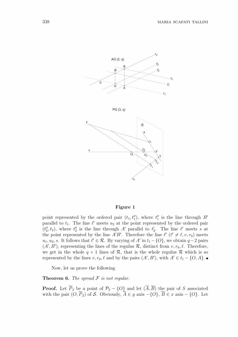
338 maria scafati tallini
AG (2, q)
PG (3, q)
p
A
L
s
Yv
U
T
T
U
T
u
r
l
t
t
t”
t’
t’
t”
1
1
1
2
2
2
o
2
2
2
1
1A’
B
0
B’
Figure 1
point represented by the ordered pair (t1, t′′1), where t′′1 is the line through B′
parallel to t1. The line `′ meets u2 at the point represented by the ordered pair(t′′2, t2), where t′′2 is the line through A′ parallel to t′2. The line `′ meets s atthe point represented by the line A′B′. Therefore the line `′ (`′ 6= `, v, r0) meetsu1, u2, s. It follows that `′ ∈ R. By varying of A′ in t1−O, we obtain q−2 pairs(A′, B′), representing the lines of the regulus R, distinct from v, r0, `. Therefore,we get in the whole q + 1 lines of R, that is the whole regulus R which is sorepresented by the lines v, r0, ` and by the pairs (A′, B′), with A′ ∈ t1−O, A.
Now, let us prove the following
Theorem 6. The spread F is not regular.
Proof. Let P 2 be a point of P2 − O and let (A,B) the pair of S associatedwith the pair (O, P 2) of S. Obviously, A ∈ y axis −O, B ∈ x axis− O. Let

maximal partial line spreads of PG(3, q), q even 339
I be the hyperbolic quadric of PG(3, 22n) containing the lines v, r0 and `(A, B) ofF . Let R be the regulus of I containing such lines. Let `′ be a line of R distinctfrom v, r0 and `(A, B). Since the line `′ does not meet v (since it belongs to thesame regulus of v) and does not belong to the plane π, since it does not meet r0,it belongs to the class a) of [3] and therefore is represented by an ordered pair(A′, B′) of distinct points of AG(2, 22n).
By Theorem 5, we get:
A′ ∈ y axis− O, A,B′ ∈ x axis− O, B,A′B′ is parallel to AB.
We remark that `′ /∈ F ′. For, ` is obviously distinct from v and r0. Moreover,it is easy to prove that `′ 6= `(AB), for any pair (A, B) associated with a pair(P1, P2) of S, with P1 6= O. It is now to prove that `′ is distinct from each of thelines `(AB), with (A,B) associated with (O,P2), P2 ∈ P2 − O. To do this, letT be the point common to the line through A′ parallel to the x axis and to theline through B′ parallel to the y axis. The distinct points O, T2, T are collinearover a line b, as it is easy to prove. If the pair (A′, B′) is associated with a pair(O, P2), P2 ∈ P2−O, necessarily T2 = P2 and therefore T ∈ P2, a contradiction,since the line b cannot meet P2 at three distinct points. The contradiction provesthat (A′, B′) is not associated with any pair (O,P2), P2 ∈ P2 − O and then`′ ∈ F ′. The previous remark is therefore proved. It follows that R is not entirelyconsisting of lines of I and hence it is not regular.
By the above arguments, we get that in PG(3, 22n) there is a total non-regularline spread. As such a spread gives rise to an affine non-desarguesian translationplane of order 24n, we get the following
Theorem 7. For any q = 22n, n an integer, n ≥ 1, there exists a non-desarguesian affine plane of order 24n.
Let T be the following set of lines of PG(3, 22n):
T = `(A,B) : (A,B) is associated with (O,P2), P2 ∈ P2 − O ∪ v, r0.
The set T is a subset of F and has size q+1, but T is not a regulus of PG(3, 22n),since T contains v, r0 and `(A, B) and does not contain `′(A′, B′) (see Theorem 6)which is a line of the regulus R containing v, r0 and `(A,B). Let T1 and T2 bethe points of π − Y represented by the x axis and the y axis, respectively.The line U2T1 of PG(3, 22n) meets v at U2, r0 at T1 and `(A,B) ∈ T − v, r0at the point represented by the ordered pair (tA, x axis), where tA is the line ofAG(2, 22n) through A and parallel to the x axis. It follows that the line U2T1
meets all the lines of T . The line U1T2 of PG(3, 22n) meets v at U1, r0 at T2 and`(A,B) ∈ T − v, r0 at the point represented by the ordered pair (y axis, tB),where tB is the line of AG(2, 22n) through B parallel to the y axis. It follows that

340 maria scafati tallini
U1T2 meets all the lines of T . The line U1T2 of PG(3, 22n) meets v at U1, r0 at T2
and `(A,B) ∈ T −v, r0 at the point represented by the ordered pair (y axis, tB),where tB is the line of AG(2, 22n) through B parallel to the y axis. It follows thatU1T2 meets all the lines of T . The lines U1T2 and U2T1 are mutually skew (as it iseasy to prove by using the representation [3] of U1T2 − U1 and of U2T1 − U2in AG(2, 22n), or equivalently considering that the lines of T are mutually skew).Now let
F = (F − T ) ∪ U1T2, U2T1.Obviously, F is a line spread of PG(3, 22n). Moreover, F is also maximal. For,let ` be a line of PG(3, 22n) not meeting any line of F .
Then the points of ` range over the q + 1 lines of T and it is ` ∩ U1T2 = ∅,`∩U2T1 = ∅. Then the hyperbolic quadric of PG(3, 22n) containing the three linesU1T2, U2T1 and ` admits T as one of its reguli. A contradiction, since T is nota regulus of PG(3, 22n). The contradiction proves that every line of PG(3, 22n)meets some line of F and then F is maximal. Moreover
|F| = q2 − q + 2.
Therefore, the following theorem holds:
Theorem 8. In PG(3, 22n), n integer n ≥ 1, there is a maximal non-total linespread of size q2 − q + 2.
This result was obtained by Freeman [1] in 1980, who constructed an examplewhich was the only before this research. Here, we construct a maximal non-totalline spread for q even of PG(3, 22n), using only the geometry of the affine planeAG(2, 22n). The cardinality q2− q +2 is the maximum known till now, except thesporadic case, for q = 7, found by Heden [2].
References
[1] Freeman, J.W., Reguli and pseudoreguli in PG(3, 22n), Geom. Dedicata,9 (1980), 267-280.
[2] Heden, O., A greedy search for maximal partial spreads in PG(3, 7), ArsComb., 32 (1991), 253-255.
[3] Scafati Tallini, M., Representation of the projective space P (τ, k) in theaffine plane A(2, k), Proc. Conference on Error-Correcting Codes, Crypto-graphy and Finite Geometries, Amer. Math. Soc. (Eds. A. Bruen andD. Wehlan) (2010), 109-122.
Accepted: 28.06.2012
italian journal of pure and applied mathematics – n. 29−2012 (341−350) 341
Hv-STRUCTURES AND THE BAR IN QUESTIONNAIRES
Pipina Nikolaidou
Thomas Vougiouklis
Democritus University of ThraceSchool of Education681 00 AlexandroupolisGreecee-mail: [email protected]
Abstract. The class of hyperstructures called Hv-structures has been studied fromseveral aspects as well as in connection with many other topics of mathematics. Here wepresent applications obtained from social sciences mainly the ones used questionnaires.Moreover we improve the procedure of the filling the questionnaires, using the barinstead of Likert scale, on computers where we write down automatically the results sothey are ready for research.
Key Words and Phrases: hyperstructures, Hv-structures, hopes.
AMS Subject Classification: 20N20, 16Y99.
1. Basic definitions
We deal with the theory of hyperstructures introduced by Marty in 1934 [12].For basic definitions and applications on the related theory one can see the books[3],[4],[7],[16] and related survey papers as the [6]. More specifically we focus on thelarge class of hyperstructures called Hv-structures introduced in 1990 [15], whichsatisfy the weak axioms where the non-empty intersection replaces the equality.Basic definitions on the topic are the following:
In a set H equipped with a hyperoperation (abbreviation hyperoperation= hope) · : H ×H → P (H)− ∅, we abbreviate by
WASS the weak associativity : (xy)z ∩ x(yz) 6= ∅, ∀x, y, z ∈ H and by
COW the weak commutativity : xy ∩ yx 6= ∅, ∀x, y ∈ H
The hyperstructure (H, ·) is called Hv-semigroup if it is WASS, it is calledHv-group if it is reproductive Hv-semigroup, i.e., xH = Hx = H, ∀x ∈ H. Thehyperstructure (R, +, ·) is called Hv-ring if both (+) and (·) are WASS, the re-production axiom is valid of (+) and (·) is weak distributive with respect to (+):
x(y + z) ∩ (xy + xz) 6= ∅, (x + y)z ∩ (xz + yz) 6= ∅, ∀x, y, z ∈ R.

342 pipina nikolaidou, thomas vougiouklis
Motivations. The motivation for Hv-structures is the following [16]: We knowthat the quotient of a group with respect to an invariant subgroup is a group.F. Marty from 1934, states that, the quotient of a group with respect to anysubgroup is a hypergroup. Finally, the quotient of a group with respect to anypartition (or equivalently to any equivalence relation) is an Hv-group.
Specifying this motivation we remark: Let (G, ·) be a group and R be anequivalence relation (or a partition) in G, then (G/R, ·) is an Hv-group, thereforewe have the quotient (G/R, ·)/β* which is a group, the fundamental one. Remarkthat the classes of the fundamental group (G/R, ·)/β* are a union of some of theR-classes. Otherwise, the (G/R, ·)/β* has elements classes of G where they forma partition which classes are larger than the classes of the original partition R.
In an Hv-semigroup the powers of an element h ∈ H are defined as follows:h1 = h, h2 = h · h, ..., hn = h h ... h, where () denotes the n-ary circlehope, i.e. take the union of hyperproducts, n times, with all possible patterns ofparentheses put on them. An Hv-semigroup (H, ·) is called cyclic of period s, ifthere exists an element g, called generator, and a natural number s, the minimumone, such that H = h1∪h2...∪hs. Analogously the cyclicity for the infinite periodis defined [16]. If there is an element h and a natural number s, the minimumone, such that H = hs, then (H, ·) is called single-power cyclic of period s.
The main tool to study hyperstructures are the fundamental relations β*, γ*and ε*, which are defined, in Hv-groups, Hv-rings and Hv-vector spaces, resp., asthe smallest equivalences so that the quotient would be group, ring and vectorspace, resp. The relation β* was introduced by M. Koskas in 1970 [11] and wasmainly studied intensively and in depth by Corsini [3]. The relations γ* and ε*,were introduced by T. Vougiouklis [15],[16],[17] and he named them Fundamental.A way to find the fundamental classes is given by theorems as the following [16]:
Theorem 1.1 Let (H, ·) be an Hv-group and denote by U the set of all finiteproducts of elements of H. We define the relation β in H by setting xβy iffx, y ⊂ u where u ∈ U . Then β* is the transitive closure of β.
An element is called single if its fundamental class is singleton [16].
Fundamental relations are used for general definitions. Thus, an Hv-ring(R, +, ·) is called Hv-field if R/γ* is a field.
Let (H, ·), (H, ∗) be Hv-semigroups defined on the same set H. (·) is calledsmaller than (∗), and (∗) greater than (·), iff there exists an
f ∈ Aut(H, ∗) such that xy ⊂ f(x ∗ y), ∀x, y ∈ H.
Then we write · ≤ ∗ and we say that (H, ∗) contains (H, ·). If (H, ·) is astructure then it is called basic structure and (H, ∗) is called Hb − structure.
Theorem 1.2 (The Little Theorem). Greater hopes than the ones which areWASS or COW, are also WASS or COW, respectively.
Hv-structures and the Bar in questionnaires 343
This Theorem leads to a partial order on Hv-structures and mainly to acorrespondence between hyperstructures and posets. The determination of allHv-groups and Hv-rings is very interesting but hard.
To compare classes we can see the small sets. The problem of enumerationand classification of Hv-structures, or of classes of them, was started very earlybut recently we have interesting results by using computers. The problem iscomplicate in Hv-structures because we have great numbers. The partial orderintroduced in Hv-structures restrict the problem in finding the minimal, up toisomorphisms, Hv-structures. In this direction we have recently results by Bayonand Lygeros as the following [1]:
In a set with two elements, then there are 20 Hv-groups, up to isomorphism.In sets with three elements: There are 6.494 minimal isomorphisms-groups.
The 137 are abelians and 6.357 are not; the 6.152 are cyclic and 342 are not. Thenumber of Hv-groups with three elements is 1.026.462. The 7.926 are abelians,1.018.536 are not; 1.013.598 are cyclic and 12.864 are not. 16 are very thin.
The number of Hv-groups with 4 elements with scalar unit is 631.609.There are 8.028.299.905 abelian Hv-groups, the 7.995.884.377 are cyclic and the32.415.528 are not. There are 10.614.362 abelian hypergroups: the 10.607.666 arecyclic and the 6.696 are not. Notice that there are only 97 canonical hypergroups.
Definition 1.3 [18],[19]. Let (H, ·) be hypergroupoid. We remove h ∈ H, if weconsider the restriction of (·) in the set H − h. h ∈ H absorbs h ∈ H if wereplace h by h and h does not appear in the structure. h ∈ H merges with h ∈ H,if we take as product of any x ∈ H by h, the union of the results of x with bothh, h, and consider h and h as one class with representative h, therefore, h doesnot appear in the hyperstructure.
In 1989 Corsini and Vougiouklis introduced a method to obtain stricter alge-braic structures from given ones through hyperstructure theory. This method wasintroduced before of the Hv-structures, but in fact the Hv-structures appeared inthe procedure.
Definition 1.4 The uniting elements method is the following: Let G be a struc-ture and d be a property, which is not valid, and it is described by a set ofequations. Consider the partition in G for which it is put together, in the sameclass, every pair of elements that causes the non-validity of d. The quotient G/dis an Hv-structure. Then quotient of G/d by the fundamental relation β*, is astricter structure (G/d)β* for which d is valid.
An application of the uniting elements is if more than one property desired.The reason for this is some of the properties lead straighter to the classes: com-mutativity and the reproductivity are easily applicable. One can do this becausethere is a related theorem [16].
The Lie-Santilli isotopies born to solve Hadronic Mechanics problems. San-tilli proposed [13] a ’lifting’ of the trivial unit matrix of a normal theory into anowhere singular, symmetric, real-valued, new matrix. The original theory is re-constructed such as to admit the new matrix as left and right unit. The isofields
344 pipina nikolaidou, thomas vougiouklis
needed correspond to Hv-structures called e-hyperfields which are used in physicsor biology. Definition: Let (Ho, +, ·) be the attached Hv-field of the Hv-semigroup(H, ·). If (H, ·) has a left and right scalar unit e, then (Ho, +, ·) is an e-hyperfield,the attached Hv-field of (H, ·).
Most of Hv-structures are used in Representation (abbreviate by rep) Theory.Reps of Hv-groups can be considered either by generalized permutations or by Hv-matrices [14],[16],[19]. Reps by generalized permutations can be achieved by usingtranslations. In the rep theory the singles are playing a crucial role.
The rep problem by Hv-matrices is the following:Hv-matrix is called a matrix if has entries from an Hv-ring. The hyperproduct
of Hv-matrices A = (aij) and B = (bij), of type m× n and n× r, respectively, isa set of m× r Hv-matrices, defined in a usual manner:
A ·B = (aij) · (bij) = C = (cij)|cij ∈ ⊕∑
aik · bkj,
where (⊕) denotes the n-ary circle hope on the hyperaddition.
Definition 1.5 Let (H, ·) be an Hv-group, (R, +, ·) an Hv-ring, MR=(aij)|aij∈R,then any map
T : H → MR : h → T (h) with T (h1h2) ∩ T (h1)T (h2) 6= ∅,∀h1, h2 ∈ H,
is called Hv-matrix rep. If T (h1h2) ⊂ T (h1)T (h2), then T is an inclusion rep, ifT (h1h2) = T (h1)T (h2), then T is a good rep.
Hopes on any type of matrices can be defined, these are called helix hopes[8], [25].
2. The ∂-hopes
In [20],[21],[22] we defined a hope, in a groupoid with a map f on it called theta ∂.
Definition 2.1 Let (G, ·) be groupoid (resp., hypergroupoid) and f : G → G bea map. We define a hope (∂), on G as follows
x∂y = f(x) ·y, x ·f(y), ∀x, y ∈ G. (resp. x∂y = (f(x) ·y)∪ (x ·f(y)), ∀x, y ∈ G
If (·) is commutative then (∂) is commutative. If (·) is COW then (∂) is COW.Let (G, ·) be groupoid (resp., hypergroupoid) and f : G → P (G)−∅ be any
multivaued map. We define the (∂), on G as follows x∂y = (f(x) · y) ∪ (x · f(y)),∀x, y ∈ G.
Let (G, ·) be groupoid fi : G → G, i ∈ I, be a set of maps on G. Thef∪ : G → P (G) : f∪(x) = fi(x)|i ∈ I, is the union of fi(x). We have the uniontheta-hope (∂), on G if we take f∪(x). If we take f ≡ f ∪ (id), then we have theb-theta-hope.
Motivation for the definition of the theta-hope is the map derivative whereonly the multiplication of functions can be used.

Hv-structures and the Bar in questionnaires 345
Properties 2.2 If (G, ·) is a semigroup, then:
1. For every f, the (∂) is WASS
2. If f is homomorphism and projection , i.e f 2 = f , then (∂) is associative.
3. If (G, ·) is a semigroup then, for every f, the b-theta-hope (∂) is WASS.
4. Reproductivity. If (·) is reproductive then (∂) is also reproductive.
5. Commutativity. If (·) is commutative then (∂) is commutative. If f is intothe centre of G, then (∂) is a commutative. If (·) is a COW then, (∂) is aCOW.
6. Unit elements. u is right unit if x∂u = f(x)·u, x·f(u) 3 x. Sof(u) = e, ife is a unit in (G, ·).The elements of the kernel of f, are the units of (G, ∂). Inhypergroups does not necessarily exist any unit element and if there exists aunit this is not necessarily unique. Moreover the ∂-hopes do not have alwaysthe unit element of the group as unit for the corresponding ∂-hope. This isso because e∂e = f(e)e, ef(e) = f(e)
7. Inverse elements. Let (G, ·) be a monoid with unit e and u be a unit in(G, ∂), then f(u) = e.. For given x, the x′ is an inverse with respect to u,if x∂x′ = f(x) · x′, x · f(x′) 3 u and x′∂x = f(x′) · x, x′ · f(x) 3 u.So, x′ = (f(x))−1u and x′ = u(f(x))−1 are the right and left inverses,respectively.We have two-sided inverses iff f(x)u = uf(x)
Proposition 2.3 Let (G, ·) be, then for all maps f : G → G, the (G, ∂) is anHv-group.
Motivation. For the definition of the theta-hope is the map derivative whereonly the multiplication of functions can be used. Therefore, in these terms, fortwo functions s(x), t(x), we have s∂t = s′t, st′, where (′) denotes the derivative.
Proposition 2.4 Let g ∈ G is a generator of the group (G, ·). Then,
(a) for every f, g is a generator in (G∂), with period at most n.
(b) suppose that there exists an element w such that f(w) = g, then the elementw is a generator in (G, ∂), with period at most n.
There is connection of ∂-hopes with other hyperstructures:
Example. P -hopes [16]. Let (G, ·) be a commutative semigroup and P ⊂ G.Consider the multivalued map f such that f(x) = P · x, ∀x, y ∈ G.
Then we have x∂y = x · y · P, ∀x, y ∈ G.So, the ∂-hope coincides with the well known class of P -hopes [22].One can define ∂-hopes on rings and other more complicate structures, where
more than one ∂-hopes can be defined. Moreover, one can replace structures byhyper ones or by Hv-structures, as well.

346 pipina nikolaidou, thomas vougiouklis
3. The bar in questionnaires
During last decades hyperstructures seem to have a variety of applications not onlyin other branches of mathematics but also in many other sciences including thesocial ones. These applications range from biomathematics and hadronic physicsto automata theory, to mention but a few. This theory is closely related to fuzzytheory; consequently, hyperstructures can now be widely applicable in industryand production, too.
In several papers, such as [2], [5], [13], [24], one can find numerous applica-tions; similarly, in the books [4], [7] a wide variety of applications is also presented.
An important new application, which combines hyperstructure theory andfuzzy theory, is to replace in questionnaires the scale of Likert by the bar ofVougiouklis & Vougiouklis. The suggestion is the following [10]:
Definition 3.1 ”In every question substitute the Likert scale with ’the bar’ whosepoles are defined with ’0’ on the left end, and ’1’ on the right end:
0 1
The subjects/participants are asked instead of deciding and checking a specificgrade on the scale, to cut the bar at any point s/he feels expresses her/his answerto the specific question”.
The use of the bar of Vougiouklis & Vougiouklis instead of a scale of Likerthas several advantages during both the filling-in and the research processing. Thefinal suggested length of the bar, according to the Golden Ratio, is 6.2cm, see[24]. Several advantages on the use of the bar instead of scale one can find in [10].
4. A computerizing filling questionnaires
We present now a program of filling a questionnaire on a computer such that theresults automatically can be transferred for research elaboration.
There are several advantages of the bar one of them is the time of filling thequestionnaire. The only disadvantage of the bar is to transfer the data collectionto a computer for elaboration. At this point, we present an implemented appli-cation to overcome the problems raised during the transferring the data. Thisapplication overcomes the problem of inputting data from questionnaires to pro-cessing and eliminates time of data collection, transferring data directly for anykind of elaboration.
The application has been implemented using Visual Basic and the data isbeing saved on a Microsoft Access Database. The application is based on ”events”and an OleDbConnection is used to connect the program with the database.
Filling-in such questionnaire can be easily achieved by using this application,as it is based on a very simple user interface. The participants have to ”click” onthe bar, in order to indicate the point that satisfies their answer on the questionmade. The user has the opportunity to change his answer by ”clicking” on anotherpoint anytime before submit.
Hv-structures and the Bar in questionnaires 347
The results are being saved on a simple database (Microsoft Access Database)indicating the exact point each participant has ”cut” the bar
5. Applications
One problem in research is to describe mathematical models using theta-hopes.Such a problem is the following [23]:
Problem 5.1 In the research processing suppose that we want to use Likert scaledividing the continuum [01] both by, first, into equal steps (segments) and, second,into equal-area spaces according to Gauss distribution [9], [24]. If we considerboth types of divisions into n segments, then the continuum [01] is divided into2n − 1 segments, if n is odd number and into 2(n − 1) segments, if n is evennumber. We can number the segments and we can consider as an organized devisethe group (Zk,⊕) where k = 2n − 1 or 2(n − 1). Then we can obtain severalhyperstructures using ∂-hopes as the following way: We can have two partitionsof the final segments, into n classes either using the division into equal steps or theGauss distribution by putting in the same class all segments that belong (a) to theequal step or (b) to equal-area spaces according to Gauss distribution. Then wecan consider two kinds of maps (i) a multi-map where every element correspondsto the hole class or (ii) a map where every element corresponds to one special fixedelement of the same class. Using these maps we define the ∂-hopes and we obtainthe corresponding Hv-structure.
An application on this direction is the following construction [23]:
Construction 5.2 Consider a group (G, ·) and suppose take a partition Gi, i ∈ I,of the G. Select and fix an element gi of each partition class Gi, and considerthe map
f : G → G such that f(x) = gi, ∀x ∈ Gi,
then (G, ∂) is an Hv-group. Moreover, the fundamental group (G/R, ·)/β* is(up to isomorphism) a subgroup of the corresponding fundamental group (G, ∂)/β*.
Remark. In the above construction, if one of the selected elements is the unitelement e of the group (G, ·), otherwise, if there exist an element z ∈ G such thatf(z) = e, then we have (G/R, ·)/β*= (G, ∂)/β*.
Proposition 5.3 Suppose (G, ·) be a group and Gi, i ∈ I be a partition of G. Forany class we fix a gi ∈ Gi, and take the map f : G → G : f(x) = gi,∀x ∈ Gi. Iffor the unit element e, in (G, ·), we have f(e) = e, i.e. e is any fixed element, thene is also a unit element of the Hv-group (G, ∂). Moreover (f(x))−1 is an inverseelement in the ∂-Hv-group (G, ∂), of x.
Now, we conclude with an example of the above Construction:

348 pipina nikolaidou, thomas vougiouklis
Example 5.4 Suppose that we take the case of the Likert scale with 5 equalsteps: [0− 1.24− 2.48− 3.72− 4.96− 6.2] and the Gauss 5 equal areas: [0− 2.4−2.9− 3.3− 3.8− 6.2] we have 9 segments as follows
[0− 1.24− 2.4− 2.48− 2.9− 3.3− 3.72− 3.8− 4.96− 6.2]
Therefore, if we consider the set (Z9,+) and if we name the above segments by0, 1, 2, ..., 8 then if we consider the Gauss partition: 0, 1, 2, 3, 4, 5, 6, 7, 8we take, according to the above Construction, the map f such that f(0) = 0,f(1) = 0, f(2) = 2, f(3) = 2, f(4) = 4, f(5) = 5, f(6) = 5, f(7) = 7, f(8) = 7,then we obtain the following table:
∂ 0 1 2 3 4 5 6 7 80 0 0,1 2 2,3 4 5 5,6 7 7,81 0,1 1 2,3 3 4,5 5,6 6 7,8 82 2 2,3 4 4,5 6 7 7,8 0 0,13 2,3 3 4,5 5 6,7 7,8 8 0,1 14 4 4,5 6 6,7 8 0 0,1 2 2,35 5 5,6 7 7,8 0 1 1,2 3 4,36 5,6 6 7,8 8 0,1 1,2 2 3,4 47 7 7,8 0 0,1 2 3 3,4 5 5,68 7,8 8 0,1 1 2,3 4,3 4 5,6 6
Remark that, for the Hv-group (Z9, ∂), the elements 0 and 1 are unit elements.(Z9, ∂) is cyclic where the elements 2, 3, 4, 5, 6, 7 and 8 are generators with period6, 7, 6, 9, 6, 7 and 7 respectively.
References
[1] Bayon, R., Lygeros, N., Advanced results in enumeration of hyperstruc-tures, J. Algebra, 320 (2008) 821-835.
[2] Chvalina, J., Hoskova, S., Modelling of join spaces with proximities byfirst-order linear partial differential operators, no. 21 (2007), 177-190.
[3] Corsini, P., Prolegomena of Hypergroup Theory, Aviani Editore, 1993.
[4] Corsini, P., Leoreanu, V., Application of Hyperstructure Theory, KluwerAcademic Pub., 2003.
[5] Davvaz, B., On Hv-rings and Fuzzy Hv-ideals, J.Fuzzy Math., vol. 6, no.1 (1998), 33-42.
[6] Davvaz, B., A brief survey of the theory of Hv-structures, 8th AHA,Greece, Spanidis (2003), 39-70.
Hv-structures and the Bar in questionnaires 349
[7] Davvaz, B., Leoreanu, V., Hyperring Theory and Applications, Inter-national Academic Press, 2007.
[8] Davvaz, B., Vougioukli, S., Vougiouklis, T., On the multiplicative-rings derived from helix hyperoperations, Utilitas Mathematica, 84 (2011),53-63.
[9] Kambaki-Vougioukli, P., Karakos, A., Lygeros, N., Vougiou-klis, T., Fuzzy instead of discrete, Annals of Fuzzy Mathematics and In-formatics, vol. 2, no. 1 (2011), 81-89.
[10] Kambaki-Vougioukli, P., Vougiouklis, T., Bar instead of scale, RatioSociologica, 3, (2008), 49-56.
[11] Koskas, M., Groupoides, demi-groupoides et hypergroups, J. Math. PuresAppl., 49 (9), (1970), 155-192.
[12] Marty, F., Sur un generalisation de la notion de groupe, 8eme CongresMath. Scandinaves, Stockholm, (1934), 45-49.
[13] Santilli, R.M., Vougiouklis, T., Isotopies, Genotopies, Hyperstruc-tures and Their Applications, New frontiers in Hyperstructures, Hadronic(1996), 1-48.
[14] Vougiouklis, T., Representations of hypergroups by hypermatrices, Ri-vista Mat. Pura ed Appl., no. 2 (1987), 7-19.
[15] Vougiouklis, T., The fundamental relation in hyperrings. The generalhyperfield, 4thAHA, Xanthi 1990, World Scientific (1991), 203-211.
[16] Vougiouklis, T., Hyperstructures and their Representations, Monographsin Mathematics, Hadronic, 1994.
[17] Vougiouklis, T., Some remarks on hyperstructures, Contemporary Ma-thematics, Amer. Math. Society, 184 (1995), 427-431.
[18] Vougiouklis, T., Consructions of Hv-structures with desired fundamentalstructures, New frontiers in Hyperstructues, Hadronic (1996), 177-188.
[19] Vougiouklis, T., On Hv-rings and Hv-representations, Discrete Mathe-matics, Elsevier, 208/209 (1999), 615-620.
[20] Vougiouklis, T., A hyperoperation defined on a groupoid equipped with amap, Ratio Mathematica, 1 (2005), 25-36.
[21] Vougiouklis, T., ∂-operations and Hv-fields, Acta Mathematica Sinica,English S., vol. 23, 6 (2008), 965-972.
[22] Vougiouklis, T., The relation of the theta-hyperoperation (∂) with theother classes of hyperstructures, J. Basic Sciences 4, no. 1 (2008), 135-145.
350 pipina nikolaidou, thomas vougiouklis
[23] Vougiouklis, T., Bar and Theta Hyperoperations, Ratio Mathematica, 21(2011), 27-42.
[24] Vougiouklis, T., Kambaki-Vougioukli, P., On the use of the bar,China-USA Business Review, vol. 10, no. 6 (2011), 484-489.
[25] Vougiouklis, T., Vougiouklis, S., The helix hyperoperations, Italian J.Pure Applied Math., no. 18 (2005), 197-206.
Accepted: 02.07.2012
italian journal of pure and applied mathematics – n. 29−2012 (351−364) 351
RELATED FIXED POINT THEOREM FOR SIX MAPPINGSON THREE MODIFIED INTUITIONISTIC FUZZY METRIC SPACES
Sushil Sharma
Department of MathematicsMadhav Science CollegeVikram UniversityUjjain-456010Indiae-mail: [email protected]
Prashant Tilwankar
Department of MathematicsShri Vaishnav Institute of ManagementIndore-452009Indiae-mail:prashant [email protected]
Abstract. Related fixed point theorems on two or three metric spaces have been provedin different ways. Sharma, Deshpande and Thakur were the first who have establishedrelated fixed point theorem for four mappings on two complete fuzzy metric spaces.Their work was maiden in this line. In this paper we obtain a related fixed pointtheorem for six mappings on three complete modified intuitionistic fuzzy metric spaces.Of course this is a new result on this line.
AMS Subject Classification (2000): 47H10, 54H25.
Keywords: modified intuitionistic fuzzy metric space, common fixed point, Cauchysequence.
1. Introduction
Motivated by the potential applicability of fuzzy topology to quantum particlephysics particularly in connection with both string and e(∞) theory developed byEl Naschie [10], [11], Park introduced and discussed in [24] a notion of intuitionisticfuzzy metric spaces which is based on the idea of intuitionistic fuzzy sets dueto Atanassov [3] and the concept of fuzzy metric space given by George andVeeramani [18]. Actually, Park’s notion is useful in modelling some phenomenawhere it is necessary to study the relationship between two probability functions.It has direct physics motivation in the context of the two-slit experiment as thefoundation of E-infinity of high energy physics, recently studied by El Naschie[12], [13].
352 sushil sharma, prashant tilwankar
Alaca et al. [2] using the idea of intuitionistic fuzzy sets, they defined thenotion of intuitionistic fuzzy metric space as Park [24] with the help of continuoust-norms and continuous t-conorms as a generalization of fuzzy metric space dueto Kramosil and Michalek [22]. Further, they introduced the notion of Cauchysequences in intuitionistic fuzzy metric spaces and proved the well known fixedpoint theorems of Banach [4] and Edelstein [9] extended to intuitionistic fuzzymetric spaces with the help of Grabiec [13]. Turkoglu et al. [30] introducedthe concept of compatible maps and compatible maps of types (α) and (β) inintuitionistic fuzzy metric spaces and gave some relations between the conceptsof compatible maps and compatible maps of types (α) and (β).
Since the intuitionistic fuzzy metric space has extra conditions, Saadati,Sedghi and Shobe [28] modified the idea of intuitionistic fuzzy metric spaces andgave the new notion of intuitionistic fuzzy metric spaces with the help of thenotion of continuous t-representable.
Related fixed point theorems on two or three metric spaces were proved byFisher[14],[15], Nung[23], Popa [24], Jain, Sahu and Fisher [19], Jain, Shrivastavaand Fisher [20], Cho, Kang and Kim [5], Fisher and Murthy [16] and many others.Sharma, Deshpande and Thakur [29] established a related fixed point theorem forfour mappings on two complete fuzzy metric spaces. Deshpande and Pathak [8]intuitionistically fuzzified the results of Sharma, Deshpande and Thakur [29] andproved a related fixed point theorem for two pairs of mappings on two intuitionisticfuzzy metric spaces. In this paper, we extend the results of Deshpande and Pathak[8] and prove a related fixed point theorem for six mappings on three completemodified intuitionistic fuzzy metric spaces.
2. Preliminaries
Definition 2.1. ([26]) A binary operation ∗ : [0, 1] × [0, 1] → [0, 1] is continuoust-norm if ∗ is satisfying the following conditions:
(i) ∗ is commutative and associative,
(ii) ∗ is continuous,
(iii) a ∗ 1 = a for all a ∈ [0, 1],
(iv) a ∗ b ≤ c ∗ d whenever a ≤ c and b ≤ d, a, b, c, d ∈ [0, 1].
Definition 2.2. ([26]) A binary operation ¦ : [0, 1] × [0, 1] → [0, 1] is continuoust-conorm if ¦ is satisfying the following conditions:
(i) ¦ is commutative and associative,
(ii) ¦ is continuous,
(iii) a ¦ 0 = a for all a ∈ [0, 1],
(iv) a ¦ b = c ¦ d whenever a ≤ c and b ≤ d, a, b, c, d ∈ [0, 1].
related fixed point theorem for six mappings ... 353
Lemma 2.1. ([7]) Consider the set L∗ and operation ≤L∗ defined by
L∗ = (x1, x2) : (x1, x2) ∈ [0, 1]2 and x1 + x2 ≤ 1(x1, x2) ≤L∗ (y1, y2) ⇔ x1 ≤ y1 and x2 ≥ y2, for every (x1, x2), (y1, y2) ∈ L∗.
Then (L∗, ≤L∗) is a complete lattice.
Definition 2.3. ([3]) An intuitionistic fuzzy set Aζ,η in a universe U is an ob-ject Aζ,η = (ζA(u), ηA(u))| u ∈ U, where, for all u ∈ U, ζA(u) ∈ [0, 1] andηA(u) ∈ [0, 1] are called the membership degree and the non-membership degree,respectively, of u in Aζ,η, and, furthermore, they satisfy ζA(u) + ηA(u) ≤ 1.
For every zi = (xi, yi) ∈ L∗, if ci ∈ [0, 1] such thatn∑
j=1
cj = 1, then it is
easy that
(2.1) c1(x1, y1) + · · ·+ cn(xn, yn) =n∑
j=1
cj (xj, yj) =
(n∑
j=1
cjxj,
n∑j=1
cjyj
)∈ L∗.
We denote its units by 0L∗ = (0, 1) and 1L∗ = (1, 0). Classically, a triangularnorm ∗ = T on [0, 1] is defined as an increasing, commutative, associative map-ping T : [0, 1]2 → [0, 1] satisfying T (1, x) = 1∗x = x, for all x ∈ [0, 1]. A triangu-lar conorm S = ¦ is defined as an increasing, commutative, associative mappingS : [0, 1]2 → [0, 1] satisfying S(0, x) = 0 ¦ x = x, for all x ∈ [0, 1]. Using thelattice (L∗, ≤L∗) these definitions can be straightforwardly extended.
Definition 2.4. ([6]) A triangular norm (t-norm) on L∗ is a mapping τ : (L∗)2 → L∗
satisfying the following conditions:
(∀ x ∈ L∗)(τ(x, 1L∗) = x) (boundary condition),
(∀(x, y) ∈ (L∗)2)(τ(x, y) = τ(y, x)) (commutativity),
(∀(x, y, z) ∈ (L∗)3)(τ(x, τ(y, z)) = τ(τ(x, y), z)) (associativity),
(∀(x, x′, y, y′) ∈ (L∗)4)(x ≤L∗ x′) and (y ≤L∗ y′ → τ(x, y) ≤L∗ τ(x′, y′))(monotonicity).
Definition 2.5. ([6], [7]) A continuous t-norm τ on L∗ is called continuous t-representable if and only if there exist a continuous t-norm ∗ and a continuoust-conorm ¦ on [0, 1] such that, for all x = (x1, x2), y = (y1, y2) ∈ L∗,
τ(x, y) = (x1 ∗ y1, x2 ¦ y2).
Now, define a sequence τn recursively by τ 1 = τ and
τn(x(1), ..., x(n+1)) = τ(τn−1(x(1), ..., x(n), x(n+1)) for n ≥ 2 and x(i) ∈ L∗.
Definition 2.6. ([28]) Let M,N are fuzzy sets from X2 × (0, +∞) to [0, 1]such that M(x, y, t) + N(x, y, t) ≤ 1 for all x, y ∈ X and t > 0. The 3-tuple(X,MM,N , τ) is said to be an intuitionistic fuzzy metric space if X is an arbi-trary (non-empty) set, τ is a continuous t-representable and MM,N is a mappingX2 × (0, +∞) → L∗ (an intuitionistic fuzzy set, see Definition 2.3) satisfying thefollowing conditions for every x, y ∈ X and t, s > 0:
354 sushil sharma, prashant tilwankar
(a) MM,N(x, y, t)>L∗0L∗ ;
(b) MM,N(x, y, t) = 1L∗ if and only if x = y;
(c) MM,N(x, y, t) = MM,N(y, x, t);
(d) MM,N(x, y, t + s) ≥L∗ τ(MM,N(x, z, t),MM,N(z, y, s));
(e) MM,N(x, y, ·) : (0,∞) → L∗ is continuous.
In this case, MM,N is called an intuitionistic fuzzy metric.Here,
MM,N(x, y, t) = (M(x, y, t), N(x, y, t)).
Example 2.1. ([28]) Let (X, d) be a metric space. Denote
τ(a, b) = (a1b1, min(a2 + b2, 1))
for all a = (a1, a2) and b = (b1, b2) ∈ L∗ and let M and N be fuzzy sets onX2 × (0,∞) defined as follows:
MM, N(x, y, t)=(M(x, y, t), N(x, y, t))=
(htn
htn + md(x, y),
md(x, y)
htn + md(x, y)
)
for all t, h, m, n ∈ R+.
Then, (X,MM,N ,τ) is an intuitionistic fuzzy metric space.
Example 2.2. ([28]) Let X = N . Define
τ(a, b) = (max(0, a1 + b1 − 1), a2 + b2 − a2b2)
for all a = (a1, a2) and b = (b1, b2) ∈ L∗ and let M and N be fuzzy sets onX2 × (0,∞) defined as follows:
MM,N(x, y, t) = (M(x, y, t), N(x, y, t)) =
(x
y,
y − x
y
)if x ≤ y,
(y
x,
x− y
x
)if y ≤ x,
for all x, y ∈ X and t > 0. Then (X,MM, N ,τ) is an intuitionistic fuzzy metricspace.
Definition 2.7. ([28]) A sequence xn in an intuitionistic fuzzy metric space(X,MM, N , τ) is called a Cauchy sequence if for each 0 < ε < 1 and t > 0, thereexists n0 ∈ N such that
MM,N(xn, ym, t) >L∗(Ns(ε), ε)

related fixed point theorem for six mappings ... 355
and for each n,m ≥ n0, here Ns is the standard negator. The sequence xn is saidto be convergent to x ∈ X in the intuitionistic fuzzy metric space (X,MM,N , τ)
and denoted by xn
MM,N−→ x if MM,N(xn, x, t) → 1L∗ whenever n → ∞ for everyt > 0. An intuitionistic fuzzy metric space is said to be complete if and only ifevery Cauchy sequence is convergent.
Lemma 2.2. ([27]) Let MM, N be an intuitionistic fuzzy metric space. Then, forany t > 0, MM,N(x, y, t) is non-decreasing with respect to t, in (L∗,≤L∗), for allx, y in X.
Lemma 2.3. ([1]) Let (X,MM,N , τ) be a modified intuitionistic fuzzy metricspace. For each λ ∈ (0, 1), define the map Eλ : X2 → R+ ∪ 0 by
Eλ(x, y) = inft > 0 : MM,N(x, y, t)>L∗(1− λ, λ),
then
(a) For each λ ∈ (0, 1), we have a µ ∈ (0, 1) such that
Eλ(x1, xn) ≤ Eµ(x1, x2) + Eµ(x2, x3) + · · ·+ Eµ(xn−1, xn),
for any x1, x2, x3, ..., xn ∈ X.
(b) The sequence xnn∈N in X is convergent to x if and only if Eλ(xn, x) → 0.
Also, the sequence xnn∈N is a Cauchy sequence in X if and only if it is aCauchy sequence with respect to Eλ.
Lemma 2.4. ([21]) Let (X,MM, N ,τ) be an intuitionistic fuzzy metric space. Iffor a sequence xn in X, there exists k ∈ (0, 1) such that
MM,N(xn, xn+1, kt) ≥L∗ MM,N(xn−1, xn, t), for all n and for all t,
then xn is a Cauchy sequence in X.
Proof. Let (X,MM, N ,τ) be an intuitionistic fuzzy metric space. Let for asequence xn in X, there exists k ∈ (0, 1) such that
MM, N(xn, xn+1, kt) ≥L∗ MM, N(xn−1, xn, t), for all n and t,
then
MM,N(xn, xn+1, t) ≥L∗ MM,N
(xn−1, xn,
t
k
)≥L∗ MM,N
(xn−2, xn−1,
t
k2
)
. . . ≥L∗ MM,N(x0, x1,t
kn), for all n.
356 sushil sharma, prashant tilwankar
Now
Eλ(xn+1, xn) = inft > 0 : MM,N(xn+1, xn, t) ≥L∗ (1− λ, λ)
≤ inft > 0 : MM,N
(x1, x0,
t
kn
)≥L∗ (1− λ, λ)
= infknt > 0 : MM,N(x1, x0, t) ≥L∗ (1− λ, λ)= kn inft > 0 : MM,N(x1, x0, t) ≥L∗ (1− λ, λ)= kn Eλ(x0, x1).
Eλ(xn+1, xn) ≤ knEλ(x0, x1) . . . (A)
Again from Lemma 2.3, for λ ∈ (0, 1), there exists µ ∈ (0, 1) such that
Eλ(xn, xn+p) ≤ Eµ(xn, xn+1) + Eµ(xn+1, xn+2) + · · ·+ Eµ(xn+p−1, xn+p)
≤ kn Eµ(x0, x1) + kn+1 Eµ(x0, x1) + · · ·+ kn+p−1 Eµ(x0, x1),
using (A)
= (kn + kn+1 + · · ·+ kn+p−1)Eµ(x0, x1),
=kn
1− kEµ(x0, x1), as 0 < k < 1,
which tends to 0, as n → ∞. Hence xn is a Cauchy sequence in X.
Lemma 2.5. ([21]) In an intuitionistic fuzzy metric space (X,MM, N ,τ), iffor some x, y in X there exists k ∈ (0, 1) such that
MM, N(x, y, kt) ≥L∗ MM, N(x, y, t), for all t,
then x = y.
Proof. Let for λ ∈ (0, 1)
Eλ(x, y) = inft > 0 : MM,N(x, y, t) ≥L∗ (1− λ, λ)≤ inft > 0 : MM,N(x, y, t/k) ≥L∗ (1− λ, λ)= infkt > 0 : MM,N(x, y, t) ≥L∗ (1− λ, λ)= k inft > 0 : MM,N(x, y, t) ≥L∗ (1− λ, λ)= k Eλ(x, y).
Therefore, Eλ(x, y) = 0. Hence x = y.
Sharma, Deshpande and Thakur [29] established the following related fixedpoint theorem for four mappings on two complete fuzzy metric spaces.
Theorem A. Let (X, M1, ∗) and (Y,M2, ∗) be two complete fuzzy metric spaces.Let A,B be mappings from X into Y and S, T be mappings from Y into X satis-fying the inequalities:
related fixed point theorem for six mappings ... 357
(i) M1(SAx, TBx′, kt) ≥ M1(x, x′, t) ∗M1(x, SAx, t) ∗M1(x′, TBx′, t)
∗M1(SAx, TBx′, t)
(ii) M2(BSy,ATy′, kt) ≥ M2(y, y′, t) ∗M2(y,BSy, t) ∗M2(y′, ATy′, t)
∗ M2(BSy,ATy′, kt)
for all x, x′ in X and y, y′ in Y . If one of the mappings A,B, S, T is continuous,then SA and TB have a unique common fixed point z in X and BS and AT havea unique common fixed point w in Y . Further, Az = Bz = w and Sw = Tw = z.
Deshpande and Pathak [8] intuitionistically fuzzify the results of Sharma,Deshpande and Thakur [29] and proved the following:
Theorem B. (X, M1, N1, ∗, ¦) and (Y, M2, N2, ∗, ¦) be two complete intuitionisticfuzzy metric spaces. Let A,B be mappings from X into Y and let S, T be mappingsfrom Y into X satisfying the inequalities:
(i) M1(SAx, TBx′, kt) ≥ M1(x, x′, t) ∗M1(x, SAx, t) ∗M1(x′, TBx′, t)∗M1(SAx, TBx′, t)
and
N1(SAx, TBx′, kt) ≤ N1(x, x′, t) ¦N1(x, SAx, t) ¦N1(x′, TBx′, t)¦N1(SAx, TBx′, t)
(ii) M2(BSy,ATy′, kt) ≥ M2(y, y′, t) ∗M2(y, BSy, t) ∗M2(y′, ATy′, t)∗M2(BSy, ATy′, t)
and
N2(BSy,ATy′, kt) ≤ N2(y, y′, t) ¦N2(y, BSy, t) ¦N2(y′, ATy′, t)¦ N2(BSy, ATy′, t)
for all x, x′ in X and y, y′ in Y . If one of the mappings A,B, S, T is continuous,then SA and TB have a unique common fixed point z in X and BS and AT havea unique common fixed point w in Y . Further, Az = Bz = w and Sw = Tw = z.
We extend the results of Deshpande and Pathak [8] and prove a related fixedpoint theorem for six mappings on three complete modified intuitionistic fuzzymetric spaces.
3. Main result
Theorem 3.1. Let (X,MM1, N1 ,τ), (Y,MM2, N2 ,τ) and (Z,MM3, N3 ,τ) be threecomplete intuitionistic fuzzy metric spaces. Let A,B be continuous mappings fromX into Y , let S, T be continuous mappings from Y into Z and let P,Q be conti-nuous mappings from Z into X satisfying the inequalities:
358 sushil sharma, prashant tilwankar
(3.1) MM1,N1(PSAx,QTBx′, kt) ≥L∗ MM1, N1(x, x′, t) ∗MM1,N1(x, PSAx, t)
∗MM1,N1(x′, QTBx′, t) ∗MM1,N1(PSAx,QTBx′, t)
(3.2) MM2,N2(APSy,BQTy′, kt) ≥L∗ MM2,N2(y, y′, t) ∗MM2,N2(y,APSy, t)
∗MM2,N2(y′, BQTy′, t) ∗MM2,N2(APSy,BQTy′, t)
(3.3) MM3,N3(SAPz, TBQz′, kt) ≥L∗ MM3,N3(z, z′, t) ∗MM3,N3(z, SAPz, t)
∗MM3,N3(z′, TBQz′, t) ∗MM3,N3(SAPz, TBQz′, t)
for all x, x′ in X, y, y′ in Y and z, z′ in Z, t > 0 and k ∈ (0, 1), then PSA andQTB have a unique common fixed point u in X, APS and BQT have a uniquecommon fixed point v in Y and SAP and TBQ have a unique common fixed pointw in Z. Further, Au = Bu = v, Sv = Tv = w and Pw = Qw = u.
Proof. Let x = x0 be an arbitrary point in X and define sequences xn, ynand zn in X, Y and Z respectively as follows:
Choose a point z1 = Sy1, a point y1 = Ax0, a point x1 = Pz1, a point z2 =Ty2, a point y2 = Bx1 and a point x2 = Qz2. In general, having chosen x2n−2 inX, choose a point y2n−1 = Ax2n−2, a point y2n = Bx2n−1, a point z2n−1 = Sy2n−1,a point z2n = Ty2n, a point x2n−1 = Pz2n−1 and a point x2n = Qz2n for alln = 1, 2, ...
Applying inequality (3.1), we have
(3.4)
MM1,N1(x2n+1, x2n, kt) = MM1,N1(PSAx2n, QTBx2n−1, kt)
≥L∗ MM1,N1(x2n, x2n−1, t) ∗MM1,N1(x2n, PSAx2n, t)
∗MM1, N1(x2n−1, QTBx2n−1, t) ∗MM1,N1(PSAx2n, QTBx2n−1, t)
= MM1,N1(x2n, x2n−1, t) ∗MM1,N1(x2n, x2n+1, t)
∗MM1,N1(x2n−1, x2n, t) ∗MM1,N1(x2n+1, x2n, t)
≥L∗ MM1,N1(x2n, x2n−1, t) ∗MM1,N1(x2n, x2n+1, t)
Similarly, we have
(3.5)MM1,N1(x2n+2, x2n+1, kt) ≥L∗ MM1,N1(x2n+1, x2n, t)
∗MM1,N1(x2n+1, x2n+2, t).
Thus, from (3.4) and (3.5), it follows that
MM1,N1(xn+1, xn+2, kt) ≥L∗ MM1,N1(xn, xn+1, t) ∗MM1,N1(xn+1, xn+2, t),
for n = 1, 2, ....Consequently, for positive integers n, p we have
MM1,N1(xn+1, xn+2, kt) ≥L∗ MM1,N1(xn, xn+1, t) ∗MM1,N1(xn+1, xn+2, t/kp).
Thus, since MM1, N1(xn+1, xn+2, kt) → 1L∗ as p →∞, we have
(3.6) MM1,N1(xn+1, xn+2, kt) ≥L∗ MM1,N1(xn, xn+1, t)
related fixed point theorem for six mappings ... 359
Similarly, applying inequality (3.2) and (3.3), we have
(3.7) MM2,N2(yn+1, yn+2, kt) ≥L∗ MM2,N2(yn, yn+1, t)
(3.8) MM3,N3(zn+1, zn+2, kt) ≥L∗ MM3,N3(zn, zn+1, t)
By Lemma 2.4, xn is a Cauchy sequence in a complete intuitionistic fuzzymetric space X and so has a limit u in X. It follows similarly that the sequencesyn and zn are also Cauchy sequences in complete intuitionistic fuzzy metricspace Y and Z and so have limits v in Y and w in Z.
Using (3.1), we have
MM1,N1(PSAx2n, u, kt) ≥L∗ MM1,N1(PSAx2n, x2n, kt2) ∗MM1,N1(x2n, u, kt
2)
= MM1,N1(PSAx2n, QTBx2n−1,kt2) ∗MM1,N1(x2n, u, kt
2)
≥L∗ MM1,N1(x2n, x2n−1,t2) ∗MM1,N1(x2n, PSAx2n, t
2)
∗MM1,N1(x2n−1, QTBx2n−1,t2)
∗MM1,N1(PSAx2n, QTBx2n−1,t2) ∗MM1,N1(x2n, u, kt
2)
≥L∗ MM1,N1(x2n, x2n−1,t2) ∗MM1,N1(x2n, x2n+1,
t2)
∗MM1,N1(x2n−1, x2n,t2) ∗MM1,N1(x2n+1, x2n, t
2) ∗MM1,N1(x2n, u, kt
2)
Taking limit n →∞, we have
limn→∞
MM1, N1(PSAx2n, u, kt) → 1L∗ .
Thus, we have
(3.9) limn→∞
PSAx2n = u = limn→∞
PSy2n+1
Similarly, we can prove that
(3.10) limn→∞
QTBx2n−1 = u = limn→∞
QTy2n
(3.11) limn→∞
APSy2n−1 = v = limn→∞
APz2n−1
(3.12) limn→∞
BQTy2n = v = limn→∞
BQz2n
(3.13) limn→∞
SAPz2n = w = limn→∞
SAx2n
(3.14) limn→∞
TBQz2n−1 = w = limn→∞
TBx2n−1
Since A and B are continuous, we have
(3.15) limn→∞
Ax2n = Au = v, limn→∞
Bx2n−1 = Bu = v.

360 sushil sharma, prashant tilwankar
Using inequality (3.1), we have
MM1,N1(PSAu, QTBx2n−1, kt) ≥L∗ MM1,N1(u, x2n−1, t) ∗MM1,N1(u, PSAu, t)
∗MM1,N1(x2n−1, QTBx2n−1, t) ∗MM1,N1(PSAu, QTBx2n−1, t).
Letting n →∞ and using (3.10), we have
MM1, N1(PSAu, u, kt) ≥L∗ MM1, N1(u, PSAu, t).
Therefore, by Lemma 2.5 and using (3.15), we have PSAu = u = PSv.Using inequality (3.1), we have
MM1,N1(PSAx2n, QTBu, kt) ≥L∗ MM1,N1(x2n, u, t) ∗MM1,N1(x2n, PSAx2n, t)
∗MM1,N1(u,QTBu, t) ∗MM1,N1(PSAx2n, QTBu, t).
Letting n → ∞ and using (3.9), we have
MM1,N1(u, QTBu, kt) ≥L∗ MM1,N1(u,QTBu, t).
Therefore, by Lemma 2.5 and using (3.15), we have QTBu = u = QTv.Since S and T are continuous, we have
(3.16) limn→∞
Sy2n−1 = Sv = w, limn→∞
Ty2n = Tv = w.
Using inequality (3.2), we have
MM2, N2(APSv, BQTy2n, kt) ≥L∗ MM2, N2(v, y2n, t) ∗MM2, N2(v,APSv, t)
∗MM2, N2(y2n, BQTy2n, t) ∗MM2, N2(APSv,BQTy2n, t).
Letting n →∞ and using (3.12), we have
MM2, N2(APSv, v, kt) ≥L∗ MM2, N2(v,APSv, t).
Therefore, by Lemma 2.5 and using (3.16), we have APSv = v = APw.Using inequality (3.2), we have
MM2,N2(APSy2n−1, BQTv, kt)
≥L∗ MM2,N2(y2n−1, v, t) ∗MM2,N2(y2n−1, APSy2n−1, t)
∗MM2,N2(v,BQTv, t) ∗MM2,N2(APSy2n−1, BQTv, t).
Letting n →∞ and using (3.11), we have
MM2, N2(v,BQTv, kt) ≥L∗ MM2, N2(v,BQTv, t).
Therefore, by Lemma 2.5 and using (3.16), we have BQTv = v = BQw.Since P and S are continuous, we have
(3.17) limn→∞
Pz2n = Pw = u, limn→∞
Qz2n−1 = Qw = u.
related fixed point theorem for six mappings ... 361
Using inequality (3.3), we have
MM3,N3(SAPw, TBQz2n−1, kt) ≥L∗ MM3,N3(w, z2n−1, t) ∗MM3,N3(w, SAPw, t)
∗MM3,N3(z2n−1, TBQz2n−1, t) ∗MM3,N3(SAPw, TBQz2n−1, t).
Letting n → ∞ and using (3.14), we have
MM3, N3(SAPw, w, kt) ≥L∗ MM3, N3(w, SAPw, t).
Therefore, by Lemma 2.5 and using (3.17), we have SAPw = w = SAu.Using inequality (3.3), we have
MM3, N3(SAPz2n, TBQw, kt) ≥L∗ MM3, N3(z2n, w, t) ∗MM3, N3(z2n, SAPz2n, t)
∗ MM3, N3(w, TBQw, t) ∗MM3, N3(SAPz2n, TBQw, t).
Letting n → ∞ and using (3.13), we have
MM3, N3(w, TBQw, kt) ≥L∗ MM3, N3(w, TBQw, t).
Therefore, by Lemma 2.5 and using (3.17), we have TBQw = w = TBu.Thus, we have
(3.18)
PSAu = QTBu = PSv = QTv = Pw = Qw = u,APSv = BQTv = APw = BQw = Au = Bu = v,SAPw = TBQw = SAu = TBu = Sv = Tv = w.
To prove the uniqueness of the fixed point, suppose that PSA and QTB havea common fixed point u′ also.
Using inequality (3.1), we have
MM1,N1(PSAu, QTBu′, kt) ≥L∗ MM1,N1(u, u′, t) ∗MM1,N1(u, PSAu, t)
∗MM1,N1(u′, QTBu′, t) ∗MM1,N1(PSAu, QTBu′, t).
Therefore, we have
MM1, N1(u, u′, kt) ≥L∗ MM1, N1(u, u′, t).
By Lemma 2.5, we have u = u′. Similarly we can prove that v and w are uniquecommon fixed point of APS and BQT and of SAP and TBQ. This completesthe proof.
If we put M1 = M2 = M3 = M and N1 = N2 = N3 = N in Theorem 3.1, weget the following:
Corollary 1. Let (X,MM, N ,τ), (Y,MM, N ,τ) and (Z,MM, N ,τ) be three com-plete intuitionistic fuzzy metric spaces. Let A,B be continuous mappings from Xinto Y , let S, T be continuous mappings from Y into Z and let P,Q be continuousmappings from Z into X satisfying the inequalities:
362 sushil sharma, prashant tilwankar
(3.1) MM,N(PSAx, QTBx′, kt) ≥L∗ MM,N(x, x′, t) ∗MM,N(x, PSAx, t)
∗MM,N(x′, QTBx′, t) ∗MM,N(PSAx, QTBx′, t)
(3.2) MM,N(APSy, BQTy′, kt) ≥L∗ MM,N(y, y′, t) ∗MM,N(y, APSy, t)
∗MM,N(y′, BQTy′, t) ∗MM,N(APSy, BQTy′, t)
(3.3) MM,N(SAPz, TBQz′, kt) ≥L∗ MM, N(z, z′, t) ∗MM, N(z, SAPz, t)
∗MM, N(z′, TBQz′, t) ∗MM, N(SAPz, TBQz′, t)
for all x, x′ in X, y, y′ in Y and z, z′ in Z, t > 0 and k ∈ (0, 1), then PSA andQTB have a unique common fixed point u in X, APS and BQT have a uniquecommon fixed point v in Y and SAP and TBQ have a unique common fixed pointw in Z. Further, Au = Bu = v, Sv = Tv = w and Pw = Qw = u.
If we put A = B, S = T and P = Q in Theorem 3.1, we get the following:
Corollary 2. Let (X,MM1,N1 , τ), (Y,MM2,N2 , τ) and (Z,MM3,N3 , τ) be threecomplete intuitionistic fuzzy metric spaces. Let A be continuous mapping fromX into Y , let S be continuous mapping from Y into Z and let P be continuousmapping from Z into X satisfying the inequalities:
(3.4) MM1,N1(PSAx, PSAx′, kt) ≥L∗ MM1,N1(x, x′, t) ∗MM1,N1(x, PSAx, t)
∗MM1,N1(x′, PSAx′, t) ∗MM1,N1(PSAx, PSAx′, t)
(3.5) MM2,N2(APSy,APSy′, kt) ≥L∗ MM2,N2(y, y′, t) ∗MM2,N2(y,APSy, t)
∗MM2,N2(y′, APSy′, t) ∗MM2,N2(APSy, APSy′, t)
(3.6) MM3,N3(SAPz, SAPz′, kt) ≥L∗ MM3,N3(z, z′, t) ∗MM3,N3(z, SAPz, t)
∗MM3,N3(z′, SAPz′, t) ∗MM3,N3(SAPz, SAPz′, t)
for all x, x′ in X, y, y′ in Y and z, z′ in Z, t > 0 and k ∈ (0, 1), then PSA has aunique common fixed point u in X, APS has a unique common fixed point v inY and SAP has a unique common fixed point w in Z. Further, Au = v, Sv = wand Pw = u.
Remark 3.1. From Theorem 3.1, with P = Q = Ix (the identity mapping on X),we obtain modified intuitionistic version of the results of Sharma, Deshpande andThakur [29] and Deshpande and Pathak [8].
References
[1] Abidi, H., Cho, Y.J., Regan, D.O. and Saadati, R., Common fixedpoint in L-fuzzy metric spaces, Applied Mathematics and Computation, 182(2006), 820-828.
related fixed point theorem for six mappings ... 363
[2] Alaca, C., Turkoglu, D. and Yildiz, C., Fixed points in intuitionisticfuzzy metric spaces, Chaos, Solitons & Fractals, 29 (2006), 1073-1078.
[3] Atanassov, K., Intuitionistic fuzzy sets, Fuzzy Sets and Systems, 20(1986),87-96.
[4] Banach, S., Theoriles Operations Linearies Manograie Mathematyezne,Warsaw, Poland, 1932.
[5] Cho, Y. J., Kang, S.M. and Kim, S.S., Fixed points in two metric spaces,Novi Sad J. Math., 29 (1) (1999), 47-53.
[6] Deschrilver, G., Cornelis, C. and Kerre, E.E., On representationof Intuitionistic fuzzy t-norms and t-conorms, IEEE Trans Fuzzy Sets andSystems, 12 (2001), 45-61.
[7] Deschrilver, G. and Kerre, E.E., On the relationship between someextensions of fuzzy set theory, Fuzzy Sets and Systems, 133 (2003), 517-529.
[8] Deshpande, B. and Pathak, R., Related fixed point theorem on two in-tuitionistic fuzzy metric spaces, J. Korean Soc. Math. Educ. Ser. B.: PureAppl. Math., 16 (4) (2009), 345-357.
[9] Edelstein, M., On fixed and periodic points under contractive mappings,J. London Math. Soc., 37 (1962), 74-79.
[10] El Naschie, On the uncertainty of Cantorian geometry and two-slit expe-riment, Chaos, Solitons & Fractals, 9 (1998), 517-529.
[11] El Naschie, On the verifications of heterotic string theory and e(∞) theory,Chaos, Solitons & Fractals, 11 (2000), 397-407.
[12] El Naschie, A review of E-infinity theory and the mass spectrum of highenergy particle physics, Chaos, Solitons & Fractals, 19 (2004), 209-36.
[13] El Naschie, Fuzzy dodecahedron topology and E-infinity spacetime as amodel for quantum physics, Chaos, Solitons & Fractals, 30 (2006), 1025-33.
[14] Fisher, B., Fixed points on two metric spaces, Glasnik Mate, 16 (36)(1981), 333-337.
[15] Fisher, B., Related fixed points on two metric spaces, Math. SeminarNotes, Kobe Univ., 10 (1982), 17-26.
[16] Fisher, B. and Murthy, P.P., Related fixed point theorems for two pairsof mappings on two metric spaces, Kyungpook Math. J., 37 (1997), 343-347.
[17] Grabiec, M., Fixed points in fuzzy metric spaces, Fuzzy Sets and Systems,27 (1988), 385-389.
364 sushil sharma, prashant tilwankar
[18] George, A. and Veeramani, P., On some results in fuzzy metric spaces,Fuzzy Sets and Systems, 64 (1994), 395-399.
[19] Jain, R.K., Sahu, H.K. and Fisher, B., Related fixed point theorems forthree metric spaces, Novi Sad J. Math., 26 (1) (1996), 11-17.
[20] Jain, R.K., Shrivastava, A.K. and Fisher, B., Fixed points on threecomplete metric spaces, Novi Sad J. Math., 27 (1) (1997), 27-35.
[21] Jain, S., Jain, S. and Jain, L.B., Compatibility of type (P ) in intuitio-nistic fuzzy metric space, J. Nonlinear Sci Appl., 3, no. 2 (2010), 96-109.
[22] Karmosil, O. and Michalek, J., Fuzzy metric and statistical metricspaces, Kybernetica, 11 (1975), 326-334.
[23] Nung, N.P., A fixed point theorem in three metric spaces, Math. SeminarNotes, Kobe Univ., 11 (1983), 77-79.
[24] Park, J.H., Intuitionistic fuzzy metric spaces, Chaos, Solitons & Fractals,22 (2004), 1039-1046.
[25] Popa, V., Fixed points on two complete metric spaces, Review of Research,Faculty of Sci. Math. Series Univ. of Novi Sad, 21 (1) (1991), 83-93.
[26] Schweizer, B. and Sklar, A., Statistical metric spaces, Pacific JournalMath., 10 (1960), 314-334.
[27] Saadati, R. and Park, J.H., On the intuitionistic fuzzy topological spaces,Chaos, Solitons & Fractals, 27 (2006), 331-344.
[28] Saadati, R., Sedghi, S. and Shobe, N., Modified intuitionistic fuzzymetric spaces and some fixed point theorems, Chaos, Solitons & Fractals, 38(2008), 36-47.
[29] Sushil Sharma, Deshpande, B. and Thakur, B., Related fixed pointtheorem for four mappings on two fuzzy metric spaces, Internet. J. Pure andApplied Mathematics, 41 (2) (2007), 241-250.
[30] Turkoglu, D., Alaca, C. and Yildiz, C., Compatible maps and compa-tible maps of types (α) and (β) in intuitionistic fuzzy metric spaces, Demon-stratio Math., 39 (2006), 671-684.
Accepted: 03.07.2012
italian journal of pure and applied mathematics – n. 29−2012 (365−370) 365
GEOMETRIC EQUIVALENCE BETWEEN THE VEBLENAND DESARGUES THEOREMSAND BETWEEN THE PAPPUS–PASCALAND THE ”THREE STARS THEOREMS”
Maria Scafati Tallini
Summary. Let P (r, k) and A(2, k) be the projective r-dimensional space over thefield k and the projective plane over the same field k, respectively. Let PG(3, q) bethe three-dimensional projective space over the Galois field GF (q) and AG(2, q) be theaffine plane over GF (q). Referring to the representation of P (r, k) over A(2, k) called also”Crashing” (see [1]), we prove the equivalence, from the geometric point of view, betweenthe Veblen axiom in PG(3, q) and the Desargues theorem in AG(2, q). Moreover, we geta representation in PG(3, q) of the Pappus-Pascal theorem in AG(2, q), consisting of asuitable configuration of planes, called the ”Three stars theorem”, which turns out to bea geometric equivalence between those two theorems. For the notations and theoremsabout the representation of P (r, k) over A(2, k) (and therefore in particular of PG(3, q)over AG(2, q)), we refer to the paper [1], cited in the bibliography, which the readermust know before reading this text.
1. Geometric equivalence between the Veblen and Desarguesconfigurations
It is known that in PG(3, q), the projective three dimensional space over the fieldk, the following Veblen axiom holds:
For any two lines z and t of PG(3, q) meeting at O, if r1 and r2 are two lineseach meeting both z and t at two distinct points, distinct from O, also r1 and r2
are incident.
Let z and t be two lines of PG(3, q) meeting at Z (see Fig. 1). Let Z1 and Z2
be two distinct points of z, both different from Z. Let T1 and T2 be two distinctpoints of t, both distinct from Z. Let r1 be the line Z1T1 and r2 the line Z2T2.Since in PG(3, q) the Veblen axiom holds, the lines r1 and r2 meet at a point X.The lines z, t, r1, r2 belong to the same plane α. Now, let π be a plane of PG(3, q)through z and distinct from α. Let Y be a point of z − Z,Z1, Z2. Finally, let vbe a line through Y and not belonging either to π, or to α (see Fig. 1).
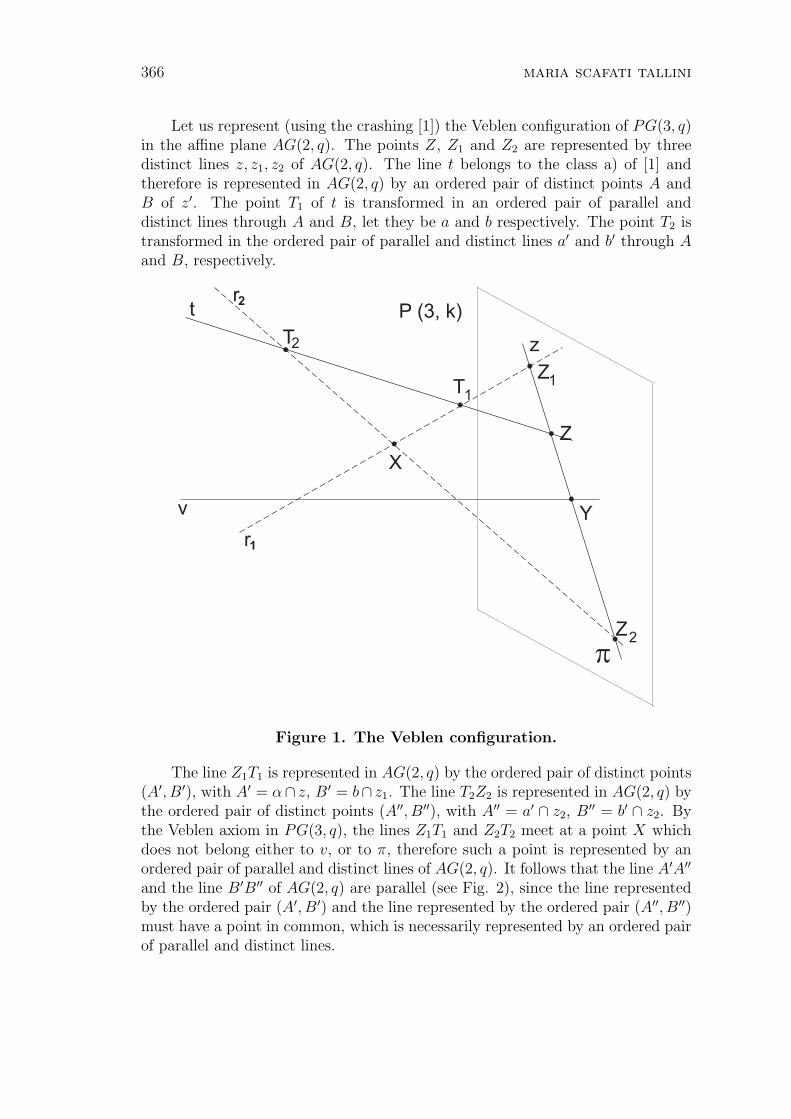
366 maria scafati tallini
Let us represent (using the crashing [1]) the Veblen configuration of PG(3, q)in the affine plane AG(2, q). The points Z, Z1 and Z2 are represented by threedistinct lines z, z1, z2 of AG(2, q). The line t belongs to the class a) of [1] andtherefore is represented in AG(2, q) by an ordered pair of distinct points A andB of z′. The point T1 of t is transformed in an ordered pair of parallel anddistinct lines through A and B, let they be a and b respectively. The point T2 istransformed in the ordered pair of parallel and distinct lines a′ and b′ through Aand B, respectively.
p
TZ
Z
Y
Z
X
P (3, k)
T
11
2
2 z
t
v
r
r
2
1
Figure 1. The Veblen configuration.
The line Z1T1 is represented in AG(2, q) by the ordered pair of distinct points(A′, B′), with A′ = α∩ z, B′ = b∩ z1. The line T2Z2 is represented in AG(2, q) bythe ordered pair of distinct points (A′′, B′′), with A′′ = a′ ∩ z2, B′′ = b′ ∩ z2. Bythe Veblen axiom in PG(3, q), the lines Z1T1 and Z2T2 meet at a point X whichdoes not belong either to v, or to π, therefore such a point is represented by anordered pair of parallel and distinct lines of AG(2, q). It follows that the line A′A′′
and the line B′B′′ of AG(2, q) are parallel (see Fig. 2), since the line representedby the ordered pair (A′, B′) and the line represented by the ordered pair (A′′, B′′)must have a point in common, which is necessarily represented by an ordered pairof parallel and distinct lines.
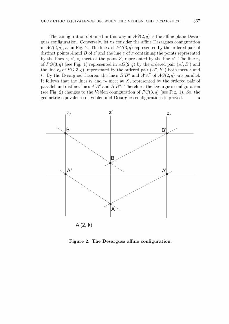
geometric equivalence between the veblen and desargues ... 367
The configuration obtained in this way in AG(2, q) is the affine plane Desar-gues configuration. Conversely, let us consider the affine Desargues configurationin AG(2, q), as in Fig. 2. The line t of PG(3, q) represented by the ordered pair ofdistinct points A and B of z′ and the line z of π containing the points representedby the lines z, z′, z2 meet at the point Z, represented by the line z′. The line r1
of PG(3, q) (see Fig. 1) represented in AG(2, q) by the ordered pair (A′, B′) andthe line r2 of PG(3, q), represented by the ordered pair (A′′, B′′) both meet z andt. By the Desargues theorem the lines B′B′′ and A′A′′ of AG(2, q) are parallel.It follows that the lines r1 and r2 meet at X, represented by the ordered pair ofparallel and distinct lines A′A′′ and B′B′′. Therefore, the Desargues configuration(see Fig. 2) changes to the Veblen configuration of PG(3, q) (see Fig. 1). So, thegeometric equivalence of Veblen and Desargues configurations is proved.
zz’z
A
A (2, k)
A’A”
B
B’B”
12
Figure 2. The Desargues affine configuration.

368 maria scafati tallini
2. The three stars theorem in PG(3, q) and its equivalencewith the Pappus–Pascal theorem in the affine plane AG(2, q)
Theorem 1. The ”three stars theorem”. Let PG(3, q) be the projective threedimensional space over the field k. Let v be a line of PG(3, q) and let π be a planenot through v meeting v at a point Y . Let U1 and U2 be two points of v, distinctbetween them and from Y . Let A1 and A2 be two distinct points of π such thatthe line A1A2 = d does not contain Y . Let s1, s2, s3 be three lines of π throughA1 distinct between them and from d and not through Y . Let s′1, s
′2, s
′3 be three
lines of π not through A2, distinct between them and from d and not through Y .Denoting by γ(Ui, sj) the plane through Ui and the line sj (i = 1, 2, j = 1, 2, 3),assume that the following two conditions are satisfied:
1) The planes γ(U1, s1), γ(U2, s2), γ(U1, s′2) and γ(U2, s
′1) belong to a star.
2) The planes γ(U1, s2), γ(U2, s3), γ(U1, s′3) and γ(U2, s
′2) belong to a star
(see Fig. 3).
Then, the four planes γ(U1, s3), γ(U2, s1), γ(U1, s′1) and γ(U2, s
′3) belong to a star.
U
s
s’
s
s’
s
s’
A
A
Uv y v
d
1
1
1
3
3
2
2
1
2
2
l
l’
p
Figure 3.

geometric equivalence between the veblen and desargues ... 369
Proof. Let r1 and r2 be the distinct lines of AG(2, q) representing the points A1
and A2, respectively (see [1]). Such lines are not parallel, since the line d does notpass through Y and so they meet at a point D. The lines s1, s2, s3 are representedin AG(2, q), by three pencils of lines with centres at D1, D2, D3, respectively, whichare distinct between them and from D and all contained in r1.
Similarly, the lines s′1, s′2, s
′3 are represented in AG(2, q) by three pencils of
lines with centres D′1, D
′2, D
′3, respectively, all contained in r2. We remark that
condition 1) is equivalent to the incidence of the lines ` = γ(U1, s1) ∩ γ(U2, s2)and `′ = γ(U1, s
′2) ∩ γ(U2, s
′1). Now, let us prove that the line `, which belongs to
the class a) of [1], in the crashing is represented by the ordered pair of distinctpoints (D1, D2). For, let S1 be a point of s1, distinct from s1 ∩ s2 and let t bethe line U1S1. Such a line t meets the line f of the class a), represented by thepair (D1, D2), since the dotted line t (which belongs to the class e) meets f at thepoint represented by the ordered pair (h1, h
′1), where h1 is the line representing
S1 and h′1 is the line through D2 and parallel to h1.
D
D’
D
O
D’
2
2
3
3
D
D’
1
2
1
1
p
p
Figure 4.
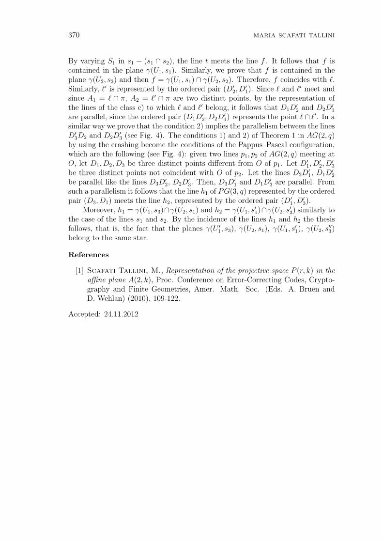
370 maria scafati tallini
By varying S1 in s1 − (s1 ∩ s2), the line t meets the line f . It follows that f iscontained in the plane γ(U1, s1). Similarly, we prove that f is contained in theplane γ(U2, s2) and then f = γ(U1, s1) ∩ γ(U2, s2). Therefore, f coincides with `.Similarly, `′ is represented by the ordered pair (D′
2, D′1). Since ` and `′ meet and
since A1 = ` ∩ π, A2 = `′ ∩ π are two distinct points, by the representation ofthe lines of the class c) to which ` and `′ belong, it follows that D1D
′2 and D2D
′1
are parallel, since the ordered pair (D1D′2, D2D
′1) represents the point `∩ `′. In a
similar way we prove that the condition 2) implies the parallelism between the linesD′
3D2 and D2D′3 (see Fig. 4). The conditions 1) and 2) of Theorem 1 in AG(2, q)
by using the crashing become the conditions of the Pappus–Pascal configuration,which are the following (see Fig. 4): given two lines p1, p2 of AG(2, q) meeting atO, let D1, D2, D3 be three distinct points different from O of p1. Let D′
1, D′2, D
′3
be three distinct points not coincident with O of p2. Let the lines D2D′1, D1D
′2
be parallel like the lines D3D′2, D2D
′3. Then, D3D
′1 and D1D
′3 are parallel. From
such a parallelism it follows that the line h1 of PG(3, q) represented by the orderedpair (D3, D1) meets the line h2, represented by the ordered pair (D′
1, D′3).
Moreover, h1 = γ(U1, s3)∩γ(U2, s1) and h2 = γ(U1, s′1)∩γ(U2, s
′3) similarly to
the case of the lines s1 and s2. By the incidence of the lines h1 and h2 the thesisfollows, that is, the fact that the planes γ(U ′
1, s3), γ(U2, s1), γ(U1, s′1), γ(U2, s
′′3)
belong to the same star.
References
[1] Scafati Tallini, M., Representation of the projective space P (r, k) in theaffine plane A(2, k), Proc. Conference on Error-Correcting Codes, Crypto-graphy and Finite Geometries, Amer. Math. Soc. (Eds. A. Bruen andD. Wehlan) (2010), 109-122.
Accepted: 24.11.2012
italian journal of pure and applied mathematics – n. 29−2012 (371−386) 371
THREE REPRESENTATIONS OF A HYPERBOLIC QUADRICOF PG(3, q) IN AG(2, q)
Maria Scafati Tallini
Summary. We construct three different representations of a hyperbolic quadric of aprojective Galois space PG(3,q) in the affine Galois plane AG(2, q). To do this, we usethe representation R, or R(U1, U2, π, 3) of the projective space P (r, k), over the fieldk, in the affine plane A(2, k), over the same field k, called also ”Crashing”, cited inthe bibliography [1]. Further applications of this representation are the constructionof maximal partial line spreads in PG, q even, a geometric proof of the equivalencebetween the Desargues and the Veblen theorems and a geometric proof of the equivalencebetween the Pappus-Pascal theorem and the ”Three stars theorem”. Those results willsoon appear.
1. First representation
Theorem 1. Theorem of the hyperbola and the hyperbolic quadric. LetPG(3, q) be the projective space of dimension three over the Galois field GF (q),let AG(2, q) be the affine plane over the same field and let R be an R(U1, U2, π, 3)-representation of PG(3, q), as in [1]. Let I be a hyperbola of AG(2, q) and let t1and t2 be the asymptots of I. Let T1 and T2 be the points of π represented throughR by the lines t1 and t2 of AG(2, q), respectively. For any point X of I, let X1
be the point common to t1 and to the line through X, parallel to t2, let X2 be thepoint common to the line t2 and to the line through X parallel to t1, let `X be theline of PG(3, q) represented through R, by the ordered pair (X1, X2) and, finally,let `X be the line of PG(3, q) represented through R by the ordered pair (X2, X1).Then, the following sets of PG(3, q):
R = `XX∈I ∪ U1T2, U2T1,R = `XX∈I ∪ U1T1, U2T2,
where UiTj, i, j = 1, 2, denotes the line of PG(3, q) through the points Ui and Tj,are the two reguli of a hyperbolic quadric of PG(3, q) meeting π at a non-degenerateconic, admitting v as a secant line.
Proof. Let PG(3, q) be the three dimensional projective space over GF (q),let AG(2, q) be the affine plane over GF (q) and let R be an R(U1, U2, π, 3)-representation of PG(3, q). Let I be a hyperbola of AG(2, q), let t1 and t2 be
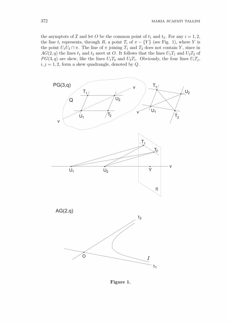
372 maria scafati tallini
the asymptots of I and let O be the common point of t1 and t2. For any i = 1, 2,the line ti represents, through R, a point Ti of π − Y (see Fig. 1), where Y isthe point U1U2 ∩ π. The line of π joining T1 and T2 does not contain Y , since inAG(2, q) the lines t1 and t2 meet at O. It follows that the lines U1T1 and U2T2 ofPG(3, q) are skew, like the lines U1T2 and U2T1. Obviously, the four lines UiTj,i, j = 1, 2, form a skew quadrangle, denoted by Q.
p
v
v
v
vT
T
T
T
U
Y
U
U
U
T
T
PG(3,q)
Q
1
1
2
1
2
U2
1
1
2
U1
2
2
AG(2,q)
t
O
t
1
2
I
Figure 1.
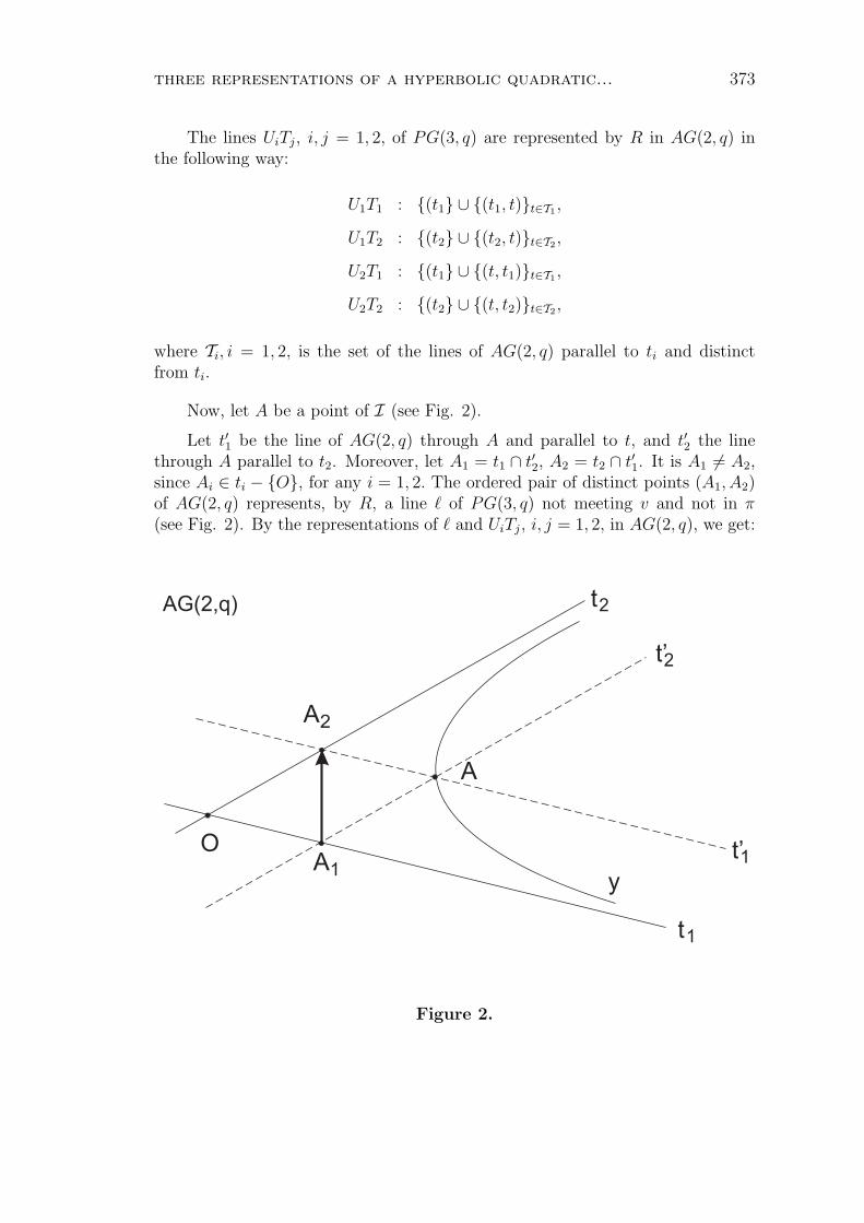
three representations of a hyperbolic quadratic... 373
The lines UiTj, i, j = 1, 2, of PG(3, q) are represented by R in AG(2, q) inthe following way:
U1T1 : (t1 ∪ (t1, t)t∈T1 ,
U1T2 : (t2 ∪ (t2, t)t∈T2 ,
U2T1 : (t1 ∪ (t, t1)t∈T1 ,
U2T2 : (t2 ∪ (t, t2)t∈T2 ,
where Ti, i = 1, 2, is the set of the lines of AG(2, q) parallel to ti and distinctfrom ti.
Now, let A be a point of I (see Fig. 2).
Let t′1 be the line of AG(2, q) through A and parallel to t, and t′2 the linethrough A parallel to t2. Moreover, let A1 = t1 ∩ t′2, A2 = t2 ∩ t′1. It is A1 6= A2,since Ai ∈ ti − O, for any i = 1, 2. The ordered pair of distinct points (A1, A2)of AG(2, q) represents, by R, a line ` of PG(3, q) not meeting v and not in π(see Fig. 2). By the representations of ` and UiTj, i, j = 1, 2, in AG(2, q), we get:
t1
t2
t’2
t’1O
A
A
2
A1
AG(2,q)
y
Figure 2.
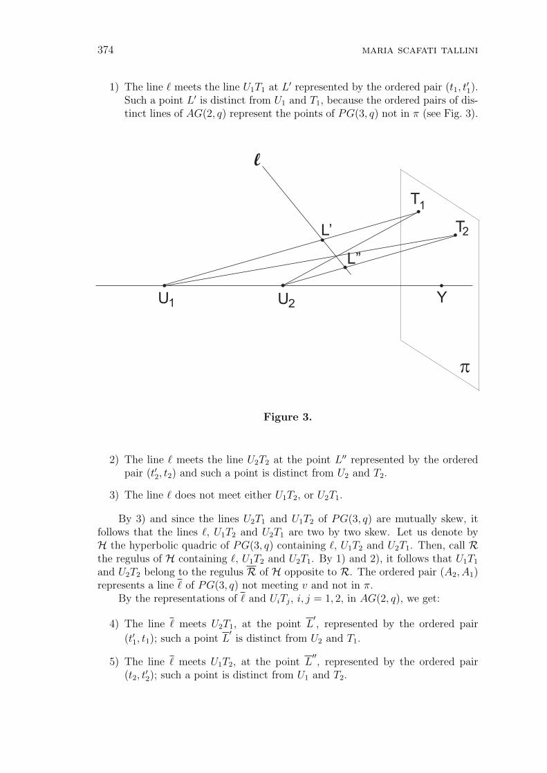
374 maria scafati tallini
1) The line ` meets the line U1T1 at L′ represented by the ordered pair (t1, t′1).
Such a point L′ is distinct from U1 and T1, because the ordered pairs of dis-tinct lines of AG(2, q) represent the points of PG(3, q) not in π (see Fig. 3).
p
T
L’
L”
Y
T
1
U2U1
2
l
Figure 3.
2) The line ` meets the line U2T2 at the point L′′ represented by the orderedpair (t′2, t2) and such a point is distinct from U2 and T2.
3) The line ` does not meet either U1T2, or U2T1.
By 3) and since the lines U2T1 and U1T2 of PG(3, q) are mutually skew, itfollows that the lines `, U1T2 and U2T1 are two by two skew. Let us denote byH the hyperbolic quadric of PG(3, q) containing `, U1T2 and U2T1. Then, call Rthe regulus of H containing `, U1T2 and U2T1. By 1) and 2), it follows that U1T1
and U2T2 belong to the regulus R of H opposite to R. The ordered pair (A2, A1)represents a line ` of PG(3, q) not meeting v and not in π.
By the representations of ` and UiTj, i, j = 1, 2, in AG(2, q), we get:
4) The line ` meets U2T1, at the point L′, represented by the ordered pair
(t′1, t1); such a point L′is distinct from U2 and T1.
5) The line ` meets U1T2, at the point L′′, represented by the ordered pair
(t2, t′2); such a point is distinct from U1 and T2.
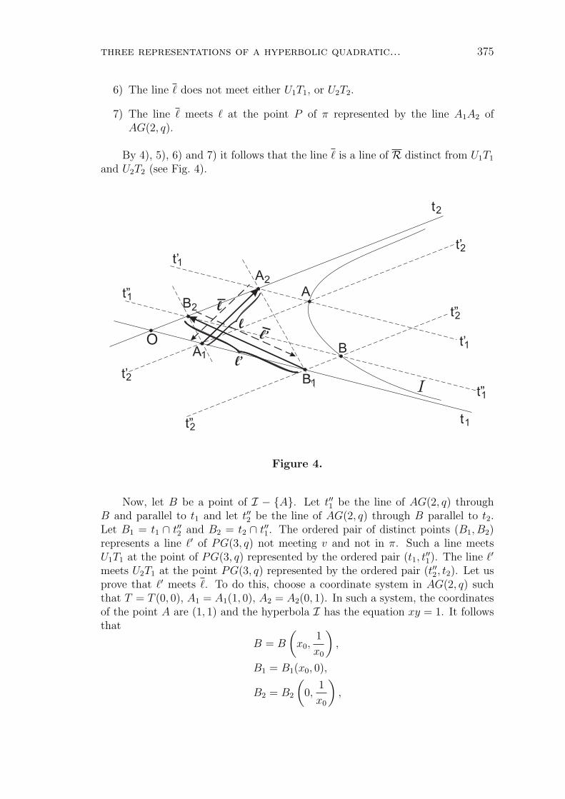
three representations of a hyperbolic quadratic... 375
6) The line ` does not meet either U1T1, or U2T2.
7) The line ` meets ` at the point P of π represented by the line A1A2 ofAG(2, q).
By 4), 5), 6) and 7) it follows that the line ` is a line of R distinct from U1T1
and U2T2 (see Fig. 4).
t2
t1t”
t”
2
2
t’2
t’2t’1
t”
t”
1
1
t’1
A
A
2
1
1
A
B
B
B2
l
l’
l
l’O
I
Figure 4.
Now, let B be a point of I − A. Let t′′1 be the line of AG(2, q) throughB and parallel to t1 and let t′′2 be the line of AG(2, q) through B parallel to t2.Let B1 = t1 ∩ t′′2 and B2 = t2 ∩ t′′1. The ordered pair of distinct points (B1, B2)represents a line `′ of PG(3, q) not meeting v and not in π. Such a line meetsU1T1 at the point of PG(3, q) represented by the ordered pair (t1, t
′′1). The line `′
meets U2T1 at the point PG(3, q) represented by the ordered pair (t′′2, t2). Let usprove that `′ meets `. To do this, choose a coordinate system in AG(2, q) suchthat T = T (0, 0), A1 = A1(1, 0), A2 = A2(0, 1). In such a system, the coordinatesof the point A are (1, 1) and the hyperbola I has the equation xy = 1. It followsthat
B = B
(x0,
1
x0
),
B1 = B1(x0, 0),
B2 = B2
(0,
1
x0
),
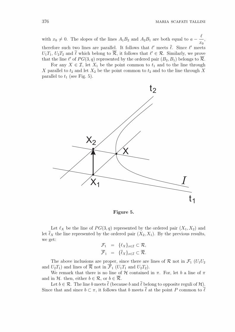
376 maria scafati tallini
with x0 6= 0. The slopes of the lines A1B2 and A2B1 are both equal to a − `
x0
,
therefore such two lines are parallel. It follows that `′ meets `. Since `′ meetsU1T1, U2T2 and ` which belong to R, it follows that `′ ∈ R. Similarly, we provethat the line `′ of PG(3, q) represented by the ordered pair (B2, B1) belongs to R.
For any X ∈ I, let X1 be the point common to t1 and to the line throughX parallel to t2 and let X2 be the point common to t2 and to the line through Xparallel to t1 (see Fig. 5).
t1
t2
X
X
2
X1I
Figure 5.
Let `X be the line of PG(3, q) represented by the ordered pair (X1, X2) andlet `X the line represented by the ordered pair (X2, X1). By the previous results,we get:
F1 = `Xx∈I ⊂ R,
F1 = `Xx∈I ⊂ R.
The above inclusions are proper, since there are lines of R not in F1 (U1U2
and U2T1) and lines of R not in F1 (U1T1 and U2T2).We remark that there is no line of H contained in π. For, let b a line of π
and in H. then, either b ∈ R, or b ∈ R.Let b ∈ R. The line b meets ` (because b and ` belong to opposite reguli ofH).
Since that and since b ⊂ π, it follows that b meets ` at the point P common to `

three representations of a hyperbolic quadratic... 377
and π, represented by R in AG(2, q) by the line A1A2. But such a point P belongsalso to the line b. Therefore, ` and b have P in common. Since ` and b are linesof the same regulus R of H, it follows b = `: a contradiction, since ` is not a lineof π, while b ⊂ π. The contradiction proves that b /∈ R. Similarly, we prove thatb /∈ R. So, we get a contradiction, because from b ⊂ H, it follows that b ∈ R∪R.The contradiction proves that there is no line of H contained in π. So, the remarkis proved.
From this remark it follows that H meets π at a non-degenerate conic. Ob-viously, every line of H is a line of R not meeting v, while every line of F is a lineof R not meeting v.
Now, let us prove that every line of R not meeting v is a line of F .Let ˜ be a line of R not meeting v. Since ˜ does not meet v and, since ˜ is
not a line of π (we already proved that no line of H is contained in π), it follows
that ˜ is represented by an ordered pair (L1, L2) of distinct points of AG(2, q).
The line ˜, which belongs to R, meets U1T1, U2T2 and `, which belong to R. Bythe representations of ˜, U1T1 and U2T2 and since ˜meets U1T1 and U2T2, we get
L1 ∈ t1, L2 ∈ t2.
We remark that L1 6= O. In fact, if L1 = O, the distinct points L1 and L2 belongboth to t2 and ˜ contains T2. It follows that ˜ = U1T2, since ˜∈ R, U1T2 ∈ R,T2 ∈ ˜, T2 ∈ U1T2: a contradiction, since ˜ does not meet v, while U1T2 meets vand U1. The contradiction proves the remark. Similarly, we prove that L2 6= O.
By the above remark and since L1 ∈ t1, L2 ∈ t2, it follows
L1 ∈ t1 − O, L2 ∈ t2 − O.
By the previous results, it follows immediately that L1 6= A2, L2 6= A1.As ˜ meets `, it follows that in AG(2, q) the line L1A2 is parallel to L2A1
(maybe coinciding with it). Let L be the point of AG(2, q) common to the linethrough L2 parallel to t1 and to the line through L1 parallel to t2. Let us provethat L ∈ I. In the coordinate system that we chose before, let m be the slope ofthe lines parallel to A1L2 and A2L1. Such a slope does exist, since L1 ∈ t1 − Oand it is different from zero because L2 ∈ t2−O. The points L1 and L2 have co-
ordinates L1
(− 1
m, 0
), L2(0,−m). It follows that L has coordinates
(− 1
m,−m
)
and then L ∈ I (remember that in our coordinate system the hyperbola I has theequation xy = 1). By the above results and by the definition of F , it follows that˜∈ F . So, every line of R not meeting v is a line of F . So, the result is proved.Similarly, we prove that every line of R not meeting v is a line of F . It followsthat all the lines of F coincide with the lines of R not meeting v, while the linesof F coincide with the lines of R not meeting v. We remark that the lines U2T2
and U2T1 coincide with the lines of R meeting v. For, U1T2 and U2T1 are lines ofR meeting v. Conversely, every line of R meeting v coincides either with U1T2,or with U2T1. For, let `R be a line of R meeting v distinct from U1T2 and U2T1.Then, the point L = `R ∩ v is distinct from either U1, or U2. Then the line v,

378 maria scafati tallini
having three distinct points in common with H, is a line of H. It follows v ∈ R,since v meets `R, U1T2 and U2T1, belonging to R. The line v meets also U2T2 ∈ R.It follows that v = U2T2, a contradiction, since T2 6= Y . The contradiction provesthat no line of R meeting v and distinct from U1T2 and U2T1 exists, whence everyline of R meeting v coincides either with U1T2, or with U2T1. So, the remarkis proved. Similarly, we prove that U1T1 and U2T2 coincide with the lines of Rmeeting v. By the above arguments, it follows that
R = F ∪ U1T2, U2T1,R = F ∪ U1T1, U2T2.
As all the hyperbolic quadrics of PG(3, q) are equivalent, it follows that forevery hyperbolic quadric H of PG(3, q) there is a representation R(U1, U2, π, 3) ofPG(3, q) which represents H by a hyperbola of AG(2, q).
2. Second representation
Let AG(2, q) be the affine plane over the Galois field GF (q). In AG(2, q), let t1and t2 be two distinct lines meeting at a point O. Let A be a point of t1 − O(see Fig. 6), let B be a point of t2−O and, finally, let t3 be the line through Aand B.
l
l’
r
T
t
t’ b’
b”
t
t
t
tt
t
t
T
B
L’
L’
L
L
T
T
N
A0
1
3
2
1
2
2
1
4
2
3
M
B
A2
1
2
1
4
T
M
M
Figure 6.
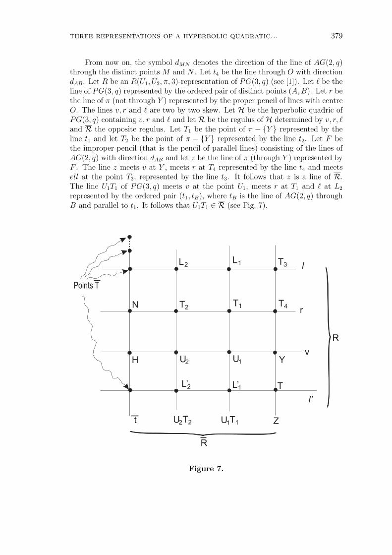
three representations of a hyperbolic quadratic... 379
From now on, the symbol dMN denotes the direction of the line of AG(2, q)through the distinct points M and N . Let t4 be the line through O with directiondAB. Let R be an R(U1, U2, π, 3)-representation of PG(3, q) (see [1]). Let ` be theline of PG(3, q) represented by the ordered pair of distinct points (A,B). Let r bethe line of π (not through Y ) represented by the proper pencil of lines with centreO. The lines v, r and ` are two by two skew. Let H be the hyperbolic quadric ofPG(3, q) containing v, r and ` and let R be the regulus of H determined by v, r, `and R the opposite regulus. Let T1 be the point of π − Y represented by theline t1 and let T2 be the point of π − Y represented by the line t2. Let F bethe improper pencil (that is the pencil of parallel lines) consisting of the lines ofAG(2, q) with direction dAB and let z be the line of π (through Y ) represented byF . The line z meets v at Y , meets r at T4 represented by the line t4 and meetsell at the point T3, represented by the line t3. It follows that z is a line of R.The line U1T1 of PG(3, q) meets v at the point U1, meets r at T1 and ` at L2
represented by the ordered pair (t1, tB), where tB is the line of AG(2, q) throughB and parallel to t1. It follows that U1T1 ∈ R (see Fig. 7).
l
r
v
l’
L’ L’
L
T
T
L
T
T
U
U
R
R
U
U
Y
T
Zt
T
TN
H
2 1
1
1
1
2
2
2
2
2
1
1
3
4
Points T
Figure 7.

380 maria scafati tallini
Now, let M1 and M2 be two points of AG(2, q) mutually distinct and suchthat M1 ∈ t1 − O, M2 ∈ t2 − O, dM1M2 = dAB. Let t be the line of AG(2, q)through M1 and M2. Let `′ be the line of PG(3, q) represented by the ordered pair(M1,M2). The line `′ meets z at T , represented by the line t, meets U1T1 at L′1,represented by the ordered pair (t1, tM2), where tM2 is the line of AG(2, q) throughM2 and parallel to t1, meeting U2T2 at the point L′2, represented by the orderedpair (tM1 , t2), where tM1 is the line of AG(2, q) through M1 and parallel to t2. Itfollows that `′ ∈ R. By the above arguments it follows that every ordered pairof distinct points (M1,M2), with M1 ∈ t1 − O, M2 ∈ t2 − O, dM1M2 = dAB,represents a line of R, distinct from v and r. Conversely, let m ∈ R−v, r. Theline m is not a line of π, since m and r are skew and r is a line of π. It follows thatm is represented by an ordered pair of distinct points (M1,M2). The line m, as aline of R, meets U1T1, U2T2 and z, which are lines of R. Since m meets z (at pointdistinct from Y ), it follows that dM1M2 = dAB. Since m meets U1T1, it followsthat M1 ∈ T1, while, since m meets U2T2, it follows that M2 ∈ t2. Moreover, byM1 6= M2, dM1M2 = dAB and since neither t1, nor t2 have the direction dAB, itfollows that M1 ∈ t1 − O and M2 ∈ t2 − O. By the previous arguments, itfollows that every line of R− v, r is represented by an ordered pair of distinctpoints (M1, M2), with M1 ∈ t1 − O, M2 ∈ t2 − O, dM1M2 = dAB. So, weprove that the ordered pairs of distinct points (M1,M2), with M1 ∈ t1 − O,M2 ∈ t2 − O, dM1M2 = dAB, represent exactly all the lines of R− v, r. If wedenote by `M1M2 the line of PG(3, q) represented in AG(2, q) by the ordered pairof distinct points (M1,M2), we get
R = v, r ∪ `M1M2 : M1 ∈ t1 − O,M2 ∈ t2 − O, dM1M2 = dAB.
Now, let α be a plane of PG(3, q) containing v but not through U1T1, U2T2
and z. Such a plane α is tangent to H at a point H ∈ v−Y, U1, U2 and containstherefore the line t of R through H. Moreover, α is spanned in AG(2, q) by adirection d′ distinct from dAB and distinct either from the direction of t1, or thatof t2. Consider the points of t−H. They are the intersections of the lines of Rdistinct from v with the plane α. Such points are therefore represented as follows:
1) The point N = t∩r = α∩r is represented by the line t′ of AG(2, q) throughO and of direction d′.
2) Each point T of t−H, N is represented by an ordered pair (b′, b′′), whereb′ and b′′ are the lines of AG(2, q) with direction d′ and through the pointsM1,M2 respectively, with
M1 ∈ t1 − O, M2 ∈ t2 − O,dM1M2 = dAB.
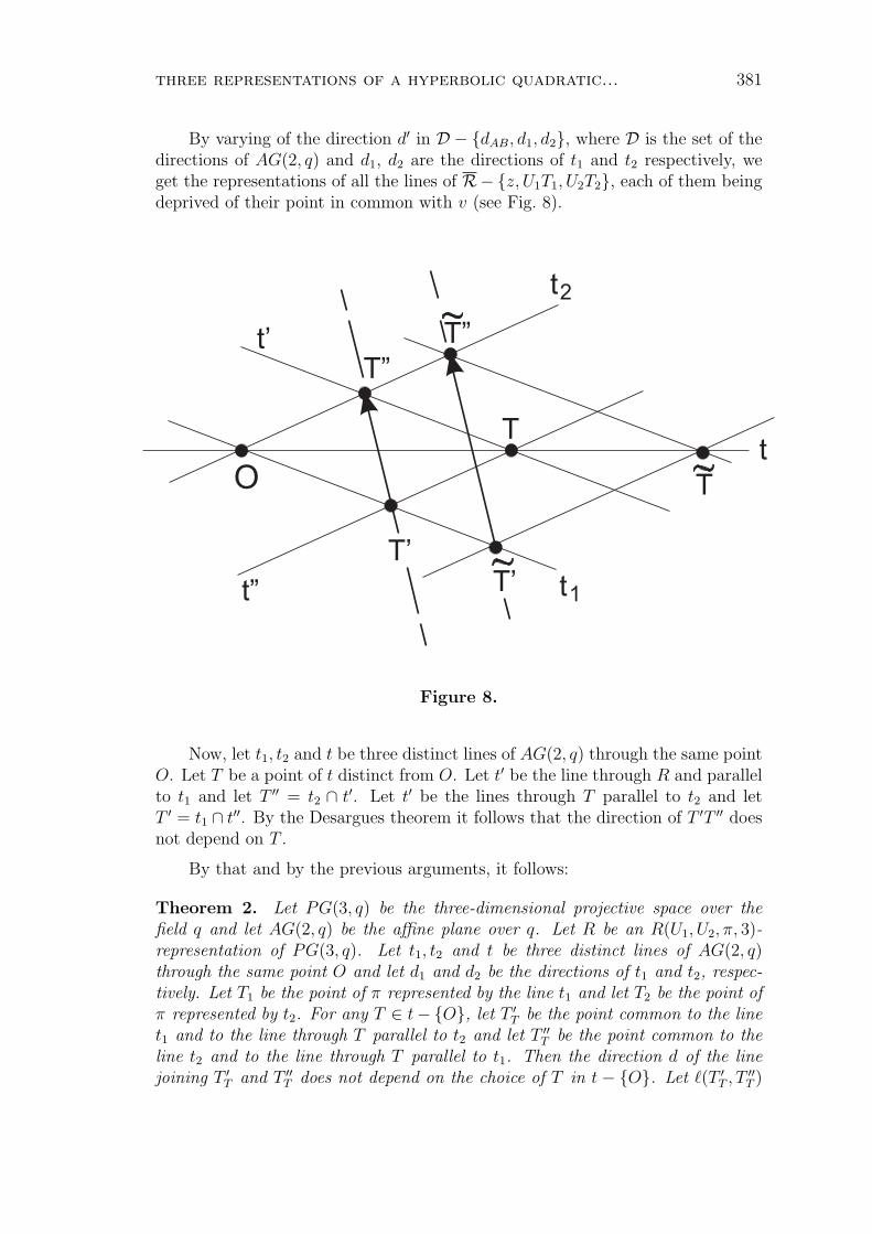
three representations of a hyperbolic quadratic... 381
By varying of the direction d′ in D − dAB, d1, d2, where D is the set of thedirections of AG(2, q) and d1, d2 are the directions of t1 and t2 respectively, weget the representations of all the lines of R−z, U1T1, U2T2, each of them beingdeprived of their point in common with v (see Fig. 8).
T”
T”
T
T’
T’
T
t
t
t
2
1
t’
t”
O
Figure 8.
Now, let t1, t2 and t be three distinct lines of AG(2, q) through the same pointO. Let T be a point of t distinct from O. Let t′ be the line through R and parallelto t1 and let T ′′ = t2 ∩ t′. Let t′ be the lines through T parallel to t2 and letT ′ = t1 ∩ t′′. By the Desargues theorem it follows that the direction of T ′T ′′ doesnot depend on T .
By that and by the previous arguments, it follows:
Theorem 2. Let PG(3, q) be the three-dimensional projective space over thefield q and let AG(2, q) be the affine plane over q. Let R be an R(U1, U2, π, 3)-representation of PG(3, q). Let t1, t2 and t be three distinct lines of AG(2, q)through the same point O and let d1 and d2 be the directions of t1 and t2, respec-tively. Let T1 be the point of π represented by the line t1 and let T2 be the point ofπ represented by t2. For any T ∈ t− O, let T ′
T be the point common to the linet1 and to the line through T parallel to t2 and let T ′′
T be the point common to theline t2 and to the line through T parallel to t1. Then the direction d of the linejoining T ′
T and T ′′T does not depend on the choice of T in t − O. Let `(T ′
T , T ′′T )
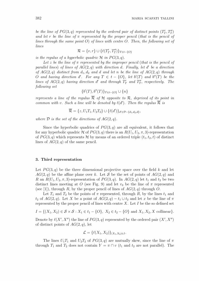
382 maria scafati tallini
be the line of PG(3, q) represented by the ordered pair of distinct points (T ′T , T ′′
T )and let r be the line of π represented by the proper pencil (that is the pencil oflines through the same point O) of lines with centre O. Then, the following set oflines
R = v, r ∪ `(T ′T , T ′′
T )T∈t−O
is the regulus of a hyperbolic quadric H in PG(3, q).Let z be the line of π represented by the improper pencil (that is the pencil of
parallel lines) of lines of AG(2, q) with direction d. Finally, let d′ be a directionof AG(2, q) distinct from d1, d2 and d and let n be the line of AG(2, q) throughO and having direction d′. For any T ∈ t − O, let b′(T ) and b′′(T ) be thelines of AG(2, q) having direction d′ and through T ′
T and T ′′T , respectively. The
following setb′(T ), b′′(T )T∈t−O ∪ n
represents a line of the regulus R of H opposite to R, deprived of its point incommon with v. Such a line will be denoted by `(d′). Then the regulus R is
R = z, U1T1, U2T2 ∪ `(d′)d′∈D−d1,d2,d,
where D is the set of the directions of AG(2, q).
Since the hyperbolic quadrics of PG(3, q) are all equivalent, it follows thatfor any hyperbolic quadric H of PG(3, q) there is an R(U1, U2, π, 3)-representationof PG(3, q) which represents H by means of an ordered triple (t1, t2, t) of distinctlines of AG(2, q) of the same pencil.
3. Third representation
Let PG(3, q) be the three dimensional projective space over the field k and letAG(2, q) be the affine plane over k. Let S be the set of points of AG(2, q) andR an R(U1, U2, π, 3)-representation of PG(3, q). In AG(2, q) let t1 and t2 be twodistinct lines meeting at O (see Fig. 9) and let r0 be the line of π represented(see [1]), through R, by the proper pencil of lines of AG(2, q) through O.
Let T1 and T2 be the points of π represented, through R, by the lines t1 andt2 of AG(2, q). Let X be a point of AG(2, q) − t1 ∪ t2 and let x be the line of πrepresented by the proper pencil of lines with centre X. Let I be the so defined set
I = (X1, X2) ∈ S ×S : X1 ∈ t1 − O, X2 ∈ t2 − O and X1, X2, X collinear.Denote by `(X ′, X ′′) the line of PG(3, q) represented by the ordered pair (X ′, X ′′)of distinct points of AG(2, q), let
L = `(X1, X2)(X1,X2)∈I .
The lines U1T1 and U2T2 of PG(3, q) are mutually skew, since the line of πthrough T1 and T2 does not contain Y = π ∩ v (t1 and t2 are not parallel). The
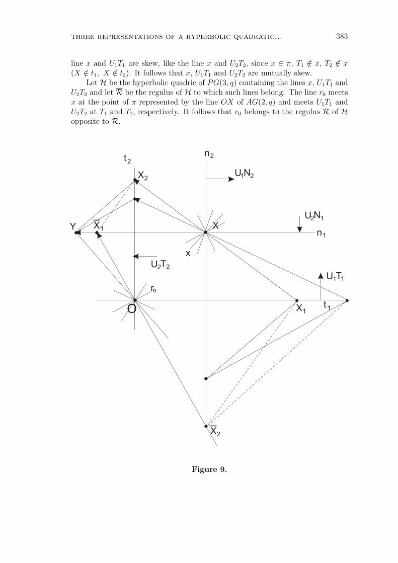
three representations of a hyperbolic quadratic... 383
line x and U1T1 are skew, like the line x and U2T2, since x ∈ π, T1 /∈ x, T2 /∈ x(X /∈ t1, X /∈ t2). It follows that x, U1T1 and U2T2 are mutually skew.
Let H be the hyperbolic quadric of PG(3, q) containing the lines x, U1T1 andU2T2 and let R be the regulus of H to which such lines belong. The line r0 meetsx at the point of π represented by the line OX of AG(2, q) and meets U1T1 andU2T2 at T1 and T2, respectively. It follows that r0 belongs to the regulus R of Hopposite to R.
N
N
T
T
U
U
X
X
X
x
U
U
n
nt
t
Y
O
2
1
2
1
2
1
2
1
1
2
1
22
1
ro
X1
X2
Figure 9.
384 maria scafati tallini
Moreover, it is easy to check that every line of L meets x, U1T1 and U2T2.It follows that every line of L belongs to R. Now, let n1 and n2 be the lines ofAG(2, q) through X and parallel to t1 and t2, respectively. Then, let N1 and N2
be the points of π represented by the lines n1 and n2, respectively. The line U2N1
of PG(3, q) meets U2T2 at U2, U1T1 at the point represented by the ordered pair(t1, n1) and x and N1. It follows that U2N1 ∈ R. The line U1N2 meets U1T1 atU1, U2T2 at the point represented by the ordered pair (n2, t2) and x at N2. ThenU1N2 ∈ R. By the above arguments, it follows
E = r0, U1N2, U2N1 ∪ L ⊆ R.
Now, let us prove that every line of R is a line of E.
Proof. Assume that r′ is a line of R not in E. Then r′ is not in π, otherwiser0 ∩ r′ 6= ∅, while r′ and r0 are skew, since r and r0 are two distinct lines of R(r0 ∈ E, r′ ∈ E). The line r′ does not contain U1 and U2, since r′ is distinct fromU1N2 and U2N1 (U1N2 ∈ E, U2N1 ∈ E, r′ /∈ E). Remark that r′ does not meetv. For, M = r′ ∩ v. By U1 /∈ r′, U2 /∈ r′, it follows that M 6= U1, M 6= U2. Then,v contains the three distinct points M , U1 and U2 of H and then v is a line ofH. Since v meets U1T1 and U2T2, which belong to R, it follows that v ∈ R andthen v meets x ∈ R: a contradiction, because x does not pass through Y = π ∩ v(x is represented in AG(2, q) by the proper pencil of lines with centre X). Thecontradiction proves the remark. Therefore, r′ is a line of PG(3, q) not in π andnot meeting v. It follows that r′ is represented by an ordered pair of distinctpoints (X1, X2) of AG(2, q). By r′ ∈ R and x ∈ R, it follows that r′ ∩ x 6= ∅ andthen the line of AG(2, q) joining X1 and X2 contains X. By r′ ∈ R and U1T1 ∈ R,it follows that r′ ∩U1T1 6= ∅ and then X1 ∈ t1. By r′ ∈ R and U2T2 ∈ R it followsr′ ∩ U2T2 6= ∅ and then X2 ∈ r2. Moreover, we get X1 6= O, x2 6= O, that isX1 ∈ t1 − O, X2 ∈ t2 − O, since the points X1, X2 and X are collinear andX1 6= X2. Then X1 ∈ t1 − O, X2 ∈ t2 − O and X1, X2, X are collinear. Bythat, it follows (X1, X2) ∈ I and then r′ = `(X1, X2) ∈ L ⊂ E, so r′ ∈ E is acontradiction, since r′ /∈ E. The contradiction proves that every line of R belongsto E and then R ⊆ E. By that and by E ⊆ R it follows R = E, that is
R = r0, U1N2, U2N1 ∪ L.
Now, let I be the following set
I = (X2, X1) ∈ S×S : X1 ∈ n1−X, X2 ∈ n2−X, X1, X2 and O collinear.
LetL = `(X2, X1)(X2,X1)∈I .
In a similar way as before, we get
R = x, U1T1, U2T2 ∪ L.
So, the following theorem is proved.
three representations of a hyperbolic quadratic... 385
Theorem 3. Let PG(3, q) be the projective three-dimensional space over the fieldq, let AG(2, q) be the affine plane over q and let S be the set of points of AG(2, q)and R an R(U1, U2, π, 3)-representation of PG(3, q) (see [1]). In AG(2, q) let t1 andt2 be two distinct lines meeting at a point O and let r0 be the line of π represented,through R, by the proper pencil of lines of AG(2, q) with centre O. Let T1 andT2 be the points of π represented through R, by the lines t1 and t2 of AG(2, q)respectively. Let X be a point of AG(2, q) − (t1 ∪ t2) and let x be the line of πrepresented by the proper pencil of lines of AG(2, q) with centre X.
Let n1 and n2 be the lines of AG(2, q) through X and parallel to t1 and t2,respectively. Then, let N1 and N2 be the points of π represented through R, by thelines n1 and n2, respectively. Let I and I be the following sets:
I = (X1, X2) ∈ S×S : X1 ∈ t1 − O, X2 ∈ t2 − Oand X1, X2, X collinear,
I = (X2, X1) ∈ S×S : X1 ∈ n1 − X, X2 ∈ n2 − Xand X1, X2, O collinear.
Denote by `(X ′, X ′′) the line of PG(3, q) represented through R by the orderedpair of distinct points (X ′, X ′′) of AG(2, q).
LetL = `(X1, X2)(X1,X2)∈I ,
L = `(X2, X1)(X2,X1)∈I .
Then the following sets of lines or PG(3, q)
R = r0, U1N2, U2N1 ∪ L,
R = x, U1T1, U2T2 ∪ L,
are the two reguli of a hyperbolic quadric of PG(3, q) admitting the plane π astangent plane, the contact point being the point of π represented by the line OXof AG(2, q) and the line v being a secant line.
The above theorem allows us to represent in the plane AG(2, q) the reguliand then the points of a hyperbolic quadric H, deprived of two points which arenot represented. For, the line r0 is represented by the pencil of lines of AG(2, q)with centre O, the line x is represented by the pencil of lines of AG(2, q) withcentre X, the lines U1N2, U2N1, U1T1 U2T2 are represented as follows:
U1N2 − U1 : n2 ∪ n2, n : n parallel to n2 and distinct from n2,
U2N1 − U2 : n1 ∪ n, n1 : n parallel to n1 and distinct from n1,
U1T1 − U1 : t1 ∪ t1, t : t parallel to t1 and distinct from t1,
U2T2 − U2 : t2 ∪ t, t2 : t parallel to t2 and distinct from t2,
Since the hyperbolic quadrics are all equivalent in PG(3, q), it follows that for anyhyperbolic quadric H of PG(3, q) there is an R(U1, U2, π, 3)-representation whichallows us to represent H as in Theorem 3.

386 maria scafati tallini
Those three different representations of a hyperbolic quadric of PG(3, q) inAG(2, q) show a further application of the representation called also ”crashing”cited in the bibliography.
Bibliography
[1] Scafati Tallini, M., Representation of the projective space P (r, k) in theaffine plane A(2, k), Proc. Conference on Error-Correcting Codes, Crypto-graphy and Finite Geometries, Amer. Math. Soc. (Eds. A. Bruen andD. Wehlan) (2010), 109-122.
Accepted: 24.11.2012
italian journal of pure and applied mathematics – n. 29−2012 (387−394) 387
RECOGNITION OF A10 AND L4(4) BY TWO SPECIALCONJUGACY CLASS SIZES1
Yanheng Chen
School of Mathematics and StatisticsSouthwest UniversityChongqing 400715P.R. ChinaandSchool of Mathematics and StatisticsChongqing Three Gorges UniversityChongqing404100P.R. China
Guiyun Chen2
School of Mathematics and StatisticsSouthwest UniversityChongqing 400715P.R. Chinae-mail: [email protected]
math [email protected]
Abstract. It is well-known that A10 is the smallest (by order) nonabelian simple groupwith connected prime graph and L4(4) is the smallest nonabelian simple group of Lietype with connected prime graph. In 2009, A.V. Vasil’ev first dealt with the groups withconnected prime graph and proved that Thompson’s conjecture holds for A10 and L4(4)(see [1]). In this work, the authors characterize finite simple groups A10 and L4(4) bytheir orders and largest and smallest conjugacy class sizes greater than 1, and partiallygeneralize A.V. Vasil’ev’s work.
Keywords: finite simple groups, conjugacy class size, prime graph.
AMS Mathematics Subject Classification(2010): 20D08, 20D60.
1. Introduction
Throughout this paper, groups under consideration are finite. For any group G,π(G) denotes the set of prime divisors of |G|. We associate to π(G) a simplegraph called prime graph of G, denoted by Γ(G). Prime graph Γ(G) is defined as
1This work was supported by National Natural Science Foundation of China (Grant Nos.11171364, 11001226), Natural Science Foundation of Chongqing (Grant No. cstc2011jjA1495),Science and Technology Foundation of Chongqing Education Committee (Grant Nos. KJ110609,KJ111107) and Youth Foundation of Chongqing Three Gorges University (Grant Nos. 12QN-23and 12QN-24 ).
2Corresponding author.
388 yanheng chen, guiyun chen
follows: the vertex of Γ(G) is the set of all prime divisors of the order of G, twodistinct vertexes p and q are adjacent by edge if and only if there is an elementof order pq in G(see [10]). Denote the connected components of the prime graphby T (G) = πi(G)|1 6 i 6 t(G), where t(G) is the number of the prime graphcomponents of G. If the order of G is even, we always assume that 2 ∈ π1(G).In addition, for x ∈ G, clG(x) denotes the conjugacy class in G containing x andCG(x) denotes the centralizer of x in G. Let cs(G) = n ∈ N|G has a conjugacyclass C such that |C| = n. For p ∈ π(G), we denote Gp and Sylp(G) a Sylowp−subgroup of G and the set of all of its Sylow p−subgroups, respectively. Wealso denote Soc(G) the socle of G which is the subgroup generated by the set ofa minimal normal subgroups of G. The other notation and terminologies in thispaper are standard and the reader is referred to [8] if necessary. The second authorG.Y. Chen once worked on J.G. Thompson’s conjecture posed by J.G. Thompsonin 1980s, which is about characterizing finite simple groups by the set of lengthsof its conjugacy classes as following (ref. to [[9], Problem 12.38]):
Thompson’s conjecture. Let G be a finite group with Z(G) = 1 and L is afinite non-abelian simple group satisfying that cs(G) = cs(L), then G ' L.
In 1994, G.Y. Chen proved in his Ph.D. dissertation [3] that if G is a groupwith Z(G) = 1, and L a non-abelian simple group with non-connected primegraph such that cs(G) = cs(L), then G ' L (also ref. to [4], [5], [6]). In 2009,A.V. Vasil’ev first dealt with the groups with connected prime graph and provedthat Thompson’s conjecture holds for A10 and L4(4) (see [1]). In 2011, N. Ahan-jideh in [2] proved that Thompson’s conjecture is true for Ln(q). Recently,G.Y. Chen and J.B. Li contributed their interests on special class sizes of finitesimple groups, and characterize successfully sporadic simple groups (see J.B. Li’sPh.D. dissertation [15])and simple K3−groups (to prepared) by their orders andfew special class sizes greater than 1. In their papers, they provided two newways to characterize finite simple group by group order and largest class size, orsmallest class size greater than 1. More importantly, one of two methods doesn’tconsider about connection of prime graph of group. Thus it is may be effec-tive to deal with simple groups which have connected prime graph. In this paper,we focus our attention on simple groups A10 and L4(4) which have connected primegraphs, and characterize A10 and L4(4) by their orders, and largest and smallestconjugacy class sizes greater than 1, respectively. In addition, we partially genera-lize A.V. Vasil’ev’s work (see [1]) and prove that Thompson’s conjecture holds forA10 and L4(4) at the same time. That is the following theorem. For convenience,lcs(G) and scs(G) denote largest and smallest conjugacy class size greater than 1of group G, respectively.
Main Theorem. Let G be a group and L one of A10 and L4(4). Then G ' L ifand only if |G| = |L| and lcs(G) = lcs(L) and scs(G) = scs(L).
If Main Theorem is proved, then the following corollary holds, which provesThompson’s conjecture for A10 and L4(4).
Corollary. Thompson’s conjecture holds for finite simple group A10 and L4(4).
recognition of A10 and L4(4) by two special conjugacy class sizes389
Proof. Let G be a group and L one of A10 and L4(4). Under the hypothesisof Thompson’s conjecture, it is proved in [1] that |G| = |L|. Hence the corollaryfollows from Main Theorem.
2. Preliminaries
First, we generalize a simple fact which is used many times in G.Y. Chen andJ.B. Li’s works. It is important to prove our Main Theorem.
Lemma 2.1. Let G be a group, G = G/Z(G). N is a minimal normal subgroupof G, and N is the pre-image of N in G. If p ∈ π(N) for some p ∈ π(G) andNp ∈ Sylp(N) satisfying |Np| < scs(G), then N is not solvable.
Proof. Assume that N is solvable. Then N is an elementary abelian p−groupwith |N | = pt, t ≥ 1, and N is a nilpotent normal subgroup of G by the hypothesis.Hence Np is a normal subgroup of G, and Np is not a subgroup of Z(G). So thereexists an element x of Np − Z(G) satisfying that
1 < |clG(x)| = |G : CG(x)| ≤ |Np| < scs(G),
violating the hypothesis.
By Lemma 2.1, the fact can easily be obtained as a corollary following.
Corollary 2.2. Let G be a group, G = G/Z(G). If |Gp| < scs(G) for anyp ∈ π(G), then Soc(G) E G .Aut(Soc(G)).
Proof. Suppose that N is any minimal normal subgroup of G, and N is the pre-image of N in G. By the hypothesis, N satisfies that |Np| ≤ |Gp| < scs(G),so every minimal normal subgroup of G is not solvable by Lemma 2.1. LetS1, S2, . . . , Sk(k ≥ 1) be all minimal normal subgroup of G. Let M = Soc(G),hence M = Soc(G) = S1 × S2 × · · · × Sk and Si is a direct product of someisomorphic non-abelian simple groups for i = 1, 2, . . . , k. Now, we assert thatCG(M) = 1. If not, there exists a minimal normal subgroup S of G such thatS ≤ CG(M)
⋂M . Thus S is an abelian group, a contradiction. By N/C theorem,
we have M E G = G/CG(M) .Aut(M), as desired.
Lemma 2.3. Let K be a normal subgroup of a group G, and G = G/K. If x is theimage of an element x of G in G, and (|x|, |K|) = 1, then CG(x) = CG(x)K/K.In particular, if K = Z(G), then CG(x) = CG(x)/Z(G).
Proof. This is an immediate consequence of Theorem 1.6.2 in [14] or Lemma 5in [1]. For π(A10), π(L4(4)) ⊆ 2, 3, 5, 7, 17, we need to list all the non-abeliansimple groups L satisfying with π(L) ⊆ 2, 3, 5, 7, 17.Lemma 2.4. Let L be a non-abelian simple group. If π(L) ⊆ 2, 3, 5, 7, 17, thenL is isomorphic to one of simple groups of Table 1. Especially, 2, 3 ⊆ π(L),and if L 6= S6(2), S8(2), then π(Out(L)) ⊆ 2, 3.Proof. This is Lemma 2.5 in [7].
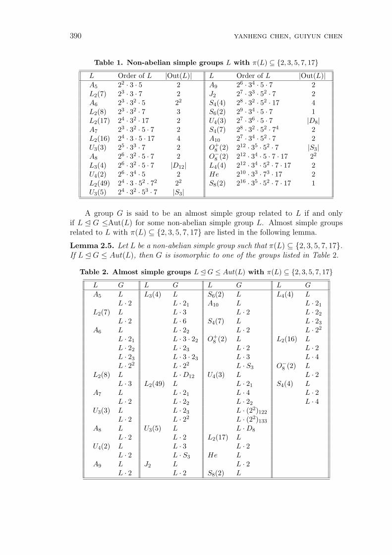
390 yanheng chen, guiyun chen
Table 1. Non-abelian simple groups L with π(L) ⊆ 2, 3, 5, 7, 17L Order of L |Out(L)| L Order of L |Out(L)|A5 22 · 3 · 5 2 A9 26 · 34 · 5 · 7 2L2(7) 23 · 3 · 7 2 J2 27 · 33 · 52 · 7 2A6 23 · 32 · 5 22 S4(4) 28 · 32 · 52 · 17 4L2(8) 23 · 32 · 7 3 S6(2) 29 · 34 · 5 · 7 1L2(17) 24 · 32 · 17 2 U4(3) 27 · 36 · 5 · 7 |D8|A7 23 · 32 · 5 · 7 2 S4(7) 28 · 32 · 52 · 74 2L2(16) 24 · 3 · 5 · 17 4 A10 27 · 34 · 52 · 7 2U3(3) 25 · 33 · 7 2 O+
8 (2) 212 · 35 · 52 · 7 |S3|A8 26 · 32 · 5 · 7 2 O−
8 (2) 212 · 34 · 5 · 7 · 17 22
L3(4) 26 · 32 · 5 · 7 |D12| L4(4) 212 · 34 · 52 · 7 · 17 2U4(2) 26 · 34 · 5 2 He 210 · 33 · 73 · 17 2L2(49) 24 · 3 · 52 · 72 22 S8(2) 216 · 35 · 52 · 7 · 17 1U3(5) 24 · 32 · 53 · 7 |S3|
A group G is said to be an almost simple group related to L if and onlyif L E G ≤Aut(L) for some non-abelian simple group L. Almost simple groupsrelated to L with π(L) ⊆ 2, 3, 5, 7, 17 are listed in the following lemma.
Lemma 2.5. Let L be a non-abelian simple group such that π(L) ⊆ 2, 3, 5, 7, 17.If L E G ≤ Aut(L), then G is isomorphic to one of the groups listed in Table 2.
Table 2. Almost simple groups L E G ≤ Aut(L) with π(L) ⊆ 2, 3, 5, 7, 17L G L G L G L G
A5 L L3(4) L S6(2) L L4(4) LL · 2 L · 21 A10 L L · 21
L2(7) L L · 3 L · 2 L · 22
L · 2 L · 6 S4(7) L L · 23
A6 L L · 22 L · 2 L · 22
L · 21 L · 3 · 22 O+8 (2) L L2(16) L
L · 22 L · 23 L · 2 L · 2L · 23 L · 3 · 23 L · 3 L · 4L · 22 L · 22 L · S3 O−
8 (2) LL2(8) L L ·D12 U4(3) L L · 2
L · 3 L2(49) L L · 21 S4(4) LA7 L L · 21 L · 4 L · 2
L · 2 L · 22 L · 22 L · 4U3(3) L L · 23 L · (22)122
L · 2 L · 22 L · (22)133
A8 L U3(5) L L ·D8
L · 2 L · 2 L2(17) LU4(2) L L · 3 L · 2
L · 2 L · S3 He LA9 L J2 L L · 2
L · 2 L · 2 S8(2) L

recognition of A10 and L4(4) by two special conjugacy class sizes391
Proof. All almost simple groups not related to L2(17), L2(16), S4(4), S8(2),O−
8 (2), L4(4), and He listed in Table 2 were given in Proposition 1 in [11]. Thoserelated to one of L2(17), L2(16), S4(4), S8(2), O−
8 (2), L4(4), and He are easilyobtained by an algorithm from [12].
Lemma 2.6. Let R = R1×· · ·×Rk, where Ri is a direct product of ni isomorphiccopies of a non-abelian simple group Hi, where Hi and Hj are not isomorphic ifi 6= j. Then Aut(R)'Aut(R1)×· · ·× Aut(Rk) and Aut(Ri)'(Aut(Hi)oSni
, wherein this wreath product Aut(Hi) appears in its right regular representation and thesymmetric group Sni
in its natural permutation representation. Moreover, theseisomorphisms induce outer automorphisms Out(R) 'Out(R1)×· · ·×Out(Rk) andOut(Ri)'(Out(Hi) o Sni
.
Proof. This is Theorem 3.3.20 in [13].
3. Proof of the Main Theorem
We divide the sufficient proof of Main Theorem into two lemmas.
Lemma 3.1. Let G be a group with |G| = 27 · 34 · 52 · 7. If lcs(G) = 24 · 34 · 52 · 7and scs(G) = 24 · 3 · 5. Then G ' A10.
Proof. It is clear that one has that Z(G) 6 CG(x) for any x ∈ G. Set x, andy ∈ G such that lcs(G) =|clG(x)|= 24 · 34 · 52 · 7 and scs(G) =|clG(y)|= 24 · 3 · 5.Since |G| = 27 · 34 · 52 · 7 and lcs(G) = 24 · 34 · 52 · 7, Z(G) is a proper subgroup ofG with |Z(G)| | 23 by the hypothesis. Thus 3, 5, and 7 6∈ π(Z(G)). ConsideringG = G/Z(G). For any prime p ∈ π(G), the order of Sylow p−subgroup ofG is less than scs(G). By Corollary 2.2, we know that every minimal normalsubgroup of G = G/Z(G) is non-solvable and Soc(G) E G ≤Aut(Soc(G)). LetM = Soc(G) and S1, S2, · · · , Sk(k ≥ 1) be all minimal normal subgroups of G,hence M = Soc(G) = S1 × S2 × · · · × Sk and Si is a direct product of someisomorphic non-abelian simple groups for i = 1, 2, . . . , k.
We assert that 3 ∈ π(M). Otherwise, M is a simple K3−group with π(M) =2, 5, 7. This is impossible by Table 1.
We assert that 5 ∈ π(M). Otherwise, M is a simple K3−group with π(M) =2, 3, 7 and 5 ∈ π(Out(G)). By Table 1, we find that M is isomorphic to oneof the following simple groups: L2(7), L2(8), and U3(3). By Lemma 2.4, we seethat |Out(L2(7))| = |Out(U3(3))| = 2, and |Out(L2(8))| = 3, a contradiction to5 ∈ π(Out(G)).
We also assert that 7∈π(M). Otherwise, π(M)=2, 3, 5 and 7∈π(Out(G)).By Table 1, M may be isomorphic to one of the following groups:
A5, A6, U4(2), A5 × A5, A5 × A6, and A6 × A6.
By Lemma 2.4 and Lemma 2.6, we see that outer automorphism groups of thesegroups are 2−groups, contradicting to 7 ∈ π(Out(G)). Hence 3, 5, 7 ⊆ π(M).By Table 1 again, M may be isomorphic to one of the following groups:
A7, A8, L3(4), A9, J2, A10, A5 × L2(7), A5 × L2(8), A5 × U3(3), A5 × A7,L2(7)× A6, and L2(8)× A6.
392 yanheng chen, guiyun chen
Now, let us recall that M E G ≤Aut(M). If M is isomorphic to one ofA7, A8, L3(4), A9, A5 ×L2(7), A5 ×L2(8), A5 ×U3(3), L2(7)×A6, and L2(8)×A6,then we have that 5 ‖ |G| by Table 1 and Lemma 2.6. Hence 5 ∈ π(Z(G)), acontradiction. If M is isomorphic to one of J2, and A5 × A7, then by the samereasoning 3 ∈ π(Z(G)), a contradiction.
Hence M ' A10 and G must be isomorphic to A10 by comparing the ordersof M and G, as claimed.
Lemma 3.2. Let G be a group with |G| = 212·34·52·7·17. If lcs(G) = 210·32·52·7·17and scs(G) = 32 · 5 · 7 · 17. Then G ' L4(4).
Proof. First, for any x ∈ G, Z(G) is contained in CG(x). By the hypothesis,there exist y, and z ∈ G such that scs(G)= |clG(y)| =32 · 5 · 7 · 17 and lcs(G)=|clG(z)| =210 ·32 ·52 ·7·17. Since |G| = 212 ·34 ·52 ·7·17, and lcs(G) = 210 ·32 ·52 ·7·17,we have that Z(G) is a proper subgroup of G of order dividing 36. Similar toLemma 3.1, Considering G = G/Z(G). For any prime p ∈ π(G), the order of Sylowp−subgroup of G is less than scs(G). Hence by Corollary 2.2, we know that everyminimal normal subgroup of G is non-solvable and Soc(G) E G ≤Aut(Soc(G)).Let M = Soc(G) and S1, S2, . . . , Sk(k ≥ 1) be all minimal normal subgroups ofG. Hence M = Soc(G) = S1 × S2 × · · · × Sk and Si is a direct product of someisomorphic non-abelian simple groups for i = 1, 2, . . . , k. Similar to the proofLemma 3.1, we prove 5, 7, and 17 ∈ π(M).
If 5 6∈ π(M), then 5 ∈ π(Out(M)). Applying Table 1 and possible order ofM , M may be isomorphic to one of the following groups:
L2(7), L2(8), L2(17), U3(3), L2(7)× L2(17), and L2(8)× L2(17).
By Lemmas 2.4 and 2.6, we see that outer automorphism groups of groups aboveare 2, 3−groups, a contradiction to 5 ∈ π(Out(M)). Therefore, 5 ∈ π(M).
If 7 6∈ π(M), then 7 ∈ π(Out(M)). By Table 1 and 5 ∈ π(M), M may beisomorphic to one of the following groups:
A5, A6, L2(16), U4(2), S4(4), A5 × A5, A5 × A6, A6 × A6, A5 × L2(17),A5 × L2(16), A6 × L2(17), and A6 × L2(16).
By Table 1 and Lemma 2.6, we see that outer automorphism groups of thesegroups are 2− groups, a contradiction. Hence 7 ∈ π(M).
If 17 6∈ π(M), then 17 ∈ π(Out(G)). By Table 1 and 5, 7 ⊆ π(M), M maybe isomorphic to one of the following groups:
A7, A8, L3(4), A9, J2, S6(2), A10, A5 × L2(7), A5 × L2(8), A5 × A7, A5 × A8,A5 × L3(4), A6 × L2(7), A6 × L2(8), A6 × A7, A6 × A8, A6 × L3(4),
and A5 × L2(7)× A6.
By Table 1 and Lemma 2.6, we know that 17 is not a prime divisor of outerautomorphism of those groups above, a contradiction. Hence 17 ∈ π(M). Forconvenience, we assume that 7 ∈ π(Si), and 17 ∈ π(Sj) for i, j ∈ 1, 2, · · · , k.
recognition of A10 and L4(4) by two special conjugacy class sizes393
If i 6= j, then Si and Sj are two non-isomorphic simple groups. By Table 1and possible order of M again, we see that M may be isomorphic to one of thefollowing groups:
L2(7)× L2(16), L2(7)× L2(17), L2(7)× S4(4), L2(8)× L2(16),L2(8)× L2(17), L2(8)× S4(4), A7 × L2(16), A7 × L2(17), U3(3)× L2(16),A8 × L2(16), A8 × L2(17), L3(4)× L2(16), L3(4)× L2(17),A5 × L2(7)× L2(16), A5 × L2(7)× L2(17), A5 × L2(8)× L2(16),and A6 × L2(7)× L2(16).
If M is isomorphic to one of the following groups:
L2(7)× L2(16), L2(7)× L2(17), ÃL2(8)× L2(16), U3(3)× L2(16), A8 × L2(17),L3(4)× L2(17), L2(8)× L2(17), A7 × L2(17), and A5 × L2(7)× L2(17),
then, by Table 1 and Lemma 2.6, we come to 5 ∈ π(Z(G)) by comparing theorders of M, G, and Aut(M), a contradiction.
If M ' L2(7)× S4(4), then
Aut(M) = Aut(L2(7))×AutS4(4)) = L2(7) · 2× S4(4) · 4by Lemma 2.6 and Table 2.
Recall that M E G ≤Aut(M), then |Z(G)| = 3 or 6. So there exists anelement w of order 7 in G such that CG(w)/Z(G) = CG(w) ≥ 〈w〉 × S4(4) byLemma 2.3, where w is the image of w in G. Hence |CG(w)| ≥ 28 · 33 · 52 · 7 · 17such that 1 < |clG(w)| < scs(G), a contradiction to minimality of scs(G).
If M ' L2(8) × S4(4), then by same way above we come to Aut(M) =L2(8) · 3× S4(4) · 4 such that |Z(G)| ≤ 2. So there exists an element w of order 7in G such that such that 1 < |clG(w)| < scs(G), a contradiction.
In a similar way used above, we can deal with the remaining cases of M , andcan always find an element of G such that its conjugacy class length is less thanscs(G), leading to a contradiction.
Hence i = j. Without loss of generality, assume that 7, and 17 ∈ π(S1). ThenS1 is a non-abelian simple group and isomorphic to O−
8 (2) or L4(4) by Table 1.Therefore k = 1, and M may be isomorphic to one of following groups: O−
8 (2),and L4(4).
If M ' O−8 (2), then, by Table 1 and Table 2, G ' O−
8 (2) or O−8 (2) · 2
and Aut(M) = O−8 (2) · 2. Comparing the orders of M, G, and Aut(M), we see
that |Z(G)| = 5 and G ' O−8 (2). If G is a split extension O−
8 (2) by Z(G), thenG = O−
8 (2)×Z(G). Therefore, by [8], there exists a non-central element w of order2 in G such that 1 < |clG(w)| < scs(G), leading to a contradiction. Hence G isnot a split extension O−
8 (2) by Z(G), which implies that 5 divides |Mult(O−8 (2))|,
a contradiction to |Mult(O−8 (2))| = 2 by [8].
Hence M ' L4(4) and so G must be isomorphic to L4(4) by |G| = |M |, asdesired.
Proof of the Main Theorem. The necessity is obvious by [8] and the sufficiencyfollows from Lemmas 3.1 and 3.2.
394 yanheng chen, guiyun chen
References
[1] Vasil’ev, A.V., On Thompson’s conjecture, Siberian Electronic Mathema-tical Reports, 6 (2009), 457-464.
[2] Ahanjideh, N., On Thompson’s conjecture for some finite simple groups,J. Algerba, 344 (2011), 205–228.
[3] Chen, G.Y., On Thompson’s Conjecture, Sichuan University, Chengdu,1994 (in Chinese).
[4] Chen, G.Y., On Thompson’s cconjecture for sporadic simple groups, Proc.China Assoc. Sci. and Tech. First Academic Annual Meeting of Youths,pp. 1-6, Chinese Sci. and Tech. Press, Beijing, 1992 (in Chinese).
[5] Chen, G.Y., On Thompson’s conjecture, J. Algebra, 185 (1996), 184-193.
[6] Chen, G.Y., Further reflections on Thompson’s conjecture, J. Algebra, 218(1999), 276-285.
[7] Zhang, L.C., Shi, W.J., Liu, X.F., A new characterization L4(4), ChineseAnnals of Mathematics, Series A, 30 (2009), 517-524 (in Chinese).
[8] Conway, J.H., Curtis, R.T., Norton, S.P., Parker, R.A., Wilson,R.A., Atlas of Finite Groups, Clarendon Press, Oxford, 1985.
[9] Khukhro, E.I., Mazurov, V.D., Unsolved Problems in Group Theory:The Kourovka Notebook, 17th edition, Sobolev Institute of Mathematics,Novosibirsk, 2010.
[10] Williams, J.S., Prime graph components of finite groups, J. Algebra, 69(1981), 487-513.
[11] Mazurov, V.D., Characterizations of finite groups by the set of orders oftheir elements, Algebra and Logic, 36 (1997), 23-32.
[12] Mazurov, V.D., The set of orders of elements in a finite group, AlgebraLogika, 33 (1994), 81-89.
[13] Robinson, D.J.S., A Course in the Theory of Groups, Springer-Verlag, NewYork, Heidelberg, Berlin, 2001.
[14] Khukhro, E.I., Nilpotent Groups and Their Automorphisms, De Gruyter,Berlin, 1993.
[15] Li, J.B., Finite groups with special conjugacy class sizes or generalized per-mutable subgroups, Southwest University, Chongqing, 2012.
Accepted: 01.12.2012
italian journal of pure and applied mathematics – n. 29−2012 (395−402) 395
THE GROUPS OF TWO CLASSES OF CERTAIN CYCLICALLYPRESENTED GROUPS ARE ESSENTIALLY 3-GENERATED
Dedicated to Dr. D.L. Johnson
Devon Roy Stoddart
Caribbean Institute of Technology1 Pimento Way, Free Port, Montego BayP.O. Box 349Jamaica W.I.e-mail: [email protected]
Abstract. Two classes of cyclically presented groups were introduced in [3] and proveninfinite for n º 3 in [2]. I show that the groups of these classes of certain cyclicallypresented groups are essentially 3-generated. The groups Gn and Hn for n = 3 and4 were shown to be 2-generated in [9] and [1], while the abelianized groups Gab
n of Gn
were dealt with in [8]. Naturally, the groups Gn and Hn for n = 1 and 2 are trivial.Showing that the groups of these two classes are essentially 3–generated has been themost difficult to solve thus far.
Keywords and phrases: Cyclically presented groups; 2-generated, 3-generated.
1. Introduction
The cyclically presented groups
Hn =⟨xi|x−1
i+1xi+2x−1i+1xi+2x
−2i+1xix
−1i+1xi
⟩n,
where subscripts are reduced mod n to lie in the set 1, 2, ..., n belong to asecond class of groups introduced in [3]. They have the Alexander polynomialf(t) = 2t2−5t+2, which is equal to the polynomial associated with the cyclicallypresented groups, of knot with 6 crossings denoted by 61 and is equivalent to the2-bridge knot b(9, 4) in [7].
The other class of groups
Gn =⟨xi|x−1
i+1xi+2x−1i+1xi+2xix
−1i+1xi
⟩n
has the Alexander polynomial f(t) = 2t2−3t+2, which is equal to the polynomialassociated with the cyclically presented groups, of knot with 5 crossings denotedby 52 in [7] were previously dealt with in [8] and [9].
A detailed study of the connections between these group presentations andclosed 3-dimensional manifolds can be found in [4] and [5].

396 devon roy stoddart
2. A general relation of each class of groups
Before we can approach the matter of showing that the groups of these classes ofgroups are essentially 3-generated, we will need to compute an essential formulafor each class.
Lemma 2.1. For any Hn,
x1x2...xn−2xn−1xn = 1,
and for any Gn,xnxn−1xn−2...x2x1 = 1,
for n ∈ N.
Proof. From the relations of
Hn =⟨xi|x−1
i+1xi+2x−1i+1xi+2x
−2i+1xix
−1i+1xi
⟩n,
starting with the first relation derived from i = n − 1, and post-multiplying thenext one derived from i = n − 2, successively, until you have multiplied the lastrelation derived from i = n, gives:
x−1n x1x
−1n x1x
−2n xn−1x
−1n xn−1x
−1n−1xnx
−1n−1xnx
−2n−1xn−2x
−1n−1xn−2...
x−12 x3x
−12 x3x
−22 x1x
−12 x1x
−11 x2x
−11 x2x
−21 xnx−1
1 xn = 1,(1)
which means,x−1
n x−1n−1x
−1n−2...x
−12 x−1
1 = 1,
or
x1x2...xn−2xn−1xn = 1,(2)
for n ∈ N .Similarly, for any Gn,
xnxn−1xn−2...x2x1 = 1,(3)
for n ∈ N. So all the x′is within each relation above are related.
3. The groups H ′ns are essentially 3-generated
Looking at patterns in the relations of the groups H ′ns, we are choosing new
generators and then reducing the number of generators to the least possible. Wethen simplify the presentations of the groups H ′
ns.
the groups of two classes of certain cyclically... 397
Theorem 3.1. The groups H ′ns are essentially 3-generated.
The relations of Hn are shown below:
x−12 x3x
−12 x3x
−22 x1x
−12 x1 = 1,(4)
x−13 x4x
−13 x4x
−23 x2x
−13 x2 = 1,(5)
x−14 x5x
−14 x5x
−24 x3x
−14 x3 = 1,(6)
|,(7)
|,(8)
|,(9)
x−1n−2xn−1x
−1n−2xn−1x
−2n−2xn−3x
−1n−2xn−3 = 1,(10)
x−1n−1xnx
−1n−1xnx
−2n−1xn−2x
−1n−1xn−2 = 1,(11)
x−1n x1x
−1n x1x
−2n xn−1x
−1n xn−1 = 1,(12)
x−11 x2x
−11 x2x
−21 xnx
−11 xn = 1.(13)
Now, pre-multiplying these relations, starting with the first one to the 3th to lastone, we get
x−1n−1xnx−1
n−1xnx−1n−1x
−1n−2x
−1n−3...x
−14 x−1
3 x−22 x1x
−12 x1 = 1,(14)
x−1n x1x
−1n x1x
−2n xn−1x
−1n xn−1 = 1,(15)
x−11 x2x
−11 x2x
−21 xnx
−11 xn = 1.(16)
However, from equation (2)
x−1n−1x
−1n−2x
−1n−3...x
−14 x−1
3 x−12 = xnx1,
and therefore Hn can be re-written as
(x−1n−1xn)2xnx1(x
−12 x1)
2 = 1,(17)
(x−1n x1)
2x−1n (x−1
n xn−1)2 = 1,(18)
(x−11 x2)
2x−11 (x−1
1 xn)2 = 1.(19)
Having looked at patterns in the relators, we set
z = x−11 x−1
n (x−1n xn−1)
2,
u = (x−1n−1xn)2xnx1x
−12 x1
t = (x−1n x1)
2x−2n xn−1,
s = x−21 xnx
−11 xn,
r = x−1n x1.
398 devon roy stoddart
Therefore,
x1 = r−2s−1,(20)
xn = r−2s−1r−1,(21)
x−2n xn−1 = r−2t,(22)
x−12 x1 = zu,(23)
x2 = r−2s−1u−1z−1,(24)
xn−1 = (r−2s−1r−1)2r−2t.(25)
We now simplify the presentation in terms of u, t and r, but we start by using theabove equations to re-write the above relations in terms of r, z, u, s and t. Usingrelator (17), we get:
uzu = 1 ⇒ z = u−2,(26)
while from relator (18), we get:
s−1z = 1 ⇒ z = s,(27)
and from relator (19), we get:
(u−1z−1)2s = 1 ⇒ s = (zu)2.(28)
Now the relations (26) and (27) imply that s = z = u−2. So z and s can beeliminated from the set of generators, as they can be expressed in terms of u.Hence the groups H ′
ns are generated by t, u and r, thus the groups H ′ns are 3-
generated. We know, however from [1], that the groups H1 and H2 are trivial,while H3 and H4 are 2-generated.
Theorem 3.2. The groups H ′ns can be re-written as:
⟨r, t, u|r−2u2r−3t2
⟩.
Clearly,
z = x−11 x−1
n (x−1n xn−1)
2,(29)
z = sr3sr2(rsr2(r−2s−1r−1)2r−2t)2,(30)
z = str−2s−1r−3t,(31)
tr−2s−1r−3t = 1,(32)
since z = s. Now, replacing s from the above relation (32), we get:
tr−2u2r−3t = 1,
which gives
r−2u2r−3t2 = 1.(33)
the groups of two classes of certain cyclically... 399
All the other manipulations of relations give this same relation, so
⟨r, t, u|r−2u2r−3t2
⟩.
4. The groups G′ns are essentially 3-generated
Looking at patterns in the relations of the groups G′ns, we are choosing new
generators and then reducing the number of generators to the least possible. Wethen simplify the presentations of the groups G′
ns.
Theorem 4.1. The groups G′ns are essentially 3-generated.
The relations of Gn are shown below:
x−12 x3x
−12 x3x1x
−12 x1 = 1,(34)
x−13 x4x
−13 x4x2x
−13 x2 = 1,(35)
x−14 x5x
−14 x5x3x
−14 x3 = 1,(36)
|,(37)
|,(38)
|,(39)
x−1n−2xn−1x
−1n−2xn−1xn−3x
−1n−2xn−3 = 1,(40)
x−1n−1xnx
−1n−1xnxn−2x
−1n−1xn−2 = 1,(41)
x−1n x1x
−1n x1xn−1x
−1n xn−1 = 1,(42)
x−11 x2x
−11 x2xnx
−11 xn = 1.(43)
Now, pre-multiplying these relations, starting with the first one to the 3th tothe last one, we get
x−1n−1xnx−1
n−1xnxn−1xn−2...x4x3x1x−12 x1 = 1,(44)
x−1n x1x
−1n x1xn−1x
−1n xn−1 = 1,(45)
x−11 x2x
−11 x2xnx
−11 xn = 1.(46)
However, from equation (3)
xnxn−1xn−2...x4x3 = x−11 x−1
2 ,
and therefore Gn can be re-written as
x−1n−1xnx
−1n−1x
−11 x−1
2 x1x−12 x1 = 1,(47)
x−1n x1x
−1n x1xn−1x
−1n xn−1 = 1,(48)
x−11 x2x
−11 x2xnx−1
1 xn = 1.(49)
400 devon roy stoddart
Having looked at patterns in the relators, we set
u = x−1n−1xnx
−1n−1x
−11 x−1
2 x1,
t = (x−1n x1)
2xn−1,
z = x1xn−1x−1n xn−1,
s = xnx−11 xn
r = x−11 xn.
Therefore,
x−12 x1 = zu,(50)
xn = sr−1,(51)
x2 = sr−2u−1z−1,(52)
xn−1 = r2t,(53)
x1 = sr−2.(54)
We now simplify the presentation in terms of u, r and t, but we start by using theabove equations to re-write the above relations in terms of r, s, u, z and t. Usingrelator (47), we get:
uzu = 1 ⇒ z = u−2,(55)
while from relator (48), we get:
s−1z = 1 ⇒ z = s,(56)
and from relator (49), we get:
(u−1z−1)2s = 1 ⇒ s = (zu)2,(57)
and so from equations (55) and (56), s = z = u−2. This means z and s can beeliminated from the set of generators. Hence the groups G′
ns are generated byt, u and r. Thus the groups G′
ns are 3-generated. We know, however, that thegroups G1 and G2 are trivial, while G3 and G4 are 2-generated as proven in thepaper [9] derived from my 2000 thesis and also in [1]. It was also proven that G5
is 3-generated in the latter.
Theorem 4.2. The groups G′ns can be re-written as:
⟨t, r, u|ru2r2t2
⟩.
Clearly,
z = x1xn−1x−1n xn−1,(58)
z = sr−2r2trs−1r2t,(59)
z = strs−1r2t,(60)
trs−1r2t = 1,(61)
the groups of two classes of certain cyclically... 401
since z = s. Now, replacing s from relation (61), we get:
tru2r2t = 1,(62)
which gives
ru2r2t2 = 1.(63)
All other manipulations of relations give this same relation, so
⟨t, r, u|ru2r2t2
⟩.
5. Remark
These groups, actually, have ’small’ generating sets as purported by Dr. D.L.Johnson – Remark 4.4 in [3], which was questioned by Professor M.F. Newmanin [6].
Acknowledgements. I am grateful to Dr. D.L. Johnson and Dr. Ikhalfani Solanfor supervising my research and thesis. Thanks Prof. Tuval Foguel, Mrs. CarolineAdams, Miss. Syrena Hibbert, all my classmates (especially Roland Ramsey) andothers for all your support. Most of all, thanks to the creator of this, a universefilled with the most wonderful of sciences – Mathematics.
References
[1] Cavicchioli, A. and Spaggiari, F., Certain cyclically presented groupswith the same polynomial, Comm. Algebra, vol. 34 (8) (2006), 2733-2744.
[2] Havas, G., Holt, D.F., Newman, M.F., Certain cyclically presentedgroups are infinite, Comm. Algebra, vol. 29 (11) (2001), 5175-5178.
[3] Johnson, D.L., Kim, A.C. and O’Brien, E.A., Certain cyclically pre-sented groups are isomorphic, Communications in Algebra, vol. 27 (7),(1999), 3531-3536.
[4] Kim, G., Kim, Y. and Vesnin, A., The Knot 52 and cyclically presentedgroups, Journal of the Korean Mathematical Society, vol. 35 (4), (1998),961-980.
[5] Kim, A. and Vesnin, A., Cyclically presented groups and Takahashi ma-nifolds, Analysis of Discrete Groups II, Proceedings Kyoto MathematicalInstitute, (1997), 200-212.

402 devon roy stoddart
[6] Newman, M.F., On a family of cyclically presented fundamental groups,J. Austral. Math. Soc., vol. 71, (2001), 235-241.
[7] Rolfsen, D., Knots and Links, Mathematics Lecture Series, no. 7, Publishor Perish Inc., Berkeley California, (1976).
[8] Solan, I. and Stoddart, D., A note on the derived quotients of certaincyclically presented groups, Journal of interdisciplinary Mathematics, vol.11 (4) (2008), 521-524.
[9] Stoddart, D., The groups G3 and G4 of a class of certain presented groupsare 2-generated, Journal of interdisciplinary Mathematics, vol. 12 (5) (2009),719-724.
Accepted: 01.12.2012
italian journal of pure and applied mathematics – n. 29−2012 (403−418) 403
n-FOLD POSITIVE IMPLICATIVE HYPER K-IDEALS
P. Babari
M. Pirasghari
Department of MathematicsFaculty of MathemeticsTarbiat Modares UniversityTehranIrane-mail: [email protected]
M.M. Zahedi
Department of MathematicsShahid Bahonar University of Kerman, KermanIrane-mail: zahedi−[email protected]
Abstract. In this paper we are supposed to introduce the definitions of n-fold positiveimplicative hyper K-ideals. These definitions are the generalizations of the definitionsof positive implicative hyper K-ideals, which have been defined in [13]. Then we obtainsome related results. In particular we determine the relationships between those n-foldpositive implicative hyper K-ideals which satisfy the simple condition.
Keywords: hyper K-algebra; weak hyper K-ideal; hyper K-ideal; n-fold positive im-plicative hyper K-ideals; simple condition.
Introduction
The theory of hyper compositional structure has been introduced by F. Marty in1934 during the 8th congress of Scandinavian Mathematicians, where he presentedhis work [10]. Today the research in the hyper compositional structures field isvery vivid. In particular Y.B. Jun, M.M. Zahedi, X.L. Xin and R.A. Borzooeiintroduced the notions of hyper BCK-algebra and hyper K-algebra in 2000 [4],[8]. The concepts of an n-fold positive implicative hyper K-ideals are the generali-zations of the concepts of positive implicative hyper K-ideals, which are related tothe concepts of positive implicative ideals of a BCK-algebra [15]. The relationshipsbetween positive implicative hyper K-ideals have been studied by M.M. Zahediand T. Roodbari [12]. They defined 27 types of positive implicative hyper K-ideals, and proved some propositions and theorems in this field. Now in thismanuscript we define 27 types of n-fold positive implicative hyper K-ideals, andwe concentrate on their relationships. Then we study the relationships betweenthose n-fold positive implicative hyper K-ideals which satisfy the simple condition.
404 p. babari, m. pirasghari, m.m. zahedi
1. Preliminaries
In this paper we use the definitions of hyper K-algebra and hyper K-ideal as themost important definitions.
Definition 1.1. [4] Let H be a nonempty set, and ” ” be a hyperoperation onH, that ” ” is a function from H×H to P ∗(H)=P (H)-∅. Then H is called ahyper K-algebra if it contains ”0” and satisfies the following axioms:
HK − 1 (x z) (y z) < x y;
HK − 2 (x y) z = (x z) y;
HK − 3 x < x;
HK − 4 x < y, y < x ⇒ x = y;
HK − 5 0 < x;
for all x, y, z ∈ H, where x < y is defined by 0 ∈ x y and for every A,B ⊆ H,A < B is defined by ∃a ∈ A, ∃b ∈ B such that a < b.
Note that if A,B ⊆ H, then by A B we mean that the subset⋃
a b of Hfor all a ∈ A and b ∈ B.
Theorem 1.2.[2] Let (H, , 0) be a hyper K-algebra. Then for all x, y, z ∈ H andfor all non-empty subsets A,B and C of H the following relations hold:
(1) (x y) < z ⇔ (x z) < y;
(2) (x z) (x y) < (y z);
(3) x(xy)<y;
(4) xy<x;
(5) AB<A;
(6) A⊆B⇒ A<B;
(7) x∈x0;
(8) (AC)(AB)<(BC);
(9) (AC)(BC)<(AB);
(10) (AB)<C⇔ (AC)<B;
(11) AB<A;
(12) (AC)B=(AB)C;
Theorem 1.3. [6] Let x,y,z be some elements in hyper K-algebra H. Then thefollowing hold:
(1) x < y implies that z y < z x,
(2) x < y implies that x z < y z.
Definition 1.4. [2] Let I be a nonempty subset of a hyper K-algebra H and0 ∈ I. Then
n-fold positive implicative hyper K-ideals 405
(1) I is called a weak hyper K-ideal of H if xy ⊆ I and y ∈ I imply that x ∈ Ifor all x, y ∈ H.
(2) I is called a hyper K-ideal of H if x y < I and y ∈ I imply that y ∈ I forall x, y ∈ H.
Note that in any hyper K-algebra H, 0 ⊆ H is a hyper K-ideal.
Theorem 1.5. [2] Any hyper K-ideal of a hyper K-algebra H is a weak hyperK-ideal.
Definition 1.6. [3] Let I be a nonempty subset of a hyper K-algebra H. Thenwe say that I is closed, whenever x<y, y∈I imply that x∈I for all x,y∈H.
Definition 1.7. [2] Let H be a hyper K-algebra. An element a ∈ H is called aleft (resp. right) scalar if |a x| = 1 (resp. |x a| = 1) for all x ∈ H.
Theorem 1.8. [12] Let I be a hyper K-ideal of a hyper K-algebra H. Then thefollowing statements are equivalent:
(1) (xy)<I,
(2) (xy)∩I 6=∅.
Definition 1.9. [12] Let H=0,1,2 be a hyper K-algebra. We say that Hsatisfies the simple condition if the conditions 1 ≮ 2 and 2 ≮ 1 hold.
Definition 1.10. [12] A hyper K-algebra H is called simple if for all distinctelements a, b ∈ H − 0, a ≮ b and b ≮ a.
Theorem 1.11. [12] Let H satisfies the simple condition. Then,
(i) a 0 = a, for all a ∈ H − 0,(ii) a ∈ a b, for all distinct elements a, b ∈ H,
(iii) H − a ⊆ H a, for all a ∈ H,
(iv) a ∈ bc ⇐⇒ c ∈ ba, for all distinct elements a, c ∈ H, and b ∈ H−0,(v) x < x a ⇐⇒ x ∈ x a, for all a, x ∈ H,
(vi) A < A b ⇐⇒ A ∩ (A b) 6= ∅, for all b ∈ H and ∅ 6= A ⊆ H,
(vii) (x y) z < x (y z), for all x, y, z ∈ H,
(viii) If 0 ∈ I ⊆ H, then A B < I ⇐⇒ (A B) ∩ I 6= ∅, for all non-emptysubsets A and B of H.
In the rest of this paper, by H we denote a hyper K-algebra.
2. n-fold positive implicative hyper K-ideals
In this section we define the notions of n-fold positive implicative hyper K-idealsof types 1
′,2′,3′,and 4
′. Then we define 27 other types, and we give many examples
to show that these notions are different from each other. Finally we prove sometheorems and obtain some related result.
406 p. babari, m. pirasghari, m.m. zahedi
Definition 2.1. Let I be a nonempty subset of a hyper K-algebra H such thato∈I. If n is a natural number, then I is called an n-fold positive implicative hyperK-ideal of
(i) type 1′, if for all x,y∈H, xyn+1⊆I implies that xyn⊆I,
(ii) type 2′, if for all x,y∈H, xyn+1⊆I implies that xyn<I,
(iii) type 3′, if for all x,y∈H, xyn+1<I implies that xyn⊆I,
(v) type 4′, if for all x,y∈H, xyn+1<I implies that xyn<I.
Theorem 2.2. Let A be a weak hyper K-ideal and I be hyper K-ideal of hyperK-algebra H such that I⊆A. If I is an n-fold positive implicative hyper K-idealof type 1
′or 3
′, so is A.
Proof. Assume I is an n-fold positive implicative hyper K-ideal of type 1′, and
xyn+1⊆A. Then by Theorem 1.2 xyn+1<A. Since 0∈(xyn+1)(xyn+1), and0∈I, we obtain 0∈((xyn+1)(xyn+1))I. Therefore we have
(x(xyn+1))yn+1=(xyn+1)(xyn+1)<I
On the other hand, I is an n-fold positive implicative hyper K-ideal of type 1′.
So, (x(xyn+1))yn⊆I. Hence, (x(xyn+1))yn⊆A, thus (xyn)(xyn+1)⊆A.Moreover, A is a weak hyper K-ideal and xyn+1⊆A. So, xyn⊆A. It means A isan n-fold positive implicative hyper K-ideal of type 1
′.
Similarly, we can prove for type 3′.
Theorem 2.3. Let A and I be hyper K-ideals of hyper K-algebra H such thatI⊆A. If I is an n-fold positive implicative hyper K-ideal of type 2
′or 4
′, so is A.
Proof. Assume I is an n-fold positive implicative hyper K-ideal of type 2′, and
xyn+1⊆A. Then by Theorem 1.2 xyn+1<A.Since (x(xyn+1))yn+1=(xyn+1)(xyn+1)<I, so (x(xyn+1))yn+1<I. By
hypothesis I is an n-fold positive implicative hyper K-ideal of type 2′, we have
(x(xyn+1))yn<I. Therefore, (x(xyn+1))yn<A, thus, (xyn)(xyn+1)<A.Moreover, A is a hyper K-ideal and xyn+1⊆A, therefore xyn<A. It means A isan n-fold positive implicative hyper K-ideal of type 2
′.
Similarly, we can prove for type 4′.
Definition 2.4. Let I be a nonempty subset of a hyper K-algebra H, such that0∈I. If n is a natural number, then I is called an n-fold positive implicative hyperK-ideal of:
(i) type 1, if for all x,y,z∈H, (xy)zn⊆I and (yzn)⊆I imply that(xzn)⊆I,
(ii) type 2, if for all x,y,z∈H, (xy)zn⊆I and (yzn)⊆I imply that(xzn)∩I 6=∅,
(iii) type 3, if for all x,y,z∈H, (xy)zn⊆I and (yzn)⊆I imply that(xzn)<I,
(iv) type 4, if for all x,y,z∈H, (xy)zn⊆I and (yzn)∩I 6=∅ imply that(xzn)⊆I,
n-fold positive implicative hyper K-ideals 407
(v) type 5, if for all x,y,z∈H, (xy)zn⊆I and (yzn)∩I 6=∅imply that (xzn)∩I 6=∅,
(vi) type 6, if for all x,y,z∈H, (xy)zn⊆I and (yzn)∩I 6=∅imply that (xzn)<I,
(vii) type 7, if for all x,y,z∈H, (xy)zn⊆I and (yzn)<Iimply that (xzn)<I,
(viii) type 8, if for all x,y,z∈H, (xy)zn⊆I and (yzn)<Iimply that (xzn)∩I 6=∅,
(ix) type 9, if for all x,y,z∈H, (xy)zn⊆I and (yzn)<Iimply that (xzn)⊆I,
(x) type 10, if for all x,y,z∈H, ((xy)zn)∩I 6=∅ and (yzn)⊆Iimply that (xzn)∩I 6=∅,
(xi) type 11, if for all x,y,z∈H, ((xy)zn)∩I 6=∅ and (yzn)⊆Iimply that (xzn)⊆I,
(xii) type 12, if for all x,y,z∈H, ((xy)zn)∩I 6=∅ and (yzn)⊆Iimply that (xzn)<I,
(xiii) type 13, if for all x,y,z∈H, ((xy)zn)∩I 6=∅ and (yzn)∩I 6=∅imply that (xzn)⊆I,
(xiv) type 14, if for all x,y,z∈H, ((xy)zn)∩I 6=∅ and (yzn)∩I 6=∅imply that (xzn)∩I 6=∅,
(xv) type 15, if for all x,y,z∈H, ((xy)zn)∩I 6=∅ and (yzn)∩I 6=∅imply that (xzn)<I,
(xvi) type 16, if for all x,y,z∈H, ((xy)zn)∩I 6=∅ and (yzn)<Iimply that (xzn)<I,
(xvii) type 17, if for all x,y,z∈H, ((xy)zn)∩I 6=∅ and (yzn)<Iimply that (xzn)∩I 6=∅,
(xviii) type 18, if for all x,y,z∈H, ((xy)zn)∩I 6=∅ and (yzn)<Iimply that (xzn)⊆I,
(xix) type 19, if for all x,y,z∈H, (xy)zn<I and (yzn)∩I 6=∅imply that (xzn)<I,
(xx) type 20, if for all x,y,z∈H, (xy)zn<I and (yzn)∩I 6=∅imply that (xzn)⊆I,
(xxi) type 21, if for all x,y,z∈H, (xy)zn<I and (yzn)∩I 6=∅imply that (xzn)∩I 6=∅,
(xxii) type 22, if for all x,y,z∈H, (xy)zn<I and (yzn)⊆Iimply that (xzn)⊆I,
(xxiii) type 23, if for all x,y,z∈H, (xy)zn<I and (yzn)⊆Iimply that (xzn)<I,
(xxiv) type 24, if for all x,y,z∈H, (xy)zn<I and (yzn)⊆Iimply that (xzn)∩I 6=∅,
(xxv) type 25, if for all x,y,z∈H, (xy)zn<I and (yzn)<Iimply that (xzn)<I,
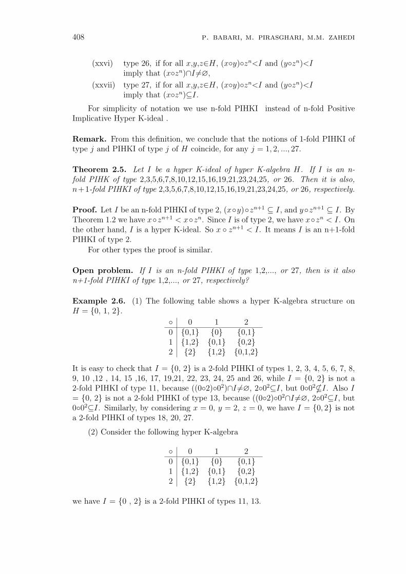
408 p. babari, m. pirasghari, m.m. zahedi
(xxvi) type 26, if for all x,y,z∈H, (xy)zn<I and (yzn)<Iimply that (xzn)∩I 6=∅,
(xxvii) type 27, if for all x,y,z∈H, (xy)zn<I and (yzn)<Iimply that (xzn)⊆I.
For simplicity of notation we use n-fold PIHKI instead of n-fold PositiveImplicative Hyper K-ideal .
Remark. From this definition, we conclude that the notions of 1-fold PIHKI oftype j and PIHKI of type j of H coincide, for any j = 1, 2, ..., 27.
Theorem 2.5. Let I be a hyper K-ideal of hyper K-algebra H. If I is an n-fold PIHK of type 2,3,5,6,7,8,10,12,15,16,19,21,23,24,25, or 26. Then it is also,n+1-fold PIHKI of type 2,3,5,6,7,8,10,12,15,16,19,21,23,24,25, or 26, respectively.
Proof. Let I be an n-fold PIHKI of type 2, (xy)zn+1 ⊆ I, and yzn+1 ⊆ I. ByTheorem 1.2 we have xzn+1 < xzn. Since I is of type 2, we have xzn < I. Onthe other hand, I is a hyper K-ideal. So x zn+1 < I. It means I is an n+1-foldPIHKI of type 2.
For other types the proof is similar.
Open problem. If I is an n-fold PIHKI of type 1,2,..., or 27, then is it alson+1-fold PIHKI of type 1,2,..., or 27, respectively?
Example 2.6. (1) The following table shows a hyper K-algebra structure onH = 0, 1, 2.
0 1 20 0,1 0 0,11 1,2 0,1 0,22 2 1,2 0,1,2
It is easy to check that I = 0, 2 is a 2-fold PIHKI of types 1, 2, 3, 4, 5, 6, 7, 8,9, 10 ,12 , 14, 15 ,16, 17, 19,21, 22, 23, 24, 25 and 26, while I = 0, 2 is not a2-fold PIHKI of type 11, because ((02)02)∩I 6=∅, 202⊆I, but 002*I. Also I= 0, 2 is not a 2-fold PIHKI of type 13, because ((02)02∩I 6=∅, 202⊆I, but002⊆I. Similarly, by considering x = 0, y = 2, z = 0, we have I = 0, 2 is nota 2-fold PIHKI of types 18, 20, 27.
(2) Consider the following hyper K-algebra
0 1 20 0,1 0 0,11 1,2 0,1 0,22 2 1,2 0,1,2
we have I = 0 , 2 is a 2-fold PIHKI of types 11, 13.
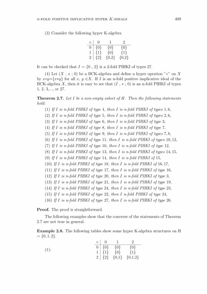
n-fold positive implicative hyper K-ideals 409
(3) Consider the following hyper K-algebra
0 1 20 0 0 01 1 0 12 2 0,2 0,2
It can be checked that I = 0 , 2 is a 2-fold PIHKI of types 27.
(4) Let (X , ∗ ; 0) be a BCK-algebra and define a hyper opration ”” on Xby xy=x∗y for all x, y ∈X. If I is an n-fold positive implicative ideal of theBCK-algebra X, then it is easy to see that (I , ∗ ; 0) is an n-fold PIHKI of types1, 2, 3,..., or 27.
Theorem 2.7. Let I be a non-empty subset of H. Then the following statementshold:
(1) If I is n-fold PIHKI of type 4, then I is n-fold PIHKI of types 1, 6,
(2) If I is n-fold PIHKI of type 5, then I is n-fold PIHKI of types 2, 6,
(3) If I is n-fold PIHKI of type 6, then I is n-fold PIHKI of type 3,
(4) If I is n-fold PIHKI of type 8, then I is n-fold PIHKI of type 7,
(5) If I is n-fold PIHKI of type 9, then I is n-fold PIHKI of types 7, 8,
(6) If I is n-fold PIHKI of type 11, then I is n-fold PIHKI of types 10, 12,
(7) If I is n-fold PIHKI of type 10, then I is n-fold PIHKI of type 12,
(8) If I is n-fold PIHKI of type 13, then I is n-fold PIHKI of types 14, 15,
(9) If I is n-fold PIHKI of type 14, then I is n-fold PIHKI of 15,
(10) If I is n-fold PIHKI of type 18, then I is n-fold PIHKI of 16, 17,
(11) If I is n-fold PIHKI of type 17, then I is n-fold PIHKI of type 16,
(12) If I is n-fold PIHKI of type 20, then I is n-fold PIHKI of type 3,
(13) If I is n-fold PIHKI of type 21, then I is n-fold PIHKI of type 19,
(14) If I is n-fold PIHKI of type 24, then I is n-fold PIHKI of type 23,
(15) If I is n-fold PIHKI of type 22, then I n-fold PIHKI of type 24,
(16) If I is n-fold PIHKI of type 27, then I is n-fold PIHKI of type 26.
Proof. The proof is straightforward.
The following examples show that the converse of the statements of Theorem2.7 are not true in general.
Example 2.8. The following tables show some hyper K-algebra structures on H= 0, 1, 2.
(1):
0 1 20 0 0 01 1 0 12 2 0,1 0,1,2
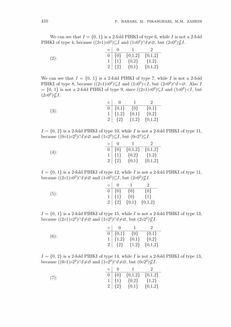
410 p. babari, m. pirasghari, m.m. zahedi
We can see that I = 0, 1 is a 2-fold PIHKI of type 6, while I is not a 2-foldPIHKI of type 4, because ((21)02)⊆I and (102)∩I 6=∅, but (202)*I.
(2):
0 1 20 0 0,1,2 0,1,21 1 0,2 1,22 2 0,1 0,1,2
We can see that I = 0, 1 is a 2-fold PIHKI of type 7, while I is not a 2-foldPIHKI of type 8, because ((21)02)⊆I and (102)<I, but (202)∩I=∅. Also I= 0, 1 is not a 2-fold PIHKI of type 9, since ((21)02)⊆I and (102)<I, but(202)*I.
(3):
0 1 20 0,1 0 0,11 1,2 0,1 0,22 2 1,2 0,1,2
I = 0, 2 is a 2-fold PIHKI of type 10, while I is not a 2-fold PIHKI of type 11,because ((01)22)∩I 6=∅ and (122)⊆I, but (022)⊆I.
(4):
0 1 20 0 0,1,2 0,1,21 1 0,2 1,22 2 0,1 0,1,2
I = 0, 1 is a 2-fold PIHKI of type 12, while I is not a 2-fold PIHKI of type 11,because ((21)02)∩I 6=∅ and (102)⊆I, but (202)*I.
(5):
0 1 20 0 0 01 1 0 12 2 0,1 0,1,2
I = 0, 1 is a 2-fold PIHKI of type 15, while I is not a 2-fold PIHKI of type 13,because ((21)22)∩I 6=∅ and (122)∩I 6=∅, but (222)*I.
(6):
0 1 20 0,1 0 0,11 1,2 0,1 0,22 2 1,2 0,1,2
I = 0, 2 is a 2-fold PIHKI of type 14, while I is not a 2-fold PIHKI of type 13,because ((01)22)∩I 6=∅ and (122)∩I 6=∅, but (022)*I.
(7):
0 1 20 0 0,1,2 0,1,21 1 0,2 1,22 2 0,1 0,1,2

n-fold positive implicative hyper K-ideals 411
I = 0, 2 is a 2-fold PIHKI of type 15, while I is not a 2-fold PIHKI of type 14,because
((12)02)∩I 6=∅ and (202)∩I 6=∅, but (102)∩I=∅.
(8):
0 1 20 0 0 01 1 0 12 2 0,2 0,2
I = 0, 1 is a 2-fold PIHKI of type 16, while I is not a 2-fold PIHKI of type 18,because ((21)22)∩I 6=∅ and (122)∩I 6=∅, but (222)*I.
(9):
0 1 20 0,1 0 0,11 1,2 0,1 0,22 2 1,2 0,1,2
We see that I = 0, 2 is a 2-fold PIHKI of type 17, while I is not a 2-fold PIHKIof type 18, because ((01)22)∩I 6=∅ and (122)<I, but (022)*I.
(10):
0 1 20 0 0,1,2 0,1,21 1 0,2 1,22 2 0,1 0,1,2
I = 0, 1 is a 2-fold PIHKI of type 16, while I is not a 2-fold PIHKI of type 17,because ((21)02)∩I 6=∅ and (102)<I, but (202)∩I=∅.
Also we see that I = 0, 1 is a 2-fold PIHKI of type 19, while I is not a2-fold PIHKI of type 20, becaus ((21)22)∩I 6=∅ and (122)∩I=∅, but (222)*I.
(11):
0 1 20 0,1 0 0,11 1,2 0,1 0,22 2 1,2 0,1,2
I = 0, 2 is a 2-fold PIHKI of type 24, while I is not a 2-fold PIHKI of type 22,because ((12)02)<I and (202)⊆I, but (102)*I.
(12):
0 1 20 0 0,1,2 0,1,21 1 0,2 1,22 2 0,1 0,1,2
We see that I = 0, 1 is a 2-fold PIHKI of type 25, but I is not a 2-fold PIHKIof type 26, because ((21)02)<I and (102)<I, (202)∩I=∅.

412 p. babari, m. pirasghari, m.m. zahedi
(13):
0 1 20 0,1 0 0,11 1,2 0,1 0,22 2 1,2 0,1,2
I = 0, 2 is a 2-fold PIHKI of type 26, while I is not a 2-fold PIHKI of type 27,because ((01)22)<I and (122)<I, but (022)*I.
Also we see that I = 0, 1 is a 2-fold PIHKI of types 2 and 3, while I is nota 2-fold PIHKI of type 1, because ((21)02)⊆I and (102)⊆I, but (202)*I.
Theorem 2.9. Let I be a hyper K-algebra of H. Then the following statementare equivalent:
(1) xyn<I,
(2) (xyn)∩I 6=∅.
Proof. (1)⇒(2) Assume xyn<I, then there exist a∈I, and t∈xyn such thatt<a. Thus 0∈ta. Now, since 0∈I and 0∈0a, then ta<I. So t∈I. Hence,(xyn)∩I 6=∅.
(2)⇒(1) It is obvious.
Theorem 2.10. Let I be a hyper K-ideal of a hyper K-algebra H. Then thefollowing statements are equivalent:
(1) I is an n-fold PIHKI of type 14,
(2) I is an n-fold PIHKI of type 15,
(3) I is an n-fold PIHKI of type 16,
(4) I is an n-fold PIHKI of type 17,
(5) I is an n-fold PIHKI of type 19,
(6) I is an n-fold PIHKI of type 21,
(7) I is an n-fold PIHKI of type 25,
(8) I is an n-fold PIHKI of type 26.
Proof. (1)⇒(2) Let I be an n-fold PIHKI of type 14. So for all x,y,z ∈ H, if((xy)zn)∩I 6=Ø, and (yzn)∩I 6=Ø, then (xzn)∩I 6=Ø. On the other hand, byTheorem 2.9 we have (xzn)<I. Thus I is of type 15.
(8)⇒(1) Let I be an n-fold PIHKI of type 26. So for all x,y,z ∈ H, if((xy)zn)<I, and yzn<I, then (xzn)∩I 6=Ø. Now, by Theorem 2.9 we have((xy)zn)∩I 6=Ø, and so, (yzn)∩I 6=Ø implies that (xzn)∩I 6=Ø. Thus I is oftype 14.
The proof of other statements can be obtained by the same way.
Theorem 2.11. Let I be a hyper K-ideal of a hyper K-algebra H. Then thefollowing statements are equivalent:
(1) I is an n-fold PIHKI of type 13,
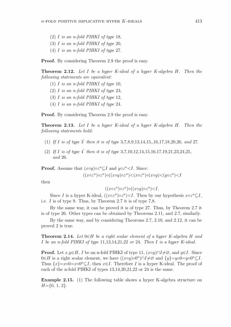
n-fold positive implicative hyper K-ideals 413
(2) I is an n-fold PIHKI of type 18,
(3) I is an n-fold PIHKI of type 20,
(4) I is an n-fold PIHKI of type 27.
Proof. By considering Theorem 2.9 the proof is easy.
Theorem 2.12. Let I be a hyper K-ideal of a hyper K-algebra H. Then thefollowing statements are equivalent:
(1) I is an n-fold PIHKI of type 10,
(2) I is an n-fold PIHKI of type 23,
(3) I is an n-fold PIHKI of type 12,
(4) I is an n-fold PIHKI of type 24.
Proof. By considering Theorem 2.9 the proof is easy.
Theorem 2.13. Let I be a hyper K-ideal of a hyper K-algebra H. Then thefollowing statements hold:
(1) If I is of type 3′then it is of type 3,7,8,9,13,14,15,,16,17,18,20,26, and 27.
(2) If I is of type 4′then it is of type 3,7,10,12,14,15,16,17,19,21,23,24,25,
and 26.
Proof. Assume that (xy)zn⊆I and yzn<I. Since:
((xzn)zn)((xy)zn)<(xzn)(xy)<(yzn)<I
then
((xzn)zn)((xy)zn)<I.
Since I is a hyper K-ideal, ((xzn)zn)<I. Then by our hypothesis xzn⊆I,i.e. I is of type 9. Thus, by Theorem 2.7 it is of type 7,8.
By the same way, it can be proved it is of type 27. Thus, by Theorem 2.7 itis of type 26. Other types can be obtained by Theorems 2.11, and 2.7, similarly.
By the same way, and by considering Theorems 2.7, 2.10, and 2.12, it can beproved 2 is true.
Theorem 2.14. Let 0∈H be a right scalar element of a hyper K-algebra H andI be an n-fold PIHKI of type 11,13,14,21,22 or 24. Then I is a hyper K-ideal.
Proof. Let x,y∈H, I be an n-fold PIHKI of type 11, (xy)∩I 6=∅, and y∈I. Since0∈H is a right scalar element, we have ((xy)0n)∩I 6=∅ and y=y0=y0n⊆I.Thus x=x0=x0n⊆I, then x∈I. Therefore I is a hyper K-ideal. The proof ofeach of the n-fold PIHKI of types 13,14,20,21,22 or 24 is the same.
Example 2.15. (1) The following table shows a hyper K-algebra structure onH=0, 1, 2.

414 p. babari, m. pirasghari, m.m. zahedi
0 1 20 0,1 0,1,2 0,1,21 1 0,1 1,22 1,2 0,1,2 0,1,2
Then I = 0 , 1 is an n-fold PIHKI of type 21, for any n∈N , while I is nota hyper K-ideal, because (21)∩I 6=∅, and 1∈I, but 2 /∈ I. Also we see that 0∈His not a right scalar element.
(2) Consider the following hyper K-algebra
0 1 20 0,1 0 0,11 1,2 0,1 0,22 2 1,2 0,1,2
We see that 0∈H is not a right scalar element and I = 0 , 2 is an n-foldPIHKI of types 11, 14, 22, and 24, for any n∈N , while I is not a hyper K-ideal,because (12)∩I 6=∅, and 2∈I, but 1 /∈ I. I = 0 , 1 is an n-fold PIHKI of type13, for any n∈N , while I is not a hyper K-ideal, because (21)∩I 6=∅, and 1∈I,but 2 /∈ I.
Note that Example 2.15 shows the condition 0∈H is a right scalar is necessaryin Theorem 2.14.
Theorem 2.16. Let 0∈H be a right scalar element of a hyper K-algebra H andI be closed. If I is an n-fold PIHKI of type 12, 15, 16, 19 or 23, then I is a weakhyper K-ideal.
Proof. Let I be an n-fold PIHKI of type 12, x,y∈H, (xy)⊆I and y∈I. Since 0∈His a right scalar element, ((xy)0n)∩I 6=∅ and (y0)⊆I imply that (x0n) < I. Sothere exists i∈I such that x0n < i. Therefore (x0n−1)i<0. Thus, there existsk∈(x0n−1)i such that k<0. Hence, by 0<k we have k=0, i.e. 0∈(x0n−1)i. Itmeans x0n−1<i. Repeatedly using this way it follows x<i. Now since I is closed,we obtain that x∈I. Therefore I is a weak hyper K-ideal. The proof of each ofthe n-fold PIHKI of types 15, 16, 19, or 23 is the same.
Theorem 2.17. Let 0∈H be a right scalar element of a hyper K-algebra H andI be an n-fold PIHKI of type 18, 20, 26 or 27. Then I is a weak hyper K-ideal.
Proof. The proof is similar to the proof of Theorem 2.16.
Example 2.18. Consider the following hyper K-algebra
0 1 20 0,1 0 0,11 1,2 0,1 0,22 2 1,2 0,1,2
n-fold positive implicative hyper K-ideals 415
In this example I = 0 , 2 is an n-fold PIHKI of types 12, 15, 16, 19, and 23,for any n∈N , while I is not a hyper K-ideal, because we see that I is not closedand 0∈H is not a right scalar.
Definition 2.19. Let H be a hyper K-algebra and I⊆H and a∈I. We defineIan = x∈H | (xan)∩I 6=∅ .
Theorem 2.20. Let H be a hyper K-algebra. Then I is an n-fold PIHKI of type14 if and only if for all a∈H, Ian is a hyper K-ideal.
Proof. Let for all x,y,a∈H, ((xy)∩Ian) 6= ∅, y∈Ian . Then ((xy)an)∩I 6= ∅,(yan)∩I 6= ∅. Since I is an n-fold PIHKI of type 14, (xan)∩I 6= ∅. Thereforex∈Ian , i.e. I is a hyper K-ideal.
Conversely, let for all x,y,a∈H, ((xy)an)∩I 6= ∅ and (yan)∩I 6= ∅. Then,xy⊆ Ian . So,by Theorem 2.9 xy< Ian . Now, since y∈Ian and Ian is a hyperK-ideal, we obtain x∈Ian . Thus, (xan)∩I 6= ∅, i.e. I is an n-fold PIHKI oftype 14.
3. n-fold positive implicative hyper K-ideals in simple hyper K-algebras
In this part (H, , 0) is a simple hyper K-algebra, unless otherwise is stated.
Theorem 3.1. Let 0 ∈ I ⊆ H. Then
(i) I is an n-fold PIHKI of type 2 if and only if I is an n-fold PIHKIof type 3,
(ii) I is an n-fold PIHKI of type 4 if and only if I is an n-fold PIHKIof type 9,
(iii) I is an n-fold PIHKI of type 5 if and only if I is an n-fold PIHKIof type 6(7,8),
(iv) I is an n-fold PIHKI of type 11 if and only if I is an n-fold PIHKIof type 22,
(v) I is an n-fold PIHKI of type 10 if and only if I is an n-fold PIHKIof type 12(23,24),
(vi) I is an n-fold PIHKI of type 13 if and only if I is an n-fold PIHKIof type 18(20,27),
(vii) I is an n-fold PIHKI of type 14 if and only if I is an n-fold PIHKIof type 15(16,17,19,21,25,26).
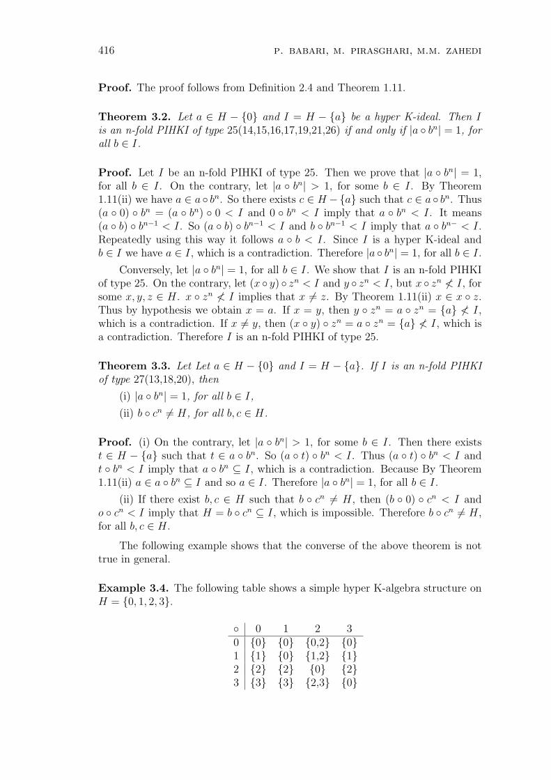
416 p. babari, m. pirasghari, m.m. zahedi
Proof. The proof follows from Definition 2.4 and Theorem 1.11.
Theorem 3.2. Let a ∈ H − 0 and I = H − a be a hyper K-ideal. Then Iis an n-fold PIHKI of type 25(14,15,16,17,19,21,26) if and only if |a bn| = 1, forall b ∈ I.
Proof. Let I be an n-fold PIHKI of type 25. Then we prove that |a bn| = 1,for all b ∈ I. On the contrary, let |a bn| > 1, for some b ∈ I. By Theorem1.11(ii) we have a ∈ a bn. So there exists c ∈ H −a such that c ∈ a bn. Thus(a 0) bn = (a bn) 0 < I and 0 bn < I imply that a bn < I. It means(a b) bn−1 < I. So (a b) bn−1 < I and b bn−1 < I imply that a bn− < I.Repeatedly using this way it follows a b < I. Since I is a hyper K-ideal andb ∈ I we have a ∈ I, which is a contradiction. Therefore |a bn| = 1, for all b ∈ I.
Conversely, let |a bn| = 1, for all b ∈ I. We show that I is an n-fold PIHKIof type 25. On the contrary, let (x y) zn < I and y zn < I, but x zn ≮ I, forsome x, y, z ∈ H. x zn ≮ I implies that x 6= z. By Theorem 1.11(ii) x ∈ x z.Thus by hypothesis we obtain x = a. If x = y, then y zn = a zn = a ≮ I,which is a contradiction. If x 6= y, then (x y) zn = a zn = a ≮ I, which isa contradiction. Therefore I is an n-fold PIHKI of type 25.
Theorem 3.3. Let Let a ∈ H − 0 and I = H − a. If I is an n-fold PIHKIof type 27(13,18,20), then
(i) |a bn| = 1, for all b ∈ I,
(ii) b cn 6= H, for all b, c ∈ H.
Proof. (i) On the contrary, let |a bn| > 1, for some b ∈ I. Then there existst ∈ H − a such that t ∈ a bn. So (a t) bn < I. Thus (a t) bn < I andt bn < I imply that a bn ⊆ I, which is a contradiction. Because By Theorem1.11(ii) a ∈ a bn ⊆ I and so a ∈ I. Therefore |a bn| = 1, for all b ∈ I.
(ii) If there exist b, c ∈ H such that b cn 6= H, then (b 0) cn < I ando cn < I imply that H = b cn ⊆ I, which is impossible. Therefore b cn 6= H,for all b, c ∈ H.
The following example shows that the converse of the above theorem is nottrue in general.
Example 3.4. The following table shows a simple hyper K-algebra structure onH = 0, 1, 2, 3.
0 1 2 30 0 0 0,2 01 1 0 1,2 12 2 2 0 23 3 3 2,3 0
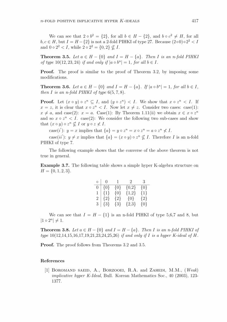
n-fold positive implicative hyper K-ideals 417
We can see that 2 b2 = 2, for all b ∈ H − 2, and b c2 6= H, for allb, c ∈ H, but I = H−2 is not a 2-fold PIHKI of type 27. Because (20)22 < Iand 0 22 < I, while 2 22 = 0, 2 * I.
Theorem 3.5. Let a ∈ H − 0 and I = H − a. Then I is an n-fold PIHKIof type 10(12, 23, 24) if and only if |a bn| = 1, for all b ∈ I.
Proof. The proof is similar to the proof of Theorem 3.2, by imposing somemodifications.
Theorem 3.6. Let a ∈ H − 0 and I = H − a. If |a bn| = 1, for all b ∈ I,then I is an n-fold PIHKI of type 6(5, 7, 8).
Proof. Let (x y) zn ⊆ I, and (y zn) < I. We show that x zn < I. Ifx = z, it is clear that x zn < I. Now let x 6= z. Consider two cases: case(1):x 6= a, and case(2): x = a. Case(1): By Theorem 1.11(ii) we obtain x ∈ x zn
and so x zn < I. case(2): We consider the following two sub-cases and showthat (x y) zn * I or y z ≮ I.
case(i′): y = x implies that a = y zn = x zn = a zn ≮ I.
case(ii′): y 6= x implies that a = (x y) zn * I. Therefore I is an n-fold
PIHKI of type 7.
The following example shows that the converse of the above theorem is nottrue in general.
Example 3.7. The following table shows a simple hyper K-algebra structure onH = 0, 1, 2, 3.
0 1 2 30 0 0 0,2 01 1 0 1,2 12 2 2 0 23 3 3 2,3 0
We can see that I = H − 1 is an n-fold PIHKI of type 5,6,7 and 8, but|1 2n| 6= 1.
Theorem 3.8. Let a ∈ H −0 and I = H −a. Then I is an n-fold PIHKI oftype 10(12,14,15,16,17,19,21,23,24,25,26) if and only if I is a hyper K-ideal of H.
Proof. The proof follows from Theorems 3.2 and 3.5.
References
[1] Boromand saeid, A., Borzooei, R.A. and Zahedi, M.M., (Weak)implicative hyper K-Ideal, Bull. Korean Mathematics Soc., 40 (2003), 123-1377.
418 p. babari, m. pirasghari, m.m. zahedi
[2] Borzooei, R.A., Hyper BCK and K-algebras, Ph.D. Thesis, Shahid Ba-honar University of Kerman, Dept. of Mathematics, 2000.
[3] Borzooei, R.A., Corsini, P. and Zahedi, M.M., Some kinds of positiveimplicative hyper K-ideals, J. Discrete Mathematics and Cryptography, 6(2003), 97-108.
[4] Borzooei, R.A., Hasankhani, A., Zahedi, M.M. and B. Jun, Y.B.,On hyper K-algebras, Scientiae Mathematicae Japonicae, vol. 52, no. 1(2000), 113-121.
[5] Borzooei, R.A. and Zahedi, M.M., Positive implicative hyper K-ideals,Scientiae Mathematicae Japonicae, vol. 53, no. 3 (2001), 525-533.
[6] Harizavi,H., Hyper BCK-algebra and Related Structures, Ph.D. Thesis,Sistan and Balochestan University, Dept. of Mathematics, 2006.
[7] Iseki, K. and Tanaka, S., An introduction to the theory of BCK-algebras,Scientiae Mathematicae Japonicae, 23 (1978), 1-26.
[8] Jun, Y.B., Zahedi, M.M., Xin, X.L. and Borzooei, R., On hyperBCK-algebras, Italian J. Pure and Appl. Math., no. 11 (2000), 127-136.
[9] Jun, Y.B. and Xin, X.L., Positive implicative hyper BCK -algebras, Sci-entiae Mathematicae Japonicae, 55 (3)(2002), 97-106.
[10] Marty, F., Sur une generalization de la notion de groups, 8th congressMath. Scandinaves, Stockholm, 1934, 45-49.
[11] Meng, J., Jun, Y.B., BCK-algebra, Kyung Moonsa, Seoul, 1994.
[12] Roodbari, T., Positive implicative and commutative hyper k-idaels, Ph.D.Thesis, Islamic Azad University of Kerman Branch, Dept. of Mathematics,Kerman, Iran, 2008.
[13] Roodbari, T. and Zahedi, M.M., Positive implicative hyper K-ideals II,Scientiae Mathematicae Japonicae, 66, no. 3 (2007), 391-404: e2007, 507-520.
[14] Torkzadeh, L., Zahedi, M.M., Commutative hyper K-ideals and Quasi-commutative hyper K-algebras, Italian Journal Of Pure and Applied Mathe-matics, to appear.
[15] Yisheng, H., CI-Algebra, Science Press, Beijing, China, 2006.
Accepted: 12.03.2012
ITALIAN JOURNAL OF PURE AND APPLIED MATHEMATICS
INFORMATION FOR AUTHORS
• Before an article can be published in the Italian Journal of Pure and Applied Mathematics, the author is required to contribute with a small fee, which has to be calculated with the following formula:
fee = EUR (20 + 3n)
where n is the number of pages of the article to be published.
• The above amount has to be payed through an international credit transfer in the folowing bank account:
Bank name: CASSA DI RISPARMIO DEL FRIULI VENEZIA GIULIAIBAN code: IT 98 V 06340 12300 07404361962TBIC code: IBSPIT2Account owner: FORUM EDITRICE UNIVERSITARIA UDINESE SRL
VIA LARGA 3833100 UDINE (ITALY)
• All bank commissions must be payed by the author, adding them to the previous calculated net amount
• Include the following mandatory causal in the credit transfer transaction:
CONTRIBUTO PUBBLICAZIONE ARTICOLO SULL’ITALIAN JOURNAL OF PURE AND APPLIED MATHEMATICS
• After the transaction ends successfully, the author is requested to send an e-mail to the following address: [email protected]. This e-mail should contain the author's personal information (Last name, First Name, Postemail Address, City and State), in order to allow Forum Editrice to create an invoice for the author himself.
• Payments, orders or generic fees will not be accepted if they refer to Research Institutes, Universities or any other public and private orgtanizations).
• Finally, when the payment has been done and the e-mail has been received, Forum Editrice will issue an invoice receipt in PDF format and will send it by e-mail to the author.
IJPAM – Italian Journal of Pure and Applied MathematicsIssue n° 29-2012
PublisherForum Editrice Universitaria Udinese Srl
Via Palladio 8 - 33100 UdineTel: +39-0432-26001, Fax: +39-0432-296756
This journal is published with the financial support of: 1 - Hatef University, Zahedan, Iran
2 - Authors of the papers of the single number
Rivista semestrale: Autorizzazione Tribunale di Udine n. 8/98 del 19.3.98 - Direttore responsabile: Piergiulio Corsini
ISSN 2239-0227