General rights Copyright and moral rights for the publications made accessible in the public portal are retained by the authors and/or other copyright owners and it is a condition of accessing publications that users recognise and abide by the legal requirements associated with these rights.

Users may download and print one copy of any publication from the public portal for the purpose of private study or research.

You may not further distribute the material or use it for any profit-making activity or commercial gain

You may freely distribute the URL identifying the publication in the public portal If you believe that this document breaches copyright please contact us providing details, and we will remove access to the work immediately and investigate your claim.

Downloaded from orbit.dtu.dk on: Apr 23, 2020

Iso-geometric shape optimization of magnetic density separators

Dang Manh, Nguyen; Evgrafov, Anton ; Gravesen, Jens; Lahaye, Domenico

Published in:Compel

Link to article, DOI:10.1108/COMPEL-07-2013-0234

Publication date:2014

Document VersionPeer reviewed version

Link back to DTU Orbit

Citation (APA):Dang Manh, N., Evgrafov, A., Gravesen, J., & Lahaye, D. (2014). Iso-geometric shape optimization of magneticdensity separators. Compel, 33(4), 1416-1433. https://doi.org/10.1108/COMPEL-07-2013-0234

Iso-Geometric Shape Optimization

of Magnetic Density Separators

June 5, 2014

AbstractPurpose - The waste recycling industry increasingly relies on magneticdensity separators. These devices generate an upward magnetic force inferro-fluids allowing to separate the immersed particles according to theirmass density. Recently, a new separator design has been proposed thatsignificantly reduces the required amount of permanent magnet material.The purpose of this paper is to reduce the undesired end-effects in theupward force that this design generates by altering the shape of the fer-romagnetic covers of the individual poles.Design/methodology/approach - We represent the shape of the fer-romagnetic pole covers with B-splines and define a cost functional thatmeasures the non-uniformity in the magnetic force in an area above thepoles. We apply an isogeometric shape optimization procedure, which al-lows us to accurately represent, analyze and optimize the geometry usingonly a few design variables. The design problem is regularized by imposingconstraints that enforce the convexity of the pole cover shapes. It is solvedby a non-linear optimization procedure. We validate the implementationof our algorithm using a simplified variant of our design problem with aknown analytical solution. The algorithm is subsequently applied to theproblem posed.Research limitations/implications - The shape optimization attainsits target and yields pole cover shapes that give rise to a magnetic fieldthat is uniform over a larger domain. This increased uniformity is obtainedat the cost of a pole cover shape that differs per pole. This limitation hasnegligible impact on the manufacturing of the separator. The new polecover shapes, therefore, lead to improved performance of the density sep-aration.Originality/value - This paper treats the shapes optimization of mag-netic density separators systematically and presents new shapes for theferromagnetic pole covers. Due to the larger uniformity of the generatedfield, these shapes should enable larger amounts of waste to be processedthan the previous design.Keywords - Magnetic density separation, shape optimization, iso-geometricanalysis.Paper type - Research paper

1 Introduction

Magnetic density separators are increasingly being used by the waste recyclingindustry. The development and usage of these devices is extensively described in

1

the monograph [Svoboda (2004)]. The separators considered here exert an up-ward magnetic force on waste particles immersed in a container with ferro-fluid.As the magnitude of the resultant of the hydrostatic and magnetic buoyancyforce is proportional to the mass density of the waste particles, these particleswill float at mass density specific heights. If this height is constant across lat-eral directions in the container, particles of the same mass density can easily beremoved from the container.

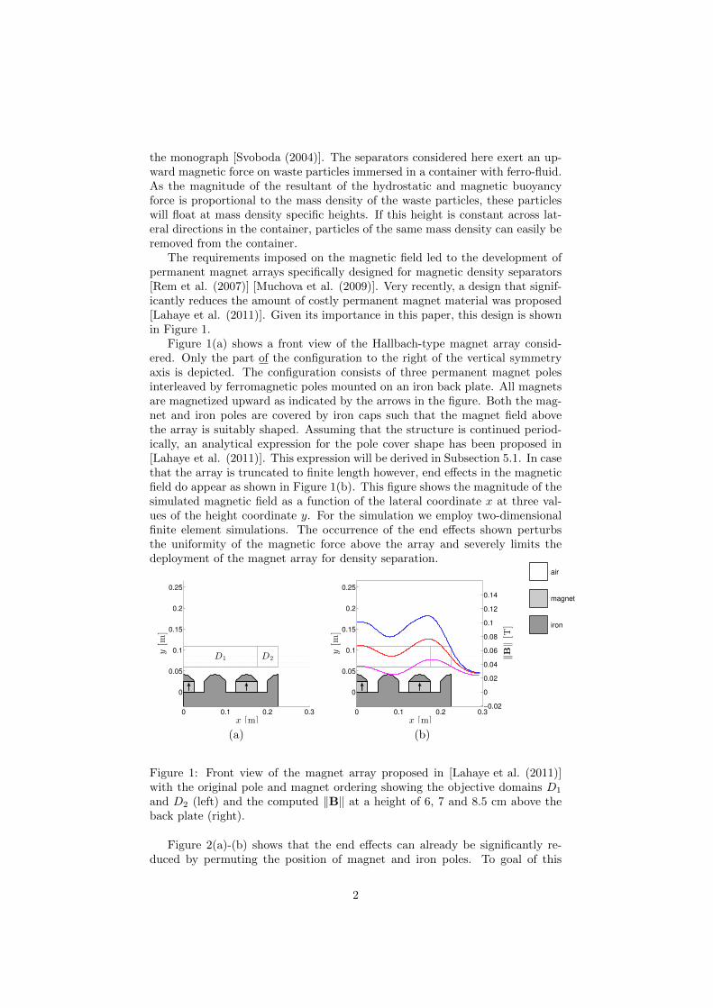
The requirements imposed on the magnetic field led to the development ofpermanent magnet arrays specifically designed for magnetic density separators[Rem et al. (2007)] [Muchova et al. (2009)]. Very recently, a design that signif-icantly reduces the amount of costly permanent magnet material was proposed[Lahaye et al. (2011)]. Given its importance in this paper, this design is shownin Figure 1.

Figure 1(a) shows a front view of the Hallbach-type magnet array consid-ered. Only the part of the configuration to the right of the vertical symmetryaxis is depicted. The configuration consists of three permanent magnet polesinterleaved by ferromagnetic poles mounted on an iron back plate. All magnetsare magnetized upward as indicated by the arrows in the figure. Both the mag-net and iron poles are covered by iron caps such that the magnet field abovethe array is suitably shaped. Assuming that the structure is continued period-ically, an analytical expression for the pole cover shape has been proposed in[Lahaye et al. (2011)]. This expression will be derived in Subsection 5.1. In casethat the array is truncated to finite length however, end effects in the magneticfield do appear as shown in Figure 1(b). This figure shows the magnitude of thesimulated magnetic field as a function of the lateral coordinate x at three val-ues of the height coordinate y. For the simulation we employ two-dimensionalfinite element simulations. The occurrence of the end effects shown perturbsthe uniformity of the magnetic force above the array and severely limits thedeployment of the magnet array for density separation.

0 0.1 0.2 0.3

0

0.05

0.1

0.15

0.2

0.25

D1 D2

x [m]

y[m

]

0 0.1 0.2 0.3

0

0.05

0.1

0.15

0.2

0.25

x [m]

y[m

]

−0.02

0

0.02

0.04

0.06

0.08

0.1

0.12

0.14

‖B‖[T

]

0 1 2 3 4 50

1

2

3

4

5

6

iron

magnet

air

(a) (b)

Figure 1: Front view of the magnet array proposed in [Lahaye et al. (2011)]with the original pole and magnet ordering showing the objective domains D1

and D2 (left) and the computed ‖B‖ at a height of 6, 7 and 8.5 cm above theback plate (right).

Figure 2(a)-(b) shows that the end effects can already be significantly re-duced by permuting the position of magnet and iron poles. To goal of this

2

0 0.2 0.4 0.6 0.8 10

0.2

0.4

0.6

0.8

1

‖B‖(x, 0.06) [T]‖B‖(x, 0.07) [T]‖B‖(x, 0.085) [T]

0 0.2 0.4 0.6 0.8 10

0.2

0.4

0.6

0.8

1

−0.05 ∂∂y‖B‖(x, 0.06) [T/m]

−0.05 ∂∂y‖B‖(x, 0.07) [T/m]

−0.05 ∂∂y‖B‖(x, 0.085) [T/m]

0 0.1 0.2 0.3

0

0.05

0.1

0.15

0.2

0.25

x [m]

y[m

]

−0.02

0

0.02

0.04

0.06

0.08

0.1

0.12

0.14

‖B‖[T

]

0 0.1 0.2 0.3

0

0.05

0.1

0.15

0.2

0.25

x [m]

y[m

]

0

1

2

3

4

5

6

7

−0.05∂‖B‖

∂y

[T/m]

(a) (b)

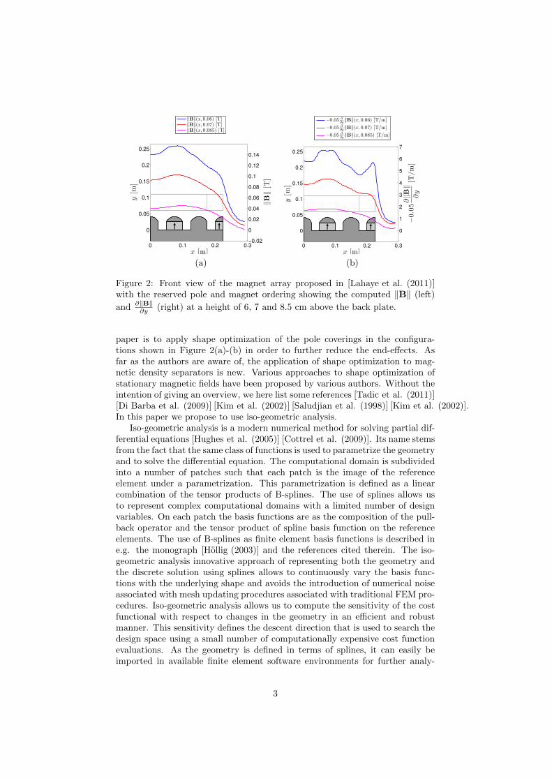
Figure 2: Front view of the magnet array proposed in [Lahaye et al. (2011)]with the reserved pole and magnet ordering showing the computed ‖B‖ (left)

and ∂‖B‖∂y (right) at a height of 6, 7 and 8.5 cm above the back plate.

paper is to apply shape optimization of the pole coverings in the configura-tions shown in Figure 2(a)-(b) in order to further reduce the end-effects. Asfar as the authors are aware of, the application of shape optimization to mag-netic density separators is new. Various approaches to shape optimization ofstationary magnetic fields have been proposed by various authors. Without theintention of giving an overview, we here list some references [Tadic et al. (2011)][Di Barba et al. (2009)] [Kim et al. (2002)] [Saludjian et al. (1998)] [Kim et al. (2002)].In this paper we propose to use iso-geometric analysis.

Iso-geometric analysis is a modern numerical method for solving partial dif-ferential equations [Hughes et al. (2005)] [Cottrel et al. (2009)]. Its name stemsfrom the fact that the same class of functions is used to parametrize the geometryand to solve the differential equation. The computational domain is subdividedinto a number of patches such that each patch is the image of the referenceelement under a parametrization. This parametrization is defined as a linearcombination of the tensor products of B-splines. The use of splines allows usto represent complex computational domains with a limited number of designvariables. On each patch the basis functions are as the composition of the pull-back operator and the tensor product of spline basis function on the referenceelements. The use of B-splines as finite element basis functions is described ine.g. the monograph [Hollig (2003)] and the references cited therein. The iso-geometric analysis innovative approach of representing both the geometry andthe discrete solution using splines allows to continuously vary the basis func-tions with the underlying shape and avoids the introduction of numerical noiseassociated with mesh updating procedures associated with traditional FEM pro-cedures. Iso-geometric analysis allows us to compute the sensitivity of the costfunctional with respect to changes in the geometry in an efficient and robustmanner. This sensitivity defines the descent direction that is used to search thedesign space using a small number of computationally expensive cost functionevaluations. As the geometry is defined in terms of splines, it can easily beimported in available finite element software environments for further analy-

3

sis. The advantages of isogeometric analysis for shape optimization are furtherelaborated in e.g. [Cho et al. (2009)] [Nguyen (2012)] [Nguyen et al. (2012)].

In this paper we apply iso-geometric shape optimization to the magneticdensity separators shown in Figure 2(a)-(b). Our goal is to shape the covers ofthe individual poles in such a way to minimize the non-uniformity of derivativeof the magnitude of the magnetic flux in lateral direction in an area abovethe poles. We introduce a functional that measures this non-uniformity andminimize this functional over two objective domains to investigate the influenceof end-effects. Our algorithm produces new shapes that significantly improvethe field uniformity and that therefore renders the device much more useful inindustrial applications.

This paper is structured as follows: in Section 2 we describe the shapeoptimization problem we set out to solve. In Section 3 we briefly review the iso-geometric analysis and shape optimization technique that we intend to employ.In Section 4 we give more details on the shape representation using B-splinesas it is an essential ingredient in the approach that we adopt. In Section 5 themethodology we advocate is tested on a design problem with a known analyticalsolution and on two versions of the shape optimization problem of the magneticdensity separator. In Section 6 finally conclusions are drawn.

2 Formulation of the Shape Optimization Prob-lem

In this section we formulate the shape optimization problem of the magnet arrayby giving details of the magnetic field equation, the cost functional, the designvariables and the regularization technique.

The objective of the shape optimization is to find shapes of the covers of themagnet and ferromagnetic poles that yield a magnetic force with a variation inthe lateral coordinate that is better suited for the density separation on wasteparticles immersed in the ferro-fluid in the container placed in the magnetic field.Waste particles in the magnetic field experience the downward gravitational pull,the upward hydrostatic buoyancy force and the upward magnetic force from theferro-fluid. If the latter is made independent of the lateral (x-) coordinate,the resultant force is laterally invariant as well, and waste particles with thesame mass density will float at an laterally invariant height. This facilitates theremoval of the different particles from the fluid and renders the device attractivefrom an industrial point of view. We stress here that unlike other approachesfor synthesizing the magnetic field that appeared in the literature, our objectiveis not to control individual field components, but rather the resulting magneticforce. Computing this force requires computing second order derivatives of themagnetic (either scalar or vector) potential in the post-processing stage of afield analysis.

A ferro-fluid with mass density ρf and saturation magnetization Mf willreact to being placed in a spatially varying magnetic field B(x, y) by a changein its density to its so-called apparent density ρapp. The latter is proportional tothe gradient of the magnitude magnetic field in the y-direction ∂‖B‖/∂y. More

4

precisely, we have that [Rosensweig (1987)] [Svoboda (2004)]

ρapp = ρf +Mf

g

∂‖B‖∂y

, (1)

where g is the gravitational constant. The computation of the magnetic forcerequires evaluating second order derivatives of the (scalar or vector) magneticpotential as is typically the case in magnetic force computation methods usingfor instance the virtual work on Maxwell stress tensor method. In a finiteelement analysis, these second order partial derivatives can be evaluated elementby element. To guarantee sufficient smoothness of the computed second orderderivatives we will use in this work second order approximations unless statedotherwise. A contour plot of ∂‖B‖/∂y generated by the design shown in Figure 1is given in [Nguyen (2012)]. The upward force by the ferro-fluid is proportionalits apparent density ρapp. The condition of the lateral invariance of the forceby the ferro-fluid can therefore be expressed as

∂2‖B‖∂x ∂y

= 0 . (2)

Our objective is therefore to enforce this condition, at least approximately, overa region located above the magnet array.

From here on we will only consider the magnet array given in [Lahaye et al. (2011)]with reserved magnet and pole ordering shown in Figure 2. Motivating thischoice is the fact that the magnets placed at the extremities allows a bettercontrol of the end effects. We will compute the magnetic field generated bythe magnet array using a vector potential formulation [Sylvester et al. (1996)].In two-dimensional perpendicular current configurations and in the presence ofvertically (y-) magnetized permanent magnets with remanent flux density Br =(0, Br, 0), the double curl equation for the vector potential A = (0, 0, Az(x, y))reduces to

− ∂

∂x

(1

µ

∂Az∂x

)− ∂

∂y

(1

µ

∂Az∂y

)=

1

µ

∂Br∂x

, (3)

where the relative magnetic permeability µr is set to 1000 and to 1 in the ironand permanent magnet domain, respectively. The ferro-fluid is diluted withwater to such an extend that its influence on the magnetic field is negligible. Theneodymium magnets in our simulations have a remanence of Br = 1.235 T. Thefield equation is supplied with appropriate insulating and symmetry boundaryconditions.

The evaluation of Condition (2), requires the computation of third orderderivatives of Az. To avoid this order of derivation to appear in the objectivefunction, we replace Condition (2) by the minimization of the dispersion D(y) of∂‖B‖/∂y in x-direction, i.e., we aim at reducing the difference between ∂‖B‖/∂yand its average value along horizontal lines in Ω0 = [x1, x2] × [y1, y2]. This

5

motivates the following definition of the cost functional

I0[Az; Ω0] =

∫ y2

y1

D(y) dy

=

∫ y2

y1

[∫ x2

x1

(∂‖B‖∂y

− 1

x2 − x1

∫ x2

x1

∂‖B‖∂y

dx

)2

dx

]dy

=

∫ y2

y1

[∫ x2

x1

(∂‖B‖∂y

)2

dx− 1

x2 − x1

(∫ x2

x1

∂‖B‖∂y

dx

)2]

dy .(4)

In this functional (with unit T 2) only derivatives of Az up to order two appear.Numerical experiments in Section 5, in which we will seek to minimize thequantity

I0(Az; Ω0) = log10[I0(Az; Ω0)/area(Ω0)] (5)

will give evidence that the cost functional is indeed appropriately chosen. Wewill perform the optimization using a gradient-based optimization algorithmthat requires the derivative of the cost functional with respect to design variablesthat define the geometry. The deployment of iso-geometric analysis method ismotivated by its ability to compute these derivatives without the inconveniencesassociated with more traditional finite element approaches.

We will conduct numerical studies for two choices for the objective domainΩ0. We define the subdomains D1 and D2 shown in Figure 1 by

D1 = [0, 0.175]× [0.06, 0.11] [m×m] ,

D2 = [0.175, 0.225]× [0.06, 0.11] [m×m] ,(6)

respectively. We set Ω0 equal to the domain D1 ∪D2 in the first study. In thesecond we restrict the objective domain to the interior by setting Ω0 = D1.

3 Isogeometric shape optimization

In this section we briefly describe the iso-geometric analysis (IGA) method forsolving the magnetic field equation (3) and for the shape optimization of themagnetic density separator shown in Figure 2(a)-(b). This section consists offour subsections. In the first we describe how the geometry is discretized usingB-splines in such a way that the designable boundaries can be represented usinga limited number of design variables. In the second subsection we cast the mag-netic field equation in a Galerkin variational form and discretize this formulationin space using basis functions defined in terms of the domain parametrization.This choice of the basis functions is the key idea of the IGA method. In thethird subsection we give the first order sensitivity equations for changes in thecoefficients of the discrete solutions with changes in the design parameters de-scribing the geometry. In the fourth subsection we regularize the shape optimiza-tion problem introduced. We refer to [Cottrel et al. (2009)] [Cho et al. (2009)][Hughes et al. (2005)] [Nguyen (2012)] [Nguyen et al. (2012)] for more detailson the material presented in this section.

6

3.1 Geometry Discretization

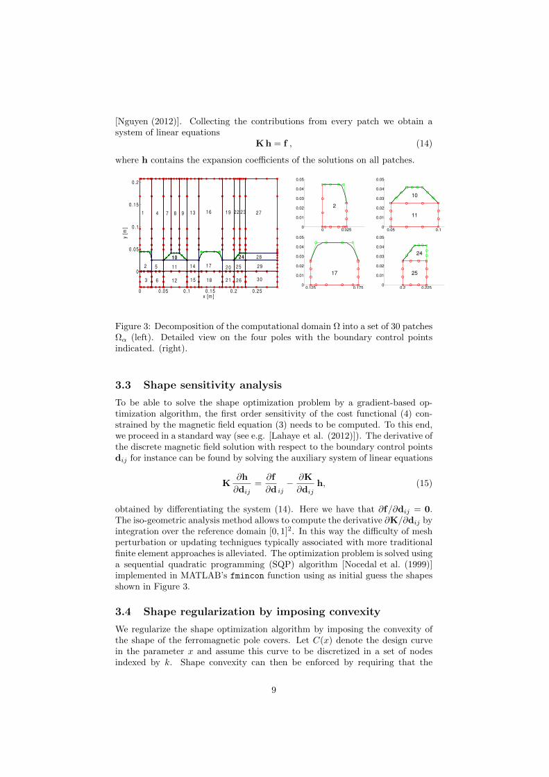
The IGA method employs the same basis functions to represent both the ge-ometry and the discrete solution of the field equation. In this way the methodis similar to the iso-parametric finite element method. The IGA method how-ever uses a more global parametrization of the geometry than classical finiteelement methods by decomposing the computation domain into a set of patchesΩ = ∪αΩα. Such a decomposition for the magnetic density separator shownin Figure 2(a)-(b) into a set of 30 patches is shown in Figure 3. In this fig-ure, the ferromagnetic poles with patch number 2 and 17 are parametrized asa single patch while the magnetic poles with patch number 10, 11, 24 and 25are parametrized using two patches to allow the ferromagnetic caps to cover themagnets. Patches number 3, 6, 12, 15, 18, 21 and 26 and the remaining patchescorrespond to the ferromagnetic back plate and the air region, respectively. Thetop boundary of the ferromagnetic and magnetic poles will be allowed to changeduring the shape optimization process. The global handling of the geometry bypatches will facilitate adopting the discretization to changes in the geometry inthe next section.

Given the well-documented versatility of splines for representing complexshapes, the IGA method uses these functions as basis functions. In this workwe adopt B-splines. Let u and v denotes the coordinates in the parameter space[0, 1]2. Let h denote the mesh width of an equidistant mesh on [0, 1], and leti and j denote the numbering of the basis functions in the x and y direction,respectively. We will parametrize the patch Ωα using B-splines of order p andq with knot vectors Ξαu and Ξαv denoted by Mα,p

i (u) and Nα,qj (v), respectively.

Given the knot vector

Ξαu = 0, . . . , 0︸ ︷︷ ︸p+ 1 times

, h, 2h, . . . , 1− 2h, 1− h, 1, . . . , 1︸ ︷︷ ︸p+ 1 times

, (7)

the set of splines Mα,pi (u) is constructed as a linear combination of products of

lower order splines. A similar argument holds for the construction Nα,qj (v) given

Ξαv . We will expand the discrete solution on a patch using the same B-splines.We will denote the tensor product of splines by Rα,pqij (u, v) = Mα,p

i (u)Nα,qj (v).

Each patch Ωα is parametrized by a linear combination of tensor productsof the geometry splines, i.e., Fα : [0, 1]2 → Ωα where

Fα(u, v) =(xα(u, v), yα(u, v)

)=

m∑i=1

n∑j=1

dij Rα,pqij (u, v) , (8)

where dij are the control points. To highlight the dependence of Fα(u, v) onthe control points, we will use the notation Fα(u, v; d). We use spline degreep = 3 = q on all patches. We will distinguish between patches whose shape isfixed and variable during the design process. On the latter patches, we will treatthe boundary and interior control points separately. To control the shape of theboundary of a design-variable patch, we perform a uniform h → H coarseningof the corresponding knot vector (7) to obtain

Ξαu = 0, . . . , 0︸ ︷︷ ︸p+ 1 times

, H, 2H, . . . , 1− 2H, 1−H, 1, . . . , 1︸ ︷︷ ︸p+ 1 times

, (9)

7

and designate the x and y-coordinates of the corresponding control points asdesign variables. In this construction knot vectors required for the boundaryparametrization of Fα are obtained by inserting points uniformly in the knotvector used to describe shape variations. Consequently, the boundary controlpoints are linear combinations of the design control points. This allows to updateof the parametrization of an entire patch to shape variations of its boundaryand is the distinct feature of the shape optimization using IGA method. Thisprocedure will be outlined in more details in the next section. Figure 3 illustratesthis division in control points for the patches corresponding to the magnet (α =10, 11, 24, 25) and ferromagnetic (α = 2, 17) poles. The y-coordinate of thevariable boundary control points of patch number 2, 7, 10 and 24 add up to atotal of 23 design variables.

3.2 Field Equation Discretization

On each patch the basis functions are defined by composing the inverse of theparametrization Fα (also referred to as the pull-back operator) with the tensorof two analysis splines to obtain Rα,pqij F−1

α (x, y). The discrete approximationu(x, y) to the magnetic vector potential over Ωα can be expanded in this basisas

u(x, y) =

m∑i

n∑j

hαijRα,pqij F−1

α (x, y) . (10)

To determine the expansion coefficients hαij , we proceed as in any classical finiteelement method and cast the magnetic field equation (3) in a Galerkin vari-ational formulation. The resulting integrals over Ωα can be transformed intointegrals over [0, 1]2∫∫

Ωα

f(x, y)dx dy =

∫ 1

0

∫ 1

0

f(xα(u, v), yα(u, v)

)det(Jα) du dv , (11)

where Jα = ∂Fα/∂(u, v) denotes the Jacobian of Fα, and evaluated via Gaus-sian quadrature. The weak form on Ωα then leads to the system of algebraicequations Kα hα = fα, where hα contains the coefficients hαij . The entries ofKα are of the form

Kαk,` =

1

µ

∫ 1

0

∫ 1

0

(∇Rk J−1

α

)T (∇R` J−1α

)det Jα dudv , (12)

where the indices k and ` correspond to a lexicografic ordering of the unknowns.Given that patches number 11 and 25 are formed by vertically magnetized mag-nets of size hm and with magnetization M0, the entries of fα are of the form

fα` =

M0 hm

∫ 1

0(R`(1, v)−R`(0, v)) dv if α = 11 or α = 25 ,

0 otherwise .(13)

Imposing the continuity of both the domain parametrization and the field so-lution along the patch boundaries results in linear dependencies of a num-ber of control points and expansion coefficients corresponding to neighbouringpatches. These can easily be eliminated from the final system as detailed in

8

[Nguyen (2012)]. Collecting the contributions from every patch we obtain asystem of linear equations

K h = f , (14)

where h contains the expansion coefficients of the solutions on all patches.

0 0.05 0.1 0 .15 0.2 0 .25

0

0.05

0.1

0 .15

0.2

x [m ]

y [

m]

1

30

29

28

27

26

25

24

2322

21

20

19

18

17

16

15

14

13

12

11

10

987

6

5

4

2

3

0 0.0250

0.01

0.02

0.03

0.04

0.05

2

0.05 0.10

0.01

0.02

0.03

0.04

0.05

10

11

0.125 0.1750

0.01

0.02

0.03

0.04

0.05

17

0.2 0.2250

0.01

0.02

0.03

0.04

0.05

24

25

Figure 3: Decomposition of the computational domain Ω into a set of 30 patchesΩα (left). Detailed view on the four poles with the boundary control pointsindicated. (right).

3.3 Shape sensitivity analysis

To be able to solve the shape optimization problem by a gradient-based op-timization algorithm, the first order sensitivity of the cost functional (4) con-strained by the magnetic field equation (3) needs to be computed. To this end,we proceed in a standard way (see e.g. [Lahaye et al. (2012)]). The derivative ofthe discrete magnetic field solution with respect to the boundary control pointsdij for instance can be found by solving the auxiliary system of linear equations

K∂h

∂dij=∂f

∂d ij− ∂K

∂dijh, (15)

obtained by differentiating the system (14). Here we have that ∂f/∂dij = 0.The iso-geometric analysis method allows to compute the derivative ∂K/∂dij byintegration over the reference domain [0, 1]2. In this way the difficulty of meshperturbation or updating technigues typically associated with more traditionalfinite element approaches is alleviated. The optimization problem is solved usinga sequential quadratic programming (SQP) algorithm [Nocedal et al. (1999)]implemented in MATLAB’s fmincon function using as initial guess the shapesshown in Figure 3.

3.4 Shape regularization by imposing convexity

We regularize the shape optimization algorithm by imposing the convexity ofthe shape of the ferromagnetic pole covers. Let C(x) denote the design curvein the parameter x and assume this curve to be discretized in a set of nodesindexed by k. Shape convexity can then be enforced by requiring that the

9

second derivative d2C/dx2 remains negative. The second order central finitedifference discretization of this derivative on the set of nodes results in the setof inequalities

Ck+1 − 2Ck + Ck−1 ≤ 0 (16)

that are added to the shape optimization problem. In this way we avoid shapeswith strong oscillations or sharp corners.

4 Domain Parametrization using B-Splines

In this section we discuss the techniques that we employ to construct a parametriza-tion Fα defined in (8) of a patch Ωα that is both invertible and of sufficientlyhigh quality. Given the parametrization of the boundary of Ωα that typicallyresults from a shape updating step in the optimization process, our goal is tocompute the control points d corresponding to the interior control points thatsatisfy both requirements on Fα. The difficulty of this task increases with thegeometrical complexity of Ωα. Given that the procedures to find d have to beapplied within each step of an outer optimization algorithm, it is of paramountimportance to keep their computational complexity limited.

To ensure regularity of Fα(u, v) we require that given some ε > 0, theJacobian Jα(u, v) satisfies det(Jα(u, v)) ≥ ε for all (u, v) ∈ (0, 1)2. We denoteby det[dij ,dk`] the determinant of the 2 × 2 matrix formed by the x and y-coordinates of dij and dk`. Differentiating (8), we obtain

det(Jα(u, v)) =

m∑i,j=1

n∑k,`=1

det[dij ,dk`]dMα,p

i (u)

duNα,qj (v)Mα,p

k (u)dNα,q

` (v)

dv

=

2m−1∑i=1

2n−1∑j=1

cijMα,2p−1i (u)Nα,2q−1

j (v) ,

(17)where Mα,2p−1

i (u) and Nα,2q−1j (v) are B-splines of order 2p− 1 and 2q− 1 over

the patch Ωα, respectively, and where to each of the coefficients cij correspondsa quadratic form determined by the square symmetric matrix Qij such that[Piegl et al. (1997)]

cij = dTQijd . (18)

Given that the B-splines are positive, the regularity of Fα(u, v) can be ensuredby imposing that each of the coefficients cij in (17) is positive.

To ensure that a parametrization Fα is of high quality we require the matrixgα = JTαJα to be well approximated by the identity (see e.g. Corollary 6.4.3 in[Pressley (2010)]). To this end we introduce the Winslow functional W [Fα(d)][Knupp et al. (1993)] defined by

W [Fα(d)] =

∫∫[0,1]2

W[Fα(u, v; d)] du dv , (19)

where for over (u, v) ∈ (0, 1)2 the integrand W[Fα(u, v; d)] is given by

W[Fα(u, v; d)] =trace(gα)√

det(gα)=λ1 + λ2√λ1λ2

=‖∂Fα/∂u‖2 + ‖∂Fα/∂v‖2

det(Jα), (20)

10

and where λ1 and λ2 denote the eigenvalues of gα. A high quality of Fα thencorresponds to as low value of W [Fα(d)] as possible. Minimizing W [Fα(d)]over the feasible set of control points d that yield positive coefficients cij ishowever too computationally demanding to be carried out at every step of theouter optimization algorithm. We therefore resort to a two-stage heuristic thatis described below.

4.1 Constructing and Updating the Parametrization

In the first stage we construct a reference parametrization denoted by d0 byminimizing the Winslow functional (19) over the design space of spline controlpoints d subject to the constraint that the coefficients cij defined by (18) remainpositive. This optimization problem is solved to local optimality using a non-linear optimization method, in fact the same as we use in the outer optimization.

In the second stage we update the parametrization d to the current shape ofthe patch Ωα by minimizing the second order Taylor polynomial of the Winslowfunctional (19) around the point d0. This polynomial can be written as

W [Fα(d)] ≈W [Fα(d0)] +G(d0)(d0 − d) + 1/2(d0 − d)TH(d0)(d0 − d) , (21)

where G(d0) and H(d0) denote the gradient and Hessian of W [Fα] with respectto the control points d evaluated in the point d0, respectively. Minimizing thispolynomial is then equivalent to solving the linear system of equations

H(d0)(d0 − d) = −G(d0) , (22)

resulting in an inexpensive updating formula. At the same time the positivityof coefficients cij is added as constraints in the outer optimization thus ensuringa valid parametrization throughout the outer optimization. At the end of theparametrization we check if the constraint on any of the coefficients cij is active.If one of them is, then the reference parametrization d0 is update in a processsimilar to remeshing in standard finite element methods and we restart the outerparametrization.

5 Numerical experiments

This section consists of two subsections. In Subsection 5.1 we validate our iso-geometric shape optimization algorithm on a synthetic problem for which ananalytical expression for the optimal shape is known. In Subsection 5.2 wesolve the design problem of the magnet array shown in Figure 2 (a)-(b).

5.1 Synthetic Problem with Analytical Expression for theOptimal Shape

In this subsection we show that in the absence of end effects the analyticalexpression for the optimal shape of the pole cover given in [Lahaye et al. (2011)]can be derived. We first give a concise derivation of the optimal shape thatthis reference lacks. We subsequently employ this shape to investigate at whatrate the difference between the numerically and analytically determined shapesconverges to zero as the meshwidth is decreased. We do so for various polynomialorders of the spline approximation.

11

To derive the analytical expression for the optimal shape, we consider firstthe magnetic field generated above an idealized Hallbach magnet array of heighthm that extends to infinity in lateral directions. We assume the magnet tobe mounted on a ferro-magnetic plate reducing the problem to computing themagnetic field caused by the magnet strip (x, y, z) | − ∞ ≤ x ≤ ∞,−hm ≤y ≤ 0,−∞ ≤ z ≤ ∞ in the overlying half-space (x, y, z) | − ∞ ≤ x ≤∞, 0 ≤ y,−∞ ≤ z ≤ ∞. We assumed the magnet to be magnetized inthe y-direction in such a way that, given some amplitude M0 and given somewavelength λ, the magnet’s pre-magnetization vector M can be written asM = (0,M0 cos(πx/λ), 0). The problem is thus reduced to the coordinatesx and y. Let µr denote the magnet’s permeability. To solve the magnetic fieldproblem in the magnet and air region, we solve the Laplace equation for scalarmagnetic potential φ(x, y) supplied with appropriate boundary and interfaceconditions. The latter are applied on the line y = 0. We proceed in a similarway to what for example [Cho et al. (2001)] refers to as Type (a) magnet arraysand find that in magnet region the scalar potential varies linearly with y. Inthe air region holds that

φ(x, y) = C1 cos(π x/λ) exp(−π y/λ) , (23)

where C1 is an integration constant equal to

C1 =M0 hm

µr + πhm/λexp(

πhmλ

) . (24)

The magnetic field strength in the region above the magnet is therefore givenby

‖B‖ = µ0

√(∂φ/∂x)2 + (∂φ/∂y)2 = µ0C1π/λ exp(−π y/λ) , (25)

and trivially satisfies Condition (2). In the derivation above, end-effect wereneglected.

Hallbach arrays for magnetic density separation have been proposed in lit-erature [Svoboda (2004)]. To reduce the amount of magnetic material usedhowever, a new design in which magnets magnetized in only upward directionand in which the magnet poles are interleaved with iron poles has been pro-posed in [Lahaye et al. (2011)]. In this design the magnetic field distributionabove the poles is brought into the desired shape by covering both the iron andmagnetic poles with iron parts as shown in Figure 1. On the air boundary ofthese ferromagnetic coverings the magnetic flux only has a normal component.The tangential component and therefore the tangential derivative of the scalarmagnetic potential is zero on this boundary. This implies that on this boundarythe magnetic scalar potential is constant. The optimal shape for this coveringis thus known as soon as a scalar potential for the optimal field is known. Thisoptimal scalar potential is given by (23) assuming no end-effects are present.The optimal shape is thus found by setting φ(x, y) equal to a constant φ0 andmaking the relationship between x and y explicit to obtain

Canal(x) =λ

πlog[cos(

π x

λ)] + C2 , (26)

where C2 = λ/π(logC1 − log φ0). This curve was used to shape the pole coversin Figure 1. In [Lahaye et al. (2011)] is was verified numerically that a peri-odic continuation of the configuration shown in Figure 1 does give the a fielddistribution satisfying Condition (2).

12

In the remainder of this subsection we consider a synthetic shape optimiza-tion algorithm that has the curve (26) as optimal solution. Our aim is toinvestigate the rate of convergence of the numerically computed solution to theexact one as function of meshwidth H used to discretize the design curve andof the polynomial degree p of the spline approximation To this end we define,given y(x) a smooth function in x and y = 0.2077 m, the computational domainΩp = (x, y) | − λ/3 ≤ x ≤ λ/3, y(x) ≤ y ≤ y representing the air domainabove a single magnetic pole. On this domain we consider solving the Laplaceequation for the scalar potential φ subject to the exact solution (23) given onthe boundary. The goal of the synthetic shape optimization algorithm is tominimize the functional

J0[φ;D] =

∫D

(∂‖B‖∂x

)2

dx dy (27)

(measured in T 2) where D = [−0.02, 0.02]× [0.06, 0.12] [m×m] by varying theshape of y(x). Motivating this choice for J0[φ;D] is that if ∂x‖B‖ = 0 thenautomatically ∂x(∂y‖B‖) = ∂y(∂x‖B‖) = 0 and Condition (2) is satisfied. Theevaluation of this cost functional requires second order derivatives of the scalarpotential φ. The curve Canal(x) is given by (26) is the analytical solution to thisdesign problem. Let Copt(x) denote its approximation computed numericallyby the IGA shape optimization algorithm on the discretization defined by thefollowing geometry knot vectors

Ξu = 0, . . . , 0︸ ︷︷ ︸p+ 1 times

, 132 , . . . ,

3132 , 1, . . . , 1︸ ︷︷ ︸

p+ 1 times

Ξv = 0, . . . , 0︸ ︷︷ ︸q + 1 times

, 15 , . . . ,

45 , 1, . . . , 1︸ ︷︷ ︸q + 1 times

.

(28)We compute the scaled L2-norm of the difference between Copt(x) and Canal(x)for H ∈ 1

2 ,14 ,

18 ,

116 ,

124, p ∈ 2, 3, 4 and q = p. For p = 3, the afore mentioned

choices of H leads to a problem with the number of design variables Ndv equalto Ndv ∈ 3, 5, 7, 9, 17, 25. Results are given in Figure 4.

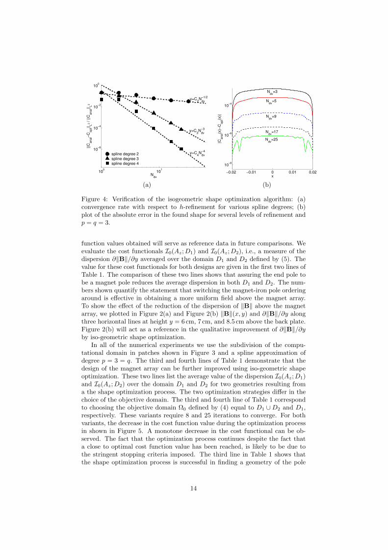
Figure 4 (a) shows how the scaled L2-norm of error in the computed designcurve ‖Canal(x) − Copt(x)‖2/‖Canal(x)‖2 decreases with the number of designvariables Ndv for the three polynomial degrees. This figure shows that for p = 2the error scales as O(H1/2) and that for p = 3 and p = 4 the error scales asO(Hp). The latter rate is not to be confused with the classical estimate ofO(Hp+1) that holds for errors computed over the entire computational domainthat remains fixed during the convergence study. A theoretical framework ex-plaining the observed rate of convergence is in fact not known to the authors.The extension of this synthetic problem in which the cost functional (27) is re-placed by (4) as well as the development of the required framework that explainsthe observed rates is left for further work.

5.2 Shape Optimization of Pole Covers of Magnetic Den-sity Separators

Before describing the application of the iso-geometric shape optimization algo-rithm to the density separator, we evaluate the cost functional (4) on the designproposed in [Lahaye et al. (2011)] with the original and reversed pole order-ing. These designs are shown in Figure 1 and Figure 2, respectively. The cost

13

100

101

10−6

10−4

10−2

100

Ndv

||C

anal−

Copt||

L2 /

||C

anal||

L2

spline degree 2spline degree 3spline degree 4

y=C3N

dv

−3

y=C4N

dv

−4

y=C2N

dv

−1/2

−0.02 −0.01 0 0.01 0.02

10−8

10−6

10−4

x

|Ca

na

l(x)−

Co

pt(x

)|

Ndv

=25

Ndv

=17

Ndv

=9

Ndv

=5

Ndv

=3

(a) (b)

Figure 4: Verification of the isogeometric shape optimization algorithm: (a)convergence rate with respect to h-refinement for various spline degrees; (b)plot of the absolute error in the found shape for several levels of refinement andp = q = 3.

function values obtained will serve as reference data in future comparisons. Weevaluate the cost functionals I0(Az;D1) and I0(Az;D2), i.e., a measure of thedispersion ∂‖B‖/∂y averaged over the domain D1 and D2 defined by (5). Thevalue for these cost functionals for both designs are given in the first two lines ofTable 1. The comparison of these two lines shows that assuring the end pole tobe a magnet pole reduces the average dispersion in both D1 and D2. The num-bers shown quantify the statement that switching the magnet-iron pole orderingaround is effective in obtaining a more uniform field above the magnet array.To show the effect of the reduction of the dispersion of ‖B‖ above the magnetarray, we plotted in Figure 2(a) and Figure 2(b) ‖B‖(x, y) and ∂‖B‖/∂y alongthree horizontal lines at height y = 6 cm, 7 cm, and 8.5 cm above the back plate.Figure 2(b) will act as a reference in the qualitative improvement of ∂‖B‖/∂yby iso-geometric shape optimization.

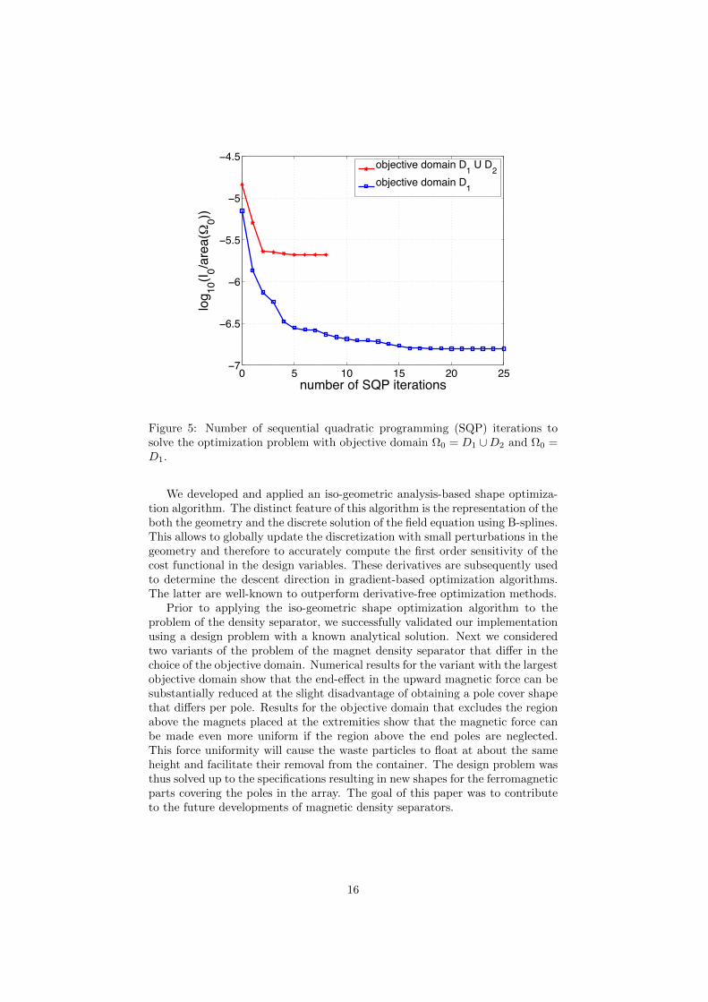
In all of the numerical experiments we use the subdivision of the compu-tational domain in patches shown in Figure 3 and a spline approximation ofdegree p = 3 = q. The third and fourth lines of Table 1 demonstrate that thedesign of the magnet array can be further improved using iso-geometric shapeoptimization. These two lines list the average value of the dispersion I0(Az;D1)and I0(Az;D2) over the domain D1 and D2 for two geometries resulting froma the shape optimization process. The two optimization strategies differ in thechoice of the objective domain. The third and fourth line of Table 1 correspondto choosing the objective domain Ω0 defined by (4) equal to D1 ∪D2 and D1,respectively. These variants require 8 and 25 iterations to converge. For bothvariants, the decrease in the cost function value during the optimization processin shown in Figure 5. A monotone decrease in the cost functional can be ob-served. The fact that the optimization process continues despite the fact thata close to optimal cost function value has been reached, is likely to be due tothe stringent stopping criteria imposed. The third line in Table 1 shows thatthe shape optimization process is successful in finding a geometry of the pole

14

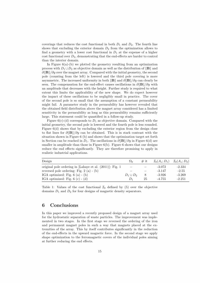
coverings that reduces the cost functional in both D1 and D2. The fourth lineshows that excluding the exterior domain D2 from the optimization allows tofind a geometry with a lower cost functional in D1 at the expense of a highercost functional over D2, demonstrating that the end-effects are harder to controlthan the interior domain.

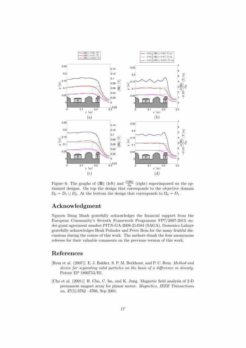
In Figure 6(a)-(b) we plotted the geometry resulting from an optimizationprocess with D1∪D2 as objective domain as well as the distribution of ‖B‖ and∂‖B‖/∂y over the magnet array. Compared with the initial geometry, the secondpole (counting from the left) is lowered and the third pole covering is moreasymmetric. The increased uniformity in both ‖B‖ and ∂‖B‖/∂y can clearly beseen. The compensation for the end-effect causes oscillations in ∂‖B‖/∂y withan amplitude that decreases with the height. Further study is required to whatextent this limits the applicability of the new shape. We do expect howeverthe impact of these oscillations to be negligibly small in practice. The coverof the second pole is so small that the assumption of a constant permeabilitymight fail. A parameter study in the permeability has however revealed thatthe obtained field distribution above the magnet array considered has a limitedsensitivity in the permeability as long as this permeability remains sufficientlylarge. This statement could be quantified in a follow-up study.

Figure 6(c)-(d) corresponds to D1 as objective domain. Compared with theinitial geometry, the second pole is lowered and the fourth pole is less rounded.Figure 6(d) shows that by excluding the exterior region from the design closeto flat lines for ∂‖B‖/∂y can be obtained. This is in stark contrast with thesituation shown in Figure 6 (b) and shows that the optimization target set forthin Section can be reached in D1. The oscillations in ∂‖B‖/∂y in Figure 6(d) aresmaller in amplitude than those in Figure 6(b). Figure 6 shows that our designsreduce the end effects significantly. They are therefore promising to apply inrealistic industrial applications.

Design Ω0 # it I0(Az;D1) I0(Az;D2)

original pole ordering in [Lahaye et al. (2011)]: Fig. 1 − − -3.072 -2.334reversed pole ordering: Fig. 2 (a) - (b) − − -3.147 -2.55IGA optimized: Fig. 6 (a) - (b) D1 ∪D2 8 -3.926 -3.269IGA optimized: Fig. 6 (c) - (d) D1 25 -4.755 -2.251

Table 1: Values of the cost functional I0 defined by (5) over the objectivedomains D1 and D2 for four designs of magnetic density separators.

6 Conclusions

In this paper we improved a recently proposed design of a magnet array usedfor the hydrostatic separation of waste particles. The improvement was imple-mented in two stages. In the first stage we reversed the ordering of the ironand permanent magnet poles in such a way that magnets placed at the ex-tremities of the array. This by itself contributes significantly in the reductionof the end-effects in the upward magnetic force. In the second stage we applyshape optimization to the ferromagnetic covers of the individual poles aimingat further reducing the end effects.

15

0 5 10 15 20 25−7

−6.5

−6

−5.5

−5

−4.5

number of SQP iterations

log 10

(I0/a

rea(Ω

0))

objective domain D1 U D

2

objective domain D1

Figure 5: Number of sequential quadratic programming (SQP) iterations tosolve the optimization problem with objective domain Ω0 = D1 ∪D2 and Ω0 =D1.

We developed and applied an iso-geometric analysis-based shape optimiza-tion algorithm. The distinct feature of this algorithm is the representation of theboth the geometry and the discrete solution of the field equation using B-splines.This allows to globally update the discretization with small perturbations in thegeometry and therefore to accurately compute the first order sensitivity of thecost functional in the design variables. These derivatives are subsequently usedto determine the descent direction in gradient-based optimization algorithms.The latter are well-known to outperform derivative-free optimization methods.

Prior to applying the iso-geometric shape optimization algorithm to theproblem of the density separator, we successfully validated our implementationusing a design problem with a known analytical solution. Next we consideredtwo variants of the problem of the magnet density separator that differ in thechoice of the objective domain. Numerical results for the variant with the largestobjective domain show that the end-effect in the upward magnetic force can besubstantially reduced at the slight disadvantage of obtaining a pole cover shapethat differs per pole. Results for the objective domain that excludes the regionabove the magnets placed at the extremities show that the magnetic force canbe made even more uniform if the region above the end poles are neglected.This force uniformity will cause the waste particles to float at about the sameheight and facilitate their removal from the container. The design problem wasthus solved up to the specifications resulting in new shapes for the ferromagneticparts covering the poles in the array. The goal of this paper was to contributeto the future developments of magnetic density separators.

16

0 0.2 0.4 0.6 0.8 10

0.2

0.4

0.6

0.8

1

‖B‖(x, 0.06) [T]‖B‖(x, 0.07) [T]‖B‖(x, 0.085) [T]

0 0.2 0.4 0.6 0.8 10

0.2

0.4

0.6

0.8

1

−0.05 ∂∂y‖B‖(x, 0.06) [T/m]

−0.05 ∂∂y‖B‖(x, 0.07) [T/m]

−0.05 ∂∂y‖B‖(x, 0.085) [T/m]

0 0.1 0.2 0.3

0

0.05

0.1

0.15

0.2

0.25

x [m]

y[m

]

−0.02

0

0.02

0.04

0.06

0.08

0.1

0.12

0.14

‖B‖[T

]

0 0.1 0.2 0.3

0

0.05

0.1

0.15

0.2

0.25

x [m]

y[m

]

0

1

2

3

4

5

6

7

−0.05∂‖B‖

∂y

[T/m]

(a) (b)

0 0.1 0.2 0.3

0

0.05

0.1

0.15

0.2

0.25

x [m]

y[m

]

−0.02

0

0.02

0.04

0.06

0.08

0.1

0.12

0.14

‖B‖[T

]

0 0.1 0.2 0.3

0

0.05

0.1

0.15

0.2

0.25

x [m]

y[m

]

0

1

2

3

4

5

6

7

−0.05∂‖B‖

∂y

[T/m]

(c) (d)

Figure 6: The graphs of ‖B‖ (left) and ∂‖B‖∂y (right) superimposed on the op-

timized designs. On top the design that corresponds to the objective domainΩ0 = D1 ∪D2. At the bottom the design that corresponds to Ω0 = D1.

Acknowledgment

Nguyen Dang Manh gratefully acknowledges the financial support from theEuropean Community’s Seventh Framework Programme FP7/2007-2013 un-der grant agreement number PITN-GA-2008-214584 (SAGA). Domenico Lahayegratefully acknowledges Henk Polinder and Peter Rem for the many fruitful dis-cussions during the course of this work. The authors thank the four anonymousreferees for their valuable comments on the previous version of this work.

References

[Rem et al. (2007)] E. J. Bakker, S. P. M. Berkhout, and P. C. Rem. Method anddevice for separating solid particles on the basis of a difference in density.Patent EP 1800753/B1.

[Cho et al. (2001)] H. Cho, C. Im, and K. Jung. Magnetic field analysis of 2-Dpermanent magnet array for planar motor. Magnetics, IEEE Transactionson, 37(5):3762 –3766, Sep 2001.

17

[Cho et al. (2009)] S. Cho and S. Ha. Isogeometric shape design optimiza-tion: exact geometry and enhanced sensitivity. Struct. Multidiscip. Optim.,38(1):53–70, 2009.

[Cottrel et al. (2009)] J. A. Cottrell, T. J. R. Hughes, and Y. Bazilevs. Isoge-ometric Analysis: Toward Integration of CAD and FEA. J. Wiley., WestSussex, 2009.

[Di Barba et al. (2009)] P. Di Barba and M.E. Mognaschi. Industrial designwith multiple criteria: Shape optimization of a permanent-magnet genera-tor. Magnetics, IEEE Transactions on, 45(3):1482 –1485, Mar 2009.

[Hollig (2003)] K. Hollig. Finite Element Methods with B-Splines. Number 26in Frontiers in Applied Mathematics. SIAM, 2003.

[Hughes et al. (2005)] T.J.R. Hughes, J.A. Cottrell, and Y. Bazilevs. Isogeo-metric analysis: CAD, finite elements, NURBS, exact geometry and meshrefinement. Comput. Methods Appl. Mech. Engrg., 194(39-41):4135–4195,2005.

[Kim et al. (2002)] D. Kim, S. Lee, I. Park, and J. Lee. Derivation of a generalsensitivity formula for shape optimization of 2-D magnetostatic systems bycontinuum approach. Magnetics, IEEE Transactions on, 38(2):1125 –1128,Mar 2002.

[Kim et al. (2002)] D.H. Kim, J.K. Sykulski, and D.A. Lowther. The implica-tions of the use of composite materials in electromagnetic device topologyand shape optimization. Magnetics, IEEE Transactions on, 45(3):1154 –1157, Mar 2009.

[Knupp et al. (1993)] P. Knupp and S. Steinberg. Fundamentals of Grid Gen-eration. CRC Press, Boca Ranton, 1993.

[Lahaye et al. (2011)] D. Lahaye, H. Polinder, and P. Rem. Magnet designsfor magnetic density separation of polymers. The Journal of Solid WasteTechnology and Management, 26:977–983, 2011.

[Lahaye et al. (2012)] D. Lahaye and W. Mulckhuyse, (2012) Adjoint sensitiv-ity in PDE constrained least squares problems as a multiphysics problem.COMPEL, 31(3):895–903, 2012.

[Muchova et al. (2009)] Muchova L., E. J. Bakker, and P. Rem. Precious Met-als in Municipal Solid Waste Incineration Bottom Ash. Water Air SoilPollution, 9(1-2):107–116, 2009.

[Nguyen (2012)] D. Manh Nguyen. Isogemetric Analysis and Shape Optimiza-tion in Electromagnetics. PhD thesis, Technical University of Denmark,2012.

[Nguyen et al. (2012)] D.M. Nguyen, A. Evgrafov, and J. Gravesen. Isogeomet-ric shape optimization for electromagnetic scattering problems. Progressin Electromagnetics Research B, 46:117–146, 2012.

[Nocedal et al. (1999)] J. Nocedal and S. J. Wright. Numerical Optimization.Springer Series in Operations Research. Springer, 1999.

18

[Piegl et al. (1997)] L. Piegl and W. Tiller. The NURBS book. Springer-Verlag,New York, NY, USA, second edition, 1997.

[Pressley (2010)] A. N. Pressley. Elementary Differential Geometry. Springer,second edition, 2010.

[Rosensweig (1987)] R. E. Rosensweig. Magnetic fluids. Ann. Rev., 19:437–463,1987.

[Saludjian et al. (1998)] L. Saludjian, J.L. Coulomb, and A. Izabelle. Geneticalgorithm and Taylor development of the finite element solution for shapeoptimization of electromagnetic devices. Magnetics, IEEE Transactionson, 34(5):2841 –2844, Sep 1998.

[Svoboda (2004)] J. Svoboda. Magnetic Techniques for the Treatment of Mate-rials. Kluwer, Dordrecht, The Netherlands, 2004.

[Sylvester et al. (1996)] P. P. Sylvester and R. L. Ferrari. Finite Elements forElectrical Engineers. Cambridge University Press, New York, third edition,1996.

[Tadic et al. (2011)] T. Tadic and B.G. Fallone. Three-dimensional nonaxisym-metric pole piece shape optimization for biplanar permanent-magnet MRIsystems. Magnetics, IEEE Transactions on, 47(1):231 –238, Jan. 2011.

19