Preliminary and Incomplete

Please do not cite

Is Residual Income Really Uninformative About Stock Returns?

by

Sudhakar V. Balachandran*

and

Partha Mohanram*

October 25, 2006

Abstract:

Prior research found that Residual Income (RI) is, at best, minimally informative about stock returns relative to Earnings, despite strong support for RI in theory and among practitioners. We examine three possible explanations for this puzzle. First, the empirical literature ignores some salient feature of practice or theory. Second, the market does not fully impound all of the information from residual income into current returns. Third, the theory abstracts away some real world feature captured in prior empirical results. We find that while the incremental contribution of RI to earnings is modest in explaining current returns, conditioning on whether or not RI increased or decreased affects the relationship between earnings and returns. Further, the market only partially impounds the information in residual income into current returns. A strategy of going long on firms with the greatest increase in RI and short on firms with the greatest decrease in RI generates significant positive excess returns that persist after controlling for risk factors. Our results are consistent with the first two explanations above. Specifically, benchmarking earnings versus the cost of capital is an important feature of how accountants interpret residual income; incorporating this feature of residual income increases the information content of earnings. Furthermore, our results on future returns indicate that tests of the association of changes in RI with current returns present only a partial picture of the usefulness of RI.

We would like to thank Tim Baldenius for his comments. We appreciate research assistance from Columbia Business School. All errors are our own. Please contact Sudhakar Balachandran at svb34@columbia.edu or Partha Mohanram at pm2128@columbia.edu with questions and comments.

1

1. Introduction

This paper re-examines the association between residual income and stock

returns. Ittner and Larcker (2001) discuss this research as part of their review of the

literature on “Shareholder Value Management.” Central to this literature is debate over

which measures of performance organizations should use to incentivize managers to

strive to generate economic value for shareholders. Papers by Biddle, Bowen and

Wallace (1997), and Chen & Dodd (1997) find that residual income has only a minimally

incremental association with stock returns, relative to earnings. Garvey and Milbourn

(2000) develop a principal agent model where the association between a given

performance measure and stock returns is shown to be a proxy for the signal to noise

ratio, which in turn determines the weight of a given measure in a compensation contract

(Banker & Datar 1989). Correspondingly, the lack of association with stock returns

brings the usefulness of residual income as a measure to align the interests of the

principal and the agent (i.e. shareholders and management) into question.

The lack of association between residual income and returns in prior research is

puzzling. First, there is extensive theoretical work (Anctil 1996, Baldenius 2002, Dutta

& Reichelstein 2002, Reichelstein 1997, Rogerson 1997) demonstrating that residual

income is useful in managing decentralized investment decisions within organizations by

ensuring the effectiveness of capital investment. Theory has also discussed the

usefulness of cost of capital as a hurdle rate, a management practice commonly observed

in publicly companies (Simons 2001). Second, prior empirical research (Wallace 1997,

Balachandran 2006) shows that residual income based compensation is associated with

changes in investment behavior. Finally, residual income has been discussed in

2

accounting classes from as early as the 1960’s. Textbooks over the years have discussed

residual income as earnings in excess of the cost of capital employed to generate those

earnings (Solomons 1965, Morse & Zimmerman 1997, Horngren, Datar & Foster 2006).

Given the history of residual income in accounting, we posit three possible

explanations for the puzzling lack of association between residual income and returns.

First, the empirical literature may have ignored some salient feature of practice or theory.

Second, the market may not have fully impounded all of the information from residual

income into current returns. Third, the theory may have abstracted away some real world

feature captured in the empirical results. In our research design, we conduct tests

motivated by the first two explanations. We will interpret the failure to find supporting

evidence for either of the first two explanations as indirect support for the third

explanation. Our research design is built around insights about residual income found in

accounting text books and prior theory.

Textbooks note that earnings can increase simply because the returns from

incremental investments exceed the cost of debt added to the firm. In contrast, since

residual income requires a charge that accounts for the cost of all capital employed,

residual income may not increase even if earnings increase. Hence changes in residual

income combined with increases in earnings may be informative about the nature of the

earnings increases, and correspondingly, the actions taken by management. Accordingly,

in this paper we examine changes in earnings and changes in residual income in

examining current stock returns, measures of investment and future returns.

In our research design, we measure earnings as net income before extraordinary

items. We measure residual income as operating earnings (NOPAT) less a charge for the

3

cost of capital employed, where NOPAT is defined as net income plus the after tax cost

of debt. These definitions are consistent with Biddle, Bowen and Wallace (1996).

Further, our approach considers cost of capital as a hurdle rate. Firms commonly use

hurdle rates as part of their capital budgeting process, so a specification which

incorporates this institutional detail may out perform specification which ignore it. We

examine contemporaneous levels stock returns in excess of market, changes in invested

capital and associations between earnings and returns. Specifically we examine the

association between changes in earnings and returns conditioned on changes in residual

income. Because accounting information may not be fully impounded in current stock

prices, we also conduct tests of future returns in excess of market.

Overall we find that depending on whether residual income increased or

decreased, firms with increasing earnings exhibit systematic differences in invested

capital, contemporary returns, future returns, and the association between returns and

earnings. We interpret these results as consistent with residual income and earnings

being jointly informative of shareholder returns. In particular, changes in residual

income facilitate identifying the likelihood that earnings increases are the result of

increasing investment which does not cover the cost of capital employed. Our results

suggest that such investments dampen current returns and the contemporaneous

association between earnings and returns.

Further our results suggest that contemporaneous returns do not fully impound the

implications of earnings which do not exceed the cost of capital, as changes in current

residual income and invested capital predict future returns. We find that firms with the

highest changes in residual income have the greatest 1-year-ahead market-adjusted

4

returns. A strategy of going long in firms with the greatest increases in RI and going

short in firms with the greatest decline in RI earn positive and significant excess returns

that persist after controlling for risk.

Summarizing our results, we conclude that the weak results of prior research can

be attributed to the first two of our three potential explanations. Prior research viewed

earnings and residual income as competing measures, while in practice, residual income

essentially applies a threshold that earnings have to meet given the amount of capital

invested. Further, prior research only tested the association of earnings and residual

income with contemporaneous returns. Our results indicate that the market only partially

impounds the information in changes in residual income in current returns, something

which is corrected in future return realizations. This makes it less likely that the

theoretical research has abstracted away from some critical feature of practice that makes

is un-descriptive of the empirical realities of residual income use.

The remainder of this paper is structured as follows. Section 2 presents our

research question and hypotheses. Section 3 outlines our research design. Section 4

describes our sample selection and provides descriptive statistics. Section 5 presents our

test results. Section 6 concludes.

2. Research Question and Hypotheses

Historically, accountants have raised concerns that earnings from the income

statement should be interpreted with caution, as the income statement does not include a

charge for the cost of capital contributed by equity holders. As a result, income could be

both positive and increasing, but still not provide shareholders with an adequate return.

5

“The cost of debt financing is charged against earnings in the form of interest

expense on existing debt, however there is no corresponding charge against earnings

for equity financing. Any project that is expected to earn greater than the embedded

cost of debt increases the absolute level of earnings but reduces shareholder wealth

unless it also earns greater than the firm’s opportunity cost of all (debt and equity)

capital.” (Wallace 1997)

Further concerns have been raised that managers with compensation targets based

on earnings might invest in projects that cover incremental interest expenses (the cost of

debt), but not their total incremental cost of capital.

“It (earnings based compensation), fails to reflect additional investments; thus profits

and consequently bonuses can increase simply due to new investments, even though

the performance of executives may be static or deteriorating” (Dearden 1972)

Using a principle agent model, Garvey and Milbourn (2000) demonstrate that the

extent to which a given performance measure co-varies with stock returns determines the

optimal weight placed on that measure in incentive contracts. In their model, a risk

neutral principal is interested in maximizing the returns on her stock; hence using the

stock price to provide incentives is desirable. In their model, stock prices are increasing

in the level of action taken by the agent, with noise. Correspondingly, basing the agent’s

incentives purely on stock price imposes risk on a risk-averse agent, which in a first best

world is inefficient. If, however, there are other performance measures (for example,

earnings or residual income) that are also increasing in action with noise, then the extent

of co-variation between the noise terms in stock price and the respective performance

measures determines the weights on these measures in compensation contracts. The co-

variation of noise terms can be viewed as the association between a given performance

6

measure and stock returns; hence the model provides a contracting based motivation to

examine the association between alternate performance measures and returns.

To date, papers that examine the association between residual income, earnings

and stock returns (Biddle, Bowen and Wallace 1997, Chen & Dodd 2000) have found

very little association, which following the Garvey and Milbourn model suggests that

these measures have little use in providing incentives. This lack of association is

puzzling given the history of these measures in practice in accounting, the large body of

theoretical literature on managing investment decisions, and empirical studies

documenting the association between residual income and changes investment (Wallace

1997, Balachandran 2006).

We consider three possible explanations for the lack of association documented in

prior research. First, the extant empirical literature ignores some salient feature of

practice or theory. Second, the market does not fully impound all information in residual

income into current returns. Third, the theory abstracts away some real world feature

captured in the empirical results. We test the first two explanations directly in this paper.

Past empirical research focused on the co-variation between returns and earnings

or residual income in aggregate and the incremental contribution of each. These tests

essentially viewed earnings and residual income as competing measures and ran horse-

race tests pitting these measures against each other. We consider an alternative approach

motivated by historical accounting arguments and past theoretical research. Our

approach focuses on the cost of capital as a hurdle rate, and the salient fact that residual

income increases when the incremental returns from a firm’s operations exceed the

incremental cost of capital employed. Our approach is consistent with the historical

7

arguments that increasing earnings could be misleading, as well as theoretical research

which focuses on using hurdle rates as mechanisms to manage investment decisions in

decentralized settings (Anctil 1996, Baldenius 2002, Dutta & Reichelstein 2002,

Reichelstein 1997, Rogerson 1997).

In summary, theory and textbook arguments suggest that increasing earnings can

have very different implications for shareholders depending on whether those earnings

come with concurrent increases in residual income or not. We use these arguments to

hypothesize consistent with our first possible explanation that:

(H1) Changes in earnings will have a different contemporaneous association with

stock returns depending on concurrent changes in residual income.

Further to the extent that the stock market does not fully and quickly impound the

implications of differences in changes in earnings vs. residual income, we hypothesize

that:

(H2) Changes in residual income can be used to predict future market returns.

3. Research Design

The aim of this paper is to examine the associations between earnings, residual

income and returns. In this section, we outline our research design. We first discuss the

differences between the research design in this paper and prior research. We then

describe the measures used in the paper and discuss the tests using both contemporaneous

as well as future returns.

8

3.1. Our research design vs. prior research

Our research design views informativeness differently than prior literature.

Essentially prior research viewed these measures as competing in a race to explain

returns. We do not necessarily see these measures as competitors, but rather that one

builds off the other, and hence may be informative in specific contexts and scenarios.

Historically accounting texts have viewed the charge for capital as the central

difference between earnings and residual income (RI). This charge is designed to

indicate situations in which returns form the firms’ investment decisions exceed the cost

of debt, but not the total cost of capital.

The theory on using residual income to manage investment decisions often views

the capital charge as a hurdle rate based approach to manage investments. Under

different conditions the theory predicts that firms will use hurdle rates to manage

decentralized investment decisions. It also predicts that the optimal hurdle rate may be

different form the cost of capital, either higher or lower, under different conditions. Our

tests seek to specifically examine the role of the cost of capital measure and use cost of

capital as a hurdle rate in structuring our tests.

Positive RI reflects profits in excess of the required rate of return for total

invested capital, which creates wealth for the shareholders. Negative RI dissipates

shareholder wealth. A firm with exactly zero RI just breaks even with respect to

generating wealth for its shareholders. In our analyses, our emphasis is on the change in

residual income. Assuming that the rate of return from existing projects remains constant,

a firm will generate an increase in residual income if and only if the returns from

9

additional investments also exceed the cost of capital. Changes in residual income reflect

the efficiency of additional investment made in a given year.

3.2. Performance measures

Central to our analysis is the measurement of residual income. Prior research

used data on residual income and EVATM purchased from Stern Stewart, a consulting

firm. In this paper we measure residual income from publicly available information

using an approach based both in the theory of residual income and consistent with the

approach used by consulting firms.1

Consistent with BBW, we start with Net Income before extra-ordinary items (NI).

Next, we define net operating profits after tax (NOPAT) as NI plus the after-tax cost of

interest expense.

NOPAT = NI (#18) + (1-tax rate)* Interest Expense (#15)

We use the prevailing statutory tax rate for each year as our measure of the tax

rate. Consistent with BBW, we set the tax rate to zero if a firm has net operating loss

carry-forwards (NOLs). Our variable of interest is residual income, which focuses on

operating performance net of a charge for capital employed.

RI = NOPAT – k*Capital

where

k = our estimate of the firm’s weighted average cost of capital (wacc). We

calculate wacc by i) estimating a CAPM cost of equity using 60 past months of

returns, ii) inferring after-tax cost of debt from interest expense, total interest

1 Our discussions with consulting firms indicate that our approach is consistent with the approach they use in measurement at firms and with the data they typically sell.

10

bearing debt and the tax rate, and iii) estimating proportions of debt and equity

using market value of equity and book value of total debt.2

Capital = Total Invested Capital (#37)

The main advantage of our approach is that it allows us to examine a longer

period of time and a larger sample of firms than prior research. In our analysis, we focus

on a thirty year period from 1975 to 2004 using information on all December fiscal year-

end firms on Compustat. BBW, on the other hand, focus on a subset of 773 firms from

the 1000 largest firms as measured by market capitalization, and only on the period from

1983 to 1994, using private information supplied by Stern Stewart. Our tests are likely to

have greater power, be more generalizable and importantly, more easily replicable.

Contemporaneous annual returns for a given firm are calculated by compounding

CRSP monthly returns, beginning four months after the beginning of the fiscal year and

ending 12 months thereafter. We do this to allow enough time for firms to close their

annual books and announce earnings. Similarly, one-year-ahead returns are calculated by

starting the compounding period four months after the end of the fiscal year.3 We adjust

the returns by subtracting the return on the value weighted index over the same period.

Note that the market adjustment plays no role in our hedge return results, as all portfolios

are formed at the same period of time, as we focus only on December fiscal year firms.

3.3. Contemporaneous tests

We examine the levels of contemporaneous returns and associations among

returns, earnings and residual income. We examine specifications that are analogous to

2 We estimate betas using at least 24 months of lagged returns. 3 We also examine our main test results using returns measured from fiscal year beginning to end and found consistent results.

11

those of prior research, and introduce new specifications that provide an alternate

interpretation of residual income. Specifically, we first examine regressions similar to

those used in prior research:

Rett = α + β∆Earnt + ε (1)

Rett = α + β∆RIt + ε (2)

Rett = α + β1∆NIt +β2∆RIt + ε (3)

Rett = α + β1∆Earnt + β2∆Intt +β3∆Capchgt + ε (4)

All variables on the right hand side are scaled by lagged assets. We also run the

tests using lagged market value as our scaling variable. Note that the first regression is a

standard earnings response coefficient (ERC) regression. The second regression is an

analog of the ERC regression for residual income. The third regression addresses the

question of whether residual income adds any power in explaining current returns over

and above net income. The final regression essentially separates out change in residual

income into changes in earnings, an interest component and the capital charge. As is

standard in the prior literature

We then conduct a set of test based on specification (1), but which jointly

incorporates changes in residual income as a conditioning variable. In this test, we

examine the earnings response coefficient on earnings in the four different states of the

world based on whether changes in net income and residual income are positive or

negative, i.e. both decreasing (∆NI -, ∆RI -), NI decrease with an increase in RI (∆NI -,

∆RI +), NI increase with a decrease in RI (∆NI +, ∆RI -), and finally both increasing

(∆NI +, ∆RI +).

12

We compare the differences in the ERCs for earnings increasing firms depending

on whether residual income simultaneously increased. Under hypothesis (1) if the

change in residual income is informative, the coefficient on earning will be higher if both

measures are simultaneously increasing, versus when earnings increases and residual

income decreases. For firms whose earnings increase while residual income decreases,

incremental earnings are likely to have come from investments that did not cover the

incremental cost of capital. Correspondingly, we expect the market to capitalize

increasing earnings with increasing residual income at a greater rate than increasing

earnings without declining residual income.

Similarly, when earnings decreases, but concurrent residual income does not, the

firm has reduced capital employed to offset the decrease in earnings by a reduction in the

capital charge. In this condition, the firm is likely to have divested of non performing

investments, making it more likely that the current poor performance is transitory.

Correspondingly, we expect that the market will capitalize earnings decreases viewed as

transitory (i.e. when residual income also increases) at a lower rate than earnings

decreases accompanied by residual income decreases as well.

The above predictions are of course only to the extent that the market completely

impounds the information in changes in earnings and residual income into price. If that

information is not impounded in prices, we are likely to see no differences in the

capitalization of earnings in these conditions. Further, even if we see differences it is

possible that the information was not fully impounded. We examine that possibility next.

13

3.4 Tests of future returns

In our final sets of analyses, we test whether portfolios formed based on changes

in current residual income and current earnings predict returns in the following period.

We conduct several tests. First we examine the pooled sample in quintiles of changes in

earnings and residual income to get a sense of the magnitude of the overall effect. Next,

given that overall effects in pooled tests may be driven by outliers in a few years, we

conduct tests year by year. In these tests we examine yearly returns on hedge portfolios

formed two ways. First we simply take a long position in the top quintile of change in

residual income for the year, and go short in the bottom quintile. Second we go long in

the top quintile within a given industry (defined at the 2-digit SIC code level) and short in

the bottom quintile in the same industry.

We also examine the possibility that omitted risk factors affect the returns we

observe, by examining the alphas in Fama and French (1993) three and four factor

models. Specifically, we form portfolios based on the quintiles formed on changes in

residual income and conduct calendar-time regressions of the monthly returns on these

portfolios in the following year. We regress the returns of each quintile on 4 Fama-

French factors – Market (Rm-Rf), Size (SMB), Book-to-Market (HML) and Momentum

(UMD). We conduct tests both with and without momentum. The intercepts to these

regressions (alphas) represent the average monthly excess returns to these portfolios after

controlling for these risk factors. If the market fails to impound the positive information

conveyed by increasing residual income immediately, we would expect to see excess

returns as the superior performance of these firms unfurls in the future. Hence, the alphas

should be increasing in the changes in residual income.

14

4. Sample Selection and Descriptive Statistics

We conduct or tests in our paper for a sample of firms over a thirty year period

from 1975 to 2004. We focus on this period as going further back limits the number of

observations per year and makes it difficult to construct hedge portfolios. We rely

entirely on publicly available information from two databases – the Compustat Annual

File and CRSP Monthly returns file.

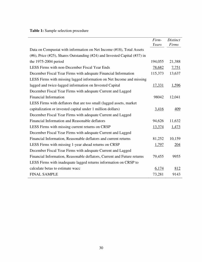
Table 1 outlines our sample selection procedure. We start with all firm-years on

Compustat in 1975-2004 with valid information on net income before extraordinary items

(#18), total assets (#6), price and shares outstanding at fiscal year end to compute market

capitalization (#24 and #25 respectively) and total invested capital (#37) needed to

compute residual income. We then restrict ourselves to only December fiscal year end

firms. We do this in order to ensure that our hedge strategies are not affected by timing

differences in the availability of fiscal year-end data. We lose a little over a third of our

potential sample, but ensure the integrity of our results. Our sample remains large and, as

later descriptive statistics will indicate, well spread out over industries and time. We need

to ensure that lagged information is available for earnings and lagged and twice-lagged

information is available for invested capital in order to compute current and lagged

residual income. Finally, we ensure that both contemporaneous as well as one-year ahead

information is available for the firms and that we have enough returns (at least 24 past

months) to compute cost of equity and wacc for all the firms in our sample. Our final

sample consists of 73,281 firm-years representing 9143 distinct firms, which averages

around 2443 firms per year on average.

15

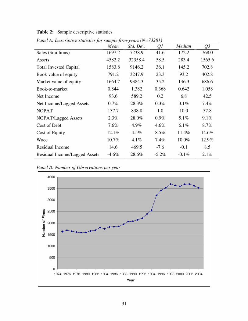
Table 2 presents descriptive statistics for the sample firms. The large differences

between means and medians for our size variables (sales, assets, total invested capital,

book and market value of equity) indicates the obvious skewness of these variables due to

the presence of large firms. There is also considerable variation in the book-to-market

ratio indicating that both value (high BM) and growth (low BM) stocks are potentially

present in the sample. We also present the unscaled and scaled (by lagged assets) values

of Net Income, NOPAT and Residual Income. Interestingly, while the median values of

Net Income and NOPAT are positive, the median residual income is barely negative,

indicating that less than half the firms in the sample cover their cost of capital.

Panel B of Table 2 graphically presents the number of observations per year. The

number of observations varies from a low of 1617 in 1978 to a high of 3698 in 2002. No

single year represents less than 2% or more than 5% of the sample, indicating that time

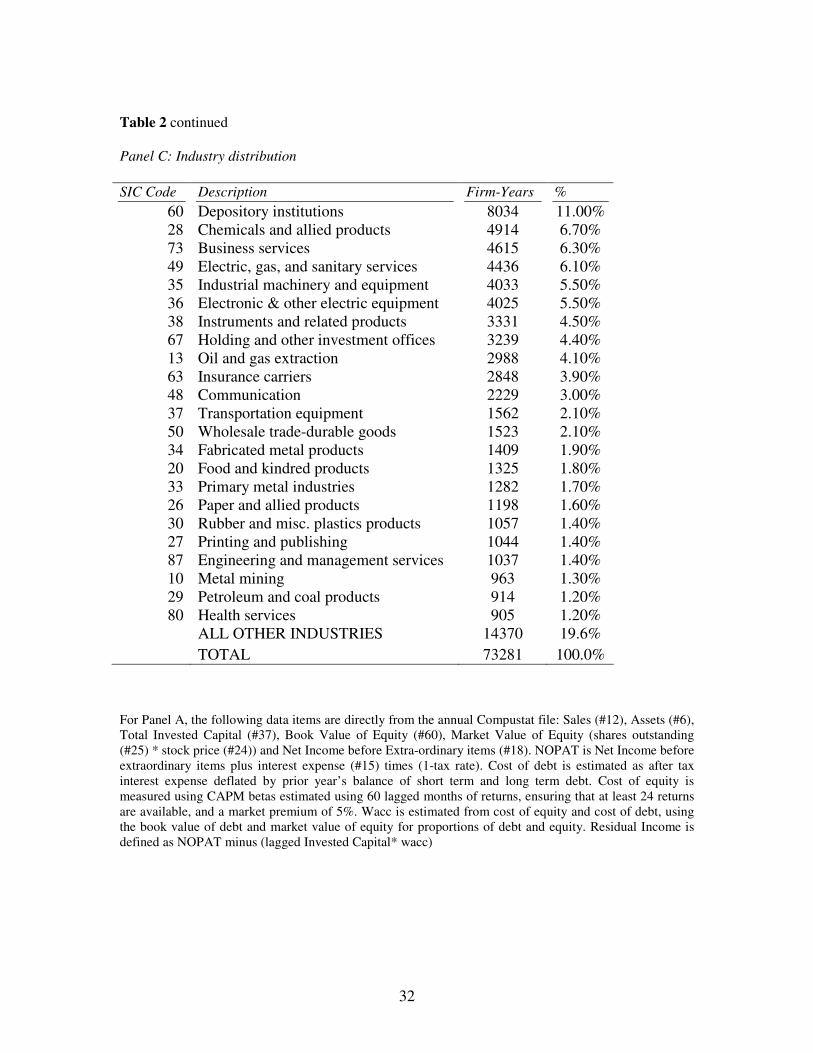
clustering is unlikely to be an issue. Panel C of Table 2 presents the industry distribution.

While no industry dominates our sample, the large number of depository institutions

(11%) and the small number of wholesale and retail firms (2-digit SIC codes from 50 to

59) may be related to our decision to focus on December fiscal year end firms.

Table 3 presents the descriptive statistics and correlations for the variables used in

our analysis. Our variables of interest are the changes in Net Income (∆NI) and Residual

Income (∆RI), both of which are scaled by lagged total assets. We are interested in their

relationship with contemporaneous market-adjusted returns (RETM0) and one-year-ahead

market-adjusted returns (RETM1). We also present the statistics for the scaled changes in

the capital charge component (∆CAPC) and interest component (∆INT) of residual

income.

16

Panel A presents the means of these variables. All variables with the exception of

return variables are winsorized at the 1% and 99% level using year-by-year distributions.4

By construction, the mean change in ∆RI (0.28%) equals the change in ∆NI (0.57%) plus

the change in the interest component (0.18%) minus the change in the capital charge

component (0.47%). The means of both contemporaneous as well as one-year ahead

returns are significantly greater than zero at around 5% as these are equally weighted

means while the market index used is the value weighted index; indeed the value

weighted means are close to zero.

Panel B presents the correlations between these variables. We present the means

of 30 year-by-year cross sectional correlations, both pearson as well as spearman rank-

order correlation. Not surprisingly, the changes in net income and residual income are

highly correlated (0.95 pearson, 0.86 spearman). This contrasts the much lower

correlation shown by BBW. We have two explanations for this. First –we rely on publicly

available data where the adjustments leading from NI to RI are very transparent and

clear. Second, we present the correlation between the changes in these variables, which

implies that the measurement errors in RI are likely to be mitigated by the differencing

process. Both ∆NI and ∆RI show strong correlation with current returns (RETM0); while

∆NI does show stronger correlation, ∆RI also shows almost the same correlation. Finally,

while both ∆NI and ∆RI show a weak correlation with future returns (RETM1), ∆RI

appears to have a slightly stronger correlation with future returns than ∆NI.

4 We do not winsorize the returns variables, as these variables are also used in our hedge portfolio returns analysis. As a sensitivity analysis, we delete outliers instead of winsorizing them. Results are very similar and not reported.

17

5. Results

5.1 Contemporaneous Return Regressions for Entire Sample

We first run return regressions for the entire sample. The dependent variable is

contemporaneous market-adjusted return. We use the 4 models specified in the research

design section. Consistent with prior research, we run pooled regressions over the 30 year

sample period. As a sensitivity test, we also run the regressions using year fixed-effects.

The results are very similar and not reported.5

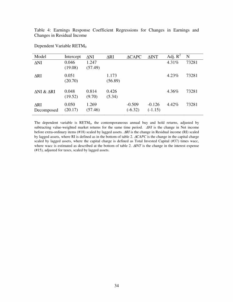
We present the results in Table 4. The first model uses the change in earnings

scaled by lagged assets (∆NI) as the dependent variable. As expected, ∆NI has a strong

correlation with current returns with a coefficient of 1.247 and a t-stat of 57.49. The

regression has an adjusted R2 of 4.31%. The second regression uses the change in

residual income instead of change in income. While the adjusted R2 does decline, it does

so only marginally to 4.23%. This contrasts with the results in BBW, who find a

significant decline when they move from NI to RI in their regressions.

In the next regression, we add both the change in Net Income and change in

Residual Income as independent variables, mindful of the high positive correlation

between these two measures, as is typical in these “horse-race” regressions. We find that

the change in Residual Income (∆RI) continues to be significant after the inclusion of net

income, and the explanatory power of the regression edges up to 4.36%.

Finally, we decompose change in residual income into the changes in the net

income, interest and capital charge components. As expected, we find that the change in

income component (∆NI) has a strong positive component and the change in the capital

5 Ideally, we would also like to run the tests at an annual level and report Fama-Macbeth (1973) style average coefficients. Unfortunately, the sample size is rather small in some of the partitions examined later on in some of the years, leading to unstable regression coefficients.

18

charge (∆CAPC) has a negative component. However the coefficient on ∆CAPC has a

smaller absolute magnitude than the coefficient on ∆NI. This can be viewed as

preliminary evidence that although the market does consider the capital charge in

contemporaneous returns, it does so only partially. This regression has the highest

explanatory power at 4.41%.

To summarize, we find that which residual income has a slightly smaller

association with returns than net income, the association is significant and incremental to

the association between returns and income. In future tests, we will view Net Income and

Residual Income not as competing metrics, but as complementary measures.

5.2 Contemporaneous Regressions based on Changes in Net Income and Residual

Income

We now focus on the basic ERC specification (equation 1) with contemporaneous

market adjusted returns as the dependent variable and change in Net Income (∆NI) as the

independent variable. We run this regression in the four different states of the world

based on whether changes in net income and residual income are positive or negative, i.e.

both decreasing (∆NI -, ∆RI -), NI decrease with an increase in RI (∆NI -, ∆RI +), NI

increase with a decrease in RI (∆NI +, ∆RI -), and finally both increasing (∆NI +, ∆RI +).

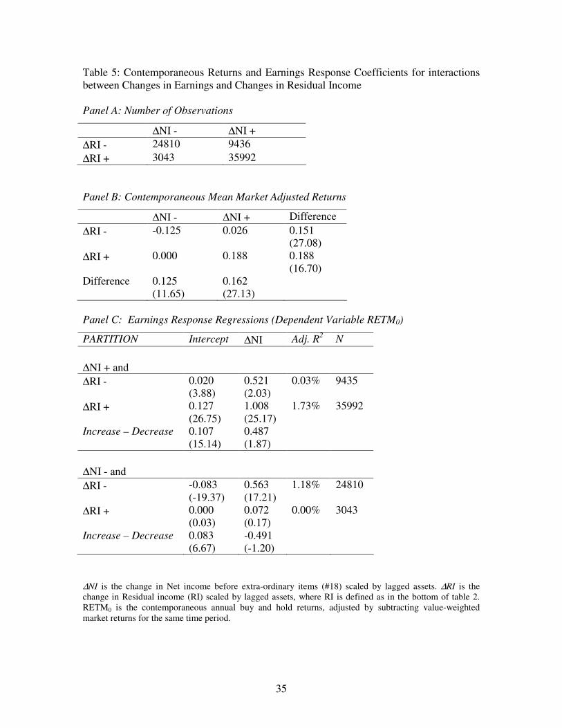
Panel A of Table 5 shows that changes in RI and Earnings typically move in the

same direction, as the measures move in the same direction in over 60,000 of the 73,281

observations, with 35992 observations of firms with increasing NI and RI and 24810

observations of firms with decreasing NI and RI.

However, concurrent movements in these measures are in different directions in

almost a fifth of the observations. The majority of these (9436) are in the case where

19

earnings increase, but residual income decreases. These are firms whose increase in

earnings is being achieved by additional investments that are not covering the

incremental cost of capital invested. If the market cares about investment efficiency, we

should see a smaller ERC for this group compared to the group where earnings and

residual income both increase.

In the smallest of the four groups, we see decreases in earnings while RI increases

(3043 observations). These are firms who are potentially divesting non-performing assets

in an effort to restore profitability. These actions, in turn, are likely to make earnings

(losses) even more transitory. We should expect these firms to have a lower ERC than

firms for which both NI and RI decrease.

Panel B of Table 5 displays the mean contemporaneous market adjusted returns

for each of the four above mentioned groups. Firms for which both RI and NI decline

earn the lowest market-adjusted returns at -12.5%, while firms with increases in both earn

the highest market-adjusted returns at +18.8%. Interestingly, firms for which earnings

decrease but residual income increases actually do not underperform the market. Finally,

firms which increase their earnings at the expense of lowered residual income earn small

positive excess returns (+2.6%). For both earnings increasing and earning decreasing

firms, the subgroup with increasing residual income is associated with higher returns.

We present these results merely as descriptive statistics. Indeed, the firms with

increasing residual income and decreasing net income may have higher returns simply

because their decline in net income is likely to have been less steep than firms where both

decline. Similarly, firms with increasing residual income and increasing net income may

also earn higher returns than firms with decreasing residual income and increasing net

20

income because their increase in net income is likely to have been greater. To formally

test the associations in these groups, we present the results from the ERC regressions.

Panel C of Table 5 presents the results of the regressions. We first consider the 2

partitions with increase in earnings. The ERC for the group with the increase in both NI

and RI at is significantly greater than the ERC for the subgroup with increase in NI and a

decline in RI (1.008 vs. 0.521). One way to interpret this is that the market capitalizes

positive changes in income at a lower rate when they are also not associated with positive

changes in residual income. Next, we consider the 2 partitions with a decline in earnings.

The ERC for the partition where NI declines but RI increases (0.072) is significantly

smaller than the partition for which both NI and RI decline (0.563). In other words, the

market is more likely to treat a loss as transitory when at least RI is increasing.

Hence the partitioned ERC regressions indicate that trends in residual income

provide information to help interpret changes in net income. Specifically, an increase in

net income is more likely to be viewed as good news when it is also associated with

increasing residual income, while a decline in net income is less likely to be viewed as

bad news when it is mitigated by increases in residual income. Our results are consistent

with findings in Harris and Nissim (2004), who show that earnings generated through

organic growth is valued at a higher rate than earnings acquired through investments.

5.3 Correlation with Future Returns

The evidence thus far indicates that residual income does add to the

informativeness of net income contemporaneously. However, it is also possible that the

market only partially impounds the information in residual income. If this is the case, we

should see a trend in future returns, as the information implicit in residual income trends

21

becomes apparent to the stock market. Specifically, we should expect firms with an

increase in residual income to earn positive future abnormal returns if the market only

partially capitalizes the good news implicit in increases in residual income, while

conversely, we should expect firms with a decline in residual income to earn negative

future abnormal returns.

In Panel A of Table 6, we present the mean market-adjusted 1-year-ahead returns

for the 4 partitions based on changes in net income and residual income. The first column

consists of firms with a decline in NI. Among these firms, firms with an increase in RI

earn significantly greater market adjusted returns than firms with a decline in RI. The

second column focuses on firms with an increase in NI. Here too the same pattern is

repeated, with firms that also see an increase in RI earning greater 1-year-ahead returns

than firms with a decline in RI. Interestingly, when we compare across columns, we find

that conditioning on trends in Net Income does not help separate firms in terms of their

future returns. Specifically, among firms with an increase (or decrease) in RI, there is an

insignificant difference between firms whose NI increased and those whose NI decreased.

One implication of this is that conditioning on residual income trends provides more

information regarding future returns.

Given that NI and RI are so closely linked, we focus on the one aspect that drives

the difference between the measures – the level of investment made to attain the income

level. We focus on the changes in invested capital used to determine the capital charge in

the computation of RI. As the results in Panel B of Table 6 indicate, firms with increasing

RI have substantially lower increase in invested capital as compared to firms with

decreasing RI. In both income-increasing as well as income-decreasing groups, the

22

difference in the change in invested capital is around 11-12%. For instance, amongst NI

increasers, the RI-increasing sub-group sees a change in invested capital of barely 0.8%,

while the RI-decreasing sub-group a substantial change in invested capital of 12.1%. The

differences in 1-year-ahead returns may have to do with the market realizing the

difference between income growth driven by increases in profitability as opposed to

income growth driven merely by increases in investment, again consistent with Harris

and Nissim (2004).

Panel C of Table 6 presents the market-adjusted 1-year-ahead returns for quintiles

based on changes in NI and changes in RI. The first set of columns present the results

based on changes in NI. One does see a positive correlation between changes in Net

Income and future returns. This is consistent with prior research on the post-earnings-

announcement drift (Bernard and Thomas 1989). The firms in the highest quintile of ∆NI

earn 2.7% more in terms of future returns than firms in the highest quintile of ∆NI.

However, the relationship is not monotonic, as firms in the middle quintile actually earn

the highest returns. In contrast, the difference in future returns between groups of firms in

the extreme quintiles of ∆RI is greater at 3.9%, and the relationship is strictly monotonic.

Hence, it appears that firms in the highest quintile of ∆RI systematically earn higher

returns in future periods.

The above results suggest that the market may not fully impound the implications

of changes in residual income and invested capital into price, suggesting the possibility of

generating hedge returns using these measures in a trading rule. However, it is also

possible that the return differences reported above may be clustered in certain time

periods and not consistent across time. To test whether the ability of ∆RI to generate

23

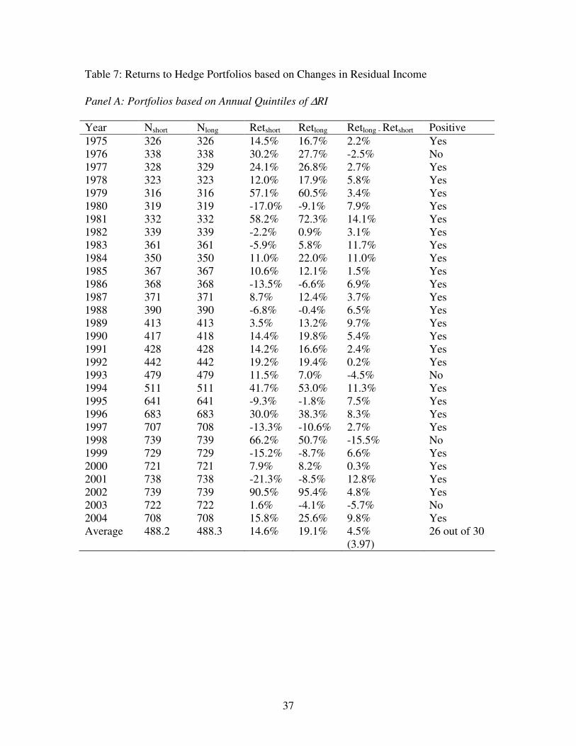
excess returns holds across time, we construct hedge portfolios in each year by going

long in firms in the top quintile of ∆RI and short in firms in the bottom quintile. The

results are reported in Panel A of Table 7. The average annual return to the hedge

portfolio is 4.5%, which is highly significant (t-stat=3.97). More importantly, the strategy

of going long in high ∆RI firms and short in low ∆RI firms generates positive returns in

26 out of the 30 years, indicating the robustness of the strategy as well as making it

unlikely that the higher risk could be contributing to the positive average returns. Figure

1 presents the results to the hedge strategy graphically. As the graph indicates, the

strategy earns returns below -5% in only one year, 1998. Interestingly, the future returns

for this year correspond to 1999, now acknowledged to be the peak year of the

technology bubble, when fundamentals played little or no role in stock returns.

When we replicate the strategy using ∆NI, the average return is only 2.5%, and

the strategy generates positive returns in only 20 out of 30 years (results not tabulated).

Comparing these results leads one to conclude that the returns to ∆RI are incremental to

any returns that may be associated with the post-earnings-announcement drift.

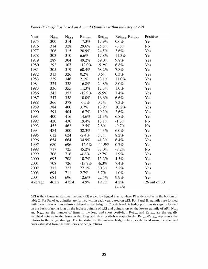
As a sensitivity test, we form quintiles based on changes in residual income

within industry (defined at the 2-digit SIC code level), and as before go long in the

highest ∆RI firms and short in the lowest ∆RI firms. The results are presented in Panel B

of Table 7. The results are very similar – the mean return is slightly lower at 4.2%, but

the t-stat actually increases marginally to 4.46. As before, the strategy generates excess

returns in most years (26 out of 30).

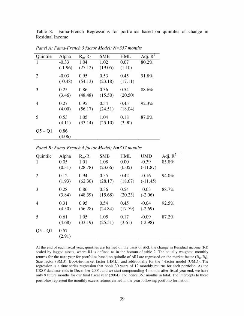
As a final test, we control for additional risk factors using the Fama-French

(1993) 3-factor and 4-factor models. We create calendar time portfolios of firms based on

24

the quintile of ∆RI. The 12 monthly returns to these portfolios in the year after portfolio

formation are regressed on the market factor (Rm-Rf), size factor (SMB), book-to-market

factor (HML) and additionally for the 4-factor model, momentum (UMD). While there is

debate about whether momentum is indeed a risk factor, we include it in our tests to

ensure that the results are incremental to a momentum effect, be it risk or mispricing.

This can also be viewed as a control for the post-earnings-announcement drift, which

potentially is a momentum effect. The regression is run in time series by pooling the

twelve future months for each of the thirty years. The intercept (alpha) of this regression

represents the average future monthly excess return for each quintile.

Panel A of Table 8 presents the results from the 3-factor model regression. Firms

in the lowest ∆RI quintile earn a significant negative return of -0.33%, while firms in the

highest ∆RI earn a significant positive return of 0.53%. The alphas also increase

monotonically from the lowest to the highest quintile. The difference between the alphas

of the extreme ∆RI portfolios is 0.86%, equivalent to an annualized difference of 10.8%.

Panel B of Table 8 presents the results to the 4-factor model. While the lowest

quintile firms no longer show a negative alpha, the monotonic relationship with quintile

of ∆RI continues to persist. The difference in alphas between the extreme quintiles is still

significant at 0.57%, equivalent to an annualized difference of 7.1%.

Taken together, Tables 6 through 8 show that the market does not fully

incorporate the implications of changes in residual income into contemporaneous price,

and that the extent of mispricing persists even after controlling for known risk factors.

This confounds interpretations of concurrent associations between returns and residual

income, commonly used in the prior literature to infer the “usefulness” of residual income

25

in contracting. Residual income attempts to capture efficiency in investment decisions,

the true value of which becomes apparent to the stock market only in the future.

5.4 Sensitivity Analyses

We conduct a number of sensitivity analyses to our base analysis. We use other

deflators to scale changes in net income and residual income such as lagged market value

and lagged invested capital. The results are essentially unchanged. We also recompute

residual income using a variety of different approaches including a flat 12% or 15% wacc

threshold for each firm as well as constant threshold for all firms in a given year, but

varying the threshold based on the changes in interest rates across time. We also calculate

residual income using Net Income, the cost of equity and lagged book values instead of

NOPAT, wacc and lagged invested capital. In all cases, our results and conclusions are

essentially unaltered. Finally, 11% of our sample consists of depository institutions for

which the conventional notions of investment may not be applicable. When we conduct

our analyses after excluding these firms, our results are generally unchanged and in some

instances even stronger.

6. Conclusion and Discussion:

This paper questions the results in prior research which indicate that residual

income has limited practical usefulness. Biddle, Bowen and Wallace (1997) and Chen &

Dodd (1997) find that residual income has only a minimally incremental association with

stock returns, relative to earnings.

This lack of association is puzzling given an extensive theoretical literature on the

usefulness of residual income and managing decentralized investment decisions, past

26

empirical evidence that that residual income based compensation is associated with

changes in investment, and historical arguments accountants have made in text books

from as early as the 1960’s.

In this paper, we posit three possible explanations for this puzzle. First, the

empirical literature may ignore some salient feature of practice or theory. Second, the

market does not fully impound all of the information from residual income into current

returns. Third, the theory abstracts away some relevant real world factors that limit the

applicability of residual income in practice. We test the first two explanations using a

research design motivated by insights regarding the cost of capital and hurdle rates found

in theory and in accounting texts.

Arguments in finance and accounting textbooks suggest that earnings might

increase simply based of incremental investments with returns that exceed the cost of

debt added to the firm. In contrast, since residual income requires a charge for the cost of

all capital employed, residual income may not increase even if earnings increase. Hence

changes in residual income combined with increases in earnings may be informative

about the nature of the earnings increase, and correspondingly the actions taken by

management. Accordingly, in this paper we examine changes in earnings and changes in

residual income in examining current stock returns, measures of investment and future

stock returns.

In our research design, we examine the associations among changes in residual

income, changes in earnings, and stock returns both concurrently and in the future.

Overall we find that conditional on whether residual income increased or decreased,

firms with increasing earnings exhibited systematic differences in invested capital,

27

contemporary returns, future returns, and the association between returns and earnings.

We interpret these results as consistent with residual income and earnings being jointly

informative of shareholder returns. In particular, changes in residual income facilitate

identifying the likelihood that earnings increases are the result of increasing investment

which does not cover the cost of capital employed. Our results suggest that such

investments dampen current returns and the contemporaneous association between

earnings and returns. Further our results suggest that contemporaneous returns do not

fully impound the implications of earnings which do not exceed the cost of capital, as

changes in current residual income predict future returns.

28

References

Anctil, R. 1996. Capital budgeting using residual income maximization. Review of

Accounting Studies 1, 9 – 50. Balachandran, S. 2006. How does residual income affect investment? The role of prior

performance measures. Management Science 52, 383-394. Baldenius, T., 2002. Delegated investment decisions and private benefits of control. The

Accounting Review 78, 909 – 930. Banker, R., and S. Datar. 1989. Sensitivity, Precision, and Linear Aggregation of

Accounting Signals. Journal of Accounting Research 27, 21-39. Bernard, V., and J. Thomas. 1989. Post-Earnings-Announcement Drift: Delayed Price

Response or Risk Premium? Journal of Accounting Research Supplement 27, 1-36.

Biddle, G., Bowen, R., and J. Wallace. 1997. Does EVA beat earnings? Evidence on the

associations with stock returns and firms values. Journal of Accounting and

Economics 24, 301-306. Chen, S., and J. Dodd. 1997. Economic Value Added (EVAtm): An empirical

examination of a new corporate performance measure. Journal of Management

Issues 9, 319-333. Dearden, J. 1972. How to make incentive plans work. Harvard Business Review 50,

117-122. Dutta, S., and S. Reichelstein. 2002. Controlling investment decisions: Depreciation and

Capital Charges. Review of Accounting Studies 7, 253 – 281. Fama, E., and K.French. 1993. Common Risk Factors in the Returns on Stocks and

Bonds. Journal of Financial Economics 33, 3-56. Fama, E., and J. MacBeth. 1973. Risk, Return and Equilibrium: Empirical tests. Journal

of Political Economy 81, 607-636. Garvey, G., and T. Millbroun, 2000. EVA versus earnings: does it matter which is more

highly correlated with stock returns? Journal of Accounting Research 38, 209-245.

Harris, T., D. Nissim, 2004. The Differential Value Implications of the Profitability and

Investment Components of Earnings. Working Paper - Columbia University.

29

Horngren, C., S. Datar, and G. Foster. 2006. Cost Accounting: A Managerial Emphasis. Prentice Hall, New Jersey.

Ittner, C. and D. Larcker. 2001. Assessing Empirical Research in Managerial Accounting:

A Value-Based Management Perspective. Journal of Accounting and Economics 32, 349-410.

Morse, D., and J. Zimmerman. 1997. Managerial Accounting, Richard D. Irwin, Chicago

IL. Reichelstein, S. 1997. Investment decisions and managerial performance evaluation.

Review of Accounting Studies 2, 157 – 180. Rogerson, W. 1997. Intertemporal cost allocation and management incentives: A theory

of explaining the use of economic value added as a performance measure.

Journal of Political Economy 105, 770-795. Simons, R. 2001. Vyaderm Pharmaceuticals. Harvard Business School Case # 9-101-

019. Harvard Business School Press. Solomons, D. 1965. Divisional Performance Measurement and Control. Richard D.

Irwin, Homewood, IL. Wallace, J. 1997. Adopting residual income based compensation, do you get what you

pay for? Journal of Accounting and Economics 24, 275 – 300.

30

Table 1: Sample selection procedure

Firm-

Years

Distinct

Firms

Data on Compustat with information on Net Income (#18), Total Assets

(#6), Price (#25), Shares Outstanding (#24) and Invested Capital (#37) in

the 1975-2004 period 194,055 21,388

LESS Firms with non-December Fiscal Year Ends 78,682 7,751

December Fiscal Year Firms with adequate Financial Information 115,373 13,637

LESS Firms with missing lagged information on Net Income and missing

lagged and twice-lagged information on Invested Capital 17,331 1,596

December Fiscal Year Firms with adequate Current and Lagged

Financial Information 98042 12,041

LESS Firms with deflators that are too small (lagged assets, market

capitalization or invested capital under 1 million dollars) 3,416 409

December Fiscal Year Firms with adequate Current and Lagged

Financial Information and Reasonable deflators 94,626 11,632

LESS Firms with missing current returns on CRSP 13,374 1,473

December Fiscal Year Firms with adequate Current and Lagged

Financial Information, Reasonable deflators and current returns 81,252 10,159

LESS Firms with missing 1-year ahead returns on CRSP 1,797 204

December Fiscal Year Firms with adequate Current and Lagged

Financial Information, Reasonable deflators, Current and Future returns 79,455 9955

LESS Firms with inadequate lagged returns information on CRSP to

calculate betas to estimate wacc 6,174 812

FINAL SAMPLE 73,281 9143

31

Table 2: Sample descriptive statistics

Panel A: Descriptive statistics for sample firm-years (N=73281)

Mean Std. Dev. Q1 Median Q3

Sales ($millions) 1697.2 7238.9 41.6 172.2 768.0

Assets 4582.2 32358.4 58.5 283.4 1565.6

Total Invested Capital 1583.8 9146.2 36.1 145.2 702.8

Book value of equity 791.2 3247.9 23.3 93.2 402.8

Market value of equity 1664.7 9384.3 35.2 146.3 686.6

Book-to-market 0.844 1.382 0.368 0.642 1.058

Net Income 93.6 589.2 0.2 6.8 42.5

Net Income/Lagged Assets 0.7% 28.3% 0.3% 3.1% 7.4%

NOPAT 137.7 838.8 1.0 10.0 57.8

NOPAT/Lagged Assets 2.3% 28.0% 0.9% 5.1% 9.1%

Cost of Debt 7.6% 4.9% 4.6% 6.1% 8.7%

Cost of Equity 12.1% 4.5% 8.5% 11.4% 14.6%

Wacc 10.7% 4.1% 7.4% 10.0% 12.9%

Residual Income 14.6 469.5 -7.6 -0.1 8.5

Residual Income/Lagged Assets -4.6% 28.6% -5.2% -0.1% 2.1%

Panel B: Number of Observations per year

0

500

1000

1500

2000

2500

3000

3500

4000

1974 1976 1978 1980 1982 1984 1986 1988 1990 1992 1994 1996 1998 2000 2002 2004

Year

Nu

mb

er o

f F

irm

s

32

Table 2 continued

Panel C: Industry distribution

SIC Code Description Firm-Years %

60 Depository institutions 8034 11.00% 28 Chemicals and allied products 4914 6.70% 73 Business services 4615 6.30% 49 Electric, gas, and sanitary services 4436 6.10% 35 Industrial machinery and equipment 4033 5.50% 36 Electronic & other electric equipment 4025 5.50% 38 Instruments and related products 3331 4.50% 67 Holding and other investment offices 3239 4.40% 13 Oil and gas extraction 2988 4.10% 63 Insurance carriers 2848 3.90% 48 Communication 2229 3.00% 37 Transportation equipment 1562 2.10% 50 Wholesale trade-durable goods 1523 2.10% 34 Fabricated metal products 1409 1.90% 20 Food and kindred products 1325 1.80% 33 Primary metal industries 1282 1.70% 26 Paper and allied products 1198 1.60% 30 Rubber and misc. plastics products 1057 1.40% 27 Printing and publishing 1044 1.40% 87 Engineering and management services 1037 1.40% 10 Metal mining 963 1.30% 29 Petroleum and coal products 914 1.20% 80 Health services 905 1.20%

ALL OTHER INDUSTRIES 14370 19.6%

TOTAL 73281 100.0% For Panel A, the following data items are directly from the annual Compustat file: Sales (#12), Assets (#6), Total Invested Capital (#37), Book Value of Equity (#60), Market Value of Equity (shares outstanding (#25) * stock price (#24)) and Net Income before Extra-ordinary items (#18). NOPAT is Net Income before extraordinary items plus interest expense (#15) times (1-tax rate). Cost of debt is estimated as after tax interest expense deflated by prior year’s balance of short term and long term debt. Cost of equity is measured using CAPM betas estimated using 60 lagged months of returns, ensuring that at least 24 returns are available, and a market premium of 5%. Wacc is estimated from cost of equity and cost of debt, using the book value of debt and market value of equity for proportions of debt and equity. Residual Income is defined as NOPAT minus (lagged Invested Capital* wacc)

33

Table 3: Descriptive Statistics for Analysis Variables. Panel A: Univariate Statistics (n= 73,281 observations)

Mean

Std.

Deviation

25th

percentile

Median

75th

percentile

∆NI 0.57% 11.00% -1.41% 0.34% 2.57% ∆RI 0.28% 11.78% -2.16% 0.11% 2.31% ∆CAPC 0.47% 3.04% -0.53% 0.22% 1.48% ∆INT 0.18% 1.48% -0.08% 0.00% 0.30% RETM0 5.33% 67.74% -26.98% -2.94% 23.32% RETM1 5.60% 64.16% -25.31% -1.91% 23.55%

Panel B: Time-series means of cross-sectional correlation coefficients

∆NI ∆RI ∆CAPC ∆INT RETM0 RETM1

∆NI 0.863 -0.041 -0.121 0.304 0.026 ∆RI 0.951 -0.360 -0.088 0.276 0.034 ∆CAPC -0.154 -0.406 0.268 -0.004 -0.034 ∆INT -0.138 -0.057 0.227 -0.089 -0.056 RETM0 0.246 0.228 -0.025 -0.045 0.076 RETM1 0.022 0.024 -0.030 -0.039 0.032

∆NI is the change in Net income before extra-ordinary items (#18) scaled by lagged assets. ∆RI is the change in Residual income (RI) scaled by lagged assets, where RI is defined as in the bottom of table 2.

∆CAPC is the change in the capital charge scaled by lagged assets, where the capital charge is defined as Total Invested Capital (#37) times wacc, where wacc is estimated as described at the bottom of table 2.

∆INT is the change in the interest expense (#15), adjusted for taxes, scaled by lagged assets. RETM0 and RETM1 respectively are contemporaneous and one-year-ahead annual buy and hold returns, adjusted by subtracting value-weighted market returns for the same time period.

34

Table 4: Earnings Response Coefficient Regressions for Changes in Earnings and Changes in Residual Income Dependent Variable RETM0

Model Intercept ∆NI ∆RI ∆CAPC ∆INT Adj. R2 N

∆NI 0.046 (19.08)

1.247 (57.49)

4.31% 73281

∆RI 0.051 (20.70)

1.173 (56.89)

4.23% 73281

∆NI & ∆RI 0.048 (19.52)

0.814 (9.70)

0.426 (5.34)

4.36% 73281

∆RI Decomposed

0.050 (20.17)

1.269 (57.46)

-0.509 (-6.32)

-0.126 (-1.15)

4.42% 73281

The dependent variable is RETM0, the contemporaneous annual buy and hold returns, adjusted by

subtracting value-weighted market returns for the same time period. ∆NI is the change in Net income

before extra-ordinary items (#18) scaled by lagged assets. ∆RI is the change in Residual income (RI) scaled

by lagged assets, where RI is defined as in the bottom of table 2. ∆CAPC is the change in the capital charge scaled by lagged assets, where the capital charge is defined as Total Invested Capital (#37) times wacc,

where wacc is estimated as described at the bottom of table 2. ∆INT is the change in the interest expense (#15), adjusted for taxes, scaled by lagged assets.

35

Table 5: Contemporaneous Returns and Earnings Response Coefficients for interactions between Changes in Earnings and Changes in Residual Income Panel A: Number of Observations

∆NI - ∆NI +

∆RI - 24810 9436

∆RI + 3043 35992

Panel B: Contemporaneous Mean Market Adjusted Returns

∆NI - ∆NI + Difference

∆RI - -0.125 0.026 0.151 (27.08)

∆RI + 0.000 0.188 0.188 (16.70)

Difference 0.125 (11.65)

0.162 (27.13)

Panel C: Earnings Response Regressions (Dependent Variable RETM0)

PARTITION Intercept ∆NI Adj. R2 N

∆NI + and

∆RI - 0.020 (3.88)

0.521 (2.03)

0.03% 9435

∆RI + 0.127 (26.75)

1.008 (25.17)

1.73% 35992

Increase – Decrease 0.107 (15.14)

0.487 (1.87)

∆NI - and

∆RI - -0.083 (-19.37)

0.563 (17.21)

1.18% 24810

∆RI + 0.000 (0.03)

0.072 (0.17)

0.00% 3043

Increase – Decrease 0.083 (6.67)

-0.491 (-1.20)

∆NI is the change in Net income before extra-ordinary items (#18) scaled by lagged assets. ∆RI is the change in Residual income (RI) scaled by lagged assets, where RI is defined as in the bottom of table 2. RETM0 is the contemporaneous annual buy and hold returns, adjusted by subtracting value-weighted market returns for the same time period.

36

Table 6: Future Returns by groups based on changes in Income and changes in Residual Income Panel A: 1 Year Ahead Mean Market Adjusted Returns

∆NI - ∆NI + Difference

∆RI - 4.3% 3.6% -0.6% (-0.93)

∆RI + 8.6% 6.8% -1.8% (-1.62)

Difference 4.3% (3.70)

3.1% (5.33)

Panel B: Changes in Invested Capital

∆NI - ∆NI + Difference

∆RI - 7.5% 12.1% 4.5% (23.97)

∆RI + -4.4% 0.8% 5.3% (16.08)

Difference -12.0% (-35.98)

-11.3% (-62.88)

Panel C: Future Returns based on Quintiles of ∆NI and ∆RI

Quintiles based on ∆NI Quintiles based on ∆RI Quintile N RETM1 Quintile N RETM1

1 14645 3.7% 1 14645 3.2% 2 14662 5.0% 2 14662 4.9% 3 14664 6.7% 3 14664 6.2% 4 14662 6.2% 4 14662 6.6% 5 14648 6.4% 5 14648 7.1%

Q5-Q1 2.7% Q5-Q1 3.9% (2.80) (4.12)

∆NI is the change in Net income before extra-ordinary items (#18) scaled by lagged assets. ∆RI is the change in Residual income (RI) scaled by lagged assets, where RI is defined as in the bottom of table 2. RETM1 is the one-year-ahead annual buy and hold returns, adjusted by subtracting value-weighted market

returns for the same time period. For Panel C, quintiles are formed within each year based on ∆NI and

∆RI.

37

Table 7: Returns to Hedge Portfolios based on Changes in Residual Income

Panel A: Portfolios based on Annual Quintiles of ∆RI

Year Nshort Nlong Retshort Retlong Retlong - Retshort Positive

1975 326 326 14.5% 16.7% 2.2% Yes 1976 338 338 30.2% 27.7% -2.5% No 1977 328 329 24.1% 26.8% 2.7% Yes 1978 323 323 12.0% 17.9% 5.8% Yes 1979 316 316 57.1% 60.5% 3.4% Yes 1980 319 319 -17.0% -9.1% 7.9% Yes 1981 332 332 58.2% 72.3% 14.1% Yes 1982 339 339 -2.2% 0.9% 3.1% Yes 1983 361 361 -5.9% 5.8% 11.7% Yes 1984 350 350 11.0% 22.0% 11.0% Yes 1985 367 367 10.6% 12.1% 1.5% Yes 1986 368 368 -13.5% -6.6% 6.9% Yes 1987 371 371 8.7% 12.4% 3.7% Yes 1988 390 390 -6.8% -0.4% 6.5% Yes 1989 413 413 3.5% 13.2% 9.7% Yes 1990 417 418 14.4% 19.8% 5.4% Yes 1991 428 428 14.2% 16.6% 2.4% Yes 1992 442 442 19.2% 19.4% 0.2% Yes 1993 479 479 11.5% 7.0% -4.5% No 1994 511 511 41.7% 53.0% 11.3% Yes 1995 641 641 -9.3% -1.8% 7.5% Yes 1996 683 683 30.0% 38.3% 8.3% Yes 1997 707 708 -13.3% -10.6% 2.7% Yes 1998 739 739 66.2% 50.7% -15.5% No 1999 729 729 -15.2% -8.7% 6.6% Yes 2000 721 721 7.9% 8.2% 0.3% Yes 2001 738 738 -21.3% -8.5% 12.8% Yes 2002 739 739 90.5% 95.4% 4.8% Yes 2003 722 722 1.6% -4.1% -5.7% No 2004 708 708 15.8% 25.6% 9.8% Yes Average 488.2 488.3 14.6% 19.1% 4.5%

(3.97) 26 out of 30

38

Panel B: Portfolios based on Annual Quintiles within industry of ∆RI

Year Nshort Nlong Retshort Retlong Retlong - Retshort Positive

1975 300 314 17.3% 17.9% 0.6% Yes 1976 314 328 29.6% 25.8% -3.8% No 1977 306 315 20.9% 24.5% 3.6% Yes 1978 303 310 6.6% 17.8% 11.3% Yes 1979 289 304 49.2% 59.0% 9.8% Yes 1980 292 307 -12.0% -5.2% 6.8% Yes 1981 305 319 60.4% 68.2% 7.8% Yes 1982 313 326 0.2% 0.6% 0.3% Yes 1983 339 346 2.1% 13.1% 11.0% Yes 1984 324 338 16.8% 24.8% 8.0% Yes 1985 336 355 11.3% 12.3% 1.0% Yes 1986 342 357 -12.9% -5.5% 7.4% Yes 1987 347 358 10.0% 16.6% 6.6% Yes 1988 366 378 -6.5% 0.7% 7.3% Yes 1989 384 400 3.7% 13.9% 10.2% Yes 1990 391 404 16.7% 19.3% 2.6% Yes 1991 400 416 14.6% 21.3% 6.8% Yes 1992 420 430 19.4% 18.1% -1.3% No 1993 453 463 12.5% 2.8% -9.7% No 1994 484 500 38.3% 44.3% 6.0% Yes 1995 612 624 -2.4% 5.8% 8.2% Yes 1996 654 664 34.9% 41.3% 6.4% Yes 1997 680 696 -12.6% -11.9% 0.7% Yes 1998 717 725 45.2% 37.0% -8.2% No 1999 706 716 -4.6% -2.7% 1.9% Yes 2000 693 708 10.7% 15.2% 4.5% Yes 2001 708 726 -13.7% -6.3% 7.4% Yes 2002 712 727 77.1% 80.3% 3.2% Yes 2003 694 711 2.7% 3.7% 1.0% Yes 2004 681 696 12.6% 22.5% 9.9% Yes Average 462.2 475.4 14.9% 19.2% 4.2%

(4.46) 26 out of 30

∆RI is the change in Residual income (RI) scaled by lagged assets, where RI is defined as in the bottom of

table 2. For Panel A, quintiles are formed within each year based on ∆RI. For Panel B, quintiles are formed within each year within industry defined at the 2-digit SIC code level. A hedge portfolio strategy is formed

on the basis of going long on the highest quintile of ∆RI and going short on the lowest quintile of ∆RI. Nlong and Nshort are the number of firms in the long and short portfolios. Retlong and Retshort are the equally weighted returns to the firms in the long and short portfolios respectively. Retlong-Retshort represents the returns to the hedge strategy. The t-statistic for the average hedge return is calculated using the standard error estimated from the time series of hedge returns

39

Table 8: Fama-French Regressions for portfolios based on quintiles of change in Residual Income Panel A: Fama-French 3 factor Model; N=357 months

Quintile Alpha Rm-Rf SMB HML Adj. R2

1 -0.33 1.04 1.02 0.07 80.2% (-1.96) (25.12) (19.05) (1.10)

2 -0.03 0.95 0.53 0.45 91.8% (-0.48) (54.13) (23.18) (17.11)

3 0.25 0.86 0.36 0.54 88.6% (3.46) (48.48) (15.50) (20.50)

4 0.27 0.95 0.54 0.45 92.3% (4.00) (56.17) (24.51) (18.04)

5 0.53 1.05 1.04 0.18 87.0% (4.11) (33.14) (25.10) (3.90)

Q5 – Q1 0.86 (4.06)

Panel B: Fama-French 4 factor Model; N=357 months

Quintile Alpha Rm-Rf SMB HML UMD Adj. R2

1 0.05 1.01 1.08 0.00 -0.39 85.8% (0.31) (28.78) (23.66) (0.05) (-11.87)

2 0.12 0.94 0.55 0.42 -0.16 94.0% (1.93) (62.30) (28.17) (18.67) (-11.45)

3 0.28 0.86 0.36 0.54 -0.03 88.7% (3.84) (48.39) (15.68) (20.23) (-2.06)

4 0.31 0.95 0.54 0.45 -0.04 92.5% (4.50) (56.28) (24.84) (17.79) (-2.69)

5 0.61 1.05 1.05 0.17 -0.09 87.2% (4.68) (33.19) (25.51) (3.61) (-2.98)

Q5 – Q1 0.57 (2.91)

At the end of each fiscal year, quintiles are formed on the basis of ∆RI, the change in Residual income (RI) scaled by lagged assets, where RI is defined as in the bottom of table 2. The equally weighted monthly

returns for the next year for portfolios based on quintile of ∆RI are regressed on the market factor (Rm-Rf), Size factor (SMB), Book-to-market factor (HML), and additionally for the 4-factor model (UMD). The regression is a time series regression that pools 30 years of 12 monthly returns for each portfolio. As the CRSP database ends in December 2005, and we start compounding 4 months after fiscal year end, we have only 9 future months for our final fiscal year (2004), and hence 357 months in total. The intercepts to these

portfolios represent the monthly excess returns earned in the year following portfolio formation.

40

Figure 1: Returns to Hedge Portfolios based on changes in Residual Income

-20.0%

-15.0%

-10.0%

-5.0%

0.0%

5.0%

10.0%

15.0%

20.0%

1975

1977

1979

1981

1983

1985

1987

1989

1991

1993

1995

1997

1999

2001

2003