Embed Size (px)
Citation preview
Iron Man
Zeiss LSM 510 Laser Scanning Confocal Microscope
User Guide
v. 1.4 (11/2016)
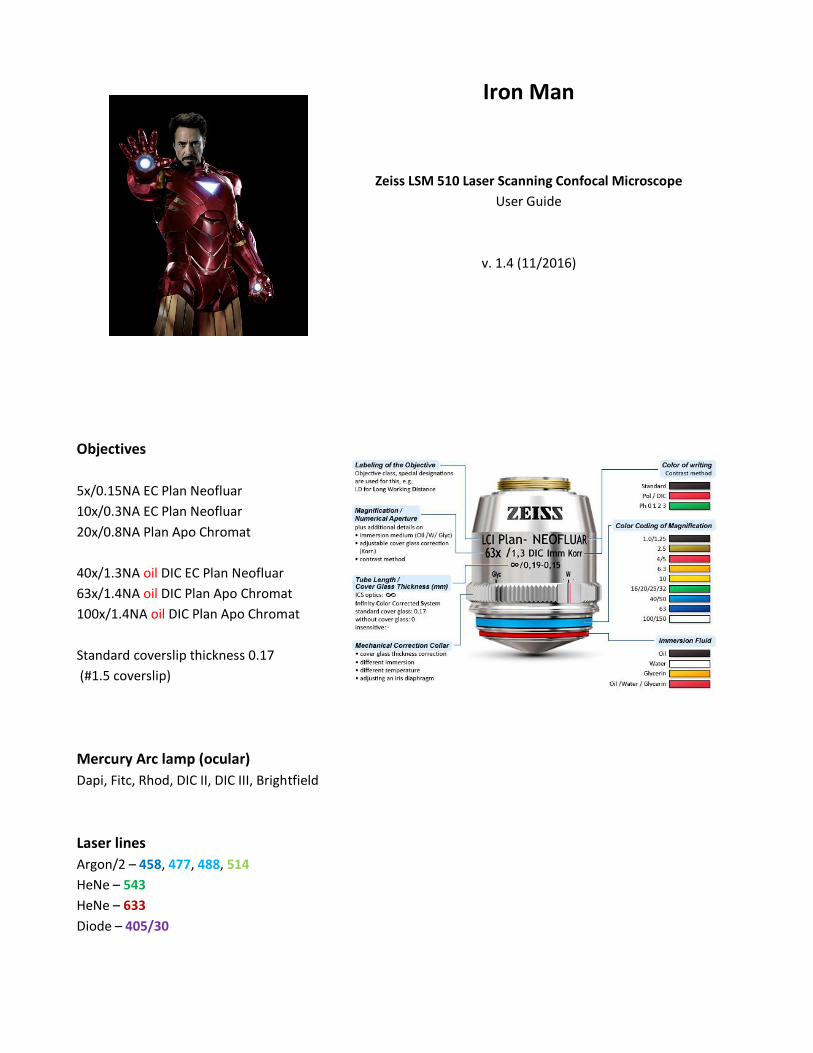
Objectives
5x/0.15NA EC Plan Neofluar
10x/0.3NA EC Plan Neofluar
20x/0.8NA Plan Apo Chromat
40x/1.3NA oil DIC EC Plan Neofluar
63x/1.4NA oil DIC Plan Apo Chromat
100x/1.4NA oil DIC Plan Apo Chromat
Standard coverslip thickness 0.17
(#1.5 coverslip)
Mercury Arc lamp (ocular)
Dapi, Fitc, Rhod, DIC II, DIC III, Brightfield
Laser lines
Argon/2 – 458, 477, 488, 514
HeNe – 543
HeNe – 633
Diode – 405/30
Iron Man User Guide v. 1.4 2
Contents:
Quick Guide 3
Starting up the system 4
The software will open to the ocular tab 5
To look at your slide 5
The Acquisition Tab 6
At the top
In the Setup Manager window
In the Imaging Setup window
In the Channels window
In the Online Acquisition window
Adjusting PMTs
Snap
Z series
The Information tab next to the image 11
When you’re done 11
APPENDIX A –Saving to your lab’s folder on MCDB Dept Server 12
APPENDIX B – Parts of the microscope 13
APPENDIX C – Configuring the Light Path 14

Iron Man User Guide v. 1.4 3
Quick Guide:
1) Turn on components in order. Don’t go too fast – PC & monitor won’t connect.
2) Log into Windows with IdentiKey and start Zen software.
3) Put sample on scope coverslip down. If using oil immersion, do not switch back to air
objective. No oil on air objectives!
4) Load or set up appropriate Channels/Tracks for imaging your sample.
5) Turn on necessary lasers. Do not turn on lasers you won’t be using. Argon/2 and Diode go to
Standby, then On. HeNe turn on. Argon/2: adjust % Output in Laser Properties window to
40% (do not go higher than 40%). Adjust once, then leave it alone.
6) Adjust imaging parameters – a. Laser attenuation % (3-5)
b. Frame size (512 x 512 or 1024x1024)
c. Scan Speed (~4-5 is good starting point, faster for live samples)
d. Averaging (1)
e. Zoom (1)
f. Pinhole (1 AU)
g. Offset (few to no blue understaturated pixels)
h. Gain (Master) (few to no red oversaturated pixels)
7) Snap for single frame image or set up parameters for Z-series or timelapse. Start Experiment.
8) Note the details in Information tab next to your image – these are useful to write in your
imaging notes.
9) Save and copy your data. The LMCF is not responsible for long-term data storage. See
Appendix A for information on how to transfer data to MCDB server.
10) Lower stage away from sample, and remove sample from stage. Properly clean oil off of any
immersion objectives you may have used with lens paper. If you are at all unsure of this
process, ask for help!
11) Leave the microscope on a low power objective for next user.
If someone is signed up within the next two hours (Check the MCDBCal!):
12) Switch lasers to Standby (if that option is available) or Off.
13) Close Zen.
14) Log use in Excel Sheet, save and close.
15) Log off Windows.
If no one is signed up within two hours or you are the last of the day:
13) Switch lasers to Standby, then Off.
14) Close Zen, confirming that lasers are all Off.
15) Log use in Excel Sheet, save and close.
16) Shut down system: Microscope base (#4), PC (#3, Start Shutdown), Mercury lamp (#2)
17) WAIT FOR THE FANS ON THE LASERS TO SLOW/COOL DOWN. This takes a couple minutes, and
the room should sound like it did when you walked in. Then flip the two switches (#1a & 1b).
Iron Man User Guide v. 1.4 4
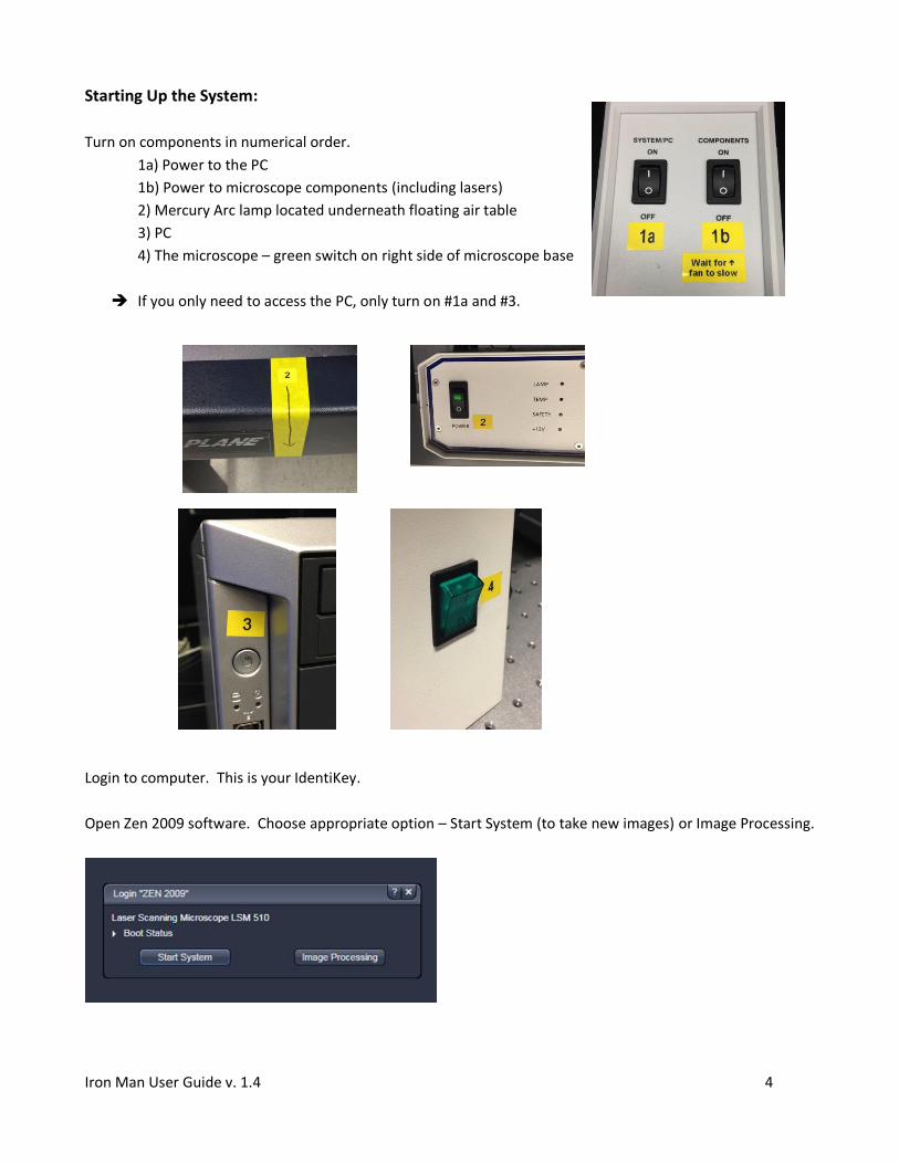
Starting Up the System:
Turn on components in numerical order.
1a) Power to the PC
1b) Power to microscope components (including lasers)
2) Mercury Arc lamp located underneath floating air table
3) PC
4) The microscope – green switch on right side of microscope base
If you only need to access the PC, only turn on #1a and #3.
Login to computer. This is your IdentiKey.
Open Zen 2009 software. Choose appropriate option – Start System (to take new images) or Image Processing.

Iron Man User Guide v. 1.4 5
The software will open to the ocular tab:
Online mode will allow you to view your sample through the oculars and offline mode allows you to view the
sample on the PC screen.
This window will allow you to control/view the following
microscope positions:
1) Halogen bulb for Brightfield viewing
2) Aperture
3) Specimen / stage
4) Objective – You can change the objective here or using
the buttons on the side of the microscope
USE CAUTION WHEN SWITCHING BETWEEN AIR AND
OIL OBJECTIVES
5) Reflector cubes – These should be changed using the
shortcut configurations above
6) Hg bulb shutter
7) Hg bulb
8) Lens
To minimize photobleaching of your sample, close the
Fluorescence Shutter whenever you are not looking
through the eyepieces.
To look at your slide:
1) Load the slide, coverslip down, onto the slide holders on the stage (these can be adjusted manually).
Please be sure that your slide is clean and dry – do not get wet mounting media or condensation on
the stage.
2) Position the slide over the desired objective.
- If you are using an air objective, start at the lowest focus position.
- If you are using oil immersion, place a small drop of oil on the slide before placing it on the
microscope. Do not switch back to an air objective. Turn the focus knob up until the objective
lens is just touching the oil.
3) Click into online mode, and choose the appropriate reflector cube configuration (#5) and open the
fluorescence shutter.
4) Looking through oculars, carefully focus on your sample and center on the structure you want to
image. Done? Close the fluorescence shutter and switch to offline mode.
2
3
4
5
5
8 6 7

Iron Man User Guide v. 1.4 6
The Acquisition Tab:
1) At the top – select any options you want for your
experiment (Z-series, time series)
2) In the Setup Manager window – turn on the appropriate
lasers for your experiment. You do not need to turn on
lasers you will not be using.
- Argon/2: Select Standby from dropdown to warm up the
laser. The status will read “Ready” when it is done.
Choose On. Open the Laser Properties window by
clicking on the arrow, and adjust laser output [%] to
40%. Do not go over 40% output or over 6.1 A. Do not
keep changing this Output % - set it for your imaging
session and leave it alone. Keeping the laser at 6.0 A is
done to assure that the laser output is at a stable and
reproducible intensity when using the confocal
scanhead.
- Diode: Select “Standby” from dropdown to warm up
the laser. The status will read “Ready” when it is
done, and only then can you choose “On”
- HeNe – choose “on” if you need these lasers
Iron Man User Guide v. 1.4 7
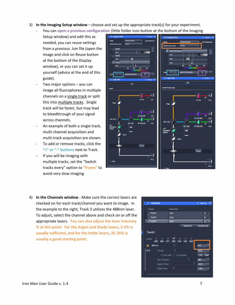
3) In the Imaging Setup window – choose and set up the appropriate track(s) for your experiment.
- You can open a previous configuration (little folder icon button at the bottom of the Imaging
Setup window) and edit this as
needed, you can reuse settings
from a previous .lsm file (open the
image and click on Reuse button
at the bottom of the Display
window), or you can set it up
yourself (advice at the end of this
guide).
- Two major options – you can
image all fluorophores in multiple
channels on a single track or split
this into multiple tracks. Single
track will be faster, but may lead
to bleedthrough of your signal
across channels.
- An example of both a single track,
multi-channel acquisition and
multi-track acquisition are shown.
- To add or remove tracks, click the
“+” or “-“ buttons next to Track.
- If you will be imaging with
multiple tracks, set the “Switch
tracks every” option to “frame” to
avoid very slow imaging
4) In the Channels window - Make sure the correct lasers are
checked on for each track/channel you want to image. In
the example to the right, Track 3 utilizes the 488nm laser.
To adjust, select the channel above and check on or off the
appropriate lasers. You can also adjust the laser intensity
% at this point. For the Argon and Diode lasers, 3-5% is
usually sufficient, and for the HeNe lasers, 25-35% is
usually a good starting point.
Iron Man User Guide v. 1.4 8
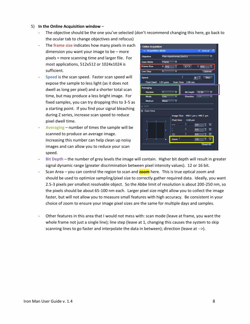
5) In the Online Acquisition window –
- The objective should be the one you’ve selected (don’t recommend changing this here, go back to
the ocular tab to change objectives and refocus)
- The frame size indicates how many pixels in each
dimension you want your image to be – more
pixels = more scanning time and larger file. For
most applications, 512x512 or 1024x1024 is
sufficient.
- Speed is the scan speed. Faster scan speed will
expose the sample to less light (as it does not
dwell as long per pixel) and a shorter total scan
time, but may produce a less bright image. For
fixed samples, you can try dropping this to 3-5 as
a starting point. If you find your signal bleaching
during Z series, increase scan speed to reduce
pixel dwell time.
- Averaging – number of times the sample will be
scanned to produce an average image.
Increasing this number can help clean up noisy
images and can allow you to reduce your scan
speed.
- Bit Depth – the number of grey levels the image will contain. Higher bit depth will result in greater
signal dynamic range (greater discrimination between pixel intensity values). 12 or 16 bit.
- Scan Area – you can control the region to scan and zoom here. This is true optical zoom and
should be used to optimize sampling/pixel size to correctly gather required data. Ideally, you want
2.5-3 pixels per smallest resolvable object. So the Abbe limit of resolution is about 200-250 nm, so
the pixels should be about 65-100 nm each. Larger pixel size might allow you to collect the image
faster, but will not allow you to measure small features with high accuracy. Be consistent in your
choice of zoom to ensure your image pixel sizes are the same for multiple days and samples.
- Other features in this area that I would not mess with: scan mode (leave at frame, you want the
whole frame not just a single line); line step (leave at 1, changing this causes the system to skip
scanning lines to go faster and interpolate the data in between); direction (leave at -->).

Iron Man User Guide v. 1.4 9
6) Adjusting PMTs
These guidelines assume a fixed sample. For live samples, you should try to avoid Auto Expose or
Continuous modes as these will expose your sample to large amounts of excitation light prior to image
acquisition. Instead use Live mode or optimize in one region of slide
and move to another for data acquisition.
This step depends on your experimental design and question. To
ensure that your images are quantitative, you must avoid over- or
understaurating pixels, as you will not be able to properly measure
intensity in this case. It is also important to remember that your
brightest sample may be a particular Z plane, later slide, alternate
timepoint, and these may be oversaturated when you get to them
later.
- Select the first channel to optimize (check on/off in Imaging
Setup area). I usually prefer to optimize one channel/track
at a time, but if you plan to use multiple lasers on a single
track, make sure these will all be on during optimization.
- Ensure that your sample is on the brightest Z plane – go to
live mode and adjust using focus knob.
- Set lasers to appropriate starting values - for the Argon
and Diode lasers, 3-5% is usually sufficient, and for the
HeNe lasers, 25-35% is usually a good starting point.
- Set the pinhole size to 1AU. Unless you have a deliberate
reason to change this, 1AU is good for most experiments.
(Bigger pinhole = more light = less “confocal”). Don’t go
smaller. Bigger is useful for if you need to image a really
thick sample and do not want to image many 1AU confocal
slices.
- Click Auto Expose. The software will now attempt to set
the gain and offset for that channel.
- Click Continuous, and select the Range indicator Look Up
table beneath the image. Oversaturated pixels will appear
red and undersaturated pixels will appear blue. You can
manually adjust the gain and offset to achieve a good
balance between over- and undersaturation for your
experiment. You should adjust the offset first. This will
adjust the background. Be aware that if you change this too much you
will also remove signal form your sample. A little goes a LONG way, go
down to add undersaturated pixels, go up if you have too many
undersaturated pixels. After adjusting the offset, adjust the gain
(master). This will adjust the foreground and background signals. If you
are at the high end of gain, bump up laser power; if you are at low end,
reduce laser power.
- Repeat these steps for all channels in your experiment.

Iron Man User Guide v. 1.4 10
7) Snap – If you just want a single plane, click snap and save your
image. The PC does not have a lot of RAM – save and close
regularly.
8) Z series – If you selected Z-stack in the top left, you can now
control the Multidimensional Acquisition Z-stack window. You
can choose to either set the first and last positions, or you can
choose to center the stack around a given position.
- First/Last ( most common choice)
o Click Live
o Turn focus knob on microscope in one
direction until desired distance is
reached, click set last
o Repeat in the other direction, click set
first
o Either choose number of slices or step
size. The software will suggest the
optimal step size. This is for Nyquist
sampling - ~2 Z planes per confocal
volume, depends on pinhole size and
wavelengths being used.
- Center
o Click Live
o Turn focus knob to get to center plane
of sample
o Either choose number of slices or step
size. The software will suggest the
optimal step size.
o Click Range Select.
o Move green line to approximate center of sample and red
lines to desired top and bottom of sample.
- Click Start Experiment. Time remaining will be shown at the
bottom of the screen.
- Save results.
Iron Man User Guide v. 1.4 11
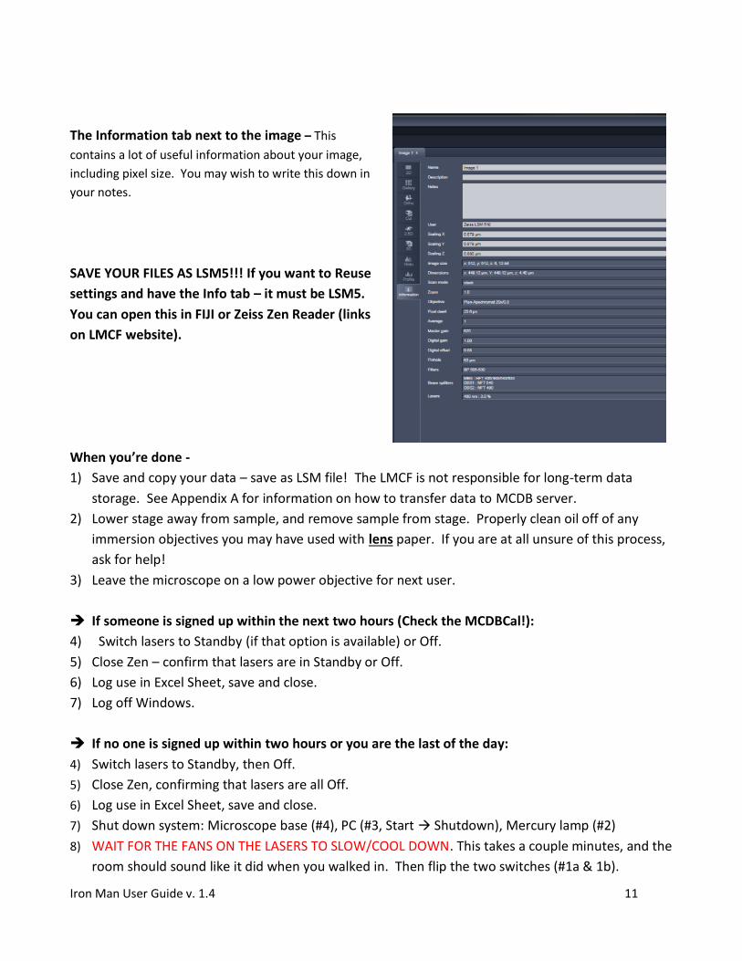
The Information tab next to the image – This
contains a lot of useful information about your image,
including pixel size. You may wish to write this down in
your notes.
SAVE YOUR FILES AS LSM5!!! If you want to Reuse
settings and have the Info tab – it must be LSM5.
You can open this in FIJI or Zeiss Zen Reader (links
on LMCF website).
When you’re done -
1) Save and copy your data – save as LSM file! The LMCF is not responsible for long-term data
storage. See Appendix A for information on how to transfer data to MCDB server.
2) Lower stage away from sample, and remove sample from stage. Properly clean oil off of any
immersion objectives you may have used with lens paper. If you are at all unsure of this process,
ask for help!
3) Leave the microscope on a low power objective for next user.
If someone is signed up within the next two hours (Check the MCDBCal!):
4) Switch lasers to Standby (if that option is available) or Off.
5) Close Zen – confirm that lasers are in Standby or Off.
6) Log use in Excel Sheet, save and close.
7) Log off Windows.
If no one is signed up within two hours or you are the last of the day:
4) Switch lasers to Standby, then Off.
5) Close Zen, confirming that lasers are all Off.
6) Log use in Excel Sheet, save and close.
7) Shut down system: Microscope base (#4), PC (#3, Start Shutdown), Mercury lamp (#2)
8) WAIT FOR THE FANS ON THE LASERS TO SLOW/COOL DOWN. This takes a couple minutes, and the
room should sound like it did when you walked in. Then flip the two switches (#1a & 1b).

Iron Man User Guide v. 1.4 12
APPENDIX A – Saving to your lab’s folder on Collie (MCDB Dept Server):
Questions regarding MCDB Server should be directed to Erik Hedl.
1) Map the network drive. Right click on Computer icon on desktop or Computer in Start menu.
Click on “Map network drive…”
2) Drive letter should be Z: and the folder should be \\collie.int.colorado.edu\<your lab name>
(for example \\collie.int.colorado.edu\OlwinLab).
If your login for Collie is not your IdentiKey, check the box “connect using different
credentials.”
3) Click finish.
4) If you selected “connect using different credentials,” enter your username and password.
5) Click Ok and the drive should now appear. Copy over your files. If you have a lot of files, be
sure to allow time for the transfer. Under ideal conditions you will be able to copy close to 42
gigabytes per hour, don’t count on ideal conditions. Also, it is safer to copy (not move) your
files, then delete after the copy has completed.
You cannot, must not, should not reserve time on the microscopes in MCDB Cal to copy data –
reservations are for imaging only.
The LMCF PCs are not long-term data storage places and we are not responsible for lost data.
Do not forget to always safely store and backup your raw data – this represents the ground
truth of what you acquired that day and has all the associated metadata. Many journals are
now requiring that you submit raw data with your manuscript.
Iron Man User Guide v. 1.4 13
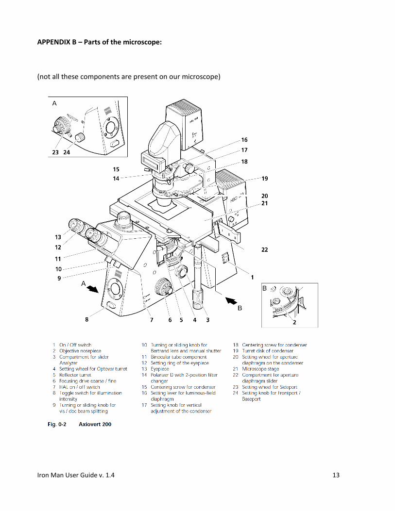
APPENDIX B – Parts of the microscope:
(not all these components are present on our microscope)

Iron Man User Guide v. 1.4 14
APPENDIX C – Configuring the Light Path:
Only turn on lasers you actually need
To turn on Argon/2 and Diode, first go to Standby and when it
says Ready, then turn it on. Argon/2 output [%] should be 50%
(do not go higher).
If you have multiple colors, you need to choose if you will
be imaging all channels in a single track or each channel in a
separate track (multi-track).
Single track is faster but can lead to bleedthrough of signal.
You can do a combination of multi-track and multi-channel –
for example, image DAPI and red together in a mult-channel
track and image green separately in its own track.
Load a premade track by clicking on the folder icon. If you
will be using the same track configuration many times, you
can save it here. Note: the loading and saving is done per
track.
This is where you can configure the mirrors and filters in
the light path and check off which channels to image per
track.
Let’s go through an example for imaging a triple labelled
sample (DAPI, FITC, Rhodamine) in a single track and
multitrack configuration.

Iron Man User Guide v. 1.4 15
- You need to know the excitation and emission spectra for all the dyes/fluorophores/probes you
will be using. This can readily be viewed in various Spectrum viewers on the web (list of which is on
the LMCF Website Resources tab at the bottom. Life Technologies’ SpectraViewer is a
straighforward and reasonably complete one. Excitation spectra are shown as dotted lines and
emission spectra are solid
- Next, figure out which lasers are appropriate. Available lines: Argon/2 – 458, 477, 488, 514; HeNe
– 543; HeNe – 633; Diode – 405/30. In this example, we’ll use the 405 (DAPI), 488 (FITC) and 543
(Rhodamine). Shown here are the excitation spectra and the laser lines we’ve selected.

Iron Man User Guide v. 1.4 16
- Now we need to configure the mirrors and filters appropriately. In the light path window, you
can click on the different positions to see what available options exist in this microscope. The laser
button is self-explanatory. From there, the light goes through a (1) dichroic (which will reflect or
transmit certain wavelengths only), then to your (2) sample, back up through the (1) dichroic,
through (3, 4) additional dichroics to separate out the different wavelengths, and through (5, 6, 7)
emission filters based on your sample.
- Available choices for each position:
(1) Dichroic (labeled based on what wavelengths it reflects; it should reflect the laser down to
the sample and transmit the emission from the sample through) – 405/488, 405/514/594,
405/488/543/633, 458, 458/514, 488/543, 488/594, NFT 80/20 (neutral density filter,
passes 80% and blocks 20%)
(2) <Sample>
(3) Dichroic (split emission signal from multiple fluorphores, labelled based on what
wavelengths it reflects) – none, plate, mirror, >515, >545, >595, >635 VIS, <545
(4) Dichroic (split emission signal from multiple fluorphores, labelled based on what
wavelengths it reflects) – mirror, >490, >515, >545
(5) Emission filter (labelled based on what it allows through; LP means long pass and it will
allow to pass anything greater than the given wavelength; BP means band pass and it will
allow to pass anything between the given wavelengths) – LP505, LP560, LP615, LP650,
BP505-530, BP505-550, BP530-560, BP560-615
(6) Emission filter – LP420, LP475, LP505, BP420-480, BP470-500, BP505-530, BP505-570IR
(7) Emission filter – LP420, LP475, LP505, LP530, LP560, LP615, LP650
Iron Man User Guide v. 1.4 17
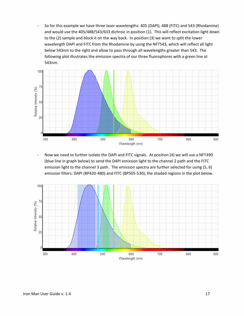
- So for this example we have three laser wavelengths: 405 (DAPI), 488 (FITC) and 543 (Rhodamine)
and would use the 405/488/543/633 dichroic in position (1). This will reflect excitation light down
to the (2) sample and block it on the way back. In position (3) we want to split the lower
wavelength DAPI and FITC from the Rhodamine by using the NFT543, which will reflect all light
below 543nm to the right and allow to pass through all wavelengths greater than 543. The
following plot illustrates the emission spectra of our three fluorophores with a green line at
543nm.
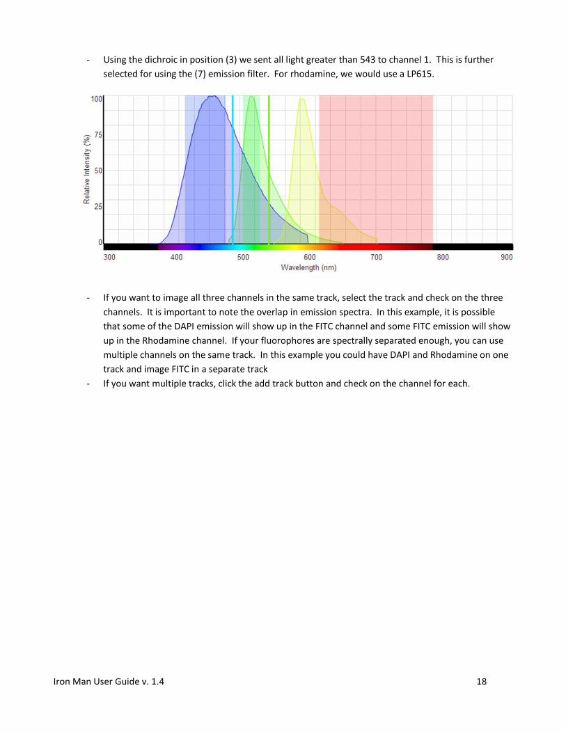
- Now we need to further isolate the DAPI and FITC signals. At position (4) we will use a NFT490
(blue line in graph below) to send the DAPI emission light to the channel 2 path and the FITC
emission light to the channel 3 path. The emission spectra are further selected for using (5, 6)
emission filters: DAPI (BP420-480) and FITC (BP505-530); the shaded regions in the plot below.
Iron Man User Guide v. 1.4 18
- Using the dichroic in position (3) we sent all light greater than 543 to channel 1. This is further
selected for using the (7) emission filter. For rhodamine, we would use a LP615.
- If you want to image all three channels in the same track, select the track and check on the three
channels. It is important to note the overlap in emission spectra. In this example, it is possible
that some of the DAPI emission will show up in the FITC channel and some FITC emission will show
up in the Rhodamine channel. If your fluorophores are spectrally separated enough, you can use
multiple channels on the same track. In this example you could have DAPI and Rhodamine on one
track and image FITC in a separate track
- If you want multiple tracks, click the add track button and check on the channel for each.


![Iron man protocal [thaicomix]](https://img.dokumen.tips/doc/110x75/558b5495d8b42a42698b458b/iron-man-protocal-thaicomix.jpg)