Investment performance of shorted leveraged ETF pairs Xinxin Jianga and Stanley Peterburgskyb,*

aSuffolk University, 73 Tremont Street, Boston, MA 02108

bKean University, 1000 Morris Avenue, Union, NJ 07083 *Corresponding author. E-mail: phinance@hotmail.com Abstract We analyze trading strategies involving triple-leveraged and inverse triple-leveraged ETF pairs by simulating daily returns over a 48 year period. Our results show that many such strategies significantly outperform the S&P 500 on a risk-adjusted basis. The Sharpe ratio appears to be maximized when shorting the bear triple-leveraged ETF and the bull triple-leveraged ETF in a 2:1 proportion, and simultaneously holding Treasuries long. In this case we find that the average annual Sharpe ratio is more than four times higher than for the S&P 500, and that the strategy outperforms the market in 43 of the 48 years. JEL classification: G11, G17 Keywords: exchange traded funds, ETFs, pair trading, portfolio management

This version: 1/13/13

2

I. Introduction

Leveraged and inverse leveraged exchange traded funds (ETFs) have seen tremendous

growth in popularity among investors since their introduction to financial markets in 2006. These

instruments attempt to deliver specific multiples of the return on an underlying index, such as the

S&P 500, on (usually) a daily basis. For example, the triple-leveraged ETF ProShares UltraPro

S&P 500 (UPRO) seeks daily investment results corresponding to triple the daily performance of

the S&P 500, while the inverse triple-leveraged ETF ProShares UltraPro Short S&P 500 (SPXU)

seeks daily investment results corresponding to triple the inverse (i.e., negative) of the daily

performance of the S&P 500. To accomplish these investment objectives, leveraged and inverse

leveraged ETFs enter into futures and/or swap contracts tied to the underlying index.1

It is well established that, although leveraged and inverse leveraged exchange traded

funds (henceforth, collectively, LEFTs) come close to achieving their target performance on a

daily basis, long-run LETF returns generally do not equal the target leverage times the index

returns (see, for example, Avellaneda and Zhang (2009), Cheng and Madhavan (2009),

Lauricella (2009), Jarrow (2010), Charupat and Miu (2011), and Tang and Xu (2012)) because of

the so-called constant leverage trap. In particular, both leveraged ETFs and inverse leveraged

ETFs linked to the same underlying index often underperform the index, and by a large margin,

over periods measured in months or years. Consider, for example, the performance of UPRO and

SPXU during the one-week period 4/1/10 - 4/7/10 and the eighteen-month period 4/1/10 -

10/1/11. Figure 1 shows that in the short run UPRO achieved a return approximately equal to 3×

In order to

keep the target leverage constant, the funds adjust their exposure to the index by rebalancing

their futures and/or swap holdings on a daily basis.

1 The details of the process involved in constructing leveraged and inverse leveraged positions are described in http://www.proshares.com/media/documents/components_of_leveraged_and_inverse_funds.pdf

3

that of the S&P 500, while SPXU attained a return close to -3× that of the S&P 500. However, in

the long run both funds underperformed the index by more than 15%. Cheng and Madhavan

(2009) illustrate similar underperformance for ProShares UltraShort Oil & Gas (DUG) and

ProShares Ultra Oil & Gas (DIG), which are tied to the Dow Jones U.S. Oil & Gas Index with

target leverage of -2× and 2×, respectively.

Our goal is to shed light on whether trading strategies involving LETF pairs have the

potential to outperform the S&P 500. In particular, if the poor performance of UPRO and SPXU

over long periods of time discussed above is typical, it may be possible to short both funds and

generate profits higher than those offered by the index. It should be noted that the shorting

strategy is not without risk. At times, one of the paired LETFs may significantly outperform the

index (when held long) over an extended time period, resulting in poor pairs trade performance.

For example, Figure 2 shows that during 11/21/2011 - 4/2/2012, a 50%-50% allocation to UPRO

and SPXU would have produced a positive return, and therefore a shorting strategy with the

same weights would have produced a negative return. On the other hand, the S&P enjoyed a

return of about 18% – much better than the shorting strategy. Ultimately, whether a shorting

strategy can be relied upon to consistently outperform the S&P is an empirical question. Since

LETFs are relatively new products with short track records, we attempt to answer this question

by simulating LETF returns.

Our research would be of only theoretical significance if it were difficult or impossible to

borrow shares of LETFs, since shorting requires a simultaneous borrowing and selling of the

security in question. As it turns out, many, if not most, LETFs can be shorted in practice. In fact,

one of the authors of this paper has been shorting LETFs in his modestly sized online brokerage

account for some time. Occasionally, the brokerage firm requests that the short position be

4

partially or fully closed out, but such requests are infrequent. Anecdotal evidence suggests that

the size of the account does play a role in determining the likelihood of it being targeted by the

brokerage when shares need to be returned to a lender.

We focus specifically on UPRO and SPXU because they are very liquid funds, with

average holding periods of less than 2 days and less than 3 days, respectively, and average bid-

ask spreads of only 0.04% and 0.03%, respectively, and because the underlying index is the

broad U.S. stock market. Other triple-leveraged and inverse triple-leveraged ETFs are somewhat

less liquid and/or track either a subset of the U.S. stock market or other financial or real asset

markets. In addition, UPRO and SPXU shares can be, and have been, sold short.

The rest of this article is organized as follows. In Section II we review prior literature. In

Section III, we describe our simulation design. In Section IV, we present our main findings on

the long-term performance of various shorted leveraged ETF pairs strategies. In Section V, we

discuss the affect of dividends, tracking errors, transaction costs, fund fees and expenses, and

taxes on the performance of these strategies. Finally, we summarize our research and offer

concluding remarks in Section VI.

II. Literature review

Leveraged ETFs are a recent financial innovation, and the research in this area is still in

its infancy. To our knowledge, this paper is the first to examine shorting strategies using LETFs.

Other studies of LETFs have focused on modeling the return dynamics, examining the sources

and characteristics of tracking errors, investigating the effect of LETF trading on underlying

security trading, and discussing the suitability of LETFs for retail investors.

5

Wang (2009), Avellaneda and Zhang (2009), and Cheng and Madhavan (2009) model the

stochastic process of LETF returns where the underlying index return process is assumed to

evolve as a geometric Brownian motion. They show that if the prices of an LETF and the index

are given by tA and tS , respectively, then, assuming t

t

dStS dt dWµ σ= + , the price of the index at

time T is 2( /2)0

T T zTS S e µ σ σ− += , while the price of the LETF at time T is 2 2( /2)

0T T z

TA A e λµ λ σ λσ− += ,

where z is a standard normal random variable and λ is the target leverage. It can be shown that

the relationship between the index return and the LETF return is ( ) 2 2

0 0

( ) /2T TA S TA S e

λλ λ σ−= . The upshot

is that since 2( )λ λ− is negative for any leveraged or inverse leverage ETF, the scalar term

2 2( ) /2Te λ λ σ− is less than 1, and therefore the LETF return is less than the compounded index return.

Hence, assuming index returns follow a geometric Browning motion, the LETF will lose money

unless index performance is sufficiently strong.

Charupat and Miu (2011) examine a group of Canadian LETFs, and report that they have

extremely small daily tracking errors. However, they define tracking errors in terms of net asset

values (NAV) rather than LETF prices. Whether daily LETF returns are close to their targets

remains unanswered. Tang and Xu (2012) find that daily tracking errors for a set of LETFs

linked to the S&P 500, Dow Jones, and NASDAQ-100, are substantial. LETF managers

consistently underleverage, and the effect on fund performance accumulates over time. The main

cause of this underexposure appears to be the cost of adjusting exposure on a daily basis. Shum

and Kang (2012) report that daily tracking errors for a set of LETFs linked to the Toronto Stock

Exchange, gold, oil & gas, MSCI EAFE, and the S&P 500 are sizeable as well. Once again,

underexposure to the underlying index appears to be the main source of deviation from target

returns.

6

Cheng and Madhavan (2009) investigate the effect of LETFs on market volatility. They

show that the required daily re-leveraging around the market close imparts additional systemic

risk to the market. This phenomenon is expected to become more pronounced as aggregate LETF

assets under management continue to increase. The debate as to whether LETFs are partly

responsible for the recent increase in market volatility has been picked up by the media (Sorkin

(2011), Kephart (2012)). Haryanto, et al. (2012) find that although LETF rebalancing demands

do lead to higher market volatility, this effect is economically significant only when the market

experiences a large positive or negative return by 3:30 PM. Bai, et al. (2012) examine whether

two real estate-linked and four financials-linked LETFs influence the late-day volatility of 63

real estate sector stocks, and report greatest impacts for smaller, less actively traded, and more

volatile stocks.

The growing sentiment that LETF return dynamics over periods longer than one day are

not well understood by the average retail investor has led many financial advisors to dissuade

their clients from investing in these funds. Additionally, in 2012 FINRA fined Wells Fargo,

Citigroup, Morgan Stanley, and UBS a total of $9.1 million “for selling leveraged and inverse

exchange-traded funds (ETFs) without reasonable supervision and for not having a reasonable

basis for recommending the securities”. Dulaney, et al. (2012) find that average holding periods

for five LETFs they study range from 5.3 days for Direxion Developed Markets Bear 3X to 22.7

day for ProShares Ultra Russell 1000 Value Fund. Furthermore, a substantial number of

investors hold these LETFs for periods longer than one quarter, suggesting they don’t fully

understand the long-term drag on returns caused by daily re-leveraging. The authors conclude

that LETFs are unsuitable for the average retail investor.

7

III. Simulation design

UPRO and SPXU, the ETFs mentioned above, began trading on the NYSE on June 23,

2009. As of this writing, there is insufficient empirical data to conclusively determine whether a

strategy involving positions in one or both of the funds that consistently outperforms the S&P

500 exists. Our solution is to simulate hypothetical fund returns during 1963-2010 and compare

the simulated Sharpe ratios achieved by various trading strategies to the actual Sharpe ratios

attained by the S&P 500 during the contemporaneous period. To ensure that our results and

conclusions are accurate, we preserve a number of statistical properties related to the price

dynamics of UPRO and SPXU in our simulation design. Although we work with price returns

(that is, we ignore dividends), as we show in Section V our results are equally applicable to total

returns. All price data we use in this study are from the Center for Research in Security Prices

(CRSP).

To uncover the relevant statistical properties contained in the empirical data, we first run

a pair of ordinary least squares (OLS) regressions of LETF returns on S&P 500 returns:

, , ,

, , ,

UPRO t UPRO UPRO M t UPRO t

SPXU t SPXU SPXU M t SPXU t

r rr r

α β εα β ε

= + +

= + + (1)

where ,UPRO tr is a set of UPRO returns since fund inception through 12/31/2010, ,SPXU tr is a set of

SPXU returns during the same period, and ,M tr is a set of contemporaneous S&P 500 returns.

The estimated parameters are:

.000208

2.947.000335

ˆ

2.952

ˆ

ˆˆ

UPRO

UPRO

SPXU

SPXU

α

βα

β =

−

−

=

==

(2)

8

Next, we calculate the first-order autocorrelation of UPRO and SPXU empirical tracking errors2

,

0.46220.4890

0.74400.002270.00207

UPRO

SPXU

UPRO SPXU

UPRO

SPXU

ε

ε

ε ε

ε

ε

ϕϕρσσ =

−=

=

−

−

=

=

(residuals) from the above regressions, as well as the cross-correlation and the standard

deviations of the tracking errors:

(3)

where UPROεϕ is the first-order autocorrelation of UPRO tracking errors,

SPXUεϕ is the first-order

autocorrelation of SPXU tracking errors, ,UPRO SPXUε ερ is the cross-correlation of UPRO and SPXU

tracking errors, UPROεσ is the standard deviation of UPRO tracking errors, and

SPXUεσ is the

standard deviation of SPXU tracking errors.

Regression results indicate that UPRO’s empirical leverage is . 4ˆ 2 9 7UPROβ = , which is

statistically different from the target leverage of 3 at the 1% level. Likewise, SPXU’s empirical

leverage is 2 9ˆ . 52SPXUβ = − , which is statistically different from the target leverage of -3 at the 1%

level. We calibrate our simulation design to the empirical leverage rather than the target

leverage.3

, , ,

, , ,

.000208 2.947.000335 2.952

UPRO t M t UPRO t

SPXU t M t SPXU t

r rr r

εε

= + +

= − +−

That is, we imagine that hypothetical ETF returns are given by the equation,

(4)

2 Empirical tracking errors are deviations from expected fund returns, given the empirical leverage. For UPRO and SPXU, the expected returns are , ,.000208 2.94ˆˆ 7UPRO UPRO M t M tr rα β+ = + and

, ,.000335 2. 52ˆˆ 9SPXU SPXU M t M tr rα β − −+ = , respectively. 3 We believe that results based on empirical leverage rather than on target leverage are most realistic, since other LETFs appear to miss their targets as well. For example, Lu, et al (2009) report that ProShares Ultra Dow 30 (DDM), ProShares UltraShort Dow 30 (DXD), ProShares Ultra S&P 500 (SSO), ProShares UltraShort S&P 500 (SDS), ProShares Ultra QQQ (QLD), and ProShares UltraShort QQQ (QID) are underleveraged relative to their targets by a statistically significant margin, while Shum and Kang (2012) document similar results for LETFs that are linked to the Toronto Stock Exchange, gold, oil & gas, MSCI EAFE, and S&P 500.

9

where the parameters are from (2). We simulate the tracking errors, ,UPRO tε and ,SPXU tε , via the

procedure described in the Appendix.4

Once we obtain 48 years of daily UPRO and SPXU returns via (4), where

,M tr ’s are

actual daily S&P 500 returns, we simulate a number of trading strategies. The strategies differ in

both the default allocation of funds between the two ETFs and the rebalance thresholds. We

examine the following combinations : ( )100%, 0%UPRO SPXUw w= = , ( )75%, 25%UPRO SPXUw w= = ,

( )66.7%, 33.3%UPRO SPXUw w= = , ( )50%, 50%UPRO SPXUw w= = , ( )33.3%, 66.7%UPRO SPXUw w= = ,

( )25%, 75%UPRO SPXUw w= = , and ( )0%, 1 0%0UPRO SPXUw w= = , there the w’s indicate the relative

default weights of the two ETFs in the portfolio. The rebalance thresholds vary from no

rebalancing to rebalancing only when the relative weights diverge from the default ratio by a

substantial margin.

In addition to shorting UPRO and/or SPXU, every strategy involves a long position in the

3-month Treasury bill. The default total short position in the combination of UPRO and/or SPXU

is equal to the long position in the Treasury bill. At the end of each trading day, the long balance

is compared to the short balance. If the long balance is greater than 90% but less than 110% of

the short balance, no inflow or outflow into the short subaccount takes place (although

rebalancing between UPRO and SPXU may still be necessary). If the long balance is less than

90% of the short balance, a “margin call” requires the investor to decrease her short balance by

“buying to cover” UPRO and SPXU in equal proportions up until the short balance and the long

4 We cannot directly sample from a bivariate normal distribution because random sampling results in zero first-order autocorrelation. Our procedure, on the other hand, preserves the empirical first-order autocorrelations of UPRO and SPXU tracking errors.

10

balance equalize.5

If the long balance is greater than 110% of the short balance, the strategy

requires the investor to increase her short balance by shorting additional shares of UPRO and

SPXU in equal proportions up until the short balance and the long balance equalize. In short,

every trading strategy we examine contains a short UPRO/SPXU position and a long T-bill

position. Once the return sequence for a particular strategy is obtained, standard portfolio

analysis techniques can be used to assess the profitability of the strategy relative to the market.

IV. Simulation results

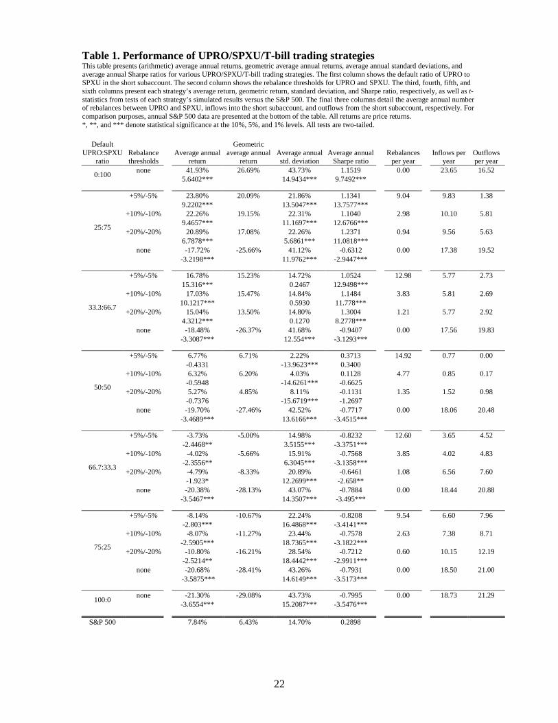
The main results of our simulations, including average annual returns, standard

deviations, and Sharpe ratios are presented in Table 1. The first column shows the default ratio of

UPRO to SPXU in the short subaccount. For example, 25:75 corresponds to trading strategies in

which the UPRO balance is three times lower than the SPXU balance at the start of the

simulation and after each rebalancing. The second column shows the rebalance thresholds. In the

case of the 25:75 strategy, +5%/-5% rebalancing means that UPRO and SPXU holdings are

rebalanced to the default ratio whenever the ratio breaches 20:80 or 30:70. Likewise, in the case

of the 33.3:66.7 strategy, +20%/-20% rebalancing means that UPRO and SPXU holdings are

rebalanced whenever the ratio breaches 13.3:86.7 or 53.3:46.7. The third, fourth, fifth, and sixth

columns present each strategy’s (arithmetic) average annual return, geometric average annual

return, average annual standard deviation, and average annual Sharpe ratio, respectively. For

annual returns, standard deviations, and Sharpe ratios, t-statistics from tests of each strategy’s

simulated results versus the S&P 500 appear below. The final three columns detail the average

annual number of rebalances between UPRO and SPXU, inflows into the short subaccount, and

5 In effect, the “maintenance margin” is assumed to be 90%, which is equal to FINRA’s currently mandated maintenance margin for shorting triple-leveraged and inverse triple-leveraged ETFs. For additional information, see FINRA’s Regulatory Notice 09-53, which is available at www.finra.org.

11

outflows from the short subaccount, respectively. For comparison purposes, annual S&P 500

data are presented at the bottom of the table.

Several important findings emerge from our simulations. First, as Table 1 shows, the best

performing strategy in terms of the Sharpe ratio is the 33.3:66.7 strategy with +20%/-20%

rebalancing. The investment yields an average annual Sharpe ratio of 1.3004 – more than four

times that of the S&P 500. Interestingly, the 33.3:66.7 portfolio with +5%/-5% rebalancing

produces a higher average return and a lower average standard deviation, yet a lower average

Sharpe ratio.6

Since the 33.3:66.7 strategy with +20%/-20% rebalancing performs better than any of the

others as measured by the Sharpe ratio, we focus primarily on this strategy (which we refer to as

Second, as the ratio of UPRO to SPXU increases, the annual return decreases, as

does the geometric annual return. Third, as the ratio of UPRO to SPXU increases, the standard

deviation decreases until we reach the 50:50 portfolio, after which it begins to increase. Fourth,

rebalancing is key for all portfolios other than the 0:100 portfolio. Without rebalancing, the

SPXU balance drops to near $0 over time, while the UPRO balance grows without limit. As a

result, given a long enough investment horizon, the strategy loses money. In the case of 0:100,

there is no investment in UPRO, and therefore the lack rebalancing is not a concern. Fifth,

inflows and outflows are most frequent for strategies that don’t entail rebalancing. Sixth, and not

surprising, tighter rebalancing thresholds lead to more frequent rebalancing. In practice, trading

triggered by inflows, outflows, and rebalancing has the potential to wipe out any profits because

of transaction costs imposed on the investor. We discuss transaction costs in more detail in

Section V.

6 Strategy A can have a lower average Sharpe ratio than strategy B despite a higher average return and a lower average standard deviation because the average Sharpe ratio is not the average difference between returns on the portfolio and the risk-free rate divided by the average portfolio standard deviation, but rather the average of the individual Sharpe ratios.

12

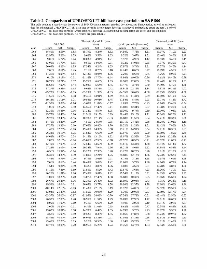
the base case) throughout the remainder of our paper. In Table 2 we present evidence that the

base case portfolio doesn’t merely outperform the S&P 500 over very long investment horizons,

but also consistently outperforms the market during 1-year holding periods. The table contains a

year-by-year breakdown of S&P 500 annual returns, standard deviations, and Sharpe ratios, as

well as annual returns, standard deviations, and Sharpe ratios for the base case portfolio. It shows

that the base case portfolio has outperformed the market in 43 of the 48 years between 1963 and

2010.

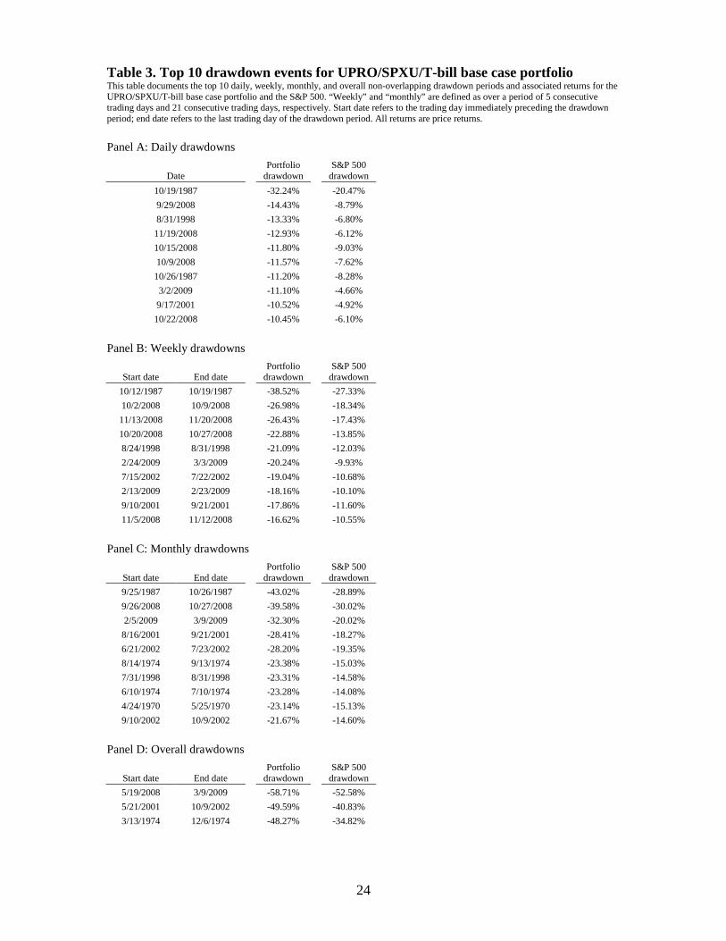
To assess potential losses from the base case strategy, we examine the top ten drawdown

events over 1-day, 1-week, 1-month, and unbounded non-overlapping periods. The results are

tabulated in Table 3. Panel A shows that the worst day for the portfolio during the 1963-2010

period would have been October 19, 1987. This coincides with the worst day for the S&P 500

during that period, which came to be known as Black Monday. That day the U.S. stock market

lost 20.47% of its value, while the base case portfolio would have lost 32.24%. The second worst

day for the portfolio would have been September 29, 2008, when it would have lost a relatively

modest 14.43% of its value as the market dropped by 8.79%. Panel B shows the top weekly

drawdowns, where a week is defined as 5 consecutive trading days. The worst week in recent

history was the 5-day stretch that ended on Black Monday, during which the portfolio lost

38.52%, while the market sank 27.33%. Panel C tabulates analogous figures for monthly

drawdowns. Once again, the worst period included Black Monday, with the portfolio losing

43.02% of its value as the market shed 28.89%. Finally, Panel D presents the top maximum

drawdown events during the period we study. We find that between 5/19/2008 and 3/9/2009 the

base case portfolio would have lost 58.71% of its value, as the market lost 52.58%. There are

other periods of large losses as well. It is important to note, however, that investors can limit

13

their losses by allocating part of their capital to the shorting strategy and part to other assets. In

particular, by investing in the shorting strategy and the Treasury bill (in addition to the T-bill

position already required by the shorting strategy) in carefully chosen proportions, an investor

can realize the same Sharpe ratios as in Tables 1 and 2, while keeping drawdowns (and

volatility) to the desired level.

V. Discussion

Dividends, tracking errors, transaction costs, fund fees and expenses, and taxes have

important implications for the performance of the trading strategies we consider. We now discuss

each of these in turn.

A. Dividends

Although we have been focusing on price returns, our results hold for total returns as

well. In particular, any shorting strategy that yields better risk-adjusted performance than the

S&P 500 in terms of price returns also produces better risk-adjusted performance than the market

in terms of total returns. More formally, assuming no tracking errors,

( ) ( ) implies p f m f p p f m m f

p m p m

r r r r r D r r D rσ σ σ σ− − + − + −

> > , (5)

where pr is the annual return on the portfolio, fr is the annual risk-free rate, pσ is the annualized

standard deviation of the portfolio, mr is the annual return on the market, mσ is the annualized

standard deviation of the market, and pD and mD are the dividend yields on the portfolio and the

market, respectively. Statement (5) follows because all dividends distributed by the component

14

stocks are paid in multiple to the bull LETF by its counterparty, and have to be paid in multiple

by the bear LETF to its counterparty, and the fact that,

( ) ( ) ( ) ( ) ( )p p f p f p m f p m f m m fm

p p p m p m m m

r D r r r D r r D r r r D rDλσ σ σ σ σ σ λσ σ

+ − − − − + −= + > + = + = , where λ is the total

exposure of the portfolio to the market, and the inequality is by assumption.

If a trading strategy is subject to tracking errors, as in our case, then (5) may not follow

because pσ may not equal mλσ . However, since UPRO’s and SPXU’s tracking errors are very

small compared to the difference in the base case portfolio’s and the market’s Sharpe ratios, our

findings are valid with respect to total returns.

B. Tracking errors

Tracking errors arise from a number of sources. First, since triple-leveraged ETFs and

inverse triple-leveraged ETFs pay 2× the risk-free interest rate and receive 4× the risk-free

interest rate, respectively,7

2 4UPRO SPXUw w× − ×

neither category of funds achieves its stated objective, even in theory,

unless the interest rate is 0%. When shorting a triple-leveraged ETF, the investor in effect pays

3× the underlying index return and receives 2× the interest rate, while when shorting an inverse

triple-leveraged ETF, the investor in effect receives 3× the underlying index return and pays 4×

the interest rate. Consequently, interest transfers “help” short UPRO positions and “hurt” short

SPXU positions. The effective interest rate exposure for an LETF shorting strategy is equal to

, where UPROw and SPXUw are the weights of UPRO and SPXU in the portfolio,

respectively. For a 33.3:66.7 strategy, the effective interest rate exposure is -2×. Despite the drag

on shorting strategy returns (for some portfolios) produced by interest transfers, all of our finding

7 See http://www.proshares.com/media/documents/components_of_leveraged_and_inverse_funds.pdf for an overview of how LETFs achieve their desired exposure to the underlying index.

15

ought to hold unless interest rates are high. As of 12/31/2012, the yield on the 30-year Treasury

bond was 2.95%, suggesting interest rates are expected to remain low for many years to come.

Also, note that we have been implicitly assuming that shorting (including shorting of LETFs)

does not generate cash that can be invested at the risk-free rate. If a brokerage pays interest on

short balances, it would mitigate the negative interest rate exposure created by a short SPXU

position.

Second, underleveraging (as well as overleveraging, which is not common) impacts

tracking errors, since the resulting fund returns are different from target returns. However,

underexposure decreases interest transfers discussed above, so it may bring actual returns closer

in line with target returns.

Third, residuals…, while the negative autocorrelation of residuals…

Fourth, fund fees and expenses may exacerbate tracking errors because they may create a

drag on LETF returns. Fees and expenses are discussed in more detail below.

C. Transaction costs

We can approximate transaction costs by using the data on trading frequencies, rebalance

thresholds, inflow/outflow thresholds, and bid-ask spreads. In particular, not counting

commissions and assuming rebalancing and inflows/outflows don’t occur on the same days,

average annual trading costs as a percentage of portfolio value can be expressed as,

2 2

2 2 2

UPRO SPXU

UPRO SPXU Tbill

s sR R

s s sUPRO IO SPXU IO IO

TC freq RT freq RT

w freq IOT w freq IOT freq IOT

= +

+ + +, (6)

16

where UPROs , SPXUs , and Tbills , are percentage bid-ask spreads for UPRO, SPXU, and Treasury

bills, respectively, Rfreq and IOfreq are the average annual number of rebalance and

inflow/outflow transactions, respectively, RT and IOT are the rebalance thresholds and

inflow/outflow thresholds, respectively, and UPROw and SPXUw are the weights of UPRO and

SPXU in the portfolio, respectively. According to IndexUniverse.com, the typical bid-ask

spreads for UPRO and SPXU are 0.04% and 0.03%, respectively. Assuming the typical spread

for T-bills is 0.08% (Chakravarty and Sarkar (2003)), average annual trading costs as a

percentage of portfolio value (for the base case) is approximately,

0.04% 0.03%.333,.667,.20 2 2

0.04% 0.03% 0.08%2 2 2

1.21) 1.21)

+

( )( (20%) ( )( (20%)

33.3%( )(5.77 (10%) 66.7%( )(5.72.92) + 2.92) + 2.92)0

7 (10%) ( )(5.77 .058%

(10%)

TC = +

+ + +

=

.

This is very low, and should not have a significant impact on the performance of the portfolio.

D. Fund fees and expenses

Unless the present value of expected future LETF fees and expenses is already reflected

in market prices, these operating costs create a drag on LETF returns. Consequently, fees and

expenses boost the performance of shorting strategies. For the funds we examine in this paper,

market values are very close to NAVs, so these costs do not appear to be impounded in prices.

All else equal, the higher the fees and expenses, the better the shorting strategy ought to perform.

As of December 2012, UPRO’s and SPXU’s annual expense ratios are 0.95% and 0.93%,

respectively, which ranks the two LETFs at the low end in terms of operating costs among all

triple-leveraged and inverse triple-leveraged ETFs.8

8 The average annual expense ratio for the universe of triple-leveraged and inverse triple-leveraged ETFs is 1.07%. The range is 0.93%–1.20%.

17

E. Taxes

Since short balances are marked to market, most tax obligations arising from favorable

performance of our investment strategies can be postponed indefinitely. Assuming positive

exposure to the market in the short subaccount (that is, a ratio of UPRO to SPXU of less than 1),

inflows imply unrealized gains in the short subaccount and unrealized gains in the long

subaccount, while outflows imply realized losses in the short subaccount and unrealized losses in

the long subaccount. Neither situation requires immediate payment of taxes. Rebalancing usually

leads to either unrealized gains for SPXU and realized losses for UPRO (when the market has

been going up), or realized losses for SPXU and unrealized gains for UPRO (when the market

has been going down), in which cases any tax obligations can also be postponed. Occasionally,

rebalancing leads to unrealized gains for one of the LETFs and realized gains for the other (when

the market has been going “sideways”), in which case taxes cannot be postponed. In sum, the tax

implications of our shorting strategies are predominantly favorable.

VI. Conclusion

Leveraged and inverse leveraged exchange traded funds have become very popular

financial products among investors since their introduction in 2006. These instruments allow

investors to amplify directional bets on an underlying index. However, over extended periods,

LETFs usually produce returns below that of the index times the leverage multiple. In fact, both

bull and bear funds linked to an index often underperform the index over the same period. With

this empirical observation in mind, we examine whether taking simultaneous short positions in

triple-leveraged and inverse triple-leveraged ETFs can yield a higher Sharpe ratio than that of the

S&P 500.

18

Since LETFs are a relatively new financial innovation, we simulate daily returns on a

triple leveraged and an inverse triple leveraged fund over a period of 48 years. Our simulation

design allows us to preserve a number of statistical properties of returns on a pair of actual funds,

and calibrate them to the market returns during the period we investigate. To our knowledge, this

is the first paper that attempts to explicitly estimate how these funds would have performed over

the years. We find that many of the strategies we examine produce superior portfolio

performance as measured by the Sharpe ratio. The optimal strategy appears to be one that shorts

the bear LETF and the bull LETF in a 2:1 proportion, yielding an average Sharpe ratio that is

more than four times higher than that of the S&P 500. This strategy also appears to be highly

consistent in outperforming the market on a risk-adjusted basis.

19

Appendix

We simulate tracking errors, ,UPRO tε and ,SPXU tε , via the following procedure: First, we generate

two independent sequences of standard normal random variables, 1,1 1,2 1,, ,..., Nz z z and

2,1 2,2 2,, ,..., Nz z z . Next, we define 3, 1 2,2

, (1 (0.7440 0.7440) )t t tz z z= − + −− . The parameter –0.7440 is

from (3), and introduces cross-correlation between 1,tz and 3,tz . Next, we let 1, 1, 1

2

(z z )

1,UPRO

UPR

t t

OUPRO t

γ

γθ +−

+=

and 3, 3, 1

2

(z z )

1,SPXt t

SPXU

USPXU t

γ

γθ +−

+= , where

21 4( 0.4622)2( 0.46

12

(2)UPROγ − −+ −

−= and 21 4( 0.4890)

2( 0.481

9(

0)SPXUγ − −+ −−= . The parameters

-0.4622 and -0.4890 are again from (3), and introduce first-order autocorrelation (while keeping

higher-order autocorrelations at zero) in ,UPRO tθ and ,SPXU tθ . Finally, we center and scale the

variables by letting , ,,

,0.00227

( )UPRO t UPRO t

UPRO tUPRO tSD

θ θε

θ−

= and , ,,

,0.00207

( )SPXU t SPXU t

SPXU tSPXU tSD

θ θε

θ−

= , where

( )SD denotes sample standard deviation, bar denotes sample mean, and the parameters 0.00227

and 0.00207 are from (3).

20

References Avellaneda, Marco and Stanley Zhang, 2009, Path-dependence of leveraged ETF returns, working paper, New York University. Bai, Qing, Shaun A. Bond and Brian Hatch, 2012, The Impact of Leveraged and Inverse ETFs on Underlying Stock Returns, working paper, University of Cincinnati. Chakravarty, Sugato and Asani Sarkar, 2003, Trading costs in three U.S. bond markets, Journal of Fixed Income 13, 39-48. Charupat, Narat and Peter Miu, 2011, The pricing and performance of leveraged exchange-traded funds, Journal of Banking and Finance 35, 966-977. Cheng, Minder and Ananth Madhavan, 2009, The dynamics of leveraged and inverse exchange-traded funds, Journal of Investment Management 7, 43-62. Dulaney, Tim, Tim Husson, and Craig McCann, 2012, Leveraged, inverse, and futures-based ETFs, PIABA Bar Journal 19, No. 1. Haryanto, Edgar, Arthur Rodier, Pauline Shum, and Walid Hejazi, 2012, Intraday share price volatility and leveraged ETF rebalancing, working paper, York University. Jarrow, Robert A., 2010, Understanding the risk of leveraged ETFs, Finance Research Letters 7, 135–139. Kephart, Jason, Market volatility? Don't blame ETFs, says ICI, Investment News, 23 February, 2012, accessed on 1/3/2012 at http://www.investmentnews.com/article/20120223/FREE/120229965. Lauricella, Tom, ETF math lesson: Leverage can produce unexpected returns, Wall Street Journal, 4 January, 2009, accessed on 12/22/2012 at http://online.wsj.com/article/SB123111094917552317.html. Leung, Tim and Marco Santoli, 2012, Leveraged ETFs: Admissible leverage and risk horizon, working paper, Columbia University. Lu, Lei, Jun Wang and Ge Zhang, 2012, Long term performance of leveraged ETFs, Financial Services Review 21, 63–80. Shum, Pauline M. and Jisok Kang, 2012, The long and short of leveraged ETFs: The financial crisis and performance attribution, working paper, York University. Sorkin, Andrew Ross, Volatility, Thy Name is E.T.F., New York Times, 10 October, 2011, accessed on 1/3/2012 at http://dealbook.nytimes.com/2011/10/10/volatility-thy-name-is-e-t-f.

21

Tang, Hongfei and Xiaoqing Eleanor Xu, 2012, Solving the return deviation conundrum of leveraged exchange-traded funds, Journal of Financial and Quantitative Analysis, forthcoming. Wang, Zhenyu, 2009, Market efficiency of leveraged ETFs, working paper, Federal Reserve Bank of New York.

22

Table 1. Performance of UPRO/SPXU/T-bill trading strategies This table presents (arithmetic) average annual returns, geometric average annual returns, average annual standard deviations, and average annual Sharpe ratios for various UPRO/SPXU/T-bill trading strategies. The first column shows the default ratio of UPRO to SPXU in the short subaccount. The second column shows the rebalance thresholds for UPRO and SPXU. The third, fourth, fifth, and sixth columns present each strategy’s average return, geometric return, standard deviation, and Sharpe ratio, respectively, as well as t-statistics from tests of each strategy’s simulated results versus the S&P 500. The final three columns detail the average annual number of rebalances between UPRO and SPXU, inflows into the short subaccount, and outflows from the short subaccount, respectively. For comparison purposes, annual S&P 500 data are presented at the bottom of the table. All returns are price returns. *, **, and *** denote statistical significance at the 10%, 5%, and 1% levels. All tests are two-tailed.

Default UPRO:SPXU

ratio Rebalance thresholds

Average annual return

Geometric average annual

return Average annual std. deviation

Average annual Sharpe ratio

Rebalances per year

Inflows per year

Outflows per year

0:100 none

41.93% 26.69% 43.73% 1.1519

0.00

23.65 16.52

5.6402***

14.9434*** 9.7492***

25:75

+5%/-5%

23.80% 20.09% 21.86% 1.1341

9.04

9.83 1.38

9.2202***

13.5047*** 13.7577***

+10%/-10%

22.26% 19.15% 22.31% 1.1040

2.98

10.10 5.81

9.4657***

11.1697*** 12.6766***

+20%/-20%

20.89% 17.08% 22.26% 1.2371

0.94

9.56 5.63

6.7878***

5.6861*** 11.0818***

none

-17.72% -25.66% 41.12% -0.6312

0.00

17.38 19.52

-3.2198***

11.9762*** -2.9447***

33.3:66.7

+5%/-5%

16.78% 15.23% 14.72% 1.0524

12.98

5.77 2.73

15.316***

0.2467 12.9498***

+10%/-10%

17.03% 15.47% 14.84% 1.1484

3.83

5.81 2.69

10.1217***

0.5930 11.778***

+20%/-20%

15.04% 13.50% 14.80% 1.3004

1.21

5.77 2.92

4.3212***

0.1270 8.2778***

none

-18.48% -26.37% 41.68% -0.9407

0.00

17.56 19.83

-3.3087***

12.554*** -3.1293***

50:50

+5%/-5%

6.77% 6.71% 2.22% 0.3713

14.92

0.77 0.00

-0.4331

-13.9623*** 0.3400

+10%/-10%

6.32% 6.20% 4.03% 0.1128

4.77

0.85 0.17

-0.5948

-14.6261*** -0.6625

+20%/-20%

5.27% 4.85% 8.11% -0.1131

1.35

1.52 0.98

-0.7376

-15.6719*** -1.2697

none

-19.70% -27.46% 42.52% -0.7717

0.00

18.06 20.48

-3.4689***

13.6166*** -3.4515***

66.7:33.3

+5%/-5%

-3.73% -5.00% 14.98% -0.8232

12.60

3.65 4.52

-2.4468**

3.5155*** -3.3751***

+10%/-10%

-4.02% -5.66% 15.91% -0.7568

3.85

4.02 4.83

-2.3556**

6.3045*** -3.1358***

+20%/-20%

-4.79% -8.33% 20.89% -0.6461

1.08

6.56 7.60

-1.923*

12.2699*** -2.658**

none

-20.38% -28.13% 43.07% -0.7884

0.00

18.44 20.88

-3.5467***

14.3507*** -3.495***

75:25

+5%/-5%

-8.14% -10.67% 22.24% -0.8208

9.54

6.60 7.96

-2.803***

16.4868*** -3.4141***

+10%/-10%

-8.07% -11.27% 23.44% -0.7578

2.63

7.38 8.71

-2.5905***

18.7365*** -3.1822***

+20%/-20%

-10.80% -16.21% 28.54% -0.7212

0.60

10.15 12.19

-2.5214**

18.4442*** -2.9911***

none

-20.68% -28.41% 43.26% -0.7931

0.00

18.50 21.00

-3.5875***

14.6149*** -3.5173***

100:0 none

-21.30% -29.08% 43.73% -0.7995

0.00

18.73 21.29

-3.6554***

15.2087*** -3.5476***

S&P 500

7.84% 6.43% 14.70% 0.2898

23

Table 2. Comparison of UPRO/SPXU/T-bill base case portfolio to S&P 500 This table contains a year-by-year breakdown of S&P 500 annual returns, standard deviations, and Sharpe ratios, as well as analogous data for a theoretical UPRO/SPXU/T-bill base case portfolio (where target leverage is achieved and tracking errors are zero), a hybrid UPRO/SPXU/T-bill base case portfolio (where empirical leverage is assumed but tracking errors are zero), and the simulated UPRO/SPXU/T-bill base case portfolio. All returns are price returns.

S&P 500

Theoretical portfolio (base case)

Hybrid portfolio (base case)

Simulated portfolio (base case)

Year Return SD Sharpe

Return SD Sharpe

Return SD Sharpe

Return SD Sharpe 1963 18.89% 8.55% 1.83

15.79% 8.24% 1.52

14.98% 7.78% 1.51

19.07% 7.10% 2.23

1964 12.97% 5.26% 1.75

9.62% 3.58% 1.63

9.32% 3.67% 1.51

12.40% 3.49% 2.48 1965 9.06% 6.77% 0.74

10.03% 4.91% 1.21

9.57% 4.90% 1.12

11.53% 3.40% 2.19

1966 -13.09% 11.78% -1.55

0.81% 14.05% -0.31

0.32% 14.03% -0.35

-3.37% 18.35% -0.47 1967 20.09% 8.28% 1.85

17.54% 8.24% 1.55

17.97% 5.74% 2.31

27.37% 5.46% 4.14

1968 7.66% 8.61% 0.25

7.11% 8.75% 0.18

12.24% 8.65% 0.77

16.09% 4.57% 2.31 1969 -11.36% 9.98% -1.84

-12.12% 18.04% -1.06

2.20% 8.68% -0.55

5.26% 8.05% -0.21

1970 0.10% 15.19% -0.51

-21.16% 17.70% -1.64

-8.94% 19.60% -0.86

-8.62% 18.40% -0.89 1971 10.79% 10.21% 0.57

15.75% 6.65% 1.63

10.90% 12.05% 0.50

17.44% 8.17% 1.53

1972 15.63% 7.92% 1.44

12.98% 5.64% 1.55

13.47% 3.71% 2.50

14.99% 5.79% 1.86 1973 -17.37% 15.83% -1.55

-0.62% 18.71% -0.42

-18.91% 22.79% -1.14

6.81% 16.31% -0.02

1974 -29.72% 21.82% -1.75

-33.29% 31.33% -1.33

-24.55% 30.69% -1.08

-38.75% 29.99% -1.58 1975 31.55% 15.60% 1.58

30.31% 13.91% 1.69

39.51% 11.31% 2.89

46.10% 12.19% 3.22

1976 19.15% 11.11% 1.21

20.56% 10.08% 1.48

17.54% 5.84% 2.03

19.74% 8.16% 1.72 1977 -11.50% 9.08% -1.86

-3.65% 11.84% -0.77

2.09% 7.73% -0.43

-1.84% 13.46% -0.54

1978 1.06% 12.57% -0.50

14.56% 17.49% 0.41

15.60% 12.34% 0.67

19.38% 17.20% 0.70 1979 12.31% 10.85% 0.16

27.32% 8.57% 1.95

19.30% 9.74% 0.89

29.10% 7.08% 2.61

1980 25.77% 16.46% 0.80

31.51% 19.15% 0.99

38.44% 15.10% 1.71

40.34% 16.20% 1.71 1981 -9.73% 13.46% -1.95

10.78% 17.14% -0.33

16.88% 11.57% 0.04

22.41% 10.32% 0.58

1982 14.76% 18.26% 0.09

4.51% 24.54% -0.35

29.71% 24.42% 0.68

38.28% 21.02% 1.19 1983 17.27% 13.33% 0.60

27.66% 10.80% 1.70

26.32% 11.24% 1.51

21.42% 7.86% 1.54

1984 1.40% 12.75% -0.76

19.40% 14.39% 0.58

19.21% 14.91% 0.54

22.71% 18.36% 0.63 1985 26.33% 10.16% 1.75

21.83% 6.65% 2.00

23.07% 7.26% 2.00

28.19% 7.89% 2.49

1986 14.62% 14.70% 0.54

24.15% 13.16% 1.32

18.07% 12.55% 0.90

24.99% 12.28% 1.48 1987 2.03% 32.15% -0.14

-25.65% 47.56% -0.68

-27.92% 48.58% -0.71

-10.52% 41.65% -0.41

1988 12.40% 17.09% 0.32

32.54% 13.50% 1.90

31.81% 13.31% 1.88

29.94% 13.44% 1.72 1989 27.25% 13.05% 1.40

29.34% 7.94% 2.56

28.21% 8.63% 2.22

34.98% 6.58% 3.94

1990 -6.56% 15.97% -0.94

13.22% 17.33% 0.28

13.22% 18.23% 0.26

7.91% 22.17% -0.02 1991 26.31% 14.30% 1.39

27.80% 12.24% 1.75

28.88% 12.12% 1.86

37.23% 12.62% 2.44

1992 4.46% 9.71% 0.06

9.79% 2.66% 2.21

8.78% 3.13% 1.55

9.97% 4.69% 1.29 1993 7.06% 8.63% 0.44

10.49% 5.09% 1.42

11.00% 5.72% 1.36

14.96% 6.72% 1.74

1994 -1.54% 9.84% -0.59

8.32% 3.83% 1.06

8.08% 4.69% 0.81

10.78% 3.83% 1.70 1995 34.11% 7.81% 3.59

21.55% 4.52% 3.42

21.57% 3.66% 4.23

23.26% 4.39% 3.91

1996 20.26% 11.81% 1.26

17.43% 9.81% 1.22

15.54% 11.18% 0.91

24.33% 6.71% 2.82 1997 31.01% 18.23% 1.40

33.07% 17.48% 1.58

36.88% 10.30% 3.05

35.86% 15.68% 1.94

1998 26.67% 20.25% 1.06

32.39% 26.49% 1.02

26.59% 29.03% 0.73

3.35% 20.34% -0.10 1999 19.53% 18.04% 0.81

26.65% 13.77% 1.58

26.98% 12.37% 1.78

31.68% 13.66% 1.96

2000 -10.14% 22.18% -0.73

11.43% 27.19% 0.19

11.12% 24.06% 0.21

22.52% 19.51% 0.84 2001 -13.04% 21.37% -0.82

-31.55% 30.03% -1.20

-6.30% 29.06% -0.37

-12.99% 32.17% -0.54

2002 -23.37% 26.00% -0.97

-21.95% 34.03% -0.70

-17.54% 37.73% -0.51

-15.44% 32.50% -0.53 2003 26.38% 17.03% 1.48

28.95% 21.54% 1.29

26.69% 17.96% 1.42

32.61% 20.65% 1.52

2004 8.99% 11.07% 0.69

9.31% 6.67% 1.20

9.50% 3.90% 2.10

13.31% 3.96% 3.03 2005 3.00% 10.27% -0.01

9.10% 11.01% 0.55

9.62% 8.54% 0.77

12.34% 6.83% 1.35

2006 13.62% 10.01% 0.88

14.78% 6.42% 1.55

14.99% 3.73% 2.73

16.07% 9.35% 1.20 2007 3.53% 15.93% -0.10

20.52% 8.35% 1.85

11.86% 17.88% 0.38

21.74% 10.97% 1.52

2008 -38.49% 40.97% -0.99

-36.07% 53.33% -0.71

-37.08% 57.33% -0.68

-31.91% 64.05% -0.53 2009 23.45% 27.26% 0.85

9.27% 30.58% 0.30

2.24% 29.22% 0.07

0.71% 31.45% 0.02

2010 12.78% 18.05% 0.70

18.96% 15.23% 1.24

19.75% 14.73% 1.33

17.94% 25.51% 0.70

24

Table 3. Top 10 drawdown events for UPRO/SPXU/T-bill base case portfolio This table documents the top 10 daily, weekly, monthly, and overall non-overlapping drawdown periods and associated returns for the UPRO/SPXU/T-bill base case portfolio and the S&P 500. “Weekly” and “monthly” are defined as over a period of 5 consecutive trading days and 21 consecutive trading days, respectively. Start date refers to the trading day immediately preceding the drawdown period; end date refers to the last trading day of the drawdown period. All returns are price returns. Panel A: Daily drawdowns

Date

Portfolio drawdown

S&P 500 drawdown

10/19/1987

-32.24%

-20.47% 9/29/2008

-14.43%

-8.79%

8/31/1998

-13.33%

-6.80% 11/19/2008

-12.93%

-6.12%

10/15/2008

-11.80%

-9.03% 10/9/2008

-11.57%

-7.62%

10/26/1987

-11.20%

-8.28% 3/2/2009

-11.10%

-4.66%

9/17/2001

-10.52%

-4.92% 10/22/2008

-10.45%

-6.10%

Panel B: Weekly drawdowns

Start date End date

Portfolio drawdown

S&P 500 drawdown

10/12/1987 10/19/1987

-38.52%

-27.33% 10/2/2008 10/9/2008

-26.98%

-18.34%

11/13/2008 11/20/2008

-26.43%

-17.43% 10/20/2008 10/27/2008

-22.88%

-13.85%

8/24/1998 8/31/1998

-21.09%

-12.03% 2/24/2009 3/3/2009

-20.24%

-9.93%

7/15/2002 7/22/2002

-19.04%

-10.68% 2/13/2009 2/23/2009

-18.16%

-10.10%

9/10/2001 9/21/2001

-17.86%

-11.60% 11/5/2008 11/12/2008

-16.62%

-10.55%

Panel C: Monthly drawdowns

Start date End date

Portfolio drawdown

S&P 500 drawdown

9/25/1987 10/26/1987

-43.02%

-28.89% 9/26/2008 10/27/2008

-39.58%

-30.02%

2/5/2009 3/9/2009

-32.30%

-20.02% 8/16/2001 9/21/2001

-28.41%

-18.27%

6/21/2002 7/23/2002

-28.20%

-19.35% 8/14/1974 9/13/1974

-23.38%

-15.03%

7/31/1998 8/31/1998

-23.31%

-14.58% 6/10/1974 7/10/1974

-23.28%

-14.08%

4/24/1970 5/25/1970

-23.14%

-15.13% 9/10/2002 10/9/2002

-21.67%

-14.60%

Panel D: Overall drawdowns

Start date End date

Portfolio drawdown

S&P 500 drawdown

5/19/2008 3/9/2009

-58.71%

-52.58% 5/21/2001 10/9/2002

-49.59%

-40.83%

3/13/1974 12/6/1974

-48.27%

-34.82%

25

10/5/1987 10/26/1987

-43.97%

-30.61% 11/10/1969 5/26/1970

-33.39%

-29.53%

7/17/1998 8/31/1998

-27.47%

-19.34% 2/1/2001 4/4/2001

-24.87%

-19.67%

7/16/1990 10/11/1990

-24.02%

-19.92% 4/21/1966 10/7/1966

-23.40%

-20.80%

4/23/2010 7/2/2010

-18.75%

-15.99%

26

Figure 1. UPRO, SPXU, and S&P 500 returns during 4/1/10 - 4/7/10 (top) and 4/1/10 - 10/1/11 (bottom)

Source: http://money.msn.com

27

Figure 2. UPRO, SPXU, and S&P 500 returns during 11/21/2011 - 4/2/2012

Source: http://money.msn.com