Embed Size (px)
Citation preview

Investment Incentives in Tradable Emissions Markets with Price Floors∗
Timothy N. Casona John K. Stranlundb Frans P. de Vriesc
aDepartment of Economics, Krannert School of Management, Purdue University, USAbDepartment of Resource Economics, University of Massachusetts-Amherst, USAcDivision of Economics, University of Stirling Management School, Scotland UK
July 11, 2021
Abstract
Concerns about cost containment and price volatility have led regulators to include pricecontrols in many cap-and-trade markets. We study how these controls affect firms’ incen-tives to invest in new abatement technologies in a model with abatement cost uncertainty.Price floors increase investment incentives because they raise the expected benefits fromlowering abatement costs. We also report a market experiment that features abatement costuncertainty and the opportunity for cost-reducing investment, with and without a price floor.Trade occurs through a continuous double auction market. Consistent with the theoreticalmodel, investment is significantly greater with the price floor in place. Emissions permitprices also respond as predicted to abatement investments and emissions shocks.
Keywords: Emissions trading; Technological innovation; Price controls; Market design; Lab-oratory experiments
JEL Classification: C91; D47; O33; Q55; Q58
∗We thank Lata Gangadharan, Lana Friesen, Neslihan Uler and audiences at the EAERE and ESA conferencesfor valuable comments on an earlier draft, and Jim Murphy for some early suggestions on the experimental design.We also thank Peter Wagner and Stanton Hudja for programming assistance. This research is approved by thePurdue University IRB (Protocol number 1902021679).
1
1 Introduction
A fundamental issue in market-based environmental policy is the extent to which tradable emis-
sions markets can steer investment towards energy-saving and advanced abatement technology
in the long run. In the context of climate change, for instance, investment in developing and
adopting low-carbon technologies is crucial to reducing the cost of climate mitigation. Some car-
bon permit markets, however, have experienced considerable price volatility, particularly some
extremely low prices. For example, allowance prices in the European Union Emissions Trading
System (EU ETS) were below e10 per ton from November 2011 to February 2018. Current
prices exceed e30 per ton. Allowance auction clearing prices in the Regional Greenhouse Gas
Initiative (RGGI) were at the very low reserve price (set at $1.86 per ton in 2008, increasing
slowly to $2.26 in June 2019) for auctions conducted between June 2010 and December 2012,
and has only rarely exceeded $6.00 per ton (US Congressional Research Service, 2019). Simi-
larly, in California’s cap-and-trade market for greenhouse gases, auction prices and secondary
market prices have been at or close to the auction reserve price throughout the program’s history
(California Air Resources Board, 2021). Lower-than-expected prices can undermine investors’
confidence in future market conditions, adversely affecting the expected rewards from invest-
ment strategies (Burtraw et al., 2010), and resulting in reduced investment in environmental
innovation (Taylor, 2012). Introducing price floors can guard against the threat of (too) low
allowance prices, and the potential for under-investment in abatement technology (Philibert,
2009; Wood and Jotzo, 2011).1
However, the theoretical and empirical literature concerning the effects of price floors on
investment in abatement technologies is limited, and to some degree non-integrated. Our paper
tries to fill this gap. First, we develop a formal, tractable model of an emissions trading market
comprising heterogeneous firms that allows us to make theoretical predictions about the firms’
investment decisions, with and without a price floor. Second, we test this model’s predictions
in a market experiment, providing empirical evidence on investment behavior in such market
conditions.2 Our main research question is: how does the introduction of a price floor in
emissions trading markets affect firms’ incentives to invest in cost-saving abatement technologies?
Our theoretical model suggests that in a market with a mix of firms that invest and do
not invest in a cost-reducing technology, only firms with high abatement costs will invest in the
technology. The introduction of a price floor expands the set of investors to include medium-cost
firms who would not invest in the absence of the price floor. The results of our experiments are
1Incorporating price controls in emissions markets was first suggested by Roberts and Spence (1976). Althoughthey considered implementing both price ceilings and price floors, the first recommendations for controlling abate-ment cost uncertainty in carbon markets focused on price ceilings (Pizer, 2002; Jacoby and Ellerman, 2004).However, a price ceiling cannot address the problem of low-side abatement cost risk, and it has become evidentthat emissions markets are more often plagued by (too) low prices rather than price spikes (Burtraw et al., 2010).
2We restrict our attention to the implementation of price floors in existing tradable emissions markets andtheir effects on investment in abatement technology. Our experimental evidence is unique for such settings, butcomplements empirical research on feed-in tariffs and investment in renewable energy technologies (e.g., Johnstoneet al., 2010). Feed-in tariffs tend to be long-term contracts for renewable energy at minimum prices above marketprices to encourage adoption of renewable energy (e.g., Tanaka et al., 2017). In this respect, feed-in tariffs actlike the price floors in our model.
2

consistent with these hypotheses. The main policy lesson is clear: a price floor in an emissions
market can motivate increased investment in technologies that reduce firms’ abatement costs.
Although outside the scope of our analysis, a logical conjecture is that this additional demand
for cost-reducing technologies can spur additional innovation in abatement technologies.
Our work contributes to the theoretical and experimental literature on price controls in
emissions markets. In the last decade, the theoretical literature expanded to include analyses of
alternative price stabilization schemes (Fell et al., 2012; Grull and Taschini, 2011); the relation-
ship between price controls and banking (Fell and Morgenstern, 2010); and the optimal design
of emissions markets with price controls accounting for enforcement (Stranlund and Moffitt,
2014) and co-pollutants (Stranlund and Son, 2019). A recent study by Borenstein et al. (2019)
highlights the continuing importance of analyzing the design and effects of implementing price
controls, because their work reveals that relatively large uncertainty in business-as-usual emis-
sions implies that permit prices are likely to be determined by price floors and ceilings rather
than permit supplies.
The experimental literature addressing price controls and other price stabilization policies
is more limited than the theoretical literature. Building on the seminal work of Isaac and
Plott (1981) and Smith and Williams (1981) who examined price controls in laboratory settings,
the more recent experimental literature related to the design of emissions markets has mainly
focused on comparing alternative schemes in terms of their ability to limit permit price risk. For
example, Stranlund et al. (2014) studied the effects of price controls and banking, separately and
together. Holt and Shobe (2016) examined alternative price and quantity controls motivated
by the market stability reserve of the EU ETS. Perkis et al. (2016) examined hard and soft
price ceilings, while Friesen et al (2019) examined soft price ceilings with an alternative design
for auctioned permits. Here we examine a hard price floor, which entails a lower absolute limit
on the permit price. This can be implemented in markets where allowances are distributed for
free and where the government commits to buy back any unused allowances at the floor price.3
Friesen et al. (2020) investigated the use of dual allowance reserves and trigger prices. Finally,
Salant et al. (2020) studied the impact of non-binding hard and soft floors on permit prices in
a dynamic setting with permit banking. In contrast to these studies of alternative mechanisms
to stabilize permit prices, we examine the effects of a hard price floor on investments in a
cost-saving abatement technology under uncertainty.
None of the aforementioned papers is concerned with the effects of price controls on invest-
ments in cost-reducing abatement technologies. To our knowledge, only Weber and Neuhoff
(2010) and Brauneis et al. (2013) addressed technology investments and price controls in emis-
sions markets. In particular, Weber and Neuhoff is a normative theoretical study of the optimal
design of an emissions market with price controls; however, they do not address how price con-
trols affect firms’ investments in reducing their abatement costs. Brauneis et al. employ a
simulation model in conjunction with a real options approach to determine the optimal carbon
3In contrast, in emissions markets where allowances are auctioned, a soft price floor can be implementedthrough a minimum reserve price for newly auctioned permits (see Murray et al., 2009).
3

price floor and its effect on the timing of investment in low-carbon technology in the electricity
sector. In contrast to these two papers, our contribution is a positive study that examines how
a price floor affects the adoption of a cost-saving abatement technology, both theoretically and
experimentally.
In this respect, our paper also adds to the literature on environmental policy induced tech-
nology adoption (for a survey, see Requate, 2005).4 Under certainty about firm’s abatement
costs, Requate and Unold (2003) argued that a fixed emissions tax provides a greater incentive
for firms to adopt a cost-saving technology than a competitive emissions market with a fixed
number of emissions permits. The reason is that a significant number of adopters will lower
the permit price in a market, which in turn reduces the adoption incentive and the number
of adopters. We show, both theoretically and experimentally, that adding a price floor to an
emissions market under uncertainty about firms’ abatement costs can increase the adoption in-
centives in the market and increase the number of adopters of a new technology. This occurs
because the price floor truncates the lower range of potential permit prices when abatement
costs are uncertain.
The paper is structured as follows. In Section 2 we develop the theory and derive the main
propositions. The experimental design, implementation and hypotheses are described in Section
3, followed by the analyses and discussion of results in Section 4. Conclusions are drawn in
Section 5.
2 Theoretical Framework
Our experiment is based on a theoretical model of n heterogeneous risk-neutral competitive
firms who participate in a market to control a uniformly mixed pollutant. Firm i in the market
emits qi units of a pollutant and its abatement cost function is
ai(qi, u) =
∫ qi0
qi(bi + u− cqi)dqi, (1)
where bi and c are positive constants. The random variable u affects the abatement costs of
all firms, and is distributed on support [u, u] with probability density function g(u) and zero
expectation.5 Finally, qi0 is the minimizer of ai(qi, u); that is, qi0(u) = (bi + u)/c, with bi > u for
each firm. This is commonly referred to as the firm’s unregulated level of emissions.
Firms can make an investment to reduce their total and marginal abatement costs while
4Generally, our work fits into a broader literature that studies how market design can affect market performanceby affecting investment decisions (Fabra et al., 2011).
5The firm’s marginal abatement cost function is linear with uncertainty in the intercepts, which is frequentlyassumed in the theoretical and experimental literature on emissions control instrument choice, including policiesinvolving price controls (e.g., Weitzman 1974; Weber and Neuhoff, 2010, Fell et al., 2012; Stranlund et al., 2014;Stranlund and Son, 2019). Due to the way in which this common shock u enters the abatement cost function, itcould also be thought of as a common shock to emissions, given an emissions price. This could arise, for example,through regional weather variation or macroeconomic shocks (such as, most dramatically, a global pandemic).
4
holding the slope of the marginal abatement cost function constant.6
bi = bi(1− βxi), (2)
where xi = {0, 1} is an irreversible dichotomous investment choice, bi is a positive constant that
varies across firms on the interval [bmin, bmax], and β ∈ (0, 1) is a constant that does not vary
across firms. Combining equations (1) and (2) allows us to rewrite the firm’s abatement cost
function as
ai(qi, xi, u) =(bi(1− βxi) + u)2
2c− (bi(1− βxi) + u)qi +
c(qi)2
2. (3)
Firms are distinguished from one another by the level of the parameter bi, which we will some-
times refer to as firm i’s “type.”
We analyze an emissions trading program with and without a price floor with the following
features. A total of L permits are distributed to the firms (free of charge), and firm i receives
li0 permits from this initial distribution. Each permit confers the legal right to emit one unit of
emissions and enforcement is assumed to be perfect, implying that firms’ final permit holdings
are equal to their emissions. Emissions permits trade at a competitive price p. When the market
includes a price floor the government commits to buying back unused permits at a fixed price
s. For the market to clear we must have s ≤ p. Throughout we assume that the price floor has
a strictly positive probability of binding.
The timing of events in our model is as follows. Given the elements of the market policy, in
the first stage all firms choose whether to make their irreversible investments in reducing their
abatement costs. In the second stage the value of u is revealed and, given u, firms choose their
emissions, trade in the permit market (including potential sales to the government), the market
clears, and the firms release their allowed levels of emissions.7
2.1 A Pure Market without Price Controls
In this subsection we specify the equilibrium for a market without a price floor, starting with
the second stage. Given the realization of u, a permit price (to be determined) and investments
from the first stage, a firm chooses its emissions to minimize its compliance cost, consisting of
its abatement cost and the value of its permit transactions:
ci(qi, xi, u) = ai(qi, xi, u) + p(qi − li0)
=(bi(1− βxi) + u)2
2c− (bi(1− βxi) + u)qi +
c(qi)2
2+ p(qi − li0). (4)
6Our research question is centered around the incentives to invest in the adoption of an existing cost-savingabatement technology. An alternative design could relate to investment in R&D and feature stochastic investmentsuccess (see Cason and de Vries, 2019). This would, however, imply a random shock at the firm level in additionto the common shock that affects the abatement costs of all firms as in our current setup (see also footnote 5).We leave investigation of this more complex design for future research.
7The model is static, which precludes a real options approach to analyzing investments under uncertainty. Zhao(2003) takes a real options approach to show how abatement cost uncertainty affects irreversible investments inabatement capital or technologies under emissions markets and emissions taxes. To our knowledge there is nopublished work that extends this approach to consider investments under emissions markets with price controls.
5
The familiar rule of equalizing marginal abatement cost and the permit price gives us the firm’s
choice of emissions,
qi(xi, p, u) =bi(1− βxi) + u− p
c. (5)
Using (5) to solve the market clearing condition,∑n
i=1 qi(xi, p, u) = L, the equilibrium permit
price is
p(x, u) =
∑ni=1 b
i(1− βxi)− cLn
+ u, (6)
where x = (x1, ..., xn) is the vector of individual investments in abatement cost reductions.
Clearly the permit price is lower when the random variable u is lower and when more firms
invest in reducing their abatement costs. (Throughout we ignore the fact that the permit price
also depends on the supply of permits.)
It is convenient to write (6) as
p(x, u) = p(x) + u, (7)
where p(x) is the expected permit price (i.e., when u = 0), given investments x. Substitute (5)
and (7) into (4) to obtain a firm’s equilibrium compliance cost in the second stage as a function
of the first-stage investment
ci(x, u) = (p(x) + u)
(bi(1− βxi) + u
c− p(x) + u
2c− li0
). (8)
Having characterized the second-stage equilibrium emissions, permit price and firms’ com-
pliance costs, we are now in a position to consider a firm’s choice of investment in reducing its
abatement cost in the first stage. We begin by calculating a firm’s expected benefit of invest-
ment, given the investment choices of the other firms. Given a realization of u, the change in
firm i’s compliance cost if it invests in the first stage is
∆ci(x, u) = ci(xi = 1, x−i, u)− ci(xi = 0, x−i, u), (9)
where x−i = x\(xi). It is possible that a single firm’s investment in reducing its abatement
cost in the first stage can influence the equilibrium permit price in the second stage, and this
in turn can have an indirect effect on its decision to invest. To investigate this possibility, write
p(xi, x−i, u) = p(x, u) and use (6) to calculate the change in the equilibrium permit price with
i’s investment,
∆ip = p(xi = 1, x−i, u)− p(xi = 0, x−i, u) = −biβ
n< 0. (10)
We can see that the effect of a firm’s investment on the equilibrium permit price will be negligible
in a market with a relatively large number of participants, as in most real emissions markets. To
model these cases we set ∆ip = 0. The propositions that we derive below and the corresponding
experimental hypotheses are based on this case. However, experimental emissions markets typi-
cally have a small number of participants, as do some emissions markets in practice.8 Therefore,
we will also address the small-number case when ∆ip < 0.
8For example, permit markets for effluent emissions to waterways sometimes have a small number of largeemitters, as discussed in Cason et al. (2003).
6
Define a firm’s expected reduction in its compliance cost from its investment in the first
stage as
ri(x) = −E(∆ci(x, u)
), (11)
where E denotes the expectation operator. In Appendix A we show that
∆ci(x, u) = ∆ip
(bi − p(xi = 0, x−i)
c− li0 −
∆ip
2c
)− (p(xi = 1, x−i) + u)biβ
c. (12)
Taking the expectation of (12) and multiplying by -1 gives us the expected reduction in the
firm’s compliance cost from investing in reducing its abatement cost:
ri(x) =p(xi = 1, x−i)biβ
c−∆ip
(bi − p(xi = 0, x−i)
c− li0 −
∆ip
2c
). (13)
The firm’s expected benefit from investment (13) is made up of two effects. The first term
on the right side of (13) is the direct effect of the firm’s investment, while the second term is
an indirect price effect that the firm experiences only when there is a small enough number
of firms in the market. That the direct effect is strictly positive indicates that, holding the
permit price constant, the firm’s investment in reducing its abatement cost decreases its expected
compliance cost when there is a large number of firms in the market. However, the firm’s
expected compliance cost may not fall from its investment if the number of firms is small enough
so that a single firm’s investment changes the permit price. Since ∆ip < 0 in the small-numbers
case, the sign of the indirect price effect of the firm’s investment depends on the sign of
bi − p(xi = 0, x−i)
c− li0 −
∆ip
2c. (14)
The first term of (14) is E(qi(xi = 0, p, u)
)= (bi− p(xi = 0, x−i))/c. This is the firm’s expected
emissions (and permit demand) if it does not invest. Thus, the first two terms of (14) indicate
the firm’s expected permit transaction when it does not invest. Given −∆ip/2c > 0, (14) is
positive if the firm expects to buy permits, or sell fewer than ∆ip/2c permits. In these cases, the
price effect of the firm’s investment is positive and it reinforces the direct effect of its investment.
However, if the firm expects to sell more than ∆ip/2c permits, (14) is negative, reducing the
motivation for the firm to invest in lowering its abatement cost. Thus, the firm is less willing
to invest in reducing its abatement cost if it believes that doing so will reduce the value of its
permit sales. It is even possible that a firm that expects to sell a significant number of permits
would find that its investment in reducing its abatement cost could actually increase its expected
compliance cost (i.e., ri(x) < 0).
We are now able to characterize a firm’s investment choice. Suppose that the cost of the
investment is f , which does not vary across firms. We assume that if a firm is indifferent about
making the investment in reducing its abatement cost then it chooses to make the investment.
The firm then invests in reducing its abatement cost if and only if
f ≤ ri(x); (15)
7
that is, the firm invests if and only if the cost of the investment is not greater than the expected
reduction in its compliance cost.
If the market comprises many firms such that a single firm’s investment does not affect
the permit price, ∆ip = 0 and ri(x) = p(xi = 1, x−i)biβ/c. Given an equilibrium vector of
investments x∗ that includes xi = 1,
ri(x∗) = r(bi,x∗) =biβp(x∗)
c, (16)
where p(x∗) is the expected equilibrium permit price. We write ri(x∗) = r(bi,x∗) to recognize
that, given x∗, ri(x∗) differs over firms only as bi varies. The following proposition tells us
which firms will invest in reducing their abatement cost. All proposition proofs are in Appendix
A.
Proposition 1. Consider a competitive emissions market without a price floor and assume that
no single firm’s investment in reducing its abatement cost can affect the equilibrium permit price.
Then, there exists a unique firm type, b∗, defined by
f =b∗βp(x∗)
c, (17)
such that if b∗ ∈ [bmin, bmax], then firm types bi ∈ [b∗, bmax] invest in reducing their abatement
costs and firm types bi ∈ [bmin, b∗) do not. No firm invests if b∗ > bmax, and every firm invests
if b∗ < bmin.
Proposition 1 indicates that a cut-off firm type, b∗, typically separates the investors who have
higher abatement costs (i.e., bi ≥ b∗) from the non-investors who have lower abatement costs
(i.e., bi < b∗). The reason for this pattern of investment is that the expected value of investing
in reducing abatement costs is higher for firms with higher abatement costs. To be complete,
Proposition 1 also characterizes corner solutions at which all firms invest or no firm invests.
Proposition 1 relies on the fact that r(bi,x∗) as specified by (16) is linearly increasing in bi.
However, we stressed above how the price effect of a firm’s investment to reduce its abatement
cost can enhance, reduce, or eliminate its motivation to invest in reducing its abatement cost
if this investment reduces the equilibrium permit price. In this case we cannot guarantee that
ri(x), as specified in (13), is monotonically increasing for every firm. Therefore, in the case of
a small number of firms whose individual investments can impact the permit price, equilibrium
investments may not follow the simple pattern of Proposition 1.
2.2 A Market with a Price Floor
To set up the investment objective for a firm when a price floor is placed on a market we first
need to specify the value of the random variable u at which the price floor and the permit market
bind together. This value of u is us, the solution to p(x) + u = s; that is,
us = s− p(x). (18)
8
To make sure that the price floor has a strictly positive probability of binding, we restrict
ourselves to values of s such that us ∈ (u, u). For realizations of u > us the permit cap binds,
each firm chooses emissions equal to qi(xi, p, u) from (5) and the permit market clears at price
p(x, u) from (6). For u < us the price floor binds so that p = s. In this case, from (5) a firm
chooses emissions
qi(xi, s, u) =bi(1− βxi) + u− s
c.
Moreover, we can modify (8) to write the firm’s compliance cost when the price floor binds as
ci(x, s, u) = s
(bi(1− βxi) + u
c− s
2c− li0
). (19)
From the perspective of the first-stage investment, a firm’s expected compliance cost when
it faces a price floor is ∫ us
uci(x, s, u)g(u)du+
∫ u
us
ci(x, u)g(u)du,
and the firm’s expected reduction in its compliance cost from investing in reducing its abatement
cost is
ri(x, s) = −∫ us
u∆ci(x, s, u)g(u)du−
∫ u
us
∆ci(x, u)g(u)du, (20)
where ∆ci(x, u) is given by (12). Using (19),
∆ci(x, s, u) = −sbiβ
c. (21)
Substitute (12) and (21) into (20) and collect terms to obtain
ri(x, s) =biβ
c
{∫ us
usg(u)du+
∫ u
us
(p(xi = 1, x−i) + u
)g(u)du
}−∫ u
us
∆ip
(bi − p(xi = 0, x−i)
c− li0 −
∆ip
2c
)g(u)du. (22)
As usual, the firm invests in reducing its abatement cost if and only if
f ≤ ri(x, s), (23)
and does not invest otherwise.
If the market comprises many firms such that no single firm’s investment affects the permit
price, ∆ip = 0 in (22). In this case, given an equilibrium vector of investments x∗∗ that includes
xi = 1,
ri(x∗∗, s) = r(bi,x∗∗, s) =biβ
c
{∫ us∗∗
usg(u)du+
∫ u
us∗∗(p(x∗∗) + u)g(u)du
}, (24)
where us∗∗ = s − p(x∗∗) from (18). As with (16), we write ri(x∗∗, s) = r(bi,x∗∗, s), because,
given x∗∗, ri(x∗∗, s) varies across firms only as bi varies across firms. In addition, we note that
9
the bracketed term on the right side of (24) is the equilibrium expected permit price under
the price floor, given investments x∗∗. To make this explicit, denote the expected equilibrium
permit price under the price floor as E(p(x∗∗, s)) and rewrite (24) as
r(bi,x∗∗, s) =biβE(p(x∗∗, s))
c. (25)
The following proposition, which is the analogue to Proposition 1, characterizes equilibrium
investment decisions in the case of a market with a price floor and a large number of firms.
Proposition 2. Consider a competitive emissions market with a price floor and assume that no
single firm’s investment in reducing its abatement cost can affect the equilibrium permit price.
Then, there exists a firm type, b∗∗, defined by
f =b∗∗βE(p(x∗∗, s)
c, (26)
such that if b∗∗ ∈ [bmin, bmax], then firm types bi ∈ [b∗∗, bmax] invest in reducing their abatement
costs and firm types bi ∈ [bmin, b∗∗) do not. No firm invests if b∗∗ > bmax, and every firm invests
if b∗∗ < bmin.
As in Proposition 1, when there is a mix of investing and non-investing firms only high
abatement-cost firms make the first-stage investment in reducing their abatement costs. How-
ever, the cut-off firm type under Proposition 2 is likely different from the cut-off firm type in
Proposition 1, so it remains to be seen whether the price floor expands or contracts the set of
firms that invest in reducing their abatement costs. Like the proof of Proposition 1, the proof of
Proposition 2 relies on the fact that a firm’s expected reduction in its compliance cost, equation
(22), is monotonically increasing in bi when the firm’s investment cannot affect the permit price.
In the case that a firm can affect the permit price with its investment, we cannot guarantee that
(22) is monotonic for every firm, and hence, we cannot guarantee that only high abatement-cost
firms invest in reducing their abatement costs.
2.3 Investment with and without a Price Floor
We are now ready to show how the set of firms that invest in reducing their abatement costs
changes with the implementation of a price floor, at least when emissions markets are large
enough so that a single firm’s investment to reduce its abatement cost cannot affect the equilib-
rium permit price. Our results are contained in the following proposition.
Proposition 3. Consider a competitive emissions market for which no single firm’s investment
in reducing its abatement cost can affect the equilibrium permit price. Assume that the cut-
off firm types b∗ and b∗∗ in Propositions 1 and 2, respectively, are contained in the interval
[bmin, bmax]. Then:
(1) b∗∗ < b∗.
(2) The price floor causes the set of firms that invest in reducing their abatement costs to
expand to include firm types in the interval [b∗∗, b∗), provided that there are firm types in this
interval.
10
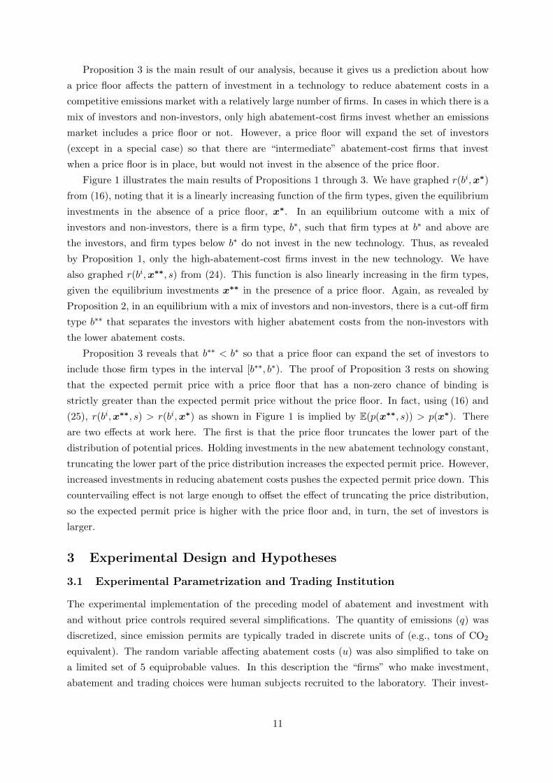
Proposition 3 is the main result of our analysis, because it gives us a prediction about how
a price floor affects the pattern of investment in a technology to reduce abatement costs in a
competitive emissions market with a relatively large number of firms. In cases in which there is a
mix of investors and non-investors, only high abatement-cost firms invest whether an emissions
market includes a price floor or not. However, a price floor will expand the set of investors
(except in a special case) so that there are “intermediate” abatement-cost firms that invest
when a price floor is in place, but would not invest in the absence of the price floor.
Figure 1 illustrates the main results of Propositions 1 through 3. We have graphed r(bi,x∗)
from (16), noting that it is a linearly increasing function of the firm types, given the equilibrium
investments in the absence of a price floor, x∗. In an equilibrium outcome with a mix of
investors and non-investors, there is a firm type, b∗, such that firm types at b∗ and above are
the investors, and firm types below b∗ do not invest in the new technology. Thus, as revealed
by Proposition 1, only the high-abatement-cost firms invest in the new technology. We have
also graphed r(bi,x∗∗, s) from (24). This function is also linearly increasing in the firm types,
given the equilibrium investments x∗∗ in the presence of a price floor. Again, as revealed by
Proposition 2, in an equilibrium with a mix of investors and non-investors, there is a cut-off firm
type b∗∗ that separates the investors with higher abatement costs from the non-investors with
the lower abatement costs.
Proposition 3 reveals that b∗∗ < b∗ so that a price floor can expand the set of investors to
include those firm types in the interval [b∗∗, b∗). The proof of Proposition 3 rests on showing
that the expected permit price with a price floor that has a non-zero chance of binding is
strictly greater than the expected permit price without the price floor. In fact, using (16) and
(25), r(bi,x∗∗, s) > r(bi,x∗) as shown in Figure 1 is implied by E(p(x∗∗, s)) > p(x∗). There
are two effects at work here. The first is that the price floor truncates the lower part of the
distribution of potential prices. Holding investments in the new abatement technology constant,
truncating the lower part of the price distribution increases the expected permit price. However,
increased investments in reducing abatement costs pushes the expected permit price down. This
countervailing effect is not large enough to offset the effect of truncating the price distribution,
so the expected permit price is higher with the price floor and, in turn, the set of investors is
larger.
3 Experimental Design and Hypotheses
3.1 Experimental Parametrization and Trading Institution
The experimental implementation of the preceding model of abatement and investment with
and without price controls required several simplifications. The quantity of emissions (q) was
discretized, since emission permits are typically traded in discrete units of (e.g., tons of CO2
equivalent). The random variable affecting abatement costs (u) was also simplified to take on
a limited set of 5 equiprobable values. In this description the “firms” who make investment,
abatement and trading choices were human subjects recruited to the laboratory. Their invest-
11

Figure 1: Impact of Price Floor on Firms’ Investments in Reducing Abatement Costs
ments, abatement and permit trading decisions determined their monetary payments, which
were distributed in cash at the conclusion of each experimental session.
Each market included 8 heterogeneous firms. Although it may seem relatively thin, this
market size is common in laboratory studies and can result in relatively competitive pricing when
trade is organized using continuous double auction rules (Smith, 1982). The double auction
market used in the experiment provides a competitive environment where traders are free to
submit public offers to purchase and sell permits at any prices. Firms could choose whether
to take the buying or selling side of a transaction—a so-called trader setting (Kotani et al.,
2019). Those wishing to buy permits can submit bid prices to buy or accept sellers’ offer prices
in continuous time. Symmetrically, those wishing to sell permits can submit offer prices to sell
or accept buyers’ bid prices at any time.9 This creates a centralized, multilateral negotiation
process that is relatively competitive even with a small number of traders.
Firm heterogeneity arises from differences in bi, which takes on values of 100, 200, . . . , 800
for the 8 different firms. The discrete shift in abatement costs due to cost-reducing investment
is β = 0.252 and parameter is c = 15 for all firms. Abatement cost uncertainty, the motivation
for the implementation of price controls, is modeled through the mean zero random variable
u, which is drawn each period from the set {−40,−20, 0, 20, 40} with all values equally likely.
A total of 184 emission permits are distributed equally to the 8 firms, so that each began the
trading period holding 23 permits. The heterogeneity in abatement costs creates gains from
trading permits. It also leads the investment incentives to differ across firms, as characterized
in Propositions 1 and 2. The firms with the highest bi have the greatest incentive to invest to
reduce costs. The investment cost f was fixed at 200 Experimental Dollars for all firms.
9Throughout the trading period, firms can adjust their offers but new offers must be an improvement overprevious offers. That is, any new buy offers must be higher than the current highest buy offer and any new selloffers must be lower than the current lowest sell offer.
12
3.2 Period Timing and Equilibrium Prices
The experiment employs stationary repetition. This means that firms make similar investment
and trading decisions in a stable environment across 16 consecutive periods with firm type being
fixed.10 Such repetition is commonly employed in market experiments to allow participants to
gain experience and to provide more opportunity for prices to converge to (or at least approach)
equilibrium levels. New random draws occur each period for the variable affecting abatement
costs (u), however, and these draws affect the equilibrium price.11 Therefore, the equilibrium
price is not stationary.
At the start of each period, traders receive fixed revenues and permits. Those firms with
greater abatement costs receive greater revenues to roughly equate the equilibrium distribution
of net profits across firm types. Following this allocation of fixed revenues and permits, traders
make (binary) investment decisions. They make this investment decision in each of the 16 cycles
of stationary repetition, in order to maximize the number of observations collected for this focus
of our study. Consistent with the theoretical model developed in Section 2, this investment
lowers the marginal cost for each unit abated but does not affect the slope of the marginal
abatement cost function. Firms make this decision simultaneously and they never learn the
investment decisions of others. (Individual firms’ marginal abatement costs are always their
own private information.) Firms then learn the realization of the random variable affecting
abatement costs (u).12 Traders’ investment decisions and this realization of u lead to a new
abatement cost profile across traders of each type. Equilibrium permit prices therefore depend
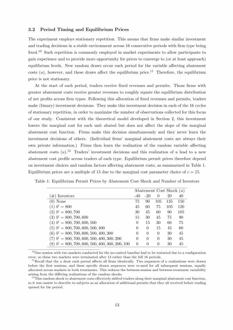
on investment choices and random factors affecting abatement costs, as summarized in Table 1.
Equilibrium prices are a multiple of 15 due to the marginal cost parameter choice of c = 15.
Table 1: Equilibrium Permit Prices by Abatement Cost Shock and Number of Investors
Abatement Cost Shock (u)(#) Investors -40 -20 0 20 40
(0) None 75 90 105 135 150(1) bi = 800 45 60 75 105 120(2) bi = 800, 700 30 45 60 90 105(3) bi = 800, 700, 600 15 30 45 75 90(4) bi = 800, 700, 600, 500 0 15 30 60 75(5) bi = 800, 700, 600, 500, 400 0 0 15 45 60(6) bi = 800, 700, 600, 500, 400, 300 0 0 0 30 45(7) bi = 800, 700, 600, 500, 400, 300, 200 0 0 0 30 45(8) bi = 800, 700, 600, 500, 400, 300, 200, 100 0 0 0 30 45
10One session with two markets conducted for the no-control baseline had to be restarted due to a configurationerror, so these two markets were terminated after 13 rather than the full 16 periods.
11Recall that the u draw each period affects all firms identically. Two sequences of u realizations were drawnbefore the first sessions, and these specific drawn sequences were re-used for all subsequent sessions, equallyallocated across markets in both treatments. This reduces the between-session and between-treatment variabilityarising from the differing realizations of the random shocks.
12This random shock to abatement costs effectively shifted traders along their marginal abatement cost function,so it was easiest to describe to subjects as an allocation of additional permits that they all received before tradingopened for the period.
13
Trading periods lasted for 3 minutes until period 6, when the length was reduced to 2 minutes.
Prior to these 16 periods of stationary repetition, subjects first participated in 8 (paid) training
periods to familiarize them with the mechanics of continuous double auction trading through the
computer interface. These training periods also included an investment stage, but they employed
different abatement cost parameters and permit allocations so that transaction prices were very
different from the prices in the main experiment.13 The training periods never employed price
controls. The training periods and the main periods each began with one practice period without
financial stakes.
3.3 Price Floor
The treatment variable in the experiment is the price floor, imposed for this chosen parameter-
ization at 70. This particular level of 70 is not set at an optimal (or second-best) level, which
is not defined as we leave the marginal environmental damages unspecified. To implement the
floor no offers or transactions were allowed at prices below 70; they were automatically disal-
lowed by the market software. Obviously, this led to an excess supply of permits at the floor
price when the floor was binding. Consistent with the implementation of hard price floors in
emissions permit markets in practice, firms wishing to sell these excess permits were able to sell
them to “the computer,” analogous to the regulator standing ready to buy excess permits at
the floor. In order to create a marginal incentive to sell to actual traders wishing to buy at the
floor during the trading period, the computer made these purchases at the close of trading and
at a price of 69. Firms decided how many permits to sell at this price floor.14
3.4 Laboratory Procedures and Power Analysis
In order to determine subjects’ understanding of the investment decisions and different ways of
implementing the price floor, we initially ran 3 pilot sessions.15 These pilots generated realized
effect sizes and variance estimates that were used in a power analysis to design the main exper-
iment. These power calculations led to the conclusion that 11 markets would be sufficient to
detect a difference in investment rates with power 0.80 and significance level 0.05. The power
analysis also prescribed a greater allocation of markets to the price control condition due to a
higher variance observed in this treatment for the pilot sessions.
We therefore collected data from a total of 11 markets, with the price floor treatment imple-
mented in 6 markets and the no-control baseline in the other 5 markets. Each market included 8
traders as described above. The subjects were all undergraduate students at Purdue University,
recruited from a database of approximately 3,000 volunteers drawn across a wide range of aca-
13Equilibrium prices in the training periods ranged between 120 and 300, and had virtually no overlap with theprices shown in Table 1 for the main periods.
14Firms could sell as many permits at the floor as they wished. The software implemented a decision aidon-screen, which indicated the number of profitable permits they could sell; i.e., the number of currently heldpermits that correspond to avoided abatement costs lower than the price floor.
15These pilot sessions led us to add the 8 training periods described earlier, so that subjects did not have tolearn the mechanics of trading at the same time they learned how permit prices depend on investment decisionsand investment incentives depend on prices and the price floor.
14
demic disciplines and randomly allocated to treatment conditions using ORSEE (Greiner, 2015).
The z-Tree program (Fischbacher, 2007) was used for the implementation of the experiment. For
the purpose of maintaining as much experimental control as possible, we used neutral framing
in the experiment and did not refer to the specific environmental economics setting explicitly,
since environmental framing could affect subjects’ preferences differently (Cason and Raymond,
2011). In particular, tradable emission permits were referred to as “coupons,” and abatement
and marginal abatement cost were referred to as “production” and “production costs,” respec-
tively that firms could avoid by holding more coupons. Details are provided in the written
instructions given to subjects (see Appendix B).
Each session lasted about 2 hours and after each session earnings were paid out privately
in cash at a pre-announced conversion rate from the Experimental Dollars earned across all
(non-practice) periods. On average, subjects earned $33.47 per person.
3.5 Testable Hypotheses
The implications of the theoretical model and corresponding experimental design allow us to
test several hypotheses. We first consider the impact of price controls on investment levels. As
described earlier, all eight firms make their investment choice simultaneously. The competitive
equilibrium permit prices shown in Table 1 indicate that the price floor of 70 is often binding.
This was a deliberate design choice so that the differences in investment incentives would be
large enough to substantially change the number of equilibrium investors. As noted earlier,
analysis of costs and prices in large emissions trading markets such as California’s GHG market
has concluded that market prices are very likely to be limited by administrative price floors or
ceilings (Borenstein et al., 2019).
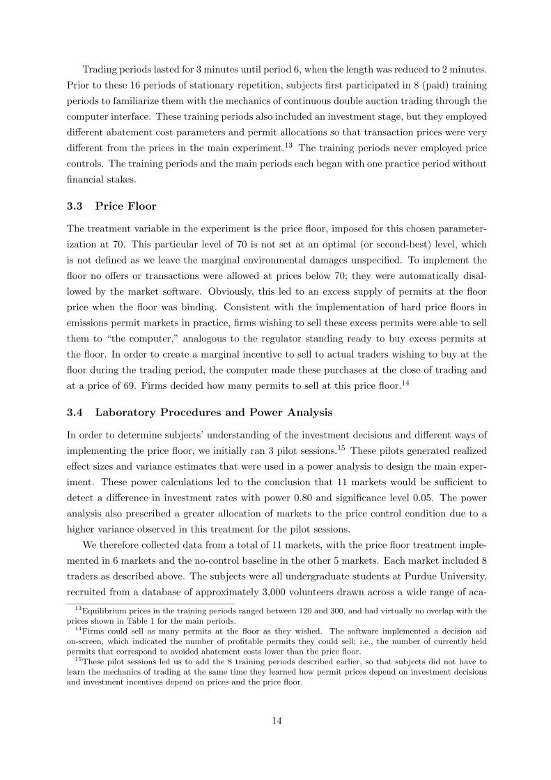
Table 2: Increase in Expected Profits from Investing in Abatement Cost Reductions, Gross ofInvestment Cost
Firm Investor Type No Price Floor Price Floor = 70
bi = 800 1788 1706bi = 700 1077 1105bi = 600 720 834bi = 500 408 600bi = 400 192 492bi = 300 48 350bi = 200 45 210bi = 100 30 140
Notes: Amounts shown in experimental dollars, based on equiprob-able likelihood of the 5 abatement cost shocks. Entries in boldindicate firms with incentive to invest for the investment cost usedin experiment (200).
Those firms with the highest abatement costs have the greatest incentive to invest to reduce
their abatement costs, as indicated by the cutoff firm types as derived in Propositions 1 and 2.
For the experimental parameterization, the highest cost types (i.e., those with the greatest bi)
15
always have the incentive to invest and the lowest cost types never have the incentive to invest,
regardless whether a price floor exists. The price floor affects the investment decision of the
intermediate-cost firms. Table 2 shows that in equilibrium 4 firms have an incentive to invest
without a price floor but 7 firms would invest with the price floor. This leads to our primary
hypothesis in connection to Proposition 3.
Hypothesis 1 (Investment): In a competitive permit market,
(a) A price floor increases the total number of firms investing in reducing their abatement
costs; and
(b) The change in investment frequency is greatest for firms with intermediate abatement
costs.
The investment incentives arise through the price implications on the permit market, so a
necessary condition for support of Hypothesis 1 is a correlation between prices and abatement
shocks and investment. This is summarized by the second hypothesis:
Hypothesis 2 (Prices): Emission permit prices are
(a) lower on average without the price floor than with the price floor in place;
(b) lower in periods with favorable shocks that lower abatement costs for all firms; and,
(c) lower in periods in which a greater number of firms invest in reducing abatement costs.
Hypothesis 2(a) is based on the primary implication of a price floor that has a non-zero
chance of binding, since it truncates the lower part of the distribution of potential prices. For
the other two parts of this hypothesis, Table 1 illustrates the specific amounts in equilibrium that
prices change due to investment and cost shocks without the price floor. Of course, these price
differences are limited by the price floor when it is imposed. When investment is sufficiently
high or the abatement cost shock is favorable, the price floor will bind and parts (b) and (c) of
Hypothesis 2 will not apply.
4 Experimental Results
This section is divided into two subsections, corresponding to the two hypotheses regarding
cost-reducing investment and emission permit prices.
4.1 Cost-Reducing Investment
The price floor theoretically increases the number of investing firms because it helps to preserve
the benefits of lower abatement costs even when favorable cost shocks cause prices to fall to
low levels. For the parameters used in the experiment, 7 of the 8 firms can profitably invest
in the price floor treatment, while only 4 firms can invest profitably without the price floor.
16
0
1
2
3
4
5
6
7
0 2 4 6 8 10 12 14 16
Ave
rage
Num
ber
of I
nves
tors
(8
max
imum
)
Period
Price Floor
No Control
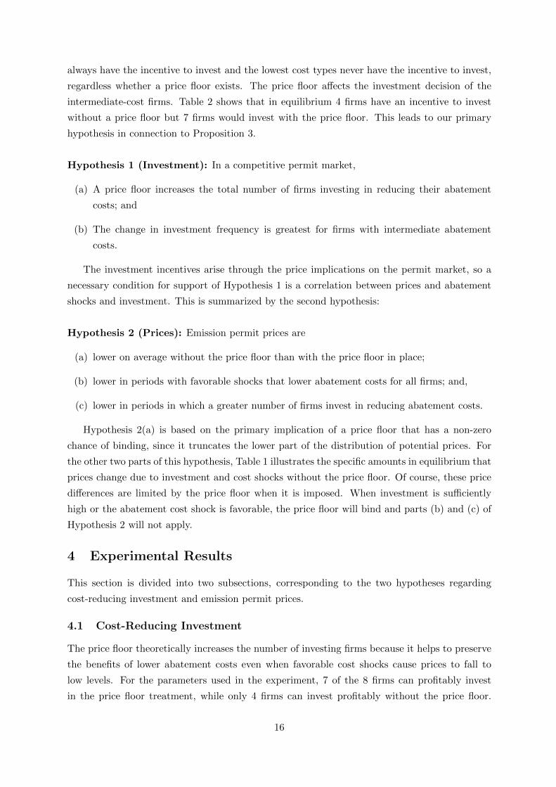
Figure 2: Mean Number of Investors, by Period
Figure 2 displays the average number of investing firms across periods, pooling over all 11
markets. Although the difference in the investment frequency is similar for the first few periods,
a persistent gap across treatments emerges over time. The difference is in the direction predicted
in Hypothesis 1(a).
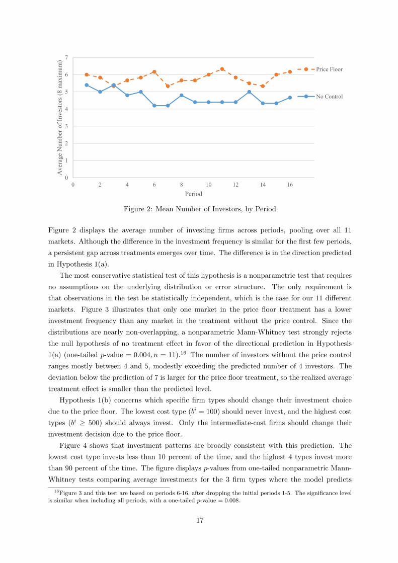
The most conservative statistical test of this hypothesis is a nonparametric test that requires
no assumptions on the underlying distribution or error structure. The only requirement is
that observations in the test be statistically independent, which is the case for our 11 different
markets. Figure 3 illustrates that only one market in the price floor treatment has a lower
investment frequency than any market in the treatment without the price control. Since the
distributions are nearly non-overlapping, a nonparametric Mann-Whitney test strongly rejects
the null hypothesis of no treatment effect in favor of the directional prediction in Hypothesis
1(a) (one-tailed p-value = 0.004, n = 11).16 The number of investors without the price control
ranges mostly between 4 and 5, modestly exceeding the predicted number of 4 investors. The
deviation below the prediction of 7 is larger for the price floor treatment, so the realized average
treatment effect is smaller than the predicted level.
Hypothesis 1(b) concerns which specific firm types should change their investment choice
due to the price floor. The lowest cost type (bi = 100) should never invest, and the highest cost
types (bi ≥ 500) should always invest. Only the intermediate-cost firms should change their
investment decision due to the price floor.
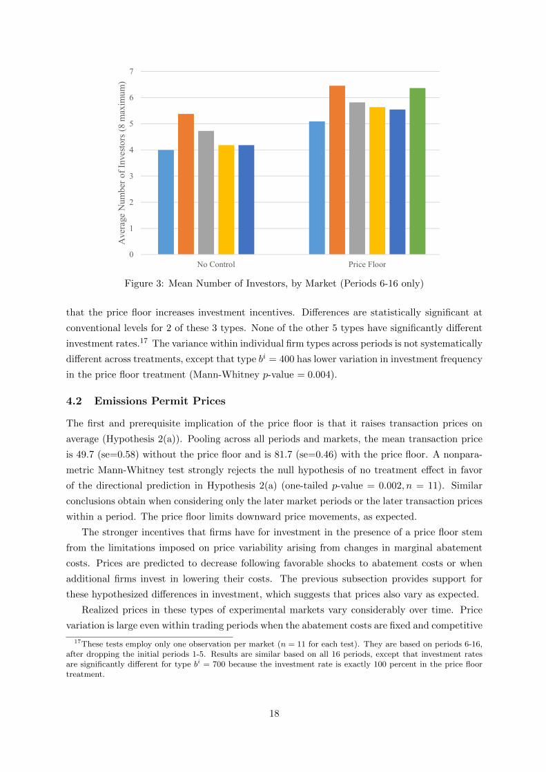
Figure 4 shows that investment patterns are broadly consistent with this prediction. The
lowest cost type invests less than 10 percent of the time, and the highest 4 types invest more
than 90 percent of the time. The figure displays p-values from one-tailed nonparametric Mann-
Whitney tests comparing average investments for the 3 firm types where the model predicts
16Figure 3 and this test are based on periods 6-16, after dropping the initial periods 1-5. The significance levelis similar when including all periods, with a one-tailed p-value = 0.008.
17
0
1
2
3
4
5
6
7
No Control Price Floor
Ave
rage
Num
ber
of I
nves
tors
(8
max
imum
)
Figure 3: Mean Number of Investors, by Market (Periods 6-16 only)
that the price floor increases investment incentives. Differences are statistically significant at
conventional levels for 2 of these 3 types. None of the other 5 types have significantly different
investment rates.17 The variance within individual firm types across periods is not systematically
different across treatments, except that type bi = 400 has lower variation in investment frequency
in the price floor treatment (Mann-Whitney p-value = 0.004).
4.2 Emissions Permit Prices
The first and prerequisite implication of the price floor is that it raises transaction prices on
average (Hypothesis 2(a)). Pooling across all periods and markets, the mean transaction price
is 49.7 (se=0.58) without the price floor and is 81.7 (se=0.46) with the price floor. A nonpara-
metric Mann-Whitney test strongly rejects the null hypothesis of no treatment effect in favor
of the directional prediction in Hypothesis 2(a) (one-tailed p-value = 0.002, n = 11). Similar
conclusions obtain when considering only the later market periods or the later transaction prices
within a period. The price floor limits downward price movements, as expected.
The stronger incentives that firms have for investment in the presence of a price floor stem
from the limitations imposed on price variability arising from changes in marginal abatement
costs. Prices are predicted to decrease following favorable shocks to abatement costs or when
additional firms invest in lowering their costs. The previous subsection provides support for
these hypothesized differences in investment, which suggests that prices also vary as expected.
Realized prices in these types of experimental markets vary considerably over time. Price
variation is large even within trading periods when the abatement costs are fixed and competitive
17These tests employ only one observation per market (n = 11 for each test). They are based on periods 6-16,after dropping the initial periods 1-5. Results are similar based on all 16 periods, except that investment ratesare significantly different for type bi = 700 because the investment rate is exactly 100 percent in the price floortreatment.
18
0
0.1
0.2
0.3
0.4
0.5
0.6
0.7
0.8
0.9
1
0 100 200 300 400 500 600 700 800
Ave
rage
Inv
estm
ent F
requ
ency
Firm Cost Type
Price Floor
No Control
0.002
0.219
0.048
Figure 4: Mean Investment Rate, Across Firm Types (Periods 6-16 only). P -values shown forkey firm types bi = 200, 300, 400 where Hypothesis 1(b) predicts a significant difference.
equilibrium prices are unchanging. Previous experiments using this continuous double auction
trading institution show that prices converge eventually when the competitive equilibrium is
stable across periods. Not surprisingly, however, prices do not converge to equilibrium in an
environment like this one where prices change randomly due to cost shocks and through firm-
specific, cost-reducing investments.
Table 1 above indicates that equilibrium prices typically decline by 15 experimental dollars
for each additional shift down to a more favorable cost shock, or when an additional firm invests
in cost reduction.18 We summarized these directional predictions above in Hypothesis 2. These
price reductions are limited by the zero lower bound on prices, or limited by the price floor (70).
Due to their already low abatement costs, cost reductions by firm types bi ≤ 200 do not impact
equilibrium prices.
The early trades in each period are especially volatile and often occur far from equilibrium
levels. As trades occur within a period, however, the market conveys information about under-
lying abatement costs (which are, recall, firms’ private information). The later trading prices
therefore reveal more about market conditions and become closer to equilibrium levels. For this
reason we focus our analysis of the transaction prices to the later trades that occur each period.
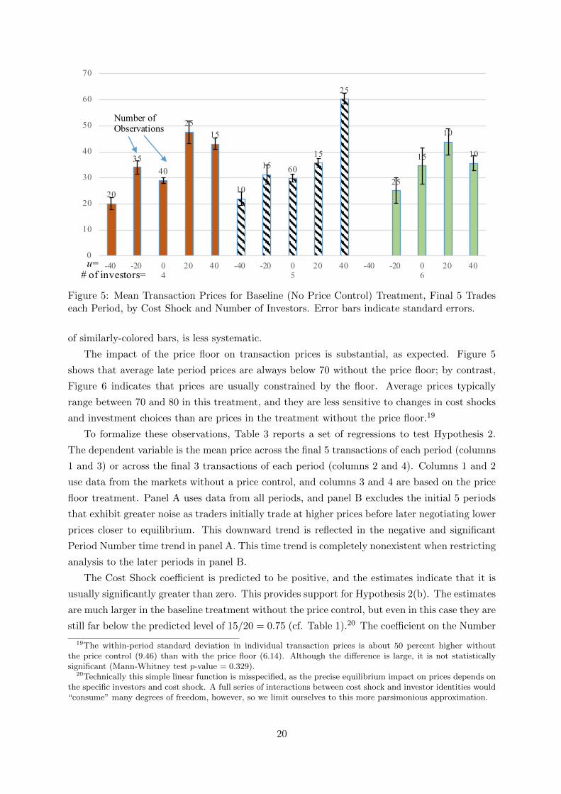
Figure 5 displays the mean transaction prices for the baseline treatment without a price
control, considering only the final 5 trades each period. Each bar corresponds to a different
combination of a number of investors and abatement cost shock. Only the most common number
of investors (4, 5 and 6) are displayed. Although in equilibrium prices should be 0 or 15 in nearly
half of these cases (cf. rows (4) through (6) of Table 1), the displayed average prices are always
20 or greater. Average prices nevertheless tend to rise, as predicted, for more unfavorable cost
shocks. The decrease in prices due to an increase in investment, moving rightward across blocks
18The price difference is larger (30) between the 0 and 20 cost shock due to rounding.
19
20
3540
2515
10
15 60
15
25
25
15
10
10
0
10
20
30
40
50
60
70
-40 -20 04
20 40 -40 -20 05
20 40 -40 -20 06
20 40u=# of investors=
Number of Observations
Figure 5: Mean Transaction Prices for Baseline (No Price Control) Treatment, Final 5 Tradeseach Period, by Cost Shock and Number of Investors. Error bars indicate standard errors.
of similarly-colored bars, is less systematic.
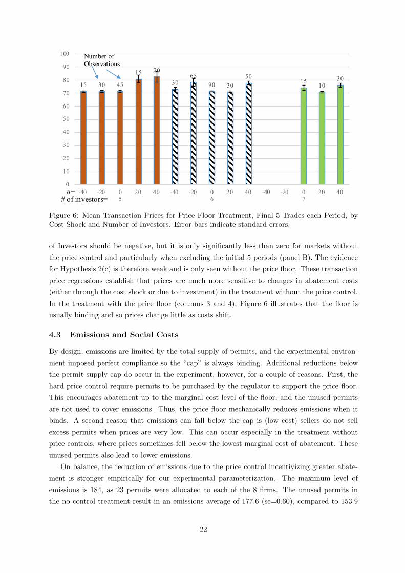
The impact of the price floor on transaction prices is substantial, as expected. Figure 5
shows that average late period prices are always below 70 without the price floor; by contrast,
Figure 6 indicates that prices are usually constrained by the floor. Average prices typically
range between 70 and 80 in this treatment, and they are less sensitive to changes in cost shocks
and investment choices than are prices in the treatment without the price floor.19
To formalize these observations, Table 3 reports a set of regressions to test Hypothesis 2.
The dependent variable is the mean price across the final 5 transactions of each period (columns
1 and 3) or across the final 3 transactions of each period (columns 2 and 4). Columns 1 and 2
use data from the markets without a price control, and columns 3 and 4 are based on the price
floor treatment. Panel A uses data from all periods, and panel B excludes the initial 5 periods
that exhibit greater noise as traders initially trade at higher prices before later negotiating lower
prices closer to equilibrium. This downward trend is reflected in the negative and significant
Period Number time trend in panel A. This time trend is completely nonexistent when restricting
analysis to the later periods in panel B.
The Cost Shock coefficient is predicted to be positive, and the estimates indicate that it is
usually significantly greater than zero. This provides support for Hypothesis 2(b). The estimates
are much larger in the baseline treatment without the price control, but even in this case they are
still far below the predicted level of 15/20 = 0.75 (cf. Table 1).20 The coefficient on the Number
19The within-period standard deviation in individual transaction prices is about 50 percent higher withoutthe price control (9.46) than with the price floor (6.14). Although the difference is large, it is not statisticallysignificant (Mann-Whitney test p-value = 0.329).
20Technically this simple linear function is misspecified, as the precise equilibrium impact on prices depends onthe specific investors and cost shock. A full series of interactions between cost shock and investor identities would“consume” many degrees of freedom, however, so we limit ourselves to this more parsimonious approximation.
20
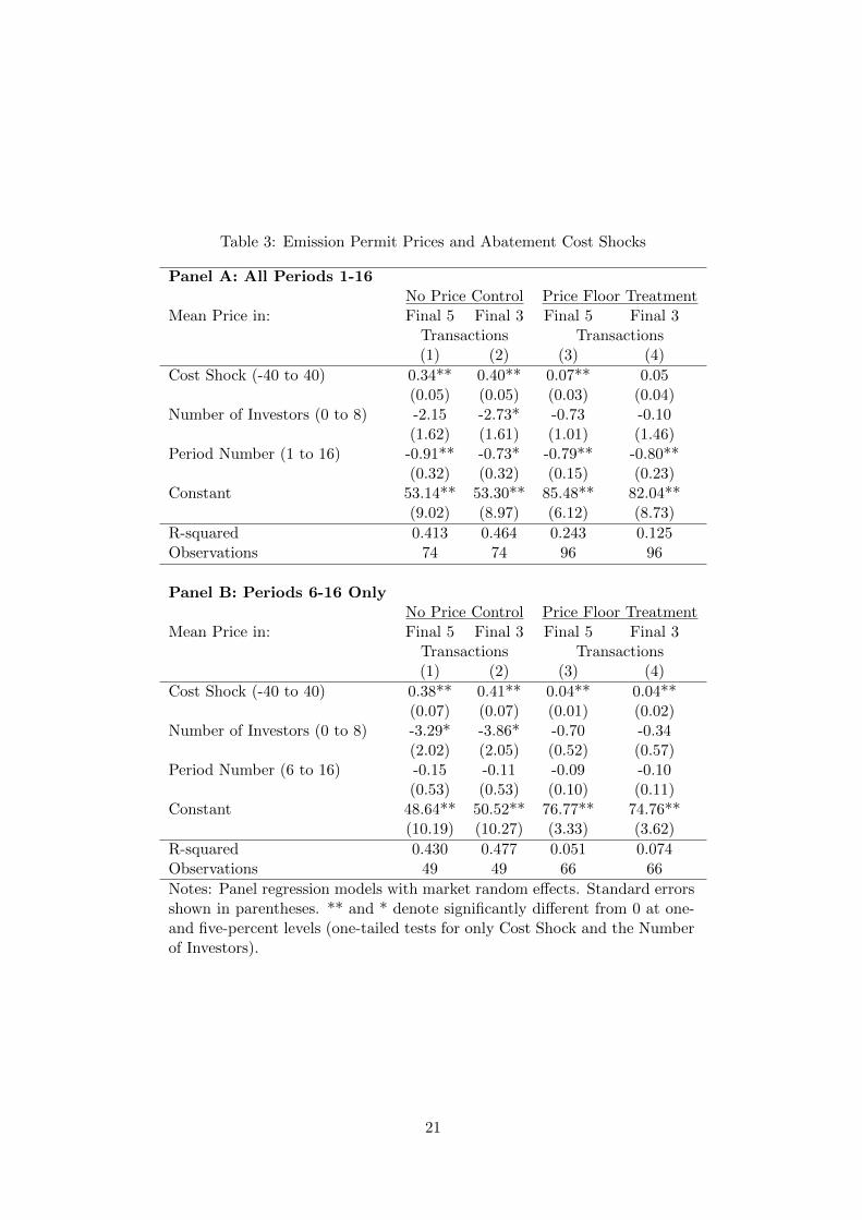
Table 3: Emission Permit Prices and Abatement Cost Shocks
Panel A: All Periods 1-16No Price Control Price Floor Treatment
Mean Price in: Final 5 Final 3 Final 5 Final 3Transactions Transactions(1) (2) (3) (4)
Cost Shock (-40 to 40) 0.34** 0.40** 0.07** 0.05(0.05) (0.05) (0.03) (0.04)
Number of Investors (0 to 8) -2.15 -2.73* -0.73 -0.10(1.62) (1.61) (1.01) (1.46)
Period Number (1 to 16) -0.91** -0.73* -0.79** -0.80**(0.32) (0.32) (0.15) (0.23)
Constant 53.14** 53.30** 85.48** 82.04**(9.02) (8.97) (6.12) (8.73)
R-squared 0.413 0.464 0.243 0.125Observations 74 74 96 96
Panel B: Periods 6-16 OnlyNo Price Control Price Floor Treatment
Mean Price in: Final 5 Final 3 Final 5 Final 3Transactions Transactions(1) (2) (3) (4)
Cost Shock (-40 to 40) 0.38** 0.41** 0.04** 0.04**(0.07) (0.07) (0.01) (0.02)
Number of Investors (0 to 8) -3.29* -3.86* -0.70 -0.34(2.02) (2.05) (0.52) (0.57)
Period Number (6 to 16) -0.15 -0.11 -0.09 -0.10(0.53) (0.53) (0.10) (0.11)
Constant 48.64** 50.52** 76.77** 74.76**(10.19) (10.27) (3.33) (3.62)
R-squared 0.430 0.477 0.051 0.074Observations 49 49 66 66
Notes: Panel regression models with market random effects. Standard errorsshown in parentheses. ** and * denote significantly different from 0 at one-and five-percent levels (one-tailed tests for only Cost Shock and the Numberof Investors).
21
15 30 45
15 20
3065
90 3050
1510
30
0
10
20
30
40
50
60
70
80
90
100
-40 -20 05
20 40 -40 -20 06
20 40 -40 -20 07
20 40u=# of investors=
Number of Observations
Figure 6: Mean Transaction Prices for Price Floor Treatment, Final 5 Trades each Period, byCost Shock and Number of Investors. Error bars indicate standard errors.
of Investors should be negative, but it is only significantly less than zero for markets without
the price control and particularly when excluding the initial 5 periods (panel B). The evidence
for Hypothesis 2(c) is therefore weak and is only seen without the price floor. These transaction
price regressions establish that prices are much more sensitive to changes in abatement costs
(either through the cost shock or due to investment) in the treatment without the price control.
In the treatment with the price floor (columns 3 and 4), Figure 6 illustrates that the floor is
usually binding and so prices change little as costs shift.
4.3 Emissions and Social Costs
By design, emissions are limited by the total supply of permits, and the experimental environ-
ment imposed perfect compliance so the “cap” is always binding. Additional reductions below
the permit supply cap do occur in the experiment, however, for a couple of reasons. First, the
hard price control require permits to be purchased by the regulator to support the price floor.
This encourages abatement up to the marginal cost level of the floor, and the unused permits
are not used to cover emissions. Thus, the price floor mechanically reduces emissions when it
binds. A second reason that emissions can fall below the cap is (low cost) sellers do not sell
excess permits when prices are very low. This can occur especially in the treatment without
price controls, where prices sometimes fell below the lowest marginal cost of abatement. These
unused permits also lead to lower emissions.
On balance, the reduction of emissions due to the price control incentivizing greater abate-
ment is stronger empirically for our experimental parameterization. The maximum level of
emissions is 184, as 23 permits were allocated to each of the 8 firms. The unused permits in
the no control treatment result in an emissions average of 177.6 (se=0.60), compared to 153.9
22
(se=1.11) for the price floor treatment. This difference is highly significant (Mann-Whitney
p-value = 0.004). The price floor therefore leads to greater investment, lower price volatility,
more abatement and less emissions.
However, we cannot say whether the additional investments in abatement costs and the
reduction in emissions results in a welfare gain unless we are willing to specify an ad hoc
marginal damage function. We can, however, derive a range of marginal damages that would
imply that the price floor in our experiments lowers expected social costs. To do so, suppose
that marginal damage is a constant, d, which is close to reality if we are considering carbon
emissions (Pizer, 2002). Let observed aggregate emissions with the price floor and without the
price floor be Qs and Qns, respectively. Likewise, let As and Ans denote the firms’ aggregate
abatement costs plus their aggregate investments in reducing their abatement costs, with and
without the price floor. Finally, define expected social costs to be SCk = Ak +dQk, k = {s, ns}.We do not include government’s expenditure on buying unused permits under the price floor,
because this is a simple transfer from one part of society to another. However, there is likely
a cost to generate these funds in the first place, so we acknowledge that a fuller accounting of
the social costs would include the deadweight cost of an additional dollar of government revenue
times the government’s expenditure on buying permits.
Calculate SCns − SCs = Ans −As + d(Qns −Qs). Given Qns −Qs > 0 as we observe in our
experiments, there exists a cut-off value of d,
d =As −Ans
Qns −Qs,
for which d > (<) d implies SCns > (<)SCs. That is, if actual marginal damage is greater than
(less than) d then the price floor reduces (increases) expected social costs.
We noted above that over all 16 periods of our experiments the mean observed levels of
aggregate emissions are Qs = 153.9 and Qns = 177.6. The mean observed levels of aggregate
abatement costs plus investment costs are As = 2864.4 and Ans = 1905.7. Thus, the firms’ costs
of reducing their emissions under the price floor increased despite the significant increase in
investments to reduce their abatement costs. With these emissions and cost values, d = 40.45.
This implies that the price floor in our experiments would lead to an increase in social welfare
if marginal damage exceeds this value. (This value is only a bit higher at 43.05 if we consider
only periods 6-16.) Note that this value is below our price floor of 70. Actual price floors in
existing markets tend to be well below estimates of the marginal damage from greenhouse gas
emissions. If that was also true in our experimental markets then we would conclude that the
hard price floor we consider leads to lower social costs.
One final note is warranted. The cut-off value d would be higher if we included the social
costs of the government’s purchases of unused permits under the price floor. Typical corrections
for the marginal excess burden of taxation (i.e., the deadweight costs of raising an additional
dollar of government revenue) are less than 50 percent (Bos et al., 2019). Even if we assumed a
100 percent correction, d would only increase from 40.45 to 41.72.
23
5 Conclusion
This paper develops a theoretical model that identifies firms’ investment incentives in abatement
technology for emissions trading markets characterized by cost uncertainty and regulated by
price floors. The establishment of a price floor is pivotal in mitigating permit price uncertainty
and limits market prices from becoming too low, which impedes investment and undermines the
dynamic efficiency of markets. A price floor acts as an implicit subsidy for firms, as it increases
the expected benefits from investment in lower abatement cost technology.
In a model featuring abatement cost uncertainty and a set of heterogeneous firms that interact
in a competitive emissions trading market, our model reveals that, compared to an unregulated
market, investment incentives are stronger when price floors are in place. In a market with a mix
of investors and non-investors, the price floor expands the number of investors in equilibrium.
This key result is also supported empirically in a laboratory market experiment, which also
indicates how transaction prices are sensitive to cost shocks and the number of investors. The
policy lesson to be drawn from this is that additional investments in cost-saving technologies
can be achieved through the implementation of a price floor; ultimately, this has the potential
to promote innovation and development of advanced abatement technology.
The experiment, of course, must impose a specific numerical parameterization for the labo-
ratory market, and so we do not claim to provide broad empirical conclusions that can apply
generally to the wide range of current and potential markets for emissions permits in the field.
The experiment’s structure is guided closely by the theoretical model, however, and we believe
it captures the important economic forces that cause price floors to promote abatement cost-
reducing investment. The identification of clear causal channels with direct theoretical support
helps promote confidence in external validity. When the price floor has a positive probability
of binding, which is commonly the case for many emissions markets in practice (discussed in
the Introduction), investment is likely to increase when the market is composed of a mixture of
heterogeneous firms who invest at different levels.
Finally, for the purpose of the experiment we studied the effect of a price floor in a single
emissions trading market in isolation without consideration of endogenous policy choices that
could arise in the field. Actual field markets may be subject to multiple interacting policy
levers, which may shape investment decisions differently. For instance, price floors may differ
across nations for political economy reasons. More specifically, individual countries in the EU
ETS with more ambitious climate targets may have a preference for enhancing market signals
through implementing a relatively high price floor domestically. As a result, asymmetric price
controls across nations may undermine the harmonization of international emissions trading
markets. However, Newbery et al. (2019) argue that domestic and EU-wide price floors could
be mutually enhancing. Either way it is important to assess how price floors shape and affect the
functioning of emissions markets. While our paper has shed light on the impacts of price floors
on investments in abatement technology, future research could incorporate adjusting permit
supply, for instance through the lens of the Market Stability Reserve in the EU ETS.
24
Appendix A: Model Derivations and Proofs
Derivation of Equation (12)
Start with
∆ci(x, u) = ci(xi = 1, x−i, u)− ci(xi = 0, x−i, u).
To conserve notation, let p(1) = p(xi = 1, x−i) and p(0) = p(xi = 0, x−i). Moreover, define
∆ip = (p(1) + u)− (p(0) + u). Then,
∆ci(x, u) = (p(1) + u)
(bi(1− β) + u
c− p(1) + u
2c− li0
)− (p(0) + u)
(bi + u
c− p(0) + u
2c− li0
)=∆ip
(bi
c− li0 −
p(1) + p(0)
2c
)− (p(1) + u)biβ
c
Since p(1) = p(0) + ∆ip,
∆ci(x, u) = ∆ip
(bi − p(0)
c− li0 −
∆ip
2c
)− (p(1) + u)biβ
c,
which is equation (12).
Proposition 1
Proof. Note that r(bi,x∗), given by (16), is linearly increasing in bi. Therefore, b∗ defined by(17) is unique. Moreover, f ≤ r(bi,x∗) and xi = 1 for firm types bi ≥ b∗, and f > r(bi,x∗)and xi = 0 for firm types bi < b∗. If b∗ ∈ [bmin, bmax], then f ≤ r(bi,x∗) and xi = 1 for firmtypes bi ∈ [b∗, bmax], and f > r(bi,x∗) and xi = 0 for firm types bi ∈ [bmin, b∗). If b∗ > bmax,then f < r(bi,x∗) and xi = 1 for all firms; if b∗ < bmin, then f > r(bi,x∗) and xi = 0 for allfirms.
Proposition 2
Proof. Proposition 2 is proved in the same way as Proposition 1. First note that r(bi,x∗∗, s),given by (24), is linearly increasing in bi. Therefore, b∗∗ defined by (26) is unique. Moreover,f ≤ r(bi,x∗∗, s) and xi = 1 for firm types bi ≥ b∗∗, and f > r(bi,x∗∗, s) and xi = 0 for firm typesbi < b∗∗. If b∗∗ ∈ [bmin, bmax], then f ≤ r(bi,x∗∗, s) and xi = 1 for firm types bi ∈ [b∗∗, bmax], andf > r(bi,x∗∗, s) and xi = 0 for firm types bi ∈ [bmin, b∗∗). If b∗∗ > bmax, then f < r(bi,x∗∗, s)and xi = 1 for all firms; if b∗∗ < bmin, then f > r(bi,x∗∗, s) and xi = 0 for all firms.
Proposition 3
Proof. To prove part (1) of the proposition, first note that (17) and (26) imply
b∗p(x∗) = b∗∗E(p(x∗∗, s)). (27)
Subtracting b∗∗p(x∗) from both sides of (27) allows us to obtain
sgn(b∗ − b∗∗) = sgn {E(p(x∗∗, s))− p(x∗)} . (28)
Thus, what happens to the equilibrium set of investors when a price floor is imposed dependson what happens to the expected permit price.
25

We have
E(p(x∗∗, s)) =
∫ us∗∗
usg(u)du+
∫ u
us∗∗(p(x∗∗) + u)g(u)du. (29)
From (18), s = p(x∗∗) + us∗∗. Substitute this into (29) to obtain
E(p(x∗∗, s)) = p(x∗∗) + us∗∗∫ us∗∗
usg(u)du+
∫ u
us∗∗ug(u)du. (30)
Note that p(x∗) can be written as
p(x∗) =
∫ us∗∗
u(p(x∗) + u)g(u)du+
∫ u
us∗∗(p(x∗) + u)g(u)du.
= p(x∗) +
∫ us∗∗
uug(u)du+
∫ u
us∗∗ug(u)du. (31)
Subtract (31) from (30) to obtain
E(p(x∗∗, s)− p(x∗) = p(x∗∗)− p(x∗) +
∫ us∗∗
u(us∗∗ − u)g(u)du. (32)
Toward signing (32), first note that our assumption that there is a strictly positive probabilitythat the price floor will bind implies us∗∗ > u, which in turn implies∫ us∗∗
u(us∗∗ − u)g(u)du > 0. (33)
To determine the relationship between p(x∗∗) and p(x∗), use the price equation (6) to write
p(x∗∗)− p(x∗) =
∑nj=1 b
j(1− βxj∗∗)− cLn
−∑n
j=1 bj(1− βxj∗)− cL
n
=
(1
n
) n∑j=1
bjβxj∗ −n∑
j=1
bjβxj∗∗
, (34)
where xj∗∗ and xj∗ are equilibrium investment choices by firm j, with and without a price floor,respectively. Given bjβ > 0 for all firm types, (34) implies
sgn (p(x∗∗)− p(x∗)) = sgn
n∑j=1
xj∗ −n∑
j=1
xj∗∗
. (35)
Let the equilibrium set of investors in the absence of a price floor be I∗ and let the set of investorswith the price floor be I∗∗. In addition, let |I∗| and |I∗∗| denote the cardinality (i.e., number ofelements) of I∗ and I∗∗, respectively. Note that
|I∗| =n∑
j=1
xj∗ and |I∗∗| =n∑
j=1
xj∗∗.
Then,sgn (p(x∗∗)− p(x∗)) = sgn (|I∗| − |I∗∗|) . (36)
26
Toward a contradiction of b∗ > b∗∗ in the Proposition, suppose instead that b∗ ≤ b∗∗. From(28), this would imply E(p(x∗∗, s)) − p(x∗) ≤ 0. However, from (32) and (33), E(p(x∗∗, s)) −p(x∗) ≤ 0 requires p(x∗∗)−p(x∗) < 0, which from (36) implies |I∗| < |I∗∗|. However, |I∗| < |I∗∗|requires b∗ > b∗∗, which contradicts b∗ ≤ b∗∗. Since b∗ � b∗∗, we have b∗ > b∗∗.
Part (2) of Proposition 3 follows directly from Propositions 1, 2 and part (1) of Proposition3.
Appendix B: Experiment Instructions –Not Intended for Publication
Note: Text that is shown only for price floor treatment is displayed in bold font.
5.1 General
This is an experiment in the economics of decision making. The instructions are simple and if
you follow them carefully and make good decisions you will earn money that will be paid to you
privately in cash. All earnings on your computer screens are in Experimental Dollars. These
Experimental Dollars will be converted to real Dollars at the end of the experiment, at a rate
of 1000 Experimental Dollars = 1 real Dollar. Notice that the more Experimental Dollars you
earn, the more cash that you receive at the end of the experiment. Everyone will also receive a
fixed participation payment of $5 that will be added to this total.
At your seat you have a sheet labeled Personal Record Sheet, which will help you keep track
of how your decisions impact your earnings. You also have a sheet indicating your trading values
for coupons (costs avoided when purchasing or additional costs incurred by selling). You are
not to reveal this information to anyone. It is your own private information.
In each period you will produce units of a good. For every unit of the good that you produce,
you will incur a production cost which will take away from your earnings. In order to avoid
these costs, you may wish to purchase “coupons.” Each coupon allows you to produce 1 less
unit of the good, and avoid those production costs.
At the beginning of each period you will receive cash in the form of a Fixed Period Revenue,
which will be labelled as Cash on your investment and trading screens. You will also have the
opportunity to make an investment which can lower your production costs. Afterwards everyone
will receive a small number of additional coupons, with the amount determined randomly. There
will then be a time for you to sell or purchase coupons to and from other participants. At the
end of each period you will pay your production costs, which will depend on how many coupons
you hold. Your earnings each period are determined as follows:
Earnings = Fixed Period Revenue – Total Production Costs – Investment Cost (if any)
+ Sale Proceeds from Selling Coupons – Amount Spent when Buying Coupons.
Your Fixed Period Revenue does not depend on any actions you take, and does not change
throughout the experiment. (In fact, it is already written on your Personal Record Sheet.) You
will receive this revenue at the beginning of each period so that you have cash available with
which to trade.
27
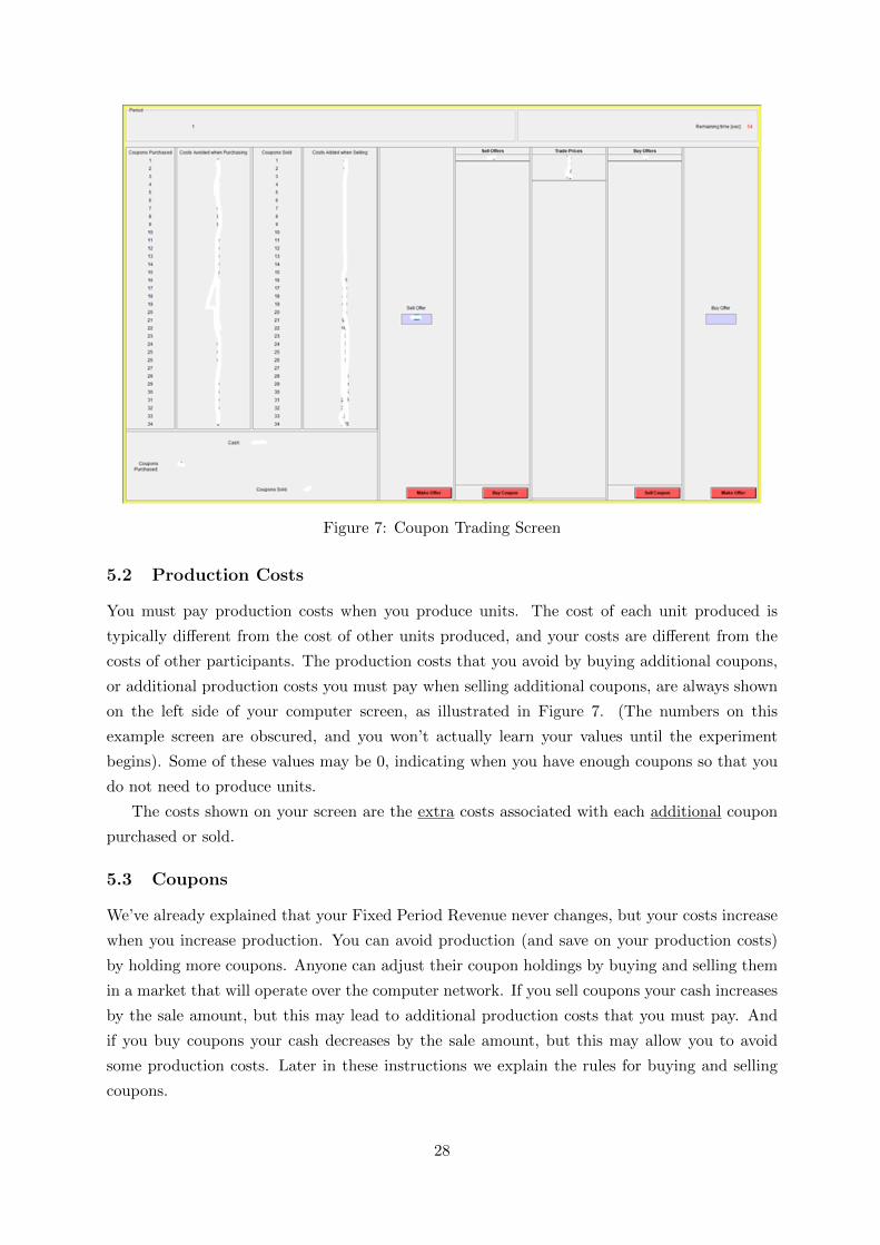
Figure 7: Coupon Trading Screen
5.2 Production Costs
You must pay production costs when you produce units. The cost of each unit produced is
typically different from the cost of other units produced, and your costs are different from the
costs of other participants. The production costs that you avoid by buying additional coupons,
or additional production costs you must pay when selling additional coupons, are always shown
on the left side of your computer screen, as illustrated in Figure 7. (The numbers on this
example screen are obscured, and you won’t actually learn your values until the experiment
begins). Some of these values may be 0, indicating when you have enough coupons so that you
do not need to produce units.
The costs shown on your screen are the extra costs associated with each additional coupon
purchased or sold.
5.3 Coupons
We’ve already explained that your Fixed Period Revenue never changes, but your costs increase
when you increase production. You can avoid production (and save on your production costs)
by holding more coupons. Anyone can adjust their coupon holdings by buying and selling them
in a market that will operate over the computer network. If you sell coupons your cash increases
by the sale amount, but this may lead to additional production costs that you must pay. And
if you buy coupons your cash decreases by the sale amount, but this may allow you to avoid
some production costs. Later in these instructions we explain the rules for buying and selling
coupons.
28
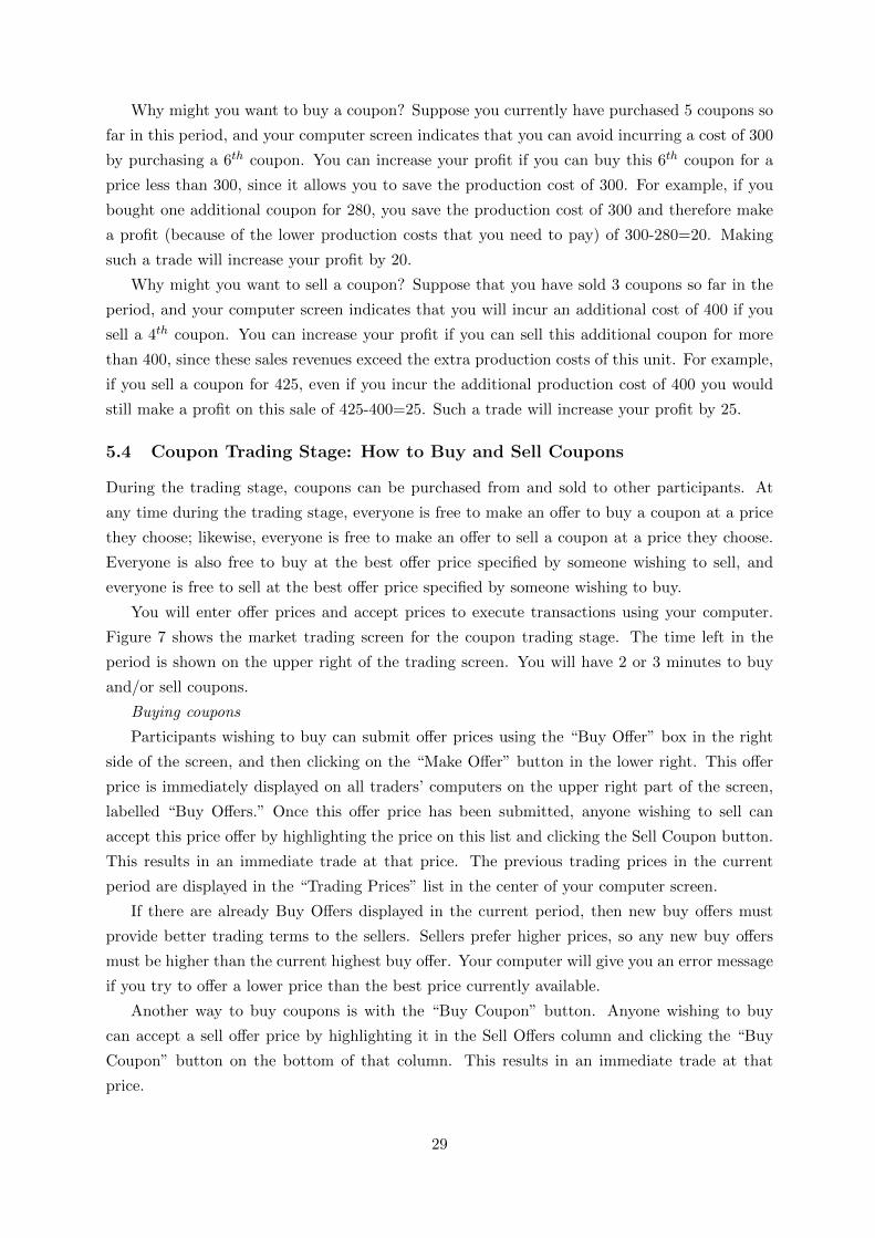
Why might you want to buy a coupon? Suppose you currently have purchased 5 coupons so
far in this period, and your computer screen indicates that you can avoid incurring a cost of 300
by purchasing a 6th coupon. You can increase your profit if you can buy this 6th coupon for a
price less than 300, since it allows you to save the production cost of 300. For example, if you
bought one additional coupon for 280, you save the production cost of 300 and therefore make
a profit (because of the lower production costs that you need to pay) of 300-280=20. Making
such a trade will increase your profit by 20.
Why might you want to sell a coupon? Suppose that you have sold 3 coupons so far in the
period, and your computer screen indicates that you will incur an additional cost of 400 if you
sell a 4th coupon. You can increase your profit if you can sell this additional coupon for more
than 400, since these sales revenues exceed the extra production costs of this unit. For example,
if you sell a coupon for 425, even if you incur the additional production cost of 400 you would
still make a profit on this sale of 425-400=25. Such a trade will increase your profit by 25.
5.4 Coupon Trading Stage: How to Buy and Sell Coupons
During the trading stage, coupons can be purchased from and sold to other participants. At
any time during the trading stage, everyone is free to make an offer to buy a coupon at a price
they choose; likewise, everyone is free to make an offer to sell a coupon at a price they choose.
Everyone is also free to buy at the best offer price specified by someone wishing to sell, and
everyone is free to sell at the best offer price specified by someone wishing to buy.
You will enter offer prices and accept prices to execute transactions using your computer.
Figure 7 shows the market trading screen for the coupon trading stage. The time left in the
period is shown on the upper right of the trading screen. You will have 2 or 3 minutes to buy
and/or sell coupons.
Buying coupons
Participants wishing to buy can submit offer prices using the “Buy Offer” box in the right
side of the screen, and then clicking on the “Make Offer” button in the lower right. This offer
price is immediately displayed on all traders’ computers on the upper right part of the screen,
labelled “Buy Offers.” Once this offer price has been submitted, anyone wishing to sell can
accept this price offer by highlighting the price on this list and clicking the Sell Coupon button.
This results in an immediate trade at that price. The previous trading prices in the current
period are displayed in the “Trading Prices” list in the center of your computer screen.
If there are already Buy Offers displayed in the current period, then new buy offers must
provide better trading terms to the sellers. Sellers prefer higher prices, so any new buy offers
must be higher than the current highest buy offer. Your computer will give you an error message
if you try to offer a lower price than the best price currently available.
Another way to buy coupons is with the “Buy Coupon” button. Anyone wishing to buy
can accept a sell offer price by highlighting it in the Sell Offers column and clicking the “Buy
Coupon” button on the bottom of that column. This results in an immediate trade at that
price.
29

Selling Coupons
Participants wishing to sell can submit offer prices using the “Sell Offer” box in the middle
of the screen, and then clicking on the “Make Offer” button below this box. This offer price is
immediately displayed on all traders’ computers on the upper middle part of the screen, labelled
“Sell Offers.” Once this offer price has been submitted, anyone wishing to buy can accept this
price offer by highlighting the price on this list and clicking the Buy Coupon button.
If there are already Sell Offers displayed in the current period, then new sell offers must
provide better trading terms to the buyers. Buyers prefer lower prices, so any new sell offers
must be lower than the current lowest sell offer.
Another way to sell coupons is with the “Sell Coupon” button. Anyone wishing to sell
can accept a buy offer price by highlighting it in the Buy Offers column and clicking the “Sell
Coupon” button on the bottom of that column. This results in an immediate trade at that
price.
During the experiment, there will be both a minimum and a maximum price for
trading coupons. The minimum is 70 and the maximum is 999. These minimum
and maximum prices will be the same for all periods.
If you submit a bid to buy or offer to sell a coupon that is greater than the
maximum price, then you will receive an error message reminding you of this upper
limit. In the same way, if you submit an offer to buy or sell at below the minimum
price, you will receive an error message.
Regardless of how you buy or sell coupons, your net number of Coupons Purchased or
Coupons Sold, and Cash total, will be updated at the time of purchase or sale. You can always
find these totals in the lower left of the screen.
5.5 Period Structure
This part of the experiment will consist of 16 paid periods, following one unpaid practice period.
Each period is identical and will include the following steps in Figure 8.
5.6 Investment Stage
At the start of each period, you will indicate whether you want to make an investment at a total
fixed cost of 200 Experimental Dollars. If you make this investment, your costs will decrease
from the amounts shown on the left side of your hardcopy coupon trading values sheet (labelled
“Costs with No Investment”) to the amounts shown on the right side of this sheet (labelled
“Costs if Investing”).
5.7 Random Coupons
You and all the other traders today will also receive a random number of additional coupons at
the beginning of the trading stage. There are 5 different possible numbers of coupons you each
might receive, and each of these 5 possibilities is equally likely to occur:
0 Coupons – OR – 1 Coupons – OR – 3 Coupons – OR – 4 Coupons – OR – 5 Coupons
30

6
Figure 2:
Note also: Your coupon trading values shown on your computer screen will adjust to
reflect these random additional coupons, so they will usually not be exactly the same as the
numbers shown on your hardcopy coupon trading values sheet. For example, if you receive 3
additional coupons in the random allocation, this is equivalent to moving you down the list of
costs to 3 purchased coupons. The extra costs avoided by purchasing more coupons, or extra
costs incurred by selling coupons, will be adjusted accordingly. Importantly, you should
therefore consider the costs avoided or added ON YOUR COMPUTER SCREEN rather than on
your hardcopy cost sheet while trading.
Receive Fixed Period Revenue
Investment Stage You will have an opportunity to make an investment, at a fixed cost, which lowers your production cost.
Random Coupons You will receive an additional, random number of coupons
Trading Stage Coupons are traded as explained above.
Computer Sales You can sell additional coupons directly to computer at a price of 69.
Period Results Write down your end of period results on your personal record sheet.
Figure 8: Period Structure
Note: This number of random coupons will typically change from period to period, but the
number is the same for all participants. That is, the number of random coupons you receive is
the same as the number received by each of the other traders in your market.
Note also: Your coupon trading values shown on your computer screen will adjust to reflect
these random additional coupons, so they will usually not be exactly the same as the numbers
shown on your hardcopy coupon trading values sheet. For example, if you receive 3 additional
coupons in the random allocation, this is equivalent to moving you down the list of costs to 3
purchased coupons. The extra costs avoided by purchasing more coupons, or extra costs incurred
by selling coupons, will be adjusted accordingly. Importantly, you should therefore consider the
costs avoided or added ON YOUR COMPUTER SCREEN rather than on your hardcopy cost
sheet while trading.
5.8 Trading Stage
After the investment stage and the random coupons are distributed in the steps described above,
you may choose to buy and/or sell coupons with each other. The trading stage will last 3 minutes
until period 6, when it will shorten to 2 minutes. Remember, you may wish to buy coupons if
the price you pay is less than the production cost that you can avoid; or you may wish to sell
coupons if the price you receive is greater than the additional production cost you must incur.
31

Figure 9: Computer Sales
These amounts are shown on your computer screen.
Importantly, the additional costs incurred or avoided may be different depending on how
many coupons you have bought or sold in the period so far. Therefore, you should always pay
close attention to this information so that you know which unit of coupons you might be buying
or selling next. These total numbers of coupons purchased or sold, as well as your cash totals,
will be updated immediately at the time of purchase or sale on the lower left part of your screen.
5.9 Sales to the Computer
After the market trading stage is completed, you will have a final opportunity to
make sales directly to the central computer, called “Computer Sales.” The software
will consider your costs avoided when selling, and the number of coupons you bought
or sold during the trading period, and as illustrated in Figure 9 it will indicate how
many additional coupons you have with added costs less than 69. The computer
will purchase any of these additional coupons you want to sell at this price. The
number suggested on this screen is the total number of additional coupons you
could sell to increase your earnings in the period if you sell them to the computer.
This number will be 0 if you do not have additional coupons with costs lower than
69.
5.10 Period Results
Once trading has been completed, the results of the period will display on your screen, as
illustrated in Figure 10. You should copy this information onto your Personal Record Sheet,
32
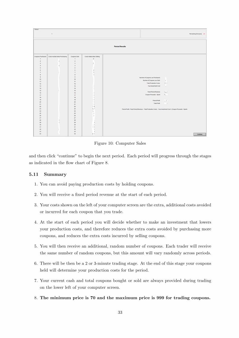
Figure 10: Computer Sales
and then click “continue” to begin the next period. Each period will progress through the stages
as indicated in the flow chart of Figure 8.
5.11 Summary
1. You can avoid paying production costs by holding coupons.
2. You will receive a fixed period revenue at the start of each period.
3. Your costs shown on the left of your computer screen are the extra, additional costs avoided
or incurred for each coupon that you trade.
4. At the start of each period you will decide whether to make an investment that lowers
your production costs, and therefore reduces the extra costs avoided by purchasing more
coupons, and reduces the extra costs incurred by selling coupons.
5. You will then receive an additional, random number of coupons. Each trader will receive
the same number of random coupons, but this amount will vary randomly across periods.
6. There will be then be a 2 or 3-minute trading stage. At the end of this stage your coupons
held will determine your production costs for the period.
7. Your current cash and total coupons bought or sold are always provided during trading
on the lower left of your computer screen.
8. The minimum price is 70 and the maximum price is 999 for trading coupons.
33
9. After market trading is concluded each period, you will have a final opportunity
to sell additional coupons to the central computer at a fixed price of 69.
10. Your coupon sales or purchases, final production costs, and total period profits will be
provided during the Period Results stage at the end of each period. No coupons or cash
will be carried over into the next period for use in trading.
If you have any questions during the experiment, please raise your hand and I will come
to your seat. Are there any questions now before we begin?
34

References
[1] Borenstein, S., J. Bushnell, F.A. Wolak and M. Zaragoza-Watkins (2019), “Expecting
the Unexpected: Emissions Uncertainty and Environmental Market Design,” Ameri-
can Economic Review 109: 3953-3977.
[2] Bos, F., T. van der Pol and G. Romijn (2019), “Should Benefit-Cost Analysis Include
a Correction for the Marginal Excess Burden of Taxation?” Journal of Benefit-Cost
Analysis 10: 379-403.
[3] Brauneis, A., R. Mestel and S. Palan (2013), “Inducing Low-Carbon Investment in
the Electric Power Industry through a Price Floor for Emissions Trading,” Energy
Policy 53: 190-204.
[4] Burtraw, D., K. Palmer and D. Kahn (2010), “A Symmetric Safety Valve,” Energy
Policy 38: 4921-4932.
[5] California Air Resources Board (2021), “Cap-and-Trade Program Recent Market In-
formation,” https://ww3.arb.ca.gov/cc/capandtrade/market_info.htm, Last ac-
cessed January 25, 2021.
[6] Cason, T.N., L. Gangadharan and C. Duke (2003), “Market Power in Tradable Emis-
sion Markets: A Laboratory Testbed for Emission Trading in Port Phillip Bay, Vic-
toria,” Ecological Economics 46: 469-491.
[7] Cason T.N. and L. Raymond (2011), “Framing Effects in an Emissions Trading Exper-
iment with Voluntary Compliance,” In: R.M Isaac and D.A. Norton (eds), Research
in Experimental Economics Vol. 14, Emerald Group Publishing, Bingley, pp. 77-114.
[8] Cason, T.N. and F.P. de Vries (2019), “Dynamic Efficiency in Experimental Emis-
sions Trading Markets with Investment Uncertainty,” Environmental and Resource
Economics 73: 1-31.
[9] Fabra, N., N.H.M. von der Fehr and M.A de Frutos (2011), “Market Design and
Investment Incentives,” The Economic Journal 121: 1340-1360.
[10] Fell H. and R.D. Morgenstern (2010), “Alternative Approaches to Cost Containment
in a Cap-and-Trade System,” Environmental and Resource Economics 47: 275-297.
[11] Fell H., D. Burtraw, R.D. Morgenstern and K.L. Palmer (2012), “Soft and Hard Price
Collars in a Cap-and-Trade System: A Comparative Analysis,” Journal of Environ-
mental Economics and Management 64: 183-198.
[12] Fischbacher, U. (2007), “z-Tree: Zurich Toolbox for Ready-Made Economic Experi-
ments,” Experimental Economics 10: 171-178.
[13] Friesen, L., L. Gangadharan, P. Khezr and I.A. MacKenzie (2019), “Cost Containment
in Pollution Auctions,” Discussion Papers Series 610, School of Economics, University
of Queensland, Australia.
35
[14] Friesen, L., L. Gangadharan, P. Khezr and I.A. MacKenzie (2020), “Mind your Ps and
Qs! An Experiment on Variable Allowance Supply in the US Regional Greenhouse
Gas Initiative,” Discussion Papers Series 618, School of Economics, University of
Queensland, Australia.
[15] Greiner, B. (2015), “Subject Pool Recruitment Procedures: Organizing Experiments
with ORSEE,” Journal of the Economic Science Association 1: 114-125.
[16] Grull, G. and L. Taschini (2011), “Cap-and-Trade Properties under Different Hybrid
Scheme Designs,” Journal of Environmental Economics and Management 61: 107-
118.
[17] Holt, C.A. and W.M. Shobe (2016), “Price and Quantity Collars for Stabilizing Emis-
sion Allowance Prices: Laboratory Experiments on the EU ETS Market Stability
Reserve,” Journal of Environmental Economics and Management 80: 69-86.
[18] Isaac, R.M. and C.R. Plott (1981), “Price Controls and the Behavior of Auction
Markets: An Experimental Investigation,” American Economic Review 71: 448-459.
[19] Jacoby, H.D. and A.D. Ellerman (2004), “The Safety Valve and Climate Policy,”
Energy Policy 32: 481-491.
[20] Johstone, N., I. Hascic and D. Popp (2010), “Renewable Energy Policies and Techno-
logical Innovation: Evidence Based on Patent Counts,” Environmental and Resource
Economics 45: 133-155.
[21] Kotani, K., K. Tanaka and S. Managi (2019), “Which Performs Better under Trader
Settings, Double Auction or Uniform Price Auction?” Experimental Economics 22:
247-267.
[22] Murray, B.C., R.G. Newell and W.A. Pizer (2009), “Balancing Cost and Emissions
Certainty: An Allowance Reserve for Cap-and-Trade,” Review of Environmental Eco-
nomics and Policy 3: 84-103.
[23] Newbery, D.M., D.M. Reiner and R.A. Ritz (2019), “The Political Economy of a
Carbon Price Floor for Power Generation,” The Energy Journal 3: 1-24.
[24] Perkis, D.F., T.N. Cason and W.E. Tyner (2016), “An Experimental Investigation
of Hard and Soft Price Ceilings in Emissions Permit Markets,” Environmental and
Resource Economics 63: 703-718.
[25] Philibert, C. (2009), “Assessing the Value of Price Caps and Floors,” Climate Policy
9: 612-633.
[26] Pizer, W.A. (2002), “Combining Price and Quantity Controls to Mitigate Global
Climate Change,” Journal of Public Economics 85: 409-434.
[27] Requate, T. (2005), “Dynamic Incentives by Environmental Policy Instruments—A
Survey,” Ecological Economics 54: 175-195.
[28] Requate, T. and W. Unold (2003), “Environmental Policy Incentives to Adopt Ad-
vanced Abatement Technology: Will the True Ranking please Stand Up?” European
Economic Review 47: 125-146.
36
[29] Roberts, M.J. and M. Spence (1976), “Effluent Charges and Licenses under Uncer-
tainty,” Journal of Public Economics 5: 193-208.
[30] Salant, S., W. Shobe and N. Uler (2020), “The Effects of ‘Non-Binding’ Price Floors:
Theoretical and Experimental Results,” Working Paper.
[31] Smith, V.L. (1982), “Microeconomic Systems as an Experimental Science,” American
Economic Review 72: 923-955.
[32] Smith, V.L. and A.W. Williams (1981), “On Nonbinding Price Controls in a Com-
petitive Market,” American Economic Review 71: 467-474.
[33] Stranlund, J.K. and L.J. Moffitt (2014), “Enforcement and Price Controls in Emis-
sions Trading,” Journal of Environmental Economics and Management 67: 20-38.
[34] Stranlund, J.K., J.J. Murphy and J.M. Spraggon (2014), “Price Controls and Bank-
ing in Emissions Trading: An Experimental Evaluation,” Journal of Environmental
Economics and Management 68: 71-86.
[35] Stranlund, J.K. and I. Son (2019), “Prices versus Quantities versus Hybrids in the
Presence of Co-pollutants,” Environmental and Resource Economics 73: 353-384.
[36] Tanaka, T., M. Sekito, S. Managi, S. Kaneko and V. Rai (2017), “Decision-Making
Governance for Purchases of Solar Photovoltaic Systems in Japan,” Energy Policy
111: 75-84.
[37] Taylor, M.R. (2012), “Innovation under Cap-and-Trade Programs,” Proceedings of
the National Academy of Sciences 109: 4804-4809.
[38] US Congressional Research Service (2019), “The Regional Greenhouse Gas Initia-
tive: Background, Impacts, and Selected Issues (R41836),” Available at https:
//crsreports.congress.gov/, Last accessed January 25, 2021.
[39] Weber, T.A. and K. Neuhoff (2010), “Carbon Markets and Technological Innovation,”
Journal of Environmental Economics and Management 60: 115-132.
[40] Weitzman, M.L. (1974), “Prices vs. Quantities,” Review of Economic Studies 41:
477-491.
[41] Wood, P.J. and F. Jotzo (2011), “Price Floors for Emissions Trading,” Energy Policy
39: 1746-1775.
[42] Zhao, J. (2003), “Irreversible Abatement Investment under Cost Uncertainties: Trad-
able Emission Permits and Emissions Charges,” Journal of Public Economics 87:
2765-2789.
37