Investment in Public Infrastructure and Tax

Competition between Contiguous Regions

Carole Dembour∗and Xavier Wauthy†

October 16, 2003

Abstract

Two contiguous regions compete to attract a population of het-erogeneous firms. They choose infrastructure levels in a first stage,then compete in tax. We compare the properties of subgame perfectnash equilibria in this stage-game depending on the intrisic featuresof the infrastructure considered. Then we derive some implicationsregarding the scope for cooperation between the regions.

1 Introduction

The last decades have been marked by a sharp decrease of transportationcosts, and more generally trade costs, together with an increased mobilityfor capital and to a lesser extent of the labour force caused by institutionalfactors. As a result, the location of firm’s productive activities is more andmore disconnected from the destination market of their final products. Be-cause firms are more mobile, national or regional governments have becomemore and more concerned by tax competition issues. In particular, by therisk that firms actually bid up local authorities one against the other to ob-tain tax reliefs. Observations suggests that the risk is indeed present. Forinstanc eSorensen (2000) presents evidence of a significant fall in capitalnominal tax rate from the 80’s to the end of the 90’s.

A growing body of the literature deals with tax competition games.Fortunately this literature most often conclude to the development of amitigated tax competition. In a sense, tax revenues may not decrease thatmuch because of tax competition. At the same time, it is obvious the

∗CEREC, FUSL. The research of Carole Dembour benefited from the financial supportof the Region de Bruxelles-Capitale ’s government under the Prospective Research forBrussels program.

†CEREC, FUSL and CORE, UCL

1

fiscal motives are not the only reason why firms would delocalize produc-tion. The specific amenities of regions, be it exogenous or resulting fromagglomeration externalities, enter the picture as well. Public authoritiesare not passive either in this respect. In particular they tend to attractfirms by magnifying their local amenities, and/or stimulating the emer-gence of strong spatial externalities. Thus, local authorities may affectfirms’ location decisions in essentially two ways: by offering an attractivefiscal package, and by developing a favorable economic environment (en-hancing the quality of their infrastructure, braodly defined). Head and al.(1999) conducted an empirical analysis revealing how sensitive firms canbe to non-fiscal arguments.1As argued recently by Justman et al. (2003) itmay actually be the case that by specializing their infrastructure packages,regions may in fact relax tax competition.2

In the literature dealing with regional competition, When local author-ities compete one against the other at the level of taxes as well as at thelevel of infrastructure, it is most often assumed that the infrastructure of-fer is specific to each region. Justman and al. (2001) is a good example.Therefore, regional infrastructures are viewed as substitutes from the pointof view of the firms. This is clearly reasonable when regions really differ ingeographical locations, i.e. they are located at a significant distance fromeach other. Suppose by contrast that a well-defined economic activity areais actually divided in two (or several) political regions, each endowed withsome fiscal autonomy.3. In a sense firms actuallly contemplate the possi-bility of locating their activities in the economic area, as a whole. Then, ifthey chose to move to the area, they would have to address the question ofwhere (i.e. in which political region) to locate within the area. The choiceof a particular region will reflect the presence of tax differentials ans well aspossible differences in the in frastructure supplied by the regions. However,if regions are contiguous, it might difficult to argue that the benefits ofan infrastructure developed by one of the regional government is entirelyconfined to its political frontiers. In many cases, a ”local” infrastructurewill inevitably see its ”benefits” spillover accross political entities to thewhole economic bassin. If this is the case, then an infrastructure located inone region might be viewed as a complement to the development strategyof the other entities. Think for instance of an airport terminal located inone region. Clearly enough, this infrastructure increases the attractivenessof the region. However, it is hard to see why it would not increase that

1See also Dembour (2003) for a recent selective survey on theoretical models dealingwith competition for business units.

2More generally, local authorities are very likely to transfer tax competition towardsless direct fields. See Peralta and al. (2003).

3As is typically the case for the region of Bruxelles Capitale in Belgium

2

of the contiguous regions as well. Most reasonably, this infrastructure in-creases the attractiveness of the economic area as a whole. By contrast,the positive impact of a high speed telecommunication network could bemore easily restricted to one region region only. Similarly, it is reasonablyeasy to condition access to ”administrative” support services on the fiscallocation of firms.

The present note builds on this intuition. We consider a model whereregions compete for firms by choose the ”quality” of the infrastructure theywill offer to the firms. They also compete in taxes. Regarding infrastruc-ture, the critical issue is the extent to which the infrastructure proposed byone the region is truly specific to this region or spills over to the contiguousones. We shall consider the two polar cases of a strictly regional-specificinfrastructure and an infrastructure whose effects are equally distributedaccross regions. In the first case, infrastructure is a pure private goodwhereas in the second case, it is a pure public good.

We address two questions: to which extent does the economic natureof the infrastructure alter the equilibrium behaviour of regions? To whichextent does the nature of the infrastructure enhances or hinders cooperationbetween regions?

Part of the regions’ problem can then viewed as follows: regions couldfind interesting to cooperate at the level of infrastructure, and the moreso the more they are closely connected, while being competitors at thefiscal level. Cooperation at the infrastructure level seems desirable if bothregions benefit from the increased attractiveness of the area. However, sinceinfrastructure as the attribute of a public good, each region is likely to adopta free rider behavior, thereby inducing too low a level of investment.

In order to address these questions, we build a stylized model inspiredby the canonical location model of Hotelling (1929). This model will allowto formalize regional competition as a two-stage between two contuguous,though different, regions. In a first stage regions choose infrastrucutre levelsnon-cooperatively, in a second stage they set taxes non-cooperatively. Thenfirms decide on locations. Our equilibrium concept is subgame perfect Nashequilibrium. Our analysis also rests on a 2 by 2 typology characterizing theinfrastructure’s type. On the one hand, infrastructure benefits may eitherbe strictly localized or strictly non-localized. On the other hand the benefitsmight be either depedent or independent on firms’ types. We show that thescope for regional cooperation is highly dependent on the characteristics ofthe infrastructure, because these characteristics impact differently the taxcompetition stage.

In the next section, we present the basic model. Section 3 is devotedto the analysis of infrastructures that affect firms symmetrically. We char-

3

acterize subgame perfect equilibria.4 Then, in section 4 we draw someimplications of our findings and discuss extensions of the basic model.

2 A Model

Let us denote by C a well-defined economic area (for simplicity we shalltalk of the ”country”, when referring to the economic area C) which isdivided in two contiguous ”regions” (in the following, ”regions” designatelocal political entities): A and B.

2.1 The Firms

There is a continuum of heterogeneous mobile firms contemplating to re-locate their activities in C. Each firm is identified by a type x. Typesare uniformly distributed in the continuous [0, 1] interval. The density isnormalized to 1 so that the total number of firms is also n,ormalized to 1.These firms are supposed to be located somewhere outside C and if theydecide not to move to C, they enjoy a reservation profit π. Thus, π definestheir status quo option.

Firms’ types can be understood as designating some technological speci-ficities of the firm that will have to be matched to in area C. These typesare for instance related to the particular industry in which the firm is ac-tive. It could consist of a specific know-how that has to be taugth to newworkers. The matching cost contributes to define the fixed cost the firmwill have to bear if it chooses to locate in area C. Obviously, this cost mayalso depend on the region in which it chooses to locate. Indeed, regionsthemselves display a priori characteristics inherited from their own history.The key point at this step is to assume that regions and firms are heteroge-neous. To capture this idea, we assume that each region is located at onepoint xA, xB respectively. For simplicity, we assume xA = 0, xB = 1.

The matching cost of a firm with type x ∈ [0, 1] depends positivelyon the ”distance” from the region’s location.5 We may therefore define amatching cost function for each region: mA(x), mB(1 − x). Finally, wedenote by tA and tB the lump-sum fee each region levies on firms.

Under the preceding assumption, we formalize a firm’s location decisionas follows: a firm chooses the location where its profit is larger. Thisprofit is defined as the operating profit (i.e. the profit resulting from the

4The parallel analysis for type dependent benefits of infrastructure is developed in theAppendix.

5note that the term location should not be understood here in the geographical sense.Firms are located in the characteristics’ space.

4

production activity)6 minus the matching cost and the lump-sum tax. Incase the firm does not move to country C (stays abroad), the ”status quo”profit is defined by π. Moving to area A yields a payoff:

πA(x) = KA −mA(x)− tA, (1)

whereas moving to region B yields:

πB(x) = KB −mB(1− x)− tB, (2)

where Ki denotes operating profits in region i.

2.2 The Regions

Regional authorities choose the infrastructure they supply to the firms.They also choose tax levels non-cooperatively. Given the specification offirms’ profits as a function of location (equations (1) and (2)), two typesof infrastructure can be distinguished: either it affects the matching cost(negatively) or the operating profits (positively). In both cases, the attrac-tivness of the region is reinforced if the quality of infrastructure supplied tothe firms is increased. Infrastructure levels are committed to by the regionsin a first stage, than tax levels are set simultaneously in a second stage.

Two basic type of infrastructures must be distinguished because theyhave different implications in a world where tax competition takes place.We may consider first infrastructures whose benefits to a firm depends onthe type of this firm. This is especially true of a training program aimedat matching local workers’ qualifications to incoming firms’ needs, or of adevelopment office aimed at helping firms to install their administrativeand sales network. On the other hand, infrastructures such as the supplyof public transport or high speed communication networks benefit havetheir benefits more uniformly distributed accross firms. Moreover, they arerecurrent benefits related to the daily activity of incoming firms whereasthe previous examples were related to the installation costs of the incomingfirm. We shall show later on that these two infrastructure types havedifferent implications on the tax competition game.

A last feature of infrastructure expenses must be considered: the lo-calization of its effects. Two polar cases are considered hereafter. Eitherthe infrastructure is entirely general. This implies that any firm locating

6For instance, Justman et al. (2000) assume the following operating profits structure:Firms produce according to a production function y(l) = lα, where l designates units oflabor input and 0 < α < 1. Labor is homogeneous perfectly mobile within C so that thewage prevailing in the two regions is identical and given by w. Operating profits are thusdefined as y(l)− wl.

5

in country C benefits from the infrastructure symmetrically. In this case,any infrastructure investment by one region increases the attractiveness ofthe whole area, without giving any specific advantage to this region. Atthe other extreme, we shall consider the case of a purely specific7 infras-tructure with i = A,B. In this case, the infrastructure benefits to a firmonly if the firm locates in the specific region where the infrastructure hasbeen installed. Accordingly, no region can benefit from the infrastructureinstalled by the other one. In this context, providing more infrastructurein the first stage is apt to give a competitive advantage in the second stage:being more attractive, the high infrastructure region can attract firms evenif taxes are significantly higher than in the contiguous region.

The objective of the local authorities is to maximize regional Welfare,defined as the wage bill in the region minus the cost of infrastructure plusthe tax revenue (or minus the subsidy expenses).

Wi = w ∗ Li + tiMi − c(Ki)

where Li denotes the labour demand of the firms located in the region, Mitiis the tax revenue and c(Ki) is the cost of infrastructure. For simplicity, weassume ti ≥ 0, i.e. regions are not allowed to offer net subsidies to firms.We do not impose in this paper any explicit budget constraints. Obviously,this does not mean that the cost of public fund is zero in the model. Indeedlower taxes and infrastructure expenses affect the objective negatively.8

2.3 The Game

We solve the following stage game

• Stage 1: Regions decide simultaneously on infrastructure levels.

• Stage 2: Regions decide on tax levels with infrastructure levels beingpublicly observed, choosing ti ≥ 0

• Stage 3: Observing infrastructure decisions and taxes, firms decide oftheir location

7The specificvs general typology is inherited from Labour economics, where humancapital is said to be ”general” if transferable from one firm to another.

8In section 4, we nevertheless discuss the implications of specific budgetary constraintsthat could apply to local authorities. It is indeed often the case that regional author-ities face constitutional constraints which limit their ability to display budget deficits.Obviously, this is likely to affect equilibrium behaviour.

6

3 Infrastructure with Uniform Benefits

In this section, we assume that decisions made regarding infrastructurealter the operating profits of firms, i.e. the term Ki in equations (1) and(2).9 Note that a key feature of this type of infrastructure is that it affectsequally all the firms that choose to locate within a given region.

3.1 The Public Good Case

In the pure public good case, any invesment by one of the region affectsKi symmetrically. We shall assume for simplicity that in (1) and (2), wehave KA = KB = K, where K depends positively and symmetrically of theinvestments realized by either regions. Thus, the level of K will be used asa proxy for the quality of the infrastructure supplied by the regions.

•We first characterize firms’ equilibrium behaviour at stage 3, i.e. firms’optimal choices given K and ti.

Given its outside option π, each firm compares π, πA(x) and πB(x).Two types of configurations must be distinguished:

• (K, ti) are such that some firms are better off choosing their outsideoption. We shall denote such configurations as non-covered ones

• (K, ti) are such that all firms are attracted in country C. Theseconfigurations will be referred to as covered configurations.

For a non-covered configuration to prevail, there must exist some type x

such that max{πA(x), πB(x)

}< π. Focusing on the possibility of locating

in, say, region A, or not moving at all, any firm x compares K−ma(x)− tAto π. Solving

K −ma(x)− tA = π

for x, we identify the subset of firms preferring to move to region A ratherthan enjoying the status quo. Let us denote this set of firms by MA.

Performing a similar analysis for region B allows us to define a anotherset MB which contains those firms willing to move to region B if the al-ternative is the status quo. Obviously, non-covered configurations prevailwhenever require that [0, 1]/(MA ∪MB) defines a non empty set.

In order to obtain closed form solutions, we shall assume from now that

ma(x) = mx and mb(x) = m(1− x) with m > 0 (A1)9Think for instance of an investment increasing labour productivity, or a .

7

Moreover, we assume without loss of generality that π = 0.10

Using (A.1), the fact that the distribution is uniform in [0, 1] and thedensity is 1, we compute the number of firms locating in both regions. Wesolve K −mx− tA = 0 and K −m(1− x)− tB = 0 to obtain11

MnA =

K − tAm

(3)

MnB = 1− K − tB

m. (4)

Notice that MnA > 1 whenever K − tA > m (resp. Mn

B < 0 wheneverK − tB > m). This condition therefore identifies the constellations whereall firms prefer region A (resp. B) to the status quo.

Direct computations using the above expressions indicate that MnA <

MnB whenever 2K−m > t. When 2K−m < t, no firm prefers the status quo

to locating in at least one region, i.e. we have a covered configuration. Forsuch configurations it then remains to characterize in which of the regionsA or B will a firm with type x locate. To answer this question we solveK −mx− tA = K −m(1− x)− tB to obtain:

x̃(tA, tB,K) =m− tA + tB

2m(5)

Any firm with type x < x̃ locates in region A whereas firms with typesx >: tildex locate in region B. We have12

M cA =

m− tA + tB2m

(6)

M cB = 1− m− tA + tB

2m. (7)

It then remains to check for the boundary conditions, i.e. the con-ditions which ensure that the number of firms locating in each region isnon-negative. Using equation (6) and (7) we obtain:

0 < x̃ < 1 ⇐⇒ −m < tA − tB < m

.

Proposition 1. The equilibrium partition of the firms in stage 3 is definedas follows:

10Notice that under (A1), our model is formally equivalent to the generic Hotellingmodel with linear transportation costsd and endogenous market coverage.

11The upperscript n denotes the non-covered configuration.12The upperscript c denotes covered configurations.

8

• Whenever 2K−m ≥ tA+tB a non-covered configuration prevails. The

number of firms locating in region A is given by max{0,min

{1,Mn

A

}}.

The number of firms locating in region B is given by max{0,min

{1,Mn

B

}}.

• Whenever 2K −m < tA + tB, a covered configuration prevails. The

number of firms locating in region A is given by max{0,min

{1,M c

A

}}.

The number of firms locating in region B is given by max{0,min

{1,M c

B

}}.

Figure 1 illustrates Proposition 1 by partitioning the (tA, tB) space ac-cording to the firms’ optimal choices.

Insert figure 1 about here

We may restrict attention to the sub-domain where ti ≤ K. Indeed,ti > K is clearly a dominated strategy. There are then 4 areas of interest.In Area I, each region benefits from a local monopoly: regions are notcompetition among themselves but each are separately competing with thestatus quo option. In Area IIA, they are truly competing with each other.In Area IIC and IIB, tax differentials are so large that only one regionattracts all the firms.

• We are now equipped to solve for the second stage of the game whereregions compete in taxes.

In order to simplify the exposition, let us first neglect the wage billcomponent of the Regions’ objective function13 so that we are left, in stage2, with two regions wishing to maximize tax revenues.14.

Figure 1 provides a useful benchmark to understand the nature of taxcompetition in this game. In Area I, region’s payoffs are independent. Wemay then characterize a region’s optimal behaviour by maximizing tAMn

A

over tA. We obtain

tnA = tnB =K

2(8)

The corresponding partition of firms is given by MnA = K

2m and MnB =

1 − K2m . This solution is feasible if only we are indeed located in Area I.

Solving 2K −m < tnA + tnB we obtain the necessary and sufficient condition

K < m. (C1)13We discuss the implication of this assumption in the last section of the paper.14Recall that since we do not consider for the moment any explicit budget constraint,

infrastructure expenses made in stage 1 are totally irrelevant in stage 2, i.e. they arepure sunk costs.

9

Turning to Area II we note that there cannot be an equilibrium in areaIIB or IIC. Indeed, in these areas, one region enjoys a zero payoff since nofirm locates in the region15 On the other hand, it is always possible for thisfirm to name a lower tax, that leads to Area IIA where its payoff is positive.Accordingly, we concentrate on the payoffs in Area IIA. Observe that thesepayoffs are now interdependent through the definition of x̃(tA, tB). We solvefor a Nash equilibrium. Maximizing tiM

ci over ti, we obtain the following

specification for regions’ best reply functions:

ϕi(tj) =m + tj

2(9)

Straightforward computations lead to the following characterization of Nashequilibrium taxes:

tcA = tcB = m (10)

All firms on the left of type x = 12 locate in region A whereas the com-

plement locates in region B. It then remains to verify that this solution isindeed defined in Area IIA. To this end we check that 2K −m > tcA + tcB.We obtain the necessary and sufficient condition

K ≥ 3m

2. (C2)

Combining C1 (the feasibility condition for the non-covered interiorequilibrium with that of the interior covered equilibrium (C2), we observethat none of them is satisfied in the sub-domain k ∈ [m, 3m

2 ]. In such cases,a continuum of corner solutions exists. It is defined by:

tcorb ∈ [min

{K

2,4K

3−m

}, 2K −m− t−A] (11)

with t−A = min{

K2 , 4K

3 − m}. We do not develop the characterization of

these corner solutions. The intutition underlying their existence is bestsummarized referring to figure 2.

Inser Figure 2 about here

For intermediate values of K relative to m, each region’s best replyconsiste of three segments: first there is the segment ϕi, up to the frontierbetween Area I and II. Then there is the frontier itself, down to tni thentni . Corner solutions are thus located along the frontier.

We may now summarize the characterization of equilibrium tax ratesas a function of the values of K, that result from first stage choices.

15One could think here of a variant of the modelwhere the payoffs in these areas mightbe positive, and increasing in the number of firms located in the other region. Thiscould be the case with a spillover effect. Typicallly, attracting firms might require a taxdecreases which may not compensate for the gain.

10

Proposition 2a. Nash equilibrium tax rates in stage 2 are given by:

• tcA = tcB = m whenever K ≥ 3m2

• (tcorA , tcor

B ) whenever K ∈ [m, 3m2 ]

• tnA = tnB = K2 whenever K ≤ m.

• Using the above proposition, we analyze now the first stage of thegame where region choose infrastructure levels.

In order to capture the idea that the regions’ respective infrastructureare public goods, we simply assume that the aggregate level K is defined bythe addition of regional infrastructure levels. Stated differently, we assumeK = KA + KB. In the first stage of the game, regions are assumed tochoose (KA,KB) simultaneously and non-cooperatively.

Insert Figure 3 about here

Figure 3 partitions the strategy space according to the nature of taxequilibrium that will follow the corresponding infrastructure choices. Thereare obviously three areas of interests. A key feature of Area a is that regions’payoffs in the tax game do not depend on infrastructure levels. Accordingly,even when infrastructures are almost not costly , no (KA,KB) pair in theinterior of Area a can be part of a subgame perfect equilibrium. In Areab, the corner solution prevails. It is again easy to show that no subgameperfect equilibrium can exist in this Area.16.

The following Proposition summarizes the previous finding.

Proposition 3. When the infrastructure is a public good, there exists noSPE involving KA + KB > m.

We are thus left with candidates SPE in the interior or at the frontierof Area c. Suppose that infrastructure costs are zero, then we cannot havean equilibrium in the interior of Area c. Since only the aggregate levelmatters, each region is willing to complement the other’s investment upto Ki = m − Kj . Accordingly, we expect to end up with a continuumof subgame perfect equilibria characterized by K∗

A + K∗B = m whenever

infrastructure costs are low enough. Notice that the marginal value ofinvesting in infrastructure is constant and in particular does not depend onthe possible difference KA−KB. Accordingly, regarding investment levels,each region is actually willing to invest up to the level of infrastructure itwould invest for itself, should it be alone.

16Notice that we face here an additional problem: the existence of mutliple equilibria

11

In Area c region A’s payoff in stage 2 is given by K2

4m . The marginalbenefit of increasing K is therefore given by K

2m . Denoting the cost ofinvesting up to an infrastructure level Ki by C(Ki), the optimal level ofinfrastructure in the aggregate is the level for which K

2m = ∂c∂K . Let us

denote this level by K∗ < m. Then, we may claim that against any KB <K∗ region A will complement region B’s investment in order to ensure thatKA + KB = m as long as KA < k∗. It follows that equilibrium in the firststage can be summarized as follows:

Proposition 4. When infrastructure is a pure public good, there existsa continuum of SPE with the following features: any pair (KA,KB) suchthat KA + KB = m and Ki ≤ K∗ for i = A,B is part of an equilibrium.In the ensuing subgame, regions announce the equilibrium taxes tnA = tnB.All the firms are attracted in country C and each region hosts half of thefirms.

This Proposition may seem surprising. Indeed, it essentially states thatin a SPE, i.e. when regions behave non-cooperatively, they jointly investso as to acheive the efficient level of infrastructure. This is especiallly sur-prising if one recalls that the infrastrcuture is a public good. In such casesindeed, it is traditionally accepted that under-investment should prevailina Nash equilibrium. Should we conclude that in the present framework,players manage to get rid of the free-riding problem that occurs when con-tributing to a public good? The answer is no. The problem regions face herecan be summarized as follows: If they choose infrastructure simultaneously,the realization is likely to be ”too much” or ”too few” investment, which inboth cases are problematic. Either because too few firms are attracted inthe region or because too much money is spent on attracting them. How-ever, from a individual viewpoint, the marginal value of complementing theother’s investment is only related to the number of firms that will end upin the specific region. Thus given that the other has invested too little, i.e.some firm would not be attracted, it is a best response to contribute up tothe required joint level. Actually the free-riding issue is at work. Indeed, inorder to avoid inefficient realization of the equilibrium, regions could playin sequence. But then a very clear first mover advantage appears. If it canindeed commit not to revise his decision, the first mover will invest onlym−K∗ because it is then a best reply for the follower to contribute for theremaining. Thus, free-riding will take the form of competing for leadership.If they both act as leaders, only 2(m−K∗) is invested.

12

3.2 The Private Good Case

The previous analysis has been performed under the assumption that in-frastructures developed in some region was equally beneficial to any firmlocating in the country. In other words, the benefits of the infrastructurespilled over throughout the whole country. We now turn to the case wherethese regional investments benefit to the firms if and only if they locatewithin the region. In other words, access to the infrastrcture can be deniedon a location basis. Infrastructure can then be viewed as a local privategood: a firm ”buys” the good by locating in the corresponding region. Inthis context, investing in infrastructure increases the attractivness of coun-try C only to the extent that firms are willing to locate in the region thatinitiates the investment.

We shall not develop the analysis of the three stage game in full details.Indeed, the formal derivation is similar to that developed in the previoussubsection. Rather, we focus on the key differences that emerge in the gamewhen we switch from the public good infrastructure to a private good one.

The key difference between the two approaches is simple to understand:because they are exclusive attributes of each region, infrastructure levelsnow affect the relative attractivness of a region (i.e. in comparison to thecontiguous one) in addition to its absolute attractivness (which refers thecomparison with the status quo).

Firms now compare KA−mx− tA, KB −m(1− x)− tB and the statusquo (which we normalize again to zero). Focusing on the last stage of thegame, we may adapt Figure 1 to depict the possible distribution of thefirms on the (tA, tB) space. This is done in Figure 4.

Insert Figure 4 about here

With respect to non-covered configurations the structure is essentiallyidentical to the previous case. However the equation of the frontier betweenAre I and II is now given by KA +KB−m = tA + tB. Obviously, differentinfrastructure levels induce an asymmetry between regions that will resultin asymmetric market coverage.

The formal specifications of firms’ distribution accross regions is Mni =

Ki−tim with i = A,B for non-covered configuration. For covered configura-

tions, we may identify the firm which is indifferent between the two regions.The type of this firm, which we denote by x̃(.) is now equal to

x̃(tA, tB) =m + KA −KB − (tA − tB)

2m. (12)

The above equation indicates that when infrastructure are private goods,they will matter in the covered configurations only to the extent that they

13

exhibit different levels.17 This is also materialized by the fact that thefrontiers separating areas IIB and IIc from IIa may not be symmetricallypositioned.18

We may then turn to the analysis of the tax competition game. Optimalbehaviour in non-covered configurations is now directly related to eachregions’ investment levels:

tnA =KA

2with corresponding Mn

A =KA

2m. (13)

As for covered configurations direct computations yield the following bestreply function:

χi =tj + m + Ki −Kj

2. (14)

This expression has to be compared with ϕ in the public good case (seeequation (5)). The comparison illustrates the key difference between thetwo models: when infrastructure are purely private goods, investing morethan the other has a strategic value in the tax competition game. Takingthis into account we may characterize Nash equilibrium in the tax gamefor covered configuration. Last, checking the interiority conditions for theabove candidate equilibria in their respective domainss we identify againa domain for (KA,KB) values where the equilibrium consists of a cornersolution, which we denote tcor

i . Summing up we obtain the following propo-sition, which parallels proposition 2a for the private good case

Proposition 2b. In the private good case, the Nash equilibrium tax ratesin stage 2 is given by:

• tci = m + ki−kj

3 with x̃ = 12 + KA−KB

6m whenever KA + KB ≥ 3m

• (tcorA , tcor

B ) whenever KA + KB ∈ [2m, 3m]

• tni = Ki2 whenever K ≤ 2m.

Relying on the above proposition, we go backward in the game tree andanalyze the first stage. There are three configurations of interest in the(KA,KB) space. Either both infrastrcuture levels are small and the un-covered configuration prevails, or we have a domain of intermediate valueswhere the ensuing tax game exhibits corner equilibria. Last, for high levelsof Ki, a covered configuration prevails in the ensuing tax game. In orderto study optimal infrastructure choices in each case we assume

C(Ki) =K2

I

F, (A2)

17This expression is best understood when compared to equation (5) which applied inthe public good case.

18The frontier between IIa and IIb is for instance given by tA = tB + m + KA −KB

14

with F > 0.Figure5 depicts the relevant somains in the (KA,KB) space.

insert Figure 5 about here

Under non-covered configurations, regions’ equilibrium welfare in stage2 is equal to K2

A4m − K2

AF . This expression is strictly increasing and convex

in the domain where KA > 0 whenever F > 4m. In this case, a region’soptimal investment decision is to maximize Ki. Otherwise the ptimal in-vestment is zero. Therefore, whenever F > 4m, the best reply of region ito any Kj < 2m is Ki = 2m−K − j.

When a corner solution prevails in the tax game, i.e. in the domainwhere KA + KB ∈ [2m, 3m], there is a continuum of tax equilibria. Inany of these equilibria, at least one region obtains a payoff which is strictlyincreasing in Ki whenever F > 4m. Therefore, this region is better off devi-ating upwards, to the boundary KA +KB = 3m. Proposition 5 summarizesour analysis of the two first configurations.

Proposition 5. Suppose investment cost is defined by (A2). Then, inthe private good case, there exist no subgame perfect equilibrium in thenon-covered domain, nor in the interior of the corner solution domain.

Notice that this proposition can be viewed as the exact opposite toProposition 3: indeed, it implies that, contrarily to the public good case, asubgame perfect equilibrium must belong to the sub-domain where coveredconfigurations prevail in the tax subgames.

Contrarily to the case of a public infrastructure, each region’s payoffs aredependent on both KA and KB in covered configurations. More precisely, aregion’s equilibrium gross welfare, i.e. neglecting investment costs, is givenby:

(m +Ki −Kj

3)(

12

+Ki −Kj

6m) (15)

This expression is clearly convex in Ki and reaches a minimum forKi = 3m −Kj , i.e. precisely along the lower bound of the domain wherecovered configurations prevail. Accordingly, as far as tax revenues are con-cerned, regions are always willing to increase Ki in the covered configurationdomain. The upper limit to investments should come from costs. Usingequation (15), we express a region’s net welfare as:

W ∗i (Ki,Kj) = (m +

Ki −Kj

3)(

12

+Ki −Kj

6m)− K2

i

F(16)

15

This expression is globally concave whenever F < 18m19. In this domain,region i’s best reply in the first stage is given by:

Ki(Kj) = (3m−Kj)F

18m− F(17)

Straigthforward algebra yields the subgame perfect equilibrium candidate:

K∗A = K∗

B =F

6. (18)

It then remains to check for interiority conditions, i.e. K∗A + K∗

B ≥ 3m.This condition is satisfied whenever F ≥ 9m. We have thus establish thefollowing proposition:

Proposition 6. Suppose costs is defined by (A2) and infrastructure areprivate goods. Then, whenever F ∈ [9m, 18,m], there exists a uniquesymmetric subgame perfect equilibrium. In this equilibrium, regions investin infrastructure up to K∗

A = K∗B = F

6 ; equilibrium taxes are t∗A = t∗B = mand each region hosts half of the firms.

Proposition 6 Should be contrasted with Proposition 4. It show sin-deed that for a non-trivial domain of the parameters, where investmentscosts take intermediate levels, the non-cooperative behaviour of the regioninduces too much investments. Indeed, part the amount invested is stricltyunvaluable to the regions (although it increases firms’s rent).

4 Comments and Extensions

In this section, we discuss some obvious limitations of the present model aswell as possible extensions. Last, we identify the scope for regional coop-eration as it is revealed by the outcome of the non-cooperative behaviourof the regional governments.

4.1 Budget Constraints

The analysis has been performed without any explcit budget constraint. Asalready mentioned, we assumed that public funds were costly since expensesor lost taxes affect a region’s welfare negatively. However, in reality, local orlocal public authorities may face binding constraint, for instance becausethe constitution does not allow for too large a deficit, or imposes strictbudget balances. A possibly important implication of such constitutionalaspects is that regions may actually be heterogeneous with respect to fiscalissues.

19Should F ≥ 18m the function would be convex and the game has no solution.

16

One easy way to introduce such an asymmetry in the model is to putsome explicit weight λi in the objective function of each region, in orderto reflect the fact that the cost of public funds differ, depending on eachregion’s fiscal global balance. As long as the λi is assumed to be constant,our results will not be qualitatively affected. However, assuming that λi

depends on the budget balance as it results from the model (i.e. λi is afunction of Ki and ti) severely complicate the picture. The following limitcase may provide some intuition about the nature of the problem at stakehere.

Suppose that infrastructure investments must be financed ”within themodel”, i.e. we assume that at the beginning of the game, regions arealready budget constrained while the constitution imposes strict budgetbalance. Thus, any investment aimed at attracting firms must be financedby the tax levied on the incoming firms. This obviously affects the rule ofthe game since any investment committed to in period 1 fixes a lower boundon the minimum tax revenue a region must secure in stage 2. Moreover,tax revenues of a region depends on the tax pair (tA, tB), and not only onthis region’s actions. We plan to pursue the analysis of such situations infuture research.

4.2 Reducing Firms’ Matching Costs

Up to now we have considered the case where regional infrastructure aimedat decreasing sunk costs uniformly accross firms. However, it seems reason-able to assume that depending on their specific type, firms value regionalpolicies differently. This is for instance the case of training programs aimedat matching workers’ qualifications to the firms requirements. The actualvalue of such a program is typically dependent on the firms’ types. To whatextent do the implications of such policies differ from those emphasized inthe case of Ki infrastructure?

In our model, such policies can be captured by assuming that theydecrease m. A region is more likely to host some given firm if it commitsto take part of its matching cost in charge. Formally, we alter our basicmodel as follows:

• First we define matching costs mA(x) = 1−xqA

and mBx = 1−xqB

• In the public good case, we assume qA = qB = qC whereas for theprivate good case, each region is characterized by its specific qi

• Then we solve the model using the same methodology than in theprevious section.

17

The analytical developments have been relegated to the appendix. Theanalysis reveals contrarily to the case where investments affect Ki, the factthat infrastructure are private goods is not sufficient to remove the multi-plicity of subgame perfect equilibria. Actually, when investments are aimedat decreasing mi regions always end up on the frontier which separates non-covered configurations from covered ones. The intuition for this result isto be found in the strategic value of the infrastructure investment. As longas we consider non-covered configurations, the strategic value of Ki andqi is strictly positive, irrespective on the public or private good nature ofthe infrastructure. However, for covered configurations, this is no longertrue. Looking at Proposition 2b, we observe that Ki alters positively thelevel of t∗i as well as the number of firms actuallly attracted in region iin equilibrium. In other words, the strategic value of Ki is positive. Bycontrast, looking at Proposition A1 or equation (a18) in the appendix, weobserve that larger qi decrease equilibrium taxes. Therefore, in the publicgood case, investing beyond the level that ensures coverage is clearly pur-poseless. In the private good case, increasing qi decreases t∗i but increasesthe number of firms attracted in region i. However, in equilibrium, the neg-ative tax effect dominates. Again, investing beyond the coverage tresholdis not profitable.

Both types of infrastructure make regions more attractive to firms.However, they have very different implications for the tax competition gamein a covered configuration. Essentially, improving matching can be viewedas making firms more mobile from one region to the other. This has theunhappy consequence of reinforcing tax competition, so that in equilibrium,tax levels are lower.

4.3 Scope for Cooperation

As mentioned in the introduction, a key feature of the regional competitionwe envisage in this paper is that competition takes place between contigu-ous regions. Within our model this is marked first in the fact that regionsface firms with the same status quo option. This assumption was meant tocapture the idea that firms put our two regions ”on a par”, expect for taxes(when they differ) and/or infrastructure. More importantly, regions’ conti-guity translates into the public nature of infrastructure decisions. Indeed,if regions are truly contiguous, physical location in region A rather than Bdoes not actually matter as far as spatial externalities are concerned. Thisis exactly what happens when infrastructure is public.

Regions are in a co-opetition context (see Brandenburger and Nalebuff(1996) for a non formal treatment of co-opetition theory.). Because of theircontiguity, the spatial externalities are magnified when the country has a

18

whole becomes larger. Thus, as far as the total number of firms to attractis concerned, regions share a common interest: it is best for both to attractas many firm as possible. Still, they might compete for the associated fiscalrevenues. Intuition suggests that regions should at least cooperate as far asinfrastructures are concerned, even if they do not manage to refrain fromcompeting in taxes. In the present model we have considered a purely non-cooperative context. This allows us now to identify more clearly the scopeand necessity of cooperation. More precisely, it turns out that the interestof cooperation, and the problem it involves differ according to the type ofinfrastructure.

Essentially, Proposition 4 reveals that when the infrastructure has theattribute of a public good, reaching the efficient level from the point of viewof regions (i.e. the minimum level ensuring that all firms move to the coun-try, given the ensuing tax game) may result from equilibrium behaviour.However, the mutliplicity of SPE is problematic. In this context, the scopefor cooperation comes from the benefits of coordination: once an equilib-rium is selected, it is self-enforcing. Of course, coordination is not thateasy because all equilibria are Pareto efficient. Therefore, the key issue forregional governments in the present context is to allow for bargaining andcommunication. In this respect, the rules of the game, i.e. the institutionalframework, is likely to be determinant in enhancing cooperation.

By contrast, the case of a private good infrastructure calls for a verydifferent form of cooperation. Indeed, it follows from Proposition 6 thatunless infrastructure are very high, regions will overinvest ininfrastructurein a SPE. They are actually caught in a prisoner’s dilemma where they bothend up investing in a totally unproductive manner. A cooperative solutionin this case is apt to improve regions’ welfare but is not self-enforcing. Ifregions wish to implement this solution, it is crucial that they can makecredible commitments on the cooperative actions. This requires additionalcooperation in the design of institutional rules.

References

[1] Brandenburger A. and B. Nalebuff, 1996, Co-opetition, Currency-DoubleDay

[2] Dembour C., 2003, Competition for Business Location: a Survey,Manuscript, FUSL.

[3] Head K., J. Ries, and D Swenson, 1999, Attracting Foreign Manufacur-ing, Investments Promotion and Agglomeration, Regional Science andUrban Economics, 29, 197-218

19

[4] Hotelling H., 1929, Stability in Competition, Economic Journal, 39,41-57

[5] Justman M. , J. Thisse and T. van Ypersele, 2002, Taking the Biteout of Fiscal Competition, 52, 294-315

[6] Justman M. , J. Thisse and T. van Ypersele, 2001, Fiscal Competitionand Regional Differentiation, CORE Discussion Paper 2001/33

[7] Peralta S., X. Wauthy and T. van Ypersele, 2003, Should GovernmentsControl for Multinational Firms Profit Shifting, forthcoming COREdiscussion Paper

[8] Sorensen P., 2000, The Case for International Tax Coordination Re-consider’ed, Economic Policy, 31, 429-472

20

5 Appendix: Matching Infrastructure

• The Public Good Case20

Under the assumption that infrastructure is a pure public good, it isonly the aggregate infrastructure qC = qA + qB that matters for the firms.The third stage of the game is then solved as follows.

Given (qA, qB, tA, tB), each firms compares

{K − x

qC− tA,K − 1− x

qC− tB, π}

It decides on its location by maximizing profits.Let us first identify the potential market share of region A. The po-

tential market is defined by the subset of firms who prefers to locate inregion A than to stay abroad. To this end, we identify the type xA whichby definition obtains the same profit in the two alternatives. Formally, wesolve K − x

qC− tA = π for x and obtain

xA = (K − π − tA)qC (a1)

The potential market of region A is then defined by the interval [0, xA].Under our normalizations, this implies that this potential market consistsof xA firms.

Solving K − xqC− tB = π for x we obtain

xB = qC(K − π − tB) (a2)

The potential market of region B is then defined by the interval [xB, 1], inwhich there are thus 1− xB firms.

Assuming that firms are willing to move to country C, either in regionA or B, we identify the firm which is indifferent between locating in anyof the two regions. We denote this indifferent firm by x̃. By definition x̃solves

K − x

qC− tA = K − 1− x

qC− tB

Accordingly, we obtain:

x̃(tA, tB, qC) =12

+qC(tB − tA)

2(a3).

Clearly enough, the number of firms locating in region A is given by x̃(.)whereas the corresponding number going to region B is 1− x̃(.)

20In the appendix, we do not normalize π to zero and we keep the wage bill componentin the regions’ objective functions.

21

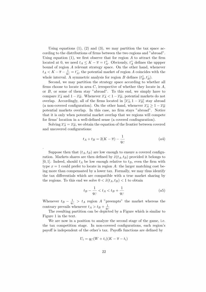
Using equations (1), (2) and (3), we may partition the tax space ac-cording to the distributions of firms between the two regions and ”abroad”.Using equation (1), we first observe that for region A to attract the firmlocated at 0, we need tA ≤ K − π = t+A. Obviously, t+A defines the uppperbound of region A relevant strategy space. On the other hand, whenevertA < K − π− 1

qC= t−A, the potential market of region A coincides with the

whole interval. A symmetric analysis for region B defines (t+B, t−B).Second, we may partition the strategy space according to whether all

firms choose to locate in area C, irrespective of whether they locate in A,or B, or some of them stay ”abroad”. To this end, we simply have tocompare xA and 1− xB. Whenever xA < 1− xB, potential markets do notoverlap. Accordingly, all of the firms located in [xA, 1 − xB] stay abroad(a non-covered configuration). On the other hand, whenever xA ≥ 1− xB

potential markets overlap. In this case, no firm stays ”abroad”. Noticethat it is only when potential market overlap that we regions will competefor firms’ location in a well-defined sense (a covered confiuguration).

Solving xA = xB, we obtain the equation of the frontier between coveredand uncovered configurations:

tA + tB = 2(K − π)− 1qC

(a4)

.Suppose then that (tA, tB) are low enough to ensure a covered configu-

ration. Markets shares are then defined by x̃(tA, tB) provided it belongs to[0, 1]. Indeed, should tA be low enough relative to tB, even the firm withtype x = 1 could prefer to locate in region A: the larger matching cost be-ing more than compensated by a lower tax. Formally, we may thus identifythe tax differentials which are compatible with a true market sharing bythe regions. To this end we solve 0 < x̃(tA, tB) < 1 to obtain

tB −1qC

< tA < tB +1qC

(a5)

Whenever tB − 1qC

> tA region A ”preempts” the market whereas thecontrary prevails whenever tA > tB + 1

qC

The resulting partition can be depicted by a Figure which is similar toFigure 1 in the text.

We are now in a position to analyze the second stage of the game, i.e.the tax competition stage. In non-covered configurations, each region’spayoff is independent of the other’s tax. Payoffs functions are defined by

Ui = qC(W + ti)(K − π − ti)

22

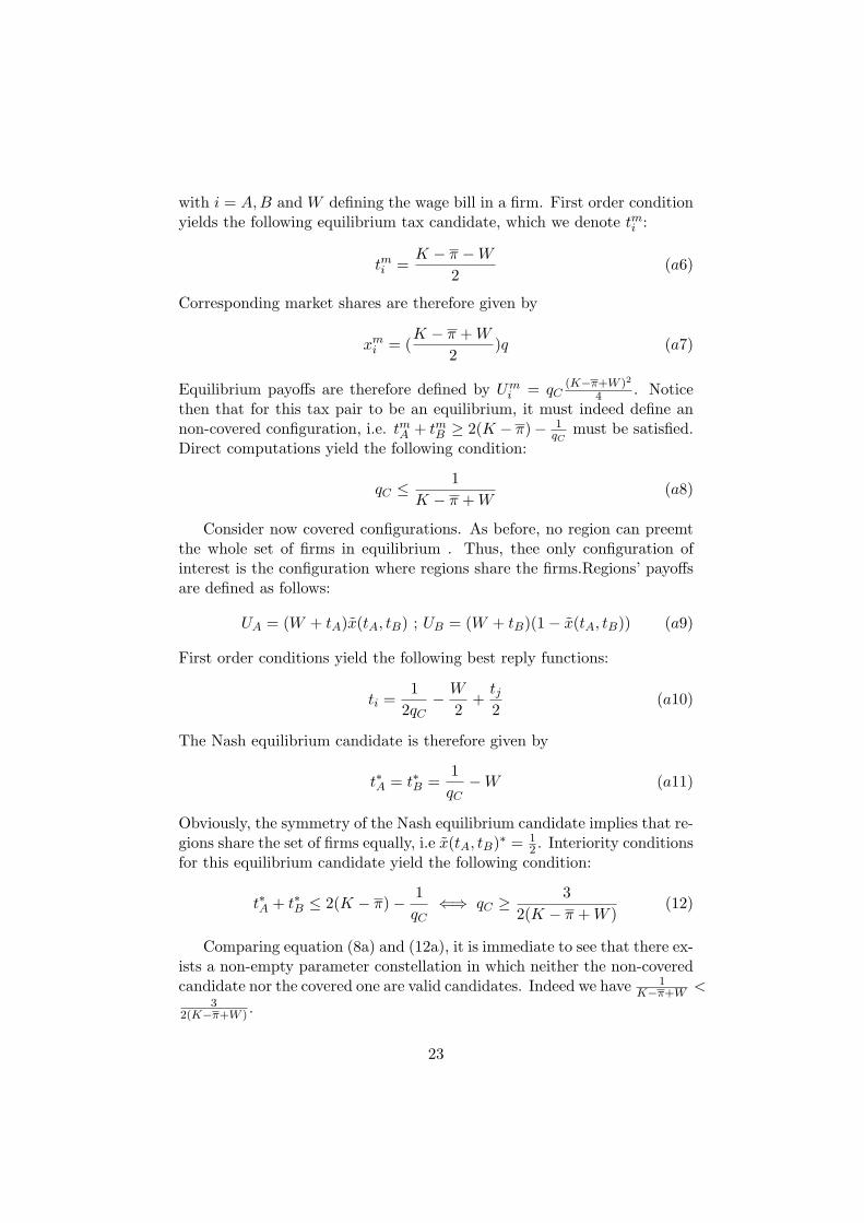
with i = A,B and W defining the wage bill in a firm. First order conditionyields the following equilibrium tax candidate, which we denote tmi :

tmi =K − π −W

2(a6)

Corresponding market shares are therefore given by

xmi = (

K − π + W

2)q (a7)

Equilibrium payoffs are therefore defined by Umi = qC

(K−π+W )2

4 . Noticethen that for this tax pair to be an equilibrium, it must indeed define annon-covered configuration, i.e. tmA + tmB ≥ 2(K − π)− 1

qCmust be satisfied.

Direct computations yield the following condition:

qC ≤1

K − π + W(a8)

Consider now covered configurations. As before, no region can preemtthe whole set of firms in equilibrium . Thus, thee only configuration ofinterest is the configuration where regions share the firms.Regions’ payoffsare defined as follows:

UA = (W + tA)x̃(tA, tB) ; UB = (W + tB)(1− x̃(tA, tB)) (a9)

First order conditions yield the following best reply functions:

ti =1

2qC− W

2+

tj2

(a10)

The Nash equilibrium candidate is therefore given by

t∗A = t∗B =1qC

−W (a11)

Obviously, the symmetry of the Nash equilibrium candidate implies that re-gions share the set of firms equally, i.e x̃(tA, tB)∗ = 1

2 . Interiority conditionsfor this equilibrium candidate yield the following condition:

t∗A + t∗B ≤ 2(K − π)− 1qC

⇐⇒ qC ≥3

2(K − π + W )(12)

Comparing equation (8a) and (12a), it is immediate to see that there ex-ists a non-empty parameter constellation in which neither the non-coveredcandidate nor the covered one are valid candidates. Indeed we have 1

K−π+W <3

2(K−π+W ) .

23

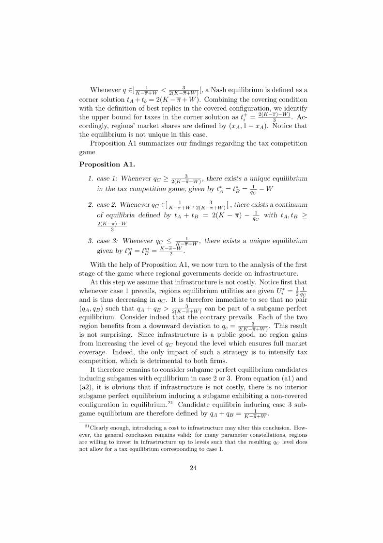
Whenever q ∈] 1K−π+W < 3

2(K−π+W ) [, a Nash equilibrium is defined as acorner solution tA + tb = 2(K −π +W ). Combining the covering conditionwith the definition of best replies in the covered configuration, we identifythe upper bound for taxes in the corner solution as t+i = 2(K−π)−W )

3 . Ac-cordingly, regions’ market shares are defined by (xA, 1 − xA). Notice thatthe equilibrium is not unique in this case.

Proposition A1 summarizes our findings regarding the tax competitiongame

Proposition A1.

1. case 1: Whenever qC ≥ 32(K−π+W ) , there exists a unique equilibrium

in the tax competition game, given by t∗A = t∗B = 1qC−W

2. case 2: Whenever qC ∈] 1K−π+W , 3

2(K−π+W ) [ , there exists a continuum

of equilibria defined by tA + tB = 2(K − π) − 1qC

with tA, tB ≥2(K−π)−W

3

3. case 3: Whenever qC ≤ 1K−π+W , there exists a unique equilibrium

given by tmA = tmB = K−π−W2 .

With the help of Proposition A1, we now turn to the analysis of the firststage of the game where regional governments decide on infrastructure.

At this step we assume that infrastructure is not costly. Notice first thatwhenever case 1 prevails, regions equilibrium utilities are given U∗

i = 12

1qC

and is thus decreasing in qC . It is therefore immediate to see that no pair(qA, qB) such that qA + qB > 3

2(K−π+W ) can be part of a subgame perfectequilibrium. Consider indeed that the contrary prevails. Each of the tworegion benefits from a downward deviation to qc = 3

2(K−π+W ) . This resultis not surprising. Since infrastructure is a public good, no region gainsfrom increasing the level of qC beyond the level which ensures full marketcoverage. Indeed, the only impact of such a strategy is to intensify taxcompetition, which is detrimental to both firms.

It therefore remains to consider subgame perfect equilibrium candidatesinducing subgames with equilibrium in case 2 or 3. From equation (a1) and(a2), it is obvious that if infrastructure is not costly, there is no interiorsubgame perfect equilibrium inducing a subgame exhibiting a non-coveredconfiguration in equilibrium.21 Candidate equilibria inducing case 3 sub-game equilibrium are therefore defined by qA + qB = 1

K−π+W .

21Clearly enough, introducing a cost to infrastructure may alter this conclusion. How-ever, the general conclusion remains valid: for many parameter constellations, regionsare willing to invest in infrastructure up to levels such that the resulting qC level doesnot allow for a tax equilibrium corresponding to case 1.

24

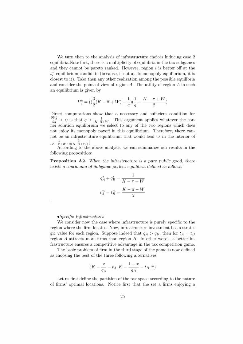
We turn then to the analysis of infrastructure choices inducing case 2equilibria.Note first, there is a multiplicity of equilibria in the tax subgamesand they cannot be pareto ranked. However, region i is better off at thet−i equilibrium candidate (because, if not at its monopoly equilibrium, it isclosest to it). Take then any other realization among the possible equilibriaand consider the point of view of region A. The utility of region A in suchan equilibrium is given by

U ca = ((

32(K − π + W )− 1

q)(

1q− K − π + W

2)

Direct computations show that a necessary and sufficient condition for∂Uc

A∂q < 0 is that q > 1

K−π+W . This argument applies whatever the cor-ner solution equilibrium we select to any of the two regions which doesnot enjoy its monopoly payoff in this equilibrium. Therefore, there can-not be an infrastrcuture equilibrium that would lead us in the interior of] 1K−π+W , 3

2(K−π+W ) [According to the above analysis, we can summarize our results in the

following proposition:

Proposition A2. When the infrastructure is a pure public good, thereexists a continuum of Subgame perfect equilibria defined as follows:

q∗A + q∗B =1

K − π + W

tmA = tmB =K − π −W

2.

•Specific InfrastructuresWe consider now the case where infrastructure is purely specific to the

region where the firm locates. Now, infrastructure investment has a strate-gic value for each region. Suppose indeed that qA > qB, then for tA = tBregion A attracts more firms than region B. In other words, a better in-frastructure ensures a competitive advantage in the tax competition game.

The basic problem of firm in the third stage of the game is now definedas choosing the best of the three following alternatives

{K − x

qA− tA,K − 1− x

qB− tB, π}

Let us first define the partition of the tax space according to the natureof firms’ optimal locations. Notice first that the set a firms enjoying a

25

positive surplus is region i is defined as follows :

xi = qi(K − π − ti) (a13),

for i = a, b.Accordingly, all firms choose to locate in one of the two regions (covered

configuration) whenever xA +xB ≥ 1. Solving this expression for tax rates,we define the frontier between covered and uncovered markets in the taxspace by the following relation:

tAqA + tBqB = (K − π)(qA + qB)− 1 (14)

Notice that the upper bound in the relevant tax domain firm region iis still given by K − π whereas the tax level ensuring that the potentialmarket coincides with the full market is given by K − π − 1

qi.

Let us then assume that regions’ markets overlap. The firm being in-different between the two regions, which we denote by x̂(tA, tB) solves bydefinition

K − π − x

qA= K − π − 1− x

qB.

We therefore obtain

x̂(tA, tB) =qAqB

qA + qB(

1qB

= tB − tA). (a15)

It then remains to check for the interiority conditions of market sharing,i.e. identify the conditions under which x̂(tA, tB) ∈ [0, 1]. Direct computa-tions yield:

x̂(tA, tB) ≤ 0 ⇐⇒ tA ≥ tB +1qB

x̂(tA, tB) ≥ 1 ⇐⇒ tB ≥ tA +1qA

We may now characterize the equilibrium distribution of the firms as afunction of the tax pairs. Replicating the analysis of the previous section,it is immediate to derive Monopoly equilibrium candidates for i = a, b as:

tmi =K − π −W

2with xm

i = qi(K − π + W

2) (a16)

We may then derive the feasibility condition for such an equilibrium byusing equation (a16). More precisely, we solve tmA qA +tmB qB ≤ (K−π)(qA +qB) − 1 for qA and obtain the interiority condition for the two regions tobehave as monopolist as:

qA ≤2

K − π + W(a17)

26

We characterize now a covered market equilibrium configuration. Usingthe definition of x̂(tA, tB) and equation (9), we characterize regions’ bestreplies as follows:

ti =tj −W

2+

12qj

; i, j = A,B

Accordingly, the unique Nash equilibrium is given

t∗i =1

3qi+

23qj

−W (a18)

Notice that markets shares in this equilibrium are defined by

x̂(tA, tB)∗ =qA + 2qB

3(qA + qB)(a19)

We now have to check for interiority conditions, i.e. solving

t∗AqA + t∗BqB ≤ (K − π)(qA + qB)− 1 (a20)

This equation can be re-expressed as

q2A(2− 3ZqB) + qA(qB(5− 3ZqB)) < 0 (a21)

where Z = (K − π + W ).Solving this expression for qA is not straightforward. However, in the

relevant domain of parameters, we obtain after some algebraic manipula-tions the following condition:

qA ≥5− 3qBZ +

√9− 6qBZ + 9q2

BZ2

−4 + 6Z= f(qB) (a22)

It is again a matter of computations to show that equations (a17) and(a22) are mutually exclusive. Accordingly, these two conditions define threemutually exclusive regions in the (qA, qB) space. Notice also that wheneverneither (a17) nor (a22) hold, the equilibrium is defined as continuum of taxpairs such that condition (a14) is satisfied, i.e. we have corner equilibria.These equilibria can be characterized as follows:

tcA = (tcBqB + (K − π)(qA + qB)− 1)1qA

(a23)

xcA = 1− (K − π)qB − tcBqB (a24)

Nash equilibrium in the tax game can thus be summarized through thefollowing Proposition:

27

Proposition A3. Suppose infrastructure are region’s specific, then theequilibria are given by:

1. Monopoly tax rates as defined by (a16) whenever qA ≤ 2K−π+W

2. Corner solutions as defined by (a23) whenever qA ∈ [ 2K−π+W , f(qB)]

3. Duopoly tax rates as defined by (a18) whenever qA ≥ f(qB)

Having characterized tax equilibria, we may now go backward in thegame tree to consider infrastructure choices. Using equations (a19) and(a20), we define equilibrium utilities in the covered equilibrium configura-tions as follows:

U∗i (qi, qj) = (

13qi

+2

3qj)

qj + 2qi

3(qi + qj)(a26)

A sufficient condition for ∂Ui∂qi

< 0 is qi, qj > 0. In other words, whateverthe other regions’ infrastructure, each region’s wishes to minimize its owninfrastructure. Notice that this implies that a pair (qA, qB) such that (a22)holds with strict inequality cannot be part of a subgame perfect equilibrium.This result may be surprising at first sight because by increasing qi, thisregion will manage to capture a larger share of the firm. However, this turnout to be very costly in terms of equilibrium tax levels. Accordingly, theregion prefers to keep qi ”small” to relax tax competition.

A similar analysis can be performed in the case of corner solutions,leading to the same conclusion: a region always wishes to reach the lowerbound of the domain defining corner solutions, whatever the equilibriumwhich is selected in the tax game. Accordingly, if a subgame perfect equi-librium exists it must be located in the domain where monopoly tax rateequilibria are defined. Using equations (a15), it is immediate to check thatany region’s utility is monotonically increasing in qi within the Monopolydomain. Accordingly with end up with multiple equilibria that take thefollowing form:

Proposition A4. When the infrastructure is a pure private good, thereexists a continuum of Subgame perfect equilibria defined as follows:

q∗A + q∗B =2

K − π + W

tmA = tmB =K − π −W

2.

Notice that in any of these subgame perfect equilibria, regions name thesame tax levels. However, they enjoy different market shares depending on

28

the levels of their infrastructure. Remark also that we may identify boundson the admissible domain of (q∗a, q

∗B). Specifically, arbitrarily small levels

for qi cannot be part of an interior. Indeed, the market share captured byfirm i in this equilibrium is so small that it will find it profitable to deviateto a larger qi that would enforce an equilibrium with covered configuratinonin the ensuing tax subgame.

29