A N D R I U S T O N K O N O G O V A S

S U M M A R Y O F D O C T O R A L D I S S E R T A T I O N

K a u n a s2 0 1 5

I N V E S T I G A T I O N O F P U L S A T I N G F L O W

E F F E C T O N M E T E R S W I T H R O T A T I N G

P A R T S

T E C H N O L O G I C A L S C I E N C E S , E N E R G E T I C S

A N D P O W E R E N G I N E E R I N G ( 0 6 T )

KAUNAS UNIVERSITY OF TECHNOLOGY

LITHUANIAN ENERGY INSTITUTE

ANDRIUS TONKONOGOVAS

INVESTIGATION OF PULSATING FLOW EFFECT ON

METERS WITH ROTATING PARTS

Summary of Doctoral Dissertation

Technological Sciences, Energetics and Power Engineering (06T)

2015, Kaunas

This scientific work was performed in 2009 – 2013 at the Laboratory of Heat

Equipment Research and Testing of Lithuanian Energy Institute.

Scientific supervisor:

Dr. Habil. Antanas Pedišius (Energy Technology Institute, Technological

Sciences, Energetics and Power Engineering – 06T).

Board of Energetics and Power Engineering Science field:

Prof. Dr. Habil. Stasys ŠINKŪNAS (Kaunas University of Technology,

Technological Sciences, Energetics and Power Engineering – 06T) – chairman;

Prof. Dr. Habil. Juozas AUGUTIS (Vytautas Magnus University, Technological

Sciences, Energetics and Power Engineering – 06T);

Prof. Dr. Gvidonas LABECKAS (Aleksandras Stulginskis University,

Technological Sciences, Energetics and Power Engineering – 06T);

Dr. Raimondas PABARČIUS (Lithuanian Energy Institute, Technological

Sciences, Energetics and Power Engineering – 06T);

Prof. Dr. Habil. Eugenijus UŠPURAS (Lithuanian Energy Institute,

Technological Sciences, Energetics and Power Engineering – 06T).

Official opponents:

Assoc. Prof. Dr. Audrius JONAITIS (Kaunas University of Technology,

Technological Sciences, Energetics and Power Engineering – 06T);

Prof. Dr. Habil. Vytautas MARTINAITIS (Vilnius Gediminas Technical

University, Technological Sciences, Energetics and Power Engineering – 06T).

The official defense of the dissertation will be held at 10 a.m. on 23rd April, 2015

at the public meeting of Board of Energetics and Power Engineering Science

field at the Session Hall in the Central building of Lithuanian Energy Institute

(Breslaujos st. 3, Room No. 202, Kaunas).

Summary of dissertation is sent out on 23rd March, 2015.

The dissertation is available in the libraries of Kaunas University of Technology

(K. Donelaicio st. 20, Kaunas) and Lithuanian Energy Institute (Breslaujos st. 3,

Kaunas).

KAUNO TECHNOLOGIJOS UNIVERSITETAS

LIETUVOS ENERGETIKOS INSTITUTAS

ANDRIUS TONKONOGOVAS

PULSUOJANČIO SRAUTO POVEIKIO MATUOKLIŲ SU

BESISUKANČIOMIS DALIMIS DARBUI TYRIMAS

Daktaro disertacijos santrauka

Technologijos mokslai, energetika ir termoinžinerija (06T)

2015, Kaunas

Disertacija rengta 2009 – 2013 m. Lietuvos energetikos institute, šiluminių

įrengimų tyrimo ir bandymų laboratorijoje

Mokslinis vadovas:

Habil. dr. Antanas Pedišius (Lietuvos energetikos institutas, technologijos

mokslai, energetika ir termoinžinerija – 06T).

Energetikos ir termoinžinerijos mokslo krypties taryba:

Prof. habil. dr. Stasys ŠINKŪNAS (Kauno Technologijos universitetas,

technologijos mokslai, energetika ir termoinžinerija – 06T) – pirmininkas;

Prof. habil. dr. Juozas AUGUTIS (Vytauto Didžiojo universitetas, technologijos

mokslai, energetika ir termoinžinerija – 06T);

Prof. dr. Gvidonas LABECKAS (Aleksandro Stulginskio universitetas,

technologijos mokslai, energetika ir termoinžinerija – 06T);

Dr. Raimondas PABARČIUS (Lietuvos energetikos institutas, technologijos

mokslai, energetika ir termoinžinerija – 06T);

Prof. habil. dr. Eugenijus UŠPURAS (Lietuvos energetikos institutas,

technologijos mokslai, energetika ir termoinžinerija – 06T).

Oficialieji oponentai:

Doc. dr. Audrius JONAITIS (Kauno Technologijos universitetas, technologijos

mokslai, energetika ir termoinžinerija – 06T);

Prof. habil. dr. Vytautas MARTINAITIS (Vilniaus Gedimino technikos

universitetas, technologijos mokslai, energetika ir termoinžinerija – 06T).

Disertacija bus ginama viešame energetikos ir termoinžinerijos mokslo krypties

tarybos posėdyje 2015 m. balandžio 23 d. 10 val. Lietuvos energetikos instituto

posėdžių salėje (Breslaujos g. 3, 202 kab., Kaunas).

Disertacijos santrauka išsiųsta 2015 m. kovo 23 d.

Su disertacija galima susipažinti Kauno technologijos universiteto (K.

Donelaicio g. 20, Kaunas) ir Lietuvos energetikos instituto (Breslaujos g. 3,

Kaunas) bibliotekose.

5

1. INTRODUCTION

Relevance of the dissertation work and the problem of scientific research

Air flow rate and velocity measurements are very important in scientific

investigations and in many manufacturing activities and environment protection

when ensuring proper conditions of occupational safety and health and

accounting of material and energetic resources. Conclusions of investigations in

air flow can be adopted in other flows, for example, natural gas and water. Flow

rate and velocity are the most popular characteristics in measurements.

Flow rate and velocity are usually measured using several types of meters.

In practice mostly meters with rotating rotors are used, rotation frequency of

which depends on the measured parameter (flow rate or velocity). Meters of such

kind are assigned to the tachometric meter class. Based on the principle of

operation, tachometric meters are classified into velocity (vane, turbine and

mechanical anemometers) and positive displacement meters. Tachometric meter

measures number of rotations of the sensor, which respectively is proportional to

the volume of the flow and/or rotational frequency, which is proportional to flow

rate velocity. Advantages of the tachometric meters are the following: wide

dynamic range of measurement and high accuracy (unfortunately, it is achieved

only under excellent flow conditions); disadvantages: low sensitivity and high

inertia.

The objects of the work were tachometric meters of the following types:

– turbine flow meter and cup anemometers;

– positive displacement (rotary) flow meters.

It is worth noting that turbine gas meters are ones of the most important

measuring devices for natural gas flow rate use. They measure up to 70 % of

total natural gas use, which is currently 2.5 billion m3 per year. Also these meters

are widely used as basic measurement means in reference facilities for recreation

of air (gas) volume and flow unit values and then transferring it to working

standards or meters. In the measurement range from 200 to 9700 m3/h of

Lithuania’s air (gas) volume and flow unit standard, five turbine meters are used.

Usually turbine flow rate meters are operating under unstable conditions, i.e.,

when flow rate, velocity and, sometimes, direction of the flow change. Usually

flow change is periodical, i.e., the meter operates when the flow is pulsing.

Air velocity meters usually work under high wind turbulence, which could

reach several tens of percent. Their operation in a pulsating flow is affected by

analogous factors as in the case of turbine flow rate meters. In the case of wind

pulsations, the meters, due to their inertia, are not able to react to sudden changes

of air flow velocity. Variation regularity of dynamic errors generated by these

meters is especially important when measuring non-stationary wind speed and

calculating wind energy from these measurements. The main difference between

mechanical air velocity meters and turbine gas flow rate meters is the form and

6

the size of an impeller that determine differences between aerodynamic forces

and, respectively, response and dynamic errors.

The main parameters of flow pulsations are their frequency, amplitude and

law of pulsation. These parameters have great influence on pulsation effect to

readings of meters and measurement accuracy. However, until now all

investigations concentrated on determination of a dynamic error when flow

pulsates according to simple laws (usually cosine). However, usually the

measured flows pulsate according to various complex laws, which differ from

cosine. Also until now there was no any method for modeling of meter operation

in a pulsating flow that varies according to any law of pulsation.

The aim of the dissertation

Investigate influence of air (gas) flow pulsations on operation and errors of

tachometric meters (turbine meters, positive displacement flow meters and cup

anemometers).

Tasks of the investigation

In order to achieve the objective the following tasks should be solved:

– Prepare an experimental method for determination of inertia time

constant of tachometric meters and investigate their inertia

characteristics;

– Prepare a numerical method for evaluation of the response and

dynamic error of turbine flow meters and cup anemometers in a

pulsating flow;

– Investigate influence of flow, which pulsates under simple

(rectangular, triangle and cosine) and complex (met in practice)

laws on response and dynamic error of turbine flow meters and

generalize the obtained dependences;

– Investigate the influence of wind pulsations on response and

dynamic error of cup anemometers and generalize the obtained

dependences;

– Experimentally investigate influence of pulsations on dynamic error

of rotary gas meters;

– Investigate influence of oscillating and reversal pulsing flow on

performance of turbine flow meters;

– Prepare recommendations for application of the results of the work

in practice.

Practical value of the work

Recommendations for elimination of dynamic errors of the meter working

in a pulsating flows are prepared.

7

Scientific novelty of the work

– A new method for determination of the rotor’s inertia time constant

of tachometric meters according to its step response was created.

This method assess the influence of current and excess frequency of

rotor’s rotation on time constant;

– A new numerical method was created for modelling of the response

and dynamic error of turbine flow meters and cup velocity

anemometers in a flow, which pulsates under any law. Patterns of

the response and dynamic error dependencies on pulsation

parameters applying newly created dimensionless variables were

generalized.

Defensive statement

The following statements serve as defensive statements:

– Time constant of tachometric meters varies during the response and

depends not only on the final but also on the excessive frequency of

the rotor rotation. Initial frequency does not influence the character of

the change of time constant;

– Dynamic error of turbine flow meters is influenced by amplitude,

frequency and law of pulsation. Influence of frequency of pulsation

occurs at 0.1 Hz, while at increase to 1 Hz due to inertia of meter

readings in all cases their variation converges to sine pattern. At 2 Hz

dynamic error reaches its limit value and remains constant. Limit

value depends on law and amplitude of pulsation, which increase this

value by quadratic law;

– Dynamic error of cup anemometers is determined by the minimal and

maximal values of wind speed, pulsation frequency and coefficients

which settle the decreasing rate of the velocity pulsation amplitude

and frequency. Effect of frequency and amplitude of pulsation is

similar to the turbine flow meters, however, the dynamic error of cup

anemometers is negative when pulsation frequencies are lower than

0.01 Hz, and decreasing rate of the velocity pulsation amplitude is not

equal;

– Dimensionless dynamic error of the turbine flow meters and

mechanical cup anemometers with uncertainty ± 7 % summarises by

exponential dependence under any law of pulsation;

– Influence of flow pulsations on the dynamic error of rotary flow

meters is insignificant;

– Dynamic error of turbine gas meter in oscillating and reversal pulsing

flow is generalized by parameter, which describes flow rate

displacement in time.

8

2. EQUIPMENT AND METHODS OF EXPERIMENTAL

INVESTIGATIONS

Experimental investigations of tachometric meters’ (further – TM)

response to sudden flow changes were carried out using a test facility, the

principal scheme of which is shown in Fig. 2.1.

Fig. 2.1 Test facility for investigation of inertial forces of tachometric meters. 1 – meter

under test; 2 – pneumatic valves; 3 – Venturi type flow meter; 4 – fans with adjustable

speed; 5 – thermometers

The test facility consists of two aerodynamic tubes (A and B), each of

which is separated by a pneumatic valve. In each tube air flow is created,

controlled and measured separately, depending on the selected sudden air flow

rate decrease or increase in the investigated TM. A sudden change of flow rate

(velocity) in tube C, where the investigated TM is installed, is reached using

pneumatic valves, which change the value of the initial flow rate (velocity) in

tube A to the value of the final flow rate (velocity) in tube B. When the valves

are switched, synchronic registration of the frequency of pulses of the

investigated TM and the time, during which the impulse frequency settles, is

started.

2.1. Experimental method for dynamic error determination

Investigations of the effect of a flow that pulsates under complex laws of

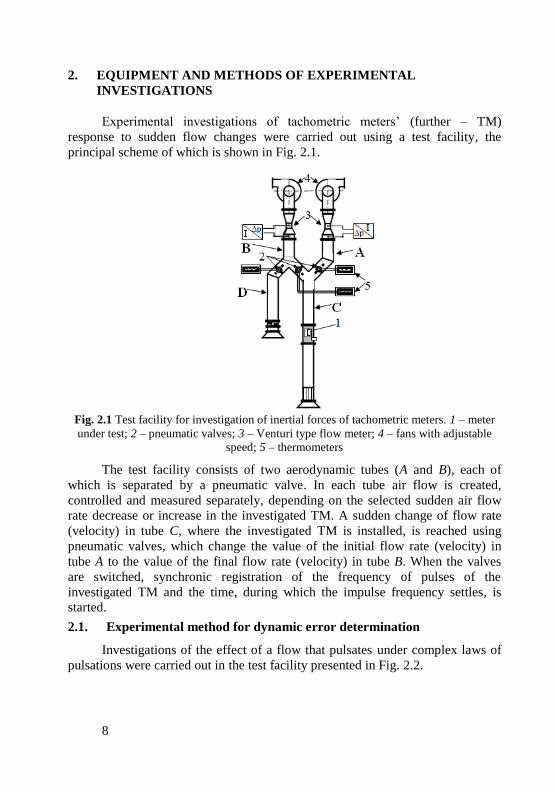
pulsations were carried out in the test facility presented in Fig. 2.2.

9

Fig. 2.2 Experimental test facility for investigation of dynamic error of flow meters. 1 –

compressor; 2 – receiver; 3 – pressure regulator; 4 – turbine flow meter; 5 – acoustic

filter; 6 – turbine flow meter; 7 – pressure regulator

The peculiarity of this facility is that a compressor is installed instead of a

fan, and it ensures the necessary air flow; also a pressure regulator is installed

that creates pulsations with varying patterns.

Reference flow was measured using a rotary gas meter (further RGM)

that had been installed in front of the investigated turbine gas meter (further –

TGM). A pressure regulator was installed at the end of the measuring section to

create flow pulsations. In order to simulate pulsations of various forms, a branch

with an electromagnetic valve, which was controlled manually as well as using

software, was installed. The dynamic error of the investigated TGM was

determined by comparing the readings of this meter to the readings of the

reference RGM.

During the investigation, flow pulsation values were determined

according to the measured differential pressure pulsations and the reference flow

value. It was assumed that an instantaneous flow rate was proportional to square

root of differential pressure ip in reference meter. The data were processed

in the following order:

– array of values of differential pressure Δpi for one period of

pulsation is determined;

– root values ip of every member from the selected array are

calculated. The absolute pressure value is selected since the flow

often changes the direction under the regulator’s operation;

– the mean value of the array avgip is calculated;

– the array of dimensionless flow rate values ip

avgi

i

ip

ppSIGN

is calculated.

This method was chosen since there were no technical tools to measure

instantaneous flow rate values.

1 5 3 2 4 7 6

10

3. METHODS FOR DETERMINATION OF ROTATIONAL INERTIA

TIME CONSTANT OF TACHOMETRIC METERS

The most important characteristic of any system that operates under

variable external effect is time constant. This parameter – sometimes called

inertia index – describes the system’s response and nature of the effect. Time

constant is a characteristic parameter of a non-stationary process system, to

which linear differential equation of the first order can be applied:

tukty

dt

tdy ; (3.1)

Here: τ – time constant s; y(t) – response; u(t) – input signal; k – conversion

factor.

To determine the time constant, experimental results of the meters’ step

response to a sudden flow rate change were used by applying the following two

methods:

– “37 %” method, which is known and used widely;

– A newly created method based on a detailed mathematical analysis

of the response curve.

In the first method, an exponential change of the signal was assumed

according to equation:

t

eyty )0()( . (3.2)

It was assumed that the time constant remains the same during the entire

time of the response. Regardless of the methodology of the task solution, the

time constant was assumed to be the main parameter of the TM rotor, although

for the TM this condition cannot be fulfilled or can be fulfilled partially.

Ω0

tt = T t

0,368∙

Ω

0

Fig. 3.1 Determination scheme of inertia time constant

Fig. 3.1 presents the scheme of determining inertia time constant applying

the “37 %” method, according to which the time constant is defined as time

t = τ

Ω0

Ω = 0.368∙Ω0

t

11

during which dimensionless relative rotational frequency changes from the

initial value 0 = 1 to value = 0.368·0.

Relative rotational dimensionless frequency can be described using the

following equation:

t

galpr

gale ; (3.3)

here ω – current TM rotor rotational frequency Hz; ωin and ωfin – initial

and final TM rotor rotational frequency respectively Hz; t – time s.

The second method was applied assuming that the time constant is

varying during the transition process.

In order to determine the dependency of time constant on current

rotational parameters, the following method was applied:

– The response dependency in time of the investigated meter was

approximated by a 6th degree polynomial

66

221 tatataln ; (3.4)

– and from dependencies of equation (3.3) and equation (3.4) the

time constant expression was obtained:

5621

1

tataa

. (3.5)

This method can be applied to determine the time constant for all types of

tachometric meters.

3.1. Method for determination of response and dynamic error of turbine

meters

The scheme of dynamic error formation is shown in Fig. 3.2.

The finite difference method was applied to this modelling. Distribution

of the meter rotor’s rotations frequency in time equal to pulsation period was

calculated

f/t 10 ; (3.6)

here f – frequency of flow rate pulsation Hz.

Time Δt0 was expanded into a large number of time intervals Δti (Δti<<

Δt0). The initial frequency iin in every time interval Δt0 was calculated

according to the final frequency 1

ifin known from calculation in the previous

time interval Δti-1 by evaluating the following condition

12

1

ii finin (3.7)

and using experimentally determined response of the meter to a sudden

change of flow rate applying Equation 3.7.

Fig. 3.2. The scheme of dynamic error formation: 1 – real flow rate; 2 – flow rate

corresponding to the meter rotations; 3 – unregistered amount of gas; 4 – registered excess

amount of gas

Flow rate Qi was calculated according to its selected dependence Qi = f(t)

and was assumed to be constant during the entire time interval ti, i.e., the

selected smooth curve of the flow rate change was modelled in a manner of

stepwise dependence (Fig. 3.3).

Fig. 3.3. Substitution of flow rate curve (1) to a stepwise pattern (2), with the length of a

step ti

Relative frequency fin/in was calculated according to dependence:

ii infinin/fin / . (3.8)

For modelling a specific meter, the time constant value was determined by

the experimental investigation results of this meter.

Values and equations used for calculations are presented below:

– The passing flow rate according to the meter readings:

impm k/Qi

; (3.9)

Flo

w

Time

4 3

+ +

– – 1 2

13

– Average real flow rate Qavg during time ∆t0:

n/QQ iavg ; (3.10)

– Average flow rate according to the meter readings:

n/QQisk avgavg ; (3.11)

– Dynamic error:

avgavgavg QQQsk (3.12)

The provided equations make the mathematical model of the process

under consideration.

Contrary to TGM, mechanical air velocity meters (further – MAM)

operate in open atmospheric flows usually under strong turbulence that could

reach several tens of percent. In order to model such complex form fluctuations

of wind velocity, the following parameters of pulsations were determined:

– Minimal vmin and maximal vmax velocity values;

– Wind velocity pulsation frequency f;

– Coefficient kv (kv ≥ 0), which defines the decrease rate of the

velocity pulsations amplitude (the amplitude decreases according to

an arithmetic progression) within one cycle of pulsation. At kv = 0

the value of the velocity amplitude remains constant. When the

value of this parameter increases (kv > 0), the decrease rate of

pulsation amplitude values becomes faster;

– Coefficient kt (kt ≥ 0), which defines the decrease rate of the velocity

pulsations frequency (frequency also decreases according to

arithmetic progression) within one cycle of pulsation. At kt = 0 the

value of the velocity frequency remains constant. As the value of

this parameter increases (kv > 0), the decrease rate of pulsation

frequency values becomes faster;

– Number of peaks in one impulse of pulsation.

While modelling air velocity pulsations, it was assumed that there would

be eight peaks in one pulsation. After choosing the maximum and minimum air

velocity values, wind pulsations corresponding to laws, met in practice, were

modelled.

3.2. Methods for summary of the results

The obtained results were summarised applying dimensionless parameters

provided in Table 3.1.

14

Table 3.1. Dimensionless parameters

Parameter name Expression

Dimensionless amplitude of gas

flow rate pulsation avg

a

avg Q

QQ

Q

QQ

2

- minxm

Dimensionless amplitude of air

velocity pulsation avg

minmax

v

vvv

Dimensionless flow rate avgQ/QQ avgmaxmax Q/QQ avgminmin Q/QQ

Dimensionless amplitude of

pulsation of meter readings avg

minmax

q

qqq

2

Dimensionless relative

amplitude of pulsation of meter

readings

Q/qqrel

Dimensionless frequency of

flow rate pulsation ff

Dimensionless time tft

Dimensionless dynamic error lim/

The limit dynamic error value lim depends only on the law of pulsation

and dimensionless pulsation amplitude Q and can be described using the following equation:

2QC~ alim . (3.13)

Analysing an oscillating and reversal pulsing flow using the method under

consideration when the flow changes its direction periodically, instead of

dimensionless amplitude, it is convenient to introduce a new dimensionless

parameter C, which describes displacement of the pulsating flow rate in respect

of time axis – in fact, dimensionless flow rate displacement in respect of 1 and is

related to dimensionless amplitude Q :

QC

1; avgminmax Q/QQC 2 ; minQC 1 ; 1 maxQC (3.14)

It can be applied simulations in the case of reversal pulsing flow. Values

С ≥ 1 correspond to single direction pulsations, 0 ≤ С < 1 correspond to double

direction pulsations (reversal pulsing flow), case С = 0 corresponds to a

oscillating flow which average flow rate value is zero.

15

4. RESEARCH OF RESULTS OF INERTIA OF TACHOMETRIC

FLOWMETERS

During analysis of measurement results of the tachometric meter response,

it was determined that under the same boundary conditions, the response time of

different type of meters depends directly on physical characteristics of the meter

(mass, size) and on the material of which the meter’s impeller or rotor is made

and its size. Moreover, the response time due to torque depends directly on the

final flow rate value Qfin.

The manner of the rotary meter response differs basically from the turbine

flow rate and cup air velocity meters response. Measuring of the rotary meter

principle is based on periodic displacement of the measured air flow from the

chambers. So, in the case of a sudden change of flow rate, frequency of rotary

meter rotor determines the initial flow rate value.

Applying method “37 %”, the averaged inertia time constant was

determined according to the measured responses of the turbine flow rate meters

to a sudden flow rate change. As in the case of the response, the final flow rate

value also greatly affected the time constant. Three different types of meters

have been investigated. The time constant dependencies of the analysed meters

on the final flow rate Q are shown in Fig. 4.1.

Time constant of a turbine flow meter in gas with fixed physical

properties (first of all density and viscosity) is described by the following

dependence:

nfinQ

B

100; (4.1)

here Qfin – final flow rate m3/h.

Fig. 4.1. Inertia time constant τ dependence of three types of turbine meters on the final

flow Q; a – meter 1; b – meter 2; 3 – meter 3

Coefficient C and indicator n in this equation can be determined pretty

accurately and easily applying a semi-experimental method. In all cases, degree

indicator n is more or less close to 1. Density ratio of metal and plastic impellers

ρmet/ρpl is very close to the ratio of inertia time constant τmet/τpl of these impellers.

This means that time constant τ is inversely proportional to the final flow rate

and directly proportional to the moment of inertia I of the turbine impeller.

16

During the investigation, analysis of the measured response of the meter

was performed. Fig. 4.2 demonstrates a typical change of dimensionless

frequency Ω of a tachometric meter in time. The following presentation of the

results allows better understanding the nature of the meter’s response. The

straight line means that the meter’s response varies in time exponentially with a

constant exponent, while the time constant remains the same during the response

process. The appearance of curves means that the exponent and the time constant

changes during the transitional process. Thus, if the curve is bent downwards, the

exponent value in this field decreases, and the time constant increases.

Fig. 4.2 Dependence of the dimensionless relative frequency of the turbine meter on time

when the flow rate starts decreasing from Qin = 700 m3/h to (1–6) – Qfin = 0; 50; 100; 200;

300; 500 m3/h

A detailed analysis of tachometric meters performance was carried out

analysing their response to a sudden change of the flow rate. A typical

dependence of the time constant on excessive frequency (the difference between

the current and the final rotational frequencies) is shown in Fig. 4.3 (a) for low

excessive frequency, and in Fig. 4.3 (b) for high excessive frequency. In the first

case, results for increasing as well as for decreasing flow rate change are

provided.

Fig. 4.3. Time constant dependence of the turbine meter on the difference between the

current and final frequencies. a:1–3 Qin = 50 m3/h, Qfin = 500; 300; 200 m3/h; 4 – 6

Qin = 700 m3/h, Qfin = 500; 300; 200 m3/h; b – Qin = 700 m3/h; 7–9 Qfin = 100; 50; 0 m3/h

Analysis of Figure 4.3 shows that time constant changes significantly

during the response process, and the change is basically non-linear. The average

value of the time constant is higher when the flow rate change is increasing (Fig.

17

4.3 1–3) compared to the case when the flow rate change is decreasing (Fig. 4.3

4–6). The value of the time constant starts increasing when the final value of the

flow rate approaches the lower measuring boundary of the meter (Fig. 4.3 7–9).

When the final value of the flow rate approaches 0, the value of the time constant

is increasing exponentially.

For different values of initial flow rate and the same values of final flow

rate (Fig. 4.3, 1 and 4; 2 and 5; 3 and 6), the point of intersection of the time

constant coincides within the accuracy boundaries. This means that the initial

flow rate value does not influence the time constant.

While analysing changing of the time constant of the cup air velocity

meters, it was observed that non-monotonous dependence manner is related to

different effect of influencing factors. Aerodynamic forces of the flow accelerate

transition process; however, the effect of stopping factors is determined by

parameters of the transition process that are difficult to name because of great

uncertainty. At low excessive frequencies, dispersion of results grows

significantly. This is determined by decrease in the difference of the measured

frequencies and by increase of the uncertainty of the results. For the final

velocity, inertia time constant depends on the values of the final velocity and is

inversely proportional to it.

The change manner of time constant corresponds to the change manner of

rotational frequency. When the rotational frequency decreases and approaches

the final value, the time constant increases. When the final rotational frequency

increases, increase of the time constant slows down. When the values of the

rotational frequency are high, the increase of the time constant stops and

indicators of its decrease appear.

Response characteristics of the chamber flow rate meters to a sudden flow

rate change are similar to analogous characteristics of the turbine flow rate and

cup air velocity meters, and the same methods for summary of the results as in

the case of turbine meters can be applied using experimentally determined

dependences of change of the inertia time constant of the meters that have

several peculiarities.

5. MODELLING RESULTS OF TURBINE METER RESPONSE AND

DYNAMIC ERROR

Investigations of turbine meter response and dynamic error were carried

out when the flow pulsated according to simple (cosine, rectangular, triangle)

and complex (that occur in practice) laws. Each complex law was obtained as a

sum of elementary cosine pulsations at various amplitudes and frequencies.

Equations and forms of such pulsations are shown in Table 5.1.

At low frequency (0.01–0.05 Hz), there was practically no inertia, the

meter was able to follow even sudden flow changes, and its readings differed

only slightly from the real flow value. When the frequency increased to 0.5 Hz,

18

inertia was quite strong; however, the meter reacted to the flow change even at

low amplitude. At frequency that reached 10 Hz for calculation conditions, the

meter was not able to follow flow changes and its readings were practically

constant and higher than the average flow rate value.

In all cases, the meter readings vary at the same frequency as the flow rate;

however, phase displacement and amplitude decrease is apparent. For triangular,

cosine and complex laws of pulsation, the meter readings change according to

cosine law when pulsation frequency increases. Maximum and minimum of the

meter readings are displaced in time in respect of the flow rate maximum and

minimum and are reached when the meter reading equals to the instantaneous

real flow rate. For rectangular law of pulsation, the meter readings vary

according to complex exponential law. Maximum and minimum of the readings

are reached during a sudden change of the flow rate. In all cases the bigger the

amplitude of the meter readings, the bigger the amplitude of flow pulsation.

Dynamic errors and dimensionless amplitudes of the meter reading

pulsations considering the flow rate pulsation frequency were calculated for all

analysed laws of pulsations. Dependencies of dynamic error on frequency and

amplitudes flow pulsation are shown in Fig. 5.2 (rectangular law of pulsation)

and Fig. 5.3 a (complex law No. 1 of pulsation see Table 5.1). The following

common dependences can be seen. At low frequencies f < (0.01–0.001) Hz,

dynamic error is practically zero. When the frequency values exceed the

indicated values, the error increases till a certain limit value that depends on flow

pulsation law and amplitude.

The obtained results coincide with the results provided in [1]. However,

document [1] does not indicate characteristics of the meter inertia, and the

obtained results are only for a rectangular law of flow pulsation.

Table 5.1. Modelling of flow pulsations according to complex law

No. Pulsation law Form of

pulsation

Coeff.

Сa in

Eq

(2.14)

Coeff.

k in

Eq.

(5.4)

1 Q =1+ nomQ ·cos(2·π·t·f) – 0.09 nomQ ·cos(4·π·t·f) + 0.07

nomQ ·cos(6π·t·f)) - 0,04 nomQ ·cos(8π·t·f) 0, 60

1, 00

1, 40

0 50 100

44.24 5.8

2

Q =1+ nomQ ·cos(2·π·t·f)- 0,25 nomQ ·cos(4π·t·f) + 0.09 nomQ

·cos(6·π·t·f) - 0,05 nomQ ·cos12π·t·f) + 0.07 nomQ ·cos(14π·t·f)) -

0,04 nomQ ·cos(18π·t·f)

1

0, 60

1, 00

1, 40

0 50 100

42.71 5.2

3 Q =1+2/3 Δ nomQ ·cos(2·π·t·f)+1/2 nomQ ·cos(4π·t·f) -1/4

nomQ cos(8π·t·f)

1

0 ,7 5

1 ,0 0

1 ,2 5

0 5 0 1 0 0

48.93 5.7

4 Q =1+4/5 nomQ ·cos(2·π·t·f)-1/4 nomQ cos(8π·t·f) + 1/7

nomQ ·cos(16π·t·f) – 1/12 nomQ ·cos(20·π·t·f)

1

0, 75

1, 00

1, 25

0 50 100

38.26 5.1

19

5

Q =1+ nomQ ·cos(2·π·t·f)-0.35 nomQ ·cos(6π·t·f) + 0.25 nomQ

·cos(28π·t·f) – 0.09 nomQ ·cos(46·π·t·f) – 0.05

nomQ ·cos(96π·t·f) + 0.07 nomQ ·cos(120π·t·f)) – 0.04

nomQ ·cos(150π·t·f)

1

0, 75

1, 00

1, 25

0 50 100

35.60 5.4

6

Q =1+ nomQ cos(2·π·t·f)-0.35 nomQ cos(4π·t·f) + 0.25 nomQ

·cos(14π·t·f) – 0.09 nomQ ·cos(22·π·t·f) – 0.05 nomQ cos(48π·t·f)

+ 0.07 nomQ cos(60π·t·f)) – 0.04 nomQ cos(76π·t·f)

1

0,60

1,00

1,40

0 50 100

34.49 5.2

7

Q =1+ nomQ cos(2·π·t·f)- 0.25 nomQ cos(6π·t·f) + 0.09·

nomQ cos(10·π·t·f) – 0.05 nomQ cos(24π·t·f) +

0.07 nomQ cos(30π·t·f)) – 0.04 nomQ cos(38π·t·f)

1

0, 75

1, 00

1, 25

0 50 100

59.86 4.7

Fig. 5.1. Response of the turbine meter on flow pulsation at different frequencies

pulsations, flow when flow rate pulsates according to complex law No. 6 (see Table 4.1).

a – f = 0.01 Hz; b – f = 0.05 Hz; c – f = 0.1 Hz; d – f = 0.5 Hz, e – f = 10 Hz

Calculation results of the pulsation amplitude of rotational frequency of

the meter rotor, concerning the flow rate pulsation frequency, are provided in

Fig. 5.3 b at complex flow rate pulsation frequency No. 1 (Table 5.1)

respectively to various pulsation amplitudes of flow rate frequency. The

pulsation amplitudes of dynamic error and meter readings correlate with each

other depending on flow rate pulsation parameters. When the flow rate pulsation

amplitude increases, pulsation amplitude of the meter reading also increases.

When flow rate pulsation frequency f increases, the response amplitude

decreases, and retardation according to phase increases.

20

Fig. 5.2. Dynamic error dependence on flow pulsation frequency at different pulsation

amplitudes and rectangular law. 1, 2, 3 – Q = 0.25; 0.35 and 0.5 respectively

Summarising the obtained results, it is evident that at pulsation frequency

approx. (1–2) Hz, dynamic error reaches the limit value and stops increasing.

Within the field or error limit value, the meter readings practically do not

change, and inertia characteristics of the meter have no influence on dynamic

error. This frequency increases coherently when the law of flow rate pulsation

changes from triangle to rectangular. When the amplitude increases, the

frequency limit value also increases. For more inert meters (higher values of time

constant), the increase areas of the error curve move towards the lower

frequencies, i.e., the limit value is reached earlier; for less inert meters, the

process is the opposite. The meter’s inertia decreases with decreased friction in

bearings, better aerodynamics of the meter, decreased mass of the meter’s

impeller and increased gas pressure.

21

Fig. 5.3. Dynamic error of a turbine meter (a) and pulsation amplitude of the meter’s rotational frequency (b) when the flow rate pulsates according to complex law No. 1.

1–4 Q = 0.5; 0.35; 0.25 and 0.1 respectively

Fig. 5.4 shows dependence of the limit dynamic error of the meter on

dimensionless amplitude values.

Fig. 5.4. Dynamic error limit value dependence on the law of the flow pulsation: 1, 2 and

3 – rectangle, cosine and triangle law’s respectively

It can be seen that in all cases at any law of pulsation, this dependence on

amplitude is quadratic and determined by Equation (2.14). The biggest error is

obtained for rectangular law of flow pulsation. For cosine law the error is two

times lower. The minimal error value is obtained for triangle law of pulsation;

however, it is close to values obtained for the cosine law. Quadratic dependency

of the dynamic error on change amplitude remains at high amplitudes (> 10 %)

and other ( 1 Hz) frequencies.

Analysis shows that results of the dynamic error can be summarised using

dependencies of dimensionless dynamic error on dimensionless parameter f .

Fig. 5.5 Summarised dynamic error dependence on dimensionless flow pulsation

frequency at different pulsation amplitudes. Qavg= 400 m3/h; 1–5 – ΔQ = 0.05; 0.1; 0.25;

0.35; 0.5; 6 – approximation curve. a – cosine, b – triangle law of flow pulsation

a b

22

Fig. 5.6 Amplitude dependencies of summarized dynamic error of the turbine meter and

the meter reading pulsation. a and b – amplitude dependencies of dynamic error and of

readings pulsation on flow rate pulsation frequency; c and d – relation between

amplitudes of dynamic error and readings pulsations. 1 – flow rate pulsations according to

law No. 1; 2 – flow rate pulsations according to law No. 5 (see Table 5.1)

Fig. 5.6 shows summarised (dimensionless) turbine flow rate meter

dynamic errors and amplitude dependencies of rotational frequency pulsation

of the rotor on flow rate pulsation frequency when they change according to laws

No. 1 and 5 (Table 4.1) and dependencies that demonstrate relation between

parameters and q .

Calculations were performed for the turbine meter with a metal impeller at

values 0.05; 0.1; 0.25; 0.35 and 0.5 of relative flow rate pulsation amplitude Q .

Dimensionless dynamic error of the meter depends only on dimensionless

pulsation frequency f .

Fig. 5.7 Dimensionless dynamic error of the turbine meter at the analysed complex

pulsation laws and limit values of coefficient k: 1 – kmin = 4.7; 2 – kmax = 5.8; 3 – kavg = 5.2

23

It changes exponentially and can be summarised by the following equation

(see Fig. 5.7):

fke 1 . (5.1)

This equation can be applied to any other turbine flow meter given that the

inertia constant of the meter is known.

Coefficient k values at various laws of pulsations are provided in Table

5.1. Constant k values considering the law of flow rate pulsation vary in range of

(4.7–5.8). As can be seen in Fig. 5.7, difference between results at limit k values

is not significant. Thus, with uncertainty that does not exceed ±7 average k

value kvid = 5.2 can be used for all analysed complex laws of pulsation.

6. MODELLING RESULTS OF CUP ANEMOMETER RESPONSE

AND DYNAMIC ERROR

The method used for the turbine meters was applied for calculation of

response and dynamic error of the cup air velocity meter. The only difference

was that in case of the turbine meters, the inertia time constant was assumed to

depend only on the final flow rate or the final rotational frequency. In case of the

determining time constant of velocity meter influence of not only the final

frequency but also of excess (difference between the current and the final)

frequency value were evaluated. These dependencies were described by linear

expressions.

The calculation results of the investigated anemometer’s response to the

modelled wind velocity fluctuations are shown in Fig. 6.1 at the following

conditions: vmax=20 m/s; vmin = 5 m/s; kV =0.5; kt = 0.25; general pulsation

frequency (0.01 ÷ 10) Hz.

Fig. 6.1. Response of the cup velocity meter to wind fluctuations. 1 – instantaneous wind

velocity; 2 – average wind velocity; 3 – response of the air velocity meter. a, b, c, d

f = 0.01; 0.2; 0,5; 20 Hz respectively

At small pulsation frequency values ≤ 0.01 Hz, the cup velocity meter

does not show rotational inertia (the same as in the case of the turbine flow rate

meters); thus, it accurately repeats the air velocity pulsations. Also at increased

pulsation frequency, the meter is not able to follow the real velocity value, and

the response of the meter becomes a straight line that is higher than the average

flow rate value.

24

Fig. 6.2. Modelling results of dynamic error of the cup anemometer at kt = 0.5 and vmax =

10 m/s. a vmin = 1 m/s; 1–3 – kv = 0.1; 0.5 and 1 respectively; b 1–2 – vmin = 7.5 m/s, kv =

0.5 and 1 respectively; 3–5 – vmin = 1 m/s kv = 0.1; 0.5 and 1 respectively

Numerical modelling results of the dynamic error and the meter’s response

for flow pulsation at parameters kv = (0.1; 0.5; 1); kt = 0.5 are shown in Fig. 6.2.

Manner of the shown dependencies is the same as for case of turbine gas meter.

At small pulsation frequencies, the influence of inertia is practically non-

existent, and the dynamic error is close to 0. When the frequency increases, the

dynamic error also starts increasing until its limit value. As the frequency further

increases, the rotational frequency of the meter’s rotor becomes constant, and the

dynamic error ceases to change. The character change of the relative swing of

the meter readings corresponds to the character change of the dynamic error;

however, they are of opposite directions.

Contrary to the turbine flow rate meters, dynamic errors and curves of the

dimensionless amplitude layer out at different values of coefficient kv. Moreover,

separate curves intersect again. This can be explained by influence of an average

velocity on inertia time constant.

During the investigation, it was determined that at small pulsation

frequencies (0.001–0.01) Hz and when coefficient kv and kt values are >0,

dynamic error of the air velocity meter is negative (see Fig. 6.2 a). This happens

because increase and decrease of rotational frequency are not symmetrical in

respect of velocity axis. The modelling results are confirmed by other

researchers as well [2, 3].

Besides frequency, the value of dynamic error is also influenced by the

form of pulsation impulses that is described by coefficients kv and kt.

Figure 6.3 shows the influence of coefficient kt on the dynamic error of the

air velocity meter. The figure demonstrates that the influence of coefficient kt on

the value of dynamic error is insignificant.

a b

25

Fig. 6.3. Parameter kt influence on dynamic error. vmax = 20 m/s, vmin = 2 m/s, kv = 0.5.

1–3 kt = 0; 0.25; 0.5 respectively

Figure 6.4 shows dependency of the limit dynamic error value on air

velocity pulsations amplitudes at different values of coefficient kV and velocity.

Fig. 6.4 Limit dynamic error dependence on difference between maximal and minimal

value of velocity. kt = 0.25. 1 – kv = 0; 2 – kv = 0.6

The same as for the turbine flow rate meters, the dynamic error value

increases according to the square law when difference between maximal and

minimal value increases. The absolute maximal velocity value does not influence

the dynamic error value.

Fig. 6.5. Dynamic error limit value dependence on impulse amplitude kv. kt = 0.5. a vmax =

10 m/s; 1–6 – vmin = 7.5; 5; 2.5; 2; 1.5; 1 m/s respectively; b vmax = 5 m/s; 1–4 – vmin = 4;

3; 2; 1 m/s respectively

Dynamic error limit value dependence on parameter kv is shown in Fig.

6.5. At constant operational conditions, the dynamic error limit value decreases

a b

26

by half by the increase of coefficient kv value from 0 to 0.6. Further, as kv

increases, the dynamic error limit value also starts increasing.

The obtained investigation results were summarised using variables f and

that are described in Subsection 3.2. The results are shown in Fig. 6.6. The

dependence summarises dynamic error values at the following parameters: vmaks=

(5–20) m/s, vmin = (1–15) m/s, kt = (0–0.5), kv = (0.1–1), f = (0.001–100) Hz.

Fig. 6.6. The dependence summarised by dynamic error of the air velocity meter. vmin = 1

m/s. 1–4 – vmax = 20; 15; 10; 5 m/s respectively; 5 – approximation curve according to

Equation (6.1)

All calculation results were approximated using the following equation:

f

f,

e,6

192

19850 ; (6.1)

This dependence with uncertainty ±7 % applies at dimensionless

frequency value within boundaries f = (0 – 2).

7. EVALUATION OF DYNAMIC ERROR OF THE ROTARY FLOW

RATE METERS

The scheme of the test facility that was used in the investigation is shown

in Fig. 2.2 according to the method described in Subsection 2.1. Errors of rotary

gas meters are defined by leakages of gas through the gaps between vanes and

body of the meter. Due to this, flows pulsations do not significantly influence

accuracy of the rotary flow meter [4, 5].

27

Fig. 7.1. Regime 1: a – experimentally determined flow rate pulsation in time; b –

theoretically calculated response of the turbine flow rate meter

Experimentally obtained and theoretically calculated values of dynamic

error are provided in Table 7.1.

The meter’s response to pressure pulsations and dynamic error were

calculated using calculated instantaneous values array i

p and data about the

time constant τ dependence of the investigated meter on flow rate. Examples of

measurement and data processing at three different forms of flow rate pulsations

are shown in Fig. 7.1.

Table 7.1. Dynamic error values

Regime

No.

Qavg

m3/h

Frequency of

pulsation

f Hz

Dimensionless

amplitude of

pulsation

Q

Dynamic error δ %

Experiment Calculation

1 26.77 1 0.1 10.6 ± 3 % 11.05

2 27.76 0.8 0.45 15.2 ± 3 % 17.1

3 21.77 0.4 0.6 33.5 ± 3 % 36.2

While evaluating uncertainties of the measured values, it is assumed that

experimental and numerical results show a good correspondence. Thus it again

proves advantages of the created model and its universal application.

8. DYNAMIC ERROR OF THE TURBINE FLOW METER IN THE

REVERSAL FLOW

The meter’s response to flow rate pulsations was analysed according to

triangle and cosine laws in dimensionless form at different pulsation frequencies

and several values C < 1, i.e., for oscillating and reversal flows. Figure 8.1

demonstrates a dimensionless response of the meter to the flow rate pulsation

according to cosine patter at the flow when 0 ≤ C <1.

Fig. 8.1. Dimensionless response of the meter to the flow rate pulsation according to cosine law at periodical change of the flow direction. a: C = 0.1, 1 – relative change of the flow rate; 2–6 – relative readings of the meter at: f∙T = = 0.0053; 0.106; 0.526 and 52.8; b:

b a

28

C = 0.6, 1 – relative change of the flow rate; 2–6 – relative readings of the meter at: f∙T = 0.005, 0.026, 0.106, 0.53 and 52.8 respectively

When dimensionless pulsation frequency is increasing, inertia becomes

stronger and rotational frequency of the meter increasingly falls behind the flow

rate pulsation frequency. The response amplitude decreases. At high values of

f , the meter stops reacting to the flow rate pulsations, and its rotational

frequency remains constant. When the flow rate value passes though zero and the

direction of the flow changes, the response changes as well. Regardless of

whether the flow rate increases or decreases, rotational frequency of the meter

starts increasing when zero value is reached. Hence, rotational frequency

registered by the meter is never negative.

Figure 8.2 shows calculation results of dynamic errors. The meter errors

are influenced by the same factors as the response. Besides inertia of the rotor,

another factor becomes apparent – the modern turbine meters do not react to the

change of the flow rate direction and send all pulses to the register. Influence of

these two factors is different at different C and f values. Due to this f influence

of dimensionless frequency on dimensionless error is non-monotonous, and this

feature most clearly manifests in С = (0.25–0.5).

A small change in value C from C = 0.35 till 0.36 calls for a sudden

change in error δ/δlim character from C as well as from f . At approximate value

C = 0.355, dimensionless error reaches its highest value +25 and suddenly

changes to value -25. The dimensionless error sign changes, because at C =

0.355 the limit value of error passes through zero and changes its sign.

Fig. 8.2. Dynamic error dependence on dimensionless flow rate frequency at cosine

pulsation dependence and periodic change of the flow direction: 1–6 – respectively C =

0.3; 0.34; 0.35; 0.355; 0.36; 0.38

In all cases at high frequency values, δ/δlim = 1, and this corresponds to δlim

definition. Analogous results were obtained at different laws of pulsation as well

as at complex laws. Figure 8.3 shows limit error δlim dependency on C at two

laws of flow pulsation: triangle and cosine. The error changes greatly by its

29

absolute value as well as by its sign in the region of changing sign pulsations

when 0 ≤ С < 1. When C = 0, i.e., the total flow rate is zero, the limit error

reaches negative value δrib = -100 %.

Fig. 8.3. Limit error dependence on C: 1 and 2 – triangle law of pulsation, flow with and

without sign change respectively; 3 and 4 – cosine law of pulsation, flow with and without

sign change respectively

30

CONCLUSIONS

In this thesis, performed experiments of step response of turbine flow

meters in the range (0–1000) m3/h, rotary flow meter in the range (0–100) m3/h

and cup anemometers in the range of (0–20) m/s and also performed numerical

simulations of behavior of flow meters in flow, which pulsates with frequency

(0.001–100) Hz and amplitude 0.05–0.65 allow to state the following

conclusions:

1. The method for determining the inertia time constant of rotor of tachometric

flow meters according to step response was created, which allow the

assessment of dependence of inertia time constant on the initial, final and

excessive frequency of rotation of the rotor. It was determined, that initial

frequency of rotation of the rotor does not affect the value of time constant,

however time constant depends on the excessive frequency of rotation non-

linearly. Time constant is inversely proportional to the final value of

frequency of rotation.

2. Numerical simulation method for determination of response and dynamic

error of turbine flow meters was created, when the flow rate pulses according

to simple (cosine, rectangular and triangular) and complex laws. Influence of

frequency of pulsation starts to manifest at 0.1 Hz, while increasing by 1 Hz

variation of meter reading in all cases converges to cosine pattern. At

frequency more than 2 Hz limit value of dynamic error is reached, which

depends on law and amplitude (by quadratic law) of pulsation.

3. Change of response and dynamic error of mechanical cup anemometer is

determined by the minimal and maximal value of velocity pulsation,

frequency of wind speed pulsation and change rate of pulsation frequency

and amplitude. Influence of change of frequency is similar to turbine flow

meters, except low frequencies (less than 0.01 Hz) along with irregular

pulsations at which dynamic error is negative.

4. By applying the complex of dimensionless variables generalized regularities

of response and dynamic error of turbine gas meters and cup anemometers

with uncertainty ±7 % allows to define response and dynamic error of the

meters when flow pulses under any law of pulsation.

5. Response regularities of rotary flow meters to flow pulsations was

determined, which are similar to the response of turbine flow meters. Change

of flow rate in these meters follows rotational frequency changes of their

rotor, hence the measurement errors is defined by leakages through the gaps

between the rotors and body thus influence of flow pulsations is small.

6. Using dimensionless parameter, which describes flow rate displacement in

time, summarised dependences of dynamic error and limit value of dynamic

error allows to define response and dynamic error of turbine gas meter in

oscillating and pulsing reversal flow.

31

REFERENCES

1. Lehmann, N. Dynamisches Verhalten von Turbinenradgaszahlern.

Das Gas und Wasserfach -GWF- 131. 1990, 131(4), p. 160-167.

2. Pedersen, T.F. Development of a classification for cup

anemometers. RISO-R-1348 2003.

3. Westermann, D. Overspeeding measurements of cup anemometers.

DEWI Magazine. 1996, 9.

4. BRILIŪTĖ, I., MASLAUSKAS, E. Įvadinių vandens skaitiklių

metrologinių charakteristikų tyrimas esant pereinamiesiems

tekėjimo režimams. Mokslas – Lietuvos ateitis. Pastatų inžinerinės

sistemos. 2009. 1(1), p. 29-31.

5. CASCETTA, F.; ROTONDO, G.; MUSTO, M.. Measuring of

compressed natural gas in automotive application: A

comparativeanalysis of mass versus volumetric metering methods.

Flow Measurement and Instrumentation. 2008, 19 (6), p. 338-341.

32

LIST OF PUBLICATIONS ON THE THEME OF DOCTORAL

DISSERTATION

Articles in journals from Thomson Reuters “Web of Knowledge” list

1. TONKONOGIJ, J., TONKONOGOVAS, A. Analysis of nonlinearity of the

turbine gas meters time constant during step response. Mechanika. ISSN

1392-1207. 2013, 19(5), p. 526-530.

Articles referred to in the list of other international databases

1. TONKONOGIJ, J., PEDIŠIUS, A., STANKEVIČIUS, A.,

TONKONOGOVAS, A. Dujų srauto pulsacijų įtaka nedidelės šiluminės

elektrinės veikimui. Energetika. ISSN 0235-7208. 2010, 56(1), p. 19-24.

[INSPEC, IndexCopernicus].

2. TONKONOGIJ, J., PEDIŠIUS, A., TONKONOGOVAS, A.,

KRUKOVSKIJ, P. G. Отклик и динамическая погрешность турбинного

счетчика газа при пульсациях потока по сложным законам. Industrial

Heat Engineering. ISSN 0204-3602. 2010, 32(3), p. 99-104. [Academic

Search Premier].

Articles in International Conference Proceedings

1. TONKONOGIJ, J., PEDIŠIUS, A., STANKEVIČIUS, A.,

TONKONOGOVAS, A. Влияние пульсаций потока на потери газа в

промышленности и газораспределительных сетях. Efektywnosc

energetyczna 2009: miedzynarodowa konferencja naukowo-techniczna.

Krakow, Wrzesnia 21-23, 2009, Prace instytutu nafty i gazu. Nr. 162.

Krakow, 2009. ISSN 0209-0724, p. 263-268.

2. BERTAŠIENĖ, A., TONKONOGOVAS, A. Inertial properties of the

tachometric air velocity meter and their influence on meter’s dynamic error

in pulsing flow. 8th International Conference of Young Scientists on Energy

Issues CYSENI 2011. Kaunas, Lithuania, May 26-27, 2011, Kaunas: LEI,

2011, ISSN 1822-7554, p. 256-265.

3. TONKONOGOVAS, A., STANKEVIČIUS, A. The influence of gas flow

pulsing on performance of thermal power plant. 8th international conference

of young scientists on energy issues CYSENI 2011. Kaunas, Lithuania, May

26-27, 2011, Kaunas: LEI, 2011, ISSN 1822-7554, p. 310-317.

4. TONKONOGOVAS, A., STANKEVIČIUS, A. A new approach to

evaluating response of the turbine gas meters. 9th Annual Conference of

Young Scientists on Energy Issues CYSENI 2012: international conference.

Kaunas, Lithuania, May 24-25, 2012, Kaunas: LEI, 2012, ISSN 1822-7554,

p. 477-481.

33

5. TONKONOGOVAS, A., STANKEVIČIUS, A. Dynamic error of the turbine

gas meter at complex flow pulsation laws. 10th annual international

conference of young scientists on energy issues (10 CYSENI anniversary).

Kaunas, Lithuania, May 29-31, 2013. Kaunas: LEI, 2013. ISSN 1822-7554,

p. 397-403.

INFORMATION ABOUT THE AUTHOR

Andrius Tonkonogovas was born on September 29, 1983 in Raseiniai.

Studies:

2001–2007 studied at Vytautas Magnus University, Faculty of Infomatics and

obtained a Bachelor’s degree of Informatics.

2007–2009 studied at Kaunas University of Technology, Faculty of Mechanical

Engineering and Mechatronics, Department of Heat and Nuclear Energy and

obtained a Master’s degree in Thermal Engineering.

2009–2013 doctoral studies at Lithuanian Energy Institute, Laboratory of Heat-

equipment Research and testing.

Work experience – Lithuanian Energy Institute, Laboratory of heat-equipment

research and testing:

2003–2007 Technician

2007–2009 Engineer

2009–present Junior Research Associate

REZIUMĖ

Darbe ištirta oro srauto pulsacijų įtaką tachometrinių ir kaušelinių greičio

(debito) matuoklių veikimo principai ir paklaidos esant pulsuojančiam srautui.

Sudarytas skaitinis modelis, leidžiantis nustatyti tachometrinių matuoklių atsaką

ir dinamines paklaidas esant įvairiems pulsacijų dėsningumams. Naudojant

nedimensinių parametrų modelį apibendrintos tachometrinių matuoklių atsako ir

dinaminės paklaidos priklausomybės. Analizuojant gautus eksperimentinius

tyrimo ir teorinio modeliavimo rezultatus parengtos rekomendacijos dėl

dinaminės paklaidos prognozavimo ir mažinimo. Būtina pabrėžti, kad turbininiai

dujų matuokliai yra vieni svarbiausių gamtinių dujų vartojimo debito matavimo

priemonė Jais matuojama iki 70% bendrojo gamtinių dujų vartojimo, o

turbininiai dujų matuokliai plačiai naudojami kaip pamatinės matavimo

priemonės etaloniniuose įrenginiuose oro (dujų) tūrio ir srauto vieneto vertėms

atkurti. Taigi darbe sprendžiami uždaviniai turintys praktinį taikomą pobūdį, o

taip pat nemažiau svarbūs moksliniu požiūriu.

Vykdant darbą sukurtas ir realizuotas aerodinaminis įrenginys matuoklio

inercijos jėgoms tirti, o taip pat eksperimentinis įrenginys debito pulsacijų įtakai

turbininiams matuokliams tyrinėti. Sukurti laiko pastoviųjų nustatymo pusiau

eksperimentinį ir skaitinio modeliavimo metodai. Tyrimais nustatyta, kad

34

turbininių debito matuoklių dinaminę paklaidą lemia pulsacijų amplitudė, dažnis

ir kitimo dėsningumas, o ribinės dinaminės paklaidos kinta pagal kvadratinę

priklausomybę. Kaušelinių oro greičio matuoklių dinaminę paklaidą lemia srauto

greičio mažiausia ir didžiausia vertės, pulsacijos dažnis bei koeficientai,

apibūdinantys greičio pulsacijos amplitudės ir dažnio mažėjimo tempą.

Nustatyta, kad pulsacijų dažnio ir amplitudės įtaka yra analogiška turbininiams

debito matuokliams. Tai naujai gauta informacija apie matuoklių su

besisukančiomis dalimis veikimo principus leidžianti gerinti tachometrinių ir

kaušelinių oro greičio matuoklių darbo aspektus ir įvertinti šių prietaisų

dinamines paklaidas.

UDK 681.121.4+533.6.08](043.3) SL344. 2015-03-17. 2,25 leidyb. apsk. l. Tiražas 60 egz. Užsakymas 102.

Išleido leidykla „Technologija“, Studentų g. 54, 51424 Kaunas

Spausdino leidyklos „Technologija“ spaustuvė, Studentų g. 54, 51424 Kaunas