INVESTIGATING SELECTED BEHAVIORAL BIASES IN TURKEY: AN ANALYSIS USING SURVEY DATA

A THESIS SUBMITTED TO THE GRADUATE SCHOOL OF SOCIAL SCIENCES

OF MIDDLE EAST TECHNICAL UNIVERSITY

BY

GÖRKEM TURGUT ÖZER

IN PARTIAL FULFILLMENT OF THE REQUIREMENTS FOR

THE DEGREE OF MASTER OF BUSINESS ADMINISTRATION IN

THE DEPARTMENT OF BUSINESS ADMINISTRATION

ii

Approval of the Graduate School of Social Sciences

Prof. Dr. Meliha Altunışık Director

I certify that this thesis satisfies all the requirements as a thesis for the degree of Master of Business Administration.

Assist. Prof. Dr. Engin Küçükkaya Head of Department

This is to certify that we have read this thesis and that in our opinion it is fully adequate, in scope and quality, as a thesis for the degree of Master of Business Administration. Assoc. Prof. Dr. Özlem Yılmaz Assist. Prof. Dr. Adil Oran Co-Supervisor Supervisor Examining Committee Members Assoc. Prof. Dr. Uğur SOYTAŞ (METU, BA)

Assoc. Prof. Dr. Özlem YILMAZ (METU, BA)

Assist. Prof. Dr. Adil ORAN (METU, BA)

Prof. Dr. Ramazan SARI (METU, BA)

Prof. Dr. Ali ALP (ETÜ, BA)

iii

I hereby declare that all information in this document has been obtained and presented in accordance with academic rules and ethical conduct. I also declare that, as required by these rules and conduct, I have fully cited and referenced all material and results that are not original to this work.

Name, Last name : Görkem Turgut ÖZER

Signature :

iv

ABSTRACT

INVESTIGATING SELECTED BEHAVIORAL BIASES IN TURKEY:

AN ANALYSIS USING SURVEY DATA

ÖZER, Görkem Turgut

MBA, Department of Business Administration

Supervisor : Assist. Prof. Dr. Adil ORAN

Co-Supervisor: Assoc. Prof. Dr. Özlem YILMAZ

May 2011, 192 pages

It has been widely accepted that people do not always behave rationally

when making decisions. However, cognitive biases are still of interest to a

relatively small group (mostly working in the area of psychology) even

though they have been introduced to a wider audience by Tversky and

Kahneman’s article in Science in 1974. It has already been shown that

behavioral biases affect most decisions of people; therefore, they have an

important role in a wide range of fields, from financial marketing to

v

gambling. The purpose of this study is to investigate some cognitive

biases (anchoring, reference point, probability judgment and risk

propensity) in Turkey. In brief, anchoring bias is the fallacious effect of

anchor values on decision making process, the presence of reference

point bias proves that people are excessively affected by comparisons,

probability judgment bias is the erroneous evaluation of probabilities, and

risk propensity bias is the fallacious effect of the risk propensity levels on

decision making processes. The relationships of these biases with

individual cognitive ability levels and socioeconomic variables are also

inspected. The data are collected by using a survey that is composed of

the related measures which are taken from previous surveys in the

literature. The sample is composed of a large number of participants

(1575) from a wide range of socioeconomic statuses, from students to

working professionals to retired individuals. The results lend support to

the presence of a reference point bias, and an effect of risk propensity

levels on decisions. However, an evidence which supports anchoring and

probability judgment biases are failed to be found at a significant level. A

significant relationship between cognitive ability level and risk propensity

level is found. Moreover, demographic variables are also found to have an

effect on the selected biases and cognitive ability.

Keywords: Cognitive biases; anchoring; reference point; probability

judgment; risk propensity.

vi

ÖZüm

SEÇĐLEN DAVRANIŞSAL SAPMALARIN TÜRKĐYE’DE ĐNCELENMESĐ:

ANKET VERĐSĐ ÜZERĐNE BĐR ANALĐZ

ÖZER, Görkem Turgut

MBA, Đşletme Bölümü

Danışman : Yrd. Doç. Dr. Adil ORAN

Eş-Danışman: Doç. Dr. Özlem YILMAZ

Mayıs 2011, 192 sayfa

Günümüzde artık insanların karar verirken her zaman optimizasyon yapan

rasyonel bireyler (homo economicus) olarak davranmadıkları kabul

edilmektedir. Algısal sapmalar (cognitive biases), 1974 yılında Science

dergisinde yayınlanan bir makaleyle Tversky ve Kahneman tarafından

daha geniş kitlelere tanıtılmış olmasına rağmen hala nispeten küçük bir

topluluk tarafından (daha ziyade psikoloji alanında çalışan bir kesim)

incelenmektedir. Egemen görüş olmamakla birlikte, bazı davranışsal

vii

modeller ekonomi ve finans alanlarına zamanla nüfuz ederek literatürde

kendilerine daha geniş yer edinmektedir. Gelişmiş ülkeler dışında bu tür

algısal sapmalar üzerine yapılmış kısıtlı sayıda çalışma olduğu için, bu

çalışmada literatürde yaygın olarak rastlanan bazı algısal sapmaların

(çıpalama, referans noktaları, yanlı olasılık değerlendirme ve risk

eğilimleri) gelişmekte olan ülke statüsündeki Türkiye’de varlığı

araştırılmıştır. Çıpalama karardan bağımsız bir değişkenin, referans

noktası algısal yanılgısı ise kıyaslamaların karar süreci üzerine hatalı

etkilerini ifade etmektedirler. Yanlı olasılık algısı, olasılık

değerlendirmelerinde geçmiş sonuçların gelecekteki beklentiyi

(birbirlerinden bağımsız olmalarına rağmen) etkiliyor olmasıdır. Risk

eğilimi algısal yanılgısı ise insanların mevcut risk eğilimlerinin bağımsız

kararlar üzerindeki hatalı etkisidir. Çalışmada kullanılan veri, anket

yöntemiyle toplandı. Literatürdeki anketlerden alınan ölçeklerle

oluşturulan anket üniversite öğrencilerinden başlayıp, çalışanlara ve

emeklilere kadar uzanan geniş bir yelpazeden 1575 kişiye uygulandı. Bu

geniş kapsamlı anketin sonuçları analiz edildiğinde katılımcıların anlamlı

oranda basit çıpalama ve yanlı olasılık değerlendirme algısal yanılgıları

göstermediği, fakat referans noktası etkisinin daha güvenli ya da daha

riskli bir alternatifin varlığında mevcut seçeneği teşvik edici yönde olduğu

ve risk eğiliminin kararlar üzerinde oldukça etkili olduğu bulunmuştur.

Çalışmada bilişsel yeteneğin algısal sapmalar üzerindeki etkisi de

incelenmiş ve risk eğilimi ile anlamlı ilişkisi olduğu bulunmuştur. Ayrıca,

viii

demografik değişkenlerin de seçilen algısal sapmalar ve bilişsel yetenek

üzerinde etkili olduğu tespit edilmiştir.

Anahtar kelimeler: Algısal sapmalar; çıpalama; referans noktası; olasılık

yargısı; risk eğilimi.

ix

To Steve Jobs

x

ACKNOWLEDGMENTS

The author wishes to express his deepest gratitude to his supervisors

Assist. Prof. Dr. Adil Oran and Assoc. Prof. Dr. Özlem Yılmaz for their

guidance, advice, criticism, encouragements and insight throughout the

research.

The author would also like to thank Prof. Dr. Ali Alp for his suggestions

and comments.

The moral support of Duygu Dağlı is gratefully acknowledged.

The author appreciates the valuable support of The Scientific and

Technological Research Council of Turkey by the grant code 2228.

xi

TABLE OF CONTENTS

Plagiarism .................................................................................... iii

Abstract ...................................................................................... iv

Özüm .......................................................................................... vi

Dedication ................................................................................... ix

Acknowledgments .......................................................................... x

Table of Contents .......................................................................... xi

List of Tables ............................................................................... xiii

Chapter

1. Introduction ............................................................................ 1

2. Literature Review and Hypotheses Development ............................ 6

2.1. Anchoring ............................................................................ 6

2.1.1. Hypotheses on Anchoring ............................................. 20

2.2. Reference Point ................................................................... 22

2.2.1. Hypotheses on Reference Point ..................................... 36

2.3. Probability Judgment ........................................................... 38

2.3.1. Hypotheses on Probability Judgment .............................. 53

2.4. Risk Propensity ................................................................... 55

2.4.1. Hypotheses on Risk Propensity ..................................... 75

2.5. Cognitive Ability .................................................................. 78

3. Measures of Variables and Questionnaire ................................... 81

3.1. Anchoring Bias .................................................................... 82

3.2. Reference Point Bias ............................................................ 83

3.3. Probability Judgment Bias ..................................................... 86

3.4. Risk Propensity Bias ............................................................. 87

3.5. Cognitive Ability .................................................................. 90

3.6. Demographics ..................................................................... 91

4. Sampling and Data Collection ................................................... 94

5. Analyses and Results .............................................................. 98

5.1. Descriptive Statistics for Demographic Variables ....................... 99

5.2. Cross-tabs for Selected Biases and Correlation Matrix for Variables 106

xii

5.3. Anchoring Bias .................................................................. 109

5.3.1. Descriptive Statistics for Anchoring Bias .................... 109

5.3.2. Hypotheses on Anchoring Bias ................................. 110

5.4. Reference Point Bias .......................................................... 113

5.4.1. Descriptive Statistics for Reference Point Bias ............ 113

5.4.2. Hypotheses on Reference Point Bias ......................... 116

5.5. Probability Judgment Bias ................................................... 124

5.5.1. Descriptive Statistics for Probability Judgment Bias ..... 124

5.5.2. Hypotheses on Probability Judgment Bias .................. 125

5.6. Risk Propensity ................................................................. 128

5.6.1. Descriptive Statistics for Risk Propensity ................... 128

5.6.2. Hypotheses on Risk Propensity ................................ 134

5.7. Cognitive Ability ................................................................ 137

5.7.1. Descriptive Statistics for Cognitive Ability .................. 137

5.7.2. Hypotheses on Cognitive Ability ............................... 137

5.8. Regressions ...................................................................... 140

5.8.1. Regression I (Factors that affect Risk Propensity Level) 141

5.8.2. Regression II (Factors that affect Reference Point Bias) 144

5.8.3. Regression III (Factors that affect Probability Judgment Bias) 147

5.8.4. Regression IV (Factors that affect Cognitive Ability Level) 151

6. Discussion and Conclusion ..................................................... 154

References ................................................................................ 161

Appendices

A. Original Questionnaire (in Turkish) ....................................... 168

B. Coded Questionnaire (in Turkish) ......................................... 172

C. Screenshots of the Online Survey (in Turkish) ........................ 176

D. Frequency Table for Two Digits of Phone Number (Anchor Value) 181

E. Frequency Table for Bids for the Engraving (Focal Product) ...... 184

F. Frequency Table for Age of the Respondents .......................... 188

G. Frequency Table for Departmental Occupation ....................... 190

H. Official Permission Letter of METU Ethical Committee .............. 192

xiii

LIST OF TABLES

TABLES

Table 1 - Distribution of Respondents by Source ........................................... 96

Table 2 - Distribution of Respondents by Educational Degree ......................... 96

Table 3 - Distribution of Respondents by Employment ................................... 97

Table 4 - Descriptive Statistics for Age ........................................................ 99

Table 5 - Frequency Distribution for Gender ............................................... 100

Table 6 - Frequency Distribution for Undergraduate Degree by Faculty .......... 100

Table 7 - Frequency Distribution for Master’s Degree by Faculty ................... 101

Table 8 - Frequency Distribution for Doctorate Degree by Faculty ................. 102

Table 9 - Frequency Distribution for Undergraduate Year of Class ................. 103

Table 10 - Descriptive Statistics for Income ............................................... 103

Table 11 - Frequency Distribution for Income ............................................. 104

Table 12 - Reference Point Bias * Probability Judgment Crosstabulation ........ 106

Table 13 - Correlation Matrix for Selected Variables .................................... 107

Table 14 - Descriptive Statistics for Two Digits of Phone Number and Bids for

Engraving .............................................................................................. 109

Table 15 - Correlation between Two Digits of Phone Number (Anchor Value) and

Bids for Engraving (Focal Product) ............................................................ 111

Table 16 - Descriptive Statistics for Base Scenario, Safer and Riskier Reference

Scenarios............................................................................................... 114

Table 17 - Frequency Distribution for Base Scenario .................................... 115

Table 18 - Frequency Distribution for Safer Reference Scenario .................... 115

xiv

Table 19 - Frequency Distribution for Riskier Reference Point Scenario .......... 115

Table 20 - Frequency Distribution for Change from Base to Safer Reference

Scenarios............................................................................................... 117

Table 21 - Paired Samples T-test for Base Scenario and Safer Reference Scenario

............................................................................................................ 118

Table 22 - Sign Test for Change from Base Scenario to Safer Reference Scenarios

............................................................................................................ 119

Table 23 - Frequency Distribution for Change from Base to Riskier Reference

Scenarios............................................................................................... 120

Table 24 - Paired Samples T-test for Base Scenario and Riskier Reference

Scenario ................................................................................................ 121

Table 25 - Sign Test for Change from Base Scenario to Riskier Reference

Scenarios............................................................................................... 122

Table 26 - Descriptive Statistics for Probability Judgment Bias ...................... 124

Table 27 - Frequency Distribution for Probability Judgment Bias ................... 124

Table 28 - Frequency Distribution for Gain Domain (Question 1) ................... 128

Table 29 - Frequency Distribution for Loss Domain (Question 2) ................... 129

Table 30 - Descriptive Statistics for Risk Propensity Level Sub-Questions ....... 130

Table 31 - Frequency Distribution for Risk Propensity Sub-Question 1* ......... 130

Table 32 - Frequency Distribution for Risk Propensity Sub-Question 2* ......... 131

Table 33 - Frequency Distribution for Risk Propensity Sub-Question 3* ......... 131

Table 34 - Frequency Distribution for Risk Propensity Sub-Question 4* ......... 131

Table 35 - Descriptive Statistics for Total Risk Propensity Level .................... 132

xv

Table 36 - Frequency Distribution for Total Risk Propensity Level .................. 133

Table 37 - Cross-tabulation Gain Domain * Loss Domain ............................. 135

Table 38 - Descriptive Statistics for Cognitive Ability ................................... 137

Table 39 - Correlation between Cognitive Ability and Risk Propensity ............ 138

(for female participants only) ................................................................... 138

Table 40 - Correlation between Cognitive Ability and Risk Propensity ............ 138

(for male participants only) ...................................................................... 138

Table 41 - Descriptive Statistics of Regression I (Risk Propensity) ................. 141

Table 42 - Model Summary of Regression I (Risk Propensity) ....................... 141

Table 43 - ANOVAb of Regression I (Risk Propensity) ................................... 142

Table 44 - Coefficientsa of Regression I (Risk Propensity) ............................. 142

Table 45 - Omnibus Tests of Model Coefficients of Regression II (Reference Point)

............................................................................................................ 144

Table 46 - Model Summary of Regression II (Reference Point)...................... 145

Table 47 - Classification Tablea of Regression II (Reference Point) ................ 146

Table 48 - Variables in the Equation of Regression II (Reference Point) ......... 146

Table 49 - Omnibus Tests of Model Coefficients of Regression III (Probability

Judgment) ............................................................................................. 148

Table 50 - Model Summary of Regression III (Probability Judgment) ............. 148

Table 51 - Classification Tablea of Regression III (Probability Judgment) ........ 149

Table 52 - Variables in the Equation of Regression III (Probability Judgment) . 149

Table 53 - Descriptive Statistics of Regression IV (Cognitive Ability) ............. 151

Table 54 - Model Summary of Regression IV (Cognitive Ability) .................... 151

xvi

Table 55 - ANOVAb of Regression IV (Cognitive Ability) ................................ 152

Table 56 - Coefficientsa of Regression IV (Cognitive Ability) ......................... 152

1

1. INTRODUCTION

Behavioral finance is the study of financial decision making behavior. It also

examines the cognitive and emotional factors on economic decisions, which

makes it an area that is closely related to disciplines of psychology and

economics. That’s why it is sometimes called behavioral economics. Shefrin

(2005) defines behavioral finance as “the study of how psychological

phenomena impact financial behavior.” Behavioral finance emerged as an

alternative to traditional finance which is based on neoclassical paradigm.

Forbes (2009) states that behavioral and traditional approaches differ in the

abandoned acknowledgement of the necessity in basing theory of financial

decision making on the firm control of factual decision making processes.

Neoclassical economics assumes all human beings as rational; however, it

does not define the rational behavior. According to Becker (1962), rational

behavior could be defined as the constant maximization of a well-ordered

function. This definition can be expressed as the evaluation of alternatives

according to their expected values and offer the selection of the alternative

with the highest expected value. The definition also requires this evaluation

and selection process to be in effect continuously. Therefore, it is possible to

conclude that two keywords of the Becker’s definition are constancy and

well-ordered. Becker (1962) further states “strong and even violent

differences developed, however, at a different level.” The author also

mentions critics who declare that decision makers do not seem to maximize

their expected values consistently, choices are not well planned, and the

2

theory does not properly explain behavior, revealing the fact that neither

consistency nor well-ordered functions are present in real life situations.

The efficient markets hypothesis (EMH) has been the fundamental theory of

finance for almost thirty years, and if efficient markets hypothesis holds, the

market has all necessary information for the best decisions (Shleifer, 2004).

Since the aim of behavioral finance is to investigate the facts behind

irrational behaviors of the decision makers on financial decisions, it may also

be an explanation to inefficiency in financial markets. Back in history, Selden

(1912) wrote Psychology of the Stock Market, explaining the mental attitude

of investing and trading. From 1912 to 1973, there are a few publications on

the subject; however, after the article Availability: A Heuristic for Judging

Frequency and Probability by Tversky and Kahneman (1973), the subject

became highly popular and it is now one of the main research interests of

scholars from not only finance but also economics discipline.

The focus of behavioral finance is mostly the investigation of behavioral

biases. Since 1973, many articles and books have been written on these

behavioral biases (e.g. Tversky and Kahneman, 1974; Cervone and Peake,

1986; Johnson and Schkade, 1989; Jacowitz and Kahneman, 1995; Wilson,

Houston, Etling, and Brekke, 1996; Mussweiler and Strack, 1999; Chapman

and Johnson, 1999; Ariely, Loewenstein, and Prelec, 2003; Oechssler,

Roider, and Schmitz, 2009; and Kudryavtsev and Cohen, 2010). In fact,

there are various behavioral biases and some of them became a part of

3

behavioral finance literature, such as anchoring, reference point, probability

judgment and risk propensity. These four biases are also at the focus of this

thesis study. In brief, studied biases can be defined as follows:

Anchoring: Anchoring can be simply defined as the tendency to overweight

some pieces of -sometimes even totally irrelevant- information (anchor)

when making decisions, i.e. financial decisions in this context.

Reference Point: Reference point is the basis level or starting point of the

evaluation of a product. Keeping the real product value constant, a change

in the references makes the product perceived more or less valuable,

depending on the case.

Biased Probability Judgment: People are naturally inclined to make

probability judgments under the influence of previous outcomes of the same

or a different event, even these events are independent from the one that is

judged. Biased probability judgment is observed long ago, first in 1820, by

Laplace.

Risk Propensity: Brockhaus (1980) defines risk propensity as the tendency

to make decisions based on the perceived probability of positive or negative

outcomes of a choice beforehand.

4

There are several studies on anchoring, reference point, probability

judgment and risk propensity biases in literature (e.g. Tversky and

Kahneman, 1974; Cervone and Peake, 1986; Johnson and Schkade, 1989;

Jacowitz and Kahneman, 1995; Wilson, Houston, Etling, and Brekke, 1996;

Mussweiler and Strack, 1999; Chapman and Johnson, 1999; Ariely,

Loewenstein, and Prelec, 2003; Oechssler, Roider, and Schmitz, 2009; and

Kudryavtsev and Cohen, 2010, Kahneman and Tversky, 1972; Camerer,

1987; Clotfelter and Cook, 1993; Dohmen, Falk, Huffman, and Marklein, and

Sunde, 2009). In general, each of these biases has been studied alone and

their relationships with demographic factors such as gender have been taken

into account mostly by the contribution of homogenous participant pools.

These participant pools are composed of either only students or only

professionals. Therefore, one of the essential aims of this thesis study is to

form a participant pool which is composed of both students and

professionals. Moreover, the survey which is the backbone of this thesis

work is conducted in an advanced emerging market, Turkey. This is also an

important contribution to the literature because these biases have been

investigated mostly in highly developed countries until today. The study

might reveal possible differences between what has been found in developed

countries and what are found in an advanced emerging market. Last but not

least, a relatively large sample consisting of 812 students and 669

professionals (a total of 1575 subjects of which 47 are unemployed non-

students) participated in the survey. This large sample may lead more

representative results which are based on more accurate measures. In

5

addition, the relationships between some demographic measures and the

selected behavioral biases are investigated.

Gender difference in decision making process has been a subject of focus for

a long time. However, recently, the focus of the studies has been especially

the differences in financial decision making processes. Jianakoplos and

Bernasek, for instance, ask the question “Are women risk averse?” and

answer it positively for single women (1998). It is certainly important to find

out whether women are more risk averse; however, it is also crucial to

decide whether the answer changes by demographic profiles of the

participants. Besides, as stated above, any possible differences among the

attitudes of people from different social statuses towards financial decisions

under the effect of various behavioral biases are investigated.

6

2. LITERATURE REVIEW AND HYPOTHESES DEVELOPMENT

This chapter reviews the existing research on selected cognitive biases.

These biases are anchoring, reference point, probability judgment, and risk

propensity. In addition, the hypotheses which are tested in this thesis study

are developed throughout this chapter in corresponding chapters.

2.1. ANCHORING

Andersen (2010) defines anchoring as “a term used in psychology to

describe the common human tendency to rely too heavily (anchor) on one

piece of information when making decisions.” Anchoring is sometimes

referred to as focalism, and it describes the tendency of human mind to give

a certain criteria more importance than it should do. Tversky and Kahneman

(1974) mention anchoring in their famous article by explaining adjustment.

They define the role of initial value in estimations and state people’s inability

for adjustments, concluding that people are biased towards initial values.

Anchoring has been studied in several different contexts such as real estate

pricing (Northcraft and Neale, 1987), on-line auctions (Dodonova and

Khoroshilov, 2004), entrepreneurship (Simon, Houghton, and Aquino, 1999),

or customer inertia (Ye, 2004). In finance context; however, there are many

more discourses. For instance, anchoring is shown to be strongly related to

disposition effect in the context of financial markets (Shefrin and Statman,

1985). Disposition effect is the tendency of selling winner assets and holding

7

loser assets. The reason of this irrational behavior is found to be the anchor

price which is the initial buying price in this case (Khoroshilov and Dodonova,

2007).

Tversky and Kahneman (1974) start the discussion by asking the question

“How do people assess the probability of an uncertain event or the value of

an uncertain quantity?” The purpose of the article is to define three

heuristics that are used to evaluate probabilities and to predict values. One

of these heuristics is presented under the title of Adjustment and Anchoring

on page 1128 in which it is stated that “in many situations, people make

estimates by starting from an initial value that is adjusted to yield the final

answer.” After concluding that adjustments are usually insufficient (Slovic

and Lichtenstein, 1971) (i.e. “different starting points yields different

estimates, which are biased towards the initial values”), they define this

observed phenomenon as anchoring. To further investigate the proposed

effect, Tversky and Kahneman (1974) ask their subjects “to estimate

various quantities, stated in percentages (for example, the percentage of

African countries in the United Nations).” From 0 to 100, a number is chosen

randomly by the rotation of a wheel of fortune just in front of the participant.

The participants are then asked to evaluate whether this random number is

above or below the numeric answer to the focal question and afterwards

they are asked to anticipate the correct percentage by increasing or

decreasing the randomly chosen number. The random numbers are shown

to affect the outcomes. It seems unbelievable; however, this effect of

8

anchoring has been confirmed by further studies afterwards (e.g. Cervone

and Peake, 1986). Tversky and Kahneman (1974) conclude their article by

emphasizing that anchoring is typically applicable to numerical prediction

and leads to systematic and predictable errors. They encourage further

study, claiming that it might contribute to the literature by improving

judgments and decisions that are based on uncertain variables.

Cervone and Peake (1986) do not use a wheel of fortune as Tversky and

Kahneman do; however, study anchoring effect by using randomly chosen

cards in their article Anchoring, efficacy, and action: The influence of

judgmental heuristics on self-efficacy judgments and behavior. Although

their essential aim is to investigate the relationship between anchoring and

self-efficacy, they initially test anchoring in two experiments. 62 Stanford

University undergraduate students, of which half are males, participate in

the first experiment. The second experiment is conducted by a completely

different participant pool. 23 junior-year high school students, who are

expected to be less experienced in solving cognitive tasks, participate in the

second experiment. In the end, both experiments support the findings of

Tversky and Kahneman. They find significant anchoring effect on both the

level of self-efficacy and the level of task persistence. Cervone and Peake

(1986) claim that two studies result in an obvious effect of the anchor value

although the used anchor is completely random. The effect is significant

both in the context of performance capabilities and in the corresponding

9

observed actions. Anchoring effect influences participants’ abilities to make

decisions about problem-solving tasks.

Later, in 1989, Johnson and Schkade study anchoring bias in utility

assessments and one of their motivations is to find out whether explicit

anchors can change the size and the direction of the bias. The authors

conduct three experiments which are all based on Hershey and

Schoemaker's model1 and the purpose of the study is to further investigate

the reasons and the generality of the effect. The conclusion of the research

has an impact of modifying the description of the anchoring bias and

therefore the study inspects a different self-generated anchor theory. For an

efficient investigation, process-tracing data are also gathered by the help of

the verbal reports and by the help of the observation of information flow. In

the end, possible explanations for the anchoring bias are studied. 36 junior

and senior undergraduates participate in the first experiment and are paid.

99 junior and senior business majors participate in the second experiment

and are rewarded with course credit. The second experiment is just a

replication of the first one, except that there are explicit anchors in the

second experiment. Johnson and Schkade (1989) conclude that anchoring

has a large and significant effect on bias and it is sufficient, if not necessary,

to cause bias. By tracing the process data, it is also found out that anchoring

effect is significant and the practice of heuristic strategies, including

anchoring and reframing, is a possible cause of the bias.

1 The procedure: “Hershey, J. C., and P. J. H. Schoemaker, "Probability vs. Certainty Equivalence Methods in Utility Measurement: Are They Equivalent?" Management Sci., 31 (1985), 1213-1231”

10

An important contribution to the literature is made by Jacowitz and

Kahneman (1995). In their article which is titled as Measures of Anchoring in

Estimation Tasks, three roles of anchoring effect in quantitative judgment

are defined. The first one is the role of initial adjustment value, the second

one is the conversational hint during experiments, and the third one is the

suggestion or the prime. A critical question is asked after the fact “anchoring

effects are generally believed to be large and reliable” is confirmed: “How

large is large?” The purpose of the study is to answer three substantial

questions: a) To what extent does anchoring affect the estimation of

uncertain amounts?, b) What are the roles of the anchoring effect when the

anchor is higher or when it is lower compared to the estimates on which the

anchor is based?, and c) How does the size of anchoring effect relate to the

confidence of the participants in their judgments? The study presents a

model for the evaluation of the possible effects of anchoring in estimation

tasks. Three different groups of subjects are chosen from the same

population to test the procedure. One of them is a calibration group,

members of which are faced with uncertain decisions without anchors. Other

groups are made to decide between alternatives after deeming an anchor.

Basically, anchors are determined by the estimations of the calibration group

and presented to other two groups. Besides, an anchoring index (AI) is

developed to be able to analyze the effect quantitatively. 156 University of

California, Berkeley students participate in the study by completing a

questionnaire as a course requirement of psychology class. 53 of them

participate in the study as the calibration group and the rest contribute as

11

the experimental subjects.15 questions are asked to all participants, varying

from length of Mississippi River to the number of Lincoln’s presidency. 15th

percentiles of the calibration group’s estimates for each question are used as

low anchors and 85th percentiles are used as high anchors. As a result of this

study, the effect of the high anchors is found to be significantly larger than

those of the low anchors. An important conclusion of Jacowitz and

Kahneman (1995) is the following. The anchoring effect is measured by an

anchoring index and the overall mean of the anchoring effect is calculated

as .49, meaning that the median subject moves almost 50% towards the

anchor value comparing to the result without anchors. This conclusion

supports the strength of anchors.

Wilson, Houston, Etling and Brekke (1996) start their article by asking the

question of “How many physicians practice medicine in your community?”

The paper starts with this query and questions whether someone’s answer

to this question might differ if one writes down arbitrary numbers on a piece

of paper before answering it. The authors aim to find out whether the

estimate as an answer to this question is influenced by an arbitrary number

which is written down by the respondent. In sum, the purpose of the article

is to find out whether a random number in short term memory influences an

unrelated judgment. Is it mandatory to ask participants explicitly to

compare the anchor to the number of physicians or is it enough to make

participants write down the anchor? Four hypotheses developed by the

authors are the following:

12

“(1) Basic anchoring effects will occur, such that a number that is completely uninformative will influence people's judgments, even when people are not asked to compare this number to the target value. (2) People who are knowledgeable about the target question will be less influenced by arbitrary anchors. (3) People must pay sufficient attention to a numerical value in order for basic anchoring effects to occur. If a number is considered only briefly, anchoring will not occur. (4) Anchoring processes are unintentional and non-conscious; therefore, it is very difficult to avoid anchoring effects, even when motivated to do so and forewarned about them.”

116 students from undergraduate classes of several disciplines at the

University of Virginia participate in Study 1 to check Hypotheses 1 and 2.

The questionnaire is presented like a quiz and the participants are first

asked to choose an arbitrary number from a container. The numbers are

arranged to be distributed by a wide range. Then, the subjects are asked to

make a decision on whether the number they pick is greater than, equal to,

or less than the correct answer of a question which does not require

particular knowledge. There are control and anchor groups, and both of

these groups are asked to relate the picked number to both relevant and

irrelevant questions [2 (control vs. anchor) X 2 (relevant vs. irrelevant)

design]. The last two questions of the so-called quiz show measure the

knowledge level of the participants in the number of countries in United

Nations (which is the essential, relevant question) and the confidence level

of the participants by a 9-point scale. The results of the quiz show that the

first and the second hypotheses are confirmed by a significant anchoring

effect. Additionally, four more similar studies are conducted. The results of

Study 2, 3, 4 and 5 confirmed the remaining two hypotheses. As the third

13

Hypothesis proposes, sufficient attention to the anchor value is required and

as the fourth hypothesis proposes, it is very difficult to avoid anchoring

effect.

Mussweiler and Strack (1999) writes Comparing Is Believing: A Selective

Accessibility Model of Judgmental Anchoring, putting all previous related

work together and proposing a new model, called selective accessibility

model. In this article, under the The Anchoring Phenomenon subtitle

anchoring is classified into two main types according to its resulting effect.

In this definition, it is proposed that an anchor may be numeric or non-

numeric, corresponding decision may be categorical or conclusive, and the

consequential effect may be adjustment or contrast. Contrast anchoring is

defined by an example: “a target stimulus is judged to be lighter in the

context of a heavy stimulus than in the context of a light stimulus (Helson,

1964).” Both the focus of the article by Mussweiler and Strack and the focus

of this thesis study is assimilation anchoring which is based on estimations

in the presence of an arbitrary number. Mussweiler and Strack (1999)

classify assimilation anchoring in the same way as Jacowitz and Kahneman

(1995) did: Insufficient adjustment, conversational inferences, and numeric

priming. Mussweiler and Strack (1999) refer their previous studies in this

article, examining the change both in the judgmental dimension and in the

judgmental target. They define their journey in the following sentences:

There are two contextual alterations studied in this paper. The first one is

the alteration of the estimation aspect. The authors question whether the

14

anchoring effect is still effective when the anchor is judged against

estimation aspect but not against the one used in conclusive estimation. The

second alteration is the change of the estimation target. The authors aim to

reveal whether the anchoring effect is still in action when the anchor is

judged against an object which is different from the conclusive estimation.

The conclusion of the study is the following: With the intention of examining

recent anchoring models, assessing their suitability and developing a

possible explanation for the anchoring effect, the study presents a selective

accessibility paradigm which is a combination of hypothesis-consistent

testing and semantic priming. The main result of the Mussweiler and

Strack’s article shows that the developed paradigm is effective in explaining

assimilation anchoring. Besides, it supports the conception of the strength of

anchoring effect and proposes the means to decrease the effect. Selective

accessibility model is not included in this review in detail since it is out of the

scope of this thesis study.

Again in 1999, Chapman and Johnson further study the anchoring effect and

the activation account of anchoring in their article Anchoring, Activation, and

the Construction of Values. Anchoring as activation is defined in this article

by “the notion that anchors influence the availability, construction, or

retrieval of features of the object to be judged.” It is, in brief, the judgment

of decision makers whether the anchor and target are similar and to what

extent they are similar. Regarding to anchoring as activation view, anchors

are effective if decision makers think that they are similar to the target

15

value. The method used by Chapman and Johnson to test the activation

account of anchoring is as follows: Five experiments are carried out to

further investigate the activation account of anchoring. The first experiment

tests the feature prompt prediction and process measure signal of activation.

The second experiment tests belief judgments by imitating the first

experiment. The third experiment shows the significant anchoring effect by

completely random variables which are used as anchors. The fourth

experiment reproduces the setting of observational prompt effect with

completely random anchors. The fifth experiment presents the fact that

anchoring is intensified when target characteristics are more accessible to

priming. 24 college students from Philadelphia are paid $6,00 per hour and

in return asked to price 12 apartments by indicating their maximum offers

for rent of each apartment. The apartments are evaluated by the attributes

of distance to campus, appearance, and safety. The data are collected by

Mouselab Software Package (Johnson, Payne, and Bettman, 1988). The

results of the first experiment are the following: The study finds out that the

activation of target characteristics which are consistent with the anchor

value results in anchoring effect. The experimental setting of the study

clearly shows that the anchoring effect and the prompt manipulation of the

study remove the anchoring effect. Making the participants to notice the

most different characteristic of the target boosts the awareness of

differences, eradicating the anchoring effect. On the other hand, making

them to notice the most similar characteristic to the anchor does not have

an impact on the anchoring effect. The second experiment is conducted by

16

the subjects of 172 students from University of Illinois at Chicago (UIC), the

third one is conducted by the contribution of 50 students from UIC, the

fourth one and the fifth one are conducted by the contribution of 234

students from UIC. All remaining four experiments are based on paper-

based questionnaires consisting of various questions with and without

anchors. In short, the elimination of the bias is proved not to be successful

by the application of unacquainted nature of anchors in the third and fourth

experiments. On the contrary, the first, the second and the fourth

experiments suggest a way to avoid the anchoring effect.

Ariely, Loewenstein, and Prelec (2003) define a new term coherent

arbitrariness in their article Coherent arbitrariness: Stable demand curves

without stable preferences. This article is a fresh look at the anchoring

subject. The paper aims to present that the valuations of experience goods

are actually unexpectedly arbitrary, the relative valuations of various

quantities of the goods seem to be in order, and the valuations, as a result,

show a combination of arbitrariness and coherence, referred to as coherent

arbitrariness by the authors. Six experiments are conducted to test coherent

arbitrariness. In the first experiment, six products (computer accessories,

wine bottles, luxury chocolates, and books) are presented to 55 students

from the first class meeting of a market research course in the Sloan School

MBA program. After a brief mention of product descriptions, subjects are

asked whether they accept to buy these products for an amount numerically

equal to their last two digits of social security number. Consequently,

17

subjects are asked to make an offer for each product in a real transaction

environment (every participant is able to purchase at most one product if

s/he makes the highest bid). In an experimental setting, in which the

products and the consequent transactions are real, social security numbers

of the participants have a significant effect on declared willingness-to-pay

prices. For instance, the participants who have above-median social security

numbers declare bids which are 57 to 107 percent greater than the ones

who have below-median social security numbers do. In other five

experiments of Ariely, Loewenstein, and Prelec, the anchoring effect is still

significantly in action, confirming the finding of the first experiment.

Additionally, the sixth experiment of the study reveals that the pattern of

anchoring is not limited to the judgments about money.

Oechssler, Roider, and Schmitz (2009) study three well-known behavioral

biases and whether they are related to cognitive abilities. Three biases

studied in this inspirational article are conjunction fallacy, conservatism and

anchoring. The purpose of this article is to find out the relationship of the

mentioned three biases with cognitive abilities with respect to risk and time

preferences. The participants of the online questionnaire are 564

respondents. Three questions which measure cognitive ability are randomly

spread into questions of the survey (the test used for measuring cognitive

ability is cognitive reflection test (Frederick, 2005) which is explained later

in the literature review). A total of ten measurement questions are asked to

the participants in addition to the personal background information

18

questions. The participants are contacted by emailing. Their email addresses

are acquired by the help of the economic experimental laboratories in Bonn,

Cologne, and Mannheim. They are people who state their interest in

contributing to economic experiments. 90% of the participants are

comprised of university students, 25% of them have economics or business

degrees, and 46% of them are female. The average age of the all

participants is 24. An internet-based experiment is conducted by a large-

scale contribution of the participants. The purpose of the study is to reveal

the relationship between cognitive abilities and behavioral biases, if there is

any. People with low cognitive abilities are found to be more prone to make

biased decisions than the ones with high cognitive abilities. On the other

hand, anchoring is found to be significantly effective through all subjects;

however, the effect of cognitive ability on anchoring bias is shown not to be

significant across two CRT groups. Even though the study reveals a

significant relationship between cognitive abilities and behavioral biases, it

also points out that all studied biases exist also in high cognitive ability

levels.

In 2010, Kudryavtsev and Cohen’s article aims at analyzing both the role of

anchoring bias in the context of economic and financial information and the

effect of previous knowledge on this role. The study inspects basic anchoring

but not standard anchoring as the article of Tversky and Kahneman (1974)

does. Basic anchoring does not require direct comparison of anchor with the

target and it is also the type of anchoring which is studied in this thesis

19

study. Kudryavtsev and Cohen (2010) run an experiment with 67 MBA

students of the Technion, Israel Institute of Technology, and the University

of Haifa. 40 males and 27 females with a mean age of 33.5 participate in the

experiment, 26 of them at the Technion and 41 at the University of Haifa.

The mean used to collect data is a paper-based questionnaire with a total of

21 questions. The participants are separated into two groups; control group

and anchoring group. In the control group, the respondents are asked to

estimate a number of recent economic and financial indicators. In the

anchoring group, the respondents are asked the same questions; but in this

setting, before the questions are asked, they are confirmed with unrelated

indicators for each question. The measurement method is parallel with the

one in the article of Jacowitz and Kahneman (1995). The results are the

following. It is found that the effect is demonstrated by the result of the

participants and for almost every question in the questionnaire. The effect is

more substantial for women and for older participants. The hypothesis which

is developed throughout the study is supported by the results of the

conducted experiments. The participants of the experiments are shown to be

more biased for difficult than easy questions. The variation seems to be

valid for all groups of the subjects in the sample. The effect of random

anchors on decision making process is proved to be significant and it is

stronger if people know less about the target.

20

2.1.1. HYPOTHESES ON ANCHORING

The effects of anchoring have been tested in several contexts by various

experimental arrangements and surveys. Although almost all previous

studies find anchoring bias significantly effective, the degree and the form of

its effect on different types of decisions change; therefore, it is crucial to

define the context and the corresponding experimental setting first. In this

thesis study, the effect of basic anchoring is tested as it is also tested in the

article by Wilson, Houston, Etling, and Brekke (1996). According to Wilson,

Houston, Etling, and Brekke, basic anchoring effects are valid even though

the anchor is totally uninformative and the participants are not asked to

associate the anchor with the focal product. The results of the study show

that the anchoring effect is significantly present in the defined setting. This

is the demonstration of basic anchoring for the first time in the literature

and here in this thesis study, the purpose is to hypothesize the basic

anchoring effect with the expectation of a significant basic anchoring effect.

In a larger sample this is the effect of anchoring notwithstanding the anchor

is not compared to the value of the focal product, and it is random,

uninformative, and irrelevant.

Hypothesis 1

H10: The participants with higher last two digits of phone numbers will not

tend to bid higher amounts for the focal product (the engraving).

21

H11: The participants with higher last two digits of phone numbers will tend

to bid higher amounts for the focal product (the engraving).

22

2.2. REFERENCE POINT

Tversky and Kahneman describe their reference-dependent model as the

evaluation of a choice relative to its reference points. They find out that

different reference points lead to different preferences for the same choice

(1996). Reference point is a basis level or starting point of the evaluation of

a product. Keeping the real product value constant, the change in the

reference points of the product makes it perceived to be more or less

valuable depending on the case. The comparison is the main point of the

articles by several authors such as Chatterjee and Heath (1996), Hsee and

Leclerc (1998), and Zhang and Mittal (2005). Like the effect of anchoring,

the effect of reference points has also been studied in various contexts. Price

evaluation (Howard and Kerin, 2006), fundraising (Berger and Smith, 1997),

risk decision making (Kameda and Davis, 1990), brand choice (Dhar and

Nowlis, 2004), and nutrition labeling (Barone, Rose, Manning, and Miniard,

1996) are some examples of these different contexts.

The starting point of the literature review for reference point bias is again

from Tversky and Kahneman. Tversky and Kahneman (1991) state “much

experimental evidence indicates that choice depends on the status quo

or reference level: changes of reference point often lead to reversals of

preference.” In this article, reference dependence is defined as the valuation

of alternatives relative to a reference point. The purpose of the article is to

study not only reference dependence but also risk propensity. In this part,

23

reference dependence model is examined in detail. According to reference

dependence chapter of their article, the aim of the analysis is as follows:

Reference-dependent preference has two basic questions to be answered.

The first one questions the definition of reference state. The second question

is as follows: What does the effect of reference state on choices? The

authors presume that decision makers have an absolute reference state, and

examine its effects on the choice between alternatives. Loss aversion and

diminishing sensitivity are defined in the context of reference dependence.

Letting losses be outcomes below the reference state and gains be outcomes

above the reference state, losses are perceived greater than gains. This is

loss aversion. “Because a shift of reference can turn gains into losses and

vice versa, it can give rise to reversals of preference, as implied by the

following definition:” Diminishing sensitivity is the decreasing perceived

marginal value as the distance from the reference point increases. “For

example, the difference between a yearly salary of $60.000 and a yearly

salary of $70.000 has a bigger impact when current salary is $50.000 than

when it is $40.000.” Loss aversion and diminishing sensitivity which are two

different effects of reference dependence are found to be significant biases.

As a conclusion, the authors state that it is not possible to generalize an

explanation for the normative status of loss aversion and other reference

effects; however, they propose that it is very possible to inspect the

normative status of all these effects in the context of specific situations. This

article will be reviewed later again in the risk propensity section of this

literature review.

24

A year later, in 1992, Simonson and Tversky publish their article Choice in

context: Tradeoff contrast and extremeness aversion. As mentioned in the

title of the article, two reference based contextual effects on decision

making process are studied in this article; tradeoff contrast and

extremeness aversion. Tradeoff contrast is the tendency of choosing an

alternative which is encouraged as compared to other favorable or

unfavorable alternatives in the same choice set. Extremeness aversion is the

perceived attractiveness of an alternative depending on its position in the

same choice set; intermediate options are perceived as more attractive; on

the other hand, extreme options are perceived as less attractive. In

perception and decision making processes, contrast effects are ever-present.

For instance, in a well-known visual expression, two equal-radius circles

appear as if they have different diameters. This is because smaller circles

surround one of them and larger circles surround the other one. In the same

manner, the same product may be perceived as very desirable when it is

next to a less desirable alternative or it may be perceived as very

undesirable when it is next to a more desirable alternative. The inspection of

decision making processes has led to the revelation of one main effect:

Choices which are below the reference point (referred to as losses) are

perceived stronger than choices which are above the reference point

(referred to as gains). The study extends this finding to investigate the

impact of extremeness aversion phenomena by presenting other

advantageous and disadvantageous alternatives rather than a neutral

reference point. The main purpose of the study is to check whether tradeoff

25

contrast and extremeness aversion are in effect. For this purpose, 22

consequent experiments are conducted and 100 to 220 subjects participate

in each of these experiments. Approximately half of the subjects are women.

About two-thirds of the subjects are comprised of business administration

students and the rest are psychology students. Both undergraduate and

graduate students from three different West Coast universities contribute to

the experiments. Moreover, several questions are replicated with executives.

In each of the studies, a paper-based questionnaire titled as Survey of

Consumer Preferences is distributed to the students in classrooms. Each

questionnaire consists of 3 to 14 choice problems and the survey takes 5 to

25 minutes to be completed. The questionnaires measure personal

preferences by asking questions which do not have any correct or incorrect

answers. During the experiments, the alternatives for choices are tried to be

demonstrated to the subjects in a realistic manner. For instance, a choice of

paper towels is presented with the real samples of paper towels and the

participants are asked to evaluate the quality of towels by their senses. In

the instances, in which it is not possible to use real products, colored

brochures of the products from the Best General Merchandise Catalog are

shown to the participants. In several studies, participants are informed that

some of the presented materials would be randomly given to them according

to their choices. In this study of tradeoff contrast and extremeness aversion,

which are both reported to be observed significantly in several contexts, it is

confirmed that both reference point effects are present. The following

conclusions are drawn accordingly: The tradeoff contrast theory enriches the

26

contrast concept with the comparison of tradeoffs. The theory explains the

symmetric dominance effect (Huber, Payne and Puto 1982) by proving the

positive impact of an inferior option on a better choice. Moreover, the study

investigates more general types of tradeoff contrast which are referred to as

enhancement and detraction. In these two latter types of tradeoff contrast,

radical tradeoffs or absolute inferior alternatives are not present. As an

extension to the loss aversion theory, the extremeness aversion theory

proposes that disadvantages are more visible than the relevant advantages.

The authors state that this explains the compromise effect (Simonson 1989)

by showing that a radical alternative increases the share of the middle

option comparing to the other radical alternative. Therefore, it is shown that

extremeness aversion has a symmetric structure, affecting both attributes.

Usually, extremeness aversion affects only one attribute, referred to as

polarization. Polarization is observed in choices between price and quality. In

these polarized choice sets, introducing a middle option makes the higher

price and quality option more attractive than the lower price and quality

option. Moreover, an implication of people’s behavior towards these context

effects is also an important contribution to the literature. Simonson and

Tversky indicate that people are sometimes aware of these reference point

effects and use them intentionally to justify their choices (for instance, the

choice of the middle option among alternatives). In other cases, they are

unaware of these reference point effects as they are generally unaware of

priming and anchoring.

27

Hsee and Leclerc (1998) ask the question “Will products look more attractive

when presented separately or together?” and examine “whether each of two

different options of comparable overall quality will be perceived more

positively when presented in isolation and evaluated separately (separate

evaluation) or when juxtaposed and evaluated side by side (joint

evaluation)” to answer their question. The main hypothesis of the study is as

follows: “There will be an interaction between the options-reference relation and the evaluation mode. The options-reference relation will have a greater effect on the attractiveness of the stimulus options in separate evaluation than in joint evaluation.”

A special case of the main hypothesis is as follows: “If both A and B are better than R, then they will look more attractive in separate evaluation than in joint evaluation.”

Another special case of the main hypothesis is as follows: “If both A and B are worse than R, then they will look more attractive in joint evaluation than in separate evaluation.”

Three hypotheses are tested by six studies. The differences of six studies

are in product categories used for evaluation, methods to manipulate the

reference information of these products (externally given or naturally

evoked), and dependent variables (willingness to pay or choice). Each pair

of studies (1&2, 3&4 and 5&6) use identical procedures. Paper-based

questionnaires are used for all of the studies and in the last four studies

participants are given a candy bar as compensation. Participant pools which

are used by the study pairs are as follows: 1&2; 142 unpaid M.B.A. students

from managerial decision-making and organizational behavior classes at a

28

Midwestern university. 3&4; 157 students who are recruited in the dining

halls of a large Midwestern university. 5&6; 232 unpaid students who are

recruited in the dining halls of two large Midwestern universities. The highly

consistent results of the study are as follows: The fascinating results show

that in the instance that the main product is better than its reference

product, it is perceived more attractive and it is more probable to be bought

when presented alone than when presented together. On the other hand, in

the instance that the main product is worse than its reference product, it is

perceived more attractive and more probable to be selected when presented

jointly than when presented alone. In sum, reference effects are found to be

significant and highly predictable also according to this study.

Brenner, Rottenstreich, and Sood (1999) start with the question “How does

the attractiveness of a particular option depend on comparisons drawn

between it and other alternatives?” Grouping and preference are also

investigated in the context of comparison, which is a direct reference

relationship. Comparison rarely results in only advantages or only

disadvantages for an option. Most of the time, both advantages and

disadvantages are present for each option and comparative loss aversion

takes the stage. According to the proposition of the authors, the

attractiveness of any option decreases as it is compared to any other

options (i.e., when a reference point exists). The first experiment of the

study is conducted to test this prediction by the contribution of 343

participants. The participants are visitors of a popular science museum and

29

they are paid $2 in return for filling in a pack of several unrelated

questionnaires. The questions are related to three categories of consumer

goods and services, each category including four items. One of these

categories is composed of the 1-year subscriptions of Time, People, Business

Week, and The New Yorker magazines. The second category consists of the

videotapes of Speed, Braveheart, The Lion King, and Forrest Gump movies.

The third category includes the round-trip flights from the San Francisco Bay

Area to Seattle, Los Angeles, Las Vegas and San Diego. As a manipulation,

three different assessments are used during the evaluation process. An

isolated assessment requires participants to state highest price they are

willing to pay for each product, an accompanied assessment requires them

to do the same for all four products of only one group and a ranked

assessment requires them to not only do same for all four products of only

one group but also rank the items. The degree of the comparison increases

from the former assessment task to the latter assessment task. All of the

participants complete the isolated assessment task but only some of them

carry out the second and the third assessment tasks, evaluating all of the

products in the end. The results are the first experiment support that

comparisons hurt: “Across all items, the mean isolated price, $59, is

substantially greater than both the mean accompanied price, $49, and the

mean ranked price, $46.” In the second part of the article, another

prediction on grouping is tested, starting with the following reasoning:

Comparative loss aversion theory states that if the within comparisons in a

group increase, the desirability of each item in the group decreases sharply.

30

Nonetheless, since the comparisons between groups are lesser, the

desirability of the single option does not decrease as much. Therefore, it is

proposed that grouping has a negative effect on the perceived attractiveness

of an item in the context of choices between alternatives. An alternative is

expected more likely to be selected when alone than when in a group. The

second experiment is conducted to test this prediction by the participation of

students at Stanford and San Jose State universities. Nine grouped choice

problems with four options are presented to the participants, each

participant being confronted with different sets of problems. Experimenters

ask the participants to make a decision between the lone option and one of

the three grouped options, informing them beforehand about the random

grouping of three options in each question. Participants who prefer grouped

options are not further asked to make a unique choice in the group. Four

different formats of every question are asked, with a different lone option in

each of them. Half of the participants are faced with the lone option first,

and the remaining half are confronted with the group first. The participants

who prefer single option are referred to as lone-option choice share. In order

to measure the effect of grouping, lone-option choice shares of each

problem in the questionnaire are summed in all four problem formats. The

sum is named as the letter S. In this summation, no grouping effect on an

alternative means that S is 100%. The hypothesis claiming a consequential

effect chain from grouping to comparison and from comparison to

comparative loss aversion proposes that an alternative is less desirable

when it is in a group of alternatives than when it is alone. Thus, a bias in

31

this consequential chain means that S exceeds 100% for the summation of

lone-option choice shares. According to the results of the second experiment,

the second prediction is also supported. The average S is 116%, which is

significantly greater than 100%. The pattern is compelling since S is

observed to be greater than 100% also by using two other variations of the

presented experimental method.

The effect of explicit reference points on consumer choice and online bidding

behavior is published in 2005 by Dholakia and Simonson first. It is important

to understand what the explicit reference points are; therefore, Dholakia

and Simonson define explicit reference points as the reference points which

are suggested by a third party. Implicit reference points, on the other hand,

are spontaneously used by the consumer without an external stimulus

(without the encouragement a third party). The purpose of the study is to

examine the impact of explicit comparisons on choice behavior and on online

bidding behavior. The main proposition of the study is that the attitude of

consumers towards making a decision between alternatives is more risk-

averse and cautious when they are guided explicitly to make certain

comparisons. The reason is that consumers are triggered to realize that the

choice results in gain or loss (loss having a greater impact because of loss

aversion) when they confront with explicit guidance of comparisons as

explicit reference points make comparisons more remarkable. The authors

make a second proposition which is based on the main one: “Explicit

reference points lead to more risk-averse, cautious behavior in the context

32

of online auctions.” The authors then test these predictions in three studies

including a pilot study. In the pilot study, assuming that “adjacent auction

prices serve as implicit reference points for the focal auction,” authors list

twenty-five music compact discs (CDs, from a best-seller 200 list) on eBay,

placing each of them in two experimental listing conditions by the same

seller to suppress the effects of the username which is an important variable

on eBay. The first one is single-auction listing condition and the second one

is paired-auctions listing condition. In the former, a single CD is listed alone

and in the latter a CD is listed together with two identical CDs adjacent to

each other. These two conditions are created separately with at least one

week break. The results of this pilot study show that the average final price

of the CD in the paired-auctions condition is significantly higher than the

average final price of the CD in the single-auction condition. This result

supports the assumption that adjacent auction prices are perceived as

implicit reference prices, influencing the final (winning) price.

In the first study, to test explicit reference points in order to compare with

the effects of implicit reference points which is tested by pilot study, a

similar environmental setting is prepared by using top 30 CDs of the same

best-seller 200 list. 30 CDs are listed under five experimental conditions,

and again listed by the same seller. A benchmark condition is created by

listing a single CD without any explicit instructions and an explicit

comparison condition is created by listing the CD with two adjacent CDs and

adding “Don’t miss a bargain! Compare the price of this CD with the prices

of similar CDs listed next to this one” sign to the middle option in bold,

33

large-font-size letters. The results of the first study are as follows: In the

journey of examining high and low reference price stages, contrasts are

used in the experiments of this study. Auctions which are conducted in high

reference price level environments result in higher closing offers in the

application of implicit comparisons than in the application of explicit

comparison. Mean closing offers in the implicit reference price group are

found to be significantly lower when compared to explicit reference price

group. A comparison of closing prices in both comparison settings reveals

that the adjacent prices of other listings have a significant effect on closing

offers in the implicit comparison setting; however, they have no effect in the

explicit comparison setting.

The second study is designed to examine the first study and address

possible alternative explanations for its results. In a laboratory choice

experiment, 365 students, who receive course credit or monetary

compensation, are asked to make choices and evaluate alternatives. A

control group is created and the environmental settings of both implicit and

explicit comparison conditions are set up. As a result, the second study

supports the findings of the first study and has more implications as follows:

the second study shows that the results are not limited to online auctions

but can be generalized to other applications of consumer decision making

process. Besides, since the effect is confirmed by the use of such a different

methodology in the study, it is possible to say that explicit reference points

stimulate a more risk-averse attitude in the context of consumer decision

making process. In sum, the study concludes that explicit reference points

34

stimulate people to be more risk-averse and cautious as compared to

implicit reference points.

In 2009, Kwon and Lee study reference points together with knowledge and

risk propensity. In this article, the effects of not only reference point but

also risk propensity are investigated. For the purpose of this part only the

first hypothesis of the article and the results of it are reviewed here. The

other hypotheses of this article follow later in this literature review in the

corresponding part. The first hypothesis inspects the effects of a reference

point which is provided for the comparison of the final financial product with

riskier or safer alternatives. This naturally results in a trade-off and

specifically in this case, results in a comparison of return on investment and

accessibility (or lack of accessibility) to the investment fund. The first

hypothesis of the study by Kwon & Lee is as follows: “A safer reference point with a low return will increase the attractiveness of a financial product, while no such effect will occur with a riskier reference point with a higher return.”

An internet-based experiment is conducted by the contribution of the

participants who are recruited by an announcement which is posted on the

main page of a large credit union in United States. 322 voluntary

participants contribute to the experiment in the end. Three reference states

are shown to the subjects randomly by the computer. The computer

randomly assigns one of the three reference states when a subject logs into

the study environment. The participants are asked to evaluate a new

certificate of deposit (CD) without an early withdrawal option. The details of

35

the new certificate of deposit are presented to the participants in three

different ways. In the first one, the participants see the new certificate of

deposit without any other information below it. In the second one, the

participants see the new certificate of deposit together with a riskier

reference point which is another certificate of deposit with a higher interest

rate, a longer maturity and no withdrawal option. In the third case, the

participants evaluate the new certificate of deposit with the presence of a

safer reference point which is another certificate of deposit with a lower

interest rate and the same maturity but with withdrawal option. Answers

from only 247 subjects are analyzed according to their performance on

qualification check questions which are used to test whether the answers are

reliable. 247 participants contribute to the study. The demographic

characteristics of the participant pool are as follows: Age of 35–49 (40.8%)

or 50–64 (24.6%); Caucasians (87.8%); education of some college (36.8%)

or bachelor’s degree or more (53.3%); marital status of married or living

together (68.3%). The income distribution is as follows: $25,000 or below

(7.9%); $25,001–$50,000 (18.7%); $50,001–$75,000 (26.6%); $75,001–

$100,000 (22.2%); $100,001–$200,000 (23.0%); and $200,001 or more

(1.5%). The distribution of total financial assets is as follows: $5,000 or

below (19.5%); $5,001–$25,000 (16.0%); $25,001–$50,000 (7.5%);

$50,001–$100,001 (12.0%); $100,001–$200,000 (13.4%); and $200,001

or more (31.6%). The results of the experiment show that a safer reference

point increases the attractiveness of the focal product but a riskier reference

point does not appear to have a significant effect on the evaluation of the

36

same focal product. The study proposes that a financial product is perceived

more attractive when it is compared to a safer (lower return) product. This

particular finding has a direct practical application in marketing new financial

products. It is obvious that the marketing strategies of financial products

might be improved if the risk attitudes of the consumers are taken into

account. More from this study follow later in this literature review.

2.2.1. HYPOTHESES ON REFERENCE POINT

The prospect theory suggests that loss aversion implies a risk-averse

attitude in the settings of positive domain and risk-seeking attitude in the

settings of negative domain (Kahneman and Tversky, 1979). The effects of

reference point have been investigated in different contexts by various

experimental settings as seen above in the review. Defining loss as a lower

level of property than current monetary condition, some of the previous

researches have focused on the investment decisions which naturally have a

risk of loss or limit accessibility to invested funds. They propose that these

features of an investment decision trigger a risk-seeking tendency according

to the prospect theory. Kwon and Lee (2009) design one of their hypotheses

based on this proposition and predict that a safer and correspondingly lower

return reference point has the effect of making the focal product more

appealing in the context of an investment decision. This is because the focal

product is perceived as a more risk and more return alternative compared to

its perception when there is no a reference point. On the other hand, a

37

riskier and correspondingly higher return alternative as a reference point is

not expected to have the same effect. Kwon and Lee (2009) propose that

the comparison of the focal product to such a riskier alternative does not

produce a risk-seeking tendency since the focal product is perceived more

certain in this second comparison. Similar to the hypothesis of Kwon and

Lee, the second and third hypotheses of this thesis study are the following:

Hypothesis 2

H20: In the evaluation of a financial product, providing a safer (and lower

return) reference will not make the focal product more attractive.

H21: In the evaluation of a financial product, providing a safer (and lower

return) reference will make the focal product more attractive.

Hypothesis 3

H30: In the evaluation of a financial product, providing a riskier (and higher

return) reference will not have an effect on the evaluation of the focal

product.

H31: In the evaluation of a financial product, providing a riskier (and higher

return) reference will have an effect on the evaluation of the focal product.

38

2.3. PROBABILITY JUDGMENT

Encyclopædia Britannica defines probability theory as “a branch of

mathematics concerned with the analysis of random phenomena.” Moreover,

it defines independence. According to Encyclopædia Britannica “the events A

and B are said to be (stochastically) independent if the probability of B is not

changed by knowing that A has occurred” (Siegmund, 2011). As the two

definitions state, probability is the measure of random outcomes and

independent events have unrelated probabilities. Kai Lai Chung (2001)

answers his own question of “Do independent random variables exist?” with

the following: Toss of a coin comes up with two possible outcomes; heads or

tails. If these results are recorded as 0 and 1, these new variables are

random variables and the probability of each is certainly ½. If the coin is

tossed several times, a sequence of outcomes appears, every time the

probability being ½ (and being independent from a previous toss).

Afterwards, a card may be drawn from a pack or a ball may be picked from

an urn. In this little story of the author, it is easy to evaluate the

possibilities of the corresponding outcomes separately and it is easy to see

that the possibility of an event does not affect each other. The author states

that “indeed it would take more imagination to conceive the opposite!”

Apparently, the requirement is not imagination, as stated above, to think

events as dependent although independent (to judge probability under the

effect of the bias). People are naturally inclined to make probability

judgments under the influence of previous outcomes of the same or a

39

different event, even these events are independent from the one that is

judged. This is biased probability judgment and it is first observed as long

ago as in 1820, by Laplace. Biased probability judgment has been studied in

several contexts such as medicine (Redelmeier, Koehler, Liberman, and

Tversky, 1995), human decision processes and mood effects on them (Yates,

et al., 1989; Wright and Bower, 1992), or psychology (Blackmore and

Troscianko, 1985).

The investigation of biased probability judgment starts with the article

Subjective probability: A judgment of representativeness by Kahneman and

Tversky (1972). Kahneman and Tversky focus solely on the

representativeness bias in this article. They start the article by emphasizing

the importance of subjective probabilities in human life. Since most

situations in daily life have uncertainties, people usually face with decisions

which are based on insufficient information. In most of these cases, people

are inclined not to follow the principles of probability theory but to follow the

representativeness heuristic (Heuristic refers to experience-based

techniques for problem solving, learning, and discovery). This heuristic has

an effect on the people’s evaluation capabilities of the probabilities of

uncertain events in two different ways. The evaluation is inaccurately

associated, first with the similarity of the uncertain event to its parent

population in fundamental properties, and second with the most important

features of the process by which it is generated. The authors predict that

whenever A is more representative than B, event A is judged as if it is more

40

probable than event B. The study is based on a survey which is conducted in

Israel by the contribution of 1500 respondents. The participants are

students in grades 10, 11, and I2 of college-preparatory high schools (ages

15-18). To be sure about the motivations of the students for completing the

survey questions, the authors conduct the surveys as a quiz in classroom

setting, collecting the names of each respondent by answer sheets. Each

respondent answers 2 to 4 questions, using at most 2 minutes time for each

question. During the oral instructions that are given before the survey, the

respondents are told that the survey is about the intuitions of chance. By

the way, to confirm the results and to remove any possible effects of school

or age, the survey is replicated with university students (20 to 25 years old)

and the results of the two populations are found to be very similar. As a

result of the study, representativeness is found to be significantly present in

several contexts and the other results are as follows. The study aims to

investigate the probability heuristic further in order to find out the degree to

which the probability of an uncertain event is evaluated based on its

representativeness of the population from which it is drawn. The instances in

the experimental settings are chosen to be simple and concrete samples in

which the unbiased probability can be easily calculated. However, the

authors propose that the same effect of the probability heuristic will be

observed also in those distinct situations. As a last comment, the authors

note that the representativeness is not the only way of the establishment of

an intuitive judgment of probability, stating the presence of availability

heuristic and comparing it with representativeness heuristic.

41

Tversky and Kahneman (1974) start their second article on the same

subject by the subtitle of Representativeness. In this section of the

fascinating article, they question the types of probabilistic questions and

how people deal with these questions. Tversky and Kahneman conclude that

people have the tendency of estimating probability of representative option

higher. A personal definition in their first example is as follows. “Steve is

very shy and withdrawn, invariably helpful, but with little interest in people,

or in the world of reality. A meek and tidy soul, he has a need for order and

structure, and a passion for detail.” When people are asked to chose the

occupation of Steve on a list given, librarian becomes the most popular

answer. Although there is no real connections between the given

characteristics and any occupation, people are inclined to think Steve as a

representative of the stereotype of a librarian. This is called

representativeness. Representativeness is studied in six different subfields,

each being a different practice of representativeness. Insensitivity to prior

probability of outcomes is the first one of these six practices. This is the

tendency to neglect prior probability because of the representativeness

effect. In the experiments, although a probability is given for definite

variables beforehand; people are inclined to neglect it by the effect of

unrelated representativeness. Insensitivity to sample size is the second

practice. This part of the study explains the relationship between

populations and samples, giving examples on how people fallaciously think a

sample as the representative of the population and calculates probability by

this way. The third one is misconceptions of chance and this is explained

42

later in detail since this thesis study also focuses on this aspect. The fourth

one is insensitivity to predictability. For instance, when people are told that

a stock market company has a favorable story, they are inclined to make a

positive prediction about its profitability even though they do not know

anything about its financial status. Illusion of validity is the fifth one of the

practices. This one is about irrelevant consistent patterns and how they

influence the confidence of people on their predictions. The last practice

studied is misconceptions of regression. This very common fallacy shows the

fallacious conclusions of people about regressions and correlations although

these regressions and correlations are erroneous or even they are not

present. Misconceptions of chance, the third practice, is a focus of this thesis

work. Tversky and Kahneman (1974) define this fallacy as the people’s

inclination to think that a series of events which is generated by a random

process represents the fundamental properties of the process even though

the series is short. They explain this fallacy by a coin experiment: “In considering tosses of a coin for heads or tails, for example, people regard the sequence H-T-H-T-T-H to be more likely than the sequence H-H-H-T-T-T, which does not appear random, and also more likely than the sequence H-H-H-H-T-H, which does not represent the fairness of the coin.”

In Bayesian view, the tosses in three series of results have exactly the same

probability distribution; however, what people think is different because of

the representativeness effect. Gambler’s fallacy, for instance, is people’s

unrealistic high expectations for a black number after a series of red

numbers on a roulette wheel. Law of small numbers, as another example, is

the fallacy that “even small samples are highly representative of the

43

populations from which they are drawn.” This leads, in the academic

research area for instance, to the selection of samples of inadequate size

and to the over interpretation of findings.

In 1987, Camerer asks the question “Do biases in probability judgment

matter in markets?” in his article. Since the fundamental dispute over biased

probability judgment is whether individuals properly follow the laws of

probability, Camerer conducts a set of complicated experiments to find out

the answer. The participants are composed of undergraduate men and

women, who are students of quantitative methods and economics classes at

the Wharton School. Statistics and economics are two courses that all the

subjects have taken. To the first and the tenth experiments, only the

participants who do not have any experience of market experiments

contribute. The subjects that participate in experiments one to ten (already

experienced subjects) contribute to five other experiments; namely, the

experiments from 11x to 15x (x is used to mark the subjects who are

experienced). Three-hour and two-hour sessions are carried out. The

participants use francs as their currency throughout the experiments and

they are converted to dollars in the end. Contributors are given 10,000

francs initially and two certificates in each trading period.2 In the

experimental environment, a primitive style of early stock markets are

replicated. Buyers and sellers shout out their expected prices for the desired

assets. When there is a matching bid and offer, the transaction is completed

2 Please have a look at the full article for more details of the complicated experimental setting.

44

and the bid and the offer history of the corresponding transaction is erased.

All bids, offers and transactions are recorded on a publicly visible table for

only concurrent period.3 The results of the study are as follows. Before

Camerer’s work, many studies confirm that people do not follow the laws of

probability, especially the Bayesian reasoning. Most of these studies conduct

experiments by the contribution of the participants which are composed of

unpaid and inexperienced subjects. However, traders in markets have

incentives and experience, being good at making decisions about

probabilities. By a series of experimental markets, the study examines

whether behavioral biases have a significant effect on market outcomes in

financial markets. If all traders behave like Bayesians, there should be a

predictable pattern of prices and distributions in the markets. However, if

traders overestimate during the experimental setting, in which the market is

represented by an exactly matching sample that is composed of the

contents of a bingo cage, then there should be various prices and

distributions. The author states that this theory is named as exact

representativeness. The eight experiments designed by Camerer show that

the price selections of the inexperienced subjects' tend to have a Bayesian

pattern although some exact representativeness bias is observed. However,

the observed bias is small and gets even smaller as subjects become more

experienced. In addition, Bayesian theory predicts prices well for the cases

in which the exact representativeness theory is not applicable.

3 Please have a look at the full article for more details of the complicated experimental processes.

45

There are two popular consequences of biased probability judgment and one

of them is studied by Clotfelter and Cook in 1993. Clotfelter and Cook focus

on gambler’s fallacy in their article, by defining the term first. Gambler’s

fallacy is the fallacy which makes people think that the probability of a

completely independent event is less than the Bayesian probability of the

event since the same event has occurred recently. Gambler’s fallacy is called

also as negative dependence and the authors examine whether this negative

dependence influences people’s choices of numbers played in state lotteries.

The study is based on the data analysis of Maryland lottery game, in which

players choose digits and bet on them. There are several betting options on

the numbers drawn; however, the two common types of bets are the

straight bet and the box bet. The analyzed data are composed of a sample

of 52 consecutive winning numbers in the three-digit game. This series of 52

winning numbers correspond the results of the lottery from the beginning of

March to the end of April, 1988. A relative frequency of each winning

number is recorded “for the day before it is drawn, the day it is drawn, and

for the first, second, third, seventh, 28th, 56th, and 84th days after it is

drawn.” The results of the study are as follows. The evidence provided by

the study demonstrates that certain numbers are started to be bet on less

right after they hit at any time, and after a while their frequency is return

back to usual levels again. The clear explanation is that the bets which are

made on those numbers are transferred to the other numbers or not made

at all for a while in the post-hit period. Since all the drawings are random

and the change in the betting behavior is significant, the explained

46

consequence is a certain result of the previous hit of those numbers.

Gambler’s fallacy is the fallacy that the probability of a number to win is

negatively correlated with the number’s previous success. In brief,

gambler’s fallacy is found to be significantly present in the numbers play, i.e.

the lottery according to the study.

Rabin (2002) investigates a different type of gambler’s fallacy in his article

Inference by believers in the law of small numbers. Law of small numbers,

as mentioned also in the article of Tversky and Kahneman (1974) and as

initially demonstrated by them in 1971, is people’s unrealistic exaggerations

of taking a small sample as a representative of the population from which it

is drawn. It can also be defined as the fallacy of “thinking early draws of one

signal increase the odds of next drawing other signals.” After defining the

laws of small numbers, Rabin (2002) defines his purpose as to model the

behavior and to make the predictions based on this model. To model the

behavior, the author first assumes that the behavior is significantly present,

i.e. “a person exaggerates the likelihood that a short sequence of

independent and identically distributed signals resembles the long-run rate

at which those signals are generated.” After stating the purpose of the study,

Rabin (2002) “reviews in some detail the psychological evidence that people

systematically depart from Bayesian reasoning in ways that resemble the

law of small numbers, the gambler’s fallacy” in the second part of the article.

After, in the third section, the author presents the model which directly

leads him to gambler’s fallacy. After applying the model to the cases

47

presented in the sections four, five, and six of the study, Rabin (2002)

concludes that the model which is developed throughout the study explains

several different applications of the same behavioral bias, combining the

degree of the bias, the relation of gambler’s fallacy to over-estimation, the

focus of the bias, and the other inspections together. The author thinks that

the constricted form of the model makes it so specific and questionable that

he encourages further studies based on the model to see whether it is

applicable to the relevant economic conditions. In conclusion, after

questioning his model for the significance of gambler’s fallacy, Rabin also

confirms the presence of other pattern-recognition biases and defines hot

hand fallacy as the people’s tendency to expect an outcome more probable

(positive autocorrelation) although the signals are independent and

identically distributed. The author finalizes his study by questioning whether

gambler’s fallacy is in contradiction to hot hand fallacy, and concluding that

it is not, hot hand fallacy being more common when streakiness is plausible.

In 2005, a fascinating article which is based on complete reality is published.

Croson and Sundali (2005) focus on both two most popular biased

judgments of probability: Gambler’s fallacy and hot hand fallacy. They

define these biases as random intuitive ideas which depart systematically

from the laws of probability. The importance of this study is that the authors

gather real-life empirical data from casinos to investigate these biases

further in a naturalistic setting. In short, gambler’s fallacy is the belief of a

negative autocorrelation and hot hand fallacy is the belief of a positive

48

autocorrelation although there are not any real correlations. In this article,

Croson and Sundali points out a proposition in contrary to common belief.

They argue that these two biases are not contradicting and they are not

opposite of each other. The authors differentiate two biases by defining the

role of gambler’s fallacy in the outcomes like heads or tails and the role of

hot hand fallacy in the outcomes like wins and losses. Therefore, they

conclude that the same person might be affected by both gambler’s fallacy

and hot hand fallacy (after five flips of tails, heads maybe due; however,

after five successful guess of tails, tails maybe due). The discussion leads to

a differentiation in perception of the answer to the question “What is hot in

hot hand fallacy?” The authors state that a particular person (and his/her

accuracy in choices) is hot, but it is not the actually outcome that is hot;

therefore, hot hand fallacy does not contradict with gambler’s fallacy. The

purpose of the study is to reveal more information on two biases of

probability judgment by real-world casino data and this differentiates the

study from previous experimental studies in three ways: uses an

environment of surely random processes, inspects real decisions with real

money and conduct tests by the contribution of a more sophisticated and

motivated participant pool. The data gathered for the study correspond to

the bets placed on the roulette game 4. This particular game is chosen for

the study because it comprises of a series of completely independent and

uncorrelated events. Roulette is a best choice to observe behaviors in this

empirical study, compared to the other games like blackjack or baccarat in

4 “Roulette is a game played with a wheel and a betting layout. The wheel is divided into 38 even sectors, numbered from 1 to 36, plus 0 and 00 (in Europe, the wheel is divided into 37 sections, 1–36 plus 0).”

49

which there is a stimulating connection between preceding and possible

future outcomes. The origin of the data is a large casino in Reno, Nevada.

The data are supplied by management in security videotapes which have 18

hours record of play for a single roulette table. 18 hours time consists of

three separate six-hour time blocks over a 3-day period in July of 1998. The

videos have an overhead view of the roulette area, including clear views of

the roulette table, the roulette wheel and the dealer. The methodology of

using security videotapes as the data source of the study provides a clear

view of the gambling environment, including all bets made by each player.

On the other hand, since the camera objective is placed at a ninety-degree

position vertically, it is not possible to count the amounts betted on each

particular roulette number. Therefore, the authors decide not to record the

amounts betted. 904 spins of the roulette wheel (each taking around 1

minute) are included in the videos, by 139 players placing 24131 bets. The

conclusion which is based on concrete results is as follows: The data show

significantly that gamblers make their bets under the effect of gambler’s

fallacy; if a specific outcome hits five or more times, the roulette players

make their bets against that outcome but not with that outcome. The data

also show that not only gambler’s fallacy but also hot hand fallacy affects

the gamblers so that they place more bets after they win than after they

lose. The results are highly consistent with the previous studies which are

based on laboratory experiments. The authors also question their study and

define some limitations, encouraging further research which might combine

empirical data and laboratory data.

50

Published by Dohmen, Falk, Huffman, Marklein, and Sunde (2009), the final

article of the review for biased probability judgment has a direct focus on

the subject. The article starts with a fact about economic decisions. Stating

that economic decisions involve uncertainty, the authors aim to investigate

the process of the formation probability judgments in detail. The study has

also a purpose of exploring gambler’s fallacy and hot hand fallacy. The

difference of this study from the article of Croson and Sundali (2005) is that

Dohmen, Falk, Huffman, Marklein, and Sunde (2009) consider gambler’s

fallacy as the direct opposite of hot hand fallacy. In a toss of a coin ending

with straight three heads, gambler’s fallacy is the belief of a more than 50%

probability for the next coin to be tails, and hot hand fallacy is the belief of a

less than 50% probability for the same result. According to the viewpoint of

the authors, someone could only be biased towards either way for a given

sequence but not towards both ways. The study mainly contributes to the

literature by analyzing two most popular probability judgment biases on a

representative sample of the population of Germany. This approach allows

the authors to draw conclusions on cognitive biases for German population.

The data are gathered from a survey to which 1012 respondents contribute.

The participant pool is a representative sample of the population living in

Germany who are 16 years or older. A professional interview group, TNS

Infratest collects the data in June and in July 2005 by conducting interviews

on households. Random Route Method of Fowler (2002) is used for sampling

procedure and only one person per household is surveyed. Computer

Assisted Personal Interview (CAPI) method is used for the interview by the

51

help of a notebook computer. The following survey question is asked to

evaluate probability judgment bias: “Imagine you are tossing a fair coin. After eight tosses you observe the following result: tails - tails - tails - heads - tails - heads - heads - heads. What is the probability, in percent, that the next toss is ‘tails’?”

In the question, the sequence of tosses is chosen in a way that the

probability of the incidence is 50% also in the sample. This is on purpose to

avoid any possible doubts about the fairness of the coin. The answer scale is

from 0% to 100% and there is an option of “I don’t know.” Besides the focal

question, demographic questions are also asked and answers to several

variables such as education, age, gender, income and wealth are collected.

Last but not least, the survey also measures the cognitive abilities of the

participants. A remarkable result shows that “a significant gender effect that

persists even if we include age, cognitive ability and years of schooling in

the regression. According to the estimates, the probability of giving the

correct answer is almost 10 percentage points lower for women.” The study

also investigates two or more cases based on the same data. The first one is

the job search actions by an unemployed person and the second one is the

consumption decisions by a cash-constrained consumer. The results are as

follows: Specifically, the effect of gambler’s fallacy is proved to exist in the

context of financial decision making processes and the effect of hot hand

fallacy is proved to exist in job search decisions. This is an important

contribution to the literature since the study clearly shows that it is crucial to

evaluate probability judgment bias by depending on the context. In

52

conclusion, the article is an investigation of three different topics. The first

one is about how people make simple probability judgments. It is confirmed

by the collected data, more than a third of the participants are biased in

probability judgment calculations even the case is an extremely simple one.

Being the tendency to evaluate the probability of an event more than its

Bayesian probability although it is random, gambler’s fallacy is found to be

by far the most frequent probability judgment bias in this research

environment. The second one is about the investigation of the determinants

of biased probability judgment. The results show that “education (years of

schooling) and a knowledge based measure of cognitive ability are positively

related to performance in the probability judgment task.” The third part of

the paper investigates the probability judgment bias in two different

contexts, the first one being job search and the other being financial

decision making. As a result, hot hand fallacy, which is the tendency of

overestimation, is shown to be significantly related to a higher possibility of

long-term unemployment. On the other hand, gambler’s fallacy, which is the

tendency of underestimation, is found to be significantly related to a higher

possibility of an overdrawn bank account. In short, the study is a great

exploration of two representativeness biases; gambler’s fallacy, and hot

hand fallacy. In short, both biases are found to be significant in different

contexts.

53

2.3.1. HYPOTHESES ON PROBABILITY JUDGMENT

As mentioned in the review in detail, there are two main possible biases of

probability judgment. Gambler’s fallacy is the belief of self-correction in

independent and identically distributed (i.i.d.) events. It is a fallacy which is

in complete contradiction to the probability theory, i.e. the principle of

independence among random outcomes. The second bias is hot hand fallacy,

which is considered to be the opposite of gambler’s fallacy in many of

previous researches. Hot hand fallacy is the belief of continuation in a series

of random events, being also in contradiction to the probability theory.

Dohmen, Falk, Huffman, Marklein, and Sunde (2009) define gambler’s

fallacy as the opposite of hot hand fallacy. They design a probability task by

representing eight tosses of a fair coin, and ask the participants to predict

the next toss. Although Dohmen, Falk, Huffman, Marklein, and Sunde’s

study investigates probability judgment bias in the contexts of job search

decisions and consumption decisions, the nature of the bias is evaluated

based on the question which presents a toss of a coin. In this study, a

possible bias in the judgment of probability is also inspected in the same

manner and by the same method, proposing that there will be a significant

difference between gambler’s fallacy and hot hand fallacy:

Hypothesis 4

H40: There will not be a significant difference between gambler’s fallacy and

hot hand fallacy.

54

H41: There will be a significant difference between gambler’s fallacy and hot

hand fallacy.

55

2.4. RISK PROPENSITY

Brockhaus (1980) defines risk propensity as “the perceived probability of

receiving the rewards associated with success of a proposed situation, which

is required by an individual before he will subject himself to the

consequences associated with failure, the alternative situation providing less

reward as well as less severe consequences than the proposed situation.”

For the purpose of this study, it is also possible to define risk propensity in

short as the willingness to take more risk for more gain or to follow a safer

option for a lesser gain. Sitkin and Pablo (1992), for instance, define risk

propensity as “the tendency of a decision maker either to take or to avoid

risks.” Among the inspected behavioral biases of this thesis study, risk

propensity is by far the most frequently investigated subject in numerous

contexts. Firm performance (Walls and Dyer, 1996), information systems

management (Keil, Wallace, Turk, Dixon-Randall, and Nulden, 2000),

management (Brown, 1970), healthcare (Harrison, Young, Butow, Salkeld,

and Solomon, 2005), biodiversity conservation (Sharma and Nguan, 1999),

consumer switching behaviors (Massad and Reardon), military (Killgore, Vo,

Castro, and Hoge, 2006), injury risk management (Hatfield and Fernandes,

2009), entrepreneurship (Palich and Bagby, 1995; Miner and Raju, 2004),

national level strategy (Huth, Bennett, and Gelpi), or consumer behavior

(Hamilton and Biehal) are some examples of the different contexts in which

risk propensity is studied previously.

56

Kahneman and Tversky (1979) are again on the stage for a comprehensive

analysis of risk perception and risk evaluation. The study defines the

expected utility theory and asks why it may not be applicable to many cases.

The authors state that “choices among risky prospects exhibit several

pervasive effects that are inconsistent with the basic tenets of utility

theory.” The study demonstrates several cases which are incompatible with

the expected utility theory and uses a survey based experiment to test

several applications of utility based choices. In brief, the purpose of the

study is to develop and support an alternative theory to the expected utility

theory called prospect theory. According to the expected utility theory, the

utilities of outcomes are weighted by their probabilities but in practice the

situation is different since people usually follow a different pattern.

Kahneman and Tversky say “in particular, people underweight outcomes

that are merely probable in comparison with outcomes that are obtained

with certainty” and investigate this prediction and its extensions further by

an experiment. The mean used for data collection is paper-based

questionnaire and the participant pool is composed of students and

university faculty. Participants are asked preference based questions that

have two alternative choices, one of which has a certain outcome. During

the instructions given before the survey, the respondents are asked to

imagine the outcomes as if they are real. The respondents are also informed

that there are no correct answers and the purpose of the study is to discover

how people make decisions among risky alternatives. The questionnaire

includes at most 12 questions per booklet. In order to be sure that the

57

questions are ranked in a random order, several different booklets are

prepared. Moreover, in every question, alternatives are randomly placed in

different forms of the questionnaire. In order to prevent any undesired

biases and to check the reliability of the results, some of the questions are

also asked to students and faculty at the University of Stockholm and at the

University of Michigan. The pattern of the results is found to be identical to

the results of the original survey to which Israeli respondents participate.

Several different practices of the prospect theory such as reflection effect,

probabilistic insurance, isolation effect are tested during the experiment.

Based on the analysis of the experiment, the authors conclude that “the

preceding discussion reviewed several empirical effects which appear to

invalidate expected utility theory as a descriptive model.” The study

continues with the development of the prospect theory. The theory is

developed in order to explain simple predictions which have economic

outcomes and declared probabilities; however, it is possible to extend the

theory to more complicated decisions. The prospect theory is comprised of

two sequential phases; the editing phase, and the evaluation phase. The

former is the preliminary analysis of the alternatives and the latter is the

evaluation and decision phase. The editing phase is composed of mainly six

operations; coding, combination, segregation, cancellation, simplification

and detection of dominance. After the editing phase is completed depending

on the context, a decision is made according to the subjective valuation of

the alternatives. The basis of the prospect theory is the assumption that

“the carriers of value are changes in wealth or welfare, rather than final

58

states” and “decision weights do not coincide with stated probabilities.” The

authors also state that there is the expected utility theory and on the other

hand there are “inconsistencies, intransitivities, and violations of

dominance.” If decision makers were aware of these deviations, they are

expected to avoid them and follow the rules of the expected utility theory.

However, in general, decision makers are not aware of their deviations from

the expected utility theory; therefore, the prospect theory takes the stage.

It is also noted in the paper that the study is based on a simple decision

making process where there are two available options. More complicated

tasks (for instance, bidding behavior) in which “the decision maker

generates an alternative that is equal in value to a given prospect” are not

studied. Therefore, because the prospect theory is a model of the decision

making process between alternatives, the discrepancy of bids and final

decisions is an indicator of the evaluation of values and decision weights

only between alternatives (but not between bids or other tasks). The final

part of the study aims to show how prospect theory is applicable to the risk

attitudes, the debate over alternative representations of the decision

inquiries which are created by shifts of reference points, and the inspection

of possible expansions to the current treatment. In brief, an alternative

theory of choice to the expected utility theory is developed in the study. In

the prospect theory, the authors assign values to gains or losses rather than

to final assets, and they replace probabilities with decision weights.

59

Sitkin and Pablo publish an impressive and comprehensive article in 1992.

The focus of the article is risk propensity along with risk perceptions. Sitkin

and Pablo consider previous researches as a combination of contradictory

findings and take the prospect theory into account. Therefore, the initial aim

of the article is defined as to reconcile contradictory findings by focusing on

risk propensity together with risk perception. In addition, the purpose of the

article is to develop “a more integrated, complete and accurate model of the

determinants of risk behavior than models that have been formulated in the

past.” The authors begin their article with the definitions. Risk is defined as

a characteristic of the decisions which have uncertainty about potential

outcomes and expectations. Therefore, in the article, risk has three

dimensions; outcome uncertainty, outcome expectations, and outcome

potential. What influence a decision maker during the decision making

process are stated as the characteristics of the individual decision maker,

the characteristics of the organizational context, and the characteristics of

the problem itself. The alternative model of the determinants of risk

behavior which places risk propensity and ridk perception in the central role

is expressed as follows. The model is a reformulation to investigate

previously studied direct effects indirectly, by setting up a connection

between risk propensity and risk perception. Moreover, one of the essential

aims of the model is to reveal contradictory findings of previous researches

and to reconcile these contradictory findings. Based on the description of

their model, the authors state that previous researches define risk

propensity by three components; risk preferences, inertia, and history of

60

risk-related success and failure. In the next part of the study, 11

propositions which are deducted from previous researches follow. This part

of the article is very comprehensive and makes the story of risk propensity

easy to follow: “Proposition 1: The risk propensity of decision makers will be consistent with their preferences concerning risk. Proposition 2: Over time, decision makers will exhibit inertia in their risk propensity. Proposition 3a: Decision makers' propensity to take risks will be contingent upon the degree of outcome success associated with their past propensity to take risks. Proposition 3b: The variability of decision makers' risk propensity will decrease with increases in the scale of prior failure outcomes, but will be unaffected by the schedule of prior failure outcomes. Proposition 4: Decision makers who have a risk-seeking propensity will perceive risks to be lower than decision makers who have a risk-averse propensity. Proposition 5a: Positively framed situations will be perceived as involving higher risk than is normatively appropriate, whereas negatively framed situations will be perceived as involving a level of risk that is lower than normatively appropriate. Proposition 5b: Negatively framed situations will be perceived as involving higher risk than is normatively appropriate, whereas positively framed situations will be perceived as involving a level of risk that is below a normatively acceptable limit. Proposition 6: The more homogeneous the top-management team, the more its individual members will exhibit risk perceptions that are similar and extreme; they also will exhibit confidence in the accuracy of those perceptions. Proposition 7a: Decision makers in organizations with more moderate cultural risk values will perceive risks more slowly but more accurately than decision makers in organizations with more extreme cultural risk values. Proposition 7b: Decision makers' perceptions of risk will be consistent with the risk-related role models provided by their leaders. Proposition 8a: Decision makers with moderate levels of domain familiarity will have more accurate estimates of risk and more moderate levels of confidence in the accuracy of those estimates than will decision makers with high or low levels of domain familiarity. Proposition 8b: Decision makers with moderate or high levels of domain familiarity will have more stable perceptions of risk than will decision makers with low levels of domain familiarity.

61

Proposition 9a: The greater the emphasis on process controls in organizations, the lower the level of risk perceived by decision makers. Proposition 9b: The greater the emphasis on outcome controls in organizations, the higher the level of risk perceived by decision makers. Proposition 10: Decision makers' risk behavior will be consistent with their risk propensities. Proposition 11: The higher the level of perceived risk, the stronger the association between risk propensity and risk behavior, except that for risk-seeking decision makers this effect will reach a limit defined by their propensity.”

The authors mention that the most important contribution of this study to

the literature is its comprehensive and simultaneous inspection of previous

researches, and its discovery of the contradictory findings for the first time.

The conclusion of the authors is as follows. Throughout most of the previous

studies to this research, the apparent and direct impact of objective or

perceived properties on risk behavior is analyzed. However, this study

makes a careful inspection of previous researches and tries to reconcile the

results of them by a theory which proposes that risk propensity has much

impact on risk behavior. By developing an integrated and comprehensive

model of the determinants of risk behavior, the authors question and

compare previous theories, and point out possible opportunities for further

theoretical and empirical researches.

Sitkin and Weingart (1995) follow up the article reviewed above by

publishing Determinants of risky decision-making behavior: A test of the

mediating role of risk perceptions and propensity. The starting point of the

article is quite similar to that of Sitkin and Pablo. Previous researches which

study decision making behavior are judged to be inadequate in explaining

62

risk perceptions and risk behavior. Past studies are also assumed to reach

potentially inaccurate conclusions about the reasons of these behaviors. The

purpose of the study is to test the hypothetical model that is developed by

Sitkin and Pablo (1992) by two experimental studies. For this purpose,

based on the approach of Sitkin and Pablo, a mediated model and nine

hypotheses are developed by reexamining the determinants of risk

propensity: “(1) The more successful the outcomes of a decision maker's risk-related decisions have been, the higher his or her risk propensity. (2) Positively framed situations will be perceived as involving higher risk than negatively framed situations. (3) The higher a decision maker's risk propensity, the lower the level of perceived situational risk. (4) The higher a decision maker's risk propensity, the riskier will be his or her decision-making behavior. (5) The degree to which individuals make risky decisions will be negatively associated with their level of perceived risk. (6) The effect of outcome history on risky decision-making behavior will be fully mediated by risk propensity. (7) The effect of outcome history on risk perception will be fully mediated by risk propensity. (8) The effect of risk propensity on risky decision-making behavior will be partially mediated by risk perception. (9) The effect of problem framing on risky decision-making behavior will be fully mediated by risk perception.”

Two studies follow these hypotheses. The first study manipulates the

outcome history in order to investigate the mediated model with regard to

risk propensity and risk perception. The second study manipulates the

problem framing in order to investigate the mediated model with regard to

risk perception. 38 MBA students participate to the first study in a classroom

setting during an organizational behavior must course. Age of the

participants is ranging from 23 to 46, with a mean of 28,3 and work

63

experience of the participants is ranging from 0 to 25 years, with a mean of

6,2. 66% of the participants are men. A set of instructional stimulus

materials and a paper-based questionnaire are distributed to the

participants. A decision-making case which involves business risk, personal

financial risk, and physical risk is given to them, and the questions regarding

to the case are asked. In the second study, the participants are 63

undergraduate students who take an introductory organizational behavior

course. The survey is conducted again in a classroom setting. The mean age

of the participants is 20,1 (ranging from 18 to 26) and the mean of work

experience in years is 4,2 (ranging from 0 to 9). In this second study, 71%

of the respondents are men. The procedure is exactly the same as the first

study, except that different manipulations are tested in the second study. As

a result of the first study, Hypotheses 1, 3, 4, 5, 6 and 7 are supported and

Hypothesis 8 is rejected. In a nutshell, the results of the first study are as

follows. The first study shows that there is a flow of the effects of past

outcomes from risk propensity to risk perception and from risk perception to

risk behavior in decision making processes. This finding helps to explain the

connection between the effects of outcomes and the processes which result

in these effects. As a result of the second study, Hypotheses 2, 5, and

partially 9 are supported. The summary of the results of the second study is

as follows. The second study demonstrates that risk behavior in decision

making processes is affected by problem framing both directly and indirectly.

This finding also helps to understand the connective model of risk behavior

in decision making, and to refine the contingent relationships between the

64

effects and the results of these effects. In conclusion, the study of Sitkin and

Weingart tests the Sitkin-Pablo model of the determinants of risk propensity

and risk perception. Sitkin and Weingart provide support for the Sitkin-Pablo

model. Particularly, the presence and the power of a mediated model of risk

behavior is supported. The importance of analyzing direct effects of many

variables individually is emphasized. Apart from supporting a mediated

model in which risk perception and risk propensity are key mediators, the

authors inspect and clarify some contingent relationships, providing an

inspiration for future work on the variables of risk involving decision making

behaviors.

Powell and Ansic (1997) investigate risk behavior topic in the specific

context of gender. Focusing on gender differences in risk propensity, the

article states that previous researches have contradictory findings. The

authors claim that stereotypical assumptions are common in previous

researches. The authors also show that several studies which claim

significant gender differences are actually factitious. Based on the

judgments above, the purpose of the study is to evaluate the degree to

which women display a more risk averse behavior than men in the context

of financial decision making processes. Financial decision making processes

are examined by comparing the attitudes of both men and women.

Moreover, previous hypotheses which explain gender differences by context

but not by trait factors are questioned. During the study, financial decision

making context is limited to management, business and personal decision

65

making processes. In order to obtain a realistic environment for the study,

computers are used for the experiment since computers are already the

main sources of financial information. The instructions are standardized, and

any possible deceptive effects of the interaction between the experimenter

and the subjects are intended to be prevented. The participants are

undergraduate and post-graduate students from the business school. This is

preferred to provide that any possible undesired gender effects which are

caused by familiarity (with the subject, the information technology, or the

computer literacy) are eliminated. The participants are randomly paid by an

amount that is determined by their survey results. There are two

experiments; the first one is about the choice of insurance cover, and the

second one is about the decisions on foreign exchange market. Insurance

cover is preferred because it is a familiar subject for both males and females,

and both genders have similar experience on the topic. Insurance cover has

a focus on losses. Currency market is preferred to as the other topic since it

is an unfamiliar subject for both genders of the participant pool although

their education is relevant. Currency market has a focus on gains. 64 male

and 62 female volunteers participate in the insurance study. Subjects are

undergraduate and post-graduate students with a mean age of 20,57 years

(the standard deviation of the data is 3,08 years). Computer screens are

used as the only source of information about insurance problem, and the

participants are not allowed to interact with each other. Both written and

verbal instructions are given beforehand. All participants make a total of 12

different insurance decisions, after they are given an amount of assets and

66

cash, and some information on the price of the insurance and the risk of loss.

The decision is based on whether to insure their assets. The aim of subjects

is to maximize their wealth after each decision. For each decision they make,

one of the following three factors changes; the insurance premium, the

wealth or the nature of the risk. The information regarding these variables is

presented on the screen before each decision. The preliminary result is as

follows; according to the number of previous purchases of insurance policies,

the results which are obtained from the post-experiment survey data show

that there is no gender difference in the previous knowledge of insurance

policies. 66 male and 35 female undergraduate and post-graduate students

participate in the currency market study. The method is the same as the

insurance experiment. The subjects are asked to trade in currency markets

during a specified time interval. All participants are presented all of the

conditions over four treatments, which represent seasons. The seasons

differ in the entrance costs to the market. All subjects are initially given 100

ECU cash. They have to pay for the entrance into US dollar market, and

according to their positions they earn or lose money by changes in the ECU-

US Dollar exchange rate. The aim of the participants is to earn the highest

amount of money they can. Exiting from the market is also an option to

guarantee the current amount of wealth but re-entering to the market is

again at a cost. The entrance cost represents the initial investment in real

life situations which is spent in order to acquire information, and legal and

financial advice. Both written and verbal instructions are given initially and

the subjects are allowed to practice for only one season. The preliminary

67

results are as follows; it is shown that there is not a significant gender

difference in the final outcomes of the financial decisions which are made

throughout the experiments. Although the average payment of males is

£3,95 and it is less than the average payment of females (£4,68), the

difference is not found to be statistically significant. In final conclusion,

females are found to have significantly lower preference for risk taking and

this finding is supported by both studies, not depending on the degree of

familiarity to the topic, to the domain, or to the cost. The result is in

contradiction to the belief which points out a relationship between the

gender differences in risk preference and the contexts in which that

preference is defined. The authors state that female risk aversion might be

because of their greater desire for security, and male risk taking tendency

might be because of their greater desire for returns. Even though the risk

propensities and the strategies of both genders are obviously different, in

the end there are no significant differences in the final outcomes of their

financial decisions. Moreover, females are found more likely to attribute

their successes to good luck than males, provided that the prior experience

and the education levels of both groups are very similar. The authors finish

their inspiring article by encouraging further research to extend these

findings to other contexts and to other financial instances. Only by this way,

the concluded gender related patterns can be accepted as general traits.

Jianakoplos and Bernasek (1998) ask whether women are more risk averse

in their article which aims to investigate risk behavior further in the context

68

of gender and some other demographic factors. The study starts with a

statement which defines its purpose. The aim is to analyze women’s attitude

towards risky choices and inspect how much it differs from men’s, if it does.

The authors state the fact that several previous studies show that women

are more risk averse than men when they are directly asked to evaluate

risks by survey questions. The article aims to test this common finding in

the context of financial decision making, in order to see whether women are

really more risk averse in that context. The authors indicate that according

to the previous studies, there is also a consensus that absolute risk aversion

diminishes with wealth. However, the relative correlation of risk aversion is

not proved yet. Therefore, the authors define one of their aims in this study

as to reveal these relationships by empirical methods. Moreover, the authors

claim that this is the first study that takes gender into account in relative

risk aversion. An empirical model is built on these concerns, which includes

the following variables; wealth, race, number of kids, homeowner or not,

human capital, age, employment and education, some of which being

dummy variables. Then, the developed model is estimated by the data

provided by the 1989 Survey of Consumer Finances (SCF89) which is

sponsored by the Federal Reserve System. SCF89 has a sample of 3,143

households as a representative of the financial condition of all U.S.

households in 1989. The crucial variable, wealth, is assumed to be the total

value of risky and risk-free assets possessed. As a result of the empirical

test of the model, the estimated equations differ significantly between single

women and both single men and married couples. In addition, “the

69

estimates indicate that age has a very different impact on portfolio allocation

for single women versus single men and married households.” Contrary to

the common belief, education is not found to be a significant factor for the

risk taking behaviors of the households. Besides, “as the number of young

dependents in a household increases, the proportion of risky assets held

significantly decreases for single women, is unaffected for single men, and

significantly increases for married couples.” Several other conclusions follow

according to the regression analysis of all variables. However, in conclusion,

the survey results show that women are significantly more risk averse than

men in financial decision making processes. In addition to this fundamental

conclusion, relative risk aversion is found to decrease as household wealth

increases (wealth is defined by excluding residential housing and human

capital). The study reveals that the comparative risk aversion does not

diminish as much for single women as for single men. This finding shows

that single women are more risk averse than single men. In brief, the study

concludes that the financial assets of single women are less risky than those

of single men, provided that both have the same economic status. The

results of this study are the starting point for the investigation of gender

difference in the context of financial decision making and in the allocation of

household wealth. Further research is also suggested for the other countries

and for the inspection of the change over time, if any.

A year later, in 1999, another relevant article is published by Schubert,

Brown, Gysler, and Brachinger: …Are women really risk averse? It starts by

70

questioning previous studies, including the study of Jianakoplos and

Bernasek. Schubert, Brown, Gysler, and Brachinger consider the common

belief in the risk aversion of women as a stereotype which results in a

statistical discrimination which alleviates women’s success in financial and

labor markets. The authors view this common belief as a substantial

contributor to the glass ceiling effect. Two main errors of previous studies

are specified. The first one is that previous studies which are based on

individual wealth structures do not represent a strong control on the

decision making processes of different genders and the corresponding

gender-specific limitations in the daily financial decisions. The second

problem is the doubt whether abstract gambling experiments correspond to

risk behavior in the contextual decisions. Due to these concerns about

previous researches, the purpose of the study is defined as to remove above

mentioned limitations in analyzing the gender effect on risk attitudes. In

other words, it aims to investigate whether the proposed risk propensity of

women is a reflection of their actual economic behavior. An experiment is

designed to prevent possible errors by providing participants with not only

abstract gaming decisions but also financially motivated risky decisions

embedded in an investment or insurance context. The experiment is

specifically designed for “examining gender-specific risk propensity in

decisions relevant for investors and managers” and consists of two

treatments. The first one is the context treatment and the second one is the

abstract treatment. In order to measure the contextual frames, 68

participants of which 36 are males are asked questions in two decision

71

domains; investment (gain domain), and insurance (loss domain). The

abstract frames are measured by the participation of 73 subjects of which

40 are males. Abstract frames have two decision domains as well; gain-

gambling (gain domain), and loss-gambling (loss domain). In both

experimental settings, as introductory information, the participants are told

that their decisions are the sole determinants of their final earnings. Before

starting the experiment, all subjects fill in a questionnaire which measures

their disposable income. By this way, the authors remove the wealth effect

which is caused by income differences in order to get a more reliable picture

of gender differences. All participants are undergraduate students from

different departments of the University of Zurich and the Swiss Federal

Institute of Technology. The results show that comparative risk propensity of

both genders is “strongly dependent on the financial decision setting” and

there are “no gender differences in risk propensity when subjects face

contextual decisions.” Since financial decisions are contextual all the time,

the results show that (contrary to previous researches) females are not

more risk averse than males; therefore, the common stereotypical belief in

the risk attitudes of female investors and female managers is wrong.

Kwon and Lee (2009) investigate risk propensity in the context of the

evaluation of financial products. In their corresponding article, the effects of

reference point are also investigated along with the effects of knowledge in

two other main hypotheses. However, for the purpose of this part, the third

main hypothesis of the study is reviewed. The authors propose that risk

72

propensity has an effect on situational cases and on the information which is

used for the evaluation of risky alternatives. It is also predicted that risk

propensity might have a balancing effect against the effect of reference

point on decision making processes. For instance, a risk taker who faces

with a decision including reference point which encourages risk-seeking

behavior might be more open to the effects of the reference point. The third

hypothesis of the study by Kwon and Lee is as follows: “The effect of a reference point on the evaluation of a financial product will be stronger for those who are more risk prone than for those who are less risk prone.”

An internet-based experiment is conducted by the contribution of the

participants who are recruited by an announcement which is posted on the

main page of a large credit union in United States. 322 voluntary

participants contribute to the experiment in the end. Three reference states

are shown to the subjects randomly by the computer. The computer

randomly assigns one of the three reference states when a subject logs into

the study environment. The participants are asked to evaluate a new

certificate of deposit (CD) without an early withdrawal option. The details of

the new certificate of deposit are presented to the participants in three

different ways. In the first one, the participants see the new certificate of

deposit without any other information below it. In the second one, the

participants see the new certificate of deposit together with a riskier

reference point which is another certificate of deposit with a higher interest

rate, a longer maturity and no withdrawal option. In the third case, the

participants evaluate the new certificate of deposit with the presence of a

73

safer reference point which is another certificate of deposit with a lower

interest rate and the same maturity but with withdrawal option. Answers

from only 247 subjects are analyzed according to their performance on

qualification check questions which are used to test whether the answers are

reliable. 247 participants contribute to the study. The demographic

characteristics of the participant pool are as follows: Age of 35–49 (40.8%)

or 50–64 (24.6%); Caucasians (87.8%); education of some college (36.8%)

or bachelor’s degree or more (53.3%); marital status of married or living

together (68.3%). The income distribution is as follows: $25,000 or below

(7.9%); $25,001–$50,000 (18.7%); $50,001–$75,000 (26.6%); $75,001–

$100,000 (22.2%); $100,001–$200,000 (23.0%); and $200,001 or more

(1.5%). The distribution of total financial assets is as follows: $5,000 or

below (19.5%); $5,001–$25,000 (16.0%); $25,001–$50,000 (7.5%);

$50,001–$100,001 (12.0%); $100,001–$200,000 (13.4%); and $200,001

or more (31.6%). The participants are also asked to evaluate four different

situations which involve decisions about the financial future of their families.

The responses are collected on a seven-point Likert scale which ranges from

very unlikely to very likely (for the measure which is used in this study, the

Cronbach's alpha coefficient is 0,899). The results of the four-item test are

then summed. According to the totals, high and low levels of risk propensity

are analyzed around a median split of “13” (“12” corresponds to the risk

neutrality). The results of the experiment are as follows. In the risky

reference environment, the participants with higher risk propensities

evaluate the focal product more negatively than they do in the no reference

74

and in the safer reference scenarios. In other words, risk takers have a

tendency to make a more negative evaluation when a relatively safer

alternative is presented together with the focal product. Last but not least,

the authors state that the finding of a marginal effect of risk propensity on

the effect of reference point encourages future research on this topic.

Oechssler, Roider, and Schmitz (2009) study three well-known behavioral

biases and whether they are related to cognitive ability. The three biases

that are studied in this inspirational article are conjunction fallacy,

conservatism, and anchoring. The purpose of this article is to examine the

relationships of the above mentioned three biases to cognitive ability with

respect to risk and time preferences. 564 subjects participate to the online

questionnaire of this study. Three questions which measure cognitive ability

are randomly spread into the questions of the questionnaire (the test used is

Cognitive Reflection Test (CRT) by Frederick (2005) which is explained later

in the review). A total of ten questions are asked to the participants in

addition to the demographics questions. The participants are contacted by

emailing and their email addresses are obtained by the help of the economic

experimental laboratories in Bonn, Cologne, and Mannheim. The participants

are the people who state their interests in contributing to economic

experiments. 90% of the participants are composed of university students,

and among them 25% have economics or business degrees. 46% of all the

participants are female and the mean age of the all participants is 24. The

conclusions are as follows. The internet-based experiment is conducted by a

75

large-scale contribution of the participants. In brief, the study aims to reveal

the relationships between cognitive ability and behavioral biases, if there is

any. As a result, behavioral biases are found to be more prominent in the

decision making processes of individuals with low cognitive abilities.

According to the results based on the attitudes of risk aversion and

impatience, the people with higher cognitive abilities are inclined to put

aside more money and earn higher interests; therefore, they are more likely

to take part in the financial markets than the people with low cognitive

abilities. Even though the study reveals a statistically significant relationship

between cognitive ability and behavioral biases, it also points out that all

studied biases are found to exist in high cognitive ability level group as well.

2.4.1. HYPOTHESES ON RISK PROPENSITY

Prospect theory suggests that people are biased to be loss averse, i.e. risk

attitudes change according to the domain. The change of the domain from

gain to loss affects the decision making processes, and people become risk

takers in the presence of a loss and risk avoiders in the presence of a gain,

provided that the events are high probability events (Kahneman and

Tversky, 1979). There are several studies that investigate the prospect

theory, particularly the loss aversion, which are published since 1979.

Kahneman and Tversky provide alternatives for the participants of their

study and make them decide between certain and uncertain options,

hypothesizing that people have a tendency to be risk averse for gains and

76

risk seeker for losses in exactly the same choice sets which are designed

according to the expected utility theory. In this thesis study, a similar choice

set is used in order to test the following hypothesis in a high probability

event environment as it is defined by Kahneman and Tversky.

Hypothesis 5

H50: The participants will have a tendency to choose the uncertain

alternative in gain domain; however, they will be inclined to select the

certain alternative in loss domain, provided that the expected utilities are

the same.

H51: The participants will have a tendency to choose the certain alternative

in gain domain; however, they will be inclined to select the uncertain

alternative in loss domain, provided that the expected utilities are the same.

As Kwon and Lee (2009) point out, risk tendency might have an effect on

reference point bias. This possibility is tested in a larger sample with the

contribution of diverse respondents in the Regression Analyses section. In

their famous article, Jianakoplos and Bernasek (1998) conclude that women

are more risk averse than men in the financial decision making processes.

However, the study is based on the analysis of the wealth variable in a

survey data, namely Survey of Consumer Finances. Just a year after,

Schubert, Brown, Gysler, and Brachinger (1999) show by their experimental

study that women are not more risk averse than men. As Schubert et al.

focus on the effect of contextual differences and conduct a questionnaire

77

based survey in order to test the gender effect in a financial decision making

setting, and the setting of this thesis study is very similar to what they use,

it is proposed that there is no gender effect on risk propensity levels of the

respondents. This proposition is also tested during the regression analyses.

78

2.5. COGNITIVE ABILITY

The purposes of this thesis study do not include the investigation of the

measurement of cognitive ability and a closer look on the subject. The only

concern of this study related to cognitive ability is to find out how cognitive

ability levels of people affect their decisions, and to what extent cognitive

ability levels are in relation to the selected biases. Therefore, for the

purpose of this study, a simple but significant three-question model is

preferred in order to measure cognitive ability levels of the respondents. The

test is names as Cognitive Reflection Test (CRT) and developed by Frederick

(2005). Considering time and risk preferences, Frederick shows that CRT is

a significant predictive measure in the context of decision making theories

(particularly, the expected utility theory and the prospect theory).

Frederick’s study also points out a gender difference in cognitive ability

levels of its participants. Apart from Frederick’s study, there are many

researches which focus on the inspection of the relationships between

cognitive ability and economic behavior, such as Benjamin, Brown, and

Shapiro (2006), Slonim, Carlson, and Bettinger (2007), and Dohmen, Falk,

Huffman, and Sunde (2010). All these studies have three common findings

about the relationship of cognitive ability with decision making processes. It

is shown that the higher the cognitive ability level, the more the risk seeking

behavior in the context of gambling in the positive domain although there is

a contradictory evidence which claims that there is no relation between the

mathematical cognitive abilities (i.e. the success in GRE math items) and the

79

risk attitudes of people (Brañas-Garza, Guillen, and Rafael López del Paso;

2008). The second finding is a positive correlation between the cognitive

ability levels and the patience levels of people. The third finding is the

relation of the levels of education (not the corresponding degrees) with the

correct probability judgments. As several studies such as Benjamin, Brown,

and Shapiro (2006) and Oechssler, Roider, and Schmitz (2009) point out,

there is an inverse ratio between cognitive ability levels and the possibility

of behavioral biases. Therefore, it is expected that the respondents of this

thesis study who have higher cognitive abilities are less biased than the

ones who have lower cognitive abilities. In their investigation of cognitive

ability and its relation to behavioral biases, Dohmen, Falk, Huffman, and

Sunde (2010) conclude that there is a positive correlation between cognitive

ability and risk aversion. They state that the correlation is valid and

statistically significant for all age groups and for both genders. These effects

are investigated in the Regression Analyses section in detail.

Dohmen, Falk, Huffman, and Sunde (2010) also show that the above

mentioned correlation is weaker for females and younger individuals. These

patterns are expected to be repeated in our larger sample. The relationship

of cognitive ability with age is inspected during the regression analyses.

Hypothesis 6

H60: The relationship between cognitive ability and risk aversion will not be

weaker for the females compared to the males.

80

H61: The relationship between cognitive ability and risk aversion will be

weaker for the females compared to the males.

81

3. MEASURES OF VARIABLES AND QUESTIONNAIRE

Selected four biases and cognitive ability are measured by the following

questions. Four biases are anchoring, reference point, probability judgment,

and risk propensity. These biases together with individual cognitive ability

level are measured by the answers to the questions of a designed survey.

Other than the questions which measure these variables, some

demographics questions are also asked to the respondents of the survey.

The survey is composed of 18 fundamental questions of which 6 are

questions about demographic variables. The remaining 12 questions are

used to measure a total of five variables (above mentioned four biases and

cognitive ability). The original questionnaire of the survey which is in Turkish

is in Appendix I. In the original questionnaire, the questions are in a mixed

order to reduce any possible undesired biases due to a realization of

question subgroups by the respondents. All questions of the survey are

shown below in their subgroups which are created according to the

measured variables. The original question numbers of the survey are given

in parentheses for each question to provide a match between this section of

the study and the attached questionnaires.

82

3.1. ANCHORING BIAS

Anchoring bias is measured by two questions. The first question asks

respondents to write down the last two digits of their phone numbers. These

two digits become a random anchor for each participant. This random

anchor is completely unrelated with the second question since the second

question asks respondents to bid on an antique engraving which is printed

on the questionnaire above the second question. The purpose of asking

these questions is to find out whether there is a relationship (a correlation)

between the answers to the two questions. If a significant correlation is

found, it might be because of the biasing effect of the last two digits of

phone numbers on the bids of the respondents. The questions are a

modification of the questions which are used by Wilson, Houston, Etling and

Brekke (1996). Wilson et al. ask the participants of their study to write down

arbitrary numbers on a piece of paper and then to answer “How many

physicians practice medicine in your community?”

Question 1 (Question 9 of the Original Questionnaire): What are the last

two digits of your phone number (cellular or home)?

Answer Format: Integer from 00 to 99.

83

Figure 1: "Smyrna from the Harbour-Asia Minor,” Thomas Allom, 1840

Question 2 (Question 10 of the Original Questionnaire): How much would

you offer for one copy of the engraving above? (The engraving is by Thomas

Allom, dated at 1840, named as "Smyrna from the Harbour-Asia Minor", and

its size is 20x25cm)

Answer Format: Integer from 0 to 100000 (upper limit).

3.2. REFERENCE POINT BIAS

Reference point bias is measured by three questions. The questions ask the

respondents to evaluate a certified of deposit (CD) in the given context. The

base part is the same for all three questions. The base part (called base

84

scenario) of the questions introduces a new certificate of deposit by stating

its terms and conditions (including its interest rate and maturity). The

respondents are expected to assume that they have a certain amount of

money and they are asked to evaluate the base scenario on a five-level

Likert scale in the first question. In the second question, the exact same

base scenario is introduced together with a relatively safer reference point.

The safer reference point is another certificate of deposit which is less risky

and has lower return. In the third question, the base scenario is introduced

with a riskier reference point. In this alternative, the riskier reference point

is again another certificate of deposit which is more risky and has higher

return in this case. The purpose of asking these three questions is to find

out whether respondents change their minds about the exact same product

in the presence of comparable alternatives (called reference points; safer or

riskier). If any shifts in the evaluations of the respondents can be shown

statistically, this might show that reference points have a biasing effect on

the decisions of the participants. Three questions used in this survey are

originally from an article by Kwon and Lee (2009). The original questions are

modified to represent meaningful interest rates for the currency Turkish Lira.

Question 1 (Question 3 of the Original Questionnaire) -Base scenario- :

Suppose you have 10,000 TL to save, and a new savings product is

introduced. This 5-year CD (certificate of deposit) without an early

withdrawal option has an APY (Annual Percentage of Yield) of 8%. Thus, you

could earn 800 TL in interest per year by putting 10,000 TL in this new long-

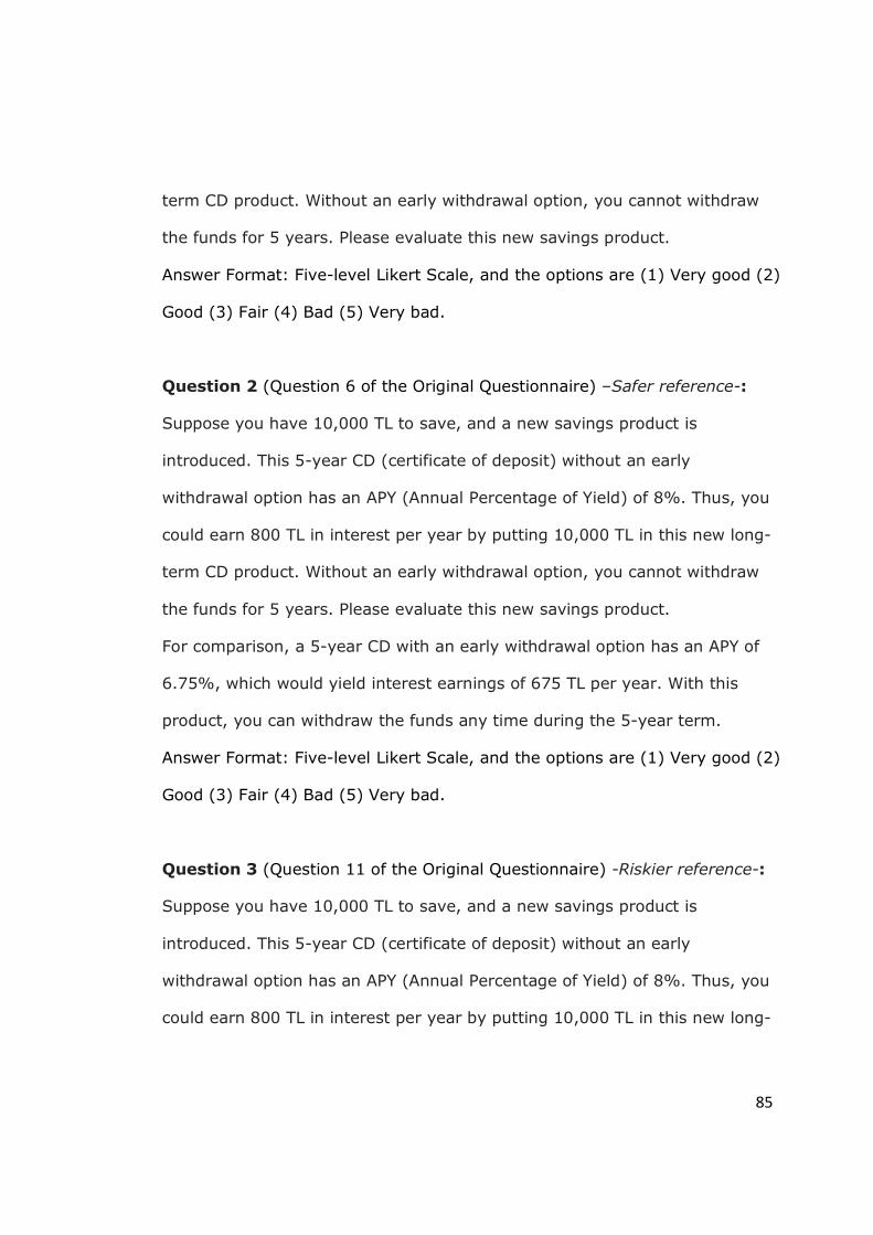
85

term CD product. Without an early withdrawal option, you cannot withdraw

the funds for 5 years. Please evaluate this new savings product.

Answer Format: Five-level Likert Scale, and the options are (1) Very good (2)

Good (3) Fair (4) Bad (5) Very bad.

Question 2 (Question 6 of the Original Questionnaire) –Safer reference-:

Suppose you have 10,000 TL to save, and a new savings product is

introduced. This 5-year CD (certificate of deposit) without an early

withdrawal option has an APY (Annual Percentage of Yield) of 8%. Thus, you

could earn 800 TL in interest per year by putting 10,000 TL in this new long-

term CD product. Without an early withdrawal option, you cannot withdraw

the funds for 5 years. Please evaluate this new savings product.

For comparison, a 5-year CD with an early withdrawal option has an APY of

6.75%, which would yield interest earnings of 675 TL per year. With this

product, you can withdraw the funds any time during the 5-year term.

Answer Format: Five-level Likert Scale, and the options are (1) Very good (2)

Good (3) Fair (4) Bad (5) Very bad.

Question 3 (Question 11 of the Original Questionnaire) -Riskier reference-:

Suppose you have 10,000 TL to save, and a new savings product is

introduced. This 5-year CD (certificate of deposit) without an early

withdrawal option has an APY (Annual Percentage of Yield) of 8%. Thus, you

could earn 800 TL in interest per year by putting 10,000 TL in this new long-

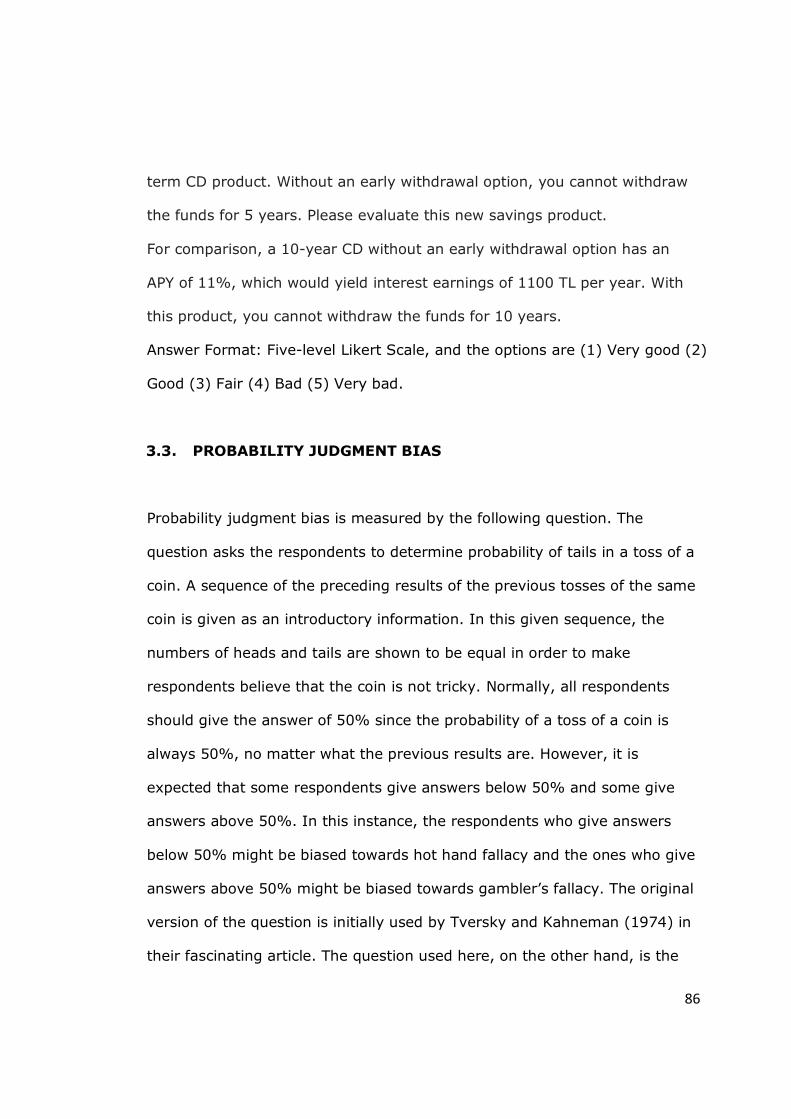
86

term CD product. Without an early withdrawal option, you cannot withdraw

the funds for 5 years. Please evaluate this new savings product.

For comparison, a 10-year CD without an early withdrawal option has an

APY of 11%, which would yield interest earnings of 1100 TL per year. With

this product, you cannot withdraw the funds for 10 years.

Answer Format: Five-level Likert Scale, and the options are (1) Very good (2)

Good (3) Fair (4) Bad (5) Very bad.

3.3. PROBABILITY JUDGMENT BIAS

Probability judgment bias is measured by the following question. The

question asks the respondents to determine probability of tails in a toss of a

coin. A sequence of the preceding results of the previous tosses of the same

coin is given as an introductory information. In this given sequence, the

numbers of heads and tails are shown to be equal in order to make

respondents believe that the coin is not tricky. Normally, all respondents

should give the answer of 50% since the probability of a toss of a coin is

always 50%, no matter what the previous results are. However, it is

expected that some respondents give answers below 50% and some give

answers above 50%. In this instance, the respondents who give answers

below 50% might be biased towards hot hand fallacy and the ones who give

answers above 50% might be biased towards gambler’s fallacy. The original

version of the question is initially used by Tversky and Kahneman (1974) in

their fascinating article. The question used here, on the other hand, is the

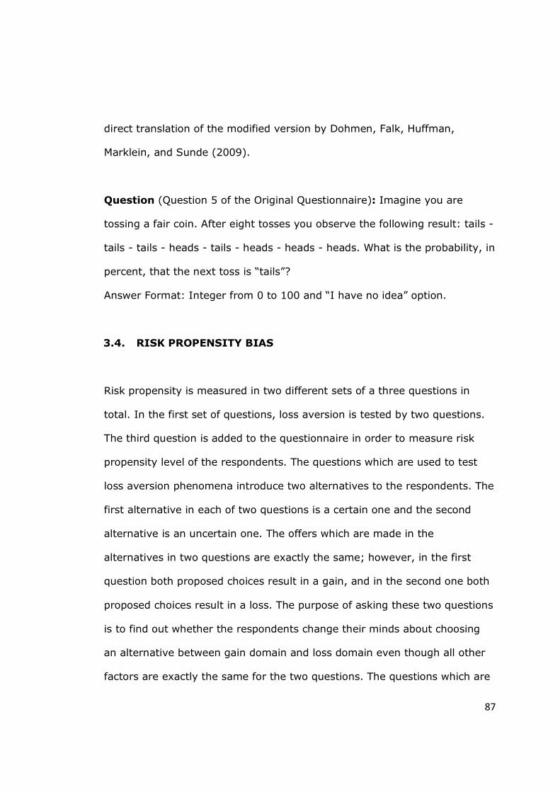
87

direct translation of the modified version by Dohmen, Falk, Huffman,

Marklein, and Sunde (2009).

Question (Question 5 of the Original Questionnaire): Imagine you are

tossing a fair coin. After eight tosses you observe the following result: tails -

tails - tails - heads - tails - heads - heads - heads. What is the probability, in

percent, that the next toss is “tails”?

Answer Format: Integer from 0 to 100 and “I have no idea” option.

3.4. RISK PROPENSITY BIAS

Risk propensity is measured in two different sets of a three questions in

total. In the first set of questions, loss aversion is tested by two questions.

The third question is added to the questionnaire in order to measure risk

propensity level of the respondents. The questions which are used to test

loss aversion phenomena introduce two alternatives to the respondents. The

first alternative in each of two questions is a certain one and the second

alternative is an uncertain one. The offers which are made in the

alternatives in two questions are exactly the same; however, in the first

question both proposed choices result in a gain, and in the second one both

proposed choices result in a loss. The purpose of asking these two questions

is to find out whether the respondents change their minds about choosing

an alternative between gain domain and loss domain even though all other

factors are exactly the same for the two questions. The questions which are

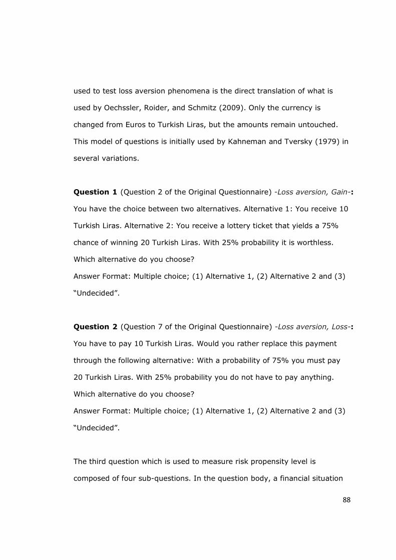
88

used to test loss aversion phenomena is the direct translation of what is

used by Oechssler, Roider, and Schmitz (2009). Only the currency is

changed from Euros to Turkish Liras, but the amounts remain untouched.

This model of questions is initially used by Kahneman and Tversky (1979) in

several variations.

Question 1 (Question 2 of the Original Questionnaire) -Loss aversion, Gain-:

You have the choice between two alternatives. Alternative 1: You receive 10

Turkish Liras. Alternative 2: You receive a lottery ticket that yields a 75%

chance of winning 20 Turkish Liras. With 25% probability it is worthless.

Which alternative do you choose?

Answer Format: Multiple choice; (1) Alternative 1, (2) Alternative 2 and (3)

“Undecided”.

Question 2 (Question 7 of the Original Questionnaire) -Loss aversion, Loss-:

You have to pay 10 Turkish Liras. Would you rather replace this payment

through the following alternative: With a probability of 75% you must pay

20 Turkish Liras. With 25% probability you do not have to pay anything.

Which alternative do you choose?

Answer Format: Multiple choice; (1) Alternative 1, (2) Alternative 2 and (3)

“Undecided”.

The third question which is used to measure risk propensity level is

composed of four sub-questions. In the question body, a financial situation

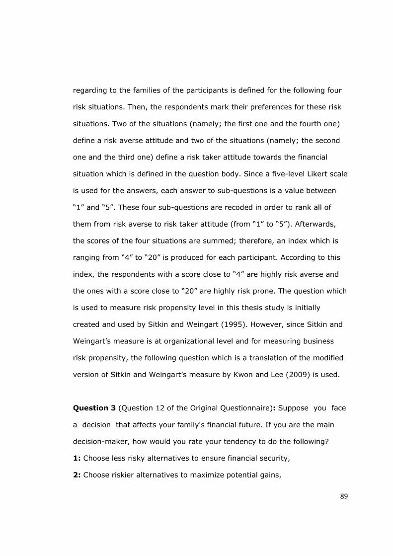
89

regarding to the families of the participants is defined for the following four

risk situations. Then, the respondents mark their preferences for these risk

situations. Two of the situations (namely; the first one and the fourth one)

define a risk averse attitude and two of the situations (namely; the second

one and the third one) define a risk taker attitude towards the financial

situation which is defined in the question body. Since a five-level Likert scale

is used for the answers, each answer to sub-questions is a value between

“1” and “5”. These four sub-questions are recoded in order to rank all of

them from risk averse to risk taker attitude (from “1” to “5”). Afterwards,

the scores of the four situations are summed; therefore, an index which is

ranging from “4” to “20” is produced for each participant. According to this

index, the respondents with a score close to “4” are highly risk averse and

the ones with a score close to “20” are highly risk prone. The question which

is used to measure risk propensity level in this thesis study is initially

created and used by Sitkin and Weingart (1995). However, since Sitkin and

Weingart’s measure is at organizational level and for measuring business

risk propensity, the following question which is a translation of the modified

version of Sitkin and Weingart’s measure by Kwon and Lee (2009) is used.

Question 3 (Question 12 of the Original Questionnaire): Suppose you face

a decision that affects your family's financial future. If you are the main

decision-maker, how would you rate your tendency to do the following?

1: Choose less risky alternatives to ensure financial security,

2: Choose riskier alternatives to maximize potential gains,

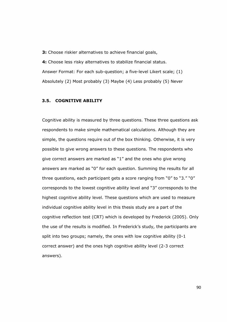
90

3: Choose riskier alternatives to achieve financial goals,

4: Choose less risky alternatives to stabilize financial status.

Answer Format: For each sub-question; a five-level Likert scale; (1)

Absolutely (2) Most probably (3) Maybe (4) Less probably (5) Never

3.5. COGNITIVE ABILITY

Cognitive ability is measured by three questions. These three questions ask

respondents to make simple mathematical calculations. Although they are

simple, the questions require out of the box thinking. Otherwise, it is very

possible to give wrong answers to these questions. The respondents who

give correct answers are marked as “1” and the ones who give wrong

answers are marked as “0” for each question. Summing the results for all

three questions, each participant gets a score ranging from “0” to “3.” “0”

corresponds to the lowest cognitive ability level and “3” corresponds to the

highest cognitive ability level. These questions which are used to measure

individual cognitive ability level in this thesis study are a part of the

cognitive reflection test (CRT) which is developed by Frederick (2005). Only

the use of the results is modified. In Frederick’s study, the participants are

split into two groups; namely, the ones with low cognitive ability (0-1

correct answer) and the ones high cognitive ability level (2-3 correct

answers).

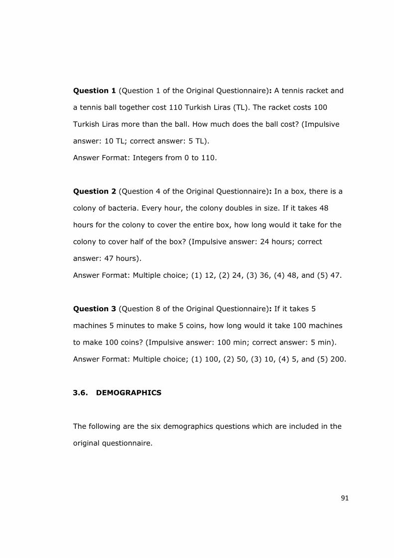
91

Question 1 (Question 1 of the Original Questionnaire): A tennis racket and

a tennis ball together cost 110 Turkish Liras (TL). The racket costs 100

Turkish Liras more than the ball. How much does the ball cost? (Impulsive

answer: 10 TL; correct answer: 5 TL).

Answer Format: Integers from 0 to 110.

Question 2 (Question 4 of the Original Questionnaire): In a box, there is a

colony of bacteria. Every hour, the colony doubles in size. If it takes 48

hours for the colony to cover the entire box, how long would it take for the

colony to cover half of the box? (Impulsive answer: 24 hours; correct

answer: 47 hours).

Answer Format: Multiple choice; (1) 12, (2) 24, (3) 36, (4) 48, and (5) 47.

Question 3 (Question 8 of the Original Questionnaire): If it takes 5

machines 5 minutes to make 5 coins, how long would it take 100 machines

to make 100 coins? (Impulsive answer: 100 min; correct answer: 5 min).

Answer Format: Multiple choice; (1) 100, (2) 50, (3) 10, (4) 5, and (5) 200.

3.6. DEMOGRAPHICS

The following are the six demographics questions which are included in the

original questionnaire.

92

Question 1 (Question 13 of the Original Questionnaire): Age

Answer Format: Integer from 0 to 100.

Question 2 (Question 14 of the Original Questionnaire): Gender

Answer Format: Two choices; (1) Male and (2) Female.

Question 3 (Question 15 of the Original Questionnaire): Please mark your

current and/or completed degrees.

1: Undergraduate Degree

2: Master’s Degree

3: Doctoral Degree

Answer Format: For each question, multiple choice; (1) Educational Sciences,

(2) Arts and Sciences, (3) Fine Arts, (4) Law, (5) Economics and

Administrative Sciences, (6) Architecture, (7) Engineering, (8) Medicine, and

(9) Other Faculty.

Question 4 (Question 16 of the Original Questionnaire): If you are an

undergraduate student, please mark your year of class.

Answer Format: Multiple choice; (1) Prep School, (2) Freshman, (3)

Sophomore, (4) Junior, and (5) Senior.

Question 5 (Question 17 of the Original Questionnaire): What is your

current household income level?

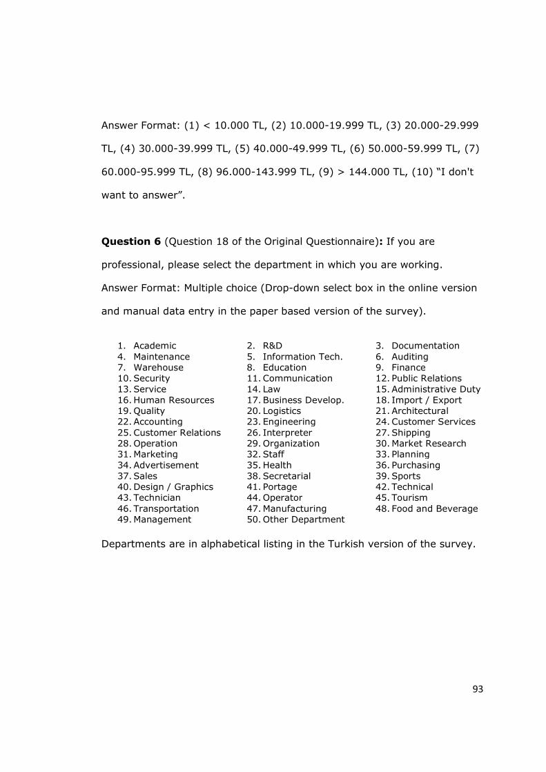
93

Answer Format: (1) < 10.000 TL, (2) 10.000-19.999 TL, (3) 20.000-29.999

TL, (4) 30.000-39.999 TL, (5) 40.000-49.999 TL, (6) 50.000-59.999 TL, (7)

60.000-95.999 TL, (8) 96.000-143.999 TL, (9) > 144.000 TL, (10) “I don't

want to answer”.

Question 6 (Question 18 of the Original Questionnaire): If you are

professional, please select the department in which you are working.

Answer Format: Multiple choice (Drop-down select box in the online version

and manual data entry in the paper based version of the survey).

1. Academic 2. R&D 3. Documentation 4. Maintenance 5. Information Tech. 6. Auditing 7. Warehouse 8. Education 9. Finance 10. Security 11. Communication 12. Public Relations 13. Service 14. Law 15. Administrative Duty 16. Human Resources 17. Business Develop. 18. Import / Export 19. Quality 20. Logistics 21. Architectural 22. Accounting 23. Engineering 24. Customer Services 25. Customer Relations 26. Interpreter 27. Shipping 28. Operation 29. Organization 30. Market Research 31. Marketing 32. Staff 33. Planning 34. Advertisement 35. Health 36. Purchasing 37. Sales 38. Secretarial 39. Sports 40. Design / Graphics 41. Portage 42. Technical 43. Technician 44. Operator 45. Tourism 46. Transportation 47. Manufacturing 48. Food and Beverage 49. Management 50. Other Department

Departments are in alphabetical listing in the Turkish version of the survey.

94

4. SAMPLING AND DATA COLLECTION

The respondents are composed of both professionals and university students.

Working professionals contribute to the online version of the survey and

students fill in mostly paper-based forms. All respondents voluntarily

participate in the survey. Those who contribute to the online version are

asked to do so by sending emails to the alumni lists of Middle East Technical

University and posting calls on social media (Linkedin, Facebook, Twitter,

Blogs etc.). Paper-based surveys, on the other hand, are conducted in class

settings before lectures. Freshman, sophomore, junior, and senior students

of several disciplines are asked to participate in the survey. They are from

Middle East Technical University, TOBB University of Economics and

Technology, Atilim University and Gazi University which are all located in

Ankara, Turkey. The sample is kept as diverse as possible in order to reduce

any possible biases which may be caused by demographics.

In both versions of the survey (online and paper-based), potential

participants are asked to fill in a survey to provide required data for a

master’s thesis study. They are not initially informed about the topic and

about the content of the survey, in order to obtain unbiased testing

environments. It is also important to note that the permission of Middle East

Technical University Ethical Committee is granted before conducting the

survey and the official permission letter is in Appendix VIII.

95

The paper-based version of the survey is in Appendix I and the screenshots

of the online version of the survey are in Appendix III. The paper-based

version is designed in a way to have a compact design; but, since validation

checks are not possible, there are both incomplete questionnaires and

completed questionnaires with invalid answers in the paper-based version.

The online version of the survey, on the other hand, results in only

incomplete questionnaires but not invalid answers. This is because the

online version is coded in a way to validate inputs for each question before

the submission of the survey data. Moreover, in the online version, in order

to reduce the rate of possible incomplete surveys, the survey questions are

distributed into five pages with a better user experience design, encouraging

the respondents to fully complete the survey by providing.

1681 individuals contribute to the survey. 858 of them participate in the

online version, and 823 of them fill in the paper-based version of the survey.

Among 823 respondents, 324 are students from Middle East Technical

University, and the remaining 499 respondents are from the other

universities, mostly from TOBB University of Economics and Technology.

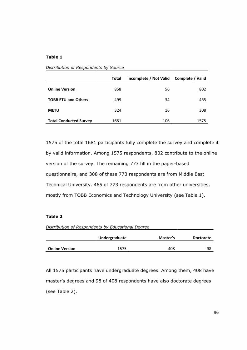
96

Table 1

Distribution of Respondents by Source

Total Incomplete / Not Valid Complete / Valid

Online Version 858 56 802

TOBB ETU and Others 499 34 465

METU 324 16 308

Total Conducted Survey 1681 106 1575

1575 of the total 1681 participants fully complete the survey and complete it

by valid information. Among 1575 respondents, 802 contribute to the online

version of the survey. The remaining 773 fill in the paper-based

questionnaire, and 308 of these 773 respondents are from Middle East

Technical University. 465 of 773 respondents are from other universities,

mostly from TOBB Economics and Technology University (see Table 1).

Table 2

Distribution of Respondents by Educational Degree

Undergraduate Master’s Doctorate

Online Version 1575 408 98

All 1575 participants have undergraduate degrees. Among them, 408 have

master’s degrees and 98 of 408 respondents have also doctorate degrees

(see Table 2).

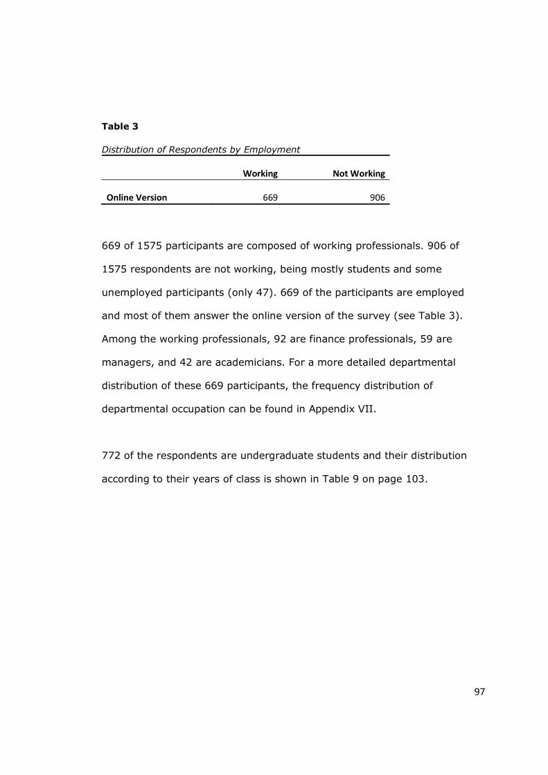
97

Table 3

Distribution of Respondents by Employment

Working Not Working

Online Version 669 906

669 of 1575 participants are composed of working professionals. 906 of

1575 respondents are not working, being mostly students and some

unemployed participants (only 47). 669 of the participants are employed

and most of them answer the online version of the survey (see Table 3).

Among the working professionals, 92 are finance professionals, 59 are

managers, and 42 are academicians. For a more detailed departmental

distribution of these 669 participants, the frequency distribution of

departmental occupation can be found in Appendix VII.

772 of the respondents are undergraduate students and their distribution

according to their years of class is shown in Table 9 on page 103.

98

5. ANALYSES AND RESULTS

The data are analyzed by the statistical software package SPSS version 16.

In order the analyses to be followed clearly, the coded version of the

questionnaire is available in Appendix II (in Turkish).

On the following pages, the descriptive statistics for the answers of each

survey question are presented. Next, the hypotheses are restated, the tests

for each hypothesis are conducted, and the corresponding results are

demonstrated. Last but not least, regression analyses of statistically

significant biases are run to examine the effects of individual cognitive

ability levels and some demographic variables on those biases.

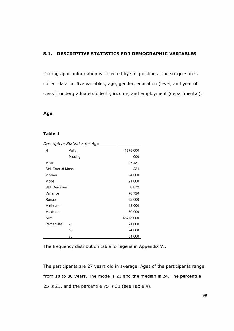
99

5.1. DESCRIPTIVE STATISTICS FOR DEMOGRAPHIC VARIABLES

Demographic information is collected by six questions. The six questions

collect data for five variables; age, gender, education (level, and year of

class if undergraduate student), income, and employment (departmental).

Age

Table 4

Descriptive Statistics for Age

N Valid 1575,000

Missing ,000

Mean 27,437

Std. Error of Mean ,224

Median 24,000

Mode 21,000

Std. Deviation 8,872

Variance 78,720

Range 62,000

Minimum 18,000

Maximum 80,000

Sum 43213,000

Percentiles 25 21,000

50 24,000

75 31,000

The frequency distribution table for age is in Appendix VI.

The participants are 27 years old in average. Ages of the participants range

from 18 to 80 years. The mode is 21 and the median is 24. The percentile

25 is 21, and the percentile 75 is 31 (see Table 4).

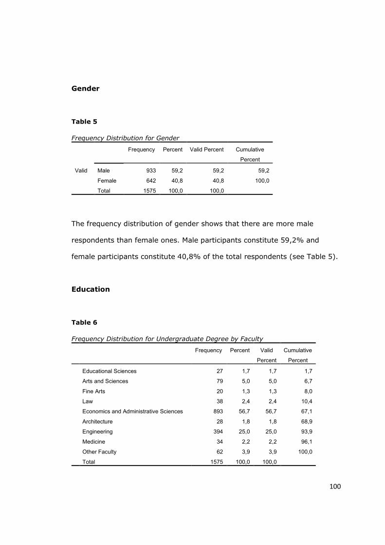
100

Gender

Table 5

Frequency Distribution for Gender

Frequency Percent Valid Percent Cumulative

Percent

Valid Male 933 59,2 59,2 59,2

Female 642 40,8 40,8 100,0

Total 1575 100,0 100,0

The frequency distribution of gender shows that there are more male

respondents than female ones. Male participants constitute 59,2% and

female participants constitute 40,8% of the total respondents (see Table 5).

Education

Table 6

Frequency Distribution for Undergraduate Degree by Faculty Frequency Percent Valid

Percent

Cumulative

Percent

Educational Sciences 27 1,7 1,7 1,7

Arts and Sciences 79 5,0 5,0 6,7

Fine Arts 20 1,3 1,3 8,0

Law 38 2,4 2,4 10,4

Economics and Administrative Sciences 893 56,7 56,7 67,1

Architecture 28 1,8 1,8 68,9

Engineering 394 25,0 25,0 93,9

Medicine 34 2,2 2,2 96,1

Other Faculty 62 3,9 3,9 100,0

Total 1575 100,0 100,0

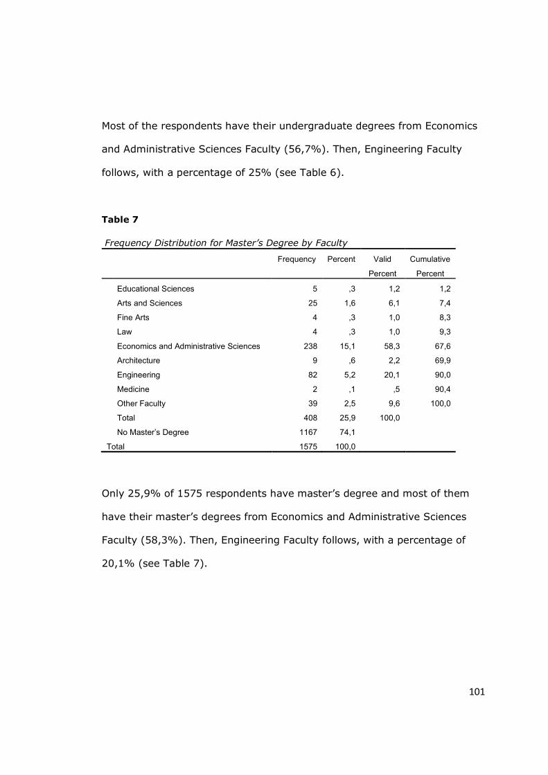
101

Most of the respondents have their undergraduate degrees from Economics

and Administrative Sciences Faculty (56,7%). Then, Engineering Faculty

follows, with a percentage of 25% (see Table 6).

Table 7

Frequency Distribution for Master’s Degree by Faculty

Frequency Percent Valid

Percent

Cumulative

Percent

Educational Sciences 5 ,3 1,2 1,2

Arts and Sciences 25 1,6 6,1 7,4

Fine Arts 4 ,3 1,0 8,3

Law 4 ,3 1,0 9,3

Economics and Administrative Sciences 238 15,1 58,3 67,6

Architecture 9 ,6 2,2 69,9

Engineering 82 5,2 20,1 90,0

Medicine 2 ,1 ,5 90,4

Other Faculty 39 2,5 9,6 100,0

Total 408 25,9 100,0

No Master’s Degree 1167 74,1

Total 1575 100,0

Only 25,9% of 1575 respondents have master’s degree and most of them

have their master’s degrees from Economics and Administrative Sciences

Faculty (58,3%). Then, Engineering Faculty follows, with a percentage of

20,1% (see Table 7).

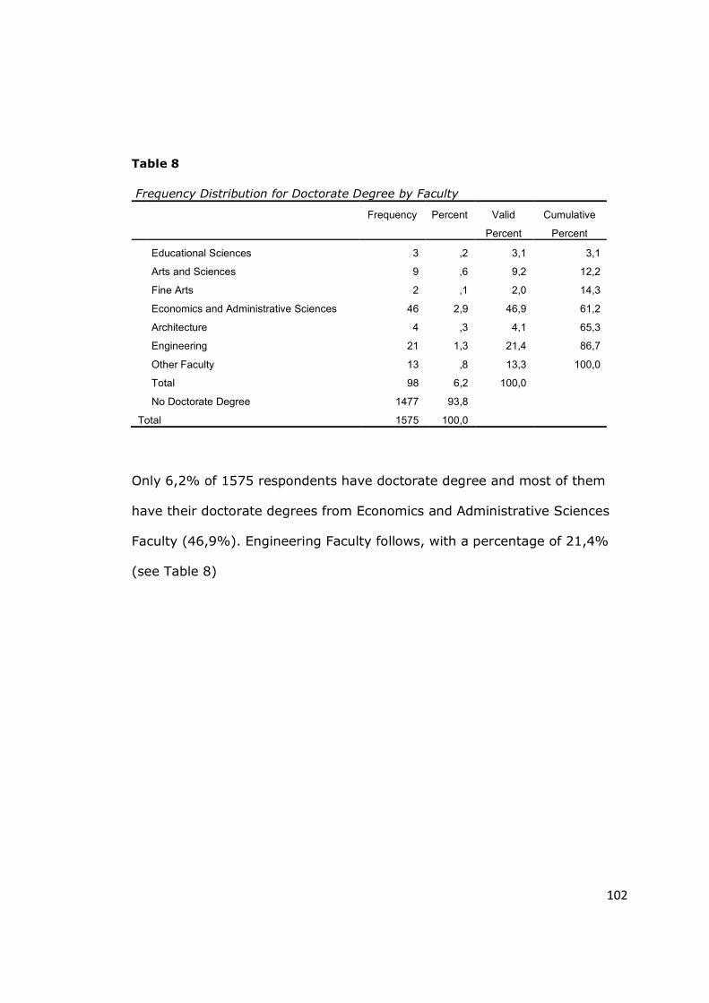
102

Table 8

Frequency Distribution for Doctorate Degree by Faculty Frequency Percent Valid

Percent

Cumulative

Percent

Educational Sciences 3 ,2 3,1 3,1

Arts and Sciences 9 ,6 9,2 12,2

Fine Arts 2 ,1 2,0 14,3

Economics and Administrative Sciences 46 2,9 46,9 61,2

Architecture 4 ,3 4,1 65,3

Engineering 21 1,3 21,4 86,7

Other Faculty 13 ,8 13,3 100,0

Total 98 6,2 100,0

No Doctorate Degree 1477 93,8

Total 1575 100,0

Only 6,2% of 1575 respondents have doctorate degree and most of them

have their doctorate degrees from Economics and Administrative Sciences

Faculty (46,9%). Engineering Faculty follows, with a percentage of 21,4%

(see Table 8)

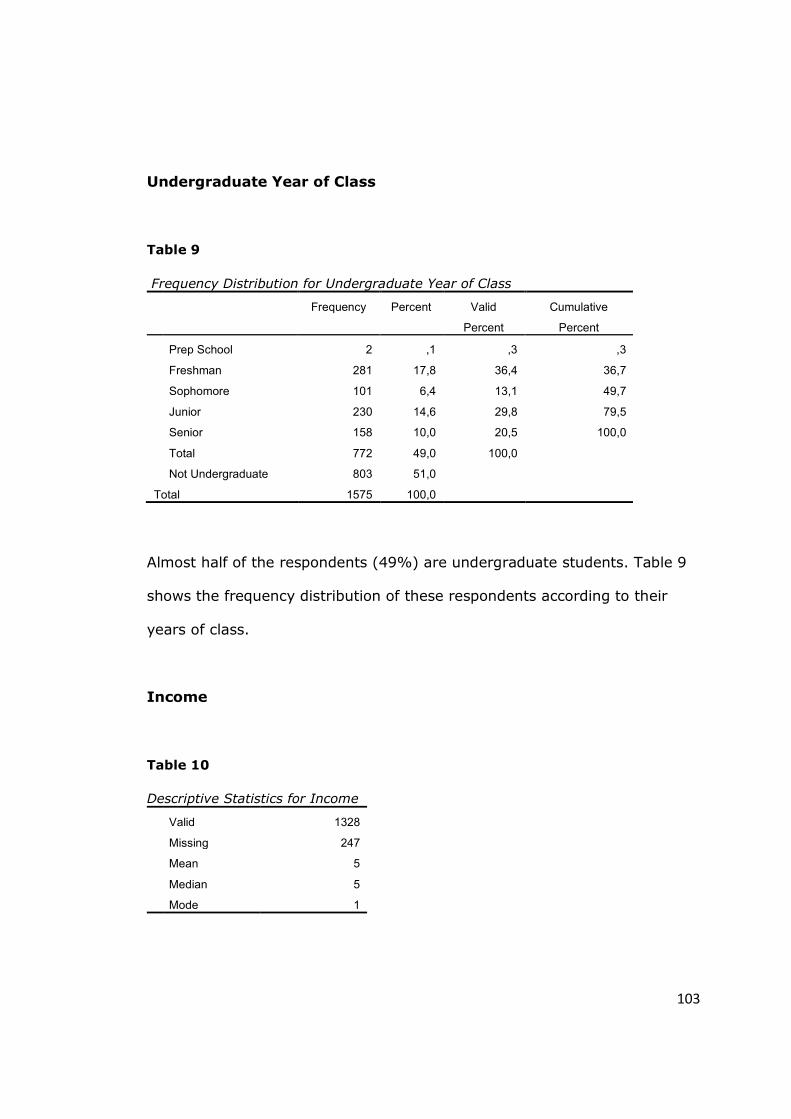
103

Undergraduate Year of Class

Table 9

Frequency Distribution for Undergraduate Year of Class

Frequency Percent Valid

Percent

Cumulative

Percent

Prep School 2 ,1 ,3 ,3

Freshman 281 17,8 36,4 36,7

Sophomore 101 6,4 13,1 49,7

Junior 230 14,6 29,8 79,5

Senior 158 10,0 20,5 100,0

Total 772 49,0 100,0

Not Undergraduate 803 51,0

Total 1575 100,0

Almost half of the respondents (49%) are undergraduate students. Table 9

shows the frequency distribution of these respondents according to their

years of class.

Income

Table 10

Descriptive Statistics for Income

Valid 1328

Missing 247

Mean 5

Median 5

Mode 1

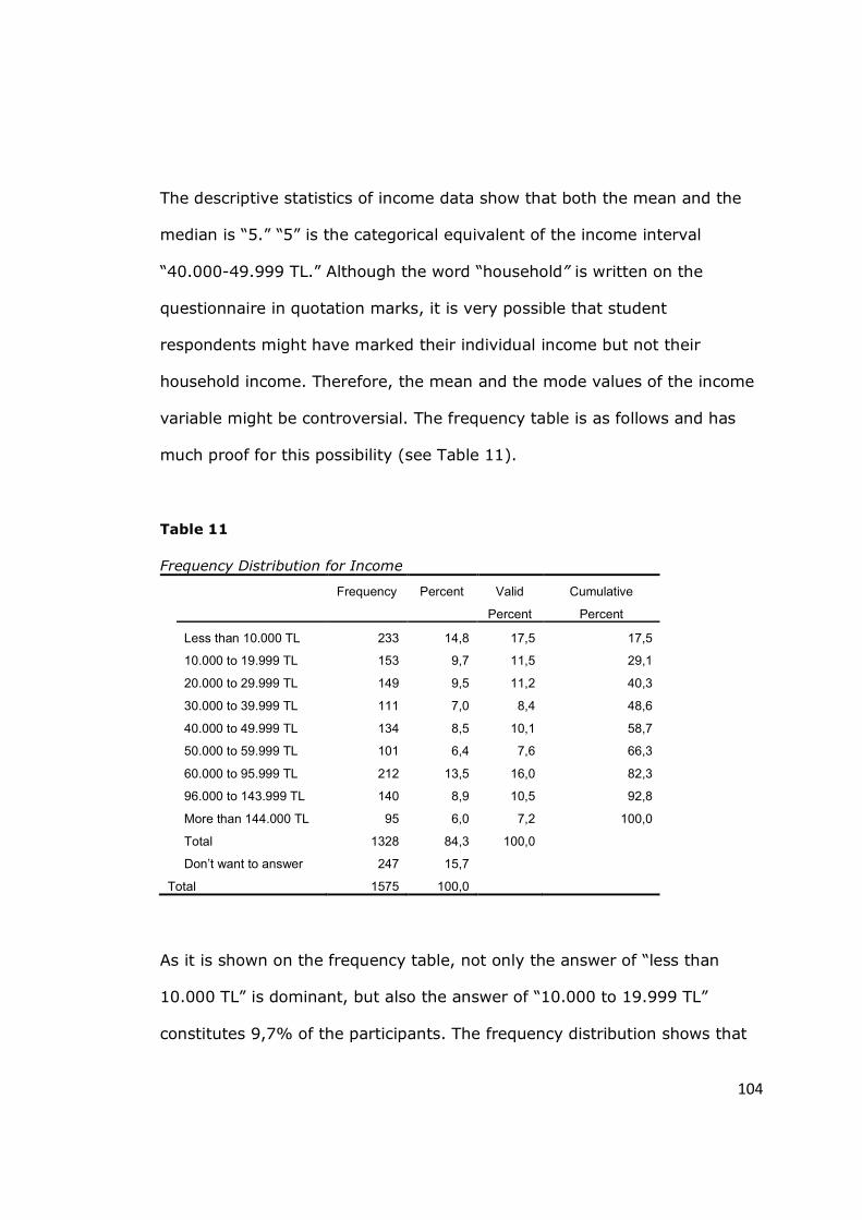
104

The descriptive statistics of income data show that both the mean and the

median is “5.” “5” is the categorical equivalent of the income interval

“40.000-49.999 TL.” Although the word “household” is written on the

questionnaire in quotation marks, it is very possible that student

respondents might have marked their individual income but not their

household income. Therefore, the mean and the mode values of the income

variable might be controversial. The frequency table is as follows and has

much proof for this possibility (see Table 11).

Table 11

Frequency Distribution for Income

Frequency Percent Valid

Percent

Cumulative

Percent

Less than 10.000 TL 233 14,8 17,5 17,5

10.000 to 19.999 TL 153 9,7 11,5 29,1

20.000 to 29.999 TL 149 9,5 11,2 40,3

30.000 to 39.999 TL 111 7,0 8,4 48,6

40.000 to 49.999 TL 134 8,5 10,1 58,7

50.000 to 59.999 TL 101 6,4 7,6 66,3

60.000 to 95.999 TL 212 13,5 16,0 82,3

96.000 to 143.999 TL 140 8,9 10,5 92,8

More than 144.000 TL 95 6,0 7,2 100,0

Total 1328 84,3 100,0

Don’t want to answer 247 15,7

Total 1575 100,0

As it is shown on the frequency table, not only the answer of “less than

10.000 TL” is dominant, but also the answer of “10.000 to 19.999 TL”

constitutes 9,7% of the participants. The frequency distribution shows that

105

24,5% of all participants have a household income 19.999 TL or lower. The

highest percentage following the first one is 13,5% which corresponds to the

“60.000 to 95.999 TL” interval (See Table 11).

Occupation

1. Academic 2. R&D 3. Documentation 4. Maintenance 5. Information Tech. 6. Auditing 7. Warehouse 8. Education 9. Finance 10. Security 11. Communication 12. Public Relations 13. Service 14. Law 15. Administrative Duty 16. Human Resources 17. Business Develop. 18. Import / Export 19. Quality 20. Logistics 21. Architectural 22. Accounting 23. Engineering 24. Customer Services 25. Customer Relations 26. Interpreter 27. Shipping 28. Operation 29. Organization 30. Market Research 31. Marketing 32. Staff 33. Planning 34. Advertisement 35. Health 36. Purchasing 37. Sales 38. Secretarial 39. Sports 40. Design / Graphics 41. Portage 42. Technical 43. Technician 44. Operator 45. Tourism 46. Transportation 47. Manufacturing 48. Food and Beverage 49. Management 50. Other Department

The frequency distribution table for the occupation is in Appendix VII.

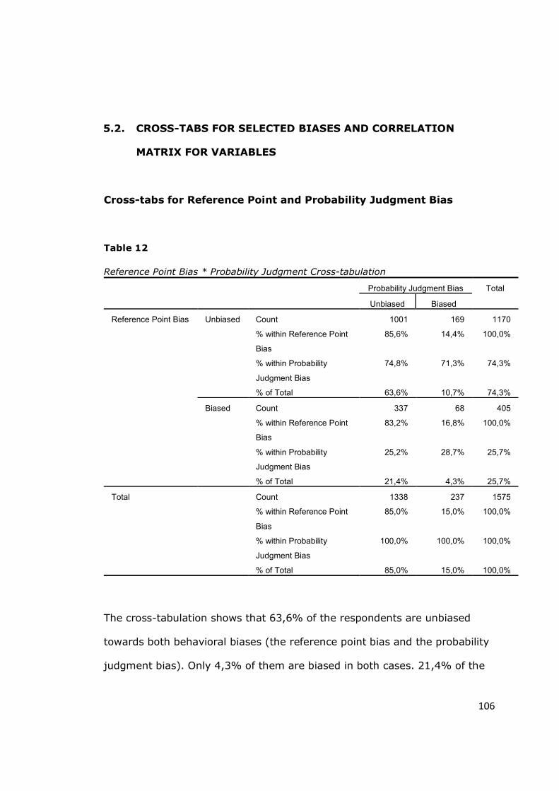
106

5.2. CROSS-TABS FOR SELECTED BIASES AND CORRELATION

MATRIX FOR VARIABLES

Cross-tabs for Reference Point and Probability Judgment Bias

Table 12

Reference Point Bias * Probability Judgment Cross-tabulation

Probability Judgment Bias Total

Unbiased Biased

Reference Point Bias Unbiased Count 1001 169 1170

% within Reference Point

Bias

85,6% 14,4% 100,0%

% within Probability

Judgment Bias

74,8% 71,3% 74,3%

% of Total 63,6% 10,7% 74,3%

Biased Count 337 68 405

% within Reference Point

Bias

83,2% 16,8% 100,0%

% within Probability

Judgment Bias

25,2% 28,7% 25,7%

% of Total 21,4% 4,3% 25,7%

Total Count 1338 237 1575

% within Reference Point

Bias

85,0% 15,0% 100,0%

% within Probability

Judgment Bias

100,0% 100,0% 100,0%

% of Total 85,0% 15,0% 100,0%

The cross-tabulation shows that 63,6% of the respondents are unbiased

towards both behavioral biases (the reference point bias and the probability

judgment bias). Only 4,3% of them are biased in both cases. 21,4% of the

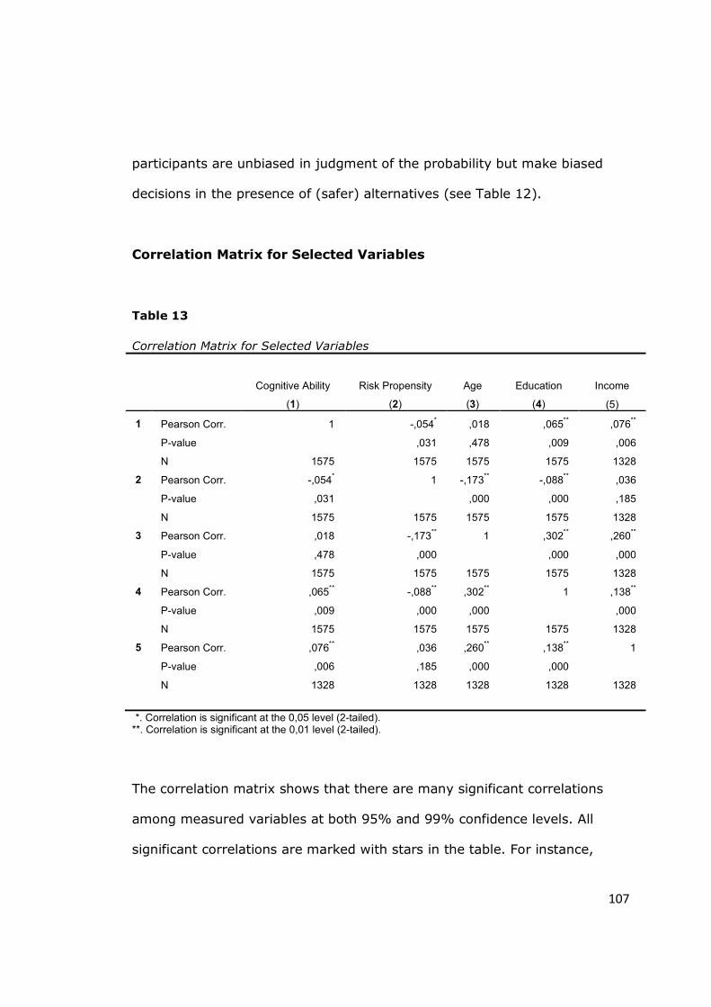
107

participants are unbiased in judgment of the probability but make biased

decisions in the presence of (safer) alternatives (see Table 12).

Correlation Matrix for Selected Variables

Table 13

Correlation Matrix for Selected Variables

Cognitive Ability

(1)

Risk Propensity

(2)

Age

(3)

Education

(4)

Income

(5)

1 Pearson Corr. 1 -,054* ,018 ,065

** ,076

**

P-value ,031 ,478 ,009 ,006

N 1575 1575 1575 1575 1328

2 Pearson Corr. -,054* 1 -,173

** -,088

** ,036

P-value ,031 ,000 ,000 ,185

N 1575 1575 1575 1575 1328

3 Pearson Corr. ,018 -,173** 1 ,302

** ,260

**

P-value ,478 ,000 ,000 ,000

N 1575 1575 1575 1575 1328

4 Pearson Corr. ,065** -,088

** ,302

** 1 ,138

**

P-value ,009 ,000 ,000 ,000

N 1575 1575 1575 1575 1328

5 Pearson Corr. ,076** ,036 ,260

** ,138

** 1

P-value ,006 ,185 ,000 ,000

N 1328 1328 1328 1328 1328

*. Correlation is significant at the 0,05 level (2-tailed). **. Correlation is significant at the 0,01 level (2-tailed).

The correlation matrix shows that there are many significant correlations

among measured variables at both 95% and 99% confidence levels. All

significant correlations are marked with stars in the table. For instance,

108

cognitive ability is found to be negatively correlated with risk propensity with

a correlation coefficient of -0,054 (p-value is 0,031). It is also shown that

cognitive ability is in positive correlation with education at the 0,01 level, as

it is with income. Cognitive ability is not correlated with age at a statistically

significant level. Risk propensity is, on the other hand, negatively correlated

with age (coefficient is -0,082 and p-value is 0,000), and education

(coefficient is -0,088 and p-value is 0,000). It is shown that risk propensity

is not significantly correlated with income. For all significant correlations,

please see Table 13.

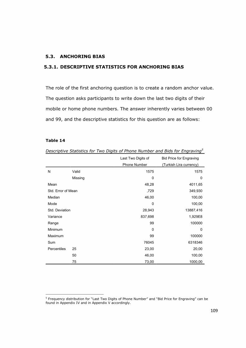
109

5.3. ANCHORING BIAS

5.3.1. DESCRIPTIVE STATISTICS FOR ANCHORING BIAS

The role of the first anchoring question is to create a random anchor value.

The question asks participants to write down the last two digits of their

mobile or home phone numbers. The answer inherently varies between 00

and 99, and the descriptive statistics for this question are as follows:

Table 14

Descriptive Statistics for Two Digits of Phone Number and Bids for Engraving5

Last Two Digits of

Phone Number

Bid Price for Engraving

(Turkish Lira currency)

N Valid 1575 1575

Missing 0 0

Mean 48,28 4011,65

Std. Error of Mean ,729 349,930

Median 46,00 100,00

Mode 0 100,00

Std. Deviation 28,943 13887,416

Variance 837,698 1,929E8

Range 99 100000

Minimum 0 0

Maximum 99 100000

Sum 76045 6318346

Percentiles 25 23,00 20,00

50 46,00 100,00

75 73,00 1000,00

5 Frequency distribution for “Last Two Digits of Phone Number” and “Bid Price for Engraving” can be found in Appendix IV and in Appendix V accordingly.

110

The descriptive statistics of the answers to the first anchoring question

(Table 14) show that the mean is 48,28 and the median is 46,00. These are

very close to the ideal mean and the median of 49,50 as if there should be

one of each number from 00 to 99 in a 100-values distribution. The

frequency table of the data can be found in Appendix IV.

The second question which measures anchoring bias asks the participants to

make an offer for a copy of the engraving which is defined in the question in

detail. The results are ranging from 0 to 100.000 TL and the descriptive

statistics are as shown on the previous page. The mode and the median of

the data is 100 TL. The mean of all the bids is 4011,65 TL. The frequency

table for the bids on the engraving can be found in Appendix V.

5.3.2. HYPOTHESES ON ANCHORING BIAS

Hypothesis 1

H10: The participants with higher last two digits of phone numbers will not

tend to bid higher amounts for the focal product (the engraving).

H11: The participants with higher last two digits of phone numbers will tend

to bid higher amounts for the focal product (the engraving).

The role of the first anchoring question is to create a random anchor value

which is not compared to the value of the focal product, and it is random,

uninformative, and irrelevant. The question asks participants to write down

111

the last two digits of their mobile or home phone numbers. The answer

inherently varies between “00” and “99”.

The second anchoring question asks the participants to make an offer for a

copy of the engraving which is defined in the question in detail. Hypothesis 1

tests whether the two digits which are written down as an answer to the first

question affect the answers given to the second question. The answers

which are given to the second question are ranging from 0 TL to 100.000 TL.

To test whether Hypothesis 1 is supported or not, a correlation between the

answers to the first question and the answers to the second question is

required to be inspected. The results of the Pearson correlation for these two

data sets are as follows.

Table 15

Correlation between Two Digits of Phone Number (Anchor Value) and Bids for

Engraving (Focal Product)

Anchor Value Bids for Engraving

Anchor Value Pearson Correlation 1,000 ,001

P-value ,954

N 1575,000 1575

Bids for Engraving Pearson Correlation ,001 1,000

P-value ,954

N 1575 1575,000

As seen on Table 15, the Pearson correlation coefficient is found to be 0,001

(p-value is 0,954) meaning that there is not a statistically significant

112

correlation between the anchor values (the last two digits of phone numbers)

and the prices which are offered for the engraving. Ariely, Loewenstein, and

Prelec (2003) ask the subjects of their experiment to compare arbitrary

anchors with the value of the focal product before asking them to evaluate it.

They find a significant anchoring effect. On the other hand, Wilson, Houston,

Etling, and Brekke (1996) do not ask the participants of their study to relate

the anchors to the focal product. However, they also find a significant

anchoring effect. In brief, both Ariely, Loewenstein, and Prelec and Wilson,

Houston, Etling, and Brekke find a significant anchoring effect even though

their methods are different, the latter measuring the basic anchoring effect

as it is measured also in this thesis study. Therefore, it is clear that the

results are contradictory to previous researches in which the anchor values

are found to have a significant effect on different kind of decisions although

they use various methods (see Tversky and Kahneman, 1974; Cervone and

Peake, 1986; Johnson and Schkade, 1989; Jacowitz and Kahneman, 1995;

Wilson, Houston, Etling, and Brekke, 1996; Mussweiler and Strack, 1999;

Chapman and Johnson, 1999; Ariely, Loewenstein, and Prelec, 2003;

Oechssler, Roider, and Schmitz, 2009; and Kudryavtsev and Cohen, 2010).

The reason why the null hypothesis is failed to be rejected may be the

complexity of the focal product under evaluation. It is possible that the

participants might not have understood what the focal product really is since

engraving is not popular anymore. This may also explain the wide range of

the answers from 0 TL to 100.000 TL. Another possible reason might be the

length of the questionnaire and the corresponding fact that there are several

113

digits on the previous questions of the survey. This complexity might have

prevented the effect of the randomly created anchor values. In any case, no

relationship between the uninformative, irrelevant anchor values and the

evaluation of the focal product (engraving) is found; therefore, there is a

statistically significant evidence that the participants with higher last two

digits of phone numbers will not tend to bid higher amounts for the focal

product (the engraving). The null hypothesis is failed to be rejected; thus,

there is not sufficient evidence to support the alternative hypotheses.

5.4. REFERENCE POINT BIAS

5.4.1. DESCRIPTIVE STATISTICS FOR REFERENCE POINT BIAS

The respondents are asked to evaluate a new financial product (a certificate

of deposit) initially alone (base scenario), later together with a safer

reference point, and after that with a riskier reference point.

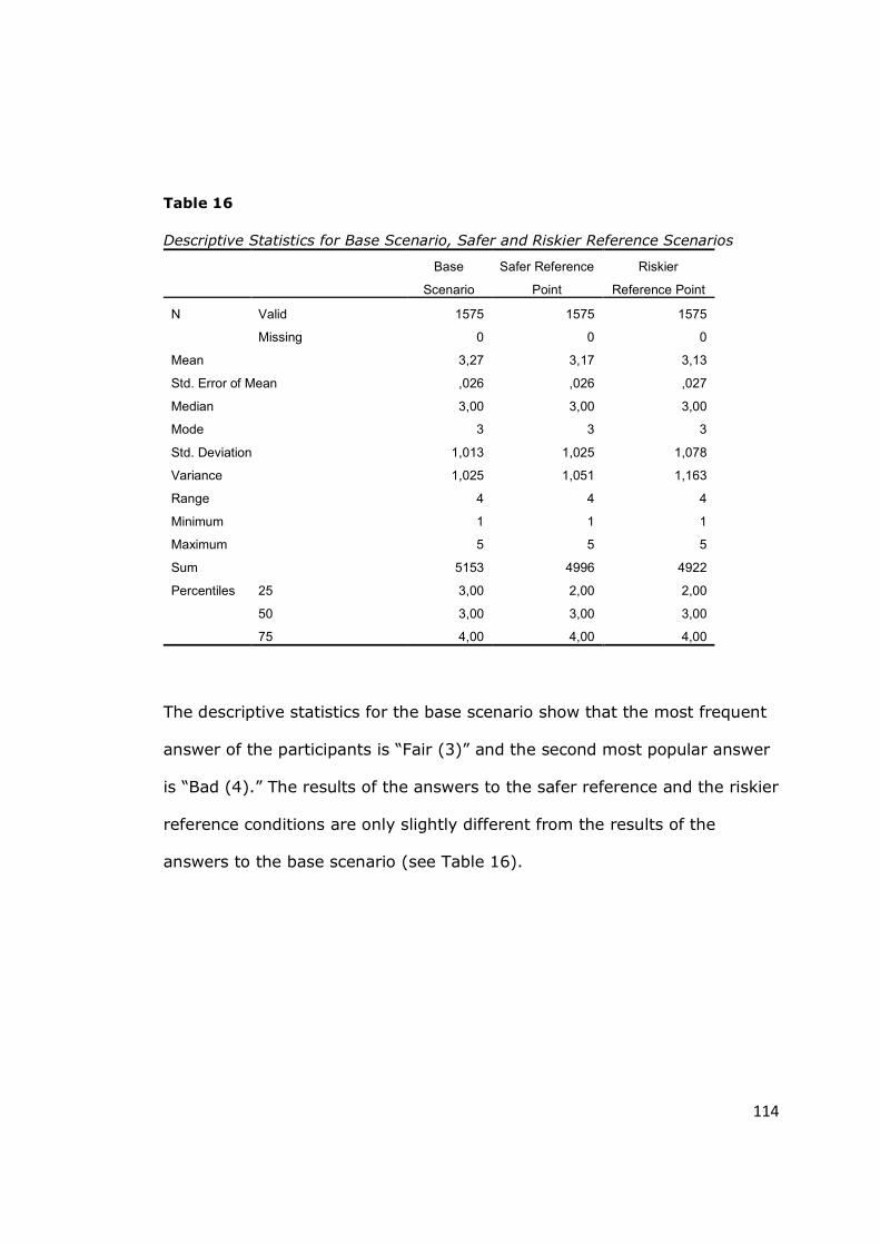
114

Table 16

Descriptive Statistics for Base Scenario, Safer and Riskier Reference Scenarios

Base

Scenario

Safer Reference

Point

Riskier

Reference Point

N Valid 1575 1575 1575

Missing 0 0 0

Mean 3,27 3,17 3,13

Std. Error of Mean ,026 ,026 ,027

Median 3,00 3,00 3,00

Mode 3 3 3

Std. Deviation 1,013 1,025 1,078

Variance 1,025 1,051 1,163

Range 4 4 4

Minimum 1 1 1

Maximum 5 5 5

Sum 5153 4996 4922

Percentiles 25 3,00 2,00 2,00

50 3,00 3,00 3,00

75 4,00 4,00 4,00

The descriptive statistics for the base scenario show that the most frequent

answer of the participants is “Fair (3)” and the second most popular answer

is “Bad (4).” The results of the answers to the safer reference and the riskier

reference conditions are only slightly different from the results of the

answers to the base scenario (see Table 16).

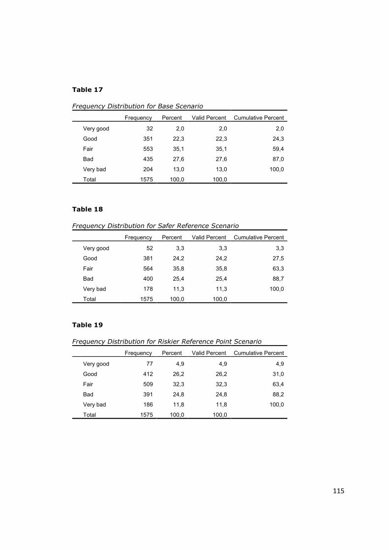
115

Table 17

Frequency Distribution for Base Scenario

Frequency Percent Valid Percent Cumulative Percent

Very good 32 2,0 2,0 2,0

Good 351 22,3 22,3 24,3

Fair 553 35,1 35,1 59,4

Bad 435 27,6 27,6 87,0

Very bad 204 13,0 13,0 100,0

Total 1575 100,0 100,0

Table 18

Frequency Distribution for Safer Reference Scenario

Frequency Percent Valid Percent Cumulative Percent

Very good 52 3,3 3,3 3,3

Good 381 24,2 24,2 27,5

Fair 564 35,8 35,8 63,3

Bad 400 25,4 25,4 88,7

Very bad 178 11,3 11,3 100,0

Total 1575 100,0 100,0

Table 19

Frequency Distribution for Riskier Reference Point Scenario

Frequency Percent Valid Percent Cumulative Percent

Very good 77 4,9 4,9 4,9

Good 412 26,2 26,2 31,0

Fair 509 32,3 32,3 63,4

Bad 391 24,8 24,8 88,2

Very bad 186 11,8 11,8 100,0

Total 1575 100,0 100,0

116

According to the frequency distributions (Table 17, 18 and 19), “Fair” is the

most frequent answer in all three conditions. “Good” and “Bad” follow it. The

frequency distributions show that the results are only slightly different from

each other. This might be the expected result since the focal product under

evaluation is the same for all three conditions.

5.4.2. HYPOTHESES ON REFERENCE POINT BIAS

Hypothesis 2

H20: In the evaluation of a financial product, providing a safer (and lower

return) reference will not make the focal product more attractive.

H21: In the evaluation of a financial product, providing a safer (and lower

return) reference will make the focal product more attractive.

The hypothesis tests whether the same participants evaluate the focal

product in the base scenario condition different from the safer reference

point condition in which there is also a relatively safer alternative to the

focal product, unlike the base scenario in which the focal product is

presented alone.

According to Hypothesis 2, if the participants perceive the same product

more attractive when there is a safer reference point, then the answers to

the safer reference condition should be at least a level more positive than

the answers to the base scenario condition for the same respondents.

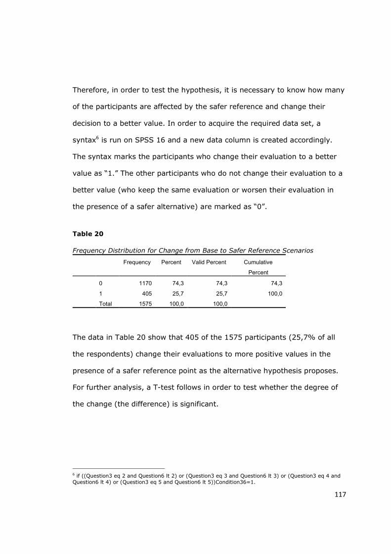
117

Therefore, in order to test the hypothesis, it is necessary to know how many

of the participants are affected by the safer reference and change their

decision to a better value. In order to acquire the required data set, a

syntax6 is run on SPSS 16 and a new data column is created accordingly.

The syntax marks the participants who change their evaluation to a better

value as “1.” The other participants who do not change their evaluation to a

better value (who keep the same evaluation or worsen their evaluation in

the presence of a safer alternative) are marked as “0”.

Table 20

Frequency Distribution for Change from Base to Safer Reference Scenarios

Frequency Percent Valid Percent Cumulative

Percent

0 1170 74,3 74,3 74,3

1 405 25,7 25,7 100,0

Total 1575 100,0 100,0

The data in Table 20 show that 405 of the 1575 participants (25,7% of all

the respondents) change their evaluations to more positive values in the

presence of a safer reference point as the alternative hypothesis proposes.

For further analysis, a T-test follows in order to test whether the degree of

the change (the difference) is significant.

6 if ((Question3 eq 2 and Question6 lt 2) or (Question3 eq 3 and Question6 lt 3) or (Question3 eq 4 and Question6 lt 4) or (Question3 eq 5 and Question6 lt 5))Condition36=1.

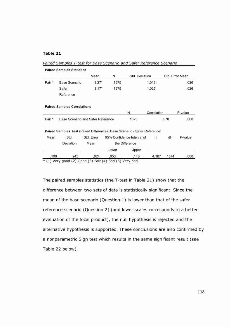
118

Table 21

Paired Samples T-test for Base Scenario and Safer Reference Scenario

Paired Samples Statistics

Mean N Std. Deviation Std. Error Mean

Pair 1 Base Scenario 3,27* 1575 1,013 ,026

Safer

Reference

3,17* 1575 1,025 ,026

Paired Samples Correlations

N Correlation P-value

Pair 1 Base Scenario and Safer Reference 1575 ,570 ,000

Paired Samples Test (Paired Differences: Base Scenario - Safer Reference)

Mean Std.

Deviation

Std. Error

Mean

95% Confidence Interval of

the Difference

t df P-value

Lower Upper

,100 ,945 ,024 ,053 ,146 4,187 1574 ,000

* (1) Very good (2) Good (3) Fair (4) Bad (5) Very bad.

The paired samples statistics (the T-test in Table 21) show that the

difference between two sets of data is statistically significant. Since the

mean of the base scenario (Question 1) is lower than that of the safer

reference scenario (Question 2) (and lower scales corresponds to a better

evaluation of the focal product), the null hypothesis is rejected and the

alternative hypothesis is supported. These conclusions are also confirmed by

a nonparametric Sign test which results in the same significant result (see

Table 22 below).

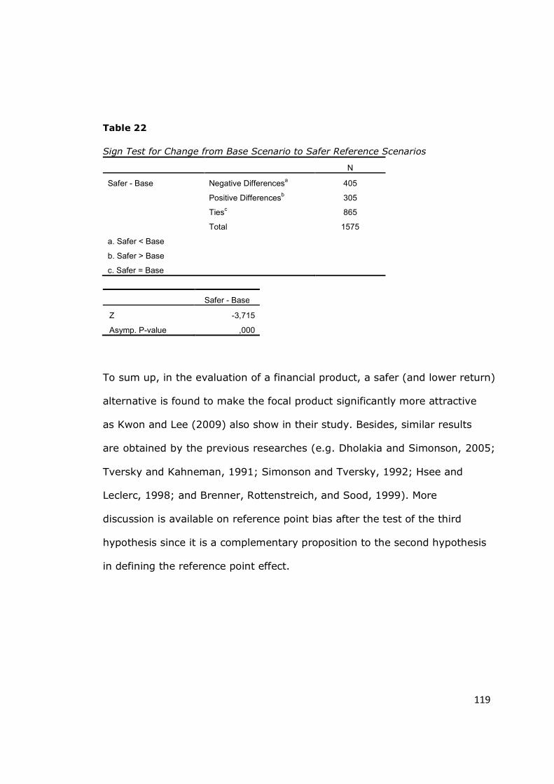
119

Table 22

Sign Test for Change from Base Scenario to Safer Reference Scenarios

N

Safer - Base Negative Differencesa 405

Positive Differencesb 305

Tiesc 865

Total 1575

a. Safer < Base

b. Safer > Base

c. Safer = Base

Safer - Base

Z -3,715

Asymp. P-value ,000

To sum up, in the evaluation of a financial product, a safer (and lower return)

alternative is found to make the focal product significantly more attractive

as Kwon and Lee (2009) also show in their study. Besides, similar results

are obtained by the previous researches (e.g. Dholakia and Simonson, 2005;

Tversky and Kahneman, 1991; Simonson and Tversky, 1992; Hsee and

Leclerc, 1998; and Brenner, Rottenstreich, and Sood, 1999). More

discussion is available on reference point bias after the test of the third

hypothesis since it is a complementary proposition to the second hypothesis

in defining the reference point effect.

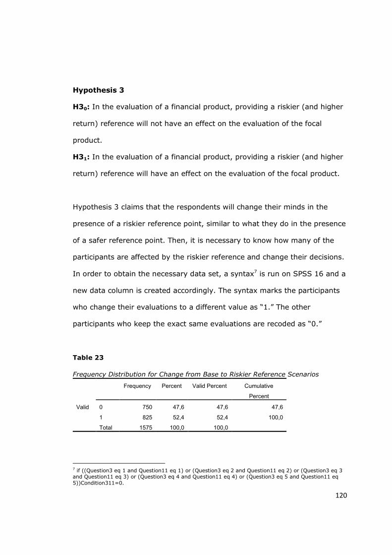
120

Hypothesis 3

H30: In the evaluation of a financial product, providing a riskier (and higher

return) reference will not have an effect on the evaluation of the focal

product.

H31: In the evaluation of a financial product, providing a riskier (and higher

return) reference will have an effect on the evaluation of the focal product.

Hypothesis 3 claims that the respondents will change their minds in the

presence of a riskier reference point, similar to what they do in the presence

of a safer reference point. Then, it is necessary to know how many of the

participants are affected by the riskier reference and change their decisions.

In order to obtain the necessary data set, a syntax7 is run on SPSS 16 and a

new data column is created accordingly. The syntax marks the participants

who change their evaluations to a different value as “1.” The other

participants who keep the exact same evaluations are recoded as “0.”

Table 23

Frequency Distribution for Change from Base to Riskier Reference Scenarios

Frequency Percent Valid Percent Cumulative

Percent

Valid 0 750 47,6 47,6 47,6

1 825 52,4 52,4 100,0

Total 1575 100,0 100,0

7 if ((Question3 eq 1 and Question11 eq 1) or (Question3 eq 2 and Question11 eq 2) or (Question3 eq 3 and Question11 eq 3) or (Question3 eq 4 and Question11 eq 4) or (Question3 eq 5 and Question11 eq 5))Condition311=0.

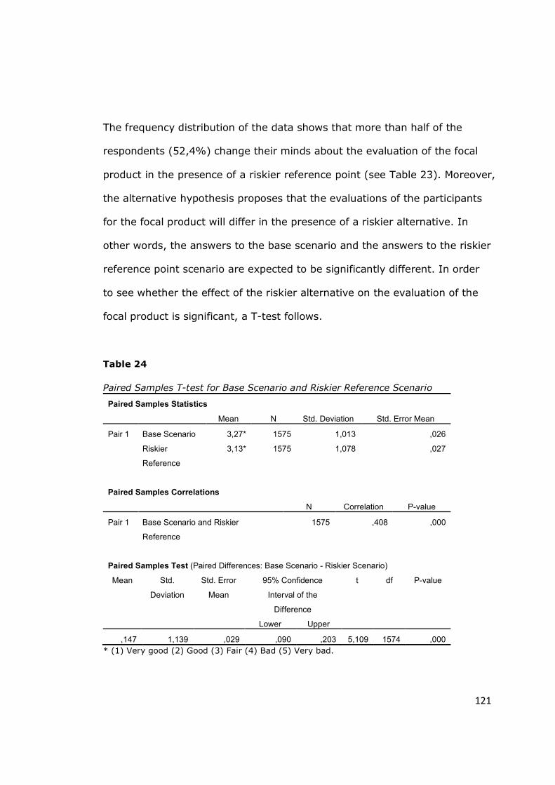
121

The frequency distribution of the data shows that more than half of the

respondents (52,4%) change their minds about the evaluation of the focal

product in the presence of a riskier reference point (see Table 23). Moreover,

the alternative hypothesis proposes that the evaluations of the participants

for the focal product will differ in the presence of a riskier alternative. In

other words, the answers to the base scenario and the answers to the riskier

reference point scenario are expected to be significantly different. In order

to see whether the effect of the riskier alternative on the evaluation of the

focal product is significant, a T-test follows.

Table 24

Paired Samples T-test for Base Scenario and Riskier Reference Scenario

Paired Samples Statistics

Mean N Std. Deviation Std. Error Mean

Pair 1 Base Scenario 3,27* 1575 1,013 ,026

Riskier

Reference

3,13* 1575 1,078 ,027

Paired Samples Correlations

N Correlation P-value

Pair 1 Base Scenario and Riskier

Reference

1575 ,408 ,000

Paired Samples Test (Paired Differences: Base Scenario - Riskier Scenario)

Mean Std.

Deviation

Std. Error

Mean

95% Confidence

Interval of the

Difference

t df P-value

Lower Upper

,147 1,139 ,029 ,090 ,203 5,109 1574 ,000

* (1) Very good (2) Good (3) Fair (4) Bad (5) Very bad.

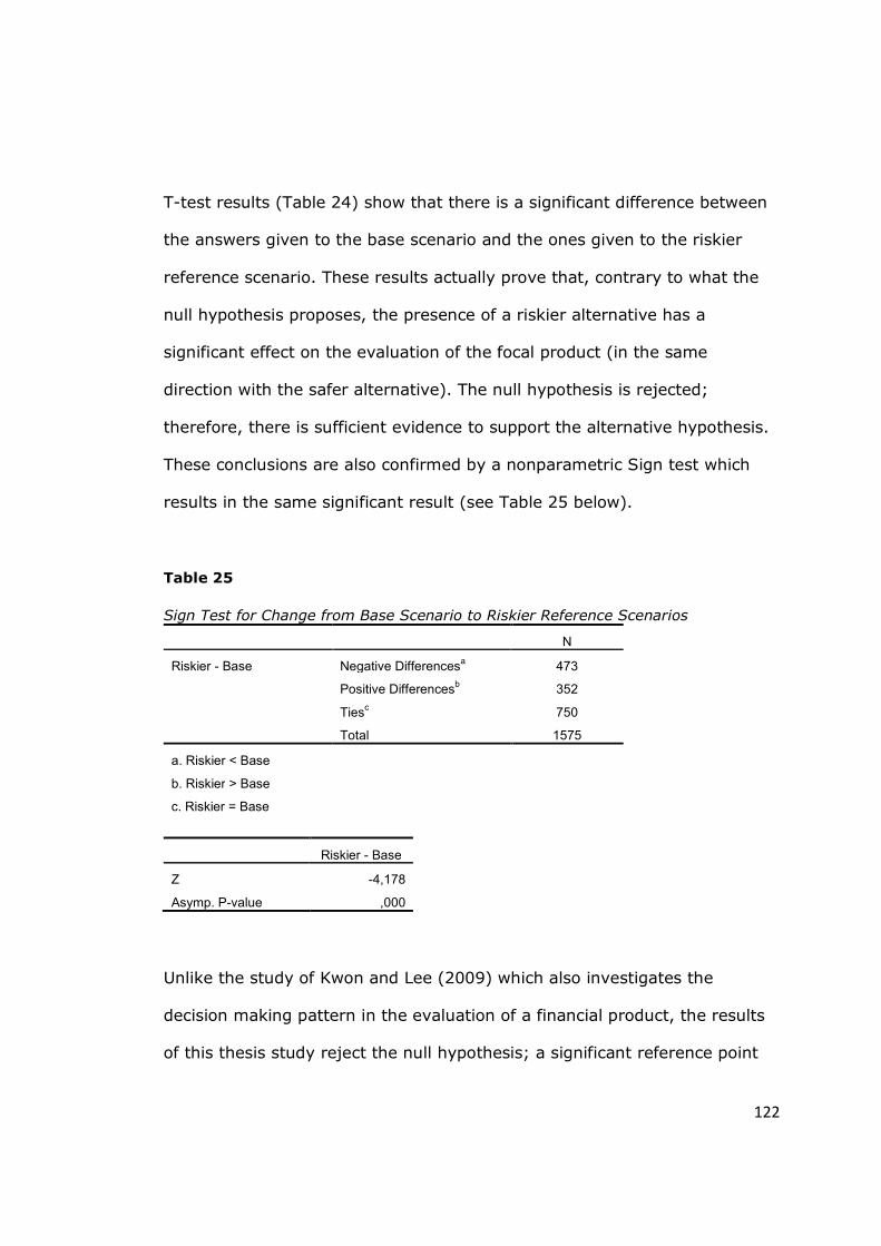
122

T-test results (Table 24) show that there is a significant difference between

the answers given to the base scenario and the ones given to the riskier

reference scenario. These results actually prove that, contrary to what the

null hypothesis proposes, the presence of a riskier alternative has a

significant effect on the evaluation of the focal product (in the same

direction with the safer alternative). The null hypothesis is rejected;

therefore, there is sufficient evidence to support the alternative hypothesis.

These conclusions are also confirmed by a nonparametric Sign test which

results in the same significant result (see Table 25 below).

Table 25

Sign Test for Change from Base Scenario to Riskier Reference Scenarios

N

Riskier - Base Negative Differencesa 473

Positive Differencesb 352

Tiesc 750

Total 1575

a. Riskier < Base

b. Riskier > Base

c. Riskier = Base

Riskier - Base

Z -4,178

Asymp. P-value ,000

Unlike the study of Kwon and Lee (2009) which also investigates the

decision making pattern in the evaluation of a financial product, the results

of this thesis study reject the null hypothesis; a significant reference point

123

effect is found in the presence of a riskier alternative as it is found in the

presence of a safer alternative.

Explicit reference points are used in this study to test the effect of the bias

as Dholakia and Simonson (2005) do. What Tversky and Kahneman (1991)

and Simonson and Tversky (1992) theoretically, and Hsee and Leclerc (1998)

experimentally show is supported by the rejection of the null hypothesis of

Hypothesis 3 and the acceptance of the alternative hypothesis of Hypothesis

2 of this study; reference point is always in effect, no matter which

alternative is the winner. Riskier reference point is also shown to lead the

participants to a better evaluation as safer reference point does. Brenner,

Rottenstreich, and Sood (1999) also support this result by inspecting the

reference point effect in the context of comparisons. They show that what

really matters is the presence of any kind of alternatives (safer or riskier); a

comparison environment with better or worse options is shown to hurt the

evaluation of the focal product, on the other hand.

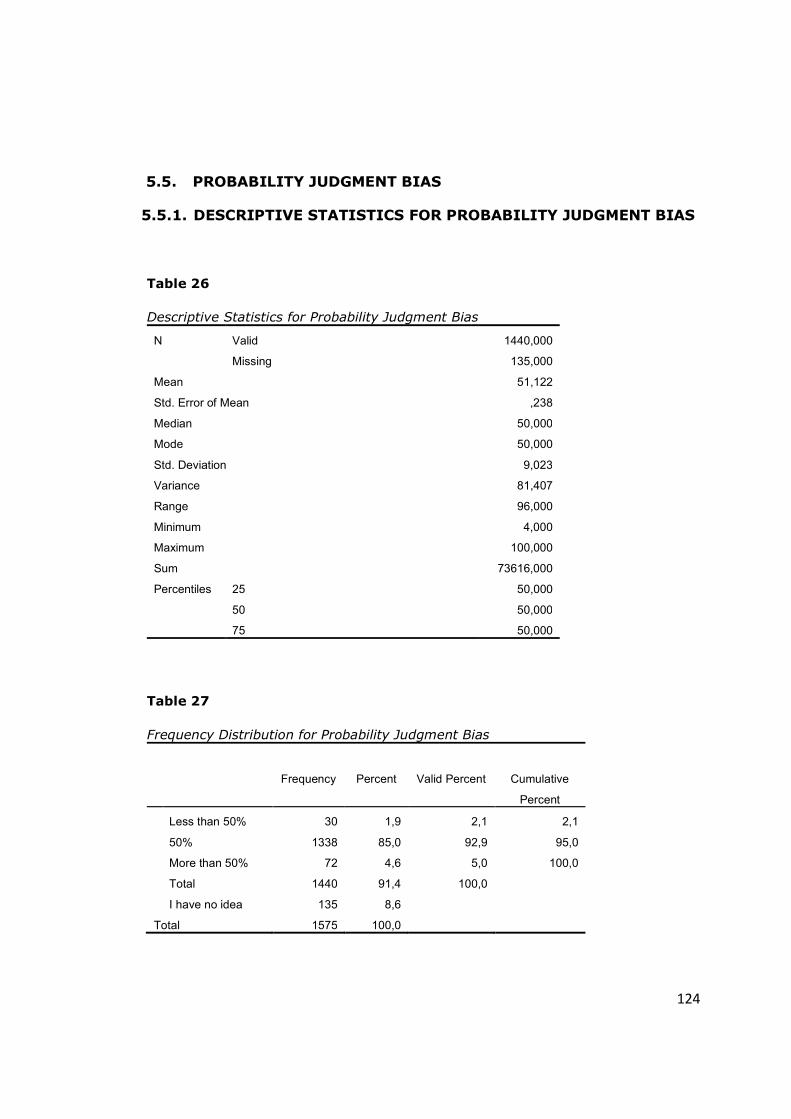
124

5.5. PROBABILITY JUDGMENT BIAS

5.5.1. DESCRIPTIVE STATISTICS FOR PROBABILITY JUDGMENT BIAS

Table 26

Descriptive Statistics for Probability Judgment Bias

N Valid 1440,000

Missing 135,000

Mean 51,122

Std. Error of Mean ,238

Median 50,000

Mode 50,000

Std. Deviation 9,023

Variance 81,407

Range 96,000

Minimum 4,000

Maximum 100,000

Sum 73616,000

Percentiles 25 50,000

50 50,000

75 50,000

Table 27

Frequency Distribution for Probability Judgment Bias

Frequency Percent Valid Percent Cumulative

Percent

Less than 50% 30 1,9 2,1 2,1

50% 1338 85,0 92,9 95,0

More than 50% 72 4,6 5,0 100,0

Total 1440 91,4 100,0

I have no idea 135 8,6

Total 1575 100,0

125

As the frequency distribution (Table 27) shows clearly, and the mode and

the median values of the data confirm accordingly; the most frequent

answer is the correct one, 50%. The mean is %51,122 and it is slightly

above the correct answer (see Table 26). This might mean that the results

show a tendency to gambler’s fallacy; however, the difference is too small to

comment on it. 85% of the respondents give the correct answer, and

excluding the ones who do not answer the question, only 6,5% of the

respondents give wrong answers.

5.5.2. HYPOTHESES ON PROBABILITY JUDGMENT BIAS

Hypothesis 4

H40: There will not be a significant difference between gambler’s fallacy and

hot hand fallacy.

H41: There will be a significant difference between gambler’s fallacy and hot

hand fallacy.

Probability judgment is tested by the fifth question of the original

questionnaire of this study. The respondents are expected to answer the

question either by writing down a prediction of the probability of tails or by

choosing the option “I have no idea.” “I have no idea” option is coded as “0”

since there are no given answers of “0” which is written down as a

prediction. Then, zeros are excluded from the analysis and the data are

recoded by a SPSS 16 syntax8.

8 recode Question5Original (0=.)(1 thru 49=1)(50=2)(51 thru 100=3) into Question5.

126

By this way, the answers are converted into digits, ranging from “1” to “4.”

The digit “1” corresponds to the participants who are biased towards hot

hand fallacy (<%50), and “3” corresponds to the participants who are

biased towards gambler’s fallacy (>%50). Digit “2” corresponds to the

correct objective Bayesian probability judgment which yields a calculation of

50%. Accordingly, the frequency table of the new data set is created (see

Table 27 on page 124).

The respondents who give answers below 50% might be biased towards hot

hand fallacy and the ones who give answers above 50% might be biased

towards gambler’s fallacy. However, as the frequency distribution shows

clearly, the most frequent answer is the correct one, 50%. The mean is

51,122% and it is slightly above the correct answer. In order to see whether

50% is significantly different from 51,122% (whether there is any bias in

the judgment of probability), a proportion test follows. According to the

proportion test, there is no significant difference between these percentages

(chi-square is 0,025181 and p-value is 0,873917). This means that the

respondents are not actually biased in judgment of probabilities.

Since the mean is higher than 50%, there might be a slight predominant

effect of gambler’s fallacy; however, since the difference between the

percentage of the participants who show a tendency to hot hand fallacy and

the percentage of the ones who show a tendency to gambler’s fallacy is too

small (2,1% vs. 5,0% accordingly), it is concluded that an analysis on these

127

data might lead to erroneous results. Moreover, the proportion test already

shows that there is not a statistically significant difference between the

proportions 2,1% and 5,0% (chi-square is 1,228 and p-value is 0,267).

Therefore, the null hypothesis is failed to be rejected and the alternative

hypothesis is rejected. There is not a significant difference between

gambler’s fallacy and hot hand fallacy.

There is a strong dominancy of the correct answers since 85% of the

answers are correct. This may be because of the education level of the

respondents. All of the participants have at least a bachelor’s degree, and as

Dohmen, Falk, Huffman, Marklein, and Sunde (2008) show that educated

people are more likely to give correct answers to probability judgment

questions.

Even though there are some contradictory results in different contexts,

almost all previous studies show that people are inclined to be biased in

probability judgments, if not towards gambler’s fallacy but towards hot hand

fallacy (Kahneman and Tversky, 1972; Tversky and Kahneman, 1974;

Camerer, 1987; Clotfelter and Cook, 1993; Dohmen, Falk, Huffman, and

Marklein, and Sunde, 2009). Some of the researchers, on the other hand,

such as Rabin (2002) or Croson and Sundali (2005), do not consider

gambler’s fallacy as an opposite bias of hot hand fallacy. They claim the

possibility of their joint presence, and they also find a statistically significant

bias in probability judgments.

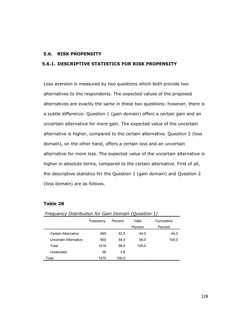
128

5.6. RISK PROPENSITY

5.6.1. DESCRIPTIVE STATISTICS FOR RISK PROPENSITY

Loss aversion is measured by two questions which both provide two

alternatives to the respondents. The expected values of the proposed

alternatives are exactly the same in these two questions; however, there is

a subtle difference: Question 1 (gain domain) offers a certain gain and an

uncertain alternative for more gain. The expected value of the uncertain

alternative is higher, compared to the certain alternative. Question 2 (loss

domain), on the other hand, offers a certain loss and an uncertain

alternative for more loss. The expected value of the uncertain alternative is

higher in absolute terms, compared to the certain alternative. First of all,

the descriptive statistics for the Question 1 (gain domain) and Question 2

(loss domain) are as follows.

Table 28

Frequency Distribution for Gain Domain (Question 1)

Frequency Percent Valid

Percent

Cumulative

Percent

Certain Alternative 669 42,5 44,0 44,0

Uncertain Alternative 850 54,0 56,0 100,0

Total 1519 96,4 100,0

Undecided 56 3,6

Total 1575 100,0

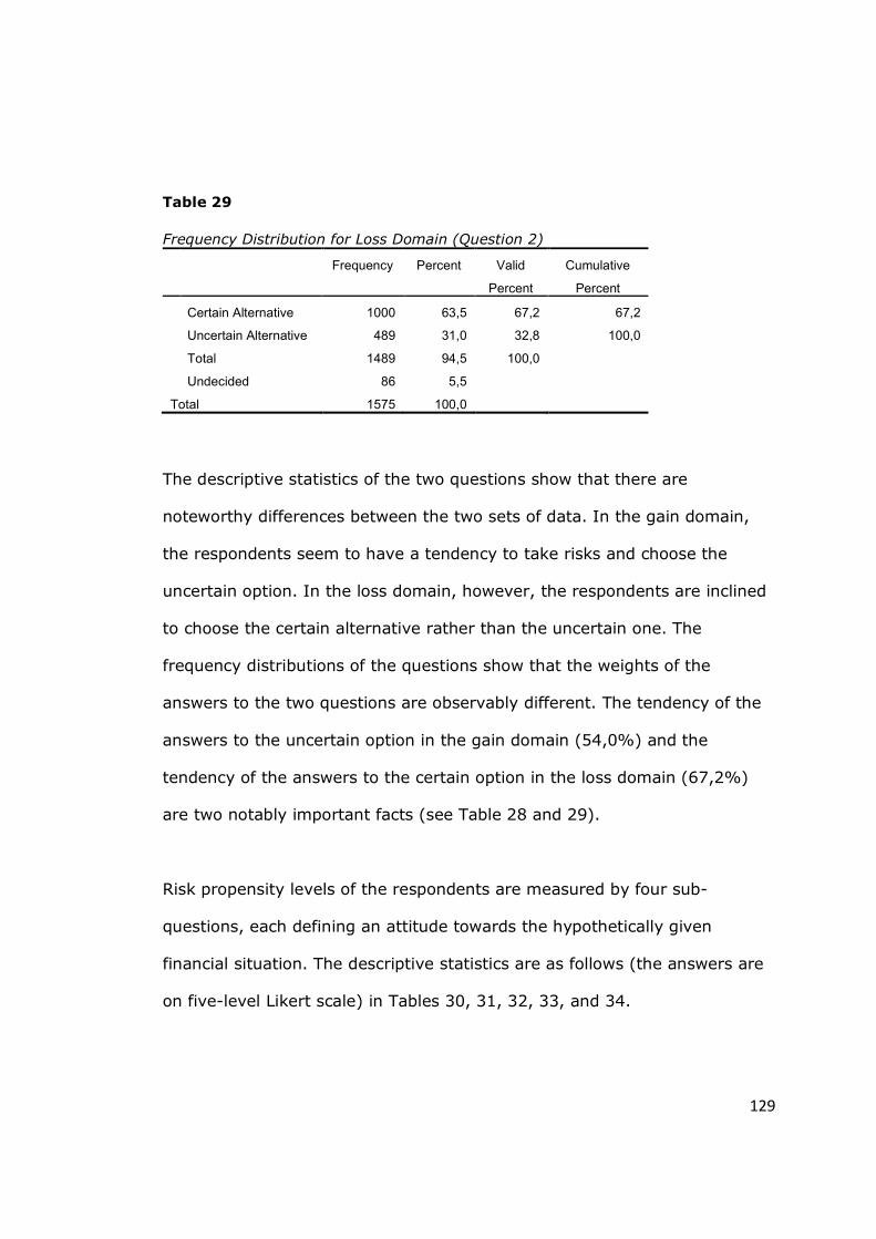
129

Table 29

Frequency Distribution for Loss Domain (Question 2)

Frequency Percent Valid

Percent

Cumulative

Percent

Certain Alternative 1000 63,5 67,2 67,2

Uncertain Alternative 489 31,0 32,8 100,0

Total 1489 94,5 100,0

Undecided 86 5,5

Total 1575 100,0

The descriptive statistics of the two questions show that there are

noteworthy differences between the two sets of data. In the gain domain,

the respondents seem to have a tendency to take risks and choose the

uncertain option. In the loss domain, however, the respondents are inclined

to choose the certain alternative rather than the uncertain one. The

frequency distributions of the questions show that the weights of the

answers to the two questions are observably different. The tendency of the

answers to the uncertain option in the gain domain (54,0%) and the

tendency of the answers to the certain option in the loss domain (67,2%)

are two notably important facts (see Table 28 and 29).

Risk propensity levels of the respondents are measured by four sub-

questions, each defining an attitude towards the hypothetically given

financial situation. The descriptive statistics are as follows (the answers are

on five-level Likert scale) in Tables 30, 31, 32, 33, and 34.

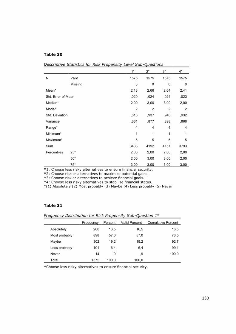
130

Table 30

Descriptive Statistics for Risk Propensity Level Sub-Questions

1* 2* 3* 4*

N Valid 1575 1575 1575 1575

Missing 0 0 0 0

Mean* 2,18 2,66 2,64 2,41

Std. Error of Mean ,020 ,024 ,024 ,023

Median* 2,00 3,00 3,00 2,00

Mode* 2 2 2 2

Std. Deviation ,813 ,937 ,948 ,932

Variance ,661 ,877 ,898 ,868

Range* 4 4 4 4

Minimum* 1 1 1 1

Maximum* 5 5 5 5

Sum 3436 4192 4157 3793

Percentiles 25* 2,00 2,00 2,00 2,00

50* 2,00 3,00 3,00 2,00

75* 3,00 3,00 3,00 3,00

*1: Choose less risky alternatives to ensure financial security. *2: Choose riskier alternatives to maximize potential gains. *3: Choose riskier alternatives to achieve financial goals. *4: Choose less risky alternatives to stabilize financial status. *(1) Absolutely (2) Most probably (3) Maybe (4) Less probably (5) Never

Table 31

Frequency Distribution for Risk Propensity Sub-Question 1* Frequency Percent Valid Percent Cumulative Percent

Absolutely 260 16,5 16,5 16,5

Most probably 898 57,0 57,0 73,5

Maybe 302 19,2 19,2 92,7

Less probably 101 6,4 6,4 99,1

Never 14 ,9 ,9 100,0

Total 1575 100,0 100,0

*Choose less risky alternatives to ensure financial security.

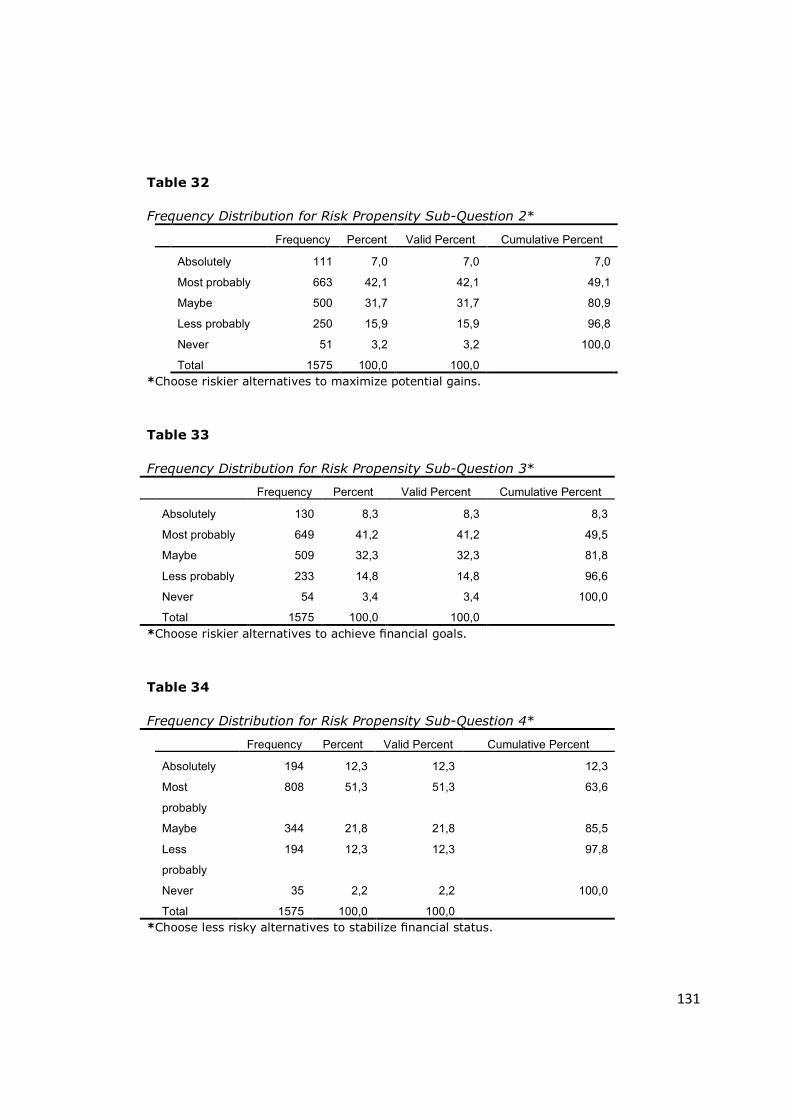
131

Table 32

Frequency Distribution for Risk Propensity Sub-Question 2* Frequency Percent Valid Percent Cumulative Percent

Absolutely 111 7,0 7,0 7,0

Most probably 663 42,1 42,1 49,1

Maybe 500 31,7 31,7 80,9

Less probably 250 15,9 15,9 96,8

Never 51 3,2 3,2 100,0

Total 1575 100,0 100,0

*Choose riskier alternatives to maximize potential gains.

Table 33

Frequency Distribution for Risk Propensity Sub-Question 3* Frequency Percent Valid Percent Cumulative Percent

Absolutely 130 8,3 8,3 8,3

Most probably 649 41,2 41,2 49,5

Maybe 509 32,3 32,3 81,8

Less probably 233 14,8 14,8 96,6

Never 54 3,4 3,4 100,0

Total 1575 100,0 100,0

*Choose riskier alternatives to achieve financial goals.

Table 34

Frequency Distribution for Risk Propensity Sub-Question 4* Frequency Percent Valid Percent Cumulative Percent

Absolutely 194 12,3 12,3 12,3

Most

probably

808 51,3 51,3 63,6

Maybe 344 21,8 21,8 85,5

Less

probably

194 12,3 12,3 97,8

Never 35 2,2 2,2 100,0

Total 1575 100,0 100,0

*Choose less risky alternatives to stabilize financial status.

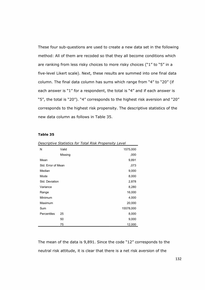
132

These four sub-questions are used to create a new data set in the following

method: All of them are recoded so that they all become conditions which

are ranking from less risky choices to more risky choices (“1” to “5” in a

five-level Likert scale). Next, these results are summed into one final data

column. The final data column has sums which range from “4” to “20” (if

each answer is “1” for a respondent, the total is “4” and if each answer is

“5”, the total is “20”). “4” corresponds to the highest risk aversion and “20”

corresponds to the highest risk propensity. The descriptive statistics of the

new data column as follows in Table 35.

Table 35

Descriptive Statistics for Total Risk Propensity Level

N Valid 1575,000

Missing ,000

Mean 9,891

Std. Error of Mean ,073

Median 9,000

Mode 8,000

Std. Deviation 2,878

Variance 8,280

Range 16,000

Minimum 4,000

Maximum 20,000

Sum 15578,000

Percentiles 25 8,000

50 9,000

75 12,000

The mean of the data is 9,891. Since the code “12” corresponds to the

neutral risk attitude, it is clear that there is a net risk aversion of the

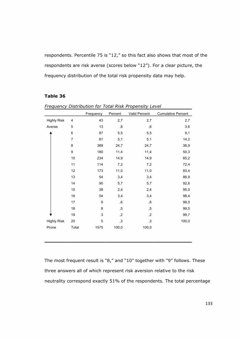
133

respondents. Percentile 75 is “12,” so this fact also shows that most of the

respondents are risk averse (scores below “12”). For a clear picture, the

frequency distribution of the total risk propensity data may help.

Table 36

Frequency Distribution for Total Risk Propensity Level

Frequency Percent Valid Percent Cumulative Percent

Highly Risk

Averse

Highly Risk

Prone

4 43 2,7 2,7 2,7

5 13 ,8 ,8 3,6

6 87 5,5 5,5 9,1

7 81 5,1 5,1 14,2

8 389 24,7 24,7 38,9

9 180 11,4 11,4 50,3

10 234 14,9 14,9 65,2

11 114 7,2 7,2 72,4

12 173 11,0 11,0 83,4

13 54 3,4 3,4 86,9

14 90 5,7 5,7 92,6

15 38 2,4 2,4 95,0

16 54 3,4 3,4 98,4

17 9 ,6 ,6 99,0

18 8 ,5 ,5 99,5

19 3 ,2 ,2 99,7

20 5 ,3 ,3 100,0

Total 1575 100,0 100,0

The most frequent result is “8,” and “10” together with “9” follows. These

three answers all of which represent risk aversion relative to the risk

neutrality correspond exactly 51% of the respondents. The total percentage

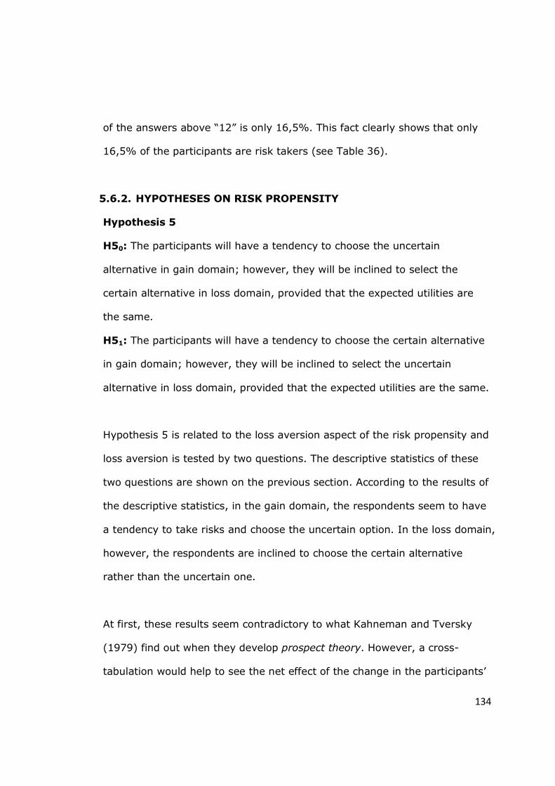
134

of the answers above “12” is only 16,5%. This fact clearly shows that only

16,5% of the participants are risk takers (see Table 36).

5.6.2. HYPOTHESES ON RISK PROPENSITY

Hypothesis 5

H50: The participants will have a tendency to choose the uncertain

alternative in gain domain; however, they will be inclined to select the

certain alternative in loss domain, provided that the expected utilities are

the same.

H51: The participants will have a tendency to choose the certain alternative

in gain domain; however, they will be inclined to select the uncertain

alternative in loss domain, provided that the expected utilities are the same.

Hypothesis 5 is related to the loss aversion aspect of the risk propensity and

loss aversion is tested by two questions. The descriptive statistics of these

two questions are shown on the previous section. According to the results of

the descriptive statistics, in the gain domain, the respondents seem to have

a tendency to take risks and choose the uncertain option. In the loss domain,

however, the respondents are inclined to choose the certain alternative

rather than the uncertain one.

At first, these results seem contradictory to what Kahneman and Tversky

(1979) find out when they develop prospect theory. However, a cross-

tabulation would help to see the net effect of the change in the participants’

135

evaluations of two alternatives in two different domains; namely, the gain

domain and the loss domain (See Table 37).

Table 37

Cross-tabulation Gain Domain * Loss Domain

Question 7

1 2 3 Total

Question 2 1 Count 440 201 28 669

% within Question 2 65,8% 30,0% 4,2% 100,0%

% within Question 7 44,0% 41,1% 32,6% 42,5%

% of Total 27,9% 12,8% 1,8% 42,5%

2 Count 544 275 31 850

% within Question 2 64,0% 32,4% 3,6% 100,0%

% within Question 7 54,4% 56,2% 36,0% 54,0%

% of Total 34,5% 17,5% 2,0% 54,0%

3 Count 16 13 27 56

% within Question 2 28,6% 23,2% 48,2% 100,0%

% within Question 7 1,6% 2,7% 31,4% 3,6%

% of Total 1,0% ,8% 1,7% 3,6%

Total Count 1000 489 86 1575

% within Question 2 63,5% 31,0% 5,5% 100,0%

% within Question 7 100,0% 100,0% 100,0% 100,0%

% of Total 63,5% 31,0% 5,5% 100,0%

The results are more surprising because it seems that the number of the

participants who choose the uncertain alternative in the gain domain and

after change their minds to the certain alternative in the loss domain

constitute the largest percentage (35,5%). On the other hand, the number

of the participants who choose the certain alternative in the gain domain

and after change their minds to the uncertain alternative in the loss domain

constitute only 12,8%. Based on their own article which is published in 1979,

136

Tversky and Kahneman develop a four-fold pattern in 1992. The four-fold

pattern suggests risk aversion for gains and risk seeking behavior for losses

in high probability events. However, it predicts risk seeking behavior for

gains and risk aversion for losses in low probability events (Tversky and

Kahneman, 1992). In this thesis study, the gain domain and the loss domain

both provide high probability alternatives so that the results are in

contradiction to the prospect theory. Moreover, the proportion test shows

that there is a statistically significant difference between the distribution of

the answers for the gain domain and the distribution of the answers for the

loss domain (chi-square is 10,90 and p-value is 0,000961).

The participants who show the same risk preference in both domains

constitute 47,1% of the total subjects. This means that more than half of

the participants evaluate the same alternatives differently depending on

whether it is a gain or a loss environment. This is the second important

outcome of the cross tabulation.

These varying responses to the same choices might be in relation with the

perception of the risk. However, Sitkin and Pablo (1992) build the

theoretical background in order to understand the effects of risk propensity

in detail, and Sitkin and Weingart (1995) support that theoretical

background with their experimental approach. In both of these two studies,

the relationship between risk propensity and perceived risk is found not to

exist significantly. Therefore, the reason is not the perception of the risk.

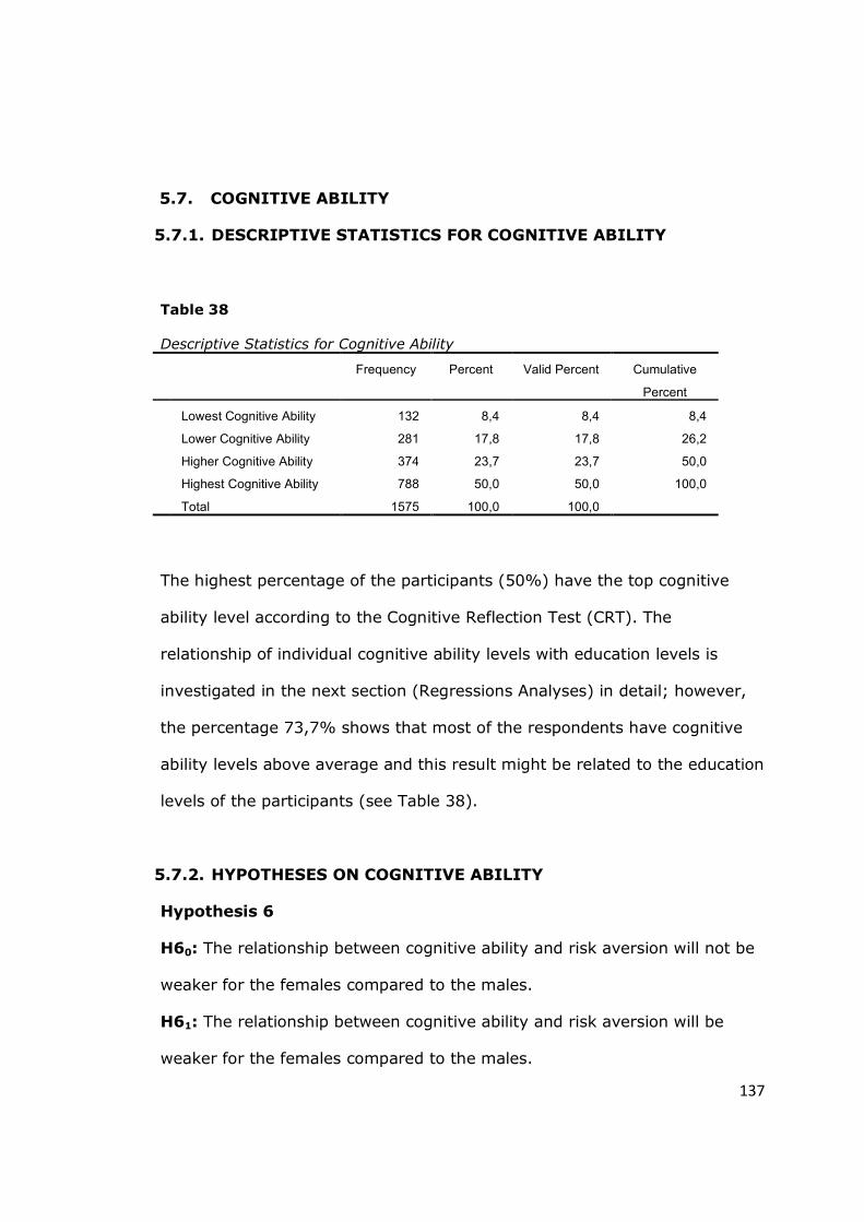
137

5.7. COGNITIVE ABILITY

5.7.1. DESCRIPTIVE STATISTICS FOR COGNITIVE ABILITY

Table 38

Descriptive Statistics for Cognitive Ability

Frequency Percent Valid Percent Cumulative

Percent

Lowest Cognitive Ability 132 8,4 8,4 8,4

Lower Cognitive Ability 281 17,8 17,8 26,2

Higher Cognitive Ability 374 23,7 23,7 50,0

Highest Cognitive Ability 788 50,0 50,0 100,0

Total 1575 100,0 100,0

The highest percentage of the participants (50%) have the top cognitive

ability level according to the Cognitive Reflection Test (CRT). The

relationship of individual cognitive ability levels with education levels is

investigated in the next section (Regressions Analyses) in detail; however,

the percentage 73,7% shows that most of the respondents have cognitive

ability levels above average and this result might be related to the education

levels of the participants (see Table 38).

5.7.2. HYPOTHESES ON COGNITIVE ABILITY

Hypothesis 6

H60: The relationship between cognitive ability and risk aversion will not be

weaker for the females compared to the males.

H61: The relationship between cognitive ability and risk aversion will be

weaker for the females compared to the males.

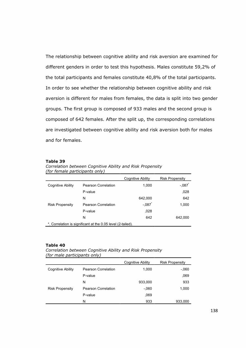
138

The relationship between cognitive ability and risk aversion are examined for

different genders in order to test this hypothesis. Males constitute 59,2% of

the total participants and females constitute 40,8% of the total participants.

In order to see whether the relationship between cognitive ability and risk

aversion is different for males from females, the data is split into two gender

groups. The first group is composed of 933 males and the second group is

composed of 642 females. After the split up, the corresponding correlations

are investigated between cognitive ability and risk aversion both for males

and for females.

Table 39 Correlation between Cognitive Ability and Risk Propensity

(for female participants only)

Cognitive Ability Risk Propensity

Cognitive Ability Pearson Correlation 1,000 -,087*

P-value ,028

N 642,000 642

Risk Propensity Pearson Correlation -,087* 1,000

P-value ,028

N 642 642,000

*. Correlation is significant at the 0.05 level (2-tailed).

Table 40 Correlation between Cognitive Ability and Risk Propensity

(for male participants only)

Cognitive Ability Risk Propensity

Cognitive Ability Pearson Correlation 1,000 -,060

P-value ,069

N 933,000 933

Risk Propensity Pearson Correlation -,060 1,000

P-value ,069

N 933 933,000

139

Contrary to what Dohmen, Falk, Huffman, and Sunde (2010) show, the

correlation between cognitive ability and risk propensity is stronger for

females than males, not the reverse. The Pearson correlations are negative;

therefore, cognitive ability is in direct proportion with risk aversion. As

cognitive ability level increases for an individual, risk aversion also increases.

It can be concluded that the relationship between cognitive ability and risk

aversion is stronger for the females compared to the males (Pearson

correlation coefficients are -0,087 and -0,060 correspondingly). Therefore,

the null hypothesis is failed to be rejected and the alternative hypothesis is

rejected. What is more, the correlation between cognitive ability and risk

propensity is significant for females at the 0,05 level (two-tailed) but it is

not significant for males at this level (see Table 39 and 40).

140

5.8. REGRESSIONS

Age, gender, education, income, employment, cognitive ability, (safer)

reference point bias, probability judgment bias, and risk propensity are all of

the variables which are used in regressions. Among them, cognitive ability,

(safer) reference point bias, probability judgment bias, and risk propensity

will be dependent variables in the corresponding settings.

• Age: Ranging from (18) to (80).

• Gender: Male (0) or Female (1).

• Education: Undergraduate (1), Master’s (2), Doctorate (3).

• Income: Ranging from lower income (1) to higher income (9).

• Employment: Students (0) or Professionals (1).

• Cognitive Ability: Ranging from lower cognitive ability (0) to higher (3).

• (Safer) Reference Point Bias9: None (0) or Present (1).

• Probability Judgment Bias10: None (0) or Present (1).

• Risk Propensity: Ranging from lower risk propensity (4) to higher (20).

9 Respondents who change their mind to a better evaluation in the presence of a safer alternative. 10 Respondents who give an answer other than 50% for the probability of tails a coin toss.

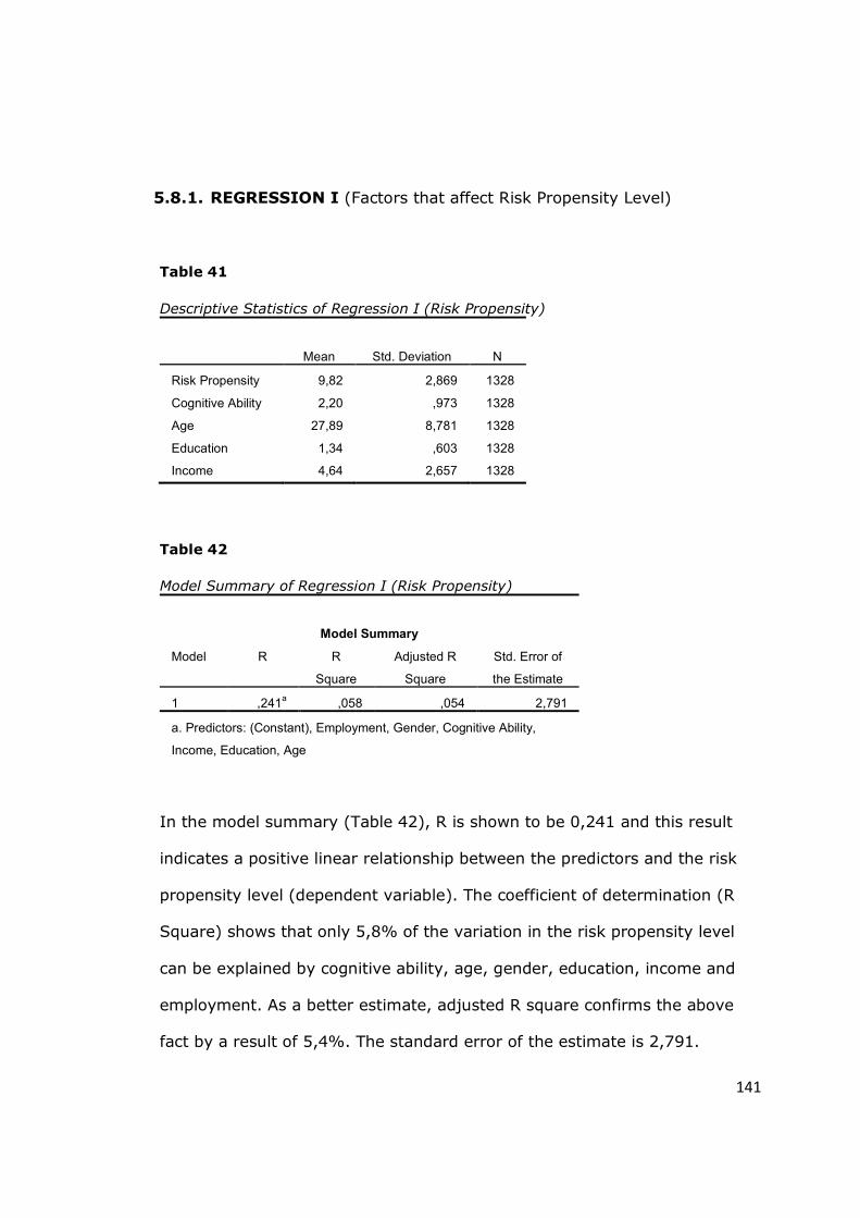
141

5.8.1. REGRESSION I (Factors that affect Risk Propensity Level)

Table 41

Descriptive Statistics of Regression I (Risk Propensity)

Mean Std. Deviation N

Risk Propensity 9,82 2,869 1328

Cognitive Ability 2,20 ,973 1328

Age 27,89 8,781 1328

Education 1,34 ,603 1328

Income 4,64 2,657 1328

Table 42

Model Summary of Regression I (Risk Propensity)

Model Summary

Model R R

Square

Adjusted R

Square

Std. Error of

the Estimate

1 ,241a ,058 ,054 2,791

a. Predictors: (Constant), Employment, Gender, Cognitive Ability,

Income, Education, Age

In the model summary (Table 42), R is shown to be 0,241 and this result

indicates a positive linear relationship between the predictors and the risk

propensity level (dependent variable). The coefficient of determination (R

Square) shows that only 5,8% of the variation in the risk propensity level

can be explained by cognitive ability, age, gender, education, income and

employment. As a better estimate, adjusted R square confirms the above

fact by a result of 5,4%. The standard error of the estimate is 2,791.

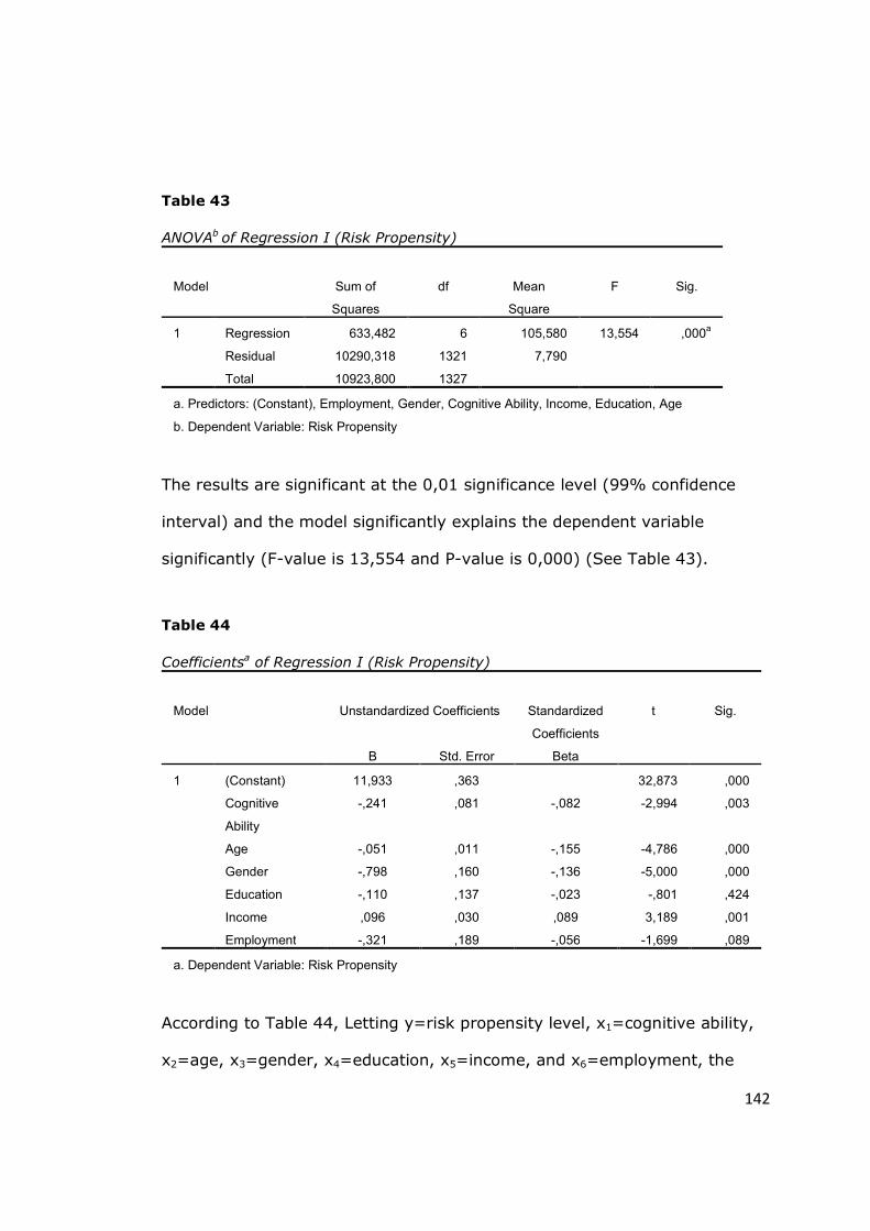
142

Table 43

ANOVAb of Regression I (Risk Propensity)

Model Sum of

Squares

df Mean

Square

F Sig.

1 Regression 633,482 6 105,580 13,554 ,000a

Residual 10290,318 1321 7,790

Total 10923,800 1327

a. Predictors: (Constant), Employment, Gender, Cognitive Ability, Income, Education, Age

b. Dependent Variable: Risk Propensity

The results are significant at the 0,01 significance level (99% confidence

interval) and the model significantly explains the dependent variable

significantly (F-value is 13,554 and P-value is 0,000) (See Table 43).

Table 44

Coefficientsa of Regression I (Risk Propensity)

Model Unstandardized Coefficients Standardized

Coefficients

t Sig.

B Std. Error Beta

1 (Constant) 11,933 ,363 32,873 ,000

Cognitive

Ability

-,241 ,081 -,082 -2,994 ,003

Age -,051 ,011 -,155 -4,786 ,000

Gender -,798 ,160 -,136 -5,000 ,000

Education -,110 ,137 -,023 -,801 ,424

Income ,096 ,030 ,089 3,189 ,001

Employment -,321 ,189 -,056 -1,699 ,089

a. Dependent Variable: Risk Propensity

According to Table 44, Letting y=risk propensity level, x1=cognitive ability,

x2=age, x3=gender, x4=education, x5=income, and x6=employment, the

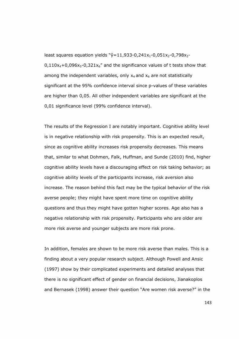
143

least squares equation yields “ŷ=11,933-0,241x1-0,051x2-0,798x3-

0,110x4+0,096x5-0,321x6” and the significance values of t tests show that

among the independent variables, only x4 and x6 are not statistically

significant at the 95% confidence interval since p-values of these variables

are higher than 0,05. All other independent variables are significant at the

0,01 significance level (99% confidence interval).

The results of the Regression I are notably important. Cognitive ability level

is in negative relationship with risk propensity. This is an expected result,

since as cognitive ability increases risk propensity decreases. This means

that, similar to what Dohmen, Falk, Huffman, and Sunde (2010) find, higher

cognitive ability levels have a discouraging effect on risk taking behavior; as

cognitive ability levels of the participants increase, risk aversion also

increase. The reason behind this fact may be the typical behavior of the risk

averse people; they might have spent more time on cognitive ability

questions and thus they might have gotten higher scores. Age also has a

negative relationship with risk propensity. Participants who are older are

more risk averse and younger subjects are more risk prone.

In addition, females are shown to be more risk averse than males. This is a

finding about a very popular research subject. Although Powell and Ansic

(1997) show by their complicated experiments and detailed analyses that

there is no significant effect of gender on financial decisions, Jianakoplos

and Bernasek (1998) answer their question “Are women risk averse?” in the

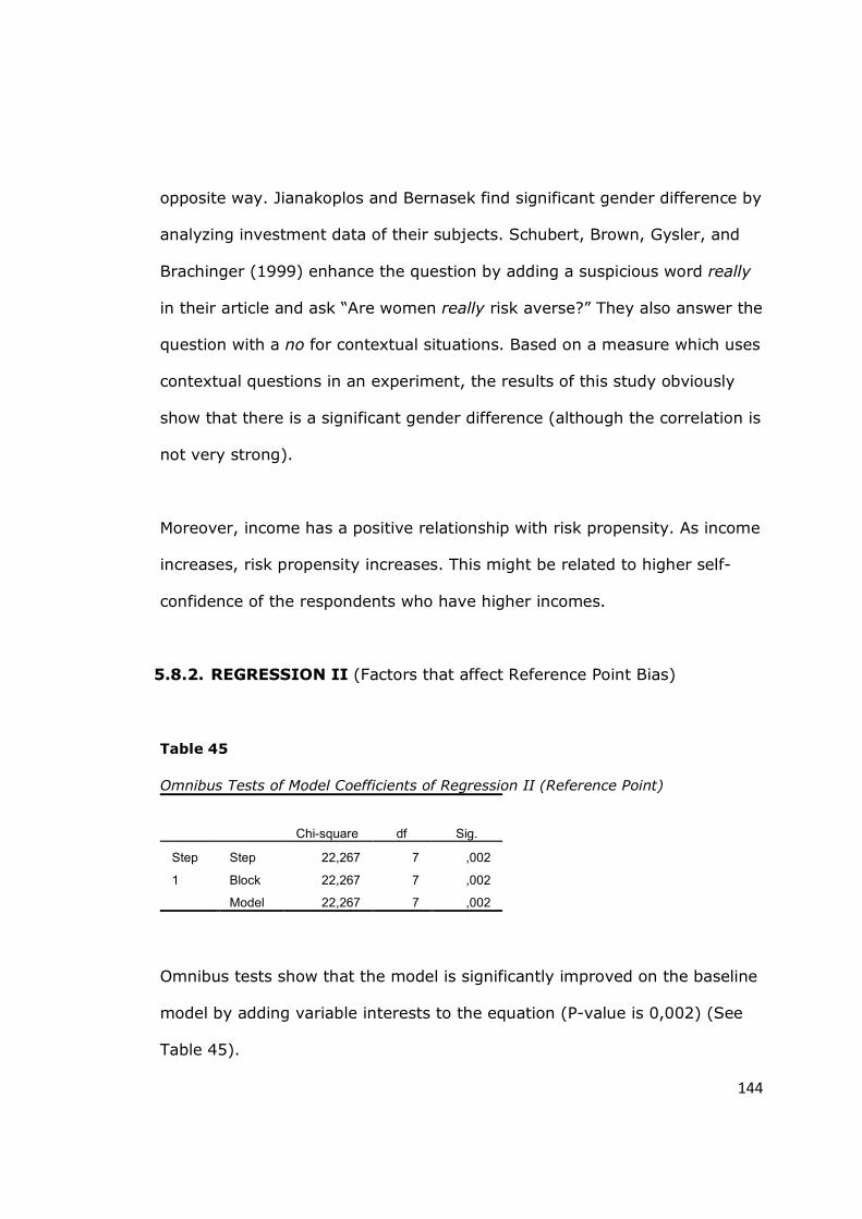
144

opposite way. Jianakoplos and Bernasek find significant gender difference by

analyzing investment data of their subjects. Schubert, Brown, Gysler, and

Brachinger (1999) enhance the question by adding a suspicious word really

in their article and ask “Are women really risk averse?” They also answer the

question with a no for contextual situations. Based on a measure which uses

contextual questions in an experiment, the results of this study obviously

show that there is a significant gender difference (although the correlation is

not very strong).

Moreover, income has a positive relationship with risk propensity. As income

increases, risk propensity increases. This might be related to higher self-

confidence of the respondents who have higher incomes.

5.8.2. REGRESSION II (Factors that affect Reference Point Bias)

Table 45

Omnibus Tests of Model Coefficients of Regression II (Reference Point)

Chi-square df Sig.

Step

1

Step 22,267 7 ,002

Block 22,267 7 ,002

Model 22,267 7 ,002

Omnibus tests show that the model is significantly improved on the baseline

model by adding variable interests to the equation (P-value is 0,002) (See

Table 45).

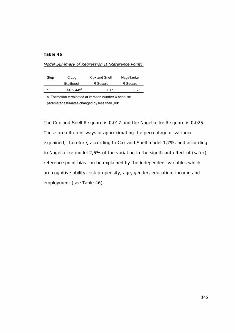
145

Table 46

Model Summary of Regression II (Reference Point)

Step -2 Log

likelihood

Cox and Snell

R Square

Nagelkerke

R Square

1 1462,442a ,017 ,025

a. Estimation terminated at iteration number 4 because

parameter estimates changed by less than ,001.

The Cox and Snell R square is 0,017 and the Nagelkerke R square is 0,025.

These are different ways of approximating the percentage of variance

explained; therefore, according to Cox and Snell model 1,7%, and according

to Nagelkerke model 2,5% of the variation in the significant effect of (safer)

reference point bias can be explained by the independent variables which

are cognitive ability, risk propensity, age, gender, education, income and

employment (see Table 46).

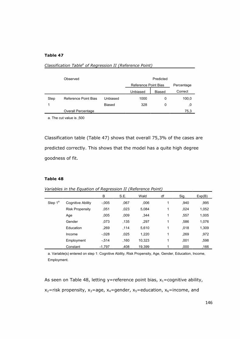
146

Table 47

Classification Tablea of Regression II (Reference Point)

Observed Predicted

Reference Point Bias Percentage

Correct Unbiased Biased

Step

1

Reference Point Bias Unbiased 1000 0 100,0

Biased 328 0 ,0

Overall Percentage 75,3

a. The cut value is ,500

Classification table (Table 47) shows that overall 75,3% of the cases are

predicted correctly. This shows that the model has a quite high degree

goodness of fit.

Table 48

Variables in the Equation of Regression II (Reference Point)

B S.E. Wald df Sig. Exp(B)

Step 1a Cognitive Ability -,005 ,067 ,006 1 ,940 ,995

Risk Propensity ,051 ,023 5,084 1 ,024 1,052

Age ,005 ,009 ,344 1 ,557 1,005

Gender ,073 ,135 ,297 1 ,586 1,076

Education ,269 ,114 5,610 1 ,018 1,309

Income -,028 ,025 1,220 1 ,269 ,972

Employment -,514 ,160 10,323 1 ,001 ,598

Constant -1,797 ,408 19,399 1 ,000 ,166

a. Variable(s) entered on step 1: Cognitive Ability, Risk Propensity, Age, Gender, Education, Income,

Employment.

As seen on Table 48, letting y=reference point bias, x1=cognitive ability,

x2=risk propensity, x3=age, x4=gender, x5=education, x6=income, and

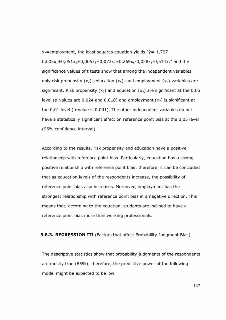
147

x7=employment, the least squares equation yields “ŷ=-1,797-

0,005x1+0,051x2+0,005x3+0,073x4+0,269x5-0,028x6-0,514x7” and the

significance values of t tests show that among the independent variables,

only risk propensity (x2), education (x5), and employment (x7) variables are

significant. Risk propensity (x2) and education (x5) are significant at the 0,05

level (p-values are 0,024 and 0,018) and employment (x7) is significant at

the 0,01 level (p-value is 0,001). The other independent variables do not

have a statistically significant effect on reference point bias at the 0,05 level

(95% confidence interval).

According to the results, risk propensity and education have a positive

relationship with reference point bias. Particularly, education has a strong

positive relationship with reference point bias; therefore, it can be concluded

that as education levels of the respondents increase, the possibility of

reference point bias also increases. Moreover, employment has the

strongest relationship with reference point bias in a negative direction. This

means that, according to the equation, students are inclined to have a

reference point bias more than working professionals.

5.8.3. REGRESSION III (Factors that affect Probability Judgment Bias)

The descriptive statistics show that probability judgments of the respondents

are mostly true (85%); therefore, the predictive power of the following

model might be expected to be low.

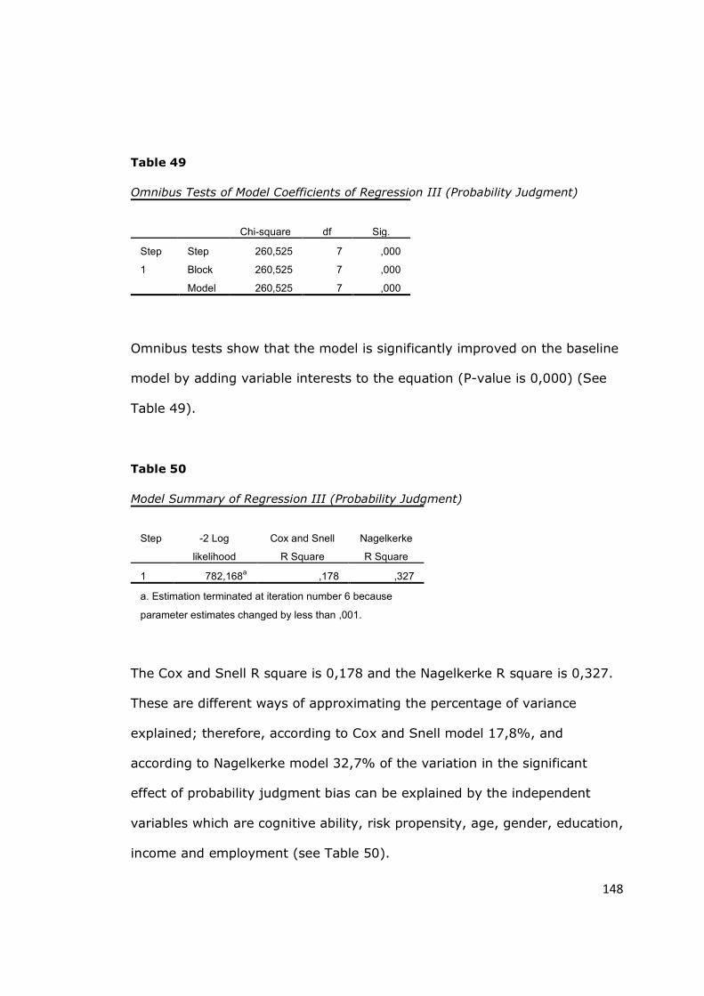
148

Table 49

Omnibus Tests of Model Coefficients of Regression III (Probability Judgment)

Chi-square df Sig.

Step

1

Step 260,525 7 ,000

Block 260,525 7 ,000

Model 260,525 7 ,000

Omnibus tests show that the model is significantly improved on the baseline

model by adding variable interests to the equation (P-value is 0,000) (See

Table 49).

Table 50

Model Summary of Regression III (Probability Judgment)

Step -2 Log

likelihood

Cox and Snell

R Square

Nagelkerke

R Square

1 782,168a ,178 ,327

a. Estimation terminated at iteration number 6 because

parameter estimates changed by less than ,001.

The Cox and Snell R square is 0,178 and the Nagelkerke R square is 0,327.

These are different ways of approximating the percentage of variance

explained; therefore, according to Cox and Snell model 17,8%, and

according to Nagelkerke model 32,7% of the variation in the significant

effect of probability judgment bias can be explained by the independent

variables which are cognitive ability, risk propensity, age, gender, education,

income and employment (see Table 50).

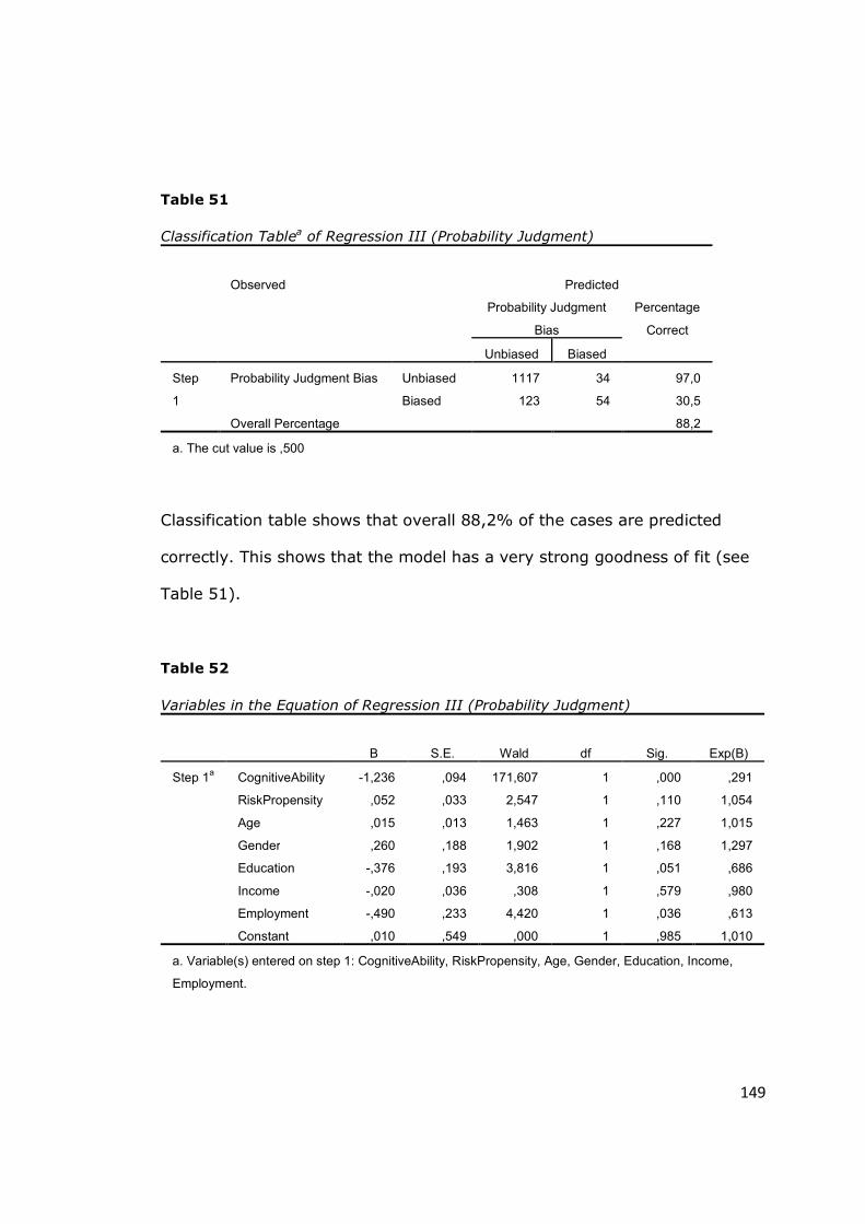
149

Table 51

Classification Tablea of Regression III (Probability Judgment)

Observed Predicted

Probability Judgment

Bias

Percentage

Correct

Unbiased Biased

Step

1

Probability Judgment Bias Unbiased 1117 34 97,0

Biased 123 54 30,5

Overall Percentage 88,2

a. The cut value is ,500

Classification table shows that overall 88,2% of the cases are predicted

correctly. This shows that the model has a very strong goodness of fit (see

Table 51).

Table 52

Variables in the Equation of Regression III (Probability Judgment)

B S.E. Wald df Sig. Exp(B)

Step 1a CognitiveAbility -1,236 ,094 171,607 1 ,000 ,291

RiskPropensity ,052 ,033 2,547 1 ,110 1,054

Age ,015 ,013 1,463 1 ,227 1,015

Gender ,260 ,188 1,902 1 ,168 1,297

Education -,376 ,193 3,816 1 ,051 ,686

Income -,020 ,036 ,308 1 ,579 ,980

Employment -,490 ,233 4,420 1 ,036 ,613

Constant ,010 ,549 ,000 1 ,985 1,010

a. Variable(s) entered on step 1: CognitiveAbility, RiskPropensity, Age, Gender, Education, Income,

Employment.

150

According to Table 52, letting y=probability judgment bias, x1=cognitive

ability, x2=risk propensity, x3=age, x4=gender, x5=education, x6=income,

and x7=employment, the least squares equation yields “ŷ=-0,010-

1,236x1+0,052x2+0,015x3+0,260x4-0,376x5-0,020x6-0,490x7” and the

significance values of t tests show that among the independent variables,

only cognitive ability (x1) and employment (x7) variables are significant (p-

values are 0,000 and 0,036 accordingly). The other independent variables

do not have a statistically significant effect on probability judgments at the

0,05 level (95% confidence interval).

In sum, cognitive ability has a strong negative relationship with biased

probability judgment. Considering the previous studies, this is an expected

result, since as cognitive ability increases the capability of the probability

judgment also increases according to previous researches. As Benjamin,

Brown, and Shapiro (2006) and Oechssler, Roider, and Schmitz (2009) point

out, there is a strong relationship between cognitive ability levels and the

possibility of unbiased decisions.

Another statistically significant variable is employment. The resulting

equation of the Regression III shows that students are inclined to make

biased probability judgments more than working professionals do.

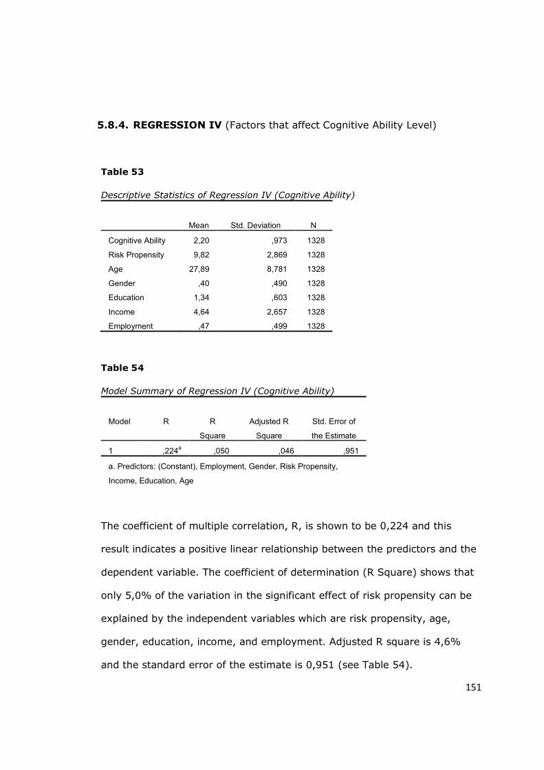
151

5.8.4. REGRESSION IV (Factors that affect Cognitive Ability Level)

Table 53

Descriptive Statistics of Regression IV (Cognitive Ability)

Mean Std. Deviation N

Cognitive Ability 2,20 ,973 1328

Risk Propensity 9,82 2,869 1328

Age 27,89 8,781 1328

Gender ,40 ,490 1328

Education 1,34 ,603 1328

Income 4,64 2,657 1328

Employment ,47 ,499 1328

Table 54

Model Summary of Regression IV (Cognitive Ability)

Model R R

Square

Adjusted R

Square

Std. Error of

the Estimate

1 ,224a ,050 ,046 ,951

a. Predictors: (Constant), Employment, Gender, Risk Propensity,

Income, Education, Age

The coefficient of multiple correlation, R, is shown to be 0,224 and this

result indicates a positive linear relationship between the predictors and the

dependent variable. The coefficient of determination (R Square) shows that

only 5,0% of the variation in the significant effect of risk propensity can be

explained by the independent variables which are risk propensity, age,

gender, education, income, and employment. Adjusted R square is 4,6%

and the standard error of the estimate is 0,951 (see Table 54).

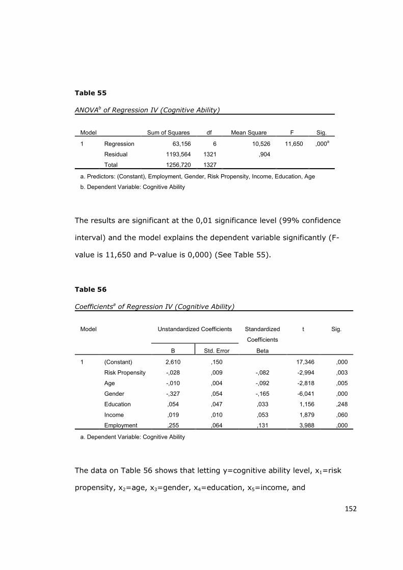
152

Table 55

ANOVAb of Regression IV (Cognitive Ability)

Model Sum of Squares df Mean Square F Sig.

1 Regression 63,156 6 10,526 11,650 ,000a

Residual 1193,564 1321 ,904

Total 1256,720 1327

a. Predictors: (Constant), Employment, Gender, Risk Propensity, Income, Education, Age

b. Dependent Variable: Cognitive Ability

The results are significant at the 0,01 significance level (99% confidence

interval) and the model explains the dependent variable significantly (F-

value is 11,650 and P-value is 0,000) (See Table 55).

Table 56

Coefficientsa of Regression IV (Cognitive Ability)

Model Unstandardized Coefficients Standardized

Coefficients

t Sig.

B Std. Error Beta

1 (Constant) 2,610 ,150 17,346 ,000

Risk Propensity -,028 ,009 -,082 -2,994 ,003

Age -,010 ,004 -,092 -2,818 ,005

Gender -,327 ,054 -,165 -6,041 ,000

Education ,054 ,047 ,033 1,156 ,248

Income ,019 ,010 ,053 1,879 ,060

Employment ,255 ,064 ,131 3,988 ,000

a. Dependent Variable: Cognitive Ability

The data on Table 56 shows that letting y=cognitive ability level, x1=risk

propensity, x2=age, x3=gender, x4=education, x5=income, and

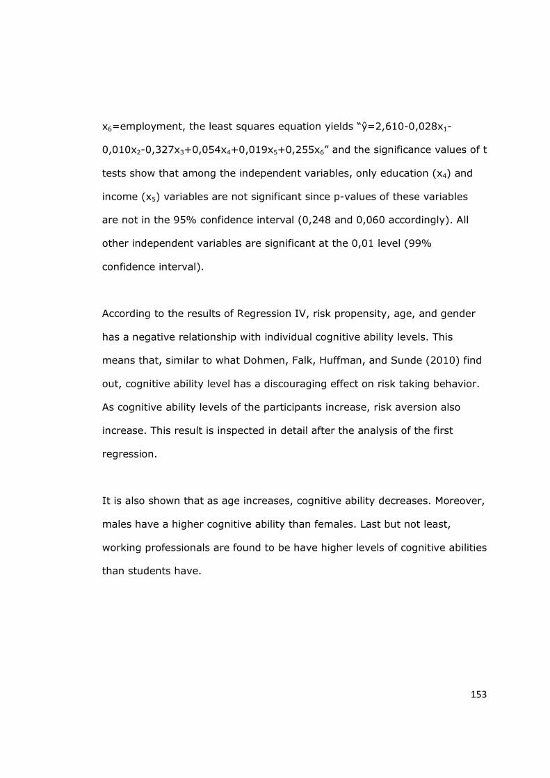
153

x6=employment, the least squares equation yields “ŷ=2,610-0,028x1-

0,010x2-0,327x3+0,054x4+0,019x5+0,255x6” and the significance values of t

tests show that among the independent variables, only education (x4) and

income (x5) variables are not significant since p-values of these variables

are not in the 95% confidence interval (0,248 and 0,060 accordingly). All

other independent variables are significant at the 0,01 level (99%

confidence interval).

According to the results of Regression IV, risk propensity, age, and gender

has a negative relationship with individual cognitive ability levels. This

means that, similar to what Dohmen, Falk, Huffman, and Sunde (2010) find

out, cognitive ability level has a discouraging effect on risk taking behavior.

As cognitive ability levels of the participants increase, risk aversion also

increase. This result is inspected in detail after the analysis of the first

regression.

It is also shown that as age increases, cognitive ability decreases. Moreover,

males have a higher cognitive ability than females. Last but not least,

working professionals are found to be have higher levels of cognitive abilities

than students have.

154

6. DISCUSSION AND CONCLUSION

In sum, the study supports some findings of the previous researches and it

does not support some others. Since the study aims to measure four

different biases and cognitive ability by the same questionnaire, the errors

some of which are mentioned previously might have been occurred. For

instance, the measured variables might have been interacted and this might

have created an undesired biasing effect. However, in brief, the research

contributes to the literature in several aspects. The sample size of the study

is quite big (1575 respondents), the study is carried out in an emerging

country, and the survey is applied to the different groups of participants in

terms of social status, i.e. both students and professionals are included in

the same participant pool. Moreover, the relationships among some

demographic measures, individual cognitive ability levels and behavioral

biases are investigated in the same study.

A questionnaire is designed and used to collect the data. It includes four

question sets which correspond to four selected biases, three questions to

measure cognitive ability, and six questions in order to collect demographics

data (a total of 18 questions). The questions within question sets are in a

mixed order, in order the respondents to be prevented from finding logical

connections between the questions. The purpose of this particular design is

to create an unbiased survey environment. By using SPSS statistical

package version 16, a total of six hypotheses are tested and four

155

regressions are run on two of the selected biases, individual cognitive ability

levels and risk propensity. As an exception, some of the regressions are run

on SPSS version 19 because of the latest version’s enhanced flexibility in

binary logistic regressions.

According to the analyses, anchoring effect is not found at a significant level.

This result is contradictory to most of the previous studies (see Tversky and

Kahneman, 1974; Cervone and Peake, 1986; Johnson and Schkade, 1989;

Jacowitz and Kahneman, 1995; Wilson, Houston, Etling, and Brekke, 1996;

Mussweiler and Strack, 1999; Chapman and Johnson, 1999; Ariely,

Loewenstein, and Prelec, 2003; Oechssler, Roider, and Schmitz, 2009; and

Kudryavtsev and Cohen, 2010). Possible explanations for the contradicting

results might be the complexity of the focal product and the design of the

survey. Participants might have had difficulty in understanding for what they

are bidding exactly. It is also very probable that the presence of several

numbers on the questionnaire might have affected the decisions of the

respondents. Not depending on whether these predictions are true, it would

be wise to extend current research. In order to test anchoring bias correctly,

the design and application of a focused questionnaire on the sole anchoring

subject might be a contribution to the literature. In such a new study, even

though a more tangible focal product might be a better choice, the market

price of it should not be precisely guessed by the participants.

156

In another set of analyses, a safer reference point is found to affect the

financial decisions significantly, compared to the case in which there is no

reference. Moreover, a riskier alternative is also found to affect the financial

decisions of the participants, contrary to a recent study by Kwon and Lee

(2009). Tversky and Kahneman (1991), Simonson and Tversky (1992), and

Hsee and Leclerc (1998) also show that reference points are always in effect

no matter they are safer or riskier compared to the focal product. Although

Brenner, Rottenstreich, and Sood (1999) find out that all references lead to

comparison in the end and they hurt the evaluation of the focal product, the

findings of this thesis study show that reference points make the focal

product more attractive in the context of the evaluation of financial products.

Since the reference point effect is found to be highly dependent on the

context in which it is investigated, further research is suggested in various

contexts to investigate its effect extensively.

Biased probability judgment is another effect which is investigated by the

analyses of the descriptive statistics and a hypothesis. Although most of the

participants (85%) are found to make correct probability judgments for a

toss of a coin and give the correct answer (50%), gambler’s fallacy is shown

to be more frequent than hot hand fallacy. However, since the difference is

not significant and only 6,5% of the participants are found to be biased, the

hypothesis which claims a difference between gambler’s fallacy and hot hand

fallacy is rejected. The result is contradictory to the several previous studies

(e.g., Kahneman and Tversky, 1972; Tversky and Kahneman, 1974;

157

Camerer, 1987; Clotfelter and Cook, 1993; Dohmen, Falk, Huffman, and

Marklein, and Sunde, 2009). Further research by the use of different survey

designs is suggested.

The last behavioral bias which is investigated during the study is risk

propensity. During the analyses of risk propensity, loss aversion is also

tested. There are two questions in the questionnaire which are the two cases

of the same choice condition, one in a gain domain and the other one in a

loss domain. Although the cross-tabulation results of the two questions show

that more than half of the participants change their risk preference while

shifting from the gain domain to the loss domain, the percentage of the

participants who behave in accordance with the loss aversion theory is only

12,8%. Tversky and Kahneman develop loss aversion theory in 1979 and

extend it by explaining four-fold pattern of the theory in 1992. In their

articles, they define a certain loss aversion effect, basing the effect on

several different type of questions; however, this thesis study demonstrate

that the percentage of the respondents who behave in accordance with the

loss aversion theory is quite low. In the risk propensity part of the study,

individual risk propensity levels are also measured. A total of four survey

questions -each of which defining a different risk preference- are combined

into one scale and this scale is used as a demonstration of the individual risk

propensity levels. According to this scale, the participants are found to be

mostly risk averse (72,5%). This is the expected result when it is compared

to the previous studies, for instance, to the study by Sitkin and Weingart

158

(1995) from which the measure is originally taken or to a more recent study

by Kwon and Lee (2009).

The survey of the study also includes the cognitive ability reflection test

(CRT) which is developed by Frederick (2005). Three questions are asked to

the participants and the answers are combined into one a set of data, with a

scale from “0” to “3.” Several different relationships between this final

cognitive ability data set and the other tested variables are investigated. The

results of the analyses on cognitive ability levels of the respondents are

supported by previous researches (Benjamin, Brown, and Shapiro, 2006 and

Oechssler, Roider, and Schmitz, 2009). During the analyses of cognitive

ability, the relationship between cognitive ability and risk propensity is

tested on gender variable. A reverse effect of gender is shown, contrary to

the findings of Dohmen, Falk, Huffman, and Sunde (2010). According to the

results, the correlation between cognitive ability and risk propensity is

stronger for females than males. Moreover, since the correlation for females

is significant and it is not for males, the results need to be reexamined by

extended research which may focus on the measurement of cognitive ability

and risk propensity together with gender.

The regressions also yield interesting results. Cognitive ability level is found

to be in a negative relationship with risk propensity. This is an expected

result, since as cognitive ability increases, risk propensity decreases. In

other words, similar to what Dohmen, Falk, Huffman, and Sunde (2010) find,

159

higher cognitive ability levels have a discouraging effect on risk taking

behavior. In addition, being male is found to be in a positive relationship

with risk propensity; otherwise stated, females are shown to be more risk

averse. Although Powell and Ansic (1997) show by their complicated

experiments and detailed analyses that there is no significant gender effect

on financial decisions, Jianakoplos and Bernasek (1998) answer their

question “Are women risk averse?” in the opposite way. The results of this

thesis study are parallel to what Jianakoplos and Bernasek find out.

Education is found to have a strong positive relationship with reference point

bias. Moreover, employment has the strongest relationship with reference

point bias in a negative direction. This means, students are inclined to have

a reference point bias more than professionals do. Cognitive ability is found

to have a strong negative relationship with biased probability judgment.

Taking the previous studies into consideration, this is an expected result.

Since as Benjamin, Brown, and Shapiro (2006) and Oechssler, Roider, and

Schmitz (2009) point out, there is a strong relationship between higher

cognitive ability levels and unbiased decisions. Moreover, males are found to

have higher cognitive ability levels than females do. Last but not least,

professionals are found to have higher cognitive ability levels than students.

In conclusion, anchoring bias is not found to be statistically significant.

Reference point bias is found to exist in the presence of both safer and

riskier alternatives. On the other hand, probability judgment bias is not

found to significantly exist among the respondents. This result is explained

160

by high education levels of the participants. Loss aversion is not found to

exist in the sample. Moreover, individual risk propensity levels of the

respondents are measured. Biases are, in general, found to be affected by

demographic variables. All these results may provide an initial step for

further research in emerging markets since there have not been enough

studies on the behavioral finance subject until now. In addition, the

indisputable effect of reference points on decision making processes may

have numerous applications in marketing field, and especially in the financial

marketing subfield.

161

REFERENCES

Andersen, J. V. (2010). Detecting anchoring in financial markets. Journal of

Behavioral Finance, 11(2), 129-133. Ariely, D., Loewenstein, G., and Prelec, D. (2003). "Coherent arbitrariness":

Stable demand curves without stable preferences. The Quarterly Journal of Economics, 118(1), 73-105.

Barone, M. J., Rose, R. L., Manning, K. C., and Miniard, P. W. (1996).

Another look at the impact of reference information on consumer impressions of nutrition information. Journal of Public Policy and Marketing, 15(1), 55-62.

Becker, G. S. (1962). Irrational behavior and economic theory. The Journal

of Political Economy, 70(1), 1-13. Benjamin, D. J., Brown, S. A., and Shapiro, J. M. (2006). Who is

“behavioral"? Cognitive ability and anomalous preferences, (May 5, 2006), Available at SSRN: http://ssrn.com/abstract=675264.

Berger, P. O., and Smith, G. E. (1997). The effect of direct mail framing

strategies and segmentation variables on university fundraising performance. Journal of Direct Marketing, 11(Winter), 30-43.

Blackmore, S., and Troscianko, T. (1985). Belief in the paranormal:

Probability judgements, illusory control, and the 'chance baseline shift.” British Journal of Psychology, 76(4), 459-468.

Brañas-Garza, P., Guillen, P., and Rafael López del Paso. (2008). Math skills

and risk attitudes. Economics Letters, 99(2), 332-336. Brenner, L., Rottenstreich, Y., and Sood, S. (1999). Comparison, grouping,

and preference. Psychological Science, 10(3), 225-229. Brockhaus, R. H., Sr. (1980). Risk taking propensity of entrepreneurs. The

Academy of Management Journal, 23(3), 509-520. Brown, J. S. (1970). Risk propensity in decision marking: A comparison of

business and public school administrators. Administrative Science Quarterly, 15(4), 473-481.

Camerer, C. F. (1987). Do biases in probability judgment matter in markets?

Experimental evidence. The American Economic Review, 77(5), 981-997.

162

Cervone, D., and Peake, P. K. (1986). Anchoring, efficacy, and action: The influence of judgmental heuristics on self-efficacy judgments and behavior. Journal of Personality and Social Psychology, 50(3), 492-501.

Chapman, G. B., and Johnson, E. J. (1999). Anchoring, activation, and the

construction of values. Organizational Behavior and Human Decision

Processes, 79(2), 115-153. Chatterjee, S., and Heath, T. B. (1996). Conflict and loss aversion in

multiattribute choice: The effects of trade-off size and reference dependence on decision difficulty. Organizational Behavior and Human

Decision Processes, 67(2), 144-155. Clotfelter, C. T., and Cook, P. J. (1993). "Gambler's fallacy" in lottery play.

Management Science, 39(12), 1521-1525. Croson, R., and Sundali, J. (2005). The gambler’s fallacy and the hot hand:

Empirical data from casinos. The Journal of Risk and Uncertainty, 30(3), 195-209.

Dhar, R., and Nowlis, S. M. (2004). To buy or not to buy: response mode

effects on consumer choice. Journal of Marketing Research, 41(November), 423-443.

Dholakia, U. M., and Simonson, I. (2005). The effect of explicit reference

points on consumer choice and online bidding behavior. Marketing Science, 24(2), 206-217.

Dodonova, A., and Khoroshilov, Y. (2004). Anchoring and transaction utility:

Evidence from on-line auctions. Applied Economics Letters, 11(307), 307-310.

Dohmen, T., Falk, A., Huffman, D., and Sunde, U. (2010). Are risk aversion

and impatience related to cognitive ability? American Economic Review, 100(3), 1238-1260.

Dohmen, T., Falk, A., Huffman, D., Marklein, F., and Sunde, U. (2008). The

economic consequences of biased probability judgment: Representative evidence, mimeo, University of Maastricht.

Dohmen, T., Falk, A., Huffman, D., Marklein, F., and Sunde, U. (2009).

Biased probability judgment: Evidence of incidence and relationship to economic outcomes from a representative sample. Journal of Economic Behavior and Organization, 72, 903-915.

Forbes, W. (2009). Behavioural finance. United Kingdom: Wiley.

163

Frederick, S. (2005). Cognitive reflection and decision making. American Economic Association, 19(4), 25-42.

Hamilton, R. W., and Biehal, G. J. (2005). Achieving your goals or protecting

their future? The effects of self-view on goals and choices. Journal of Consumer Research, 32(2), 277-283.

Harrison, J. D., Young, J. M., Butow, P., Salkeld, G., and Solomon, M. J.

(2005). Is it worth the risk? A systematic review of instruments that measure risk propensityfor use in the health setting. Social Science and Medicine, 60(6), 1385-1396.

Hatfield, J., and Fernandes, R. (2009). The role of risk-propensity in the

risky driving of younger drivers. Accident Analysis and Prevention, 41(1), 25-35.

Helson, H. (1964). Adaptation level theory: An experimental and systematic

approach to behavior. New York: Harper. Howard, D. J., and Kerin, R. A. (2006). Broadening the scope of reference

price advertising research: A field study of consumer shopping involvement. Journal of Marketing, 70(October), 185-204.

Hsee, C. K., and Leclerc, F. (1998). Will products look more attractive when

presented separately or together? The Journal of Consumer Research, 25(2), 175-186.

Huth, P., Bennett, D. S., and Gelpi, C. (1992). System Uncertainty, Risk

Propensity, and International Conflict among the Great Powers. Journal of Conflict Resolution, 36(3), 478-517.

Jacowitz, K. E., and Kahneman, D. (1995). Measures of anchoring in

estimation tasks. Pers Soc Psychol Bull, 21(11), 1161-1166. Jianakoplos, N. A., and Bernasek, A. (1998). Are women more risk averse?

Economic Inquiry, XXXVI, 620-630. Johnson, E. J., and Schkade, D. A. (1989). Bias in utility assessments:

Further evidence and explanations. Management Science, 35(4), 406-424.

Johnson, E. J., Payne, J. W., and Bettman, J. R. (1988). Information

displays and preference reversals. Organizational Behavior and Human Decision Processes, 42, 1-21.

Kahneman, D., and Tversky, A. (1972). Subjective probability: A judgment

of representativeness. Cognitive Psychology, 3, 430-454.

164

Kahneman, D., and Tversky, A. (1979). Prospect theory: An analysis of decision under risk. Econometrica, 47(2), 263-292.

Kai Lai Chung. (2001). A course in probability theory. United States of

America: Academic Press. Kameda, T., and Davis, J. H. (1990). The function of the reference point in

individual and group risk decision making. Organizational Behavior and Human Decision Processes, 46(1), 55-76.

Keil, M., Wallace, L., Turk, D., Dixon-Randall, G., and Nulden, U. (2000). An

investigation of risk perception and risk propensity on the decision to continue a software development project. The Journal of Systems and Software, 53(2), 145-157.

Khoroshilov, Y., and Dodonova, A. (2007). Buying winners while holding on

to losers: An experimental study of investors’ behavior. Economics

Bulletin, 7(8), 1-8. Killgore, W. D. S., Vo, A. H., Castro, C. A., and Hoge, C. W. (2006).

Assessing risk propensity in American soldiers - preliminary reliability and validity of the evaluation of risks (evar) scale. Military Medicine, 171(3), 233-239.

Kudryavtsev, A., and Cohen, G. (2010). Anchoring and pre-existing

knowledge in economic and financial settings. American Journal Of Social And Management Sciences, 1(2), 164-180.

Kwon, K., and Lee, J. (2009). The effects of reference point, knowledge, and

risk propensity on the evaluation of financial products. Journal of Business Research, 62, 719-725.

Massad, V. J., and Reardon, J. (1996). Channel surfing, brand loyalty and

risk propensity: A segmentation approach to modelling consumer switching Behaviours in the USA. International Journal of Advertising, 15(3), 250-261.

Miner, J. B., and Raju, N. S. (2004). Risk propensity differences between

managers and entrepreneurs and between low- and high-growth entrepreneurs: A reply in a more conservative vein. Journal of Applied Psychology, 89(1), 3-13.

Mussweiler, T., and Strack, F. (1999). Comparing is believing: A selective

accessibility model of judgmental anchoring. European Review of Social Psychology, 10(1), 135-167.

165

Northcraft, G. B., and Neale, M. A. (1987). Experts, amateurs, and real estate: An anchoring and adjustment perspective on property pricing decisions. Organizational Behavior and Human Decision Processes, 39(1), 84-97.

Oechssler, J., Roider, A., and Schmitz, P. W. (2009). Cognitive abilities and

behavioral biases. Journal of Economic Behavior and Organization, 72, 147-152.

Palich, L. E., and Bagby, R. (1995). Using cognitive theory to explain

entrepreneurial risk-taking: Challenging conventional wisdom. Journal of Business Venturing, 10(6), 425-438.

Powell, M., and Ansic, D. (1997). Gender differences in risk behaviour in

financial decision-making: An experimental analysis. Journal of Economic Psychology, 18, 605-628.

Rabin, M. (2002). Inference by believers in the law of small numbers. The

Quarterly Journal of Economics, 117(3), 775-816. Redelmeier, DA, Koehler, DJ, Liberman, V, and Tversky, A. (1995).

Probability judgement in medicine: discounting unspecified possibilities. Medical Decision Making, 15(3), 227-230.

Schubert, R., Brown, M., Gysler, M., and Brachinger. (1999). Financial

decision-making: Are women really more risk-averse? The American Economic Review, 89(2), 381-385.

Selden, G. C. (1912). Psychology of the Stock Market: Human Impulses

Lead To Speculative Disasters. New York: Ticker Publishing Sharma, S., and Nguan, O. (1999). The biotechnology industry and

strategies of biodiversity conservation: The influence of managerial interpretations and risk propensity. Business Strategy and the Environment, 8(1), 46-61.

Shefrin, H. (2005). A behavioral approach to asset pricing. New York:

Elsevier. Shefrin, H. M., and Statman, M. (1985). The disposition to sell winners too

early and rise losers too long. Journal of Finance, 40, 770-777. Shleifer, A. (2004). Inefficient markets: An introduction to behavioral

finance. New York: Oxford University Press.

166

Siegmund, D. O. (2011). Probability theory (mathematics) -- britannica online encyclopedia. United States: Encyclopædia Britannica, Inc. Retrieved from http://www.britannica.com/EBchecked/topic/477530/probability-theory

Simon, M., Houghton, S. M., and Aquino, K. (1999). Cognitive biases, risk

perception, and venture formation: How individuals decide to start companies. Journal of Business Venturing, 15, 113-134.

Simonson, I., and Tversky, A. (1992). Choice in context: Tradeoff contrast

and extremeness aversion. Journal of Marketing Research, XXIX, 281-295.

Sitkin, S. B., and Pablo, A. L. (1992). Reconceptualizing the determinants of

risk behavior. The Academy of Management Review, 17(1), 9-38. Sitkin, S. B., and Weingart, L. R. (1995). Determinants of risky decision-

making behavior: A test of the mediating role of risk perceptions and propensity. The Academy of Management Journal, 38(6), 1573-1592.

Slonim, R., Carlson, J., and Bettinger, E. (2007). Possession and discounting

behavior. Economics Letters, 97, 215-221. Slovic, P., and Lichtenstein, S. (1971). Comparison of bayesian and

regression approaches to the study of information processing in judgment. Organizational Behavior and Human Performance, 6(6), 649-744.

Tversky, A, and Kahneman, D. (1996). Loss aversion in riskless choice: a

reference-dependent model. The Quarterly Journal of Economics, 106(4), 1039-1061.

Tversky, A., and Kahneman, D. (1973). Availability: A heuristic for judging

frequency and probability. Cognitive Psychology, 5(2), 207-232. Tversky, A., and Kahneman, D. (1974). Judgment under uncertainty:

Heuristics and biases. Science, 185. Tversky, A., and Kahneman, D. (1991). Loss aversion in riskless choice: A

reference-dependent model. The Quarterly Journal of Economics, 106(4), 1039-1061.

Tversky, A., and Kahneman, D. (1992). Advances in prospect

theory:Cumulative representation of uncertainty. Journal of Risk and Uncertainty, 5, 297-323.

167

Tversky, A., and Simonson, I. (1993). Context-dependent preferences. Management Science, 39(10), 1179-1189.

Walls, M. R., and Dyer, J. S. (1996). Risk propensity and firm performance:

A study of the petroleum exploration industry. Management Science, 42(7), 1004-1021.

Wilson, T. D., Houston, C. E., Etling, K. M., and Brekke, N. (1996). A new

look at anchoring effects: Basic anchoring and its antecedents. Journal of Experimental Psychology, 125(4), 387-402.

Wright, W. F., and Bower, G. H. (1992). Mood effects on subjective

probability assessment. Organizational Behavior and Human Decision Processes, 52(2), 276-291.

Yates, J. F., Zhu, Y., Ronis, D. L., Wang, D., Shinotsuka, H., and Toda, M.

(1989). Probability judgment accuracy: China, Japan, and the United States. Organizational Behavior and Human Decision Processes, 43(2), 145-171.

Ye, G. (2004). Inertia equity: The impact of anchoring price in brand

switching. Available at SSRN: http://ssrn.com/abstract=548862. Zhang, Y, and Mittal, V. (2005). Decision difficulty: effects of procedural and

outcome accountability. Journal of Consumer Research, 32(Dec.), 465-472.

.

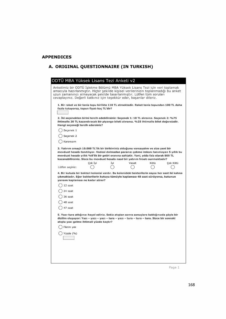
168

APPENDICES

A. ORIGINAL QUESTIONNAIRE (IN TURKISH)

169

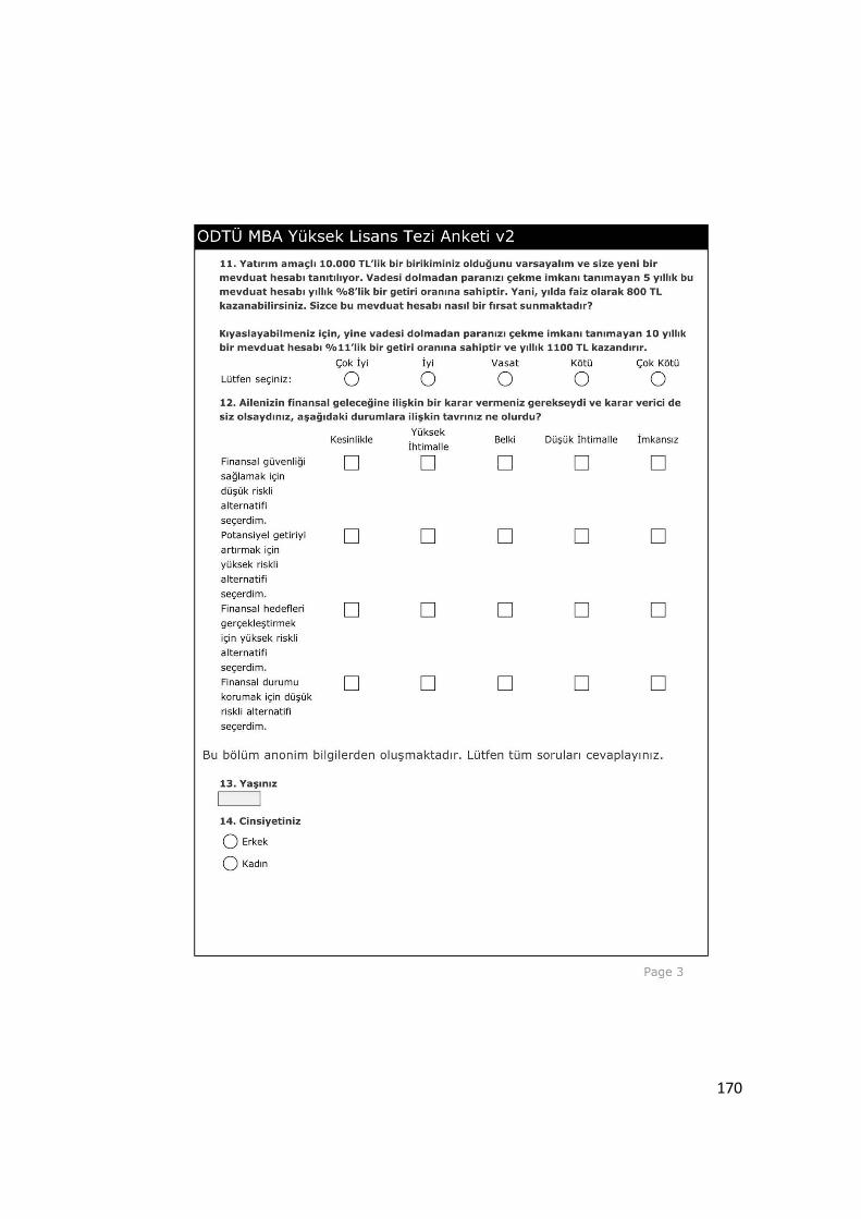
170

171

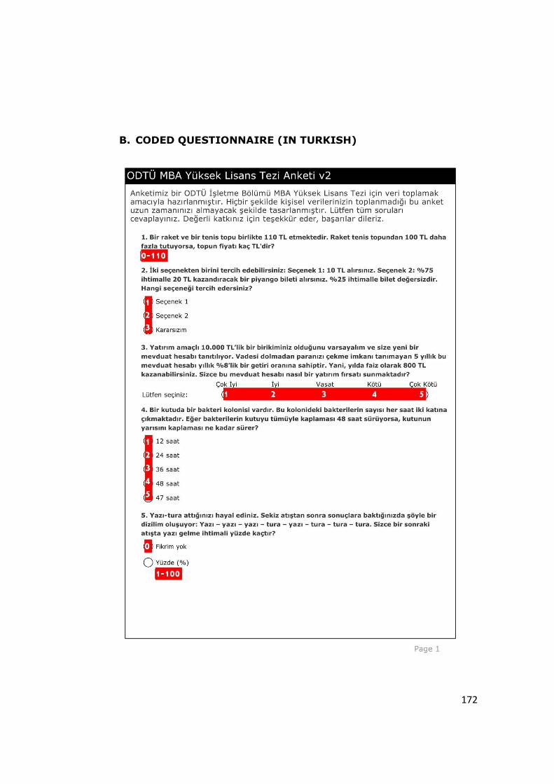
172

B. CODED QUESTIONNAIRE (IN TURKISH)

173

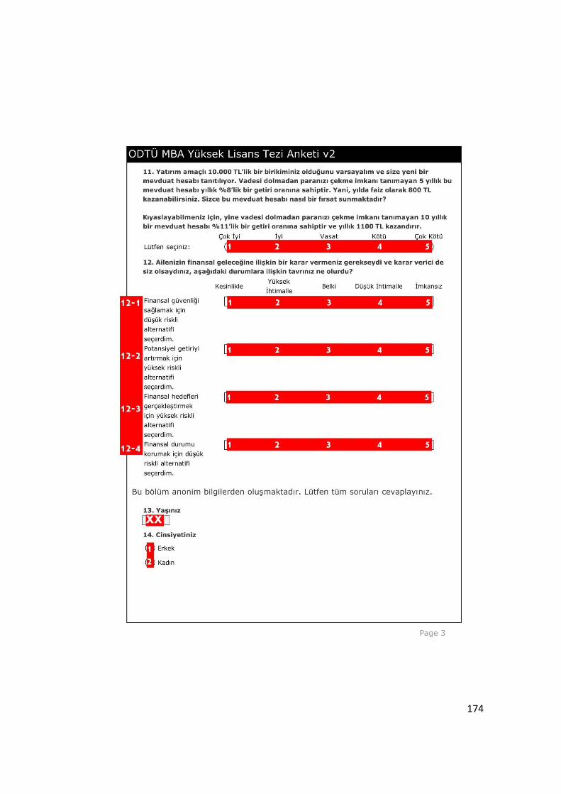
174

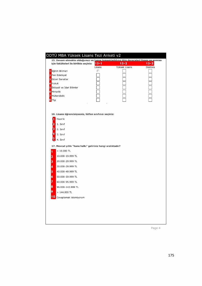
175

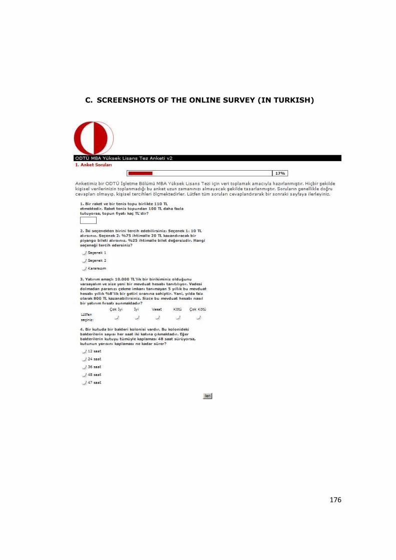
176

C. SCREENSHOTS OF THE ONLINE SURVEY (IN TURKISH)

177

178

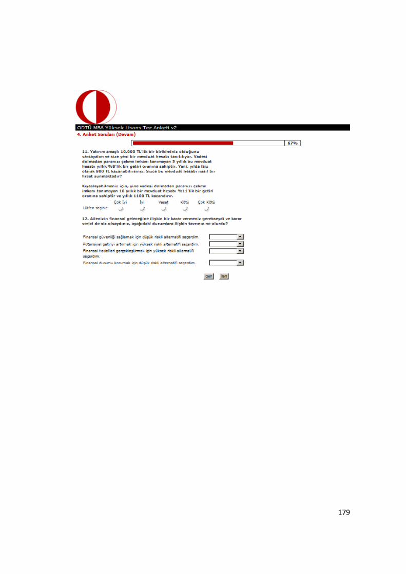
179

180

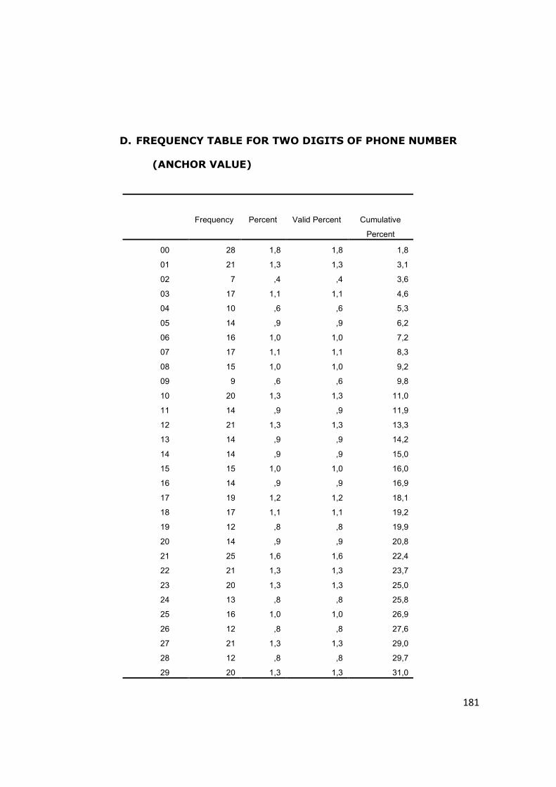
181

D. FREQUENCY TABLE FOR TWO DIGITS OF PHONE NUMBER

(ANCHOR VALUE)

Frequency Percent Valid Percent Cumulative

Percent

00 28 1,8 1,8 1,8

01 21 1,3 1,3 3,1

02 7 ,4 ,4 3,6

03 17 1,1 1,1 4,6

04 10 ,6 ,6 5,3

05 14 ,9 ,9 6,2

06 16 1,0 1,0 7,2

07 17 1,1 1,1 8,3

08 15 1,0 1,0 9,2

09 9 ,6 ,6 9,8

10 20 1,3 1,3 11,0

11 14 ,9 ,9 11,9

12 21 1,3 1,3 13,3

13 14 ,9 ,9 14,2

14 14 ,9 ,9 15,0

15 15 1,0 1,0 16,0

16 14 ,9 ,9 16,9

17 19 1,2 1,2 18,1

18 17 1,1 1,1 19,2

19 12 ,8 ,8 19,9

20 14 ,9 ,9 20,8

21 25 1,6 1,6 22,4

22 21 1,3 1,3 23,7

23 20 1,3 1,3 25,0

24 13 ,8 ,8 25,8

25 16 1,0 1,0 26,9

26 12 ,8 ,8 27,6

27 21 1,3 1,3 29,0

28 12 ,8 ,8 29,7

29 20 1,3 1,3 31,0

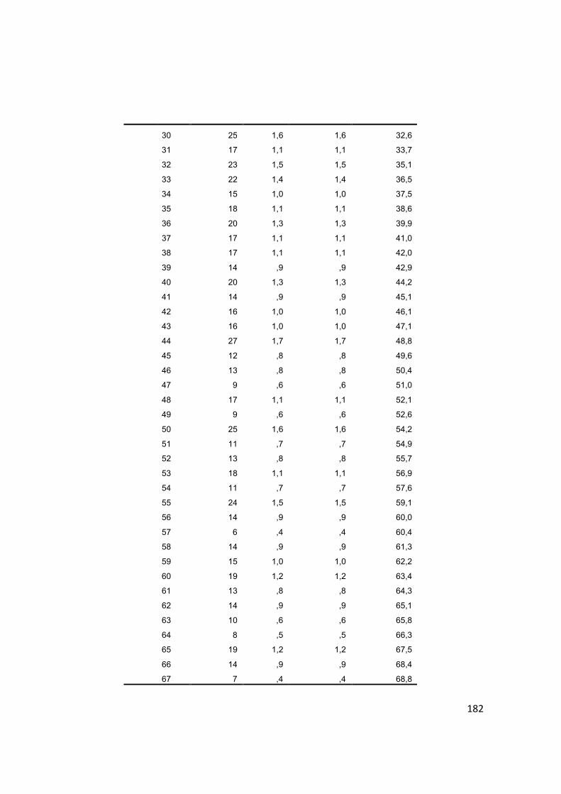
182

30 25 1,6 1,6 32,6

31 17 1,1 1,1 33,7

32 23 1,5 1,5 35,1

33 22 1,4 1,4 36,5

34 15 1,0 1,0 37,5

35 18 1,1 1,1 38,6

36 20 1,3 1,3 39,9

37 17 1,1 1,1 41,0

38 17 1,1 1,1 42,0

39 14 ,9 ,9 42,9

40 20 1,3 1,3 44,2

41 14 ,9 ,9 45,1

42 16 1,0 1,0 46,1

43 16 1,0 1,0 47,1

44 27 1,7 1,7 48,8

45 12 ,8 ,8 49,6

46 13 ,8 ,8 50,4

47 9 ,6 ,6 51,0

48 17 1,1 1,1 52,1

49 9 ,6 ,6 52,6

50 25 1,6 1,6 54,2

51 11 ,7 ,7 54,9

52 13 ,8 ,8 55,7

53 18 1,1 1,1 56,9

54 11 ,7 ,7 57,6

55 24 1,5 1,5 59,1

56 14 ,9 ,9 60,0

57 6 ,4 ,4 60,4

58 14 ,9 ,9 61,3

59 15 1,0 1,0 62,2

60 19 1,2 1,2 63,4

61 13 ,8 ,8 64,3

62 14 ,9 ,9 65,1

63 10 ,6 ,6 65,8

64 8 ,5 ,5 66,3

65 19 1,2 1,2 67,5

66 14 ,9 ,9 68,4

67 7 ,4 ,4 68,8

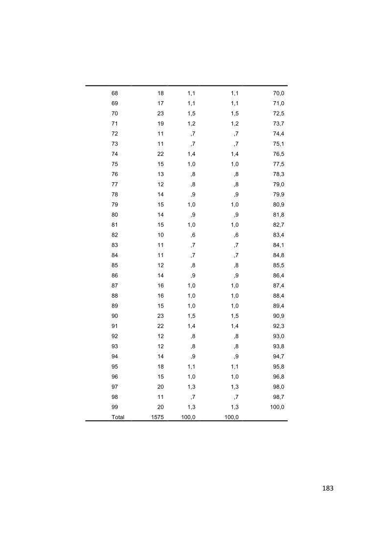
183

68 18 1,1 1,1 70,0

69 17 1,1 1,1 71,0

70 23 1,5 1,5 72,5

71 19 1,2 1,2 73,7

72 11 ,7 ,7 74,4

73 11 ,7 ,7 75,1

74 22 1,4 1,4 76,5

75 15 1,0 1,0 77,5

76 13 ,8 ,8 78,3

77 12 ,8 ,8 79,0

78 14 ,9 ,9 79,9

79 15 1,0 1,0 80,9

80 14 ,9 ,9 81,8

81 15 1,0 1,0 82,7

82 10 ,6 ,6 83,4

83 11 ,7 ,7 84,1

84 11 ,7 ,7 84,8

85 12 ,8 ,8 85,5

86 14 ,9 ,9 86,4

87 16 1,0 1,0 87,4

88 16 1,0 1,0 88,4

89 15 1,0 1,0 89,4

90 23 1,5 1,5 90,9

91 22 1,4 1,4 92,3

92 12 ,8 ,8 93,0

93 12 ,8 ,8 93,8

94 14 ,9 ,9 94,7

95 18 1,1 1,1 95,8

96 15 1,0 1,0 96,8

97 20 1,3 1,3 98,0

98 11 ,7 ,7 98,7

99 20 1,3 1,3 100,0

Total 1575 100,0 100,0

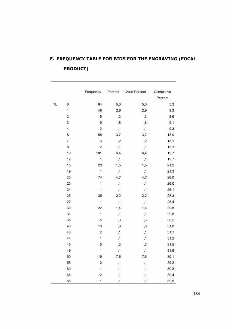
184

E. FREQUENCY TABLE FOR BIDS FOR THE ENGRAVING (FOCAL

PRODUCT)

Frequency Percent Valid Percent Cumulative

Percent

TL 0 84 5,3 5,3 5,3

1 46 2,9 2,9 8,3

2 5 ,3 ,3 8,6

3 9 ,6 ,6 9,1

4 2 ,1 ,1 9,3

5 58 3,7 3,7 13,0

7 3 ,2 ,2 13,1

8 2 ,1 ,1 13,3

10 101 6,4 6,4 19,7

12 1 ,1 ,1 19,7

15 23 1,5 1,5 21,2

19 1 ,1 ,1 21,3

20 74 4,7 4,7 26,0

23 1 ,1 ,1 26,0

24 1 ,1 ,1 26,1

25 35 2,2 2,2 28,3

27 1 ,1 ,1 28,4

30 22 1,4 1,4 29,8

31 1 ,1 ,1 29,8

35 5 ,3 ,3 30,2

40 13 ,8 ,8 31,0

43 2 ,1 ,1 31,1

44 1 ,1 ,1 31,2

45 5 ,3 ,3 31,5

49 1 ,1 ,1 31,6

50 119 7,6 7,6 39,1

55 2 ,1 ,1 39,2

60 1 ,1 ,1 39,3

65 2 ,1 ,1 39,4

68 1 ,1 ,1 39,5

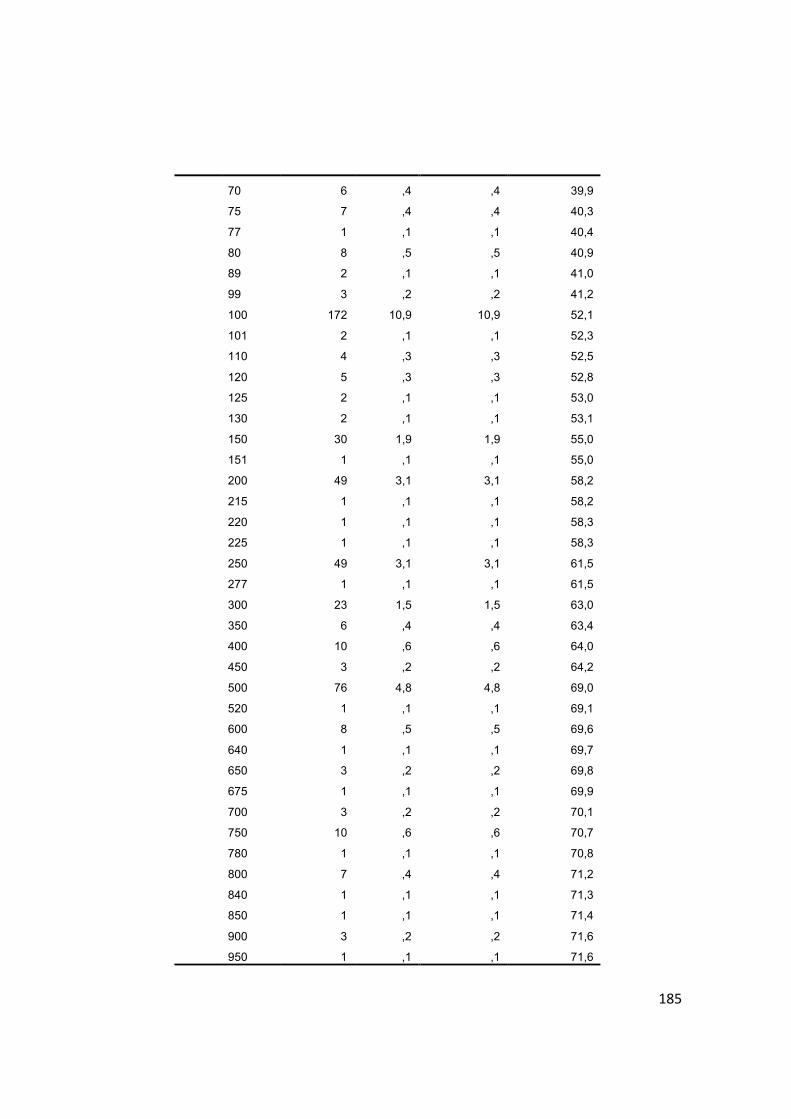
185

70 6 ,4 ,4 39,9

75 7 ,4 ,4 40,3

77 1 ,1 ,1 40,4

80 8 ,5 ,5 40,9

89 2 ,1 ,1 41,0

99 3 ,2 ,2 41,2

100 172 10,9 10,9 52,1

101 2 ,1 ,1 52,3

110 4 ,3 ,3 52,5

120 5 ,3 ,3 52,8

125 2 ,1 ,1 53,0

130 2 ,1 ,1 53,1

150 30 1,9 1,9 55,0

151 1 ,1 ,1 55,0

200 49 3,1 3,1 58,2

215 1 ,1 ,1 58,2

220 1 ,1 ,1 58,3

225 1 ,1 ,1 58,3

250 49 3,1 3,1 61,5

277 1 ,1 ,1 61,5

300 23 1,5 1,5 63,0

350 6 ,4 ,4 63,4

400 10 ,6 ,6 64,0

450 3 ,2 ,2 64,2

500 76 4,8 4,8 69,0

520 1 ,1 ,1 69,1

600 8 ,5 ,5 69,6

640 1 ,1 ,1 69,7

650 3 ,2 ,2 69,8

675 1 ,1 ,1 69,9

700 3 ,2 ,2 70,1

750 10 ,6 ,6 70,7

780 1 ,1 ,1 70,8

800 7 ,4 ,4 71,2

840 1 ,1 ,1 71,3

850 1 ,1 ,1 71,4

900 3 ,2 ,2 71,6

950 1 ,1 ,1 71,6

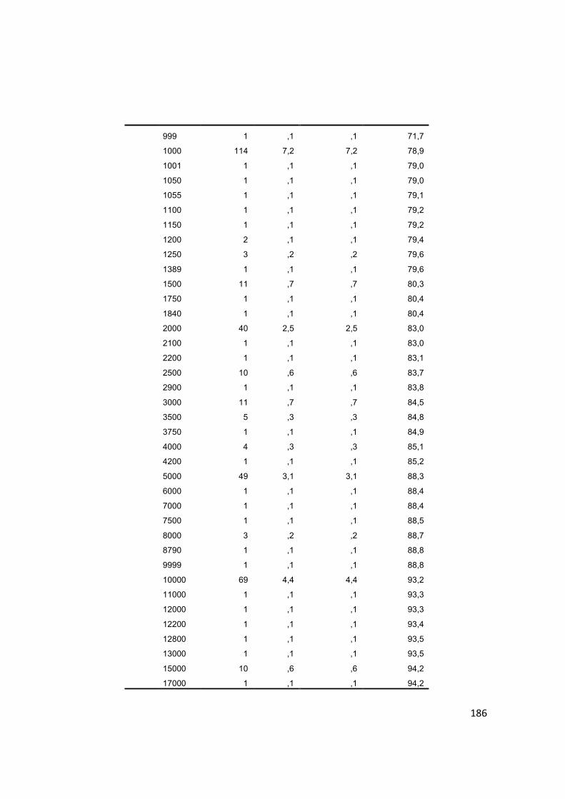
186

999 1 ,1 ,1 71,7

1000 114 7,2 7,2 78,9

1001 1 ,1 ,1 79,0

1050 1 ,1 ,1 79,0

1055 1 ,1 ,1 79,1

1100 1 ,1 ,1 79,2

1150 1 ,1 ,1 79,2

1200 2 ,1 ,1 79,4

1250 3 ,2 ,2 79,6

1389 1 ,1 ,1 79,6

1500 11 ,7 ,7 80,3

1750 1 ,1 ,1 80,4

1840 1 ,1 ,1 80,4

2000 40 2,5 2,5 83,0

2100 1 ,1 ,1 83,0

2200 1 ,1 ,1 83,1

2500 10 ,6 ,6 83,7

2900 1 ,1 ,1 83,8

3000 11 ,7 ,7 84,5

3500 5 ,3 ,3 84,8

3750 1 ,1 ,1 84,9

4000 4 ,3 ,3 85,1

4200 1 ,1 ,1 85,2

5000 49 3,1 3,1 88,3

6000 1 ,1 ,1 88,4

7000 1 ,1 ,1 88,4

7500 1 ,1 ,1 88,5

8000 3 ,2 ,2 88,7

8790 1 ,1 ,1 88,8

9999 1 ,1 ,1 88,8

10000 69 4,4 4,4 93,2

11000 1 ,1 ,1 93,3

12000 1 ,1 ,1 93,3

12200 1 ,1 ,1 93,4

12800 1 ,1 ,1 93,5

13000 1 ,1 ,1 93,5

15000 10 ,6 ,6 94,2

17000 1 ,1 ,1 94,2

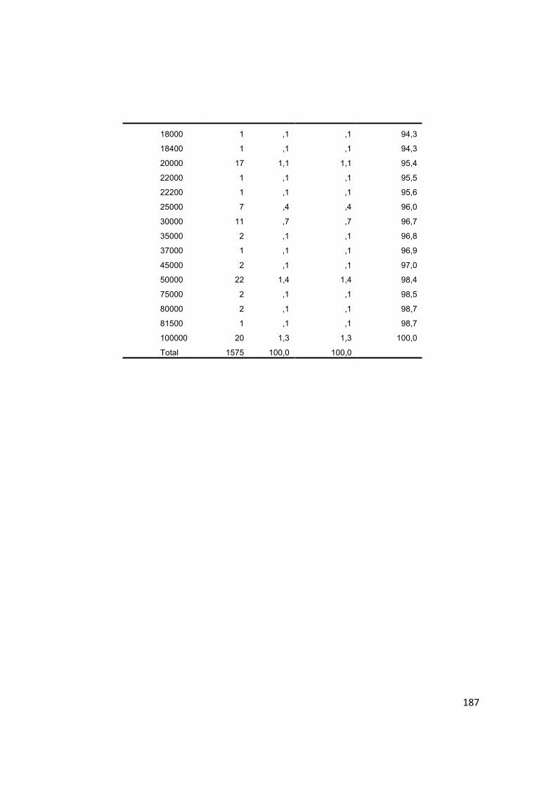
187

18000 1 ,1 ,1 94,3

18400 1 ,1 ,1 94,3

20000 17 1,1 1,1 95,4

22000 1 ,1 ,1 95,5

22200 1 ,1 ,1 95,6

25000 7 ,4 ,4 96,0

30000 11 ,7 ,7 96,7

35000 2 ,1 ,1 96,8

37000 1 ,1 ,1 96,9

45000 2 ,1 ,1 97,0

50000 22 1,4 1,4 98,4

75000 2 ,1 ,1 98,5

80000 2 ,1 ,1 98,7

81500 1 ,1 ,1 98,7

100000 20 1,3 1,3 100,0

Total 1575 100,0 100,0

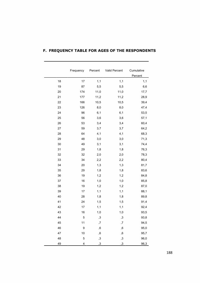
188

F. FREQUENCY TABLE FOR AGES OF THE RESPONDENTS

Frequency Percent Valid Percent Cumulative

Percent

18 17 1,1 1,1 1,1

19 87 5,5 5,5 6,6

20 174 11,0 11,0 17,7

21 177 11,2 11,2 28,9

22 166 10,5 10,5 39,4

23 126 8,0 8,0 47,4

24 96 6,1 6,1 53,5

25 56 3,6 3,6 57,1

26 53 3,4 3,4 60,4

27 59 3,7 3,7 64,2

28 64 4,1 4,1 68,3

29 48 3,0 3,0 71,3

30 49 3,1 3,1 74,4

31 29 1,8 1,8 76,3

32 32 2,0 2,0 78,3

33 34 2,2 2,2 80,4

34 20 1,3 1,3 81,7

35 29 1,8 1,8 83,6

36 19 1,2 1,2 84,8

37 16 1,0 1,0 85,8

38 19 1,2 1,2 87,0

39 17 1,1 1,1 88,1

40 28 1,8 1,8 89,8

41 24 1,5 1,5 91,4

42 17 1,1 1,1 92,4

43 16 1,0 1,0 93,5

44 5 ,3 ,3 93,8

45 11 ,7 ,7 94,5

46 9 ,6 ,6 95,0

47 10 ,6 ,6 95,7

48 5 ,3 ,3 96,0

49 4 ,3 ,3 96,3

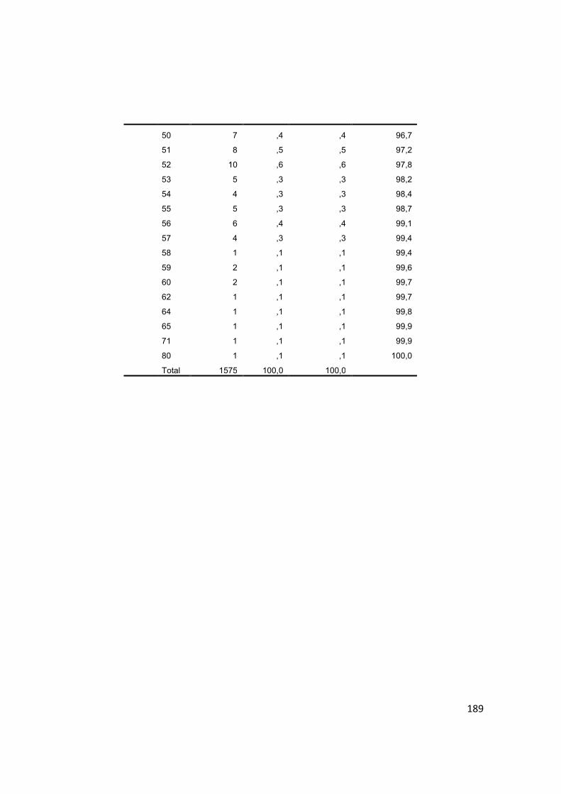
189

50 7 ,4 ,4 96,7

51 8 ,5 ,5 97,2

52 10 ,6 ,6 97,8

53 5 ,3 ,3 98,2

54 4 ,3 ,3 98,4

55 5 ,3 ,3 98,7

56 6 ,4 ,4 99,1

57 4 ,3 ,3 99,4

58 1 ,1 ,1 99,4

59 2 ,1 ,1 99,6

60 2 ,1 ,1 99,7

62 1 ,1 ,1 99,7

64 1 ,1 ,1 99,8

65 1 ,1 ,1 99,9

71 1 ,1 ,1 99,9

80 1 ,1 ,1 100,0

Total 1575 100,0 100,0

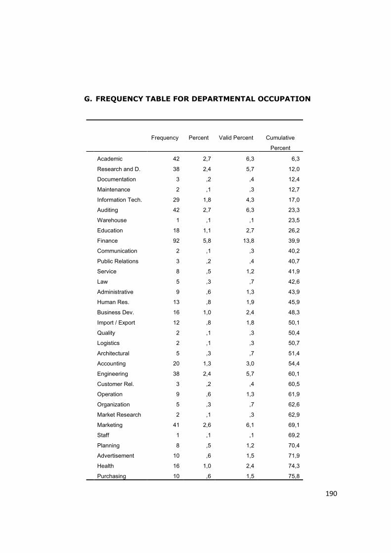
190

G. FREQUENCY TABLE FOR DEPARTMENTAL OCCUPATION

Frequency Percent Valid Percent Cumulative

Percent

Academic 42 2,7 6,3 6,3

Research and D. 38 2,4 5,7 12,0

Documentation 3 ,2 ,4 12,4

Maintenance 2 ,1 ,3 12,7

Information Tech. 29 1,8 4,3 17,0

Auditing 42 2,7 6,3 23,3

Warehouse 1 ,1 ,1 23,5

Education 18 1,1 2,7 26,2

Finance 92 5,8 13,8 39,9

Communication 2 ,1 ,3 40,2

Public Relations 3 ,2 ,4 40,7

Service 8 ,5 1,2 41,9

Law 5 ,3 ,7 42,6

Administrative 9 ,6 1,3 43,9

Human Res. 13 ,8 1,9 45,9

Business Dev. 16 1,0 2,4 48,3

Import / Export 12 ,8 1,8 50,1

Quality 2 ,1 ,3 50,4

Logistics 2 ,1 ,3 50,7

Architectural 5 ,3 ,7 51,4

Accounting 20 1,3 3,0 54,4

Engineering 38 2,4 5,7 60,1

Customer Rel. 3 ,2 ,4 60,5

Operation 9 ,6 1,3 61,9

Organization 5 ,3 ,7 62,6

Market Research 2 ,1 ,3 62,9

Marketing 41 2,6 6,1 69,1

Staff 1 ,1 ,1 69,2

Planning 8 ,5 1,2 70,4

Advertisement 10 ,6 1,5 71,9

Health 16 1,0 2,4 74,3

Purchasing 10 ,6 1,5 75,8

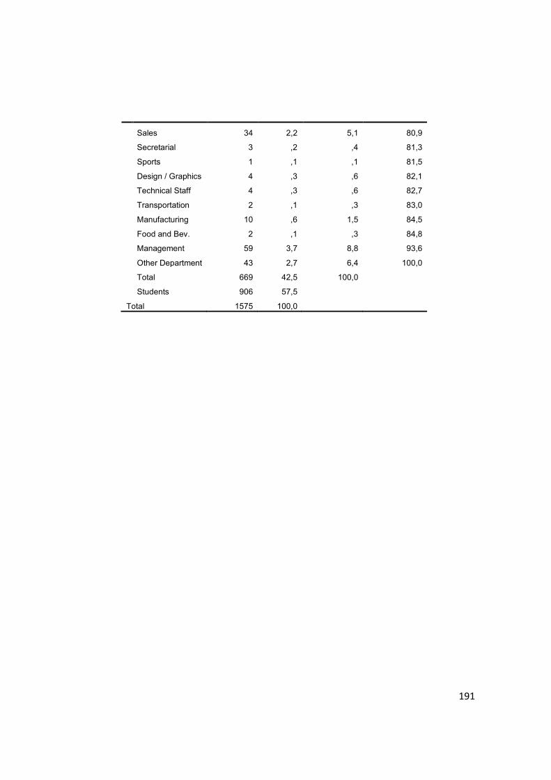
191

Sales 34 2,2 5,1 80,9

Secretarial 3 ,2 ,4 81,3

Sports 1 ,1 ,1 81,5

Design / Graphics 4 ,3 ,6 82,1

Technical Staff 4 ,3 ,6 82,7

Transportation 2 ,1 ,3 83,0

Manufacturing 10 ,6 1,5 84,5

Food and Bev. 2 ,1 ,3 84,8

Management 59 3,7 8,8 93,6

Other Department 43 2,7 6,4 100,0

Total 669 42,5 100,0

Students 906 57,5

Total 1575 100,0

192

H. OFFICIAL PERMISSION LETTER OF METU ETHICAL

COMMITTEE