Inverted Pendulum Demonstration

Candidate Number: 8240R

Supervisor: Dr. Christopher Lester

The unstable point above a pendulum’s centre of mass can be made stable by

rapidly oscillating the support. This report will use this ‘Dynamic Stability’ condi-

tion to design and build an accurate and robust demonstration of the phenomenon,

by using a jigsaw. Dynamic stability has important implications for any system that

benefits from forced stability, from particle traps to high temperature superconduc-

tivity. The theory of dynamic stability is investigated and the state of research is

summarised, with a review into previous designs used to justify our chosen design. A

numerical integrator with an adaptive step is written and shown to accurately pre-

dict the pendulum dynamics. The frictional form of the pendulum is found to vary

with the angular speed, by measuring the amplitude decay with a high speed camera.

Subsequently, the exact frictional co-e�cient of the pendulum is calculated and input

into the model. Finally, the jigsaw is shown to exhibit inverted pendulum dynamics,

and the minimum threshold frequency is measured for 5 di↵erent lengths. The data is

revealed to be in good agreement with both the theoretical values and the computer

model, and a relationship was found between the minimum frequency and the initial

displacement.

1 Introduction

For over 300 years, Galileo’s pendulum study hasbeen one of the axioms of classical dynamics inmechanical systems.1 However, a peculiar phe-nomenon occurs when the suspension point isvertically oscillated. The unstable point abovethe centre of gravity becomes dynamically sta-bilised, and can be shown to oscillate aboutthis new stable position. Although extremelycounter-intuitive, dynamic stabilisation is muchmore obvious in a gyroscopic-top or a man on aunicycle, both of which find stability by assum-ing the most vertical position.

Dynamic stability was first investigated byStephenson in 1908, who found that stability canbe incurred by periodic oscillations and appliedto a pendulum with a rapidly vibrating support.2

Kapitza further investigated the stability condi-tions and solved the arising Mathieu equation,

before using successive approximations to solvethe problem outside of the small angle approx-imation.3 In addition, Kapitza experimentallyinvestigated the conditions, building a ‘KapitzaPendulum’, which used a rotary-to-linear devicefrom a sewing machine to vertically drive a pen-dulum.4 In 1985, Michaelis created an inexpen-sive demonstration of the phenomenon using ahandheld jigsaw, and in 1992, the limits of thestability of the system were experimentally stud-ied by fashioning an oscillator out of speaker-coils.5–7 There have been numerous attempts atelaborating on the mathematics, by both consid-ering sinusoidal oscillations, and non-parametricsaw tooth oscillations which simplify the math-ematics.8–10 A large number of systems haveequations of motion analogous to the Mathieuequation, and so can undergo dynamic stability.These include: particles in a cyclotron, levitatingliquid droplets and confined charged particles in

1

a Paul trap.11–13 Furthermore, there has beenrecent interest in the use of dynamic stability tocreate super-conducting states at room temper-ature.14

Although previous work has concentrated onthe mathematics and stability conditions, herewe will rigorously create a robust experimen-tal demonstration of the inverted pendulum thatgives accurate measurements, and can be used todisplay dynamic stabilisation to large audiences.Furthermore, a computer model will be createdin tandem with the physical apparatus, and willbe used to model the dynamics in the absence ofmechanical vibrations or resonances.

The report will begin by summarising thetheory of dynamic stabilisation, before numer-ically integrating the equation of motion in acomputer model. Previous designs in the liter-ature will be reviewed to help create our owninverted pendulum demonstration, and each fea-ture will be justified. The friction of the pendu-lum will be determined, before the final modelis used to compare the minimum frequency ofoscillation with the theory.

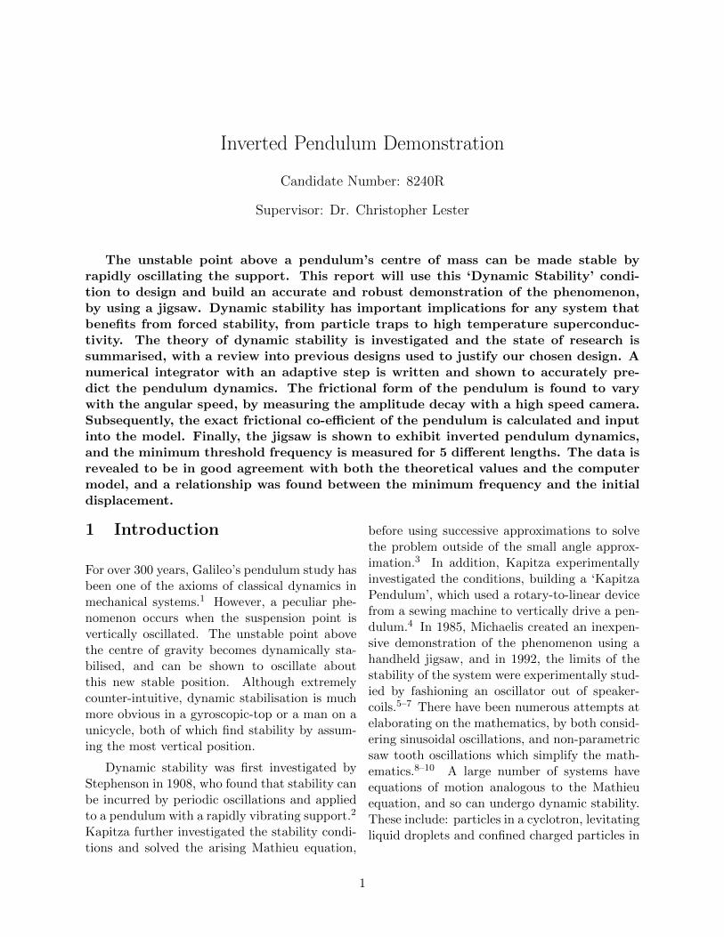
Figure 1: Force diagram of the pendulum perpendicu-lar to the oscillations, and at an arbitrary angle .15

2 Background Theory

2.1 Dynamic Stabilisation

Physically, we can understand dynamic stabil-ity by considering the torques acting. Neglect-ing gravity, if there is zero initial velocity andthe rod is displaced perpendicular to the oscilla-

tions, in the inertial frame of the pivot the centreof masses (COM) are placed on a circular arc,as shown in figure 1a, with equal and oppositetorques.

If the rod is at an arbitrary angle abovethe horizontal, the forces are still the same, butthe length of the moment is longer for position2, as seen in figure 1b. If the angle was belowthe horizontal the converse would be true.

Thus, on average there is a greater restor-ing torque towards the upward vertical. In thepresence of gravity, stability is achieved if thisvibrational torque, averaged over many cycles,is greater than the gravitational torque.15

Consider a rigid pendulum of length l, massm, and COM ↵l, with moment of inertia ICOM .

The pendulum’s support is vertically dis-placed by a sinusoidal oscillation with drivingfrequency ⌦ and amplitude A: a(t) = A cos⌦t.At an angle ✓ from the upper vertical, the COMhas x and y coordinates, x = ↵l sin ✓ and y =↵l cos ✓ + a(t).

To derive the equation of motion we use La-grangian mechanics.

As derived in the appendix(A.1), the La-grangian in full is:

L =1

2m⇥(↵l✓)2+ a2+2a↵l✓ sin ✓

⇤+

1

2ICOM ✓

2

�mg(↵l cos ✓ + a(t)) (1)

The Euler-Lagrange equation (2) can be usedto derive the equation of motion:

d

dt

⇣�L�✓

⌘� �L

�✓= F✓ (2)

where the Dissipative Force F✓ will be elaboratedupon in section 2.2.

Assuming F✓ = 0, solving (2) using (1) yieldsthe equation of motion:

✓ +↵

↵2 + �(↵)

⇣⌦2A

lcos⌦t� g

l

⌘sin ✓ = 0 (3)

where �(↵) = ICOMml2

as shown in A.1. This is aform of the Mathieu equation.

This motion is of similar form to a simplependulum, with the acceleration due to gravity

2

modulated by a vertical driving force. As thisform is analogous to a simple harmonic oscillator(✓+!2✓ = 0), the period can be easily calculatedfrom T = 2⇡/!.

Ignoring friction, we can derive the conditionfor dynamic stabilisation by writing ✓ in termsof slowly varying variables: ✓1, C, and S:

✓ = ✓1 + C cos⌦t+ S sin⌦t (4)

This allows us to write the equation of mo-tion in terms of ✓1, assuming ⌦2 � g

l , which iseasily achievable with a powerful oscillator.

After some manipulation(see A.2), we findfor small ✓1:

✓1+↵

↵2 + �(↵)

✓⌦2A2↵

2l2(↵2 + �(↵))� g

l

◆✓1 = 0 (5)

The upright position is only stable if thereis a restoring force in the direction of the up-per vertical, thus the term in brackets must bepositive.

The condition for stability is:

⌦2 >2(↵2 + �(↵))gl

↵A2(6)

This condition is important as it gives us thecritical frequency, ⌦c, in which the constructedinverted pendulum will work; although we haveneglected friction which may be important in thephysical model. Later on, ⌦c will be investigatedfurther, and used as a guideline for the parame-ters of our inverted pendulum.

2.2 Dissipative Friction

In any sort of physical system there will be fric-tional forces acting. The dissipative force is pro-portional to the velocity of the system, v, raisedto some power n, and opposes motion:

F = �sign(v)n+1�vn = �sign(✓)n+1�(↵l✓)n

(7)where � is a constant, and the sign function

ensures that the friction opposes motion.If n = 0, the friction is directly proportional

to the contact force and independent of speedor area, and is known as dry friction. Viscousfriction, given by n = 1, increases linearly withv. High velocity friction, n = 2, tends to dom-inate when the speed v is very large, or in highReynolds number regimes.16

In an ideal pendulum system, the frictionterm is proportional to ✓, however care will betaken in this investigation to measure n.17 Thefinal dissipation function18 is derived in A.3, andF✓ is found to be:

F✓ = �sign(✓)n+1�(✓)n (8)

In section 5, the friction will be investigatedto find n.

3 Computational Method

3.1 Adaptive Step Runge-Kutta

Method

Although (3) can be solved analytically using theMathieu equation, here the Runge-Kutta (RK)method with an adaptive step will be used to in-tegrate the di↵erential equations numerically.19

The RK method performs a number of stepsat di↵erent points along the interval and finds aweighted average, which is dependent upon howclose the steps are to the midpoint.20

We will use the adaptive step Runge-Kutta-Fehlberg method, which removes the step sizedependence by including a procedure to see ifthe proper step-size, h, is being used.21 If weperform a step h1 with error e1, the optimal step-size h2 that gives an error equal to the tolerance✏ is:

h2 = 0.9h1⇣e(h1)

✏

⌘ 15

(9)

The extra 0.9 is added as a small margin of safetyfor any approximations made. If h2 � h1, thenh1 is accepted, otherwise the integration is re-peated with h2 (for full consideration see A.4).

The parameters inputted into the model arethe maximum tolerance and maximum time.The algorithm proceeds step by step until thistolerance is exceeded or the maximum time isreached.

3

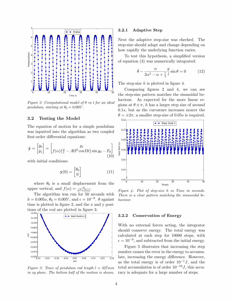
Figure 2: Computational model of ✓ vs t for an idealpendulum, starting at ✓0 = 0.005c.

3.2 Testing the Model

The equation of motion for a simple pendulumwas inputted into the algorithm as two coupledfirst-order di↵erential equations:

y =

y0y1

�=

y1

f(↵)�gl �A⌦2 cos⌦t

�sin y0 � F✓

�

(10)with initial conditions:

y(0) =

✓00

�(11)

where ✓0 is a small displacement from theupper vertical, and f(↵) = ↵

↵2+�(↵) .

The algorithm was run for 50 seconds withh = 0.005s, ✓0 = 0.005c, and ✏ = 10�9. ✓ againsttime is plotted in figure 2, and the x and y posi-tions of the rod are plotted in figure 3.

Figure 3: Trace of pendulum rod length l = 427mmin xy plane. The bottom half of the motion is shown.

3.2.1 Adaptive Step

Next the adaptive step-size was checked. Thestep-size should adapt and change depending onhow rapidly the underlying function varies.

To test this hypothesis, a simplified versionof equation (3) was numerically integrated:

✓ � ↵

2↵2 � ↵+ 13

g

lsin ✓ = 0 (12)

The step-size h is plotted in figure 4.

Comparing figures 2 and 4, we can seethe step-size pattern matches the sinusoidal be-haviour. As expected for the more linear re-gions at ✓± ⇡, h has a larger step size of around0.1s, but as the curvature increases nearer the✓ = ±2⇡, a smaller step-size of 0.05s is required.

Figure 4: Plot of step-size h vs Time in seconds.There is a clear pattern matching the sinusoidal be-haviour.

3.2.2 Conservation of Energy

With no external forces acting, the integratorshould conserve energy. The total energy wascalculated at each step for 10000 steps, with✏ = 10�9, and subtracted from the initial energy.

Figure 5 illustrates that increasing the stepnumber causes the error in the energy to accumu-late, increasing the energy di↵erence. However,as the total energy is of order 10�1J , and thetotal accumulation is of order 10�10J , this accu-racy is adequate for a large number of steps.

4

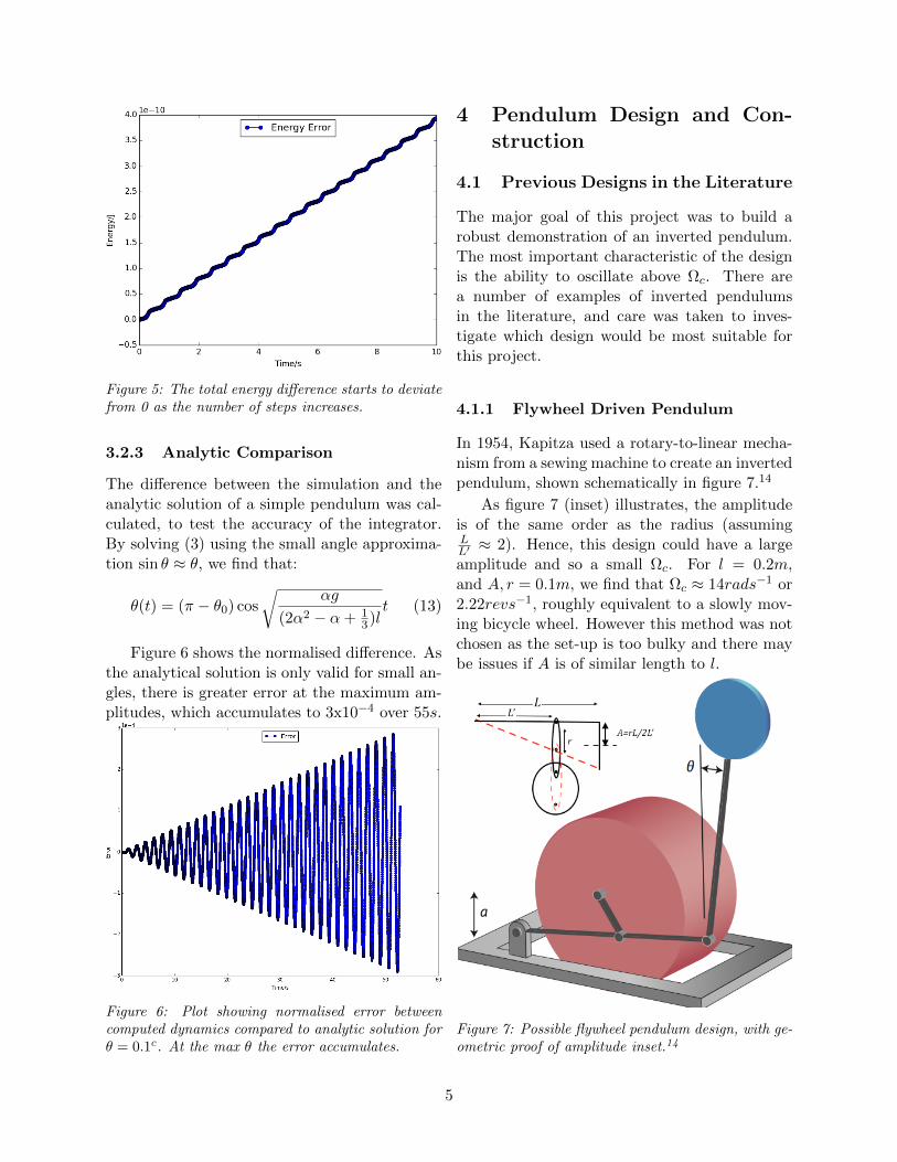
Figure 5: The total energy di↵erence starts to deviatefrom 0 as the number of steps increases.

3.2.3 Analytic Comparison

The di↵erence between the simulation and theanalytic solution of a simple pendulum was cal-culated, to test the accuracy of the integrator.By solving (3) using the small angle approxima-tion sin ✓ ⇡ ✓, we find that:

✓(t) = (⇡ � ✓0) cosr

↵g

(2↵2 � ↵+ 13)l

t (13)

Figure 6 shows the normalised di↵erence. Asthe analytical solution is only valid for small an-gles, there is greater error at the maximum am-plitudes, which accumulates to 3x10�4 over 55s.

Figure 6: Plot showing normalised error betweencomputed dynamics compared to analytic solution for✓ = 0.1c. At the max ✓ the error accumulates.

4 Pendulum Design and Con-

struction

4.1 Previous Designs in the Literature

The major goal of this project was to build arobust demonstration of an inverted pendulum.The most important characteristic of the designis the ability to oscillate above ⌦c. There area number of examples of inverted pendulumsin the literature, and care was taken to inves-tigate which design would be most suitable forthis project.

4.1.1 Flywheel Driven Pendulum

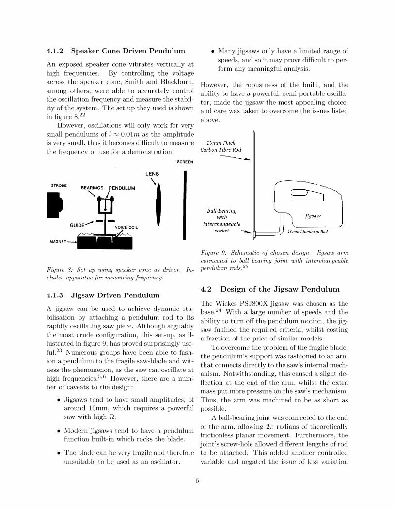
In 1954, Kapitza used a rotary-to-linear mecha-nism from a sewing machine to create an invertedpendulum, shown schematically in figure 7.14

As figure 7 (inset) illustrates, the amplitudeis of the same order as the radius (assumingLL0 ⇡ 2). Hence, this design could have a largeamplitude and so a small ⌦c. For l = 0.2m,and A, r = 0.1m, we find that ⌦c ⇡ 14rads�1 or2.22revs�1, roughly equivalent to a slowly mov-ing bicycle wheel. However this method was notchosen as the set-up is too bulky and there maybe issues if A is of similar length to l.

Figure 7: Possible flywheel pendulum design, with ge-ometric proof of amplitude inset.14

5

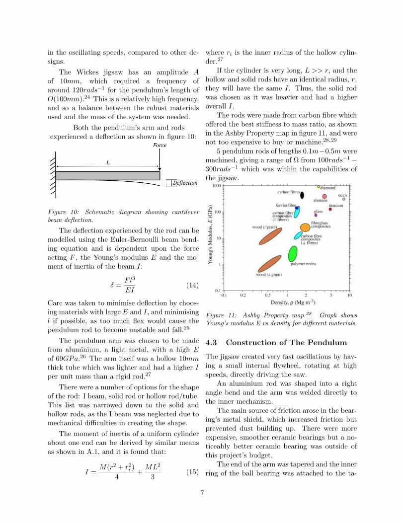
4.1.2 Speaker Cone Driven Pendulum

An exposed speaker cone vibrates vertically athigh frequencies. By controlling the voltageacross the speaker cone, Smith and Blackburn,among others, were able to accurately controlthe oscillation frequency and measure the stabil-ity of the system. The set up they used is shownin figure 8.22

However, oscillations will only work for verysmall pendulums of l ⇡ 0.01m as the amplitudeis very small, thus it becomes di�cult to measurethe frequency or use for a demonstration.

Figure 8: Set up using speaker cone as driver. In-cludes apparatus for measuring frequency.

4.1.3 Jigsaw Driven Pendulum

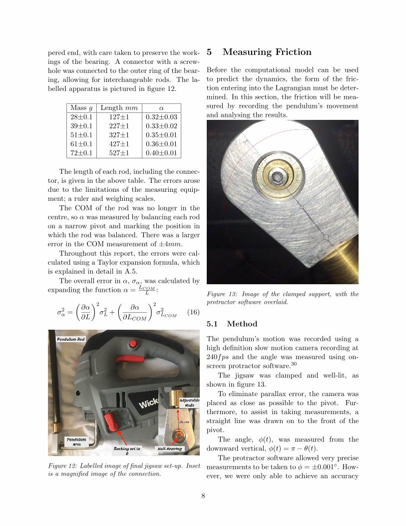
A jigsaw can be used to achieve dynamic sta-bilisation by attaching a pendulum rod to itsrapidly oscillating saw piece. Although arguablythe most crude configuration, this set-up, as il-lustrated in figure 9, has proved surprisingly use-ful.23 Numerous groups have been able to fash-ion a pendulum to the fragile saw-blade and wit-ness the phenomenon, as the saw can oscillate athigh frequencies.5,6 However, there are a num-ber of caveats to the design:

• Jigsaws tend to have small amplitudes, ofaround 10mm, which requires a powerfulsaw with high ⌦.

• Modern jigsaws tend to have a pendulumfunction built-in which rocks the blade.

• The blade can be very fragile and thereforeunsuitable to be used as an oscillator.

• Many jigsaws only have a limited range ofspeeds, and so it may prove di�cult to per-form any meaningful analysis.

However, the robustness of the build, and theability to have a powerful, semi-portable oscilla-tor, made the jigsaw the most appealing choice,and care was taken to overcome the issues listedabove.

Figure 9: Schematic of chosen design. Jigsaw armconnected to ball bearing joint with interchangeablependulum rods.23

4.2 Design of the Jigsaw Pendulum

The Wickes PSJ800X jigsaw was chosen as thebase.24 With a large number of speeds and theability to turn o↵ the pendulum motion, the jig-saw fulfilled the required criteria, whilst costinga fraction of the price of similar models.

To overcome the problem of the fragile blade,the pendulum’s support was fashioned to an armthat connects directly to the saw’s internal mech-anism. Notwithstanding, this caused a slight de-flection at the end of the arm, whilst the extramass put more pressure on the saw’s mechanism.Thus, the arm was machined to be as short aspossible.

A ball-bearing joint was connected to the endof the arm, allowing 2⇡ radians of theoreticallyfrictionless planar movement. Furthermore, thejoint’s screw-hole allowed di↵erent lengths of rodto be attached. This added another controlledvariable and negated the issue of less variation

6

in the oscillating speeds, compared to other de-signs.

The Wickes jigsaw has an amplitude Aof 10mm, which required a frequency ofaround 120rads�1 for the pendulum’s length ofO(100mm).24 This is a relatively high frequency,and so a balance between the robust materialsused and the mass of the system was needed.

Both the pendulum’s arm and rodsexperienced a deflection as shown in figure 10:

Figure 10: Schematic diagram showing cantileverbeam deflection.

The deflection experienced by the rod can bemodelled using the Euler-Bernoulli beam bend-ing equation and is dependent upon the forceacting F , the Young’s modulus E and the mo-ment of inertia of the beam I:

� =Fl3

EI(14)

Care was taken to minimise deflection by choos-ing materials with large E and I, and minimisingl if possible, as too much flex would cause thependulum rod to become unstable and fall.25

The pendulum arm was chosen to be madefrom aluminium, a light metal, with a high Eof 69GPa.26 The arm itself was a hollow 10mmthick tube which was lighter and had a higher Iper unit mass than a rigid rod.27

There were a number of options for the shapeof the rod: I beam, solid rod or hollow rod/tube.This list was narrowed down to the solid andhollow rods, as the I beam was neglected due tomechanical di�culties in creating the shape.

The moment of inertia of a uniform cylinderabout one end can be derived by similar meansas shown in A.1, and it is found that:

I =M(r2 + r2i )

4+

ML2

3(15)

where ri is the inner radius of the hollow cylin-der.27

If the cylinder is very long, L >> r, and thehollow and solid rods have an identical radius, r,they will have the same I. Thus, the solid rodwas chosen as it was heavier and had a higheroverall I.

The rods were made from carbon fibre whicho↵ered the best sti↵ness to mass ratio, as shownin the Ashby Property map in figure 11, and werenot too expensive to buy or machine.28,29

5 pendulum rods of lengths 0.1m�0.5m weremachined, giving a range of ⌦ from 100rads�1�300rads�1 which was within the capabilities ofthe jigsaw.

Figure 11: Ashby Property map.28 Graph showsYoung’s modulus E vs density for di↵erent materials.

4.3 Construction of The Pendulum

The jigsaw created very fast oscillations by hav-ing a small internal flywheel, rotating at highspeeds, directly driving the saw.

An aluminium rod was shaped into a rightangle bend and the arm was welded directly tothe inner mechanism.

The main source of friction arose in the bear-ing’s metal shield, which increased friction butprevented dust building up. There were moreexpensive, smoother ceramic bearings but a no-ticeably better ceramic bearing was outside ofthis project’s budget.

The end of the arm was tapered and the innerring of the ball bearing was attached to the ta-

7

pered end, with care taken to preserve the work-ings of the bearing. A connector with a screw-hole was connected to the outer ring of the bear-ing, allowing for interchangeable rods. The la-belled apparatus is pictured in figure 12.

Mass g Length mm ↵

28±0.1 127±1 0.32±0.0339±0.1 227±1 0.33±0.0251±0.1 327±1 0.35±0.0161±0.1 427±1 0.36±0.0172±0.1 527±1 0.40±0.01

The length of each rod, including the connec-tor, is given in the above table. The errors arosedue to the limitations of the measuring equip-ment; a ruler and weighing scales.

The COM of the rod was no longer in thecentre, so ↵ was measured by balancing each rodon a narrow pivot and marking the position inwhich the rod was balanced. There was a largererror in the COM measurement of ±4mm.

Throughout this report, the errors were cal-culated using a Taylor expansion formula, whichis explained in detail in A.5.

The overall error in ↵, �↵, was calculated byexpanding the function ↵ = LCOM

L :

�2↵ =

✓@↵

@L

◆2

�2L +

✓@↵

@LCOM

◆2

�2LCOM(16)

Figure 12: Labelled image of final jigsaw set-up. Insetis a magnified image of the connection.

5 Measuring Friction

Before the computational model can be usedto predict the dynamics, the form of the fric-tion entering into the Lagrangian must be deter-mined. In this section, the friction will be mea-sured by recording the pendulum’s movementand analysing the results.

Figure 13: Image of the clamped support, with theprotractor software overlaid.

5.1 Method

The pendulum’s motion was recorded using ahigh definition slow motion camera recording at240fps and the angle was measured using on-screen protractor software.30

The jigsaw was clamped and well-lit, asshown in figure 13.

To eliminate parallax error, the camera wasplaced as close as possible to the pivot. Fur-thermore, to assist in taking measurements, astraight line was drawn on to the front of thepivot.

The angle, �(t), was measured from thedownward vertical, �(t) = ⇡ � ✓(t).

The protractor software allowed very precisemeasurements to be taken to � = ±0.001�. How-ever, we were only able to achieve an accuracy

8

of ±1� due to the finite resolution of the video.The software also measured the angle from

an arbitrary vertical on-screen. Thus the read-ings were adjusted using the ‘zero-point’ valueof �, which is the value of � on-screen when thependulum was actually at � = 0�.

Although the accuracy of the video is 240fps,there was some sampling error, as it was di�-cult to judge the point of maximum amplitude.To help our observations, the time was also ad-justed so t0 = 0s ,which gave an overall error inthe time of ±0.05s.

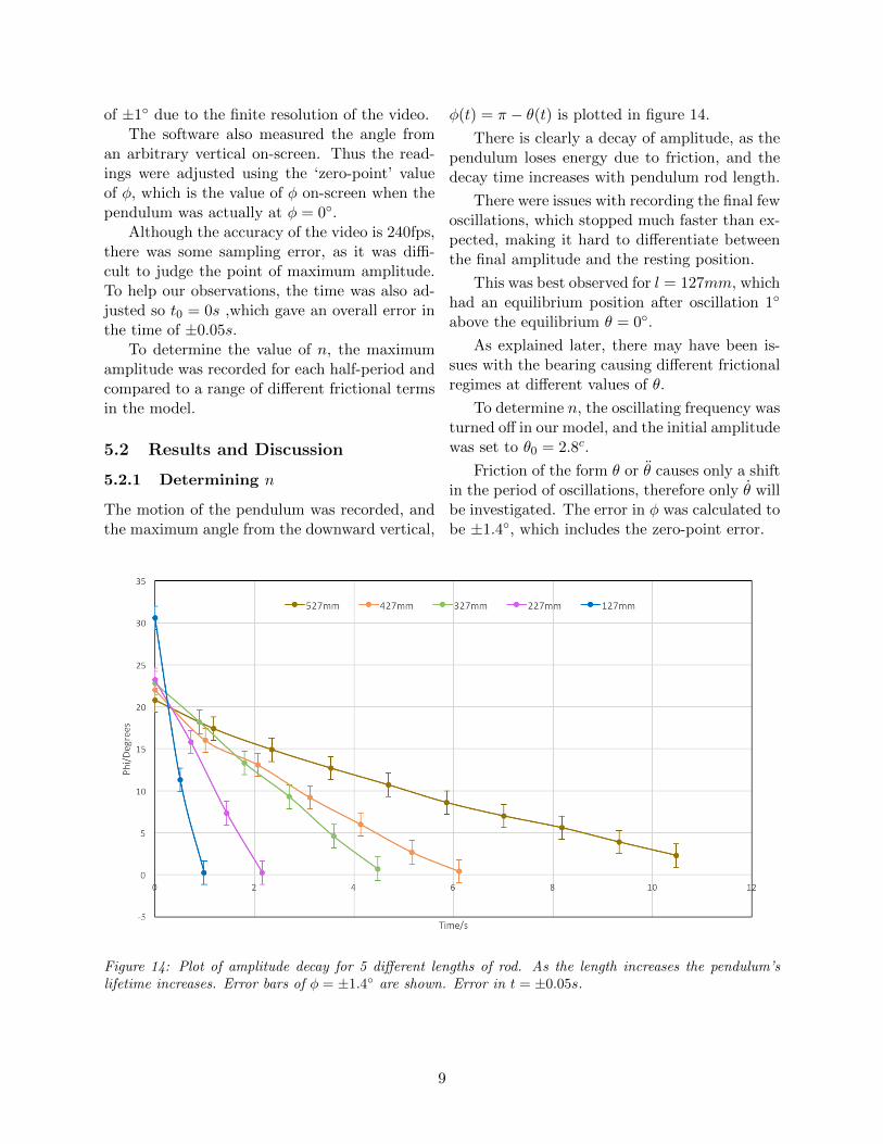
To determine the value of n, the maximumamplitude was recorded for each half-period andcompared to a range of di↵erent frictional termsin the model.

5.2 Results and Discussion

5.2.1 Determining n

The motion of the pendulum was recorded, andthe maximum angle from the downward vertical,

�(t) = ⇡ � ✓(t) is plotted in figure 14.

There is clearly a decay of amplitude, as thependulum loses energy due to friction, and thedecay time increases with pendulum rod length.

There were issues with recording the final fewoscillations, which stopped much faster than ex-pected, making it hard to di↵erentiate betweenthe final amplitude and the resting position.

This was best observed for l = 127mm, whichhad an equilibrium position after oscillation 1�

above the equilibrium ✓ = 0�.

As explained later, there may have been is-sues with the bearing causing di↵erent frictionalregimes at di↵erent values of ✓.

To determine n, the oscillating frequency wasturned o↵ in our model, and the initial amplitudewas set to ✓0 = 2.8c.

Friction of the form ✓ or ✓ causes only a shiftin the period of oscillations, therefore only ✓ willbe investigated. The error in � was calculated tobe ±1.4�, which includes the zero-point error.

Figure 14: Plot of amplitude decay for 5 di↵erent lengths of rod. As the length increases the pendulum’slifetime increases. Error bars of � = ±1.4� are shown. Error in t = ±0.05s.

9

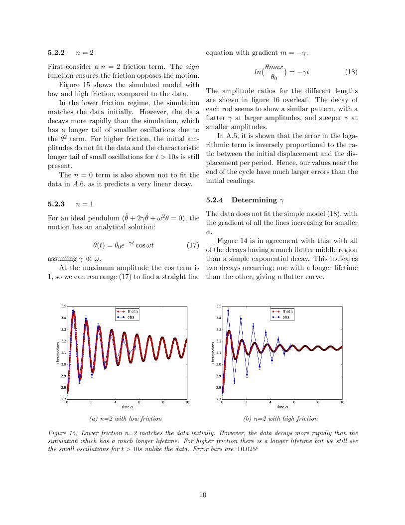
5.2.2 n = 2

First consider a n = 2 friction term. The signfunction ensures the friction opposes the motion.

Figure 15 shows the simulated model withlow and high friction, compared to the data.

In the lower friction regime, the simulationmatches the data initially. However, the datadecays more rapidly than the simulation, whichhas a longer tail of smaller oscillations due tothe ✓2 term. For higher friction, the initial am-plitudes do not fit the data and the characteristiclonger tail of small oscillations for t > 10s is stillpresent.

The n = 0 term is also shown not to fit thedata in A.6, as it predicts a very linear decay.

5.2.3 n = 1

For an ideal pendulum (✓ + 2�✓ + !2✓ = 0), themotion has an analytical solution:

✓(t) = ✓0e��t cos!t (17)

assuming � ⌧ !.At the maximum amplitude the cos term is

1, so we can rearrange (17) to find a straight line

equation with gradient m = ��:

ln�✓max

✓0

�= ��t (18)

The amplitude ratios for the di↵erent lengthsare shown in figure 16 overleaf. The decay ofeach rod seems to show a similar pattern, with aflatter � at larger amplitudes, and steeper � atsmaller amplitudes.

In A.5, it is shown that the error in the loga-rithmic term is inversely proportional to the ra-tio between the initial displacement and the dis-placement per period. Hence, our values near theend of the cycle have much larger errors than theinitial readings.

5.2.4 Determining �

The data does not fit the simple model (18), withthe gradient of all the lines increasing for smaller�.

Figure 14 is in agreement with this, with allof the decays having a much flatter middle regionthan a simple exponential decay. This indicatestwo decays occurring; one with a longer lifetimethan the other, giving a flatter curve.

(a) n=2 with low friction (b) n=2 with high friction

Figure 15: Lower friction n=2 matches the data initially. However, the data decays more rapidly than thesimulation which has a much longer lifetime. For higher friction there is a longer lifetime but we still seethe small oscillations for t > 10s unlike the data. Error bars are ±0.025c

10

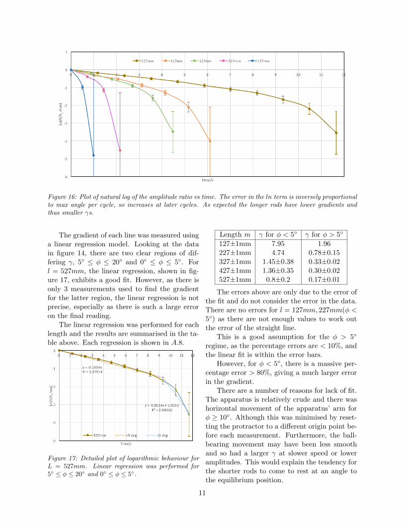
Figure 16: Plot of natural log of the amplitude ratio vs time. The error in the ln term is inversely proportionalto max angle per cycle, so increases at later cycles. As expected the longer rods have lower gradients andthus smaller �s.

The gradient of each line was measured usinga linear regression model. Looking at the datain figure 14, there are two clear regions of dif-fering �, 5� � 20� and 0� � 5�. Forl = 527mm, the linear regression, shown in fig-ure 17, exhibits a good fit. However, as there isonly 3 measurements used to find the gradientfor the latter region, the linear regression is notprecise, especially as there is such a large erroron the final reading.

The linear regression was performed for eachlength and the results are summarised in the ta-ble above. Each regression is shown in A.8.

Figure 17: Detailed plot of logarithmic behaviour forL = 527mm. Linear regression was performed for5� � 20� and 0� � 5�.

Length m � for � < 5� � for � > 5�

127±1mm 7.95 1.96227±1mm 4.74 0.78±0.15327±1mm 1.45±0.38 0.33±0.02427±1mm 1.36±0.35 0.30±0.02527±1mm 0.8±0.2 0.17±0.01

The errors above are only due to the error ofthe fit and do not consider the error in the data.There are no errors for l = 127mm, 227mm(� <5�) as there are not enough values to work outthe error of the straight line.

This is a good assumption for the � > 5�

regime, as the percentage errors are < 10%, andthe linear fit is within the error bars.

However, for � < 5�, there is a massive per-centage error > 80%, giving a much larger errorin the gradient.

There are a number of reasons for lack of fit.The apparatus is relatively crude and there washorizontal movement of the apparatus’ arm for� � 10�. Although this was minimised by reset-ting the protractor to a di↵erent origin point be-fore each measurement. Furthermore, the ball-bearing movement may have been less smoothand so had a larger � at slower speed or loweramplitudes. This would explain the tendency forthe shorter rods to come to rest at an angle tothe equilibrium position.

11

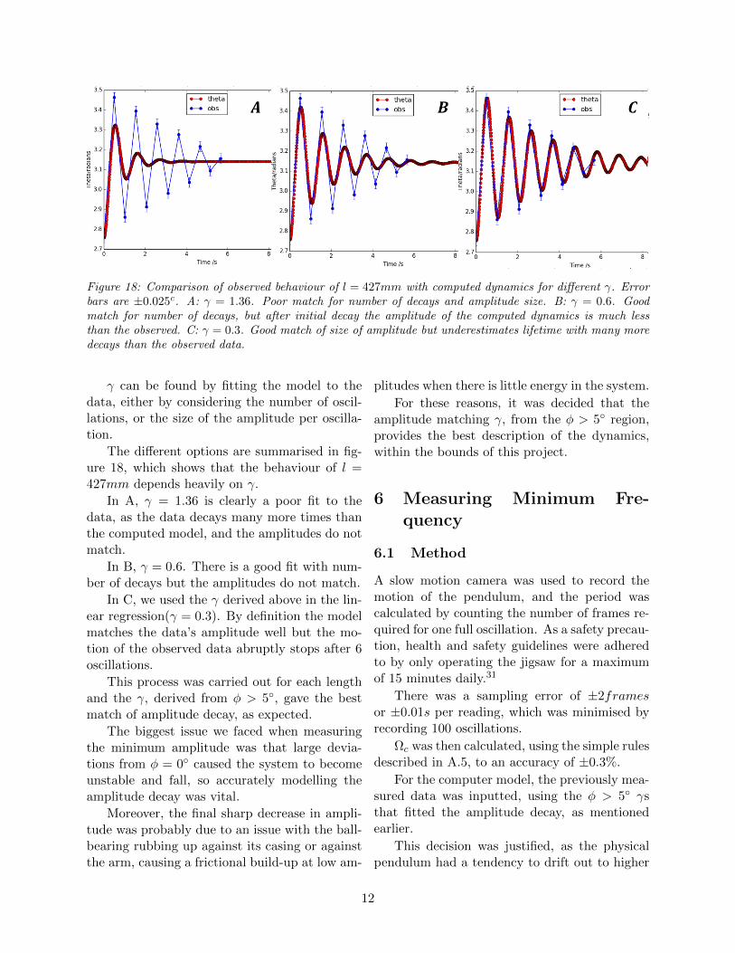
Figure 18: Comparison of observed behaviour of l = 427mm with computed dynamics for di↵erent �. Errorbars are ±0.025c. A: � = 1.36. Poor match for number of decays and amplitude size. B: � = 0.6. Goodmatch for number of decays, but after initial decay the amplitude of the computed dynamics is much lessthan the observed. C: � = 0.3. Good match of size of amplitude but underestimates lifetime with many moredecays than the observed data.

� can be found by fitting the model to thedata, either by considering the number of oscil-lations, or the size of the amplitude per oscilla-tion.

The di↵erent options are summarised in fig-ure 18, which shows that the behaviour of l =427mm depends heavily on �.

In A, � = 1.36 is clearly a poor fit to thedata, as the data decays many more times thanthe computed model, and the amplitudes do notmatch.

In B, � = 0.6. There is a good fit with num-ber of decays but the amplitudes do not match.

In C, we used the � derived above in the lin-ear regression(� = 0.3). By definition the modelmatches the data’s amplitude well but the mo-tion of the observed data abruptly stops after 6oscillations.

This process was carried out for each lengthand the �, derived from � > 5�, gave the bestmatch of amplitude decay, as expected.

The biggest issue we faced when measuringthe minimum amplitude was that large devia-tions from � = 0� caused the system to becomeunstable and fall, so accurately modelling theamplitude decay was vital.

Moreover, the final sharp decrease in ampli-tude was probably due to an issue with the ball-bearing rubbing up against its casing or againstthe arm, causing a frictional build-up at low am-

plitudes when there is little energy in the system.

For these reasons, it was decided that theamplitude matching �, from the � > 5� region,provides the best description of the dynamics,within the bounds of this project.

6 Measuring Minimum Fre-

quency

6.1 Method

A slow motion camera was used to record themotion of the pendulum, and the period wascalculated by counting the number of frames re-quired for one full oscillation. As a safety precau-tion, health and safety guidelines were adheredto by only operating the jigsaw for a maximumof 15 minutes daily.31

There was a sampling error of ±2framesor ±0.01s per reading, which was minimised byrecording 100 oscillations.

⌦c was then calculated, using the simple rulesdescribed in A.5, to an accuracy of ±0.3%.

For the computer model, the previously mea-sured data was inputted, using the � > 5� �sthat fitted the amplitude decay, as mentionedearlier.

This decision was justified, as the physicalpendulum had a tendency to drift out to higher

12

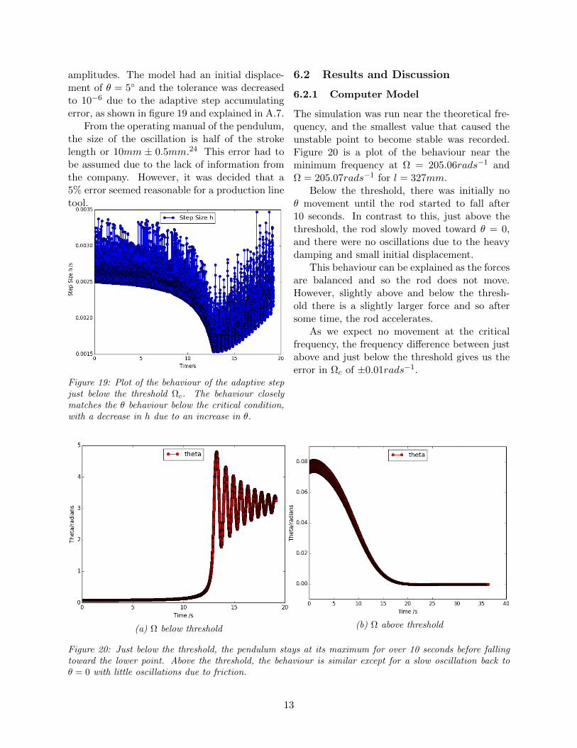
amplitudes. The model had an initial displace-ment of ✓ = 5� and the tolerance was decreasedto 10�6 due to the adaptive step accumulatingerror, as shown in figure 19 and explained in A.7.

From the operating manual of the pendulum,the size of the oscillation is half of the strokelength or 10mm ± 0.5mm.24 This error had tobe assumed due to the lack of information fromthe company. However, it was decided that a5% error seemed reasonable for a production linetool.

Figure 19: Plot of the behaviour of the adaptive stepjust below the threshold ⌦c. The behaviour closelymatches the ✓ behaviour below the critical condition,with a decrease in h due to an increase in ✓.

6.2 Results and Discussion

6.2.1 Computer Model

The simulation was run near the theoretical fre-quency, and the smallest value that caused theunstable point to become stable was recorded.Figure 20 is a plot of the behaviour near theminimum frequency at ⌦ = 205.06rads�1 and⌦ = 205.07rads�1 for l = 327mm.

Below the threshold, there was initially no✓ movement until the rod started to fall after10 seconds. In contrast to this, just above thethreshold, the rod slowly moved toward ✓ = 0,and there were no oscillations due to the heavydamping and small initial displacement.

This behaviour can be explained as the forcesare balanced and so the rod does not move.However, slightly above and below the thresh-old there is a slightly larger force and so aftersome time, the rod accelerates.

As we expect no movement at the criticalfrequency, the frequency di↵erence between justabove and just below the threshold gives us theerror in ⌦c of ±0.01rads�1.

(a) ⌦ below threshold (b) ⌦ above threshold

Figure 20: Just below the threshold, the pendulum stays at its maximum for over 10 seconds before fallingtoward the lower point. Above the threshold, the behaviour is similar except for a slow oscillation back to✓ = 0 with little oscillations due to friction.

13

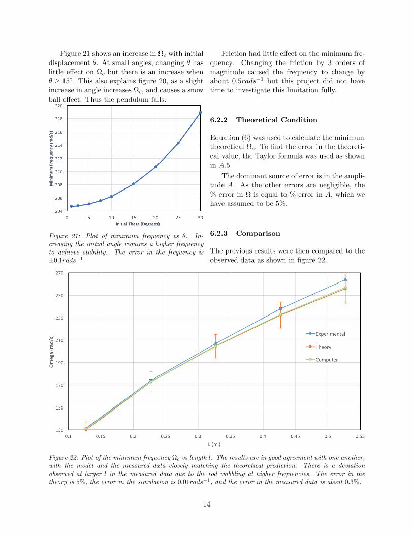
Figure 21 shows an increase in ⌦c with initialdisplacement ✓. At small angles, changing ✓ haslittle e↵ect on ⌦c but there is an increase when✓ � 15�. This also explains figure 20, as a slightincrease in angle increases ⌦c, and causes a snowball e↵ect. Thus the pendulum falls.

Figure 21: Plot of minimum frequency vs ✓. In-creasing the initial angle requires a higher frequencyto achieve stability. The error in the frequency is±0.1rads�1.

Friction had little e↵ect on the minimum fre-quency. Changing the friction by 3 orders ofmagnitude caused the frequency to change byabout 0.5rads�1 but this project did not havetime to investigate this limitation fully.

6.2.2 Theoretical Condition

Equation (6) was used to calculate the minimumtheoretical ⌦c. To find the error in the theoreti-cal value, the Taylor formula was used as shownin A.5.

The dominant source of error is in the ampli-tude A. As the other errors are negligible, the% error in ⌦ is equal to % error in A, which wehave assumed to be 5%.

6.2.3 Comparison

The previous results were then compared to theobserved data as shown in figure 22.

Figure 22: Plot of the minimum frequency ⌦c vs length l. The results are in good agreement with one another,with the model and the measured data closely matching the theoretical prediction. There is a deviationobserved at larger l in the measured data due to the rod wobbling at higher frequencies. The error in thetheory is 5%, the error in the simulation is 0.01rads�1, and the error in the measured data is about 0.3%.

14

It is clear from the data that our invertedpendulum demonstration is accurate, as the dataagrees with the theoretical model within the er-ror bars. However, there is a systematic devia-tion at longer lengths due to greater vibrations athigher frequencies. The longer rods wobbled andregularly fell out of stability as ✓ increased, sohigher frequencies were needed to reach the sta-bility condition. The computer model is slightlyhigher than the theory, which is due to thefact that the theory assumes a tiny deflection,whereas in the model we displaced the rod by✓ ⇡ 5�, and the small angular increase gives asmall increase in ⌦c as shown earlier.

The error in the theoretical results is large,and is due to the assumed error in the strokelength. However, this project did not have thetime to further investigate a method to measurethe stroke length accurately.

7 Conclusion

This project set out 3 main objectives: to builda robust working demonstration of an invertedpendulum, to write an algorithm that can beused to test the limits of dynamic stability, andto experimentally measure the friction and theminimum frequency condition.

The results in section 6 have shown thatthe demonstration is accurate, with the observeddata matching the model within error. The ap-paratus proved to be robust, and will make foran inspiring and thought-provoking demonstra-tion for those familiar with the simple pendu-lum. However, more work could be done in elim-inating the friction and mechanical noise in theapparatus, by acquiring a more expensive bear-ing. Also, as the deflection is proportional tol3, a small decrease in the pendulum arm shouldgreatly decrease the deflection. The dominantsource of error was due to the error in the strokelength, and with time this could be easily mea-sured to increase the accuracy. The friction wasmeasured and shown to fit the data. However asfeatures from n = 0 and n = 2 were observedin the data, one could record the motion using aparticle tracking system and calculate the exact

value of n.The computer model was shown to be an ac-

curate simulation with a working adaptive step.The model was a useful tool as it allowed us tofocus on the physical system in the absence ofmechanical vibrations. The simulation also al-lowed an investigation into the limitations of thestability condition, and it was shown that thesize of the deflection increased ⌦c, which is nottaken into account in the theory.

The simulation could be used in more detailto investigate the e↵ects of friction on the sys-tem. Although it was shown that friction causedlittle e↵ect to the condition over a small range of�s, the program could be run over many ordersof magnitude of � to prove this rigorously.

Alternatively, the model could be used to es-tablish whether resonances can be manipulatedto make the system jump from the lower to theupper stable point, and these results can be com-pared experimentally with the jigsaw.

As the equation of motion is analogous tothe Mathieu equation, this project’s results canbe related to a wide range of physical systemswith just a change of variables. Thus the obser-vation that higher displacements from the verti-cal require larger stabilising frequencies has in-teresting implications in a number of fields, andpotentially deserves further investigation.

References

1 P. Machamer and B. Hepburn. Galileo andthe pendulum: Latching on to time. In ThePendulum: Scientific, Historical, Philosoph-ical and Educational Perspectives, pages 99–113. 2005.

2A. Stephenson. On induced stability. Philo-sophical Magazine Series 6, 15(86):233–236,1908.

3 P. L. Kapitza. Dynamic stability of the pendu-lum when the point of suspension is oscillating.J. Exp. Theor. Phys., 21(5):588–597, 1951.

4 P. L. Kapitza. Pendulum with vibrating axisof suspension. Usp. Fizi. Nauk, 44(1):7–20,1954.

15

5M M Michaelis. Stroboscopic study of the in-verted pendulum. Am. J. Phys., 53(11):1079–1083, 1985.

6M M Michaelis and T Woodward. An invertedliquid demonstration. American Journal ofPhysics, 59(9):816–821, 1991.

7 J A. Blackburn, H. J. T. Smith, andN Grønbech-Jensen. Stability and Hopf Bifur-cations in an Inverted Pendulum. AmericanJournal of Physics, 60(10):903–908, 1992.

8H P Kalmus. The inverted pendulum. Am. J.Phys., 874:1–28, 1970.

9A. B. Pippard. The inverted pendulum. Eur.J. Phys, 203, 1987.

10 E. Butikov. An improved criterion forKapitza’s pendulum stability. Journal ofPhysics A: Mathematical and Theoretical,44(29):295202, 2011.

11 L Ruby. Applications of the Mathieu equation.American Journal of Physics, 64(1):39, 1996.

12R Ramachandran and M Nosonovsky. Vibro-levitation and inverted pendulum: parametricresonance in vibrating droplets and soft mate-rials. Soft Matter, 10(26):4633, 2014.

13W Paul. Electromagnetic Traps for Chargedand Neutral Particles (Nobel Lecture). Ange-wandte Chemie International Edition in En-glish, 29(7):739–748, 1990.

14N. P. Armitage. Cuprate superconduc-tors:Dynamic stabilization? Nature materials,13(JULY):665, 2014.

15 E Butikov. On the dynamic stabilization ofan inverted pendulum. American Journal ofPhysics, 69(7):755, 2001.

16 E. Becker and G. K. Mikhailov. Theoreticaland Applied Mechanics. Springer Science &Business Media, 1972.

17 F. S. Crawford. Damping of a simple pendu-lum. American Journal of Physics, 43(3):276–277, 1975.

18D. Tong. Lectures on Classical Dynamics. Uni-versity of Cambridge, 2015.

19 F. M. Phelps and J. H. Hunter. An AnalyticalSolution of the Inverted Pendulum. AmericanJournal of Physics, 33(1965):285, 1965.

20 F. J. Vesely. Computational Physics: An intro-duction. Springer Science & Business Media,2nd edition, 2012.

21 J. Kiusalaas. Numerical Methods in Engineer-ing with Python. Cambridge University Press,2nd edition, 2010.

22H. J. T. Smith and J. A. Blackburn. Exper-imental study of an inverted pendulum. Am.J. Phys, 60(12):909–911, 1992.

23Harvard University. Harvard Natural ScienceDemonstrations.

24Wickes PSJ800X Jigsaw Manual. 2016.

25 S. Timoshenko. History of strength of materi-als. McGraw-Hill New York, 1953.

26 Elastic Properties and Young Modulus forsome Materials, 2012.

27R. A. Serway. Physics for Scientists and En-gineers. Saunders College Publishing, 2nd edi-tion, 1986.

28TLP library DoITPoMS. Sti↵ness of long fibrecomposites, 2015.

29 J. P. Davim. Machinability of Fibre-ReinforcedPlastics. Walter de Gruyter GmbH & Co KG,2015.

30 PlumAmazing. PixelStick 2 Version 2.9, 2017.

31Health and Safety Executive UK. Hand-armvibration at work: A brief guide. 2012.

16

A Appendix

A.1 Derivation of Lagrangian

The Lagrangian method allows us to describe thephysical system in terms of the energies, ratherthan Newtonian time varying particle forces. Wedefine the Lagrangian as:

L = T � V (19)

where V is the gravitational potential energy andT is the sum of kinetic energies.

To find the moment of inertia consider a uni-form rod with COM ↵l. The moment of inertiacan be found from its definition:

ICOM =

Zx2dm =

M

l

Z (1�↵)l

�↵lx2dx

ICOM = �Ml2 =Ml2

3(1� 3↵+ 3↵2)

�(↵) =1

3(1� 3↵+ 3↵2) (20)

The above definition can be used as we as-sume the radius of the rod is much shorter thanthe length l.

The total kinetic energy is found by consid-ering the translational movement of the COM atvelocity vCOM , and the energy of rotation aboutthe COM:

T =1

2mv2COM +

1

2ICOM ✓

2 (21)

The linear velocity v2G is found by consideringtime derivative of the co-ordinates, x and y:

v2COM = (↵l✓)2 + a2 + 2a↵l✓ sin ✓ (22)

Thus we can fully describe the pendulum usingthe Lagrangian by combining (21) and (19):

L =1

2m⇥(↵l✓)2+ a2+2a↵l✓ sin ✓

⇤+

1

2ICOM ✓

2

�mg(↵l cos ✓ + a(t))

A.2 Full derivation of Minimum Fre-

quency

By writing ✓ as ✓ = ✓1 +C cos⌦t+ S sin⌦t anddi↵erentiating we find that:

✓ = ✓1+C cos⌦t�⌦C sin⌦t+S sin⌦t+⌦S cos⌦t

✓ = ✓1 + C cos⌦t� 2⌦C sin⌦t� C⌦2 cos⌦t

+ S sin⌦t+ 2⌦S cos⌦t� S⌦2 sin⌦t

Assuming C and S are small, we can use the an-gle formulas to write:

sin ✓ ⇡ sin ✓1 + cos ✓1(C cos⌦t+ S sin⌦t)

To derive the equation of motion for ✓1 we willconsider only the constant terms and the termswith frequency ⌦. The constant terms give:

✓1 � f(↵)(g

lsin ✓1 +

a⌦2

2l2C cos ✓1) = 0

where f(↵) = ↵↵2+�

. Next consider the coe�-cients of cos⌦t and sin⌦t:

�Cl2⌦2 � f(↵)glC cos ✓1 = �f(↵)A⌦2l sin ✓1

� Sl2⌦2 � glS cos ✓1 = 0

which are solved by S = 0 and

C =f(↵)A⌦2 sin ✓1

⌦2l + f(↵)g cos ✓1

As ⌦2 � g/l, C ⇡ f(↵)A sin ✓1/l, and so canderive the equation of motion for ✓1:

✓1 + f(↵)(A2⌦2f(↵)

2l2� g

l)sin✓1 = 0

A.3 Friction

The friction is included in the equation of mo-tion by using the dissipation function. If a forceacts on a particle i in the x-direction, the powerfunction is defined such that:

Fi,x =�P

�xi(23)

17

By integrating (7), we can find the power func-tion:

P = � K

n+ 1v(n+1)

Zsign(v)n+1dv

= � K

n+ 1(↵l✓)(n+1)

Zsign(✓)n+1d✓ (24)

where we have used sign(v) = sign(✓) Thus us-ing these definitions can solve for F✓ and add itinto the Lagrangian:

F✓ =�P

�✓= �sign(✓)n+1K(↵l)n+1(✓)n

In order to get equation into the same formof the SHM equation we can relabel the coe�-cient as � as for this report we only consider the✓ dependence:

F✓ = �sign(✓)n+1�(✓)n

This means that when choosing � we will beaware of varying orders of magnitude dependingon n.

A.4 Full derivation of RKF Method

The RKF method is embedded, where two ap-proximations for the solution are made at eachstep, one of order 4 and one of order 5. Depend-ing on the agreement of the two answers, h isaccepted, increased or decreased.

This is beneficial computationally as one ex-tra calculation allows the algorithm to adapt thestep size h to a specified accuracy, thus remov-ing the issue of guessing the optimal value of h.Each step requires 6 calculations:

K0 = hF(x, y)

Ki = hF(x+Aih, y+i�1X

j=0

BijKj), i = 1, 2, ..., 5

(25)

The approximations of the next step are foundusing the values for Ki. For the fourth order

formula(y4) and fifth order formula(y5):

y5(x+ h) = y(x) +5X

i=0

CiKi (26)

y4(x+ h) = y(x) +5X

i=0

DiKi (27)

The coe�cients (Ai, Bij , Ci, and Di) are theCash-Karp coe�cients and are summarised inthe Butcher tableau.21

The solution is advanced by y5 whilst y4 isused to estimate the truncation error. This isthe error of estimating an infinite sum as a finitesum, which goes as O(hn) for a nth order RKmethod.

The magnitude of the per step error, e(h),is taken as the root-mean-square di↵erence be-tween the two formulas, E(h) = y5 � y4:

e(h) = E(h) =

vuut 1

n

n�1X

i=0

E2i (h) (28)

with this solution cheap computationally as thetwo formulas evaluate the function at the samepoints.

The truncation error arises from the root-mean-square di↵erence between the two formu-las, E(h) = y5 � y4.

This estimated local error, e, is then used toadjust the step-size so that the error is approx-imately equal to required tolerance ✏. As thetruncation error for fourth order goes as O(h5),if we perform a step h1 with error e1, we cancalculate the optimal step-size h2 that gives anerror equal to ✏:

h2 = 0.9h1⇣e(h1)

✏

⌘ 15

(29)

The extra 0.9 is added as a small margin of safetydue to the approximation earlier. If h2 � h1,then h1 is accepted, otherwise the integration isrepeated with h2.

Additionally as e(h) is a very conservative es-timate for the actual error, the overall toleranceis the same as each local tolerance. For largenumbers of steps, this becomes no longer valid

18

and so ✏local will be decreased accordingly.

A.5 Error Calculation

When calculating errors in this project, we willconsistently use the Taylor expansion method. Ifwe have some function f(x, y, z) the error in fto first order will be calculated using:

�2f =

✓�f

�x

◆2

�2x +

✓�f

�y

◆2

�2y +

✓�f

�z

◆2

�2z (30)

We can use this general formula to derivesimpler forms for specific circumstances, namelyf = x+ y and f = x

y .For f = x+ y, (30) becomes:

�2f = �2x + �2y (31)

and for f = xy :

✓�f

f

◆2

=

✓�xx

◆2

+

✓�yy

◆2

(32)

Error in � is found from:

�2� =

✓��

�X

◆2

�2� (33)

where X = ln( ✓max✓0

). The error �t is ne-glected as �t << �X

The error of X is also needed. Using the prop-erties of logs, it is easy to show that:

�x =p2� ✓0✓max

��✓0 (34)

with an extra factor ofp2 arising from the fact

�✓0 = �✓max

Error in angular frequency is found from mul-tiplying the percentage error in the period by ⌦as the relationship is the same as f(x)=1/x.

�x =p2� ✓0✓max

��✓0 (35)

Error in ⌦ found by using the taylor expansionfor variables ↵, A, and l.

�2⌦ =

✓�⌦

�↵

◆2

�2↵ +

✓�⌦

�l

◆2

�2l +

✓�⌦

�A

◆2

�2A (36)

The main source of error is in the amplitudeA so we can approximate the equation to justthe term proportional to A.

A.6 n=0

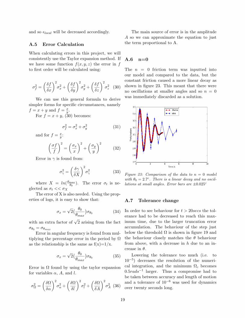
The n = 0 friction term was inputted intoour model and compared to the data, but theconstant friction caused a more linear decay asshown in figure 23. This meant that there wereno oscillations at smaller angles and so n = 0was immediately discarded as a solution.

Figure 23: Comparison of the data to n = 0 modelwith ✓0 = 2.7c. There is a linear decay and no oscil-lations at small angles. Error bars are ±0.025c

A.7 Tolerance change

In order to see behaviour for t > 20secs the tol-erance had to be decreased to reach this max-imum time, due to the larger truncation erroraccumulation. The behaviour of the step justbelow the threshold ⌦ is shown in figure 19 andthe behaviour closely matches the ✓ behaviourfrom above, with a decrease in h due to an in-crease in ✓.

Lowering the tolerance too much (i.e. to10�5) decreases the resolution of the numeri-cal integration, and the minimum ⌦c becomes0.5rads�1 larger. Thus a compromise had tobe taken between accuracy and length of motionand a tolerance of 10�6 was used for dynamicsover twenty seconds long.

19

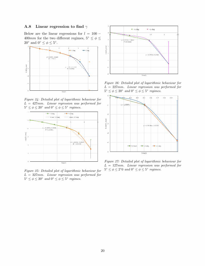
A.8 Linear regression to find �

Below are the linear regressions for l = 100 �400mm for the two di↵erent regimes, 5� � 20� and 0� � 5�.

Figure 24: Detailed plot of logarithmic behaviour forL = 427mm. Linear regression was performed for5� � 20� and 0� � 5� regimes.

Figure 25: Detailed plot of logarithmic behaviour forL = 327mm. Linear regression was performed for5� � 20� and 0� � 5� regimes.

Figure 26: Detailed plot of logarithmic behaviour forL = 227mm. Linear regression was performed for5� � 20� and 0� � 5� regimes.

Figure 27: Detailed plot of logarithmic behaviour forL = 127mm. Linear regression was performed for5� � 2�0 and 0� � 5� regimes.

20