1

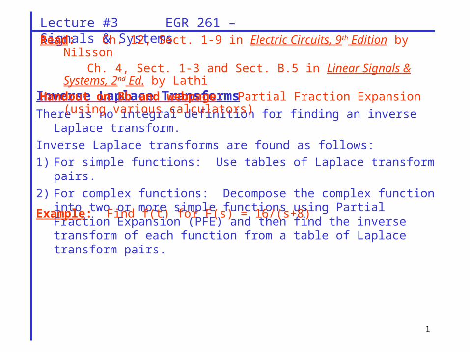
Inverse Laplace Transforms There is no integral definition for finding an inverse Laplace transform.

Inverse Laplace transforms are found as follows:

1) For simple functions: Use tables of Laplace transform pairs.

2) For complex functions: Decompose the complex function into two or more simple functions using Partial Fraction Expansion (PFE) and then find the inverse transform of each function from a table of Laplace transform pairs.

Example: Find f(t) for F(s) = 16/(s+8)

Lecture #3 EGR 261 – Signals & SystemsRead: Ch. 12, Sect. 1-9 in Electric Circuits, 9th Edition by Nilsson

Ch. 4, Sect. 1-3 and Sect. B.5 in Linear Signals & Systems, 2nd Ed. by LathiHandout on Bb and webpage: Partial Fraction Expansion (using various calculators)

2

Partial Fraction Expansion (or Partial Fraction Decomposition)Partial Fraction Expansion (PFE) is used for functions whose inverse Laplace transforms are not available in tables of Laplace transform pairs.

PFE involves decomposing a given F(s) into

F(s) = A1F1(s) + A2F2(s) + … + ANFN(s)

Where F1(s), F2(s), … , FN(s) are the Laplace transforms of known functions.

Then by applying the linearity and superposition properties:

f(t) = A1f1(t) + A2f2(t) + … + ANfN(t)

Example: Find f(t) for F(s) = 16s/(s2 + 4s + 29)

Lecture #3 EGR 261 – Signals & Systems

3

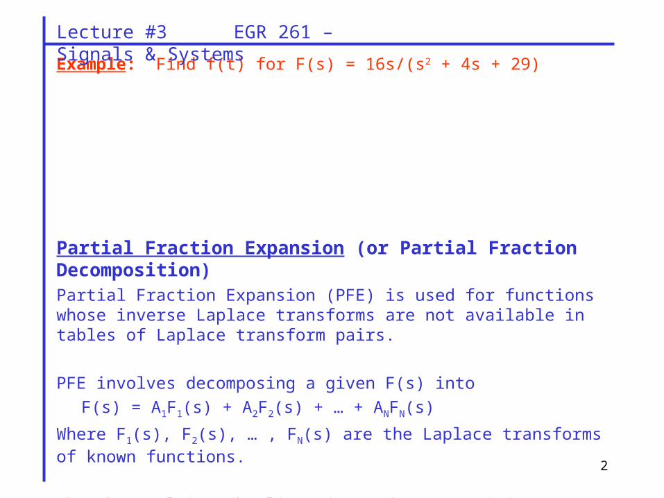
In most engineering applications,

Finding roots of the polynomials yields:

where

zi = zeros of F(s)

and

pi are the poles of F(s)

Note that:

N(s) numerator in the form of a polynomial in sF(s)

D(s) denominator in the form of a polynomial in s

1 2 M

1 2 N

K(s - z )(s - z ) (s - z )F(s)

(s - p )(s - p ) (s - p )

i

i

s = z

s = p

F(s) 0

F(s)

Lecture #3 EGR 261 – Signals & Systems

4

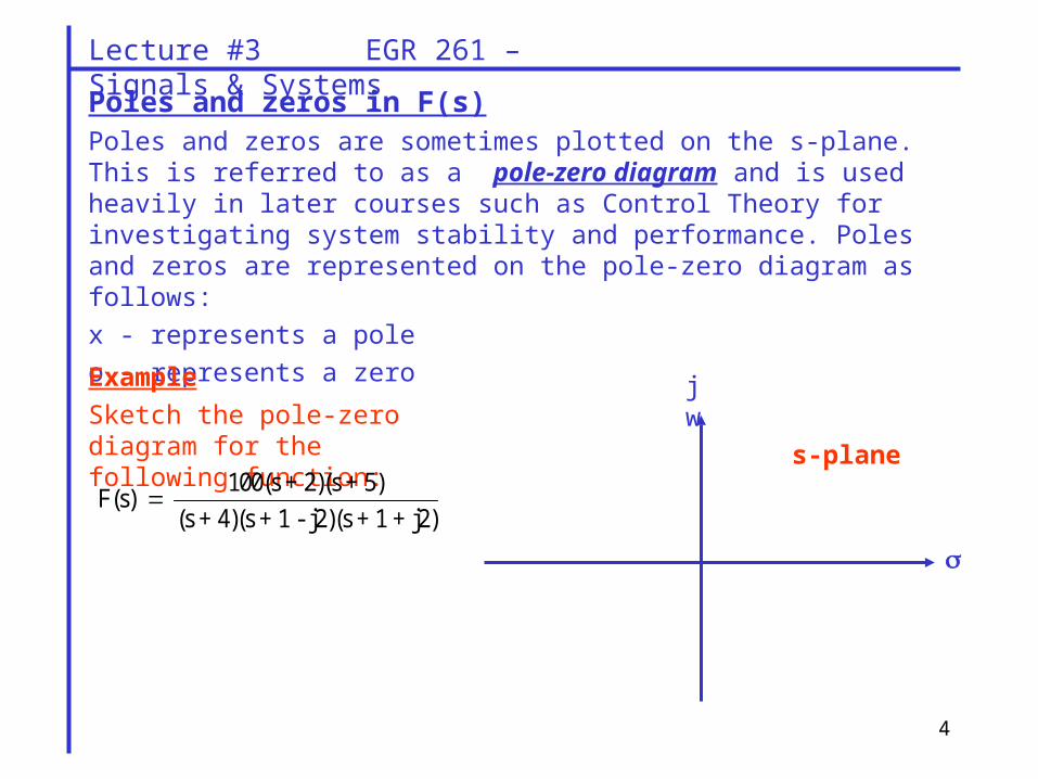
Poles and zeros in F(s)Poles and zeros are sometimes plotted on the s-plane. This is referred to as a pole-zero diagram and is used heavily in later courses such as Control Theory for investigating system stability and performance. Poles and zeros are represented on the pole-zero diagram as follows:

x - represents a pole

o - represents a zero

Example

Sketch the pole-zero diagram for the following function:

jw

s-plane100(s + 2)(s + 5)

F(s) (s + 4)(s + 1 - j2)(s + 1 + j2)

Lecture #3 EGR 261 – Signals & Systems

5

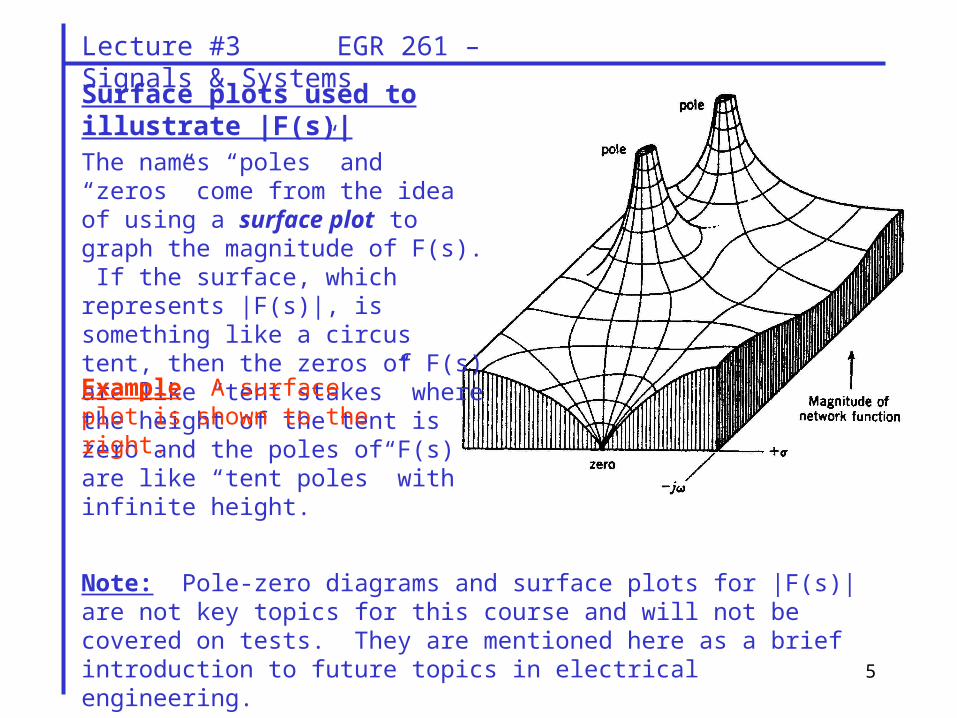
Surface plots used to illustrate |F(s)|The names “poles” and “zeros” come from the idea of using a surface plot to graph the magnitude of F(s). If the surface, which represents |F(s)|, is something like a circus tent, then the zeros of F(s) are like “tent stakes” where the height of the tent is zero and the poles of F(s) are like “tent poles” with infinite height.Example A surface plot is shown to the right.

Note: Pole-zero diagrams and surface plots for |F(s)| are not key topics for this course and will not be covered on tests. They are mentioned here as a brief introduction to future topics in electrical engineering.

Lecture #3 EGR 261 – Signals & Systems

6

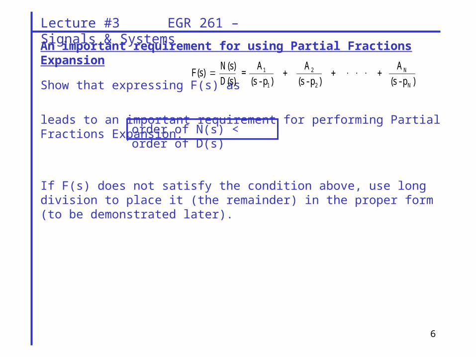
An important requirement for using Partial Fractions Expansion

Show that expressing F(s) as

leads to an important requirement for performing Partial Fractions Expansion:

If F(s) does not satisfy the condition above, use long division to place it (the remainder) in the proper form (to be demonstrated later).

order of N(s) < order of D(s)

N1 2

1 2 N

AN(s) A AF(s) =

D(s) (s - p ) (s - p ) (s - p )

Lecture #3 EGR 261 – Signals & Systems

7

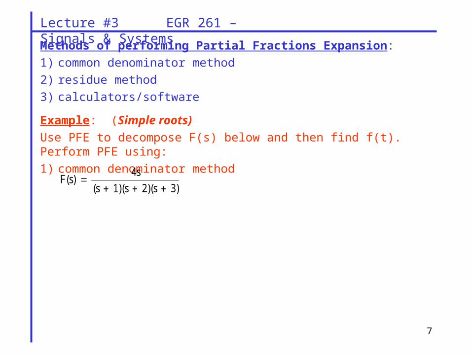
Methods of performing Partial Fractions Expansion:

1) common denominator method

2) residue method

3) calculators/software

Example: (Simple roots)

Use PFE to decompose F(s) below and then find f(t). Perform PFE using:

1) common denominator method

4sF(s)

(s 1)(s 2)(s 3)

Lecture #3 EGR 261 – Signals & Systems

8

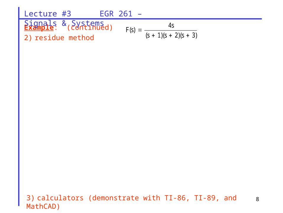
Example: (continued)

2) residue method

4sF(s)

(s 1)(s 2)(s 3)

3) calculators (demonstrate with TI-86, TI-89, and MathCAD)

Lecture #3 EGR 261 – Signals & Systems

9

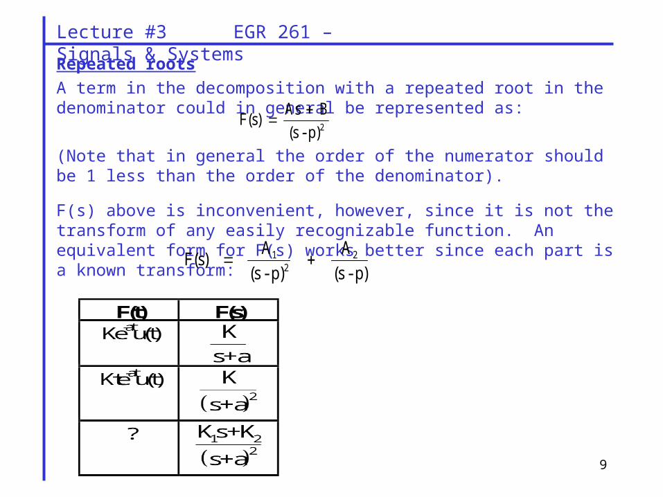
Repeated roots

A term in the decomposition with a repeated root in the denominator could in general be represented as:

(Note that in general the order of the numerator should be 1 less than the order of the denominator).

F(s) above is inconvenient, however, since it is not the transform of any easily recognizable function. An equivalent form for F(s) works better since each part is a known transform:

2

As BF(s)

(s - p)

1 22

A AF(s)

(s - p) (s - p)

Lecture #3 EGR 261 – Signals & Systems

10

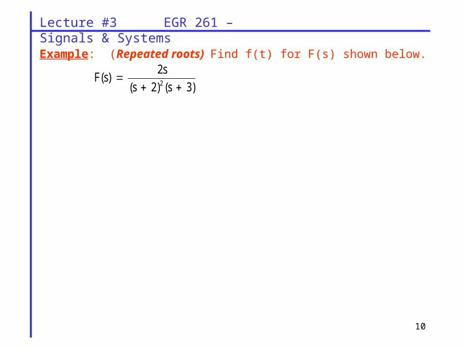
Example: (Repeated roots) Find f(t) for F(s) shown below. 2

2sF(s)

(s 2) (s 3)

Lecture #3 EGR 261 – Signals & Systems

11

Example: (Repeated roots) Find f(t) for F(s) shown below.

3

2

3 s

1 2s F(s)

Lecture #3 EGR 261 – Signals & Systems

12

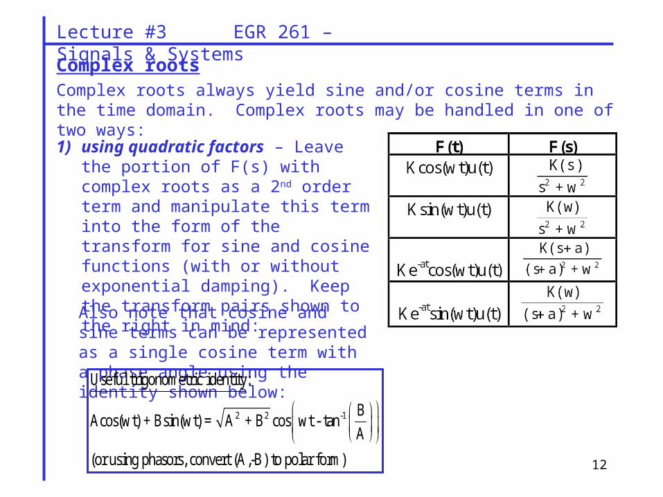
Complex rootsComplex roots always yield sine and/or cosine terms in the time domain. Complex roots may be handled in one of two ways:

Also note that cosine and sine terms can be represented as a single cosine term with a phase angle using the identity shown below:

1) using quadratic factors – Leave the portion of F(s) with complex roots as a 2nd order term and manipulate this term into the form of the transform for sine and cosine functions (with or without exponential damping). Keep the transform pairs shown to the right in mind:

2 2 -1

Useful trigonometric identity:

BAcos(wt) + Bsin(wt) = A + B cos wt - tan

A

(or using phasors, convert (A,-B) to polar form)

Lecture #3 EGR 261 – Signals & Systems

13

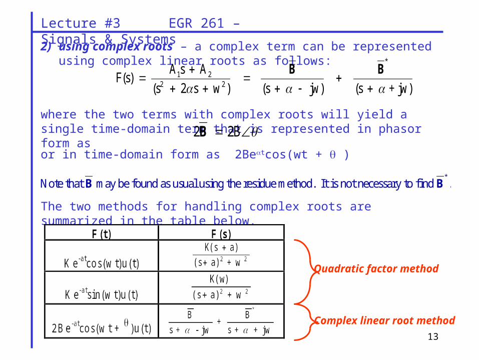
2) using complex roots – a complex term can be represented using complex linear roots as follows: *

1 22 2

A s AF(s)

(s 2 s w ) (s jw) (s + jw)

B B

where the two terms with complex roots will yield a single time-domain term that is represented in phasor form as 2 2B B

or in time-domain form as 2Betcos(wt + )

*Note that may be found as usual using the residue method. It is not necessary to fin d .B B

The two methods for handling complex roots are summarized in the table below.

Quadratic factor method

Complex linear root method

Lecture #3 EGR 261 – Signals & Systems

14

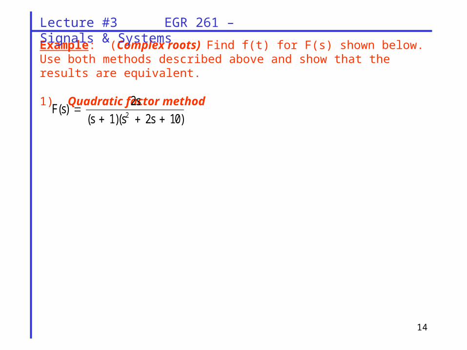
Example: (Complex roots) Find f(t) for F(s) shown below. Use both methods described above and show that the results are equivalent.

1) Quadratic factor method 2

2sF(s)

(s 1)(s 2s 10)

Lecture #3 EGR 261 – Signals & Systems

15

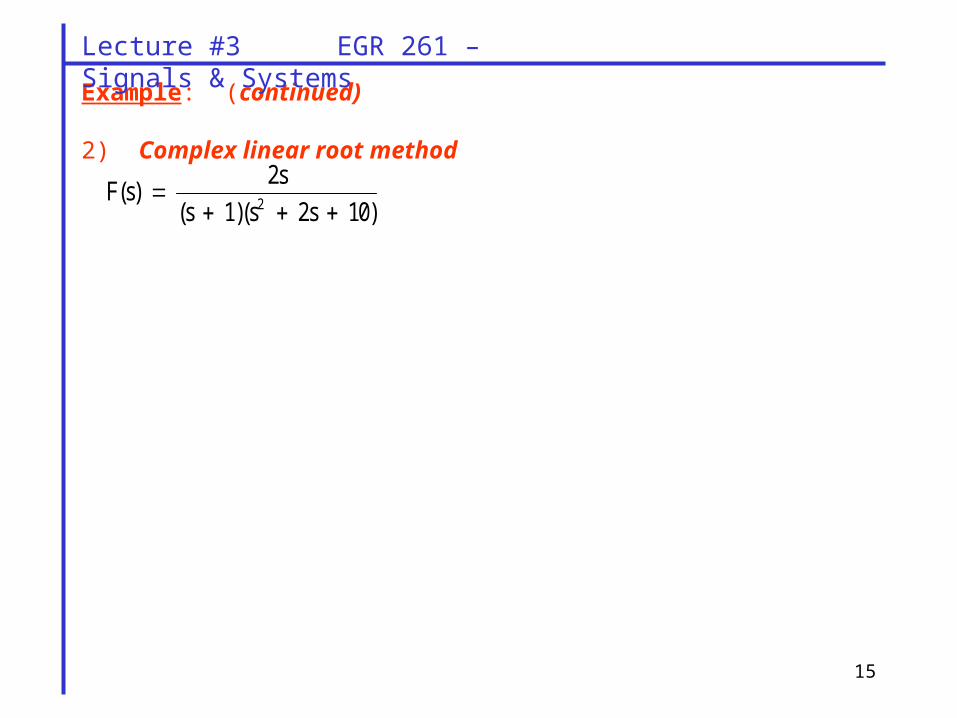
Example: (continued)

2) Complex linear root method 2

2sF(s)

(s 1)(s 2s 10)

Lecture #3 EGR 261 – Signals & Systems

16

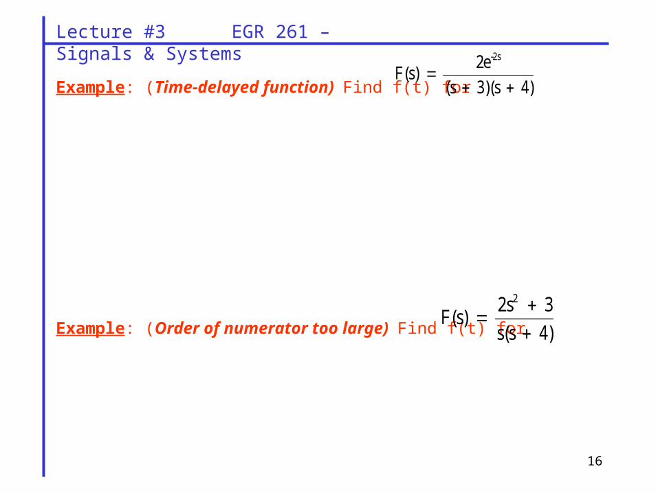
Example: (Time-delayed function) Find f(t) for -2s2e

F(s) (s 3)(s 4)

Example: (Order of numerator too large) Find f(t) for 22s 3

F(s) s(s 4)

Lecture #3 EGR 261 – Signals & Systems