Embed Size (px)
Citation preview
Inventories and the Automobile Market ∗
Adam Copeland†, Wendy Dunn‡, and George Hall§.
June 22, 2010
Abstract
This paper studies the within-model-year pricing, production, and inventory management of newautomobiles. Using new monthly data on U.S. transaction prices, we document that, for the typicalvehicle, prices fall over the model year at a 9.0 percent annual rate. Concurrently, both sales andinventories are hump shaped. To explain these time series, we formulate an industry model for newautomobiles in which inventory and pricing decisions are made simultaneously. The model predictsthat automakers’ build-to-stock inventory management policy substantially influences the time-seriesof prices and sales, accounting for four-tenths of the price decline observed over the model year.
Keywords: dynamic pricing, revenue management, discrete-choice demand estimation, build-to-stock in-ventory policyJEL classification: D21, D42, E22, L11, L62
∗We thank Ana Aizcorbe, Steve Berry, Andrew Cohen, Gautam Gowrisankaran, Amil Petrin, John Rust, John Stevens, andparticipants at numerous conferences and seminars for their helpful comments. We also received valuable comments from theeditor and three referees. Finally we thank Bob Schnorbuss for helping us obtain and interpret the data from J.D. Power andAssociates. George Hall gratefully acknowledges financial support from the Alfred P. Sloan Foundation. The views expressed inthe paper are those of the authors and not necessarily reflective of views at the Board of Governors, the Federal Reserve Bank ofNew York, or the Federal Reserve System.
†Research and Statistics, Federal Reserve Bank of New York, 33 Liberty St., New York, NY 10045; e-mail:[email protected] ; http://www.copeland.marginalq.com
‡Division of Research and Statistics, Board of Governors of the Federal Reserve System, Mail Stop 82, 20th and C Streets,NW, Washington DC 20551; e-mail: [email protected]
§Department of Economics, Brandeis University, Waltham, MA 02454; e-mail: [email protected]
1
Two common features of durable goods markets are high levels of inventories relative to sales and
declining prices over the product cycle. There has been substantial research explaining why durable goods
prices decline, with most existing theories focusing on intertemporal price discrimination (e.g. Stokey,
1979; and Conlisk, Gerstner and Sobel, 1984) or fashion (e.g. Lazear, 1986; Pashigian, 1988; and Pe-
sendorfer, 1995). We build on this body of work by emphasizing the significant role that firm-held inven-
tories can play in explaining price declines.
We focus on automakers, the quintessential durable goods producer. We begin by constructing a
monthly dataset on transaction prices, sales, and inventories for Big Three vehicles. We document four
stylized facts: (i) average retail prices, net of rebates and incentives, decline by 9 percent at an annual
rate; (ii) for about half the calendar year, automakers simultaneously sell two vintages of the same model,
during which the older vintage sells for a 9 percent discount; (iii) sales and inventories are humped-shaped
over the product cycle; and (iv) the mean ratio of inventories to sales is 75 days.
To explain these stylized facts, we develop and parameterize a two-sided industry model. We describe
the firm as a dynamic inventory control problem. The joint production/pricing decision we model is a clas-
sic issue in the operations research literature going back to Whiten (1955) and Karlin and Carr (1962).1 We
extend the theory by allowing the firm to sell two vintages simultaneously, which is a frequent occurrence
in the automobile industry (the second stylized fact). Further, since Hamermesh (1989) and Bresnahan
and Ramey (1994) document that durable good manufactures frequently adjust their rate of production by
shutting down the plant for a week or two at a time, we incorporate the non-convex cost structure from
Hall (2000) into the model to induce our fictional producer to mimic the observed production-bunching
behavior.
On the consumer’s side, we estimate preferences for automobiles by employing the econometric
methodology developed in the discrete-choice literature (for example, Berry, Levinsohn, and Pakes, 1995;
Goldberg, 1995; and Petrin, 2002; to name a few). Our approach differs from the standard one in three
ways: First, motivated by Kahn (1987, 1992) who finds that inventories are productive in generating greater
sales at a given price, we include an inventory-based measure of variety in the consumer’s indirect utility
function. This allows us to compute by how much demand changes when automobiles alter their stock of
inventories. Second, we estimate our demand-side model at a quarterly, rather than an annual, frequency
using transaction rather than list prices; thus, we can estimate how the demand curve shifts throughout1Federgruen and Heching (1999) and Elmaghraby and Keskinocak (2003) provide a nice overview of the more recent revenue
management literature within operations research.
2
the model year. Third, our data let us differentiate multiple vintages of the same model. Hence, we allow
consumers to choose among multiple vintages within and across models.
In summary, inventories play two major roles in our model. On the firm’s side, inventories allow the
manufacturer to engage in cost-minimizing production bunching. On the consumer’s side, higher levels
of inventories provide more variety, thus making it easier to match consumers with their ideal vehicle.
Hence, pricing and inventory decisions are linked both through the firm’s cost structure as well as the
demand system for automobiles.
Our two-sided model provides a consistent explanation of the four stylized facts. We replicate facts (i)
and (iii) by modeling the firm as solving an inventory control problem while facing declining demand over
the product cycle. Early in the model year, the automaker sets price sufficiently high to keep sales less
than production to accumulate a large stock of inventories. Building up inventories, or following a build-
to-stock inventory management strategy, is optimal because it strengthens demand by increasing variety.
Over the remainder of the model year, our estimate of leftward-shifting demand lowers the shadow value
of inventories (i.e. the marginal cost curve), resulting in a 9.0 percent decline in the price over the entire
product cycle and an average vintage premium of 8.5 percent (fact (ii)). Because inventories are used
to both optimally schedule production and increase variety, the model is able to match the high level of
inventories relative to sales (fact (iv)).
An innovation in this paper is to explicitly model how inventories can bolster demand by increasing
the variety of vehicles available to consumers. To quantify the importance of this role for inventories, we
simulate the model under a counterfactual build-to-order strategy. When a manufacturer builds automo-
biles according to orders, the firm is able to offer consumers full variety for every product without holding
inventories. Hence, the role for inventories in bolstering demand is shut down. Under this alternative
policy, we find that automakers’ pricing strategies are significantly different: Within model-year prices
decline by 5.3 percent, roughly six-tenths of the percent price decline observed under the firms’ current
build-to-stock policy. A main result, then, is the model’s prediction that automakers’ build-to-stock in-
ventory management policy is responsible for four-tenths of the 9.0 percent decline (annual rate) in prices
over the model year. More generally, our work suggests a significant driver behind a durable good’s price
decline may be the firm’s inventory-management strategy.2
Our work builds on the macro-inventory literature. Typically, this literature recognizes a role for2Durable goods’ price declines over the product cycle are not unique to the automobile industry, having been documented for
a number of other products, including textbooks (Chevalier and Goolsbee, 2007), microprocessors (Aizcorbe and Kortum, 2005),and consumer electronics (Gowrisankaran and Rysman, 2007; and Copeland and Shapiro, 2009).
3
inventories in spurring demand, but then assumes an exogenously specified target inventory-sales ratio
into the firm’s problem.3 In contrast, our work puts more structure on the effect of inventories on demand
and provides an estimate of the elasticity between unit sales and inventories in stock. Significantly, the
optimal inventory-to-sales ratio is endogenous in our model.
In addition, our work builds on the micro-inventory literature. Work by Reagan (1982), Aguirregabiria
(1999), Zettelmeyer, and Scott Morton and Silva-Risso (2003), for example, study the interactions between
pricing and inventory management. Our work is closest in spirit to Aguirregabiria (1999) who estimates a
structural model of a retailer which accounts for the joint dynamics of prices, sales, and firm-held inven-
tories. His work demonstrates that the possibility of stockouts along with fixed ordering costs can explain
the high-low pricing schemes retailers often employ. In contrast, we focus on a durable goods market
and consider inventory’s role in increasing the variety available to consumers. We demonstrate how this
demand for inventories partly explains the observed price decline of vehicles over the product cycle.
1 Data Sources and Empirical Observations
In this section we outline our data sources and document four stylized facts.
1.1 Data Sources
To construct a dataset of transaction prices, sales, production, and inventories by model and model year in
the U.S. we combined data from two sources. The first data source includes detailed information on U.S.
retail transactions collected from a sample of vehicle dealerships. It reports prices, by model and model
year, and the distribution of model-level sales across model years. The second data source reports total
sales in North America, by country and model, and on production, by model and model year.
The first dataset was constructed by Corrado, Dunn, and Otoo (2004), using data from J.D. Power
and Associates (JDPA). JDPA collects daily transaction-level information from dealerships across the U.S.
JDPA aggregated these data to generate a monthly time-series of average price, sales, average cash rebate,
and average financial package by model and model-year (e.g. 2000 Ford Escort). Our sample covers the
period from January 1999 to January 2004 and represents 70 percent of the geographical markets in the
U.S. and roughly 15 to 20 percent of national retail transactions. JDPA attempts to precisely measure
the transaction price of a vehicle. The price they obtain includes the price of accessories (such as roof3See for example Blanchard (1983). Bils and Kahn (2000) provide a good synopsis of the different ways the inventory
literature has built in a demand for inventories outside of its production-smoothing role.
4
racks) and transportation costs but excludes aftermarket options, taxes, title fees, and other document
preparation costs. Further, JDPA adjusts this price to account for instances when a dealership undervalues
or overvalues a customer’s trade-in vehicle as part of a new vehicle sale.4 JDPA’s transaction price does
not account for incentives the customer received to help finance the purchase of the car; hence, we define
the average market price of a vehicle as the transaction price minus the cash rebate minus a measure of the
financial incentive offered by the manufacturer.5
We linked the JDPA dataset to a dataset from Ward’s Communications on the U.S. sales and North
American production of General Motors, Ford, and Chrysler (a.k.a. the Big Three). We excluded foreign
manufacturers because measuring overseas production is difficult. The sales data for the Big Three are
available only at the model level, not by model year. Therefore, we constructed estimates of sales by
model and model year using the distributions of sales across model-years in the JDPA sample. Using model
changeover dates at assembly plants, we decomposed the production data by model into observations by
model year. Finally, using the sales and production estimates by model and model year, we constructed
estimates of inventories over the sample period. All told, the work described here results in a dataset with
monthly observations, by model year, on the real average price, quantity sold, quantity produced, and
inventory held for almost all light vehicle models sold by the Big Three in the U.S. from 1999 to 2003.
1.2 Empirical Observations
As described in the introduction, we observe several stylized facts that hold across models and model years.
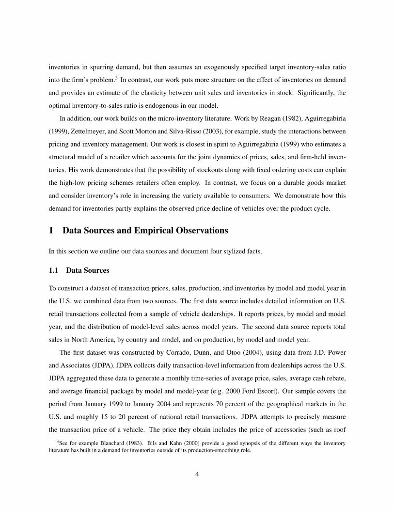
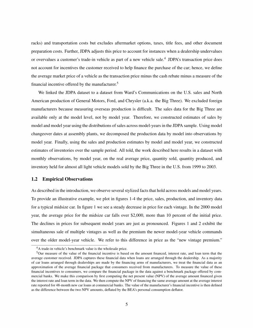
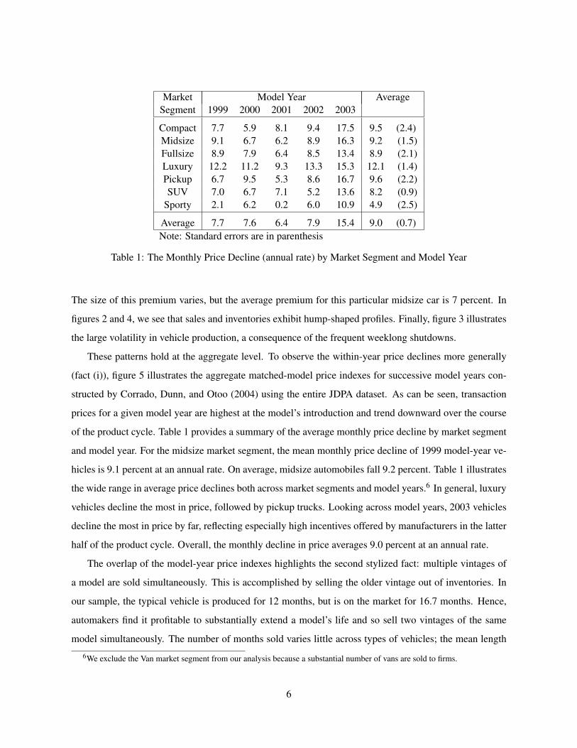
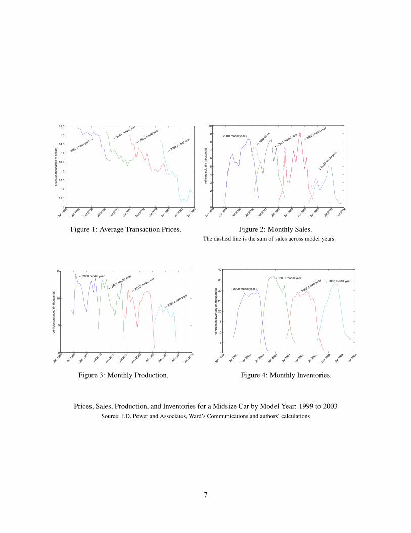
To provide an illustrative example, we plot in figures 1-4 the price, sales, production, and inventory data
for a typical midsize car. In figure 1 we see a steady decrease in price for each vintage. In the 2000 model
year, the average price for the midsize car falls over $2,000, more than 10 percent of the initial price.
The declines in prices for subsequent model years are just as pronounced. Figures 1 and 2 exhibit the
simultaneous sale of multiple vintages as well as the premium the newer model-year vehicle commands
over the older model-year vehicle. We refer to this difference in price as the “new vintage premium.”4A trade-in vehicle’s benchmark value is the wholesale price.5Our measure of the value of the financial incentive is based on the amount financed, interest rate, and loan term that the
average customer received. JDPA captures these financial data when loans are arranged through the dealership. As a majorityof car loans arranged through dealerships are made by the financing arms of manufacturers, we treat the financial data as anapproximation of the average financial package that consumers received from manufacturers. To measure the value of thesefinancial incentives to consumers, we compare the financial package in the data against a benchmark package offered by com-mercial banks. We make this comparison by first computing the net present value (NPV) of the average amount financed giventhe interest rate and loan term in the data. We then compute the NPV of financing the same average amount at the average interestrate reported for 48-month new car loans at commercial banks. The value of the manufacturer’s financial incentive is then definedas the difference between the two NPV amounts, deflated by the BEA’s personal consumption deflator.
5
Market Model Year AverageSegment 1999 2000 2001 2002 2003
Compact 7.7 5.9 8.1 9.4 17.5 9.5 (2.4)Midsize 9.1 6.7 6.2 8.9 16.3 9.2 (1.5)Fullsize 8.9 7.9 6.4 8.5 13.4 8.9 (2.1)Luxury 12.2 11.2 9.3 13.3 15.3 12.1 (1.4)Pickup 6.7 9.5 5.3 8.6 16.7 9.6 (2.2)SUV 7.0 6.7 7.1 5.2 13.6 8.2 (0.9)
Sporty 2.1 6.2 0.2 6.0 10.9 4.9 (2.5)
Average 7.7 7.6 6.4 7.9 15.4 9.0 (0.7)Note: Standard errors are in parenthesis
Table 1: The Monthly Price Decline (annual rate) by Market Segment and Model Year
The size of this premium varies, but the average premium for this particular midsize car is 7 percent. In
figures 2 and 4, we see that sales and inventories exhibit hump-shaped profiles. Finally, figure 3 illustrates
the large volatility in vehicle production, a consequence of the frequent weeklong shutdowns.
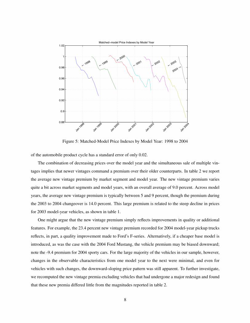
These patterns hold at the aggregate level. To observe the within-year price declines more generally
(fact (i)), figure 5 illustrates the aggregate matched-model price indexes for successive model years con-
structed by Corrado, Dunn, and Otoo (2004) using the entire JDPA dataset. As can be seen, transaction
prices for a given model year are highest at the model’s introduction and trend downward over the course
of the product cycle. Table 1 provides a summary of the average monthly price decline by market segment
and model year. For the midsize market segment, the mean monthly price decline of 1999 model-year ve-
hicles is 9.1 percent at an annual rate. On average, midsize automobiles fall 9.2 percent. Table 1 illustrates
the wide range in average price declines both across market segments and model years.6 In general, luxury
vehicles decline the most in price, followed by pickup trucks. Looking across model years, 2003 vehicles
decline the most in price by far, reflecting especially high incentives offered by manufacturers in the latter
half of the product cycle. Overall, the monthly decline in price averages 9.0 percent at an annual rate.
The overlap of the model-year price indexes highlights the second stylized fact: multiple vintages of
a model are sold simultaneously. This is accomplished by selling the older vintage out of inventories. In
our sample, the typical vehicle is produced for 12 months, but is on the market for 16.7 months. Hence,
automakers find it profitable to substantially extend a model’s life and so sell two vintages of the same
model simultaneously. The number of months sold varies little across types of vehicles; the mean length6We exclude the Van market segment from our analysis because a substantial number of vans are sold to firms.
6
11
11.5
12
12.5
13
13.5
14
14.5
15
15.5
Jan 1
999
Jul 1
999
Jan 2
000
Jul 2
000
Jan 2
001
Jul 2
001
Jan 2
002
Jul 2
002
Jan 2
003
Jul 2
003
Jan 2
004
2000 model year →← 2001 model year
← 2002 model year
← 2003 model year
pric
es (i
n th
ousa
nds
of d
olla
rs)
Figure 1: Average Transaction Prices.
0
1
2
3
4
5
6
7
8
9
10
Jan 1
999
Jul 1
999
Jan 2
000
Jul 2
000
Jan 2
001
Jul 2
001
Jan 2
002
Jul 2
002
Jan 2
003
Jul 2
003
Jan 2
004
2000 model year ↓
← 2001 model year
← 2002 model year
↓ 200
3 mod
el ye
ar
← to
tal sa
les
vehi
cles
sold
(in
thou
sand
s)
Figure 2: Monthly Sales.The dashed line is the sum of sales across model years.
0
5
10
15
Jan 1
999
Jul 1
999
Jan 2
000
Jul 2
000
Jan 2
001
Jul 2
001
Jan 2
002
Jul 2
002
Jan 2
003
Jul 2
003
Jan 2
004
← 2000 model year
← 2001 model year
← 2002 model year
← 2003 model year
vehi
cles
prod
uced
(in
thou
sand
s)
Figure 3: Monthly Production.
0
5
10
15
20
25
30
35
40
Jan 1
999
Jul 1
999
Jan 2
000
Jul 2
000
Jan 2
001
Jul 2
001
Jan 2
002
Jul 2
002
Jan 2
003
Jul 2
003
Jan 2
004
2000 model year ↓
← 2001 model year
← 2002 model year ↓ 2003 model year
vehi
cles
in in
vent
ory
(in th
ousa
nds)
Figure 4: Monthly Inventories.
Prices, Sales, Production, and Inventories for a Midsize Car by Model Year: 1999 to 2003Source: J.D. Power and Associates, Ward’s Communications and authors’ calculations
7
0.88
0.9
0.92
0.94
0.96
0.98
1
1.02Matched−model Price Indexes by Model Year
Jan 1
998
Jan 1
999
Jan 2
000
Jan 2
001
Jan 2
002
Jan 2
003
Jan 2
004
← 1998← 1999 ← 2000
← 2001← 2002
← 2003
2004 →
Figure 5: Matched-Model Price Indexes by Model Year: 1998 to 2004
of the automobile product cycle has a standard error of only 0.02.
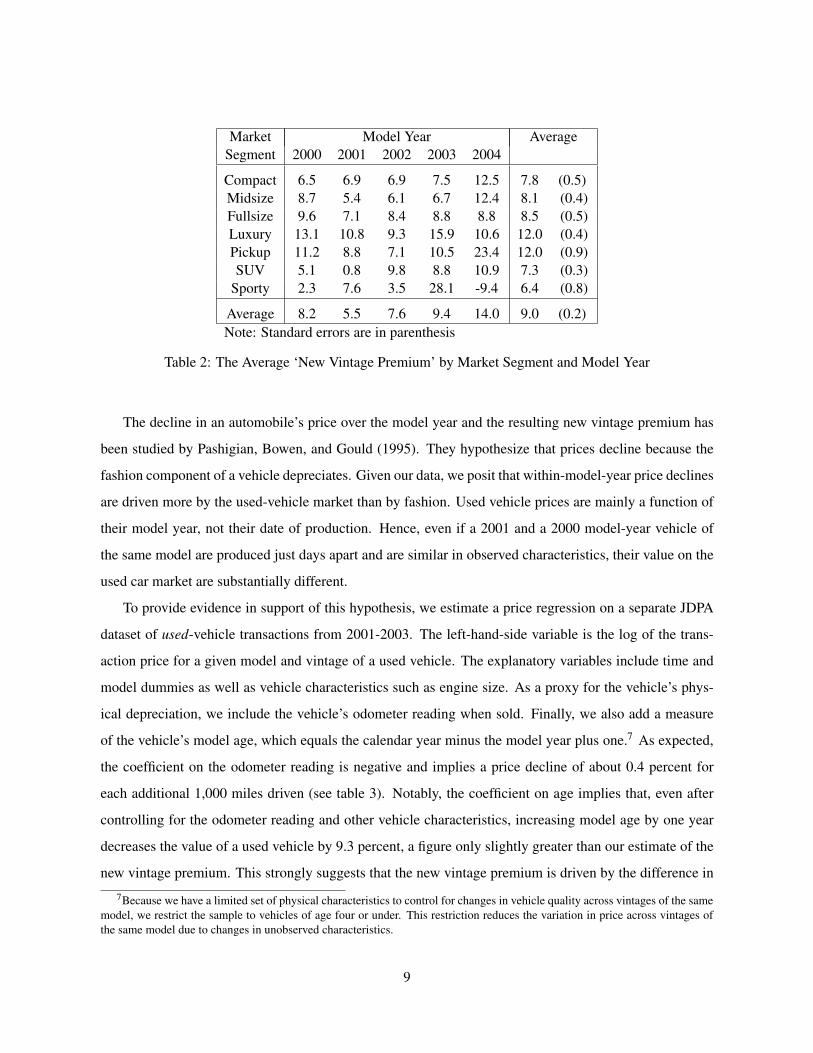
The combination of decreasing prices over the model year and the simultaneous sale of multiple vin-
tages implies that newer vintages command a premium over their older counterparts. In table 2 we report
the average new vintage premium by market segment and model year. The new vintage premium varies
quite a bit across market segments and model years, with an overall average of 9.0 percent. Across model
years, the average new vintage premium is typically between 5 and 9 percent, though the premium during
the 2003 to 2004 changeover is 14.0 percent. This large premium is related to the steep decline in prices
for 2003 model-year vehicles, as shown in table 1.
One might argue that the new vintage premium simply reflects improvements in quality or additional
features. For example, the 23.4 percent new vintage premium recorded for 2004 model-year pickup trucks
reflects, in part, a quality improvement made to Ford’s F-series. Alternatively, if a cheaper base model is
introduced, as was the case with the 2004 Ford Mustang, the vehicle premium may be biased downward;
note the -9.4 premium for 2004 sporty cars. For the large majority of the vehicles in our sample, however,
changes in the observable characteristics from one model year to the next were minimal, and even for
vehicles with such changes, the downward-sloping price pattern was still apparent. To further investigate,
we recomputed the new vintage premia excluding vehicles that had undergone a major redesign and found
that these new premia differed little from the magnitudes reported in table 2.
8
Market Model Year AverageSegment 2000 2001 2002 2003 2004
Compact 6.5 6.9 6.9 7.5 12.5 7.8 (0.5)Midsize 8.7 5.4 6.1 6.7 12.4 8.1 (0.4)Fullsize 9.6 7.1 8.4 8.8 8.8 8.5 (0.5)Luxury 13.1 10.8 9.3 15.9 10.6 12.0 (0.4)Pickup 11.2 8.8 7.1 10.5 23.4 12.0 (0.9)SUV 5.1 0.8 9.8 8.8 10.9 7.3 (0.3)
Sporty 2.3 7.6 3.5 28.1 -9.4 6.4 (0.8)
Average 8.2 5.5 7.6 9.4 14.0 9.0 (0.2)Note: Standard errors are in parenthesis
Table 2: The Average ‘New Vintage Premium’ by Market Segment and Model Year
The decline in an automobile’s price over the model year and the resulting new vintage premium has
been studied by Pashigian, Bowen, and Gould (1995). They hypothesize that prices decline because the
fashion component of a vehicle depreciates. Given our data, we posit that within-model-year price declines
are driven more by the used-vehicle market than by fashion. Used vehicle prices are mainly a function of
their model year, not their date of production. Hence, even if a 2001 and a 2000 model-year vehicle of
the same model are produced just days apart and are similar in observed characteristics, their value on the
used car market are substantially different.
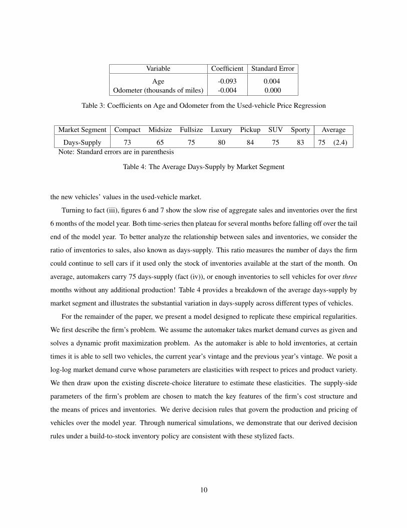
To provide evidence in support of this hypothesis, we estimate a price regression on a separate JDPA
dataset of used-vehicle transactions from 2001-2003. The left-hand-side variable is the log of the trans-
action price for a given model and vintage of a used vehicle. The explanatory variables include time and
model dummies as well as vehicle characteristics such as engine size. As a proxy for the vehicle’s phys-
ical depreciation, we include the vehicle’s odometer reading when sold. Finally, we also add a measure
of the vehicle’s model age, which equals the calendar year minus the model year plus one.7 As expected,
the coefficient on the odometer reading is negative and implies a price decline of about 0.4 percent for
each additional 1,000 miles driven (see table 3). Notably, the coefficient on age implies that, even after
controlling for the odometer reading and other vehicle characteristics, increasing model age by one year
decreases the value of a used vehicle by 9.3 percent, a figure only slightly greater than our estimate of the
new vintage premium. This strongly suggests that the new vintage premium is driven by the difference in7Because we have a limited set of physical characteristics to control for changes in vehicle quality across vintages of the same
model, we restrict the sample to vehicles of age four or under. This restriction reduces the variation in price across vintages ofthe same model due to changes in unobserved characteristics.
9
Variable Coefficient Standard Error
Age -0.093 0.004Odometer (thousands of miles) -0.004 0.000
Table 3: Coefficients on Age and Odometer from the Used-vehicle Price Regression
Market Segment Compact Midsize Fullsize Luxury Pickup SUV Sporty Average
Days-Supply 73 65 75 80 84 75 83 75 (2.4)Note: Standard errors are in parenthesis
Table 4: The Average Days-Supply by Market Segment
the new vehicles’ values in the used-vehicle market.
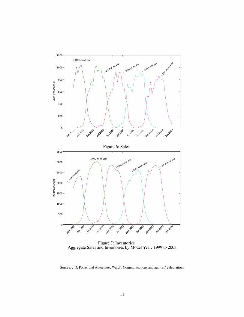
Turning to fact (iii), figures 6 and 7 show the slow rise of aggregate sales and inventories over the first
6 months of the model year. Both time-series then plateau for several months before falling off over the tail
end of the model year. To better analyze the relationship between sales and inventories, we consider the
ratio of inventories to sales, also known as days-supply. This ratio measures the number of days the firm
could continue to sell cars if it used only the stock of inventories available at the start of the month. On
average, automakers carry 75 days-supply (fact (iv)), or enough inventories to sell vehicles for over three
months without any additional production! Table 4 provides a breakdown of the average days-supply by
market segment and illustrates the substantial variation in days-supply across different types of vehicles.
For the remainder of the paper, we present a model designed to replicate these empirical regularities.
We first describe the firm’s problem. We assume the automaker takes market demand curves as given and
solves a dynamic profit maximization problem. As the automaker is able to hold inventories, at certain
times it is able to sell two vehicles, the current year’s vintage and the previous year’s vintage. We posit a
log-log market demand curve whose parameters are elasticities with respect to prices and product variety.
We then draw upon the existing discrete-choice literature to estimate these elasticities. The supply-side
parameters of the firm’s problem are chosen to match the key features of the firm’s cost structure and
the means of prices and inventories. We derive decision rules that govern the production and pricing of
vehicles over the model year. Through numerical simulations, we demonstrate that our derived decision
rules under a build-to-stock inventory policy are consistent with these stylized facts.
10
0
200
400
600
800
1000
1200Sa
les
(thou
sand
s)
Jan 1
999
Jul 1
999
Jan 2
000
Jul 2
000
Jan 2
001
Jul 2
001
Jan 2
002
Jul 2
002
Jan 2
003
Jul 2
003
Jan 2
004
↓ 1999 model year
← 2000 model year
← 2001 model year
← 2002 model year
← 20
03 m
odel
year
Figure 6: Sales
0
500
1000
1500
2000
2500
3000
3500
Inv
(thou
sand
s)
Jan 1
999
Jul 1
999
Jan 2
000
Jul 2
000
Jan 2
001
Jul 2
001
Jan 2
002
Jul 2
002
Jan 2
003
Jul 2
003
Jan 2
004
↓ 199
9 mod
el ye
ar
↓ 2000 model year
← 2001 model year
↓ 2002 model year
← 2003 model year
Figure 7: InventoriesAggregate Sales and Inventories by Model Year: 1999 to 2003
Source: J.D. Power and Associates, Ward’s Communications and authors’ calculations
11
2 An Industry Model with Overlapping Vintages
In the interest of tractability, we make several assumptions on the supply side. First, each vehicle line
within the firm can be considered a separate, independent subfirm or profit center. Hence, an automaker
is modeled as a collection of dynamic programs that can be solved independently of each other. Second,
we integrate the dealership into the automaker and consider a unified pricing decision. Third, we abstract
from bargaining by assuming that all customers who purchase during a particular period pay the same
retail price. Of course, there are many interesting questions about how the automakers decentralize their
operations both across products and between the production and marketing sides of the business.8 While
issues of vertical control and price discrimination are present in the automobile market, we are implicitly
assuming that manufactures and dealers jointly set prices to maximize their combined profits and solve the
double-marginalization problem. Furthermore, we interpret high levels of inventories nationally to reflect
high levels of inventories at all dealerships. Hence, automakers are able to coordinate with dealerships so
that there is not an uneven distribution of inventories across the country.
The automaker produces one vintage of a vehicle at a time, switching to build a newer vintage every
year. While production is exogenously limited to 52 weeks, the number of weeks a vehicle is sold is
endogenous. In particular, through the use of inventories the automaker can sell a specific vintage for
more than a year. This also implies that an automaker can choose to sell two vintages of a vehicle at the
same time. A specific vintage is labeled this year’s vintage, or the new vintage for the first 52 weeks of its
life. After 52 weeks, when it is no longer being produced, we label the specific vintage last year’s, or the
old, vintage. The automaker’s decision period is a week, where the automaker solves an infinite horizon
problem by repeatedly solving a 52-week problem. Each week the firm must decide (1) the number of
vehicles of the current model year to produce, qt ; (2) the number of days to operate the plant, Dt , the
number of shifts to run, St , and the number of hours per shift, ht ; (3) the retail price of the current vintage,
pthist ; and (4) the retail price of last year’s vintage, plast
t (if any are still in stock).
We assume that weekly sales, s jt , for each of the two vintages depend on each vintage’s own price, the
price of the other vintage, and the stock of each vintage, I jt , that is inventoried at the end of period t−1:
logs jt = µ j
t −η jt log(p j
t )+φ jit log(pi
t)+ζ jt log
�I jt
Imean
�for j, i = {this, last} and i �= j, (1)
8For example, Bresnahan and Reiss (1985) model and estimate the division of markups between automobile manufacturersand dealers. Busse, Silva-Risso and Zettlemeyer (2006) estimate how the value of manufacturer’s incentives programs are splitbetween dealers and final customers. For discussions of bargaining and price discrimination in the retail auto market see Ayresand Siegelman (1995), Goldberg (1996), Scott Morton, Zettelmeyer, and Silva-Risso (2003), and Langer (2009).
12
where µ jt is a constant term, η j
t is the own-price elasticity, φ jit is the cross-price elasticity and ζ j
t is the
own-variety elasticity. These elasticities may vary across the 52 weeks of the year. With the variety term,I jt
Imean , we seek to capture the idea that consumers are more likely to purchase a vehicle if they can find one
that matches their particular tastes. Within the automobile industry, variety means having vehicles on a
dealership lot with all possible combinations of options (e.g. color, leather interior, automatic transmis-
sion). Hence, our definition of variety translates into a measure of the number of vehicles at a dealership.
Because we do not have data at the dealership level, our proxy for variety is inventories (i.e. the number of
cars at all dealerships) divided by the mean level of inventories for the appropriate market segment. We do
not simply use the level of inventories as our measure of variety because the number of dealerships by mar-
ket segment varies. Intuitively, vehicles that appeal to buyers across the U.S. will require larger amounts
of inventory to achieve the same level of variety, relative to less popular vehicles only sold in parts of the
country. Mercedes-Benz, for example, only had 191 dealerships in the U.S. in 2002, while Honda had
959.9 Dividing through by the mean allows us to compare the inventory accumulation of popular vehicles
such as pickups, and its resulting effect on variety, to other vehicles.10
Our inventory-based measure of variety assumes that higher levels of inventory imply higher levels
of variety. Unfortunately, we do not have any direct evidence this is true nor do we have alternative
measures of variety. Nevertheless, linking higher levels of inventory with more variety in an industry with
significant product differentiation seems reasonable and is consistent with results reported in Cachon and
Olivares (2008).
Since there is no intercept with constant-elasticity demand curves, we assume that customers never
pay more for last year’s vintage than for the current vintage:
slastt = 0 if plast
t > pthist . (2)
Unsold vehicles can be inventoried without depreciation. Current production is not available for immediate
sale, so sales can be made only from the beginning-of-period inventories:
s jt ≤ I j
t . (3)9Data taken from Ward’s 2002 Automotive Yearbook.
10A natural question is why we did not use a more disaggregate mean level of inventories. After all, even within marketsegments there is variation in vehicle popularity. Given that our model/model-year inventory measures are inferred from estimatedsales and production flows, however, we are worried about the level of noise in the data at this level. Further, we would needto impute mean inventory levels for a number of models for which we do not observe a full model year (e.g. models newlyintroduced at the end of the sample).
13
Further, sales cannot be backlogged. Inventories for the current vintage follow the standard law of motion:
Ithist+1 = Ithis
t +qt − sthist . (4)
Because no vehicles for the last model year are produced during the current year, inventories for last year’s
vintage evolve according to
Ilastt+1 = Ilast
t − slastt . (5)
At the conclusion of the current model year, any unsold vehicles of last year’s vintage are scrapped at a
zero price, and this year’s vintage becomes last year’s vintage:
Ilast1 = Ithis
52 +q52− sthis52 . (6)
We assume the vehicle is assembled at a single plant. Each period, the firm must decide how many ve-
hicles of the current vintage to produce and how to organize production to minimize costs. As documented
by Hamermesh (1989) and Bresnahan and Ramey (1994) managers at durable good manufacturing plants
typically increase or decrease production by altering the length of the workweek rather than the rate of
production (i.e. the speed of the assembly line). In particular week-long plant shutdowns are frequently
employed. In the auto industry lingo these plant closures are called inventory adjustment shutdowns. In
order to allow induce the firm in our model to engage in similar production scheduling, we assume the
firm has a linear production function but faces a set of non-convex costs.
We assume the plant can operate D days a week. It can run one or two shifts, S, each day, and both
shifts are h hours long. We assume the number of employees per shift, n, and the line speed, LS, are fixed.
So the firm’s production function is:
qt = Dt ×St ×ht ×LS. (7)
We assume the firm faces a set of non-convex costs to running the plant each week. We motivate these
non-convex costs from the union contract, though we recognize that the contract structure is endogenous
and that the non-convexities may be due to the underlying technology.
From the autoworkers’ union contracts, we know that workers on the second shift receive a 5 percent
premium above the first shift wage. Any work in excess of eight hours a day, and all Saturday work, are
paid at a rate of time and a half. Employees who work fewer than 40 hours per week must be paid 85
percent of their hourly wage times the difference between 40 and the number of hours worked. This “short
week compensation” is in addition to the wages paid for hours actually worked. If the firm chooses to not
14
operate a plant for a week, the workers are laid off. Laid-off workers receive 95 cents on the dollar of their
40 hour pay in unemployment compensation. Of these 95 cents, the firm pays about 65 cents.
Given such a labor contract, if the firm decides to produce q vehicles, it must then choose how many
days to operate the plant, how many shifts to run, and how many hours to run each shift to minimize its
cost of production. Given these choices, the firm’s week t cost function is expressed as
c(Dt ,St ,ht |qt) = γqt + (w1 + I(St = 2)w2)× (Dthtn+max[0,0.85(40−Dtht)n] (8)
+max[0,0.5Dt(ht −8)n]+max[0,0.5(Dt −5)8n])+0.65w140(2−St)n,
where n is the number of employees per shift, and w1 and w2 are the hourly wage rates paid to the first-shift
and second-shift workers, respectively. γ is the per vehicle material cost and incorporates all costs (such
as materials, energy, transaction) that do not depend on the allocation of production over the week. The
first term within the brackets represents the straight-time wages paid to the production workers, and the
subsequent terms capture the 85 percent short-week rule and the overtime premia. The last term is the
unemployment compensation bill charged to the firm. This cost function is piecewise linear with kinks
at one shift running 40 hours per week and two shifts running 40 hours per week. This implies that
the firm minimizes average cost by operating the plant with either one shift or two shifts for 40 hours
per week. When the plant operates below its minimum efficient scale, the cost-minimizing production
schedule involves bunching production by oscillating between running two 40-hour shifts for a several
weeks and then shutting down the plant for a week.11
The firm’s objective is to maximize the present value of the discounted stream of profits. For each
model year the automaker’s problem is to maximize52
∑t=1
�1
1+ r
�t−1 �plast
t slastt + pthis
t sthist − c(Dt ,St ,ht |qt)
�+
�1
1+ r
�52
V (Ilast1 ,0,1) (9)
subject to (1)-(7) and where c(D,S,h|q) is given by (8). The term V (Ilast1 ,0,1) is a continuation value,
which we now define.
Let V (Ilast , Ithis, t) be the optimal value at week t for the firm that holds in inventory Ilast of last year’s
vintage and Ithis of this year’s vintage. Then the firm’s value function for t = 1,2, ...,51 can be written:
V (Ilast , Ithis, t) = maxpthis,plast ,q
�plastslast + pthissthis − min
D,S,hc(D,S,h|q) +
11+ r
V (Ilast − slast , Ithis +q− sthis, t +1)�
(10)
11If we assumed a convex cost function, the main results of this paper would still go through. We incorporate this non-convexcost structure because one reason automobile firms hold inventories is to facilitate plant shutdowns due to scheduled holidaysor a desire to reduce production. In other work, Copeland and Hall (forthcoming) compare the response to demand shocks of aautomobile firm-level model with convex costs to one with non-convex costs. The model with non-convex costs more accuratelyreplicates matches the covariance between production, price, and sales.
15
subject to (1), (2), (3), and (7) and where c(D,S,h|q) is given by (8). At week 52, this year’s vintage
becomes last year’s vintage, and so the value function is
V (Ilast , Ithis,52) = maxpthis,plast ,q
�plastslast + pthissthis−min
D,S,hc(D,S,h|q) +
11+ r
V (Ithis +q− sthis,0,1)�
. (11)
Following a suggestion by John Rust, we merge the 52 value functions into a single time-invariant
Bellman equation:
V (Ilast ,0,1) = max{pthis
t ,plastt ,qt ,Dt ,St ,ht}
�52
∑t=1
�1
1+ r
�t−1 �plast
t slastt + pthis
t sthist − c(Dt ,St ,ht |qt)
�(12)
+�
11+ r
�52
V (Ithis52 +q52− sthis
52 ,0,1)
�.
For a given parameter vector, we carried out the following steps to solve for the fixed point: (1) Guess
an initial value for V (Ilast ,0,1); (2) solve the 52 Bellman equations in (10) and (11) through backward
recursion; (3) compute a new value for V (Ilast ,0,1) through policy iteration; and (4) repeat steps 2 and 3
until a fixed point is reached. More details on the solution method are provided in the appendix.
3 Parameterizing the Model
There are a large number of parameters in this model. For the demand-side parameters we employ a
discrete-choice methodology to estimate consumers’ preferences over automobiles. We then use these
estimates to compute the intercepts, own-price elasticities, cross-price elasticities, and own-variety elas-
ticities that are parameters in the market demand function, equation (1). For the supply-side parameters,
we choose some values based on published information on assembly plants. The remaining values are set
to match a set of first moments in the data.
3.1 Demand-side parameters
Overview: Following Berry, Levinsohn, and Pakes (1995), henceforth BLP, we construct the demand
system by aggregating over the discrete choices of heterogeneous individuals. The utility derived from
choosing an automobile depends on the interaction between a consumer’s characteristics and a product’s
characteristics. Consumers are heterogeneous in income as well as in their tastes for certain product
characteristics. We distinguish between two types of product characteristics: those that are observed by
the econometrician (such as size and horsepower), which are denoted by X ; and those that are unobserved
by the econometrician (such as styling or prestige), which are denoted by ξ. We allow for households’
16
distaste for price, denoted by α, to vary from quarter to quarter, capturing the possibility that different
types of households show up to purchase a new automobile at different times of the year. We specify the
indirect utility derived from consumer i purchasing product j in period t as
ui jt = Xjtβ+ξ jt −4
∑q=1
1dt=qαiq p jt +∑k
σkνikx jkt + εi jt , (13)
where p jt denotes the price of product j in period t and x jkt ∈ Xj is the kth observable characteristic of
product j. Let dt denote the quarter of the automotive year into which period t falls, and let 1dt=q be
an indicator variable equal to 1 when dt is equal to q ∈ {1,2,3,4}. The term Xjtβ + ξ jt , where β are
parameters to be estimated, represents the utility from product j that is common to all consumers, or a
mean level of utility, δ jt . Consumers then have a distribution of tastes for each observable characteristic.
For each characteristic k, consumer i has a taste νik, which is drawn from an independently and identically
distributed (i.i.d.) standard normal distribution. The parameter σk captures the variance in consumer tastes.
The term αiq measures a consumer’s distaste for price. Following Berry, Levinsohn, and Pakes (1999), we
assume that αiq = αqyi
, where αq is a parameter to be estimated and yi is a draw from the income distribution.
Finally, εi jt is distributed i.i.d. type 1 extreme value.
Consumers choose among the j = 1,2, . . . ,J automobiles in our sample and the outside good, which
represents the choice not to buy a new automobile from the Big Three. Consumers maximizes utility, and
market shares are obtained by aggregating over consumers.
Implementation: As described in section 1, our sample includes data on the Big Three firms over the
five-year period from February 1999 to January 2004. There are 638 observations of unique model and
model-year vehicles. Industry wisdom is that consumers sometimes time their vehicle purchase decisions,
for example to take advantage of end-of-month sales. As such, we believe our static demand model is
better suited to analyzing quarterly, rather than monthly, data. Hence, we aggregate sales and prices to the
quarterly frequency.
As was done in previous research, we link sales and prices to the characteristics of the base model
to produce a vehicle-quarter observation.12 Following Nevo (2001), we use model-level fixed effects as
the matrix of observable characteristics used to compute the mean utility of a product. We supplement
these dummies with a quadratic time trend, model year dummies, and measures of congestion, variety,
and “newness”. The congestion dummy variable draws from the work of Ackerberg and Rysman (2005),12Information on vehicle characteristics were taken from Automotive News’s Market Data Book (various years).
17
who demonstrate the importance of controlling for variation in the choice set when estimating consumers’
price elasticities. Because of the overlap in model years, households face large variation in the number
of products offered over time. To capture this effect, we use an indicator variable equal to 1 when two
vintages of the same model are sold in the same quarter. The variety term, to our knowledge, has not
previously been incorporated into the BLP framework. We use the definition of variety described above
(see section 2), the ratio of inventories to the mean level of inventories for the appropriate market segment.
To better capture the substitution patterns between two vintages of the same model, we use a “newness”
dummy variable equal to one if a model has been sold for less than a year.
Finally, measures of acceleration and dimensions, along with the newness dummy variable and con-
stant term are included in the vector of observable characteristics used to measure heterogeneity in house-
holds’ preferences, ∑k σkνikx jkt .
Following BLP, we use the number of households in the U.S. as reported in the Current Population
Survey (CPS) as a measure of market size for the year. Because we do not have any information on the
number of households who are actively shopping for automobiles throughout the year, we assume that one-
fourth of all households in a given year show up each quarter.13 We assume the distribution of household
income is lognormal, and, for each year in our sample, we estimate its mean and variance from the CPS.
Our estimation strategy follows the generalized method of moments approach taken by BLP.14 We
match the usual moments, that the expected value of ξ, conditional on the observed characteristics, is
equal to zero, E[ξ|X ] = 0. Because ξ is correlated with price, an endogeneity problem arises.15 We follow
BLP and use competing products’ characteristics as instruments.
While characteristics only vary at the model-year frequency, the overlap of different vintages along
with some timing differences in the introduction of new vehicles over the calendar year provides enough
variation at the quarterly frequency. To demonstrate the impact of our instruments, we run a simple logit
version of our demand model with and without instruments.16 The non-instrumented estimate of price is13We tried an alternative approach that links the number of households per quarter to total light motor vehicle sales. We defined
the market size in the first period of the model as one-fourth of households in 1999. We then used the percentage change in totallight motor vehicle sales in the U.S. to grow out market size. Unlike before, with this alternative approach there is no upwardtrend in market size over the sample period. Further there is a correlation between the share of the outside good and the number ofhouseholds looking to purchase a new vehicle. The estimated parameters and implied elasticities, however, did not significantlychange with this alternative definition of market size.
14We modified the programs provided in Nevo (2000) to estimate the demand system. A notable addition to this set of programsis the importance sampling simulator described in BLP, used to reduce sampling error.
15See Berry (1994) for a detailed explanation of, and solution to, this problem for discrete-choice demand models.16For the simple logit model, the dependent variable is the log of a product’s market share minus the log of the outside option’s
market share. The independent variables are price, dummy variables for each model, dummy variables for each model year, aquadratic time trend, and variables controlling for congestion, variety, and newness. These are the variables in the linear portion
18
-0.232, while the instrumented price estimate is -0.367, where both estimates where highly significant. Our
instruments, then, do have a substantial impact on the estimated price coefficient. The level of inventories
could plausible be considered endogenous as well. The non-instrumented and instrumented estimates of
the coefficient on the variety term, however, are similar.
Because we include an inventory-based variety term in the demand estimation, our moment conditions
assume that the current level of beginning-of-period inventories are orthogonal to ξ jt . Since this period’s
inventories are a function of ξ j,t−1, our moment conditions rule out serial correlation in ξ jt (after control-
ling for model-level fixed effects), a relatively strong assumption. If this assumption is incorrect, we think
the most likely outcome would be demand residuals that are positively correlated over time. This would
lead to inventories being negatively correlated with the current demand shock, suggesting that our estimate
of the coefficient on inventories is downward biased.
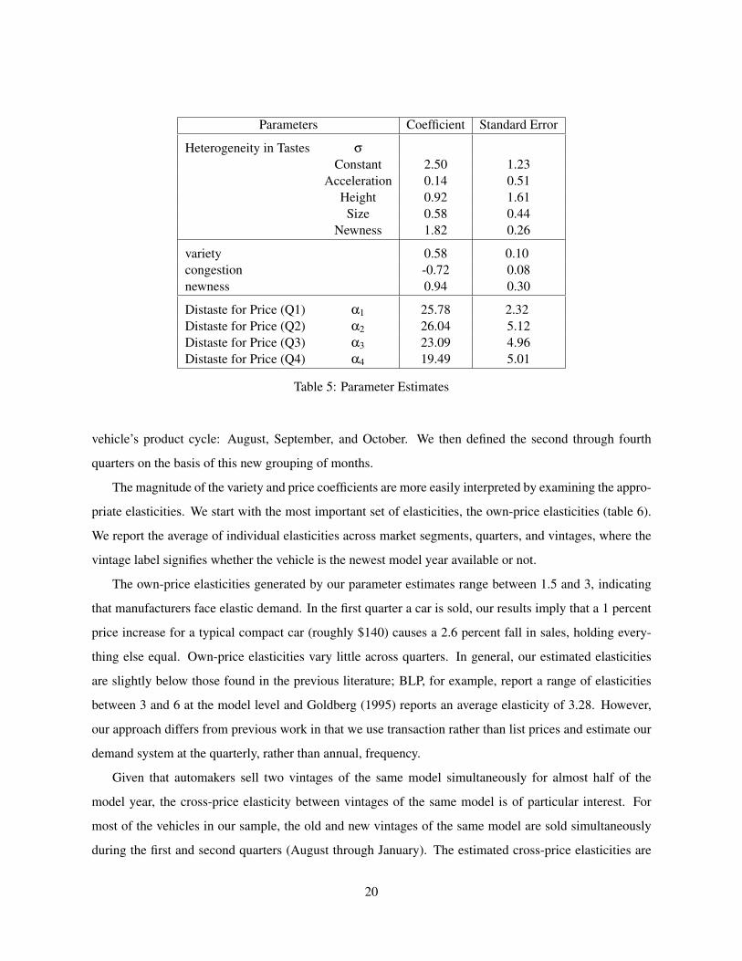
Results: We present a subset of the parameter estimates in table 5. Given their large number, we do not
report all our estimates on the linear portion of utility (β in equation 13). Instead, we show the estimates
of the congestion, variety, and newness coefficients, the consumers’ distaste for price (α) and the measure
of the heterogeneity in consumers’ tastes (σ). The standard errors reported in table 5 have been corrected
for serial correlation of ξ within a vehicle (i.e. a given model/model-year) across quarters.
The coefficients on the acceleration, height and size are not statistically significant. However, we
estimate that consumers are quite heterogeneous in their tastes for purchasing a new car (i.e. the constant
term) and in their tastes for purchasing a new car at the beginning of the model year (i.e. the newness
variable). The positive, significant value of the variety term accords with our prior belief that more variety
is valued by consumers. The magnitude of this coefficient is more easily appreciated in terms of an
elasticity, which is discussed below. The negative and significant value of the congestion term indicates that
congestion is important in the automobile market when considering the overlap in vintages. As detailed
in Ackerberg and Rysman (2005), this result shows the importance for flexibility in the i.i.d. logit errors
across different vintages of the same model. Otherwise, the estimated parameters (especially the price
coefficients) could be biased.
Most importantly, the price coefficients are precisely estimated. The estimated value of households’
distaste for price is in the neighborhood of 25, although there is a drop off in its value in the fourth quarter.
The quarters differ from calendar quarters. We defined the first quarter as the first three months of a typical
of consumers’ indirect utility for our demand-side model.
19
Parameters Coefficient Standard Error
Heterogeneity in Tastes σConstant 2.50 1.23
Acceleration 0.14 0.51Height 0.92 1.61Size 0.58 0.44
Newness 1.82 0.26
variety 0.58 0.10congestion -0.72 0.08newness 0.94 0.30
Distaste for Price (Q1) α1 25.78 2.32Distaste for Price (Q2) α2 26.04 5.12Distaste for Price (Q3) α3 23.09 4.96Distaste for Price (Q4) α4 19.49 5.01
Table 5: Parameter Estimates
vehicle’s product cycle: August, September, and October. We then defined the second through fourth
quarters on the basis of this new grouping of months.
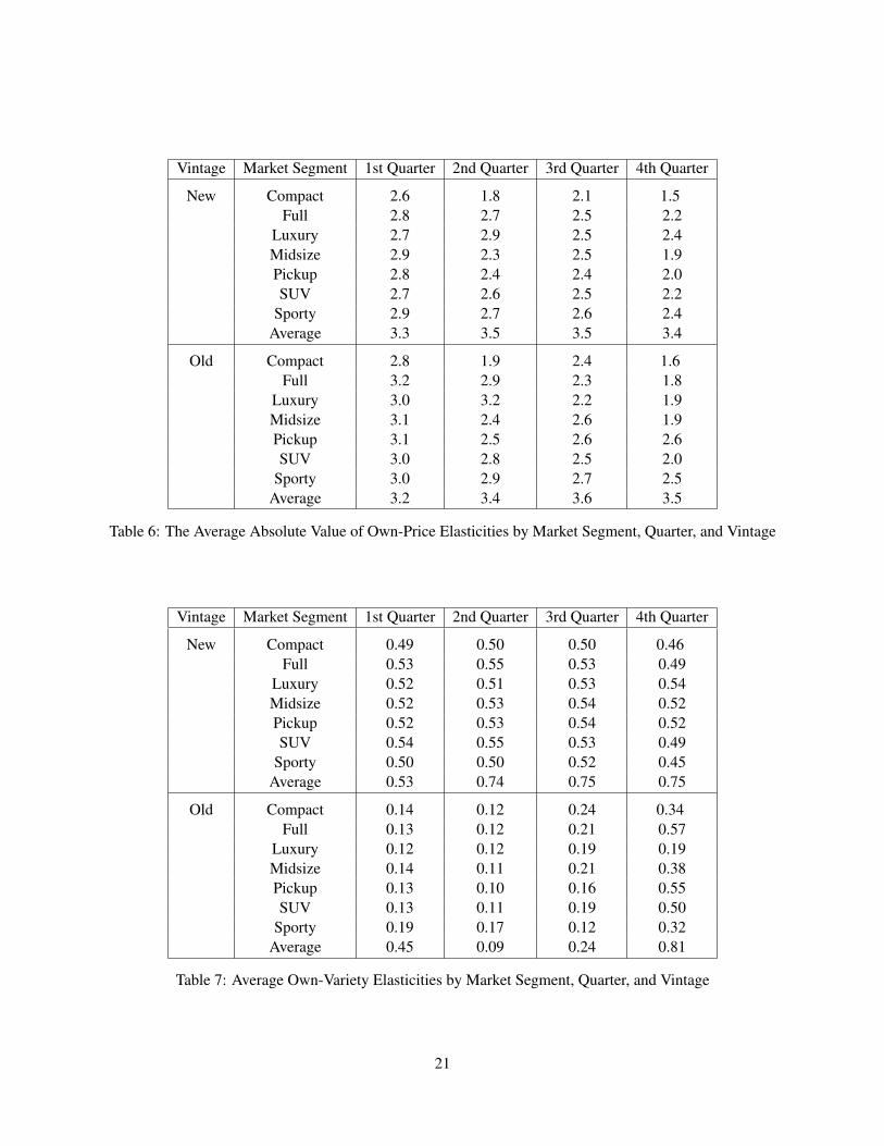
The magnitude of the variety and price coefficients are more easily interpreted by examining the appro-
priate elasticities. We start with the most important set of elasticities, the own-price elasticities (table 6).
We report the average of individual elasticities across market segments, quarters, and vintages, where the
vintage label signifies whether the vehicle is the newest model year available or not.
The own-price elasticities generated by our parameter estimates range between 1.5 and 3, indicating
that manufacturers face elastic demand. In the first quarter a car is sold, our results imply that a 1 percent
price increase for a typical compact car (roughly $140) causes a 2.6 percent fall in sales, holding every-
thing else equal. Own-price elasticities vary little across quarters. In general, our estimated elasticities
are slightly below those found in the previous literature; BLP, for example, report a range of elasticities
between 3 and 6 at the model level and Goldberg (1995) reports an average elasticity of 3.28. However,
our approach differs from previous work in that we use transaction rather than list prices and estimate our
demand system at the quarterly, rather than annual, frequency.
Given that automakers sell two vintages of the same model simultaneously for almost half of the
model year, the cross-price elasticity between vintages of the same model is of particular interest. For
most of the vehicles in our sample, the old and new vintages of the same model are sold simultaneously
during the first and second quarters (August through January). The estimated cross-price elasticities are
20
Vintage Market Segment 1st Quarter 2nd Quarter 3rd Quarter 4th Quarter
New Compact 2.6 1.8 2.1 1.5Full 2.8 2.7 2.5 2.2
Luxury 2.7 2.9 2.5 2.4Midsize 2.9 2.3 2.5 1.9Pickup 2.8 2.4 2.4 2.0SUV 2.7 2.6 2.5 2.2
Sporty 2.9 2.7 2.6 2.4Average 3.3 3.5 3.5 3.4
Old Compact 2.8 1.9 2.4 1.6Full 3.2 2.9 2.3 1.8
Luxury 3.0 3.2 2.2 1.9Midsize 3.1 2.4 2.6 1.9Pickup 3.1 2.5 2.6 2.6SUV 3.0 2.8 2.5 2.0
Sporty 3.0 2.9 2.7 2.5Average 3.2 3.4 3.6 3.5
Table 6: The Average Absolute Value of Own-Price Elasticities by Market Segment, Quarter, and Vintage
Vintage Market Segment 1st Quarter 2nd Quarter 3rd Quarter 4th Quarter
New Compact 0.49 0.50 0.50 0.46Full 0.53 0.55 0.53 0.49
Luxury 0.52 0.51 0.53 0.54Midsize 0.52 0.53 0.54 0.52Pickup 0.52 0.53 0.54 0.52SUV 0.54 0.55 0.53 0.49
Sporty 0.50 0.50 0.52 0.45Average 0.53 0.74 0.75 0.75
Old Compact 0.14 0.12 0.24 0.34Full 0.13 0.12 0.21 0.57
Luxury 0.12 0.12 0.19 0.19Midsize 0.14 0.11 0.21 0.38Pickup 0.13 0.10 0.16 0.55SUV 0.13 0.11 0.19 0.50
Sporty 0.19 0.17 0.12 0.32Average 0.45 0.09 0.24 0.81
Table 7: Average Own-Variety Elasticities by Market Segment, Quarter, and Vintage
21
quite small, ranging from near 0 to 0.02 (see the appendix for detailed numbers); various vintages of the
same model, then, are typically quite imperfect substitutes.17 This result is not intuitive given the often
similar characteristics of different vintages of the same model. Yet, the implication that consumers do
not consider the old and new model-year vintages as close substitutes accords with their dramatic price
differences (recall the 9 percent new vintage premium documented earlier). A possible explanation for
this pricing pattern is price discrimination. By setting prices such that they decline over the model year,
automakers may be separating out eager consumers who are impatient for the latest and greatest vehicle,
from patient consumers who are willing to wait to purchase a new vehicle at the end of the model year.18 In
such an scenario, small price changes would induce little substitution across vintages of the same model.
Finally, we turn to the own-variety elasticities implied by the model. As shown in table 7, variety plays
an important role in consumers’ automobile purchasing decisions. Over the first 4 quarters of the model’s
product life, increases in variety significantly bolster demand. Over this period, a 1 percent increase in
variety bolsters sales by roughly 0.5 percent. The elasticities drop in the fifth and sixth quarter, however,
implying there are only small gains to increasing variety at the end of the model year.
We use these results to parameterize a reduced-form demand curve, equation 1, for each market seg-
ment. Because we are modeling the firm at a weekly frequency, but have quarterly estimates, we interpolate
to create elasticities at the weekly frequency. From our data, we construct a monthly time-series of average
price, quantity, and variety of the new and old vintage by market segment, which we interpolate to produce
a weekly series. For every week, we then solve for the demand curve’s constant term, µ jt , by assuming that
the observed average price-quantity pairs for period t and market segment j, given variety and the com-
peting vintage’s price, is a point on the reduced-form demand curve. The end result are weekly demand
curves for an average vehicle over its life cycle.
An important feature of the resulting sequence of static demand curves is their steady leftward shift
roughly six months after a vehicle has been introduced. This implies that starting half a year into the
product cycle, the firm faces a weakening of demand (i.e. µ jt is decreasing in t) over the remainder of the
product cycle.
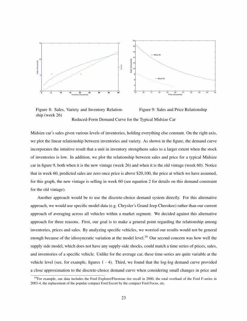
To provide a better sense of inventory’s role in the demand curve, in figure 8 we illustrate a typical17Ana Aizcorbe suggested that geographical factors may explain our low cross-price elasticity estimates. If different vintages
of the same model are rarely offered for sale at the same location, then the degree to which consumers can substitute betweenvintages may be limited.
18Supporting the claim of price discrimination in the new vehicle market, Aizcorbe et al (2007) reports survey data that showsthat incomes of new vehicle purchasers falls by over 8 percent over the automotive model year.
22
0 5 10 15 20 25 30 35 400
5
10
15
Sale
s (th
ousa
nds)
Inventory (thousands)
← →
0 5 10 15 20 25 30 35 400
1
2
Varie
ty
Figure 8: Sales, Variety and Inventory Relation-ship (week 26)
15 16 17 18 19 20 21 22 23 24 252
4
6
8
10
12
14
16
18
20
Sale
s (th
ousa
nds)
Price (thousands)
← Week 26
← Week 60
Figure 9: Sales and Price Relationship
Reduced-Form Demand Curve for the Typical Midsize Car
Midsize car’s sales given various levels of inventories, holding everything else constant. On the right axis,
we plot the linear relationship between inventories and variety. As shown in the figure, the demand curve
incorporates the intuitive result that a unit in inventory strengthens sales to a larger extent when the stock
of inventories is low. In addition, we plot the relationship between sales and price for a typical Midsize
car in figure 9, both when it is the new vintage (week 26) and when it is the old vintage (week 60). Notice
that in week 60, predicted sales are zero once price is above $20,100, the price at which we have assumed,
for this graph, the new vintage is selling in week 60 (see equation 2 for details on this demand constraint
for the old vintage).
Another approach would be to use the discrete-choice demand system directly. For this alternative
approach, we would use specific model data (e.g. Chrysler’s Grand Jeep Cherokee) rather than our current
approach of averaging across all vehicles within a market segment. We decided against this alternative
approach for three reasons. First, our goal is to make a general point regarding the relationship among
inventories, prices and sales. By analyzing specific vehicles, we worried our results would not be general
enough because of the idiosyncratic variation at the model level.19 Our second concern was how well the
supply side model, which does not have any supply-side shocks, could match a time series of prices, sales,
and inventories of a specific vehicle. Unlike for the average car, these time-series are quite variable at the
vehicle level (see, for example, figures 1 - 4). Third, we found that the log-log demand curve provided
a close approximation to the discrete-choice demand curve when considering small changes in price and19For example, our data includes the Ford Explorer/Firestone tire recall in 2000, the total overhaul of the Ford F-series in
2003-4, the replacement of the popular compact Ford Escort by the compact Ford Focus, etc.
23
variety. As shown in the appendix, there are not large differences between each approach’s predicted sales
for a particular model. As such, for the purposes of this paper, there seems to be little cost to employing
the parameterized reduced-form demand curve in place of the discrete-choice demand system.
3.2 Supply-side parameters
To parameterize the cost function, we set the line speed, workers per shift, and wage rates to values
typically observed at assembly plants. The line speed at most North American assembly plants is set
between 35 and 60 cars per hour; thus, we fix the line speed to 45 cars per hour.20 Using the employment
data from Hall (2000), we set n to 1300 workers per shift, so the plant employs 2600 workers. We read the
wages off the union contract: w1 = $27.00 per hour, and w2 = $28.35 per hour. Also based on the union
contract and industry practices, we impose mild seasonality on production assuming that the plant closes
for two weeks in July (weeks 51 and 52) for a model changeover, for a week between Christmas and New
Years Day (week 23), and for single days throughout the year corresponding to traditional holidays.
We set the remaining two parameters, γ and 1/(1 + r), to match for each market segment two first
moments in the data: the average retail price and days-supply. Although we would have preferred to
formally estimate these parameters, the time needed to compute the model’s solution made this infeasible.
The per vehicle material cost, γ, effectively scales the cost function linearly. We set γ between 39.5 percent
(sport) and 63 percent (luxury) of the average retail price to match the observed prices. We choose values
of 1/(1 + r), the weekly discount factor, between 0.962 for pickups to 0.982 for sport cars to match the
average days-supply of inventories observed in the data. These values imply a high degree of impatience
of part of the automaker. A discount factor of 0.975 on $23,000 vehicle implies a weekly holding cost
of $575. At first blush this cost may seem high, but this parameter is the sole cost of holding inventories
and thus it incorporates all the holding costs (e.g. the opportunity cost of funds, physical storage costs,
insurance, physical depreciation, book-keeping costs ...) that are not explicitly modeled. The parameter
values for each market segment are reported in the appendix.
24
Market Sales Days PricesSegment Supply Average Decline Vin. Prem.
Data Model Data Model Data Model Data Model Data Model
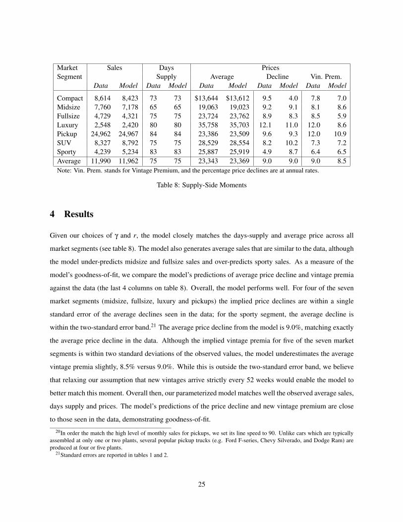
Compact 8,614 8,423 73 73 $13,644 $13,612 9.5 4.0 7.8 7.0Midsize 7,760 7,178 65 65 19,063 19,023 9.2 9.1 8.1 8.6Fullsize 4,729 4,321 75 75 23,724 23,762 8.9 8.3 8.5 5.9Luxury 2,548 2,420 80 80 35,758 35,703 12.1 11.0 12.0 8.6Pickup 24,962 24,967 84 84 23,386 23,509 9.6 9.3 12.0 10.9SUV 8,327 8,792 75 75 28,529 28,554 8.2 10.2 7.3 7.2Sporty 4,239 5,234 83 83 25,887 25,919 4.9 8.7 6.4 6.5Average 11,990 11,962 75 75 23,343 23,369 9.0 9.0 9.0 8.5Note: Vin. Prem. stands for Vintage Premium, and the percentage price declines are at annual rates.
Table 8: Supply-Side Moments
4 Results
Given our choices of γ and r, the model closely matches the days-supply and average price across all
market segments (see table 8). The model also generates average sales that are similar to the data, although
the model under-predicts midsize and fullsize sales and over-predicts sporty sales. As a measure of the
model’s goodness-of-fit, we compare the model’s predictions of average price decline and vintage premia
against the data (the last 4 columns on table 8). Overall, the model performs well. For four of the seven
market segments (midsize, fullsize, luxury and pickups) the implied price declines are within a single
standard error of the average declines seen in the data; for the sporty segment, the average decline is
within the two-standard error band.21 The average price decline from the model is 9.0%, matching exactly
the average price decline in the data. Although the implied vintage premia for five of the seven market
segments is within two standard deviations of the observed values, the model underestimates the average
vintage premia slightly, 8.5% versus 9.0%. While this is outside the two-standard error band, we believe
that relaxing our assumption that new vintages arrive strictly every 52 weeks would enable the model to
better match this moment. Overall then, our parameterized model matches well the observed average sales,
days supply and prices. The model’s predictions of the price decline and new vintage premium are close
to those seen in the data, demonstrating goodness-of-fit.20In order the match the high level of monthly sales for pickups, we set its line speed to 90. Unlike cars which are typically
assembled at only one or two plants, several popular pickup trucks (e.g. Ford F-series, Chevy Silverado, and Dodge Ram) areproduced at four or five plants.
21Standard errors are reported in tables 1 and 2.
25
As a robustness check, we re-solved our model with a higher cross-price elasticity for different vintages
of the same model. Recall our demand side model estimates this cross-price elasticity to be essentially
zero. To determine how important this parameter is to our main results we recomputed table 8 using a
cross-price elasticity of 0.2, holding everything else constant. We chose 0.2 because this value is typically
an upper bound on a vehicle’s cross-price elasticities.22 Reassuringly, our results are robust to the higher
cross-price elasticity parameter (see the appendix for details). Our results are also robust to larger own-
price elasticities; in preliminary work we used own-price elasticities ranging from 6 to 10 and found the
same qualitative results reported in this paper.23
To illustrate the importance of inventories in the model we consider the firm’s pricing decision for a
typical midsize car. Because the automaker faces a downward-sloping demand curve, the profit-maximizing
price sets marginal revenue equal to marginal cost. If we set the cross-price elasticities equal to zero, the
optimal price for this year’s model is
pthist =
−sthist (pt)
∂sthist (pt)/∂pt
+1
1+ rV2(Ilast
t − slastt , Ithis
t +qthist − sthis
t , t +1), (14)
where V2 denotes the derivative of the value function with respect to the second argument. This is the
standard condition for monopoly pricing, but in this case marginal cost is the shadow value of an additional
unit of inventory next period. The opportunity cost of selling a vehicle this week is the inability to sell it
next week. Hence, the shadow values of inventories drives, in large part, the firm’s optimal pricing rule.
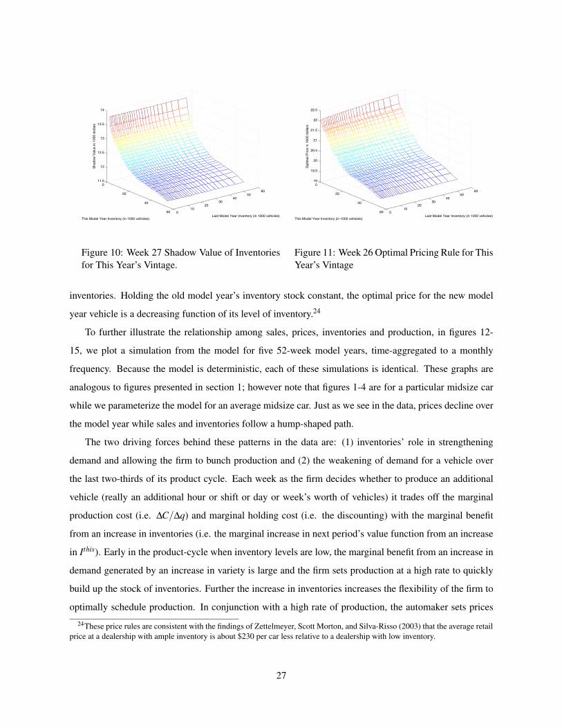
In figure 10, we plot the shadow value of inventories for week 27 (other weeks are qualitatively simi-
lar), at each point in the state space. The shadow value of inventories is a decreasing function of the stock
of inventories, ranging from $13,827 to $11,919. An additional unit of inventory is valuable to the firm
because it increases both the firm’s ability to optimally schedule production and the variety of products
available to consumers. Naturally, however, these benefits are worth less when the firm already has a large
stock of inventories; when the firm holds 50,000 vehicles in stock, our model estimates that the marginal
vehicle in inventory is worth less to the firm than the average cost of producing a vehicle running two
40-hour shifts.
We then plot the pricing rule for this year’s vintage for week 26 in figure 11 for every point in the
state space. As anticipated by equation (14), the pricing rule is almost the shape of the shadow value of22Schiraldi (2010) reports the average cross-price elasticity between vehicles of the same type to be between 0.08 and 0.28.
Schiraldi also reports cross-price elasticities between different vintages of vehicles of the same type, and these elasticities aremuch lower than 0.2.
23In fact, having higher own-price elasticities increased by how much the firm’s inventory management strategy explained theprice declines observed within the model year.
26
0
20
40
60 010
2030
4050
60
11.5
12
12.5
13
13.5
14
Last Model Year Inventory (in 1000 vehicles)This Model Year Inventory (in 1000 vehicles)
Shad
ow V
alue
in 1
000
dolla
rs
Figure 10: Week 27 Shadow Value of Inventoriesfor This Year’s Vintage.
0
20
40
60 010
2030
4050
60
19
19.5
20
20.5
21
21.5
22
22.5
Last Model Year Inventory (in 1000 vehicles)This Model Year Inventory (in 1000 vehicles)
Opt
imal
Pric
e in
100
0 do
llars
Figure 11: Week 26 Optimal Pricing Rule for ThisYear’s Vintage
inventories. Holding the old model year’s inventory stock constant, the optimal price for the new model
year vehicle is a decreasing function of its level of inventory.24
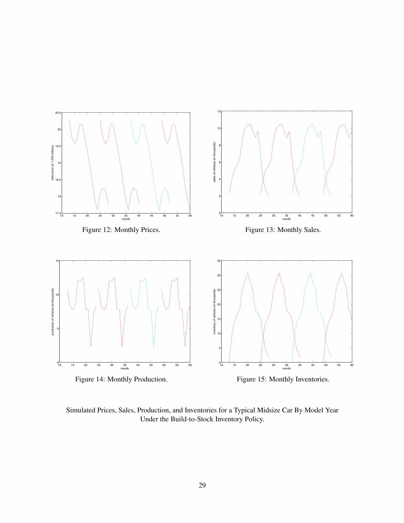
To further illustrate the relationship among sales, prices, inventories and production, in figures 12-
15, we plot a simulation from the model for five 52-week model years, time-aggregated to a monthly
frequency. Because the model is deterministic, each of these simulations is identical. These graphs are
analogous to figures presented in section 1; however note that figures 1-4 are for a particular midsize car
while we parameterize the model for an average midsize car. Just as we see in the data, prices decline over
the model year while sales and inventories follow a hump-shaped path.
The two driving forces behind these patterns in the data are: (1) inventories’ role in strengthening
demand and allowing the firm to bunch production and (2) the weakening of demand for a vehicle over
the last two-thirds of its product cycle. Each week as the firm decides whether to produce an additional
vehicle (really an additional hour or shift or day or week’s worth of vehicles) it trades off the marginal
production cost (i.e. ∆C/∆q) and marginal holding cost (i.e. the discounting) with the marginal benefit
from an increase in inventories (i.e. the marginal increase in next period’s value function from an increase
in Ithis). Early in the product-cycle when inventory levels are low, the marginal benefit from an increase in
demand generated by an increase in variety is large and the firm sets production at a high rate to quickly
build up the stock of inventories. Further the increase in inventories increases the flexibility of the firm to
optimally schedule production. In conjunction with a high rate of production, the automaker sets prices24These price rules are consistent with the findings of Zettelmeyer, Scott Morton, and Silva-Risso (2003) that the average retail
price at a dealership with ample inventory is about $230 per car less relative to a dealership with low inventory.
27
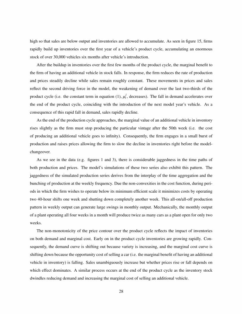
high so that sales are below output and inventories are allowed to accumulate. As seen in figure 15, firms
rapidly build up inventories over the first year of a vehicle’s product cycle, accumulating an enormous
stock of over 30,000 vehicles six months after vehicle’s introduction.
After the buildup in inventories over the first few months of the product cycle, the marginal benefit to
the firm of having an additional vehicle in stock falls. In response, the firm reduces the rate of production
and prices steadily decline while sales remain roughly constant. These movements in prices and sales
reflect the second driving force in the model, the weakening of demand over the last two-thirds of the
product cycle (i.e. the constant term in equation (1), µ jt , decreases). The fall in demand accelerates over
the end of the product cycle, coinciding with the introduction of the next model year’s vehicle. As a
consequence of this rapid fall in demand, sales rapidly decline.
As the end of the production cycle approaches, the marginal value of an additional vehicle in inventory
rises slightly as the firm must stop producing the particular vintage after the 50th week (i.e. the cost
of producing an additional vehicle goes to infinity). Consequently, the firm engages in a small burst of
production and raises prices allowing the firm to slow the decline in inventories right before the model-
changeover.
As we see in the data (e.g. figures 1 and 3), there is considerable jaggedness in the time paths of
both production and prices. The model’s simulations of these two series also exhibit this pattern. The
jaggedness of the simulated production series derives from the interplay of the time aggregation and the
bunching of production at the weekly frequency. Due the non-convexities in the cost function, during peri-
ods in which the firm wishes to operate below its minimum efficient scale it minimizes costs by operating
two 40-hour shifts one week and shutting down completely another week. This all-on/all-off production
pattern in weekly output can generate large swings in monthly output. Mechanically, the monthly output
of a plant operating all four weeks in a month will produce twice as many cars as a plant open for only two
weeks.
The non-monotonicity of the price contour over the product cycle reflects the impact of inventories
on both demand and marginal cost. Early on in the product cycle inventories are growing rapidly. Con-
sequently, the demand curve is shifting out because variety is increasing, and the marginal cost curve is
shifting down because the opportunity cost of selling a car (i.e. the marginal benefit of having an additional
vehicle in inventory) is falling. Sales unambiguously increase but whether prices rise or fall depends on
which effect dominates. A similar process occurs at the end of the product cycle as the inventory stock
dwindles reducing demand and increasing the marginal cost of selling an additional vehicle.
28
10 15 20 25 30 35 40 45 50 55 6017.5
18
18.5
19
19.5
20
20.5
month
reta
il pric
e (in
1,0
00 d
olla
rs)
Figure 12: Monthly Prices.
10 15 20 25 30 35 40 45 50 55 600
2
4
6
8
10
12
monthsa
les
of v
ehicl
es (i
n th
ousa
nds)
Figure 13: Monthly Sales.
10 15 20 25 30 35 40 45 50 55 600
5
10
15
month
prod
uctio
n of
veh
icles
(in
thou
sand
s)
Figure 14: Monthly Production.
10 15 20 25 30 35 40 45 50 55 600
5
10
15
20
25
30
35
month
inve
ntor
y of
veh
icles
(in
thou
sand
s)
Figure 15: Monthly Inventories.
Simulated Prices, Sales, Production, and Inventories for a Typical Midsize Car By Model YearUnder the Build-to-Stock Inventory Policy.
29
5 The Counterfactual
To better understand the importance of inventories in stimulating demand, we employ the following coun-
terfactual. We re-solve the model setting the variety term in the demand curve (equation 1) to 1.25 for all
104 weeks, turning off inventory’s effect on demand. For a typical vehicle, variety peaks a at little above
1.25, midway through the product cycle. Although sales still can only be made from beginning-of-period
inventories, (equation (3)), we interpret this simulation as approximating a “build-to-order” inventory pol-
icy in which consumers can purchase a vehicle with the exact specification they want. Hence, we assume
that firms can offer consumers “full variety” throughout the product cycle without holding large levels of
inventories. In this case, inventories only serve to facilitate the manufacturer’s cost minimizing produc-
tion schedule and allow the firm to sell the current vintage beyond the twelve month production period.
This contrasts to the “build-to-stock” inventory management strategy firms currently use, where dealer
inventories also provide variety, thereby helping match consumers to their ideal vehicle.
The counterfactual illustrates the importance of the variety-increasing role for inventories. Without
this effect, firms hold much less inventory; the average ratio of inventories to sales is one-fifth the level
compared to the build-to-stock case (see table 9).25 Inventories are now primarily used to lengthen the
sales period of a car. Without the additional benefit from shifting demand, for most of the product cycle,
the marginal value of an additional unit of inventory above one week’s worth of sales does not exceed
its cost of production. Hence, the firm sets the rate of production roughly equal to sales, and these two
series track each other closely with little growth in the level of inventories. Just as in the build-to-stock
case, as the end of the production cycle nears, the firm ratchets up output slightly and increases prices
(thus dampening sales) to accumulate a modest amount of inventory to sell during the first weeks of the
following model year.26
At the same time, the firm temporarily raises prices, damping sales, and so inducing a spike in in-
ventories (see figure 19). Figures 12 and 16 illustrate that prices decline a bit more than half as much
as those observed under the build-to-stock case. The change in pricing strategy reflects the fact that the25As is well-understood in the inventory literature, it is difficult to match the high level of inventories observed in many
industries only relying on inventory’s role in minimizing production costs (e.g. Bils and Kahn, 2000).26The time path of production is less jagged in the build-to-order case (figure 18) than in the build-to-stock case (figure 14).
In both cases, the firm engages in weeklong shutdowns when desired production is less than the MES. However in this particularbuild-to-order simulation, during the first couple of months while desired production is below the MES, productions follows afour-to-five week cycle which is averaged out through the time aggregation. In the build-to-stock case there is less periodicity inthe shutdowns and more overtime hours are employed when the plant is operating, hence the jaggedness in the weekly data is noteliminated, but magnified, with time aggregation.
30
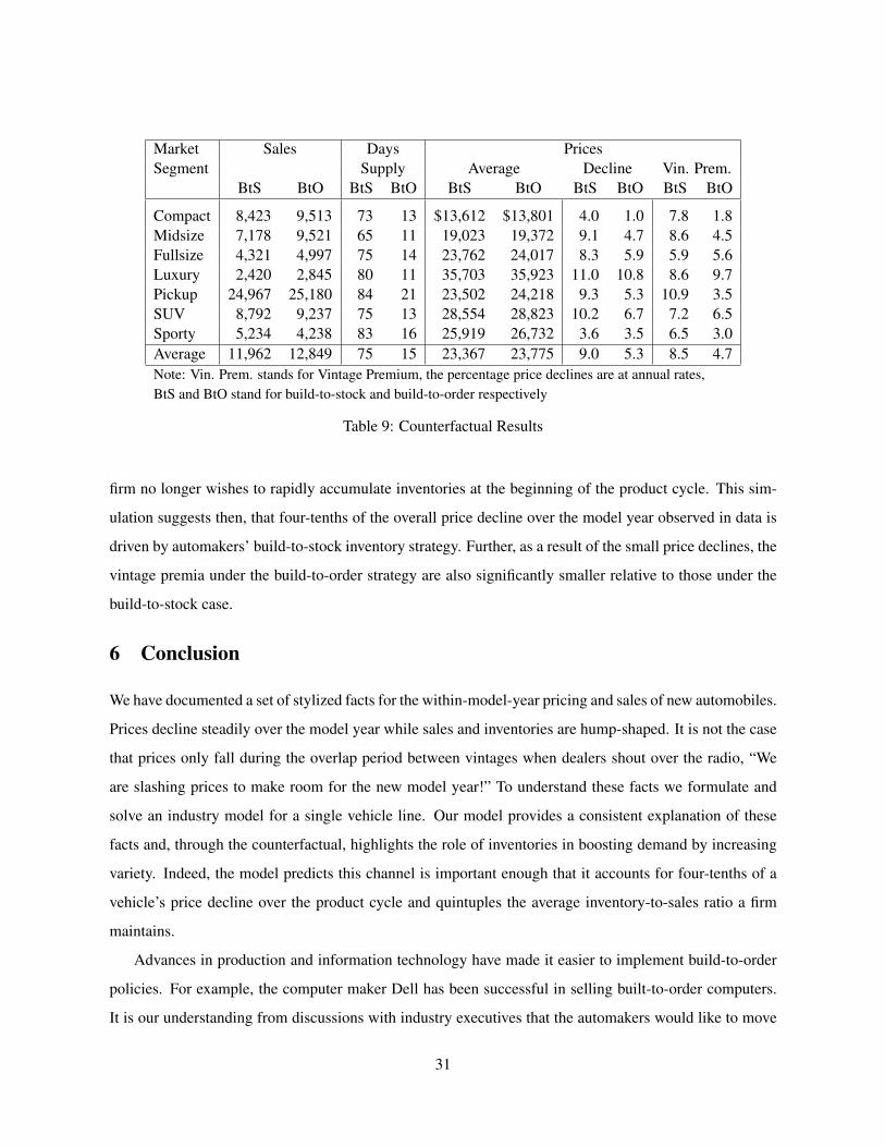
Market Sales Days PricesSegment Supply Average Decline Vin. Prem.
BtS BtO BtS BtO BtS BtO BtS BtO BtS BtO
Compact 8,423 9,513 73 13 $13,612 $13,801 4.0 1.0 7.8 1.8Midsize 7,178 9,521 65 11 19,023 19,372 9.1 4.7 8.6 4.5Fullsize 4,321 4,997 75 14 23,762 24,017 8.3 5.9 5.9 5.6Luxury 2,420 2,845 80 11 35,703 35,923 11.0 10.8 8.6 9.7Pickup 24,967 25,180 84 21 23,502 24,218 9.3 5.3 10.9 3.5SUV 8,792 9,237 75 13 28,554 28,823 10.2 6.7 7.2 6.5Sporty 5,234 4,238 83 16 25,919 26,732 3.6 3.5 6.5 3.0Average 11,962 12,849 75 15 23,367 23,775 9.0 5.3 8.5 4.7Note: Vin. Prem. stands for Vintage Premium, the percentage price declines are at annual rates,BtS and BtO stand for build-to-stock and build-to-order respectively
Table 9: Counterfactual Results
firm no longer wishes to rapidly accumulate inventories at the beginning of the product cycle. This sim-
ulation suggests then, that four-tenths of the overall price decline over the model year observed in data is
driven by automakers’ build-to-stock inventory strategy. Further, as a result of the small price declines, the
vintage premia under the build-to-order strategy are also significantly smaller relative to those under the
build-to-stock case.
6 Conclusion
We have documented a set of stylized facts for the within-model-year pricing and sales of new automobiles.
Prices decline steadily over the model year while sales and inventories are hump-shaped. It is not the case
that prices only fall during the overlap period between vintages when dealers shout over the radio, “We
are slashing prices to make room for the new model year!” To understand these facts we formulate and
solve an industry model for a single vehicle line. Our model provides a consistent explanation of these
facts and, through the counterfactual, highlights the role of inventories in boosting demand by increasing
variety. Indeed, the model predicts this channel is important enough that it accounts for four-tenths of a
vehicle’s price decline over the product cycle and quintuples the average inventory-to-sales ratio a firm
maintains.
Advances in production and information technology have made it easier to implement build-to-order
policies. For example, the computer maker Dell has been successful in selling built-to-order computers.
It is our understanding from discussions with industry executives that the automakers would like to move
31
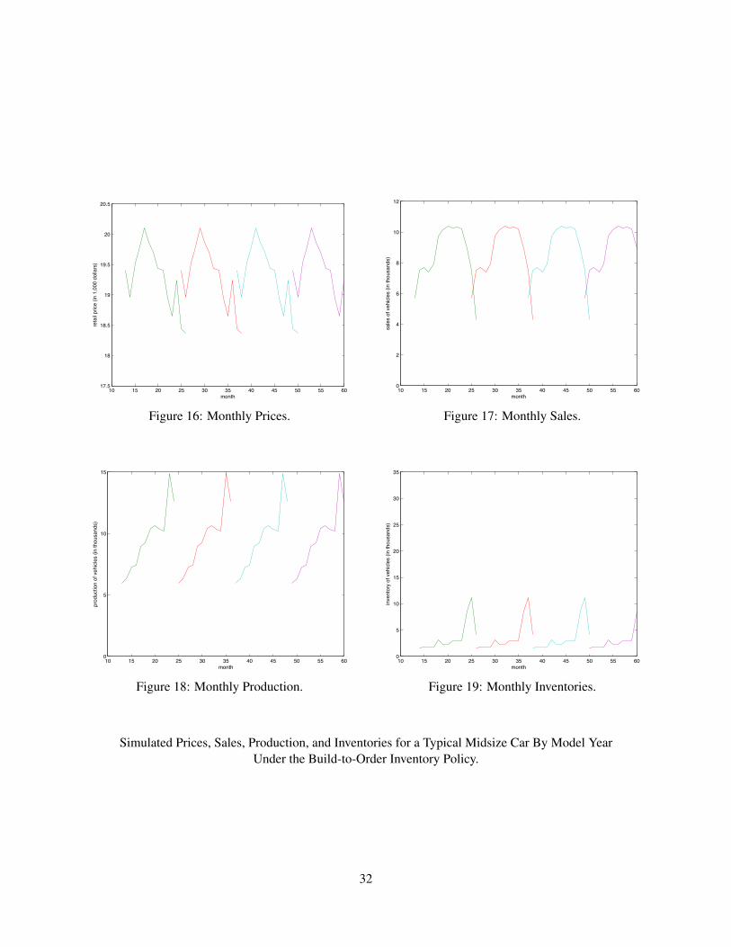
10 15 20 25 30 35 40 45 50 55 6017.5
18
18.5
19
19.5
20
20.5
month
reta
il pric
e (in
1,0
00 d
olla
rs)
Figure 16: Monthly Prices.
10 15 20 25 30 35 40 45 50 55 600
2
4
6
8
10
12
monthsa
les
of v
ehicl
es (i
n th
ousa
nds)
Figure 17: Monthly Sales.
10 15 20 25 30 35 40 45 50 55 600
5
10
15
month
prod
uctio
n of
veh
icles
(in
thou
sand
s)
Figure 18: Monthly Production.
10 15 20 25 30 35 40 45 50 55 600
5
10
15
20
25
30
35
month
inve
ntor
y of
veh
icles
(in
thou
sand
s)
Figure 19: Monthly Inventories.
Simulated Prices, Sales, Production, and Inventories for a Typical Midsize Car By Model YearUnder the Build-to-Order Inventory Policy.
32
toward an inventory policy in which a larger fraction of consumers order their new vehicles rather than
buy whatever is on the dealer’s lot. Our analysis suggests that enacting such a policy will damp the within-
model-year price declines and reduce the period in which consecutive vintages compete with each other.
A shortcoming of this paper is the use of static demand. While it is difficult to predict the impact of
using a dynamic demand model on our results, we conjecture that our main results would remain qualita-
tively the same. Based on the marketing literature, Keane (2010) (see page 52 and footnote 8) claims that
dynamic demand models typically produce lower price elasticities relative to static models. A change in
the price elasticities should not be problematic, however, since our robustness checks show that our main
results hold for a range of elasticity estimates. Of course, solving the dynamic firm’s problem when faced
with a dynamic demand system which allows for intertemporal substitution may produce unexpected re-
sults. Incorporating dynamic demand would be particularly insightful, since we could compute how much
of the observed within model-year price declines for automobiles is due to intertemporal price discrimina-
tion, inventory management, and other forces. It’s possible that our main result that automakers’ inventory
management accounts for four-tenths of the price decline would be greatly diminished given dynamic de-
mand. Given the results from the inventory literature, however, we find this unlikely. As mentioned in
our literature review, the macro-inventory literature finds that inventory’s role in smoothing production is
simply not enough to explain the high levels of automobiles held in inventory. Hence, in order to match
the inventory levels observed in the data, this literature has relied on ad hoc assumptions that inventories
play a role in generating sales. Reassuringly, this channel is supported by the industry wisdom that putting
more cars on automobile dealers’ lots (i.e. building up inventories) is believed to generate more sales by
better matching consumers to their ideal vehicle. Consequently, we find it unlikely that a richer model in-
corporating dynamic demand would wipe out a role for inventories in generating sales. Given inventory’s
role in generating sales, our model predicts that the firm’s inventory management policy will drive part of
the within model-year price declines observed in the data.
33
References
[1] Aizcorbe, A., Kortum, S. 2005. Moore’s Law and the semiconductor industry: A vintage model.
Scandinavian Journal of Economics 107, 603-630.
[2] Aizcorbe, A., Bridgman, B., Nalewaik J. 2007. The implications of heterogeneous buyers for mea-
suring quality change. manuscript, Bureau of Economic Analysis.
[3] Ayres, I., Siegelman P., 1995. Race and gender discrimination in bargaining for a new car. American
Economic Review 85, 304-321.
[4] Ackerberg, D., Rysman, M. 2005. Unobserved product differentiaion in discrete-choice models: es-
timating price elasticities and welfare effects. Rand Journal of Economics 36, 771-788.
[5] Aguirregabiria, V., 1999. The Dynamics of Markups and Inventories in Retailing Firms. The Review
of Economic Studies, 66, 275-308.
[6] Berry, S., 1994. Estimating discrete-choice models of product differentiation. Rand Journal of Eco-
nomics 25, 242-261.
[7] Berry, S., Levinsohn J., Pakes A., 1995. Automobile prices in market equilibrium. Econometrica 63,
841-890.
[8] Berry, S., Levinsohn J., Pakes A., 1999. Voluntary export restraints on automobiles: Evaluating a
trade policy. American Economic Review 89, 400-430.
[9] Bils, M., Kahn J. 2000. What inventory behavior tells us about business cycles. American Economic
Review 90, 458-481.
[10] Blanchard O., 1983. The production and inventory behavior of the American automobile Industry.
Journal of Political Economy 91, 365-400.
[11] Bresnahan, T., Reiss, P., 1985. Dealer and manufacter margins. Rand Journal of Economics 16, 253-
268.
[12] Bresnahan, T., Ramey, V., 1994. Output fluctuations at the plant level. Quarterly Journal of Eco-
nomics 109, 593-624.
34
[13] Busse, M., Silva-Risso, J., Zettlemeyer, F., 2006. $1000 cash back: The pass-through of auto manu-
facturer promotions. American Economic Review 96, 1253-1270.
[14] Cachon, G.P., Olivares, M., 2008. Drivers of finished goods inventory in the U.S. automobile industry,
SSRN working paper.
[15] Chevalier, J., Goolsbee A., 2007. Are durable good consumers forward looking? Evidence from the
college textbook market, manuscript, Yale University.
[16] Conlisk, J., Gerstner, E., Sobel. J., 1984. Cyclic pricing by a durable goods monopolist. Quarterly
Journal of Economics 99, 489-505.
[17] Corrado, C., Dunn, W., Otoo M., 2004. An initial look at incentives and prices for motor vehicles:
What has been happening in recent years? manuscript, Board of Governors of the Federal Reserve.
[18] Copeland, A., Hall, G., forthcoming. The response of prices, sales, and output to temporary changes
in demand. Journal of Applied Econometrics.
[19] Copeland, A., Shapiro, A., 2009. The impact of competition on technology adoption: An Apples-to-
PCs analysis. manuscript, Federal Reserve Bank of New York.
[20] Elmaghraby W., Keskinocak P. 2003. Dynamic pricing in the presence of inventory considerations:
Research overview, current practices, and future directions. Managment Science 49, 1287-1309.
[21] Federgruen, A., Heching A.,1999. Combined pricing and inventory control under uncertainty. Oper-
ations Research 47, 454-475.
[22] Goldberg, P., 1995. Product differentiation and oliogopoly in international markets: The case of the
U.S. automobile industry. Econometrica 63, 891-951.
[23] Goldberg, P., 1996. Dealer price discrimination in new car purchases: Evidence from the consumer
expenditure survey. Journal of Political Economy 104, 622-654.
[24] Gowrisankaran, G., Rysman, M., 2007. Dynamics of consumer demand for new durable goods.
manuscript, University of Arizona.
[25] Hall G., 2000. Non-convex costs and capital utilization: A study of production scheduling at auto-
mobile assembly plants. Journal of Monetary Economics 45, 681-716.
35
[26] Hamermesh D., 1989. Labor demand and the structure of adjustment costs. American Economic
Review 79, 674-689.
[27] Kahn J., 1987. Inventories and the volatility of production. American Economic Review 77(4), 667-
679.
[28] Kahn J., 1992. Why is production more volatile than sales? Theory and evidence on the stockout-
avoidance motive for inventory-holding. Quarterly Journal of Economics 109(3), 565-592.
[29] Karlin, S., Carr R., 1962. Prices and optimal inventory policy. in Studies in Applied Probability and
Management Science, K. Arrow, S. Karlin, H. Scarf (ed.), Stanford, CA: Stanford University Press.
[30] Keane, M. 2010. A Structural Perspective on the Experimentalist School. Journal of Economic Per-
spectives 24(2), 47-58.
[31] Langer, A. 2009. Demographic Preferences and Price Discrimination in New Vehicle Sales. Univer-
sity of Michigan manuscript.
[32] Lazear, E., 1986. Retail pricing and clearence sales. American Economic Review 76, 14-31.
[33] Nevo, A., 2000. A practitioner’s guide to estimation of random coefficients logit models of demand.
Journal of Economics & Management Strategy 9, 513-548.
[34] Nevo, A., 2001. Measuring market power in the ready-to-eat cereal industry. Econometrica, 69(2),
307-342.
[35] Pashigian, P., 1988. Demand uncertainty and sales: A study of fashion and markdown pricing. Amer-
ican Economic Review 78, 936-953.
[36] Pashigian, P., Bowen B., Gould E., 1995. Fashion, styling, and the within season decline in automo-
bile prices. Journal of Law and Economics 38, 281-310.
[37] Pesendorfer, W., 1995. Design innovation and fashion cycles. American Economic Review 85, 771-
792.
[38] Petrin, A., 2002. Quantifying the benefits of new products: The case of the minivan. Journal of
Political Economy 110, 705-729. American Economic Review 96, 1876-1889.
36
[39] Reagan, P., 1982. Inventory and price behavior. Review of Economic Studies 49, 137-142.
[40] Schiraldi, P., 2010. Automobile replacement: A dynamic structural approach. manuscript, London
School of Economics.
[41] Scott Morton F., Zettelmeyer, F., Silva-Risso J., 2003. Consumer information and discrimination:
Does the internet affect the pricing of new cars to women and minorities? Quantitative marketing
and Economics 1, 65-92.
[42] Stokey, N., 1979. Intertemporal price discrimination. Quarterly Journal of Economics 93, 355-371.
[43] Whiten, T., 1955. Inventory control and price theory. Managment Science 2, 61-80.
[44] Zettelmeyer, F., Scott Morton F., Silva-Risso J., 2003. Inventory fluctuations and price discrimina-
tion: The determinants of price variation in car retailing. manuscript, Yale School of Management.
37
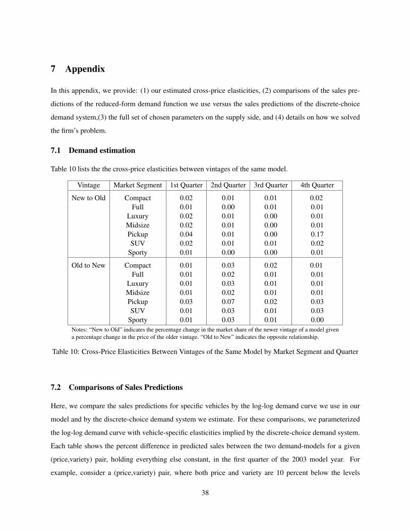
7 Appendix
In this appendix, we provide: (1) our estimated cross-price elasticities, (2) comparisons of the sales pre-
dictions of the reduced-form demand function we use versus the sales predictions of the discrete-choice
demand system,(3) the full set of chosen parameters on the supply side, and (4) details on how we solved
the firm’s problem.
7.1 Demand estimation
Table 10 lists the the cross-price elasticities between vintages of the same model.
Vintage Market Segment 1st Quarter 2nd Quarter 3rd Quarter 4th Quarter
New to Old Compact 0.02 0.01 0.01 0.02Full 0.01 0.00 0.01 0.01
Luxury 0.02 0.01 0.00 0.01Midsize 0.02 0.01 0.00 0.01Pickup 0.04 0.01 0.00 0.17SUV 0.02 0.01 0.01 0.02
Sporty 0.01 0.00 0.00 0.01
Old to New Compact 0.01 0.03 0.02 0.01Full 0.01 0.02 0.01 0.01
Luxury 0.01 0.03 0.01 0.01Midsize 0.01 0.02 0.01 0.01Pickup 0.03 0.07 0.02 0.03SUV 0.01 0.03 0.01 0.03
Sporty 0.01 0.03 0.01 0.00Notes: “New to Old” indicates the percentage change in the market share of the newer vintage of a model givena percentage change in the price of the older vintage. “Old to New” indicates the opposite relationship.
Table 10: Cross-Price Elasticities Between Vintages of the Same Model by Market Segment and Quarter
7.2 Comparisons of Sales Predictions
Here, we compare the sales predictions for specific vehicles by the log-log demand curve we use in our
model and by the discrete-choice demand system we estimate. For these comparisons, we parameterized
the log-log demand curve with vehicle-specific elasticities implied by the discrete-choice demand system.
Each table shows the percent difference in predicted sales between the two demand-models for a given
(price,variety) pair, holding everything else constant, in the first quarter of the 2003 model year. For
example, consider a (price,variety) pair, where both price and variety are 10 percent below the levels
38
observed in the data. For the compact car, the difference in predicted sales is -2.8 percent. Reassuringly,
the tables below demonstrate that the log-log demand curve sales predictions are fairly close to those from
the discrete-choice demand system.
7.3 Supply-side parameters
Table 14 lists the per-vehicle material cost parameter, γ, and discount rate 11+r , for each market segment.
7.4 Solving the firm’s problem
Because of the non-convexities in the cost function, we solve for both the optimal level of output and
the cost minimizing production schedule through grid search. We allow weekly production, q, to take on
values between 0 and 6000 in increments of 50. The grids for Dt and St are set from 1 to 6 and from 0 to
2, respectively, in increments of 1. The plant is closed for the week whenever St = 0. The shift length, ht ,
can take on values of 7, 8, 9 or 10. So there are up to 72 feasible production schedules to evaluate for each
121 possible levels of production.
We discretize each inventory grid into 28 points from 0 to 2.25 times the mean monthly inventory
stock. The distance between grid points increases with the level of inventories. Thus, the grid points
are more densely spaced in the region where the value function has more curvature. For each of the 784
inventory pairs, we maximize the right hand side of equations (10) and (11) over each sales price and level
of output. Points off the two inventory grids are approximated using bi-linear interpolation.
7.5 Robustness tables
In this section we report the results from our robustness exercise. We re-solved the model assuming a
new cross-price elasticity parameter of 0.2 between vintages of the same model, and keeping all other
parameters the same. With this new elasticity, the model continues to match the moments in the data quite
well (see table 15). Furthermore, the results from our counterfactual exercise are robust to this elasticity
change (see table 16).
39
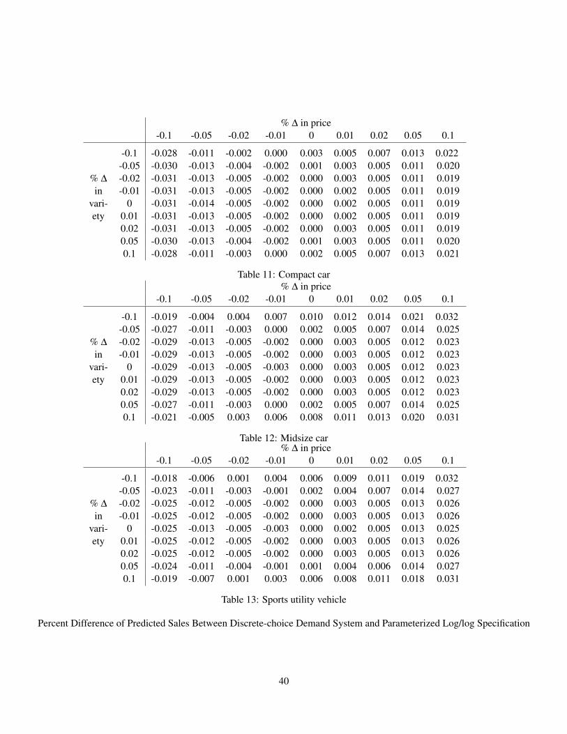
% ∆ in price-0.1 -0.05 -0.02 -0.01 0 0.01 0.02 0.05 0.1
-0.1 -0.028 -0.011 -0.002 0.000 0.003 0.005 0.007 0.013 0.022-0.05 -0.030 -0.013 -0.004 -0.002 0.001 0.003 0.005 0.011 0.020
% ∆ -0.02 -0.031 -0.013 -0.005 -0.002 0.000 0.003 0.005 0.011 0.019in -0.01 -0.031 -0.013 -0.005 -0.002 0.000 0.002 0.005 0.011 0.019
vari- 0 -0.031 -0.014 -0.005 -0.002 0.000 0.002 0.005 0.011 0.019ety 0.01 -0.031 -0.013 -0.005 -0.002 0.000 0.002 0.005 0.011 0.019
0.02 -0.031 -0.013 -0.005 -0.002 0.000 0.003 0.005 0.011 0.0190.05 -0.030 -0.013 -0.004 -0.002 0.001 0.003 0.005 0.011 0.0200.1 -0.028 -0.011 -0.003 0.000 0.002 0.005 0.007 0.013 0.021
Table 11: Compact car% ∆ in price
-0.1 -0.05 -0.02 -0.01 0 0.01 0.02 0.05 0.1
-0.1 -0.019 -0.004 0.004 0.007 0.010 0.012 0.014 0.021 0.032-0.05 -0.027 -0.011 -0.003 0.000 0.002 0.005 0.007 0.014 0.025
% ∆ -0.02 -0.029 -0.013 -0.005 -0.002 0.000 0.003 0.005 0.012 0.023in -0.01 -0.029 -0.013 -0.005 -0.002 0.000 0.003 0.005 0.012 0.023
vari- 0 -0.029 -0.013 -0.005 -0.003 0.000 0.003 0.005 0.012 0.023ety 0.01 -0.029 -0.013 -0.005 -0.002 0.000 0.003 0.005 0.012 0.023
0.02 -0.029 -0.013 -0.005 -0.002 0.000 0.003 0.005 0.012 0.0230.05 -0.027 -0.011 -0.003 0.000 0.002 0.005 0.007 0.014 0.0250.1 -0.021 -0.005 0.003 0.006 0.008 0.011 0.013 0.020 0.031
Table 12: Midsize car% ∆ in price
-0.1 -0.05 -0.02 -0.01 0 0.01 0.02 0.05 0.1
-0.1 -0.018 -0.006 0.001 0.004 0.006 0.009 0.011 0.019 0.032-0.05 -0.023 -0.011 -0.003 -0.001 0.002 0.004 0.007 0.014 0.027
% ∆ -0.02 -0.025 -0.012 -0.005 -0.002 0.000 0.003 0.005 0.013 0.026in -0.01 -0.025 -0.012 -0.005 -0.002 0.000 0.003 0.005 0.013 0.026
vari- 0 -0.025 -0.013 -0.005 -0.003 0.000 0.002 0.005 0.013 0.025ety 0.01 -0.025 -0.012 -0.005 -0.002 0.000 0.003 0.005 0.013 0.026
0.02 -0.025 -0.012 -0.005 -0.002 0.000 0.003 0.005 0.013 0.0260.05 -0.024 -0.011 -0.004 -0.001 0.001 0.004 0.006 0.014 0.0270.1 -0.019 -0.007 0.001 0.003 0.006 0.008 0.011 0.018 0.031
Table 13: Sports utility vehicle
Percent Difference of Predicted Sales Between Discrete-choice Demand System and Parameterized Log/log Specification
40
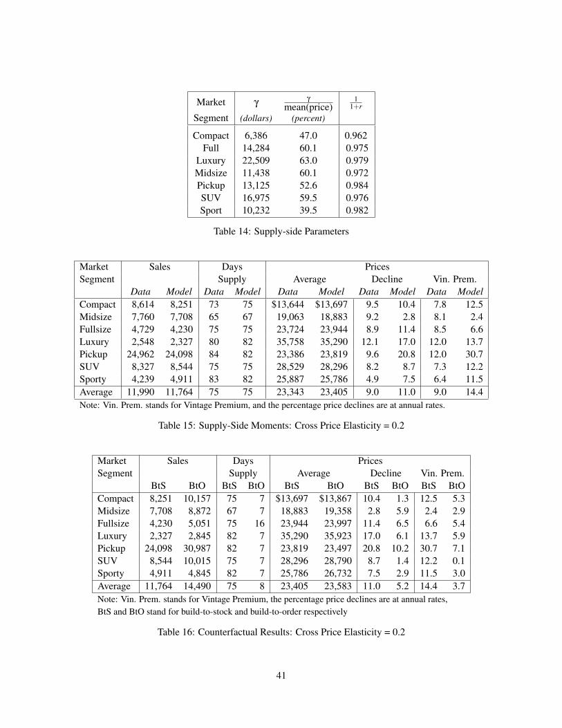
Market γ γmean(price)
11+r
Segment (dollars) (percent)
Compact 6,386 47.0 0.962Full 14,284 60.1 0.975
Luxury 22,509 63.0 0.979Midsize 11,438 60.1 0.972Pickup 13,125 52.6 0.984SUV 16,975 59.5 0.976Sport 10,232 39.5 0.982
Table 14: Supply-side Parameters
Market Sales Days PricesSegment Supply Average Decline Vin. Prem.
Data Model Data Model Data Model Data Model Data ModelCompact 8,614 8,251 73 75 $13,644 $13,697 9.5 10.4 7.8 12.5Midsize 7,760 7,708 65 67 19,063 18,883 9.2 2.8 8.1 2.4Fullsize 4,729 4,230 75 75 23,724 23,944 8.9 11.4 8.5 6.6Luxury 2,548 2,327 80 82 35,758 35,290 12.1 17.0 12.0 13.7Pickup 24,962 24,098 84 82 23,386 23,819 9.6 20.8 12.0 30.7SUV 8,327 8,544 75 75 28,529 28,296 8.2 8.7 7.3 12.2Sporty 4,239 4,911 83 82 25,887 25,786 4.9 7.5 6.4 11.5Average 11,990 11,764 75 75 23,343 23,405 9.0 11.0 9.0 14.4Note: Vin. Prem. stands for Vintage Premium, and the percentage price declines are at annual rates.
Table 15: Supply-Side Moments: Cross Price Elasticity = 0.2
Market Sales Days PricesSegment Supply Average Decline Vin. Prem.
BtS BtO BtS BtO BtS BtO BtS BtO BtS BtOCompact 8,251 10,157 75 7 $13,697 $13,867 10.4 1.3 12.5 5.3Midsize 7,708 8,872 67 7 18,883 19,358 2.8 5.9 2.4 2.9Fullsize 4,230 5,051 75 16 23,944 23,997 11.4 6.5 6.6 5.4Luxury 2,327 2,845 82 7 35,290 35,923 17.0 6.1 13.7 5.9Pickup 24,098 30,987 82 7 23,819 23,497 20.8 10.2 30.7 7.1SUV 8,544 10,015 75 7 28,296 28,790 8.7 1.4 12.2 0.1Sporty 4,911 4,845 82 7 25,786 26,732 7.5 2.9 11.5 3.0Average 11,764 14,490 75 8 23,405 23,583 11.0 5.2 14.4 3.7Note: Vin. Prem. stands for Vintage Premium, the percentage price declines are at annual rates,BtS and BtO stand for build-to-stock and build-to-order respectively
Table 16: Counterfactual Results: Cross Price Elasticity = 0.2
41