�

�

�

�

Invariant preserving integrators :

An algebraic approach

P. Chartier, IPSO, INRIA-RENNES

With the contributions of E. Faou, E. Hairer, A. Murua and

G. Vilmart for some of the recent results

1

�

�

�

�

Qualitative properties of y = f(y)

There are many situations where the differential system

has structural properties that owed to be preserved :

1. First integral : ddtI(y) = 0.

2. Symplectic structure (Hamiltonian systems :

f(y) = J−1∇H(y) ).

3. Symmetry : ρ(f(y)) = −f(ρ(y)).

2

�

�

�

�

Trajectories of 2-D Kepler with various methods

FIG. 1 – E. Hairer, Geometric Integration, pp. 5

3

�

�

�

�

Energy conservation - Global Error

FIG. 2 – E. Hairer, Geometric Integration, pp. 6

4

�

�

�

�

Geometric numerical integration

The main objective of GNI is to study existing numerical integrators and design new

ones that preserve some or all of these properties, with applications to

– celestial mechanics,

– robotics,

– molecular simulation...,

where obtaining an accurate approximation over long integration intervals is out of

reach.

The main idea of GNI is to re-interpret the numerical method as the exact solution of

a modified equation whose qualitative features can be described.

5

�

�

�

�

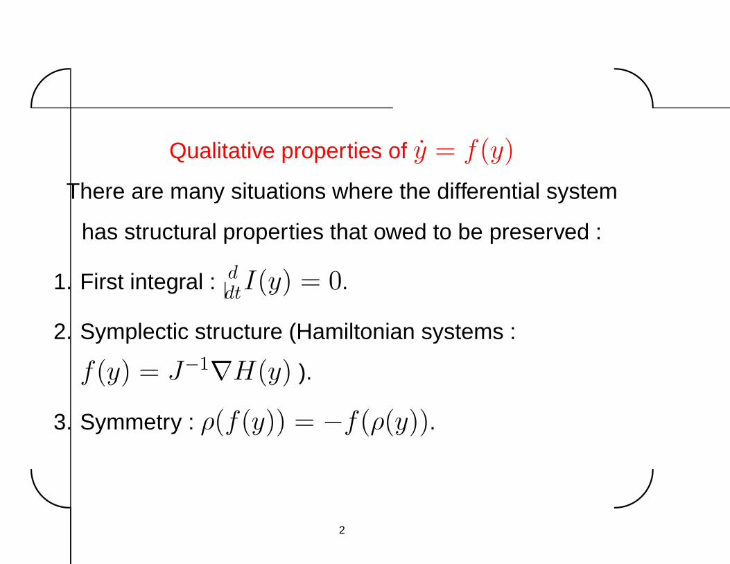
Modified equations

modified problem

⎧⎨⎩

˙y = f(y)

y(0) = y0

↘ exact solution : y(nh) = yn

yn+1 = Φfh(yn)

↗ numerical solution : yn ≈ y(nh)

initial problem

⎧⎨⎩

y = f(y)

y(0) = y0

Strictly speaking, this diagram holds true only formally : its validity can be justified by

a rigorous study of error terms (optimal truncature of the series involved leads to

exponentially small errors).

6

�

�

�

�

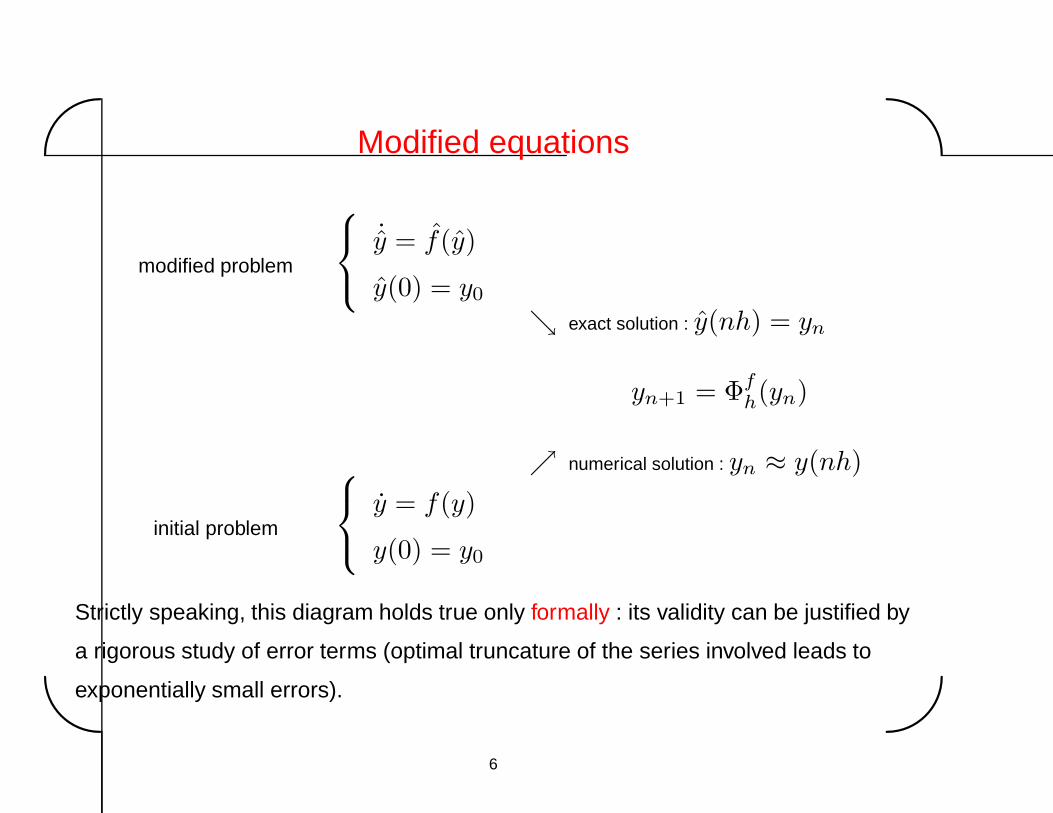
Taylor expansions or the urgent necessity of trees

In trying to get the Taylor expansion of the implicit Euler solution

y1 = y0 + hf(y1)

one gets successively (where we have omitted the argument y0 in f , f ′, ...)

y1 = y0 + h f︸︷︷︸=y′

+O(h2),

y1 = y0 + h f︸︷︷︸=y′

+h2 f ′f︸︷︷︸=y′′

+O(h3),

y1 = y0 + h f︸︷︷︸=y′

+h2 f ′f︸︷︷︸=y′′

+h3(

f ′f ′f +12f ′′(f, f

)︸ ︷︷ ︸�=y(3)=f ′f ′f+f ′′

(f,f

)

)+ O(h4),

= y0 + hF ( ) + h2F ( ) + h3(F ( ) +12F ( )) + ...

7

�

�

�

�

PART I : formal numerical integrators

8

�

�

�

�

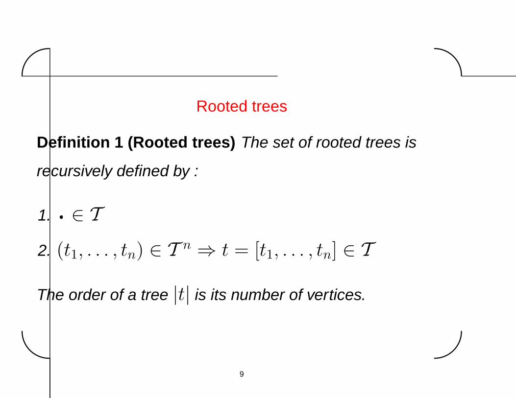
Rooted trees

Definition 1 (Rooted trees) The set of rooted trees is

recursively defined by :

1. ∈ T

2. (t1, . . . , tn) ∈ T n ⇒ t = [t1, . . . , tn] ∈ T

The order of a tree |t| is its number of vertices.

9

�

�

�

�

Examples of rooted trees

Arbre t

Ordre |t| 1 2 3 3 4 4 4 4

Symétrie σ(t) 1 1 2 1 6 1 2 1

TAB. 1 – Rooted trees of orders 1 to 4

10

�

�

�

�

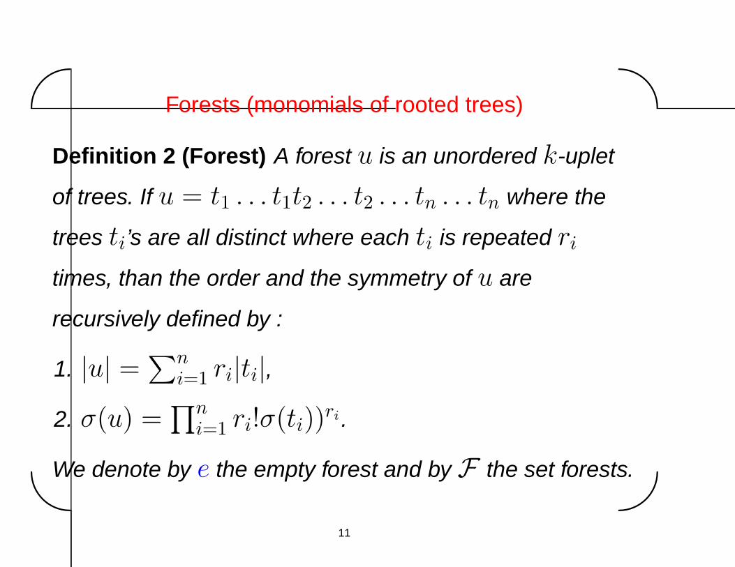
Forests (monomials of rooted trees)

Definition 2 (Forest) A forest u is an unordered k-uplet

of trees. If u = t1 . . . t1t2 . . . t2 . . . tn . . . tn where the

trees ti’s are all distinct where each ti is repeated ri

times, than the order and the symmetry of u are

recursively defined by :

1. |u| =∑n

i=1 ri|ti|,

2. σ(u) =∏n

i=1 ri!σ(ti))ri .

We denote by e the empty forest and by F the set forests.

11

�

�

�

�

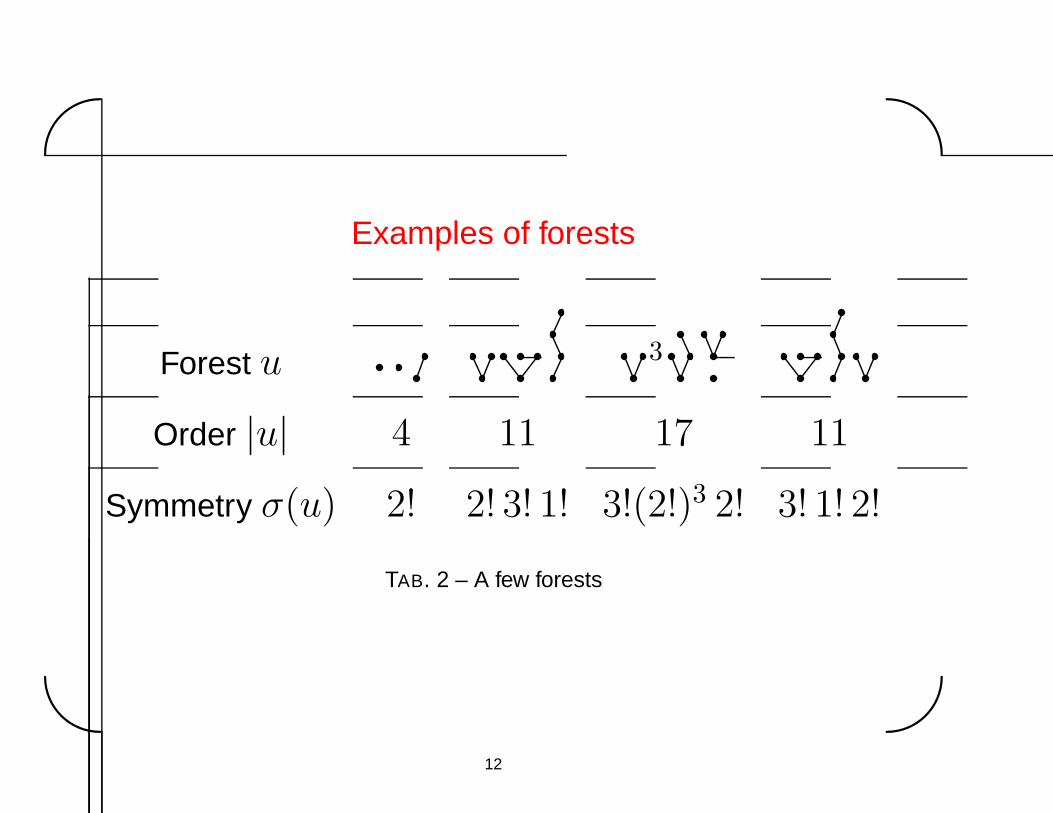
Examples of forests

Forest u 3

Order |u| 4 11 17 11

Symmetry σ(u) 2! 2! 3! 1! 3!(2!)3 2! 3! 1! 2!

TAB. 2 – A few forests

12

�

�

�

�

The algebra of forests

The set F can be naturally endowed with an algebra structure H on R :

– ∀ (u, v) ∈ F2, ∀ (λ, µ) ∈ R2, λu + µv ∈ H,

– ∀ (u, v) ∈ F2, u v ∈ H, where u v denotes the commutative product of the

forests u and v,

– ∀u ∈ F , u e = e u = u, where e is the empty forest.

Example of calculus in H :

(2 + 3 )( − + 8 ) = 2 − 2 + 16

+ 3 − 3 + 24

13

�

�

�

�

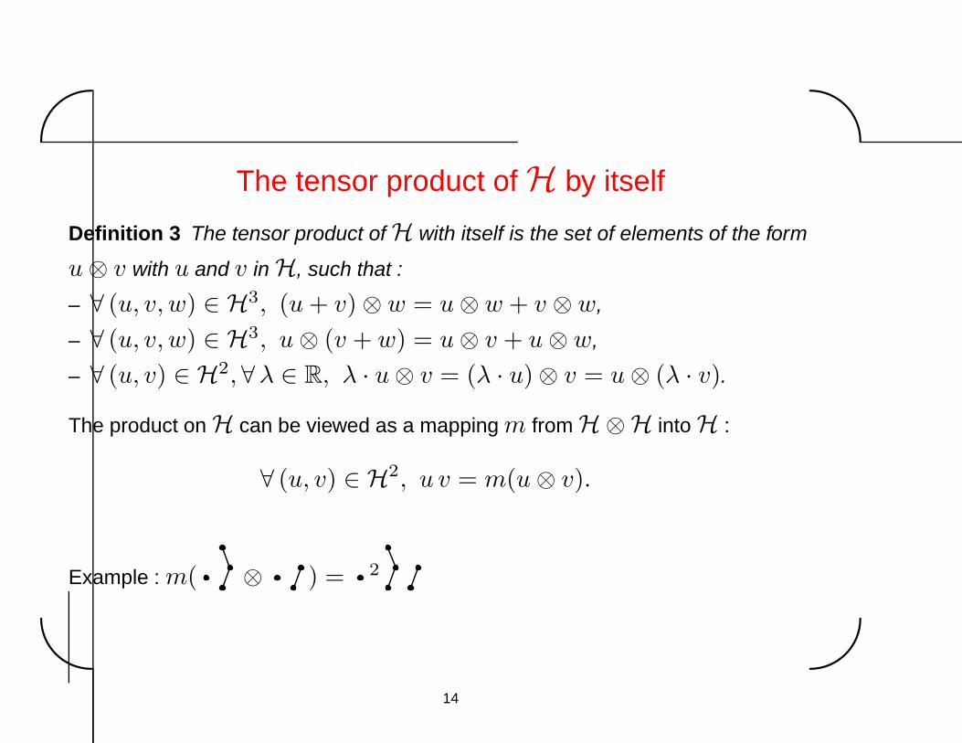
The tensor product of H by itself

Definition 3 The tensor product of H with itself is the set of elements of the form

u ⊗ v with u and v in H, such that :

– ∀ (u, v, w) ∈ H3, (u + v) ⊗ w = u ⊗ w + v ⊗ w,

– ∀ (u, v, w) ∈ H3, u ⊗ (v + w) = u ⊗ v + u ⊗ w,

– ∀ (u, v) ∈ H2, ∀λ ∈ R, λ · u ⊗ v = (λ · u) ⊗ v = u ⊗ (λ · v).

The product on H can be viewed as a mapping m from H⊗H into H :

∀ (u, v) ∈ H2, u v = m(u ⊗ v).

Example : m( ⊗ ) = 2

14

�

�

�

�

The co-product

We define the operators B+ and B− by :

B+ : H → Tu = t1 . . . tn → [t1, . . . , tn]

B− : T → Ht = [t1, . . . , tn] → t1 . . . tn

Examples : B+( ) =[ ]

= et B−( ) =

Definition 4 (Co-product) The co-product ∆ is a morphism from H to H⊗Hdefined recursively by :

1. ∆(e) = e ⊗ e,

2. ∀ t ∈ T , ∆(t) = t ⊗ e + (idH ⊗ B+) ◦ ∆ ◦ B−(t),

3. ∀u = t1 . . . tn ∈ F , ∆(u) = ∆(t1) . . .∆(tn).

15

�

�

�

�

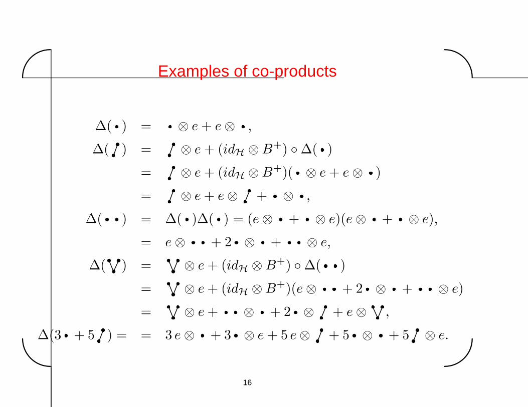
Examples of co-products

∆( ) = ⊗ e + e ⊗ ,

∆( ) = ⊗ e + (idH ⊗ B+) ◦ ∆( )

= ⊗ e + (idH ⊗ B+)( ⊗ e + e ⊗ )

= ⊗ e + e ⊗ + ⊗ ,

∆( ) = ∆( )∆( ) = (e ⊗ + ⊗ e)(e ⊗ + ⊗ e),

= e ⊗ + 2 ⊗ + ⊗ e,

∆( ) = ⊗ e + (idH ⊗ B+) ◦ ∆( )

= ⊗ e + (idH ⊗ B+)(e ⊗ + 2 ⊗ + ⊗ e)

= ⊗ e + ⊗ + 2 ⊗ + e ⊗ ,

∆(3 + 5 ) = = 3 e ⊗ + 3 ⊗ e + 5 e ⊗ + 5 ⊗ + 5 ⊗ e.

16

�

�

�

�

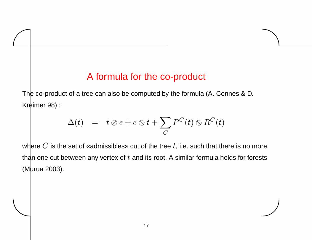
A formula for the co-product

The co-product of a tree can also be computed by the formula (A. Connes & D.

Kreimer 98) :

∆(t) = t ⊗ e + e ⊗ t +∑C

P C(t) ⊗ RC(t)

where C is the set of «admissibles» cut of the tree t, i.e. such that there is no more

than one cut between any vertex of t and its root. A similar formula holds for forests

(Murua 2003).

17

�

�

�

�

Elementary differentials

Definition 5 For each t ∈ T , the elementary differential F (t) associated with t is

the mapping from Rn to R

n, defined recursively by :

1. F ( )(y) = f(y),

2. F ([t1, . . . , tn])(y) = f (n)(y)(F (t1)(y), . . . , F (tn)(y)

).

Examples :

F ( )(y) = f ′(y)f(y),

F ( )(y) = f ′(y)f ′(y)f(y),

F ( )(y) = f (3)(y)(f(y), f(y), f(y)

).

18

�

�

�

�

B-series

Definition 6 (B-Series) Let a be a mapping from T to R. We define B(a, y), the

B-series associated with a, as the formal series :

B(a, y) = y +∑t∈T

h|t|

σ(t)a(t)F (t) = y + ha( )f(y) + h2a( )(f ′f)(y) + . . .

The exact solution of y = f(y) has a B-series expansion

B(1/γ, y) = y +∑t∈T

h|t|

γ(t)σ(t)F (t)(y)

= y + hf(y) +h2

2.1(f ′f)(y)

+h3

3.2(f ′′(f, f))(y) +

h3

6.1(f ′f ′f))(y) + . . .

19

�

�

�

�

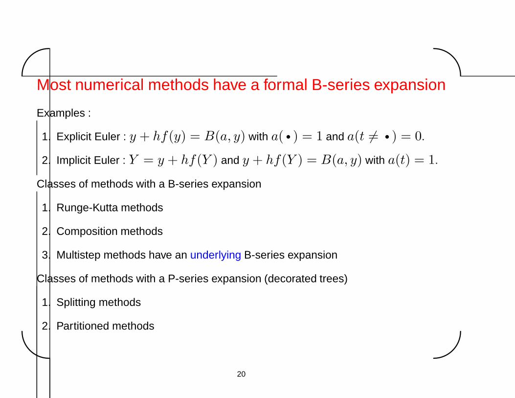
Most numerical methods have a formal B-series expansion

Examples :

1. Explicit Euler : y + hf(y) = B(a, y) with a( ) = 1 and a(t �= ) = 0.

2. Implicit Euler : Y = y + hf(Y ) and y + hf(Y ) = B(a, y) with a(t) = 1.

Classes of methods with a B-series expansion

1. Runge-Kutta methods

2. Composition methods

3. Multistep methods have an underlying B-series expansion

Classes of methods with a P-series expansion (decorated trees)

1. Splitting methods

2. Partitioned methods

20

�

�

�

�

Elementary differential operators

Definition 7 Let u = t1 . . . tk be a forest of F . The differential operator X(u)associated with u is defined on D = C∞(Rn; Rm) by :

X(u) : D → Dg → X(u)[g] = g(k)(F (t1), . . . , F (tk))

Examples :

X(e)[g] = g,

X( )[g] = g′f,

X( )[g] = g′f ′f,

X( )[g] = g(3)(f ′f, f, f

).

21

�

�

�

�

S-series

Definition 8 (Series of differential operators) Let α be a mapping from F into R.

We define S(α), the series of differential operators associated with α, as the formal

series

S(α)[g] =∑

u∈Fh|u|σ(u)α(u)X(u)[g]

For all g ∈ C∞(Rn; Rm) :

S(α)[g] = α(e)g + hα( )g′f +h2

2α( )g′′(f, f) + h2α( )g′f ′f + . . .

22

�

�

�

�

Composition of B-series and co-product in HTheorem 1 (Composition of B-series) Let a and b be two mappings from T to R.

The composition of the two B-series B(a, y) and B(b, y), i.e.

B(a, B(b, y))

is again a B-series, with coefficients ab defined on T by the composition law :

∀ t ∈ T , (ab)(t) = (a ⊗ b)∆(t).

Example :

(ab)( ) = (a ⊗ b)∆( )

= (a ⊗ b)(

⊗ e + (idH ⊗ B+) ◦ ∆( ))

= a( )b(e) + a( )a( )b( ) + 2a( )b( ) + a(e)b( )

23

�

�

�

�

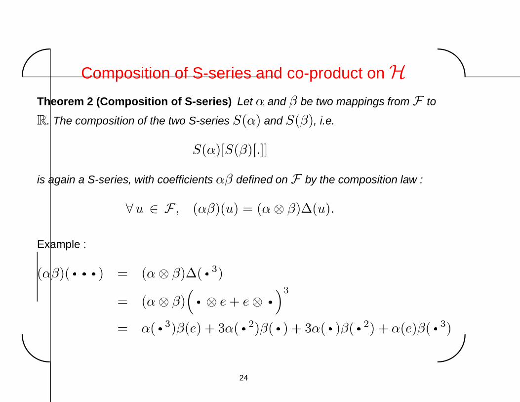
Composition of S-series and co-product on HTheorem 2 (Composition of S-series) Let α and β be two mappings from F to

R. The composition of the two S-series S(α) and S(β), i.e.

S(α)[S(β)[.]]

is again a S-series, with coefficients αβ defined on F by the composition law :

∀u ∈ F , (αβ)(u) = (α ⊗ β)∆(u).

Example :

(αβ)( ) = (α ⊗ β)∆( 3)

= (α ⊗ β)(

⊗ e + e ⊗)3

= α( 3)β(e) + 3α( 2)β( ) + 3α( )β( 2) + α(e)β( 3)

24

�

�

�

�

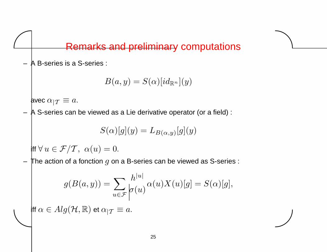
Remarks and preliminary computations

– A B-series is a S-series :

B(a, y) = S(α)[idRn ](y)

avec α|T ≡ a.

– A S-series can be viewed as a Lie derivative operator (or a field) :

S(α)[g](y) = LB(α,y)[g](y)

iff ∀u ∈ F/T , α(u) = 0.

– The action of a fonction g on a B-series can be viewed as S-series :

g(B(a, y)) =∑u∈F

h|u|

σ(u)α(u)X(u)[g] = S(α)[g],

iff α ∈ Alg(H, R) et α|T ≡ a.

25

�

�

�

�

Numerical methods preserving invariants

Let I be a first integral of y = f(y), i.e.

∀ y ∈ Rn,

(∇I(y)

)T

f(y) = 0.

The numerical method associated with the B-series B(a, y) preserves I iff

∀ y ∈ Rn, I

(B(a, y)

)= I(y),

i.e.

S(α)[I] = I,

where α is the unique algebra-morphism extending a onto H.

26

�

�

�

�

The annihilating left ideal I[I] of I (part I)

In algebraic terms, saying that I is an invariant can be written

X( )[I] = 0.

If S(ω) acts on X( )[I] from the left, one gets :

S(ω)[hX( )[I]] = S(ω′)[I] = 0,

with

∀u = t1 . . . tm ∈ F , ω′(u) =m∑

i=1

ω(B−(ti)

∏j �=i

tj

).

Example :

ω′( ) = ω( ) + ω( ) + ω( )

27

�

�

�

�

The annihilating left ideal I[I] of I (part II)

Lemma 1 Consider δ ∈ H∗. Then, δ ∈ I[I] if and only if δ(e) = 0 and for all

trees t1, . . . , tm de T , one has :

δ(t1 . . . tm) =m∑

j=1

δ(tj ◦

∏i �=j

ti

).

Notation :

s ◦ (t1t2 . . . tm) = B+(B−(s)t1t2 . . . tm

).

Examples :

– Pour m = 2 : δ( ) = δ( ) + δ( ).

– Pour m = 3 : δ( ) = 2δ( ) + δ( )

28

�

�

�

�

Integrators preserving general invariants

Theorem 3 Let α ∈ Alg(H, R). Then α satifies S(α)[I] = I that for all couples

(f, I) of a vector field f and a first integral I , if and only if α(e) = 1 and α

satisfies the condition

α(t1) · · ·α(tm) =∑m

j=1 α(tj ◦∏

i �=j ti)

for all m ≥ 2 and all ti’s in T .

Theorem 4 A B-series integrator that preserves all cubic polynomial invariants does

in fact preserve polynomial invariants of any degree, and thus is the B-series

corresponding to the (scaled) exact flow.

Consequence : There remains hope only for quadratic invariants.

29

�

�

�

�

Integrators preserving quadratic invariants

Theorem 5 Let α ∈ Alg(H, R). Then α satifies S(α)[I] = I that for all couples

(f, I) of a vector field f and a quadratic first integral I , if and only if α(e) = 1 and

α satisfies the condition

α(t1)α(t2) = α(t1 ◦ t2) + α(t2 ◦ t1)

for all pairs (t1, t2) ∈ T 2.

Example : A B-series integrator B(a, y) preserve quadratic invariants (m = 2) if

and only if, for all pairs of trees (t1, t2) ∈ T 2, the following relation holds :

a(t1 ◦ t2) + a(t2 ◦ t1) = a(t1)a(t2).

This condition is also the condition for B(a, y) to be symplectic.

30

�

�

�

�

Integrators preserving Hamiltonian invariants

We now turn our attention to systems of the form y = f(y) with

f(y) = J−1∇H(y),

and we explore the conditions under which a B-series integrator B(a, y) preserves

exactly the Hamiltonian function, i.e.

S(α)[H] = H

where α is the only algebra morphism such that α|T ≡ a.

31

�

�

�

�

Elementary Hamiltonians

We define the elementary Hamiltonian H(t) as the mapping from Rn to R

obtained recursively by :

H( )(y) = H(y),

H([s1, . . . , sn, t]) = H(n+1)(F (s1), . . . , F (sn), F (t)

),

=(F (t)

)T

J(J−1∇H

)(n)(F (s1), . . . , F (sn)

)

=(F (t)

)T

JF (s) = H(s ◦ t)

Lemma 2 Let s and t be two trees of T . We have the relation :

H(s ◦ t) = −H(t ◦ s).

32

�

�

�

�

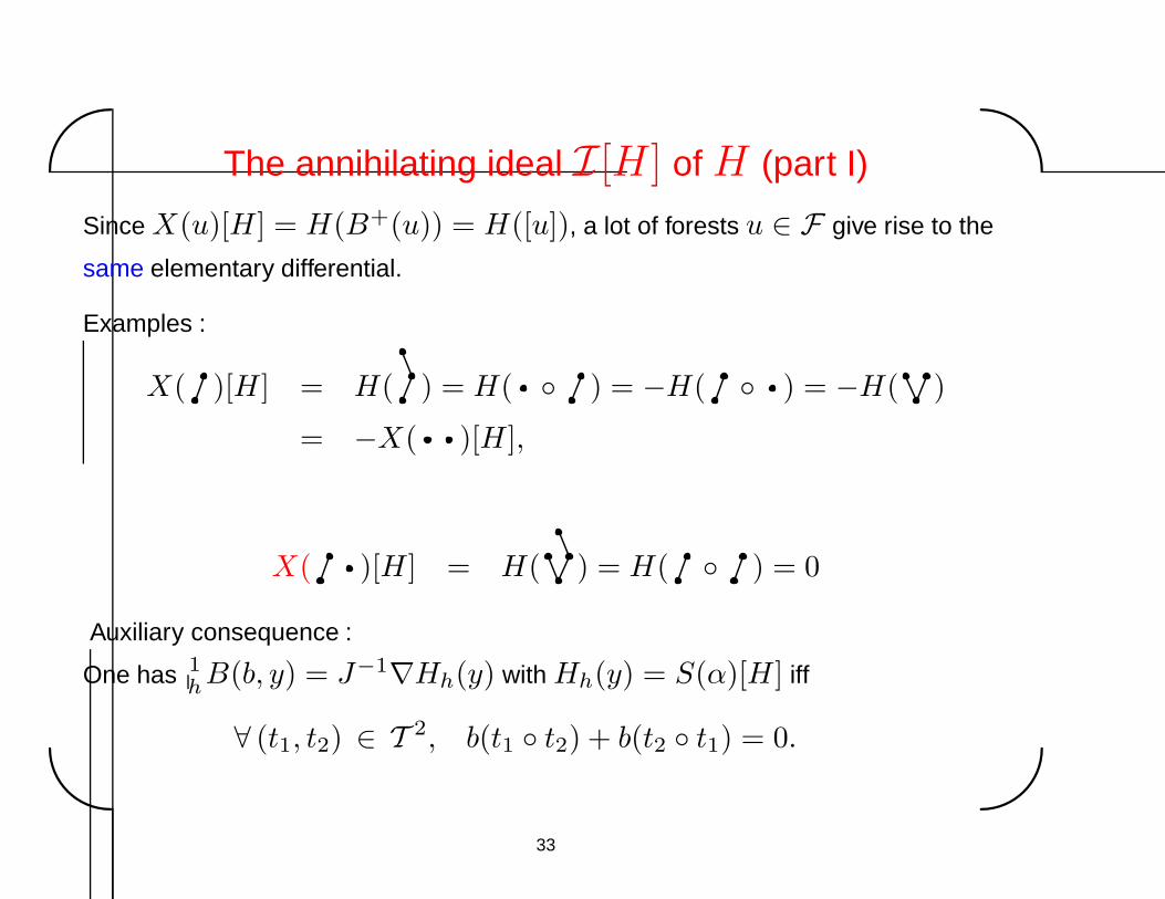
The annihilating ideal I[H] of H (part I)

Since X(u)[H] = H(B+(u)) = H([u]), a lot of forests u ∈ F give rise to the

same elementary differential.

Examples :

X( )[H] = H( ) = H( ◦ ) = −H( ◦ ) = −H( )

= −X( )[H],

X( )[H] = H( ) = H( ◦ ) = 0

Auxiliary consequence :

One has 1hB(b, y) = J−1∇Hh(y) with Hh(y) = S(α)[H] iff

∀ (t1, t2) ∈ T 2, b(t1 ◦ t2) + b(t2 ◦ t1) = 0.

33

�

�

�

�

The set HS of non-superfluous free trees

We define an equivalence class t as being the set of trees that can be obtained from

t by changing the position of the root.

Examples : For t = , t = { , }. For t = , t = { , }.

Given a total order ≥ on T , compatible with | · |, the set HS is defined by

t ∈ HS iff t = or ∃ (s1, s2) ∈ T 2, s1 > s2, t = s1 ◦ s2.

The set HS is the set of representatives of equivalence classes whose elementary

differential does not vanish. The first of these are :

/∈ HS , /∈ HS , ∈ HS , /∈ HS , /∈ HS , ∈ HS , /∈ HS .

34

�

�

�

�

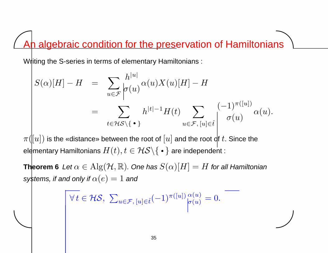
An algebraic condition for the preservation of Hamiltonians

Writing the S-series in terms of elementary Hamiltonians :

S(α)[H] − H =∑u∈F

h|u|

σ(u)α(u)X(u)[H] − H

=∑

t∈HS\{ }

h|t|−1H(t)∑

u∈F , [u]∈t

(−1)π([u])

σ(u)α(u).

π([u]) is the «distance» between the root of [u] and the root of t. Since the

elementary Hamiltonians H(t), t ∈ HS\{ } are independent :

Theorem 6 Let α ∈ Alg(H, R). One has S(α)[H] = H for all Hamiltonian

systems, if and only if α(e) = 1 and

∀ t ∈ HS,∑

u∈F , [u]∈t(−1)π([u]) α(u)σ(u) = 0.

35

�

�

�

�

Example : the fifth-order condition for tII =

tII ={

, [ ], [ , ], [ ]}

B− ↓ B− ↓ B− ↓ B− ↓

(−1)π/σ ↓ (−1)π/σ ↓ (−1)π/σ ↓ (−1)π/σ ↓

13! − 1

2! − 13!

13!

α ↓ α ↓ α ↓ α ↓

0 = 13!α( )3α( ) − 1

2!α( ) − 13!α( )α( ) + 1

3!α( )

36

�

�

�

�

The non-existence of symplectic Hamiltonian preserving

integrators

Theorem 7 Suppose a B-series integrator B(α, y) satisfies both conditions

∀ (t1, t2) ∈ T 2, α(t1)α(t2) = α(t1 ◦ t2) + α(t2 ◦ t1)

∀ t ∈ HS,∑

u∈F , [u]∈t

(−1)π([u]) α(u)σ(u)

= 0.

for the preservation of quadratic invariants and for the preservation of exact

Hamiltonians. Then it is the B-series of the scaled exact flow.

There exists no symplectic numerical method that preserves the Hamiltonian exactly

37

�

�

�

�

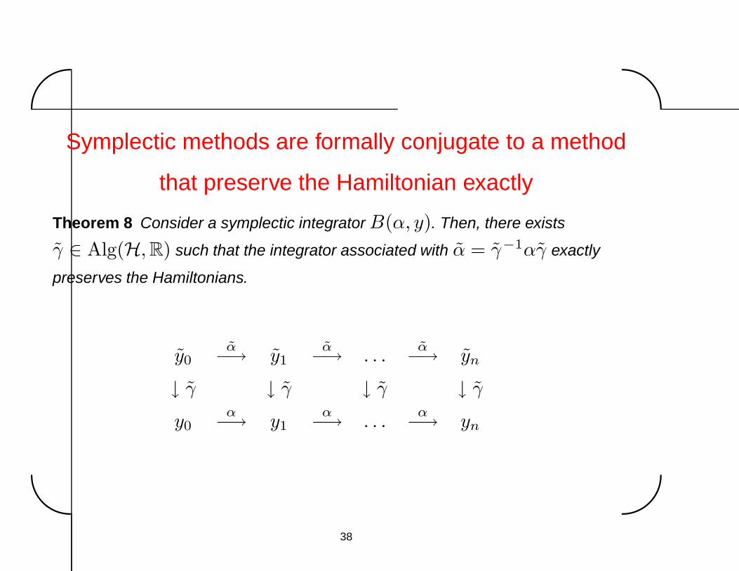
Symplectic methods are formally conjugate to a method

that preserve the Hamiltonian exactly

Theorem 8 Consider a symplectic integrator B(α, y). Then, there exists

γ ∈ Alg(H, R) such that the integrator associated with α = γ−1αγ exactly

preserves the Hamiltonians.

y0α−→ y1

α−→ . . .α−→ yn

↓ γ ↓ γ ↓ γ ↓ γ

y0α−→ y1

α−→ . . .α−→ yn

38

�

�

�

�

PART II : modified equations

39

�

�

�

�

Backward error analysis

The fundamental idea of backward error analysis consists in interpreting the

numerical solution y1 = Φfh(y0)

y = f(y),

y(0) = y0,

as the exact solution of a modified differential equation

˙y = f(y),

y(0) = y0.

40

�

�

�

�

Partitions and skeletons

Definition 9 (Partitions of a tree) The partition pτ of a tree τ ∈ T is the tree

obtained from τ by replacing some of its edges by dashed ones. We denote

P (pτ ) = {s1, . . . , sk} the list of subtrees si ∈ T obtained from pτ by removing

dashed edges. The set of all partitions pτ of τ is denoted P(τ).

Definition 10 The skeleton χ(pτ ) ∈ T of a partition pτ ∈ P(τ) of a tree τ ∈ Tis the tree obtained by replacing in pτ each tree of P (pτ ) by a single vertex and

then dashed edges by solid ones. We can notice that |χ(pτ )| = #pτ .

41

�

�

�

�

Example : The 8 partitions of tree τ = [[•, •]] with

corresponding skeletons and lists

pτ ∈ P(τ)

#pτ 1 2 2 2 3 3 3 4

χ(pτ )

P (pτ ) , , , 2, 2, 2, 4

42

�

�

�

�

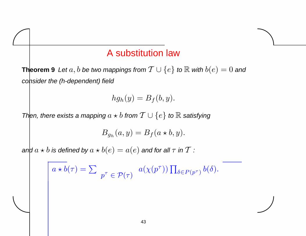
A substitution law

Theorem 9 Let a, b be two mappings from T ∪ {e} to R with b(e) = 0 and

consider the (h-dependent) field

hgh(y) = Bf (b, y).

Then, there exists a mapping a � b from T ∪ {e} to R satisfying

Bgh(a, y) = Bf (a � b, y).

and a � b is defined by a � b(e) = a(e) and for all τ in T :

a � b(τ) =∑

pτ ∈ P(τ)a(χ(pτ ))

∏δ∈P (pτ ) b(δ).

43

�

�

�

�

A few terms of the substitution law

a � b( ) = a( )b( ),

a � b( ) = a( )b( ) + a( )b( )2,

a � b( ) = a( )b( ) + 2a( )b( )b( ) + a( )b( )3,

a � b( ) = a( )b( ) + a( )b( )b( ) + 2a( )b( )b( )

+a( )b( )2b( ) + 2a( )b( )2b( ) + a( )b( )4,

a � b( ) = a( )b( ) + 2a( )b( )b( ) + a( )b( )2

+3a( )b( )2b( ) + a( )b( )4.

44

�

�

�

�

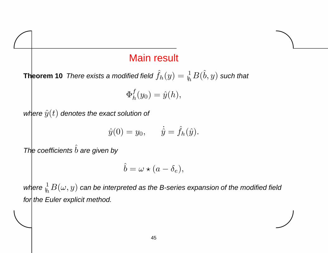
Main result

Theorem 10 There exists a modified field fh(y) = 1hB(b, y) such that

Φfh(y0) = y(h),

where y(t) denotes the exact solution of

y(0) = y0, ˙y = fh(y).

The coefficients b are given by

b = ω � (a − δe),

where 1hB(ω, y) can be interpreted as the B-series expansion of the modified field

for the Euler explicit method.

45

�

�

�

�

Main consequence

Theorem 11 Consider a B-series with coefficients a satisfying the condition :

∀m, 2 ≤ m ≤ n, ∀(u1, . . . , um) ∈ T m,m∑

i=1

a(ui ◦∏j �=i

uj) =m∏

i=1

a(ui).

Then the coefficients b of its modified equation satisfy :

∀m, 2 ≤ m ≤ n, ∀(u1, . . . , um) ∈ T m,m∑

i=1

b(ui ◦∏j �=i

uj) = 0.

The converse is also true.

46