Embed Size (px)
Citation preview

Introduction to SPSS – A Tutorial for SPSS v20
As with any software package, there are multiple ways to perform any task. In order to
avoid confusion for the beginning user, in most cases only one method of performing a
task is explained. This does not mean that this is the only way to perform the task; just
that it is the easiest way to either explain or learn.
Accessing the SPSS Software
The University of Auckland has a site licence for SPSS Statistics. This means that you will
be able to use the software anywhere on campus. If SPSS is not installed on your UoA
office/laboratory computer, please contact your departmental IT support team to discuss
access. University of Auckland staff and postgraduate students are eligible to install SPSS
on one personal computer for work at home purposes. An installation DVD is available for
purchase from the IC Helpdesk, Level 2, Kate Edger Information Commons, City Campus.
A small cost will apply for the CD. Staff and postgrad students are required to produce
their staff / student ID and sign the SPSS Use Terms form prior to receiving the media kit.
Undergraduate students wishing to install SPSS on their home computer can purchase a
licence for the IBM SPSS Statistics Standard Grad Pack v20 at
www.studentdiscounts.com.au. You must be a currently enrolled student (proof is
required) and intend to use the product for educational purposes only. Installation on a
network or in an academic lab is strictly prohibited by the license agreement. The student
version expires after 13 months.
Getting Further Assistance
Postgraduate students who require further assistance with SPSS software in order to
analyze own data sets, can contact the Student Learning Centre (SL) reception and ask
for a one-to-one tutoring appointment with a respective tutor, however, our role is merely
advisory. Please do not ask us to analyze your data for you, as refusal may offend.
For further information about basic facts and FAQs on SPSS go to:
http://cad.auckland.ac.nz/index.php?p=data_analysis. This link also takes you to our
examples and the survey data set we are using in this workshop.
For advanced courses using SPSS you may like to attend the workshops SPSS
Intermediate for Postgraduates I: Comparing Means and/or SPSS Intermediate for
Postgraduates II:Correlations and Related Procedures which cover statistical theory with
hands on experience in relation to SPSS.
Finally, please keep in mind that it is your supervisor’s responsibility to advise you on your
statistical analysis approach.
Student Learning Services (Tā te Ākonga)

Student Learning Services©2013; M. Blumenstein (Senior Tutor-Data Analysis)
2
Opening the SPSS Program
SPSS is likely to be located on the Programs menu from the Start button. When SPSS
opens, the following dialog box appears:
Once this occurs, click on the Cancel button. You should now be in the SPSS Statistics
Data Editor - this will resemble a spreadsheet and is where you will enter, edit, and
display, the contents of your data file.
Opening a File in SPSS
The data that will be used for today’s tutorial is based on a questionnaire. During the
workshop all sample files are available from your local computer under SLC
ShareStudent FilesIn Class Files spss_tut_file.
If you like to practice further after completion of this workshop you may
want to access a copy of this file or other examples from the SLC website
at another time:
http://www.cad.auckland.ac.nz/content/files/slc/computer_spss_tut_file.sav
To open a new file, from the SPSS menu bar, select:

Student Learning Services©2013; M. Blumenstein (Senior Tutor-Data Analysis)
3
To open a blank file for entering a new data set from the menu bar select
File NewData
or click on the open file icon of the SPSS data editor menu bar:
What can we see in this data set?
Once the 'spss_tut_file' file is open, we will see the following screen in the Variable View:
Variable View
Variable and Data View
In SPSS there are two different 'views', the Data View and the Variable View.
You can alternate between these two views by clicking on their
tabs at the bottom left-hand side of your screen.
Student Learning Services©2013; M. Blumenstein (Senior Tutor-Data Analysis)
4
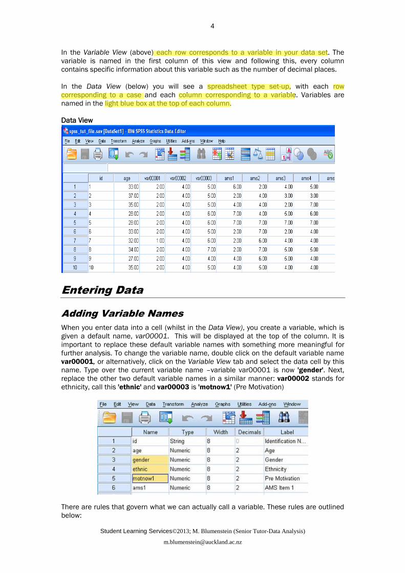
In the Variable View (above) each row corresponds to a variable in your data set. The
variable is named in the first column of this view and following this, every column
contains specific information about this variable such as the number of decimal places.
In the Data View (below) you will see a spreadsheet type set-up, with each row
corresponding to a case and each column corresponding to a variable. Variables are
named in the light blue box at the top of each column.
Data View
Entering Data
Adding Variable Names
When you enter data into a cell (whilst in the Data View), you create a variable, which is
given a default name, var00001. This will be displayed at the top of the column. It is
important to replace these default variable names with something more meaningful for
further analysis. To change the variable name, double click on the default variable name
var00001, or alternatively, click on the Variable View tab and select the data cell by this
name. Type over the current variable name –variable var00001 is now 'gender'. Next,
replace the other two default variable names in a similar manner: var00002 stands for
ethnicity, call this 'ethnic' and var00003 is 'motnow1' (Pre Motivation)
There are rules that govern what we can actually call a variable. These rules are outlined
below:

Student Learning Services©2013; M. Blumenstein (Senior Tutor-Data Analysis)
5
Each variable name must be unique; duplication is not allowed.
Variable names can be up to 64 bytes long, and the first character must be a letter
or one of the characters @, #, or $. Subsequent characters can be any
combination of letters, numbers, non-punctuation characters, and a period (.). In
code page mode, sixty-four bytes typically means 64 characters in single-byte
languages (for example, English, French, German, Spanish, Italian, Hebrew,
Russian, Greek, Arabic, and Thai) and 32 characters in double-byte languages (for
example, Japanese, Chinese, and Korean).
Reserved keywords cannot be used as variable names. Reserved keywords are
ALL, AND, BY, EQ, GE, GT, LE, LT, NE, NOT, OR, TO, and WITH.
The period, the underscore, and the characters $, #, and @ can be used within
variable names. For example, A._$@#1 is a valid variable name.
Variable names cannot contain spaces
Often variable names are truncated or abbreviated and Variable Labels are assigned
which give a more detailed description of the variable or a more meaningful name.
Assigning Variable Labels
While still in the Variable View, click in the Label column in the row that matches the
'gender' variable. Gender is pretty self-explanatory so we don’t really need to lengthen this
but we may want to capitalise this, as we couldn’t do so earlier. Type Gender in the
selected cell, and then type Ethnicity in the 'ethnic' row.In the ‘motnow1’ row, we want to
put something t more meaningful so type Pre Motivation in the cell matching the row and
column for this variable. This corresponds to the participant’s motivation before
completing the questionnaire.
In Data View, if you hold your mouse over the short variable names in the blue
boxes at the top of each column, the full variable name will appear.
Assigning Value Labels
Our data with respect to gender and ethnicity are actually made up of numbers that
correspond to 'groupings' or categorical data. For example, for the ‘Gender’ variable we
have males and females in our study. In SPSS we assign 1=male and 2=female.

Student Learning Services©2013; M. Blumenstein (Senior Tutor-Data Analysis)
6
It is also possible to enter actual words i.e. ‘string’ variables into SPSS, but
if we entered ‘Male’ and ‘Female’ in this way we would not be able to use
them in statistical analyses. If you do wish to enter words as part of your
data set however, in the Variable View, in the ‘Type’ column for your
variable, click on the blue box (with the three dots) that appears, and
change to ‘String’ then click ‘OK’ button.
Whilst still in the Variable View, click on the row for Gender and the column that is
headed Values. Click on the blue box with the three dots and this will open the Value
Labels dialog box.
Type 1 in the Value text box and Male in the Value Label text
box. Click on Add.
Type 2 in the Value text box. Type Female in the Value Label
text box. Click on Add. Click on OK.
Now assign value labels for the ethnicity variable using a similar procedure. The value
labels for this variable are as follows:
1=Pakeha
2=NZ Maori
3=Pacific Island
4=Asian
5=Other
In data view, display the value labels for gender and ethnicity by clicking on
to switch between numbers or labels in our data set. Any output will show the labels as
opposed to the somewhat meaningless numbers.
Entering Data
Data are entered into SPSS in the Data View mode. For example start with the ID number
of a single participant in the selected cell then move within that row to the next cell by
pressing the right arrow key i.e. enter the data for age, gender, ethnicity etc in this
manner. When you come to enter variables that we assigned ‘value labels’ for (eg gender,

Student Learning Services©2013; M. Blumenstein (Senior Tutor-Data Analysis)
7
ethnicity), you can choose the appropriate label from a drop-down list if you have SPSS
set to show the labels as opposed to the numbers.
Saving Your Data Files
Use the ‘Save As’ command from the file menu and then save the amended version of
your spss_tut_file under an alternative name (eg ‘motivation data) on the desktop.
Choose ‘Save’ from the file menu to save the most recent version of your file, and ‘Save
As’ if you wish to save an alternative version. It is wise to save your data periodically in
case your computer crashes. Always remember to keep back-up copies!
Other Points Regarding Data Entry
Missing Values
It is unlikely that you will receive a full set of data for all your cases. Inevitably, people
accidentally miss questions, refuse to answer them, or generally don’t read instructions.
This means not every cell in every row and every column has something in them. It is
possible to just leave these cells empty; SPSS treats these missing values as system-
missing. SPSS will exclude system-missing values from its calculations of means,
standard deviations and other statistics.
However, you can also assign missing value codes if you wish to know why a value is
missing. For example, suppose in an exam, some students either walked out as soon as
they saw the paper or, having at least attempted to answer some questions but have
earned only a very low mark (say 20% or less). You might wish to treat these occurrences
(user-missing values) in the following way so that you have an idea about the relative
frequencies in your data output later on (missing value analysis):
1. Any marks between 0-20
2. Cases who did not attempt to answer any exam questions (walk-out)
To assign missing value codes, whilst in Variable View select the appropriate ‘Missing’
cell for the row matching the appropriate variable. Once the appropriate cell is selected,
click on the small grey box with the three dots (…) that appears. This will bring up a dialog
box that allows you to assign missing values.
A walk-out could be coded as an arbitrary number such as ‘-9’; the negative sign helps to
stand out as an impossible real value. For a Likert Type Scale from 1-7 one could use a
‘9’ for a missing value. However if you are expecting data between 5 to 65 for the age of
a participant in your study, ‘9’ would not be suitable as a user-missing value and a ‘99’ or

Student Learning Services©2013; M. Blumenstein (Senior Tutor-Data Analysis)
8
‘999’ is more appropriate as it is outside any naturally occurring value specific to your
data set.
Select the appropriate option by clicking on its radio button (see above) and enter the
missing value(s) you have decided on (note that you don’t need to enter in more than
one). Click on OK to return to the Variable View. All empty cells with respect to exam mark
will now be replaced with a ‘-9’ in your data set.
Other Properties of Variables
In the ‘Variable View’ we can also set a number of other ‘properties’ such as the number
of decimal places shown, the variable type, and measurement level (data type i.e.
nominal, ordinal or scalar).
Inserting and Deleting Variables and Cases
To insert a new case between existing cases in “Data View” select a cell in the case (row)
below where you wish the new case to appear, and choose: EditInsert Case
To insert a new variable between existing variables select a cell in the variable (column)
to the right of where you wish the new variable to appear, choose EditInsert Variable
To delete a case or variable in Data View select the case number on the far left side of
the row(s) or the variable name at the top of the column(s) you wish to delete, and from
the menu bar choose: EditClear
Creating a New SPSS File
In the following drug experiment example where we look at performance (score) and
under three different treatments (group) we are creating a new SPSS file using the data
presented in the table below. From the menu bar in the Data Editor choose:
FileNew (data)
In Variable View define your variables first, then in Data View enter your values row by row
accordingly using the data set below.
Ensure that you name and label your variables appropriately.
Assign value labels for ‘Gender’ (1=male and 2=female) and ‘Group’(1=Placebo,
2=Drug A, 3=Drug B).
For unknown ‘Score’, assign ‘99’ as a missing value.
Case# Name Age Gender Group Score
1 Smith 38 Male Placebo 9.51
2 Taylor 28 Female Placebo 6.45
3 Myers 25 Female Drug A 8.88
4 Bungle 37 Male Drug B 5.92
Insert a new participant with the name of ‘Baldwin’ between case 3 and 4 using the
following details: Case# 5, 30 year old female treated with Drug B resulting in a
score of 5.87. Save your data file as ‘Drug Experiment’ on the desk top.
Finding and Correcting Errors in Data Entry
Mistakes occurring during data entry can have detrimental effects on your analysis
(outliers for example). A good way to find mistakes in your data is to run descriptive
statistics over them. For example, if your age groups are only meant to range from 15 to

Student Learning Services©2013; M. Blumenstein (Senior Tutor-Data Analysis)
9
25 and you have values below and higher than this, then you know you have made
mistakes that need to be fixed! Make sure you hunt out these errors before running any
final analyses. To correct a mistake, simply select the cell in which there is an error, and
type over it.
Data in Non-SPSS Formats
Excel, SAS and other file formats can be opened in SPSS directly (you may need to
change the ‘Files of Type’ box to ‘All Files’ before you can see your file to open it). If your
file is in another spreadsheet type package which is not supported by SPSS then you may
first need to save your file in ‘Tab Delimited’ format before attempting to open it in SPSS.
Upon opening, an import wizard guide you through the steps needed to open your tab-
delimited file. Note that when your file is opened in SPSS, any variable names that do not
conform to the naming rules will be altered. Also keep in mind that you can copy and
paste your data, but your variable names will not transfer across with your data if you do
so. Often some recoding needs to be done and value labels have to added in SPSS.
Working with Data
Compute a new variable using the calculator pad
SPSS has a 'Compute' function that allows us to calculate new variables very quickly. In
the data set we are presently using, we wish to add the individual items for Social
Responsibility together to give us a 'Total Social Responsibility' score. From the menu bar
choose: TransformCompute
The Compute Variable box will appear. Enter the target variable name. For the purposes
of this tutorial this name will be totsr.
Next click the Type & Label box underneath this name and enter the label Total Social
Responsibility followed by Continue.
From the variable list (the box on the far left of the Compute Variable box) select the
variable ‘sr1’ or ‘Social Resp Item 1’. Now add this variable into your numerical
expression by clicking on the small arrow to the right of the variable list. Next, click on ‘+’
on the calculator pad. This sign should also have appeared in your Numeric Expression
box. Keep adding the social responsibility items separated by the ‘+’ sign until all five are
added in this manner. Your dialog box should look as follows:

Student Learning Services©2013; M. Blumenstein (Senior Tutor-Data Analysis)
10
Compute a new variable using a function
To add up the motivation items into a 'Total Motivation Score', we will use the SUM
function. From the menu bar select: TransformCompute
The Compute Variable box will appear. Enter the target variable name totmot. To add a
label for this variable, click on the Type & Label button.
Enter the numerical expression for this target variable. From the list of functions in the
pane on the right hand side, select Sum from the statistical function group. Using the
upwards pointing arrow add Sum into your Numeric Expression box.
Replace the question marks by moving all twelve motivation items (ams1 to ams12) into
the brackets. Each item needs to be separated by a comma. Use the arrow pointing
towards the right to add the motivation items into the numeric expression box.
Alternatively, double click on the variable while the cursor is located in the bracket.
Click on OK and your target variable will appear in your data set (located at far right).
Recoding Variables
It is also possible for us to recode variables. We are going to recode our age data into
three groups for the purposes of a later analysis. The ages in this data set range from 21
years upwards (these students were postgraduates, hence the slightly older age bracket).
We want to split these ages into the following groups:
21 years to 28 years
29 years to 35 years
36 years onwards
From the menu bar, select: TransformRecodeInto Different Variables
Select the age variable and add it into the Input Variable -> Output Variable box. Next, in
the Output Variable Name box type agegrp and for the label type Age Group. Now click
on the Change button.
Student Learning Services©2013; M. Blumenstein (Senior Tutor-Data Analysis)
11
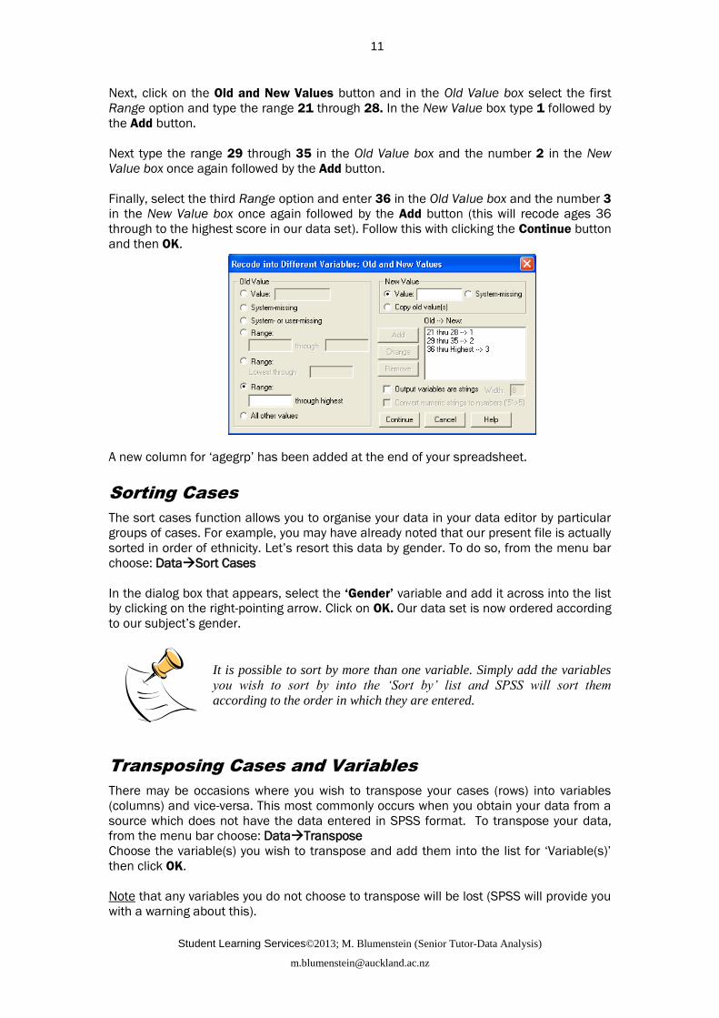
Next, click on the Old and New Values button and in the Old Value box select the first
Range option and type the range 21 through 28. In the New Value box type 1 followed by
the Add button.
Next type the range 29 through 35 in the Old Value box and the number 2 in the New
Value box once again followed by the Add button.
Finally, select the third Range option and enter 36 in the Old Value box and the number 3
in the New Value box once again followed by the Add button (this will recode ages 36
through to the highest score in our data set). Follow this with clicking the Continue button
and then OK.
A new column for ‘agegrp’ has been added at the end of your spreadsheet.
Sorting Cases
The sort cases function allows you to organise your data in your data editor by particular
groups of cases. For example, you may have already noted that our present file is actually
sorted in order of ethnicity. Let’s resort this data by gender. To do so, from the menu bar
choose: DataSort Cases
In the dialog box that appears, select the ‘Gender’ variable and add it across into the list
by clicking on the right-pointing arrow. Click on OK. Our data set is now ordered according
to our subject’s gender.
It is possible to sort by more than one variable. Simply add the variables
you wish to sort by into the ‘Sort by’ list and SPSS will sort them
according to the order in which they are entered.
Transposing Cases and Variables
There may be occasions where you wish to transpose your cases (rows) into variables
(columns) and vice-versa. This most commonly occurs when you obtain your data from a
source which does not have the data entered in SPSS format. To transpose your data,
from the menu bar choose: DataTranspose
Choose the variable(s) you wish to transpose and add them into the list for ‘Variable(s)’
then click OK.
Note that any variables you do not choose to transpose will be lost (SPSS will provide you
with a warning about this).
Student Learning Services©2013; M. Blumenstein (Senior Tutor-Data Analysis)
12
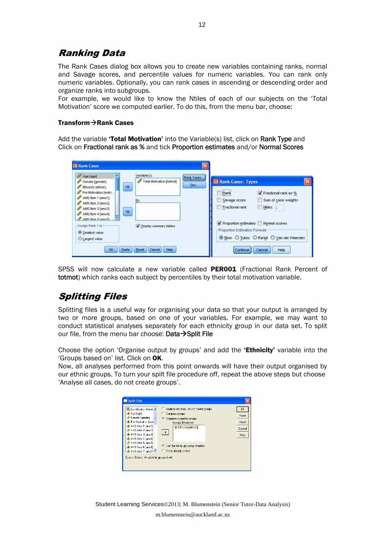
Ranking Data
The Rank Cases dialog box allows you to create new variables containing ranks, normal
and Savage scores, and percentile values for numeric variables. You can rank only
numeric variables. Optionally, you can rank cases in ascending or descending order and
organize ranks into subgroups.
For example, we would like to know the Ntiles of each of our subjects on the ‘Total
Motivation’ score we computed earlier. To do this, from the menu bar, choose:
TransformRank Cases
Add the variable ‘Total Motivation’ into the Variable(s) list, click on Rank Type and
Click on Fractional rank as % and tick Proportion estimates and/or Normal Scores
SPSS will now calculate a new variable called PER001 (Fractional Rank Percent of
totmot) which ranks each subject by percentiles by their total motivation variable.
Splitting Files
Splitting files is a useful way for organising your data so that your output is arranged by
two or more groups, based on one of your variables. For example, we may want to
conduct statistical analyses separately for each ethnicity group in our data set. To split
our file, from the menu bar choose: DataSplit File
Choose the option ‘Organise output by groups’ and add the ‘Ethnicity’ variable into the
‘Groups based on’ list. Click on OK.
Now, all analyses performed from this point onwards will have their output organised by
our ethnic groups. To turn your spilt file procedure off, repeat the above steps but choose
‘Analyse all cases, do not create groups’.
Student Learning Services©2013; M. Blumenstein (Senior Tutor-Data Analysis)
13
Selecting Cases
A similar procedure to splitting your file is that of selecting cases. It is possible to ask
SPSS to only perform analyses on a certain subset of your data, for example, only the
males or only students who scored above a certain point on your questionnaire.
To select a subset of cases, from the menu bar choose: DataSelect Cases
In the dialog box that appears, select If condition is satisfied and click on the If button
that appears underneath. Add the ‘Gender’ variable across using the right-pointing arrow.
Press the '=' button on the calculator pad and then type the number 1. Only male
subjects in our sample are now selected.
Select Continue followed by OK. In the Data Editor your data will now show ‘slashed lines’
through any subject that was not male. Any output that is created will be based only on
those selected subjects (in this case, males). To select all your cases once again, repeat
the above steps, this time choosing the ‘All Cases’ option.
Merging Files
There are two instances where you may wish to merge files. Firstly, you may have two
different sets of data which have the same variables but different cases – for instance,
two researchers may have collected the same set of data for two different populations
and then wish to combine them. Secondly, you may have collected data from the same
set of subjects (cases) but have two different sets of variables for these.
To merge files, ensure that your files are saved in SPSS format and that they are sorted in
order by the key field (eg. ID number). Open up your base file, select: DataMerge Files
Followed by the type of merge you require. Select the file you wish to be merged and then
follow the on screen instructions.
Student Learning Services©2013; M. Blumenstein (Senior Tutor-Data Analysis)
14
Calculating Simple Statistics
Frequencies
Say we wanted to know how many students in our sample were of each gender. To
calculate this we use the Frequency procedure. From the menu, choose:
AnalyzeDescriptive StatisticsFrequencies
This will open the Frequencies box. Select ‘Gender’ as a variable and click on the small
arrow to the right of the variable list. The variable ‘Gender’ should now have moved into
the box headed Variable(s). Click on OK.
The SPSS output viewer will appear displaying all the data from your stats procedures.
Information contained in your
Output Viewer needs to be SAVED
SEPARATELY from your data
files. These files are of a different
type and are given the file
extension ‘*.spv’ as opposed to the
‘*.sav’ extension of data files.
Make sure that you save all output
you create (that you’ll need later),
giving each file a sensible name so
that you know what is contained in
it.
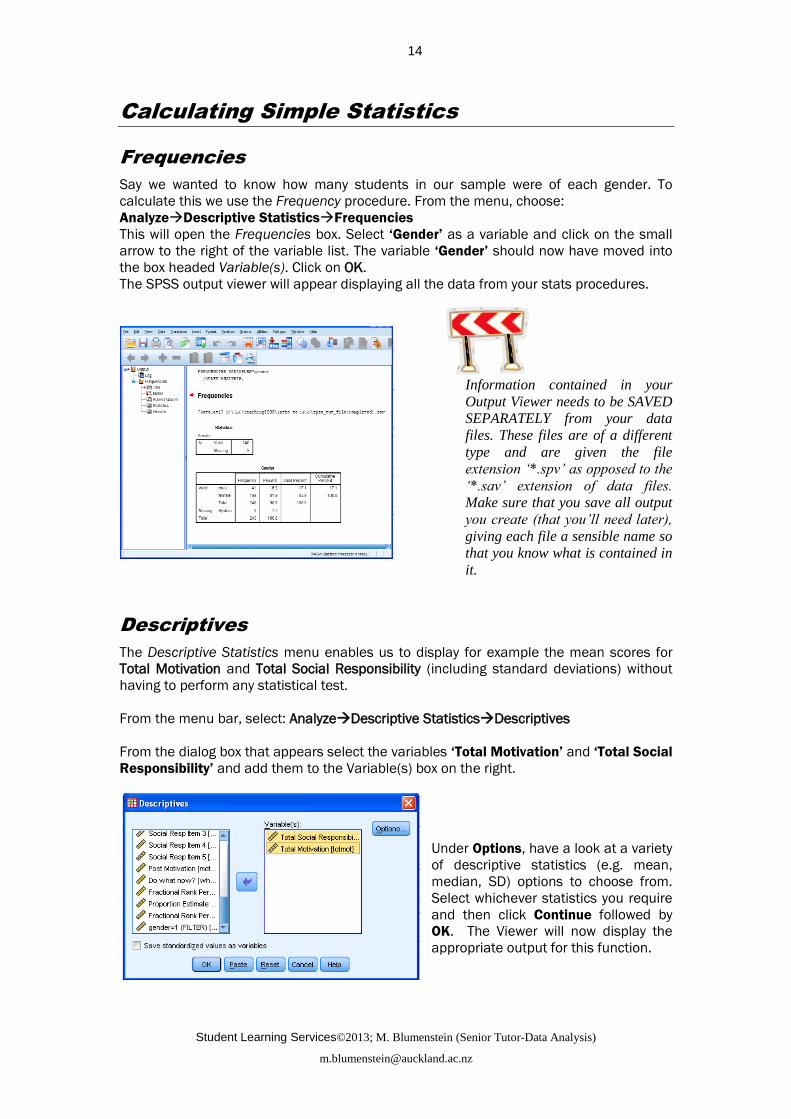
Descriptives
The Descriptive Statistics menu enables us to display for example the mean scores for
Total Motivation and Total Social Responsibility (including standard deviations) without
having to perform any statistical test.
From the menu bar, select: AnalyzeDescriptive StatisticsDescriptives
From the dialog box that appears select the variables ‘Total Motivation’ and ‘Total Social
Responsibility’ and add them to the Variable(s) box on the right.
Under Options, have a look at a variety
of descriptive statistics (e.g. mean,
median, SD) options to choose from.
Select whichever statistics you require
and then click Continue followed by
OK. The Viewer will now display the
appropriate output for this function.

Student Learning Services©2013; M. Blumenstein (Senior Tutor-Data Analysis)
15
Explore your data
The Explore procedure produces summary statistics and graphical displays, either for all
of your cases or separately for groups of cases. This procedure is used for data screening,
outlier identification, description, assumption checking, and characterizing differences
among subpopulations (groups of cases). Data screening may show that you have
unusual values, extreme values, gaps in the data, or other peculiarities. Exploring the
data can help to determine whether the statistical techniques that you are considering for
data analysis are appropriate. The exploration may indicate that you need to transform
the data if the technique requires a normal distribution. Or you may decide that you need
nonparametric tests.
We use the Explore procedure to look at the distribution of for example Total Motivation
scores (totmot) between males and females. From the menu bar choose:
AnalyzeDescriptive StatisticsExplore
This will open the Explore box. Select the variable ‘totmot’, and enter it into the
Dependent List box by clicking on the arrow to the left of the Dependent List box.
Select the variable ‘Gender’ and enter it into the Factor List box by clicking on the arrow
to the left of the Factor List box. For Display tick ‘both’
Click on Statistics and tick ‘Descriptives’ (95% confidence interval), continue. Click on
Plots and choose ‘Box Plots’ (Factor levels together), ‘Descriptive’ (stem and leaf plots;
histogram), tick ’Normality plots with tests (none)’, then click on continue then OK to run
the Explore procedure. The SPSS Viewer will display the appropriate output on
Descriptive statistics (take note of skewness and kurtosis to assess a possible
deviation from normal distribution)
Tests of Normality (Kolmorogov-Smirnov test)
Test of homogeneity of variance (Levene’s test)
Plots for exploring the distribution of your data for any deviation from normality
(histograms, box-and-whisker plots, Q-Q plots,
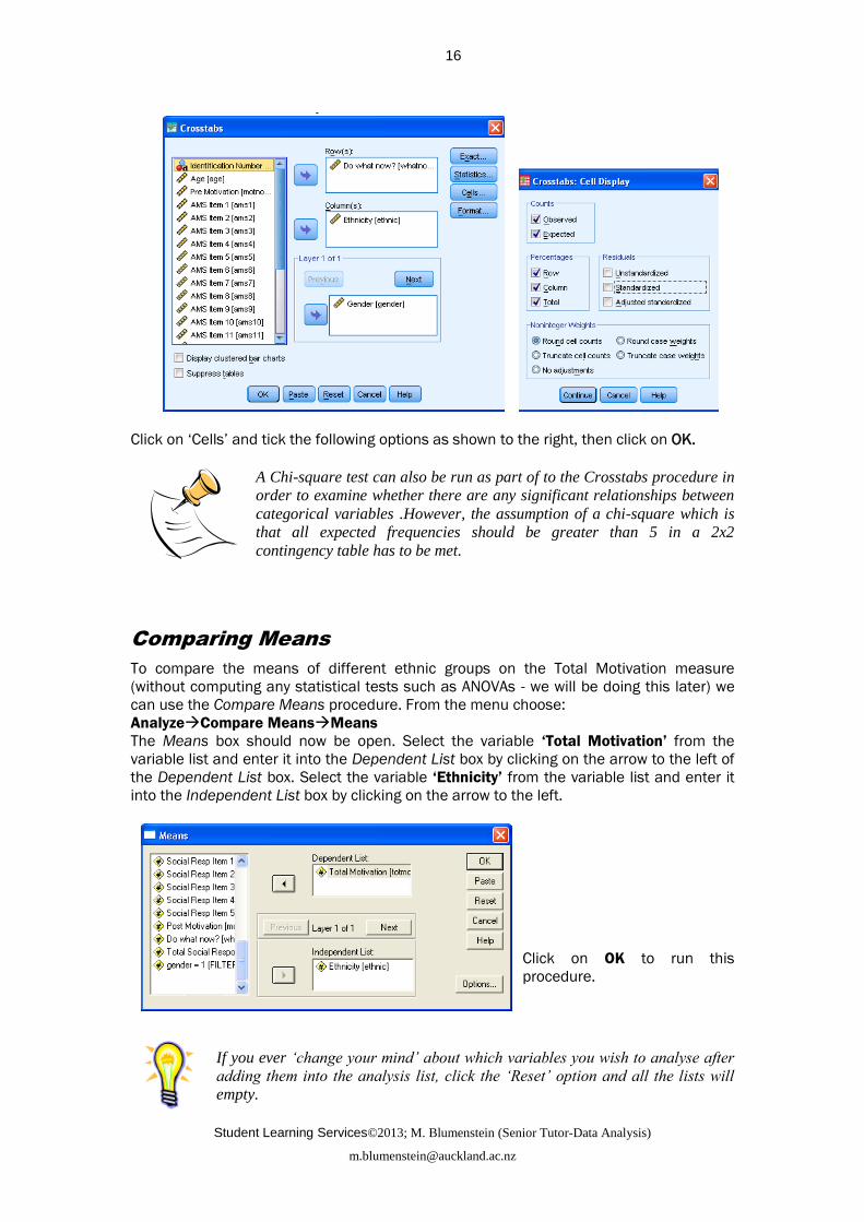
Crosstabulation
Crosstabs are commonly used to summarize categorical variables weighted on for
example frequencies. For example, using the present data, we might want to summarize
the number of cases for the activities in the variable whatnow by gender and ethnicity. To
run this procedure, from the menu bar choose: AnalyzeDescriptivesCrosstabs
Place the variable Do what now? into the Row(s) option and ‘Ethnicity’ into the Column(s)
option while Gender is entered as layer 1 of1 as shown below
Student Learning Services©2013; M. Blumenstein (Senior Tutor-Data Analysis)
16
Click on ‘Cells’ and tick the following options as shown to the right, then click on OK.
A Chi-square test can also be run as part of to the Crosstabs procedure in
order to examine whether there are any significant relationships between
categorical variables .However, the assumption of a chi-square which is
that all expected frequencies should be greater than 5 in a 2x2
contingency table has to be met.
Comparing Means
To compare the means of different ethnic groups on the Total Motivation measure
(without computing any statistical tests such as ANOVAs - we will be doing this later) we
can use the Compare Means procedure. From the menu choose:
AnalyzeCompare MeansMeans
The Means box should now be open. Select the variable ‘Total Motivation’ from the
variable list and enter it into the Dependent List box by clicking on the arrow to the left of
the Dependent List box. Select the variable ‘Ethnicity’ from the variable list and enter it
into the Independent List box by clicking on the arrow to the left.
Click on OK to run this
procedure.
If you ever ‘change your mind’ about which variables you wish to analyse after
adding them into the analysis list, click the ‘Reset’ option and all the lists will
empty.

Student Learning Services©2013; M. Blumenstein (Senior Tutor-Data Analysis)
17
Statistical Procedures
The following section provides examples of how to test for differences in means using t-
tests and one-way ANOVA. We will not be covering the theory of these tests in this
workshop.
One Sample T-Test
We want to compare a Total Motivation score from a previous study (the average there
was 62) with the total motivation scores of the whole group that was questioned in our
recent study. This can be done by using the one-sample t-test. Select:
AnalyzeCompare MeansOne Sample T-Test
From the dialogue box that appears, select ‘Total Motivation’ and add it across into the
Test Variable(s) box by clicking on the right-pointing arrow.
Enter 62 being the average score from a previous study into the box for Test Value.
Click on OK to run this
procedure.
Independent Groups T-Test
We have a suspicion that the Total Motivation score [totmot] of the males in our sample
are quite different from that of the females and decide to test for this. From the menu
bar, select: AnalyzeCompare MeansIndependent-Samples T-Test
From the dialogue box that appears, select totmot and add it across into the Test
Variable(s) box by clicking on the right-pointing arrow. Then select ‘Gender’ and add it
into the Grouping Variable box, once again by using the right-pointing arrow. The symbols
(? ?) will now appear after the gender variable (see screen picture below) as it will be
necessary to specify what values define your groups. To do this, click on the Define
Groups button. As we defined our groups as 1=male and 2=female, we will enter the
value 1 in the box for Group 1 and 2 in the box for Group 2. Follow this by clicking
Continue and then OK.

Student Learning Services©2013; M. Blumenstein (Senior Tutor-Data Analysis)
18
Paired Samples T-Test
Part of the questionnaire tested whether or not filling out a motivational survey affects
motivation levels by asking about students’ motivation both at the beginning and the end
of the questionnaire. We want to determine if this was the case by performing a paired-
samples t-test. From the menu bar, select:
AnalyzeCompare MeansPaired-Samples T-Test
From the dialogue box that appears, select ‘Pre Motivation’ and ‘Post Motivation’ and
add them both across into the Paired Variables box by clicking on the right-pointing arrow.
Then select OK.
If you want to make more than one comparison just enter the other pairs to be analysed
under Pair 2, 3, 4 etc
The t-test is an example of a parametric test: that is, it is assumed that your data
are normally distributed populations with the same variance. The non-
parametric equivalents do not make this assumption, for example the Wilcoxon
test (paired samples) or Mann Whitney test (independent samples).
Analysis of Variance (one-way ANOVA)
The One-Way ANOVA procedure produces a one-way analysis of variance for a
quantitative dependent variable (Dependent List) by a single independent variable
(Factor). Analysis of variance is used to test the hypothesis that several means are equal.
This technique is an extension of the two-sample t test.
In addition to determining that differences exist among the means, you may want to know
which means differ. There are two types of tests for comparing means: a priori contrasts
and post hoc tests. Contrasts are tests that are set up before running the experiment and
post hoc tests are run after the experiment has been conducted. Here we will focus on
post hoc tests.
We had four different ethnic groups in our sample and we wish to test whether or not
there is a difference in Total Motivation levels between these four groups.
From the menu bar select: AnalyseCompare MeansOne-Way ANOVA
Select ‘Ethnicity’ and add this into the Factor
box, add the ‘Total Motivation’ variable into
the Dependent List box.
Click on the OK button.

Student Learning Services©2013; M. Blumenstein (Senior Tutor-Data Analysis)
19
Post Hoc Tests
If the ANOVA is significant (p<0.05) we should find at least one significant difference
within the multiple comparisons. We therefore have to apply a PostHoc test to find out
where the difference lies. Bonferroni correction (conservative), Tukey tests for pairwise
comparisons, or the Dunnett test for comparisons against a baseline control group (e.g.
placebo group versus several drug treated groups) are commonly used.
To calculate post hoc test for our ANOVA, repeat the above procedure but click on the
Post Hoc button. For the present tutorial, choose the Bonferroni and Tukey options.
Click on Continue, then on OK.
Correlations
Correlations are used to test whether there is a relationship between one variable and
another. Beware, correlations cannot explain causality! From our survey data we may
wish to check how well age correlates with total motivation. In order to do this, from the
menu bar, select: AnalyzeCorrelateBivariate
Next, select the variables of ‘Age’
and ‘Total Motivation’ and add
these into the Variable(s) box as
shown below:
Click on OK.

Student Learning Services©2013; M. Blumenstein (Senior Tutor-Data Analysis)
20
SPSS will produce a table of correlations for you in the Output Viewer:
Correlations
Age Total Motivation
Age Pearson Correlation 1 -.038
Sig. (2-tailed) .552
N 243 243
Total Motivation Pearson Correlation -.038 1
Sig. (2-tailed) .552 N 243 243
From the Pearson Correlation we can see that motivation does not correlate with age (not
significant at 0.552 small coefficient at -0.038).
The Spearman Rank Correlation is used for not normally distributed data and nominal or
ordinal data sets.
Linear Regression
We will use Linear Regression to see if we can use a person’s ethnicity to predict how
motivated they are. From the menu bar select: AnalyzeRegressionLinear
The Linear Regression dialogue box will appear.
Move ‘Total Motivation’ into the Dependent box and ‘Ethnicity’ into the Independent(s)
box (see below):
Click on OK. The result is in the output viewer as shown below:
Model Summary
Model R R Square Adjusted R Square Std. Error of the Estimate
dimension0
1 .212a .045 .041 10.38117
a. Predictors: (Constant), Ethnicity
Only 4.5 % of the motivation can be predicted by ethnicity alone (R square of 0.045)
which means other factors play a much bigger role than ethnicity. Try the same
regression analysis with age as a predictor leaving Total Motivation [totmot] as a
dependent variable.

Student Learning Services©2013; M. Blumenstein (Senior Tutor-Data Analysis)
21
Chi-Square Test for Goodness of Fit
This test designed for for nominal data can be used to test the null hypothesis that our
sample population represents all ethnic groups at equal numbers. In other words, we
want to find out if some ethnic groups have significantly more representatives in our
sample than others. From the menu bar, select:
AnalyzeNonparametric TestsLegacy DialoguesChi-Square…
From the dialogue box that appears, select ‘Ethnicity’ and add it across to the Test
Variable List box by clicking on the right-pointing arrow. We are presuming that in our
study all categories (ie ethnic groups) should be equal in numbers.
Click on OK.
The output tell us that the Chi-square test is significant (p<0.05) which means that our
observed frequencies deviate from the expected numbers as can be seen in the table
below. Ethnicity
Observed N Expected N Residual
Pakeha 150 60.8 89.3 NZ Maori 28 60.8 -32.8 Pacific Islands 32 60.8 -28.8 Asian 33 60.8 -27.8 Total 243
Chi-square Test for Relatedness or Independence
We wish to determine if what respondents most felt like doing immediately after
completing the questionnaire is related to their gender.From the menu bar, select:
AnalyzeDescriptive StatisticsCrosstabs…
From the dialogue box that appears, select ‘Do What Now?’ and add it across to the
Row(s) box by clicking on the right-pointing arrow. Select ‘Gender’ and add it across to
the Column(s) box.

Student Learning Services©2013; M. Blumenstein (Senior Tutor-Data Analysis)
22
Click on the Statistics… button. Click on the Chi-square check box.
Click on Continue.
Click on the Cells… button. In the Counts box, click on the Observed and Expected check
boxes. In the Percentages box, click on the Row, Column and Total check boxes.
Click on Continue and then on OK.
All expected frequencies in a contingency table should be greater than 5 in
order to meet the assumptions of a Chi-square test otherwise the Chi-square
statistics is not valid. If you found an expected count lower than 5 than it is wise
to collect more data to try and boost the proportion of cases falling into each
category.
Reliability Analysis
In order to test whether questions that were asked in for example a survey are reliable i.e.
give consistent results if tested on different occasions by different testers or, as in our
case when attempting to generate a scale score by adding together the scores of a
number of variables, it is important to ensure that the questions are all measuring the
same thing. In the case of our example, the scale score is motivation. If some of the
questions are measuring something other than motivation, it does not make sense to
include them in this scale score. From the menu bar, select
AnalyzeScaleReliability Analysis
The Reliability Analysis dialogue box will appear.Select all the AMS items (1-12) in the
box on the left and move them across to the Items box on the right.

Student Learning Services©2013; M. Blumenstein (Senior Tutor-Data Analysis)
23
Click on the Statistics button
Ensure that Item, Scale, and Scale if item deleted are ticked.
Click Continue.
Click OK.
The following window will appear in the output_SPSS Viewer:
Reliability Statistics
Cronbach's Alpha N of Items
.763 12
Cronbach’s alpha is a model of internal consistency, based on the average inter-item
correlation. An acceptable value should be close to 0.8 (or above).
Creating Graphs
There are different ways of creating graphs in SPSS. There is a selection of different
graphs under the ‘Graphs’menu but graphs are options in analytical procedures as well
for example there is a Charts option in the Frequencies procedure and a Profile Plot
option in the ANOVA procedure. This tutorial focuses on producing graphs using Chart
Builder or Legacy Dialogs, which can be found on the SPSS menu bar under Graphs.
Creating a Bar Chart Summarizing Groups of Cases
From the menu choose : GraphsChart Builder (or Legacy Dialogs)
The Chart Builder box should now be open. It is important to set the measurement level
(nominal, ordinal, scalar) properly for each variable in ‘Variable View’. In addition assign
value labels if your variable has more than one category as for example in gender and
ethnicity.

Student Learning Services©2013; M. Blumenstein (Senior Tutor-Data Analysis)
24
From the gallery (tab) selection drag the bar chart into the chart preview window.
In the Element properties Box to the left of the chart builder window, click on Statistics
and select Mean and select ‘Display Error Bars’.
Into the X-Axis box underneath the graph drag ‘Ethnicity’ from the variable’s list
Into the Y-Axis box to the left of the graph drag ‘Total Motivation’ from the variable’s list.
Click on OK. The chart can now be seen in the SPSS Viewer. To copy the bar chart into a
new document (word file) for example your thesis or report, simply select the graph in
‘output viewer’ and use the copy and paste function from the ‘edit’ menu.
Creating a Clustered Bar Chart
From the menu choose: GraphsChart Builder (select the second bar chart picture and
drag into the chart preview window)
Drag the variable Do what now? into the X-box, and Total Motivation into the Y-box of the
graph. Drag Gender into the ‘Cluster on X’ box (here you can select a colour or a pattern
for your bars; I have selected ‘pattern’).
In the ‘Element Properties’ box under ‘Statistics’ select Mean and tick the ‘Display Error
bars’ box, then ‘click on ‘Apply’

Student Learning Services©2013; M. Blumenstein (Senior Tutor-Data Analysis)
25
Click on OK. The chart can now be seen in the SPSS Statistics Viewer. Use ‘copy and
paste’ function to transfer the graph into a new document.
Editing Charts
To make changes to a chart, double click on the chart while being in the output viewer.
This will open the Chart Editor. The menu bar of this window gives a variety of options of
features you may wish to alter. For example, we may wish to add a more descriptive title
to our graph. From the Chart Editor menu bar, select: OptionsTitle
You can now type in a more appropriate title for the graph. An alternative to the menu
bar is to double click on the feature that you wish to change e.g. the axes – try this now
and see what happens.
To make further changes to the graph, try using the buttons available on the Chart Editor
toolbar.
To change something in the Chart Editor it must be selected first. For
example, to change the colour on the bars of a bar graph, you must first
select the bars by clicking on them once and then choosing to change the
colour.
Chart Templates
Once we have a chart looking just as we want it, we do not want to have to change every
chart we create into that format. For example, if we are writing a manuscript for
publishing in a journal that needs to be in APA format it may take a lot of time to transfer
all our charts into this form.
Once you complete a chart that completes your format, from the menu bar in the Chart
Editor, choose: FileSave Chart Template.....
Enter a name for your template, choose a location ie desktop or ‘my documents’ and click
Save (your template will be given an *.sgt extension).
When you need to create another graph using this style, produce the graph first then in
chart editor click on: File Apply Chart Template and locate your previously saved
template, then click on OK.
Student Learning Services©2013; M. Blumenstein (Senior Tutor-Data Analysis)
26
Running Procedures and Getting Help
You are now at a point where you could probably run any analysis you wanted in SPSS, as
all the procedures work the same way as those described above. The two most frequently
asked questions, however, regarding how to run procedures are discussed below:
Firstly, how do I decide which procedure to actually run ? This will require some basic
statistical knowledge. If you are unsure which test to use, you might like to have a play
with the Statistics Coach, which can be accessed from the Help menu in SPSS. This
‘Coach’ will guide you through a series of questions regarding your data and the
questions you want answered from your data, and then suggest a possible statistical
technique for this.
Secondly, how do I define my variables to add across into the analyses boxes? Knowing
your independent variables from your dependent variables will be a big help here. Note
that in some dialog boxes SPSS refers to the independent variable as a ‘factor’,
‘covariate’, or ‘grouping variable’ and the dependent variable as a ‘test variable. If you’ve
made a mistake you can re-run the procedure by re-calling your most recently used
analysis by clicking on the ‘Dialog Recall’ button located on the toolbar:
Users are often unsure as to what the various terms and options mean in the dialog
boxes. In nearly all of the dialog boxes in SPSS, right clicking over a term (i.e. clicking the
right mouse button instead of the left) will bring up a definition for you – very handy!!
Further reading
1. Andy Field (2009) Discovering statistics using SPSS. London: SAGE
2. Paul R Kinnear & Colin D Gray (2009) SPSS 16 made simple. Hove, East Sussex:
Psychology Press
3. Julie Pallant (2011) SPSS Survival Guide, 4th edition. Crows Nest, NSW, Australia:
Allen&Unwin.
Working With Output
By this point of our tutorial we have created a lot of output in our Output Viewer. You may
have noticed that down the left hand side of your Output Viewer there is a list of all the
output you have created. You can use this outline to navigate through your output and
control the output display. You need to save your output file separately from any changes
made to your data set!
You can collapse or expand items by clicking on the “-“ or “+” sign next to the item as
appropriate. You can also delete items of output by selecting them on the left-hand side
and pressing the delete key.
Student Learning Services©2013; M. Blumenstein (Senior Tutor-Data Analysis)
27
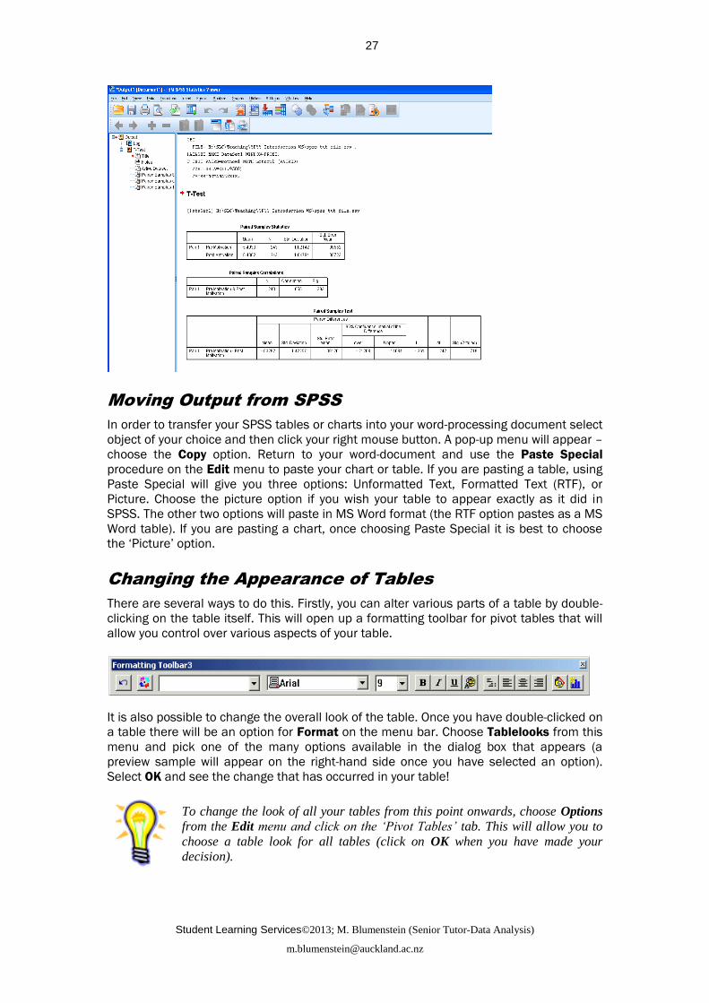
Moving Output from SPSS
In order to transfer your SPSS tables or charts into your word-processing document select
object of your choice and then click your right mouse button. A pop-up menu will appear –
choose the Copy option. Return to your word-document and use the Paste Special
procedure on the Edit menu to paste your chart or table. If you are pasting a table, using
Paste Special will give you three options: Unformatted Text, Formatted Text (RTF), or
Picture. Choose the picture option if you wish your table to appear exactly as it did in
SPSS. The other two options will paste in MS Word format (the RTF option pastes as a MS
Word table). If you are pasting a chart, once choosing Paste Special it is best to choose
the ‘Picture’ option.
Changing the Appearance of Tables
There are several ways to do this. Firstly, you can alter various parts of a table by double-
clicking on the table itself. This will open up a formatting toolbar for pivot tables that will
allow you control over various aspects of your table.
It is also possible to change the overall look of the table. Once you have double-clicked on
a table there will be an option for Format on the menu bar. Choose Tablelooks from this
menu and pick one of the many options available in the dialog box that appears (a
preview sample will appear on the right-hand side once you have selected an option).
Select OK and see the change that has occurred in your table!
To change the look of all your tables from this point onwards, choose Options
from the Edit menu and click on the ‘Pivot Tables’ tab. This will allow you to
choose a table look for all tables (click on OK when you have made your
decision).
Student Learning Services©2013; M. Blumenstein (Senior Tutor-Data Analysis)
28
Working with SPSS Statistics Syntax
In early versions of SPSS, it was necessary to write syntax in order to analyse your data.
SPSS Syntax is a control language, and is similar in concept to the programming code
written in SAS. While we no longer need syntax to operate SPSS, it has remained a
feature of the software and can be very useful, for example:
To run a common set of commands without choosing all the options over and over
again from the dialog boxes.
To re-run a complicated (or lengthy) set of procedures with just a minor change
from your earlier analysis – if you have saved your syntax, the procedure can be
re-run with your minor changes simply by one click of a button.
To provide a ‘record’ of your analysis in terms of either accountability or for
documentation purposes about the procedures used.
Finally, some SPSS functions are actually not available from the menu options and
can only be accessed via syntax, for example if you need to break down the
interactions of independent variables after doing a factorial ANOVA (simple
effects analysis).
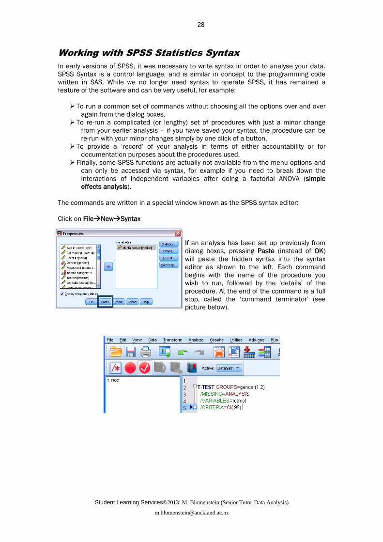
The commands are written in a special window known as the SPSS syntax editor:
Click on FileNewSyntax
If an analysis has been set up previously from
dialog boxes, pressing Paste (instead of OK)
will paste the hidden syntax into the syntax
editor as shown to the left. Each command
begins with the name of the procedure you
wish to run, followed by the ‘details’ of the
procedure. At the end of the command is a full
stop, called the ‘command terminator’ (see
picture below).

Student Learning Services©2013; M. Blumenstein (Senior Tutor-Data Analysis)
29
Motivation Survey
Please complete the following:
ID#
Age Gender Ethnicity
For the remaining questions, please circle the response that best fits you:
MOTNOW1How motivated do you feel towards your University studies right now?
not very motivated very motivated
1 2 3 4 5 6 7
Using the scale below, indicate to what extent each of the following items presently
corresponds to one of the reasons why you go to University.
Does not
correspond at all
Corresponds
moderately
Corresponds
exactly
1 2 3 4 5 6 7
Motivation Items AMS 1 - 12
1. Because with only a high-school qualification I would
not find a high-paying job later on.
1
2
3
4
5
6
7
2. Because I experience pleasure and satisfaction while
learning new things.
1
2
3
4
5
6
7
3. For the intense feelings I experience when I am
communicating my own ideas to others.
1
2
3
4
5
6
7
4. In order to obtain a more prestigious job later on. 1 2 3 4 5 6 7
5. I once had good reasons for going to University;
however, now I wonder whether I should continue.
1
2
3
4
5
6
7
6. For the pleasure that I experience while I am
surpassing myself in one of my personal
accomplishments.
1
2
3
4
5
6
7
Student Learning Services©2013; M. Blumenstein (Senior Tutor-Data Analysis)
30
7. Because I want to have ‘the good life’ later on. 1 2 3 4 5 6 7
8. For the pleasure that I experience when I feel
completely absorbed by what certain authors have
written.
1
2
3
4
5
6
7
9. For the satisfaction I feel when I am in the process of
accomplishing difficult activities.
1
2
3
4
5
6
7
10. Because my studies allow me to continue to learn
about many things that interest me.
1
2
3
4
5
6
7
11. For the "high" feeling that I experience while reading
about various interesting subjects.
1
2
3
4
5
6
7
12. Because University allows me to experience a
personal satisfaction in my quest for excellence in my
studies.
1
2
3
4
5
6
7
Please indicate to what extent each of the following statements are true of you,
1 = not at all true of me, and 5 = very true of me.
Social Responsibility Items SR1 - 5
1. I try to think how my behaviour will affect other students completing
the same course as me.
1 2 3 4 5
2. I like to keep promises that I have made to other people in my course. 1 2 3 4 5
3. I try to do what my lecturer/supervisor asks me. 1 2 3 4 5
4. I try to share what I have learnt with other people in the same course
as me.
1 2 3 4 5
5. I like to keep quiet when other people are trying to study. 1 2 3 4 5
MOTNOW2 Having completed this questionnaire, how motivated do you feel towards your
University studies now?
not very motivated very motivated
1 2 3 4 5 6 7
WHATNOW Having completed this questionnaire, what do you most feel like doing?
1 = Study-related work 2 = Watching TV
3 = Doing nothing 4 = Going down to the pub