Introduction to Prolog Programming - NTUAglotta.ntua.gr/courses/Technoglossia/Logic/prolog.pdf · And Introduction to Prolog Programming 3 of bigger. Animal X is bigger than animal

Institute for Logic,Language and Computation

Lecture Notes

An Introduction to Prolog Programming

Ulle Endriss

Universiteit van Amsterdam

c© by Ulle Endriss, University of Amsterdam (Email: [email protected])

Version: 1 September 2013

mailto:[email protected]?subject=Prolog Notes

Preface

These lecture notes introduce the declarative programming language Prolog. The em-

phasis is on learning how to program, rather than on the theory of logic programming.

Nevertheless, a short chapter on the logic foundations of Prolog is included as well.

All examples have been tested using SWI-Prolog (www.swi-prolog.org) and can be ex-

pected to work equally well with most other Prolog systems. These notes have originally

been developed for a course I taught at King’s College London in 1999 and 2000.

Amsterdam, August 2005 U.E.

The present version corrects a number of minor errors in the text, most of which

have been pointed out to me by students following a number of courses I have given at

the University of Amsterdam since 2005.

Amsterdam, September 2013 U.E.

iii

http://www.swi-prolog.org

Contents

1 The Basics 1

1.1 Getting Started: An Example . . . . . . . . . . . . . . . . . . . . . . . . . 1

1.2 Prolog Syntax . . . . . . . . . . . . . . . . . . . . . . . . . . . . . . . . . . 4

1.2.1 Terms . . . . . . . . . . . . . . . . . . . . . . . . . . . . . . . . . . 4

1.2.2 Clauses, Programs and Queries . . . . . . . . . . . . . . . . . . . . 5

1.2.3 Some Built-in Predicates . . . . . . . . . . . . . . . . . . . . . . . 6

1.3 Answering Queries . . . . . . . . . . . . . . . . . . . . . . . . . . . . . . . 8

1.3.1 Matching . . . . . . . . . . . . . . . . . . . . . . . . . . . . . . . . 8

1.3.2 Goal Execution . . . . . . . . . . . . . . . . . . . . . . . . . . . . . 10

1.4 A Matter of Style . . . . . . . . . . . . . . . . . . . . . . . . . . . . . . . . 11

1.5 Exercises . . . . . . . . . . . . . . . . . . . . . . . . . . . . . . . . . . . . 12

2 List Manipulation 15

2.1 Notation . . . . . . . . . . . . . . . . . . . . . . . . . . . . . . . . . . . . . 15

2.2 Head and Tail . . . . . . . . . . . . . . . . . . . . . . . . . . . . . . . . . . 15

2.3 Some Built-in Predicates for List Manipulation . . . . . . . . . . . . . . . 18

2.4 Exercises . . . . . . . . . . . . . . . . . . . . . . . . . . . . . . . . . . . . 19

3 Arithmetic Expressions 21

3.1 The is-Operator for Arithmetic Evaluation . . . . . . . . . . . . . . . . . 21

3.2 Predefined Arithmetic Functions and Relations . . . . . . . . . . . . . . . 22

3.3 Exercises . . . . . . . . . . . . . . . . . . . . . . . . . . . . . . . . . . . . 23

4 Operators 27

4.1 Precedence and Associativity . . . . . . . . . . . . . . . . . . . . . . . . . 27

4.2 Declaring Operators with op/3 . . . . . . . . . . . . . . . . . . . . . . . . 30

4.3 Exercises . . . . . . . . . . . . . . . . . . . . . . . . . . . . . . . . . . . . 31

5 Backtracking, Cuts and Negation 35

5.1 Backtracking and Cuts . . . . . . . . . . . . . . . . . . . . . . . . . . . . . 35

5.1.1 Backtracking Revisited . . . . . . . . . . . . . . . . . . . . . . . . . 35

5.1.2 Problems with Backtracking . . . . . . . . . . . . . . . . . . . . . . 36

5.1.3 Introducing Cuts . . . . . . . . . . . . . . . . . . . . . . . . . . . . 37

v

vi Contents

5.1.4 Problems with Cuts . . . . . . . . . . . . . . . . . . . . . . . . . . 40

5.2 Negation as Failure . . . . . . . . . . . . . . . . . . . . . . . . . . . . . . . 41

5.2.1 The Closed World Assumption . . . . . . . . . . . . . . . . . . . . 41

5.2.2 The \+-Operator . . . . . . . . . . . . . . . . . . . . . . . . . . . . 42

5.3 Disjunction . . . . . . . . . . . . . . . . . . . . . . . . . . . . . . . . . . . 43

5.4 Example: Evaluating Logic Formulas . . . . . . . . . . . . . . . . . . . . . 44

5.5 Exercises . . . . . . . . . . . . . . . . . . . . . . . . . . . . . . . . . . . . 46

6 Logic Foundations of Prolog 49

6.1 Translation of Prolog Clauses into Formulas . . . . . . . . . . . . . . . . . 49

6.2 Horn Formulas and Resolution . . . . . . . . . . . . . . . . . . . . . . . . 51

6.3 Exercises . . . . . . . . . . . . . . . . . . . . . . . . . . . . . . . . . . . . 53

A Recursive Programming 55

A.1 Complete Induction . . . . . . . . . . . . . . . . . . . . . . . . . . . . . . 55

A.2 The Recursion Principle . . . . . . . . . . . . . . . . . . . . . . . . . . . . 56

A.3 What Problems to Solve . . . . . . . . . . . . . . . . . . . . . . . . . . . . 57

A.4 Debugging . . . . . . . . . . . . . . . . . . . . . . . . . . . . . . . . . . . . 57

Index 59

Chapter 1

The Basics

Prolog (programming in log ic) is one of the most widely used programming languages in

artificial intelligence research. As opposed to imperative languages such as C or Java (the

latter of which also happens to be object-oriented) it is a declarative programming lan-

guage. That means, when implementing the solution to a problem, instead of specifying

how to achieve a certain goal in a certain situation, we specify what the situation (rules

and facts) and the goal (query) are and let the Prolog interpreter derive the solution for

us. Prolog is very useful in some problem areas, such as artificial intelligence, natural

language processing, databases, . . . , but pretty useless in others, such as graphics or

numerical algorithms.

By following this course, you will learn how to use Prolog as a programming language

to solve practical problems in computer science and artificial intelligence. You will also

learn how the Prolog interpreter actually works. The latter will include an introduction

to the logical foundations of the Prolog language.

These notes cover the most important Prolog concepts you need to know about, but

it is certainly worthwhile to also have a look at the literature. The following three are

well-known titles, but you may also consult any other textbook on Prolog.

• I. Bratko. Prolog Programming for Artificial Intelligence. 4th edition, Addison-

Wesley Publishers, 2012.

• F. W. Clocksin and C. S. Mellish. Programming in Prolog. 5th edition, Springer-

Verlag, 2003.

• L. Sterling and E. Shapiro. The Art of Prolog. 2nd edition, MIT Press, 1994.

1.1 Getting Started: An Example

In the introduction it has been said that Prolog is a declarative (or descriptive) language.

Programming in Prolog means describing the world. Using such programs means asking

Prolog questions about the previously described world. The simplest way of describing

the world is by stating facts, like this one:

1

2 Chapter 1. The Basics

bigger(elephant, horse).

This states, quite intuitively, the fact that an elephant is bigger than a horse. (Whether

the world described by a Prolog program has anything to do with our real world is, of

course, entirely up to the programmer.) Let’s add a few more facts to our little program:


bigger(horse, donkey).

bigger(donkey, dog).

bigger(donkey, monkey).

This is a syntactically correct program, and after having compiled it we can ask the Prolog

system questions (or queries in proper Prolog-jargon) about it. Here’s an example:

?- bigger(donkey, dog).

Yes

The query bigger(donkey, dog) (i.e., the question “Is a donkey bigger than a dog?”)

succeeds, because the fact bigger(donkey, dog) has previously been communicated to

the Prolog system. Now, is a monkey bigger than an elephant?

?- bigger(monkey, elephant).

No

No, it’s not. We get exactly the answer we expected: the corresponding query, namely

bigger(monkey, elephant) fails. But what happens when we ask the other way round?

?- bigger(elephant, monkey).

No

According to this elephants are not bigger than monkeys. This is clearly wrong as far as

our real world is concerned, but if you check our little program again, you will find that

it says nothing about the relationship between elephants and monkeys. Still, we know

that if elephants are bigger than horses, which in turn are bigger than donkeys, which in

turn are bigger than monkeys, then elephants also have to be bigger than monkeys. In

mathematical terms: the bigger-relation is transitive. But this has also not been defined

in our program. The correct interpretation of the negative answer Prolog has given is the

following: from the information communicated to the system it cannot be proved that

an elephant is bigger than a monkey.

If, however, we would like to get a positive reply for a query like bigger(elephant,

monkey), we have to provide a more accurate description of the world. One way of doing

this would be to add the remaining facts, such as bigger(elephant, monkey), to our

program. For our little example this would mean adding another 5 facts. Clearly too

much work and probably not too clever anyway.

The far better solution would be to define a new relation, which we will call

is_bigger, as the transitive closure (don’t worry if you don’t know what that means)

Ulle Endriss. And Introduction to Prolog Programming 3

of bigger. Animal X is bigger than animal Y either if this has been stated as a fact or if

there is an animal Z for which it has been stated as a fact that animal X is bigger than

animal Z and it can be shown that animal Z is bigger than animal Y. In Prolog such

statements are called rules and are implemented like this:

is_bigger(X, Y) :- bigger(X, Y).

is_bigger(X, Y) :- bigger(X, Z), is_bigger(Z, Y).

In these rules :- means something like “if” and the comma between the two terms

bigger(X, Z) and is_bigger(Z, Y) stands for “and”. X, Y, and Z are variables, which

in Prolog is indicated by using capital letters.

You can think of the the bigger-facts as data someone has collected by browsing

through the local zoo and comparing pairs of animals. The implementation of is_bigger,

on the other hand, could have been provided by a knowledge engineer who may not

know anything at all about animals, but understands the general concept of something

being bigger than something else and thereby has the ability to formulate general rules

regarding this relation. If from now on we use is_bigger instead of bigger in our

queries, the program will work as intended:

?- is_bigger(elephant, monkey).

Yes

Prolog still cannot find the fact bigger(elephant, monkey) in its database, so it tries

to use the second rule instead. This is done by matching the query with the head of the

rule, which is is_bigger(X, Y). When doing so the two variables get instantiated: X =

elephant and Y = monkey. The rule says that in order to prove the goal is_bigger(X,

Y) (with the variable instantiations that’s equivalent to is_bigger(elephant, monkey))

Prolog has to prove the two subgoals bigger(X, Z) and is_bigger(Z, Y), again with

the same variable instantiations. This process is repeated recursively until the facts

that make up the chain between elephant and monkey are found and the query finally

succeeds. How this goal execution as well as term matching and variable instantiation

really work will be examined in more detail in Section 1.3.

Of course, we can do slightly more exiting stuff than just asking yes/no-questions.

Suppose we want to know, what animals are bigger than a donkey? The corresponding

query would be:

?- is_bigger(X, donkey).

Again, X is a variable. We could also have chosen any other name for it, as long as it

starts with a capital letter. The Prolog interpreter replies as follows:


X = horse

Horses are bigger than donkeys. The query has succeeded, but in order to allow it to

succeed Prolog had to instantiate the variable X with the value horse. If this makes us


happy already, we can press Return now and that’s it. In case we want to find out if

there are more animals that are bigger than the donkey, we can press the semicolon key,

which will cause Prolog to search for alternative solutions to our query. If we do this

once, we get the next solution X = elephant: elephants are also bigger than donkeys.

Pressing semicolon again will return a No, because there are no more solutions:


X = horse ;

X = elephant ;

No

There are many more ways of querying the Prolog system about the contents of its

database. As a final example we ask whether there is an animal X that is both smaller

than a donkey and bigger than a monkey:

?- is_bigger(donkey, X), is_bigger(X, monkey).

No

The (correct) answer is No. Even though the two single queries is_bigger(donkey, X)

and is_bigger(X, monkey) would both succeed when submitted on their own, their

conjunction (represented by the comma) does not.

This section has been intended to give you a first impression of Prolog programming.

The next section provides a more systematic overview of the basic syntax.

There are a number of Prolog systems around that you can use. How to start a

Prolog session may differ slightly from one system to the next, but it should not be too

difficult to find out by consulting the user manual of your system. The examples in these

notes have all been generated using SWI-Prolog (in its 1999 incarnation, with only a few

minor adjustments made later on).1

1.2 Prolog Syntax

This section describes the most basic features of the Prolog programming language.

1.2.1 Terms

The central data structure in Prolog is that of a term. There are terms of four kinds:

atoms, numbers, variables, and compound terms. Atoms and numbers are sometimes

grouped together and called atomic terms.

1One difference between “classical” Prolog and more recent versions of SWI-Prolog is that the latter

reports true rather than Yes when a query succeeds and false rather than No when a query fails. There

also a a few other very minor differences in how modern SWI-Prolog responds to queries. If you are

interested in the finer subtleties of this matter, search the Internet for “Prolog toplevel”.


Atoms. Atoms are usually strings made up of lower- and uppercase letters, digits, and

the underscore, starting with a lowercase letter. The following are all valid Prolog atoms:

elephant, b, abcXYZ, x_123, another_pint_for_me_please

On top of that also any series of arbitrary characters enclosed in single quotes denotes

an atom.

’This is also a Prolog atom.’

Finally, strings made up solely of special characters like + - * = < > : & (check the

manual of your Prolog system for the exact set of these characters) are also atoms.

Examples:

+, ::, <------>, ***

Numbers. All Prolog implementations have an integer type: a sequence of digits,

optionally preceded by a - (minus). Some also support floats. Check the manual for

details.

Variables. Variables are strings of letters, digits, and the underscore, starting with a

capital letter or an underscore. Examples:

X, Elephant, _4711, X_1_2, MyVariable, _

The last one of the above examples (the single underscore) constitutes a special case.

It is called the anonymous variable and is used when the value of a variable is of no

particular interest. Multiple occurrences of the anonymous variable in one expression

are assumed to be distinct, i.e., their values don’t necessarily have to be the same. More

on this later.

Compound terms. Compound terms are made up of a functor (a Prolog atom) and

a number of arguments (Prolog terms, i.e., atoms, numbers, variables, or other com-

pound terms) enclosed in parentheses and separated by commas. The following are some

examples for compound terms:

is_bigger(horse, X), f(g(X, _), 7), ’My Functor’(dog)

It’s important not to put any blank characters between the functor and the opening

parentheses, or Prolog won’t understand what you’re trying to say. In other places,

however, spaces can be very helpful for making programs more readable.

The sets of compound terms and atoms together form the set of Prolog predicates.

A term that doesn’t contain any variables is called a ground term.

1.2.2 Clauses, Programs and Queries

In the introductory example we have already seen how Prolog programs are made up of

facts and rules. Facts and rules are also called clauses.


Facts. A fact is a predicate followed by a full stop. Examples:

bigger(whale, _).

life_is_beautiful.

The intuitive meaning of a fact is that we define a certain instance of a relation as being

true.

Rules. A rule consists of a head (a predicate) and a body. (a sequence of predicates

separated by commas). Head and body are separated by the sign :- and, like every

Prolog expression, a rule has to be terminated by a full stop. Examples:

is_smaller(X, Y) :- is_bigger(Y, X).

aunt(Aunt, Child) :-

sister(Aunt, Parent),

parent(Parent, Child).

The intuitive meaning of a rule is that the goal expressed by its head is true, if we (or

rather the Prolog system) can show that all of the expressions (subgoals) in the rule’s

body are true.

Programs. A Prolog program is a sequence of clauses.

Queries. After compilation a Prolog program is run by submitting queries to the in-

terpreter. A query has the same structure as the body of a rule, i.e., it is a sequence of

predicates separated by commas and terminated by a full stop. They can be entered at

the Prolog prompt, which in most implementations looks something like this: ?-. When

writing about queries we often include the ?-. Examples:

?- is_bigger(elephant, donkey).

?- small(X), green(X), slimy(X).

Intuitively, when submitting a query like the last example, we ask Prolog whether all its

predicates are provably true, or in other words whether there is an X such that small(X),

green(X), and slimy(X) are all true.

1.2.3 Some Built-in Predicates

What we have seen so far is already enough to write simple programs by defining pred-

icates in terms of facts and rules, but Prolog also provides a range of useful built-in

predicates. Some of them will be introduced in this section; all of them should be ex-

plained in the user manual of your Prolog system.

Built-ins can be used in a similar way as user-defined predicates. The important

difference between the two is that a built-in predicate is not allowed to appear as the

principal functor in a fact or the head of a rule. This must be so, because using them in

such a position would effectively mean changing their definition.


Equality. Maybe the most important built-in predicate is = (equality). Instead of

writing expressions such as =(X, Y), we usually write more conveniently X = Y. Such a

goal succeeds, if the terms X and Y can be matched. This will be made more precise in

Section 1.3.

Guaranteed success and certain failure. Sometimes it can be useful to have predi-

cates that are known to either fail or succeed in any case. The predicates fail and true

serve exactly this purpose. Some Prolog systems also provide the predicate false, with

exactly the same functionality as fail.

Consulting program files. Program files can be compiled using the predicate

consult/1.2 The argument has to be a Prolog atom denoting the program file you

want to compile. For example, to compile the file big-animals.pl submit the following

query to Prolog:

?- consult(’big-animals.pl’).

If the compilation is successful, Prolog will reply with Yes. Otherwise a list of errors will

be displayed.

Output. If besides Prolog’s replies to queries you wish your program to have further

output you can use the write/1 predicate. The argument can be any valid Prolog term.

In the case of a variable its value will get printed to the screen. Execution of the predicate

nl/0 causes the system to skip a line. Here are two examples:

?- write(’Hello World!’), nl.

Hello World!

Yes

?- X = elephant, write(X), nl.

elephant

X = elephant

Yes

In the second example, first the variable X is bound to the atom elephant and then the

value of X, i.e., elephant, is written on the screen using the write/1 predicate. After

skipping to a new line, Prolog reports the variable binding(s), i.e., X = elephant.

Checking the type of a Prolog term. There are a number of built-in predicates

available that can be used to check the type of a given Prolog term. Here are some

examples:

2 The /1 is used to indicate that this predicate takes one argument.


?- atom(elephant).

Yes

?- atom(Elephant).

No

?- X = f(mouse), compound(X).

X = f(mouse)

Yes

The last query succeeds, because the variable X is bound to the compound term f(mouse)

at the time the subgoal compound(X) is being executed.

Help. Most Prolog systems also provide a help function in the shape of a predicate,

usually called help/1. Applied to a term (like the name of a built-in predicate) the

system will display a short description, if available. Example:

?- help(atom).

atom(+Term)

Succeeds if Term is bound to an atom.

1.3 Answering Queries

We have mentioned the issue of term matching before in these notes. This concept is

crucial to the way Prolog replies to queries, so we present it before describing what

actually happens when a query is processed (or more generally speaking: when a goal is

executed).

1.3.1 Matching

Two terms are said to match if they are either identical or if they can be made identical

by means of variable instantiation. Instantiating a variable means assigning it a fixed

value. Two free variables also match, because they could be instantiated with the same

ground term.

It is important to note that the same variable has to be instantiated with the same

value throughout an expression. The only exception to this rule is the anonymous vari-

able _, which is considered to be unique whenever it occurs.

We give some examples. The terms is_bigger(X, dog) and is_bigger(elephant,

dog) match, because the variable X can be instantiated with the atom elephant. We

could test this in the Prolog interpreter by submitting the corresponding query to which

Prolog would react by listing the appropriate variable instantiations:

?- is_bigger(X, dog) = is_bigger(elephant, dog).


X = elephant

Yes

The following is an example for a query that doesn’t succeed, because X cannot match

with 1 and 2 at the same time.

?- p(X, 2, 2) = p(1, Y, X).

No

If, however, instead of X we use the anonymous variable _, matching is possible, because

every occurrence of _ represents a distinct variable. During matching Y is instantiated

with 2:

?- p(_, 2, 2) = p(1, Y, _).

Y = 2

Yes

Another example for matching:

?- f(a, g(X, Y)) = f(X, Z), Z = g(W, h(X)).

X = a

Y = h(a)

Z = g(a, h(a))

W = a

Yes

So far so good. But what happens, if matching is possible even though no specific variable

instantiation has to be enforced (like in all previous examples)? Consider the following

query:

?- X = my_functor(Y).

X = my_functor(_G177)

Y = _G177

Yes

In this example matching succeeds, because X could be a compound term with the functor

my_functor and a non-specified single argument. Y could be any valid Prolog term, but

it has to be the same term as the argument inside X. In Prolog’s output this is denoted

through the use of the variable _G177. This variable has been generated by Prolog during

execution time. Its particular name, _G177 in this case, may be different every time the

query is submitted.

In fact, what the output for the above example will look like exactly will depend on the

Prolog system you use. For instance, some systems will avoid introducing a new variable

(here _G177) and instead simply report the variable binding as X = my_functor(Y).


1.3.2 Goal Execution

Submitting a query means asking Prolog to try to prove that the statement(s) implied

by the query can be made true provided the right variable instantiations are made. The

search for such a proof is usually referred to as goal execution. Each predicate in the query

constitutes a (sub)goal, which Prolog tries to satisfy one after the other. If variables are

shared between several subgoals their instantiations have to be the same throughout the

entire expression.

If a goal matches with the head of a rule, the respective variable instantiations are

made inside the rule’s body, which then becomes the new goal to be satisfied. If the body

consists of several predicates the goal is again split into subgoals to be executed in turn.

In other words, the head of a rule is considered provably true, if the conjunction of all

its body-predicates are provably true. If a goal matches with a fact in our program, the

proof for that goal is complete and the variable instantiations made during matching are

communicated back to the surface. Note that the order in which facts and rules appear

in our program is important here. Prolog will always try to match its current goal with

the first possible fact or rule-head it can find.

If the principal functor of a goal is a built-in predicate the associated action is exe-

cuted whilst the goal is being satisfied. For example, as far as goal execution is concerned

the predicate

write(’Hello World!’)

will simply succeed, but at the same time it will also print the words Hello World! on

the screen.

As mentioned before, the built-in predicate true will always succeed (without any

further side-effects), whereas fail will always fail.

Sometimes there is more than one way of satisfying the current goal. Prolog chooses

the first possibility (as determined by the order of clauses in a program), but the fact

that there are alternatives is recorded. If at some point Prolog fails to prove a certain

subgoal, the system can go back and try an alternative way of executing the previous

goal. This process is known as backtracking.

We shall exemplify the process of goal execution by means of the following famous

argument:

All men are mortal.

Socrates is a man.

Hence, Socrates is mortal.

In Prolog terms, the first statement represents a rule: X is mortal, if X is a man (for all

X). The second one constitutes a fact: Socrates is a man. This can be implemented in

Prolog as follows:

mortal(X) :- man(X).

man(socrates).


Note that X is a variable, whereas socrates is an atom. The conclusion of the argument,

“Socrates is mortal”, can be expressed through the predicate mortal(socrates). After

having consulted the above program we can submit this predicate to Prolog as a query,

which will cause the following reaction:

?- mortal(socrates).

Yes

Prolog agrees with our own logical reasoning. Which is nice. But how did it come to its

conclusion? Let’s follow the goal execution step by step.

(1) The query mortal(socrates) is made the initial goal.

(2) Scanning through the clauses of our program, Prolog tries to match

mortal(socrates) with the first possible fact or head of rule. It finds mortal(X),

the head of the first (and only) rule. When matching the two terms the instantia-

tion X = socrates needs to be made.

(3) The variable instantiation is extended to the body of the rule, i.e., man(X) becomes

man(socrates).

(4) The newly instantiated body becomes our new goal: man(socrates).

(5) Prolog executes the new goal by again trying to match it with a rule-head or a fact.

Obviously, the goal man(socrates) matches the fact man(socrates), because they

are identical. This means the current goal succeeds.

(6) This, again, means that also the initial goal succeeds.

1.4 A Matter of Style

One of the major advantages of Prolog is that it allows for writing very short and compact

programs solving not only comparatively difficult problems, but also being readable and

(again: comparatively) easy to understand.

Of course, this can only work, if the programmer (you!) pays some attention to his

or her programming style. As with every programming language, comments do help. In

Prolog comments are enclosed between the two signs /* and */, like this:

/* This is a comment. */

Comments that only run over a single line can also be started with the percentage sign

%. This is usually used within a clause.

aunt(X, Z) :-

sister(X, Y), % A comment on this subgoal.

parent(Y, Z).


Besides the use of comments a good layout can improve the readability of your programs

significantly. The following are some basic rules most people seem to agree on:

(1) Separate clauses by one or more blank lines.

(2) Write only one predicate per line and use indentation:

blond(X) :-

father(Father, X),

blond(Father),

mother(Mother, X),

blond(Mother).

(Very short clauses may also be written in a single line.)

(3) Insert a space after every comma inside a compound term:

born(mary, yorkshire, ’01/01/1995’)

(4) Write short clauses with bodies consisting of only a few goals. If necessary, split

into shorter sub-clauses.

(5) Choose meaningful names for your variables and atoms.

1.5 Exercises

Exercise 1.1. Try to answer the following questions first “by hand” and then verify

your answers using a Prolog interpreter.

(a) Which of the following are valid Prolog atoms?

f, loves(john,mary), Mary, _c1, ’Hello’, this_is_it

(b) Which of the following are valid names for Prolog variables?

a, A, Paul, ’Hello’, a_123, _, _abc, x2

(c) What would a Prolog interpreter reply given the following query?

?- f(a, b) = f(X, Y).

(d) Would the following query succeed?

?- loves(mary, john) = loves(John, Mary).

Why?

(e) Assume a program consisting only of the fact

a(B, B).

has been consulted by Prolog. How will the system react to the following query?

?- a(1, X), a(X, Y), a(Y, Z), a(Z, 100).

Why?


Exercise 1.2. Read the section on matching again and try to understand what’s hap-

pening when you submit the following queries to Prolog.

(a) ?- myFunctor(1, 2) = X, X = myFunctor(Y, Y).

(b) ?- f(a, _, c, d) = f(a, X, Y, _).

(c) ?- write(’One ’), X = write(’Two ’).

Exercise 1.3. Draw the family tree corresponding to the following Prolog program:

female(mary).

female(sandra).

female(juliet).

female(lisa).

male(peter).

male(paul).

male(dick).

male(bob).

male(harry).

parent(bob, lisa).

parent(bob, paul).

parent(bob, mary).

parent(juliet, lisa).

parent(juliet, paul).

parent(juliet, mary).

parent(peter, harry).

parent(lisa, harry).

parent(mary, dick).

parent(mary, sandra).

After having copied the given program, define new predicates (in terms of rules using

male/1, female/1 and parent/2) for the following family relations:

(a) father

(b) sister

(c) grandmother

(d) cousin

You may want to use the operator \=, which is the opposite of =. A goal like X \= Y

succeeds, if the two terms X and Y cannot be matched.

Example: X is the brother of Y, if they have a parent Z in common and if X is male and

if X and Y don’t represent the same person. In Prolog this can be expressed through the

following rule:


brother(X, Y) :-

parent(Z, X),

parent(Z, Y),

male(X),

X \= Y.

Exercise 1.4. Most people will probably find all of this rather daunting at first. Read

the chapter again in a few weeks’ time when you will have gained some programming

experience in Prolog and enjoy the feeling of enlightenment. The part on the syntax

of the Prolog language and the stuff on matching and goal execution are particularly

important.

Chapter 2

List Manipulation

This chapter introduces a special notation for lists, one of the most important data

structures in Prolog, and provides some examples for how to work with them.

2.1 Notation

Lists are contained in square brackets with the elements being separated by commas.

Here’s an example:

[elephant, horse, donkey, dog]

This is the list of the four atoms elephant, horse, donkey, and dog. Elements of lists

could be any valid Prolog terms, i.e., atoms, numbers, variables, or compound terms.

This includes also other lists. The empty list is written as []. The following is another

example for a (slightly more complex) list:

[elephant, [], X, parent(X, tom), [a, b, c], f(22)]

Internal representation. Internally, lists are represented as compound terms using

the functor . (dot). The empty list [] is an atom and elements are added one by one.

The list [a,b,c], for example, corresponds to the following term:

.(a, .(b, .(c, [])))

2.2 Head and Tail

The first element of a list is called its head and the remaining list is called the tail. An

empty list doesn’t have a head. A list just containing a single element has a head (namely

that particular single element) and its tail is the empty list.

A variant of the list notation allows for convenient addressing of both head and tail

of a list. This is done by using the separator | (bar). If it is put just before the last

term inside a list, it means that that last term denotes another list. The entire list is

15

16 Chapter 2. List Manipulation

then constructed by appending this sub-list to the list represented by the sequence of

elements before the bar. If there is exactly one element before the bar, it is the head and

the term after the bar is the list’s tail. In the next example, 1 is the head of the list and

[2,3,4,5] is the tail, which has been computed by Prolog simply by matching the list

of numbers with the head/tail-pattern.

?- [1, 2, 3, 4, 5] = [Head | Tail].

Head = 1

Tail = [2, 3, 4, 5]

Yes

Note that Head and Tail are just names for variables. We could have used X and Y or

whatever instead with the same result. Note also that the tail of a list (more generally

speaking: the thing after |) is always a list itself. Possibly the empty list, but definitely

a list. The head, however, is an element of a list. It could be a list as well, but not

necessarily (as you can see from the previous example—1 is not a list). The same applies

to all other elements listed before the bar in a list.

This notation also allows us to retrieve the, say, second element of a given list. In

the following example we use the anonymous variable for the head and also for the list

after the bar, because we are only interested in the second element.

?- [quod, licet, jovi, non, licet, bovi] = [_, X | _].

X = licet

Yes

The head/tail-pattern can be used to implement predicates over lists in a very compact

and elegant way. We exemplify this by presenting an implementation of a predicate that

can be used to concatenate two lists.1 We call it concat_lists/3. When called with the

first two elements being instantiated to lists, the third argument should be matched with

the concatenation of those two lists, in other words we would like to get the following

behaviour:

?- concat_lists([1, 2, 3], [d, e, f, g], X).

X = [1, 2, 3, d, e, f, g]

Yes

The general approach to such a problem is a recursive one. We start with a base case

and then write a clause to reduce a complex problem to a simpler one until the base case

is reached. For our particular problem, a suitable base case would be when one of the

two input-lists (for example the first one) is the empty list. In that case the result (the

third argument) is simply identical with the second list. This can be expressed through

the following fact:

1Note that most Prolog systems already provide such a predicate, usually called append/3 (see Sec-

tion 2.3). So you do not actually have to implement this yourself.


concat_lists([], List, List).

In all other cases (i.e., in all cases where a query with concat_lists as the main functor

doesn’t match with this fact) the first list has at least one element. Hence, it can be

written as a head/tail-pattern: [Elem | List1]. If the second list is associated with

the variable List2, then we know that the head of the result should be Elem and the tail

should be the concatenation of List1 and List2. Note how this simplifies our initial

problem: We take away the head of the first list and try to concatenate it with the

(unchanged) second list. If we repeat this process recursively, we will eventually end

up with an empty first list, which is exactly the base case that can be handled by the

previously implemented fact. Turning this simplification algorithm into a Prolog rule is

straightforward:

concat_lists([Elem | List1], List2, [Elem | List3]) :-

concat_lists(List1, List2, List3).

And that’s it! The predicate concat_lists/3 can now be used for concatenating two

given lists as specified. But it is actually much more flexible than that. If we call

it with variables in the first two arguments and instantiate the third one with a list,

concat_lists/3 can be used to decompose that list. If you use the semicolon key to

get all alternative solutions to your query, Prolog will print out all possibilities how the

given list could be obtained from concatenating two lists.

?- concat_lists(X, Y, [a, b, c, d]).

X = []

Y = [a, b, c, d] ;

X = [a]

Y = [b, c, d] ;

X = [a, b]

Y = [c, d] ;

X = [a, b, c]

Y = [d] ;

X = [a, b, c, d]

Y = [] ;

No

Recall that the No at the end means that there are no further alternative solutions.


2.3 Some Built-in Predicates for List Manipulation

Prolog comes with a range of predefined predicates for manipulating lists. Some of the

most important ones are presented here. Note that they could all easily be implemented

by exploiting the head/tail-pattern.

length/2: The second argument is matched with the length of the list in the first argu-

ment. Example:

?- length([elephant, [], [1, 2, 3, 4]], Length).

Length = 3

Yes

It is also possible to use length/2 with an uninstantiated first argument. This will

generate a list of free variables of the specified length:

?- length(List, 3).

List = [_G248, _G251, _G254]

Yes

The names of those variables may well be different every time you call this query,

because they are generated by Prolog during execution time.

member/2: The goal member(Elem, List) will succeed, if the term Elem can be matched

with one of the members of the list List. Example:

?- member(dog, [elephant, horse, donkey, dog, monkey]).

Yes

append/3: Concatenate two lists. This built-in works exactly like the predicate

concat_lists/3 presented in Section 2.2.

last/2: This predicate succeeds, if its second argument matches the last element of the

list given as the first argument of last/2.

reverse/2: This predicate can be used to reverse the order of elements in a list. The first

argument has to be a (fully instantiated) list and the second one will be matched

with the reversed list. Example:

?- reverse([1, 2, 3, 4, 5], X).

X = [5, 4, 3, 2, 1]

Yes

select/3: Given a list in the second argument and an element of that list in the first, this

predicate will match the third argument with the remainder of that list. Example:

?- select(bird, [mouse, bird, jellyfish, zebra], X).

X = [mouse, jellyfish, zebra]

Yes


2.4 Exercises

Exercise 2.1. Write a Prolog predicate analyse_list/1 that takes a list as its argu-

ment and prints out the list’s head and tail on the screen. If the given list is empty, the

predicate should put out an message reporting this fact. If the argument term isn’t a

list at all, the predicate should just fail. Examples:

?- analyse_list([dog, cat, horse, cow]).

This is the head of your list: dog

This is the tail of your list: [cat, horse, cow]

Yes

?- analyse_list([]).

This is an empty list.

Yes

?- analyse_list(sigmund_freud).

No

Exercise 2.2. Write a Prolog predicate membership/2 that works like the built-in

predicate member/2 (without using member/2).

Hint: This exercise, like many others, can and should be solved using a recursive approach

and the head/tail-pattern for lists.

Exercise 2.3. Implement a Prolog predicate remove_duplicates/2 that removes all

duplicate elements from a list given in the first argument and returns the result in the

second argument position. Example:

?- remove_duplicates([a, b, a, c, d, d], List).

List = [b, a, c, d]

Yes

Exercise 2.4. Write a Prolog predicate reverse_list/2 that works like the built-in

predicate reverse/2 (without using reverse/2). Example:

?- reverse_list([tiger, lion, elephant, monkey], List).

List = [monkey, elephant, lion, tiger]

Yes

Exercise 2.5. Consider the following Prolog program:

whoami([]).


whoami([_, _ | Rest]) :-

whoami(Rest).

Under what circumstances will a goal of the form whoami(X) succeed?

Exercise 2.6. The objective of this exercise is to implement a predicate for returning

the last element of a list in two different ways.

(a) Write a predicate last1/2 that works like the built-in predicate last/2 using a

recursion and the head/tail-pattern for lists.

(b) Define a similar predicate last2/2 solely in terms of append/3, without using a

recursion.

Exercise 2.7. Write a predicate replace/4 to replace all occurrences of a given ele-

ment (second argument) by another given element (third argument) in a given list (first

argument). Example:

?- replace([1, 2, 3, 4, 3, 5, 6, 3], 3, x, List).

List = [1, 2, x, 4, x, 5, 6, x]

Yes

Exercise 2.8. Prolog lists without duplicates can be interpreted as sets. Write a

program that given such a list computes the corresponding power set. Recall that the

power set of a set S is the set of all subsets of S. This includes the empty set as well as

the set S itself.

Define a predicate power/2 such that, if the first argument is instantiated with a

list, the corresponding power set (i.e., a list of lists) is returned in the second position.

Example:

?- power([a, b, c], P).

P = [[a, b, c], [a, b], [a, c], [a], [b, c], [b], [c], []]

Yes

Note: The order of the sub-lists in your result doesn’t matter.

Chapter 3

Arithmetic Expressions

If you’ve tried to use numbers in Prolog before, you might have encountered some unex-

pected behaviour of the system. The first part of this section clarifies this phenomenon.

After that an overview of the arithmetic operators available in Prolog is given.

3.1 The is-Operator for Arithmetic Evaluation

Simple arithmetic operators such as + or * are, as you know, valid Prolog atoms. There-

fore, also expressions like +(3, 5) are valid Prolog terms. More conveniently, they can

also be written as infix operators, like in 3 + 5.

Without specifically telling Prolog that we are interested in the arithmetic properties

of such a term, these expressions are treated purely syntactically, i.e., they are not being

evaluated. That means using = won’t work the way you might have expected:

?- 3 + 5 = 8.

No

The terms 3 + 5 and 8 do not match—the former is a compound term, whereas the

latter is a number. To check whether the sum of 3 and 5 is indeed 8, we first have to

tell Prolog to arithmetically evaluate the term 3 + 5. This is done by using the built-in

operator is. We can use it to assign the value of an arithmetic expression to a variable.

After that it is possible to match that variable with another number. Let’s rewrite our

previous example accordingly:

?- X is 3 + 5, X = 8.

X = 8

Yes

We could check the correctness of this addition also directly, by putting 8 instead of the

variable on the lefthand side of the is-operator:

?- 8 is 3 + 5.

Yes

21

22 Chapter 3. Arithmetic Expressions

But note that it doesn’t work the other way round!

?- 3 + 5 is 8.

No

This is because is only causes the argument to its right to be evaluated and then tries

to match the result with the lefthand argument. The arithmetic evaluation of 8 yields

again 8, which doesn’t match the (non-evaluated) Prolog term 3 + 5.

To summarise, the is-operator is defined as follows: It takes two arguments, of which

the second has to be a valid arithmetic expression with all variables instantiated. The

first argument has to be either a number or a variable representing a number. A call

succeeds if the result of the arithmetic evaluation of the second argument matches with

the first one (or in case of the first one being a number, if they are identical).

Note that (in SWI-Prolog) the result of the arithmetic calculation will be an integer

whenever possible. That means, for example, that the goal 1.0 is 0.5 + 0.5 would

not succeed, because 0.5 + 0.5 evaluates to the integer 1, not the float 1.0. In general,

it is better to use the operator =:= (which will be introduced in Section 3.2) instead

whenever the left argument has been instantiated to a number already.

3.2 Predefined Arithmetic Functions and Relations

The arithmetic operators available in Prolog can be divided into functions and relations.

Some of them are presented here; for an extensive list consult your Prolog reference

manual.

Functions. Addition or multiplication are examples for arithmetic functions. In Prolog

all these functions are written in the natural way. The following term shows some

examples:

2 + (-3.2 * X - max(17, X)) / 2 ** 5

The max/2-expression evaluates to the largest of its two arguments and 2 ** 5 stands for

“2 to the 5th power” (25). Other functions available include min/2 (minimum), abs/1

(absolute value), sqrt/1 (square root), and sin/1 (sinus).1 The operator // is used

for integer division. To obtain the remainder of an integer division (modulo) use the

mod-operator. Precedence of operators is the same as you know it from mathematics,

i.e., 2 * 3 + 4 is equivalent to (2 * 3) + 4 etc.

You can use round/1 to round a float number to the next integer and float/1 to

convert integers to floats.

All these functions can be used on the righthand side of the is-operator.

1Like max/2, these are all written as functions, not as operators.


Relations. Arithmetic relations are used to compare two evaluated arithmetic expres-

sions. The goal X > Y, for example, will succeed if expression X evaluates to a greater

number than expression Y. Note that the is-operator is not needed here. The arguments

are evaluated whenever an arithmetic relation is used.

Besides > the operators < (less than), =< (less than or equal), >= (greater than or

equal), =\= (non-equal), and =:= (arithmetically equal) are available. The differentiation

of =:= and = is crucial. The former compares two evaluated arithmetic expressions,

whereas the later performs logical pattern matching.

?- 2 ** 3 =:= 3 + 5.

Yes

?- 2 ** 3 = 3 + 5.

No

Note that, unlike is, arithmetic equality =:= also works if one of its arguments evaluates

to an integer and the other one to the corresponding float.

3.3 Exercises

Exercise 3.1. Write a Prolog predicate distance/3 to calculate the distance between

two points in the 2-dimensional plane. Points are given as pairs of coordinates. Examples:

?- distance((0,0), (3,4), X).

X = 5

Yes

?- distance((-2.5,1), (3.5,-4), X).

X = 7.81025

Yes

Exercise 3.2. Write a Prolog program to print out a square of n× n given characters

on the screen. Call your predicate square/2. The first argument should be a (positive)

integer, the second argument the character (any Prolog term) to be printed. Example:

?- square(5, ’* ’).

* * * * *

* * * * *

* * * * *

* * * * *

* * * * *

Yes

24 Chapter 3. Arithmetic Expressions

Exercise 3.3. Write a Prolog predicate fibonacci/2 to compute the nth Fibonacci

number. The Fibonacci sequence is defined as follows:

F0 = 1

F1 = 1

Fn = Fn−1 + Fn−2 for n ≥ 2

Examples:

?- fibonacci(1, X).

X = 1

Yes

?- fibonacci(2, X).

X = 2

Yes

?- fibonacci(5, X).

X = 8

Yes

Exercise 3.4. Write a Prolog predicate element_at/3 that, given a list and a natural

number n, will return the nth element of that list. Examples:

?- element_at([tiger, dog, teddy_bear, horse, cow], 3, X).

X = teddy_bear

Yes

?- element_at([a, b, c, d], 27, X).

No

Exercise 3.5. Write a Prolog predicate mean/2 to compute the arithmetic mean of a

given list of numbers. Example:

?- mean([1, 2, 3, 4], X).

X = 2.5

Yes

Exercise 3.6. Write a predicate range/3 to generate all integers between a given lower

and a given upper bound. The lower bound should be given as the first argument, the

upper bound as the second. The result should be a list of integers, which is returned in

the third argument position. If the upper bound specified is lower than the given lower

bound, the empty list should be returned. Examples:


?- range(3, 11, X).

X = [3, 4, 5, 6, 7, 8, 9, 10, 11]

Yes

?- range(7, 4, X).

X = []

Yes

Exercise 3.7. Polynomials can be represented as lists of pairs of coefficients and ex-

ponents. For example the polynomial

4x5 + 2x3 − x + 27

can be represented as the following Prolog list:

[(4,5), (2,3), (-1,1), (27,0)]

Write a Prolog predicate poly_sum/3 for adding two polynomials using that representa-

tion. Try to find a solution that is independent of the ordering of pairs inside the two

given lists. Likewise, your output doesn’t have to be ordered. Examples:

?- poly_sum([(5,3), (1,2)], [(1,3)], Sum).

Sum = [(6,3), (1,2)]

Yes

?- poly_sum([(2,2), (3,1), (5,0)], [(5,3), (1,1), (10,0)], X).

X = [(4,1), (15,0), (2,2), (5,3)]

Yes

Hints: Before you even start thinking about how to do this in Prolog, recall how the

sum of two polynomials is actually computed. A rather simple solution is possible using

the built-in predicate select/3. Note that the list representation of the sum of two

polynomials that don’t share any exponents is simply the concatenation of the two lists

representing the arguments.

Chapter 4

Operators

In the chapter on arithmetic expressions we have already seen some operators. Several of

the predicates associated with arithmetic operations are also predefined operators. This

chapter explains how to define your own operators, which can then be used instead of

normal predicates.

4.1 Precedence and Associativity

Precedence. From mathematics and also from propositional logic you know that the

precedence of an operator determines how an expression is supposed to be interpreted.

For example, ∧ binds stronger than ∨, which is why the formula P ∨Q∧R is interpreted

as P ∨ (Q ∧R), and not the other way round.

In Prolog every operator is associated with an integer number (in SWI-Prolog between

0 and 1200) denoting its precedence. The lower the precedence number, the stronger the

operator is binding. The arithmetic operator *, for example, has a precedence of 400, +

has a precedence of 500. This is why, when evaluating the term 2 + 3 * 5, Prolog will

first compute the product of 3 and 5 and then add it to 2.

The precedence of a term is defined as 0, unless its principal functor is an operator,

in which case the precedence is the precedence of this operator. Examples:

• The precedence of 3 + 5 is 500.

• The precedence of 3 * 3 + 5 * 5 is also 500.

• The precedence of sqrt(3 + 5) is 0.

• The precedence of elephant is 0.

• The precedence of (3 + 5) is 0.

• The precedence of 3 * +(5, 6) is 400.

27

28 Chapter 4. Operators

Associativity. Another important concept with respect to operators is their associa-

tivity. You probably know that there are infix operators (like +), prefix operators (like

¬ in logic), and sometimes even postfix operators (like the factorial operator ! in mathe-

matics). In Prolog the associativity of an operator is also part of its definition.

But giving precedence and indicating whether it’s supposed to be infix, prefix, or

postfix is not enough to fully specify an operator. Take the example of subtraction. This

is an infix operator and in SWI-Prolog it is defined with precedence 500. Is this really all

we need to know to understand Prolog’s behaviour when answering the following query?

?- X is 10 - 5 - 2.

X = 3

Yes

Why didn’t it compute 5−2 = 3 and then 10−3 = 7 and return X = 7 as the result? Well,

it obviously did the right thing by first evaluating the left difference 10− 5 before finally

subtracting 2. But this must also be part of the operator’s definition. The operator -

is actually defined as an infix operator, for which the righthand argument has to be

a term of strictly lower precedence than 500 (the precedence of - itself), whereas the

lefthand argument only needs to be of lower or equal precedence. Given this rule, it is

indeed impossible to interpret 10 - 5 - 2 as 10 - (5 - 2), because the precedence of

the righthand argument of the principal operator is 500, i.e., it is not strictly lower than

500. We also say the operator - “associates to the left” or “is left-associative”.

In Prolog associativity (together with such restrictions on arguments’ precedences)

is represented by atoms like yfx. Here f indicates the position of the operator (i.e., yfx

denotes an infix operator) and x and y indicate the positions of the arguments. A y

should be read as on this position a term with a precedence less than or equal to that of

the operator has to occur, whereas x means that on this position a term with a precedence

strictly less than that of the operator has to occur.

Checking precedence and associativity. It is possible to check both precedence and

associativity of any previously defined operator by using the predicate current_op/3. If

the last of its arguments is instantiated with the name of an operator it will match the

first one with the operator’s precedence and the second with its associativity pattern.

The following example for multiplication shows that * has precedence 400 and the same

associativity pattern as subtraction.

?- current_op(Precedence, Associativity, *).

Precedence = 400

Associativity = yfx

Yes


Here are some more examples. Note that - is defined twice; once as subtraction (infix)

and once as negative sign (prefix).1

?- current_op(Precedence, Associativity, **).

Precedence = 200

Associativity = xfx ;

No

?- current_op(Precedence, Associativity, -).

Precedence = 500

Associativity = yfx ;

Precedence = 500

Associativity = fx ;

No

?- current_op(Precedence, Associativity, <).

Precedence = 700


No

?- current_op(Precedence, Associativity, =).

Precedence = 700


No

?- current_op(Precedence, Associativity, :-).

Precedence = 1200


Precedence = 1200

Associativity = fx ;

No

As you can see, there aren’t just arithmetic operators, but also stuff like = and even :-

are declared as operators. From the very last example you can see that :- can also be a

prefix operator. You will see an example for this in the next section.

Table 4.1 provides an overview of possible associativity patterns. Note that it is not

possible to nest non-associative operators. For example, is is defined as an xfx-operator,

which means a term like X is Y is 7 would cause a syntax error. This makes sense,

because that term certainly doesn’t (make sense).

1When generating these examples I always pressed ; to get all alternatives. This is why at the end of

each query Prolog answered with No.


Pattern Associativity Examples

yfx infix left-associative +, -, *

xfy infix right-associative , (for subgoals)

xfx infix non-associative =, is, < (i.e., no nesting)

yfy makes no sense, structuring would be impossible

fy prefix associative

fx prefix non-associative - (i.e., --5 not possible)

yf postfix associative

xf postfix non-associative

Table 4.1: Associativity patterns for operators in Prolog

4.2 Declaring Operators with op/3

Now we want to define our own operators. Recall the example on big and not so big

animals from Chapter 1. Maybe, instead of writing terms like is_bigger(elephant,

monkey) we would prefer to be able to express the same thing using is_bigger as an

infix operator:

elephant is_bigger monkey

This is possible, but we first have to declare is_bigger as an operator. As precedence

we could choose, say, 300. It doesn’t really matter as long as it is lower than 700 (the

precedence of =) and greater than 0. What should the associativity pattern be? We

already said it’s going to be an infix operator. As arguments we only want atoms or

variables, i.e., terms of precedence 0. Therefore, we should choose xfx to prevent users

from nesting is_bigger-expressions.

Operators are declared using the op/3 predicate, which has the same syntax as

current_op/3. The difference is that this one actually defines the operator rather than

retrieving its definition. Therefore, all arguments have to be instantiated. Again, the

first argument denotes the precedence, the second one the associativity type, and the

third one the name of the operator. Any Prolog atom could become the name of an

operator, unless it is one already. Our is_bigger-operator is declared by submitting the

following query:

?- op(300, xfx, is_bigger).

Yes

Now Prolog knows it’s an operator, but doesn’t necessarily have a clue how to evaluate

the truth of an expression containing this operator. This has to be programmed in terms

of facts and rules in the usual way. When implementing them you have the choice of either

using the operator notation or normal predicate notation. That means we can use the

program from Chapter 1 in its present form. The operator is_bigger will be associated

with the functor is_bigger that has been used there, i.e., after having compiled the

program file we can ask queries like the following:


?- elephant is_bigger donkey.

Yes

As far as matching is concerned, predicate and operator notation are considered to be

identical, as you can see from Prolog’s reply to this query:

?- (elephant is_bigger tiger) = is_bigger(elephant, tiger).

Yes

Query execution at compilation time. Obviously, it wouldn’t be very practical to

redefine all your operators every time you re-start the Prolog interpreter. Fortunately,

it is possible to tell Prolog to make the definitions at compilation time. More generally

speaking, you may put any query you like directly into a program file, which will cause

it to be executed whenever you consult that file. The syntax for such queries is similar

to rules, but without a head. Say, for instance, your program contains the following line:

:- write(’Hello, have a beautiful day!’).

Then every time you consult the file, this will cause the goal after :- to be executed:

?- consult(’my-file.pl’).

Hello, have a beautiful day!

my-file.pl compiled, 0.00 sec, 224 bytes.

Yes

?-

You can do exactly the same with operator definitions, i.e., you could add the definition

for is_bigger

:- op(300, xfx, is_bigger).

at the beginning of the big animals program file and the operator will be available directly

after compilation.

4.3 Exercises

Exercise 4.1. Consider the following operator definitions:

:- op(100, yfx, plink),

op(200, xfy, plonk).

(a) Have another look at Section 4.1 to find out what this actually means.

(b) Copy the operator definitions into a program file and compile it. Then run the

following queries and explain what is happening.

(i) ?- tiger plink dog plink fish = X plink Y.


(ii) ?- cow plonk elephant plink bird = X plink Y.

(iii) ?- X = (lion plink tiger) plonk (horse plink donkey).

(c) Write a Prolog predicate pp_analyse/1 to analyse plink/plonk-expressions. The

output should tell you what the principal operator is and which are the two main

sub-terms. If the main operator is neither plink nor plonk, then the predicate

should fail. Examples:

?- pp_analyse(dog plink cat plink horse).

Principal operator: plink

Left sub-term: dog plink cat

Right sub-term: horse

Yes

?- pp_analyse(dog plonk cat plonk horse).

Principal operator: plonk

Left sub-term: dog

Right sub-term: cat plonk horse

Yes

?- pp_analyse(lion plink cat plonk monkey plonk cow).

Principal operator: plonk

Left sub-term: lion plink cat

Right sub-term: monkey plonk cow

Yes

Exercise 4.2. Consider the following operator definitions:

:- op(100, fx, the),

op(100, fx, a),

op(200, xfx, has).

(a) Indicate the structure of this term using parentheses and name its principal functor:

claudia has a car

(b) What would Prolog reply when presented with the following query?

?- the lion has hunger = Who has What.

(c) Explain why the following query would cause a syntax error:

?- X = she has whatever has style.

Exercise 4.3. Define operators in Prolog for the connectives of propositional logic.

Use the following operator names:

– Negation: neg


– Conjunction: and

– Disjunction: or

– Implication: implies

Think about what precedences and associativity patterns are appropriate. In particular,

your declarations should reflect the precedence hierarchy of the connectives as they are

defined in propositional logic. Define all binary logical operators as being left-associative.

Your definitions should allow for double negation without parentheses (see examples).

Hint: You can easily test whether your operator declarations work as intended. Recall

that Prolog omits all redundant parentheses when it prints out the answer to a query.

That means, when you ask Prolog to match a variable with a formula whose structure

you have indicated using parentheses, those that are redundant should all disappear in

the output. Parentheses that are necessary, however, will be shown. Examples:

?- Formula = a implies ((b and c) and d).

Formula = a implies b and c and d

Yes

?- AnotherFormula = (neg (neg a)) or b.

AnotherFormula = neg neg a or b

Yes

?- ThirdFormula = (a or b) and c.

ThirdFormula = (a or b)and c

Yes

Exercise 4.4. Write a Prolog predicate cnf/1 to test whether a given formula is in

conjunctive normal form (using the operators you defined for the previous exercise).

Examples:

?- cnf((a or neg b) and (b or c) and (neg d or neg e)).

Yes

?- cnf(a or (neg b)).

Yes

?- cnf((a and b and c) or d).

No

?- cnf(a and b and (c or d)).

Yes


?- cnf(a).

Yes

?- cnf(neg neg a).

No

Hint: Propositional atoms correspond to atoms in Prolog. You can test whether a given

term is a valid Prolog atom by using the built-in predicate atom/1.

Chapter 5

Backtracking, Cuts and Negation

In this chapter you will learn a bit more on how Prolog resolves queries. We will also

introduce a control mechanism (cuts) that allows for more efficient implementations.

Furthermore, some extensions to the syntax of Prolog programs will be discussed. Besides

conjunction (remember, a comma separating two subgoals in a rule-body represents a

conjunction) we shall introduce negation and disjunction.

5.1 Backtracking and Cuts

In Chapter 1 the term “backtracking” has been mentioned already. Next we are going

to examine backtracking in some more detail, note some of its useful applications as well

as problems, and discuss a way of overcoming such problems (by using so-called cuts).

5.1.1 Backtracking Revisited

During proof search, Prolog keeps track of choicepoints, i.e., situations where there is

more than one possible match. Whenever the chosen path ultimately turns out to be a

failure (or if the user asks for alternative solutions), the system can jump back to the last

choicepoint and try the next alternative. This is process is known as backtracking . It is

a crucial feature of Prolog and facilitates the concise implementation of many problem

solutions.

Let’s consider a concrete example. We want to write a predicate to compute all

possible permutations of a given list. The following implementation uses the built-in

predicate select/3, which takes a list as its second argument and matches the first

argument with an element from that list. The variable in the third argument position

will then be matched with the rest of the list after having removed the chosen element.

Here’s a very simple recursive definition of the predicate permutation/2:

permutation([], []).

permutation(List, [Element | Permutation]) :-

35

36 Chapter 5. Backtracking, Cuts and Negation

select(Element, List, Rest),

permutation(Rest, Permutation).

The simplest case is that of an empty list. There’s just one possible permutation, the

empty list itself. If the input list has got elements, then the subgoal select(Element,

List, Rest) will succeed and bind the variable Element to an element of the input list.

It makes that element the head of the output list and recursively calls permutation/2

again with the rest of the input list. The first answer to a query will simply reproduce the

input list, because Element will always be assigned to the value of the head of List. If

further alternatives are requested, however, backtracking into the select-subgoal takes

place, i.e., each time Element is instantiated with another element of List. This will

generate all possible orders of selecting elements from the input list, in other words, this

will generate all permutations of the input list. Example:

?- permutation([1, 2, 3], X).

X = [1, 2, 3] ;

X = [1, 3, 2] ;

X = [2, 1, 3] ;

X = [2, 3, 1] ;

X = [3, 1, 2] ;

X = [3, 2, 1] ;

No

We have also seen other examples for exploiting the backtracking feature before, e.g., in

Section 2.2. There we used backtracking into concat_lists/3 (which is the same as the

built-in predicate append/3) to find all possible decompositions of a given list.

5.1.2 Problems with Backtracking

There are cases, however, were backtracking is not desirable. Consider, for example, the

following definition of the predicate remove_duplicates/2 to remove duplicate elements

from a given list.

remove_duplicates([], []).

remove_duplicates([Head | Tail], Result) :-

member(Head, Tail),


remove_duplicates(Tail, Result).

remove_duplicates([Head | Tail], [Head | Result]) :-


The declarative meaning of this predicate definition is the following. Removing duplicates

from the empty list yields again the empty list. There’s certainly nothing wrong with

that. The second clause says that if the head of the input list can be found in its tail,

the result can be obtained by recursively applying remove_duplicates/2 to the list’s

tail, discarding the head. Otherwise we get the tail of the result also by applying the

predicate to the tail of the input, but this time we keep the head.

This works almost fine. The first solution found by Prolog will indeed always be the

intended result. But when requesting alternative solution things will start going wrong.

The two rules provide a choicepoint. For the first branch of the search tree Prolog will

always pick the first rule, if that is possible, i.e., whenever the head is a member of the

tail it will be discarded. During backtracking, however, also all other branches of the

search tree will be visited. Even if the first rule would match, sometimes the second one

will be picked instead and the duplicate head will remain in the list. The (semantically

wrong) output can be seen in the following example:

?- remove_duplicates([a, b, b, c, a], List).

List = [b, c, a] ;

List = [b, b, c, a] ;

List = [a, b, c, a] ;

List = [a, b, b, c, a] ;

No

That is, Prolog not only generates the correct solution, but also all other lists we get

by keeping some of the elements that should have been deleted. To solve this problem

we need a way of telling Prolog that, even when the user (or another predicate calling

remove_duplicates/2) requests further solutions, there are no such alternatives and the

goal should fail.

5.1.3 Introducing Cuts

Prolog provides a solution to the sort of problems discussed above. It is possible to

explicitly “cut out” backtracking choicepoints, thereby guiding the proof search and

prohibiting unwanted alternative solutions to a query.


A cut is written as !. It is a predefined Prolog predicate and can be placed anywhere

inside a rule’s body (or similarly, be part of a sequence of subgoals in a query). Executing

the subgoal ! will always succeed, but afterwards backtracking into subgoals placed before

the cut inside the same rule body is not possible anymore.

We will define this more precisely a bit later. Let’s first look at our example about

removing duplicate elements from a list again. We change the previously proposed pro-

gram by inserting a cut after the first subgoal inside the body of the first rule; the rest

remains exactly the same as before.

remove_duplicates([], []).

remove_duplicates([Head | Tail], Result) :-

member(Head, Tail), !,


remove_duplicates([Head | Tail], [Head | Result]) :-


Now, whenever the head of a list is a member of its tail, the first subgoal of the first rule,

i.e., member(Head, Tail), will succeed. Then the next subgoal, !, will also succeed.

Without that cut it would be possible to backtrack, that is, to match the original goal

with the head of the second rule to search for alternative solutions. But once Prolog

went past the cut, this isn’t possible anymore: alternative matchings for the parent goal1

will not be tried.

Using this new version of the predicate remove_duplicates/2, we get the desired

behaviour. When asking for alternative solutions by pressing ; we immediately get the

right answer, namely No.

?- remove_duplicates([a, b, b, c, a], List).

List = [b, c, a] ;

No

Now we are ready for a more precise definition of cuts in Prolog: Whenever a cut is

encountered in a rule’s body, all choices made between the time that rule’s head has

been matched with the parent goal and the time the cut is passed are final, i.e., any

choicepoints are being discarded.

Let’s exemplify this with a little story. Suppose a young prince wants to get married.

In the old days he’d simply have saddled his best horse to ride down to the valleys of,

say, Essex2 and find himself the sort of young, beautiful, and intelligent girl he’s after.

But, obviously, times have changed, life in general is becoming much more complex

these days, and most importantly, our prince is rather busy defending monarchy against

1With “parent goal” we mean the goal that caused the matching of the rule’s head.2This story has been written with a British audience in mind. Please adapt to your local circumstances.


communism/anarchy/democracy (pick your favourite). Fortunately, his royal board of

advisors consists of some of the finest psychologists and Prolog programmers in the

country. They form an executive committee to devise a Prolog program to automatise

the prince’s quest for a bride. The task is to simulate as closely as possible the prince’s

decision if he actually were to go out there and look for her by himself. From the expert

psychologists we gather the following information:

• The prince is primarily looking for a beautiful girl. But, to be eligible for the job

of a prince’s wife, she’d also have to be intelligent.

• The prince is young and very romantic. Therefore, he will fall in love with the first

beautiful girl he comes across, love her for ever, and never ever consider any other

woman as a potential wife again. Even if he can’t marry that girl.

The MI5 provides the committee with a database of women of the appropriate age. The

entries are ordered according to the order the prince would have met them on his ride

through the country. Written as a list of Prolog facts it looks something like this:

beautiful(claudia).

beautiful(sharon).

beautiful(denise).

...

intelligent(margaret).

intelligent(sharon).

...

After some intensive thinking the Prolog sub-committee comes up with the following

ingenious rule:

bride(Girl) :-

beautiful(Girl), !,

intelligent(Girl).

Let’s leave the cut in the second line unconsidered for the moment. Then a query of the

form

?- bride(X).

will succeed, if there is a girl X for which both the facts beautiful(X) and

intelligent(X) can be found in the database. Therefore, the first requirement identi-

fied by the psychologists will be fulfilled. The variable X would then be instantiated with

the girl’s name.

In order to incorporate the second condition the Prolog experts had to add the cut.

If the subgoal beautiful(Girl) succeeds, i.e., if a fact of the form beautiful(X) can


be found (and it will be the first such fact), then that choice will be final, even if the

subgoal intelligent(X) for the same X should fail.

Given the above database, this is rather tragic for our prince. The first beautiful

girl he’d meet would be Claudia, and he’d fall in love with her immediately and for-

ever. In Prolog this corresponds to the subgoal beautiful(Girl) being successful with

the variable instantiation Girl = claudia. And it stays like this forever, because af-

ter having executed the cut, that choice cannot be changed anymore. As it happens,

Claudia isn’t the most amazingly intelligent young person that you might wish her to

be, which means they cannot get married. In Prolog, again, this means that the subgoal

intelligent(Girl) with the variable Girl being bound to the value claudia will not

succeed, because there is no such fact in the program. That means the entire query will

fail. Even though there is a name of a girl in the database, who is both beautiful and

intelligent (Sharon), the prince’s quest for marriage is bound to fail:

?- bride(X).

No

5.1.4 Problems with Cuts

Cuts are very useful to “guide” the Prolog interpreter towards a solution. But this

doesn’t come for free. By introducing cuts, we give up some of the (nice) declarative

character of Prolog and move towards a more procedural system. This can sometimes

lead to unexpected results.

To illustrate this, let’s implement a predicate add/3 to insert an element into a list,

if that element isn’t already a member of the list. The element to be inserted should be

given as the first argument, the list as the second one. The variable given in the third

argument position should be matched with the result. Examples:

?- add(elephant, [dog, donkey, rabbit], List).

List = [elephant, dog, donkey, rabbit] ;

No

?- add(donkey, [dog, donkey, rabbit], List).

List = [dog, donkey, rabbit] ;

No

The important bit here is that there are no wrong alternative solutions. The following

Prolog program does the job:

add(Element, List, List) :-

member(Element, List), !.

add(Element, List, [Element | List]).


If the element to be inserted can be found in the list already, the output list should be

identical with the input list. As this is the only correct solution, we prevent Prolog from

backtracking by using a cut. Otherwise, i.e., if the element is not already in the list, we

use the head/tail-pattern to construct the output list.

This is an example for a program where cuts can be problematic. When used as

specified, namely with a variable in the third argument position, add/3 works fine. If,

however, we put an instantiated list in the third argument, Prolog’s reply can be different

from what you might expect. Example:

?- add(a, [a, b, c, d], [a, a, b, c, d]).

Yes

Compare this with the definition of the add/3-predicate from above and try to understand

what’s happening here. One possible solution would be to explicitly say in the second

clause that member(Element,List) should not succeed, rather than using a cut in the

first clause. We are going to see how to do this using negation in the next section. An

alternative solution would be to rewrite the definition of add/3 as follows:

add(Element, List, Result) :-

member(Element, List), !,

Result = List.

add(Element, List, [Element | List]).

Try to understand how this solves the problem. Note that from a declarative point

of view the two versions of the program are equivalent, but procedurally they behave

differently. So be careful with those cuts!

5.2 Negation as Failure

In the marriage example from before, from the fact intelligent(claudia) not appear-

ing in the database we concluded that beautiful Claudia wasn’t intelligent. This touches

upon an important issue of Prolog semantics, namely that of negation.

5.2.1 The Closed World Assumption

In order to give a positive answer to a query, Prolog has to construct a proof to show that

the set of facts and rules of a program implies that query. Therefore, precisely speaking,

answering Yes to a query means not only that the query is true, but that it is provably

true. Consequently a No doesn’t mean the query is necessarily false, just not provably

true: Prolog failed to derive a proof.

This attitude of negating everything that is not explicitly in the program (or can

be concluded from the information provided by the program) is often referred to as the


closed world assumption. That is, we think of our Prolog program as a little world of its

own, assuming nothing outside that world does exist (or is true).

In everyday reasoning we usually don’t make this sort of assumption. Just because

the duckbill might not appear in even a very big book on animals, we cannot infer that

it isn’t an animal. In Prolog, on the other hand, when we have a list of facts like

animal(elephant).

animal(tiger).

animal(lion).

...

and animal(duckbill) does not appear in that list (and there are no rules with animal/1

in the head), then Prolog would react to a query asking whether the duckbill was an

animal as follows:

?- animal(duckbill).

No

The closed world assumption might seem a little narrow-minded at first sight, but you will

appreciate that it is the only admissible interpretation of a Prolog reply, as Prolog clauses

only give sufficient, not necessary conditions for a predicate to hold. Note, however, that

if you have completely specified a certain problem, i.e., when you can be sure that for

every case where there is a positive solution Prolog has all the data to be able to construct

the respective proof, then the notions of not provable and false coincide. A No then really

does mean no.

5.2.2 The \+-Operator

Sometimes we might not want to ask whether a certain goal succeeds, but whether it

fails. That is, we want to be able to negate goals. In Prolog this is possible using the

\+-operator. This is a prefix operator that can be applied to any valid Prolog goal. A

goal of the form \+ Goal succeeds, if the goal Goal fails and vice versa. In other words,

\+ Goal succeeds, if Prolog fails to derive a proof for Goal (i.e., if Goal is not provably

true). This semantics of the negation operator is known as negation as failure. Prolog’s

negation is defined as the failure to provide a proof. In real life this is usually not the

right notion (though it has been adopted by judicature: “innocent unless proven guilty”).

Let’s look at an example for the use of the \+-operator. Assume we have a list of

Prolog facts with pairs of people who are married to each other:

married(peter, lucy).

married(paul, mary).

married(bob, juliet).

married(harry, geraldine).


Then we can define a predicate single/1 that succeeds if the argument given can neither

be found as the first nor as the second argument in any of the married/2-facts. We can

use the anonymous variable for the other argument of married/2, because its value

would be irrelevant:

single(Person) :-

\+ married(Person, _),

\+ married(_, Person).

Example queries:

?- single(mary).

No

?- single(claudia).

Yes

Again, we have to read the answer to the last query as “Claudia is assumed to be single,

because she cannot be shown to be married”. We are only allowed to shorten this

interpretation to “Claudia is single”, if we can be sure that the list of married/2-facts

is exhaustive, i.e., if we accept the closed world assumption for this example.

Now consider the following query and Prolog’s response:

?- single(X).

No

This means, that Prolog cannot provide any example for a person X that would be single.

This is so, because our little database of married people is all that Prolog knows about

in this example.

Where to use \+. We have mentioned already that the \+-operator can be applied to

any valid Prolog goal. Recall what this means. Goals are either (sub)goals of a query

or subgoals of a rule-body. Facts and rule-heads aren’t goals. Hence, it is not possible

to negate a fact or the head of a rule. This perfectly coincides with what has been said

about the closed world assumption and the notion of negation as failure: it is not possible

to explicitly declare a predicate as being false.

5.3 Disjunction

The comma in between two subgoals of a query or a rule-body denotes a conjunction.

The entire goal succeeds if both the first and the second subgoal succeed.

We already know one way of expressing a disjunction. If there are two rules with

the same head in a program then this represents a disjunction, because during the goal

execution process Prolog could choose either one of the two rule bodies when the current


goal matches the common rule-head. Of course, it will always try the first such rule first,

and only execute the second one if there has been a failure or if the user has asked for

alternative solutions.

In most cases this form of disjunction is the one that should be used, but sometimes it

can be useful to have a more compact notation corresponding to the comma for conjunc-

tion. In such cases you can use ; (semicolon) to separate two subgoals. As an example,

consider the following definition of parent/2:

parent(X, Y) :-

father(X, Y).

parent(X, Y) :-

mother(X, Y).

This means, “X can be shown to be the parent of Y, if X can be shown to be the father

of Y or if X can be shown to be the mother of Y”. The same definition can also be given

more compactly:

parent(X, Y) :-

father(X, Y);

mother(X, Y).

Note that the precedence value of ; (semicolon) is higher than that of , (comma).

Therefore, when implementing a disjunction inside a conjunction you have to structure

your rule-body using parentheses.

The semicolon should only be used in exceptional cases. As it can easily be mixed

up with the comma, it makes programs less readable.

5.4 Example: Evaluating Logic Formulas

As an example, let’s try to write a short Prolog program that may be used to evaluate a

row in a truth table. Assume appropriate operator definitions have been made before (see

for example the exercises at the end of the chapter on operators). Using those operators,

we want to be able to type a Prolog term corresponding to the logic formula in question

(with the propositional variables being replaced by a combination of truth values) into

the system and get back the truth value for that row of the table.

In order to compute the truth table for A∧B we would have to execute the following

four queries:

?- true and true.

Yes

?- true and false.

No


?- false and true.

No

?- false and false.

No

Hence, the corresponding truth table would look like this:

A B A ∧B

T T T

T F F

F T F

F F F

One more example before we start writing the actual program:

?- true and (true and false implies true) and neg false.

Yes

In the examples we have used the Prolog atoms true and false. The former is actually

a built-in predicate with exactly the meaning we require, so that’s fine. Also false will

be available as a built-in on some Prolog systems (with the same meaning as fail). If

not, we can easily define it ourselves:

false :- fail.

Next are conjunction and disjunction. They obviously correspond to the Prolog opera-

tors , (comma) and ; (semicolon), respectively. We use the built-in predicate call/1 to

invoke the subformulas represented by the variables as Prolog goals:

and(A, B) :- call(A), call(B).

or(A, B) :- call(A); call(B).

Our own negation operator neg again is just another name for the built-in \+-Operator:

neg(A) :- \+ call(A).

Defining implication is a bit more tricky. One way would be to exploit the classical

equivalence of A→B ≡ ¬A∨B and define implies in terms of or and neg. A somewhat

nicer solution (this, admittedly, depends on one’s sense of aesthetics), however, would be

to use a cut. Like this:

implies(A, B) :- call(A), !, call(B).

implies(_, _).

How does that work? Suppose A is false. Then the first rule will fail, Prolog will jump

to the second one and succeed whatever B may be. This is exactly what we want: an

implication evaluates to true whenever its antecedent evaluates to false. In case call(A)

succeeds, the cut in the first rule will be passed and the overall goal will succeed if and

only if call(B) does. Again, this is precisely what we want in classical logic.


Remark. We know that in classical logic ¬A is equivalent to A→⊥. Similarly, instead

of using \+ in Prolog we could define our own negation operator as follows:

neg(A) :- call(A), !, fail.

neg(_).

5.5 Exercises

Exercise 5.1. Type the following queries into a Prolog interpreter and explain what

happens.

(a) ?- (Result = a ; Result = b), !, Result = b.

(b) ?- member(X, [a, b, c]), !, X = b.

Exercise 5.2. Consider the following Prolog program:

result([_, E | L], [E | M]) :- !,

result(L, M).

result(_, []).

(a) After having consulted this program, what would Prolog reply when presented with

the following query? Try answering this question first without actually typing in

the program, but verify your solution later on using the Prolog system.

?- result([a, b, c, d, e, f, g], X).

(b) Briefly describe what the program does and how it does what it does, when the

first argument of the result/2-predicate is instantiated with a list and a variable

is given in the second argument position, i.e., as in item (a). Your explanations

should include answers to the following questions:

– What case(s) is/are covered by the Prolog fact?

– What effect has the cut in the first line of the program?

– Why has the anonymous variable been used?

Exercise 5.3. Implement Euclid’s algorithm to compute the greatest common divisor

(GCD) of two non-negative integers. This predicate should be called gcd/3 and, given

two non-negative integers in the first two argument positions, should match the variable

in the third position with the GCD of the two given numbers. Examples:

?- gcd(57, 27, X).

X = 3

Yes


?- gcd(1, 30, X).

X = 1

Yes

?- gcd(56, 28, X).

X = 28

Yes

Make sure your program behaves correctly also when the semicolon key is pressed.

Hints: The GCD of two numbers a and b (with a ≥ b) can be found by recursively

substituting a with b and b with the rest of the integer division of a and b. Make sure

you define the right base case(s).

Exercise 5.4. Implement a Prolog predicate occurrences/3 to count the number of

occurrences of a given element in a given list. Make sure there are no wrong alternative

solutions. Example:

?- occurrences(dog, [dog, frog, cat, dog, dog, tiger], N).

N = 3

Yes

Exercise 5.5. Write a Prolog predicate divisors/2 to compute the list of all divisors

for a given natural number. Example:

?- divisors(30, X).

X = [1, 2, 3, 5, 6, 10, 15, 30]

Yes

Make sure your program doesn’t give any wrong alternative solutions and doesn’t fall

into an infinite loop when the user presses the semicolon key.

Exercise 5.6. Check some of your old Prolog programs to see whether they produce

wrong alternative solutions or even fall into a loop when the user presses ; (semicolon).

Fix any problems you encounter using cuts (one will often be enough).

Chapter 6

Logic Foundations of Prolog

From using expressions such as “predicate”, “true”, “proof”, etc. when speaking about

Prolog programs and the way goals are executed when a Prolog system attempts to

answer a query it should have become clear already that there is a very strong connection

between logic and Prolog. Not only is Prolog the programming language that is probably

best suited for implementing applications that involve logical reasoning, but Prolog’s

query resolution process itself is actually based on a logical deduction system. This part

of the notes is intended to give you a first impression of the logics behind Prolog.

We start by showing how (basic) Prolog programs can be translated into sets of first-

order logic formulas. These formulas all have a particular form; they are known as Horn

formulas. Then we shall briefly introduce resolution, a proof system for Horn formulas,

which forms the basis of every Prolog interpreter.

6.1 Translation of Prolog Clauses into Formulas

This sections describes how Prolog clauses (i.e., facts, rules, and queries) can be trans-

lated into first-order logic formulas. We will only consider the very basic Prolog syntax

here, in particular we won’t discuss cuts, negation, disjunction, the anonymous variable,

or the evaluation of arithmetic expressions at this point. Recall that given their inter-

nal representation (using the dot-functor, see Section 2.1) lists don’t require any special

treatment, at least not at this theoretical level.

Prolog predicates correspond to predicate symbols in logic, terms inside the predicates

correspond to functional terms appearing as arguments of logic predicates. These terms

are made up of constants (Prolog atoms), variables (Prolog variables), and function

symbols (Prolog functors). All variables in a Prolog clause are implicitly universally

quantified (that is, every variable could be instantiated with any Prolog term).

Given this mapping from Prolog predicates to atomic first-order formulas the trans-

lation of entire Prolog clauses is straightforward. Recall that :- can be read as “if”, i.e.,

as an implication from right to left; and that the comma separating subgoals in a clause

constitutes a conjunction. Prolog queries can be seen as Prolog rules with an empty

49

50 Chapter 6. Logic Foundations of Prolog

head. This empty head is translated as ⊥ (falsum). Why this is so will become clear

later. When translating a clause, for every variable X appearing in the clause we have to

put ∀x in front of the resulting formula. The universal quantification implicitly inherent

in Prolog programs has to be made explicit when writing logic formulas.

Before summarising the translation process more formally we give an example. Con-

sider the following little program consisting of two facts and two rules:


bigger(horse, donkey).

is_bigger(X, Y) :- bigger(X, Y).

is_bigger(X, Y) :- bigger(X, Z), is_bigger(Z, Y).

Translating this into a set of first-order logic formulas yields:

{ bigger(elephant, horse),

bigger(horse, donkey),

∀x.∀y.(bigger(x, y)→ is bigger(x, y)),

∀x.∀y.∀z.(bigger(x, z) ∧ is bigger(z, y)→ is bigger(x, y)) }

Note how the head of a rule is rewritten as the consequent of an implication. Also note

that each clause has to be quantified independently. This corresponds to the fact that

variables from distinct clauses are independent from each other, even when they’ve been

given the same name. For example, the X in the first rule has nothing to do with the X

in the second one. In fact, we could rename X to, say, Claudia throughout the first but

not the second rule—this would not affect the behaviour of the program. In logic, this

is known as the renaming of bound variables.

If several clauses form a program, that program corresponds to a set of formulas and

each of the clauses corresponds to exactly one of the formulas in that set. Of course, we

can also translate single clauses. For example, the query

?- is_bigger(elephant, X), is_bigger(X, donkey).

corresponds to the following first-order formula:

∀x.(is bigger(elephant, x) ∧ is bigger(x, donkey)→ ⊥)

As you know, queries can also be part of a Prolog program (in which case they are

preceded by :-), i.e., such a formula could also be part of a set corresponding to an

entire program.

To summarise, when translating a Prolog program (i.e., a sequence of clauses) into a

set of logic formulas you have to carry out the following steps:

(1) Every Prolog predicate is mapped to an atomic first-order logic formula (syntacti-

cally, both are exactly the same: you can just rewrite them without making any

changes).


(2) Commas separating subgoals correspond to conjunctions in logic (i.e., you have to

replace every comma between two predicates by a ∧ in the formula).

(3) Prolog rules are mapped to implications, where the rule body is the antecedent and

the rule head the consequent (i.e., rewrite :- as → and change the order of head

and body).

(4) Queries are mapped to implications, where the body of the query is the antecedent

and the consequent is ⊥ (i.e., rewrite :- or ?- as →, which is put after the trans-

lation of the body and followed by ⊥).

(5) Each variable occurring in a clause has to be universally quantified in the formula

(i.e., write ∀x in front of the whole formula for each variable X).

6.2 Horn Formulas and Resolution

The formulas we get when translating Prolog rules all have a similar structure: they

are implications with an atom in the consequent and a conjunction of atoms in the

antecedent (this implication again is usually in the scope of a sequence of universal

quantifiers). Abstracting from the quantification for the moment, these formulas all

have the following structure:

A1 ∧A2 ∧ · · · ∧An → B

Such a formula can be rewritten as follows:

A1 ∧A2 ∧ · · · ∧An → B ≡¬(A1 ∧A2 ∧ · · · ∧An) ∨ B ≡¬A1 ∨ ¬A2 ∨ · · · ∨ ¬An ∨B

Note that if B is ⊥ (which is the case when we translate queries) we obtain the following:

¬A1 ∨ ¬A2 ∨ · · · ∨ ¬An ∨ ⊥ ≡ ¬A1 ∨ ¬A2 ∨ · · · ∨ ¬An

Hence, every formula we get when translating a Prolog program into first-order formulas

can be transformed into a universally quantified disjunction of literals with at most one

positive literal. Such formulas are called Horn formulas.1 (Sometimes the term Horn

formula is also used to refer to conjunctions of disjunctions of literals with at most one

positive literal each; that would corresponds to an entire Prolog program.)

As A→⊥ is logically equivalent to ¬A, by translating queries as implications with ⊥ in

the consequent we are basically putting the negation of the goal in a query into the set of

formulas. Answering a query in Prolog means showing that the set corresponding to the

associated program together with the translation of that query is logically inconsistent.

1A Prolog fact is simply translated into an atomic formula, i.e., a positive literal. Therefore, formulas

representing facts are also Horn formulas.


This is equivalent to showing that the goal logically follows from the set representing the

program:

P, (A→⊥) ` ⊥ if and only if P ` A

In plain English: to show that A follows from P, show that adding the negation of A to

P will lead to a contradiction.

In principle, such a proof could be accomplished using any formal proof system (e.g.,

natural deduction or semantic tableaux), but usually the resolution method is chosen,

which is particularly suited for Horn formulas. We are not going to present the resolution

method in its entirety here, but the basic idea is very simple. This proof system has just

one rule, which is exemplified in the following argument (all formulas involved need to

be Horn formulas):

¬A1 ∨ ¬A2 ∨B1

¬B1 ∨ ¬B2

¬A1 ∨ ¬A2 ∨ ¬B2

If we know ¬A1∨¬A2∨B1 and ¬B1∨¬B2, then we also know ¬A1∨¬A2∨¬B2, because

in case B1 is false ¬A1 ∨¬A2 has to hold and in case B1 is true, ¬B2 has to hold. In the

example, the first formula corresponds to this Prolog rule:

b1 :- a1, a2.

The second formula corresponds to a query:

?- b1, b2.

The result of applying the resolution rule then corresponds to the following new query:

?- a1, a2, b2.

And this is exactly what we would have expected. When executing the goal b1, b2

Prolog starts by looking for a fact or a rule-head matching the first subgoal b1. Once

the right rule has been found, the current subgoal is replaced with the rule body, in this

case a1, a2. The new goal to execute therefore is a1, a2, b2.

In Prolog this process is repeated until there are no more subgoals left in the query.

In resolution this corresponds to deriving an “empty disjunction”, in other words ⊥.

When using variables in Prolog, we have to move from propositional to first-order

logic. The resolution rule for first-order logic is basically the same as the one for proposi-

tional logic. The difference is, that it is not enough anymore just to look for complemen-

tary literals (B1 and ¬B1 in the previous example) that can be found in the set of Horn

formulas, but now we also have to consider pairs of literals that can be made comple-

mentary by means of unification. Unification in logic corresponds to matching in Prolog

(but see the exercise section for some important subtleties). The variable instantiations

returned by Prolog for successful queries correspond to the unifications made during a

resolution proof.


This short presentation has only touched the very surface of what is commonly re-

ferred to as the theory of logic programming. The “real thing” goes much deeper and

has been the object of intensive research for many years all over the world. More details

can be found in books on automated theorem proving (in particular resolution), more

theoretically oriented books on logic programming in general and Prolog in particular,

and various scientific journals on logic programming and alike.

6.3 Exercises

Exercise 6.1. Translate the following Prolog program into a set of first-order logic

formulas:

parent(peter, sharon).

parent(peter, lucy).

male(peter).

female(lucy).

female(sharon).

father(X, Y) :-

parent(X, Y),

male(X).

sister(X, Y) :-

parent(Z, X),

parent(Z, Y),

female(X).

Exercise 6.2. Type the following query into Prolog and try to explain what happens:

?- X = f(X).

Hint: This example shows that matching (Prolog) and unification (logic) are in fact not

exactly the same concept. Take your favourite Prolog book and read about the “occurs

check” to find out more about this.

Exercise 6.3. As we have seen in this chapter, the goal execution process in Prolog

can be explained in terms of the resolution method. (By the way, this also means, that

a Prolog interpreter could be based on a resolution-based automated theorem prover

implemented in a low-level language such as Java or C++.)

Recall the mortal Socrates example from the introductory chapter (page 10) and what

has been said there about Prolog’s way of deriving a solution to a query. Translate that


program and the query into first-order logic and see if you can construct the corresponding

resolution proof. Compare this with what we have said about the Prolog goal execution

process when we first introduced the Socrates example. Then, sit back and appreciate

what you have learned.

Appendix A

Recursive Programming

Recursion has been mentioned over and over again in these notes. It is not just a Prolog

phenomenon, but one of the most basic and most important concepts in computer science

(and mathematics) in general.

Some people tend to find the idea of recursive programming difficult to grasp at first.

If that’s you, maybe you’ll find the following helpful.

A.1 Complete Induction

The concept of recursion closely corresponds to the induction principle used in mathe-

matics. To show a statement for all natural numbers, show it for a base case (e.g., n = 1)

and show that from the statement being true for a particular n it can be concluded that

the statement also holds for n + 1. This proves the statement for all natural numbers n.

Let’s look at an example. You might recall the formula for calculating the sum of

the first n natural numbers. Before one can use such a formula, it has to be shown that

it is indeed correct.

Claim:n∑

i=1

i =n(n + 1)

2(induction hypothesis)

Proof by complete induction:

n = 1 :

1∑i=1

i = 1 =1(1 + 1)

2X (base case)

n ; n + 1 :n+1∑i=1

i =n∑

i=1

i + (n + 1) (induction step, using the hypothesis)

=n(n + 1)

2+ (n + 1) =

(n + 1)(n + 2)

2X

55

56 Appendix A. Recursive Programming

A.2 The Recursion Principle

The basic idea of recursive programming, the recursion principle is the following: To

solve a complex problem, provide the solution for the simplest problem of its kind and

provide a rule for transforming such a (complex) problem into a slightly simpler problem.

In other words, provide a solution for the base case and provide a recursion rule

(or step). You then get an algorithm (or program) that solves every problem of this

particular problem class.

Compare: Using induction, we prove a statement by going from a base case “up”

through all cases. Using recursion, we compute a function for an arbitrary case by going

through all cases “down” to the base case.

Recursive definition of functions. The factorial n! of a natural number n is defined

as the product of all natural numbers from 1 to n. Here’s a more formal, recursive

definition (also known as an inductive definition):

1! = 1 (base case)

n! = (n− 1)! · n for n > 1 (recursion rule)

To compute the actual value of, say, 5! we have to pass through the second part of that

definition 4 times until we get to the base case and are able to calculate the overall result.

That’s a recursion!

Recursion in Java. Here’s a Java method to compute the factorial of a natural num-

ber. It is recursive (for didactic reasons; note that this is not the best way of implementing

the factorial in Java).

public int factorial(int n) {

if (n == 1) {

return 1; // base case

} else {

return factorial(n-1) * n; // recursion step

}

}

Recursion in Prolog. The definition of a Prolog predicate to compute factorials:

factorial(1, 1). % base case

factorial(N, Result) :- % recursion step

N > 1,

N1 is N - 1,

factorial(N1, Result1),

Result is Result1 * N.


Take an example, say the query factorial(5, X), and go through the goal execution

process step by step, just as Prolog would—and just as you would, if you wanted to

compute the value of 5! systematically by yourself.

Another example. The following predicate can be used to compute the length of a

list (it does the same as the built-in predicate length/2):

len([], 0). % base case

len([_ | Tail], N) :- % recursion step

len(Tail, N1),

N is N1 + 1.

A.3 What Problems to Solve

You can only use recursion if the class of problems you want to solve can somehow

be parametrised. Typically, parameters determining the complexity of a problem are

(natural) numbers or, in Prolog, lists (or rather their lengths).

You have to make sure that every recursion step will really transform the problem

into the next simpler case and that the base case will eventually be reached.

That is, if your problem complexity depends on a number, make sure it is striving

towards the number associated with the base case. In the factorial/2-example the

first argument is striving towards 1; in the len/2-example the first argument is striving

towards the empty list.

Understanding it. The recursion principle itself is very simple and applicable to many

problems. Despite the simplicity of the principle the actual execution tree of a recursive

program might become rather complicated.

Make an effort to really understand at least one recursive predicate definition, such as

concat_lists/3 (see Section 2.2) or len/2 completely. Draw the Prolog goal execution

tree and do whatever else it takes.

After you got to the stage where you are theoretically capable of understanding a

particular problem in its entirety, it is usually enough to look at things more abstractly:

“I know I defined the right base case and I know I defined a proper recursion

rule, which is calling the same predicate again with a simplified argument.

Hence, it will work. This is so, because I understand the recursion principle,

I believe in it, and I am able to apply it. Now and forever.”

A.4 Debugging

In SWI-Prolog (and most other Prolog systems) it is possible to debug your Prolog

programs. This might help you to understand better how queries are resolved (it might

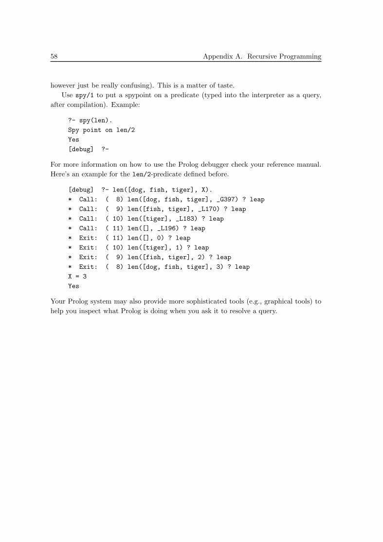
58 Appendix A. Recursive Programming

however just be really confusing). This is a matter of taste.

Use spy/1 to put a spypoint on a predicate (typed into the interpreter as a query,

after compilation). Example:

?- spy(len).

Spy point on len/2

Yes

[debug] ?-

For more information on how to use the Prolog debugger check your reference manual.

Here’s an example for the len/2-predicate defined before.

[debug] ?- len([dog, fish, tiger], X).

* Call: ( 8) len([dog, fish, tiger], _G397) ? leap

* Call: ( 9) len([fish, tiger], _L170) ? leap

* Call: ( 10) len([tiger], _L183) ? leap

* Call: ( 11) len([], _L196) ? leap

* Exit: ( 11) len([], 0) ? leap

* Exit: ( 10) len([tiger], 1) ? leap

* Exit: ( 9) len([fish, tiger], 2) ? leap

* Exit: ( 8) len([dog, fish, tiger], 3) ? leap

X = 3

Yes

Your Prolog system may also provide more sophisticated tools (e.g., graphical tools) to

help you inspect what Prolog is doing when you ask it to resolve a query.

Index

Symbols=/2 . . . . . . . . . . . . . . . . . . . . . . . . . . . . . . . . . . . . . 7

\=/2 . . . . . . . . . . . . . . . . . . . . . . . . . . . . . . . . . . . 13

\+-Operator . . . . . . . . . . . . . . . . . . . . . . . . . . . .42

Aanonymous variable . . . . . . . . . . . . . . . . . . . . . 5

append/3 . . . . . . . . . . . . . . . . . . . . . . . . . . . . . . 18

arithmetic evaluation. . . . . . . . . . . . . . . . . . .21

associativity. . . . . . . . . . . . . . . . . . . . . . . . . . . .28

associativity patterns . . . . . . . . . . . . . . . 28, 29

atom . . . . . . . . . . . . . . . . . . . . . . . . . . . . . . . . 5, 49

atom/1 . . . . . . . . . . . . . . . . . . . . . . . . . . . . . . . . . . 7

Bbacktracking . . . . . . . . . . . . . . . . . . . . . . . 10, 35

problems with . . . . . . . . . . . . . . . . . . . . . 36

bar notation . . . . . . . . . . . . . . . . . . . . . . . . . . . 15

body of a rule . . . . . . . . . . . . . . . . . . . . . . . . . . . 6

built-in predicate

=/2 . . . . . . . . . . . . . . . . . . . . . . . . . . . . . . . . . 7

\=/2 . . . . . . . . . . . . . . . . . . . . . . . . . . . . . . . 13

\+/1 . . . . . . . . . . . . . . . . . . . . . . . . . . . . . . . 42

append/3 . . . . . . . . . . . . . . . . . . . . . . . . . . 18

atom/1 . . . . . . . . . . . . . . . . . . . . . . . . . . . . . .7

call/1 . . . . . . . . . . . . . . . . . . . . . . . . . . . . 45

compound/1 . . . . . . . . . . . . . . . . . . . . . . . . . 7

consult/1 . . . . . . . . . . . . . . . . . . . . . . . . . . 7

current_op/2 . . . . . . . . . . . . . . . . . . . . . 28

fail/0 . . . . . . . . . . . . . . . . . . . . . . . . . . . . . .7

false/0 . . . . . . . . . . . . . . . . . . . . . . . . . . . . 7

help/1 . . . . . . . . . . . . . . . . . . . . . . . . . . . . . .8

is/2 . . . . . . . . . . . . . . . . . . . . . . . . . . . . . . . 21

last/2 . . . . . . . . . . . . . . . . . . . . . . . . . . . . 18

length/2 . . . . . . . . . . . . . . . . . . . . . . . . . . 18

member/2 . . . . . . . . . . . . . . . . . . . . . . . . . . 18

nl/0 . . . . . . . . . . . . . . . . . . . . . . . . . . . . . . . . 7

op/3 . . . . . . . . . . . . . . . . . . . . . . . . . . . . . . . 30

reverse/2 . . . . . . . . . . . . . . . . . . . . . . . . . 18

select/3 . . . . . . . . . . . . . . . . . . . . . . . . . . 18

spy/1 . . . . . . . . . . . . . . . . . . . . . . . . . . . . . .58

true/0 . . . . . . . . . . . . . . . . . . . . . . . . . . . . . .7

write/1 . . . . . . . . . . . . . . . . . . . . . . . . . . . . 7

Ccall/1 . . . . . . . . . . . . . . . . . . . . . . . . . . . . . . . . .45

clause . . . . . . . . . . . . . . . . . . . . . . . . . . . . . . . . . . . 5

closed world assumption. . . . . . . . . . . . . . . .42

comments . . . . . . . . . . . . . . . . . . . . . . . . . . . . . . 11

compilation. . . . . . . . . . . . . . . . . . . . . . . . . .7, 31

complete induction . . . . . . . . . . . . . . . . . . . . . 55

compound/1 . . . . . . . . . . . . . . . . . . . . . . . . . . . . . 7

compound term . . . . . . . . . . . . . . . . . . . . . . . . . 5

concatenation of lists . . . . . . . . . . . . . . . . . . . 16

conjunction (,). . . . . . . . . . . . . . . . . . . . . . . . .43

consult/1 . . . . . . . . . . . . . . . . . . . . . . . . . . . . . . 7

current_op/2 . . . . . . . . . . . . . . . . . . . . . . . . . 28

cut. . . . . . . . . . . . . . . . . . . . . . . . . . . . . . . . . . . . .38

problems with . . . . . . . . . . . . . . . . . . . . . 40

Ddebugging . . . . . . . . . . . . . . . . . . . . . . . . . . . . . . 57

disjunction (;) . . . . . . . . . . . . . . . . . . . . . . . . . 43

Eempty list . . . . . . . . . . . . . . . . . . . . . . . . . . . . . . 15

Ffact. . . . . . . . . . . . . . . . . . . . . . . . . . . . . . . . . .6, 51

fail/0 . . . . . . . . . . . . . . . . . . . . . . . . . . . . . . . . . . 7

false/0 . . . . . . . . . . . . . . . . . . . . . . . . . . . . . . . . .7

59

60 Index

functor . . . . . . . . . . . . . . . . . . . . . . . . . . . . . . 5, 49

Ggoal execution . . . . . . . . . . . . . . . . . . . . . . 10, 52

ground term. . . . . . . . . . . . . . . . . . . . . . . . . . . . .5

Hhead of a list . . . . . . . . . . . . . . . . . . . . . . . . . . . 15

head of a rule . . . . . . . . . . . . . . . . . . . . . . . . . . . 6

head/tail-pattern. . . . . . . . . . . . . . . . . . . . . . .16

help/1 . . . . . . . . . . . . . . . . . . . . . . . . . . . . . . . . . . 8

Horn formula . . . . . . . . . . . . . . . . . . . . . . . . . . 51

Iinduction . . . . . . . . . . . . . . . . . . . . . . . . . . . . . . 55

infix operator . . . . . . . . . . . . . . . . . . . . . . . . . . 28

is-operator . . . . . . . . . . . . . . . . . . . . . . . . . . . . 21

Llast/2 . . . . . . . . . . . . . . . . . . . . . . . . . . . . . . . . .18

length/2 . . . . . . . . . . . . . . . . . . . . . . . . . . . . . . 18

list . . . . . . . . . . . . . . . . . . . . . . . . . . . . . . . . . . . . . 15

empty . . . . . . . . . . . . . . . . . . . . . . . . . . . . . 15

list notation

bar . . . . . . . . . . . . . . . . . . . . . . . . . . . . . . . . 15

head/tail-pattern . . . . . . . . . . . . . . . . . . 16

internal . . . . . . . . . . . . . . . . . . . . . . . . . . . . 15

literature . . . . . . . . . . . . . . . . . . . . . . . . . . . . . . . . 1

Mmatching . . . . . . . . . . . . . . . . . . . . . . . . 8, 21, 52

operators . . . . . . . . . . . . . . . . . . . . . . . . . . 31

member/2 . . . . . . . . . . . . . . . . . . . . . . . . . . . . . . 18

Nnegation as failure. . . . . . . . . . . . . . . . . . . . . .42

nl/0 . . . . . . . . . . . . . . . . . . . . . . . . . . . . . . . . . . . . 7

number . . . . . . . . . . . . . . . . . . . . . . . . . . . . . . . . . 5

Ooccurs check . . . . . . . . . . . . . . . . . . . . . . . . . . . 53

op/3 . . . . . . . . . . . . . . . . . . . . . . . . . . . . . . . . . . . 30

operator

infix . . . . . . . . . . . . . . . . . . . . . . . . . . . . . . . 28

postfix . . . . . . . . . . . . . . . . . . . . . . . . . . . . . 28

prefix . . . . . . . . . . . . . . . . . . . . . . . . . . . . . . 28

operator definition . . . . . . . . . . . . . . . . . . . . . 30

Pparent goal . . . . . . . . . . . . . . . . . . . . . . . . . . . . .38

postfix operator . . . . . . . . . . . . . . . . . . . . . . . . 28

precedence . . . . . . . . . . . . . . . . . . . . . . . . . . . . . 27

predicate . . . . . . . . . . . . . . . . . . . . . . . . . . . . 5, 49

prefix operator . . . . . . . . . . . . . . . . . . . . . . . . . 28

program. . . . . . . . . . . . . . . . . . . . . . . . . . . . . . . . .6

Qquery . . . . . . . . . . . . . . . . . . . . . . . . . . . . . . . . 6, 51

Rrecursive programming . . . . . . . . . . . . . . . . . 56

resolution . . . . . . . . . . . . . . . . . . . . . . . . . . . . . . 52

reverse/2 . . . . . . . . . . . . . . . . . . . . . . . . . . . . . 18

rule . . . . . . . . . . . . . . . . . . . . . . . . . . . . . . . . . 6, 51

Sselect/3 . . . . . . . . . . . . . . . . . . . . . . . . . . . . . . 18

spy/1 . . . . . . . . . . . . . . . . . . . . . . . . . . . . . . . . . . 58

Ttail of a list . . . . . . . . . . . . . . . . . . . . . . . . . . . . 15

term. . . . . . . . . . . . . . . . . . . . . . . . . . . . . . . . .4, 49

compound . . . . . . . . . . . . . . . . . . . . . . . . . . 5

ground . . . . . . . . . . . . . . . . . . . . . . . . . . . . . . 5

transitive closure . . . . . . . . . . . . . . . . . . . . . . . . 2

translation . . . . . . . . . . . . . . . . . . . . . . . . . . . . . 49

true/0 . . . . . . . . . . . . . . . . . . . . . . . . . . . . . . . . . . 7

Uunification . . . . . . . . . . . . . . . . . . . . . . . . . . . . . 52

Vvariable . . . . . . . . . . . . . . . . . . . . . . . . . . . . . 5, 49

anonymous. . . . . . . . . . . . . . . . . . . . . . . . . .5

Wwrite/1 . . . . . . . . . . . . . . . . . . . . . . . . . . . . . . . . .7

Documents

Introduction to Prolog Programming - NTUAglotta.ntua.gr/courses/Technoglossia/Logic/prolog.pdf · And Introduction to Prolog Programming 3 of bigger. Animal X is bigger than animal