Embed Size (px)
Citation preview
INTRODUCTION 'TOPROBABILITY AND
STATISTICS

INTRODUCTION TO
PROBABILITY ANDSTATISTICS
FROM A BAYESIAN VIEWPOINT
PART 2
INFERENCE
BY
D. V. LINDLEYHead of the Department of Statistics
University College London
CAMBRIDGEAT THE UNIVERSITY PRESS
1970

CAMBRIDGE UNIVERSITY PRESSCambridge, New York, Melbourne, Madrid, Cape Town, Singapore, Sao Paulo, Delhi
Cambridge University PressThe Edinburgh Building, Cambridge C132 8RU, UK
Published in the United States of America by Cambridge University Press, New York
www.cambridge.orgInformation on this title: www.cambridge.org/9780521055635
© Cambridge University Press 1965
This publication is in copyright. Subject to statutory exceptionand to the provisions of relevant collective licensing agreements,no reproduction of any part may take place without the written
permission of Cambridge University Press.
First published 1965Reprinted 1970
Re-issued in this digitally printed version 2008
A catalogue record for this publication is available from the British Library
ISBN 978-0-521-05563-5 hardback
ISBN 978-0-521-29866-7 paperback
To
M. P. MESHENBERG
in gratitude


CONTENTS
Preface page ix
5 Inferences for normal distributions
5.1 Bayes's theorem and the normal distribution 1
5.2 Vague prior knowledge and interval estimatesfor the normal mean 13
5.3 Interval estimates for the normal variance 26
5.4 Interval estimates for the normal mean andvariance 36
5.5 Sufficiency 46
5.6 Significance tests and the likelihood principle 58
Exercises 71
6 Inferences for several normal distributions
6.1 Comparison of two means 76
6.2 Comparison of two variances 86
6.3 General comparison of two means 91
6.4 Comparison of several means 95
6.5 Analysis of variance: between and withinsamples 104
6.6 Combination of observations 112
Exercises 122
7 Approximate methods
7.1 The method of maximum likelihood 128
7.2 Random sequences of trials 141
7.3 The Poisson distribution 153
7.4 Goodness-of-fit tests 157
viii CONTENTS
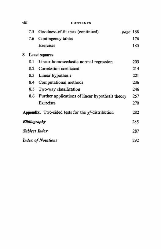
7.5 Goodness-of-fit tests (continued) page 168
7.6 Contingency tables 176
Exercises 185
8 Least squares
8.1 Linear homoscedastic normal regression 203
8.2 Correlation coefficient 214
8.3 Linear hypothesis 221
8.4 Computational methods 236
8.5 Two-way classification 246
8.6 Further applications of linear hypothesis theo ry 257
Exercises 270
Appendix. Two-sided tests for the X2-distribution 282
Bibliography 285
Subject Index 287
Index of Notations 292
ix
PREFACE
The content of the two parts of this book is the minimum that,in my view, any mathematician ought to know about randomphenomena-probability and statistics. The first part deals withprobability, the deductive aspect of randomness. The secondpart is devoted to statistics, the inferential side of our subject.
The book is intended for students of mathematics at a univer-sity. The mathematical prerequisite is a sound knowledge ofcalculus, plus familiarity with the algebra of vectors andmatrices. The temptation to assume a knowledge of measuretheory and general integration has been resisted and, forexample, the concept of a Borel field is not used. The treatmentwould have been better had these ideas been used, but againstthis, the number of students able to study random phenomenaby means of the book would have been substantially reduced.In any case the intent is only to provide an introduction to thesubject, and at that level the measure theory concepts do notappreciably assist the understanding. A statistical specialistshould, of course, continue his study further; but only, in myview, at a postgraduate level with the prerequisite of an honoursdegree in pure mathematics, when he will necessarily know theappropriate measure theory.
A similar approach has been adopted in the level of theproofs offered. Where a rigorous proof is available at this level,I have tried to give it. Otherwise the proof has been omitted(for example, the convergence theorem for characteristic func-tions) or a proof that omits certain points of refinement has beengiven, with a clear indication of the presence of gaps (forexample, the limiting properties of maximum likelihood).Probability and statistics are branches of applied mathematics-in the proper sense of that term, and not in the narrow meaningthat is common, where it means only applications to physics.This being so, some slight indulgence in the nature of the rigouris perhaps permissible. The applied nature of the subject meansthat the student using this book needs to supplement it with
R PREFACE
some experience of practical data handling. No attempt hasbeen made to provide such experience in the present book,because it would have made the book too large, and in any caseother books that do provide it are readily available. The studentshould be trained in the use of various computers and be givenexercises in the handling of data. In this way he will obtain thenecessary understanding of the practical stimuli that have led tothe mathematics, and the use of the mathematical results inunderstanding the numerical data. These two aspects of thesubject, the mathematical and the practical, are complementary,and both are necessary for a full understanding of our subject.The fact that only one aspect is fully discussed here ought not tolead to neglect of the other.
The book is divided into eight chapters, and each chapter intosix sections. Equations and theorems are numbered in thedecimal notation : thus equation 3.5.1 refers to equation 1 ofsection 5 of chapter 3. Within § 3.5 it would be referred to simplyas equation (1). Each section begins with a formal list ofdefinitions, with statements and proofs of theorems. This isfollowed by discussion of these, examples and other illustrativematerial. In the discussion an attempt has been made to gobeyond the usual limits of a formal treatise and to place the ideasin their proper contexts; and to emphasize ideas that are of wideuse as distinct from those of only immediate value. At the endof each chapter there is a large set of exercises, some of whichare easy, but many of which are difficult. Most of these havebeen taken from examination papers, and I am grateful forpermission from the Universities of London, Cambridge, Aber-deen, Wales, Manchester and Leicester to use the questions inthis way. (In order to fit into the Bayesian framework someminor alterations of language have had to be made in thesequestions. But otherwise they have been left as originally set.)
The second part of the book, the last four chapters, 5 to 8, isdevoted to statistics or inference. The first three chapters of thefirst part are a necessary prerequisite. Much of this part hasbeen written in draft twice : once in an orthodox way with theuse only of frequency probabilities; once in terms of probabilityas a degree of belief. The former treatment seemed to have so
PREFACE xi
many unsatisfactory features, and to be so difficult to present tostudents because of the mental juggling that is necessary in orderto understand the concepts, that it was abandoned. This is notthe place to criticize in detail the defects of the purely fre-quentist approach. Some comments have been offered in thetext (§ 5.6, for example). Here we merely cite as an example theconcept of a confidence interval in the usual sense. Technicallythe confidence level is the long-run coverage of the true value bythe interval. In practice this is rarely understood, and istypically regarded as a degree of belief. In the approach adoptedhere it is so regarded, both within the formal mathematics, andpractically. We use the adjective Bayesian to describe an ap-proach which is based on repeated uses of Bayes's theorem.
In chapter 5 inference problems for the normal distributionare discussed. The use of Bayes's theorem to modify priorbeliefs into posterior beliefs by means of the data is explained,and the important idea of vague prior knowledge discussed.These ideas are extended in chapter 6 to several normal distribu-tions leading as far as elementary analysis of variance. Inchapter 7 inferences for other distributions besides the normalare discussed: in particular goodness-of-fit tests and maximumlikelihood ideas are introduced. Chapter 8 deals with leastsquares, particularly with tests and estimation for linear hypo-theses. The intention has been to provide a sound basis con-sisting of the most important inferential concepts. On this basisa student should be able to apply these ideas to more specialisedtopics in statistics : for example, analysis of more complicatedexperimental designs and sampling schemes.
The main difficulty in adopting, in a text-book, a new ap-proach to a subject (as the Bayesian is currently new to statistics)lies in adapting the new ideas to current practice. For example,hypothesis testing looms large in standard statistical practice,yet scarcely appears as such in the Bayesian literature. Anunbiased estimate is hardly needed in connexion with degrees ofbelief. A second difficulty lies in the fact that there is noaccepted Bayesian school. The approach is too recent for themould to have set. (This has the advantage that the student canbe free to think for himself.) What I have done in this book is to
PREFACE
develop a method which uses degrees of belief and Bayes'stheorem, but which includes most of the important orthodoxstatistical ideas within it. My Bayesian friends contend that Ihave gone too far in this : they are probably right. But, to givean example, I have included an account of significance testingwithin the Bayesian framework that agrees excellently, inpractice, with the orthodox formulation. Most of modemstatistics is perfectly sound in practice; it is done for the wrongreason. Intuition has saved the statistician from error. My con-tention is that the Bayesian method justifies what he has beendoing and develops new methods that the orthodox approachlacks. The current shift in emphasis from significance testing tointerval estimation within orthodox statistics makes sense to aBayesian because the interval provides a better description ofthe posterior distribution.
In interpreting classical ideas in the Bayesian framework Ihave used the classical terminology. Thus I have used thephrase confidence interval for an interval of the posterior distri-bution. The first time it is introduced it is called a Bayesianconfidence interval, but later the first adjective is dropped. Ihope this will not cause trouble. I could have used anotherterm, such as posterior interval, but the original term is appo-site and, in almost all applications, the two intervals, Bayesianand orthodox, agree, either exactly or to a good approximation.It therefore seemed foolish to introduce a second term forsomething which, in practice, is scarcely distinguishable from theoriginal.
There is nothing on decision theory, apart from a briefexplanation of what it is in § 5.6. My task has been merely todiscuss the way in which data influence beliefs, in the form of theposterior distribution, and not to explain how the beliefs can beused in decision making. One has to stop somewhere. But it isundoubtedly true that the main flowering of the Bayesianmethod over the next few years will be in decision theory. Theideas in this book should be useful in this development, and, inany case, the same experimental results are typically used inmany different decision-making situations so that the posteriordistribution is a common element to them all.
PREFACE
I am extremely grateful to J. W. Pratt, H. V. Roberts, M.Stone, D. J. Bartholomew; and particularly to D. R. Cox andA. M. Walker who made valuable comments on an early versionof the manuscript and to D. A. East who gave substantiallyof his time at various stages and generously helped with theproof-reading. Mrs M. V. Bloor and Miss C. A. Davies madelife easier by their efficient and accurate typing. I am mostgrateful to the University Press for the excellence of theirprinting.
D.V.L.AberystwythApril 1964

5
INFERENCES FOR NORMALDISTRIBUTIONS
In this chapter we begin the discussion of the topic that willoccupy the rest of the book: the problem of inference, or howdegrees of belief are altered by data. We start with the situationwhere the random variables that form the data have normaldistributions. The reader may like to re-read § 1.6, excluding thepart that deals with the justification of the axioms, beforestarting the present chapter.
5.1. Bayes's theorem and the normal distributionA random sample of size n from a distribution is defined as
a set of n independent random variables each of which has thisdistribution (cf. §§ 1.3, 3.3). If for each real number, 0, belongingto a set (say, the set of positive numbers or the set of all realnumbers), f(x 10) is the density of a random variable, then 0 iscalled a parameter of the family of distributions defined by thedensities (f(x10} (cf. the parameter, p, of the binomial distribu-tion, §2.1). We consider taking a random sample from adistribution with density f(x 10) where 0 is fixed but unknownand the function f is known. Let H denote our state of know-ledge before the sample is taken. Then 0 will have a distributiondependent on H; this will be a distribution of probability in thesense of degree of belief, and we denote its density by rr(B I H).As far as possible 7r will be used for a density of beliefs, p will beused for a density in the frequency sense, the sense that has beenused in applications in chapters 2-4. If the random sample isx = (x1i x2, ..., xn) then the density of it will be, because thexi are independent,
n f(xiI0) = p(xl B, H), say. (1)i.=1
(The symbol H should strictly also appear after 0 on the left-hand side.) The density of beliefs about 0 will be changed by
I LSII
2 INFERENCES FOR NORMAL DISTRIBUTIONS [5.1
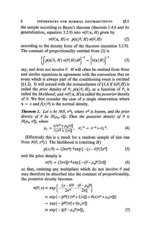
the sample according to Bayes's theorem (theorem 1.4.6 and itsgeneralization, equation 3.2.9) into ir(O I x, H) given by
ir(O x, H) oc p(x B, H) ir(O I H) (2)
according to the density form of the theorem (equation 3.2.9).The constant of proportionality omitted from (2) is
{fxi 0, H) 7r(° I H) de}-1 = (3)
say, and does not involve 0. H will often be omitted from theseand similar equations in agreement with the convention that anevent which is always part of the conditioning event is omitted(§ 1.2). It will accord with the nomenclature of § 1.6 if 7r(0 1 H) iscalled the prior density of 0; p(x 10, H), as a function of 0, iscalled the likelihood; and nr(0 I x, H) is called the posterior densityof 0. We first consider the case of a single observation wherex = x and f(x 6) is the normal density.
Theorem 1. Let x be N(0, o-2), where o.2 is known, and the priordensity of 0 be N(0, Then the posterior density of 0 isN(u1, where
1 - 1 /0.2 -'- 1 /0'22 - 0 -2 + Qp 2 (4)
(Effectively this is a result for a random sample of size onefrom N(0, 0.2).) The likelihood is (omitting H)
p(x 6) = exp [ - (x - 0)2/20.2] (5)
and the prior density is
7r(B) = (27ro'02)-I eXp [ - (B -fto)2/20'0] (6)
so that, omitting any multipliers which do not involve 0 andmay therefore be absorbed into the constant of proportionality,the posterior density becomes
7r(O I x) oc exp { - (X-61)2 - (e-0)220 2o-02
oc exp{-- 62(l/0.2+1/o )+6(x/0'2+ to/0-0))
= exp { - 462/0.1 +
oc exp { - j(O - lul)2/q }, (7)
5.1] BAYES'S THEOREM 3
where, in the first and third stages of the argument, terms notinvolving 0 have been respectively omitted and introduced. Themissing constant of proportionality can easily be found fromthe requirement that 71(0 x) must be a density and thereforeintegrate to one. It is obviously and so the theorem isproved. (Notice that it is really not necessary to consider theconstant at all: it must be such that the integral of 7r(O I x) = 1,and a constant times (7) is a normal distribution.)Corollary. Let x = (x,_, x2, ..., xn) be a random sample ofsize n from N(0, 0-2), where 0.2 is known and the prior densityof 0 is N(,uo, Then the posterior density of 0 is N(un, o n),where nx0.2+ 0.2
An = + /0.0 0n2 = no--2+o-0, (8)n/0-2
and x = n-1 x1.i=1
The likelihood is (equation (1))[_ ]p n x e 2 20'2X B 27x0-2 n/2ex
cc exp [ ex(n/cr2)]
oc exp [ - 4(x - 6)2 (n/cr2)], (9)
where again terms not involving 0 have been omitted and thenintroduced. Equation (9) is the same as (5) with x for x and
for 0.2, apart from a constant. Hence the corollary followssince (8) is the same as (4), again with x for x and for 0-2.
Random samplingWe have mentioned random samples before (§§1.3, 3.3).
They usually arise in one of two situations: either samples arebeing taken from a large (or infinite) population or repetitionsare being made of a measurement of an unknown quantity. Inthe former situation, if the members of the sample are all drawnaccording to the rule that each member of the population hasthe same chance of being in the sample as any other, and thepresence of one member in the sample does not affect the chanceof any other member being in the sample, then the randomvariables, xi, corresponding to each sample member will have
I-2
4 INFERENCES FOR NORMAL DISTRIBUTIONS [5.1
a common distribution and be independent, the two conditionsfor a random sample. t In the second situation the repetitionsare made under similar circumstances and one measurementdoes not influence any other, again ensuring that the two condi-tions for a random sample are satisfied. The purpose of therepetition in the two cases is the same: to increase one's know-ledge, in the first case of the population and in the second caseof the unknown quantity-the latter knowledge usually beingexpressed by saying that the random error of the determinationis reduced. In this section we want to see in more detail thanpreviously how the extent of this increase in knowledge can beexpressed quantitatively in a special case. To do so it is neces-sary to express one's knowledge quantitatively; this can be doneusing probability as a degree of belief (§ 1.6). Thus our task is toinvestigate, in a special case, the changes in degrees of belief,due to random sampling. Of course, methods other thanrandom sampling are often used in practice (see, for example,Cochran (1953)) but even with other methods the results forrandom sampling can be applied with modifications and there-fore are basic to any sampling study. Only random samplingwill be discussed in this book.
Likelihood and parametersThe changes in knowledge take place according to Bayes's
theorem, which, in words, says that the posterior probability isproportional to the product of the likelihood and the priorprobability. Before considering the theorem and its con-sequences let us take the three components of the theorem inturn, beginning with the likelihood. The likelihood is equiva-lently the probability density of the random variables formingthe sample and will have the form (1): the product arising fromthe independence and the multiplication law (equation 3.2.10)and each term involving the same density because of the com-mon distribution. Hence, consideration of the likelihoodreduces to consideration of the density of a single member of
t Some writers use the term `random sample from a population' to mean onetaken without replacement (§1.3). In which case our results only apply approxi-mately, though the approximation will be good if the sample is small relative tothe population.
5.1] BAYES'S THEOREM 5
the sample. This density is purely a frequency idea, empiricallyit could be obtained through a histogram (§2.4), but is typicallyunknown to us. Indeed if it were known then there would belittle point in the random sampling: for example, if the measure-ments were made without bias then the mean value of thedistribution would be the quantity being measured, so know-ledge of the density implies knowledge of the quantity. Butwhen we say `unknown', all that is meant is `not completelyknown', we almost always know something about it; forexample that the density increases steadily with the measure-ment up to a maximum and then decreases steadily-it isunimodal-or that the density is small outside a limited range-it being very unlikely that the random variable is outside thisrange. Such knowledge, all part of the `unknown', consists ofdegrees of belief about the structure of the density and will beexpressed through the prior distribution. It would be of greathelp if these beliefs could be expressed as a density of a finitenumber of real variables when the tools developed in the earlierchapters could be used. Otherwise it would be necessary to talkabout densities, representing degrees of belief, of functions,namely frequency densities, for which adequate tools are notavailable. It is therefore usual to suppose that the density of xmay be written in the form f(x 01i 02, ..., 6S) depending on anumber, s, of real values 6i called parameters; where the functionf is known but the parameters are unknown and therefore haveto be described by means of a prior distribution. Since we knowhow to discuss distributions of s real numbers this can be done;for example, by means of their joint density. It is clear that avery wide class of densities can be obtained with a fixed func-tional form and varying parameters; such a class is called afamily and later we shall meet a particularly useful class calledthe exponential family Q5.5). In this section we consider onlythe case of a single parameter, which is restrictive but stillimportant.
Sometimes f is determined by the structure of the problem:for example, suppose that for each member of a randomsample from a population we only observe whether an event Ahas, or has not, happened, and count the number of times it
6 INFERENCES FOR NORMAL DISTRIBUTIONS [5.1
happens, x, say. Then x has a binomial distribution (§2.1) andthe only parameter is 0 = p, the probability of A on a singletrial. Hence the density is known, as binomial, apart from thevalue of an unknown parameter: the knowledge of the para-meter will have to be expressed through a prior distribution. Inother situations such reasons do not exist and we have to appealto other considerations. In the present section the function f issupposed to be the density of a normal distribution with knownvariance, 0-2, say, and unknown mean. These are the two para-meters of the normal distribution (§2.5). The mean has previ-ously been denoted by u but we shall now use 0 to indicate thatit is unknown and reserve ,u to denote the true, but unknown,value of the mean. Notice that this true value stays constantthroughout the random sampling. The assumption of normalitymight be reasonable in those cases where past, similar experiencehas shown that the normal distribution occurs (§3.6). Forexample, suppose that repeated measurements of a quantity arebeing made with an instrument of a type which has been in usefor many years. Experience with the type might be such that itwas known to yield normal distributions and therefore that thesame might be true of this particular instrument. If, in addition,the particular instrument had been extensively used in the past,it may have been found to yield results of known, constantaccuracy (expressed through the variance or standard devia-tion). In these circumstances every set of measurements of asingle quantity with the instrument could be supposed to havea normal distribution of known variance, only the meanchanging with the quantity being measured : if the instrumentwas free from bias, the mean would be the required value of thequantity. Statistically we say that the scientist is estimating themean of a normal distribution.t This situation could easilyoccur in routine measurements carried out in the course ofinspecting the quality of articles coming off a production line.Often the normal distribution with known variance is assumedwith little or no grounds for the normality assumption, simplybecause it is very easy to handle. That is why it is used here forthe first example of quantitative inference.
t Estimation is discussed in §5.2.
5.1] BAYES'S THEOREM 7
Prior distributionThe form of the prior distribution will be discussed in more
detail in the next section. Here we consider only the meaning ofa prior density of 0. We saw, in § 1.6, what a prior probabilitymeant: to say that a hypothesis H has prior probability p meansthat it is considered that a fair bet of H against not-H would beat odds of p to (1-p). We also saw that a density is a functionwhich, when integrated (or summed), gives a probability (§2.2).Hence a prior density means a function which, when integrated,gives the odds at which a fair bet should be made. If 7T(O) is a
r(0)dO is the prior probability that 0 isprior density thenfo
i
positive, and arfair bet that 0 was positive would be at odds of
Io7r(0)dO to
fo nr(0)dO on. In particular, to suppose, as has
been done in the statement of the theorem, that 0 has priordensity N(,uo, moo) means, among other things, that
(i) 0 is believed to be almost certainly within the interval(,uo - 3o-0, fro + 3o-0) and most likely within (No - 20 0, ,uo + 20 0)(compare the discussion of the normal distribution in § 2.5. We arearbitrarily and conventionally interpreting `most likely' to meanthat the odds against lying outside the interval are 19 to 1).
(ii) 0 is just as likely to be near ,uo + Ao- as it is to be near/to - Ao-, for any A, and in particular is equally likely to begreater than ,uo as less than uo.
(iii) Within any interval (,uo - Ao-0, ,uo + Acr0) the central valuesare most probable and the further 0 is from the mean, the lesslikely are values near 0.
Posterior distribution and precisionOften these three reasons are held to be sufficient for assuming
a normal prior density. But an additional reason is the theorem,which shows that, with a normal likelihood, the posterior distri-bution is also normal. The extreme simplicity of the resultmakes it useful in practice, though it should not be used as anexcuse for assuming a normal prior distribution when thatassumption conflicts with the actual beliefs.
8 INFERENCES FOR NORMAL DISTRIBUTIONS [5.1
The posterior distribution is, like the prior distribution, oneof probability as a degree of belief and because of the normalityenables statements like (i)-(iii) above to be made in the light ofthe datum, the single value of x, but with different values of themean and variance. Let us first consider how these are relatedto the corresponding values of the prior density and the likeli-hood; taking the variance first because it is the simpler. Weshall call the inverse of the variance, the precision. The nomen-clature is not standard but is useful and is partly justified by thefact that the larger the variance the greater the spread of thedistribution and the larger the intervals in (i) above and thereforethe smaller the precision. The second equation in (4) thereforereads:
posterior precision equals the datum precision
plus the prior precision (10)
(this, of course, for normal distributions of datum and priorknowledge and a sample of size 1). The datum precision is theinverse of the random error in the terminology of § 3.3. Itfollows therefore that the posterior precision is necessarilygreater than the prior precision and that it can be increasedeither by an increase in the datum precision (that is by a decreasein the variance of the measurement, or the random error) or byan increase in the prior precision. These statements are allquantitative expressions of rather vaguer ideas that we allpossess: their great merit is the numerical form that they assumein the statistician's language. It is part of the statistician's taskto measure precision. Notice again that it is the inverse of thevariance that occurs naturally here, and not the standard devia-tion which is used in statements (i)-(iii) above. This agrees withearlier remarks (§§2.4, 3.3) that the variance is easier to workwith than the more meaningful standard deviation which canalways be obtained by a final square root operation.
The first equation in (4) can also be conveniently written inwords provided the idea of a weighted mean is used. A weightedmean of two values a1 and a2 with weights w1 and w2 is defined as(w1 a1 + w2 a2)/(wl + w2). With equal weights, w1 = w2, this is theordinary arithmetic mean. As w1 increases relative to w2 the
5.11 BAYES'S THEOREM 9
weighted mean moves towards a1. Only the ratio of weights isrelevant and the definition obviously extends to any number ofvalues. In this terminology
the posterior mean equals the weighted mean of the datum value
and the prior mean, weighted with their precisions. (11)
Information about 0 comes from two sources, the datum andthe prior knowledge. Equation (11) says how these should becombined. The more precise the datum the greater is the weightattached to it; the more precise the prior knowledge the greateris the weight attached to it. Again this is a quantitative ex-pression of common ideas.
Small prior precisionWith equations (10) and (11), and the knowledge that the
posterior density is normal, revised statements like (i)-(iii) canbe made withal and o- replacing Ito and o-o. The most importanteffect of the datum is that the intervals in these statements willnecessarily be narrower, since o < o-o; or, expressed differently,the precision will be greater. A most important special case iswhere the prior precision is very low, or o- is very large. In thelimit as o -- co (10) and (11) reduce to saying that the posteriorprecision and mean are equal to the datum precision and value.Furthermore, both posterior and datum distributions arenormal. Consequently there are two results which are quitedistinct but which are often confused :
(a) the datum, x, is normally distributed about a mean ,uwith variance
(b) the parameter, 0, is normally distributed about a mean xwith variance
The first is a statement of frequency probability, the seconda statement of (posterior) beliefs. The first is a distribution of x,the second a distribution of 0. So they are truly different. Butit is very easy to slip from the statement that x lies within threestandard deviations of It (from (a)) to the statement that 0 lieswithin three standard deviations of x (from (b)-cf. (i) above).Scientists (and statisticians) quite often do this and we see that
10 INFERENCES FOR NORMAL DISTRIBUTIONS [5.1
it is quite all right for them to do so provided the prior precisionis low in comparison with the datum precision and they aredealing with normal distributions.
Precision of random samplesThe corollary establishes similar results for a normal random
sample of size n instead of for a single value. It can also usefullybe expressed in words by saying:
a random sample of size n from a normal distribution isequivalent to a single value, equal to the mean of thesample, with n times the precision of a single value. (12)
(An important proviso is that normal distributions are assumedthroughout.) The result follows since, as explained in the proofof the corollary, (8) is the same as (4) with x for x and n/o'2for ? 2. The result is related to theorem 3.3.3 that, under thesame circumstances, _92(2) = v2/n, but it goes beyond it becauseit says that the mean, x, is equivalent to the whole of thesample. The earlier result merely made a statement about x,for example that it was a more precise determination than asingle observation; the present result says that, with normaldistributions it is the most precise determination. This equiva-lence between x and the sample may perhaps be most clearlyexpressed by considering two scientists both with a randomsample of n measurements. Scientist 1 uses the procedure of thecorollary. Scientist 2 is careless and only retains the numberand mean of his measurements: he then has a single value x,with mean 0 and variance a2 In (§3.3), and a normal distribution(§3.5), and can use the theorem. The two scientists end up withthe same posterior distribution, provided they had the sameprior distribution, so that scientist 2's discarding of the results,except for their number and their mean, has lost him nothingunder the assumptions stated. One of a statistician's main tasksused to be called the reduction of data, replacing a lot of numbersby a few without losing information, and we see now how thiscan be done in the special case of a normal distribution of knownvariance : n values can be ,replaced by two, n and X. But remem-ber that this does assume normality, a very important proviso.
5.1] BAYES'S THEOREM 11
Notice that the proof of the corollary does not use any of thedistributional theory of §§3.3 and 3.5. It follows a direct andsimple calculation in which everything about the sample, exceptx and n, is absorbed into the irrelevant constant of proportion-ality.
Beliefs about the sampleThe constant is not always irrelevant. The general expression
is given in equation (3). n(xI H), which will now be writtenn(x), can be thought of as the distribution of x obtained as amarginal distribution from the joint distribution of x and 0;the joint distribution being defined by means of the conditionaldistribution of x for fixed 0 and the prior distribution of 0.n(x) can be obtained by evaluating (3), but is most easilyobtained by using the results on the bivariate normal distribu-tion in §3.2. In the notation of that section: if y, for fixed x, isN(a + /3x, 0.2) and x is N(,ul, o-1) then y is N(,u2f o-2) with/22 = a + 18,ul, 0-2 = 0-2+R20-2
. Here, in the notation of thissection, x, for fixed 0, is N(0, v2) and 0 is N(,uo, o-02); consequentlyx is N(,uo, 0-2+0-2). The meaning to be attached to this distribu-tion requires some care. Suppose that, before making theobservation x, and therefore when one's knowledge wasdescribed by H, one had been asked one's beliefs about whatvalue the observation would have. There are two sources ofdoubt present about x; first, the doubt that arises from x havinga distribution even if 0 is known, and secondly the doubt aboutthe value of 0 itself. The former is described by p(x 0) and thelatter by 7r(0). They may be compounded in the usual way, asabove, and yield n (x) = fp(x 0) n(B) dB. To illustrate the mean-ing of IT(x) we may say that if x0 is the median of n(x) then,before experimentation, a bet at evens would be offered thatx would be below x0. It is a degree of belief in the outcome ofthe experiment. Notice that p(x 10) can also be thought of asa degree of belief in the outcome of the experiment, but whenthe parameter is known to have the value 0, as distinct from7r(x) which expresses the belief given H. That p(x10) is botha frequency and belief probability causes no confusion since, asexplained in § 1.6, when both types of statement are possible the
12 INFERENCES FOR NORMAL DISTRIBUTIONS [5.1
two probabilities concerned are equal. For example, if theparameter were known to have the value 0 and x, were themedian of p(x 0), then a bet at evens would be offered thatx would be below x, because, on a frequency basis, x would bebelow x, one half of the time.
Example
In the preparation of an insulating material, measurementsare made of the conductivity using an instrument of knownstandard deviation which we can suppose, by suitable choice ofunits, to be one. Prior knowledge of the production processsuggests that most likely the conductivity will lie between 15and 17 (cf. (i) above) and therefore it seems reasonable to sup-pose a prior distribution of conductivity that, in these unitstis N(16, T); that is, p0 = 16, o-0 = 1. Ten readings are madegiving values 16.11, 17.37, 16.35, 15.16, 18.82, 18.12, 15.82,16.34, 16.64, 15.01, with a mean of 16.57. Hence, in the notationof the corollary, n = 10, o = 1, x = 16.57 and from (8)
10x16.57+4x16=16.4110+4
and 0-102 = 10+4 = 14, o-10 = 11V14 = 0.27.
Hence the posterior distribution is N(16.4l, (0.27)2). On thebasis of this it can be said that the mean conductivity of thematerial most likely lies between 15.87 and 16.95, the mostprobable value being 16.41. We shall see in the next sec-tion the formal language that the statistician uses. Noticethat the prior mean is 16, the sample mean is 16.57, and theposterior mean at 16.41 occupies a position between these twobut nearer the latter than the former because the sample meanhas precision (n/o'2) of 10 and the prior precision (0-6-2) is only 4.The posterior precision, at 14, is of course the sum of the two.If the prior knowledge is very imprecise we could allow o-o totend to infinity and attach no weight to it. The posterior mean isthen the sample mean,16.57, but its precision has decreased to 10.
It is instructive to consider what would have been the result
t Notice that in the notation N(µ, vz), the second argument is the variance(here 1/4) and not the standard deviation (1/2).
5.1] BAYES'S THEOREM 13
had the prior distribution been N(10, 4), with a much lowermean. The corollary can still be used but the sample and theprior knowledge are incompatible: before sampling the meanwas almost certainly less than 11.5 (1u0+3o-0) yet the samplevalues are all above 15. It is therefore absurd to take a weightedmean. The experimenter is in the position of obtaining readingsaround 16 when he had expected readings in the interval (6.64,13.36) (that is ,u0 ± 3{o.2 + o-a}-I, from 7r(x)). Clearly he wouldsay that somewhere a mistake has been made either in the priorassessment, or in obtaining the data, or even in the arithmetic.All probabilities are conditional and these are conditional ona mistake not having been made; this is part of H. One shouldbear such points in mind in making any statistical analysis andnot proceed only by the text-book rules.
Robustness
A general remark, that will apply to all the methods to bedeveloped in the remainder of this book, is that any inference,any statement of beliefs, is conditional not only on the data butalso on the assumptions made about the likelihood. Thus here,the posterior normal distribution depends on the normalityassumptions made about the data. It might, or might not, beaffected if the data had not a normal distribution. We saythat an inference is robust if it is not seriously affected by smallchanges in the assumptions on which it is based. The questionof robustness will not be investigated in this book but it isbelieved that most, if not all, of the inference methods given arereasonably robust.
5.2. Vague prior knowledge and interval estimates for thenormal mean
Theorem 1. A random sample, x = (x1, x2, ..., xn), of size n istaken from N(8, 0'2), where 0-2 is known. Suppose there existpositive constants; a, e, M and c (small values of a and e are ofinterest'), such that in the interval I,, defined by
x-A,o/Vn 5 0 < x+A,o/,fin, (1)t Strictly the constants depend on x but the dependence will not be indicated
in the notation.
14 INFERENCES FOR NORMAL DISTRIBUTIONS [5.2
where 21( - Aa) = a, the prior density of 0 lies between c(1- e)and c(1 + e): and outside Ia it is bounded by Mc. Then the posteriordensity 7r(9 I x) satisfies the inequalities
(1-6) n n(x - 9)
(1+e) ( n )1exp(_n(X-11)(2)(1-e) (1-a) 27u72 20-2 )
inside 1,,, and
0 < n(91 x) < (1-e) - a)Ojn
1 e4" (3)
outside I,,.The likelihood of the sample is given by equation 5.1.9
which, on inserting a convenient constant, is
n 1
( -n(.x - 0)2
p(x 10) = GTO-2)exp {
20-2
Hence by Bayes's theorem (equation 5.1.2), within Ia
Ac(1- e) Gne)nexp j - n(
20`2 )2J 1T (e I x)
Ac(l + e)(29f0n
2)f
exp { -n( 200)2)'and outside I,,
0 < 7T(9 I x) 5 AMc-2)
fexp { -
n(20
9)21
(4)
(5)
where A is a constant equal to H(x)-1, equation 5.1.3. Theright-hand inequality in (4) gives
,7r(9 x) d9 Ac(l + e)Jz«
(-2) exp ( - n( 200)2) d9
= Ac(l+e) f e-II'dt, where t
= Ac(l+e) [(D(Aa)-(D(-)L)] = Ac(1+e)(1-a)
since t(- Aa) = 1- (D(.la). Similarly, the same integral exceedsAc(1-e) (1-a) and, if J., is the outside of I,,,
0 5J
n(O I x) d9 < AMca.Ja
5.2] VAGUE PRIOR KNOWLEDGE
Combining these results we have, sinceJ
7r(O x) dO = 1,
Ac(l -e) (1-a) 5 1 5 Ac [(I +e) (1-a)+Ma],and hence
15
(1 +e) (1 1a)+Ma Ac (1-e) (1(6)Inserting (6) in (4) immediately gives (2); a similar insertion in(5) gives (3) on remarking that the maximum value of theexponential in Ja occurs at the end-points 0 = x ± A 0-/Vn whereit has the value e-I2-.
If e and a are small, so that e -P! is also small, the results saythat the posterior distribution of 0 is approximately N(x, 0-2/n).
Definition. If nr(OI x) is any posterior distribution of 0 afterobserving x and I,6(x) is any interval of 0, depending on x and 8,0 S R < 1, such that
7r(O x) dO = 8, (7)
then If(x) is called a 100/3 % (Bayesian) confidence interval for 0(given x). The words in brackets are usually omitted. If(x) isoften called a (Bayesian) interval estimate of 0. 8 is called the(Bayesian) confidence coefficient, or (Bayesian) confidence level.The definition is not restricted to the case of any particularprior distribution.
Discussion of the theorem
The importance of the theorem lies in the fact that it enablesa good approximation to be made to the posterior distributionwhen sampling from a normal distribution of known variance,without being too precise about the prior distribution. The ideabehind the theorem and its proof can be applied to distributionsother than the normal, and is an important statistical tool.With the normal sample the likelihood function is given, apartfrom a constant of proportionality, by equation 5.1.9. If a con-stant (n/21r0-2)I is inserted it is proportional to
nlI
exp2
(8)(2rr0-2/ p {_n,-,
20-2
16 INFERENCES FOR NORMAL DISTRIBUTIONS [5.2
which, as a function of 0, is a normal density function of meanx and standard deviation o-/Vn. We know from the propertiesof the normal density that (8) decreases rapidly as 0 departsfrom x and so does the indefinite integral of (8) (the normaldistribution function) if j- 0 < x. If 0 had the density givenby (8) we could say that 0 almost certainly lay within threestandard deviations (3cr/4/n) of the mean x (cf. equation 2.5.13and 5.1(i)) : generally we could say that the probability that 0lay within A, standard deviations of x (that is, within Ia) is1- 2(D( - )t) = 1- a, say. But, in fact, 0 has not the posteriordensity given by (8), its density is obtained by multiplying (8) bythe prior density and dividing by an appropriate constant.Nevertheless, in I,,, which is the only part of the range of 0 wherethe likelihood is not very small, the prior density from the theo-rem is itself almost constant. Consequently the true posteriordensity of 0 is, in Ia, almost a constant times (8) : this is equa-tion (4). Now what happens outside I., in Ja ? There the likeli-hood contribution, (8), is very small. Hence unless the priordensity is very large in J. their product, the posterior density,must be very small, apart again from this multiplying constant.So, with the boundedness condition on ir(0) in J,,, we obtain (5).It only remains to determine the multiplying constant to makethe integral one. This is done by evaluating separately the in-tegrals over Ia and J,,. The result is (6). If e, a and Ma are smallAc is almost equal to 1 and the limits in (2) differ but little fromthe density (8), that is N(x, o-2/n). The upper bound given in (3)is also small provided a is small, because then ewill be small.Hence the posterior distribution is approximately N(x, 0-2 /n).
ExampleConsider a numerical example. Suppose A = 1.96, or about
2, so that a = 0.05. The interval IL, then extends two standarddeviations either side of X. Consider the values of 0within this interval: it may be judged that prior to takingthe sample no one value of 0 in Ia was more probable thanany other so that 7!(0) is constant within Ia and we can pute = 0. Consider the values of 0 outside 4: it may be judged
t If 0 > x, the indefinite integral rapidly approaches one.
5.21 VAGUE PRIOR KNOWLEDGE 17
that prior to taking the sample no value of 0 there is more thantwice as probable as any value of 0 in I,,; that is M = 2. Then(2) says that the true density certainly lies between multiples(1-a+ Ma)-1 and (1-a)-1 of the normal density within Ia;that is within multiples (1.05)-1 and (0.95)-1, or within about5 % of the normal density. Thus the posterior probability that0 lies within Ia is within 5 % of 0.95, the value for the normaldensity: this posterior probability is at least 0.90. If Aa isincreased to 3.29 so that a = 0.001 then, again taking M = 2,the true density lies within 0.1 % of the normal density, and theposterior probability that 0 lies within two standard deviationsof x differs by only 0.1 % from 0.95. These statements, with aquite accurate probability interpretation, can be made withouttoo precise assumptions about the prior density.
Interpretation of the prior distributionThe restrictions on the prior density correspond to a certain
amount of vagueness about the value of 0 before sampling.Within the effective range of the likelihood no value of 0 isthought to be substantially more probable than any other andvalues outside this range are not much more probable. This iscertainly not the attitude of someone who has strong prior ideasabout the value of 0, as in the example of § 5.1 where the prior dis-tribution was N(16,1) and o/4/n was 1/.10. In the modificationof this example in which ovo was allowed to tend to infinity, theprior distribution does satisfy, for large moo, the conditions ofthe theorem, and the posterior distribution is N(2, Q.2/n). Thescientists' practice of passing from statement (a) to (b) in §5.1is allowable provided the prior distribution has the degree ofvagueness prescribed by the theorem.
Large samplesThe theorem also has a useful interpretation as a limiting
result. It will surely be true for a wide class of prior distribu-tions that the conditions of the theorem will be satisfied forsufficiently large n. As n increases, the width of the interval la,namely 2A o-/Vn, tends to zero, and therefore the condition that7I(0) be almost constant in Ia becomes less of a restriction. Thisis a particular case of a general result that as the sample size
2 LS 11
18 INFERENCES FOR NORMAL DISTRIBUTIONS [5.2
increases the sample values, the data, influence the posteriordistribution more than the prior distribution. We have alreadyhad one example of this in equation 5.1.10: the datum pre-cision is n/o-2, increasing with n, whilst the prior precisionremains constant at 0-6-2. Indeed we know from the laws oflarge numbers (§3.6) that x converges (weakly and strongly)to ,u, the true value of 8, as n co so that prior informationnecessarily becomes irrelevant: at least with one proviso. Ifnr(8) = 0 for any 0 then no amount of experimentation willmake 7r(8 lx) other than 0 (a direct consequence of Bayes'stheorem). Hence n(8) = 0 represents an extreme pig-headedview that will not be influenced by any evidence. The proviso istherefore that ir(8) + 0, for any possible parameter value. (If8 is, for example, a binomial parameter then only values0 S 0 5 1 are possible.) Notice that, as n -> oo, the posteriordistribution tends to be concentrated around one particularvalue, x, and the variance about this value tends to zero.A distribution which has this form means that one is almostcertain that 0 is very near to x and, in the limit n --> oo, that oneknows the value of 0. This acquisition of complete knowledgein the limit as n --> co is a general feature of Bayesian inferences.
Uniform prior distribution
In subsequent sections we shall often find it convenient to usea particular prior distribution: namely, one with constantdensity for all 0, the uniform distribution (cf. § 3.5). The reasonfor this is that it is a reasonable approximation to a distributionsatisfying the conditions of the theorem, and is particularly easyto handle. It should not be treated too literally as a distributionwhich says that any value of 0 is as likely as any other, but ratheras an approximation to one which satisfies the conditions of thetheorem; namely, that over the effective range of the likelihoodany value of 8 is about as likely as any other, and outside therange no value has much higher probability. If 0 has infiniterange (as with a normal mean) then the uniform distributioncannot be defined in the usual way; there is no 7r(8) = c suchthat r
I
cd8=1.
5.21 VAGUE PRIOR KNOWLEDGE 19
Instead it must be defined as a conditional density: if F is anyset of 0 of finite length, then the distribution, conditional on 0belonging to F, has density ir(0 I F) = m(F)-', where m(F) is thelength of F, so that
rfF 7r(0 I F) d0 = m(F)-1JF dO = 1.
In this way we can talk about the uniform distribution on thereal line. As an illustration of the simplicity obtained using theuniform distribution consider the case of normal sampling (§5.1)with 7r(0) constant. The likelihood is given by equation 5.1.9 andthe posterior density must be the same, apart from the constant ofproportionality, which can include the (constant) prior density.The constant of proportionality is obviously (n/2irv2)I and theposterior distribution is N(x, 0-2/n).
Sample informationThe uniform distribution, representing vagueness, can often
be used even when one's prior distribution is quite precise, fora different reason. Much effort has been devoted by scientistsand statisticians to the task of deriving statements that can bemade on the basis of the sample alone without prior knowledge(see § 5.6 for more details). For example, they have tried toanswer the question, what does a sample have to say about 0?Our approach does not attempt to do this: all we claim to dois to show how a sample can change beliefs about 0. Whatchange it effects will depend not only on the sample but also onthe prior beliefs. Modern work suggests that the question justposed has no answer. The approach adopted in this book wouldsuggest that what the questioner means is, what does a samplesay about 0 when the prior knowledge of 0 is slight; or whenthe scientist is not influenced by strong prior opinions about 0.What, in other words, does the sample have to say about 0when the sample provides the bulk of the information about 0?This can be answered using the theorem and the uniform priordistribution, so that even when one has some appreciable priorknowledge of 0 one may like to express the posterior beliefsabout 0 without reference to them. This has the additional
2-2
20 INFERENCES FOR NORMAL DISTRIBUTIONS [5.2
advantage of making the results meaningful to a wider range ofpeople, namely those with vague prior beliefs, and the resultshave a superficial appearance of more objectivity than if asubjective prior distribution had been used.
Problems with substantial prior information
Although the uniform prior distribution will be used in mostof the book, for the reason that most interest centres on thesituation where we wish to express the contribution of thesample to our knowledge, there are problems wherein the con-tributions from prior knowledge and the likelihood are com-parable. They may sometimes be treated by the methods usedfor small prior knowledge, in the following way. If, in respectof observations x now being considered, the prior knowledgehas been obtained from past observations y, known to theexperimenter, the relevant statement of prior knowledge whendiscussing x will be the posterior distribution with respect to thepast observations y. Three distributions of degrees of belief aretherefore available: (1) before the observations y; (2) after y,but before x; (3) after x and y. Although the original problemmay have involved the passage from (2) to (3), and hence astatement of appreciable prior knowledge due to y, it is possibleto consider instead the passage from (1) to (3), incorporatingboth the observations x and y, and for this the prior knowledgeis weak and may therefore be treated by the methods of thisbook. An example is given in the alternative proof of theorem6.6.1. The method is always applicable if x and y come from thesame exponential family (§5.5) and the distributions (1) to (3)are all members of the conjugate family.
There remain problems in which there is an appreciableamount of prior knowledge but it is not possible to be preciseabout the observations from which it has been obtained. Thesecannot be treated directly by the methods of this book, thoughminor modifications to the methods are usually available. Tosee the form of this modification we must await the developmentof further results. For the moment we merely recall the fact that,accepting the arguments summarized in § 1.6, any state of know-ledge or uncertainty can be expressed numerically and therefore
5.21 VAGUE PRIOR KNOWLEDGE 21
in the form of a probability distribution. The form of this distri-bution can usually be ascertained by asking and answeringquestions like, `Do you think the parameter lies below such andsuch a value T, in the way discussed in §5. 1. If the likelihoodbelongs to the exponential family and the prior distribution soobtained can be adequately- described by a member of thefamily conjugate to this family (§5.5) then again the methodsappropriate to vague knowledge may be used. For we maysuppose that the prior distribution of the conjugate family hasbeen obtained by, possibly imaginary, observations y from thesame exponential family starting from weak prior knowledge.An example is given in example 2 of §6.6 and another is givenin §7.2.
Non-normal distributions
It is possible to generalize Theorem 1 to distributions otherthan the normal. The basic idea of the theorem is that if theprior density is sensibly constant over that range of 0 for whichthe likelihood function is appreciable and not too large over thatrange of 0 for which the likelihood function is small, then theposterior density is approximately equal to the likelihood func-tion (apart from a possible constant). The result thus extends todistributions other than the normal. In extensions, the uniformdistribution will often be used to simplify the analysis. Theprinciple of using it has been called by Savage, the principle ofprecise measurement. (Cf. the discussion as n - oo above.)
The theorem is often held to be important for another reasonbut the argument is not satisfactory. In §3.6 we discussed theCentral Limit Theorem 3.6.1 and saw that, provided 82(x1)exists, z will have, as n increases, an approximately normaldistribution, N(0, o-2/n): or, more exactly, n1(x - 0)/v willhave a distribution which tends to N(0, 1). Consequently ifx = (x1, x2, ..., xn) is a random sample from any distributionwith finite variance, the densityI of x is approximately given by
t More research needs to be carried out on what is meant by `adequately'here. It is usually difficult to describe how the final inference is affected bychanges in the prior distribution.
$ The central limit theorem concerns the distribution function, not the densityfunction: but a density is a function which, when integrated, gives the distribu-
22 INFERENCES FOR NORMAL DISTRIBUTIONS [5.2
(5.1.9) again and hence the posterior density, for any sufficientlylarge random sample, is N(x, o.2/n). But the unsatisfactoryfeature of this reasoning is that the equivalent, for the non-normal sample, of the three lines before (5.1.9) has beenomitted. In other words (5.1.9) is not the likelihood of x, butof x, and hence what is true is that for a sufficiently largerandom sample from any distribution of finite variance g(0 1.5c-)(but not necessarily nr(O I x)) is approximately N(x, 0-2/n). Itmight happen that inferences based on x are substantiallydifferent from inferences based on the whole of the sampleavailable. We saw in the last section that with normal samplesx and n are equivalent to x, but this is not true for samples fromother distributions. Indeed, in § 3.6, it was shown that if thesample is from a Cauchy distribution then x has the same dis-tribution as x1, and is therefore only as good as a single observa-tion. Obviously x contains much more information than justx1, say; though the above reasoning would not be used since theCauchy distribution does not satisfy the conditions for theCentral Limit Theorem. The situation with the Cauchy distribu-tion is extreme. It is probably true that in many situations7r(6 1x) will not differ substantially from n (O I x) and it may notbe worth the extra labour of finding the latter.
Confidence intervals
The definition of confidence interval given above is not madefor mathematical use but for convenience in practical applica-tions. Undoubtedly the proper way to describe an inference isby the relevant distribution of degrees of belief, usually theposterior distribution. But, partly for historical reasons, partlybecause people find the idea of a distribution a little elaborateand hard to understand (compare the use of features of distri-butions in §2.4), inferences have not, in practice, been describedthis way. What is usually required is an answer to a question suchas `in what interval does 0 most likely lie?'. To answer this theconcept of a confidence interval has been introduced. A valuetion function and in this sense the integration of the normal density gives thecorrect approximation. The central limit theorem does not say that the densityof x tends to the normal density, though usually this is true and conditions forit are known.
5.21 VAGUE PRIOR KNOWLEDGE 23
of /3 commonly used is 0.95 and then an interval is quoted suchthat the posterior probability of 0 lying in the interval is 0.95.For example, in the situation of the theorem
(.x -1.96x-/Vn, x + 1.96x'/.Jn)
is an approximate 95 % confidence interval for 0: one would beprepared to bet 19 to 1 against 0 lying outside the interval.A higher value of /3 gives a wider interval and a statement ofhigher probability: /3 = 0.99 is often used, giving (X - 2.58o'/4/n,2+2.58v/Vn) in the normal case. Values of /3 near oneare those most commonly used but there is sometimes anadvantage in using /3 = 0.50 so that 0 is as likely to lie inside theinterval as outside it : indeed this used to be common practice.In the normal case the result is (x - 0.67oiVn, x + 0.67o'/Vn) and0.67x'/4/n is called the probable error of X. Modern practice useso-/Jn and calls it the standard error. Thus the sample mean, plusor minus two standard errors, gives a 95 % confidence intervalfor the normal mean.
An important defect of a confidence interval is that it doesnot say whether any values of 0 within the interval are moreprobable than any others. In the normal case, for example,values at the centre, 0 = x, are about seven times more probablethan values at the ends, 0 = x ± 1.96o'/Jn, in the case of a 95 %interval (0(0) = 0.3989, c(2) = 0.0540 and their ratio is 7.39:for the notation see §2.5). The difficulty is often avoided in thecase of the normal mean by quoting the interval in the formx ± 1.96o'/Vn; thus, in the numerical example of the last sectionwith o- -* oo, the mean conductivity would be described as16.57 ± 0.63. This indicates that the most probable value is16.57, but that values up to a distance 0.63 away are not im-probable. Sometimes the most probable value alone is quotedbut this is bad practice as no idea of the precision (in the senseof the last section) is provided. Such a single value is anexample of a point estimate (as distinct from an interval esti-mate). Point estimates have their place, either in conjunctionwith a standard error, or in decision theory, but will not bediscussed in detail in this book. Their place in most problemswill be taken by sufficient statistics (§5.5).
24 INFERENCES FOR NORMAL DISTRIBUTIONS [5.2
EstimationSomething, however, must be said about estimates and
estimation because the terms are so commonly used in statisticalwriting. Current statistical thinking divides problems of infer-ence rather loosely into problems of estimation and problemsof tests of hypotheses. The latter will be discussed in §5.6. It isdifficult to draw a hard and fast distinction between the twotypes of problem, but a broad dividing line is obtained bysaying that hypothesis testing is concerned with inferences abouta fixed value, or set of values, of 0 (for example, is 0 = 7 areasonable value, or is it reasonable that 6 S 0 S 8) whereasestimation problems have no such fixed value in mind and, forexample, may conclude with a statement that 0 lies between6 and 8 (as with a confidence interval) ; the values 6 and 8having no prior significance. The distinction may be illustratedby inferences appropriate to the two situations:
(a) Is the resistance of a new alloy less than that of aluminium ?(b) What is the resistance of this new alloy?The former demands a statement relative to the resistance of
aluminium: the latter requires no such consideration. We shalldefine significance tests of hypotheses in § 5.6. We shall occa-sionally use the term, `an estimate of a parameter', when we referto a value which seems a fairly likely (often the most likely if itis the maximum likelihood estimate, §7.1) value for the para-meter. As just mentioned such an estimate should have associ-ated with it some idea of its precision. A rigorous definition ofa least-squares estimate is given in § 8.3.
Choice of a confidence intervalConfidence intervals are not unique : there are several
intervals containing an assigned amount of the posteriorprobability. Thus, in the case of the normal mean the infiniteinterval 0 > x -1.64o-lVn is a 95 % confidence interval since1(-1.64) = 0.05. In this book a confidence interval willusually be chosen such that the density is larger at any point inthe interval than it is at any point outside the interval; pointsinside are more probable than points outside. This rules out the
5.21 VAGUE PRIOR KNOWLEDGE 25
infinite interval just quoted since J e- l 70of/, Jn has higherdensity, for example, than x + 1.800/Jn. The reason for thechoice is that the interval should contain the more probablevalues and exclude the improbable ones. It is easy to see thatthis rule gives a unique interval (apart from arbitrariness if thereare values of equal probability). It can also be shown that thelength of the interval so chosen is typically as small as possibleamongst all confidence intervals of prescribed confidence co-efficient. This is intuitively obvious : thinking of a probabilitydensity in terms of the mass density of a rod (§2.2) the part ofthe rod having given mass (confidence coefficient) in the leastlength is obtained by using the heavier parts (maximum density).A rigorous proof can be provided by the reader. Notice thatthe rule of including the more probable values is not invariantif one changes from 0 to some function of 0, 0(0), because in sodoing the density changes by a factor Idc/d0I (theorem 3.5.1) sothat the relative values of the densities at different values of 0(and hence 0) change and a high density in terms of 0 may havea low one in terms of 0. Usually, however, there is some reasonfor using 0 instead of 0. For example, here it would be un-natural to use anything other than 0, the mean.
Several parametersThe idea of a confidence interval can be generalized to a
confidence set. If S,6(x) is any set of values of 0 (not necessarilyan interval) with
rr(O x) dO (9)sS(:)
then Sf(x) is a confidence set, with confidence coefficient /3.The definition of confidence sets enables one to make con-
fidence statements about several parameters, though this is rarelydone. It is only necessary to consider the joint posterior dis-tribution of several parameters and to replace (9) by a multipleintegral.
The definition of confidence interval given here is not the usualone and hence the qualification, Bayesian. The usual one will begiven later (§ 5.6) together with our reasons for altering thedefinition. In most problems the intervals produced according
26 INFERENCES FOR NORMAL DISTRIBUTIONS [5.2
to our definition will be identical with those produced by theusual definition, and from a statistician's practice one wouldnot be able to tell which definition was being used.
5.3. Interval estimates for the normal varianceIn this section, as in the last, the data are a random sample
from a normal distribution but instead of the mean beingunknown it is the variance whose prior and posterior distribu-tions interest us, the mean having a known value. If a randomvariable x, in this context often denoted by x2, has a density
exp {- Zx}xm-1 /2m(m - 1)!
= exp { - Jx2} (x2)1v-1/21"(1v - 1)! (1)
for x > 0, and zero for x < 0, it is said to have a x2-distributionwith v degrees of freedom, where v = 2m > 0.
Theorem 1. Let x = (x1, x2, ... xn) be a random sample of size nfrom N(,u, 0), where p is known, and the prior density of vo v,2,/0 bex2 with vo degrees of freedom; then the posterior density of(vo vo + S2)/0 is x2 with P,, + n = v1, say, degrees of freedom, where
nS2 = E (X #)2.
i=1
If the random variable x = vov02/0 has prior density given by(1) it follows from theorem 3.5.1 that 0 = vovolx has priordensity
expt - vo
Co) vo 2 /2v-(vo -1) !(vo010(_V
oc exp 0o} 0-1vo-1, (2)
since dx vovod0/02.
The likelihood of the sample is
p(x 10) = (2170)-1n exp { - E (xi -,u)2/2B} oc e-S$/200-1n. (3)t i=1
Hence using Bayes's theorem with (2) and (3) as the valuesof prior density and likelihood, the posterior density is pro-portional to a-(vo0-p+52)1288-1(n+vo)-1. (4)
5.31 NORMAL VARIANCE 27
It only remains to note that (2) and (4) are the same expressionswith vo o-o and vo of the former replaced by vo v0 2+S2 andvo + n = v,_ in the latter. Since (2) is obtained from x2, so is (4)and the theorem follows.
We record, for future reference, the following result.
Theorem 2.
f0,0e -A10 0-m dO = (m - 2)! 1A--1 (A > 0, m > 1).
The substitution x = A/B, with dx = -A d0102 gives (§2.3)
Joe xxm-2 dx/Am-1 = (m-2)!/A--l.
ExampleThe situation envisaged in this section where a random
sample is available from a normal distribution of known meanbut unknown variance rarely occurs in practice: but the mainresult (theorem 1) is similar in form to, but simpler than,a more important practical result (theorem 5.4.2) and it mayhelp the understanding to take the simpler result first. It canoccur when a new piece of testing apparatus is being used forthe first time : for example, suppose someone comes along witha new instrument for measuring the conductivity, in the exampleof § 5. 1, which he claims has smaller standard deviation than theinstrument currently in use (of standard deviation unity).A natural thing to do is to measure several times, n say, theconductivity of a piece of material of known conductivity, ,u.If the instrument is known to be free from bias and is assumedto yield a normal distribution, each x= is N(,a, 0) with unknownprecision 0-1: the problem is to make inferences about 0 (orequivalently 9-1). The snag here is the phrase `known to be freefrom bias'. This is rather an unusual situation; normally ,u isalso unknown, methods for dealing with that problem will bediscussed in §5.4.
The x2-distributionThe x2-distribution was known to Helmert in 1876, but its
importance in statistics dates from its introduction in 1900 by
28 INFERENCES FOR NORMAL DISTRIBUTIONS [5.3
Karl Pearson in a problem to be considered later (§7.4). It isnot a complete stranger to us, for suppose y has a P(n, A)-distri-bution (§2.3) and let x = 2Ay; then since dx = 2Ady it followsfrom theorem 3.5.1 that x has the density (1). Hence if y isI(n, A), 2Ay is x2 with 2n degrees of freedom: conversely, if x isx2 with v degrees of freedom then x/2A is P(Zv, A). The reasonsfor using the x2-distribution will appear when we examine state-ment (b) below. Essentially they are that it is a convenientrepresentation of many states of belief about 0 and that it leadsto analytically simple results. There is no obligation to use x2:it is merely convenient to do so. The reason for the name`degrees of freedom' for v will appear later (§6.1).
For v > 2 the density, (1), of the X2-distribution increasesfrom zero at x2 = 0 to a maximum at x2 = v - 2 and thendiminishes, tending to zero as x2 --j oo. For v = 2 the densitydiminishes from a finite, non-zero value at x2 = 0 to zero asx2 -> co. For 0 < v < 2 the density tends to infinity as x2 - 0,to zero as x2 -_> oo and decreases steadily with x2. The mean ofthe distribution is v and the variance 2v. All these resultsfollow from similar properties of the F-distribution (§2.3, andequation 2.4.9). For large v the distribution of x2 is approxi-mately normal. A proof of this is provided by relating x2 to Fand using the facts that the sum of independent F-distributionswith the same parameter has also a P-distribution with indexequal to the sum of the indices (§3.5), and the Central LimitTheorem (3.6.1) (see §3.6).
Prior distributionLet us now consider what it means to say that the prior
density of vo O-010 is x2 with vo degrees of freedom, so that thedensity of 0 (the unknown variance of the normal distribution)is given by (2). In this discussion we omit the suffix 0 forsimplicity. For all v > 0 the latter density increases from0 at 0 = 0 to a maximum at 0 = cr2v/(v + 2) and then tends tozero as 0 - oo. The density has therefore the same general shapefor all degrees of freedom as the X2 -distribution itself has fordegrees of freedom in excess of two. To take it as prior densityfor 0 is equivalent to saying that values that are very large
5.31 NORMAL VARIANCE 29
or very small are improbable, the most probable value iso'2v/(v+2) and, because the decrease from the maximum as 0increases is less than the corresponding decrease as 0 diminishes,the values above the maximum are more probable than thosea similar distance below the maximum. The expectation andvariance of 0 are most easily found by remarking that sincevo2/0 is x2 with v degrees of freedom x = is 17(11 v, 1) withdensity e-xxl1'-1/(2 v - 1)! : hence
1 e-xxl»-2 dx/( v - 1) !9'(0) = Ivo-2/'
= 0-2V/(v - 2) (5)
and 61(02) = *v2v4 f e xxl°-3dx/(iv-1)!
= o4v2/(v - 2) (v - 4),so that _92(o) = (B2) - i 2(B) = 20'4v2/(v - 2)2 (v - 4). (6)
These results are only valid if v > 4, otherwise the variance isundefined (or infinite). If v is large the values are approxi-mately 0-2 and 2o4/v. Hence the two numbers at our disposal,0'2 and v, enable us to alter the mean and variance of the priordistribution: o2 is approximately the mean (and also the mostprobable value) and V(21v) is approximately the coefficient ofvariation. Large values of v correspond to rather precise know-ledge of the value of 0 prior to the experiment. The two quantities,0-2 and v, therefore allow considerable variation in the choice ofprior distribution within this class of densities.
We note, for future reference (§7.1), that the prior distributionof 0, like x2, tends to normality as v oo. To prove this considerz = (0 - o-2)/(2o4/v)l with approximately zero mean and unitstandard deviation. From (2), z has a density whose logarithmis
VG-2
2 - (jv + 1) In (zo 2V(2/v) + (72)2(zv2V (2/v) + )
= -jv(1 +z4/(2/v))-1-(v+ 1)In(1 +zV(2/v))
omitting terms not involving z. Expansion of this in powers ofv-l gives -Zz2 + O(v-l) which proves the result.
30 INFERENCES FOR NORMAL DISTRIBUTIONS [5.3
Simpler results are obtained by considering vrr2/0, theparameter in terms of which the theorem is couched. Fromthe mean and variance of x2 quoted above 6'(vrr2/0) = v and
92(vrr-2/B) = 2v so that g(O-1) = o--2 and _92(e-1) = 2o--4/p.0-1 is what we called the precision in §5.1. The mean precisionis therefore 0-2 (hence the notation) and the coefficient ofvariation of the precision is (now exactly) 4J(2/v).
LikelihoodNext consider the likelihood (equation (3)). The remarkable
thing about this is that it only depends on S2 = (x, -,u)2 and n.
In other words, the scientist can discard all his data providedVonly that he retains the sum of squares about the known meanand the size of the sample. The situation is comparable to thatin § 5.1 where only the mean x and n were needed to provide allthe information about the mean: here S2 and n provide all theinformation about the variance. This is a strong reason forevaluating S2 and not some other statistic (see §2.4) such as
n1x, -,ui in order to estimate the variance: but notice the
i=1result assumes the distribution from which the sample is takento be normal (compare the discussion of x and the Central LimitTheorem in § 5.2).
Posterior distributionThe theorem says that the posterior distribution is of the
same form as the prior distribution but with vorra replaced byvo rro + S2 and vo by vo + n = vl. The interpretation of theposterior distribution is therefore the same as for the priordistribution with these numerical changes. The result is mosteasily understood by introducing the quantity
s2 = S2/n = (xi-1a)2/n.=1
The random variables (xi -,u)2 are independent and identicallydistributed with mean S [(x, -,u)2] = o.2, the true value of thevariance of the sample values. Hence since s2 is a mean of nsuch values it tends to o.2, as n --> oo, by the strong law of large
5.31 NORMAL VARIANCE 31
numbers (theorem 3.6.3). Consequently s2 is an estimate of 0.2from the sample. Now prior to sampling the most probablevalue of 0 was o o vo/(vo + 2) and its mean was of v0/(v0 -2),vo > 2, so that tea, between these two values, to avoid complica-tions with odd 2's, is an estimate of U2 from prior knowledge.The posterior value corresponding to o-02 is (vo o'02 + ns2)/(vo + n),which is a weighted mean of prior knowledge (moo) and sampleknowledge (s2) with weights vo and n. The weights are appro-priate because we saw that large values of vo correspond torather precise knowledge of 0 before the experiment and largevalues of n correspond naturally to a lot of knowledge from thesample. Hence the result for the variance is very similar to thatfor the mean (equation 5.1.8) ; in both cases evidence from thesample is combined with the evidence before sampling, usinga weighted mean. The posterior density of 0 has mean andvariance
-9(0 I x) = (vo o + S2)/(vo + n - 2), (7)
_92(0 X) = 2(voo +S2)2/(VO+n-2)2 (vo+n-4) (8)
from (5) and (6). These expressions are valid providedvo + n - 4 > 0. The approximate results are that the mean is(vo of + ns2)/vl = 0-i, say, and the coefficient of variation isJ(2/v1). The coefficient of variation is thus reduced by sampling,from J(2/vo), corresponding to an increase in our knowledgeof 0 due to sampling. As n ->. oo the variance of 0 tends to zeroand the mean behaves like S2/n = s2, tending to 0-2. So thatwith increasing sample size we eventually gain almost completeknowledge about the true value of 0. Similar results are avail-able in terms of the precision 0-1.
Vague prior information
In the normal mean situation (§5.1) it was explained thatspecial attention is paid to the case where the prior information isvery imprecise: in the notation of that section, 0o -± oo. Also, in§ 5.2, it was shown that a wide class of prior distributions couldlead to results equivalent to large vo and that a convenient priordistribution would be a uniform distribution of the unknownparameter, there the mean. In these circumstances the weighted
32 INFERENCES FOR NORMAL DISTRIBUTIONS [5.3
mean of ,uo and x depends less on ,uo and more on x and in thelimit as oo -->- oo, 0 is N(x, o.2/n). Closely related results apply inthe normal variance situation. Very imprecise prior informationclearly corresponds to vo -- 0; for example, the coefficient ofvariation of 0-1, J(2/vo), -> oc. Then the weighted mean dependsless on the prior value vo and more on s2, and in the limit asvo --> 0 we have the simple result that S2/0 is x2 with n degrees offreedom. We shall not give the equivalent result to theorem5.2.1 for the variance situation, but there exists a wide class ofprior distributions, satisfying conditions similar to those in thattheorem, which leads to this last result as an approximation.A convenient prior distribution is obtained by letting vo -> 0 in(2). That expression may be written, with a slight rearrange-ment, as r
vo °'o yo o. 'vo 1 1exp j - 29 } (20 (ivo -1) ! 0
and (jv0 -1) ! times this tends, as vo -> 0, to 0-1. Hence theprior distribution suggested has density proportional to 0-1.This is not a usual form of density since, like the uniform distri-bution of the mean, it cannot be standardized to integrate toone. But like the uniform distribution it can be treated asa conditional density (§ 5.2). With this prior distribution and thelikelihood given by (3), the posterior distribution is obviously,apart from the constant of proportionality, e-Sh/2ee-In-1, which
is (4) with vo = 0. Hence the usual form of inference made inthe situation of the theorem, that is with imprecise priorknowledge, is
(b) the parameter 0 is such that S2/0 is distributed in a x2-distribution with n degrees of freedom.
This statement should be compared with (5.1(b)) to whichcorresponds a parallel statement (5.1(a)) with, however, quitea different meaning. It is interesting to note that there is asimilar parallel statement corresponding to (b). To obtain thiswe recall a remark made in §3.5 and used above that the sumof two (and therefore of any number) of independent P-variables with the same parameter has also a P-distributionwith that parameter and index equal to the sum of the indices.Also, from example 3.5.1 we know that (X,_#)2 is P(+, 1/2o-2),
5.3] NORMAL VARIANCE 33
so that S2 = E(xi -,u)2 is F(n/2, 112o-1), and hence, by therelationship between the F- and x2-distributions, we have
(a) the datum S2 is such that S2/o-2 is distributed in a x2-distribution with n degrees of freedom. Warnings about con-fusing (a) and (b) similar to those mentioned in §5.1 apply here.
The conditional density 0-1 is related to the uniform distribu-tion over the whole real line in the following way. Let 0 = In 0.Then the density of 0 is constant, since do/d0 = 0-1 (theorem3.5.1) and as ln0 extends from -oo to +oo, the logarithm of thevariance has a uniform distribution over the whole real line.The distribution arises in yet another way. The density of anyx, is (27T0)-I exp { - (xi -,u)2/20}. Effect transformations of xiand 0 as follows: zi = ln[(xi-,u)2], 0 = 1nO. The densityof zi is proportional to ehzi-0)exp{-1 e(zi-0>}, a function ofzi - O only. Similarly, in the case of the normal mean thedensity of xi (without any transformation) is proportional toexp { - - (x, - 0)2}, a function of xi - 0 only. If a random variablex has a density p(x 10), depending on a single parameter 0,which is a function only of x - 0 then 0 is said to be a locationparameter for x (cf. §2.4). It means that as 0 changes thedensity remains unaltered in shape and merely moves along thex-axis. Our remarks show that the normal mean and thenormal log-variance (or equally log-standard deviation) areboth location parameters. It therefore seems in good agreementwith our choice of a uniform distribution of the mean in § 5.2 touse a uniform distribution of log-variance here. Both in thecase of the normal mean and the normal variance, it is becausethe parameter is transformable to one of location that thereexist related pairs of statements (a) and (b). If
p(x 10) = Ax - 0)
an operation on 0 is an operation on x - 0 or equivalently x:thus,
f tf(t - 0) dO = r1 f(u) du = (W w+1 f(x - w) dx
t-1 J O w
so that statements made about 0 (type (b)) correspond tostatements about the datum (type (a)).
3 LSII
34 INFERENCES FOR NORMAL DISTRIBUTIONS [5.3
Confidence intervals
It remains to discuss how confidence interval statements maybe made about 0 on the basis of the posterior distribution. Weshall suppose the posterior distribution to be such that S2/0 isx2 with n degrees of freedom (vo -->0), the case of general vofollows similarly. To make confidence interval statements weneed the distribution function of the x2-distribution for integralvalues of v, the degrees of freedom. This is extensively tabulated;see, for example, Lindley and Miller (1961). To simplify theexposition we introduce some standard terminology. If F(x) isa distribution function, the value xa, supposed unique, such thatF(xa) = 1- a is called the upper 100a Y. point of the distribu-tion: the value xa such that F(xa) = a is called the lower 100apoint. If x is a random variable with F(x) as its distributionfunction p(x < xa) = p(x > xa) = a. The numerical values forthe normal distribution function given in equations 2.5.13 canbe rephrased by saying `the upper 2-1 Y. point of the standard-ized normal distribution is 1.96', etc. Let xa(v) [xa(v)] be theupper [lower] 100a Y. points of the x2-distribution with v degreesof freedom. These are tabulated by Lindley and Miller-[ fora = 0.05, 0.025, 0.01 and 0.005. A confidence interval for 0,with confidence coefficient /j, can then be found from the result
nr(S2/0 > x«(n) l x) = -a = /3,
which gives 7r(6 < S2/xa(n) I x) (9)
on rephrasing the description of the event being considered.Here, in a convention which will be adhered to, /3 = 1- a, a istypically small and /3 near one. This (semi-infinite) interval maybe enough for some practical purposes for it says, with large /3,that one is fairly certain that 0 is less than S21X1 (n). In theexample of conductivity measurements it may be enough toknow that the variance does not exceed that limit: or, equiva-lently, that the precision is greater than x2(n)/S2. However, inmost cases a finite interval is wanted and the usual practice is toobtain it by removing ja from the upper and lower ends of the
t The upper ones only are tabulated for 100a = 10 and 1/10 %.
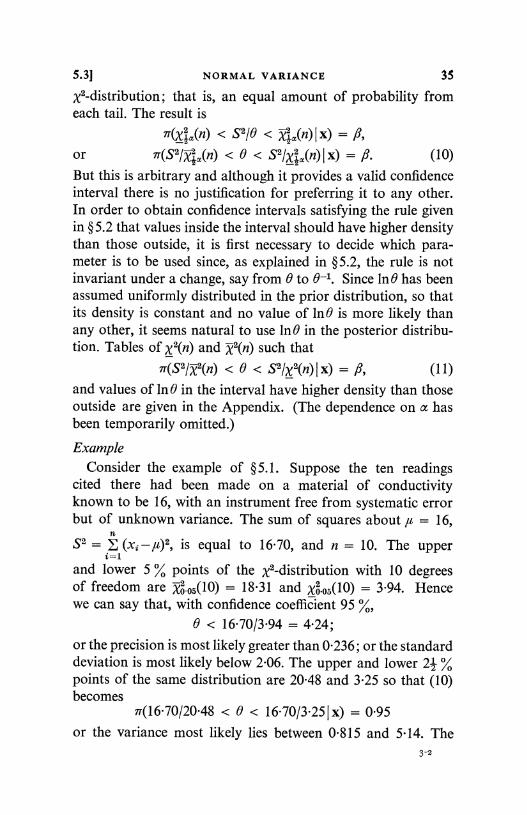
5.3] NORMAL VARIANCE 35
x2-distribution; that is, an equal amount of probability fromeach tail. The result is
n(x2.(n) < S2/0 < te(n) x)or ir(S2/xja(n) < 0 < S2/4Ia(n) I x) = l3 (10)But this is arbitrary and although it provides a valid confidenceinterval there is no justification for preferring it to any other.In order to obtain confidence intervals satisfying the rule givenin § 5.2 that values inside the interval should have higher densitythan those outside, it is first necessary to decide which para-meter is to be used since, as explained in § 5.2, the rule is notinvariant under a change, say from 0 to 0-I. Since In0 has beenassumed uniformly distributed in the prior distribution, so thatits density is constant and no value of ln0 is more likely thanany other, it seems natural to use ln0 in the posterior distribu-tion. Tables of x2(n) and x2(n) such that
1r(S2/)e2(n) < 0 < S2/x2(n) I x)
and values of In 0 in the interval have higher density than thoseoutside are given in the Appendix. (The dependence on a hasbeen temporarily omitted.)
Example
Consider the example of §5.1. Suppose the ten readingscited there had been made on a material of conductivityknown to be 16, with an instrument free from systematic errorbut of unknown variance. The sum of squares about ,u = 16,
nS2 = (x, -,u)2, is equal to 16.70, and n = 10. The upper
and lower 5 % points of the x2-distribution with 10 degreesof freedom are xo.o5(l0) = 18.31 and X02 0.5(10) = 3.94. Hencewe can say that, with confidence coefficient 95 %,
0 < 16.70/3.94 = 4.24;
or the precision is most likely greater than 0.236; or the standarddeviation is most likely below 2.06. The upper and lower 21 %points of the same distribution are 20.48 and 3.25 so that (10)becomes
7r(16.70/20.48 < 0 < 16.70/3.251 x) = 0.95
or the variance most likely lies between 0.815 and 5.14. The3-2
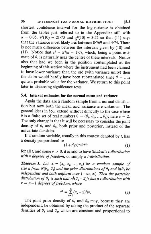
36 INFERENCES FOR NORMAL DISTRIBUTIONS [5.3
shortest confidence interval for the log-variance is obtainedfrom the tables just referred to in the Appendix: still with
0.05, x2(10) = 21.73 and x2(10) = 3.52 so that (11) saysthat the variance most likely lies between 0.769 and 4.74. Thereis not much difference between the intervals given by (10) and(11). Notice that s2 = S2/n = 1.67, which, being a point esti-mate of 0, is naturally near the centre of these intervals. Noticealso that had we been in the position contemplated at thebeginning of this section where the instrument had been claimedto have lower variance than the old (with variance unity) thenthe claim would hardly have been substantiated since 0 = 1 isquite a probable value for the variance. We return to this pointlater in discussing significance tests.
5.4. Interval estimates for the normal mean and varianceAgain the data are a random sample from a normal distribu-
tion but now both the mean and variance are unknown. Thegeneral ideas in § 5.1 extend without difficulty to the case where0 is a finite set of real numbers 0 = (01i 02, ..., 0S); here s = 2.The only change is that it will be necessary to consider the jointdensity of 01 and 02, both prior and posterior, instead of theunivariate densities.
If a random variable, usually in this context denoted by t, hasa density proportional to
(1+t2/v) i(P+1> (1)
for all t, and some v > 0, it is said to have Student's t-distributionwith v degrees of freedom, or simply a t-distribution.
Theorem 1. Let x = (x1, x2i ..., xn) be a random sample ofsize n from N(01, 02) and the prior distributions of 01 and In 02 beindependent and both uniform over (- oo, oo). Then the posteriordistribution of 01 is such that nf(01- x)/s has a t-distribution withv = n -1 degrees of freedom, where
n++
S2 = L (xi - x)2/vi=1
(2)
The joint prior density of 01 and 02 may, because they areindependent, be obtained by taking the product of the separatedensities of 01 and 02, which are constant and proportional to
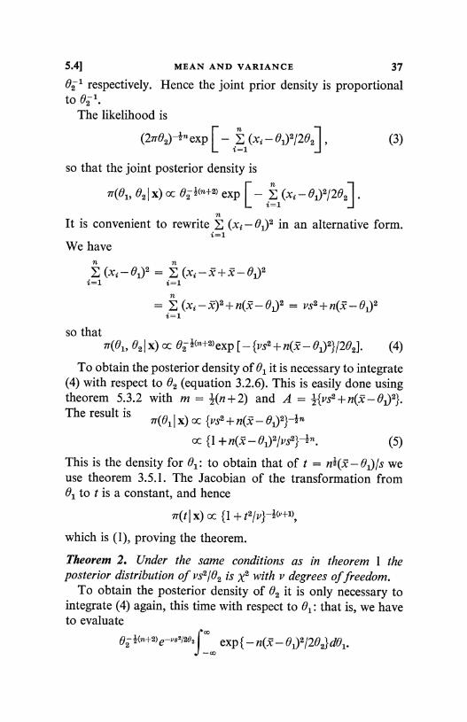
5.4] MEAN AND VARIANCE 37
02-1 respectively. Hence the joint prior density is proportionalto 621
The likelihood is
(27x62)-I n exp C - (xi - 61)2/202] ,i=1
so that the joint posterior density is
(3)
701, 02 I x) cc 62 l(n+2) eXp C - (x. - 61)2/202] .L i=1
It is convenient to rewrite (x1- 61)2 in an alternative form.i=1
We haven n
(xi - 01) 2 = (xi _x + x - 01)2ti=1 i=1
n
(xi - x)2 + n(x - 61)2 = VS2 + n(X - 61)2i=1
so thatn (01, 021 x) cc 02 1(n+2) exp [ - {vs2 + n(x - 01)2}/202j. (4)
To obtain the posterior density of 01 it is necessary to integrate(4) with respect to 02 (equation 3.2.6). This is easily done usingtheorem 5.3.2 with m = 4-(n + 2) and A = {vs2 + n(x- 61)2}.The result is
7T(ol I X) cc {VS2 + n(x - 002}-+ln
cc {l + n(x - 61)2/vS2}-ln. (5)
This is the density for 01: to obtain that of t = nl(x - 01)/s weuse theorem 3.5.1. The Jacobian of the transformation from01 to t is a constant, and hence
7r(t I x) cc {1 + t2/V}-l(v+1),
which is (1), proving the theorem.
Theorem 2. Under the same conditions as in theorem 1 theposterior distribution of vs2/62 is x2 with v degrees of freedom.
To obtain the posterior density of 02 it is only necessary tointegrate (4) again, this time with respect to 01: that is, we haveto evaluate
0 2l (n+2) e-vs2/202j exp {- n(x - 01)2/262} d61.
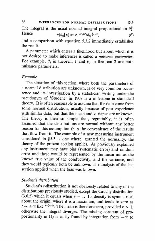
38 INFERENCES FOR NORMAL DISTRIBUTIONS [5.4
The integral is the usual normal integral proportional to 0Q.Hence
77(021 X) cc e-vs2/20202IP-I' (6)and a comparison with equation 5.3.2 immediately establishesthe result.
A parameter which enters a likelihood but about which it isnot desired to make inferences is called a nuisance parameter.For example, 02 in theorem 1 and 0I in theorem 2 are bothnuisance parameters.
Example
The situation of this section, where both the parameters ofa normal distribution are unknown, is of very common occur-rence and its investigation by a statistician writing under thepseudonym of `Student' in 1908 is a milestone in statisticaltheory. It is often reasonable to assume that the data come fromsome normal distribution, usually because of past experiencewith similar data, but that the mean and variance are unknown.The theory is then so simple that, regrettably, it is oftenassumed that the distributions are normal without any betterreason for this assumption than the convenience of the resultsthat flow from it. The example of a new measuring instrumentconsidered in §5.3 is one where, granted the normality, thetheory of the present section applies. As previously explainedany instrument may have bias (systematic error) and randomerror and these would be represented by the mean minus theknown true value of the conductivity, and the variance, andthey would typically both be unknown. The analysis of the lastsection applied when the bias was known.
Student's distribution
Student's t-distribution is not obviously related to any of thedistributions previously studied, except the Cauchy distribution(3.6.5) which it equals when v = 1. Its density is symmetricalabout the origin, where it is a maximum, and tends to zero ast --- ± cc like H°+'). The mean is therefore zero, provided v > 1,otherwise the integral diverges. The missing constant of pro-portionality in (1) is easily found by integration from -oo to
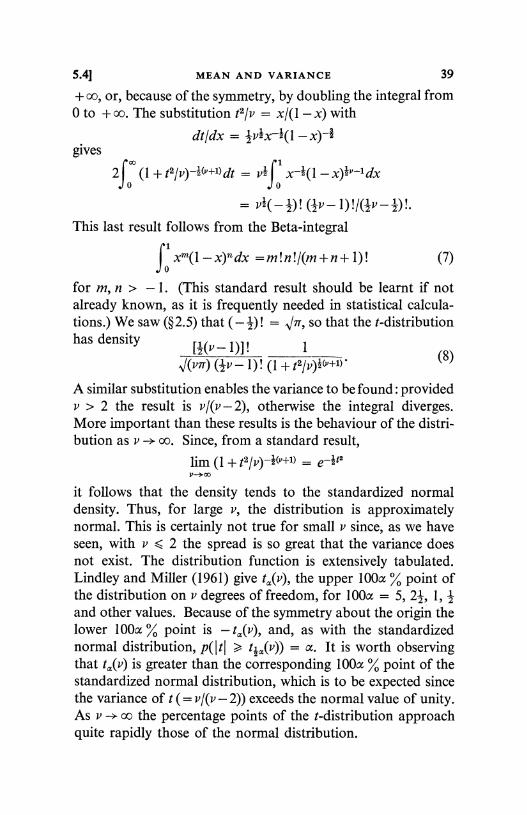
5.4] MEAN AND VARIANCE 39
+ oo, or, because of the symmetry, by doubling the integral from0 to +oo. The substitution t2/v = x/(l - x) with
dt/dx = 4v1x-1(1-x)4gives
2fo (1 + t2/v)- cP+')dt = vIJo
x4(l -x)1i-1dx
= V1( 2)! (2V-1)!I(V-2)!.This last result follows from the Beta-integral
f1xm(l_x)ndx =m!n!/(m+n+ 1)! (7)
for m, n > - 1. (This standard result should be learnt if notalready known, as it is frequently needed in statistical calcula-tions.) We saw (§2.5) that (- 2)! = V7r, so that the t-distributionhas density [(v-1)]! 1
8)4J(v7T) (iv -1) ! (1 + t2/v)1+1). (
A similar substitution enables the variance to be found : providedv > 2 the result is v/(v - 2), otherwise the integral diverges.More important than these results is the behaviour of the distri-bution as v -- oo. Since, from a standard result,
Jim (1 + t2/v)-1(°+u = e-Y2v- -co
it follows that the density tends to the standardized normaldensity. Thus, for large v, the distribution is approximatelynormal. This is certainly not true for small v since, as we haveseen, with v < 2 the spread is so great that the variance doesnot exist. The distribution function is extensively tabulated.Lindley and Miller (1961) give ta(v), the upper 100a % point ofthe distribution on v degrees of freedom, for 100a = 5, 24, 1, zand other values. Because of the symmetry about the origin thelower 100a % point is - ta(v), and, as with the standardizednormal distribution, p(I tj > t1a(v)) = a. It is worth observingthat ta(v) is greater than the corresponding 100a % point of thestandardized normal distribution, which is to be expected sincethe variance of t (= v/(v - 2)) exceeds the normal value of unity.As v -> oo the percentage points of the t-distribution approachquite rapidly those of the normal distribution.
40 INFERENCES FOR NORMAL DISTRIBUTIONS [5.4
Prior distributionSince there are two unknown parameters (that is two para-
meters about which the degrees of belief have to be expressed)it is necessary to consider a joint distribution of them (§3.2). Wehave already discussed at length in the earlier sections of thischapter the prior distribution of either one when the other isknown, 7x(01 102i H), and Ir(e2 101, H). Thus, if 02 = u2 we took7r(81 I (T2, H) to be N(,uo, 01). But we did not say, because we didnot need to, whether ,uo or vo would change with v2. To do thiswe would have to answer the question: if someone came alongand convinced you that the variance of each observation wasnot 0-2, but T2, say, would this change your beliefs about 0,?In many situations it would not and therefore we can take theconditional distribution 701102iH) to be the same for all 02;that is, el and 02 are independent. Similar remarks apply, ofcourse, to 7x(02 1©1, H) provided the precision, 021, is not affectedby the true value 01 being measured. We therefore suppose Bland 02 to be independent, when their joint distribution can bedefined by their separate distributions. In the case of impreciseprior knowledge we saw that it was a reasonable approximationto take 81 and 1n02 to be uniformly distributed over the wholereal line. This explains the choice of prior distribution in thetheorems. These choices are only reasonable in the case of vagueknowledge about independent mean and variance: or, in thespirit of theorem 5.2.1, when the densities of 01 and 1n02 areappreciably constant over the effective range of the likelihoodfunction and not too large elsewhere.
Likelihood
The rearrangement of the likelihood function to obtain (4) isilluminating, besides being necessary for the integration leadingto (6). In the case where only the mean was unknown we saw(§5.1) that the statistician could discard the sample providedthat he retained x and n: when only the variance was unknown(§ 5.3), he needed to retain E(x. -,u)2 and n. Equation (4) showsthat when both mean and variance are unknown and only the
5.4] MEAN AND VARIANCE 41
nnormality is assumed, x, s2 = (xi - x)2/(n - 1) and n need be
2=retained. (Notice that s2 was defined differently in § 5.3, where
nit denoted (xi -,u)2/n.) Again the statistician has achieved
'6=1
a substantial reduction of data (at least for all but very small n)by replacing n numbers by three. The statistics, x and s2 aremost easily calculated by first evaluating Exi and Exi and then
x = Exi/n, s2 = [Exi-(Ex2)2In]/(n-1).
The latter result is easily verified (cf. theorem 2.4.1). x and s2are called the sample mean and sample variance respectively. Ofcourse there is some ambiguity about what should be retained:Exi and Ex?, together with n, would be enough. What isrequired is at least enough for the likelihood to be evaluated:x and s2 are perhaps the most convenient pair of values.
Posterior distribution of the meanNow consider theorem 1. The posterior distribution of 01 is
given by equation (5). The most probable value is x and thedensity falls symmetrically as the difference between 01 and xincreases, the rate of decrease depending mainly on S2. Thesituation is perhaps best understood by passing to t and com-paring the result with that of theorem 5.2.1 where the variancewas known. The posterior distribution of 01 was N(x, o.2/n),
when 01 had constant prior density; and this may be expressedby saying:
(i) If the variance, o.2, is known, nl(01 - x)/o- is N(0, 1).
Compare this with the above theorem which says :
(ii) If the variance is unknown, nl(01- x)/s has a t-distri-bution with v = n -1 degrees of freedom.
The parallelism between (i) and (ii) is obvious: o is replaced by sand the normal by the t-distribution. Since o.2 is unknown inthe second situation it has to be replaced by a statistic ands2 = E(xi - x)2/(n - 1) is a reasonable substitute. We saw in§ 5.3 that E(xi -,u)2/n -_> .2 as n -* oo, but that statistic cannot be
42 INFERENCES FOR NORMAL DISTRIBUTIONS 15.4
used here to replace 0-2 since It is unknown, so E(xq - 2)2/nnaturally suggests itself. In fact
E(X,-X)2 = Y(xi-It)2-n(fc-X)2,
and since x -> It as n -> oo, by the strong law of large numbers,E(x; - x)2/(n - 1) tends to 0.2 as n --> oo. The use of (n - 1) in-stead of n is merely for later convenience (§6.1).
The knowledge contained in the posterior distribution of 01iwhen 02 is unknown, would be expected to be less than when02 was known, since more knowledge is available prior tosampling in the latter case and s has to replace o-. This isreflected in the use of the t-distribution in place of the normal,for we have just seen that it has larger tails than the normalbecause the upper percentage points are higher (compare theuse of the inverse of the variance to measure the precision: herethe precision is (v-2)/v < 1). But as n -> oc, so does v, and thet-distribution approaches the normal. The lack of prior know-ledge about the variance has little effect when the sample sizeis large.
The close relationship between (i) and (ii) enables confidenceinterval statements about 01 to be made in a similar manner tothose in § 5.2. For example, from (i) (X- 1-96o-lVn, X+ 1.96o-/k/n)is a 95 % confidence interval for 01: the corresponding state-ment here is obtained from the t-distribution. We have withQ = 1- a,
p[ - tla(y) < t < t«(y)] = ft
or p[ - tIa(v) < nl(01- JC)/s < t+ia(v)] = R,
giving p[2 - q,,(v) s/Vn < 01 < Jc + q ,,(v) s/Jn] = Q. (9)
With 8 = 0.95 this gives a 95 % confidence interval for 01which has the same structure as the case of known variance,with s for o and t0.025(v) for 1.96. For example, with v = 10,t0.025(10) = 2.23; for v = 20, t0.025(20) = 2.09. Thus if s is nearo, as would be expected, the confidence interval is longer whenthe variance is unknown than when it is known. Intervals like(9), which are symmetric about the origin are obviously theshortest ones and satisfy the rule of § 5.2 because the t-density isunimodal and symmetric about zero.
5.41 MEAN AND VARIANCE 43
Posterior distribution of the varianceThe posterior distribution of 02 in theorem 2 is very similar
to that in §5.3. We put the results together for comparison:(iii) If the mean, u, is known, E(x1-,u)2/02 is x2 with
n degrees of freedom (theorem 5.3.1 with vo = 0).(iv) If the mean is unknown, E(x1- 5)2/02 is x2 with (n - 1)
degrees of freedom (theorem 2).The effect of lack of knowledge of the mean is to replace ,a by x,a natural substitution, and to reduce the degrees of freedom ofx2 by one. The mean and variance of x2 being v and 2v respec-tively, they are both reduced by lack of knowledge on the meanand the distribution is more concentrated. The effect on the dis-tribution of 02, which is inversely proportional to x2, is just theopposite: the distribution is more dispersed. The mean andvariance of 02 are proportional to v/(v - 2) and 2v2/(v - 2)2 (v - 4)respectively (equations 5.3.5, 5.3.6), values which increase as v de-creases from n ton - 1. This is the effect of the loss of informationabout,u. Confidence interval statements are made as in § 5.3, withthe degrees of freedom reduced by one and the sum of squaresabout the sample mean replacing the sum about the true mean.
ExampleConsider again the numerical example of the conductivity
measurements (§5.1). Suppose the ten readings are from anormal distribution of unknown mean and variance; that is,both the systematic and random errors are unknown. Thevalues of x and s2 are 16.57 and 1.490. Hence a confidenceinterval for 01 with coefficient 95 % is 16.57 ± 2.26 x (1.490/10)1;that is 1657 ± 0.87, which is larger than the interval 16.57 ± 0.63,obtained in § 5.2 when rr = 1. A confidence interval for 02 withcoefficient 95 % is (13.41/20.31 < 0 < 13.41/2.95). This isobtained by inserting the values for x2(9) and x2(9) from theappendix, instead of x2(10) and x2(10) used in § 5.3, and thevalue E(x1- x)2 = 13.41. The result (0.660, 4.55) gives lowerlimits than when the mean is known (0.815, 5.14) because partof the variability of the data can now be ascribed to variation ofthe mean from the known value, u = 16, used in § 5.3.
44 INFERENCES FOR NORMAL DISTRIBUTIONS [5.4
Joint posterior distributionThe two theorems concern the univariate distributions of
mean and variance separately. This is what is required in mostapplications, the other parameter usually being a nuisanceparameter that it is not necessary to consider, but occasionallythe joint distribution is of some interest. It is given by equa-tion (4), but, like most joint distributions, is most easily studiedby considering the conditional distributions. From (4) and (6)
ir(61162, x) = 71(61, 621 x)/7T(021 x)
cc 02I exp [ - n(x - 61)2/262], (10)
that is, N(x, 02/n), in agreement with the result of §5.1. Butsince the variance in (10) is 02/n this distribution depends on 02and we see that, after sampling, 01 and 02 are not independent.The larger 02 is, the greater is the spread of the distribution of01, and the less precise the knowledge of 01. This is sensible sinceeach sample value, x1, has variance 02 and has more scatterabout,u the larger 02 is, and so provides less information about,u. If, for example, 02 doubles in value, it requires twice as manysample values to acquire the same precision (n/02) about It.
From (4) and (5), absorbing into the constant of proportion-ality terms which do not involve 02, we have
n(02I 01, x) = ir(01, 621 x)/x(61 I x)
cc 02I(,,+3) exp [ - {VS2 + n(x - 01)2}/202], (11)
that is, {vs2 + n(x - 01)2}/02 is x2 with v + 1 = n degrees of free-dom. Again this involves 01, as it must since 01 and 02 are notindependent. The numerator of the x2 quantity is least when01 = x so that 02, which is this numerator divided by x2, hasleast mean and spread when 01 = x. If x = 61 then the samplemean has confirmed the value of the mean of the distribution,but otherwise x departs from 01 and this may be due to 02i hencethe uncertainty of 02 increases. Although 01 and 02 are notindependent their covariance is zero. This easily follows from(10), which shows that 'ff(61102i x) = x for all 62, and equation
5.4] MEAN AND VARIANCE 45
3.1.21. We shall see later (§7.1) that in large samples the jointdistribution is normal so that the zero covariance will implyindependence. The explanation is that in large samples theposterior density will only be appreciable in a small regionaround 0 = x, B2 = S2, as may be seen by considering theposterior means and variances of 01 and 02, and within thisregion the dependence of one on the other is not strong.
Tabulation of posterior distributionsIt may be helpful to explain why, in the theorems of this
section and the last, the results have been expressed not asposterior distributions of the parameter concerned but asposterior distributions of related quantities: thus, t instead of 01.The reason is that the final stage of an inference is an expressionin numerical terms of a probability, and this means that thedistribution function involved in the posterior distribution hasto be tabulated and the required probability obtained from thetables; or inversely the value of the distribution obtained fora given probability. It is naturally convenient to have firstly,as few tables as possible, and secondly, tables with as few in-dependent variables as possible. In inferences with normalsamples it has so far been possible to use only three tables; thoseof the normal, t- and X2 -distributions. The normal table involvesonly one variable, the probability, to obtain a percentage point.The t- and X2 -distributions involve two, the probability and thedegrees of freedom. This tabulation advantage of the normaldistribution was explained in connexion with the binomial dis-tribution (§2.5). The t- and X2 -distributions have similar advan-tages. Consider, for example, 02 with a posterior density givenby equation (6), dependent on v and s2. Together with theprobability, this seems to require a table of triple entry to obtaina percentage point. But vs2/B2 has the X2-distribution, involvingonly a table of double entry, the probability and v. The othervariable, s2, has been absorbed into vs2/82. Similarly the meanand standard deviation of 01 can be absorbed into n1(01- x)/s.Of course it is still a matter of convenience whether, for example,the distribution of vs2/B2 = x2 or x-2 is tabulated. Historicalreasons play a part but there is a good reason, as we shall see
46 INFERENCES FOR NORMAL DISTRIBUTIONS [5.4
later (§6.1), why s2, equation (2), should be defined by dividingby (n-1) instead of n.
Notice that in the two cases of posterior distributions ofmeans, the convenient quantity to consider is of the form: thedifference between unknown mean and sample mean divided bythe standard deviation of the sample mean, or an estimate of itif unknown. (Cf. (i) and (ii) above remembering that g2(z) = Q-2 /nfrom theorem 3.3.3.) This property will be retained in otherexamples to be considered below. Thus confidence limits for theunknown mean will always be of the form: the sample meanplus or minus a multiple of the (estimated or known) standarddeviation of that mean; the multiple depending on the normal,t-, or later (§6.3), Behrens's distribution.
5.5. SufficiencyDenote by x any data and by p(x 10) the family of densities of
the data depending on a single parameter 0. Then p(x 10), con-sidered as a function of 0, is the likelihood of the data. Usuallyx, as in the earlier sections of this chapter, will be a randomsample from a distribution which depends on 0 and p(x 10) willbe obtained as in equation 5.1.1. Let t(x) be any real-valuedfunction of x, usually called a statistic (cf. §2.4) and letp(t(x) 10) denote the density of t(x), which will typically alsodepend on 0. Then we may write
p(x 161) = p(t(x) 18) p(x I t(x), 0) (1)
in terms of the conditional density of the data, given t(x).Equation (1) is general and assumes only the existence of thenecessary densities. But suppose the conditional density in (1)does not involve 0, that is
p(x 19) = p(t(x) 10) p(x I t(x)); (2)
then t(x) is said to be a sufficient statistic for the family ofdensities p(x 10), or simply, sufficient for 0. The reason for theimportance of sufficient statistics is the following
Theorem 1. (The sufficiency principle.) If t(x) is sufficient for thefamily p(x 16); then, for any prior distribution, the posterior distri-butions given x and given t(x) are the same.
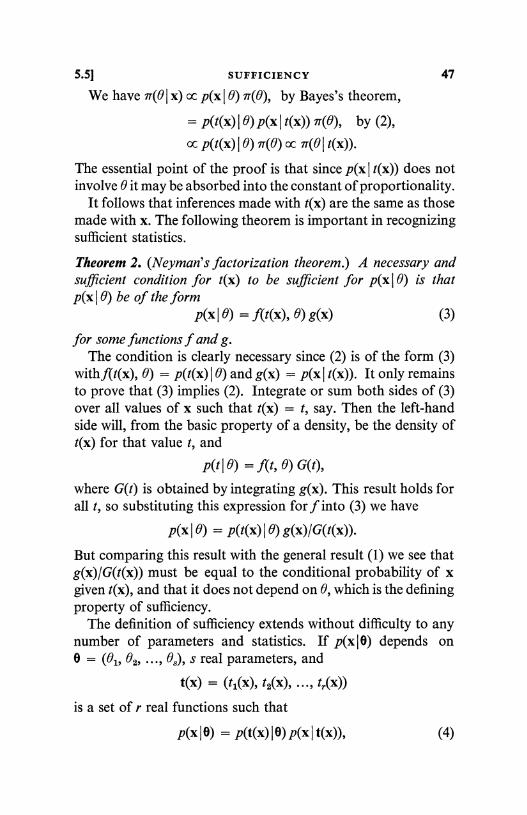
5.51 SUFFICIENCY 47
We have 7r(O I x) oc p(x 0) 7r(e), by Bayes's theorem,
= p(t(x) 6) p(x I t(x)) ir(e), by (2),Cc P(t(x) I e) 7r(6) Cc 7r(9 t(x)).
The essential point of the proof is that since p(x I t(x)) does notinvolve 0 it may be absorbed into the constant of proportionality.
It follows that inferences made with t(x) are the same as thosemade with x. The following theorem is important in recognizingsufficient statistics.
Theorem 2. (Neyman's factorization theorem.) A necessary andsufficient condition for t(x) to be sufficient for p(x10) is thatp(x 10) be of the form
p(x 0) = f(t(x), 0) g(x) (3)
for some functions f and g.The condition is clearly necessary since (2) is of the form (3)
withf(t(x), 0) = p(t(x) 0) and g(x) = p(x I t(x)). It only remainsto prove that (3) implies (2). Integrate or sum both sides of (3)over all values of x such that t(x) = t, say. Then the left-handside will, from the basic property of a density, be the density oft(x) for that value t, and
p(t B) = f(t, 0) G(t),
where G(t) is obtained by integrating g(x). This result holds forall t, so substituting this expression for f into (3) we have
p(x 10) = p(t(x) (e) g(x)/G(t(x)).
But comparing this result with the general result (1) we see thatg(x)/G(t(x)) must be equal to the conditional probability of xgiven t(x), and that it does not depend on 0, which is the definingproperty of sufficiency.
The definition of sufficiency extends without difficulty to anynumber of parameters and statistics. If p(x 16) depends on0 = (61i e2, ..., 0 ), s real parameters, and
t(x) = (tl(x), t2(x), ..., tr(x))
is a set of r real functions such that
Ax 10) = P(t(x) 10) Ax I t(x)), (4)
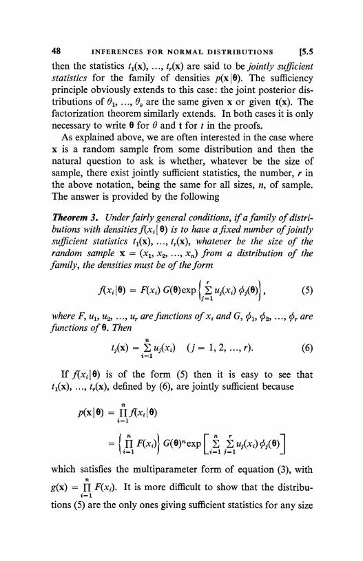
48 INFERENCES FOR NORMAL DISTRIBUTIONS [5.5
then the statistics tl(x), ..., t,(x) are said to be jointly sufficientstatistics for the family of densities p(x 18). The sufficiencyprinciple obviously extends to this case: the joint posterior dis-tributions of 0, ..., 0 are the same given x or given t(x). Thefactorization theorem similarly extends. In both cases it is onlynecessary to write 0 for 0 and t for t in the proofs.
As explained above, we are often interested in the case wherex is a random sample from some distribution and then thenatural question to ask is whether, whatever be the size ofsample, there exist jointly sufficient statistics, the number, r inthe above notation, being the same for all sizes, n, of sample.The answer is provided by the following
Theorem 3. Under fairly general conditions, if a family of distri-butions with densities f(xi 10) is to have a fixed number of jointlysufficient statistics t1(x), ..., t,(x), whatever be the size of therandom sample x = (x1, x2i ..., xn) from a distribution of thefamily, the densities must be of the form
ui(xi) O,(e)f(xi l e) = F(xi) G(e) exp IJ1
where F, u1i u2, ..., ur arefunctions of xi and G, 01, 02, ..., Or arefunctions of 6. Then
nt,(x) = E uj(xi) (j = 1, 2, ..., r). (6)
i=1
If f(xi 16) is of the form (5) then it is easy to see thattl(x), ..., tr(x), defined by (6), are jointly sufficient because
np(x
10)
= n f(xi l e)i=1
_ { H F(xi)} G(9)nexp [i fE uj(xi) 0;(e)]
which satisfies the multiparameter form of equation (3), withn
g(x) = rl F(xi). It is more difficult to show that the distribu-i=1
tions (5) are the only ones giving sufficient statistics for any size
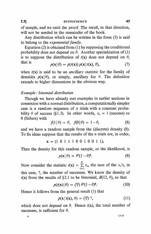
5.51 SUFFICIENCY 49
of sample, and we omit the proof. The result, in that direction,will not be needed in the remainder of the book.
Any distribution which can be written in the form (5) is saidto belong to the exponential family.
Equation (2) is obtained from (1) by supposing the conditionalprobability does not depend on 0. Another specialization of (1)is to suppose the distribution of t(x) does not depend on 0,that is p(x 10) = P(O)) Ax 10), 0), (7)
when t(x) is said to be an ancillary statistic for the family ofdensities p(x 0), or simply, ancillary for 0. The definitionextends to higher dimensions in the obvious way.
Example: binomial distributionThough we have already met examples in earlier sections in
connexion with a normal distribution, a computationally simplercase is a random sequence of n trials with a constant proba-bility 0 of success (§ 1.3). In other words, xi = 1 (success) or0 (failure) with
f(l 10) = 0, f(010) = 1- 0, (8)
and we have a random sample from the (discrete) density (8).To fix ideas suppose that the results of the n trials are, in order,
x=(101110010011).Then the density for this random sample, or the likelihood, is
P(x 10) = 01(1- 0)5. (9)
Now consider the statistic t(x) xi, the sum of the xi's, in= I
this case, 7, the number of successes. We know the density oft(x) from the results of §2.1 to be binomial, B(12, 0), so that
P(t(x)10) = (12) 617(1-0)5. (10)
Hence it follows from the general result (1) that
P(x I t(x), 0) = OD-11 (11)
which does not depend on 0. Hence t(x), the total number ofsuccesses, is sufficient for 0.
4 LS It
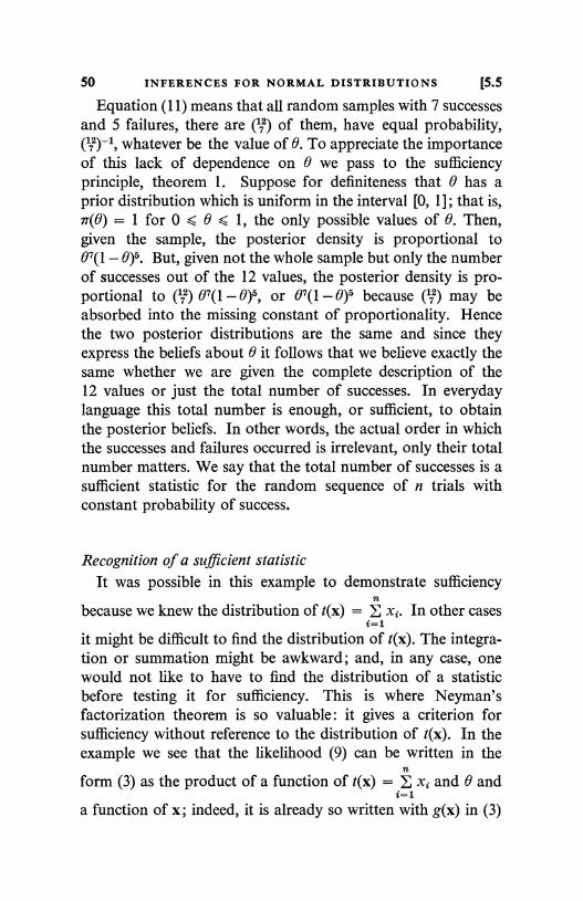
50 INFERENCES FOR NORMAL DISTRIBUTIONS [5.5
Equation (11) means that all random samples with 7 successesand 5 failures, there are (;2) of them, have equal probability,(11 )-1, whatever be the value of 0. To appreciate the importanceof this lack of dependence on 0 we pass to the sufficiencyprinciple, theorem 1. Suppose for definiteness that 0 has aprior distribution which is uniform in the interval [0, 1]; that is,n(0) = 1 for 0 5 0 < 1, the only possible values of 0. Then,given the sample, the posterior density is proportional to07(l - 0)5. But, given not the whole sample but only the numberof successes out of the 12 values, the posterior density is pro-portional to (72) 07(l - 0)5, or 07(l - 0)5 because (7) may beabsorbed into the missing constant of proportionality. Hencethe two posterior distributions are the same and since theyexpress the beliefs about 0 it follows that we believe exactly thesame whether we are given the complete description of the12 values or just the total number of successes. In everydaylanguage this total number is enough, or sufficient, to obtainthe posterior beliefs. In other words, the actual order in whichthe successes and failures occurred is irrelevant, only their totalnumber matters. We say that the total number of successes is asufficient statistic for the random sequence of n trials withconstant probability of success.
Recognition of a sufficient statisticIt was possible in this example to demonstrate sufficiency
nbecause we knew the distribution of t(x) = E x2. In other cases
2=1
it might be difficult to find the distribution of t(x). The integra-tion or summation might be awkward; and, in any case, onewould not like to have to find the distribution of a statisticbefore testing it for sufficiency. This is where Neyman'sfactorization theorem is so valuable: it gives a criterion forsufficiency without reference to the distribution of t(x). In theexample we see that the likelihood (9) can be written in the
nform (3) as the product of a function of t(x) _ xi and 0 and
i=1a function of x; indeed, it is already so written with g(x) in (3)
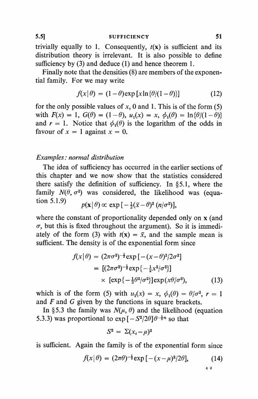
5.51 SUFFICIENCY 51
trivially equally to 1. Consequently, t(x) is sufficient and itsdistribution theory is irrelevant. It is also possible to definesufficiency by (3) and deduce (1) and hence theorem 1.
Finally note that the densities (8) are members of the exponen-tial family. For we may write
f(x 10) = (1- 0) exp [x In {0/(1- B)}] (12)
for the only possible values of x, 0 and 1. This is of the form (5)with F(x) = 1, G(8) = (1- 0), u,(x) = x, 0,(0) = In {8/(1- 0)}and r = 1. Notice that 0,(e) is the logarithm of the odds infavour of x = 1 against x = 0.
Examples: normal distributionThe idea of sufficiency has occurred in the earlier sections of
this chapter and we now show that the statistics consideredthere satisfy the definition of sufficiency. In §5.1, where thefamily N(8, 0"2) was considered, the likelihood was (equa-tion 5.1.9)
p(x 18) oc exp [ -i(x - 8)2
where the constant of proportionality depended only on x (andv, but this is fixed throughout the argument). So it is immedi-ately of the form (3) with t(x) = x, and the sample mean issufficient. The density is of the exponential form since
f(x 10) = exp [ - (X- 8)2/20'2]
= [(21!0"2)-I exp { - 2x2/2}77]
x [exp { - z exp (13)
which is of the form (5) with u,(x) = x, 0,(0) = 0/0.2, r = 1and F and G given by the functions in square brackets.
In §5.3 the family was N(,a, 0) and the likelihood (equation5.3.3) was proportional to exp [-S2 /20]0-In so that
S2 = F.(x; -,u)2
is sufficient. Again the family is of the exponential form since
f(x 8) = (21x8)-I exp [ - (x -,u)2/20], (14)42
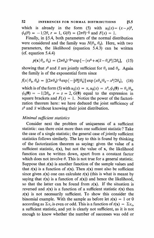
52 INFERENCES FOR NORMAL DISTRIBUTIONS [5.5
which is already in the form (5) with u1(x) = (x -,u)2,q1(0) _ - 1/20, r = 1, G(0) = (2ir0)-i and F(x) = 1.
Finally, in § 5.4, both parameters of the normal distributionwere considered and the family was N(01, 02). Here, with twoparameters, the likelihood (equation 5.4.3) can be written(cf. equation 5.4.4)
P(x 1 01, 02) _ (2n02)-in exp [ - {VS2 + n(x - 01)2}/202], (15)
showing that s2 and x are jointly sufficient for 01 and 02. Againthe family is of the exponential form since
f(x 101, 02) = [(2ir02)-i exp { - z 0;/02}] exp {x01/02 - x2/202}, (16)
which is of the form (5) with u1(x) = x, u2(x) = x2, X1(8) = 01/02,c2(0) = - 1/202i r = s = 2, G(e) equal to the expression insquare brackets and F(x) = 1. Notice the power of the factori-zation theorem here: we have deduced the joint sufficiency ofs2 and x without knowing their joint distribution.
Minimal sufficient statisticsConsider next the problem of uniqueness of a sufficient
statistic: can there exist more than one sufficient statistic? Takethe case of a single statistic; the general case of jointly sufficientstatistics follows similarly. The key to this is found by thinkingof the factorization theorem as saying: given the value of asufficient statistic, t(x), but not the value of x, the likelihoodfunction can be written down, apart from a constant factorwhich does not involve 0. This is not true for a general statistic.Suppose that s(x) is another function of the sample values andthat t(x) is a function of s(x). Then s(x) must also be sufficientsince given s(x) one can calculate t(x) (this is what is meant bysaying that t(x) is a function of s(x)) and hence the likelihood,so that the latter can be found from s(x). If the situation isreversed and s(x) is a function of a sufficient statistic t(x) thens(x) is not necessarily sufficient. To show this consider thebinomial example. With the sample as before let s(x) = 1 or 0according as Exi is even or odd. This is a function of t(x) = Exi,a sufficient statistic, and yet is clearly not sufficient, as it is notenough to know whether the number of successes was odd or
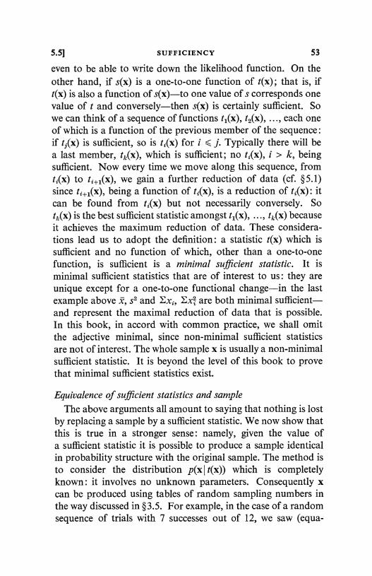
5.51 SUFFICIENCY 53
even to be able to write down the likelihood function. On theother hand, if s(x) is a one-to-one function of t(x) ; that is, ift(x) is also a function of s(x)-to one value of s corresponds onevalue of t and conversely-then s(x) is certainly sufficient. Sowe can think of a sequence of functions ta(x), t2(x), ..., each oneof which is a function of the previous member of the sequence:if t;(x) is sufficient, so is ti(x) for i 5 j. Typically there will bea last member, tk(x), which is sufficient; no ti(x), i > k, beingsufficient. Now every time we move along this sequence, fromti(x) to ti+1(x), we gain a further reduction of data (cf. §5.1)since ti}1(x), being a function of ti(x), is a reduction of ti(x) : itcan be found from ti(x) but not necessarily conversely. Sotk(x) is the best sufficient statistic amongst tl(x), ..., tk(x) becauseit achieves the maximum reduction of data. These considera-tions lead us to adopt the definition: a statistic t(x) which issufficient and no function of which, other than a one-to-onefunction, is sufficient is a minimal sufficient statistic. It isminimal sufficient statistics that are of interest to us: they areunique except for a one-to-one functional change-in the lastexample above x, s2 and Exi, Exi are both minimal sufficient-and represent the maximal reduction of data that is possible.In this book, in accord with common practice, we shall omitthe adjective minimal, since non-minimal sufficient statisticsare not of interest. The whole sample x is usually a non-minimalsufficient statistic. It is beyond the level of this book to provethat minimal sufficient statistics exist.
Equivalence of sufficient statistics and sampleThe above arguments all amount to saying that nothing is lost
by replacing a sample by a sufficient statistic. We now show thatthis is true in a stronger sense: namely, given the value ofa sufficient statistic it is possible to produce a sample identicalin probability structure with the original sample. The method isto consider the distribution p(x I t(x)) which is completelyknown: it involves no unknown parameters. Consequently xcan be produced using tables of random sampling numbers inthe way discussed in § 3.5. For example, in the case of a randomsequence of trials with 7 successes out of 12, we saw (equa-
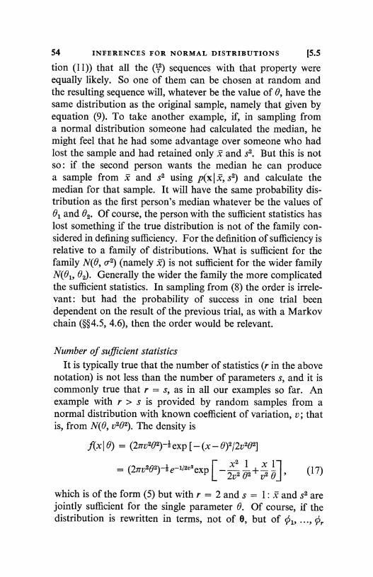
54 INFERENCES FOR NORMAL DISTRIBUTIONS [5.5
tion (11)) that all the (;2) sequences with that property wereequally likely. So one of them can be chosen at random andthe resulting sequence will, whatever be the value of 0, have thesame distribution as the original sample, namely that given byequation (9). To take another example, if, in sampling froma normal distribution someone had calculated the median, hemight feel that he had some advantage over someone who hadlost the sample and had retained only x and s2. But this is notso: if the second person wants the median he can producea sample from x and s2 using p(x I X, s2) and calculate themedian for that sample. It will have the same probability dis-tribution as the first person's median whatever be the values of01 and 02. Of course, the person with the sufficient statistics haslost something if the true distribution is not of the family con-sidered in defining sufficiency. For the definition of sufficiency isrelative to a family of distributions. What is sufficient for thefamily N(9, 0.2) (namely x) is not sufficient for the wider familyN(01, 02). Generally the wider the family the more complicatedthe sufficient statistics. In sampling from (8) the order is irrele-vant: but had the probability of success in one trial beendependent on the result of the previous trial, as with a Markovchain (§§4.5, 4.6), then the order would be relevant.
Number of sufficient statisticsIt is typically true that the number of statistics (r in the above
notation) is not less than the number of parameters s, and it iscommonly true that r = s, as in all our examples so far. Anexample with r > s is provided by random samples from anormal distribution with known coefficient of variation, v; thatis, from N(0, v202). The density is
f(x J9) _ (2mrv202)-I exp [ - (x - 0)2/2v202]
_ (21rv202)-l: e-1/2)2eXp - x21 + x 1 (17)2v2 02 y2 B]
which is of the form (5) but with r = 2 and s = 1: h and s2 arejointly sufficient for the single parameter 0. Of course, if thedistribution is rewritten in terms, not of 9, but of 01, ..., ¢,.
5.5] SUFFICIENCY 55
(equation (5)), then necessarily the numbers of statistics andparameters are equal.
Exponential family
Two comments on theorem 3 are worth making. Supposewe are sampling from an exponential family with prior distribu-tion 7r(B) and consider the way in which the beliefs change withthe size of sample. We suppose, purely for notational simplicity,that r = s = 1 so that
f(xi 0) = F(xi) G(0) exp [u(xi) ¢(0)].
Then 7r(0 I x) cc ir(0) G(0)nexp [t(x) 0(0)], (18)n
with t(x) _ u(xi), after a random sample of size n. As n and
t(x) change, the family of densities of 0 generated by (18) can bedescribed by two parameters, n and t(x). This is because thefunctional form of 7r(0 I x) is always known, apart from thesevalues. Consequently the posterior distribution always belongsto a family dependent on two parameters, one of which, n,changes deterministically, and the other, t(x), changes randomlyas sampling proceeds. In sampling from an exponential familythere is thus a natural family of distributions of 0 to consider;namely that given by (18). Furthermore, it is convenient tochoose 9r(0) to be of the form G(0)aebo(O), for suitable a and b,because then the prior distributions fit in easily with the likeli-hood. This is part of the reason for the choice of prior distribu-tions in theorems 5.1.1 and 5.3.1. For general r and s, the jointposterior density of the s parameters depends on (r+ 1)
nparameters, n and the statistics u;(xi).
i=1The distributions (18) are said to belong to the family which
is conjugate to the corresponding member of the exponentialfamily. The nomenclature is due to Raiffa and Schlaifer (1961).One advantage in using the conjugate family is that methodsbased on it essentially reduce to the methods appropriate tovague prior knowledge, like most of the methods developedin this book. The point has been mentioned in § 5.2 and examplesare available in the alternative proof of theorem 6.6.1 and in
56 INFERENCES FOR NORMAL DISTRIBUTIONS [5.5
§ 7.2. If we have samples from the exponential family (still con-sidering r = s = 1) and decide the prior distribution isadequately represented by the conjugate distribution (18) withn = a, t(x) = b, then the observations are adequately sum-
pmarized by the sample size, n, and u(xi), and the posterior
distribution is of the conjugate family with parameters a + n andn
b + u(xi). This posterior distribution is equivalent to that
which would have been obtained with a sample of size a + nn
yielding sufficient statistic b + u(xi) with prior knowledgez=
7r(O) (in (18)). If ir(©) corresponds to vague prior knowledge, wemay use the methods available for that case.
Regularity conditions
A second comment on theorem 3 concerns the first few words`under fairly general conditions'. We have no wish to weary thereader with the precise conditions, but the main conditionrequired for the result to obtain is that the range of the distribu-tion does not dependt on 0. If the range is a function of 0 thenthe situation can be quite different even in simple cases. Con-sider, for example, a uniform distribution in the interval (0, 0)with, as usual, 0 as the unknown parameter. Here
f(xi 10) = 61-1, 0 <, xi 5 0;and is otherwise zero, and
p(x 10) = 0-n, if 0 < xi < 0 for all i;and is otherwise zero. Consequently the likelihood is 0-n,provided 0 > max xi, and is otherwise zero. Hence the likeli-
hood depends only on max xi which is sufficient, and yet the
density is not of the exponential family. Difficulties of this sortusually arise where the range of possible values of the randomvariable depends on the unknown parameter. In the other casesstudied in this chapter the range is the same for all parametervalues.
t Readers familiar with the term may like to know that difficulties arise whenthe distributions are not absolutely continuous with respect to each other.
5.51 SUFFICIENCY 57
Ancillary statisticsAncillary statistics do not have the same importance as
sufficient statistics. Their principal use is to say that the distri-bution of t(x) is irrelevant to inferences about 0, because thelikelihood, p(x 10), is proportional to p(x I t(x), 0). In otherwords, t(x) may be supposed constant. Important examples oftheir use are given in theorems 7.6.2 and 8.1.1. A simpleexample is provided by considering a scientist who wishes totake a random sample from a distribution with density f(xI0).Suppose that the size of the random sample he is able to takedepends upon factors such as time at his disposal, moneyavailable, etc.: factors which are in no way dependent on thevalue of 0, but which may determine a probability density, p(n),for the sample size. Then the density of the sample is given by
p(x 19) = p(n) II f(x, 10).2=1
It follows that t(x) = n is an ancillary statistic. Consequentlythe scientist can suppose n fixed at the value he actually obtainedand treat the problem as one of a random sample of fixed sizefrom f(x 10). In particular, if f(x 10) is normal, the methods ofthis chapter will be available.
Nuisance parametersFinally, notice something that has not been defined. If there
is more than one parameter; say two, e1 and 02, we have notdefined the notion of statistics sufficient or ancillary for one ofthe parameters, 01i say, when 02 is a nuisance parameter. Nosatisfactory general definition is known. For example, it is nottrue that, in sampling from N(01, 02), x is sufficient for 01i forthe posterior distribution of 61 involves s, so without it the dis-tribution could not be found. However, something can be done.Suppose (cf. (1))
p(x 101, 02) = p(t(x) 101, 02)p(x I t(x), 02), (19)
so that B1 is not present in the second probability on the right-hand side. Then, given 02i t(x) is sufficient for 81: for, if 02 were
58 INFERENCES FOR NORMAL DISTRIBUTIONS [5.5
known the only unknown parameter is 01 and (2) obtains. Sowe can speak of sufficiency for one parameter, given the other.In the normal example just cited x is sufficient for 01, given 02.
Similarly, if
P(x 181, 02) = P(t(x)1 02) P(x 10), 01, 02), (20)
then, given 02, t(x) is ancillary for 01. Hence it is possible tospeak of ancillary statistics for one parameter given the other.If (19) can be specialized still further to
P(x 1011 02) = P(t(x)10l) p(x 10), 02), (21)
then, given 02, t(x) is sufficient for 01; and, given 01, t(x) isancillary for 02.
Both the original definitions made no mention of priorinformation, but if this is of a particular type then further con-sequences emerge. Suppose, with a likelihood given by (21),01 and 02 have independent prior distributions. The posteriordistribution is then
i(Bl, 021 x) CC [PO(x) 101) g(001 [p(x 10), 02) 77(02)], (22)
and 0l and 02 are still independent. Furthermore, if only thedistribution of 0l is required t(x) provides all the information:if only that of 02 is required, then t(x) may be supposed constant.Or, for independent prior distributions, t(x) is sufficient for 01and ancillary for 02. But unlike the usual definitions of sufficientand ancillary statistics these depend on certain assumptionsabout the prior distribution.
5.6. Significance tests and the likelihood principleSuppose we have some data, x, whose distribution depends
on several parameters, 01, 02, ..., 0, and that some value of 01,denoted by 91, is of special interest to us. Let the posteriordensity of 0l be used to construct a confidence interval for 01with coefficient fl (on data x). If this interval does not containthe value 01 then the data tend to suggest that the true value of01 departs significantly from the value 01 (because 01 is not con-tained in the interval within which one has confidence that thetrue value lies) at a level measured by a = 1-,6. In these
5.61 SIGNIFICANCE TESTS 59
circumstances we will say the data are significant at the a level;a is the level of significance and the procedure will be called asignificance test. The statement that 91 = , is called the nullhypothesis. Any statement that 01 = Bl + Bl is an alternativehypothesis. The definitions extend to any subset of the para-meters 01, 02, ..., 0 with u < s using the joint confidence set of0, ..., 0 , and values B1, ..., V.. An alternative interpretation ofa confidence interval is an interval of those null hypotheseswhich are not significant on the given data at a prescribedsignificance level a = 1-,d.
The likelihood principleIf two sets of data, x and y, have the following properties :(i) their distributions depend on the same set of parameters;(ii) the likelihoods of these parameters for the two sets are
the same;(iii) the prior densities of the parameters are the same for the
two sets;then any statement made about the parameters using x shouldbe the same as those made using y.
The principle is immediate from Bayes's theorem because theposterior distributions from the two sets will be equal.
Example of a significance testLike the closely related concept of a confidence interval a
significance test is introduced for practical rather than mathe-matical convenience. Consider the situation of § 5.1, where thedata are samples from N(O, o-2), so that there is only one para-meter, and consider in particular the numerical illustrationon the measurement of conductivity of an insulating material,with the uniform prior distribution (oro --> oo). There may wellbe a standard laid down to ensure that the conductivity is nottoo high: for example that the conductivity does not exceed17, otherwise the insulation properties would be unsatisfactory.This value of 17 is the value 0 referred to in the definition: thenull hypothesis. The main interest in the results of the experi-ment lies in the answer to the question: `Is the conductivitybelow 17?' If it is, the manufacturer or the inspector (or the
60 INFERENCES FOR NORMAL DISTRIBUTIONS [5.6
consumer) probably does not mind whether it is 15 or 16.Consequently the main feature of the posterior distribution thatmatters is its position relative to the value 17. Let us first con-sider the reasonableness of 17 as a possible value of the con-ductivity. The 95 % confidence interval for the mean is16.57 ± 1.96 x (1/,I10); that is (15.95, 17.19) so that we can saythat the true conductivity, granted that the measuring instru-ment is free from bias, most likely lies in this interval. But thisinterval includes the value 17 so it is possible that this materialdoes not meet the specification. In the language above, theresult is not significant at the 5 Y. level. Had an 80 % confidenceinterval been used the values would have been (16.17, 16.97),since (D(- 1-28) = 0.10 (cf. equation 2.5.14). This does notinclude the value 17 so that the result is significant at the 20level. This is not normally regarded as a low enough level ofsignificance. The values 5, 1 and 0.1 % are the levels commonlyused, because they provide substantial amounts of evidence thatthe true value is not 01, when the result is significant. Occasion-ally the exact significance level is quoted: by this is meant thecritical level such that levels smaller than it will not give signifi-cance, and values above it will. In the numerical example werequire to find a such that
16.57+Aa(1/Vl0) = 17, (1)
) = a : or, in the language of § 5.3, A, is thewhere 2(D(-;t,upper Ja point of the standardized normal distribution. From(1) the value of A is 1.36 and the tables show that
1(-1.36) = 0.087,
so that a = 0.174. The result is just significant at the level,17.4 %. This agrees with what we have just found: the result issignificant at 20 % but not at 5 %.
Just as there is some arbitrariness about a confidence interval,so there must be arbitrariness about a significance test (cf. § 5.2).Thus, in this example, we could have used a one-sided confidenceinterval from - oo to some value and defined significance withrespect to it. Indeed this might be considered more appropriatesince all we want to do is to be reasonably sure that the true
5.6] SIGNIFICANCE TESTS 61
value does not exceed 17. At the 5 % level this interval extendsto 16.57+ 1.64 (1/x/10) = 17.09 so we think that the conductivityis most likely less than 17.09 which would not normally beenough evidence to dismiss the doubts that the conductivitymight exceed 17. If this test is used the exact significance levelis the posterior probability that 0 exceeds 17. Since 0 isN(16.57, 0.1) this value is
1-(D
1 6.57)1- D(1.36) =
(17.OO_1/x/10
(compare the calculation above) so that the exact significancelevel is 8.7 %, half what it was with the symmetric shortestconfidence interval. In this example this is probably the bestway of answering the question posed above: by quoting therelevant posterior probability that the material is unsatisfactoryand avoiding significance level language completely. There isdiscernible in the literature a tendency for significance tests to bereplaced by the more informative confidence intervals, and thisseems a move in the right direction.
It must be emphasized that the significance level is, even morethan a confidence interval, an incomplete expression of posteriorbeliefs. It is used because the complete posterior distribution istoo complicated. A good example of its use will be found in§8.3 where many parameters are involved. In the simple casesso far discussed there seems no good reason for using significancetests.
Prior knowledge
The type of significance test developed here is only appro-priate when the prior knowledge of 0 is vague (in the sense dis-cussed in § 5.2). In particular, the prior distribution in theneighbourhood of the null value B must be reasonably smoothfor the tests to be sensible. In practical terms this means thatthere is no reason for thinking that 0 = 0 any more than anyother value near B. This is true in many applications, but thereare situations where the prior probability that 0 = B is appreci-ably higher than that for values near B. For example, if 0 is theparameter in genetics that measures the linkage between two
62 INFERENCES FOR NORMAL DISTRIBUTIONS [5.6
genes, the value 0 = 0 = 0 corresponds to no linkage, meaningthat the genes are on different chromosomes; whereas 0 near 0means that there is some linkage, so that the genes are on thesame chromosome, but relatively well separated on it. In thiscase the prior distribution may be of the mixed discrete andcontinuous type with a discrete concentration of probabilityon 0 = 0 and a continuous distribution elsewhere. The relevantquantity to consider here is the posterior probability that 0 = 0.Significance tests of this type have been considered by Jeffreys(1961) but are not much used. They will not be mentionedfurther in this book, but their introduction provides a furtheropportunity to remind the reader that the methods developedin this book are primarily for the situation of vague priorknowledge, and have to be adapted to take account of otherpossibilities (see, for example, §7.2).
Decision theoryIt is also well to notice what a significance test is not. It is not
a recipe for action in the sense that if a result is significant thenone can act with reasonable confidence (depending on the level)as if 0 was not B. For example, the manufacturer of insulatingmaterial may not wish to send to his customers any materialwith 0 > 17. Since he does not know 0 exactly he may have todecide whether or not to send it on the evidence of the data. Hetherefore has to act in one of two ways : to send it to the customeror to retain it for further processing, without exact knowledgeof 0. We often say he has to take one of two decisions. Theproblem of action or decision is not necessarily answered byretaining it if the test is significant. The correct way to decide isdiscussed in decision theory: which is a mathematical theory ofhow to make decisions in the face of uncertainty about the truevalue of parameters. The theory will not be discussed in detailin this book but since it is so closely related to inference a briefdescription is not out of place.
The first element in decision theory is a set of parameters 0which describes in some way the material of interest and aboutwhich the decisions have to be made. In the conductivityexample there is a single parameter, namely the conductivity,
5.61 SIGNIFICANCE TESTS 63
and it is required to decide whether or not it exceeds 17 in value.The second element is a set of decisions d which contains all thepossible decisions that might be taken. In the example there aretwo decisions, to despatch or retain the material. Notice that theset of decisions is supposed to contain all the decisions thatcould be taken and not merely some of them: or to put itdifferently, we have, in the theory, to choose amongst a numberof decisions. Thus it would not be a properly defined decisionproblem in which the only decision was whether to go to thecinema, because if the decision were not made (that is, one didnot go to the cinema) one would have to decide whether to stayat home and read, or go to the public-house, or indulge in otheractivities. All the possible decisions, or actions, must be includedin the set. Our example is probably inadequate in this respectsince it does not specify just what is going to happen if thematerial is to be rejected. Is it, for instance, to be scrappedcompletely or to be reprocessed?
The two elements, the decisions d and the parameters 0, arerelated to one another in the sense that the best decision to takewill depend on the value of the parameter. In the example it willclearly be better to reject if 0 > 17 and otherwise accept. Wenow discuss the form the relationship must take. If 0 wereknown then clearly all that is needed is a knowledge of the bestdecision for that value of 0. But decision theory deals with thecase where 0 is unknown : it can then be shown that a relation-ship of such a form, namely knowing the best d for each 0,between d and 0 is inadequate. This can be seen in the example:one could only expect to be able to make a sensible decision ifone knew how serious it was to retain material whose con-ductivity was below 17, and to despatch material to the customerwhose conductivity was in excess of 17. If the latter was notserious the manufacturer might argue that he could `get awaywith it' and send out material of inadequate insulation. If theseriousness were changed, for example by the introduction ofa law making it an offence to sell material of conductivity inexcess of 17, he might well alter his decision.
A relationship between d and 0 stronger than knowledge ofthe best d for each 0 is required. It has been shown (see § 1.6)
64 INFERENCES FOR NORMAL DISTRIBUTIONS [5.6
that the relationship can always be described in the followingway. For each pair of values, d and 0, there is a real numberU(d, 0) called the utility of making decision d when the truevalue is 9. U(d, 0) is called a utility function. It describes, ina way to be elaborated on below, the desirability or usefulness ofthe decision d in the particular set of circumstances describedby 0. In particular, the value of d which maximizes U(d, 0) fora fixed 0 is the best decision to take if the situation is knownto have that value of 9. Generally if U(d, 0) > U(d', 0) then,if 0 obtains, d is preferred to d'. In the example, where 0 = 0 isthe conductivity, d is the decision to despatch and d' to retain,a utility function of the following form might be appropriate, atleast in the neighbourhood of 0 = 17:
U(d, 0) = a + c(B - 0),
U(d', 0) = a + c'(0 - B),
where a, c and c' are positive constants. Then, for 0 > 0,U(d', 0) > U(d, 0) so that it is best to retain; and for 0 < 0 theopposite inequality obtains and it is best to despatch. Notice thatif 0 differs from B by an amount h, say, in either direction, thenthe two utilities differ by the same amount, namely (c+c')h.Consequently, the mistake of retention when 0 = -0-h is justas serious (in the sense of losing utility) as is the mistake ofdespatch when 0 = 0 + h. This would probably not be reasonableif there was a law against marketing insulating material of anunsatisfactory nature: the mistake of despatching poor materialmight then involve more serious consequences than that ofretaining good workmanship.
The scale upon which utility is to be measured has to becarefully considered. In particular, consider what is meant bysaying that one course of action has twice the utility of another.Specifically, in a given set of circumstances, defined by 0, let dland d2 be two courses of action with utilities 1 and 2 respectively,and let do be a course of action with utility zero. Suppose thatbetween do and d2 the course of action is chosen by the toss ofa fair coin. If it falls heads then do is taken, if it falls tails then d2is taken. The expected utility (in the usual sense of expectation)is half the utility of do plus half the utility of d2, or 1.0 + 1.2 = 1.
5.6] SIGNIFICANCE TESTS 65
Hence this random choice between do and d2 has the sameexpected utility as d1, namely 1, and the random choice is con-sidered as of the same usefulness as d1. In other words, onewould be indifferent between d1 and the random choice betweendo and d2. Utility is measured on a scale in which the certaintyof 1 is as good as a fifty-fifty chance of 2 or 0. There would benothing inconsistent in saying that the utility of obtaining £1was 1 but that of obtaining £2 was 12, for an evens chance of £2(yielding utility, ) may not be considered as desirable as thecertainty of £1. Utility is not necessarily the same as money.
The discussion of the utility scale shows how the utility canbe used to arrive at a decision in a sensible manner when thetrue value of 0 is not completely known. The important quantityis the expected utility. If there is some uncertainty about 0 itfollows, from our earlier considerations, that there exists aprobability distribution for 0, and hence we need to considerthe expected utility, where the expectation is with respect to thisdistribution. Let n(0) denote our knowledge of 0 expressed inthe usual way as a probability density. The expected utility ofa decision d is then, by definition,
JU(d, 0) n(O) A = U(d), (2)
say. The best decision to take is that which maximizes U(d).In the example of a utility function cited above the expectedutility of despatch is
U(d) = a+J c(6-0)nr(0)dO = a+c(O-01)
and of retention is a + c'(01- V), where 01 is the expected valueof 0, or the mean of the density 1T(0). U(d) > U(d') if 01 < 0.Hence the material is despatched if the expected value of 0is below the critical value. This is sensible because, as weremarked, mistakes on either side of the critical value areequally serious with this utility function.
It remains to discuss the role of observations in decisiontheory. Suppose that a set of observations, x, is obtained andthat, as a result, the knowledge of 0 is changed by Bayes'stheorem to the posterior distribution given x, 1T(0 lx). The
5 LSII
66 INFERENCES FOR NORMAL DISTRIBUTIONS [5.6
decision must now be made according to the new expectedutility
f J U(d, A) ir(A x) dA = U(d, x), (3)
say; that decision being taken which maximizes this quantity.On intuitive grounds one expects the decision made on thebasis of (3) to be better than that made using (2), for otherwisethe observations have not been of any value. This feeling isexpressed mathematically by saying that the expected value ofthe maximum of (3) exceeds the maximum of (2). The expectedvalue is
fmax U'(d, x) 7r(x) dx, (4)a
where 71(x) is the distribution of x anticipated before the obser-vations were made : that is, in the light of the prior knowledgeconcerning 0. (Compare the discussion on beliefs about thesample in § 5.1.) Precisely
rr(x) = fp(x I A)1r(O) dA,
where p(x 10) is the density of the observation given 0 in theusual way. This mathematical result is easily established.
Inference and decision theoryThe reader is referred to the list of suggestions for further
reading if he wishes to pursue decision theory beyond this briefaccount. It should be clear that the inference problem discussedin the present book is basic to any decision problem, becausethe latter can only be solved when the knowledge of 0 isadequately specified. The inference problem is just the problemof this specification: the problem of obtaining the posteriordistribution. Notice that the posterior distribution of 0 thatresults from an inference study is exactly what is required tosolve any decision problem involving A. The role of inference isto provide a statement of the knowledge of 0 that is adequatefor making decisions which depend on A. This it does byproviding the posterior distribution either in its entirety or insome convenient summary form, such as a confidence statement.
5.6] SIGNIFICANCE TESTS 67
The person making the inference need not have any particulardecision problem in mind. The scientist in his laboratory doesnot consider the decisions that may subsequently have to bemade concerning his discoveries. His task is to describe accu-rately what is known about the parameters in question.
[The remainder of this section is not necessary for an under-standing of the rest of the book. It is included so that theperson who learns his statistics from this book can understandthe language used by many other scientists and statisticians.]
Non-Bayesian significance testsThe concept of a significance test is usually introduced in
a different way and defined differently. We shall not attempt ageneral exposition but mainly consider the significance test fora normal mean when the variance is known, the case just dis-cussed numerically. This will serve to bring out the major pointsof difference. Suppose, then, that we have a random sample ofsize n from N(O, o.2) and we wish to test the null hypothesis that0 = 0. The usual argument runs as follows. Since x is sufficientit is natural to consider it alone, without the rest of the data.x is known to have a distribution which is N(ia, 0-2 In) if It isthe true, but unknown, value of 0 (cf. §§3.3, 3.5). Suppose thetrue value is the null hypothesis value, d, then x is N(B, o-2/n)and so we can say that, with probability 0.95, n will lie withinabout 2o-/Vn of 0. (Notice that this probability is a frequencyprobability, and is not normally thought of as a degree of belief.)Hence we should be somewhat surprised, if ,u were 0, to have xlie outside this interval. If it does lie outside then one of twothings must have happened : either (i) an event of small prob-ability (0.05) has taken place, or (ii) ,u is not 0. If events of smallprobability are disregarded then the only possibility is that u isnot 0. The data would seem to signify, whenever x differs from 0by more than 2o]/Vn, that ,u is not 0, the strength of the signifi-cance depending on the (small) probability that has beenignored. Hence, if l2- 01 > 2o-/.fin, it is said that the result issignificant at the 5 % level. Notice that this interval is exactlythe same as that obtained using Bayes's theorem and confidenceintervals to construct the significance test: for the confidence
5-2
68 INFERENCES FOR NORMAL DISTRIBUTIONS [5.6
interval for 0 is x ± 2o/Vn. This identification comes from theparallelism between (a) and (b) in §5. 1.
The general procedure, of which this is an example, is to takea statistic t(x), which is not necessarily, or even usually, suffi-cient; to find the probability distribution of t(x) when 01 = 01and to choose a set of values of t(x) which, when 01 = 01, aremore probable under some plausible alternative hypotheses thanunder the null hypothesis. If the observed value of t(x) belongsto this set then, either 01 = 01 and an improbable event hasoccurred, or 01 + 0,. The result is said to be significant at a levelgiven by the probability of this set. There exists a great deal ofliterature on the choice of t(x) and the set. Confidence limitscan be obtained from significance tests using the alternativedefinition of the limits given above.
There are many criticisms that can be levelled against thisapproach but we mention only two. First, the probabilityquoted in the example of a significance test is a frequencyprobability derived from random sampling from a normal dis-tribution : if one was to keep taking samples from the distribu-tion the histogram of values of x obtained would tend toN(0, o.2/n). But the interpretation of the probability is in termsof degree of belief, because the 5 %, or 1 %, is a measure ofhow much belief is attached to the null hypothesis. It is used asif 5 % significance meant the posterior probability that 0 isnear 0 is 0.05. This is not so: the distortion of the meaning isquite wrong in general. It may, as with N(0, 0-2), be justifiable,but this is not always so.
Significance tests and the likelihood principleThe second criticism is much more substantial. The use of
significance tests based on the sampling distribution of astatistic t(x) is in direct violation of the likelihood principle.The principle is self-evident once it has been admitted thatdegrees of belief obey the axioms of probability; yet its practicalconsequences are far-reaching. Since it is not our purpose toprovide an account of significance tests based on the samplingdistribution of a statistic we shall use an example to show howthe usual significance test violates the likelihood principle. Our
5.61 SIGNIFICANCE TESTS 69
example may seem a little curious but this is because it isnecessary to take a case where the choice of t(x) is unambiguousso that there is no doubt about the significance test and there-fore about the significance level. We shall quote the exact leveldefined above.
Suppose a random sample of one is taken from B(4, 0): orequivalently we have a random sequence of four trials withconstant probability, 0, of success. By the sufficiency argumentonly x, the number of successes is relevant, so that x maytake one of 5 values: 0, 1, 2, 3, 4. Suppose scientist 1 canobserve the value of x. Suppose scientist 2 can merely observewhether the number of successes is 1, or not: in other words, hewill observe A if x = 1 and A if x is 0, 2, 3 or 4. Now let themobserve the same random value and suppose scientist 2 observesA and therefore scientist 1 observes x = 1, so that they bothhave the same information. (Of course, had scientist 2 observedA, they would not have been similarly placed, but that isirrelevant.) Then the likelihood for both scientists is 40(1- 0)3and hence, by the likelihood principle their inferences should bethe same. Nevertheless, had the above type of significance testbased on a sampling distribution been used with 0 = I as thenull hypothesis and J < 0 < I as the alternatives, scientist 1would have declared the result significant at 500/16 Y. andscientist 2 at 400/16 %. The explanation of the difference is thatscientist 1 would have included the points 0 and 1 in the set ofvalues, whereas scientist 2 would only have included A. When0 = Z, scientist l's set has probability 1/16+4/16 = 5/16,whereas scientist 2's set has probability 4/16. Larger differencescould be obtained with numerically more complicated examples.
Similar objections can be raised to confidence intervalsderived from such significance tests and that is why they are notused in this book. Nevertheless, in the situations commonlystudied in statistics the results given here agree with thoseobtained by other methods. The reason is the existence ofparallel properties of t(x) and 0 similar to those mentioned in§5.1 ((a) and (b)). Only in §6.3 will there be a case where theresults are different.
70 INFERENCES FOR NORMAL DISTRIBUTIONS [5.6
Suggestions for further reading
As already stated in the text the treatment of statistics adoptedin this book is unorthodox in that the approach is unusual,though the results are broadly the same as provided by theusual methods. Every reader ought to look at one of theorthodox books. He will find much overlap with our treat-ment, though a few topics (like unbiased, minimum varianceestimation) which loom large in those books receive littleattention here, and others (like posterior distributions) arescarcely considered by the orthodox school. The two approachescomplement each other and together provide a substantiallybetter understanding of statistics than either approach on itsown. Among the orthodox books at about the level of thepresent one mention can be made of Alexander (1961), Birn-baum (1962), Brunk (1960), Hogg and Craig (1959), Hoel (1960),Tucker (1962) and Fraser (1958).
Statistics is essentially a branch of applied mathematics in theproper' meaning of the word `applied' and no satisfactoryunderstanding of the subject can be obtained without someacquaintance with the applications. These have largely beenomitted from the present work, for reasons explained in thepreface, so that every reader ought to look at at least one bookwritten, not for the mathematician, but for the user of statistics.The number of these is legion and cover applications to almostevery branch of human knowledge. We mention only one whichseems extremely good, that edited by Davies (1957).
Little statistical work is possible without a set of tables of themore common distributions. A small set, adequate for most ofthe methods described in this book is that by Lindley andMiller (1961). Two larger collections are those by Fisher andYates (1963) and Pearson and Hartley (1958). An index tostatistical tables has recently been issued by Greenwood andHartley (1962).
The field of decision theory is covered in two books, Schlaifer(1959) and Raiffa and Schlaifer (1961), along Bayesian lines,
t As distinct from its meaning in the subject Applied Mathematics as taughtin British Universities, which is confined to applications to physics.
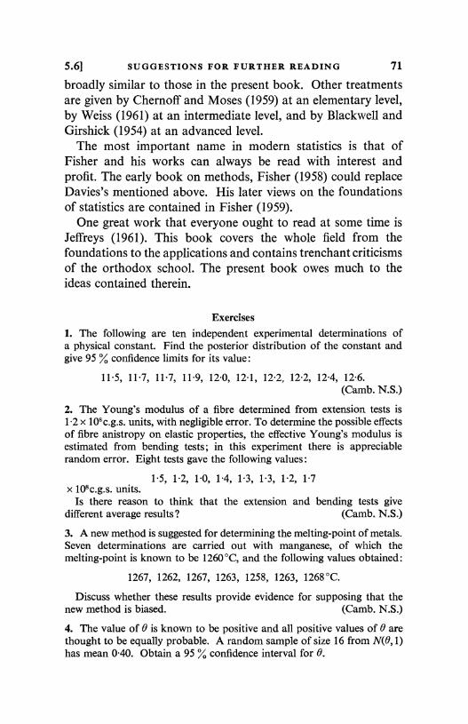
5.61 SUGGESTIONS FOR FURTHER READING 71
broadly similar to those in the present book. Other treatmentsare given by Chernoff and Moses (1959) at an elementary level,by Weiss (1961) at an intermediate level, and by Blackwell andGirshick (1954) at an advanced level.
The most important name in modern statistics is that ofFisher and his works can always be read with interest andprofit. The early book on methods, Fisher (1958) could replaceDavies's mentioned above. His later views on the foundationsof statistics are contained in Fisher (1959).
One great work that everyone ought to read at some time isJeffreys (1961). This book covers the whole field from thefoundations to the applications and contains trenchant criticismsof the orthodox school. The present book owes much to theideas contained therein.
Exercises
1. The following are ten independent experimental determinations ofa physical constant. Find the posterior distribution of the constant andgive 95 % confidence limits for its value:
11.5, 11.7, 11.7, 11.9, 12.0, 12.1, 12.2, 12.2, 12.4, 12.6.(Camb. N.S.)
2. The Young's modulus of a fibre determined from extension tests is1.2 x 108c.g.s. units, with negligible error. To determine the possible effectsof fibre anistropy on elastic properties, the effective Young's modulus isestimated from bending tests; in this experiment there is appreciablerandom error. Eight tests gave the following values:
1.5, 1.2, 1.0, 1.4, 1.3, 1.3, 1.2, 1.7x 10⁸c.g.s. units.
Is there reason to think that the extension and bending tests givedifferent average results? (Camb. N.S.)
3. A new method is suggested for determining the melting-point of metals.Seven determinations are carried out with manganese, of which themelting-point is known to be 1260°C, and the following values obtained:
1267, 1262, 1267, 1263, 1258, 1263, 1268-C.
Discuss whether these results provide evidence for supposing that thenew method is biased. (Camb. N.S.)
4. The value of 0 is known to be positive and all positive values of 0 arethought to be equally probable. A random sample of size 16 from N(0,1)has mean 0.40. Obtain a 95 Y. confidence interval for 0.
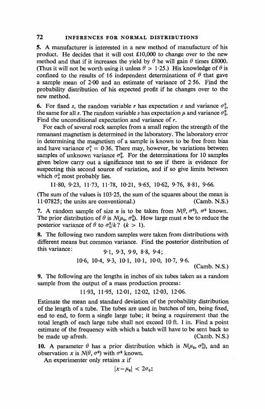
72 INFERENCES FOR NORMAL DISTRIBUTIONS
5. A manufacturer is interested in a new method of manufacture of hisproduct. He decides that it will cost £10,000 to change over to the newmethod and that if it increases the yield by 0 he will gain 0 times £8000.(Thus it will not be worth using it unless 0 > 1.25.) His knowledge of 0 isconfined to the results of 16 independent determinations of 0 that gavea sample mean of 2.00 and an estimate of variance of 2.56. Find theprobability distribution of his expected profit if he changes over to thenew method.
6. For fixed s, the random variable r has expectation s and variance o'1,the same for all s. The random variable s has expectation,u and variance o .Find the unconditional expectation and variance of r.
For each of several rock samples from a small region the strength of theremanant magnetism is determined in the laboratory. The laboratory errorin determining the magnetism of a sample is known to be free from biasand have variance o- 11L 0.36. There may, however, be variations betweensamples of unknown variance o,. For the determinations for 10 samplesgiven below carry out a significance test to see if there is evidence forsuspecting this second source of variation, and if so give limits betweenwhich o most probably lies.
11.80, 9.23, 11.73, 11.78, 10.21, 9.65, 10.62, 9.76, 8.81, 9.66.
(The sum of the values is 103.25, the sum of the squares about the mean is11.07825; the units are conventional.) (Camb. N.S.)
7. A random sample of size n is to be taken from N(0, 0.2 known.The prior distribution of 0 is N(uo, o ). How large must n be to reduce theposterior variance of 0 to (k > 1).8. The following two random samples were taken from distributions withdifferent means but common variance. Find the posterior distribution ofthis variance: 9.1, 9.3, 9.9, 8.8, 9.4;
10.6, 10.4, 9.3, 10.1, 10.1, 10.0, 10.7, 9.6.(Camb. N.S.)
9. The following are the lengths in inches of six tubes taken as a randomsample from the output of a mass production process:
11.93, 11.95, 12.01, 12.02, 12.03, 12.06.
Estimate the mean and standard deviation of the probability distributionof the length of a tube. The tubes are used in batches of ten, being fixed,end to end, to form a single large tube; it being a requirement that thetotal length of each large tube shall not exceed 10 ft. 1 in. Find a pointestimate of the frequency with which a batch will have to be sent back tobe made up afresh. (Camb. N.S.)
10. A parameter 0 has a prior distribution which is N(,uo, o ), and anobservation x is N(0, 0.2) with known.
An experimenter only retains x ifIx-i of < 2o0:
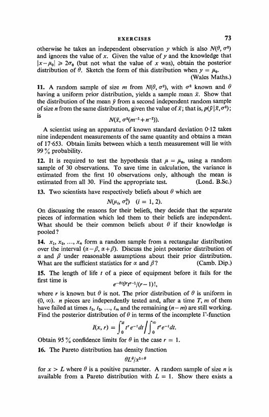
EXERCISES 73
otherwise he takes an independent observation y which is also N(O, Q2)and ignores the value of x. Given the value of y and the knowledge that1x-,uoJ >- 2o- (but not what the value of x was), obtain the posteriordistribution of 0. Sketch the form of this distribution when y = ,uo.
(Wales Maths.)
11. A random sample of size m from N(O, v2), with Q2 known and 0having a uniform prior distribution, yields a sample mean 2. Show thatthe distribution of the mean y from a second independent random sampleof size n from the same distribution, given the value of x; that is, p(y 1x,0.2);is
N(x, o2(m 1+n-1)).
A scientist using an apparatus of known standard deviation 0.12 takesnine independent measurements of the same quantity and obtains a meanof 17.653. Obtain limits between which a tenth measurement will lie with99 % probability.
12. It is required to test the hypothesis that It = ,uo, using a randomsample of 30 observations. To save time in calculation, the variance isestimated from the first 10 observations only, although the mean isestimated from all 30. Find the appropriate test. (Lond. B.Sc.)
13. Two scientists have respectively beliefs about 0 which are
N(pt, o) (i = 1, 2).On discussing the reasons for their beliefs, they decide that the separatepieces of information which led them to their beliefs are independent.What should be their common beliefs about 0 if their knowledge ispooled?
14. x1, x2, ..., x form a random sample from a rectangular distributionover the interval (a-/3, a+/3). Discuss the joint posterior distribution ofa and /3 under reasonable assumptions about their prior distribution.What are the sufficient statistics for a and /3? (Camb. Dip.)
15. The length of life t of a piece of equipment before it fails for thefirst time is e-etertr-1/(r-1)!,
where r is known but 0 is not. The prior distribution of 0 is uniform in(0, oo). n pieces are independently tested and, after a time T, m of themhave failed at times t1i t2, ..., tm and the remaining (n - m) are still working.
of 0 in terms of the incomplete F-functionFind the posterior distribution of
o1(x, r) =
f oI o tre-°dt.
Obtain 95 % confidence limits for 0 in the case r = 1.
16. The Pareto distribution has density function0LB/x1+e
for x > L where 0 is a positive parameter. A random sample of size n isavailable from a Pareto distribution with L = 1. Show there exists a
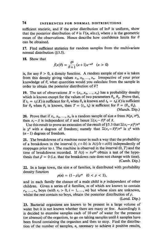
74 INFERENCES FOR NORMAL DISTRIBUTIONS
sufficient statistic, and if the prior distribution of In8 is uniform, showthat the posterior distribution of B is I'(n, nlnz), where z is the geometricmean of the observations. Hence describe how confidence limits for 0can be obtained.
17. Find sufficient statistics for random samples from the multivariatenormal distribution (§3.5).
18. Show that
f(xj0) - z
B+ 1 (x+ 1)e-:a (x > 0)
is, for any 0 > 0, a density function. A random sample of size n is takenfrom this density giving values x1, x2, ..., x". Irrespective of your priorknowledge of 0, what quantities would you calculate from the sample inorder to obtain the posterior distribution of 0?
19. The set of observations X = (xl, x2, ..., x") has a probability densitywhich is known except for the values of two parameters 0, 02. Prove that,if t1 = t,(X) is sufficient for 0, when 02 is known and t2 = t2(X) is sufficientfor 02 when 01 is known, then T = (t1, t2) is sufficient for 0 = (01, 02).
(Manch. Dip.)
20. Prove that if x1, x2, ..., x is a random sample of size n from N(,u, o'2),then xz-x is independent of x and hence E(x{-x)2 of X.
Use this result to prove an extension of the result of § 5.3 that E(x2 _/J)2/0-2is x2 with n degrees of freedom; namely that E(xt-x)2/O2 is x2 with(n- 1) degrees of freedom.
21. The breakdowns of a machine occur in such a way that the probabilityof a breakdown in the interval (t, 1+ 80 is A(t)8t+o(St) independently ofstoppages prior to t. The machine is observed in the interval (0, T) and thetime of breakdowns recorded. If ll(t) = ae$t obtain a test of the hypo-thesis that /3 = 0 (i.e. that the breakdown rate does not change with time).
(Camb. Dip.)
22. In a large town, the size n of families, is distributed with probabilitydensity function
p(n)=(1-p)p" (0<p<1),and in each family the chance of a male child is p independent of otherchildren. Given a series of k families, m of which are known to containr1, ..., rm boys (with r{ > 0, i = 1, ..., m) but whose sizes are unknown,whilst the rest contain no boys, obtain the posterior distribution of p.
(Lond. Dip.)
23. Bacterial organisms are known to be present in a large volume ofwater but it is not known whether there are many or few. Accordingly itis decided to examine samples each of 10 cm3 of water for the presence(or absence) of the organism, to go on taking samples until k samples havebeen found containing the organism and then to stop. Find the distribu-tion of the number of samples, n, necessary to achieve k positive results,
EXERCISES 75
and the mean and standard deviation of this distribution. Explain how toset up confidence limits for p, the proportion of infected samples, so thatone may be 100a % certain that p will lie within these limits.
(Lond. Dip.)
24. A Geiger counter has a probability OBu+ O(6u2) of clicking during thetime interval u, u+Su, independent of u and all previous clicks.
If the average interval between consecutive members of a sequence of11 clicks is 2.2 sec, show that 0 may be asserted to lie in the range0.25 (sec)-1 to 0.71 (sec)-1 with a 90 % level of confidence. (Camb. N.S.)
25. Certain radioactive substances emit particles at random at an averagerate A. n intervals between such emissions are observed for each of twosuch substances, the mean intervals being x and y respectively. Explainhow you could test whether the rates of emission are the same.
(Leic. Gen.)
26. Observations are made as follows on a Poisson process in whichevents occur at unknown rate 0 per unit time. In the time period (0, u] itis observed that m events occur at instants x1 < x2 < ... < x,,,, whereasin the time interval (u, 2u] it is observed only that n events occur, theinstants of occurrence not being recorded. What is the (minimal) sufficientstatistic for 0 and what is its sampling distribution? (Lond. M.Sc.)
76
6
INFERENCES FOR SEVERAL NORMALDISTRIBUTIONS
The previous chapter was concerned with the problems ofinference that arise when a single sample is taken from a normaldistribution: in this chapter similar problems are consideredwhen two or more samples are taken from possibly differentnormal distributions. We shall continue to use uniform priordistributions for the mean and the logarithm of the variance,thinking of them as approximations to distributions representinglittle prior knowledge of the parameters, as in theorem 5.2.1.
6.1. Comparison of two means
Theorem 1. Let x1 = (x11, x12, ..., xln.) be a random sample ofsize n1 from N(01, 0.1) and x2 = (x21, x22, ..., x2n,) be an inde-pendent random sample of size n2 from N(02i v2), where a-1 and O2are known. Then if the prior distributions of 0 and B2 are indepen-dent and both uniform over (- oo, oo), the posterior distribution of8 = 01- 02 is N(21- x2, (711n1 + O'2/n2), where xl and x2 are therespective means of the two samples.
The joint prior distribution of 0 and 02 is everywhere con-stant and the likelihood of the two samples is (equation 5.1.9)proportional to
C -expn1(x1- B1)2 n2(x2 -
02)2( )20.1 20.2 1
so that (1) is also proportional to the joint posterior distributionof 0 and 02 given x1 and x2. This is a product of two factors,one involving 0 only, one involving 02 only, and hence (§3.1)91 and 02 are independent. Furthermore, they are clearlyN(x1i 0,11n) and N(x2, v2/n2) respectively. This could bededuced directly from the corollary to theorem 5.1.1 witho-o - co.) Since, if 02 is normal so is - 02, it follows fromtheorem 3.5.5 that 6 = 01- 02 is also normal with mean equal
6.11 COMPARISON OF TWO MEANS 77
to the difference of the means and variance equal to the sum ofthe variances.
Theorem 2. Let x1 be a random sample of size n1 from N(01, 0)and x2 be an independent random sample of size n2 from N(021 0).Then if the prior distributions of 01, 02 and In 0 are independent anduniform over (- oo, oo), the posterior distribution of vs2/0 is X2with v degrees of freedom, where
n;/ ( 1visa = Sa = (.xj -xg)2, vi = n=- 1 (i = 1, 2) (2)
j=1
and vs2 = S2 = S1 + S2, v = v1 + v2. (3)
[Note that the variances of the two normal distributions fromwhich samples are taken are supposedly known to be equal.]
The joint prior density of 01i 02 and 0 is proportional to 0-1and the likelihoods of the two samples are given by equation5.4.3 (with the change of a few suffixes to distinguish the twosamples). The likelihoods may be rearranged in the form (5.4.4)and multiplying these expressions together we see that the jointposterior distribution of 01, 02 and 0 is
n (01, 02, 01 x1, x2) oC c-1(ni+n2+2) exp [ - {n1(x1- 01)2
+ n2(22 - 02)2 + S2 + S2}/20] (4)
To obtain the posterior distribution of 0 it is only necessary tointegrate (4) with respect to 81 and 02. This is easily done sincethe two integrals are the usual normal ones (compare the passageto equation 5.4.6) and the result is
7T(o I x1, x2) cc e-v8'/20 q5-1v-1 (5)
A comparison with equation 5.3.2 establishes the result.
Theorem 3. Under the same conditions as in theorem 2 theposterior distribution of 8 = 01- 02 is such that
t = {(2 - x2) - 8}/s{l /n1 + 1 /n2} (6)
has Student's t-distribution with v degrees of freedom.The situations in theorem 3 and in theorem 1 (with v1 = °2)
are the same except that 0, unknown in theorem 3, is known in
78 INFERENCES FOR SEVERAL DISTRIBUTIONS [6.1
theorem 1 to be equal to the common value of o'1 and o'2. Hencetheorem 1, in the notation of this theorem, says that
ii(8I c, xl, x2) is N(21-2, 0{l /n1 + 1 /n2})
Furthermore, 7r(g I x1, x2) is known from theorem 2, so com-bining these results we have
n(8,Y 1 x1, x2)
IT(8I 0, x1, x2) 7T(o I x1, x2)
1cC r -J(v+3)exp [-((I +n21) [8- (xl-x2)]2+VS2)/20
_ 0-t(v+3)eXp[-(t2/V+1) Vs2/2c], (7)
on substituting the expression (6) for t. The integration withrespect to 0 is easily carried out using theorem 5.3.2 with theresult that
10 I x1, x2) cc {1 + t2/v}-Icv+1> (8)
The Jacobian of the transformation from 8 to t is a constant sothat a comparison with equation 5.4.1 establishes the result.
A few definitions will be useful. S2 is called the sum ofsquares, vl the degrees of freedom and si = S2/v1 the meansquare, for the first sample; with similar definitions for thesecond sample. S2 is called the within sum of squares and v thewithin degrees of freedom. s2 = S21v is the mean square for .These terms will be used again later (§6.5).
Comparative experimentsComparative experiments, in which several samples are com-
pared, are much more common than single sample experimentsin which the comparison is with some standard. For example,a scientist wishing to investigate the qualities of a new variety ofwheat would not merely sow some fields with it and obtainyields, the liability to disease and other factors, since he mightobtain a good yield because it was a good year and freedomfrom disease because it was generally a disease-free year. Hewould sow neighbouring fields, or plots, some with the newvariety and some with one or more varieties which had beenused for several years and whose behaviour was well known.
6.1] COMPARISON OF TWO MEANS 79
The new variety would be judged by comparison with the olderones: he is using what scientists call a control. This is a compara-tive experiment with two or more samples. The experiments usedto illustrate the single sample techniques in chapter 5 were allabsolute experiments (to measure the conductivity of thematerial (§5.1)) or experiments to compare new material witha standard (to compare the precision of a new instrument withthe standard (§ 5.3)). In some branches of science standards arenot easy to obtain and it is necessary to use controls. Evenwhere standards are available a comparative experiment may bepreferable because the error is less: a point to be discussed indetail under paired comparisons below.
Case of known variancesTheorem 1 is the simplest case of a two-sample experiment
and is a direct extension of the corresponding result for thesingle-sample experiment (theorem 5.2.1). The variances of thetwo normal distributions are supposed known and the twosamples are independent. It is clear from the likelihood (1) thatthe two sample means are jointly sufficient for the populationmeans. The joint posterior distribution of 01 and 02 is normalwith means xl and x2 and variances i/n1 and v2/n2i and, sincethey are independent, correlation zero. It is usually, however,just the difference 8 = 01- 02 that is of interest, and theorem3.5.5 shows that it is also normally distributed. Consequentlyconfidence intervals for it may be constructed in exactly thesame way as with the single value 01. Thus with 7-2 = al/n1 + 0-2/n2,the posterior variance of 8, a 95 % confidence interval for 8 is(xl - x2) ± 1.96r. It is quite usual for the value 6 = 8 = 0 to beof especial interest because it corresponds to the two meansbeing equal. For example, if the first sample is taken from thenew material and the second from the control, the null hypo-thesis 6 = 0 would say that the mean of the new material wasthe same as that of the control, whereas if it were not zero thenthere would be some difference between them. The result will besignificant at the 5 % level if 1x1 - x2 IT exceeds 1.96. If it is onlyof interest to know whether the new material is an improvementover the control, in the sense of having higher mean, then only
80 INFERENCES FOR SEVERAL DISTRIBUTIONS [6.1
values of 8 > 0 are of interest and a one-sided confidenceinterval would be used leading to a different significance test.Thus, we would be fairly certain that 8 > (z1- z2) - 2.33T, usinga 99 % confidence interval [(D(2-33) = 0.99] and the result wouldbe judged significant at the 1 % level if this interval does notinclude 8 = 0, that is, if (z1 - z2)1T > 2.33. But a significancetest is rarely adequate in this situation because if the result issignificant (that is, you feel fairly sure that the new materialis better than the control) then you naturally want to knowhow much better. Even if it is not significant the additionalknowledge of the confidence interval is valuable because itprovides a warning of what values of 8, apart from zero, arereasonable. If the confidence interval is too wide you may feelobliged to take additional measurements before being contentthat the new material is not different from the control. We againissue the warning that a significance test is not a method ofmaking decisions : it only expresses one's degree of belief aboutthe null hypothesis. If the scientist has to decide whether or notto grow the new variety he should use the methods of decisiontheory, as explained in § 5.6. Similarly, if he has prior reason tobelieve that 8 is 0, or is very near zero, this prior informationshould be incorporated into the analysis. For example, if 0l and02 have a joint prior normal distribution which is such that8 = 01-02 has mean zero and small variance, theorem 6.6.3may be used to obtain a posterior normal distribution for 8 thatincorporates this prior knowledge.
Case of unknown varianceTheorem 3 is an extension of theorem 1 to the case where the
variances are unknown and is similar to the extension of thesingle sample case with variance known (theorem 5.2.1) to thecase of unknown variance (theorem 5.4.1). In both extensionsthe normal distribution is replaced by the t-distribution butotherwise the methods are the same. Theorem 2 is also similar tothe single sample variance result (theorem 5.4.2) leading againto a X2-distribution. But before discussing the simplicity andelegance of these extensions it must be emphasized that in boththeorems it is assumed that the two normal distributions have
6.11 COMPARISON OF TWO MEANS 81
the same variance, even though the common value is unknown.This severe assumption is often likely to be satisfied in practicalapplications. For example, the same measuring instrument maybe used in both samples, giving the same precision; or the vari-ability in the two samples may be due to common causes, aswith wheat, where it is unlikely that the two varieties woulddiffer in their variability over a field. j' The corresponding resultwhere the variances are not assumed equal will be given in §6.3,and will show that there is not much difference between the twosituations (variances equal or unequal) as far as the differenceof means is concerned. The elegance and simplicity of the resultswhen the variances are equal, the beautiful extensions to severalsamples (§6.4) and the analysis of variance (§6.5), make theassumption a most convenient one.
We discuss theorem 3 first. In the case of known, equalvariances, o-i = 62 = o-2, theorem 1 says that
{(2 - x2) - 6}/0-{1 In, + 1 /n2}1 (9)
has a posterior distribution N(0, 1). The quantity t, equation (6),is the same as (9) except that s replaces o-. So we have a paral-lelism between the two situations closely similar to that existingin the single sample case, 5.4(i) and (ii). Confidence intervalsand significance tests for 6 = 0 may be constructed in the sameway as for known o, with the substitution of s for o- andStudent's distribution for the normal. These are the samereplacements as were needed in passing from 5.4(i) to (ii) andneed not be discussed again. What do merit attention, however,are the values of s and v, the degrees of freedom for t. There aretwo sources for the posterior knowledge of the variance; namelythe two samples. In § 5.4 we saw that the sum of squares of thesample values about their mean divided by the number of ob-servations, n, was a reasonable statistic to replace the variance.In fact we divided by (n - 1) for a reason which will appear ina moment. Similarly, in the two sample case S2/v1 = si andS22/V2 = s2 are both reasonable estimates of the variance and we
t With wheat, it is usually the coefficient of variation that stays constant; butif the means do not differ too much the variances will not either.
6 LS it
82 INFERENCES FOR SEVERAL DISTRIBUTIONS [6.1
naturally combine them. A suggestion would be to take theiraverage i (si + s2) but the analysis of the theorem shows that theweighted average (vlsi+v2s2)/(v1+v2) = s2 is the more con-venient quantity to use because, from equation (4), s2, z1 and x2are jointly sufficient. So what we do (in terms of the definitionsabove) is to take the sums of squares for the two samples andadd them together obtaining the within sum of squares; to takethe degrees of freedom for the two samples and add themtogether obtaining the within degrees of freedom; and divide theformer by the latter to obtain the mean square to replace thevariance. This simple procedure of addition of sums of squaresand degrees of freedom generalizes to more complicated situa-tions. (Notice that the sums of squares are always sums ofsquares about the sample means; the last four words are under-stood in speaking of sums of squares. Sums of squares aboutthe origin are called uncorrected (§6.5).)
We can now explain the term `degrees of freedom'. The sum
S1 = E (x1i - x&z=1
is the sum of the squares of n1 terms and therefore appears atfirst glance to have n1 parts which can vary. But the terms areconstrained (to use a mechanical term) to add to zero, since
n,(x1d - x) = 0, so that once values are assigned to (n1-1) of
4=1
them, the last is then fixed. To continue the analogy withmechanics, it is rather like a mechanical system of n1 parts withonly (n1-1) of them free to vary because of a single constraint,and we say, as we would of the mechanical system, that it has(n1-1) degrees of freedom. Similarly, S2 has (n2- 1) degrees offreedom and S2, the sum of n1+n2 terms with two constraintshas n1 + n2 - 2 = (n1-1) + (n2- 1) degrees of freedom. Againthis idea extends to more complicated situations. The exten-sion will also explain the use of the adjective `within'.
It is also possible to see (at the cost of a little algebra which isomitted) why the degrees of freedom were used to divide the sumof squares, and not n. Suppose s*2 = E(x. - x)2/n had been usedin § 5.4 instead of s2 and t* had been defined as t with s* for s.
6.11 COMPARISON OF TWO MEANS 83
Then the posterior distribution of t* would have been pro-portional to (1 + t*2/n)-In. (10)
If, in the two-sample case, s*2 = (Si + S2)/(n1 + n2) had beenused instead of s2 then the posterior distribution of t*, definedas t with s* for s, would have been proportional to
{l + t*2/(nl + n2)}--Y%+n2-1). (11)
Now (10) and (11) are not of the same form, with n1+n2replacing n, and new tables would be needed for the situation ofthis section: whereas (8) is the same as expression 5.4.1, andthe same tables suffice.
An alternative proof of theorem 3 starts from equation (4).In this we can change variables to S = 01- 02 and 01 + 02, say,and integrate with respect to 01+02 to obtain (7), the jointdensity of S and 0. The argument using conditional probabilitiesavoids this integration, or rather utilizes the fact that it hasalready been done in the proof of theorem 1, in effect.
Theorem 2 is a natural extension of theorem 5.4.2. Thedegrees of freedom still determine which X2-distribution isappropriate and the quantity which, when divided by the vari-ance, has this distribution is still the sum of squares, vs2, herethe total sum of squares. Inferences about the variance cantherefore be made using the X2-distribution in exactly the sameway as for a single sample.
Paired comparisonsWhenever a theorem is used one should make sure that the
conditions of the theorem are reasonably well satisfied. This isparticularly true of theorems 1 and 3, and we now illustratea possible misuse of them. As we have already explaineda common use of the result is in experiments that compare acontrol and a new treatment. One way of designing such experi-ments can be illustrated on a method used to examine the effectof a paint in preventing corrosion. Pieces of metal had one halftreated with the paint and the other left in the usual stateappropriate to the use that the metal was to be put. The pieceswere placed in a wide range of positions, differing in exposure
6-z
84 INFERENCES FOR SEVERAL DISTRIBUTIONS [6.1
to weather, etc., and at the end of a suitable period of timemeasurements were made of the corrosion, x1i, on the untreatedpart and also, x22, on the treated part of the ith piece. It is notunreasonable to suppose that the x1i form a random samplefrom N(01, ¢) where 01 is the average corrosion and ¢ is ameasure of the variability under different conditions of expo-sure, etc. Similarly, the x2i form a random sample fromN(02, 0), assuming the same variability for painted and un-painted metal. We wish to investigate B1- 02, the average reduc-tion in corrosion due to painting. At first glance it would appearthat theorem 3 could be used, but this is not so because the tworandom samples {xli} and {x2i} are not independent. Since x1iand x2i refer to the corrosion on two parts of a piece of metalsubject to identical conditions except for the painting, they arelikely to be much closer together than, say, x1i and x25 (j* i)which were in different conditions of exposure. Consequentlythe conditions of the theorem are not satisfied and the likelihoodwould be different because of the correlations between x1a and x2i.
Inferences about 01- 02 may be made in the following way.The random variables zi = x1,- x2i have expectations 01- 02and variances 01, say, and might perhaps be assumed normallydistributed. (If x1i and x2i have a bivariate normal distributionthis will follow from theorem 3.5.5.) If so they would form arandom sample from a normal distribution, since the separatepieces of metal are probably independent, and we would wishto make inferences about the mean of this distribution. This isa single sample problem and theorem 5.4.1 enables the usualconfidence limits, or significance test for the mean being zero, tobe found with the aid of the t-distribution. Notice that thisanalysis does not assume that x1i and x2i have the samevariances.
Although this method is valid, it is not obvious that it isa complete inference about 01-02 from the whole of the data.The argument amounts to considering only the differencesbetween the two values on the same plate and takes no accountof the separate values. Although it is intuitively obvious thatno information about 01- 02 is lost by this procedure theargument does need further justification.
6.1] COMPARISON OF TWO MEANS 85
This is provided by remarking that we can write, withwi = x1, + x2i, omitting reference to the parameters, and the restof the notation obvious,
P(X1, X2) = P(z, W) = P(z)P(w I z)
Whilst p(z) depends on 8, p(w I z) typically will not, and, what-ever parameters the latter does depend on, they will usually notoccur in p(z) and will, prior to the observations, be independentof those in p(z). Consequently as far as inferences about 8 areconcerned we may confine attention to p(z), absorbing p(w j z)into the constant of proportionality. (Compare the discussionon ancillary statistics in § 5.5.) If x1i and x2i, and hence zi andwi, have a bivariate normal distribution, wi, for fixed z,, willdepend on a, ,8, 0-2 (equations 3.2.13 and 3.2.14) whilst zi willdepend on ,u1 and 0-1 (in the notation of §3.2). ,a1 is here 8, andprovided (a, 8, o.2) and (It,, vi) are independent the inferenceusing z only will not lose any information.
Two practical points of interest emerge from the experiment.First, the quantity 01 - 02, whose posterior distribution, giventhe observed differences, has been found, is the average reduc-tion over the conditions of the experiment, and may not be themost sensible thing to consider. For example, suppose the effectof the paint is to reduce the corrosion by a fixed percentageirrespective of the amount of the corrosion. Then 02 = A61 andthe difference is 61(1-A). But 61 may be different if the experi-ment is done again and is, in any case, irrelevant in assessing theeffect of the paint. The quantity of interest is A and this may bestudied by taking logarithms of the readings: the differences ofthese will have an approximate mean value of In A and inferencescan be made about that, although it must be remembered thatthe logarithms might not have a normal distribution. It isimportant, in applications, to make sure that one is applying thetheoretical results to the quantity of interest.
Secondly, one might ask why this experimental design wasused at all. Why not take a random sample of painted pieces anda second, independent, random sample of unpainted pieces ?The reason is that the precision of the determination of theeffect, whether measured by the inverse of the variance of the
86 INFERENCES FOR SEVERAL DISTRIBUTIONS [6.1
posterior distribution or by some other means, such as consider-ing the width of the final confidence interval, depends on thetrue variance of the normal distribution (or distributions) fromwhich the samples have been taken. The x1i and the x2i will havea variance which includes the variation from place to placewhereas the differences x1i - x21 will have a variance, which onlyinvolves variations due to the instrument measuring the cor-rosion and to any minor differences in the two parts of the samepiece of metal. Consequently the effect of taking the differencesis to reduce, probably very considerably, the variance, and henceincrease the precision of the determination of the effect ofpainting. As the readings are taken in pairs the method istermed `paired comparisons'. We shall later (§§6.4, 6.5) see howto extend this idea and to analyse the variability in some experi-ments into different parts in order to remove the larger parts andpermit a more sensitive analysis.
6.2. Comparison of two variancesIf a random variable, usually in this context denoted by F,
has a density proportional to
Five-1/(v2 + v1F)Ic°1+v-) (1)
for F > 0, and zero otherwise, where v1 and v2 are positive, it issaid to have Fisher's f F-distribution with vl and v2 degrees of
freedom, or simply an F-distribution. We shall often speak of anF(v1, v2) distribution. Notice that the order of reference to thedegrees of freedom is relevant: F(v1, v2) is not the same asF(v2, v1)Theorem 1. Let xi = (xi1, xi2, ..., xi,t) be a random sample ofsize ni from N(0i, 0i) (i = 1, 2), with x1 and x2 independent; letthe prior distributions of 01, 02, In q1 and In 02 be independent andeach uniform over (- oo, oo). Then the posterior distribution of(Si/s2)/(c1/Cb2) is F(v1, v2), where 91, s2, v1 and v2 are as in theorem6.1.2.
Because of the independence, both of the samples and of theprior distributions, the posterior distributions of 01 and 02 areindependents and their separate distributions are given by
t Some writers refer to it as Snedecor's F-distribution.$ Compare the argument with which the proof of theorem 6.1.1 began.
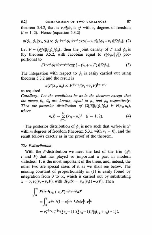
6.21 COMPARISON OF TWO VARIANCES 87
theorem 5.4.2, that is vis2/y'i is x2 with vi degrees of freedom(i = 1, 2). Hence (equation 5.3.2)
1T01, 021 X1, X2) cc 01 2 Iva-lexp{- v1si/2b1- V2S2/2q52} (2)
Let F = (si/s2)/(c1/02); then the joint density of F and 02 is(by theorem 3.5.2, with Jacobian equal to si02/s202 pro-portional to
Fiv1-102 Yv1+v2)-1 exp { - (v2 + vl F) s2/202} (3)
The integration with respect to 02 is easily carried out usingtheorem 5.3.2 and the result is
ir(FI x1, x2) oc FIv1-1/(v2 + v1 F)I(v1+v2)
as required.Corollary. Let the conditions be as in the theorem except thatthe means 01, 02 are known, equal to ,ul and ,u2 respectively.Then the posterior distribution of (si/ 2)/\O1/O2) is F(n1, n2),where
n;
(1 = 1, 2). (4)12Sti = (xif -lui)2j=1
The posterior distribution of 01 is now such that ni3i/oi is x2with ni degrees of freedom (theorem 5.3.1 with vo = 0), and theresult follows exactly as in the proof of the theorem.
The F-distributionWith the F-distribution we meet the last of the trio (x2,
t and F) that has played so important a part in modernstatistics. It is the most important of the three, and, indeed, theother two are special cases of it as we shall see below. Themissing constant of proportionality in (1) is easily found byintegration from 0 to co, which is carried out by substitutingx = v1 F/(v2 + v1 F), with dF/dx = v2/ [vl(1- x)2]. Then
FIv1-1(V2 + vl F)-I(vl+va)dF0J -rl
J xlvl-1(1-x)Iva-ldx/vlvlvjva0
= V1 Iv1V2 Iv2(1V1- 1)! (.-V2- 1)!/[2(V1+ V2)- 1!.
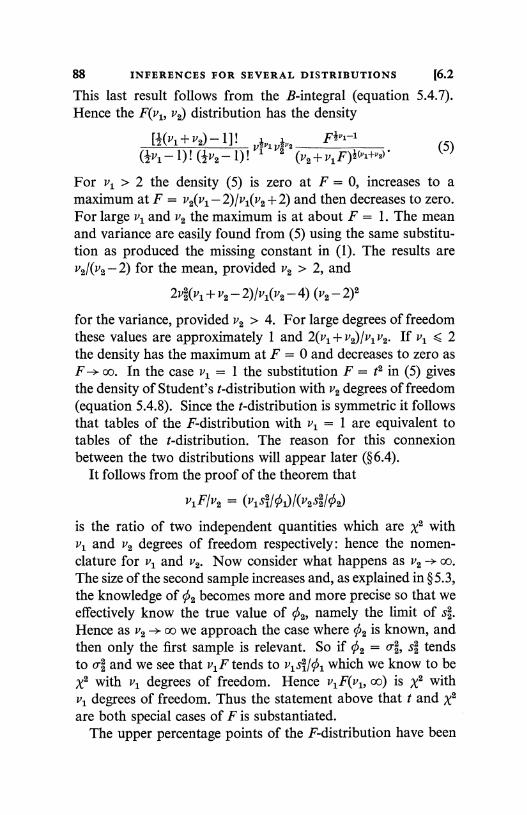
88 INFERENCES FOR SEVERAL DISTRIBUTIONS [6.2
This last result follows from the B-integral (equation 5.4.7).Hence the F(v1, v2) distribution has the density
5vv(v1-1)!(±P2-1)! (v2 + v1 F)I(°i+"2)
For v1 > 2 the density (5) is zero at F = 0, increases to amaximum at F = v2(v1- 2)/v1(v2 + 2) and then decreases to zero.For large v1 and v2 the maximum is at about F = 1. The meanand variance are easily found from (5) using the same substitu-tion as produced the missing constant in (1). The results arev2/(v2 - 2) for the mean, provided/ v2 > 2, and
2v2(v1 + v2 - 2)/v1(v2 -4) (v2 - 2)2
for the variance, provided v2 > 4. For large degrees of freedomthese values are approximately 1 and 2(v1 + v2)/v1 v2. If v1 5 2the density has the maximum at F = 0 and decreases to zero asF --> co. In the case vi = 1 the substitution F = t2 in (5) givesthe density of Student's t-distribution with v2 degrees of freedom(equation 5.4.8). Since the t-distribution is symmetric it followsthat tables of the F-distribution with vi = 1 are equivalent totables of the t-distribution. The reason for this connexionbetween the two distributions will appear later (§6.4).
It follows from the proof of the theorem that
v1F/v2 = (v1s1/cb10(v2s2/cb2)
is the ratio of two independent quantities which are x2 withvi and v2 degrees of freedom respectively: hence the nomen-clature for v1 and v2. Now consider what happens as v2 -- 00-The size of the second sample increases and, as explained in § 5.3,the knowledge of 02 becomes more and more precise so that weeffectively know the true value of ¢2, namely the limit of s2.Hence as v2 -> 00 we approach the case where 02 is known, andthen only the first sample is relevant. So if 02 = 02i s2 tendsto 02 and we see that v1F tends to vlsl/0i which we know to bex2 with v1 degrees of freedom. Hence v1F(vl, oo) is x2 withv1 degrees of freedom. Thus the statement above that t and x2are both special cases of F is substantiated.
The upper percentage points of the F-distribution have been
I "2F'ivi-i[(yi + y2) - 1 J I
l vi
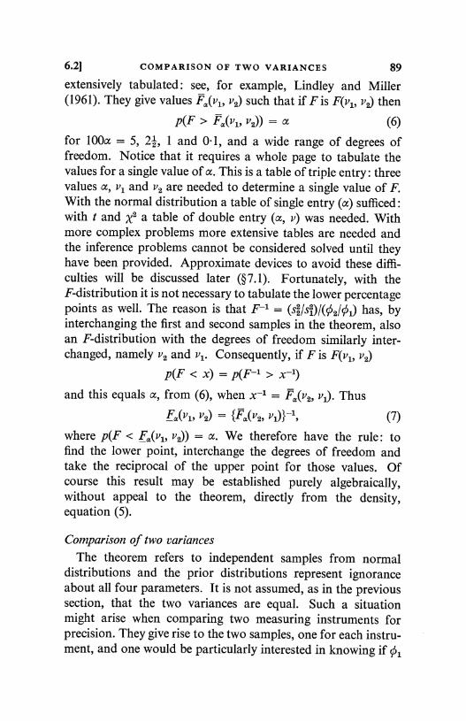
6.2] COMPARISON OF TWO VARIANCES 89
extensively tabulated : see, for example, Lindley and Miller(1961). They give values F,,(P,, v2) such that if F is F(v1, v2) then
p(F > Fa(v1, v2)) = a (6)
for 100a = 5, 22, 1 and 0.1, and a wide range of degrees offreedom. Notice that it requires a whole page to tabulate thevalues for a single value of a. This is a table of triple entry: threevalues a, vl and v2 are needed to determine a single value of F.With the normal distribution a table of single entry (a) sufficed:with t and x2 a table of double entry (a, v) was needed. Withmore complex problems more extensive tables are needed andthe inference problems cannot be considered solved until theyhave been provided. Approximate devices to avoid these diffi-culties will be discussed later (§7.1). Fortunately, with theF-distribution it is not necessary to tabulate the lower percentagepoints as well. The reason is that F-1 = (s2/s12)has, byinterchanging the first and second samples in the theorem, alsoan F-distribution with the degrees of freedom similarly inter-changed, namely v2 and v1. Consequently, if F is F(v1, v2)
p(F < x) = p(F-1 > x-1)
and this equals a, from (6), when x-1 = Fa(v2, vi)- Thus
Fa(vl, v2) = {Fa(v2, v1)}-1, (7)
where p(F < Fa(vl, v2)) = a. We therefore have the rule: tofind the lower point, interchange the degrees of freedom andtake the reciprocal of the upper point for those values. Ofcourse this result may be established purely algebraically,without appeal to the theorem, directly from the density,equation (5).
Comparison of two variances
The theorem refers to independent samples from normaldistributions and the prior distributions represent ignoranceabout all four parameters. It is not assumed, as in the previoussection, that the two variances are equal. Such a situationmight arise when comparing two measuring instruments forprecision. They give rise to the two samples, one for each instru-ment, and one would be particularly interested in knowing if c1
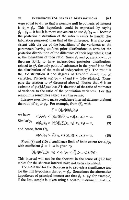
90 INFERENCES FOR SEVERAL DISTRIBUTIONS [6.2
were equal to q2, so that a possible null hypothesis of interestis 01 = 02. This hypothesis could be expressed by sayingY'1- 02 = 0 but it is more convenient to use 01/02 = 1 becausethe posterior distribution of the ratio is easier to handle (fortabulation purposes) than that of the difference. It is also con-sistent with the use of the logarithms of the variances as theparameters having uniform prior distributions to consider theposterior distribution of the difference of their logarithms; thatis, the logarithms of their ratio. Since 01 and 02 are known, bytheorem 5.4.2, to have independent posterior distributionsrelated to x2, the only point of substance in the proof is to findthe distribution of the ratio of independent x2's. The result isthe F-distribution if the degrees of freedom divide the x2variables. Precisely, vas?/0ti = xi and F = (x1/v1)/(x2/v2). (Com-pare the relation to x2 discussed above.) Notice that sz is anestimate of OY (§ 5.3) so that F is the ratio of the ratio of estimatesof variance to the ratio of the population variances. For thisreason it is sometimes called a variance-ratio.
It is now possible to make confidence interval statements aboutthe ratio of ¢1 to 02. For example, from (6), with
F = (s1/s2)/(01/02)
we have(sl/S2/Fa(v1, V2)1 X1, X2) = Z. (8)
Similarly,7T(01102 > (s1/s2)/Fa(r1, V2)1 x1, X2) = a, (9)
and hence, from (7),
701/02 > Fa(v2, PO (411s2) I X1, X2) = a. (10)
From (8) and (10) a confidence limit of finite extent for Y.1/02with coefficient /3 = 1-a is given by
S211S
2)/FIa(vl, v2) < 01/02 < FIa(v2, vl) (s1/s2).
This interval will not be the shortest in the sense of § 5.2 buttables for the shortest interval have not been calculated.
The main use for the theorem is to provide a significance testfor the null hypothesis that 01 = 02. Sometimes the alternativehypotheses of principal interest are that 01 > 02: for example,if the first sample is taken using a control instrument, and the
6.21 COMPARISON OF TWO VARIANCES 91
second using a new instrument, one may only be interested inthe latter if it is more accurate. The confidence limit requiredwould be that c51/c52 exceeds some value, so would be obtainedfrom (8). The result would be significant if the confidenceinterval did not contain the value 1. That is, if the interval in (8)did contain this value. Hence it //is significant at the level (a if
S1/S2 > F (vl, v2) (11)
The final inequality is simply that the ratio of the samplevariances exceeds the upper 100a % point of the F-distributionwith vl and v2 degrees of freedom: the first degree of freedomrefers to the numerator of the sample ratio. This one-sidedsignificance test will appear again later (§6.4) in an importantproblem.
The corollary is not often useful since it is unusual for themeans to be known but not the variances. There is little need tocomment on it except to remark that we again have the F-distribution, and the only difference is that the degrees offreedom are equal to the sample sizes and not one less thanthem. Otherwise confidence intervals and significance tests areas before.
6.3. General comparison of two meansIf tl and t2 are independent random variables each distributed
in Student's t-distribution, with vl and v2 degrees of freedomrespectively, and if W is a constant, representing an anglebetween 0 and 90 degrees, the random variable
d = t1coslil-t2sin6) (1)
will be said to have Behrens's distribution with vl and v2 degreesof freedom and angle Co.
Theorem 1. Let the conditions be the same as those of theorem6.2.1; then the posterior distribution of S =0,-02 is such that/
d = {S - (2 - z2)I/(Si/nl + s2/n2)* (2)
has Behrens's distribution with vl and v2 degrees of freedom, andangle co given by
tan W = (s2/Vn2)/(s1/V n). (3)
92 INFERENCES FOR SEVERAL DISTRIBUTIONS [6.3
Again, because of the independence both of the samples andof the prior distributions, the posterior distributions of 0, and02 are independent and their separate distributions are given bytheorem 5.4.1. That is, n ( 0 i - 2)/s8 = ti, say, has Student'st-distribution with v, degrees of freedom (i = 1, 2). We have
BE - xi = tz sil Jn= (i = 1, 2)/so that (01- 02) - (2 - x2) = t1(s1 /V nl) - t2(s2l'V n2),
or, dividing by (si/n1+s2/n2)1 and using (2) and (3),
d = tlcosW-t2sin&l,
which, on comparison with (1), proves the theorem.
Behrens's distributionWe shall not attempt any detailed study of Behrens's
distribution. It will suffice to remark that it is symmetricalabout d = 0, that its moments follow easily from those ofStudent's distribution and that, as v1 and v2 both tend toinfinity it tends to normality. This final result follows becausethe t-distribution tends to normality (§ 5.4) and the difference ofnormal variables is also normal (theorem 3.5.5). Some per-centage points of the distribution are to be found in Fisherand Yates (1963). These tables give values da(vl, v2, suchthat
')I x1, X2) = a7r(I d I > dl(v1, v2, c (4)
and because of the symmetry
7r(d > da(v1, v2, @)I Xl, X2) = a. (5)
Comparison of two meansTheorem 1 differs from theorem 6.1.3 only that in the latter
the two variances are assumed equal with a uniform prior distri-bution for the logarithm of their common value, whereas herethe two variances are supposed independent with each logarithmuniformly distributed. In both situations we seek the posteriordistribution of the differences between the means, 01- 02 = s.We recall that in using the earlier theorem the two estimates of
6.3] GENERAL COMPARISON OF TWO MEANS 93
variance, sl and s2, from the two samples were pooled to providea single estimate s2 given by vs2 = v1si+v2s2 with v = v1+v2.The quantity t was then obtained by taking the quantity usedwhen the common variance, o.2, was known (equation 6.1.9) andreplacing o in it by the estimate s. In the present situation thetwo variances must be separately estimated, by s; and 92, andthe quantity used when the variances are known
{8 - (2 - x2)}/(ej/n1 + o'2/n2)I
(from theorem 6.1.1 where it is shown to be N(0, 1)) continuesto be used, but with S2 and s2 replacing 0-1 and 02: this gives (2).Unfortunately its distribution is complicated, and furthermoredepends on three parameters, so that a table of quadruple entryis needed. The change of the percentage points with w, and withv1 and v2 when these are both large, is small so that rather coarsegrouping of the arguments is possible in tabulation. Notice thatthe statistic d is still (see § 5.4) of the form : the differencebetween 8 (the unknown value) and the difference of samplemeans, divided by the estimated standard deviation of this differ-ence. For _q2(Xi - x2) = 0-21/n1 + 02/n2i since the samples, andhence xi and x2, are independent. Confidence limits for 6 aretherefore provided in the usual way by taking the sample differ-ence plus or minus a multiple, depending on Behrens's dis-tribution, of the estimated standard deviation of this differ-ence. Thus, from (4), writing da for da(v1, v2, W),
7!(21- x2 - dl.(sl/n1 + S2/n2)I
5 8 Xi - x2 + dda(S2/n1 + S2/n2)11 X1, X2) = /3A (6)
where, as usual, a = 1- f. A significance test of 8 = 0 atlevel a is obtained by declaring the result to be significant if thisinterval does not contain the origin.
Relationship to Student's problemIt is a moot point which of theorems 6.1.3 and the present one
should be used in practical problems. Fortunately the differ-ences are not very great; that is ta(v1 + v2) is not usually verydifferent from da(v1, v2, G,), and the differences between poolingthe variances or using them separately are usually small, at least
94 INFERENCES FOR SEVERAL DISTRIBUTIONS [6.3
if the sample sizes are nearly equal. Another argument that issometimes used is the following. In an obvious abbreviatednotation the joint posterior distribution of a and O1/O2 may bewritten
7i(8, 011021 x) = ii(sl 01/02, x) 701/Y'21 X) (7)
Now rr(01/021 x) is known (theorem 6.2.1). Suppose that thishas its maximum value near c1/cb2 = 1 and that it decreasessharply from the maximum : in other words, a confidenceinterval for 01/¢2 is a small interval containing 1. Then anintegration of (7) with respect to 01/02i in order to obtain themarginal distribution of 6, will only have an appreciable inte-grand near 01/02 = 1 and will therefore be approximatelynr(Sl 1, x) which gives Student's distribution (theorem 6.1.3).Consequently, one can first investigate the ratio of variancesand, if this suggests that they are about equal, use Student'smethod based on the assumption that they are. The adequacyof the approximation has not been investigated. Often it is heldenough that the test for 01/02 = 1 be not significant for Student'smethod to be used: that is, one merely looks to see if the confi-dence interval contains 1, not how small it is. There seems littlepoint in doing this here since Behrens's distribution is tabu-lated, but in more complicated situations the procedure of usinga preliminary significance test has much to recommend it (see§6.5). Undoubtedly the simplicity and elegant extensions(§§6.4, 8.3) of the equal variances result make it more attractivein practical situations and it is used today far more often thanBehrens's result. There is, however, one other reason for thiswhich we now discuss.
[The remainder of this section uses the ideas developed at theend of §5.6 and, like those remarks, may be omitted.]
Non-Bayesian significance testBehrens's result is the first example in this book of a situation
where the confidence limits and significance test derived from aBayesian approach differ from those obtained using a signifi-cance test based on the sampling distribution of a statistic. Itwas also the first important example to arise historically, andhas been the subject of much discussion. The statistic used in
6.31 GENERAL COMPARISON OF TWO MEANS 95
the alternative approach is still d, which we now write d(x),where x = (x1, x2), to indicate that it is as a function of x, andnot 8, that it interests us. Unfortunately the distribution ofd(x) under the null hypothesis, that is, when 8 = 0, depends on
0,2/0-2, the ratio of the two population variances. It is not there-1 2
fore possible to find a set of values of d such that the probabilityis a that d(x) belongs to this set, when S = 0, irrespective of theunknown value of 0-2/0-2. It is necessary to be able to do this inorder that the level, a, quoted be correct whatever the value ofthe ratio. Instead the procedure is to declare the result signifi-cant if Id(x)I g(si/s2) where g is some function chosen so thatthe probability is constant when S = 0. It is not known if sucha function exists, but an adequate approximation has been givenby Welch and is tabulated in Pearson and Hartley (1958). Theresulting test is different from that of this section. To makematters more complicated, and more unsatisfactory for the userof statistical results, Fisher has derived Behrens's result by anargument different from ours, but one which does not find readyacceptance by any substantial group of statisticians. In view ofthe remarks in § 5.6 about significance tests based on thesampling distribution of a statistic, it seems clear that Behrens'ssolution to the problem is correct, granted either the appro-priateness of the prior distributions, or the acceptance ofFisher's argument.
6.4. Comparison of several meansIn theorem 6.1.3 a significance test, using Student's t-distribu-
tion, was developed to test the null hypothesis that two meansof normal distributions were equal when their unknown varianceswere equal. In the present section the significance test isgeneralized to several means. The proof of the theorem is some-what involved and the reader is advised not to try to understandall the details at first, only returning to study them when he hasseen how the result is used.
Theorem 1. Let xi = (x21, x22, ..., xi,,,) (i = 1, 2, ..., r) be r inde-pendent random samples each of size n from N(02, ¢), and01, 02, ..., 0,. and lnq have uniform and independent prior distribu-
96 INFERENCES FOR SEVERAL DISTRIBUTIONS [6.4
tions over (- co, oo). Then a significance test at level a of the nullhypothesis that all the Bi are equal is provided by declaring thedata significant if
n (xi. -x..)2/v1F __
(xiJ - xi.)2/v2(1)
exceeds Fa(v1, v2), the upper 100a % point of the F-distributionwith vl and v2 degrees of freedom (equation 6.2.6).
The notation in (1) is
n rxi. = E xijln, x.. = E xi.lr = E xi;lrn, (2)=1 i=1 i,j
and vi = r- 1, v2 = r(n -1). (3)
The joint posterior distribution of all the parameters is clearly
1T(01, 02, ..., Or, 0 I x)
oC 0-I(nr+2)exp [ - {E n(xi. -0,)2+E S4}/20], (4)i i
a direct generalization of equation 6.1.4, where
n /
S? = E (xif -xi.)2..7=1
xi. is a new notation for xi and x denotes (x1i x2, ..., x;). It isconvenient to write S2 for S. Now change from the random
variables 01, 02, ..., Or to 0, Al, A2, ..., A r, where ei = 0 + Ai andl/li = 0; leaving 0 unaffected. The point of the change is thatwe are interested in differences between the 0. which can beexpressed in terms of the Ai: the null hypothesis is that
A1=/12=... =Ar=0. (5)
The Jacobian of the transformation is constant (theorem 3.5.2)so that, provided L1 = 0,
1T0, A1, A2, ..., )t,., 0 I X)1CC O-l (nr+2) exp [ - {En(xi - 6 - Ai)2 + S2}/20] (6)
i
6.4] COMPARISON OF SEVERAL MEANS 97
The summation over i may be written
nrO2-20nZ(xi -Ai)+nE(xi.-A1)2
= nrO2-2Onrx..+nE(xi,-Ai)2, since Eli = 0,= nr(O-x..)2+nE(xi.-A1)2-nrx2..
= nr(O-x..)2+nE(xi.-x Ai)2, using EAi = 0 again.(7)
On substituting this expression into (6) the integration withrespect to 0 is easily carried out using the normal integral, withthe result that
ir(A1, A2,01X )41cc cb_l(nr+1)exp [-{n (xi.-x..-Ai)2+S2}/20] (8)
Integrating with respect to 0, using theorem 5.3.2, we obtain
7T(A1, A2, ..., A, I X) OC {n (xi. - X.. - Ai)2 + S2}-+,4r-1)' (9)
provided Eli = 0.Hence the joint density of the Ai has spherical symmetry
about the value(x1.-x.., x2.-x.., .... xr.-x..)
in the (r-1)-dimensional space with Eli = 0. Furthermore,the density decreases as the distance of A = (A1, A2, ..., A,) fromthe centre of symmetry increases. Consequently, a confidenceset for the parameters Ai would, according to the rule suggestedat the end of § 5.2, consist of a sphere with centre at the centre ofsymmetry and a radius, A0, so chosen that the probability,according to (9), of A lying in the sphere was /3, where /3 isthe confidence coefficient. But this probability is exactly theprobability that A 5 A0, where A2 = E (xi. - x - Ai)2. Con-sequently, in order to obtain the relationship between 8 and A0it is only necessary to find the distribution of A2 and to chooseA0 so that n (A2 5 A21 x) = /3.
In order to find this probability it is necessary to integrate (9)over all values such that A2 5 A. This will be the distributionfunction of A2. Instead let us find the density of A2; that is, letus find the probability that A2 5 A2 Ao+S, where 6 is small;the result will be, to order 8, the required density times 8 (cf.
7 LSII
98 INFERENCES FOR SEVERAL DISTRIBUTIONS [6.4
§2.2). Now A2 satisfies these inequalities provided the values .ilie in between two spheres with centres at the centre of sym-metry and squared radii A2 and A2 +4, and in this region, calledan annulus, the joint density of the Ai is sensibly constant at avalue proportional to
{nA0 + S2}-4(nr-1) (10)
(from (9)). Hence the required probability, namely the integralof (9) over the annulus, will be equal to the constant value of theintegrand, (10), times the volume of the annulus. The volume ofa sphere of radius A0 in (r - 1) dimensions (because Eli = 0) isproportional to AO -1 = (Ap)l(r-1), so that the volume of theannulus is proportional to
(AS + 8)l(r-1) - (AO)l(? 1) 8(A 02)1(r-1),
to order S. Hence we have
7T (A2 I x) oc (A2)l(r-3)/{nA2+ S2}4(nr-1).
The substitution _ nA2/(r-1) - nA2/v1S2/r(n-1) S2/V2
gives 77() I x) cc (1)1v=-1/(v2 + v1 (D)l(v1+Y2),
so that the posterior distribution of ' is F(v1i v2) (equation 6.2.1).A confidence set for the A's with confidence coefficient
,Q = 1- a is therefore provided by the set of A's for which(D 1< Fa(v11 v2). Hence the null hypothesis that all the A's arezero will be judged significant if the point (5) does not belong tothis set. When (5) obtains 1 = F, in the notation of (1), so thatthe result is significant if F > Fa(v1, v2), as required.
Theorem 2. If the situation is as described in theorem 1 exceptthat 0 is known, equal to 0-2: then the equivalent significance testis provided by declaring the data significant if
x2 = n E (x3.-x..)2/0-2 (12)
exceeds xa(v1), the upper 100a % point of the x2-distributionwith v1 degrees of freedom @53).
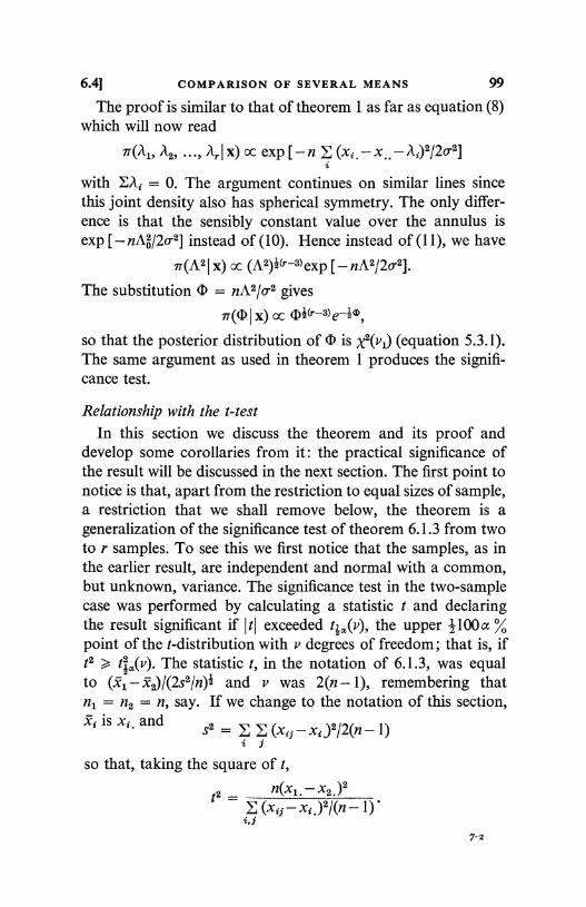
6.41 COMPARISON OF SEVERAL MEANS 99
The proof is similar to that of theorem 1 as far as equation (8)which will now read
7T(11, )(2, ..., xr I x) oc exp [ - n (xi. - x - )(i)2/2o-11
with EAi = 0. The argument continues on similar lines sincethis joint density also has spherical symmetry. The only differ-ence is that the sensibly constant value over the annulus isexp [-nA2/2o-2] instead of (10). Hence instead of (11), we have
-7r(A2I x) cC (A2)l(r-3)exp [ - nA2/2o 2].
The substitution I = nA2/o'2 gives
?r((D I x) cc (jj (r-3)e-t,0,
so that the posterior distribution of t is x2(v1) (equation 5.3.1).The same argument as used in theorem 1 produces the signifi-cance test.
Relationship with the t-testIn this section we discuss the theorem and its proof and
develop some corollaries from it: the practical significance ofthe result will be discussed in the next section. The first point tonotice is that, apart from the restriction to equal sizes of sample,a restriction that we shall remove below, the theorem is ageneralization of the significance test of theorem 6.1.3 from twoto r samples. To see this we first notice that the samples, as inthe earlier result, are independent and normal with a common,but unknown, variance. The significance test in the two-samplecase was performed by calculating a statistic t and declaringthe result significant if Itl exceeded t1a(v), the upper 1100a %point of the t-distribution with v degrees of freedom; that is, ift2 tia(v). The statistic t, in the notation of 6.1.3, was equalto (x1- x2)/(2s2/n)i and v was 2(n - 1), remembering thatn1 = n2 = n, say. If we change to the notation of this section,xi is xi, and s2 = E E (xij - x1)2/2(n - 1)
so that, taking the square of t,
t2 =n(xi. - x2. )2
((xiJ - xi.)2/(ni, 3
7-2
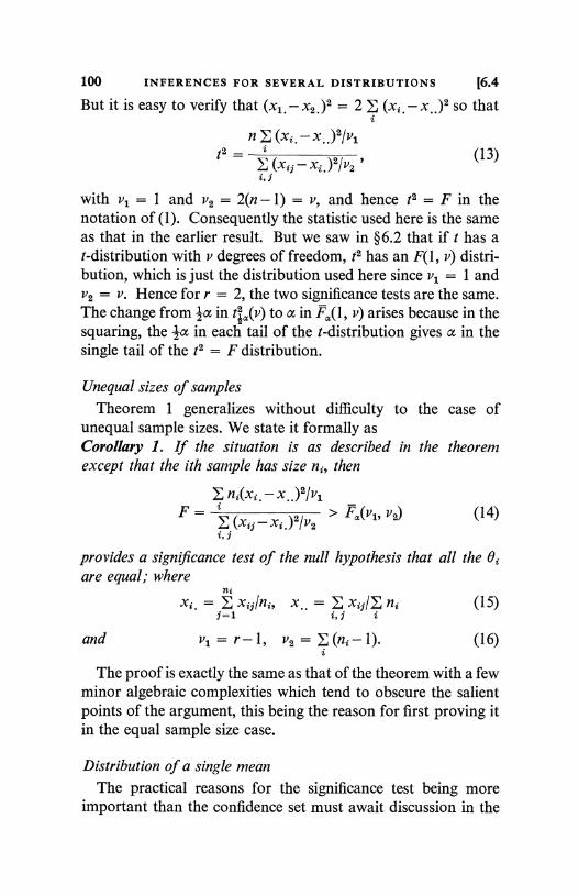
100 INFERENCES FOR SEVERAL DISTRIBUTIONS [6.4
But it is easy to verify that (x1, - x2,)2 = 2 E (xi. - so that
n (xi - x..)2/v122 =t
(xij - x1.)2/v2
i
(13)
with v1 = 1 and v2 = 2(n - 1) = v, and hence t2 = F in thenotation of (1). Consequently the statistic used here is the sameas that in the earlier result. But we saw in § 6.2 that if t has at-distribution with v degrees of freedom, t2 has an F(1, v) distri-bution, which is just the distribution used here since v1 = 1 andv2 = v. Hence for r = 2, the two significance tests are the same.The change from Ia in t,a(v) to a in FP(l, v) arises because in thesquaring, the Ja in each tail of the t-distribution gives a in thesingle tail of the t2 = F distribution.
Unequal sizes of samplesTheorem 1 generalizes without difficulty to the case of
unequal sample sizes. We state it formally asCorollary 1. If the situation is as described in the theoremexcept that the ith sample has size ni, then
E ni(xi,-x..)2/v1 _F_
(xij - x1.)2/v2 > F. vl, v2) (14)
provides a significance test of the null hypothesis that all the eiare equal; where
nixi. = Y. xi;lni, x.. = E xij/Z ni (15)
and v1 = r-1, v2 = (ni-1). (16)
The proof is exactly the same as that of the theorem with a fewminor algebraic complexities which tend to obscure the salientpoints of the argument, this being the reason for first proving itin the equal sample size case.
Distribution of a single meanThe practical reasons for the significance test being more
important than the confidence set must await discussion in the
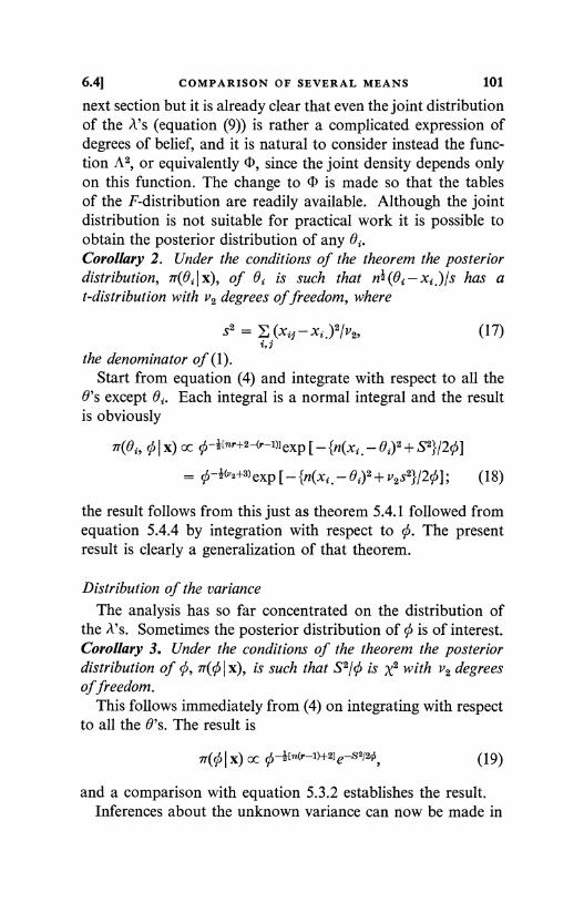
6.41 COMPARISON OF SEVERAL MEANS 101
next section but it is already clear that even the joint distributionof the A's (equation (9)) is rather a complicated expression ofdegrees of belief, and it is natural to consider instead the func-tion A2, or equivalently I, since the joint density depends onlyon this function. The change to is made so that the tablesof the F-distribution are readily available. Although the jointdistribution is not suitable for practical work it is possible toobtain the posterior distribution of any ei.Corollary 2. Under the conditions of the theorem the posteriordistribution, nr(eiJx), of ei is such that ni(ei-xi,)/s has at-distribution with v2 degrees of freedom, where
s2 = (xii -xi.)2Iv2, (17)
the denominator of (1).Start from equation (4) and integrate with respect to all the
O's except O. Each integral is a normal integral and the resultis obviously
7T(ei, 0 I x) a c-l [nr+2-(r-1)] exp [ - ln(xi. - 0,)2+S2 1/20]
= 0-l(va+3) exp [ - {n(xi. - ei)2 + V2 S2}/20]; (18)
the result follows from this just as theorem 5.4.1 followed fromequation 5.4.4 by integration with respect to 0. The presentresult is clearly a generalization of that theorem.
Distribution of the varianceThe analysis has so far concentrated on the distribution of
the A's. Sometimes the posterior distribution of 0 is of interest.Corollary 3. Under the conditions of the theorem the posteriordistribution of 0, 7r(o I x), is such that S2/¢ is x2 with v2 degreesof freedom.
This follows immediately from (4) on integrating with respectto all the 6's. The result is
7r(o I X) ccO-J[n(r-l)+2]e -S2/20, (19)
and a comparison with equation 5.3.2 establishes the result.Inferences about the unknown variance can now be made in
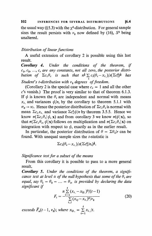
102 INFERENCES FOR SEVERAL DISTRIBUTIONS [6.4
the usual way (§ 5.3) with the x2-distribution. For general samplesizes the result persists with v2 now defined by (16), S2 beingunaltered.
Distribution of linear functionsA useful extension of corollary 2 is possible using this last
result.Corollary 4. Under the conditions of the theorem, ifc1i c2, ..., Cr are any constants, not all zero, the posterior distri-bution of Eci 0i is such that nI E ci(ei - x;.)/s(Ecz)i has
iStudent's t-distribution with v2 degrees of freedom.
(Corollary 2 is the special case where ci = 1 and all the otherc's vanish.) The proof is very similar to that of theorem 6.1.3.If ¢ is known the Oi are independent and normal with meansxi. and variances 0/n, by the corollary to theorem 5.1.1 witho --> oo. Hence the posterior distribution of Eci Oi is normal withmean Ecixi. and variance Ec?c/n by theorem 3.5.5. Hence weknow 9r(Eci 01 0, x) and from corollary 3 we know 7r(c I x), sothat 7r(EciBi, 0 x) follows on multiplication and HH(EciOiIx) onintegration with respect to 0, exactly as in the earlier result.
In particular, the posterior distribution of 0 = E0i/r can befound. With unequal sample sizes the t-statistic is
Eci(0i - xi.)1s(Eci1ni)i.
Significance test for a subset of the meansFrom this corollary it is possible to pass to a more general
result.Corollary 5. Under the conditions of the theorem, a signifi-cance test at level a of the null hypothesis that some of the 0i areequal, say 01 = 02 = ... = et, is provided by declaring the datasignificant if t
n Z (xi.-x(1).)2/(t- 1)F = z=1 (20)E (xi5-xi.)2/v2
i1jt
exceeds Fa(t-1, v2); where x(j). _ E xi./t.i-1

6.4] COMPARISON OF SEVERAL MEANS 103
The joint posterior distribution of 01, 02, ..., 0t and 0 isprovided by integrating (4) with respect to 0t+1, ..., 0r. Theresult is clearly
r(01, 02, ..., 0t, ¢ I x)
OClS-l[(nr+2)-(r-t)1eXp C - j n(x.. - 0;)2 + S21
/ 20, (21)
L ti-1U1and the result follows from (21) in the same way that thetheorem followed from (4). Notice that the numerator of (20)contains only those samples whose means are in question,whereas the denominator contains contributions from allsamples, as before. It is the same with the degrees of freedom:for the numerator they are reduced from (r-1) to (t-1) butthey stay the same, at r(n- 1), in the denominator.
It is worth noting that it follows from the form of the likeli-hood, which is proportional to the expression on the right-handside of (4) multiplied by 0, and the factorization theorem 5.5.2that (xl., x2., ..., xr., S2) are jointly sufficient for (01, 02iAll the posterior distributions quoted are in terms of thesestatistics.
Theorem 2 covers the situation where the variance is known.It is possible to see that the test statistic proposed, equation (12),is the natural analogue of (1), used when .2 is unknown, because,since o.2 does not have to be estimated, the denominator of (1)can be replaced by o.2 (see §6.5). This theorem has corollariesanalogous to those for theorem 1.
Derivation of the densityThere is one part of the proof that involves a type of argument
that has not been used before and is therefore worth some com-ment. This is the derivation of the density of A2. On manyoccasions we have had to integrate a joint density in order toobtain the density of a single random variable; but in these casesthe joint density has been expressed already in terms of the singlerandom variable required and others. But here we are requiredto obtain 1r(A2 I x) by integration of 7T(A1, A2, ..., k I x) where thelatter is not already expressed as a density of A2 and otherrandom variables. One method would be to rewrite
7T(A1, A2, , k I x)
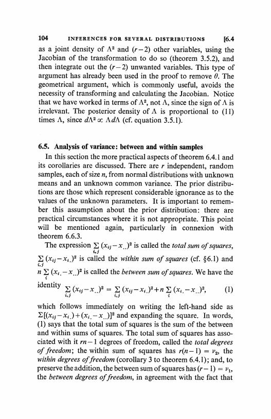
104 INFERENCES FOR SEVERAL DISTRIBUTIONS [6.4
as a joint density of A2 and (r-2) other variables, using theJacobian of the transformation to do so (theorem 3.5.2), andthen integrate out the (r-2) unwanted variables. This type ofargument has already been used in the proof to remove 0. Thegeometrical argument, which is commonly useful, avoids thenecessity of transforming and calculating the Jacobian. Noticethat we have worked in terms of A2, not A, since the sign of A isirrelevant. The posterior density of A is proportional to (11)times A, since dA2 cc AdA (cf. equation 3.5.1).
6.5. Analysis of variance: between and within samplesIn this section the more practical aspects of theorem 6.4.1 and
its corollaries are discussed. There are r independent, randomsamples, each of size n, from normal distributions with unknownmeans and an unknown common variance. The prior distribu-tions are those which represent considerable ignorance as to thevalues of the unknown parameters. It is important to remem-ber this assumption about the prior distribution: there arepractical circumstances where it is not appropriate. This pointwill be mentioned again, particularly in connexion withtheorem 6.6.3.
The expression Z (xij - is called the total sum of squares,i, I
(xi;-xi.)2 is called the within sum of squares (cf. §6.1) and10n E (xi, - is called the between sum of squares. We have the
iidentity
(xj-x..)2 = E (xj-xi.)2+n (xi.-x..)2, (1)i,j
which follows immediately on writing the left-hand side asE [(xij - xi _) + (xi. - x..)]2 and expanding the square. In words,(1) says that the total sum of squares is the sum of the betweenand within sums of squares. The total sum of squares has asso-ciated with it rn -1 degrees of freedom, called the total degreesof freedom; the within sum of squares has r(n -1) = v2, thewithin degrees of freedom (corollary 3 to theorem 6.4.1); and, topreserve the addition, the between sum of squares has (r - 1) = vl,the between degrees of freedom, in agreement with the fact that
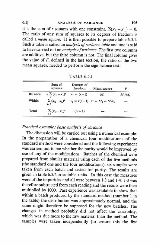
6.5] ANALYSIS OF VARIANCE 105
it is the sum of r squares with one constraint, E(xi,-x,.) = 0.The ratio of any sum of squares to its degrees of freedom iscalled a mean square. It is then possible to prepare table 6.5.1.Such a table is called an analysis of variance table and one is saidto have carried out an analysis of variance. The first two columnsare additive, but the third column is not. The final column givesthe value of F, defined in the last section, the ratio of the twomean squares, needed to perform the significance test.
TABLE 6.5.1
Sum of Degrees ofsquares freedom Mean square F
Between n E vl = (r-1) M1 M11M2i
Within E (xz1-xi,)2 v, = r(n-1) ss = M, = Sa/ve -i,a
Total (nr-1)
Practical example: basic analysis of varianceThe discussion will be carried out using a numerical example.
In the preparation of a chemical, four modifications of thestandard method were considered and the following experimentwas carried out to see whether the purity would be improved byuse of any of the modifications. Batches of the chemical wereprepared from similar material using each of the five methods(the standard one and the four modifications), six samples weretaken from each batch and tested for purity. The results aregiven in table 6.5.2 in suitable units. In this case the measureswere of the impurities and all were between 1.3 and 1.4: 1.3 wastherefore subtracted from each reading and the results were thenmultiplied by 1000. Past experience was available to show thatwithin a batch produced by the standard method (number 1 inthe table) the distribution was approximately normal, and thesame might therefore be supposed for the new batches. Thechanges in method probably did not affect the variability,which was due more to the raw material than the method. Thesamples were taken independently (to ensure this the five
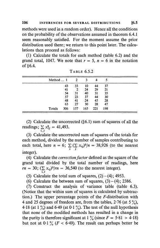
106 INFERENCES FOR SEVERAL DISTRIBUTIONS [6.5
methods were used in a random order). Hence all the conditionson the probability of the observations assumed in theorem 6.4.1seem reasonably satisfied. For the moment assume the priordistribution used there; we return to this point later. The calcu-lations then proceed as follows:
(1) Calculate the totals for each method (table 6.2) and thegrand total, 1047. We note that r = 5, n = 6 in the notationof § 6.4.
TABLE 6.5.2
Method ... 1 2 3 4 5
43 33 10 44 37
41 2 24 29 21
54 31 40 31 35
57 23 37 44 30
48 41 24 45 28
63 27 30 28 47
Totals 306 157 165 221 198
(2) Calculate the uncorrected (§6.1) sum of squares of all thereadings; E x45 = 41,493.
i1i(3) Calculate the uncorrected sum of squares of the totals for
each method, divided by the number of samples contributing toeach total, here n = 6; (E x25)2/n = 38,926 (to the nearest
i jinteger).
(4) Calculate the correction factor defined as the square of thegrand total divided by the total number of readings, herern = 30; (E x;f)2/rn = 36,540 (to the nearest integer).
i,t(5) Calculate the total sum of squares, (2) - (4) ; 4953.(6) Calculate the between sum of squares, (3) - (4); 2386.(7) Construct the analysis of variance table (table 6.3).
(Notice that the within sum of squares is calculated by subtrac-tion.) The upper percentage points of the F-distribution with4 and 25 degrees of freedom are, from the tables, 2.76 (at 5 %),4.18 (at 1 %) and 6.49 (at 0.1 %). The test of the null hypothesisthat none of the modified methods has resulted in a change inthe purity is therefore significant at 1 % (since F = 5.81 > 4.18)but not at 0.1 % (F < 6.49). The result can perhaps better be
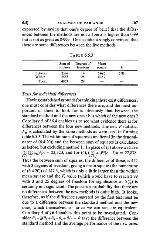
6.5] ANALYSIS OF VARIANCE 107
expressed by saying that one's degree of belief that the differ-ences between the methods are not all zero is higher than 0.99but is not as great as 0.999. One is quite strongly convinced thatthere are some differences between the five methods.
TABLE 6.5.3
Sum ofsquares
Degrees offreedom
Meansquare F
Between 2386 4 596.5 5.81Within 2567 25 102.7 -
Total 4953 29 - -Tests for individual differences
Having established grounds for thinking there exist differences,one must consider what differences there are, and the most im-portant of these to look for is obviously that between thestandard method and the new ones: but which of the new ones?Corollary 5 of §6.4 enables us to see what evidence there is fordifferences between the four new methods. The new F statistic,F4i is calculated by the same methods as were used in formingtable 6.5.3. The within sum of squares is unaltered (in the denomi-nator of (6.4.20)) and the between sum of squares is calculatedas before, but excluding method 1. In place of (3) above we haveZ (y x;)2/n = 23,320, and for (4), x2;)2/(r-1)n = 22,878.
i>l,fThus the between sum of squares, the difference of these, is 442with 3 degrees of freedom, giving a mean square (the numeratorof (6.4.20)) of 147.3, which is only a little larger than the withinmean square and the F4 value (which would have to reach 2.99with 3 and 25 degrees of freedom for significance at 5 %) iscertainly not significant. The posterior probability that there areno differences between the new methods is quite high. It looks,therefore, as if the difference suggested by the first test must bedue to a difference between the standard method and the newones, which themselves, so far as we can see, are equivalent.Corollary 4 of § 6.4 enables this point to be investigated. Con-sider BI - *(B2 + 03 + 04 + 05) = 0 say: the difference between thestandard method and the average performance of the new ones.
108 INFERENCES FOR SEVERAL DISTRIBUTIONS [6.5
Since Ec = 1.25, x1 20.125, V2 = 25and s2 = 102.7 (within degrees of freedom and mean square),the confidence limits for 0 are
20.125 ± t1a(25) x (102-7x 1.25/6)1
with confidence coefficient 1- a. At 5 % the t-value is 2.06 andthe limits are (10.6, 29.7). At 0.1 % with a t-value of 3.72 thelimits are (2.9, 37.3), which exclude the origin, so that thedifference is significant at 0.1 %.
The results of the experiment may be summarized as follows:(i) There is no evidence of any differences between the four
new methods.(ii) The average effect of the new methods is to reduce the
impurity as compared with the standard method. The effect isestimated to lie most likely (with 95 % confidence) between areduction of 0.0106 and 0.0297, and almost certainly (99.9 %confidence) to lie between 0.0029 and 0.0373: the most probablevalue is 0.0201.
A better way to express this would be to say that this reduc-tion 0 was such that
f0--0-0201}/0-00463
had a posterior distribution which was Student's t on 25 degreesof freedom.
Form of the F-statisticThe computational method is merely a convenient way of
arranging the arithmetic in order to obtain the required F-ratio.But since the sufficient statistics (the xi and S2) are found indoing this, it is suitable for any inference that one wishes tomake. Let us first look at this F-statistic. In the language of thedefinitions given above it is the ratio of the between mean squareto the within mean square. An extension of the discussion in§6.1 shows that the within mean square, being the ratio of thesum of sums of squares for each sample, ES?, and the sumof the separate sample degrees of freedom, is a natural estimateto replace the unknown 0; and this, whatever be the values ofthe 6j. A similar discussion shows that if the null hypothesis istrue, so that the xi _ are independent and normal with the samemean and variance qi/n, then E(xi, - divided by its degrees
6.5] ANALYSIS OF VARIANCE 109
of freedom, (r - 1), is an estimate of 0/n. Hence when the nullhypothesis is true the between mean square, nE(x2. - x..)2/(r -1),is also an estimate of 0, and F is the ratio of two such estimates,and is therefore about 1. When the null hypothesis is not truethe between mean square will be larger since the x2. will be morescattered because the B2 are. Consequently F will be typicallygreater than 1. This shows that the test, which says that the nullhypothesis is probably not true when F is large, is sensible onintuitive grounds.
Notice that the sums of squares are all calculated by sub-tracting a squared sum from an uncorrected sum of squares(cf. § 5.4). Thus the between sum of squares is
nE(x2.-x..)2 = nEx4 .-nrx2.
(F+ x;)2/n - (Z X j)2/rn, (2)
and the total sum of squares is
E'(x2;-x..)2 = Exit-(ExA)2/rn. (3)
It is useful to notice that whenever a quantity in the form ofa sum is squared, it is always, after squaring, divided by thenumber of x2f that were added up to give the quantity. Thus, in(2), (Z x21)2 is divided by n because x2f is the sum of n terms.
The within sum of squares could be found by calculating eachS2 and adding, but it is computationally easier to use (1).
The calculations proceed in essentially the same manner whenthe sample sizes are unequal. In (2) we have to calculate
{(Z x2 f)2/n2}, in agreement with the sentence after equation (3) :i I
but otherwise there is no change in the method. Notice, too,that the calculations are much simplified by changing origin andscale to reduce the magnitudes and avoid the troubles ofnegative values. A desk calculating machine is essential forall but the smallest analyses.
Extended analysis of variance tableThe additivity of the sums of squares can be extended still
further. We saw in the last section that the F-test was a generali-zation of the t-test, and a t-test could be put in an F form by
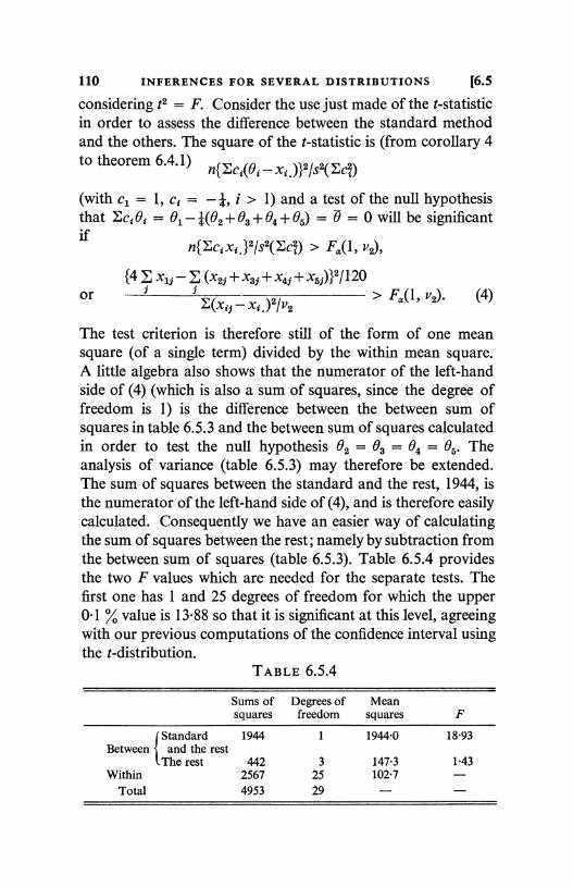
110 INFERENCES FOR SEVERAL DISTRIBUTIONS [6.5
considering t2 = F. Consider the use just made of the t-statisticin order to assess the difference between the standard methodand the others. The square of the t-statistic is (from corollary 4to theorem 6.4.1)
n{Eci(0i-xi.)}2Is2(Ec4,,)
(with c1 = 1, ci = -1, i > 1) and a test of the null hypothesisthat Eci Oi = 01- 4(02 + 03 + 04 + 05) = B = 0 will be significantif
or
n{Ecixi.}2/S2(Eci) > F, (I, v2),
{4 x1j - (x27 + X3.7 + x47 + x51)}2/ 1207 7 F 1 4
E(xi1 - xi. )2/v2> a( , V2) ( )
The test criterion is therefore still of the form of one meansquare (of a single term) divided by the within mean square.A little algebra also shows that the numerator of the left-handside of (4) (which is also a sum of squares, since the degree offreedom is 1) is the difference between the between sum ofsquares in table 6.5.3 and the between sum of squares calculatedin order to test the null hypothesis 02 = 03 = 04 = 05. Theanalysis of variance (table 6.5.3) may therefore be extended.The sum of squares between the standard and the rest, 1944, isthe numerator of the left-hand side of (4), and is therefore easilycalculated. Consequently we have an easier way of calculatingthe sum of squares between the rest; namely by subtraction fromthe between sum of squares (table 6.5.3). Table 6.5.4 providesthe two F values which are needed for the separate tests. Thefirst one has 1 and 25 degrees of freedom for which the upper0.1 % value is 13.88 so that it is significant at this level, agreeingwith our previous computations of the confidence interval usingthe t-distribution.
TABLE 6.5.4
Sums ofsquares
Degrees offreedom
Meansquares F
Between and the restCheThe rest
1944
442
1
3
19440
147.3
1893
1.43Within 2567 25 102.7 -
Total 4953 29 - -
6.51 ANALYSIS OF VARIANCE 111
This breakdown of the total sum of squares into additiveparts is capable of important generalizations, some of whichwill be touched on in later sections (§§8.5, 8.6), but it is mainlyuseful as a computational device. The real problem is to expressconcisely the salient features of the joint posterior distributionof the A's (equation 6.4.9), and ideally this should lead at leastto confidence interval statements. These are usually obtained bydoing preparatory significance tests to see what differences, ifany, are important and estimating these. The numerical exampleis typical in this respect : only the difference between the standardmethod and the rest was significant and the posterior densityof that alone, instead of the joint density, needed to be quoted.
The variance estimation
It is sometimes useful to consider the variance 0. In virtue ofcorollary 3 to theorem 6.4.1 inferences about it can be madeusing the x2-distribution in the usual way (§ 5.3). The within sumof squares divided by ¢ is x2 with v2 degrees of freedom, so that
x2(25) < 2567-1 < x2(25).
At the 5 % level, the upper and lower points are respectively13.51 and 41.66, from the Appendix, so that the 95 % confidencelimits for 0 are (61.6, 190-0): the mean square being 102.7.The limits for the standard deviation, in the original units, aretherefore (0.0079, 0.0138). Notice that there are usually a largenumber of degrees of freedom available for error so that 0 isusually tolerably accurately determined.
If 0 is known, equal to 0.2, then theorem 6.4.2_is applicable.There is then no need to use the within sum of squares, whichonly serves to estimate 0, since it is already known. Instead theratio of the between sum of squares (not the between meansquare) to o.2 provides the necessary test statistic, which isreferred to the x2-table with (r - 1) degrees of freedom. One wayof looking at this is to say that when 0 is known, equal to 0.2, wehave effectively an infinity of degrees of freedom for the withinmean square and we saw (§6.2) that in these circumstancesv1F(v1, oo) was the same as a x2-distribution. The other devices
112 INFERENCES FOR SEVERAL DISTRIBUTIONS [6.5
used in this section extend to this case with the infinite degreesof freedom replacing v2.
If 0-2 is known it is possible to provide a check on the data byusing corollary 3 to theorem 6.4.1 to provide a test of the nullhypothesis that 0 = 0'2 in the usual way.
Prior distributions
In any application of the analysis of variance it is importantto remember the assumptions about the probability of the obser-vations: independence, normality, and constancy of variance.But it is also as well to remember the assumptions about theprior knowledge, particularly concerning the means. These aresupposed independent and uniformly distributed, where thelatter distribution is an approximation for a distribution of thetype discussed in § 5.2. Whilst any 0 may have this distributionit is not always reasonable to suppose them independent. Forexample, in the chemical illustration the impurity measure maywell fluctuate substantially depending on the raw material. Thisfluctuation was minimized here by making up the five batchesfrom similar material. Although one might be very vague aboutthe average value of the B's, or about any one of them, becauseof one's vagueness about the raw material, one might well feelthat any two of the 9's would be close together, precisely becausethe batches had been made from similar material. In the nextsection we shall show how some allowance can be made for thisin the case where 0 is known, equal to 0.2, say.
6.6. Combination of observationsOur topic is again that of several independent samples from
normal distributions, but we no longer consider differences ofmeans. In the first two theorems the means are supposed equaland the samples are combined to provide an inference about thecommon value. In the third theorem another sort of combina-tion is considered.
Theorem 1. Let Yi = (x21, x22, ..., xin) (i = 1, 2, ..., r) be r in-dependent random samples of sizes n1 from N(6, a% where the o-2are known but the common mean, 0, is unknown. Then if 0 has
6.6] COMBINATION OF OBSERVATIONS 113
a uniform prior distribution over (- co, co), the posterior distribu-tion of 0 is N(x,,, (Ewi)-1) where
x = Ewixi./Ewi and w.,-1 = ozlni (1)
wi is called the weight of the ith sample, and x., the weighted mean(§ 5.1).
The likelihood of 0 from the ith sample is given, apart fromthe unnecessary constant of proportionality, by equation 5.1.9;and hence the likelihood from all r samples is the product ofthese. Thus, if x denotes the set of all xi;, and xi. _ Exi;lni,
jp(x B) oc exp [ - I Ewi(xi, - 0)2]
oc exp [-4Ewi02+ Ewixi,B]
oc exp [-i(Ewi) (0- Ewixi./Ewi)2] (2)
Since IT(O) is constant, 7r(B I x) is also proportional to (2), whichproves the theorem. (An alternative proof is given below.)
Theorem 2. Let the conditions be as in theorem 1 except that0-4 = 04, where the T's are known but 0 is not. Then if ln¢ hasa uniform prior distribution over (- oc, oo) independent of 0, theposterior distribution of 0 is such that
(Ewi)' (0-9-W (3)
has Student's t-distribution with v = (Eni - 1) degrees offreedom,where
andX = EWixi./Ewi, wi 1 = T2/ni (4)
S2 = [ (xj - xi.)2/r4 + F+ wi(xi. - x..)2]/v = [ (x3 - g..)2/7-fl/V.i,f
(5)
The likelihood now involves 0 which cannot be absorbed intothe constant of proportionality as in the proof of theorem 1.From the normal density for each xif the likelihood is easilyseen to be
p(x I e, 0) cc 0-4cv+l) exp [ - E (xf - 0)2/2T40], (6)
and hence 7r(O, 0 1 x) is proportional to the same expressionmultiplied by 0-1. To simplify this, collect together like termsin the exponential in 0 and 02 in order to have a single term
8 LSII
114 INFERENCES FOR SEVERAL DISTRIBUTIONS [6.6
involving 0 (compare the argument leading to equation 5.4.4).The expression in square brackets is - l/2q times
02 nil r4 - 26 xij/T i + E xi/Ti
/O2(E 0i)-28 xi.Wi+ E (x;-xi.)2/r1+ E nix Q /T1
=(Z 17V) (0-2 )2+£(xi;-xi.)2/r4 +Ewix2.-(Ewi)XE
The terms not involving 02 clearly reduce to vs"2. Hence
ir(e, c I x) cco-llv+s> exp [ - {(E N'i) (0 - x.. )2 + vs 2}/2c] (7)iThe result follows from (7) in the same way that theorem 5.4.1followed from equation 5.4.4. The alternative expression for s2in (5) follows easily (cf. equation 6.5.1).
In the following theorem we use vector and matrix notation.x denotes a column vector, and x' its transpose, a row vector,with elements (x1, x2, ..., xn). Capital letters denote squarematrices (cf. §§3.3, 3.5).
Theorem 3. If the random variables x have a multivariate normaldistribution with expectations e(x) = AO, where A is known but0 = (01, 02, ..., 0p) is not, and known dispersion matrix C; and ifthe prior distribution of 0 is multivariate normal with expectationsd'(9) = tLo and dispersion matrix CO; then the posterior distribu-tion of 0 is also multivariate normal with expectations
NL1 = {Co I+ A'C-'A}-1 {Co1t0 + A'C-lx} (8)
and dispersion matrix{Co 1 + A'C-'A}-1. (9)
From the expression for the normal multivariate density(equation 3.5.17), written in the vector notation, we have, sincethe dispersion matrix is known,
p(x I 9) oc exp { - M(x - A9)' C-1(x - A8)} (10)
and IT(9) cc exp{ -+(9 - to)' Co 1(e - µo)}. (11)
Hence n-(O I x) is proportional to the product of these two expo-nential(. The resulting single exponential we manipulate in the
6.61 COMBINATION OF OBSERVATIONS 115
same way as in the last theorem, discarding into the omittedconstant any multiplicative terms not involving 0. Thus,
ir(O I x) cc exp { - z [®'(Co 1 + A'C-'A) 0 - 20'(Co 1p. o + A'C-1x)]}
oc exp { - z [(0 - I.1)' (Co 1 + A'C-1A) (0 - FL1)]}.
A comparison of this last result with the normal density, (11),establishes the result.
Combinations of inferencesIn calling this section `combination of observations' we are
extending the original meaning of this phrase, which referred tothe results of the type discussed in §3.3, and made no referenceto degrees of belief. Our excuse for the extension is that theearlier results were (and indeed are) used in an inference sensewhich is justified by the above results. In amplification of thispoint consider a simple typical result obtained in §3.3. If x1 andx2 are two independent, unbiased determinations of an unknownIt, then 2 (x1 + x2) is another unbiased determination. Further-more, 2 (x1 + x2) is typically a more precise determination thaneither x1 or x2 separately. Precisely, if
92(x,) = 0-2, C9i 2 [+(x1 +x2) ] = 1(0.1 +0.1
However, there are two things that remain to be discussed.What inferences can be made about ,u given xl and x2; and is4(x1 + x2) the best determination? If the additional assumptionof normality of x1 and x2 is made we shall see how to answerboth these questions. The inference part is simple since we havealready seen how a statement about a normal random variablecan easily be turned into a statement of belief about its mean.(Compare the statements (a) and (b) in §5.1.) Thus, in theexample, It, given Mx1 + x2), is normally distributed about+2(x1 + x2) with variance *(0-i + 0-2) provided the prior knowledgeof ,u is vague. In answer to the second question we now showthat the ordinary average, J(x1 + x2), is not necessarily the bestdetermination of it.
Theorem 1 provides an answer to the question: if severalindependent determinations are made of the same unknownwith different precisions, then how should they be combinedinto a single determination, and what precision has this?
8-2
116 INFERENCES FOR SEVERAL DISTRIBUTIONS [6.6
First consider any sample. In the language of §3.3 this formsa set of n, determinations of an unknown (now denoted by 0)with equal precisions o-i 2. (In §5.1 the precision was defined asthe inverse of the variance.) The results of §5.1 show that,because of the normality, the mean is sufficient and forms adetermination of precision n2/o4, the w2 of the theorem. So muchis familiar to us. The new point is to discover how the separatedeterminations from the different samples should be combined.The answer is to use the weighted mean (§5.1) with the inversesof the variances as weights: that is, the precisions of eachdetermination. This is intuitively sensible since the larger thevariance the smaller the precision or weight.
Relationship with Bayes's theoremThe result is very similar to the corollary to theorem 5.1.1,
where a weighted mean was used to combine prior knowledgewith the determination. In fact, the present theorem can bededuced from the corollary in the following way. Consider thesamples taken one at a time, and apply the corollary each timea new sample is taken. Initially, in the notation of the corollary,we let vo -,_ oo; the posterior distribution after the first samplebeing N(xl., o /n1). Now proceed to the second sample. Theprior distribution now appropriate; that is, the distributionexpressing one's present beliefs about 0, is the posterior distribu-tion derived from the first sample, N(xl., o f/n1). Use of thecorollary with Ito = xl., 002 = o /n1 gives a posterior distributionafter the second sample which is
N[(w1 x1 + w2 x2)/(wl + w2), (w1 + w2)-1l,
the precisions of the first sample (now the prior precision) andthe second sample being added, and the means weighted withthem. Continuing in this way to r samples we have the generalresult. This second proof is interesting because it shows howone's beliefs change in a sequence as the new samples becomeavailable, and how the posterior distribution after one set ofobservations, or samples, becomes the prior distribution for thenext set of observations.
6.61 COMBINATION OF OBSERVATIONS 117
Case of unknown variancesNotice that in order to make the best determination, namely
the weighted mean, it is only necessary to know the ratios of theweights, or the precisions, or the variances ul. (Their absolutevalues are needed for the precision of the best determination.)Theorem 2 is available when these ratios are known but thefinal precision has to be estimated because the absolute valuesare not known. It is often useful when of is known to beconstant, but there are other situations of frequent occurrencewhere the relative precisions are known but the absolute valuesare not. An example is where two instruments have been used,one of which is known to have twice the precision of the otherwhen used on the same material, but where the actualprecision depends on the material.
The result is best appreciated by noting that it is an exten-sion of theorem 1 in the same way that Student's result(theorem 5.4.1) is an extension of theorem 5.2.1: namely thevariance is estimated by a mean square, and the t-distributionreplaces the normal. Thus if the result of theorem 1 is written,(Ewi)I (0 - is N(0, 1), or, in the notation of theorem 2,(Ewi)I is N(0, 1), the comparison is obvious exceptfor the apparently rather unusual estimate, s, that replaces 01.The form of s can be easily understood by using analysis ofvariance terminology of the last section. We have seen in §6.1that several estimates of variance should be combined by addingthe sums of squares and adding the degrees of freedom, anddividing the former by the latter. In the situation of theorem 2each sample provides an estimate of variance, the sum ofsquares for the ith sample being (x; - xi.)2. But this sample
has variance OT?, so (x,; - X,.)2/T4 is clearly the sum of squares
appropriate to . Summing these over the samples gives thewithin sum of squares, the first term in the first form for s2 in (5).But some more information is available about 0. The samplemeans x, have variances OT2/ni = 0w2 1, and hence xi.w, hasvariance 0. Taking the sum of squares of the xi. about theweighted mean z.. with weights wi gives Ewi(xi the
118 INFERENCES FOR SEVERAL DISTRIBUTIONS 16.6
remaining term in the first form for s2 in (5). This latter expres-sion is a generalization of the idea of the between sum of squaresto the case where the means have different variances of knownratios. The two expressions may be added to give the secondform for g2 in (5), and the part in square brackets is therefore thetotal sum of squares. The degrees of freedom are (ni-1) foreach sample; giving E(ni -1) = Eni - r, for the within sum, and(r - 1) for the between sum ; giving Eni - r + (r - 1) = Eni - 1 = v,in all. This last result is also intuitively reasonable since theEni readings have lost one degree of freedom for the singleunknown 0.
It would be useful to have an extension of theorem 1 to thecase where the of are unknown, but no simple result is available.The situation is complex because r integrations are needed (toremove each of the o ), and the distribution depends on manyparameters. The reader can compare the difficulties with thoseencountered in Behrens's problem (§6.3). There are two thingsone can do : if the o-4 are not likely to be too unequal then onecan assume them all equal to an unknown 0-2, and use theorem 2;alternatively, one can estimate oj in the usual way by
s? = E (xij - xi.)2/(ni -1),
replace a 2i by s4 and ignore any distributional changes thatmight result. The latter is only likely to be satisfactory if all thesample sizes are large so that the error in replacing of by si issmall.
Multivariate problemsThe alternative proof of theorem 1, using the corollary to
theorem 5.1.1, demonstrates a connexion between the combina-tion of observations and the combination of prior informationand likelihood, and therefore between theorem 1 and theorem 3,which is an extension of theorem 5.1.1 from one variable toseveral. (In the univariate case we can take A to be the unitmatrix.) It says that a multivariate normal prior distributioncombines with a multivariate normal likelihood to give a multi-variate normal posterior distribution. If A = I, the unit matrix
6.61 COMBINATION OF OBSERVATIONS 119
(necessarily p = n), then the inverses of the dispersion matricesadd (equation (9)) and the posterior mean is an average of thetwo means with weights equal to these inverses.
Example 1. We consider two applications of theorem 3. Thefirst is to the weighing example of § 3.3. In the discussion of thatexample in §3.3 we were concerned only with the variances ofcertain quantities (equations 3.3.2), suggested as determinationsof the weights. t We now use theorem 3 to show that thesedeterminations are the best possible. It is clear that the x, of§3.3 have expectations (equation 3.3.1)
'e(xl) = 01+02-63-04, (12)
etc., and that, granted the normality, they satisfy the conditionsof the theorem with
1 1 -1 -1
A -1 -1 -1 1
(13)
1 1 1 1
and C equal to the unit matrix times o.2. If the prior knowledgeof the true weights, 6i, is vague compared with 0-2, then CO-' maybe ignored and the posterior distribution of the true weights hasmean (equation (8)) equal to (A'A)-1A'x. An easy calculationshows that A'A is four times the unit matrix so that the mean isIA'x, the values given in equation 3.3.2. The dispersion matrixof the posterior distribution is (A'A)-1cr2: so that the variancesare all *o-2 and the covariances zero. Note that, apart from afactor 4, A is an orthogonal matrix (A'A = 41), hence the name,orthogonal experiment, used in § 3.2.
Example 2. The second example applies to the analysis ofvariance between and within samples discussed in §§ 6.4, 6.5.Suppose the situation to be that described in the statementof theorem 6.4.2 with 0 known, equal to 0-2, say. With-out loss of generality we can suppose n = 1 and denote theobservations by xti, since, with n > 1, {x2.} is sufficient. Thenthe likelihood is as in theorem 3 with A equal to the unit matrixof size r x r and C equal to the unit matrix times 0-2. In § 6.5 we
t The reader should be careful to avoid confusing the weights put on thebalance and the statistical weights of the observations.
120 INFERENCES FOR SEVERAL DISTRIBUTIONS [6.6
made the point that in the prior distribution the B= were notalways independent. Suppose that 0 is N(p.0, Co) with all theelements of V.0 equal to ,uo, say, and with Co having the specialform of a matrix with 0-0 2 down the leading diagonal and po-oeverywhere else: denote such a matrix by 1101, p0111. Then theBi have the same prior means ,uo and variances 002, and thecorrelation between any pair is p. In particular, for anyunequal i, j,
-92(Bi-O) = 2v0l(1-p), (14)
by theorem 3.3.2. This prior distribution is one in which the 02'sare all alike in means and variances, and are equally correlated.Some algebra is necessary to obtain the mean of the posteriordistribution, but this is considerably lightened by using the fact(which is easily verified) that if the matrices are of size r x r
Ila, bIj-1 = 11 [a+(r-2)b]c,-bcll
with c-11 = [a+(r-1)b] (a - b). (15)
It immediately follows from this result that
Co-' = 11[1+(r-2)p]A,-pAll
with A-1 = [l +(r- l)p] (I -p)°'o.
Now we are interested (as explained in §6.5) in cases where anyone 0, is vaguely known but any two are thought to be closetogether. We therefore consider the case where 0-u - oo but0-0 2(1-p) -* T2, say, which is finite: this will mean that p --j 1.From (14) it follows that the difference between any two 0 's hasfinite variance, 27.2, but the variance of any 0, tends to infinity.In this limit 11
Co 1 -
and Co 1 + C-1 =
Using (15) again, we obtain
r-1 1
rT2 ' rT2
r-l 1 _ 1
rT2 + Q2 rT
1 1 1
(rT2 Q2 rT2with 6-1 =
.2 + T2
Q4.T2 .
6.6] COMBINATION OF OBSERVATIONS 121
Since Co 1[L0 = 0 and C-1x has typical element xi/Q2, we havefor a typical element of [,1, the value
(Ti+aiXi+iT2j xjJ
l((Tcr2T22) 1/0-.2+1//22'
(16)
In words, the expected posterior value of Oi is a weighted meanof xi and the mean of the x's, x., with weights equal to the pre-cision of each xi and twice the precision of the prior differenceof any two Oi's. The effect is to replace the natural value, xi, forthe expectation of 0, by a value shifted toward the commonmean. The values of Oi with xi near x will be little affected, butthose with the extreme values of xi will be shifted to a greaterdegree towards x.. This is in satisfactory agreement withcommon-sense ideas for it is usual to feel that the extremevalues should be a little discounted just because they are extremevalues. For example, in the numerical illustration of §6.5 thesecond method had the lowest mean and was, on the evidenceof the experiment, the best; but one might not feel happy atsaying its expected value was 157/6 = 26.2 because it may justhave done rather well in this experiment: in another experimentmethod 3 might be lower.
General inference problemsTheorem 3 does not easily extend to deal with the case of
unknown o.2 and T2 in example 2 (evidence on these is availablefrom the within and between sums of squares respectively). Butit does show how prior knowledge should be incorporated intothe data. This is perhaps a convenient point to make the generalremark that every inference situation should be judged on itsown. In this book we give recipes that fit a wide class ofproblems but it should not be thought that these are the onlycases that arise. The best approach to any inference problem isto consider the likelihood and the prior distributions separatelyand then to form their product to obtain the posterior distribu-tion. If they fit into the framework of a standard method somuch the better, but if not, one can always try to put theposterior distribution into a convenient form and, if all elsefails, it can always be calculated numerically in any particular case.
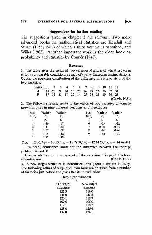
122 INFERENCES FOR SEVERAL DISTRIBUTIONS [6.6
Suggestions for further readingThe suggestions given in chapter 5 are relevant. Two moreadvanced books on mathematical statistics are Kendall andStuart (1958, 1961) of which a third volume is promised, andWilks (1962). Another important work is the older book onprobability and statistics by Cramer (1946).
Exercises1. The table gives the yields of two varieties A and B of wheat grown instrictly comparable conditions at each of twelve Canadian testing stations.Obtain the posterior distribution of the difference in average yield of thetwo varieties:
Station...1 2 3 4 5 6 7 8 9 10 11 12
A 25 28 28 20 23 23 26 29 26 26 37 31
B 17 15 21 18 22 14 25 28 25 19 34 25
(Camb. N.S.)2. The following results relate to the yields of two varieties of tomatogrown in pairs in nine different positions in a greenhouse:
Posi-tion,
i
VarietyX,x{
VarietyY,
Y,
Posi-tion,
i
VarietyX,x{
VarietyY,yi
1 1.39 1.17 6 1.63 1222 1.41 1.22 7 0.88 0.843 1.07 1.08 8 1.14 0.944 1.65 1.42 9 1.32 1255 1.57 1.39
(Ex{ = 12.06, Ey{ = 10.53, Ex; = 16.7258, Ey, = 12.6123, Exdy, = 14.4768.)Give 99 % confidence limits for the difference between the average
yields of X and Y.Discuss whether the arrangement of the experiment in pairs has been
advantageous. (Camb. N.S.)3. A new wages structure is introduced throughout a certain industry.The following values of output per man-hour are obtained from a numberof factories just before and just after its introduction:
Output per man-hour
Old wagesstructure
New wagesstructure
122.3 119.0141.0 131.81201 118.7109.6 106.0119.1 1182128.0 126.6132.8 124.1
EXERCISES 123
If 6 is the average change in output per man-hour over all factories in theindustry, consequent upon the change in wages structure, calculate, onconventional assumptions, 95 % confidence limits for 6 in each of thefollowing cases:
Case I. The data refer to seven different factories, corresponding figuresin the two series coming from the same factory.
Case II. The data refer to fourteen different factories.Suppose in case II that further values were obtained, making up n fac-
tories in each column instead of 7. Roughly how large would n have to befor one to be reasonably sure of detecting that 6 was not zero, if in fact9 was equal to - 2.0 units? (Manch. Dip.)4. Two normal populations of known equal variance do have means01i 02. It is required to calculate, from random samples of size n takenfrom each population, a 1002 % confidence interval for 0 = 02 - 01. Thefollowing procedure is suggested: 100x % confidence intervals are calcu-lated separately for 01 and 02 and are, say, (11, u1) and (12i u2). Any valuein (11, u1) is, at this probability level, a possible value for B1, and similarlyfor 02. Hence any value in the interval (12 - u1i u2 -11) is a possible valuefor 0 at confidence level 1002 % and is the confidence interval required.Explain why this argument is false and compare the answer it gives withthat obtained from the correct procedure. (Lond. B.Sc.)
5. It is expected that a certain procedure for estimating the percentageamount of a substance X in a sample of material will give a standard errorapproximately equal to 0.12. Two chemists take samples from a given bulkof material and each performs five independent determinations of thepercentage amount of X present in the material. Their readings are asfollows:
First chemist: 2.43, 2.42, 222, 2.29, 2.06Second chemist: 2.48, 2.72, 2.43, 2.40, 2.58
Do these figures support the assumption that the standard error of adetermination is 0.12? Is there any evidence that one chemist's readingsare biased relative to the other? (Camb. N.S.)
6. Two workers carried out an experiment to compare the repeatabilitieswith which they used a certain chemical technique. The first worker madeeight determinations on the test substance and estimated the standarddeviation of a single measurement as 0.74; the second worker made fifteendeterminations on the same substance and obtained a standard deviationof 1.28. Compare the repeatabilities of the two workers' measurements.
(Camb. N.S.)7. Two analysts each made six micro-analytical determinations of thecarbon content of a chemical, giving the values:
Analyst I: 59.09, 5917, 59.27, 59.13, 59.10, 59.14Analyst II: 59.06, 59.40, 59.00, 5912, 59.01, 59.25
Discuss whether these results provide evidence that the two analystsdiffer in their accuracy of determination. (Camb. N.S.)
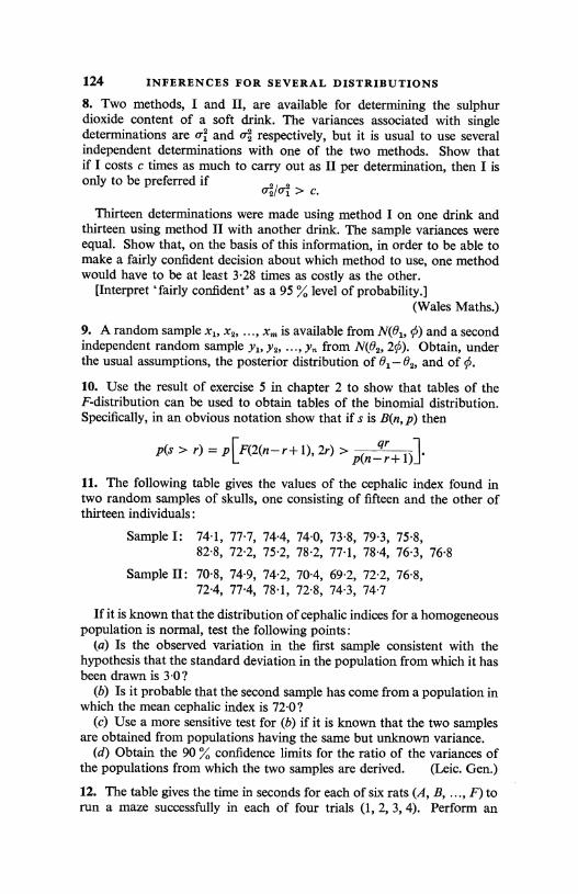
124 INFERENCES FOR SEVERAL DISTRIBUTIONS
8. Two methods, I and II, are available for determining the sulphurdioxide content of a soft drink. The variances associated with singledeterminations are and of respectively, but it is usual to use severalindependent determinations with one of the two methods. Show thatif I costs c times as much to carry out as II per determination, then I isonly to be preferred if 02/-2 > c
Thirteen determinations were made using method I on one drink andthirteen using method II with another drink. The sample variances wereequal. Show that, on the basis of this information, in order to be able tomake a fairly confident decision about which method to use, one methodwould have to be at least 3.28 times as costly as the other.
[Interpret `fairly confident' as a 95 % level of probability.](Wales Maths.)
9. A random sample x1i x2, ..., x,,, is available from N(01, 0) and a secondindependent random sample y1i y2, ..., y from N(02, 20). Obtain, underthe usual assumptions, the posterior distribution of 01-02i and of 0.
10. Use the result of exercise 5 in chapter 2 to show that tables of theF-distribution can be used to obtain tables of the binomial distribution.Specifically, in an obvious notation show that ifs is B(n, p) then
AS > r) = P [F(2(n-r+ 1), 2r) > qrJ.p(n-r+ 1)
11. The following table gives the values of the cephalic index found intwo random samples of skulls, one consisting of fifteen and the other ofthirteen individuals:
Sample I: 74.1, 77.7, 74.4, 74.0, 73.8, 79.3, 75.8,82.8, 72.2, 75.2, 78.2, 77.1, 78.4, 76.3, 76.8
Sample II: 70.8, 74.9, 74.2, 70.4, 69.2, 72.2, 76.8,72.4, 77.4, 78.1, 72.8, 74.3, 74.7
If it is known that the distribution of cephalic indices for a homogeneouspopulation is normal, test the following points:
(a) Is the observed variation in the first sample consistent with thehypothesis that the standard deviation in the population from which it hasbeen drawn is 3.0?
(b) Is it probable that the second sample has come from a population inwhich the mean cephalic index is 72.0?
(c) Use a more sensitive test for (b) if it is known that the two samplesare obtained from populations having the same but unknown variance.
(d) Obtain the 90 Y. confidence limits for the ratio of the variances ofthe populations from which the two samples are derived. (Leic. Gen.)
12. The table gives the time in seconds for each of six rats (A, B, ..., F) torun a maze successfully in each of four trials (1, 2, 3, 4). Perform an
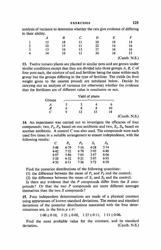
EXERCISES 125
analysis of variance to determine whether the rats give evidence of differingin their ability.
1
A15
B18
C11
D18
E19
F14
2 10 15 11 22 14 16
3 13 16 13 17 16 16
4 14 16 11 16 14 15
(Camb. N.S.)
13. Twelve tomato plants are planted in similar pots and are grown undersimilar conditions except that they are divided into three groups A, B, C offour pots each, the mixture of soil and fertilizer being the same within eachgroup but the groups differing in the type of fertilizer. The yields (in fruitweight given to the nearest pound) are tabulated below. Decide bycarrying out an analysis of variance (or otherwise) whether the evidencethat the fertilizers are of different value is conclusive or not.
Yield of plantsGroups
A 3 3 4 6B 6 8 8 10C 9 12 13 14
(Camb. N.S.)
14. An experiment was carried out to investigate the efficacies of fourcompounds; two, F1, P2, based on one antibiotic and two, S1, S2, based onanother antibiotic. A control C was also used. The compounds were eachused five times in a suitable arrangement to ensure independence, with thefollowing results:
C P1 P2 S1 S2
5.48 4.79 7.16 4.28 5.744.42 7.32 6.78 2.92 6.804.97 5.80 7.05 3.97 6.043.28 6.52 921 5.07 6.934.50 6.11 7.36 3.72 6.50
Find the posterior distributions of the following quantities:(1) the difference between the mean of P1 and P2 and the control;(2) the difference between the mean of S1 and S2 and the control.Is there any evidence that the P compounds differ from the S com-
pounds? Or that the two P compounds are more different amongstthemselves than the two S compounds?
15. Four independent determinations are made of a physical constantusing apparatuses of known standard deviations. The means and standarddeviations of the posterior distributions associated with the four deter-minations are, in the form It ± o :
1.00±0.10, 1.21±0.08, 1.27±0.11, 1.11±0.06.
Find the most probable value for the constant, and its standarddeviation. (Camb. N.S.)
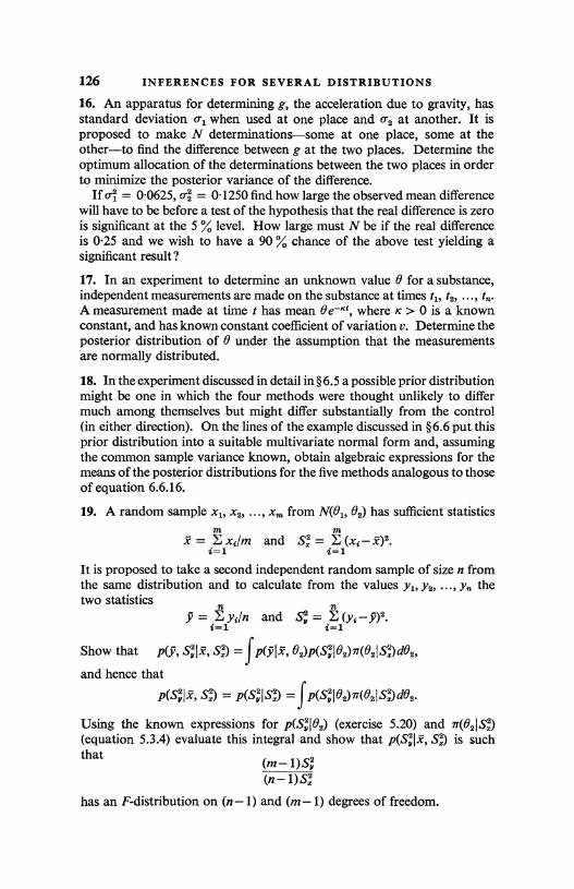
126 INFERENCES FOR SEVERAL DISTRIBUTIONS
16. An apparatus for determining g, the acceleration due to gravity, hasstandard deviation vl when used at one place and 02 at another. It isproposed to make N determinations-some at one place, some at theother-to find the difference between g at the two places. Determine theoptimum allocation of the determinations between the two places in orderto minimize the posterior variance of the difference.
If vi = 0.0625, (T2 = 0.1250 find how large the observed mean differencewill have to be before a test of the hypothesis that the real difference is zerois significant at the 5 % level. How large must N be if the real differenceis 0.25 and we wish to have a 90 % chance of the above test yielding asignificant result?
17. In an experiment to determine an unknown value 0 for a substance,independent measurements are made on the substance at times t1, t2, ..., t,,.A measurement made at time t has mean Oe Kt, where K > 0 is a knownconstant, and has known constant coefficient of variation v. Determine theposterior distribution of 0 under the assumption that the measurementsare normally distributed.
18. In the experiment discussed in detail in § 6.5 a possible prior distributionmight be one in which the four methods were thought unlikely to differmuch among themselves but might differ substantially from the control(in either direction). On the lines of the example discussed in §6.6 put thisprior distribution into a suitable multivariate normal form and, assumingthe common sample variance known, obtain algebraic expressions for themeans of the posterior distributions for the five methods analogous to thoseof equation 6.6.16.
19. A random sample x,, x2, ..., x,,, from N(01i 02) has sufficient statisticsm m
x = E x;/m and SS = E (x{-x)2.i=1 i=1
It is proposed to take a second independent random sample of size n fromthe same distribution and to calculate from the values y,, Y2, ..., y thetwo statistics n n
Y = iI ydn and Sy = iEi Yi -Y)2.
Show that p(Y, S,' 19, Si) = fP(PIx, 02)P(Svl BJ7T(02!Sz)d02,
and hence that
P(S;1x,SD =P(S"ISz) = f P(SYI0.1T(02ISz)dO2.
Using the known expressions for p(S102) (exercise 5.20) and 7r(02jSs)(equation 5.3.4) evaluate this integral and show that p(Sy19, Ss) is suchthat (m-1)Sn
(n-1)Sz
has an F-distribution on (n-1) and (m-1) degrees of freedom.
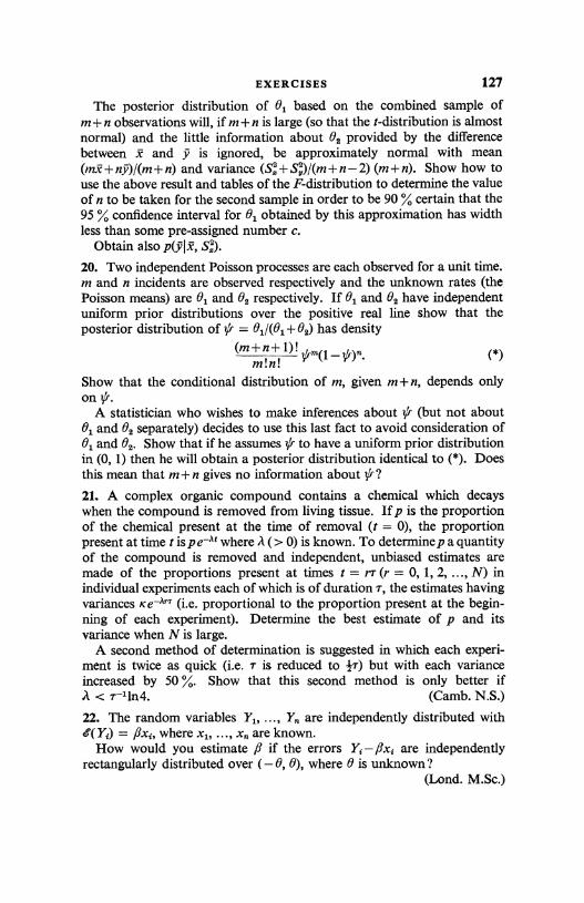
EXERCISES 127
The posterior distribution of 01 based on the combined sample ofm + n observations will, if m + n is large (so that the t-distribution is almostnormal) and the little information about 02 provided by the differencebetween x and y is ignored, be approximately normal with mean(mx+n9)/(m+n) and variance (m + n). Show how touse the above result and tables of the F-distribution to determine the valueof n to be taken for the second sample in order to be 90 % certain that the95 % confidence interval for 01 obtained by this approximation has widthless than some pre-assigned number c.
Obtain also p(ylx, SS).
20. Two independent Poisson processes are each observed for a unit time.m and n incidents are observed respectively and the unknown rates (thePoisson means) are 01 and 02 respectively. If 01 and 02 have independentuniform prior distributions over the positive real line show that theposterior distribution of VP = 01/(01+02) has density
(m + n + 1) !1//m(1- i/r)°. (*)
M! n!
Show that the conditional distribution of m, given m+n, depends onlyon.
A statistician who wishes to make inferences about ?f (but not about01 and 02 separately) decides to use this last fact to avoid consideration of01 and 02. Show that if he assumes ?r to have a uniform prior distributionin (0, 1) then he will obtain a posterior distribution identical to (*). Doesthis mean that m + n gives no information about ?/r?
21. A complex organic compound contains a chemical which decayswhen the compound is removed from living tissue. If p is the proportionof the chemical present at the time of removal (t = 0), the proportionpresent at time t is pelt where A (> 0) is known. To determinep a quantityof the compound is removed and independent, unbiased estimates aremade of the proportions present at times t = rr (r = 0, 1, 2, ..., N) inindividual experiments each of which is of duration T, the estimates havingvariances Kel- (i.e. proportional to the proportion present at the begin-ning of each experiment). Determine the best estimate of p and itsvariance when N is large.
A second method of determination is suggested in which each experi-ment is twice as quick (i.e. r is reduced to #T) but with each varianceincreased by 50 %. Show that this second method is only better ifA < T-11n4. (Camb. N.S.)
22. The random variables Y1, ..., Y. are independently distributed with,f(Y{) = ,Jx;, where x1, ..., x are known.
How would you estimate ft if the errors Y;-fix, are independentlyrectangularly distributed over (-0, 0), where 0 is unknown?
(Lond. M.Sc.)
128
7
APPROXIMATE METHODS
The results obtained for normal distributions in the two previouschapters were exact for the specified prior distribution. Indealing with samples for distributions other than normal it isoften necessary to resort to approximations to the posteriordensity even when the prior distribution is exact. In this chapterwe shall mainly be concerned with binomial, multinomial andPoisson distributions, but begin by describing an approximatemethod of wide applicability.
7.1. The method of maximum likelihoodLet x be any observation with likelihood function p(x I e)
depending on a single real parameter 0. The value of 0, denotedby O(x), or simply 0, for which the likelihood for that observa-tion is a maximum is called the maximum likelihood estimate of 0.Notice that 8 is a function of the sample values only: it is anexample of what we have previously called a statistic (§5.5).The definition generalizes to a likelihood depending on severalparameters p(x 1011 02, ..., B8) : the set (bl, 02i ..., 88) for whichthe likelihood is a maximum form the set of maximum likeli-hood estimates, 8i, of 0, (i = 1, 2, ..., s). The estimate is parti-cularly important in the special case where x = (x1, x2i ..., xn)is a random sample of size n from a distribution with density
f(xi 16). Then np(x 161) = rl f(xi 16).
4=1(1)
In this case the logarithm of the likelihood can be written asa sum: n
L(x 16) = lnp(x 18) _ lnf(xi 10). (2)i=1
Important properties of the log-likelihood, L(x 16), can bededuced from the strong law of large numbers (theorem 3.6.3)in the following way. In saying that x is a random sample we
7.1] THE METHOD OF MAXIMUM LIKELIHOOD 129
imply that the sample values have the same density f(xi 10) forsome 0 fixed, for all i. Denote this value of 0 by 00. We refer toit as the true value of 0. It is, of course, unknown. Then, foreach 0, the quantities, lnf(xi 10), are independent random vari-ables with a common distribution, depending on 00, and, by thestrong law, their mean converges strongly to their commonexpectation. By definition this expectation is
f o{ln f(xi I 9)} = f In f(xi 10). f(xi I Bo) dxi, (3)
where the suffix has been added to the expectation sign toindicate the true value, 0 i of 0. Hence the law says that withprobability one
lim {n-'L(x 161)} = So{In f(xi I 0)}. (4)n-*oo
Similarly, provided the derivatives and expectations exist,
lim {n-' l L(x I 0)/aor} = eo{or Inf(xi I 0)/90r}. (5)n-*m
Equation (4) may be expressed in words by saying that, forlarge n, the log-likelihood behaves like a constant times n, wherethe constant is the expectation in (3). Similar results apply inthe case of several parameters.
Theorem 1. If a random sample of size n is taken from f(xi 0)then, provided the prior density, ir(B), nowhere vanishes, theposterior density of 0 is, for large n, approximately normal withmean equal to the maximum likelihood estimate and variance, ten,,given bye'
ftft
Qn 2 = - a2L(x I v)/ao2. (6)
It is not possible to give a rigorous proof of this theorem at themathematical level of this book. The following `proof' shouldconvince most readers of the reasonableness of the result.
The posterior density is proportional toexp {L(x j0) +ln7r(0)},
and since we have seen that L(x 6) increases like n, it will ulti-mately, as n -> oo, dwarf Inn(B) which does not change with n.Hence the density is, apart from a constant, approximately
exp {L(x I B)} = exp{L(x 0) +3(0 - 0)202L(x 18)/ao2+ R},t a2L(x I B)/a02 denotes the second derivative with respect to 0 evaluated at B.
9 LS II
130 APPROXIMATE METHODS [7.1
on expanding L(x 10) by Taylor's theorem about 0, where R isa remainder term. Since the likelihood, and hence the log-likelihood, has a maximum at 0 the first derivative vanishes there.Also the second derivative will be negative there and may there-fore be written - acn 2. Furthermore, since it does not involve 0,the first term may be incorporated into the omitted constant ofproportionality and we are left with
exp { - 4(0 - 0)2/o 2 + R}. (7)
From the discussions of the normal density in §2.5 it is clearthat the term exp { - 1(0-#)2/0-1 } is negligible if 1 0 - 01 > 3o-n; sothat since o-; 2 is, by (5), of order n, this term is only appreciableif 0 differs from 0 by something of the order of n-I. In that casethe remainder term, R, which may be written
(B - 0)3 03L(x 1 OJ1003
for some 01, is of order n4 times n (by (5)). Hence it is of ordern_I and is negligible compared with the other term in (7).
Hence, inserting the constant of proportionality, the posteriordensity is approximately
.1, (8)(2nrT.)-l exp { - 4(9 - #)2/01
which establishes the result. Notice that o is, under the assump-tions made here, of order n-1.
Theorem 2. If a random sample of size n is taken from
f(xs 101, 02, ..., 0s)
then, provided the joint prior density, 7r(01i 02, ..., 0S) nowherevanishes, the joint posterior density is, for large n, approximatelymultivariate normal with means equal to the maximum likelihoodestimates B, and a dispersion matrix whose inverse has typicalelement - a2L(x 181, 82, , u3 Q)/ae. a0.. (9)
This is the extension of theorem 1 to the case of several para-meters. The proof proceeds as in that case. The important termsin the Taylor series expansion of L(x 1 0l, 02, ..., 03) are
8
2E (0,-0)
(e;-0)a2L(xI81, 02, ..., 08)/a0; 00J, (10)a
1
7.11 THE METHOD OF MAXIMUM LIKELIHOOD 131
and a comparison with the multivariate normal density (equa-tion 3.5.17) establishes the result.
The matrix, whose typical element is given by (9), will becalled the information matrix. It is the inverse of the dispersionmatrix of the posterior density (compare the definition ofprecision in §5.1). Similarly (6) is called the information.
General remarksAlthough known to earlier writers, the method of maximum
likelihood has only become widely used through the work ofR. A. Fisher, who obtained its principal properties. The mainadvantages of the method are that it produces a descriptionof the posterior distribution which, because it is normal, iseasy to handle, and which has a particularly simple mean andvariance. (We shall see below that these are easy to compute.)Fisher used the method to provide a point estimate of 0. Weshall not have much to say in this book about the problem ofpoint estimation; by which is usually meant the problem offinding a single statistic which is, in some sense, near to the truevalue of a parameter (see §5.2); our reason for not doing so isthat posterior distributions cannot be adequately described byone statistic. t But the problem is much discussed by somestatisticians and, in large samples, is adequately solved by themaximum likelihood estimate, though other approximations areavailable. There is, as we shall see below, a close relationshipbetween 92(6) and o-n above: so that 0 and its variance doprovide, because of the normality, an adequate description, inlarge samples, of the posterior density.
In the definition of 0 the word `maximum' is used in the senseof `largest value' : that is, L(x 10) >, L(x 0) for all 0. The esti-mate is therefore not necessarily determined by equating thefirst derivative to zero. This latter process will only yield thelocal maxima (or minima). An example where this process isinapplicable is provided by the uniform distribution discussedbelow. (In the `proof' it has been assumed that the first deriva-tive is zero at the maximum.)
t If we wished to use a single statistic we could take the mean of the posteriordistribution. But this would not be helpful without, in addition, at least thevariance.
9-2
132 APPROXIMATE METHODS [7.1
Notice that the method has little or nothing to recommend itin small samples. There are two reasons for this. First, theposterior distribution is not necessarily normal. Secondly, theprior distribution is relevant in small samples because the infor-mation provided by it may be comparable with the informationprovided by the sample, and any method based on the likelihoodalone may be misleading. We have mentioned the diminishingimportance of the prior distribution as the sample size increasesin connexion with the normal distribution (§§5.1, 5.2) but thepoint is quite general. Of course, if the prior knowledge is veryvague (as in theorem 5.2.1), even a small sample may containvirtually all the information. Notice that, in the statement ofthe theorems, it has been necessary to assume that the priordensity nowhere vanishes. If it did vanish near 01, say, then noamount of evidence would ever convince one that 0 was near 01(cf. § 5.2) and the posterior density would vanish near 01 even if0 = 01. (In the proof lnnr(0) would be minus infinity, andcertainly not negligible.)
Example: normal distribution
We begin with situations already studied, in order to see howthe approximation compares with the exact result. In the caseof the normal mean (§§5.1, 5.2) with known variance the likeli-hood is given by equation 5.1.9. The log-likelihood is therefore
L(x 10) = C - J(x - 0)2 (n/o.2),
where C is a constant. Differentiating and equating to zerogives the result (x - 0) (n/o2) = 0, so that 0 = X. A seconddifferentiation gives
R /Qn 2 = - a2L(x 10)/002 = (n/o2),
so that the posterior density is approximately N(x, 0-2 In), whichagrees with theorem 5.2.1, and is exact (corollary to theorem5.1.1) if the prior distribution of 0 is uniform over the real line.
If the variance is also unknown (§5.4) then the logarithm ofthe likelihood is, from equation 5.4.3 rearranged in the sameway as the posterior distribution was rearranged to obtain 5.4.4,
C - jn 1n 02 - {VS2 + n(x - 01)2}/202.
7.11 THE METHOD OF MAXIMUM LIKELIHOOD 133
To obtain the maximum likelihood estimates we differentiatepartially with respect to 01 and 02 and equate to zero. Theresults are
eL = n(x - 0,001
oL - - In + {vs2+n(x v2 = 0802 2 / 2 - #,)2}/2
2
so that 01 = x and #2 = VS2/n = E(x1-x)2/n. (12)
The matrix whose elements are minus the second derivatives ofthe log-likelihood at the maximum (the information matrix of(9)) is easily seen to be (nO_i 0 )
0 11n/02 13( )'
with inverse(020/n 202/n)
(14)2
The posterior distribution of 01 is thus approximately N(01i 62/n),or, from (12), nf(01-x)/s(v/n)1 is approximately N(0, 1). Thisis in agreement with the exact result (theorem 5.4.1) that0(01 -x)/s has Student's distribution, since this distributiontends to normality as n --> oo (§ 5.4), and v/n -> 1. The distribu-tion of 02 is approximately N(02, 2021n). This agrees with theexact result (theorem 5.4.2) that vs2/02 is x2 with v degrees offreedom, because the mean and variance of 02 are S2 and 2s4/v(equations 5.3.5 and 6) in large samples and the distribution of02 tends to normality. This last result was proved in § 5.3.Finally we note that the covariance between 01 and 02 is zero,which is in exact agreement with the result obtained in § 5.4.
Example: binomial distributionConsider a random sequence of n trials with constant proba-
bility 0 of success. If r of the trials result in a success thelikelihood is (cf. equation 5.5.9)
0*(1-0)n-. (15)
The derivative of the log-likelihood is therefore
r/0-(n-r)/(1-0),
134 APPROXIMATE METHODS [7.1
so that 0 = r/n, the proportion of successes in the n trials. Thesecond derivative is
- r/02 - (n - r)l(1 - 0)2,
which gives 0-n = r(n - r)/n3. These results agree with the exactresults of § 7.2.
Example: exponential family
The method of maximum likelihood is easily applied to anymember of the exponential family. In the case of a single suf-ficient statistic for a single parameter the density is (equation5.5.5)
f(xi 10) = F(xi) G(B) eu i>0ce>
and the log-likelihood is, apart from a constant,
ng(0) + t(x) 0(0),
nwhere g(O) = In G(0) and t(x) _ u(xi). The posterior densityi-iof 0 is therefore approximately normal with mean equal to theroot of
ng'(e) + t(x) ¢'(6) = 0 (16)
and variance equal to
{ - ng" (B) - t(x) 0"(0)}-1
evaluated at that root. Similar results apply in the case ofseveral sufficient statistics and parameters.
Solution of maximum likelihood equation
The equation for the maximum of the likelihood,
8L(x 10)/00 = 0,
or, in the case of the exponential family, (16) above, may not besolvable in terms of elementary functions. However, there is anelegant numerical method of solving the equation, in the courseof which vn is also obtained. This is Newton's method ofsolving an equation. A reference to fig. 7.1.1 will explain theidea. On a graph of the derivative of the log-likelihood against0 a tangent to the graph is drawn at a first approximation, 0(1),
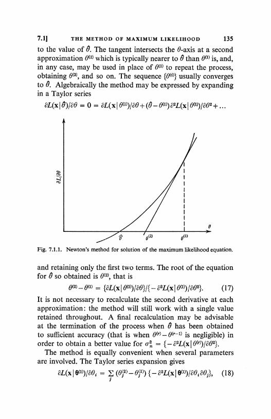
7.1] THE METHOD OF MAXIMUM LIKELIHOOD 135
to the value of 0. The tangent intersects the 0-axis at a secondapproximation 0(2) which is typically nearer to & than 0) is, and,in any case, may be used in place of 0(1) to repeat the process,obtaining 00, and so on. The sequence {0()} usually convergesto 0. Algebraically the method may be expressed by expandingin a Taylor series
3L(x10)/a0 = 0 = aL(xI0('))/aO+(0-e('>)a2L(xI e(1>)/002+...
0
Fig. 7.1.1. Newton's method for solution of the maximum likelihood equation.
and retaining only the first two terms. The root of the equationfor 6 so obtained is 00, that is
0(2)-0(1) = {aL(x 10('))/aO}/{ - a2L(x 10(l)) /0e2}. (17)
It is not necessary to recalculate the second derivative at eachapproximation : the method will still work with a single valueretained throughout. A final recalculation may be advisableat the termination of the process when 0 has been obtainedto sufficient accuracy (that is when 0 - 0(r-1) is negligible) inorder to obtain a better value for a-n = { - a2L(x j 0(r))/002}.
The method is equally convenient when several parametersare involved. The Taylor series expansion gives
aL(x 1 6(1))/80, = (0f2> - 0$')) {- a2L(x A°1>)/a0 a0jj, (18)
136 APPROXIMATE METHODS [7.1
where 0(1) = (011), 0(21), ..., 051)), a set of linear equations for0(2) - 84>. The matrix which has to be inverted is the informa-tion matrix at argument 64> instead of at argument 6. At thefinal approximation, 0(r), this has to be inverted in any case inorder to obtain the dispersion matrix. Thus the method is wellsuited, not only to the evaluation of the means, but also to theevaluation of the dispersion matrix, of the posterior distribu-tion. Numerical methods for the inversion of matrices are givenin § 8.4.
Example
As an illustration of Newton's method consider randomsamples from a r-distribution, or equivalently a x2-distribution,
with both the index and the parameter unknown. The densityfor a single observation is (equation 2.3.7)
Ba
.f(xi 101, 02) = (02011) ! e-xie3Lxia I, (19)
where we have written 01 for A and 02 for n. The likelihood fora random sample of size rn is thus
(02
018 )n exp j - 01 E xi + (02 -1) E In xi) . (20)- 1)! t i=1 i=1
JJ
This shows that the distribution belongs to the exponentialfamily and that x = Exi/n and y = E In xi/n are jointly sufficientstatistics. Differentiation of the log-likelihood gives
:n(-x+#2/QQ"1) = 0,a 01
802:n(lnO1+y-d021n(#2-1)!} _
(21)
The first of these equations is sufficiently simple to enable 81 tobe eliminated and a single equation,
ln62-lnx+y-d ln(92-1)! = 0, (22)2
for 82 to be solved by Newton's method. The derivative of theleft-hand side of (22) is 821- (d2/d02) In (O2 -1) ! and tables of thederivatives of the logarithm of the factorial function (see, for
7.1] THE METHOD OF MAXIMUM LIKELIHOOD 137
example, Davis (1933)) enable the calculations to be carried out.It is necessary, however, to start with a first approximation.Here this is most easily obtained by using the approximationtto d In (02 -1) !/d02 of 1n02 - 1/202, which, on insertion in (22),gives a value of 02 equal to {2(lnx-y)}-1 to use as 021> in theiteration. The approximation is remarkably good for all valuesof 02 except those near zero, so that except in that case, a singlestage of Newton's procedure should be sufficient. We leave thereader to verify that the dispersion matrix is the matrix
2
WO-2In (02 -1) ! 011
23O8i 1 82/82
with each element divided by n81 2{82d21n(82-1)!/d02-1}.These results might be of value if one wished to investigate
whether observed incidents were occurring in a Poisson process(§2.3). It might be reasonable to suppose the intervals betweensuccessive incidents to be independent (for example if the inci-dents were failures of a component which was immediatelyreplaced by a new one when it failed, §4.4), with a distributionof P-type. The Poisson process is the case 02 = 1(theorem 2.3.2),so one could perform an approximate significance test of thenull hypothesis that 02 = 1 by remarking that the posteriordistribution of 02 is approximately normal with mean 02 andvariance {n(d21n (02 -1)! /d02 - 821)}-1 = o-n, say. The approxi-mation to d2ln (02 -1) !/d02 of (1/02) + (1/20D, obtained from theabove approximation to the first derivative by another differ-entiation of Stirling's formula, shows that o is approximately282/n. The result will therefore be significant at the 5 % level if02 exceeds 1 + 2o- . Notice that, in agreement with the generalresult, o n is of the order n-1.
Choice of parameter
In the method of maximum likelihood there is no distinctionbetween the estimation of 0 and the estimation of a functionof 0, 0(0). We have the obvious relation that $ = 0(0). The
t This may be obtained by taking logarithms and differentiating both sides ofStirling's formula, equation 4.4.15.
138 APPROXIMATE METHODS [7.1
variance of ¢, {- 02L(x I )/aO2}-1, may also be related to the vari-ance of 0 in the following way. Write L for the log-likelihood inorder to simplify the notation. Then
aL aL dO a2L a2L (dolt aL d20V0 = 00 do
and a,2 a02 do-) + ae do-,
so that, since aL/00 = 0 at U, the second equation gives
-9201 X) _(dc5)I
912(01 X), (24)
where the derivative is evaluated at the maximum likelihoodvalue. These results may also be obtained from theorem 3.4.1since the variances are small, being of order n-1. Thus inchanging from 0 to 0 the means and variances change in theusual approximate way. Since the method does not distinguishbetween 0 and 0, both parameters have an approximatelynormal distribution. At first glance this appears incorrect sinceif 0 is normal then, in general, 0 will not be normal. But itmust be remembered that these results are only limiting ones asn --> oo and both the distributions of 0 and 0 can, and indeed do,tend to normality. What will distinguish 0 from 0 in this respectwill be the rapidity of approach to normality: 0 may be normalto an adequate approximation for smaller n than is the casewith 0. It often pays, therefore, to consider whether some trans-form of 0 is likely to be more nearly normal than 0 itself and,if so, to work in terms of it. Of course, there is some transformof 0 which is exactly normal since any (sufficiently respectable)distribution can be transformed into any other (compare theargument used in §3.5 for obtaining random samples from anydistribution), but this transform will involve the exact posteriordistribution and since the point of the approximation is toprovide a simple result this is not useful. What is useful is to takea simple transformation which results in a more nearly normaldistribution than is obtained with the untransformed para-meter. No general results seem available here, but an exampleis provided by the variance 02 of a normal distribution just dis-cussed. The distribution of 02, as we saw in § 5.3, has a longertail to the right (large 02) than to the left (small 02). This suggestsconsidering In 02 which might remove the effect of the long tail.
7.11 THE METHOD OF MAXIMUM LIKELIHOOD 139
Detailed calculations show that the posterior distribution ofln02 is more nearly normal than that of 02, though even bettertransformations are available. The approximate mean and vari-ance of the distribution of In 02 may be found either by maximumlikelihood directly, equation (9), or from the results for 02,equation (14), combined with equation (24). Other exampleswill occur in later sections.
Distribution of the maximum likelihood estimateWe saw in §5.1 that when making inferences that involved
using the mean of a normal distribution there were two distinctresults that could be confused (statements (a) and (b) of thatsection). A similar situation obtains here because of theapproximate normality of the posterior distribution. The twostatements are :
(a) the maximum likelihood estimate, 0, is approximatelynormally distributed about 00 with variance the inverse of
In(0o) = eo{ - l 2L(X I Oo)/1302}; (25)
(b) the parameter 0 is approximately normally distributedabout 0 with variance an.
(0o is the true, unknown, fixed value of 0 as explained before,equation (3).) Statement (b) is the result of theorem 1, state-ment (a) can be proved in essentially the same way as that theoremwas proved. Statement (a) is a result, in frequency proba-bility, about a statistic, 0: (b) is a result, in degrees of belief,about a parameter 0. In practice (a) and (b) can be confused,as explained in §5.1, without harm. Actually (a) is rarely usedin the form given, since 0o is unknown and yet occurs in thevariance (equation (25)). Consequently, (25) is usually replacedby In(0). This still differs from vn 2 because of the expectationtused in (25) but not in the expression for cn2. It is interestingto note that the use of the expectation makes no difference inrandom samples of fixed size from an exponential family: thereIn(0) = cc 2. (See equation (16) and the one immediatelyfollowing.)
t Those who have read the relevant paragraph in § 5.6 will notice that the useof the expectation violates the likelihood principle, and is, on this score, unsatis-factory.
140 APPROXIMATE METHODS [7.1
Exceptional casesIt is necessary to say a few words about the question of rigour
in the proofs of the theorems. A complete proof with all thenecessary details is only possible when certain assumptions aremade about the likelihood: for example, assumptions about theexistence and continuity of derivatives and their expectations.These assumptions are not always satisfied and the theorem isnot always true; the most common difficulty arises when therange of possible values of xi depends on 0. The difficulty is thesame as that encountered in discussing sufficiency in §5.5 andthe same example as was used there suffices to demonstrate thepoint here. If I
and is otherwise zero; then the likelihood is 0-n provided0 > max x2 = X, say, and is otherwise zero. Hence the
iposterior density is approximately proportional to 0-n andclearly this does not tend to normality as n -+ oo. Indeed, themaximum value is at 0 = X, so that 0 = X, at the limit of therange of values of 0 with non-zero probability. If the priordistribution of 0 is uniform over the positive half of the realline, a simple evaluation of the constant shows that
7T(6 I x) = (n - 1) Xn-10-n (0 > X, n > 1),
with mean (n - 1) X/(n - 2) and variance (n - 1) X2/(n - 3) (n - 2)2if n > 3. As n --> oo the variance is approximately X2/n2, whereasthe theorem, if applicable here, would give a result that is oforder n-1, not n-2. The estimation of 0 is much more accuratethan in the cases covered by the theorem. The practical reasonfor the great accuracy is essentially that any observation, xi,immediately implies that 0 < xi has zero posterior probability;since, if 0 < xi, xi has zero probability. This is a much strongerresult than can usually be obtained. The mathematical reasonis the discontinuity of the density and its differential withrespect to 0 at the upper extreme of the range of x. Difficultiescan also occur with estimates having smaller accuracy than sug-gested by the theorem, when dealing with several parameters.Examples of this phenomenon will not arise in this book.
7.21 RANDOM SEQUENCES OF TRIALS 141
7.2. Random sequences of trialsIn this section we consider the simple probability situation of
a random sequence of trials with constant probability, 0, ofsuccess, and discuss the inferences about 0 that can be made.If a random variable, x, has a density
(a+ b+ 1)!,a! b!
for 0 5 x 1 and a, b > - 1, it is said to have a Beta-distribu-tion with parameters a and b. We write it Bo(a, b), the suffixdistinguishing it from the binomial distribution B(n, p) withindex n and parameter p (§2.1).
Theorem 1. If, with a random sequence of n trials with constantprobability, 0, of success, the prior distribution of 0 is Bo(a, b),then the posterior distribution of 0 is Bo(a+r, b + n - r) where r isthe number of successes.
The proof is straightforward:
71(0) cc 9a(1-6)b, from (1), (2)
the likelihood is p(x 10) = 0 (l - 0)71-,
so that 1T(0 I x) oc 0a+r(l -0)b+n-r, (3)
proving the result. (Here x denotes the results of the sequenceof trials. Since r is sufficient 7r(0 I x) maybe written 9r(01r).)Corollary 1. Under the conditions of the theorem the posteriordistribution of
(4)1 0a+r+ -
is F[2(a+r+ 1), 2(b+n-r+ 1)].
From (4) dF/dO oc (1-0)-2
and also 0 = a'F/(b'+a'F),
where a' = a + r + 1, b' = b + n - r + 1. Substitution in (3), notforgetting the derivative (theorem 3.5.1), gives
7r(Fj x) oc Fa'-1/(b' +a'F)a+b'
oc Fa'-1/(2b' + 2a'F)a +b'.
1
b+n-r+F
( )V
xa(l -x)b (1)
142 APPROXIMATE METHODS [7.2
A comparison with the density of the F-distribution (equation6.2.1) establishes the result.Corollary 2. The posterior distribution of In {8/(1- B)} has, forlarge r and (n - r), approximate mean
a+2-b+r,In{r/(n-r)}+r n-r(5)
rid 1 1 (6)an va ance +r (n - r)'
In § 6.2 the mean and variance of the F-distribution wereobtained. From those results and corollary 1, the mean of F,given by equation (4), is
b+n-r+l 1 1
b+n-r 1 +b+n-r 1 +n-r (7)'
and the variance is approximately n/r(n - r). Since the varianceof F is small when r and (n - r) are large, the mean and varianceof u = In F can be found to the same order of approximation asin (7) by use of theorem 3.4.1.
&(u) A In (1 +1 n
n-r 2r(n-r) (1 +n-r)1 _ n =1 1 _1 (8)
n-r 2r(n-r) 2 n-rr,
-2
and _92(u)(1+1 n - 1 +1 . (9)n-r r(n-r) r n-r
Since u = In{(b+n-r+1)/(a+r+1)}+In{e/(1- e)} the expres-sion, (6), for the variance immediately follows. That for themean, (5), is easily obtained since
.°{ In [6/(1- 0)]} 6'(u) + In {(a + r + 1)/(b + n - r + 1)}
1 1 1+ In
r +a+1 b+l2 n-r r n-r r n-r
= Inr +a+jb+jn-r r n-r
7.2] RANDOM SEQUENCES OF TRIALS 143
Beta-distribution
The family of Beta-distributions is convenient for randomvariables which lie between 0 and 1. An important property ofthe family is that y = 1 - x also has a Beta-distribution, but witha and b interchanged, that is B0(b, a). This is obvious from thedensity. This makes it particularly useful if x is the probabilityof success, for y is then the probability of failure and has a dis-tribution of the same class. That the integral of (1) is unityfollows from the Beta-integral (equation 5.4.7). The sameintegral shows that the mean is (a + l)/(a + b + 2) and the vari-ance (from equation 2.4.5) is
(a+l)(a+2) _ (a+l)2 _ (a+l)(b+l) (10)(a+b+2) (a+b+3) (a+b+2)2 (a+b+2)2 (a+b+3)'
If a and b are positive the density increases from zero at x = 0to a maximum at x = a/(a+b) and falls again to zero at x = 1.If -1 < a < 0 or -1 < b < 0 the density increases withoutlimit as x approaches 0 or 1, respectively. The case of small aand large b corresponds to a distribution in which x is usuallynearer 0 than 1, because the mode and mean are then both nearzero. The relation between the Beta- and F-distributions hasalready been seen in deriving equation 6.2.5.
Change in Beta-distribution with samplingApart from the reasons just given, the family of Beta-distribu-
tions is the natural one to consider as prior distributions for theprobability 0 of success. We saw in § 5.5 that any member of theexponential family had associated with it a family of conjugateprior distributions (cf. equation 5.5.18). The likelihood herebelongs to the exponential family (equation 5.5.12) and theconjugate family is easily seen to be the Beta-family of distribu-tions. Theorem 1 merely expresses the result discussed afterequation 5.5.18 that the posterior distribution also belongs tothe same family but with different parameters. In fact a and bchange into a + r and b + (n - r). It is often convenient to repre-sent the situation on a diagram (fig. 7.2.1). The axes are of a andb. The prior distribution corresponds to the point (a, b) with, say,
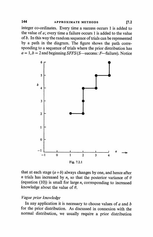
144 APPROXIMATE METHODS [7.2
integer co-ordinates. Every time a success occurs 1 is added tothe value of a; every time a failure occurs 1 is added to the valueof b. In this way the random sequence of trials can be representedby a path in the diagram. The figure shows the path corre-sponding to a sequence of trials where the prior distribution hasa = 1, b = 2 and beginning SFFS (S-success: F-failure). Notice
6
5
b4
3
2
1
0
-1 I 1 1 I a-1 0 1 2 3 4
Fig. 7.2.1
that at each stage (a + b) always changes by one, and hence aftern trials has increased by n, so that the posterior variance of 0(equation (10)) is small for large n, corresponding to increasedknowledge about the value of 0.
Vague prior knowledge
In any application it is necessary to choose values ofa and bfor the prior distribution. As discussed in connexion with thenormal distribution, we usually require a prior distribution
7.21 RANDOM SEQUENCES OF TRIALS 145
corresponding to a fair amount of ignorance about the para-meter. The situation where the prior knowledge of 0 is not vagueis discussed below. Since any observation always increaseseither a or b it corresponds to the greatest possible ignorance totake a and b as small as possible. For the prior density to havetotal integral 1 it is necessary and sufficient that both a and bexceed - 1. Therefore the usual prior distribution to take is thatwith a = b = - 1. It is true that the resulting density can onlybe defined as a conditional density, but we have already usedthis type of prior density in supposing the mean or log-varianceof the normal distribution to be uniformly distributed. In factthe density just suggested is proportional to {0(1 - 0)}-1: this isequivalent to saying that 0 = In{0/(1- 0)} is uniformly distri-buted over the whole real line, since do/dO = {0(1- 0)}-1. Hencethe convenient parameter to consider is 0, the logarithm of theodds in favour of the event of success in a trial. Notice that itis this parameter which occurs in the natural representation ofthe likelihood as a member of the exponential family (equa-tion 5.5.12). With a = b = -1 the posterior distribution isBo(r - 1, n - r - 1), the two parameters being one less than thenumber of successes and failures respectively. Bayes himselfsuggested supposing 0 to be uniformly distributed over theinterval (0, 1) and this distribution has often been suggested bylater writers; a common argument in its favour being that if weare ignorant of 0 then any value of 0 is as likely as any other.Unfortunately this argument also applies to ¢. The practicaldifference between these two apparently very different densitiesis, however, slight because two observations, one a success andone a failure, are sufficient to change one (c uniform) into theother (0 uniform). This is clearly seen from fig. 7.2.1.t So inarguing in favour of one against the other we are only arguingover the equivalent of two observations, usually a small fractionof the total number, n, of observations on which the posteriordistribution is based. If the uniform distribution of 0 is usedthen the posterior distribution can only be defined as a con-ditional density until both a success and a failure have beenobserved. It is not unreasonable to say that reliable inferences
t Notice that in the figure the axes pass through a = b = -1.10 LSII
146 APPROXIMATE METHODS [7.2
cannot be made about the ratio of successes to failures until anexample of each has occurred.
Use of F-tables
In order to reduce the number of tables of distribution func-tions that is needed, it is convenient in practice to use therelation between the Beta-distribution and the F-distribution anduse tables of the latter (compare the discussion at the end of§ 5.4). This is the purpose of corollary 1. With a = b = -1 thequantity having the F-distribution is
F (nrr) (l-0) \1-O)/ nrrl' (11)
the ratio of the odds in favour of success to the empirical oddsin favour of success; the empirical odds being the ratio ofobserved number of successes to number of failures. The degreesof freedom are 2r and 2(n - r) ; twice the numbers of successesand failures respectively. Confidence intervals for F are given inthe usual way (§6.2) with the F-distribution. A confidence in-terval for F of coefficient Q is given by
F = FIa [2r, 2(n - r)] < F < FIa [2r, 2(n - r)] = F,
with a = 1-f3. In terms of 0 this is equivalent to
rF/(n - r) < 6 < rF/(n - r) (12)1 + rF/(n - r) 1 + rF/(n - r)
Since F is not directly tabulated it is more convenient to useequation 6.2.7 and to write (12) as
where1 + (n
1
r) F'/r< 8 <
1 + (n 1 r)/rF '(13)
F' = FI2 [2(n - r), 2r] _ {FIa [2r, 2(n - r)]}-1 = F-1.
The limits given by (13) are wider than people usually expectand a numerical example may prove instructive. In 17 trials,5 successes (and 12 failures) were observed. The degrees of free-dom for F are therefore 10 and 24, so that F = 2.64 witha = 0.05, and F' = 3.37, from the tables. Hence (n - r)/rF = 0.91
7.21 RANDOM SEQUENCES OF TRIALS 147
and (n - r) F'lr = 8.09, so that the 95 Y. confidence interval for 0is, from (13), (0.11, 0.52). The mean value of the posterior dis-tribution is r/n, namely 0.29. Notice that the interval is notsymmetric about the mean, the upper value differing from it by0.23, but the lower only by 0.18. The interval is only symmetricwhen r = n - r, the mean then being 1.
Approximate methodsThe Beta- and F-distributions are a little awkward to handle,
especially when inferences are to be made on the basis of severalsamples, and it is desirable to develop suitable approximations.The maximum likelihood method of §7.1 provides one suchapproximation, and we saw in that section that the posteriordistribution of 0 was approximately N(r/n, r(n -r)ln3).and variance agree, in large samples, with the exact results, fromequation (10) above, of (a+r+l)/(a+b+n+2) and
(a+r+ 1) (b+n-r+ 1)/(a+b+n+2)2 (a+b+n+3),
but the approach to normality is slow unless r is about In.Thus in the numerical example the posterior distribution is,according to the approximation, and with a = b = -1,N(0.29, 0.0122), so that the 95 % confidence limits are (0-07,0-51),not in too good agreement with the exact result, especially at thelower limit. Notice that this interval, unlike the exact one, isnecessarily symmetrical about the mean. As explained in §7.1some parametric functions will have a more nearly normal dis-tribution than others and so we look for a better approximationusing a parameter different from 0. The F-distribution is nomore nearly normal than is the Beta-distribution, but since(§ 6.2), for all except very small values of the degrees of freedom,the density increases rapidly from zero at F = 0 to a maximumnear F = 1 and then decreases slowly to zero as F-k oo, it looksas though lnFwill be much more nearly normal. The logarithmwill have a stronger effect on the sharp left-hand tail, betweenF = 0 and F = 1, than on the right-hand tail, above F = 1.This transformation was first suggested by Fishert and lnFinaybe shown to have a normal distribution to a much better approxi-
j' Fisher took 4lnF, but the I is more conveniently omitted in this context.10-2
148 APPROXIMATE METHODS [7.2
mation than does F itself. The transformation also commendsitself in the present situation because In{0/(1- 0)}, which differsfrom In F by a constant, is the natural parameter to consider,both in the representation of the original distribution in expo-nential form (equation 5.5.12) and as the parameter having auniform prior distribution.
Corollary 2 gives the mean and variance of the posterior dis-tribution of In {6/(1- 0)}, as far as the terms in 1 /r and 1 /(n - r),which, in conjunction with the assumption of normality, aresufficient to define the posterior distribution. The logarithm isthe dominant term in the mean, the next term is of smaller orderand may be ignored for large r and (n - r) : in any case it is ofsmaller order than the standard deviation. Notice that the priordistribution only enters into this second term, and not into thedominant terms of mean and variance. This is another exampleof the fact that for large samples the prior distribution can beignored. Notice that, to the same order (5) may be written
Inr+a+4 (14){n-r+b+#}'
which is more convenient for calculation. Consider this approxi-mation in the numerical case just cited with n - r = 12 andr = 5, and a = b = - 1. The logarithm of the odds is approxi-mately normal with mean -0-939 and standard deviation0.532, and hence 95 % confidence limits are -1.982 and+0.104, giving 95 % confidence limits for 0 of (0.12, 0.53),agreeing very well with the exact values of (0- 11, 0.52) obtainedabove using the F-distribution.
Approximation to the likelihoodAnother method of obtaining a useful approximate result is
to approximate to the likelihood instead of to the posteriordistribution directly. In particular, if the likelihood can bechanged into an approximately normal one, then the inferencesappropriate to a normal distribution can be made. Now onereason why inferences for the binomial distribution are not assimple as for the normal is that the parameter of interest affectsboth mean and variance. It is therefore sometimes convenient
7.21 RANDOM SEQUENCES OF TRIALS 149
to find a transformation which will remove the parameter fromthe variance. We saw how this could be done in certain cases in§ 3.4. In particular for the binomial distribution (example 3 ofthat section), if r is B(n, p) then sin-14/(r/n) has approximatevariance 1 /4n, not dependent on p, about a mean of sin-1Jp.Furthermore, it may be shown that the distribution of theinverse-sine is more nearly normal than is that of r itself. Con-sequently, it is now possible to make inferences using the approxi-mate normality of sin-1V(r/n). The transformation is tabulatedin Lindley and Miller (1961) and in the numerical exampleabove, sin-14/(5/17) = 0.573 (in radians) with a standard devia-tion of 1 /V68 = 0.121. Hence 95 % confidence limits for theinverse sine are approximately 0.573 ± 1.96 x 0.121, that is(0.336, 0.810). Applying the inverse transformation the limitsfor 9 are (0- 11, 0.52) in agreement with the exact values.
The inverse-sine transformation is particularly valuablebecause it enables all the inference methods appropriate to thenormal distribution to be used with the binomial. For example,suppose we have k independent sets of random sequences eachof n trials, with constant probabilities of success O , and givingri successes (i = 1, 2, ..., k). Then xi = sin-1V(ri/n) will be ap-proximately normal with means sin-14/81 and common variance1 /4n. Consequently the hypothesis that the 6i's are all equal canbe tested by the analysis of variance method of § 6.4, usingtheorem 2 of that section, since the variance is known. The teststatistic will be 4n E(xi - x.)2, which may be approximately com-pared with a X2-distribution with (k -1) degrees of freedom.
A disadvantage of the inverse-sine transformation is that thetransform is not a useful parameter to consider. Thus, if wecarry out an analysis of variance as described in §8.5 on theinverse-sines and learn that an interaction is probably zero, thatresult is not usually of much value to the experimenter to whomthe inverse-sine is not a physically meaningful quantity.
The reader who has studied the final part of §5.6 may objectto the above argument since it uses the distribution of r toderive the transformation and not just the likelihood. This maybe avoided, however, by replacing the argument of example 3of § 3.4, by the comparable argument of §7.1 in connexion with
150 APPROXIMATE METHODS [7.2
maximum likelihood. Equation (24) of that section replacesequation 3.4.2 and the purpose of the transformation is to finda parameter about which the information is constant. Thisappears to have been Fisher's intention in producing the trans-formation originally.
Several samplesThe true worth of any of these approximations is only appre-
ciated when considering several samples. Suppose, for example,that we have two independent random sequences of n1 trials,with constant probability, 02, of success, yielding rj successes(i = 1, 2). Then we may wish to inquire about differencesbetween 01 and 02 and, in particular, to make a significance testof the hypothesis that 01 = 02. This hypothesis may be con-veniently rephrased in terms of the logarithms of odds byinvestigating 01- 02 = In {01(1- 02)/02(1- 0)} and, in particular,testing whether 01- 02 = 0. The posterior distributions of 01and 0h2 will be independent and both approximately normal,so that the posterior distribution of 01- ¢2 is approximatelynormal with mean
[r,(n2In (nl rl rl) -In (n2 - r2) = In
n
rlr2l1
(15)
and variance 1 + I + 1 + 1 (16)rl nl - r1 r2 n2 - r2
(In (15) the second term of (5) has been ignored, or equivalentlywe have supposed a = b = -1.) Hence the null hypothesisthat 01 = 02, or equivalently 01 = 02, will be judged significantat the 5 % level if (15) exceeds 1.96 times the standard deviationobtained from (16): that is, if
{rl(n2In
- r2) 2
(n1-rl)r2) > (1.96)2 = 3.84. (17)
(r,1
+n1 1 r1+rL+n2 i r2)This method may be extended to cover numerous other situa-tions but we shall not pursue it any further here since anothermethod, using a different approximation, is available and ismore commonly used. This will be studied in § 7.6.
7.2] RANDOM SEQUENCES OF TRIALS 151
Inference with appreciable prior knowledgeWe now consider the analysis suitable when the prior know-
ledge of 8 is comparable in its importance to the knowledge tobe obtained from the likelihood function. The situation we havein mind is exemplified by a problem concerning a defect in amass-produced model of a car. The parameter in question is theproportion of cars of this particular model exhibiting the defectby the time they are one year old. After the model had been inproduction about a year the manufacturer realized, from com-plaints received, that this defect was of reasonably commonoccurrence. He naturally wished to find out how common itwas and proposed to carry out a survey. For our purposes itwill suffice to suppose that the survey consists in taking a randomsample of size n of one-year-old cars and observing the number,r, with the defect. The likelihood will then be that considered inthis section. However, there is already, before the sample istaken, some knowledge of 8. It is difficult to be precise aboutthis because some customers will not notice the defect, otherswill not complain even if they do notice it, and not all complaintswill reach the group in the manufacturing company conductingthe investigation. Nevertheless, some information is availableand should be incorporated into the analysis.
The question is: how should the prior knowledge be obtainedand expressed? It will be most convenient if it is expressed interms of the Beta-distribution, should this be possible. In orderto do this it is necessary to obtain the values of a and b : whenthis has been done theorem 1 may be applied. In the examplethe company felt that the defect most probably occurred in about15 % of their cars, and that it must certainly occur in about 5 %in order to explain the complaints already received. They alsofelt it to be most unlikely that more than I in 3 of the cars wouldexhibit the defect. This information can be turned into a prob-ability density by supposing that the upper and lower limitsquoted correspond roughly to the upper and lower 5 % pointsof a Beta-distribution. From tables of the percentage points ofthis distribution (for example those in Pearson and Hartley(1958), Table 16) the values a = 2, b = 14 provide upper and
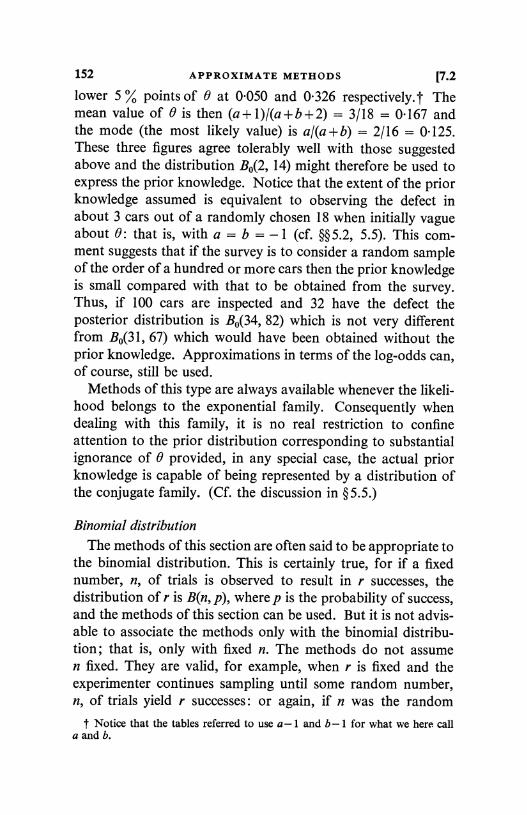
152 APPROXIMATE METHODS [7.2
lower 5 Y. points of 0 at 0.050 and 0.326 respectively. t Themean value of 0 is then (a+1)/(a+b+2) = 3/18 = 0.167 andthe mode (the most likely value) is a/(a+b) = 2/16 = 0.125.These three figures agree tolerably well with those suggestedabove and the distribution BO(2, 14) might therefore be used toexpress the prior knowledge. Notice that the extent of the priorknowledge assumed is equivalent to observing the defect inabout 3 cars out of a randomly chosen 18 when initially vagueabout 0: that is, with a = b = -1 (cf. §§5.2, 5.5). This com-ment suggests that if the survey is to consider a random sampleof the order of a hundred or more cars then the prior knowledgeis small compared with that to be obtained from the survey.Thus, if 100 cars are inspected and 32 have the defect theposterior distribution is B0(34, 82) which is not very differentfrom B0(31, 67) which would have been obtained without theprior knowledge. Approximations in terms of the log-odds can,of course, still be used.
Methods of this type are always available whenever the likeli-hood belongs to the exponential family. Consequently whendealing with this family, it is no real restriction to confineattention to the prior distribution corresponding to substantialignorance of 0 provided, in any special case, the actual priorknowledge is capable of being represented by a distribution ofthe conjugate family. (Cf. the discussion in §5.5.)
Binomial distribution
The methods of this section are often said to be appropriate tothe binomial distribution. This is certainly true, for if a fixednumber, n, of trials is observed to result in r successes, thedistribution of r is B(n, p), where p is the probability of success,and the methods of this section can be used. But it is not advis-able to associate the methods only with the binomial distribu-tion; that is, only with fixed n. The methods do not assumen fixed. They are valid, for example, when r is fixed and theexperimenter continues sampling until some random number,n, of trials yield r successes : or again, if n was the random
t Notice that the tables referred to use a-1 and b-1 for what we here calla and b.
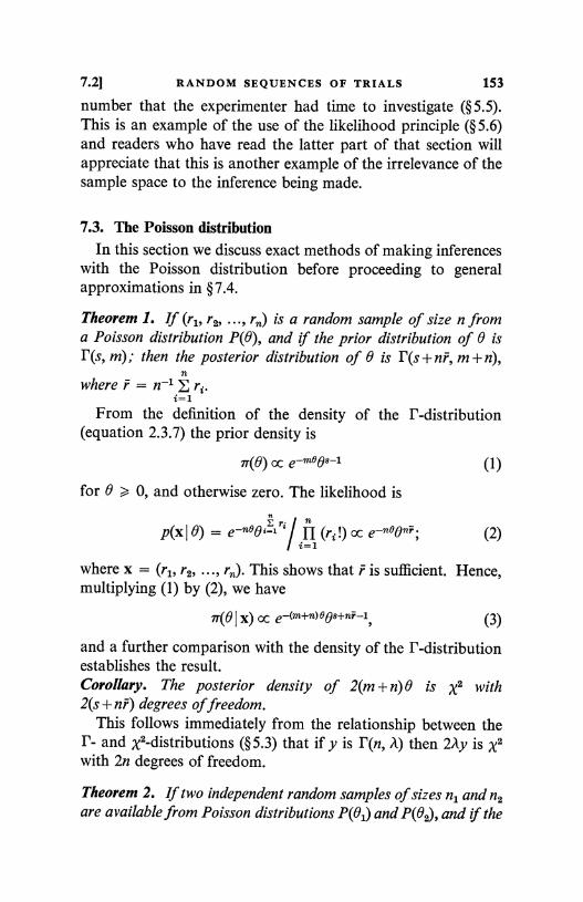
7.2] RANDOM SEQUENCES OF TRIALS 153
number that the experimenter had time to investigate (§ 5.5).This is an example of the use of the likelihood principle (§5.6)and readers who have read the latter part of that section willappreciate that this is another example of the irrelevance of thesample space to the inference being made.
7.3. The Poisson distributionIn this section we discuss exact methods of making inferences
with the Poisson distribution before proceeding to generalapproximations in § 7.4.
Theorem 1. If (r1i r2, ..., rn) is a random sample of size n froma Poisson distribution P(O), and if the prior distribution of 0 isP(s, m); then the posterior distribution of 0 is P(s+nf, m + n),
where r = n-1 ri.i=1
From the definition of the density of the P-distribution(equation 2.3.7) the prior density is
1T(0) oc a-m90 -1 (1)
for 0 > 0, and otherwise zero. The likelihood is
l 1
n
0 ; (2)p(x 10) =e-noet£i'a
11 (r11) cc a-n° li=1
(2)
where x = (r1, r2, ..., rn). This shows that F is sufficient. Hence,multiplying (1) by (2), we have
7r(6I x) oc e-(m+n)o08+nT-1 (3)
and a further comparison with the density of the P-distributionestablishes the result.Corollary. The posterior density of 2(m +n) 0 is x2 with2(s + nF) degrees of freedom.
This follows immediately from the relationship between ther- and X2 -distributions (§5.3) that if y is P(n, A) then 2A1y is x2with 2n degrees of freedom.
Theorem 2. If two independent random samples of sizes n1 and n2
are available from Poisson distributions P(01) and P(02), and if the
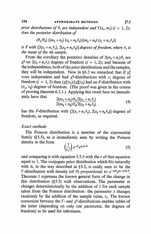
154 APPROXIMATE METHODS [7.3
prior distributions of Oi are independent and F(si, mi) (i = 1, 2);then the posterior distribution of
(e1/B2) {(m1 + n1) (s2 + n2 r2)/(m2 + n2) (s, + n1 F1))
is F with [2(s1 + n1 rl), 2(52 + n2 rr2)] degrees of freedom, where ri isthe mean of'the ith sample.
From the corollary the posterior densities of 2(mi+ni)Oi arex2 on 2(si+niri) degrees of freedom (i = 1, 2); and because ofthe independence, both of the prior distributions and the samples,they will be independent. Now in §6.2 we remarked that if xzwere independent and had X2-distributions with vi degrees offreedom (i = 1, 2) then (xi/vl)/(x2/v2) had an F-distribution with(v1, v2) degrees of freedom. (The proof was given in the courseof proving theorem 6.2.1.) Applying this result here we immedi-ately have that
2(m1 + n1) 61/2(sl + n1 r1)4()
2(m2 + n2) 02/2(52 + n2 r2)
has the F-distribution with [2(s1 +n1 F1), 2(S2+ n2 r2)] degrees offreedom, as required.
Exact methods
The Poisson distribution is a member of the exponentialfamily (§ 5.5), as is immediately seen by writing the Poissondensity in the form 1
(-I a-e eri In 0 (5)ri
and comparing it with equation 5.5.5 with the r of that equationequal to 1. The conjugate prior distribution which fits naturallywith it, in the way described in § 5.5, is easily seen to be theP-distribution with density (of 0) proportional to e-moe(8-1)lne
Theorem 1 expresses the known general form of the change inthis distribution (§5.5) with observations. The parameter mchanges deterministically by the addition of 1 for each sampletaken from the Poisson distribution: the parameters changesrandomly by the addition of the sample value, r.. The knownconnexion between the r- and X2 -distributions enables tables ofthe latter (depending on only one parameter, the degrees offreedom) to be used for inferences.
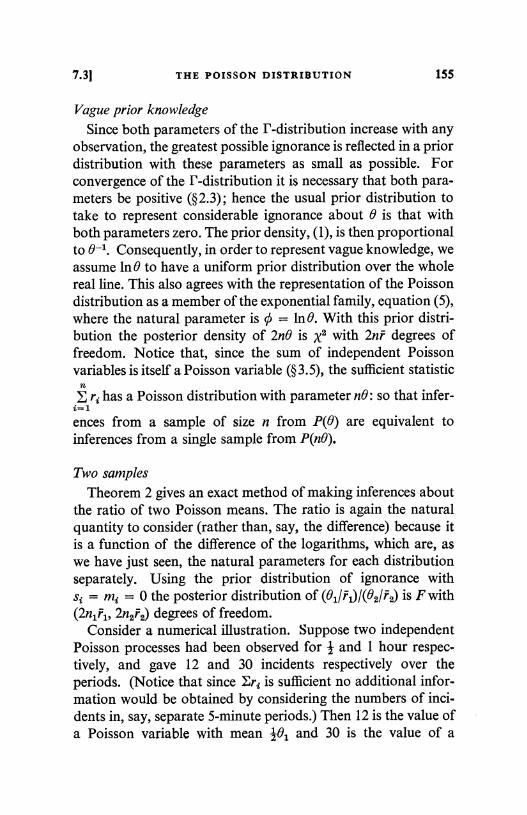
7.31 THE POISSON DISTRIBUTION 155
Vague prior knowledgeSince both parameters of the P-distribution increase with any
observation, the greatest possible ignorance is reflected in a priordistribution with these parameters as small as possible. Forconvergence of the 1-distribution it is necessary that both para-meters be positive (§2.3); hence the usual prior distribution totake to represent considerable ignorance about 0 is that withboth parameters zero. The prior density, (1), is then proportionalto 0-1. Consequently, in order to represent vague knowledge, weassume In 0 to have a uniform prior distribution over the wholereal line. This also agrees with the representation of the Poissondistribution as a member of the exponential family, equation (5),where the natural parameter is 0 = In 0. With this prior distri-bution the posterior density of 2n0 is x2 with 2nF degrees offreedom. Notice that, since the sum of independent Poissonvariables is itself a Poisson variable (§ 3.5), the sufficient statistic
nri has a Poisson distribution with parameter n0: so that infer-
ences from a sample of size n from P(0) are equivalent toinferences from a single sample from P(nO).
Two samplesTheorem 2 gives an exact method of making inferences about
the ratio of two Poisson means. The ratio is again the naturalquantity to consider (rather than, say, the difference) because itis a function of the difference of the logarithms, which are, aswe have just seen, the natural parameters for each distributionseparately. Using the prior distribution of ignorance withsi = mi = 0 the posterior distribution of (01/F1)/(02/F2) is F with(2n1F1i 2n2F2) degrees of freedom.
Consider a numerical illustration. Suppose two independentPoisson processes had been observed for I and 1 hour respec-tively, and gave 12 and 30 incidents respectively over theperiods. (Notice that since Eri is sufficient no additional infor-mation would be obtained by considering the numbers of inci-dents in, say, separate 5-minute periods.) Then 12 is the value ofa Poisson variable with mean 101 and 30 is the value of a
156 APPROXIMATE METHODS [7.3
Poisson variable with mean 02, where 01 and 02 are the rates ofoccurrence per hour of incidents in the two processes. It followsthat the posterior distribution of (101/12)/(02/30) is F with 24and 60 degrees of freedom (n1 = n2 = 1). The upper and lower22 % points of the F-distribution with those degrees of freedomare 1.88 and 0.48 respectively, so that a 95 % confidence intervalfor 01/02 is
(314o) 0.48 < 01/02 < (310) 1.88,
that is 0.38 < 01/02 < 1.50.
ApproximationsThe logarithmic transformation of F can be used, if the
F-tables are not available, with the approximate normality andmean and variance obtained as in the previous section.
The logarithmic transformation can be useful when handlingseveral Poisson distributions, though the method of §7.4 (especi-ally equation 7.4.16) is also available. We remarked in § 3.4 thatif a random variable was P(n, A) then its logarithm had anapproximate standard deviation n-I, independent of A. Alsothe logarithm is more nearly normally distributed than is theoriginal P-variable. Consequently the use of In O in the presentcase gives an approximately normal posterior distribution in thesame way that the log-odds, in the binomial situation, had anapproximately normal distribution (corollary 2 to theorem 7.2.1).Indeed, since the F-distribution is the ratio of two independentP-distributions (§ 6.2) the earlier result follows from this remark.
Another approximate method for the Poisson distribution isto transform the distribution to one more nearly normal byarranging that the variance (or the information) is approxi-mately constant, whatever be the mean. In §3.4, example 2, wesaw that this could be done by taking the square root of thePoisson variable, with approximately constant variance of 1/4.As with the inverse-sine transformation for the binomial, theanalysis of variance techniques are then available. For example,the equality of 01 and 02 in the above numerical example couldbe tested by this method: x/12 is approximately N(V(-01),1), orV24 is approximately N(J(0), 2); and x/30 is approximately
7.31 THE POISSON DISTRIBUTION 157
N(J(02), *); so that by the methods of § 6.1 the posterior distri-bution of Vol - X02 is approximately N(V24 - x/30, z +-). Thisgives confidence limits for Vol - J02 and a test of significance ofthe hypothesis 01 = 02 in the usual way. However, the squareroot of 0 is not a useful parameter to consider so that othertechniques are usually to be preferred.
7.4. Goodness-of-fit tests
In this section we discuss an important approximation, ofwide application, to the posterior distribution when, in each ofa random sequence of trials, one of a number of exclusive andexhaustive events of constant probability is observed to occur.The events will be denoted by A1, A2, ..., Ak and their prob-
kabilities by 01, 02, ..., Ok, so that Oi = 1. The case, k = 2,
i=1studied in § 7.2, is a special case.
Theorem 1. If, in a random sequence of n trials, the exclusiveand exhaustive events Ai have constant probabilities of success Oiand occur ri times (Eri - n); then the posterior distribution of
k
E (ri - n0i)2/n0ii=1
(1)
is, for large n, approximately x2 with (k - 1) degrees of freedom.Suppose that the prior distribution of the 0's is uniform over
the region 0i > 0, EOi = 1. Then the posterior distribution ofthe 0's, rr(O I r), where 0 = (01, 02, ..., Ok) and r = (r1, r2, ..., rk),is proportional to the likelihood; that is, to
Oil 02a ... Okk. (2)k
Hence In 7T(6 I r) = C + ri In 0i, (3)i=1
where C denotes a constant (that is, a quantity which does notdepend on 0) and will not necessarily be the same constantthroughout the argument. Now (3) only obtains if E0i = 1, sothat the value of 0 for which (3) is a maximum can be found bydifferentiating Eri In Oi - AE0i partially with respect to each 01and equating to zero, where A is a Lagrange undetermined
158 APPROXIMATE METHODS 17.4
multiplier. The result is obviously that (3) has its maximum at0i = Oi = ri/n which, because of the uniform prior distribution,is also the maximum likelihood estimate of O. Let us thereforewrite Si = 0i - ri/n, with E Si = 0, and obtain, the Jacobianbeing unity,
lnlr(S I r) = C + Eri In (ri/n + Si). (4)
We saw in §7.1 (after equation 7.1.7) that the posterior distribu-tion was only appreciable in an interval about the maximumlikelihood estimate of width of order 0. Hence 4i may betaken to be of this order and (4) may be expanded in a powerseries in the S's, terms higher than the third degree being ignored.Then Inir(SIr) = C+Eriln(ri/n)+EriIn(1+n6i/ri)
= C + Erin Si/ri) -1 Erin Oil ri)2
+IEri(n6 /ri)3
= C -1 En2 82/ri +n8/r, (5)
the terms in Si vanishing since ESi = 0. Since Si is of order n--1and ri is of order n, the first term after the constant is of orderone and the next of order n-1. For the moment, then, ignorethe last term and write
Ai = n&1/V(r) with EJ(ri) Ai = 0.
The Jacobian may be absorbed into the constant and approxi-mately ln7r(A r) = C-1 EA2. (6)
Hence the joint posterior density of the A's is constant overspheres with centres at the origin, in the space of (k - 1) dimen-sions formed from the k-dimensional space of the A's con-strained by EV(ri)Ai = 0, a plane passing through the origin.Hence we may argue that confidence sets must be based onEi12, exactly as in the proof of theorem 6.4.2, which was thereshown to have a x2-distribution with (k-1) degrees of freedom,(k - 1) being the dimension of the spheres.
In terms of the 0's the result just established is that theposterior distribution of E(ri - n0i)2/ri is approximately x2 with(k - 1) degrees of freedom. This differs from the result required
7.41 GOODNESS-OF-FIT TESTS 159
in that ri replaces nBi in the denominator. In order to showthat this replacement does not affect the result we have to show
(a) that (5) may be written C-4En284/n0i, plus terms of thesame order as the final term in (5),
(b) that the Jacobian of the transformation from Bi (orequivalently 8i) to
ai = (n8i - ri)l(nBi)I (7)
instead of to xi = (nBi - ri)/ril
introduces a term of higher order than those retained in (6).If (a) and (b) are established we shall be able to obtainIn nr(V. I r) = C - i E,ui instead of (6) and the x2 result will be asbefore.
Proof of (a). We have
-4En2S?/ri = -JE n2 (I + rZ)
_ -JEn264-JE n34nBi nOir{
n282 n383-jE ne%-JE r?'s a
ignoring terms of order n8i. Equation (5) can therefore bewritten Inn(8 I r) = C-#En28i/nBi-*En382/ri. (8)
Hence to order n8i it is immaterial whether ri or nBi is in thedenominator. In fact with nBi the next term in (8) is only halfthe magnitude that it is with ri in (5) : so the approximation isbetter with nBi.
Proof of (b). For the purpose of this proof only, omit thesuffixes. We easily obtain from (7) that
d,unO+rdB
_2W-01
and hence, with a little algebra,
+ 2ln (1 +ns) - In (1+0r)In d = In r-
n
/r n8=Inn+r (9)
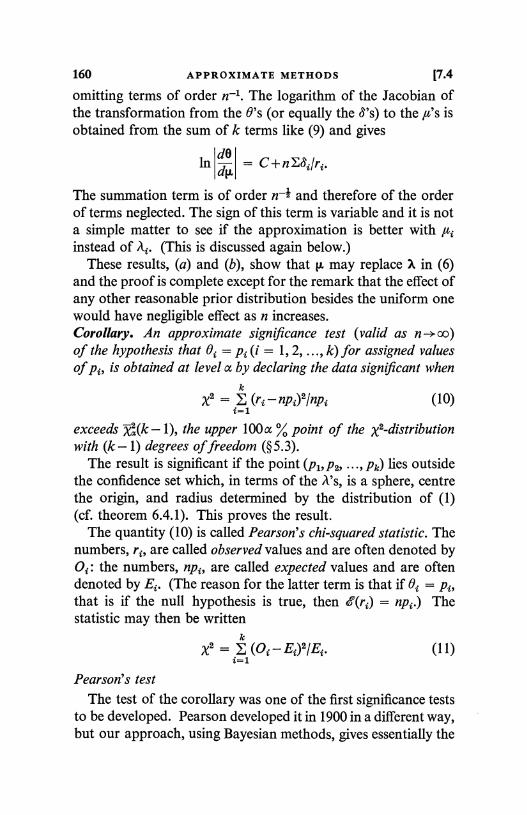
160 APPROXIMATE METHODS [7.4
omitting terms of order n-1. The logarithm of the Jacobian ofthe transformation from the B's (or equally the 8's) to the ,u's isobtained from the sum of k terms like (9) and gives
lnlde = C+nE8j/ri.
The summation term is of order n-1 and therefore of the orderof terms neglected. The sign of this term is variable and it is nota simple matter to see if the approximation is better with ,a2instead of A2. (This is discussed again below.)
These results, (a) and (b), show that 1L may replace a in (6)and the proof is complete except for the remark that the effect ofany other reasonable prior distribution besides the uniform onewould have negligible effect as n increases.Corollary. An approximate significance test (valid as n--*a )of the hypothesis that Oi = pi (i = 1, 2, ..., k) for assigned valuesof pi, is obtained at level a by declaring the data significant when
kx2 = (ri - npti)2/np (10)
i=1
exceeds x2(k-1), the upper 100a % point of the x2-distributionwith (k - 1) degrees of freedom (§5.3).
The result is significant if the point (Pi, P2, ..., pk) lies outsidethe confidence set which, in terms of the A's, is a sphere, centrethe origin, and radius determined by the distribution of (1)(cf. theorem 6.4.1). This proves the result.
The quantity (10) is called Pearson's chi-squared statistic. Thenumbers, ri, are called observed values and are often denoted byOi : the numbers, npi, are called expected values and are oftendenoted by Ei. (The reason for the latter term is that if 01 = pi,that is if the null hypothesis is true, then i7 (ri) = npi.) Thestatistic may then be written
kx2 = E (O1 -Ei)2/Ei. (11)
i=1
Pearson's testThe test of the corollary was one of the first significance tests
to be developed. Pearson developed it in 1900 in a different way,but our approach, using Bayesian methods, gives essentially the
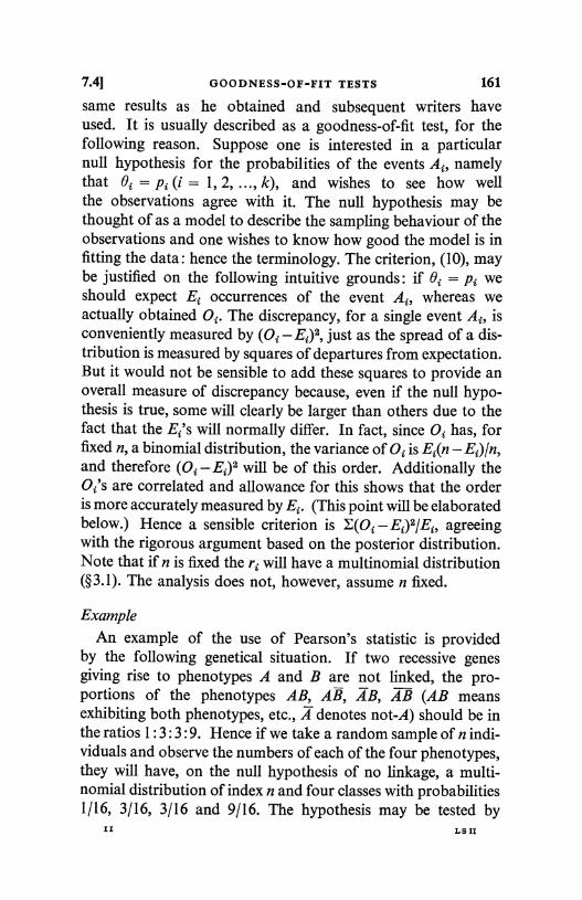
7.4] GOODNESS-OF-FIT TESTS 161
same results as he obtained and subsequent writers haveused. It is usually described as a goodness-of-fit test, for thefollowing reason. Suppose one is interested in a particularnull hypothesis for the probabilities of the events Ai, namelythat Oi = pi (i = 1, 2, ..., k), and wishes to see how wellthe observations agree with it. The null hypothesis may bethought of as a model to describe the sampling behaviour of theobservations and one wishes to know how good the model is infitting the data: hence the terminology. The criterion, (10), maybe justified on the following intuitive grounds: if 0i = pi weshould expect Ei occurrences of the event Ai, whereas weactually obtained Oi. The discrepancy, for a single event Ai, isconveniently measured by (Oi - Ei)2, just as the spread of a dis-tribution is measured by squares of departures from expectation.But it would not be sensible to add these squares to provide anoverall measure of discrepancy because, even if the null hypo-thesis is true, some will clearly be larger than others due to thefact that the Ei's will normally differ. In fact, since Oi has, forfixed n, a binomial distribution, the variance of Oi is Ei(n - Ei)ln,and therefore (Oi - Ei)2 will be of this order. Additionally theOi's are correlated and allowance for this shows that the orderis more accurately measured by Ei. (This point will be elaboratedbelow.) Hence a sensible criterion is E(Oi - Ei)2lEi, agreeingwith the rigorous argument based on the posterior distribution.Note that if n is fixed the ri will have a multinomial distribution(§3.1). The analysis does not, however, assume n fixed.
Example
An example of the use of Pearson's statistic is providedby the following genetical situation. If two recessive genesgiving rise to phenotypes A and B are not linked, the pro-portions of the phenotypes AB, AB, AB, TB_ (AB meansexhibiting both phenotypes, etc., A denotes not-A) should be inthe ratios 1:3:3:9. Hence if we take a random sample of n indi-viduals and observe the numbers of each of the four phenotypes,they will have, on the null hypothesis of no linkage, a multi-nomial distribution of index n and four classes with probabilities1/16, 3/16, 3/16 and 9/16. The hypothesis may be tested by
II LS II
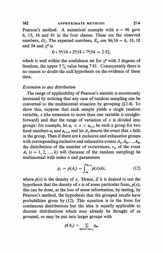
162 APPROXIMATE METHODS [7.4
Pearson's method. A numerical example with n = 96 gave6, 13, 16 and 61 in the four classes. These are the observednumbers, O. The expected numbers, Ei, are 96/16 = 6, 18, 18and 54 and x2 is
0+52/18+22/18+72/54 = 2.52,
which is well within the confidence set for x2 with 3 degrees offreedom, the upper 5 % value being 7.81. Consequently there isno reason to doubt the null hypothesis on the evidence of thesedata.
Extension to any distributionThe range of applicability of Pearson's statistic is enormously
increased by noticing that any case of random sampling can beconverted to the multinomial situation by grouping (§2.4). Toshow this, suppose that each sample yields a single randomvariable, x (the extension to more than one variable is straight-forward) and that the range of variation of x is divided intogroups : for example, let ai < x < ai+i be such a group for twofixed numbers ai and ai+1i and let Ai denote the event that x fallsin the group. Then if there are k exclusive and exhaustive groupswith corresponding exclusive and exhaustive events Al, A2,..., Ak,the distribution of the number of occurrences, ri, of the eventAi (i = 1, 2, ..., k) will (because of the random sampling) bemultinomial with index n and parameters
pi = p(Ai) = J
at+,p(x)dx,(12)
where p(x) is the density of x. Hence, if it is desired to test thehypothesis that the density of x is of some particular form, p(x),this can be done, at the loss of some information, by testing, byPearson's method, the hypothesis that the grouped results haveprobabilities given by (12). This equation is in the form forcontinuous distributions but the idea is equally applicable todiscrete distributions which may already be thought of asgrouped, or may be put into larger groups with
p(A1) = E 78,aids<ai+.
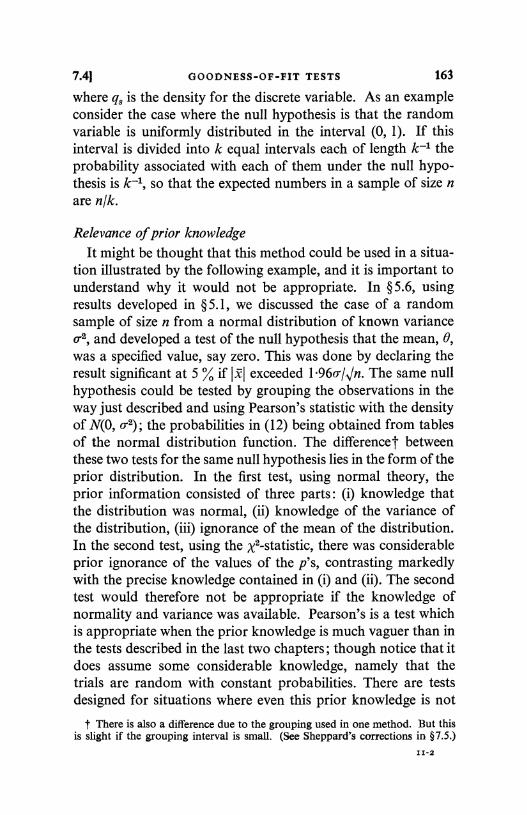
7.4) GOODNESS-OF-FIT TESTS 163
where qs is the density for the discrete variable. As an exampleconsider the case where the null hypothesis is that the randomvariable is uniformly distributed in the interval (0, 1). If thisinterval is divided into k equal intervals each of length k-1 theprobability associated with each of them under the null hypo-thesis is k-1, so that the expected numbers in a sample of size nare n/k.
Relevance of prior knowledgeIt might be thought that this method could be used in a situa-
tion illustrated by the following example, and it is important tounderstand why it would not be appropriate. In § 5.6, usingresults developed in § 5.1, we discussed the case of a randomsample of size n from a normal distribution of known variance0, and developed a test of the null hypothesis that the mean, 0,was a specified value, say zero. This was done by declaring theresult significant at 5 % if 1x1 exceeded 1.96o'/ /n. The same nullhypothesis could be tested by grouping the observations in theway just described and using Pearson's statistic with the densityof N(0, 0.2); the probabilities in (12) being obtained from tablesof the normal distribution function. The difference' betweenthese two tests for the same null hypothesis lies in the form of theprior distribution. In the first test, using normal theory, theprior information consisted of three parts : (i) knowledge thatthe distribution was normal, (ii) knowledge of the variance ofthe distribution, (iii) ignorance of the mean of the distribution.In the second test, using the X2-statistic, there was considerableprior ignorance of the values of the p's, contrasting markedlywith the precise knowledge contained in (i) and (ii). The secondtest would therefore not be appropriate if the knowledge ofnormality and variance was available. Pearson's is a test whichis appropriate when the prior knowledge is much vaguer than inthe tests described in the last two chapters; though notice that itdoes assume some considerable knowledge, namely that thetrials are random with constant probabilities. There are testsdesigned for situations where even this prior knowledge is not
t There is also a difference due to the grouping used in one method. But thisis slight if the grouping interval is small. (See Sheppard's corrections in §7.5.)
11-2
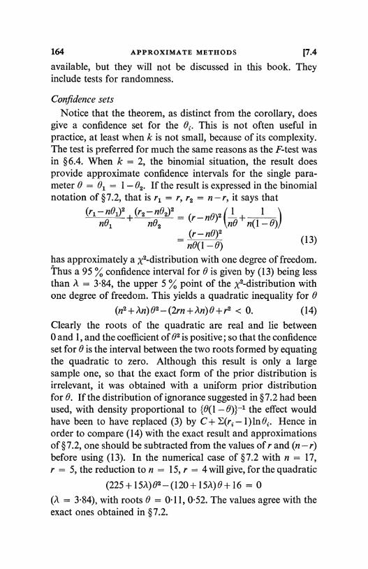
164 APPROXIMATE METHODS [7.4
available, but they will not be discussed in this book. Theyinclude tests for randomness.
Confidence sets
Notice that the theorem, as distinct from the corollary, doesgive a confidence set for the O. This is not often useful inpractice, at least when k is not small, because of its complexity.The test is preferred for much the same reasons as the F-test wasin § 6.4. When k = 2, the binomial situation, the result doesprovide approximate confidence intervals for the single para-meter 0 = 01 = 1- 02. If the result is expressed in the binomialnotation of § 7.2, that is r1 = r, r2 = n - r, it says that
(r1 - n01)2 (r2 - n02)2 2 1 1
nO1 + n02 = (r - n0) (n0 +n(1- 0))(r - n0)2
(13)n0(l -0)has approximately a x2-distribution with one degree of freedom.Thus a 95 % confidence interval for 0 is given by (13) being lessthan A = 3.84, the upper 5 % point of the X2-distribution withone degree of freedom. This yields a quadratic inequality for 0
(n2 + An) 02 - (2rn + An) 0 +r2 < 0. (14)
Clearly the roots of the quadratic are real and lie between0 and 1, and the coefficient of 02 is positive; so that the confidenceset for 0 is the interval between the two roots formed by equatingthe quadratic to zero. Although this result is only a largesample one, so that the exact form of the prior distribution isirrelevant, it was obtained with a uniform prior distributionfor 0. If the distribution of ignorance suggested in § 7.2 had beenused, with density proportional to {0(1- 0)}-1 the effect wouldhave been to have replaced (3) by C + E(r1-1) In 0i. Hence inorder to compare (14) with the exact result and approximationsof § 7.2, one should be subtracted from the values of r and (n - r)before using (13). In the numerical case of §7.2 with n = 17,r = 5, the reduction to n = 15, r = 4 will give, for the quadratic
(225+151)02-(120+151)0+16 = 0(A = 3.84), with roots 0 = 0- 11, 0.52. The values agree with theexact ones obtained in § 7.2.
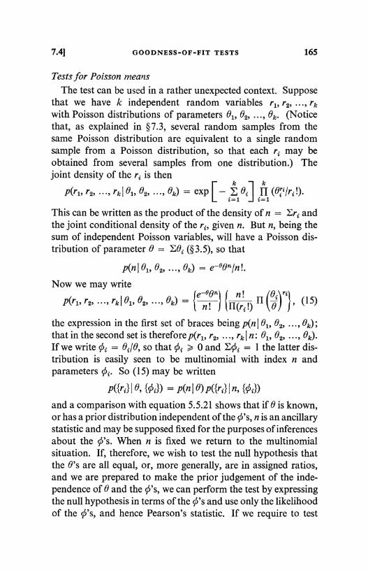
7.4] GOODNESS-OF-FIT TESTS 165
Tests for Poisson means
The test can be used in a rather unexpected context. Supposethat we have k independent random variables r1, r2, ..., rkwith Poisson distributions of parameters 01, 02, ..., 0k. (Noticethat, as explained in § 7.3, several random samples from thesame Poisson distribution are equivalent to a single randomsample from a Poisson distribution, so that each ri may beobtained from several samples from one distribution.) Thejoint density of the ri is then
k`7k-P(r1, r2, ..., rk 1611, 02, ..., 0k) = exp - u Bi H (O /ri !).
i=1 1 i=1
This can be written as the product of the density of n = Eri andthe joint conditional density of the r1, given n. But n, being thesum of independent Poisson variables, will have a Poisson dis-tribution of parameter 0 = E0i (§3.5), so that
P(nI 01, 02, ..., 0k) = e-Bon/n!.
Now we may write0i r
P(r1, r2, ..., rk 01, 02, ..., 0k)e-001 n!
= {-]---} 11(rz.!) Il (e) (15)
the expression in the first set of braces being p(n 01i 02, ..., 0k);that in the second set is therefore p(r1i r2, ..., rkI n : 01, 02, ..., 00-If we write ci = 0i/0, so that Oi > 0 and E0i = 1 the latter dis-tribution is easily seen to be multinomial with index n andparameters 0i. So (15) may be written
p({ri} 0, {Oi}) = p(n 0) p({ri} I n, {ci})
and a comparison with equation 5.5.21 shows that if 0 is known,or has a prior distribution independent of the ¢'s, n is an ancillarystatistic and may be supposed fixed for the purposes of inferencesabout the O's. When n is fixed we return to the multinomialsituation. If, therefore, we wish to test the null hypothesis thatthe 0's are all equal, or, more generally, are in assigned ratios,and we are prepared to make the prior judgement of the inde-pendence of 0 and the O's, we can perform the test by expressingthe null hypothesis in terms of the ¢'s and use only the likelihoodof the q's, and hence Pearson's statistic. If we require to test
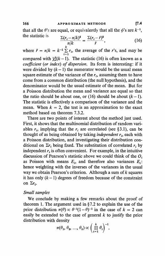
166 APPROXIMATE METHODS [7.4
that all the B's are equal, or equivalently that all the O's are k-1,the statistic is E(ri - n/k)2 E(ri - r)2
n/k r (16)
kwhere F = n/k = k-1 ri, the average of the r's, and may be
i=1compared with xa(k - 1). The statistic (16) is often known as acoefficient (or index) of dispersion. Its form is interesting: if itwere divided by (k-1) the numerator would be the usual meansquare estimate of the variance of the ri, assuming them to havecome from a common distribution (the null hypothesis), and thedenominator would be the usual estimate of the mean. But fora Poisson distribution the mean and variance are equal so thatthe ratio should be about one, or (16) should be about (k - 1).The statistic is effectively a comparison of the variance and themean. When k = 2, the test is an approximation to the exactmethod based on theorem 7.3.2.
There are two points of interest about the method just used.First, it shows that the multinomial distribution of random vari-ables ri, implying that the ri are correlated (see §3.1), can bethought of as being obtained by taking independent ri, each witha Poisson distribution, and investigating their distribution con-ditional on Eri being fixed. The substitution of correlated ri byindependent ri is often convenient. For example, in the intuitivediscussion of Pearson's statistic above we could think of the Oias Poisson with means Ei, and therefore also variances Ei:hence weighting with the inverses of the variances in the usualway we obtain Pearson's criterion. Although a sum of k squaresit has only (k - 1) degrees of freedom because of the constrainton Eri.
Small samplesWe conclude by making a few remarks about the proof of
theorem 1. The argument used in § 7.2 to explain the use of theprior distribution 1T(6) oc 0-1(1 - 6)-1 in the case of k = 2 caneasily be extended to the case of general k to justify the priordistribution with density
k -1
))i (e1, 02, ..., Ok) oc Oi1
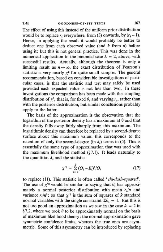
7.41 GOODNESS-OF-FIT TESTS 167
The effect of using this instead of the uniform prior distributionwould be to replace ri everywhere, from (3) onwards, by (ri - 1).Hence, in applying the result it would probably be better todeduct one from each observed value (and k from n) beforeusing it: but this is not general practice. This was done in thenumerical application to the binomial case k = 2, above, withsuccessful results. Actually, although the theorem is only alimiting result as n oo, the exact distribution of Pearson'sstatistic is very nearly x2 for quite small samples. The generalrecommendation, based on considerable investigations of parti-cular cases, is that the statistic and test may safely be usedprovided each expected value is not less than two. In theseinvestigations the comparison has been made with the samplingdistribution of x2, that is, for fixed Oi and varying ri, rather thanwith the posterior distribution, but similar conclusions probablyapply to the latter.
The basis of the approximation is the observation that thelogarithm of the posterior density has a maximum at 9 and thatthe density falls away fairly sharply from this maximum. Thelogarithmic density can therefore be replaced by a second-degreesurface about this maximum value: this corresponds to theretention of only the second-degree (in Si) terms in (5). This isessentially the same type of approximation that was used withthe maximum likelihood method (§7.1). It leads naturally tothe quantities xi, and the statistic
kx'2 = Z (0i - Ei)2/Oi
i=1(17)
to replace (11). This statistic is often called 'chi-dash-squared'.The use of x'2 would be similar to saying that ei has approxi-mately a normal posterior distribution with mean ri/n andvariance ri/n2; so that x'2 is the sum of squares of k standardnormal variables with the single constraint EBi = 1. But this isnot too good an approximation as we saw in the case k = 2 in§ 7.2, where we took 0 to be approximately normal on the basisof maximum likelihood theory: the normal approximation gavesymmetric confidence limits, whereas the true ones are asym-metric. Some of this asymmetry can be introduced by replacing
168 APPROXIMATE METHODS [7.4
Oi in the denominator of (17) by E1, and we saw above, in onenumerical example, that this introduces the required degree ofasymmetry. In general, the improvement in the approximationobtained by using Ei is reflected in the smaller size of the highest-order term neglected in the expansion of the logarithm of theposterior density. The term of order n_I in (8) is only half themagnitude of the corresponding term in (5), and the Jacobianof the transformation introduces a term of order n-t, equation(9), which, on the average is zero, since e(88 I 0i) = 0.
One great limitation of Pearson's statistic as developed in thissection is that it is only available for testing a completely speci-fied hypothesis, namely that all the 0i's are equal to assignedvalues pi. There are many situations where one wishes to test ahypothesis which only partially specifies the 0i's. For example,we have described how to test the hypothesis that a randomsample comes from a normal distribution of specified mean andvariance, but we cannot, using the methods of this section, testthe less specific hypothesis that it comes from some normaldistribution. It is to the type of problems of which this is anexample that we turn in the next section.
7.5. Goodness-of-fit tests (continued)
The notation is the same as that of the previous section.
Theorem 1. If, in each of a random sequence of n trials, theexclusive and exhaustive events Ai (i = 1, 2, ..., k) have constantprobabilities of success 01 and occur ri times (Eri = n); then anapproximate significance test (valid as n =- oo) of the hypothesisthat 1 ( < k) functions, functionally independent of each other andof Z0j, are all zero,
X1(01, 02, ..., Bk) = c21e1, 02, ..., 0k) c1(01, 02, ..., 0k)
= 0, (1)
is obtained at level a by declaring the data significant when
k
x2 = (ri - n#i)2/nOi (2)i=1
exceeds )&(l), the upper 100x% point of the x2-distribution
7.51 GOODNESS-OF-FIT TESTS 169
with 1 degrees of freedom, where ti is the maximum likelihoodestimate of Oi assuming that (1) obtains.
We shall use the asymptotic result of theorem 7.4.1. Thatresult was based on the remark that the posterior distributionhad a maximum at Oi = ri/n and that 6i = 0i - rj/n would besmall, in fact of order n-I, so that only a small region in theneighbourhood of the maximum need be considered. In thatregion it will be assumed that the functions 0j of (1) are suffici-ently smooth for them to be replaced by linear functions of theO's: that is, we suppose that the constraints gi = 0 (1 = 1, 2, ..., l)can be approximately written
k
aij Oj = cij=1
for i = 1, 2, ..., 1. These may alternatively be written
ajj )j = cj,j=1
(3)
(4)
k
where aij = aijV(rj)/n and ci' = ci- aijrj/n, and, as in §7.4,j=1
Ai = n8j/Jrj = n(0j - r1/n)/Vr1. (5)
Now it is well known (see, for example, most books onlinear algebra) that an orthogonal k x k matrix with elementsbij can be found such that the restrictions imposed on the A's by(4) are equivalent to the restrictions
k
E bij Aj = di, (6)j=1
for i = 1, 2, ..., 1. (For this to be so it is necessary that the O's,and hence the left-hand sides of (3), be independent functions ofthe 0's.) Define new parameters 3/r j by the equations
k
Vi = jE bijA1, (7)
for all i, so that the constraints (6) are ;/rj = dj for i 5 1. Thenthe hypothesis we are interested in testing is that 3rj = di fori < 1, and the parameters Vri for i > 1 are not of interest to us.In accord with the general principles of inference we have to
170 APPROXIMATE METHODS [7.5
find the posterior distribution of the zfr's involved in the hypo-thesis; that is, i for i < 1.
Now from equation 7.4.61k
lnir(AIr) = C-2Ax2 (8)
to the order of approximation being used. It immediatelyfollows that to the same order
kC-2 tj (9)
since the Jacobian is unity. This result follows because thematrix of elements bi; is orthogonal. Consequently, integratingthe posterior probability density with respect to +fri+1, W 1+2, k
In rr(3r1, Y' 2, ..., rl I r) = C - 2 ZE fri. (10)
Also since the O's are independent of 10i, so are the ifri's fori < l and hence there is no linear relation between the Vri'sin (10). It follows as in theorem 6.4.2 that the distribution of
a
2 is x2 with 1 degrees of freedom and hence that a significancei=1
a
test is obtained by declaring the data significant if E 0t exceedsi=1
da(l). It remains to calculate di.i=1
Since, in deriving (8), and hence (9), the prior distribution ofthe 0's was supposed uniform, the right-hand side of (9) is equallythe logarithm of the likelihood of the zfr's, the lfr's being linearfunctions of the 0's. If (1) obtains this logarithmic likelihood is
I a I kC-- Ed2- E2i=1 2i+1with maximum obtained by putting Y' i = 0 for i > 1, giving
I
C-21iEdi.k
Consequently 22E d4 is equal to the value of 22E Al at the
maximum likelihood values of the 0's when (1) obtains. This
7.51 GOODNESS-OF-FIT TESTS 171
proves the result with ri instead of nOi in the denominator of (2).We may argue, as in the proof of theorem 7.4.1, that the replace-ment will not affect the result as n -* oo. The theorem is thereforeproved.
The quantity (2) may be written in Pearson's form
E(Oi - Ei)2/Ei, (11)
provided the Ei are suitably interpreted. Ei is the expectednumber of occurrences of Ai if the maximum likelihood valueunder the null hypothesis were the true value.
Special case: 1 = k-1The corollary to theorem 7.4.1 is a special case of the above.
In that corollary the null hypothesis being tested was completelyspecified so that the number of functions in (1) must be 1= k - 1,which, together with Eoi = 1, completely determine the 0's.Since the 0's are completely determined at values pi it followsthat of = pi and (2) reduces to (7.4.10), the degrees of freedombeing l = k -1.
Test for a binomial distributionIn the last section we saw how to test the hypothesis that a
random sample comes from a completely specified distribution;for example, binomial with index' s and parameter p, wheres and p are given. The new result enables a test to be made of thehypothesis that a random sample comes from a family of distri-butions; for example, binomial with index s, the parameterbeing unspecified. To do this suppose that we have n observa-tions, all integer and between 0 and s, of independent randomvariables from a fixed, but unknown distribution which may bea binomial distribution with index s. Let the number ofobservations equal to i be ri (0 < i < s), so that Erj = n. Thenthe is have a multinomial distribution, with index s + 1 (sincethe original random variables are supposed independent andfrom a fixed distribution) and if the further assumption is made
t We use s, instead of the usual n, for the index in order not to confuse it withthe value n of the theorem.
172 APPROXIMATE METHODS [7.5
that the distribution is binomial, the parameters of the multi-nomial distribution will be, for 0 < i S s,
Oi = (il 0i(1- 0)3-i, (12)
where 0 is the unknown binomial parameter. If 0 were specified,say equal top, the Oi would be known by putting 0 = p in (12);the Ei would be nOi and Pearson's statistic could be used withs degrees of freedom. But if 0 is unknown it has to be estimatedby maximum likelihood. The logarithm of the likelihood is,apart from a constant, Eri In 0i (equation 7.4.3) or, by (12),
s s
iriln0+ (s-i)riln(1-0). (13)i=0 i=0
The maximum is easily seen (cf. §7.1) to be given by3
0 _ E iri/ns. (14)i=0
Consequently if 0, in (12), is put equal to 0 the resulting values Oimay be used to compute expected values nOi and Pearson'sstatistic compared with ;V2.
Degrees of freedomIt only remains to determine the degrees of freedom. Accord-
ing to the theorem the number of degrees of freedom is equal tothe number of constraints on the 0i that the null hypothesis (12)imposes. The latter number is most easily determined byremarking that the number of 0i's (the number of groups) iss + 1, the k of the theorem, and hence the values of s (= k - 1)constraints (apart from EOi = 1) are needed to specify the0i's completely : but the binomial hypothesis leaves only onevalue, 0, unspecified so that it must implicitly specify (s-1)constraints. Hence there are (s-1) constraints in (1): that isl = s - 1 and the degrees of freedom are therefore s - 1.
This method of obtaining the degrees of freedom is alwaysavailable and is often useful. In essence, one considers thenumber of constraints, additional to those in (1), that wouldhave to be specified in order to determine all the 0i's. If thisnumber is m, then I+ m = k - 1 and the degrees of freedom are
7.5] GOODNESS-OF-FIT TESTS 173
1 = (k -1) - m. There is a loss of one degree of freedom foreach unspecified constraint in the null hypothesis. Each suchconstraint corresponds to a single unspecified parameter in thenull hypothesis (here 0) and the rule is that there is a loss of onedegree of freedom for each parameter that has to be estimatedby maximum likelihood. Rather roughly, the ability to varyeach of these parameters enables one to make the Ei agree moreclosely with the Oi, so that the statistic is reduced, and this isreflected in a loss of degrees of freedom-the mean value of x2being equal to the degrees of freedom (§5.3). The result on thereduction in the degrees of freedom is due to Fisher; Pearsonhaving been under the mistaken impression that no correctionfor estimation was necessary.
Test for Poisson distribution
Similar ideas may be applied to any discrete distribution.Another example would be the Poisson distribution; but therethe number of possible values would be infinite, namely all non-negative integers, and some grouping would be necessary, asexplained in § 7.4. Usually it will be enough to group all obser-vations not less than some value c, and suppose them all equalto c, the value of c being chosen so that the expectation is notbelow about two. This introduces a slight error into the maxi-mum likelihood estimation, but this is not likely to be serious.It is important to notice the difference between this type oftest and the test for Poisson distributions in §7.4. The latterwas for the differences between Poisson means; that is, the dis-tributions were assumed, because of prior knowledge, to bePoisson and only their means were compared. The present testsupposes it known only that the variables come from somedistribution and asks if that distribution could be Poisson.There is obviously less prior knowledge available here andconsequently a larger sample is needed to produce a useful test.
Continuous distributions
The same ideas may be applied to fitting a continuous distri-bution : for example, we might ask if the variables come froman unspecified normal distribution. The observations would be
174 APPROXIMATE METHODS [7.5
divided into k convenient groups and the numbers ri in thedifferent groups counted. It only remains to find the maximumlikelihood estimates of the 8i when the null hypothesis is true.If the null hypothesis distribution depends on parametersal, a2, ..., a8 and has densityp(xI a1, a2, ..., a8), the Bi's are givenby (cf. equation 7.4.12)
0i = P(xIa,, a2, ..., a.) dx, (15)ai
and the logarithm of the likelihood is as usual. The maximumlikelihood estimation presents some difficulties because theequations to be solved are
kriOi 1aOi/aa; = 0 (j = 1, 2, ..., s) (16)
i=1
and the partial derivatives can be awkward. It is usual toapproximate to (15) by assuming the density approximatelyconstant in the interval when, if gi is some point in the interval,
6i = P(gi I all a2, ..., a8) (ai+1- ai) (17)
The maximum likelihood equations are thenk
E ri alnP(6i I ai, a2, ..., a8)/aaf = 0 (j = 1, 2, ..., s). (18)i=1
If each observation x, (t = 1, 2, ..., n) is replaced by the value6i of the group to which it belongs (there then being ri x's whichyield a value Fi), equations (18) are the ordinary maximum likeli-hood equations for the a's when the sample values are the f'sand the density is p(x I all a2, ..., a8). These may be easier tosolve than (16). Thus with the normal case where there are twoparameters, the mean and the variance, this gives the usualestimates (equation 7.1.12-where the present a's are there 0's)in terms of the grouped values, F.. These estimates can then beinserted in (17), or (15), to obtain the 6i. The procedure may besummarized as follows : (i) replace the observed values x, by thegrouped values 6i; (ii) estimate the parameters in the density bymaximum likelihood applied to the Si, (18); (iii) estimate the Bifrom (15) or (17); (iv) use these estimates in the x2 statistic (2),
7.5] GOODNESS-OF-FIT TESTS 175
subtracting a degree of freedom for each parameter estimated.Thus with the normal distribution the degrees of freedom willbe (k-l)-2 = k-3.
Sheppard's correctionsThe replacement of (16) by (18) can lead to systematic errors.
They can be reduced by a device which we illustrate for the casewhere there is a single unspecified parameter in the family ofdistributions, which will be denoted in the usual way by 0, andwhere the grouping intervals are equal (except for the end oneswhich will have to be semi-infinite). Equation (15) may bewritten Z+j n
0Z = f p(x10)dx (19)
for a convenient origin. An expansion in Taylor series gives animprovement on (17), namely
Bi = hp + 24P",
where the arguments of p are ih (formerly 5i) and 0, a remainderterm has been ignored, and dashes denote differentiation withrespect to x. Consequently
1nOi = lnhp+In 1+242
p] = lnhp+24 pto the same order, and
0 180i/a080
In p + 24 8 P I . (20)
We have to solve (16) with al = 0. This is easily seen to beequivalent to summing the right-hand side of (20) over theobservations at their grouped values and equating to zero. (Theequation is the same as (18) with the addition of the term in h2.)This equation can be solved by Newton's method (§7.1) witha first approximation given by 0(1), the root of (18). The secondapproximation is seen, from (7.1.17), to be 0(2) = 0a>+0, where
_h2
n
a 2(1nP)} . (21)24 t_180 p t1 a0
Here the xi have been replaced by their grouped values and the
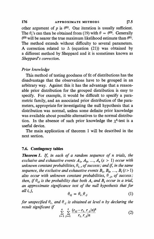
176 APPROXIMATE METHODS [7.5
other argument of p is B(l). One iteration is usually sufficient.The Bi's can then be obtained from (19) with 0 = 0(2). Generally0(2) will be nearer the true maximum likelihood estimate than Ba>.The method extends without difficulty to several parameters.A correction related to A (equation (21)) was obtained bya different method by Sheppard and it is sometimes known asSheppard's correction.
Prior knowledgeThis method of testing goodness of fit of distributions has the
disadvantage that the observations have to be grouped in anarbitrary way. Against this it has the advantage that a reason-able prior distribution for the grouped distribution is easy tospecify. For example, it would be difficult to specify a para-metric family, and an associated prior distribution of the para-meters, appropriate for investigating the null hypothesis that adistribution was normal, unless some definite prior knowledgewas available about possible alternatives to the normal distribu-tion. In the absence of such prior knowledge the X2-test is auseful device.
The main application of theorem 1 will be described in thenext section.
7.6. Contingency tables
Theorem 1. If, in each of a random sequence of n trials, theexclusive and exhaustive events Al, A2, ..., A3 (s > 1) occur withunknown constant probabilities, Bi., of success; and if, in the samesequence, the exclusive and exhaustive events B1, B2, ..., Bt (t > 1)also occur with unknown constant probabilities, 6.1, of success;then, if Bit is the probability that both Ai and B; occur in a trial,an approximate significance test of the null hypothesis that forall i, j,
oil = 01.0.1 (1)
for unspecified Bi. and 6.t is obtained at level a by declaring theresult significant if
E(r11- r1 r. 1/n)2
(2)i=1 j-1 ri. r.>ln

7.6] CONTINGENCY TABLES 177
exceeds X2 (V), where v = (s - 1) (t - 1). In (2), r15 is the numberof times that both Ai and B; occur in the n trials, so that E rj = n,andt t a
ri. = E r15, rij,j=1 i=1
i,i
(3)
so that these are respectively the number of times that A1, and thenumber of times that By, occur in the n trials.
The situation here described is essentially the same as that oftheorem 7.5.1 with a random sequence of n trials and k = stexclusive and exhaustive events, namely the simultaneous occur-rence of Ai and B;, the events Ai B; in the notation of § 1.2. Thenull hypothesis (1) puts some constraints on the probabilities ofthese events and says that the events Ai and Bf are independent,that is
p(Ai B,) = p(Ai)p(Bj),
without specifying the individual probabilities of the A's and B's.Theorem 7.5.1 can therefore be applied. We have only to deter-mine (a) the maximum likelihood estimates of Oil under the nullhypothesis, (1), and (b) the number, 1, of constraints involvedin (1).
(a) The logarithm of the likelihood is, if (1) obtains,
C+E ri5ln(0i.0.5) = C+E ri,ln0i,+E r,fln05.
Remembering that E 01. = E 0., = 1 we see easily (comparei i
the proof of theorem 7.4.1) that the maximum likelihood esti-mates of ei, and O. j are respectively ri.In and r,t/n. Hence
nOit = ri.r.3/n. (4)
(b) As in the applications in the last section it is easiest tocalculate 1 by finding the number of parameters unspecified inthe null hypothesis. Here it is obviously the number of func-tionally independent 01. and 04, that is, (s - 1) + (t - 1). Hence
1 = (st-1)-(s-1)-(t-1) = st-s-t+1 = (s-1)(t-1) = P.
t Notice that the dot suffix is here used slightly differently from previously(§ 6.4). Thus ri. denotes the sum over the suffix j, not the mean.
12 LSII
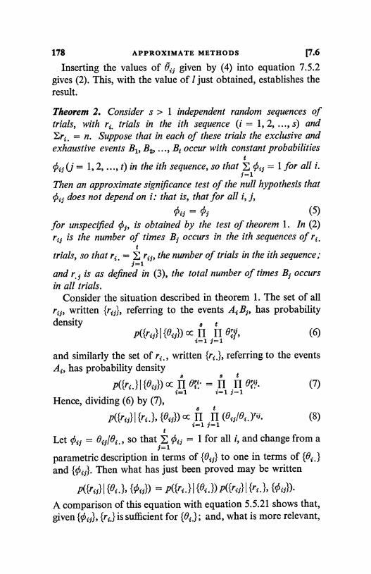
178 APPROXIMATE METHODS [7.6
Inserting the values of Oij given by (4) into equation 7.5.2gives (2). This, with the value of I just obtained, establishes theresult.
Theorem 2. Consider s > 1 independent random sequences oftrials, with rz_ trials in the ith sequence (i = 1, 2, ..., s) andEri. = n. Suppose that in each of these trials the exclusive andexhaustive events B1, B2, ..., Bt occur with constant probabilities
tOij (j = 1, 2, ..., t) in the ith sequence, so that E oij = 1 for all i.
J=1
Then an approximate significance test of the null hypothesis thateij does not depend on is that is, that for all i, j,
011 = 0j (5)for unspecified O, is obtained by the test of theorem 1. In (2)rij is the number of times Bj occurs in the ith sequences of ri.
t
trials, so that r1 _ ri3, the number of trials in the ith sequence;j=1
and r.j is as defined in (3), the total number of times Bj occursin all trials.
Consider the situation described in theorem 1. The set of allrij, written {rij}, referring to the events Ai Bj, has probabilitydensity 8 t
P({rij}I {eij}) oc II II e31; (6)i=1 j=1
and similarly the set of ri., written {ri.}, referring to the eventsAi, has probability density
8 8 t
P({ri. } I {eij}) cc n e%i' = II II e,rtij.i=1 i=1 j=1
Hence, dividing (6) by (7),8 t
P({rij}I {ri.}, {eij}) °C H H (eijlei.)riJ-i=1 y=1
(7)
(8)
t
Let Oi j =eij/ei., so that Z ¢ij = 1 for all i, and change from aj=1
parametric description in terms of {eij} to one in terms of {ei,}and {Oi j}. Then what has just been proved may be written
P({rij} I A.), {0o)) = P({ri. } I {ei.}) P({rij} I {ri. }, {0ij}).
A comparison of this equation with equation 5.5.21 shows that,given {0ij}, {r J is sufficient for {0J; and, what is more relevant,
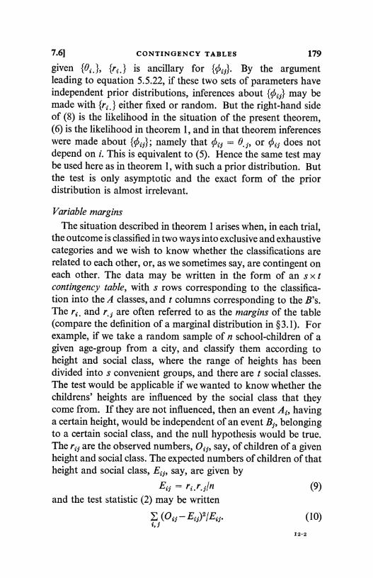
7.6] CONTINGENCY TABLES 179
given {0i.}, {ri,} is ancillary for {0ii}. By the argumentleading to equation 5.5.22, if these two sets of parameters haveindependent prior distributions, inferences about {0i;} may bemade with {ri _ } either fixed or random. But the right-hand sideof (8) is the likelihood in the situation of the present theorem,(6) is the likelihood in theorem 1, and in that theorem inferenceswere made about {Oii}; namely that ¢it = 0.j, or Oij does notdepend on i. This is equivalent to (5). Hence the same test maybe used here as in theorem 1, with such a prior distribution. Butthe test is only asymptotic and the exact form of the priordistribution is almost irrelevant.
Variable margins
The situation described in theorem 1 arises when, in each trial,the outcome is classified in two ways into exclusive and exhaustivecategories and we wish to know whether the classifications arerelated to each other, or, as we sometimes say, are contingent oneach other. The data may be written in the form of an s x tcontingency table, with s rows corresponding to the classifica-tion into the A classes, and t columns corresponding to the B's.The ri. and r,, are often referred to as the margins of the table(compare the definition of a marginal distribution in §3.1). Forexample, if we take a random sample of n school-children of agiven age-group from a city, and classify them according toheight and social class, where the range of heights has beendivided into s convenient groups, and there are t social classes.The test would be applicable if we wanted to know whether thechildrens' heights are influenced by the social class that theycome from. If they are not influenced, then an event Ai, havinga certain height, would be independent of an event B,, belongingto a certain social class, and the null hypothesis would be true.The ri1 are the observed numbers, Oi;, say, of children of a givenheight and social class. The expected numbers of children of thatheight and social class, Eif, say, are given by
Ei, = ri.r.;lnand the test statistic (2) may be written
(9)
E(Oij - E,)2/Ej. (10)
12-2
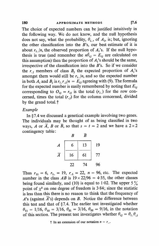
180 APPROXIMATE METHODS [7.6
The choice of expected numbers can be justified intuitively inthe following way. We do not know, and the null hypothesisdoes not say, what the probability, Oi., of Ai, is; but, ignoringthe other classification into the B's, our best estimate of it isabout ri. In, the observed proportion of Ai's. If the null hypo-thesis is true (and remember the nOi; = E'if are calculated onthis assumption) then the proportion of Ai's should be the same,irrespective of the classification into the B's. So if we considerthe r,; members of class B; the expected proportion of Ai'samongst them would still be r. In, and so the expected numberin both Ai and B; is Ei; agreeing with (9). The formulafor the expected number is easily remembered by noting that Ei;corresponding to Oi; = ri; is the total (ri.) for the row con-cerned, times the total (r.) for the column concerned, dividedby the grand total. j'
ExampleIn § 7.4 we discussed a genetical example involving two genes.
The individuals may be thought of as being classified in twoways, A or A,BorB,sothats= t = 2and wehavea2x2contingency table :
A
A
B B
6 13 19
16 61 77
22 74 96
Thus r11 = 6, r1 = 19, r,1 = 22, n = 96, etc. The expectednumber in the class AB is 19 x 22/96 = 4.35, the other classesbeing found similarly, and (10) is equal to 1.02. The upper 5 %point of x2 on one degree of freedom is 3.84; since the statisticis less than this there is no reason to think that the frequency ofA's (against A's) depends on B. Notice the difference betweenthis test and that of §7.4. The earlier test investigated whether01, = 1/16, 012 = 3/16, 021 = 3/16, 022 = 9/16, in the notationof this section. The present test investigates whether Oij = Oi.O, j
t In an extension of our notation n = r...
7.6] CONTINGENCY TABLES 181
for all i, j, and a little calculation shows that this is equivalentto 011/012 = 021/022. The question asked here is less specific thanthat of §7.4.
The computational problem of dealing with a contingencytable of general size may be reduced in the case of a 2 x 2 tableby noting that (2) may, in that special situation, be written
rll r22 - r12 r22rc
r1.r.1r2.r.2
This can be proved by elementary algebra.
One margin fixed
The situation considered in theorem 2 is rather different. Tochange the language a little : in the first theorem we have a singlesample of n individuals, each classified in two ways; in thesecond theorem we have s independent samples in which eachindividual is classified in only one way. However, the secondsituation may be related to the first by regarding the s samplesas another classification, namely classifying the individualaccording to the number of the sample to which he belongs.The first stage in the proof of theorem 2 is to show that in thefirst situation with n individuals, the conditional probabilitydistribution of the individuals with regard to the second (the B)classification given the first (the A) classification is the same asin the second situation, with the A-classification being into thedifferent samples. Or, more mathematically, the probabilitydistribution of the entries in the table (the r1) given one set ofmargins (r1) is the same as the distribution of s samples ofsizes ri.. Furthermore the distribution of the margin does notdepend on the parameters of interest. The situation therefore isexactly that described in equation 5.5.21 with 02 there being thepresent ¢'s. Consequently inferences about the O's may be madein the same way whether the margins are fixed or random. Ifthey are random theorem 1 shows us how to make the signifi-cance test. Therefore the same test can be used in the situationof theorem 2 with the margin fixed. There is another way oflooking at the same situation. As an example of an ancillarystatistic in § 5.5 we took the case of a random sample of size n,
182 APPROXIMATE METHODS [7.6
where n may have been chosen randomly according to a distri-bution which did not depend on the parameter of interest. Wesaw that n was ancillary and could therefore be supposed fixed.Here we have s samples of different sizes, possibly random,rl., r2,, ..., rs.; these sizes having a distribution which does notdepend on the parameters, ¢i;, of interest. Exactly as beforethey may be supposed fixed.
The null hypothesis tested in theorem 2 is that the probabilitiesof the events Bt are the same for all samples: that is, the classifi-cation by the B's is not contingent on the sample (or equiva-lently the classification by the A's). It would arise, for example,if one took random samples of school-children of a given age-group in a city from each of the social classes, and asked if thedistribution of height varied with the social class. The computa-tions would be exactly the same as in the former example wherethe numbers in the social classes were also random.
Binomial distributionsThe situation of theorem 2 with s = t = 2 is the same as
that considered in §7.2 for the comparison of the probabilitiesof success in two random sequences of trials. The x2-testprovides a much more widely used alternative to that usingequation 7.2.17 based on the logarithmic transformation of theodds. The earlier test has the advantage that it can be extendedto give confidence intervals for the ratio of odds in the twosequences. It is not common practice to quote confidencelimits in dealing with contingency tables for much the samereasons as were discussed in § 6.5 in connexion with the analysisof variance. But, where possible, this should certainly be done;or better still, the posterior distribution of the relevant para-meter, or parameters, quoted.
The situation of theorem 2 with t = 2 and general s is thecomparison of several probabilities of success in several randomsequences of trials. The distribution of the ril will be B(ri., Oil)and the null-hypothesis is that Oil = 0 for all i, with ¢ unspeci-fied. It is easily verified that if ri. = n, say, ' the same for all i,
t We use n because it is the index of the binomial distribution. The n of thetheorems is now sn.
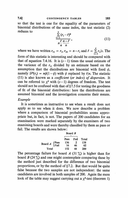
7.6] CONTINGENCY TABLES 183
so that the test is one for the equality of the parameters ofbinomial distributions of the same index, the test statistic (2)reduces to 8
(ri - r)2i=1
rn-rn-n n
8
where we have written ri1 = ri, ri2 = n - ri and F = E ri/s. Thei=1
form of this statistic is interesting and should be compared withthat of equation 7.4.16. It is (s - 1) times the usual estimate ofthe variance of the r1, divided by an estimate based on theassumption that the distributions are binomial with fixed 0,namely _9 2(r) = nc(l - 0) with 0 replaced by r/n. The statistic(11) is also known as a coefficient (or index) of dispersion. Itcan be referred to x2 with (s - 1) degrees of freedom. The testshould not be confused with that of §7.5 for testing the goodnessof fit of the binomial distribution: here the distributions areassumed binomial and the investigation concerns their means.
ExampleIt is sometimes as instructive to see when a result does not
apply as to see when it does. We now describe a problemwhere a comparison of binomial probabilities seems appro-priate but, in fact, is not. The papers of 200 candidates for anexamination were marked separately by the examiners of twoexamining boards and were thereby classified by them as pass orfail. The results are shown below:
Board B
Pass Fail Total
Board A Pass 136 2 138Fail 16 46 62
Total 152 48 200
The percentage failure for board A (31 %) is higher than forboard B (24 %) and one might contemplate comparing these bythe method just described for the difference of two binomialproportions, or by the method of § 7.2. But that would be quitefalse because the two samples are not independent: the samecandidates are involved in both samples of 200. Again the merelook of the table may suggest carrying out a x2-test (theorem 1)
184 APPROXIMATE METHODS [7.6
on a 2 x 2 contingency table, but this would ask whether theproportion passing with board B was the same for those whofailed with board A as for those who passed with board A,a question of no interest. What one wishes to know is whetherone board has a higher failure rate than the other-the questionthat would have been answered by the first test had it beenvalid. To perform a test we note that the 182 candidates whowere treated similarly by the two boards (both failed or bothpassed) can provide no information about the differencesbetween the boards : so our interest must centre on the 18 othercandidates. We can see this also by remarking that in the tableas arranged the likelihood is, assuming the candidates to bea random sample,
811 012 821 022
{(011 + 022)r11+rz2(012 + 021)r12+rzl}
0110222 0122 021 l1X j}011 +
022)rl,+r22 (012 + 02_lr1z+r21}
= LY 11+rzz(1 - b1)rriz+r21} 1211(1 -V 2)r22) {Y 218(1 - Y 3)r21}, (12)
where V fl = 011 + 022, V f2 = 011011 + 022) and f3 = 8121(012 + 021)We are only interested in 3/r3 which is the probability, given thatthe candidate has been treated differently by the two boards,that he has been failed by B and passed by A. By the principleof ancillary statistics we can therefore consider only r12 and r21,provided our prior judgment is that l1rl and / 2 are independentof t/r3, which is reasonable. From the last set of braces in (12),the likelihood is seen to be of the form appropriate to r12+r21independent trials with constant probability u 3 If the boardsare acting similarly 1/3 = # and it is this hypothesis that wemust test. The exact method is that of §7.2. From equation7.2.13 a confidence interval for 1/r3 is
(I+ 8F')-l < Vr3 < (I+ 8F 1)-1.
With 4 and 32 degrees of freedom and a = 0.05, P = 322 (using2a = 0.025) and F' = 8.45 so that 0.015 < 3/r3 < 0.29 withprobability 0.95. The value 2 is outside the interval and thereis evidence that board A is more severe than board B.
7.6] SUGGESTIONS FOR FURTHER READING 185
Suggestions for further reading
The suggestions given in chapter 5 are adequate.
Exercises1. An individual taken from a certain very large biological population isof type A with probability -21(l + F) and of type B with probability J(1- F).Give the probability that a random sample of n such individuals will consistof a of type A and b of type B. Find P, the maximum likelihood estimateof F. Show that the expectation of P is F. Calculate the informationabout F. (Camb. N.S.)
2. A random sample is drawn from a population with density function
f(xIO) = 10
_e a-6x (0 < x < 1).
Show that the mean of the sample is a sufficient statistic for the parameter0 and verify that the maximum likelihood estimate is a function of thesample mean. Let this estimate be denoted by 0,L.
Suppose that the only information available about each sample memberconcerns whether or not it is greater than a half. Derive the maximumlikelihood estimate in this case and compare its posterior variance withthat of 01. (Wales Dip.)
3. A continuous random variable x, defined in the range 0 < x < fir, hasdistribution function proportional to (1-e-°`g'IIx) where a > 0. Find thedensity function of x.
Given a random sample of n observations from this distribution, derivethe maximum.likelihood equation for &, the estimate of a. Indicate verybriefly how this equation can be solved numerically.
Also prove that the posterior variance of a is
4&2 sinh2 }&
sinh2jLj -&2) (Leic. Gen.)
4. Calculate the maximum likelihood estimate, 0, of 0, the parameter ofthe Cauchy distribution
dF =7T l + (x - 0)2
dx (- oo < x < on),
given the sample of 7 observations,
3.2, 2.0, 2.3, 10.4, 1.9, 0.4, 2.6.
Describe how you could have used this calculation to determine approxi-mate confidence limits for 0, if the sample had been a large one.
(Manch. Dip.)
5. Independent observations are made on a Poisson variable of unknownmean 0. It is known only that of n observations, no have the value 0,nl have the value 1, and the remaining n - no - nl observations have values
186 APPROXIMATE METHODS
greater than one. Obtain the equation satisfied by the maximum likelihoodestimate and suggest how the equation could be solved numerically.
(Lond. B.Sc.)
6. The random variables X1, ..., Xm, Xm+l, ..., Xm+, are independently,normally distributed with unknown mean 0 and unit variance. AfterXl, ..., X. have been observed, it is decided to record only the signs ofXm+1, ..., X,,. Obtain the equation satisfied by the maximum likelihoodestimate 0, and calculate an expression for the asymptotic posteriorvariance of 0. (Lond. M.Sc.)
7. In an experiment on the time taken by mice to respond to a drug, thelog dose xi received by mouse i is controlled exactly, and the log responsetime tt is measured individually for all mice responding before log time T.The results of the experiment consist of (n-r) pairs (x;, t;) with t; 5 T,and r pairs in which xi is known exactly, but t, is `censored', and is knownonly to be greater than T. It is known that tj is normally distributed withknown uniform variance O'2, about the regression line
,'-V,) = a+,#x;,
where a and /3 are unknown. Verify that the following iterative procedurewill converge to the maximum likelihood estimates of a and /3.
(i) Using preliminary estimates a1 and b1, calculate y for each `censored'observation from the formula
T-al-blxjlyc = al+blx{+vv ( v 1'
where v(u) is the ratio of the ordinate to the right-hand tail of the distribu-tion N(0, 1) at the value u.
(ii) For non-censored observations, take y; = tq.From the n pairs (x=, yt) calculate the usual least squares estimates of
regression parameters.t Take these as a2, b2, and repeat until stable valuesare reached. (Aberdeen Dip.)8. Serum from each of a random sample of n individuals is mixed witha certain chemical compound and observed for a time T, in order torecord the time at which a certain colour change occurs. It is observedthat r individuals respond at times t1, t2, ..., t, and that the remaining(n - r) have shown no response at the end of the period T. The situation isthought to be describable by a probability density function ae-az (0 < t)for a fraction /3 of the population (0 5 B < 1) and complete immunity tothe reaction in the remaining fraction (1-/3).
Obtain equations for a, i, the maximum likelihood estimates of a, 8.If the data make clear that a is substantially greater than 1/T, indicate howyou would solve the equations. By consideration of asymptotic variancesof the posterior distribution, show that, if a is known and aT is small,taking a sample of 2n instead of n may be much less effective for improvingthe precision of the estimation of /3 than the alternative of observing fortime 2T instead of for T. (Aberdeen Dip.)
t Defined in equation 8.1.21.
EXERCISES 187
9. A new grocery product is introduced at time t = 0. Observations aremade for a period T on a random sample of n households. It is observedthat m of these buy the product for the first time at times t1, ..., t,,, andthat in the remaining n - m households the product has not been boughtby the end of the period T.
It is suggested that a fraction 1- 0 of the population are not susceptibleand will never buy the product and that for the susceptible fraction thetime of first buying has an exponential probability density function ae-«rShow that the likelihood of the observations is proportional to
(0a)mexp [- mat] (1-0 + 0exp [- aT])"-m,
where t = Et,/m. Hence obtain the 'equations satisfied by the maximumlikelihood estimates 0, a of the unknown parameters 0, a and show thatin particular
t 1 _ 1
T_
dT exp[aT]-1'
Indicate how you would determine d numerically. (Lond. B.Sc.)
10. A household consists of two persons, either of whom is susceptible toa certain infectious disease. After one person has contracted the infectiona period of time U elapses until symptoms appear, when he is immediatelyisolated, and during this period it is possible for him to transmit theinfection to the other person. Suppose that U is a random variable withprobability density /3e-Pu (0 < u < oo) and that for given U the probabilitythat the other person has not been infected by a time t after the beginningof the period is e-1e (0 < t < U). What is the probability of both personsbeing infected, given that one person has contracted the infection fromsome external source, assuming that the possibility of the second personcontracting the infection from an external source may be neglected?
Out of n households in which infection has occurred there are r in whichonly one person is infected and for the remaining s, the intervals betweenthe occurrence of the symptoms for the two persons are t1, t2, ..., t,.Assuming that the probabilities for these households are all mutuallyindependent, write down the likelihood function of the data, and showthat the maximum likelihood estimates of a and 6 are
a = s2/rT, J3 = sIT, where T = Es=i
Determine also the asymptotic posterior variances of a and /6.(Camb. Dip.)
11. A survey is carried out to investigate the incidence of a disease. Thenumber of cases occurring in a fixed period of time in households ofsize k is recorded for those households having at least one case. Supposethat the disease is not infectious and that one attack confers immunity.Let p = 1-q be the probability that any individual develops the disease
188 APPROXIMATE METHODS
during the given period independently of other individuals. Show that theprobability distribution of the number of cases per household will be
p(rjp) = (r ) prgk-''(1- qk)-1 (r = 1, 2, ..., k).
Derive the equation for the maximum likelihood estimate, p, of p andshow that, if p is small,
2(r-1)p k-1'
where r is the average number of cases per household. Fit this distributionto the following data for k = 3, and, if your results justify it, estimate thenumber of households with no cases.
Distribution of number of cases per household
(k = 3)
r I 1 2 3 I Total
Frequency 390 28 7 425
(Wales Dip.)
12. A new type of electric light bulb has a length of life, whose probabilitydensity function is of the form
f(x) =a
a-111A (x > 0).
Forty bulbs were given a life test and failures occurred after the followingtimes (in hours):
196, 327, 405, 537, 541, 660, 671, 710,786, 940, 954, 1004, 1004, 1006, 1202, 1459,
1474, 1484, 1602, 1662, 1666, 1711, 1784, 1796,1799.
The tests were discontinued after 1800 hours, the remaining bulbs notthen having failed.
Determine the maximum likelihood estimate of A, and obtain anapproximate 95 % confidence interval for this parameter. Hence, orotherwise, determine whether these results justify the manufacturer'sclaim that the average life of his bulbs is 2000 hours. (Leic. Gen.)
13. The random variables Y, Z have the form
Y= X+ U, Z= X+ V,
where X, U, V, are independently normally distributed with zero meansand variances 0, 1, 1. Given n independent pairs (Yl, z1), ..., (Y,,,obtain the maximum likelihood estimate 0. What is the posterior distri-bution of 0? (Loud. M.Sc.)
EXERCISES 189
14. A random sequence of n trials with initially unknown constantprobability of success gives r successes. What is the probability that the(n+l)st trial will be successful? Consider in particular the cases r = 0and r = n.
15. A random sample of size n from P(6) gave values r1, r2, ..., r,,, and theprior knowledge of 0 was small. Determine the probability that a furtherrandom sample of size m from P(20) will have mean s.
16. A random sample from B(20, 0) gave the value r = 7. Determine50, 95 and 99 % confidence limits for 0 by the following methods andcompare their values:
(i) the exact method of theorem 7.2.1 and its first corollary:(ii) the approximation of the second corollary to that theorem;(iii) the inverse-sine transformation (§ 7.2);(iv) x2, with and without the finite correction for small prior knowledge.
17. You are going to play a pachinko machine at a fair and can eitherwin or lose a penny on each play. If 0 is the probability of winning, youknow that 8 5 I since otherwise the fair owner would not continue to usethe machine (though there is always the slight chance that it has gonewrong, for him, and he has not noticed it). On the other hand, 0 cannotbe too much less than i since then people would not play pachinko.Suggest a possible prior distribution. You play it 20 times and win on7 of them. Find 95 % confidence limits for 8 and compare with thecorresponding limits in the previous exercise.
18. Initially, at time t = 0, a Poisson process is set to produce on theaverage one incident per unit time. It is observed for a time T and incidentsoccur at t1, t2, ..., t,,. It is then learnt from other information that at time Tthe Poisson process is working at a rate of two incidents per unit time. Ifit is believed that the process doubled its rate at some instant of time, 0,between 0 and T and that 8 is equally likely to be anywhere in (0, T),discuss the form of the posterior distribution of 0 given the observedpattern of incidents in (0, 7).
19. The table shows the number of motor vehicles passing a specifiedpoint between 2.00 p.m. and 2.15 p.m. on 6 days in 2 successive weeks.
Mon. Tues. Wed. Thurs. Fri. Sat.Week 1 50 65 52 63 84 102Week 2 56 49 60 45 112 90
The flow of vehicles on any day is believed to conform to a Poissondistribution, in such a way that the mean number of vehicles per 15 minutesis A on Monday to Thursday, It on Friday and Saturday. Indicate how youwould test deviations from either Poisson distribution. Obtain 95 % confi-dence limits for .l and u. Test the hypothesis 2A = ,u. (Aberdeen Dip.)
190 APPROXIMATE METHODS
20. The table shows the numbers of births (rounded to nearest 100) andthe numbers of sets of triplets born in Norway between 1911 and 1940.
PeriodTotalbirths
Set oftriplets
1911-15 308,100 521916-20 319,800 521921-25 303,400 401926-30 253,000 301931-35 222,900 241936-40 227,700 20
Apply x2 to test the significance of differences between periods in thefrequencies of triplets, explaining and taking advantage of any convenientapproximations. Discuss the relation of your test to a test of homogeneityof Poisson distributions. Indicate briefly how any linear trend in the pro-portion of triplet births might be examined. (Aberdeen Dip.)
21. Cakes of a standard size are made from dough with currants randomlydistributed throughout. A quarter is cut from a cake and found to contain25 currants. Find a 95 % confidence interval for the mean number ofcurrants per cake. (Camb. N.S.)
22. Past observations of a bacterial culture have shown that on theaverage 21 % of the cells are undergoing division at any instant. Aftertreatment of the culture 200 cells are counted and only 1 is found to bedividing. Is this evidence that the treatment has decreased the ability ofthe cells to divide? (Carob. N.S.)
23. The following table shows the result of recording the telephone callshandled between 1 p.m. and 2 p.m. on each of 100 days, e.g. on 36 daysno calls were made. Show that this distribution is consistent with callsarriving independently and at random. Obtain (on this assumption) a99 % confidence limit for the probability that if the operator is absent for10 minutes no harm will be done.
Calls 0 1 2 3 4 or moreDays 36 35 22 7 0
(Camb. N.S.)
24. Bacterial populations in a fluid suspension are being measured bya technique in which a given quantity of the fluid is placed on a microscopeslide and the number of colonies on the slide is counted. If the laboratorytechnique is correct, replicate counts from the same culture should followa Poisson distribution. Six slides prepared from a certain culture give thecounts: 105, 92, 113, 90, 97, 102. Discuss whether there is any evidencehere of faulty laboratory technique. (Camb. N.S.)
25. In an investigation of the incidence of death due to a particular causeit is required to find whether death is more likely at some times of the day
EXERCISES 191
than at others. In 96 cases the times of death are distributed as follows in3-hourly intervals beginning at the stated times.
Mid-night 3 a.m. 6a.m. 9a.m. Noon 3p.m. 6p.m. 9p.m. Total
19 15 8 8 12 14 9 11 96
Do these data provide adequate evidence for stating that the chance ofdeath is not constant?
Indicate, without doing the calculations, what test you would have usedhad it been suggested from information unconnected with these data, thatthe chance of death is highest between midnight and 6 a.m. Why is thequalification in italics important? (Camb. N.S.)26. In some classical experiments on pea-breeding Mendel obtained thefollowing frequencies for different kinds of seed in crosses with roundyellow seeds and wrinkled green seeds:
Observed TheoreticalRound and yellow 315 312.75Wrinkled and yellow 101 104.25Round and green 108 104.25Wrinkled and green 32 34.75
556 556.00
The column headed `Theoretical' gives the numbers that would beexpected on the Mendelian theory of inheritance, which predicts that thefrequencies should be in proportions 9, 3, 3, 1. Can the difference betweenthe observed and theoretical figures be ascribed to chance fluctuations?
(Camb. N.S.)27. In an experiment to investigate whether certain micro-organismstended to move in groups or not, 20 micro-organisms were placed in thefield of view A of a microscope and were free to move in a plane of whichA was a part. After a lapse of time the number of micro-organismsremaining within A was counted. The experiment was repeated six timeswith the following results:
7, 12, 4, 3, 16, 17.Perform a significance test designed to test the hypothesis that the
micro-organisms move independently of each other, explaining carefullythe appropriateness of your analysis to the practical problem described.
(Camb. N.S.)28. The independent random variables X1, ..., X. follow Poisson distri-butions with means ,ul, ..., ,a,,. The hypotheses Hl, H2i Hs are defined asfollows: Hl: u1, fin are arbitrary;
H2:,u1 =a+i/3 (i= 1,...,n);Hs:ipi=y,
where a, 6, y are unknown. Develop tests for:(i) the null hypothesis H2 with Hl as alternative;
(ii) the null hypothesis Hs with H2 as alternative.(Lond. M.Sc.)
192 APPROXIMATE METHODS
29. An observer records the arrival of vehicles at a road bridge duringa period of just over an hour. In this period 54 vehicles reach the bridge,the intervals of time between their consecutive instants of arrival (inseconds) being given in numerical order in the table below.
It is postulated that the 53 intervals t between consecutive arrivals aredistributed independently according to the exponential distribution
1 e_tlnA
(or, equivalently, that the values of 2t/A are independently distributed as x2with two degrees of freedom). Test this hypothesis.
Observed values of t2 11 29 44 77 148
4 15 31 47 97 158
6 17 33 50 114 163
7 18 34 51 114 165
9 19 35 53 116 180
9 19 37 61 121 203
9 28 38 68 124 340
10 29 38 73 135 393
10 29 43 74 146
(Manch. Dip.)
30. A suspension of particles in water is thoroughly shaken. 1 c.c. of thesuspension is removed and the number of particles in it is counted. Theremainder of the suspension is diluted to half concentration by adding anequal volume of water, and after being thoroughly shaken another c.c. isremoved from the suspension and a count of particles is made. Thisdilution process is repeated until four such counts in all have been made.
The following counts were obtained by two different experimenters A, B,using similar material.
Dilution 1 + }A 18 11 9 2B 49 9 5 2
Deduce what you can about the adequacy of the experimental techniqueand the consistency of the experimenters. (Camb. N.S.)
31. The following table gives the results of 7776 sequences of throws ofan ordinary die. For s = 1, 2, 3, n8 is the number of sequences in whicha 6 was first thrown at the sth throw, and n4 is the number of sequences inwhich a 6 was not thrown in any of the first 3 throws. Investigate if thereis evidence of the die being biased. Suggest a simpler experimental pro-cedure to test for bias.
s 1 2 3 4 Total
no 1216 1130 935 4495 7776(Camb. N.S.)
32. Two fuses included in the same apparatus are assumed to haveindependent probabilities p and q of being blown during each repetition of
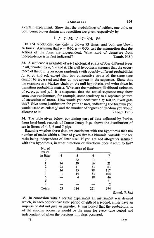
EXERCISES 193
a certain experiment. Show that the probabilities of neither, one only, orboth being blown during any repetition are given respectively by
1-p-q+Pq, p+q-2pq, pq.In 154 repetitions, one only is blown 93 times, and both are blown-
36 times. Assuming that p = 0.60, q = 0.50, test the assumption that theactions of the fuses are independent. What kind of departure fromindependence is in fact indicated? (Camb. N.S.)
33. A sequence is available of n + 1 geological strata of four different typesin all, denoted by a, b, c and d. The null hypothesis assumes that the occur-rence of the four types occur randomly (with possibly different probabilitiesPa, Pt,, p. and pa), except that two consecutive strata of the same typecannot be separated and thus do not appear in the sequence. Show thatthe sequence is a Markov chain on the null hypothesis, and write down itstransition probability matrix. What are the maximum likelihood estimatesof pa, Pb, pa and pa? It is suspected that the actual sequence may showsome non-randomness, for example, some tendency to a repeated patternof succession of states. How would you construct a X2 test to investigatethis? Give some justification for your answer, indicating the formula youwould use to calculate x2 and the number of degrees of freedom you wouldallocate to it. (Lond. Dip.)
34. The table given below, containing part of data collected by Parkesfrom herd-book records of Duroc-Jersey Pigs, shows the distribution ofsex in litters of 4, 5, 6 and 7 pigs.
Examine whether these data are consistent with the hypothesis that thenumber of males within a litter of given size is a binomial variable, the sexratio being independent of litter size. If you are not altogether satisfiedwith this hypothesis, in what direction or directions does it seem to fail?
No. of Size of littermales
in litter 4 5 6 70 1 22 3 -1 14 20 16 21
2 23 41 53 633 14 35 78 1174 1 14 53 1045 - 4 18 466 - - - 217 - - - 2
Totals 53 116 221 374(Lond. B.Sc.)
35. In connexion with a certain experiment an instrument was devisedwhich, in each consecutive time period of Ath of a second, either gave animpulse or did not give an impulse. It was hoped that the probability, p,of the impulse occurring would be the same for every time period andindependent of when the previous impulses occurred.
13 L S II
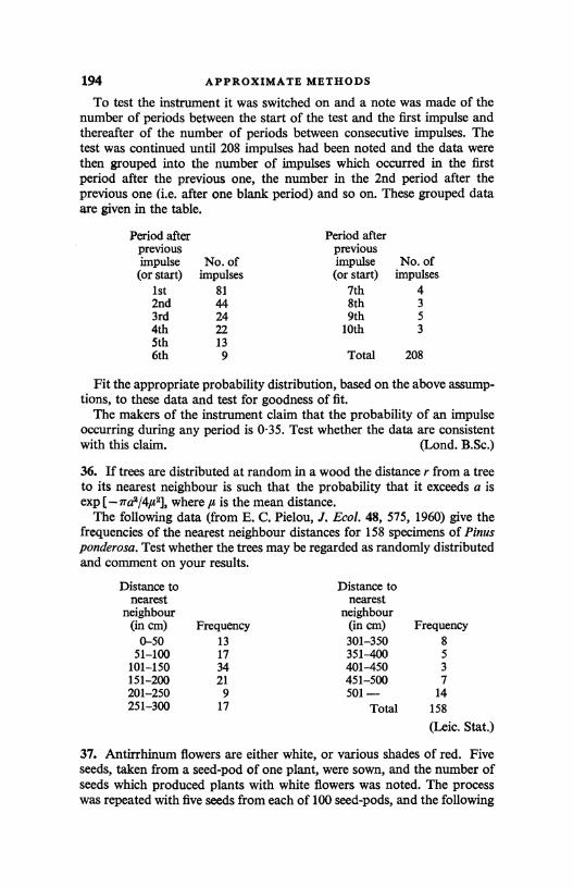
194 APPROXIMATE METHODS
To test the instrument it was switched on and a note was made of thenumber of periods between the start of the test and the first impulse andthereafter of the number of periods between consecutive impulses. Thetest was continued until 208 impulses had been noted and the data werethen grouped into the number of impulses which occurred in the firstperiod after the previous one, the number in the 2nd period after theprevious one (i.e. after one blank period) and so on. These grouped dataare given in the table.
Period after Period afterprevious previous
impulse No. of impulse No. of(or start) impulses (or start) impulses
1st 81 7th 42nd 44 8th 3
3rd 24 9th 5
4th 22 10th 3
5th 13
6th 9 Total 208
Fit the appropriate probability distribution, based on the above assump-tions, to these data and test for goodness of fit.
The makers of the instrument claim that the probability of an impulseoccurring during any period is 0.35. Test whether the data are consistentwith this claim. (Lond. B.Sc.)
36. If trees are distributed at random in a wood the distance r from a treeto its nearest neighbour is such that the probability that it exceeds a isexp [ - ira'/4µx], where ,a is the mean distance.
The following data (from E. C. Pielou, J. Ecol. 48, 575, 1960) give thefrequencies of the nearest neighbour distances for 158 specimens of Pinusponderosa. Test whether the trees may be regarded as randomly distributedand comment on your results.
Distance to Distance tonearest nearest
neighbour neighbour(in cm) Frequency (in cm) Frequency0-50 13 301-350 8
51-100 17 351-400 5
101-150 34 401-450 3
151-200 21 451-500 7201-250 9 501 - 14
251-300 17 Total 158
(Leic. Stat.)
37. Antirrhinum flowers are either white, or various shades of red. Fiveseeds, taken from a seed-pod of one plant, were sown, and the number ofseeds which produced plants with white flowers was noted. The processwas repeated with five seeds from each of 100 seed-pods, and the following
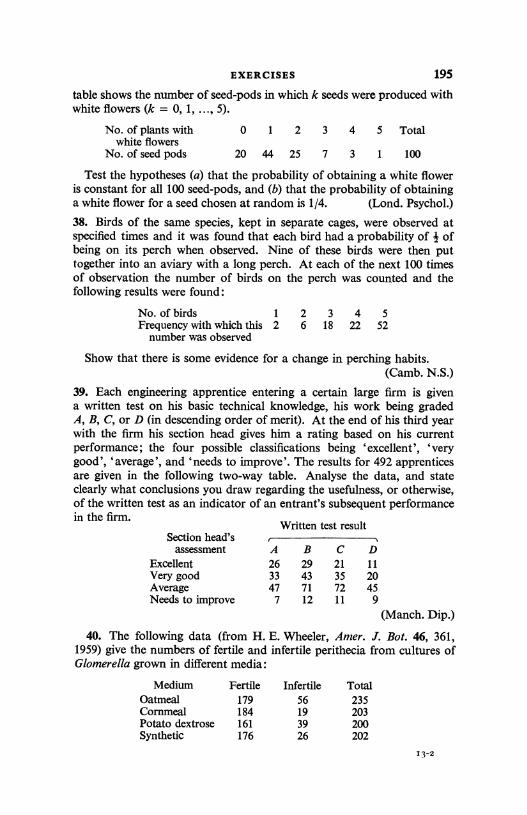
EXERCISES 195
table shows the number of seed-pods in which k seeds were produced withwhite flowers (k = 0, 1, ..., 5).
No. of plants withwhite flowers
0 1 2 3 4 5 Total
No. of seed pods 20 44 25 7 3 1 100
Test the hypotheses (a) that the probability of obtaining a white floweris constant for all 100 seed-pods, and (b) that the probability of obtaininga white flower for a seed chosen at random is 1/4. (Lond. Psychol.)
38. Birds of the same species, kept in separate cages, were observed atspecified times and it was found that each bird had a probability of I ofbeing on its perch when observed. Nine of these birds were then puttogether into an aviary with a long perch. At each of the next 100 timesof observation the number of birds on the perch was counted and thefollowing results were found:
No. of birds 1 2 3 4 5Frequency with which this
number was observed2 6 18 22 52
Show that there is some evidence for a change in perching habits.(Camb. N.S.)
39. Each engineering apprentice entering a certain large firm is givena written test on his basic technical knowledge, his work being gradedA, B, C, or D (in descending order of merit). At the end of his third yearwith the firm his section head gives him a rating based on his currentperformance; the four possible classifications being `excellent', `verygood', `average', and `needs to improve'. The results for 492 apprenticesare given in the following two-way table. Analyse the data, and stateclearly what conclusions you draw regarding the usefulness, or otherwise,of the written test as an indicator of an entrant's subsequent performancein the firm.
Written test result
Secti h ad'son eassessment A B C D
Excellent 26 29 21 11
Very good 33 43 35 20Average 47 71 72 45Needs to improve 7 12 11 9
(Manch. Dip.)
40. The following data (from H. E. Wheeler, Amer. J. Bot. 46, 361,1959) give the numbers of fertile and infertile perithecia from cultures ofGlomerella grown in different media:
Medium Fertile Infertile TotalOatmeal 179 56 235Cornmeal 184 19 203Potato dextrose 161 39 200Synthetic 176 26 202
13-2
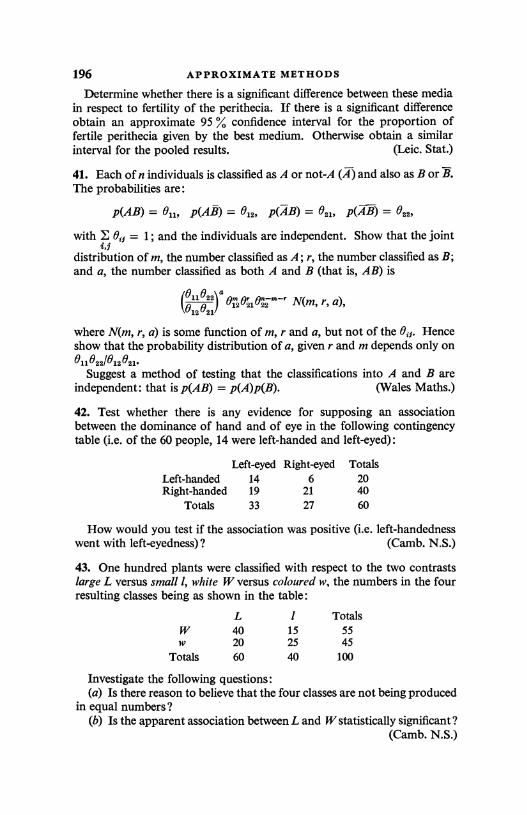
196 APPROXIMATE METHODS
Determine whether there is a significant difference between these mediain respect to fertility of the perithecia. If there is a significant differenceobtain an approximate 95 Y. confidence interval for the proportion offertile perithecia given by the best medium. Otherwise obtain a similarinterval for the pooled results. (Leic. Stat.)
41. Each of n individuals is classified as A or not-A (A) and also as B or B.The probabilities are:
P(AB) = 811, P(AB) = 012, P(AB) = 021, P(AB) = 022,
with E Bij = 1; and the individuals are independent. Show that the jointi,9
distribution of m, the number classified as A; r, the number classified as B;and a, the number classified as both A and B (that is, AB) is
011022 a012021022 m T N(m, r, a),12021)
where N(m, r, a) is some function of m, r and a, but not of the Oil. Henceshow that the probability distribution of a, given r and m depends only on011022/012021
Suggest a method of testing that the classifications into A and B areindependent: that is p(AB) = p(A)p(B). (Wales Maths.)
42. Test whether there is any evidence for supposing an associationbetween the dominance of hand and of eye in the following contingencytable (i.e. of the 60 people, 14 were left-handed and left-eyed):
Left-eyed Right-eyed TotalsLeft-handed 14 6 20Right-handed 19 21 40
Totals 33 27 60
How would you test if the association was positive (i.e. left-handednesswent with left-eyedness)? (Camb. N.S.)
43. One hundred plants were classified with respect to the two contrastslarge L versus small 1, white W versus coloured w, the numbers in the fourresulting classes being as shown in the table:
L 1 TotalsW 40 15 55
w 20 25 45
Totals 60 40 100
Investigate the following questions:(a) Is there reason to believe that the four classes are not being produced
in equal numbers?(b) Is the apparent association between L and W statistically significant?
(Camb. N.S.)
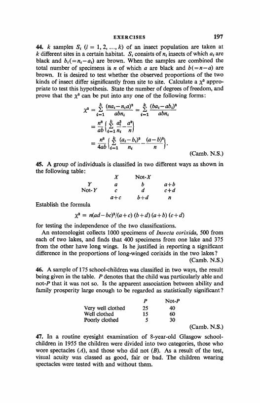
EXERCISES 197
44. k samples Si (i = 1, 2, ..., k) of an insect population are taken atk different sites in a certain habitat. Si consists of n2 insects of which a, areblack and b, (= n; - a .) are brown. When the samples are combined thetotal number of specimens is n of which a are black and b(=n-a) arebrown. It is desired to test whether the observed proportions of the twokinds of insect differ significantly from site to site. Calculate a x2 appro-priate to test this hypothesis. State the number of degrees of freedom, andprove that the x2 can be put into any one of the following forms:
x2 = k (na;-n{a)2 = (ba{-abj2z=1 abn, i=i abn{ns k a, a2l
- nl
n2((
k (a{-b{)2 (a - b)214ab li=1 ni - n )
(Camb. N.S.)
45. A group of individuals is classified in two different ways as shown inthe following table:
X Not-XY a b a+b
Not-Y c d c+da+c b+d n
Establish the formula
x2 = n(ad-bc)2/(a+c) (b+d) (a+b) (c+d)
for testing the independence of the two classifications.An entomologist collects 1000 specimens of Insecta corixida, 500 from
each of two lakes, and finds that 400 specimens from one lake and 375from the other have long wings. Is he justified in reporting a significantdifference in the proportions of long-winged corixids in the two lakes?
(Camb. N.S.)
46. A sample of 175 school-children was classified in two ways, the resultbeing given in the table. P denotes that the child was particularly able andnot-P that it was not so. Is the apparent association between ability andfamily prosperity large enough to be regarded as statistically significant?
P Not-PVery well clothed 25 40Well clothed 15 60Poorly clothed 5 30
(Camb. N.S.)
47. In a routine eyesight examination of 8-year-old Glasgow school-children in 1955 the children were divided into two categories, those whowore spectacles (A), and those who did not (B). As a result of the test,visual acuity was classed as good, fair or bad. The children wearingspectacles were tested with and without them.
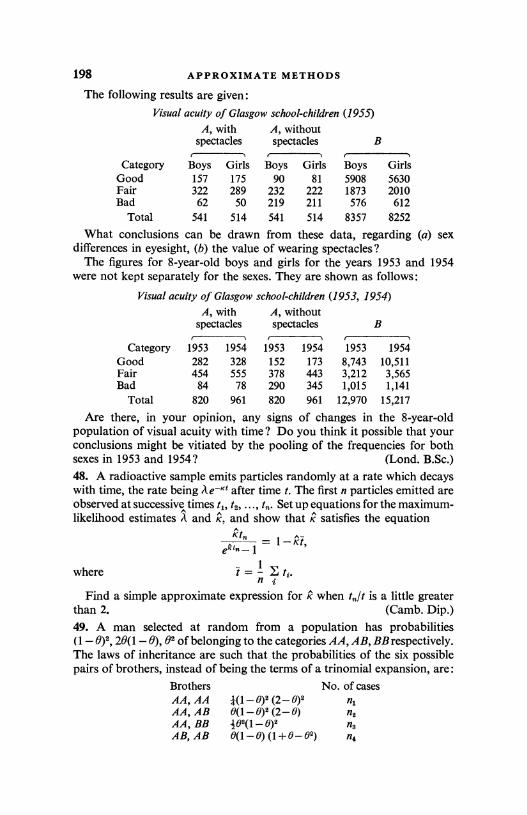
198 APPROXIMATE METHODS
The following results are given:
Visual acuity of Glasgow school-children (1955)A, with
spectacles
A, withoutspectacles B
Category Boys Girls Boys Girls Boys GirlsGood 157 175 90 81 5908 5630Fair 322 289 232 222 1873 2010Bad 62 50 219 211 576 612
Total 541 514 541 514 8357 8252
What conclusions can be drawn from these data, regarding (a) sexdifferences in eyesight, (b) the value of wearing spectacles?
The figures for 8-year-old boys and girls for the years 1953 and 1954were not kept separately for the sexes. They are shown as follows:
Visual acuity of Glasgow school-children (1953, 1954)A, with
spectacles
A, withoutspectacles B
Category 1953 1954 1953 1954 1953 1954
Good 282 328 152 173 8,743 10,511Fair 454 555 378 443 3,212 3,565Bad 84 78 290 345 1,015 1,141
Total 820 961 820 961 12,970 15,217
Are there, in your opinion, any signs of changes in the 8-year-oldpopulation of visual acuity with time? Do you think it possible that yourconclusions might be vitiated by the pooling of the frequencies for bothsexes in 1953 and 1954? (Lond. B.Sc.)48. A radioactive sample emits particles randomly at a rate which decayswith time, the rate being Ae-"t after time t. The first n particles emitted areobserved at successive times t1, t2i ..., t,,. Set up equations for the maximum-likelihood estimates A and K. and show that a satisfies the equation
Kt n_ekt"-1 = 1-Kt,
where i = 1 E tt.n i
Find a simple approximate expression for K when is a little greaterthan 2. (Camb. Dip.)49. A man selected at random from a population has probabilities(1 - 0)2, 20(1- 0), 02 of belonging to the categories AA, AB, BBrespectively.The laws of inheritance are such that the probabilities of the six possiblepairs of brothers, instead of being the terms of a trinomial expansion, are:
Brothers No. of casesAA, AA 1(1- 0)2 (2- 0)2 nlAA, AB 6(1-0)2 (2-0) n2AA, BB 02(1 - 0)2 n2
AB, AB 0(1-0) (1+0-92) n`
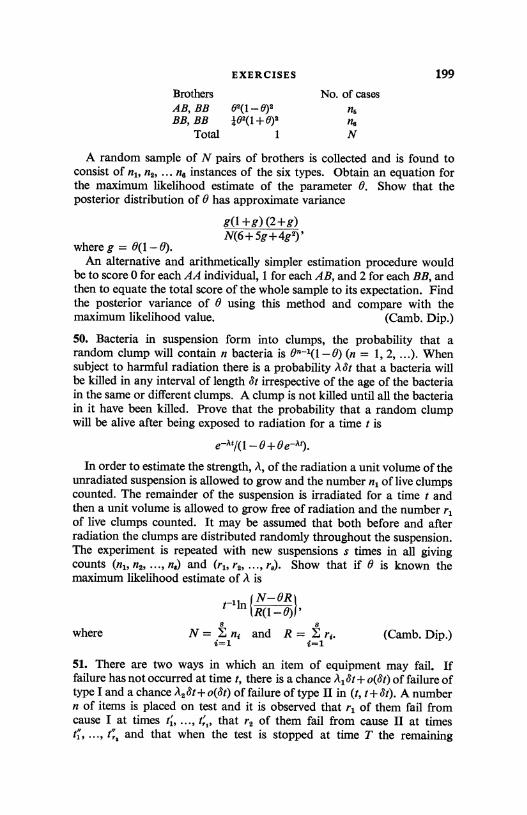
EXERCISES 199
Brothers No. of cases
AB, BB 02(1-0)2 nb
BB, BB *02(1 + 0)2 ne
Total 1 N
A random sample of N pairs of brothers is collected and is found toconsist of n,, n2, ... n6 instances of the six types. Obtain an equation forthe maximum likelihood estimate of the parameter 0. Show that theposterior distribution of 0 has approximate variance
where g = 0(1- 0).
g(1 +g) (2+g)N(6 + 5g+4g2)'
An alternative and arithmetically simpler estimation procedure wouldbe to score 0 for each AA individual, I for each AB, and 2 for each BB, andthen to equate the total score of the whole sample to its expectation. Findthe posterior variance of 0 using this method and compare with themaximum likelihood value. (Camb. Dip.)
50. Bacteria in suspension form into clumps, the probability that arandom clump will contain n bacteria is 0n-1(1-0) (n = 1, 2, ...). Whensubject to harmful radiation there is a probability A8t that a bacteria willbe killed in any interval of length St irrespective of the age of the bacteriain the same or different clumps. A clump is not killed until all the bacteriain it have been killed. Prove that the probability that a random clumpwill be alive after being exposed to radiation for a time t is
e-21110 -0+0e-A9.
In order to estimate the strength, A, of the radiation a unit volume of theunradiated suspension is allowed to grow and the number n, of live clumpscounted. The remainder of the suspension is irradiated for a time t andthen a unit volume is allowed to grow free of radiation and the number r,of live clumps counted. It may be assumed that both before and afterradiation the clumps are distributed randomly throughout the suspension.The experiment is repeated with new suspensions s times in all givingcounts (n,, n2, ..., n,) and (r,, r2, ..., re). Show that if 0 is known themaximum likelihood estimate of A is
t-11n N- OR lIR(1-B)1'
8 8where N= E n; and R = E r1. (Camb. Dip.)
i=1 i=1
51. There are two ways in which an item of equipment may fail. Iffailure has not occurred at time t, there is a chance A,St+ o(St) of failure oftype I and a chance A28t+o(8t) of failure of type II in (t, t+&t). A numbern of items is placed on test and it is observed that r, of them fail fromcause I at times ti, ..., t;,, that r2 of them fail from cause II at timesti, ..., t:, and that when the test is stopped at time T the remaining
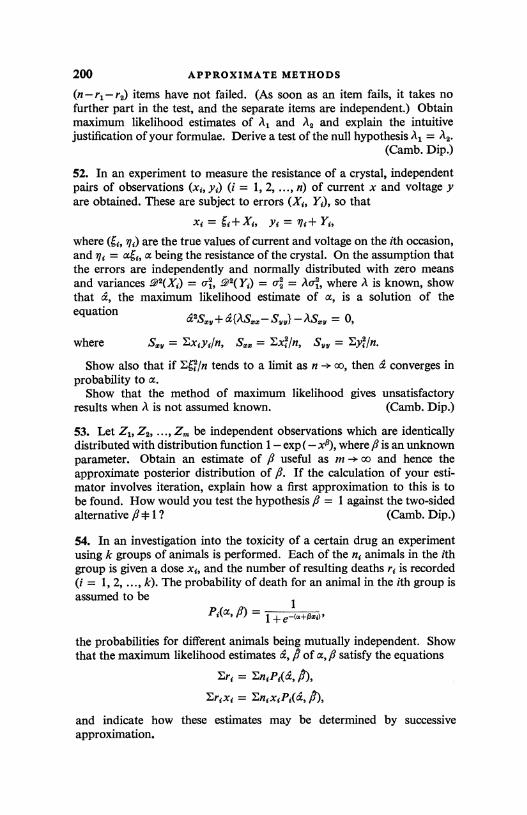
200 APPROXIMATE METHODS
(n - rl - r2) items have not failed. (As soon as an item fails, it takes nofurther part in the test, and the separate items are independent.) Obtainmaximum likelihood estimates of Al and A2 and explain the intuitivejustification of your formulae. Derive a test of the null hypothesis Al = 112
(Camb. Dip.)
52. In an experiment to measure the resistance of a crystal, independentpairs of observations (xi, yi) (i = 1, 2, ..., n) of current x and voltage yare obtained. These are subject to errors (Xi, Yi), so that
xi = 6i+ Xi, yi = I,+ I t,where (6i, q,) are the true values of current and voltage on the ith occasion,and ,ii = a6i, a being the resistance of the crystal. On the assumption thatthe errors are independently and normally distributed with zero meansand variances _ 9 2 ( X i ) = o , 92(Yi) = a2 = Ao L, where A is known, showthat a, the maximum likelihood estimate of a, is a solution of theequation
CG2Sxy+CG{)(,sxx-,Syv}-ASxv = 0,
where Sx = Exiyil n, S.. = Ex, In, Sv = Ey /n.
Show also that if Z 6,2/n tends to a limit as n oo, then a converges inprobability to a.
Show that the method of maximum likelihood gives unsatisfactoryresults when d is not assumed known. (Camb. Dip.)
53. Let Zi, Z2, ..., Z. be independent observations which are identicallydistributed with distribution function 1- exp (- xs), where ft is an unknownparameter. Obtain an estimate of ft useful as m -+ oo and hence theapproximate posterior distribution of ft. If the calculation of your esti-mator involves iteration, explain how a first approximation to this is tobe found. How would you test the hypothesis,B = I against the two-sidedalternative f * 1 ? (Camb. Dip.)
54. In an investigation into the toxicity of a certain drug an experimentusing k groups of animals is performed. Each of the ni animals in the ithgroup is given a dose xi, and the number of resulting deaths ri is recorded(i = 1, 2, ..., k). The probability of death for an animal in the ith group isassumed to be I
Pi(a, Q) = 1 + e c-+Rxd'
the probabilities for different animals being mutually independent. Showthat the maximum likelihood estimates a, A of a,,8 satisfy the equations
Eri = EniPi(d, fi),
Erixi = EnixiPi(a, ft),
and indicate how these estimates may be determined by successiveapproximation.
EXERCISES 201
Show also that the asymptotic variances and covariances of the posteriordistribution of a and are given by
/_' 2(a) _ (l/F'wi)+(X2/SS), g2(ft) = 1/Sxx,
le(a, N) = -XISxx,
where wi = nipi(&, A) [1-Pi(&, J3)],
g = ZwiX/F-'wi, S.. = F'wi(Xi-X)2
Hence obtain a large sample test of the hypothesis that -a/fl, the mean ofthe tolerance distribution associated with Pi(a, fi), has a specified value µo,and derive a 95 % large sample confidence interval for -a//i.
(Camb. Dip.)
55. Show that the probability of needing exactly k independent trials toobtain a given number n of successes, when each trial can result in successor failure and the chance of success is p for all trials, is
k- 1\n-11 pngk-n'
where q = 1-p. Writing k = n + s, show that the mean and variance of sare nq/p and nq/p2.
Two such sequences of trials were carried out in which the requirednumbers of successes were nl and n2, and the numbers of trials neededwere nl+sl and n2+s2. Two estimates were proposed for the mean numberof failures per success; the first was the total number of failures divided bythe total number of successes, and the second was the average of thenumbers of failures per success in the two sequences. Which estimatewould you prefer? State your reasons carefully. (Camb. N.S.)
56. A subject answers n multiple-choice questions, each having k possibleanswers, and obtains R correct answers. Suppose that the subject reallyknows the answers to v of the questions, where v is an unknown parameter,and that his answers to the remaining n - v questions are pure guesses,each having a probability 1 /k of being correct. Write down the probabilitydistribution of R, indicating its relation to the binomial distribution.
If B is the probability that he knows the correct answer and has priordistribution B0(a, b), and. if the questions are answered independentlydiscuss the posterior distribution of 0 given R. (Lond. B.Sc.)
57. An estimate is required of the number of individuals in a largepopulation of size N, who possess a certain attribute A. Two methods areproposed. Method I would select a random sample of size aN and inter-view each member of the sample to determine whether he possesses A ornot. Method II would send out the postal question `Do you possess ATto all N individuals and then, in order to avoid any possible bias due to
202 APPROXIMATE METHODS
misunderstanding of the question, etc., would interview a random sampleof size aN,, of those Ny individuals who replied `Yes' and a randomsample of size aN of those N. individuals who replied `No'.
Assuming that, if method II were used, all N individuals would reply tothe question, suggest estimates for the two methods in terms of the resultsof the interviews. If pv(=1-qv) is the proportion of the yes-replyingindividuals who actually have A, and 1-q,,) is the proportion of theno-replying individuals who actually have A, show that the variances ofthe estimates for methods I and II are
(N,,p.y+Nnp.) (N q +Nngn) and N1Pvq +NnpnqNa a
respectively.Show that method II has the smaller variance. Discuss the relevance of
these sample variances to the posterior distribution of the number in thepopulation possessing A. (Wales Dip.)
203
8
LEAST SQUARES
The method of least squares is a method of investigating thedependence of a random variable on other quantities. Closelyassociated with the method is the technique of analysis of vari-ance. We begin with a special case and later turn to moregeneral theory. The reader is advised to re-read the section onthe multivariate normal distribution in § 3.5 before reading § 8.3.
8.1. Linear homoscedastic normal regressionWe are interested in the dependence of one random variable y
on another random variable x. We saw in §3.2 that this couldmost easily be expressed in terms of the distribution of x and theconditional distribution of y, given x. These distributions willdepend on parameters; suppose the dependence is such that
p(x,Y10, 0) = p(x10)p(YI x, 0); (1)
that is, the parameters in the two distributions are distinct.Then this is effectively equation 5.5.21 again with x = (x, y)and t(x) = x. As explained in § 5.5, and illustrated in provingtheorem 7.6.2, if 0 and 0 have independent prior distributions,inferences about the conditional distribution may be made bysupposing x to be fixed. We shall make these two assumptions((1) and the prior independence of 0 and ¢) throughout thissection, and use more general forms of them in later sections.Consequently all our results will be stated for fixed x. Providedthe assumptions obtain, they are equally valid for random x.Linear homoscedastic normal regression has already beendefined (equations 3.2.13 and 14).
Theorem 1. If x = (x1i x2, ..., xn) is a set of real numbers, and if,for fixed x, the random variables Y1, Y2, ..., yn are independentnormal random variables with
d'(Yi I x) = a +,6(xi - (2)
204 LEAST SQUARES [8.1
and 92(YZ I x) = 0 (3)
(i = 1, 2, ..., n) ; then if the prior distributions of a, 6 and In 0 areindependent and uniform:
(i) the posterior distribution of
(/3 - b)/{S2/Sxx(n - 2)}1 (4)
is a t-distribution with (n - 2) degrees of freedom;(ii) the posterior distribution of
(a - a)/{S2/n(n - 2)}i (5)
is a t-distribution with (n - 2) degrees of freedom;(iii) the posterior distribution of
S2/0 (6)
is x2 with (n - 2) degrees of freedom.The notation used in (4), (5) and (6) is
Sxx = E(x1- x)2, Sx = E(x1- x) (Y1-Y),
S = E(Y1-Y)2, Jr
(7)
S2 = Svv-SxlA xx (8)
and a = y, b = Sxv/Sxx. (9)
The likelihood of the y's, given the x's, is
p(y I x, a, fl, 0) cc O-In exp [ - {Y1- a - /3(x1 x)}2/20i=1
and hence the joint posterior distribution of a, f and 0 is
(10)
n(a, x, y) a q-lcn+2) exp[ - {y; - a - /3(x1- x)}2/2c ] .
1=i(11)
The sum of squares in the exponential may be written as
E{(y, -Y) + (y - a) - R(x1- x)}2
= Svv+n(y-a)2+/32Sxx-2NSxv
= Svv-SxvISxx+n(Y-a)2+Sxx(R-Sxv/Sxx)2
= S2 + n(a - a)2 + Sxx(ft - b)2, (12)
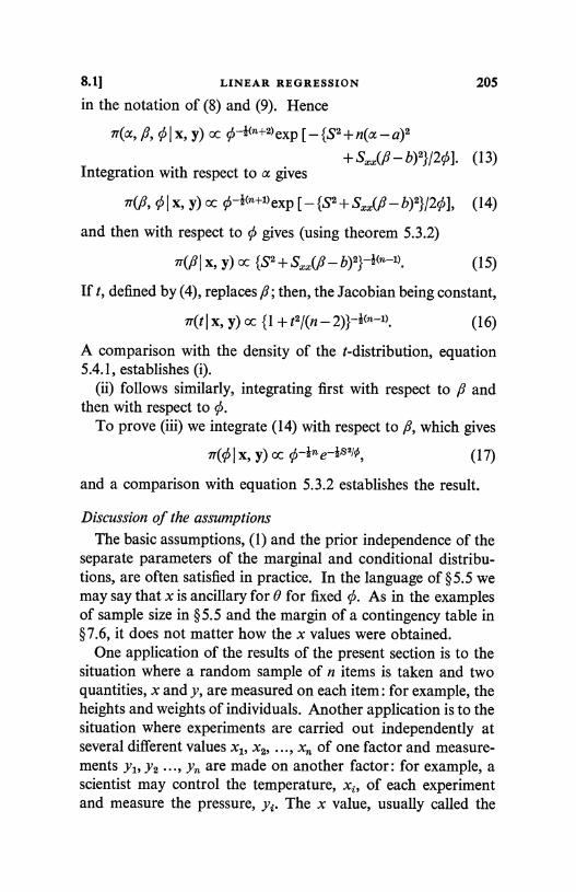
8.1] LINEAR REGRESSION
in the notation of (8) and (9). Hence
ir(a, i, 01 X, y) a 0-I1n+21 exp [ - {S2 + n(a - a)2
Integration with respect to a gives
205
+ SS.(f - b)2}/201. (13)
ir(fl, 01 x, y) cc 0-Icn+1) exp [ - {S2 + b)2}/2cb], (14)
and then with respect to 0 gives (using theorem 5.3.2)
7T('61X, y) cc {S2 + Sxx(Q - b)2}-Icn-1). (15)
If t, defined by (4), replaces /3; then, the Jacobian being constant,
7T(t I X, y) cc {l + t2/(n - 2)}-I(n-1)(16)
A comparison with the density of the t-distribution, equation5.4.1, establishes (i).
(ii) follows similarly, integrating first with respect to ,6 andthen with respect to 0.
To prove (iii) we integrate (14) with respect to fl, which gives
7T(o I X, y) OC 0-In e-11'10, (17)
and a comparison with equation 5.3.2 establishes the result.
Discussion of the assumptions
The basic assumptions, (1) and the prior independence of theseparate parameters of the marginal and conditional distribu-tions, are often satisfied in practice. In the language of § 5.5 wemay say that x is ancillary for 0 for fixed ¢. As in the examplesof sample size in § 5.5 and the margin of a contingency table in§ 7.6, it does not matter how the x values were obtained.
One application of the results of the present section is to thesituation where a random sample of n items is taken and twoquantities, x and y, are measured on each item: for example, theheights and weights of individuals. Another application is to thesituation where experiments are carried out independently atseveral different values x1, x2, ..., xn of one factor and measure-ments Y1, Y2 ..., yn are made on another factor: for example, ascientist may control the temperature, x17 of each experimentand measure the pressure, yj. The x value, usually called the
206 LEAST SQUARES [8.1
independent variable, is different in the two cases: in the formerit is a random variable, in the latter it is completely under thecontrol of the experimenter. Nevertheless, the same analysis ofthe dependence of y on x applies in both cases. The y variable isusually called the dependent variable. The reader should becareful not to confuse the use of the word `independent' herewith its use in the phrase `one random variable is independentof another'.
The form of the conditional distribution assumed in theorem 1is that discussed in § 3.2. The distributions are normal and there-fore can be completely described by their means and variances.The means are supposed linear in the independent variable andthe variances are constant (homoscedastic). (Notice that we havewritten the regression in (2) in a form which is slightly differentfrom equation 3.2.13, the reason for which will appear below:essentially, a of 3.2.13 has been rewritten a -/3x.) It is importantthat the assumptions of linearity and homoscedasticity shouldbe remembered when making any application of the theorem.Too often regression lines are fitted by the simple methods ofthis section without regard to this point. An example of alterna-tive methods of investigating the dependence of y on x withoutinvoking them will be discussed below. Particular attentionattaches to the case 8 = 0, when the two variables are inde-pendent and there is said to be no regression effect. A test ofthis null hypothesis will be developed below (table 8.1).
The prior distributions of a and 0 are as usual: 0 is a varianceand a = n-1Ecf(y2 I x); that is, the expectation of y averaged overthe values of x used in the experiment. We have chosen f, whichis the only parameter that expresses any dependence of y on x, tobe uniformly distributed: this is to be interpreted in the sense of§ 5.2, merely meaning that the prior knowledge of /3 is so diffusethat the prior density is sensibly constant over the effective rangeof the likelihood function. It has been supposed independent ofa and ¢ because it will typically be reasonable to suppose thatknowledge of the expectation and/or the variance of y (that is,of a and/or 0) will not alter one's knowledge of the dependenceof y on x (that is, of /3).
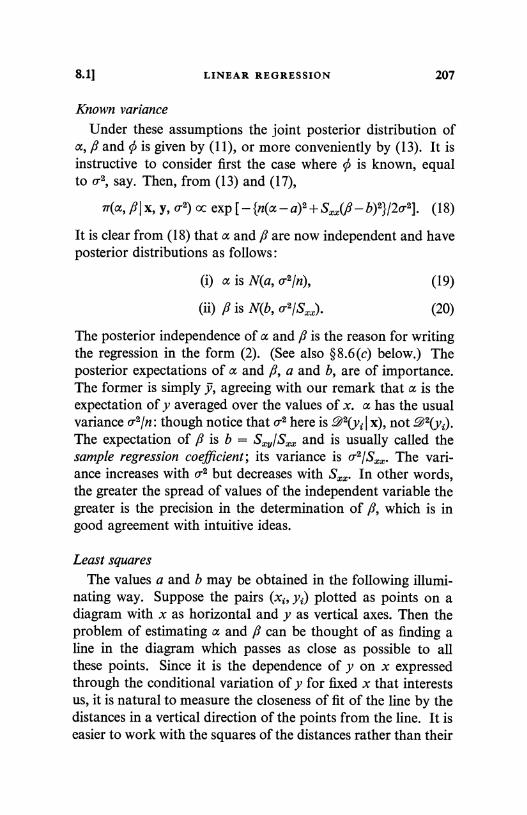
8.11 LINEAR REGRESSION 207
Known variance
Under these assumptions the joint posterior distribution ofa, /3 and 0 is given by (11), or more conveniently by (13). It isinstructive to consider first the case where 0 is known, equalto 0.2, say. Then, from (13) and (17),
2r(a, Q I x, y, v2) cc exp [ - {n(a - a)2 + Sxx(ft - b)2}/20.2] (18)
It is clear from (18) that a and 8 are now independent and haveposterior distributions as follows:
(i) a is N(a, O'2/n), (19)
(ii) f3 is N(b, o2/SS.). (20)
The posterior independence of a and 6 is the reason for writingthe regression in the form (2). (See also §8.6(c) below.) Theposterior expectations of a and f, a and b, are of importance.The former is simply y, agreeing with our remark that a is theexpectation of y averaged over the values of x. a has the usualvariance 0-2/n: though notice that o-2 here is .92(y, I x), not .92(y,).The expectation of fl is b = and is usually called thesample regression coefficient; its variance is v2/Sxx. The vari-ance increases with 0.2 but decreases with S,,,;. In other words,the greater the spread of values of the independent variable thegreater is the precision in the determination of ft, which is ingood agreement with intuitive ideas.
Least squares
The values a and b may be obtained in the following illumi-nating way. Suppose the pairs (xi, yZ) plotted as points on adiagram with x as horizontal and y as vertical axes. Then theproblem of estimating a and ft can be thought of as finding aline in the diagram which passes as close as possible to allthese points. Since it is the dependence of y on x expressedthrough the conditional variation of y for fixed x that interestsus, it is natural to measure the closeness of fit of the line by thedistances in a vertical direction of the points from the line. It iseasier to work with the squares of the distances rather than their
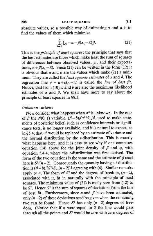
208 LEAST SQUARES [8.1
absolute values, so a possible way of estimating a and ft is tofind the values of them which minimize
nE [yi-a-/3(xi-x)]2. (21)i=1
This is the principle of least squares: the principle that says thatthe best estimates are those which make least the sum of squaresof differences between observed values, yi, and their expecta-tions, a+f(xi-x). Since (21) can be written in the form (12) itis obvious that a and b are the values which make (21) a mini-mum. They are called the least squares estimates of a and ft. Theregression line y = a+ b(x -x) is called the line of best fit.Notice, that from (10), a and b are also the maximum likelihoodestimates of a and f. We shall have more to say about theprinciple of least squares in § 8.3.
Unknown varianceNow consider what happens when o 2 is unknown. In the case
of /3 the N(0, 1) variable, (/t-b)/(o.2/Sxx)1, used to make state-ments of posterior belief, such as confidence intervals or signifi-cance tests, is no longer available, and it is natural to expect, asin § 5.4, that .2 would be replaced by an estimate of variance andthe normal distribution by the t-distribution. This is exactlywhat happens here, and it is easy to see why if one comparesequation (14) above for the joint density of /t and 0, withequation 5.4.4, where the t-distribution was first derived. Theform of the two equations is the same and the estimate of ¢ usedhere is S2/(n - 2). Consequently the quantity having a t-distribu-tion is (f - b)/{S2/Sxx(n - 2)}1 agreeing with (4). Similar remarksapply to a. The form of S2 and the degrees of freedom, (n - 2),associated with it, fit in naturally with the principle of leastsquares. The minimum value of (21) is easily seen from (12) tobe S2. Hence S2 is the sum of squares of deviations from the lineof best fit. Furthermore, since a and ft have been estimated,only (n - 2) of these deviations need be given when the remainingtwo can be found. Hence S2 has only (n-2) degrees of free-dom. (Notice that if n were equal to 2 the line would passthrough all the points and S2 would be zero with zero degrees of
8.11 LINEAR REGRESSION 209
freedom.) According to the principle of least squares the esti-mate of variance is obtained by dividing the minimum of thesum of squares (called the residual sum of squares) by the numberof observations less the number of parameters, apart from ¢,estimated, here 2. Notice that the maximum likelihood estimateof 0 is S2/n.
In view of the close connexion between equations (14) and5.4.4 it is clear that the posterior distribution of 0 will be relatedto that of x2 in the usual way. This is expressed in part (iii) oftheorem 1. As usual, the degrees of freedom will be the same asthose of t, namely (n - 2).
Significance tests
Confidence intervals and significance tests for any of the para-meters will follow in the same way as they did in chapter 5. Forexample, a 95 % confidence interval- for /3 is (cf. equation 5.4.9),with s = 0.025,
b - t6(n - 2) S/{Sxx(n - 2)}i 5 /3 < b + t6(n - 2) S/(Sxx(n - 2#. (22)
The significance test for /3 = 0; that is, for independence of xand y, can be put into an interesting form. The test criterion is(4), with /3 = 0, and since the t-distribution is symmetrical wecan square it and refer
b2 _ Sxv/SX (23)S21Sxx(n-2) [Svv-Sxvlsxx]l(n-2)
to values of t,2(n - 2). (The alternative form follows from (8)and (9).) Now 7
Svv = [Svv - Sxvl Sxxl + [Sxvl Sxx] (24)
The left-hand side is the total sum of squares for the y's. Thefirst bracket on the right is the residual sum of squares and also,when divided by (n - 2), the denominator of (23). The secondbracket is the numerator of (23) and will be called the sum ofsquares due to regression. Furthermore, since (§6.2) t2 is equalto F with 1 and (n - 2) degrees of freedom, we can write thecalculations in the form of an analysis of variance table (§6.5)
t To avoid confusion between the average expectation of yt and the significancelevel, e, instead of a, has been used for the latter.
14 LS 11
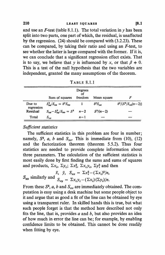
210 LEAST SQUARES [8.1
and use an F -test (table 8.1.1). The total variation in y has beensplit into two parts, one part of which, the residual, is unaffectedby the regression. (24) should be compared with (3.2.23). Thesecan be compared, by taking their ratio and using an F-test, tosee whether the latter is large compared with the former. If it is,we can conclude that a significant regression effect exists. Thatis to say, we believe that y is influenced by x, or that 6 + 0.This is a test of the null hypothesis that the two variables areindependent, granted the many assumptions of the theorem.
TABLE 8.1.1
Sum of squares
Degreesof
freedom Mean square FDue to b'Sxx 1 bBSxz bE/{S$/Sxx(n-2)}regression
Residual SE n-2 S'/(n-2) -Total Si,,, n-1 - --
Sufficient statisticsThe sufficient statistics in this problem are four in number;
namely, SO, a, b and S. This is immediate from (10), (12)and the factorization theorem (theorem 5.5.2). Thus fourstatistics are needed to provide complete information aboutthree parameters. The calculation of the sufficient statistics ismost easily done by first finding the sums and sums of squaresand products, Exi, Eyi; Exg, Exiyi, Eye and then
x, y, S.. = Exi - (Exi)t/n,Sv similarly and S., = Exi yi - (Exi) (Eyi)/n.
From these S$, a, b and S.,., are immediately obtained. The com-putation is easy using a desk machine but some people object toit and argue that as good a fit of the line can be obtained by eyeusing a transparent ruler. In skilled hands this is true, but whatsuch people forget is that the method here described not onlyfits the line, that is, provides a and b, but also provides an ideaof how much in error the line can be; for example, by enablingconfidence limits to be obtained. This cannot be done readilywhen fitting by eye.
8.1] LINEAR REGRESSION 211
Posterior distribution of the conditional expectationIt is sometimes necessary to test hypotheses or make confi-
dence statements about quantities other than a, ft or 0 separately.For example, we may require to give limits for the expected valueof y for a given value xo of the independent variable, or to testthe hypothesis that the regression line passes through a givenpoint (xo, yo). These may easily be accomplished by using adevice that was adopted in proving theorem 6.1.3: namely, toconsider the required posterior distribution for fixed 0 and thento average over the known posterior distribution of 0 (equa-tion (6)). In the examples quoted we require the posterior dis-tribution of S(y I x0) = a + /3(xo - x'). Now, given 0 = &2, wesaw in equations (18), (19) and (20) that a and ft were indepen-dent normal variables with means and variances there specified.It follows (theorem 3.5.5) that off(y I xo) is
N[a + b(xo a.2{n-1 + (xo -Hence, by exactly the same argument as was used in provingtheorem 6.1.3, the posterior distribution of .9(y I xo) is such that
S(Y I xo) - a - b(xo - x) (25)[S2{n-1 + (xo - x)2/SS.}/(n - 2)]I
has a t-distribution with (n - 2) degrees of freedom. Confidencelimits for e(y I x0) may be obtained in the usual way, and the nullhypothesis that the line passes through (xo, yo), that is, that,9(Y I x0) = Yo, may be tested by putting e(y I x0) = yo in (25) andreferring the resulting statistic to the t-distribution. Notice thatthe confidence limits derived from (25) will have width propor-tional to the denominator of (25) and will therefore be wider themore x0 deviates from X. It is more difficult to be precise aboutthe line at points distant from x than it is near x; which isintuitively reasonable.
Posterior distribution of the lineIt is possible to make confidence statements about the line
and not merely its value at a fixed value, x0. To do this it isnecessary to find the joint distribution of a and /i. This can be
14-2
212 LEAST SQUARES [8.1
done by integrating (13) with respect to 0. The result will clearlybe a joint density which is constant for values of a and ft forwhich n(a - a)2 + Sxx(/3 - b)2 is constant. To find joint confidencesets for a and f it is therefore only necessary to find the distribu-tion of n(a - a)2 + Sxx(f - b)2. Now a comparison of equation (13)with equation 6.4.8, and the argument that led from the latterto the result concerning the F-distribution, will here show that
[n(a - a)2 + SSx(ft - b)2] /2 (26)S2/(n - 2)
has an F-distribution with 2 and (n - 2) degrees of freedom.This is a special case of a general result to be established later(theorem 8.3.1). The hypothesis that the line has equationy = ao +,80(x -x) may be tested by putting a = ao, 8 = fio in(26) and referring the statistic to the F-distribution.
PredictionAnother problem that often arises in regression theory is that
of predicting the value of the dependent variable for a givenvalue, xo, of the independent variable: a scientist who has experi-mented at values xl, x2, ..., x,,, may wish to estimate what wouldhappen if he were to experiment at xo; or if the independentvariable is time he may wish to predict what will happen at somepoint in the future. To answer this problem we need to havethe density of y given a value xo, the data x, y, and the priorknowledge : that is nr(y I x, y, xo), where reference to the priorknowledge H is, as usual, omitted. To find this, consider first
7T(y I X, Y, x0, a, Q, 0).
This is N(a + f(xo -.9), 0). Also
7T(a I x, y, xo, fl, 0) is N(a, 01n)
(equation (19)). Hence, for fixed x, y, xo, ft and 0; y and ahave a joint normal density (§3.2, in particular equation 3.2.18)and
,T(y I x, y, xo, /3, O) is N[a + f(xo - x), ¢ + ¢/n].
Applying the same argument again to the joint density of y and ffor fixed x, y, xo and 0 we have, since
1T(# I x, y, xo, 0) is N(b, 01S..)
8.11 LINEAR REGRESSION
(equation (20)) that 7r(y I x, y, x0, 0) is
N[a+b(xo-x), 0+q/n+(xo-x)2q5/S].
213
Hence
7T(y I X, Y, x0)
= f rr(Y I X, Y, xo, 0) 7T(01 x, y, xo) do
cc f O-1(n+l)exp C - G
{y - a - b(xo - x)}N+ S2) /20] do
L +n 1+(xo-x)NIS.x
from equation (17). The integration performed in the usual way(compare the passage from (14) to (15)) shows that
y - a - b(xo - x) (27){S2 [I + n-1 + (xo - x)2/SS]/(n - 2)}1
has a t-distribution with (n - 2) degrees of freedom. Hence con-fidence limits]' for y may be found in the usual way. A com-parison of (25) with (27) shows that the limits for y in (27) arewider than those for S(yI x0) in (25) since there is an additionalterm, 1, in the multiplier of the estimate, S2/(n - 2), of residualvariance in the denominator of (27). This is reasonable since yequals d (y I xo) plus an additional term which is N(0, ¢) (cf.equation 3.2.22) : indeed we could have derived (27) by usingthis remark for fixed 0, and then integrating as usual withrespect to 0. Again these limits increase in width as x0 departsfrom X. Remember, too, that these methods are based on theassumption of linear regression which may not hold into thefuture even when it holds over the original range of x-values.
An alternative method
We conclude this section by giving an example of how thedependence of one random variable on an independent variable(random or not) can be investigated without making the assump-tions of linear homoscedastic regression. The method describedis by no means the only possible one. Suppose, for convenience
t Notice that y is not a parameter, so that the definition of a confidenceinterval given in § 5.2 is being extended from the posterior distribution of a para-meter to the posterior distribution of any random variable, here a futureobservation.
214 LEAST SQUARES [8.1
in explanation, that the x-values are chosen by the experimenter.Then the range of x-values may be divided into groups and thenumbers in the groups, ri., say (the reason for the notation willbe apparent in a moment), are fixed numbers chosen by theexperimenter. Suppose the range of y similarly divided intogroups and let r15 be the numbers of observations in both theith-group of x-values and the jth-group of y-values. Then
E ri; = ri. , and ri1 = r. 37 i
is a random variable which is the number in the jth-group ofy-values. Let Oi; be the probabilty of an observation whichbelongs to the ith-group of x-values belonging to the jth-groupof y-values. Then if y is independent of x, Oij does not depend oni and the null hypothesis of independence may be tested by themethods of theorem 7.6.2. If x were a random variable theorem7.6.1 would be needed, but the resulting test will be the same.The group sizes will have to be chosen so that the expectednumbers are sufficiently large for the limiting X2-distribution tobe used as an approximation. In the case of the dependent vari-able this choice, which will have to be made after the results areavailable, will influence the randomness of the r, f. The preciseeffect of this is not properly understood. Fisher and othersclaim that the results of § 7.6 are still valid even if the r. 5, as wellas the r1 , are fixed, but it is not clear from Bayesian argumentsthat this is so. Nevertheless, the effect of fixing the r.5 is likelyto be small and the test can probably be safely applied. Noticethat this test makes no assumptions about linear homoscedasticregression of y on x.
8.2. Correlation coefficientThe topic of this section has nothing to do with least squares
but is included here because of its close relationship to that of theprevious section. The results are not used elsewhere in the book.
Theorem 1. If (x, y) = (x1, yl; x2, Y2; ... ; xn, yn) is a randomsample from a bivariate normal density with ff(xi) = 01,
'(Yi) = 02, -92(xi) = 01, g2(y) = 02 and correlation coefficientp; and if the prior distributions of 01, 02, In q and in O2 are uniform
8.21 CORRELATION COEFFICIENT 215
and independent, and independent of the prior distribution of pwhich nowhere vanishes; then the posterior distribution of p issuch that tanh-1p is approximately (n -> co) normal with
mean: tanh-1r, variance: n-1, (1)
where r = SYY).
If 7T(p) is the prior distribution of p then, in the usual way, thejoint posterior density of 61, 02, 01, 02 and p is proportional to(cf. 3.2.17)
(P)exp 1-2(1-
1n
(X, - 01)2
(c1c2)1n+1(1- p2)}n P2) a.=1 01
_ 2P(xi - 61) (Yi - 02)+-
(Yi -(2)01 02 02
In the usual way we may writey(xi-61)2 = E(xi-x)2+n(x-61)2 = Sxx+n(x-61)2,
in the notation of equation 8.1.7, etc., and (2) becomes
70)-,(___ 1 Sxx _ 2pSxv Svv
(q1 Y )1n+1(1 - p2)1n exp C - 2(1 - p2) 01 0102 + 02_ n J(x-61)2-2P(x-61)
(3)2(1-P2)
l 1 0101 02
The integration with respect to 61 and 02 may now be carried outusing the fact that the normal bivariate density necessarily hasintegral one. Consequently
1, PI X, Y) (12)(1-p2)1P2)[-2(1
XJSxx LS--V + SY V (4)t 01 1 02 02)].
If we substitute for 02 a multiple of 01, the integration withrespect to 01 can be easily carried out. It is convenient, becauseof the form of the term in braces, to put Oa = fi201(Svv/Sxx),when, remembering the Jacobian, we have
, PI X, Y) oC n(1 p_ 2)I(n-1)exp L 2(1-P2)01ix S-- - ,P- SxY /'
+ 2SVY
216 LEAST SQUARES [8.2
and the integration with respect to 01 gives (theorem 5.3.2)
70', P I X, Y) n-(P)n-1)
21rP2+ 12)n-1(1-P)1c(1
- P lIT(P) (1 _p2)1in-1)
V (V - 2pr + 3/f-1)n-1' (5)
where r = S.,Y1V (Sxx SYY).The integral with respect to z/ is not expressible in elementary
functions so we attempt to find an approximation to it. Thenatural thing to do is to attempt a substitution for z/r -2pr+T/r'-1and a convenient choice is to change from '/r to 6 defined by
?/ -2pr+z/r-1 = 21-pr(6)1-6.
The factor 2(1- pr) is convenient because - 2pr + 1-1 rangesbetween 2(1-pr), when z/r = 1, and infinity: (1- -1 leads tothe power series expansion below. It is tedious but straight-forward to verify that
1 d7/r 1- pr 2 -I (1- pr)z/r
d9
-- C(pr+ 1-9) -11 (1-6)2'
and we finally obtain
gy(p)(1-p2),1(n-1) 1
7T(P I X, Y) °C (1- pr)n-I fo(1- g)n-2 g-1 [1- 3(1 +Pr) g]-j dd.
(7)
It is easy to show (see below) that (prl < 1 so that the expressionin square brackets may be expanded in a power series in 6,when each term in the integrand may be integrated using thebeta-integral (equation 5.4.7). The sth term in the integratedseries is equal to the first term times a quantity of orderso that an approximation for large n may be obtained byretaining only the first term. Therefore, approximately,
7T(P I X, Y) OC 70) (1-P2)(n-1) (8)
0 - pr)n-Now make the substitutions
p = tanh $, r = tanhz, (9)
8.21
th t f
CORRELATION COEFFICIENT
7*0@ I °
217
10so a g( x, Y)C cohhl w cosh)-l(@ - z)' )(
where 7r(w) is now the prior density of Co. If n is large a furtherapproximation may be made and the term
7r(&) cohhl (co - z)/coshl &
replaced by a constant, since it does not change with n. Then
I x, y) cc cosh-n (co - z).
Finally, put W' _ (co - z) nl and expand the hyperbolic cosine,giving approximately
C 1 V2]-n
whence the result follows.Improvements to the approximation which involve choice of
the form of 7T(p) will be given below.
Use of correlation methodsThe regression methods discussed in the last section for
investigating the association between two random variables aremore useful than the results of this section, but the fact that theyare not symmetrical in the two variables is sometimes an incon-venience. For example, in anthropometry, if two measurementssuch as nose length and arm length are being considered, thereis no more reason to consider one regression than the other.Similarly, in education there is no reason to consider the influ-ence of English marks on arithmetic marks rather than theother way around. The correlation coefficient (equation 3.1.9) isa measure of association which treats the two random variablessymmetrically and is often used in these, and similar, situations.
Nevertheless, it is a coefficient that requires care in its use. Forthe bivariate normal distribution zero correlation means inde-pendence of the two variables (§3.2) and the dependenceincreases with the modulus of p, so that there p is satisfactoryas a measure of dependence; but in other cases this may be farfrom the case. An example is given in §3.1. Also p is a much
t Readers may like to be reminded of the elementary resultI -tanhy tanhy = cosh(x-y)/coshx coshy.
218 LEAST SQUARES [8.2
more difficult quantity to handle than the regression coefficients.Finally, notice that with the bivariate normal distribution thevariance (equation 3.2.23) of one variable, say y, can be writtenas the sum of two parts, that due to x and the residual variance.The former is only a proportion p2 of the total and, due to thesquare occurring here, p has to be very near one for this toamount to an appreciable proportion of the total variation.Consequently p tends to over-emphasize the association: withp = 0.70, p2 = 0.49 and only about half the variation in onevariable can be ascribed to the other. Unlike regression methods,correlation techniques only apply when both variables arerandom.
Derivation of the posterior distribution
The prior distributions of the means and variances in theorem 1are as usual. The prior distribution of p has been chosen to beindependent of these since it seems typically unlikely that, as it isdimensionless, knowledge of it would be influenced by know-ledge of the separate variations of x and y. The first stage of theproof, leading to equation (4), serves to eliminate the means:a comparison of (4) with (2) shows that, in the usual way, lackof knowledge of the means effectively reduces the sample size byone. The quantity r appearing in (5) is called the sample corre-lation coefficient and its definition in terms of the sample isexactly the same as that of p in terms of the density (equation3.1.9). It follows therefore since IpI 1 that also Irl < 1.Equation (7) shows that the posterior distribution of p dependson the sample only through r. It is sometimes said that r issufficient for p but this does not agree with the definition ofsufficiency in § 5.5. It is only for certain forms of prior distribu-tions of the other parameters that the posterior distribution of pinvolves only r, and sufficiency is a concept which does notinvolve the prior distribution.
Approximations and prior distributionsIn order to proceed beyond (7) it is simplest to introduce
approximations. An alternative way of looking at the approxi-mation given in the proof is to take logarithms of the posterior
8.21 CORRELATION COEFFICIENT 219
density, as we did in § 7.1. It is then easy to see that the terms(apart from 7r(p)) outside the integral provide the dominantquantities, so that we obtain (8). From the logarithm of (8) wecan evaluate its first and second derivatives and so obtain thenormal approximation, again as in §7.1.
The form of (8) suggests prior densities of the former (1-p2)°,for some c, as being convenient, and the following considerationssuggest the value of c. If the knowledge of p is very vague asample of size 1 will not provide any information, indeed r isthen undefined. A sample of size 2 has necessarily r = ± 1, soonly provides information about the sign of p. Consequently, ifour prior knowledge of p is slight, we should not expect (8) toconverge until n = 3. For this to happen calculation shows thatwe must have - 2 < c < - 1. If we confine ourselves to integerswe must have c = -1 and
n(p) CC (1 -p2)-1. (12)
This argument will be supported by a further considerationbelow.
It is possible to show that the posterior distribution in theform (8) tends to normality as n -> oo but the limit is approachedvery slowly owing to the extreme skewness of (8). Fisher sug-gested the transformation (9) to avoid this. The transformationhas some interesting properties. First, the large-sample formof (8) is, with 7T(p) given by (12), say,
lnn(pix, y) = C+n[jln(l -p2)-ln(1-pr)],
where C is a constant. This clearly has a maximum value atp = r and the second derivative at the maximum is
d22)2. (13){dp2ln7r(pjx, y))p_r = -(1
rn
In the sense of maximum likelihood (13) is the negative of theinformation about p (equation 7.1.6) and depends heavily on r.Let us therefore find a transformation of p that has constant(that is, independent of r) information (compare the trans-formation for the binomial and Poisson distributions in §§7.2,
220 LEAST SQUARES [8.2
7.3). If 1$(p) is such a function equation 7.1.24 says that it mustsatisfy, since the information is the inverse of the variance,
(dJ)2= a(1-p2)-2, (14)
where a is a constant. A function satisfying this is
w(p) _ Ini
+P= tanh-1p, (15)
the constant information being n. It is convenient to make asimilar transformation of r, when the result (10) follows. Asecond property of the transformation is that if the prior distri-bution of p is (12) then Co is uniformly distributed over the wholereal line. If inferences are to be expressed in terms of W it is notunreasonable to assume w so distributed before the results areavailable (compare the discussion in connexion with the variancein § 5.3).
Further approximations
If one works in terms of w with a uniform prior distribution itis often worthwhile to consider more accurate approximationsto (10) than is provided by (11). We have
In n(& I x, y) = C - I In cosh w - (n - 2) lncosh (& - z),
where C is a constant. The maximum of this density occurswhere
a In 7T(@ I x, y) j-tanh& - (n - 2) tanh(& - z) = 0.
The root of this is approximately w = z (from (11)) so writeCo = z + e and retain only the terms of order e: we have
-2{tanhz+esech2z}-(n-2)e = 0,
so that e = - tanhz/{(2n - 3) + sech2z}
or, to order n-1, e = - r/2n.The second derivative is
(16)
- sech2 Co - (n - 2) sech2 (W - z)
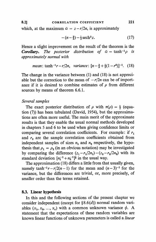
8.21 CORRELATION COEFFICIENT 221
which, at the maximum w = z - r/2n, is approximately
- (n - 2) - 2 sech2z. (17)
Hence a slight improvement on the result of the theorem is theCorollary. The posterior distribution of W = tanh-1p isapproximately normal with
mean : tanh-1 r - r/2n, variance : [n - z + 1(1- r2) ]-1. (18)
The change in the variance between (1) and (18) is not appreci-able but the correction to the mean of - r/2n can be of import-ance if it is desired to combine estimates of p from differentsources by means of theorem 6.6.1.
Several samplesThe exact posterior distribution of p with 7r(p) _ (equa-
tion (7)) has been tabulated (David, 1954), but the approxima-tions are often more useful. The main merit of the approximateresults is that they enable the usual normal methods developedin chapters 5 and 6 to be used when giving confidence limits orcomparing several correlation coefficients. For example: if r,and r2 are the sample correlation coefficients obtained fromindependent samples of sizes n1 and n2 respectively, the hypo-thesis that p, = P2 (in an obvious notation) may be investigatedby comparing the difference (z, - rl/2n,) - (z2 - r2/2n2) with itsstandard deviation [ni 1+n2']I in the usual way.
The approximation (18) differs a little from that usually given,namely tanh-1 r - r/2(n - 1) for the mean and (n - 3)-1 for thevariance, but the differences are trivial, or, more precisely, ofsmaller order than the terms retained.
8.3. Linear hypothesisIn this and the following sections of the present chapter we
consider independent (except for § 8.6 (d)) normal random vari-ables (x,, x2, ..., xn) with a common unknown variance 0. Astatement that the expectations of these random variables areknown linear functions of unknown parameters is called a linear
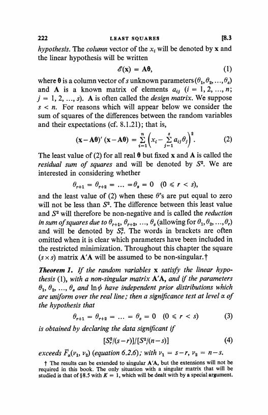
222 LEAST SQUARES [8.3
hypothesis. The column vector of the xi will be denoted by x andthe linear hypothesis will be written
6'(x) = AO, (1)
where 0 is a column vector of s unknown parameters (0k, 02i ..., B8)and A is a known matrix of elements a 5 (i = 1, 2, ..., n;j = 1, 2, ..., s). A is often called the design matrix. We supposes < n. For reasons which will appear below we consider thesum of squares of the differences between the random variablesand their expectations (cf. 8.1.21); that is,
n(x - AA)' (x - A8) _ (xj a af 6f2(2)
1
The least value of (2) for all real 9 but fixed x and A is called theresidual sum of squares and will be denoted by S2. We areinterested in considering whether
01+1=0r+2= =08=0 (0<r<s),and the least value of (2) when these 6's are put equal to zerowill not be less than S2. The difference between this least valueand S2 will therefore be non-negative and is called the reductionin sum of squares due to Br+x, Br+2, 08 (allowing for 01i 02, ..., 0r)
and will be denoted by S. The words in brackets are oftenomitted when it is clear which parameters have been included inthe restricted minimization. Throughout this chapter the square(s x s) matrix A'A will be assumed to be non-singular. t
Theorem 1. If the random variables x satisfy the linear hypo-thesis (1), with a non-singular matrix A'A, and if the parameters01i 02, ..., 08 and In c have independent prior distributions whichare uniform over the real line; then a significance test at level a ofthe hypothesis that
01+1=er+2=... =08=0 (0<r<s) (3)
is obtained by declaring the data significant if[S, 21(S - r)]/ [S2/(n - s)] (4)
exceeds F,,(v1, v2) (equation 6.2.6); with v1 = s - r, v2 = n - s.t The results can be extended to singular A'A, but the extensions will not be
required in this book. The only situation with a singular matrix that will bestudied is that of §8.5 with K = 1, which will be dealt with by a special argument.
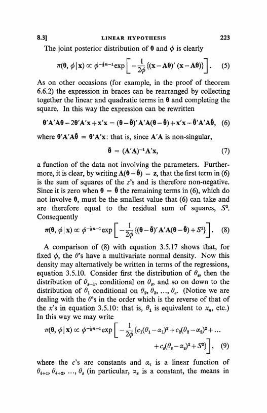
8.3] LINEAR HYPOTHESIS
The joint posterior distribution of 0 and is clearly
223
ir(e, c x) a 0-In-1 exp [ - 20 {(x - A9)' (x - A9)}] . (5)
As on other occasions (for example, in the proof of theorem6.6.2) the expression in braces can be rearranged by collectingtogether the linear and quadratic terms in 0 and completing thesquare. In this way the expression can be rewritten
9'A'A9 - 20'A'x + x'x = (9 - 9)' A'A(9 - 9) + x'x 9'A'A9, (6)
where 6'A'A9 = O'A'x: that is, since A'A is non-singular,
9 = (A'A)-IA'x, (7)
a function of the data not involving the parameters. Further-more, it is clear, by writing A(9 - 0) = z, that the first term in (6)is the sum of squares of the z's and is therefore non-negative.Since it is zero when 0 = 8 the remaining terms in (6), which donot involve 0, must be the smallest value that (6) can take andare therefore equal to the residual sum of squares, S2.Consequently
70, 0 I x) a: 0-In-1exp [_{(o_O)'A'A(o_O)+s2}]. (8)
A comparison of (8) with equation 3.5.17 shows that, forfixed ¢, the 0's have a multivariate normal density. Now thisdensity may alternatively be written in terms of the regressions,equation 3.5.10. Consider first the distribution of 08, then thedistribution of Bg-I, conditional on 08, and so on down to thedistribution of 01 conditional on 02, 03i ..., 0$. (Notice we aredealing with the 0's in the order which is the reverse of that ofthe x's in equation 3.5.10: that is, 0I is equivalent to x,,, etc.)In this way we may write
i(e, c I x) c 0-,In-1 exp [ - 20 {c1(0 - c 1)2 + c2(02 - a2)2 + ...
+ C8(03 - as)2 + S2}] , (9)
where the c's are constants and ai is a linear function ofei+1, Bi+21 .. 08 (in particular, a8 is a constant, the means in
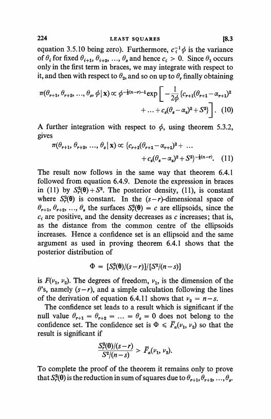
224 LEAST SQUARES [8.3
equation 3.5.10 being zero). Furthermore, c;' O is the varianceof Oi for fixed Oi+1, 0i+2, ..., 0$ and hence ci > 0. Since 01 occursonly in the first term in braces, we may integrate with respect toit, and then with respect to 02, and so on up to 0r finally obtaining
ir(0r+1, 0r+2, ..., 0s, c I x) a 0-1(n-r)-1 exp C - 20 {Cr+1(er+1- 0-"+]L),
+... +C8(08-as)2+S2}] . (10)
A further integration with respect to 0, using theorem 5.3.2,gives
)l2(Br+1, er+2, , O$ X) CC ff 1Cr+1(er+1- ar+L +
+ C8(08 - a8)2 + ,S'2}-1(n-r). (11)
The result now follows in the same way that theorem 6.4.1followed from equation 6.4.9. Denote the expression in bracesin (11) by S;(6)+S2. The posterior density, (11), is constantwhere Sr(6) is constant. In the (s-r)-dimensional space of01-+1, 0r+2, , 08 the surfaces Sr(6) = c are ellipsoids, since theci are positive, and the density decreases as c increases; that is,as the distance from the common centre of the ellipsoidsincreases. Hence a confidence set is an ellipsoid and the sameargument as used in proving theorem 6.4.1 shows that theposterior distribution of
_ [S2.(6)I(s-r)]I [S2/(n-s)]
is F(v1, v2). The degrees of freedom, v1, is the dimension of the0's, namely (s - r), and a simple calculation following the linesof the derivation of equation 6.4.11 shows that v2 = n - s.
The confidence set leads to a result which is significant if thenull value Or+1 = 0r+2 = ... = 08 = 0 does not belong to theconfidence set. The confidence set is < F8(v1i v2) so that theresult is significant if
S,(0)/(s - r)> Fa(v1, v2)S2/(n - s)
To complete the proof of the theorem it remains only to provethat S,1(0) is the reduction in sum of squares due to 0r+1, 0r+2, , 0s
8.3] LINEAR HYPOTHESIS 225
This is easily done by returning to the sum of squares, (2), inthe form of the expression in braces in (9). When
01+1 =Or+2 =... =0a -0
this is c1(01- z')2 + ... + c'(0 - a,')2 + Sr (O) + S2,
where ai is the value of ai when Br+1 = Br+2 = ... = 0" = 0(i 5 r). Since the c's are positive this has a minimum, whenei = ai (i r), of Sr(0) + S2. The equations 0i = as (i 5 r) arelinear equations in 01, 02, ..., 0r and will always have a solution.Hence SS(0) is the reduction, as required, and the theorem isproved.Corollary 1. The posterior distribution of S2/0 is x2 with(n - s) degrees of freedom.
This follows from (9) on integrating with respect to all the 0's.We obtain
n(o I X) CC0-+11n-sl-lexp [ - S2/20]
A comparison with equation 5.3.2 establishes the result.Corollary 2. The posterior distribution of a linear function,
8
gi 0i, of the parameters is such thati=1
g'(e - 0)/ [S2g'Cg/(n - s)]l (12)
has a t-distribution with v = n - s degrees of freedom; where g'is the row vector (g1, g2, ..., g8) and C is the matrix (A'A)-1.
For fixed 0, the 0's are multivariate normal, equation (8),with means 0 and dispersion matrix (A'A)-10, so that
S
g'e=F+gieii=1
is normal (a generalization to s variables of theorem 3.5.5) withmean g'0 and variance Og'Cg (theorem 3.3.2). Hence, bycorollary 1,
'T(Egi01, cilx)
oc c-*cn-8>-1 exp [ - S2/20]c-4
exp [ - .{g'(e - 0)}2/0gFCg]
The usual integration with respect to 0 (cf. equation 5.4.5)establishes the result.
The quantities 8i (equation (7)) are called the least squaresestimates of the 0i. They are the means of the posterior distribu-
15 L S II
226 LEAST SQUARES 18.3
tion of the 0's. Similarly, g'6 is the least squares estimate of g'9.The equations (A'A) 9 = A'x, whose solution is (7), are calledthe least squares equations. It is often useful to find the varianceof linear functions, g'9, of the 0i.
_q2(g'e _q2(g'CA'x 16, c)
= g'CA'ACgo,
since the x's are independent with common variance (corollaryto theorem 3.3.2). Finally, since C = (A'A)-1,
_q2(g'e 18, 0) = g'Cgc. (13)
This provides a means of calculating the denominator in (12).Corollary 3. Under the same conditions as in theorem 1 asignificance test at level a of the hypothesis that
bi;8; = 0 (i = r+1, r+2, ..., s), (14)=1
where B, a (s - r) x s matrix with elements b15, has rank (s - r), isobtained by declaring the data significant if
[Tr/(s-r)]I [S2/(n-s)] (15)
exceeds Fa(vl, v2) with v1 = s - r, v2 = n - s. Here T' is thereduction in sum of squares due to
8
bi;9; (i = r+1, r+2, ..., s);J=1
that is, Tr + S2 is the minimum of (2) when (14) obtains.Since B has full rank we can find a non-singular s x s matrix
Bo whose last (s - r) rows agree with the rows of B. Denote theelements of Bo by bit, i now running from 1 to s. Now changethe parameters to cP = Bo 8. Then J'(x) = A9 = AB', whichis a linear hypothesis in the i;f's, and the hypothesis to be tested,(14), is ?+11r+1 = 1'r+2 = ... _ Vs = 0. The result follows fromthe theorem.
Linear hypothesisThe theorem is one of the most important single results in
statistics. We have met several special cases before and had we
8.31 LINEAR HYPOTHESIS 227
stated it earlier could have deduced them from it. However, wepreferred to treat simple situations before passing to the generalcase. The linear hypothesis means that the random variablesbeing observed are, apart from independent random variationof variance ¢, known linear functions of unknown quantities.Since so many situations have a linear structure, or approxi-mately so, we should expect to find the result widely applicable.In its general form, (14), the hypothesis to be tested is alsolinear. The test is carried out by minimizing the sum of squares,first allowing the parameters to range freely, obtaining the mini-mum S2, and then restricting them according to the hypothesis,obtaining the minimum S2 + S,1 (or S2 + T, in the general case incorollary 3). It is important to observe, a point we will enlargeon below, that it is not necessary to consider the structure of Aor C = (A'A)-1: only the minima are required. Let us first seehow cases already considered fit into the linear hypothesisconcept.
Examples:(i) Normal means. Take s = 2 and write n = n1 + n2. Let
A be a matrix whose first column is n1 l's followed by n2 0'sand whose second column is n1 0's followed by n2 l's. That is,
,ff(xi) = 01 (1 5 i < nl), 'ff(xi) = 02 (n1 < i S n), (16)
and we have two independent samples of sizes n1 and n2 fromN(01, 0) and N(02, 0) respectively. Consider a test of the hypo-thesis that 0, = 02, that the means are equal (theorem 6.1.3).The sum of squares, (2), is
n, n(Xi - 01)2 + E (Xi - 02)2,
i=1 i=n1+1
with unrestricted minimum, equal to the residual, ofn, n lS 2 = (Xi -x1)2 + (Xi -x2)2,
i=1 i=n1+1
where xl, x2 are the means of the two samples. If 01 = 02 wehave to minimize with respect to the common value 0
n(Xi - 0)2,
i=115-2
228 LEAST SQUARES
nwith the result (xi - x)2,
i=1
[8.3
where x is the mean of the combined sample of n observations.It is easy to verify that the difference between these two minima is
(x1- x2)2 (ni 1 + n2 1)-1. (17)
Hence (with s = 2, r = 1), the F-statistic, (15), is
(xl - x2)2 (ni-1 +n2-')'/ [S2/(n -2)], (18)
with 1 and (n - 2) degrees of freedom. This is the same as thesignificance test derived from equation 6.1.6: the relationshipbetween the two equations is easily established by putting ,6 = 0,s2 = S2/(n - 2) in equation 6.1.6 and remembering that F = t2when the value of v1 = 1 (§ 6.2). Furthermore, the presentcorollary 1 is equivalent in this special case to theorem 6.1.2 andcorollary 2, with g'9 =01-02, to theorem 6.1.3. We leave it tothe reader to verify that theorem 6.4.1, for testing the differencebetween several normal means, is also a special case of thepresent theorem 1: indeed, we have used the method of proof ofthe earlier theorem to prove the new one.
(ii) Weighing. Another special case is the weighing exampleof §3.3. In §6.6, equations (12) and (13), the situation wasexpressed as a linear hypothesis with design matrix given inthe latter equation. However, there 0 was supposed known,equal to o.2. If 0 is unknown, since n = s = 4, there are nodegrees of freedom for error (n - s = 0) and no inferences arepossible. But if the whole experiment were repeated, so thatn = 8, still with s = 4, then the results of this section could beapplied. Corollary 1 gives the posterior distribution of theprecision (§ 5.1) and corollary 2 gives the posterior distribution ofany weight or of any difference of weights. Corollary 3 could beused, for example, to test the hypothesis that all the weights wereequal (01 = 02 = 03 = 04).
(iii) Linear regression. As a final special case consider linearhomoscedastic normal regression and the results obtained in§ 8.1. Replace the x's of the present section by y's and (01, 02)by (a, /3). Then if the ith row of A is
(1, xi-x), (19)
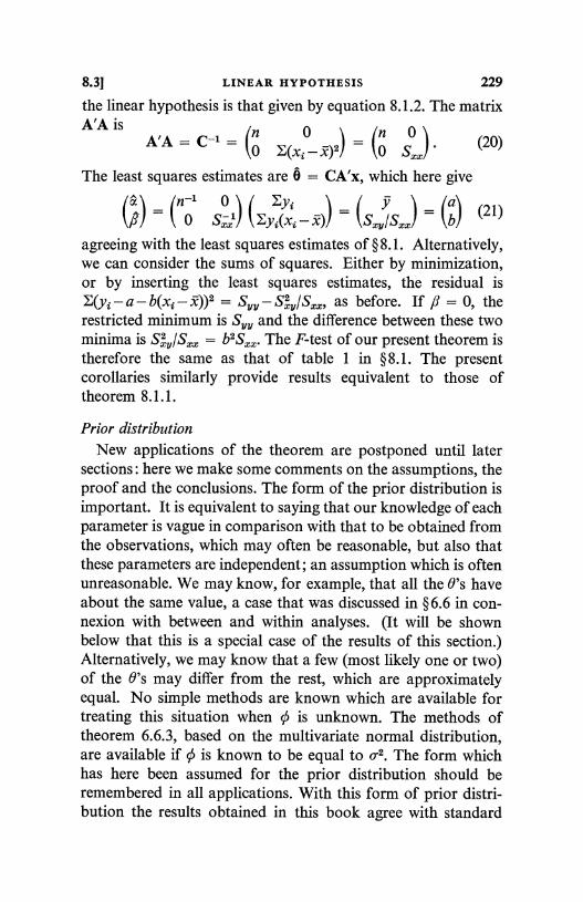
8.31 LINEAR HYPOTHESIS 229
the linear hypothesis is that given by equation 8.1.2. The matrixA'A is n 0 In 0
A'A = 1= (0 E(xi-x)2) _ (0 S..). (20)
The least squares estimates are 9 = CA'x, which here give
(n01 S. Y-Y (xz - x)) - S/S.:.) - `b) (21)
agreeing with the least squares estimates of §8. 1. Alternatively,we can consider the sums of squares. Either by minimization,or by inserting the least squares estimates, the residual isE(y;, - a - b(xi - x))2 = Sy, - Sxy/S, as before. If /3 = 0, therestricted minimum is Spy and the difference between these twominima is S2,/ S.,., = b2S,,x. The F-test of our present theorem istherefore the same as that of table 1 in §8.1. The presentcorollaries similarly provide results equivalent to those oftheorem 8.1.1.
Prior distributionNew applications of the theorem are postponed until later
sections : here we make some comments on the assumptions, theproof and the conclusions. The form of the prior distribution isimportant. It is equivalent to saying that our knowledge of eachparameter is vague in comparison with that to be obtained fromthe observations, which may often be reasonable, but also thatthese parameters are independent; an assumption which is oftenunreasonable. We may know, for example, that all the 0's haveabout the same value, a case that was discussed in § 6.6 in con-nexion with between and within analyses. (It will be shownbelow that this is a special case of the results of this section.)Alternatively, we may know that a few (most likely one or two)of the 6's may differ from the rest, which are approximatelyequal. No simple methods are known which are available fortreating this situation when 0 is unknown. The methods oftheorem 6.6.3, based on the multivariate normal distribution,are available if 0 is known to be equal to Q2. The form whichhas here been assumed for the prior distribution should beremembered in all applications. With this form of prior distri-bution the results obtained in this book agree with standard
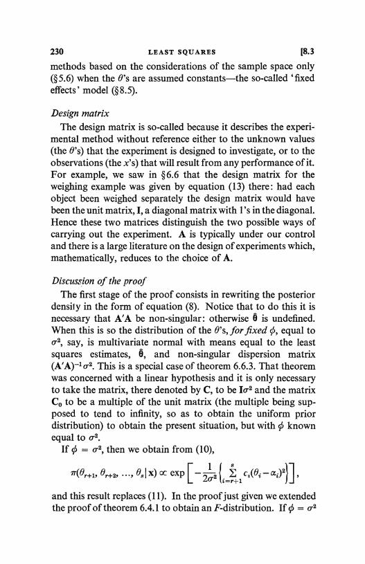
230 LEAST SQUARES [8.3
methods based on the considerations of the sample space only(§5.6) when the 0's are assumed constants-the so-called `fixedeffects' model (§8.5).
Design matrixThe design matrix is so-called because it describes the experi-
mental method without reference either to the unknown values(the 0's) that the experiment is designed to investigate, or to theobservations (the x's) that will result from any performance of it.For example, we saw in § 6.6 that the design matrix for theweighing example was given by equation (13) there: had eachobject been weighed separately the design matrix would havebeen the unit matrix, I, a diagonal matrix with l's in the diagonal.Hence these two matrices distinguish the two possible ways ofcarrying out the experiment. A is typically under our controland there is a large literature on the design of experiments which,mathematically, reduces to the choice of A.
Discussion of the proofThe first stage of the proof consists in rewriting the posterior
density in the form of equation (8). Notice that to do this it isnecessary that A'A be non-singular: otherwise 6 is undefined.When this is so the distribution of the 0's, for fixed 0, equal tov2, say, is multivariate normal with means equal to the leastsquares estimates, 6, and non-singular dispersion matrix(A'A)-1 0-2. This is a special case of theorem 6.6.3. That theoremwas concerned with a linear hypothesis and it is only necessaryto take the matrix, there denoted by C, to be 10-2 and the matrixCo to be a multiple of the unit matrix (the multiple being sup-posed to tend to infinity, so as to obtain the uniform priordistribution) to obtain the present situation, but with 0 knownequal to .2.
If 0 = v2, then we obtain from (10),
1
i
s (
1T(er+1, 0r+2, - .., 08 I x) ac exP - 2 c (01- CGi)2 I
ZQ =r+1
and this result replaces (11). In the proof just given we extendedthe proof of theorem 6.4.1 to obtain an F-distribution. If 0 = 0-2
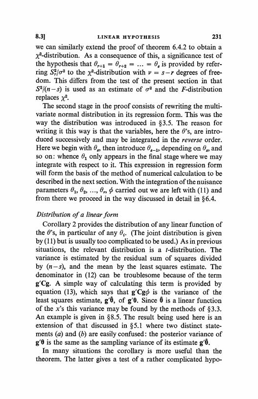
8.3] LINEAR HYPOTHESIS 231
we can similarly extend the proof of theorem 6.4.2 to obtain aX2-distribution. As a consequence of this, a significance test ofthe hypothesis that Br+1 = Br+2 = ... = B$ is provided by refer-ring S;/v-2 to the X2-distribution with v = s - r degrees of free-dom. This differs from the test of the present section in thatS2/(n - s) is used as an estimate of o.2 and the F-distributionreplaces xs
The second stage in the proof consists of rewriting the multi-variate normal distribution in its regression form. This was theway the distribution was introduced in §3.5. The reason forwriting it this way is that the variables, here the B's, are intro-duced successively and may be integrated in the reverse order.Here we begin with 83, then introduce 08_1, depending on 08, andso on: whence 81 only appears in the final stage where we mayintegrate with respect to it. This expression in regression formwill form the basis of the method of numerical calculation to bedescribed in the next section. With the integration of the nuisanceparameters 01i 02, ..., Br, 0 carried out we are left with (11) andfrom there we proceed in the way discussed in detail in §6.4.
Distribution of a linear formCorollary 2 provides the distribution of any linear function of
the B's, in particular of any 01. (The joint distribution is givenby (11) but is usually too complicated to be used.) As in previoussituations, the relevant distribution is a t-distribution. Thevariance is estimated by the residual sum of squares dividedby (n - s), and the mean by the least squares estimate. Thedenominator in (12) can be troublesome because of the termg'Cg. A simple way of calculating this term is provided byequation (13), which says that g'Cgc is the variance of theleast squares estimate, g'9, of g'9. Since 9 is a linear functionof the x's this variance may be found by the methods of § 3.3.An example is given in §8.5. The result being used here is anextension of that discussed in §5.1 where two distinct state-ments (a) and (b) are easily confused: the posterior variance ofg'9 is the same as the sampling variance of its estimate g'6.
In many situations the corollary is more useful than thetheorem. The latter gives a test of a rather complicated hypo-
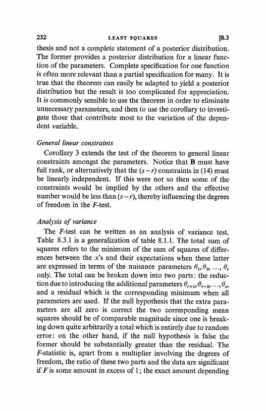
232 LEAST SQUARES [8.3
thesis and not a complete statement of a posterior distribution.The former provides a posterior distribution for a linear func-tion of the parameters. Complete specification for one functionis often more relevant than a partial specification for many. It istrue that the theorem can easily be adapted to yield a posteriordistribution but the result is too complicated for appreciation.It is commonly sensible to use the theorem in order to eliminateunnecessary parameters, and then to use the corollary to investi-gate those that contribute most to the variation of the depen-dent variable.
General linear constraintsCorollary 3 extends the test of the theorem to general linear
constraints amongst the parameters. Notice that B must havefull rank, or alternatively that the (s - r) constraints in (14) mustbe linearly independent. If this were not so then some of theconstraints would be implied by the others and the effectivenumber would be less than (s - r), thereby influencing the degreesof freedom in the F-test.
Analysis of variance
The F-test can be written as an analysis of variance test.Table 8.3.1 is a generalization of table 8.1.1. The total sum ofsquares refers to the minimum of the sum of squares of differ-ences between the x's and their expectations when these latterare expressed in terms of the nuisance parameters 01,02, ..., eronly. The total can be broken down into two parts : the reduc-tion due to introducing the additional parameters er+1, er+29 , eseand a residual which is the corresponding minimum when allparameters are used. If the null hypothesis that the extra para-meters are all zero is correct the two corresponding meansquares should be of comparable magnitude since one is break-ing down quite arbitrarily a total which is entirely due to randomerror: on the other hand, if the null hypothesis is false theformer should be substantially greater than the residual. TheF-statistic is, apart from a multiplier involving the degrees offreedom, the ratio of these two parts and the data are significantif F is some amount in excess of 1; the exact amount depending
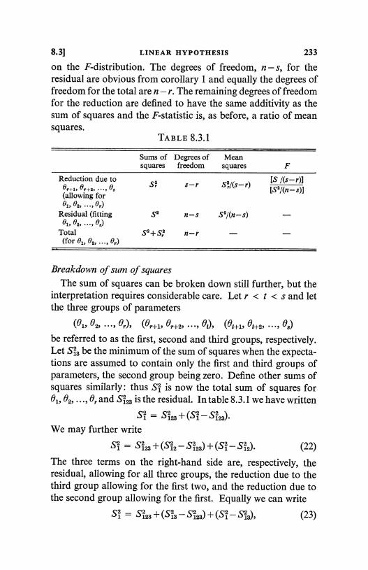
8.31 LINEAR HYPOTHESIS 233
on the F-distribution. The degrees of freedom, n - s, for theresidual are obvious from corollary 1 and equally the degrees offreedom for the total are n - r. The remaining degrees of freedomfor the reduction are defined to have the same additivity as thesum of squares and the F-statistic is, as before, a ratio of meansquares.
TABLE 8.3.1
Sums ofsquares
Degrees offreedom
Meansquares F
Reduction due to IS /(s-r)1Br+1, Br+2, , 01
Sr s-r S2,/(s-r)[S2l(n-s)]
(allowing for01, B21 ..., Br)
Residual (fitting S2 n-s S'/(n-s)01, 02, ..., es)
Total(for 01, 02, ..., er)
S2+S; n-r
Breakdown of sum of squares
The sum of squares can be broken down still further, but theinterpretation requires considerable care. Let r < t < s and letthe three groups of parameters
(01, 02, ..., °r), (0r+1, Br+29 ..., Bt), (0+1, 0t+2, ..., 08)
be referred to as the first, second and third groups, respectively.Let S13 be the minimum of the sum of squares when the expecta-tions are assumed to contain only the first and third groups ofparameters, the second group being zero. Define other sums ofsquares similarly: thus S2 is now the total sum of squares for81, 02i ...,Brand S123 is the residual. In table 8.3.1 we have written
S1 = S2 +(S1 - s123We may further write
2S1 - "5123 + Cs12 - 512 23 +(S21- 512 (22)
The three terms on the right-hand side are, respectively, theresidual, allowing for all three groups, the reduction due to thethird group allowing for the first two, and the reduction due tothe second group allowing(S23for the first. /Equally we can write
S2- "5123 + 1-5123 + ls1-513 , (23)
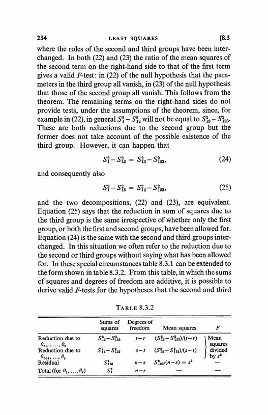
234 LEAST SQUARES [8.3
where the roles of the second and third groups have been inter-changed. In both (22) and (23) the ratio of the mean squares ofthe second term on the right-hand side to that of the first termgives a valid F-test: in (22) of the null hypothesis that the para-meters in the third group all vanish, in (23) of the null hypothesisthat those of the second group all vanish. This follows from thetheorem. The remaining terms on the right-hand sides do notprovide tests, under the assumptions of the theorem, since, forexample in (22), in general S1- S12 will not be equal to SS3 - S2123.These are both reductions due to the second group but theformer does not take account of the possible existence of thethird group. However, it can happen that
sl-s 1.2 - S13-512 3,
and consequently also
S2 (25)
and the two decompositions, (22) and (23), are equivalent.Equation (25) says that the reduction in sum of squares due tothe third group is the same irrespective of whether only the firstgroup, or both the first and second groups, have been allowed for.Equation (24) is the same with the second and third groups inter-changed. In this situation we often refer to the reduction due tothe second or third groups without saying what has been allowedfor. In these special circumstances table 8.3.1 can be extended tothe form shown in table 8.3.2. From this table, in which the sumsof squares and degrees of freedom are additive, it is possible toderive valid F-tests for the hypotheses that the second and third
TABLE 8.3.2
Sums of Degrees ofsquares freedom Mean squares F
Reduction due to Sia-Si33 t-r (S1a-S138)/(t-r) Mean01+1, ..., Bt squares
Reduction due to S12-Si33 s-t (Sia-Siza)l(s-t) dividedBt+1r ..., B3 by s3
Residual S2133 n-s S2133/(n-s) = s3 -Total (for 0 , ..., B,) S1 n-r - -
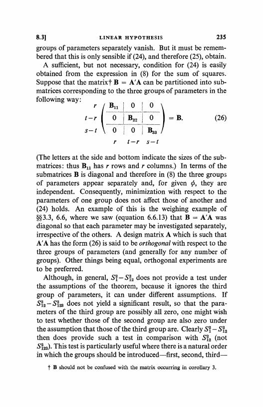
8.31 LINEAR HYPOTHESIS 235
groups of parameters separately vanish. But it must be remem-bered that this is only sensible if (24), and therefore (25), obtain.
A sufficient, but not necessary, condition for (24) is easilyobtained from the expression in (8) for the sum of squares.Suppose that the matrix' B = A'A can be partitioned into sub-matrices corresponding to the three groups of parameters in thefollowing way:
t-r--------------------------------------
0 B22 0 = B. (26)
S - t 0 0 B33
r t-r s-t(The letters at the side and bottom indicate the sizes of the sub-matrices: thus B11 has r rows and r columns.) In terms of thesubmatrices B is diagonal and therefore in (8) the three groupsof parameters appear separately and, for given 0, they areindependent. Consequently, minimization with respect to theparameters of one group does not affect those of another and(24) holds. An example of this is the weighing example of§§3.3, 6.6, where we saw (equation 6.6.13) that B = A'A wasdiagonal so that each parameter may be investigated separately,irrespective of the others. A design matrix A which is such thatA'A has the form (26) is said to be orthogonal with respect to thethree groups of parameters (and generally for any number ofgroups). Other things being equal, orthogonal experiments areto be preferred.
Although, in general, S1- S12 does not provide a test underthe assumptions of the theorem, because it ignores the thirdgroup of parameters, it can under different assumptions. IfS2 _S2
23 does not yield a significant result, so that the para-meters of the third group are possibly all zero, one might wishto test whether those of the second group are also zero underthe assumption that those of the third group are. Clearly S 2 - S21 12
then does provide such a test in comparison with S12 (not"5123). This test is particularly useful where there is a natural orderin which the groups should be introduced-first, second, third-
t B should not be confused with the matrix occurring in corollary 3.
236 LEAST SQUARES [8.3
and examples will be found in §§ 8.6 (a) and (c). Compare, also,this argument with that suggested in § 6.3 for deciding whetherto use Behrens's test or a t-test.
Least squares estimatesIt follows from (8) that the statistics 8 and S2 are jointly
sufficient for 0 and 0. The least square estimates and the residualare therefore important quantities to calculate in any analysis ofa linear hypothesis. The calculation can be done in two ways:by finding (A'A)-1 = C and hence 6 from (7), and then
S2 = x'x - O'A'AO, from (6), (27)
= x'x - x'ACA'x, from (7) (28)
(from which it appears that x'x and A'x are also jointly suffi-cient); or alternatively by actual minimization of the sum ofsquares, the minimum being S2, the values of 0 at the minimumbeing O. The former method is to be preferred in the case ofa general A and we discuss it in the next section: the calculationdepending on the inversion of A'A. The latter method is moreconvenient when the structure of A is particularly simple, as itoften is in well-designed (for example, orthogonal) experiments.Examples are given in §§8.5, 8.6.
8.4. Computational methodsIn this section we consider how the computations necessary to
perform the tests of the previous section may be arranged whenthe matrix A'A is general and it is therefore not possible to takeadvantage of any special structure that it might have. Themethods are designed for use with desk calculating machines.
If f' and g' are two row-vectors, or simply rows,
f' = (Al f2, ..., fn), g' - (g1, g2, ..., gn),
each of n elements; then by the product of these two rows weIt
mean the scalar product I figi. The product of a row andi=1
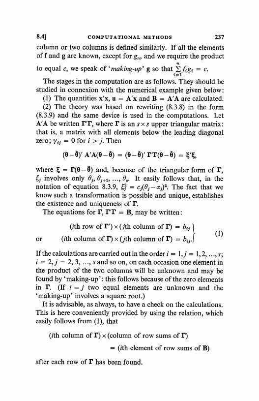
8.41 COMPUTATIONAL METHODS 237
column or two columns is defined similarly. If all the elementsoff and g are known, except for g,,, and we require the product
nto equal c, we speak of 'making-up' g so that E figi = c.
i=1
The stages in the computation are as follows. They should bestudied in connexion with the numerical example given below :
(1) The quantities x'x, u = A'x and B = A'A are calculated.(2) The theory was based on rewriting (8.3.8) in the form
(8.3.9) and the same device is used in the computations. LetA'A be written r'r, where r is an s x s upper triangular matrix:that is, a matrix with all elements below the leading diagonalzero; yij = 0 for i > j. Then
(e-0)' A'A(9-0) = (e-0)'r'r(s-e)
where = r(e - 0) and, because of the triangular form of r,6; involves only ej, ej+1, ..., O. It easily follows that, in thenotation of equation 8.3.9, 6; = c5(01- aj)2. The fact that weknow such a transformation is possible and unique, establishesthe existence and uniqueness of r.
The equations for r, r'r = B, may be written:
(ith row of r) x (jth column of r) = bi3
or (ith column of r) x (jth column of r) = bi;.(1)
If the calculations are carried out in the order i = 1, j = 1, 2, ..., s;i = 2, j = 2, 3, ..., s and so on, on each occasion one element inthe product of the two columns will be unknown and may befound by 'making-up': this follows because of the zero elementsin r. (If i = j two equal elements are unknown and the'making-up' involves a square root.)
It is advisable, as always, to have a check on the calculations.This is here conveniently provided by using the relation, whicheasily follows from (1), that
(ith column of r) x (column of row sums of r)
= (ith element of row sums of B)
after each row of r has been found.
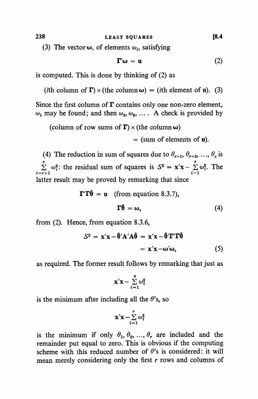
238 LEAST SQUARES
(3) The vector w, of elements wi, satisfying
[8.4
r'w = u (2)
is computed. This is done by thinking of (2) as
(ith column of r) x (the column w) = (ith element of u). (3)
Since the first column of r contains only one non-zero element,wl may be found; and then w2, W3, .... A check is provided by
(column of row sums of r) x (the column w)
= (sum of elements of u).
(4) The reduction in sum of squares due to Br+1, 0r+2, ..., 63 isS 8
(,l: the residual sum of squares is S2 = x'x - c4 Thei=r+1 i=1
latter result may be proved by remarking that since
r'r6 = u (from equation 8.3.7),
rb = w,
from (2). Hence, from equation 8.3.6,
S2 = x'x-O'A'AO = x'x-O'r'rO
= X'x -W'W'
(4)
(5)
as required. The former result follows by remarking that just as
x'x - wit=1
is the minimum after including all the B's, so
rx'x - EOJ%
i=1
is the minimum if only 01, 02, ..., 6, are included and theremainder put equal to zero. This is obvious if the computingscheme with this reduced number of B's is considered: it willmean merely considering only the first r rows and columns of
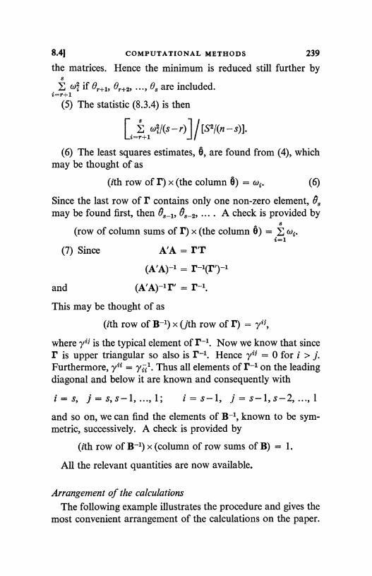
8.4] COMPUTATIONAL METHODS 239
the matrices. Hence the minimum is reduced still further by8
(01 if 0r+1, 0r+2, . . 03 are included.i=r+1
(5) The statistic (8.3.4) is
ir+1&)i /(s -r)J / ['S2/(n - s) J.[
(6) The least squares estimates, 8, are found from (4), whichmay be thought of as
(ith row of r) x (the column 9) = Wi (6)
Since the last row of r contains only one non-zero element, O,may be found first, then A check is provided by
(row of column sums of r) x (the column 9) = E Wi.i=1
(7) Since A'A = F'F(A'A)-1 = F-1(F')-1
and (A'A)-1F' = F-1.
This may be thought of as
(ith row of B-1) x (jth row of r) = yif,
where yit is the typical element of F. Now we know that sinceF is upper triangular so also is r-1. Hence yip = 0 for i > j.Furthermore, yii = y221. Thus all elements of r-1 on the leadingdiagonal and below it are known and consequently with
i=s, j=s,s-1,...,1; i=s-1, j=s-l,s-2,...,1and so on, we can find the elements of B-1, known to be sym-metric, successively. A check is provided by
(ith row of B-1) x (column of row sums of B) = 1.
All the relevant quantities are now available.
Arrangement of the calculationsThe following example illustrates the procedure and gives the
most convenient arrangement of the calculations on the paper.
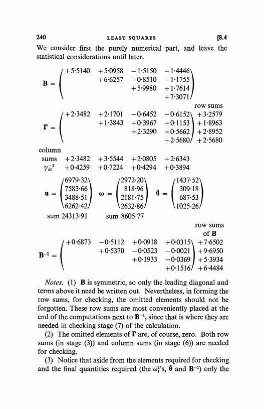
240 LEAST SQUARES [8.4
We consider first the purely numerical part, and leave thestatistical considerations until later.
+5-5140 +5-0958 -1.5150 -1.4446
B= +6-6257 -0-8510 -1.1755+5-9980 +1-7614
+7-3071row sums
+2-3482 +2-1701 -0-6452 -0-6152 + 3.2579
r= +1-3843 +0.3967 +0.1153
)
+1-8963+2.3290 +0.5662 +2.8952
column+2-5680 +2-5680
sums +2-3482 +3-5544 +2-0805 +2-6343y221 +0.4259 +0.7224 +0.4294 +0.3894
6979.32 2972.20 1437.527583.66 818.96 309.18
°
=
3488.51_
2181.75_
687.536262.42 2632.86 1025.26
sum 24313.91 sum 9605.77
B-1 =
row sumsof B
+0.6873 -0.5112 +0.0918 +0.0315 +7.6502+0.5370 -0.0523 -0.0021 +9.6950
+0.1933 -0.0369 +5.3934+0.1516 +6.4484
Notes. (1) B is symmetric, so only the leading diagonal andterms above it need be written out. Nevertheless, in forming therow sums, for checking, the omitted elements should not beforgotten. These row sums are most conveniently placed at theend of the computations next to B-1, since that is where they areneeded in checking stage (7) of the calculation.
(2) The omitted elements of r are, of course, zero. Both rowsums (in stage (3)) and column sums (in stage (6)) are neededfor checking.
(3) Notice that aside from the elements required for checkingand the final quantities required (the WA's, 0 and B-1) only the
8.41 COMPUTATIONAL METHODS 241
matrix r, the vector u and the inverses y2il = yii have to berecorded. Since the main source of error with desk machineslies in the transfer from paper to machine and vice versa theopportunities for error are reduced by this procedure.
(4) All operations consist of row or column multiplicationswith'making-up'. The use of only one basic operation makes forsimplicity.
(5) Experience shows that this method is of high accuracy.It is usually enough to take one more significant figure in thecalculations than will be needed in the final answer to allow forrounding-off errors.
Multiple regressionThe case of general A most usually arises in a generalization
of the situation of § 8.1. Consider s variables (y, x1, x2, ..., X3-):y is a random variable whose distribution depends on the x's ina way to be described. The x's may be random or not; ifrandom, then they are ancillary (see the discussion in §8.1). Ifthe x's take values xil, xi2, ..., xi, 3-1 (i = 1, 2, ..., n) the randomvariable y, with value yi, is normally distributed with mean
3-1'ff(Y I xil, xi2, ..., xi, 3-1) = x + E fj(xi j - X. J) (7)
J=1
and _q2(yI xi1, xi2, ..., xi, 3-1) = T, (8)
nwhere, as usual, x. j = xij/n.
2=1
In these circumstances y is said to have a (linear homoscedastic)multiple regression on the x's. The words in brackets are usuallyomitted. If the yi are, for these values of the x's, independent,we have a random sample from the multiple regression. /.lj iscalled the multiple regression coefficient of y on xj. The notationfor it is an abbreviation since it also depends on the other vari-ables included in the regression and, in general, would change ifany of them were excluded or others introduced. The coefficientmeasures the change in the dependent variable caused by a unitchange in xj, the others being held constant.
16 LS 11
242 LEAST SQUARES 18.4
The situation is clearly a linear hypothesis: in the notationof §8.3:
and
A=
X' = (!"1, Y2, ..., Yn), (9)
e' = (a, A1, ..., RS-1) (10)
1 x11-x.1 x12-x.21 x21- x.1 X22-X.2
xnl-x.1 xn2-x.2
(compare the linear regression example in § 8.3 especially equa-tion 8.3.19). Typically the xi; cannot be conveniently chosen,because the x's are random or are otherwise not under control,and the design matrix has a general form, apart from the firstcolumn. The test of theorem 8.3.1 is a test that
A.=N,+1= ... =Ns-1=0:that is, a test of the hypothesis that the random variable y doesnot depend on the variables x x,+1, ..., x8_1.
The fact that the first column of A consists entirely of l's canbe exploited. We easily see that
n 0 0 ... 0
where
A'A = 0 b11 b12 ... b1,8_1
0 b1,8_1 b2,s-1 ... bs-1,8-1
x1,8-1- x.8-1
x2,s-1-x.s-1 (11)
n
bit = kkl(xki - x. i) (xkj - x.5),
(12)
(13)
the sum of squares (i = j) and products (i + j) of the x's abouttheir means. Because of the zeros in A'A; in equation 8.3.8 theterm in 01 (here Bl = a) is separate from the rest and we mayperform an integration with respect to it to obtain (in themultiple regression notation)
?r(F'1, Al ..., Ns-l, 01X)
a O-lc4-1>-1 exp [- {(P - R)'B(I3 - P) + S2}/20], (14)
which is the same form as before with B the matrix whosetypical element is bit, equation (13). It is also clear from
8.41 COMPUTATIONAL METHODS 243
equation 8.3.7 that ^a = y = yi/n, and hence, from equationi=1
8.3.6, that the residual sum of squares is
S2 = x'x - 6'A'A9 = Eyz - ny2- fi'B(3
= Z(Yi-Y)2-(3'B(3. (15)
Hence the form of (14) is the same as that of (8.3.8) withn reduced by one and the observed variables replaced by devia-tions from their means. We have the usual phenomenon that thepresence of an unknown mean reduces the degrees of freedomby 1. The calculations can be carried through with N1,N2, ..., fls-1only, and deviations from the means.
Numerical example
The numerical example concerned a situation of the multipleregression form, where a sample of thirty small farms ofsimilar character was studied over a period of three years. Thevariable y was income of a farm, and it was desired to see howthis was affected by x1, the size of the farm; x2, the standardizedproduction and by two indices, x3 and x4, of yield and feeding.
The matrix B of the numerical example gives the sums ofsquares and products, equation (13), of the x variables usuallycalled the independent variables. These have been given here insuitable units to make the four diagonal entries of B of the sameorder. Such changes of scale are desirable in order to simplifythe calculations. The vector u is the vector of sums of productsof y with the x's: namely the ith element is
n n /Ui
= I Yk// (xki - X. i) _ Z (Yk -Y) lxki - X. J.k=1 k=1
(16)
The total sum of squares of the y's is E(yi - y)2 = 40, 572, 526.Hence the residual sum of squares is this less
4
01 = 21, 196, 653,i=1
giving S2 = 19, 375, 873 on (29 - 4) = 25 degrees of freedom.As an example of the test of theorem 8.3.1 consider a test of
r6-2
244 LEAST SQUARES [8.4
whether /33 = Q4 = 0; that is, of whether the income dependson the two indices. This is provided by referring
[(&3 +(04)/2]/ [S2/25] (17)
to the F-distribution with 2 and 25 degrees of freedom. Thenumerical value of (17) is 7.54 and the upper 1 % value of F is5.57. The result is therefore significant at 1 %: or, in Bayesianterms, we are at least 99 % confident that the yield does dependon the indices. The significance level is greater than 0.1 %,however, since at that level the F value is 9.22.
A test of dependence on any one of the x's is provided bycorollary 2 of the last section. For example, a test of thedependence on x2, the standardized production, is obtained byreferring
309.18/[S2 x 0.5370/25]4 = 0.48
to the t-distribution with 25 degrees of freedom. (fl2 = 309.18and 0.5370 is the appropriate element in B-1 = C.) The 5value for t is 2.06 so that the result is not significant. There is,therefore, fair evidence to suggest that the income is not affectedby the standardized production, after allowance for the otherfactors.
Consequences of non-orthogonality
The only hypotheses that it is possible to test using the compu-tational lay-out suggested above are that
Rr+1=Qr+2=... =ft4=0 for r=0,1,2,3(by the theorem) or
/J=O for i = 1, 2, 3, 4
(by corollary 2). It is not immediately possible, for example,to test the hypothesis that /31 = N2 = 0. To do this it would benecessary to rearrange the matrix B and the vector u so that thelast two rows and columns referred to x1 and x2; when a testwould be obtained by using what would then be t3 + W4, corre-sponding to the last two parameters introduced. Before begin-ning the computations it is therefore important to considerwhich hypotheses are the most important to test and to order the
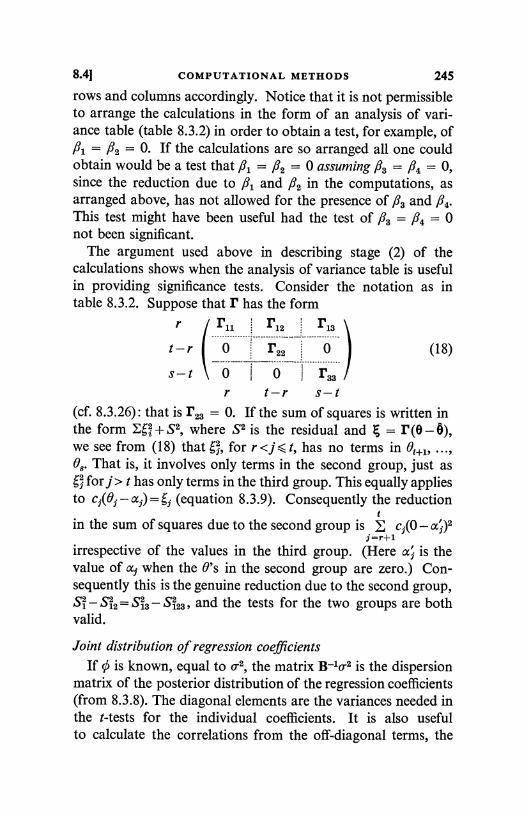
8.41 COMPUTATIONAL METHODS 245
rows and columns accordingly. Notice that it is not permissibleto arrange the calculations in the form of an analysis of vari-ance table (table 8.3.2) in order to obtain a test, for example, offl, = 62 = 0. If the calculations are so arranged all one couldobtain would be a test that ft1 = /32 = 0 assuming /33 = Q4 = 0,since the reduction due to /31 and 82 in the computations, asarranged above, has not allowed for the presence of fl,, and N4.This test might have been useful had the test of N3 = 64 = 0not been significant.
The argument used above in describing stage (2) of thecalculations shows when the analysis of variance table is usefulin providing significance tests. Consider the notation as intable 8.3.2. Suppose that r has the form
r r11 r12 r13............. ...........-
t-r 0 r22 0 (18)
S- t 0 0 i r33r t-r s-t
(cf. 8.3.26) : that is r23 = 0. If the sum of squares is written inthe form Egg + S2, where S2 is the residual and >; = r (9 - 0),we see from (18) that g;, for r <j 5 t, has no terms in 0j+1,08. That is, it involves only terms in the second group, just asi for j > t has only terms in the third group. This equally applies
to c,(05 - a) = 9 f (equation 8.3.9). Consequently the reductiont
in the sum of squares due to the second group is c,(0 - 4)27 =r+1
irrespective of the values in the third group. (Here a'; is thevalue of ac when the 0's in the second group are zero.) Con-sequently this is the genuine reduction due to the second group,S i - Sit = Sl3 - Sits, and the tests for the two groups are bothvalid.
Joint distribution of regression coefficientsIf 0 is known, equal to u2, the matrix B-10-2 is the dispersion
matrix of the posterior distribution of the regression coefficients(from 8.3.8). The diagonal elements are the variances needed inthe t-tests for the individual coefficients. It is also usefulto calculate the correlations from the off-diagonal terms, the
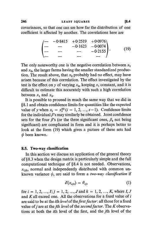
246 LEAST SQUARES [8.4
covariances, so that one can see how far the distribution of onecoefficient is affected by another. The correlations here are
- -08415 +0.2519 +0.0976- - 0.1623 -0-0074).- -0.2155 (19)
The only noteworthy one is the negative correlation between xland x2, the larger farms having the smaller standardized produc-tion. The result above, that x2 probably had no effect, may havearisen because of this correlation. The effect investigated by thetest is the effect on y of varying x2, keeping x, constant, and it isdifficult to estimate this accurately with such a high correlationbetween xl and x2.
It is possible to proceed in much the same way that we did in§8.1 and obtain confidence limits for quantities like the expectedvalue of y when xi = xz°) (i = 1, 2, ..., s-1). Confidence limitsfor the individual /3's may similarly be obtained. Joint confidencesets for the four /3's (or the three significant ones, N2 not beingsignificant) are complicated in form and it is perhaps better tolook at the form (19) which gives a picture of these sets had0 been known.
8.5. Two-way classificationIn this section we discuss an application of the general theory
of § 8.3 when the design matrix is particularly simple and the fullcomputational technique of § 8.4 is not needed. Observations,xijk, normal and independently distributed with common un-known variance 0, are said to form a two-way classification if
'e(x'iik) = ei3, (1)
for i = 1, 2, ..., I; j = 1, 2, ..., J and k = 1, 2, ..., K, where I, Jand K all exceed one. All the observations for a fixed value of iare said to be at the ith level of the first factor: all those for a fixedvalue of j are at the jth level of the second factor. The K observa-tions at both the ith level of the first, and the jth level of the
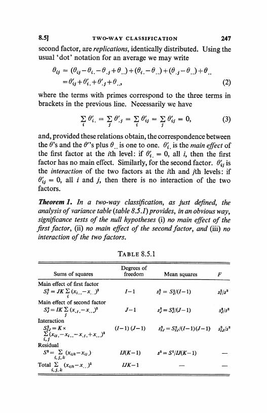
8.5] TWO-WAY CLASSIFICATION 247
second factor, are replications, identically distributed. Using theusual `dot' notation for an average we may write
Oil = (Oil -oi.-o.j+o.) +(0i.-o.) +(0,j-o.) +o..=0ij+8%.+o'j+o., (2)
where the terms with primes correspond to the three terms inbrackets in the previous line. Necessarily we have
(3)
and, provided these relations obtain, the correspondence betweenthe 0's and the 0"s plus 0._ is one to one. 0%. is the main effect ofthe first factor at the ith level: if 0i. = 0, all i, then the firstfactor has no main effect. Similarly, for the second factor. 0zj isthe interaction of the two factors at the ith and jth levels: if0 = 0, all i and j, then there is no interaction of the twofactors.
Theorem 1. In a two-way classification, as just defined, theanalysis of variance table (table 8.5. 1) provides, in an obvious way,significance tests of the null hypotheses (i) no main effect of thefirst factor, (ii) no main effect of the second factor, and (iii) nointeraction of the two factors.
TABLE 8.5.1
Sums of squaresDegrees offreedom Mean squares F
Main effect of first factorS. = JK I (x; )'-x I-1 4 = SI/(I-1) s1/s2.....i
Main effect of second factorS'r=IKE(x,f,-x,,)' J-1 s2 =S/(J-1) st/s'
InteractionSir=Kx (I-1) (J-1) S1J=S,2,rI(I-1)(J-1)
s127ls2E (xs.-xt..-X.,.+x...)'i, j
ResidualS' = E (x{7k - x0,) IJ(K-1) s' = S'/IJ(K-1)
i,j,kTotal E (xs;k-x,,)' IJK-1
i,5,k
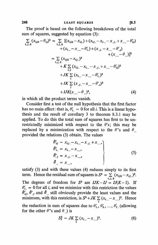
248 LEAST SQUARES [8.5
The proof is based on the following breakdown of the totalsum of squares, suggested by equation (3) :
: i (xiyk-ei;)2 = E [(xifk-xi3)+(xii.-xi..-x.1.+x...-0i3)i,.7,k i,1,k
+(x...0..)]2(xi;k-xii,)2
i,.7, k
+K (x1.-xi..-x,;,+x...Bii)2+JK (xi..-x...-0%.)2
+IK 2 (x.,.-x...-0:;)2
+IJK(x... - 0..)2, (4)
in which all the product terms vanish.Consider first a test of the null hypothesis that the first factor
has no main effect: that is, 0i, = 0 for all i. This is a linear hypo-thesis and the result of corollary 3 to theorem 8.3.1 may beapplied. To do this the total sum of squares has first to be un-restrictedly minimized with respect to the 0's; this may bereplaced by a minimization with respect to the 0"s and 0provided the relations (3) obtain. The values
0i; = xi;,-xi..-x.f.+x...'
(5)X. X...'
satisfy (3) and with these values (4) reduces simply to its firstterm. Hence the residual sum of squares is S2 = Z (xi;k - X;.)2.
i,f,kThe degrees of freedom for S2 are IJK-IJ = IJ(K-1). If0i. = 0 for all i, and we minimize with this restriction the values8z;, 0;; and 0 still obviously provide the least values and theminimum, with this restriction, is S2 +JK (xi.. - x..,)2. Hence
,, 02., ..., 01, (allowingthe reduction in sum of squares due to 01'for the other 0"s and is
Si = JKE (xi..-x...)2. (6)i
8.51 TWO-WAY CLASSIFICATION 249
The null hypothesis is 01. = 02. = ... = 01. which imposes(I-1) linear relations amongst the 0's, and hence
F = [S/(I- 1)]/ [S2/IJ(K-1)] (7)
with (I-1) and IJ(K- 1) degrees of freedom provides therequired significance test. Similar remarks apply to testing thatthere is no main effect of the second factor.
Consider next a test of the null hypothesis that the interactionis zero : 02j = 0 for all i and j. Minimizing with this restrictionthe values and 6 still provide the least values and thereduction in sum of squares due to all the Ozj is
SIJ = KZi(xij.-xi..-x.j.+x...)2 (8)i.j
The degrees of freedom need a little care. In terms of the 0's thenull hypothesis is that
0ij-0i.-0,j+0.. = 0 (9)
for all i and j. For any fixed j this means that
01j - 01. = 02j - 02 = ... = OIj - 01.: (10)
that is, (I-1) independent relations amongst the 0's. Considerthese for all j except j = J: that is, (I-1) (J- 1) relations in all.Then the same relation, (10), for j = J can be deduced fromthem, since from (3),
J-1E (0ij-Oj.)+OiJ-Oi. = 0.j=1
Hence (9) implies that the matrix B of corollary 3 to theorem8.3.1 has rank (I-1) (J- 1) and these are therefore the degreesof freedom to be associated with SIJ. The F-test proceeds inthe usual way and the three tests described in the table have allbeen obtained. Because of the breakdown of the sum of squares,(4), the design is orthogonal with respect to the four sets of para-meters, {0zj}, {0 }, {0'j} and 0 as explained in § 8.3, and the sumsof squares do not need to specify the other parameters allowedfor. The total in table 8.5.1 refers to that allowing for 0.., which isnot usually of interest. The sums of squares are additive, againby (4).
250 LEAST SQUARES 18.5
Relation with one-way classificationsThe situation considered in this section is a generalization of
that of §§6.4, 6.5. The between and within analysis there dis-cussed can be put into a linear hypothesis form. In the notationof those sections li (xij) = O j, the notation only differing fromthat of this section in the use of double suffixes for the observa-tions : i and j here, for the single suffix i there. The null hypo-thesis to be tested is that all the 9's are equal. The observationsmay be thought of as being classified in one way according tothe sample to which they belong. The observations in thissection are classified in two ways according to the two factors.A practical example of such a situation is provided by the pre-paration of a drug, in which two factors may be of importancein determining the quality; the amount of glucose used and thetemperature of the reaction. If K preparations of the drug aremade at each of I levels of the amount of glucose and J levels oftemperature, the IJ different combinations produce in all IJKobservations on the quality of the drug which might satisfy thelinear hypothesis, equation (1). If we wished to test the nullhypothesis that all the 0's were equal, the methods of §§6.4, 6.5could be used. There are IJ samples each of size K. But we areusually more interested in testing hypotheses specific to one ofthe factors; for example, that the temperature does not affectthe drug. We consider how this can be done.
Main effects and interactionsThe meanings to be attached to the terms `main effect' and
`interaction' require careful consideration. To take the maineffect first: from the definition 01. _ Big/J, ei. is the average
expectation at the ith level of the first factor, the average beingtaken over the J levels of the other factor. 0'. is the deviation ofthis average from the average over all levels of both factors,B = Z Bit/IJ. Consequently the main effect of the first factor
i,9is only defined with reference to the second. For example, if oneof the levels of the second factor were to be omitted, as mighthappen if a calamity overtook the readings at that level, then the
8.51 TWO-WAY CLASSIFICATION 251
definition of the main effect of the first factor might change.Thus, if there is no main effect, 0j'. = 0 for all i, or 00. does notdepend on i, and, we ought, in full, to say `the first factor doesnot influence the results (when averaged over the particularlevels of the other factor used in the experiment)'. The words inbrackets are often omitted.
There are circumstances in which the averaging effect may beirrelevant and to discuss this consider the interaction. Themeaning to be attached to saying that the interaction is zero(one null hypothesis tested in the analysis of variance) can mosteasily be understood from equation (10). 01j - 01. is the differ-ence between the expectation at thejth level of the second factorand the average over the second factor when the first factor is atlevel 1: briefly, the effect of the second factor at level j wheni = 1. Equation (10) says that this is the same for all i and isconsequently equal to the main effect 04-0_. = O'f. Thus theinteraction being zero means that this is true for all i and j. Thetwo factors can be interchanged, and consequently the signifi-cance test investigates whether the effect of one factor dependsupon the other or not. If it does the two factors are said tointeract. If there is no interaction then the main effect of onefactor is the same as the effect at all levels of the other factorincluded in the experiment, and may therefore be quoted with-out reference to the averaging over it. Consequently it is onlywhen the interaction is zero that it is satisfactory to talk of amain effect. Even then it only refers to the levels used in theexperiment. If there is an interaction then it is probably betternot to use a main effect but to think in terms of the effects0i1- 0;, at the different levels of the other factor. Thus, if in ourexample, the temperature only influences the drug at highglucose concentrations, so that an interaction is present; thenrather than quote a main effect of temperature (that is, averagedover the glucose levels) it would be better to quote the tem-perature effects separately at high and low levels of glucose (thelatter being zero). Notice that to say that a main effect is zerodoes not mean that the factor has no effect, for it may interactwith the other factor in opposite directions at different levels ofthe other factor, whilst keeping the average zero. To say that
252 LEAST SQUARES [8.5
the first factor had no effect would be to say that 0 = B., forall i, j: that is, Bi. = 0' = 0, or that both main effect andinteraction are zero.
Additivity
An interaction being zero also means (equation (2)) that
e(xi;) = 02.+0'i+9,., (11)
so that the effects are often described as being additive: theexpectation is the total of the overall mean plus the two maineffects. Notice that whether or not the interaction is zerodepends upon the random variable being considered. Forexample, suppose
0ij = aiflf (12)
for suitable a's and ,6's. Then (11) is not true and there is, ingeneral, an interaction. But
In 0 = In ai + In i6;, (13)
so that if the logarithms are used the effects are additive and theinteraction vanishes.
OrthogonalityAnother reason for discussing main effects and interactions is
the breakdown of the sum of squares into the five separate sumsin equation (4). The first of these refers only to the random varia-tion and is unaffected by the 0's; the second to the interaction,the third and fourth to the main effects of the two factorsseparately, and the last to the deviation from the mean, 0... Thelast is not usually of interest because experiments of this formare usually comparative ones: that is, one wishes to compareone level of a factor with another level, rather than to considerthe value of any 0 ,. Because of this breakdown the reductiondue to one set of 0"s is unaffected by the values of the other 0"sand the design is orthogonal with respect to the three groups ofparameters (cf. §8.3). Consequently the analysis of variancetable is useful and the only difficulty in proving theorem 1 lies inderiving the appropriate F-tests. In table 8.5.1 the reduction in
8.51 TWO-WAY CLASSIFICATION 253
sum of squares due to Bi., e2., ..., 0 has simply been referred toas that of the main effect of the first factor, and the otherssimilarly.
Numerical calculations
The arithmetical calculation of table 8.5.1 follows the samemethod as used for table 6.1 in §6.5. The calculation of the sumof squares for the main effect of the first factor is performed bythinking of the factor as dividing the observations into I groupswith JK readings in each, when the quantity required is simplythe between groups sum of squares, found as in (6) of §6.5.Similarly, for the other factor. Equally the observations maybe thought of as being made up of IJ groups with K readings ineach. The between sum of squares with this grouping will com-bine the two main effects and the interaction, so, by the additivityof the sums, the interaction sum of squares is obtained by sub-tracting from this `between' sum the two previous `between'sums for the main effects. The residual is most easily obtainedby subtraction from the total, although it could be found byadding the IJ separate sums of squares E (xx5k-x15,)2 from
each of the IJ samples.
Breakdowns of the sum of squaresThe resulting table is capable of a simple and informative
interpretation : like all analysis of variance tables it provides abreakdown of the total variation present in the readings, asmeasured by the total sum of squares, into components withseparate meanings. Here it has four components, one of which,the residual, is unaffected by the B's and provides, in effect, ourknowledge of 0 (corollary 1 to theorem 8.3.1). The other threerefer to the main effects and interaction as already explained.The separation of these components can be appreciated byremarking, for example, that a change in one main effect willnot alter the sum of squares for the other, nor for the interaction.Thus if all the readings with i = 1 were increased by the sameamount the only sum of the four in table 8.5.1 to be affected wouldbe the main effect of the first factor.
254 LEAST SQUARES [8.5
One should not stick slavishly to the orthogonal breakdown oftable 8.5.1 and its associated tests. There are other possibilities:for example, one could test the null hypothesis that the firstfactor had no effect by adding the first main effect and the inter-action sums of squares, similarly adding the degrees of freedomtogether, and using the F-test derived from these. Alternatively,since the method is an extension of that of § 6.5, it is possible, asin that section, to break up the sum of squares into furtherorthogonal parts, if this seems physically appropriate. Forexample, if one of the levels of temperature is the standardtemperature, then the main effect for temperature may have itssum broken into two parts; one comparing the standard againstthe average for the remaining levels, and one amongst thoselevels. The interaction may be similarly subdivided.
Confidence limits
Corollary 2 to theorem 8.3.1 enables confidence limits to beassigned to any linear function of the B's. Suppose, in line withthe suggestion in the last paragraph, we wished to consider thevalue of a = 01. - E O /(I - 1), the difference between the first
i>1level and the average for the other levels of the first main effect.Since O has posterior mean Szs = xz f., a will have mean
a = xi..- Exz..l(I-1).i>1
The posterior variance of a (the quantity g'CgO of the corollary)is most easily found from equation 8.3.13. Since the xijk havevariance 0 and are independent
_q2(6t I {Bs,}, 0) = O/JK+c/JK(I-1) = OI/JK(I-1). (14)
Consequently (a - &Z)/ [s2I/JK(I-1)]4 (15)
has a t-distribution with v = IJ(K- 1) degrees of freedom.
Random effectsThere are situations which superficially look like a two-way
classification of the type here considered but require a differenttreatment. Suppose that the levels of one or both of the factors
8.5] TWO-WAY CLASSIFICATION 255
are obtained by random sampling from a population of suchlevels. For example, we may be interested in the effect of dif-ferent human operators on the quality of the drug, so that onefactor would correspond to operators, and the levels of thatfactor to the different people, chosen at random from the popu-lation. In that situation we would wish to make inferences aboutthe population of operators, and not merely about thoseoperators who took part in the experiment, so that a differentanalysis is required. The model we are studying, under the namelinear hypothesis, is a fixed effects model (the Bi3 have no randomvariation) : the other is called a random effects model. If onefactor is fixed and the other random we have a mixed model.Only the fixed effects model will be discussed in this book. Theothers are considered, from a practical viewpoint by O. L.Davies (1957, chapter 6) and the theory is given by H. Scheffe(1959, part II): though neither practice nor theory are in thesame definitive form as is that of the fixed effects model based onthe linear hypothesis.
No replication
The case K = 1, so far excluded, is interesting and of commonoccurrence. The observations may be denoted by xi, instead ofxi fl. Since each is about a possibly different mean Big there isno information about the random error 0. This is reflected intable 8.5.1 where the degrees of freedom for the residual are zero.However, if some prior knowledge of the 0's is available infer-ences are possible. A common form for this prior knowledge totake is for it to be known that the interaction is zero. Then (11)obtains and the two main effects are additive. This equation is alinear hypothesis in certain parameters {0i,}, {e' f} and 0.. whichthemselves satisfy two linear constraints, from equation (3),
2
(16)
Because of these constraints it is not of the usual linear hypo-thesis form but may be put into the form in two fewer para-meters by eliminating, say 0i. and 0' 1, using (16). The tests couldthen be obtained in this modified system by the appropriate
256 LEAST SQUARES [8.5
minimizations. But it is not necessary to do this because it isclear that the procedure just mentioned is equivalent to mini-mizing the sum of squares in the original system of {0ti.}, {O' f}and 0., subject to the constraints (16) and any additional onesneeded in connexion with the hypothesis being tested.
Corresponding to (4) we have
(xz,,-0%.-011-0..)2 = E (x1-xz,.-x.;+x. )2
+JE(xi.-x..-O%)2+IE(x.;-x 0' )2+IJ(x..-0..)2,i j(17)
and the same type of argument that justified table 8.5.1produces the analysis of variance table 8.5.2. The first two rowsare exactly as in table 8.5.1 with K = 1. The third row only differsfrom the corresponding row of table 8.5.1 in that, instead of refer-ring to an interaction, now known to be zero, it is the residual.The F-tests now compare the main effects mean squares withthis new residual. Essentially then the case K = 1 is only dis-tinguished from K > 1 by the fact that the interaction is used asa residual in default of the usual residual: which procedure isonly valid if the true interaction, {Oi;}, is known to be zero.
TABLE 8.5.2
Sums of squaresDegrees of
freedom Mean squares F
Main effect of first factorSi = JE(x, -x.)' I-1 s: = SS/(I-1) si/s2.i
Main effect of second factorS; = IE(x,f-x.)e J-1 sj = S;1(J-1) s,$,/s$
ResidualSz = E (x,-x;,-x,,+x, )2 (1-1) (J-1) s2 = S$/(I-1) (J- 1) -
i, 7
Total E (x;f-x,)'i, f
IJ-1
Another related situation that often arises is a two-way classi-fication in which the numbers of observations at each combina-tion of factor levels are not all equal: that is, k runs from 1 to
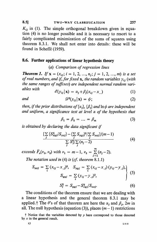
8.5] TWO-WAY CLASSIFICATION 257
Ki; in (1). The simple orthogonal breakdown given in equa-tion (4) is no longer possible and it is necessary to resort to afairly complicated minimization of the sums of squares usingtheorem 8.3.1. We shall not enter into details: these will befound in Scheffe (1959).
8.6. Further applications of linear hypothesis theory
(a) Comparison of regression lines
Theorem 1. If x = (xi;; i = 1, 2, ..., n;; j = 1, 2, ..., m) is a setof real numbers, and if, for fixed x, the random variables yi; (withthe same ranges of suffixes) are independent normal random vari-ables with 6'(y, I x) = a, + fl (xi, - x) (1)
and 92(yi, I x) = 0; (2)
then, if the prior distributions of {a1}, {,6,} and In 0 are independentand uniform, a significance test at level a of the hypothesis that
11 = 12 = ... = Nm (3)
is obtained by declaring the data significant if
[E {Sxv,lSxxf} -{I S ,f}2/E Sxxf)I (m - 1)
I S2/E (n,-2)m
exceeds FF,(vl, v2) with v1 = m -1, v2 = E (n; - 2).j=1
The notation used in (4) is (cf. theorem 8.1.1)
(4)
S.., = Z (x, - x.,)2, Sxv, = E (xj - x.,) (yf -y.,),IiSvv, _ (y, -y.,)2,
(5)
Si = Svv, - Sxv,I Sxx, (6)
The conditions of the theorem ensure that we are dealing witha linear hypothesis and the general theorem 8.3.1 may beapplied. t The B's of that theorem are here the aj and j6j, 2m inall. The null hypothesis (equation (3)), places (m - 1) restrictions
t Notice that the variables denoted by y here correspond to those denotedby x in the general result.
iq LS 11
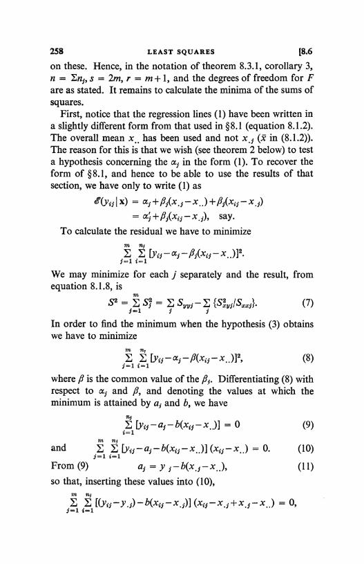
258 LEAST SQUARES [8.6
on these. Hence, in the notation of theorem 8.3.1, corollary 3,n = En j, s = 2m, r = m + 1, and the degrees of freedom for Fare as stated. It remains to calculate the minima of the sums ofsquares.
First, notice that the regression lines (1) have been written ina slightly different form from that used in §8.1 (equation 8.1.2).The overall mean x_, has been used and not x, j (x in (8.1.2)).The reason for this is that we wish (see theorem 2 below) to testa hypothesis concerning the aj in the form (1). To recover theform of §8.1, and hence to be able to use the results of thatsection, we have only to write (1) as
-ff(yij 1 x) = a j +/j(x.j - x..) +/3j(xij - x.j)
= xj +Nj(xij -x.j), say.
To calculate the residual we have to minimizem of
E E [yij-,7j-Rj(xij-x..)]2.j=1 i=1
We may minimize for each j separately and the result, fromequation 8.1.8, is
mS2 = jE SS = E Svvj - E {Sxvj/Sxzj}. (7)
In order to find the minimum when the hypothesis (3) obtainswe have to minimize
m Win,,
r,, RE Lyij-aj-N(xij-x..)]2, (8)j=1 i=1
where /3 is the common value of the /3j. Differentiating (8) withrespect to aj and /3, and denoting the values at which theminimum is attained by aj and b, we have
[yij-aj-b(xij-x.)] = 0 (9)i=1
m nj r''
and E E [ ij-aj-b(xij-x..)] (xij-x..) = 0. (10)j=1 i=1
From (9) aj = y j - b(x. j - (11)
so that, inserting these values into (10),m ny
E E [(yij-y.j)-b(xij-x.j)] (xij-x.j+x.5-x..) = 0,j=1 i=1
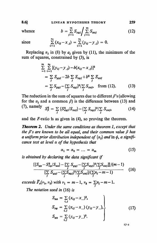
8.61 LINEAR HYPOTHESIS THEORY 259m
whence b =m
fE1Sxxf (12)
j=1 =ni ni
since (xv; - X. J) = E (y , -Y.j) = 0.i=1 ti=1
Replacing a; in (8) by aj given by (11), the minimum of thesum of squares, constrained by (3), is
m n;
E E [(Yzj-Y.j)-b(xjj-x.j)l2=1 i=1
_ Syy; - 2b 5 j + b2 S=j
= ESyy; -- {E Sxy1}2/ Sxx;, from (12). (13)j j I
The reduction in the sum of squares due to different,8's (allowingfor the a; and a common /3) is the difference between (13) and(7), namely S,2
6 = E {Sxvjl Sxxj} - {E Sx(14)and the F-ratio Is as given in (4), so proving the theorem.
Theorem 2. Under the same conditions as theorem 1, except thatthe fl's are known to be all equal, and their common value j6 hasa uniform prior distribution independent of {a;} and In 0, a signifi-cance test at level a of the hypothesis that
a1=a2=... =am
is obtained by declaring the data significant if
On - Syy/Sxx} - [E Syyf - {F1Syj}2/z,Sxxjll /(m - 1)
[E S,,,--{Zj S.YJ)2/ESxjl/(En;-m-1)
exceeds F2(v1, v2) with v1 = in -1, v2 = En; - m -1.
(15)
(16)
The notation used in (16) is
S. = E (xt;-x..)2,i.j
Sxy = E (xij-x..) (Yij-Y.), (17)
Syy = E (Yif -Y..)2.
17-2
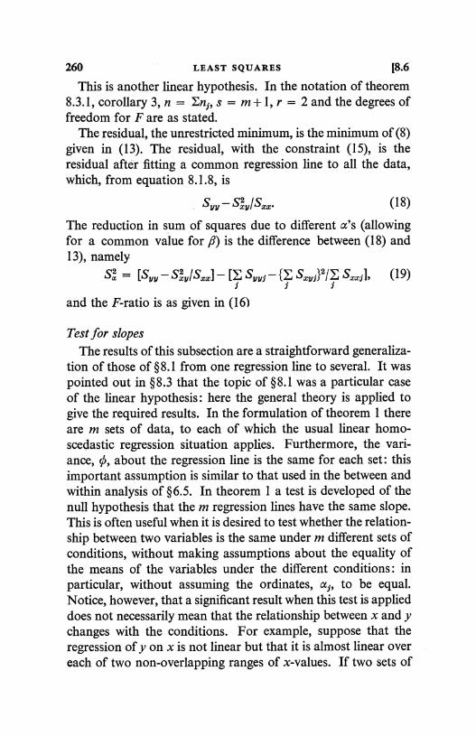
260 LEAST SQUARES [8.6
This is another linear hypothesis. In the notation of theorem8.3.1, corollary 3, n = Enf, s = m+ 1, r = 2 and the degrees offreedom for F are as stated.
The residual, the unrestricted minimum, is the minimum of (8)given in (13). The residual, with the constraint (15), is theresidual after fitting a common regression line to all the data,which, from equation 8.1.8, is
Svv - SSj/SS.. (18)
The reduction in sum of squares due to different a's (allowingfor a common value for 8) is the difference between (18) and13), namely
Sa = [Svv - S,/S] - [E SYj - {E Sam,,;}2/E Sjl , (19)
and the F-ratio is as given in (16)
Test for slopesThe results of this subsection are a straightforward generaliza-
tion of those of §8.1 from one regression line to several. It waspointed out in §8.3 that the topic of §8.1 was a particular caseof the linear hypothesis : here the general theory is applied togive the required results. In the formulation of theorem 1 thereare m sets of data, to each of which the usual linear homo-scedastic regression situation applies. Furthermore, the vari-ance, 0, about the regression line is the same for each set: thisimportant assumption is similar to that used in the between andwithin analysis of § 6.5. In theorem 1 a test is developed of thenull hypothesis that the m regression lines have the same slope.This is often useful when it is desired to test whether the relation-ship between two variables is the same under m different sets ofconditions, without making assumptions about the equality ofthe means of the variables under the different conditions: inparticular, without assuming the ordinates, a3, to be equal.Notice, however, that a significant result when this test is applieddoes not necessarily mean that the relationship between x and ychanges with the conditions. For example, suppose that theregression of y on x is not linear but that it is almost linear overeach of two non-overlapping ranges of x-values. If two sets of
8.6] LINEAR HYPOTHESIS THEORY 261
data have x-values in the different ranges then the regressioncoefficients will differ. To avoid such troubles the x-valuesshould be about the same in each set: but the test is still satis-factory even if they are not; it is the interpretation of it thatrequires attention.
Test for ordinates
If the slopes of the regression lines are unequal, the differencebetween the ordinates changes with the value of x. But in thespecial case of equal slopes, the differences in ordinates are thesame for all x-values. It is then of interest to know if theordinates differ. Theorem 2 enables this equality to be tested.Notice that both tests involve the sums of squares and productswithin each set S.,,,, Sxy; and Syyj (equations (5)), and the latteralso involves the total sums of squares and products Sxx, Sxand SQL (equations (17)) obtained by pooling all the data. Fromthe fundamental relationship expressed in equation 6.5.1, heregeneralized to the case of unequal sample sizes, the total may beexpressed as the sum of the within and the between: thus,
Sxx = E Sxxf+E nf(x.3-x..)2 (20)
(with a similar expression with y in place of x) and
S.y = E Sxv.7+E n,(x.5-x..) (y.j-y..). (21)
Analysis of varianceBoth tests may be incorporated into an analysis of variance
table, but since the two reductions, Sa and S,16, are not ortho-gonal some care must be exercised, as explained in § 8.3.Table 8.6.1 shows the arrangement. The total sum of squares isthat about the common line-the values of which we do not wishto test. This may be reduced, first by fitting different ordinatesand then by fitting different slopes. The first breaks the total upinto Sa for the ordinates and S2 + S,16. The second breaks thelatter up into S2 (equation (7)) and S,26. The title `between slopessum of squares', S,26, is an abbreviation for the reduction due todifferent slopes (allowing for different a's and /1). The title`between ordinates sum of squares', Sa, is an abbreviation for
262 LEAST SQUARES [8.6
the reduction due to different ordinates (allowing for a commonline). This is not equal to the reduction due to different ordinates(allowing for different /3's and a); as explained above this is notusually of interest. What one usually does is to test for the slopes(theorem 1) first. If this is not significant one can test for theordinates, acting as if the slopes were the same. The point beingthat there is a natural ordering of the parameters here: the a'snaturally occurring first in the reduction, before the ,B's.
TABLE 8.6.1
Sums ofsquares
Degrees offreedom Mean squares F
Between SS2 m-1 s.2 = SS/(m-1) s.2/''ordinates
Between S,92 m-1 sR2 = Sy2/(m-1) sg2/s2
slopesResidual S2 E(nf - 2) s2 = S2/E(n, - 2) -Ordinates S2+SS2 En,-m-1 s = (S2+S2s)l(En,-m-i) -residual
Total 5,,,,-S'n,/Sxx Enf-2 - -(b) Analysis of covariance
Theorem 3. Let R(x, x) denote the residual sum of squares fromthe linear hypothesis (in the notation of §8.3)
1(x) = AO or 1(x1) = E a1, 6 f. (22)
From equation 8.3.28
R(x, x) = x'x-x'A(A'A)-'A'x. (23)
Then if the linear hypothesis
1°(x) = A9 + ftz or (o (xi) = E aif B3 +,8zi (24)
is considered, the residual sum of squares is
R(x, X) - R(x, z)2/R(z, z). (25)
(Here fl is an additional parameter and z is a known vector linearlyindependent of the columns of A.)
The expression to be minimized is
(x - A6 -,Bz)' (x - AO -,az).
8.61 LINEAR HYPOTHESIS THEORY 263
Let us minimize it in two stages, first with respect to 0 forfixed /3, and then with respect to 8. If y = x-/3z the first stagegives
R(y, y) = y'y-y'A(A'A)-1A'y= (x - /3z)' (x -,Bz) - (x -/3z)' A(A'A)-IA'(x -ftz),
which is a quadratic in /3,
R(x, x) - 2fR(x, z) +#2R(z, z),
with minimum at b = R(x, z)/R(z, z) and minimum value givenby (25).
Use of analysis of covariance
This theorem describes how the residual sum of squares isreduced by the introduction of a single additional parameter, /3,and, as such, gives an alternative test for this single parameter /3which is identical with that obtained in corollary 2 to theorem8.3.1. The corollary is the most convenient form when this test isrequired: the present form is more suitable in a connexion nowto be described.
The term `analysis of covariance' is a rather loose one.`Analysis of variance' most commonly refers to the case of adesign matrix A having specially simple properties (usuallyorthogonality with respect to sets of parameters) such as wasdiscussed in § 8.5. The matrix A is truly designed, that is theelements are known before experimentation, unlike the elementsin the design matrix A of the multiple regression situation of§8.4 which, depending on the x's (in the notation of that section),are not systematic. Analysis of covariance usually refers to themodel given in (24), where A is truly designed and z is (irrele-vantly) random. Some, or all, of the 9's are of interest, 6 is not.The situation arises when one is investigating the dependenceof x on certain factors, expressed in the 0's, but x is also knownto be influenced by another quantity z. Thus, in an experimentto investigate the effect of type of wool and type of machine onthe breakage rate in spinning textile yarn, a two-way classifica-tion as in § 8.5 might be used with these two factors. However,the breakage rate is obviously affected by the weight per unit
264 LEAST SQUARES [8.6
length of yarn, a variable which it is difficult to control. Ananalysis of covariance might therefore be used, based on themodel in (24), with the weight as the `z' variable.
Regression reduction
The calculations necessary for an analysis of covariancefollow directly from those for the corresponding analysis ofvariance, in which the z-variable is omitted, by using theorem 3.Suppose the 6's are divided into two groups, called the first andsecond, and it is desired to test the hypothesis that those in thesecond group are all zero. Then in the analysis of varianceSl - S12 must be compared with S12 (the notation is as in § 8.3).In the analysis of covariance S2 - 512 must be compared with1,6 ,8
S12ft, where S12 is the residual fitting both groups and ft, andSla similarly. But both S2 and Sla are easily obtained fromS2 Sl respectively by use of theorem 3.
The quantity R(x, x) is the residual for the x's with ft = 0.R(z, z) is the same expression with z replacing x. R(x, z) is thesame expression with every squared x replaced by a product ofan x with its corresponding z. Consequently, if we calculate theanalysis of variance for x and add the similar analysis for z andfor the product of x and z, we shall have all the terms necessaryfor (25). The operation of subtracting R(x, z)2/R(z, z) from theoriginal residual to obtain the new one will be called theregression reduction. Both S12fi and Sla can be obtained fromS2 Sl respectively by regression reduction. Table 8.6.2 showshow the calculations may be laid out for the two-way classifica-tion in order to test the interaction. The notation correspondsto that of table 8.5.1 with additions to make clear whichvariable is being used: only the sums of squares and productsare included. Arrows show the order in which the terms arecalculated. Thus S! j(x) denotes K (xi f - X,.. - x )2 andso SZ j(x, z) denotes
i.1
K E (xi1.-xi..-x.5.+x...) (zi1.-zi..-z.f.+Z...)i,
The interaction effects and the residuals are added together togive the minima of the sums of squares with zero interaction,
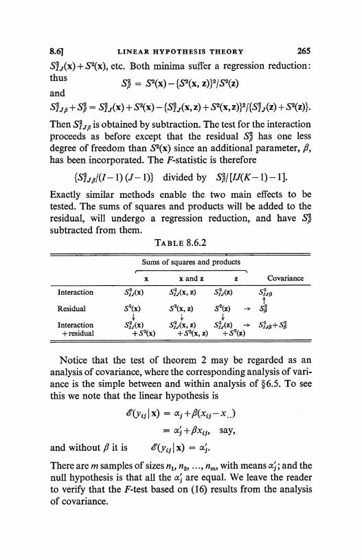
8.61 LINEAR HYPOTHESIS THEORY 265
S! j(x) + S2(x), etc. Both minima suffer a regression reduction:thus 2 2 2
2 2and
a) = 3 \X, Z)} /S (Z)(X) - 13
SZJf + SJ = Sj(x) + S2(X) - {Si j(X, Z) + S2(X, Z)}2/{SIJ(Z) + S2(Z)}.
Then SIJfl is obtained by subtraction. The test for the interactionproceeds as before except that the residual SS has one lessdegree of freedom than S2(x) since an additional parameter, ,G,has been incorporated. The F-statistic is therefore
{S1Jft/(I-1) (J- 1)} divided by S,26/[IJ(K-1)-1].
Exactly similar methods enable the two main effects to betested. The sums of squares and products will be added to theresidual, will undergo a regression reduction, and have S,28subtracted from them.
TABLE 8.6.2
Sums of squares and products
x x and z z Covariance
InteractionS12.1(x) SIJ(x, Z) S7 (z) SSjy
Residual S2(x) S2(x, Z) S2(z) - tSs
Interaction St (x)1
,(x, z)SI1
5" ,(z) - +Ss+ residual +S2(x)
,
+S2(x, Z),+S2(z)
Notice that the test of theorem 2 may be regarded as ananalysis of covariance, where the corresponding analysis of vari-ance is the simple between and within analysis of §6.5. To seethis we note that the linear hypothesis is
.e(yz, I x) = ai +/3(xi; - x..)
of +,6x2 , say,
and without fl it is 40(yif I x) = a;.
There are m samples of sizes n1, n2i ..., nm, with means af; and thenull hypothesis is that all the aj are equal. We leave the readerto verify that the F-test based on (16) results from the analysisof covariance.
266 LEAST SQUARES 18.6
(c) Polynomial regression
There are many situations, where the relationship betweentwo variables is being considered, in which the regressionf(y (x) is not linear and the results of §8.1 are inadequatebecause of curvature in the regression. Indeed, one of the oldestof statistical problems is that of `fitting a curve to data'; that is,to a set of (x, y)-points. In modern language we consider a setx = (x1, x2, ..., x.) and suppose that for fixed x the randomvariables y1, y2, ..., y,, are independent normal variables with
.ff(Yi(x) = ap+aixi+a2xi+...+akxs (26)
and _92(yi (x) = 0. (27)
The assumptions are those of homoscedastic (equation (27))normal regression of polynomial form. If the a; and lno haveindependent uniform prior distributions, then the model is inthe standard linear hypothesis form with 0' = (ao, a,, ..., ak)and a design matrix with ith row (1, xi, xi, ..., x?). In view ofthe general form of the design matrix the general computationalmethods of §8.4 have to be used; and we perform a multiplelinear regression on the quantities x, x2, ..., xk. (In the notationof equation 8.4.7, xij = xz.) It was pointed out in that sectionthat the order in which the variables were introduced wasimportant because it affected the significance tests that couldeasily be performed. In polynomial regression there is a naturalorder, namely that of increasing powers of x. The parameterswill then be introduced in the order ao, a,, ..., ak and it ispossible to test that a8+i = a8+2 = ... = ak = 0 for any s. Thisprovides a test that, given the polynomial is at most of degree k,it is of degree at most s. Usual practice is to take s = k - 1;that is, to test whether ak = 0. If this is not significant then k isreduced by one and one tests whether ak_1 = 0, finishing upwith the polynomial of least degree not exceeding k. The testsare easily carried out since the reduction in sum of squares dueto including a8, allowing for ao, al, ..., a8_1 is, in the notation ofthe computational scheme of § 8.4, simply o),2, (stage (4) of thecomputation). When a test is significant then the polynomial of
8.61 LINEAR HYPOTHESIS THEORY 267
that degree must be used, and the estimates of the coefficients zhave, for fixed 0, a dispersion matrix given by the inversematrix B-1 (in the notation again of §8.4) of the order corre-sponding to the degree of the polynomial.
A difficulty here is knowing what value of k to use to start.Even if the tests of as, as+I, ..., ak are all insignificant there isalways the possibility that the inclusion of a term of higherdegree than k would result in an even better 'fit': or, in modernlanguage, would reduce the residual sum of squares appreciably.The key to this problem lies in the form of this residual. In anyof these tests (03 is compared with the residual, which is the sumof squares of deviations about the curve of best `fit' of degrees.Therefore, rather loosely, the tests compare whether the intro-duction of x8 results in an appreciable reduction compared withwhat remains, but there is no way of judging whether whatremains is adequate. The situation is most satisfactorily resolvedif the value of 0 is known, equal to 0'2. In this case corollary 1to theorem 8.3.1 may be used, in conjunction with the methodof § 5.3, to test the adequacy of the `fit'. For, if the correctdegree of polynomial has been used a test of the null hypothesisthat 0 = a2 should be nonsignificant. Consequently, when0 = 0-2, the powers of x may be introduced in ascending orderuntil the residual sum of squares is compatible with the knownamount of variation, 0-2. It would be pointless to attempt toimprove the `fit' so that the residual was less than the knownrandom error. This method may be modified if an independentestimate of ¢ is available such that c/o, for appropriate c, has aX2-distribution. (Such an estimate results from most normaldistribution situations as we have repeatedly seen.) The x2-testfrom § 5.3, used above, may then be replaced by the F-test of§6.2, to compare the two estimates of variance: one from theresidual and the other independent one.
Orthogonal polynomialsOne unpleasant feature of the polynomial regression, in the
form of equation (26), is that if the degree of the polynomial ischanged, say from s to s -1, then all the estimates of the para-meters will, in general, be changed. This is because the design is
268 LEAST SQUARES [8.6
not orthogonal and just as a test for ai will be influenced by howmany other a's have been allowed for, so will the posterior dis-tribution of ai be similarly changed. A way out of this difficultyis to rewrite equation (26) in the form
/e(Yi I X) = foPo(xi) +fl1P1(xi) +N2P2(xi) + ... +NkPk(xi), (28)
where P8(x) is a known polynomial of degree s in x, to bedetermined. Equation (26) is the special case P,8(x) = x8. Thedesign matrix, A, now has typical row (P0(xi), P1(xi), ..., Pk(xi))
nand the elements of A'A are E Pi(xu) P;(xu). Suppose that the
u=1
polynomials are chosen so thatnE Pi(xu) P,(xu) = 0 (i + D. (29)
U=1
Then A'A is a diagonal matrix and (see equation 8.3.26) thedesign is orthogonal with respect to each of the parametersseparately. Consequently if the degree of the polynomial (28)is increased from k to k + 1 none of the fl's in (28) is altered.Such polynomials are called orthogonal polynomials.
It remains to show that orthogonal polynomials exist. Po(x)may be put equal to 1. Then P1(x) must satisfy (29) with i = 0,j = 1. If P1(x) = ax + b, for some a and b, this gives
nE (ax,+b) = 0U=1
which is satisfied, for example, by
a = 1, b = - E xu/n = x.U=1
Hence, if k = 1, (28) becomes
ff(Yi I X) = flo +Q1(xi - x),
exactly the form used in § 8.1. Indeed the term - ,8x was intro-duced into equation 8.1.2 so that the estimates of a and,6 shouldbe orthogonal and the posterior distributions of a and f be inde-pendent, given 0. Suppose Po(x), ..., Pa_1(x) have been found:we show how P8(x) can be found. Since P8(x) is a polynomial ofdegree x8 it may be written
P8(x) = a8x8 + a8-1P8-1(x) + a8-2P8-2(x) + ... + aoPo(x), (30)
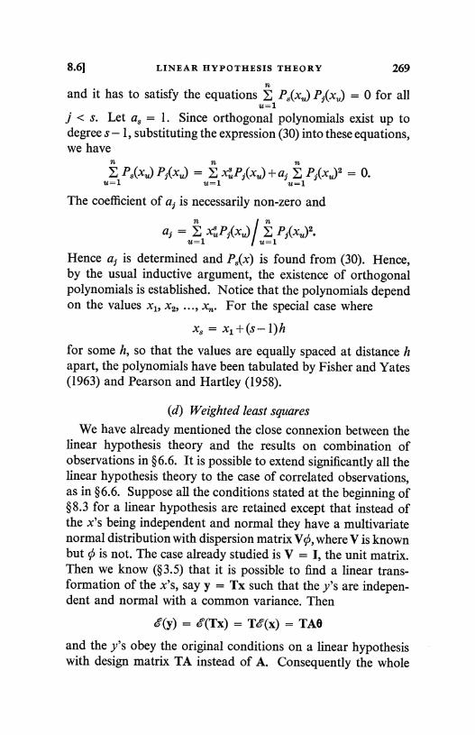
8.61 LINEAR HYPOTHESIS THEORY 269
and it has to satisfy the equations P3(xu) P2(xu) = 0 for allu=1
j < s. Let a3 = 1. Since orthogonal polynomials exist up todegree s - 1, substituting the expression (30) into these equations,we have
n n nE P3(xu) P1(xu) = E xuP1(xu)+af E P,(xu)2 = 0.U=1 u=1 u=1
The coefficient of a; is necessarily non-zero and
a; = E xuP1(xu)/ E P1(xx)2.u=1 u=1
Hence a; is determined and P3(x) is found from (30). Hence,by the usual inductive argument, the existence of orthogonalpolynomials is established. Notice that the polynomials dependon the values x1, x2, ..., xn. For the special case where
x3 = x1+(s-1)h
for some h, so that the values are equally spaced at distance hapart, the polynomials have been tabulated by Fisher and Yates(1963) and Pearson and Hartley (1958).
(d) Weighted least squares
We have already mentioned the close connexion between thelinear hypothesis theory and the results on combination ofobservations in §6.6. It is possible to extend significantly all thelinear hypothesis theory to the case of correlated observations,as in § 6.6. Suppose all the conditions stated at the beginning of§8.3 for a linear hypothesis are retained except that instead ofthe x's being independent and normal they have a multivariatenormal distribution with dispersion matrix V¢, where V is knownbut 0 is not. The case already studied is V = I, the unit matrix.Then we know (§3.5) that it is possible to find a linear trans-formation of the x's, say y = Tx such that the y's are indepen-dent and normal with a common variance. Then
i(y) = ff(Tx) = T.-(x) = TAO
and the y's obey the original conditions on a linear hypothesiswith design matrix TA instead of A. Consequently the whole
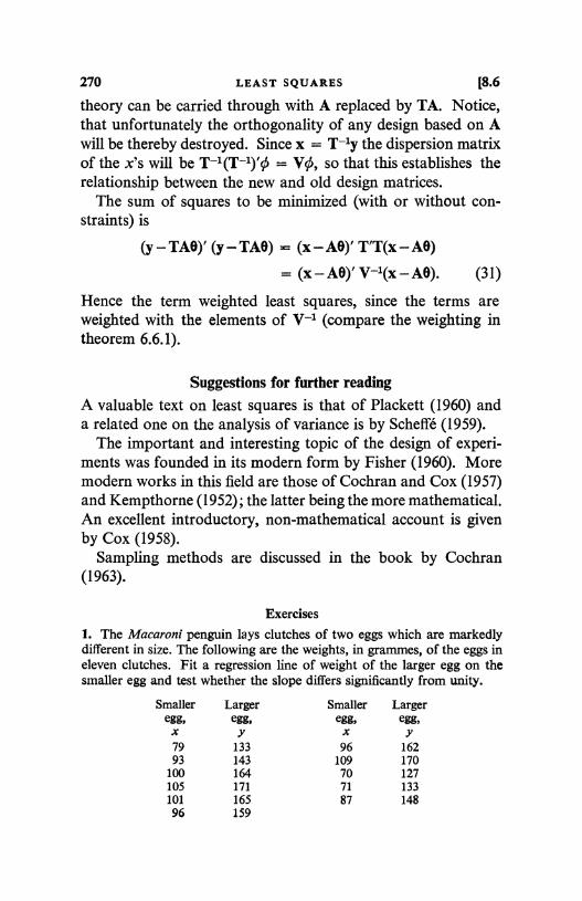
270 LEAST SQUARES [8.6
theory can be carried through with A replaced by TA. Notice,that unfortunately the orthogonality of any design based on Awill be thereby destroyed. Since x = T-1y the dispersion matrixof the x's will be T-1(T-1)'q = Vg, so that this establishes therelationship between the new and old design matrices.
The sum of squares to be minimized (with or without con-straints) is
(y - TAO)' (y - TAO) _ (x - AO)' T'T(x - AO)
= (x-AO)' V-1(x-AO). (31)
Hence the term weighted least squares, since the terms areweighted with the elements of V-1 (compare the weighting intheorem 6.6.1).
Suggestions for further reading
A valuable text on least squares is that of Plackett (1960) anda related one on the analysis of variance is by Scheffe (1959).
The important and interesting topic of the design of experi-ments was founded in its modern form by Fisher (1960). Moremodern works in this field are those of Cochran and Cox (1957)and Kempthorne (1952); the latter being the more mathematical.An excellent introductory, non-mathematical account is givenby Cox (1958).
Sampling methods are discussed in the book by Cochran(1963).
Exercises
1. The Macaroni penguin lays clutches of two eggs which are markedlydifferent in size. The following are the weights, in grammes, of the eggs ineleven clutches. Fit a regression line of weight of the larger egg on thesmaller egg and test whether the slope differs significantly from unity.
Smalleregg,
x
Largeregg,
y
Smalleregg,
x
Largeregg,
y79 133 96 162
93 143 109 170
100 164 70 127
105 171 71 133
101 165 87 148
96 159
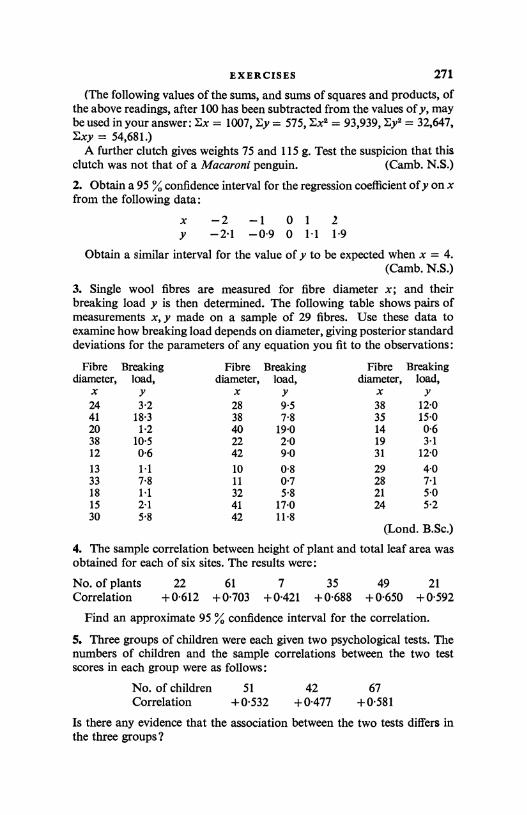
EXERCISES 271
(The following values of the sums, and sums of squares and products, ofthe above readings, after 100 has been subtracted from the values of y, maybe used in your answer: Ex = 1007, Ey = 575, Ex2 = 93,939, Eye = 32,647,Exy = 54,681.)
A further clutch gives weights 75 and 115 g. Test the suspicion that thisclutch was not that of a Macaroni penguin. (Camb. N.S.)
2. Obtain a 95 % confidence interval for the regression coefficient of y on xfrom the following data:
x -2 -1 0 1 2y -2-1 -0-9 0 1.1 1.9
Obtain a similar interval for the value of y to be expected when x = 4.(Camb. N.S.)
3. Single wool fibres are measured for fibre diameter x; and theirbreaking load y is then determined. The following table shows pairs ofmeasurements x, y made on a sample of 29 fibres. Use these data toexamine how breaking load depends on diameter, giving posterior standarddeviations for the parameters of any equation you fit to the observations:
Fibrediameter,
x
Breaking
load,y
Fibrediameter,
x
Breaking
load,y
Fibrediameter,
x
Breakingload,y
24 3.2 28 9.5 38 12.041 18.3 38 7.8 35 15.020 1.2 40 19.0 14 0.638 10.5 22 2.0 19 3.112 0.6 42 9.0 31 12.0
13 1.1 10 0.8 29 4.033 7.8 11 0.7 28 7.118 1.1 32 5.8 21 5.015 2.1 41 17.0 24 5.230 5.8 42 11.8
(Lond. B.Sc.)
4. The sample correlation between height of plant and total leaf area wasobtained for each of six sites. The results were:
No. of plants 22 61 7 35 49 21Correlation +0.612 +0.703 +0.421 +0.688 +0.650 +0.592
Find an approximate 95 % confidence interval for the correlation.
5. Three groups of children were each given two psychological tests. Thenumbers of children and the sample correlations between the two testscores in each group were as follows:
No. of children 51 42 67Correlation +0.532 +0.477 +0.581
Is there any evidence that the association between the two tests differs inthe three groups?
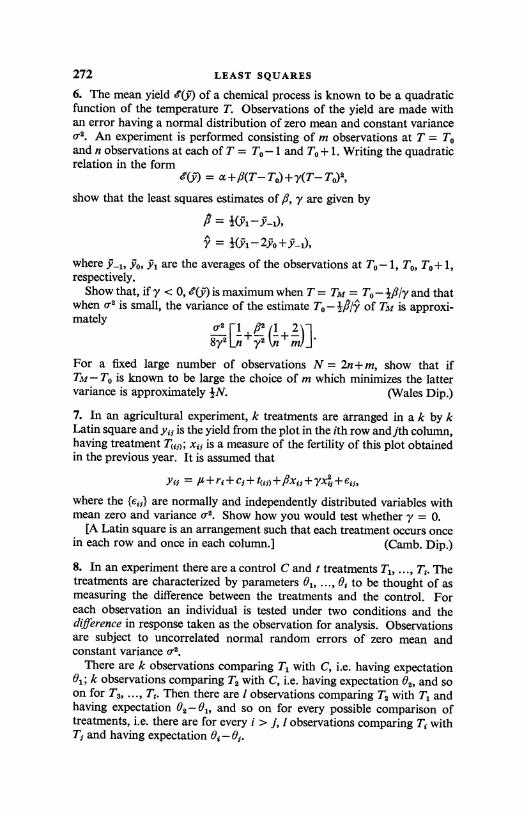
272 LEAST SQUARES
6. The mean yield f(y-) of a chemical process is known to be a quadraticfunction of the temperature T. Observations of the yield are made withan error having a normal distribution of zero mean and constant varianceQ2. An experiment is performed consisting of m observations at T = Toand n observations at each of T = To-1 and To+ 1. Writing the quadraticrelation in the form
a+fl(T-To)+y(T-To)2,show that the least squares estimates of /3, y are given by
ft _ l(.vl-Y-D,
where Y_1i Yo, Yl are the averages of the observations at To-1, To, To+ 1,respectively.
Show that, if y < 0, e'(y-) is maximum when T = Tm = To -1,6/y and thatwhen 0-2 is small, the variance of the estimate To-Jft/y of Tm is approxi-mately
8y2Ln+6
2 Vt+ml1'
For a fixed large number of observations N= 2n+m, show that ifTm-To is known to be large the choice of m which minimizes the lattervariance is approximately IN. (Wales Dip.)
7. In an agricultural experiment, k treatments are arranged in a k by kLatin square and yt, is the yield from the plot in the ith row andjth column,having treatment Tctn; xtl is a measure of the fertility of this plot obtainedin the previous year. It is assumed that
yo = A+ri+cf+tw)-}-/3xJ+y4i +er,where the {e, j are normally and independently distributed variables withmean zero and variance a2. Show how you would test whether y = 0.
[A Latin square is an arrangement such that each treatment occurs oncein each row and once in each column.] (Camb. Dip.)
8. In an experiment there are a control C and t treatments T1, ..., Tt. Thetreatments are characterized by parameters 01, ..., Bt to be thought of asmeasuring the difference between the treatments and the control. Foreach observation an individual is tested under two conditions and thedifference in response taken as the observation for analysis. Observationsare subject to uncorrelated normal random errors of zero mean andconstant variance 0-2.
There are k observations comparing T1 with C, i.e. having expectation0l; k observations comparing T2 with C, i.e. having expectation 02i and soon for T3, ..., Tt. Then there are I observations comparing T. with T1 andhaving expectation 02 - 01, and so on for every possible comparison oftreatments, i.e. there are for every i > j, I observations comparing T{ withTs and having expectation Bt - 0,.
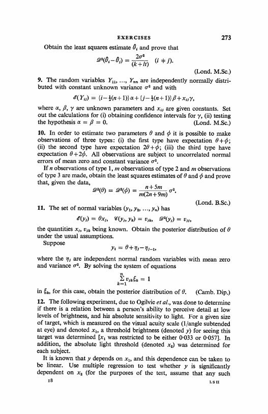
EXERCISES
Obtain the least squares estimate B; and prove that
_q2(8.-81) (k+lt) (I
273
(Lond. M.Sc.)9. The random variables Y11, ..., Y,,,, are independently normally distri-buted with constant unknown variance r2 and with
-ff(Y;j) = {i-j;(n+1)}a+{j-j;(n+l)}fl+x15y,
where a, /3, y are unknown parameters and x,, are given constants. Setout the calculations for (i) obtaining confidence intervals for y, (ii) testingthe hypothesis a = 8 = 0. (Lond. M.Sc.)
10. In order to estimate two parameters 0 and 0 it is possible to makeobservations of three types: (i) the first type have expectation 0+0;(ii) the second type have expectation 20+0; (iii) the third type haveexpectation 0+20. All observations are subject to uncorrelated normalerrors of mean zero and constant variance 0.
If n observations of type 1, m observations of type 2 and m observationsof type 3 are made, obtain the least squares estimates of 0 and ¢ and provethat, given the data,
n+5m2(B) _ m(2n+9m) 2.
11. The set of normal variables (.YI, y21 ..., has
-ff(Yj) = OxJ, `'(Yv Yk) = Vik, -92(Ys) = VJJ,
(Lond. B.Sc.)
the quantities x5, VJk being known. Obtain the posterior distribution of 9under the usual assumptions.
Supposeyt = 9+V1-71J-1,
where the Va are independent normal random variables with mean zeroand variance o-1. By solving the system of equations
nE VfkCCSk = 1
k=1
in Sk, for this case, obtain the posterior distribution of 0. (Camb. Dip.)
12. The following experiment, due to Ogilvie et al., was done to determineif there is a relation between a person's ability to perceive detail at lowlevels of brightness, and his absolute sensitivity to light. For a given sizeof target, which is measured on the visual acuity scale (1/angle subtendedat eye) and denoted x1, a threshold brightness (denoted y) for seeing thistarget was determined [x1 was restricted to be either 0.033 or 0.057]. Inaddition, the absolute light threshold (denoted x2) was determined foreach subject.
It is known that y depends on x1, and this dependence can be taken tobe linear. Use multiple regression to test whether y is significantlydependent on x2 (for the purposes of the test, assume that any such
18 LS II
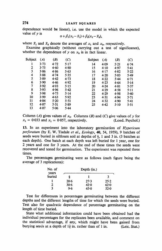
274 LEAST SQUARES
dependence would be linear), i.e. use the model in which the expectedvalue of y is
a+/31(x1-1)+/32(xa-x2),
where x'1 and xa denote the averages of xl and x2, respectively.Examine graphically (without carrying out a test of significance),
whether the dependence of y on xa is in fact linear.
Subject (A) (B) (C) Subject (A) (B) (C)
1 3.73 4.72 5.17 14 4.09 5.21 6.742 3.75 4.60 4.80 15 4.10 4.97 5.413 3.86 4.86 5.63 16 4.17 4.82 5.22
4 3.88 4.74 5.35 17 4.20 5.03 5.495 3.89 4.42 4.73 18 4.22 5.44 6.716 3.90 4.46 4.92 19 4.23 4.64 5.14
7 3.92 4.93 5.15 20 4.24 4.81 5.37
8 3.93 4.96 5.42 21 4.29 4.58 5.119 3.98 4.73 5.14 22 4.29 4.98 5.4010 3.99 4.63 5.92 23 4.31 4.94 5.71
11 4.04 5.20 5.51 24 4.32 4.90 5.4112 4.07 5.31 5.89 25 4.42 5.10 5.5113 4.07 5.06 5.44
Column (A) gives values of x2. Columns (B) and (C) give values of y forxl = 0.033 and xl = 0.057, respectively. (Lond. Psychol.)
13. In an experiment into the laboratory germination of Hypericumperforatum (by E. W. Tisdale et al., Ecology, 40, 54, 1959), 9 batches ofseeds were buried in siltloam soil at depths of 1, 1 and 3 in. (3 batches ateach depth). One batch at each depth was left buried for 1 year, one for2 years and one for 3 years. At the end of these times the seeds wererecovered and tested for germination. The experiment was repeated threetimes.
The percentages germinating were as follows (each figure being theaverage of 3 replications):
No. of Depth (in.)yearsburied 3- 1 3
1 20.6 27.3 25.22 30.6 42.0 62.03 9.6 45.0 52.0
Test for differences in percentages germinating between the differentdepths and the different lengths of time for which the seeds were buried.Test also for quadratic dependence of percentage germinating on thelength of time buried.
State what additional information could have been obtained had theindividual percentages for the replicates been available, and comment onthe statistical advantage, if any, which might have been gained fromburying seeds at a depth of 1J in. rather than of 1 in. (Leic. Stat.)
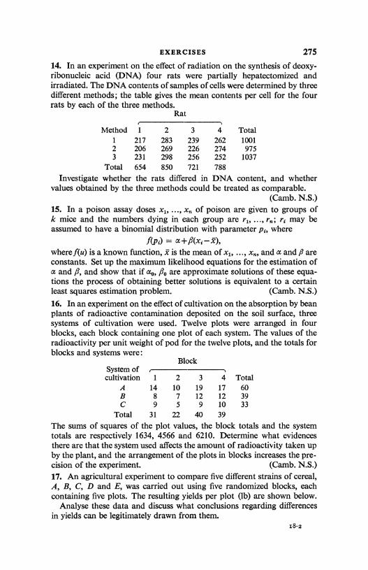
EXERCISES 275
14. In an experiment on the effect of radiation on the synthesis of deoxy-ribonucleic acid (DNA) four rats were partially hepatectomized andirradiated. The DNA contents of samples of cells were determined by threedifferent methods; the table gives the mean contents per cell for the fourrats by each of the three methods.
Rat
Method 1 2 3 4 Total1 217 283 239 262 1001
2 206 269 226 274 975
3 231 298 256 252 1037
Total 654 850 721 788
Investigate whether the rats differed in DNA content, and whethervalues obtained by the three methods could be treated as comparable.
(Camb. N.S.)15. In a poison assay doses x1, ..., x of poison are given to groups ofk mice and the numbers dying in each group are r1, ..., r,,; ri may beassumed to have a binomial distribution with parameter pi, where
f(pi) = a+,6(xc-x),where f(u) is a known function, x is the mean of x1, ..., x,,, and a and,6 areconstants. Set up the maximum likelihood equations for the estimation ofa and f3, and show that if ao, fto are approximate solutions of these equa-tions the process of obtaining better solutions is equivalent to a certainleast squares estimation problem. (Camb. N.S.)
16. In an experiment on the effect of cultivation on the absorption by beanplants of radioactive contamination deposited on the soil surface, threesystems of cultivation were used. Twelve plots were arranged in fourblocks, each block containing one plot of each system. The values of theradioactivity per unit weight of pod for the twelve plots, and the totals forblocks and systems were:
BlockSystem ofcultivation 1 2 3 4 Total
A 14 10 19 17 60B 8 7 12 12 39
C 9 5 9 10 33
Total 31 22 40 39
The sums of squares of the plot values, the block totals and the systemtotals are respectively 1634, 4566 and 6210. Determine what evidencesthere are that the system used affects the amount of radioactivity taken upby the plant, and the arrangement of the plots in blocks increases the pre-cision of the experiment. (Camb. N.S.)17. An agricultural experiment to compare five different strains of cereal,A, B, C, D and E, was carried out using five randomized blocks, eachcontaining five plots. The resulting yields per plot (lb) are shown below.
Analyse these data and discuss what conclusions regarding differencesin yields can be legitimately drawn from them.
18-2
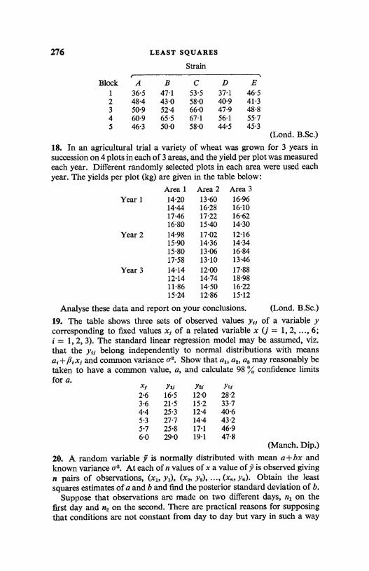
276 LEAST SQUARES
Strain
Block A B C D E1 36.5 47.1 53.5 37.1 46-52 48.4 43.0 58.0 40.9 41.33 50-9 52-4 66.0 47.9 48.84 60.9 65.5 67.1 56.1 55.75 46-3 50.0 58-0 44.5 45.3
(Lond. B.Sc.)
18. In an agricultural trial a variety of wheat was grown for 3 years insuccession on 4 plots in each of 3 areas, and the yield per plot was measuredeach year. Different randomly selected plots in each area were used eachyear. The yields per plot (kg) are given in the table below:
Area 1 Area 2 Area 3Year 1 14.20 13.60 16.96
14.44 16-28 16-1017.46 17-22 16.6216.80 15.40 14-30
Year 2 14.98 17-02 12-1615-90 14-36 14-3415-80 13-06 16-8417-58 13-10 13.46
Year 3 14.14 12.00 17.8812-14 14.74 18-9811.86 14-50 16-221524 12-86 15-12
Analyse these data and report on your conclusions. (Lond. B.Sc.)
19. The table shows three sets of observed values yip of a variable ycorresponding to fixed values x3 of a related variable x (j = 1, 2,..., 6;i = 1, 2, 3). The standard linear regression model may be assumed, viz.that the yip belong independently to normal distributions with meansai+/fixp and common variance 0.2. Show that a1, a2, ag may reasonably betaken to have a common value, a, and calculate 98 % confidence limitsfor a.
Xf Yxp Yap Yap
2-6 16-5 12.0 28-23-6 21.5 15-2 33.7
4.4 25.3 12-4 40.65-3 27.7 14-4 43-25.7 25-8 17-1 46.96-0 29-0 19.1 47-8
(Manch. Dip.)
20. A random variable y" is normally distributed with mean a+bx andknown variance 0-2. At each of n values of x a value of .P is observed givingn pairs of observations, (x1, y1), (x2, y2), ..., (x,, Obtain the leastsquares estimates of a and b and find the posterior standard deviation of b.
Suppose that observations are made on two different days, n1 on thefirst day and n2 on the second. There are practical reasons for supposingthat conditions are not constant from day to day but vary in such a way
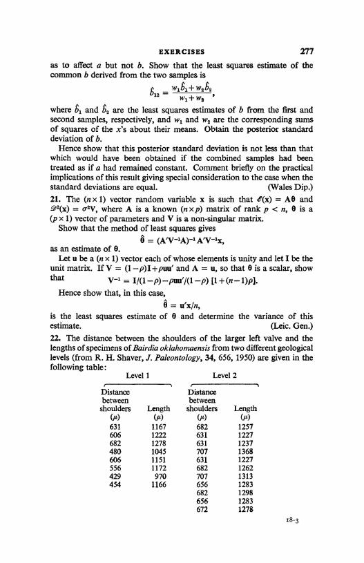
EXERCISES 277
as to affect a but not b. Show that the least squares estimate of thecommon b derived from the two samples is
wltl+w2t2S12 = Wl+w2
where 61 and & are the least squares estimates of b from the first andsecond samples, respectively, and w1 and w2 are the corresponding sumsof squares of the x's about their means. Obtain the posterior standarddeviation of b.
Hence show that this posterior standard deviation is not less than thatwhich would have been obtained if the combined samples had beentreated as if a had remained constant. Comment briefly on the practicalimplications of this result giving special consideration to the case when thestandard deviations are equal. (Wales Dip.)
21. The (n x 1) vector random variable x is such that -ff(x) = AO and_92(x) = U 2V' where A is a known (n x p) matrix of rank p < n, 0 is a(p x 1) vector of parameters and V is a non-singular matrix.
Show that the method of least squares gives
6 = (A'V-'A)-'AN-lx,as an estimate of 0.
Let u be a (n x 1) vector each of whose elements is unity and let I be theunit matrix. If V = (1-p)I+puu' and A = u, so that 0 is a scalar, showthat V-1 = I/(1-p)-puu'/(l -p) h+(n-1)pJ.
Hence show that, in this case,6 = u'x/n,
is the least squares estimate of 6 and determine the variance of thisestimate. (Leic. Gen.)
22. The distance between the shoulders of the larger left valve and thelengths of specimens of Bairdia oklahomaensis from two different geologicallevels (from R. H. Shaver, J. Paleontology, 34, 656, 1950) are given in thefollowing table:
Level 1 Level 2
Distance Distancebetween betweenshoulders Length shoulders Length
(F) (p) (A) (/a)631 1167 682 1257
606 1222 631 1227
682 1278 631 1237
480 1045 707 1368
606 1151 631 1227
556 1172 682 1262
429 970 707 1313
454 1166 656 1283
682 1298
656 1283
672 1278
18-3
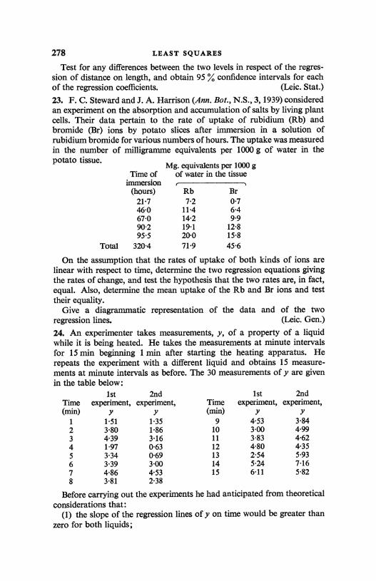
278 LEAST SQUARES
Test for any differences between the two levels in respect of the regres-sion of distance on length, and obtain 95 % confidence intervals for eachof the regression coefficients. (Leic. Stat.)
23. F. C. Steward and J. A. Harrison (Ann. Bot., N.S., 3,1939) consideredan experiment on the absorption and accumulation of salts by living plantcells. Their data pertain to the rate of uptake of rubidium (Rb) andbromide (Br) ions by potato slices after immersion in a solution ofrubidium bromide for various numbers of hours. The uptake was measuredin the number of milligramme equivalents per 1000 g of water in thepotato tissue.
Mg. equivalents per 1000 gTime of
iiof water in the tissue
mmers on(hours) Rb Br21.7 7.2 0.7
46.0 11.4 6.467.0 14.2 9.990.2 19.1 12.895.5 20.0 15.8
Total 320.4 71.9 45.6
On the assumption that the rates of uptake of both kinds of ions arelinear with respect to time, determine the two regression equations givingthe rates of change, and test the hypothesis that the two rates are, in fact,equal. Also, determine the mean uptake of the Rb and Br ions and testtheir equality.
Give a diagrammatic representation of the data and of the tworegression lines. (Leic. Gen.)
24. An experimenter takes measurements, y, of a property of a liquidwhile it is being heated. He takes the measurements at minute intervalsfor 15 min beginning 1 min after starting the heating apparatus. Herepeats the experiment with a different liquid and obtains 15 measure-ments at minute intervals as before. The 30 measurements of y are givenin the table below:
Time(min)
1stexperiment,
y
2ndexperiment,
yTime(min)
1stexperiment,
y
2ndexperiment,
y1 1.51 1.35 9 4.53 3.84
2 3.80 1.86 10 3.00 4.993 4.39 3.16 11 3.83 4.624 1.97 0.63 12 4.80 4.355 3.34 0.69 13 2.54 5.93
6 3.39 3.00 14 5.24 7.167 4.86 4.53 15 6.11 5.828 3.81 2.38
Before carrying out the experiments he had anticipated from theoreticalconsiderations that:
(1) the slope of the regression lines of y on time would be greater thanzero for both liquids;
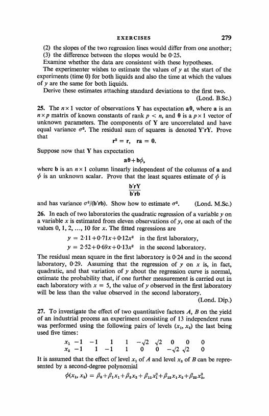
EXERCISES 279
(2) the slopes of the two regression lines would differ from one another;(3) the difference between the slopes would be 0.25.Examine whether the data are consistent with these hypotheses.The experimenter wishes to estimate the values of y at the start of the
experiments (time 0) for both liquids and also the time at which the valuesof y are the same for both liquids.
Derive these estimates attaching standard deviations to the first two.(Lond. B.Sc.)
25. The n x 1 vector of observations Y has expectation a0, where a is ann x p matrix of known constants of rank p < n, and 0 is a p x 1 vector ofunknown parameters. The components of Y are uncorrelated and haveequal variance Q2. The residual sum of squares is denoted Y'rY. Provethat r2=r, ra=0.Suppose now that Y has expectation
aO+b¢,where b is an n x 1 column linearly independent of the columns of a and
is an unknown scalar. Prove that the least squares estimate of 0 is
b'rYb'rb
and has variance 0-2/(b'rb). Show how to estimate 0-2. (Lond. M.Sc.)
26. In each of two laboratories the quadratic regression of a variable y ona variable x is estimated from eleven observations of y, one at each of thevalues 0, 1, 2, ..., 10 for x. The fitted regressions are
y = 2.11+0.71x+0.12x2 in the first laboratory,y = 2.52+0.69x+0.13x2 in the second laboratory.
The residual mean square in the first laboratory is 0.24 and in the secondlaboratory, 0.29. Assuming that the regression of y on x is, in fact,quadratic, and that variation of y about the regression curve is normal,estimate the probability that, if one further measurement is carried out ineach laboratory with x = 5, the value of y observed in the first laboratorywill be less than the value observed in the second laboratory.
(Lond. Dip.)
27. To investigate the effect of two quantitative factors A, B on the yieldof an industrial process an experiment consisting of 13 independent runswas performed using the following pairs of levels (x,, x2) the last beingused five times:
X, -1 -1 1 1 -V2 V2 0 0 0x2 -1 1 -1 1 0 0 - V2 J2 0
It is assumed that the effect of level x, of A and level x2 of B can be repre-sented by a second-degree polynomial
Y'(x1, X2) = No+/31x3+N2x2+Yllx1+fi12x1x2+N22x2,
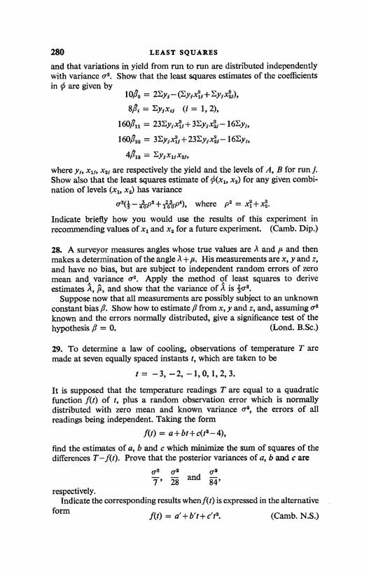
280 LEAST SQUARES
and that variations in yield from run to run are distributed independentlywith variance 0-2. Show that the least squares estimates of the coefficientsin ¢ are given by
10A0 = 2EY,-(Ey,xi,+Ey,x2,),
O, = EY,x, (i = 1, 2),
16011 = 23 Ey, x2,, + 3 EY x2, -16EY,,
16022 = 3Ey xi,+23Ey,x22,-16Ey,,
4A.2 = EY,x1,x2,,
where y,, x1,, x2, are respectively the yield and the levels of A, B for run j.Show also that the least squares estimate of c(x1, x2) for any given combi-nation of levels (x1, x2) has variance
.Q2(5-op2+i6op4), where p2 = xi+X2
Indicate briefly how you would use the results of this experiment inrecommending values of x1 and x2 for a future experiment. (Camb. Dip.)
28. A surveyor measures angles whose true values are A and u and thenmakes a determination of the angle A + p. His measurements are x, y and z,and have no bias, but are subject to independent random errors of zeromean and variance Q2. Apply the method of least squares to deriveestimates A, P, and show that the variance of . is 3Q2.
Suppose now that all measurements are possibly subject to an unknownconstant bias ft. Show how to estimate /3 from x, y and z, and, assuming 0known and the errors normally distributed, give a significance test of thehypothesis /3 = 0. (Lond. B.Sc.)
29. To determine a law of cooling, observations of temperature T aremade at seven equally spaced instants t, which are taken to be
t= -3,-2,-1,0,1,2,3.It is supposed that the temperature readings T are equal to a quadraticfunction f(t) of t, plus a random observation error which is normallydistributed with zero mean and known variance Q2, the errors of allreadings being independent. Taking the form
f(t) = a+bt+c(t2-4),
find the estimates of a, b and c which minimize the sum of squares of thedifferences T-f(t). Prove that the posterior variances of a, b and c are
Q2 a2 U2
7 ' 28and 84,
respectively.Indicate the corresponding results whenf(t) is expressed in the alternative
form f(t) = a'+b't+c't2. (Camb. N.S.)
EXERCISES 281
30. The random variables Y1, ..., Y. have covariance matrix 0-2V, where vis a known positive definite n x n matrix,
-6,(Ya) = Oxi,
where x1, ..., x. are known constants and 0 is an unknown (scalar)parameter. Derive from first principles the least squares estimate, 0, of 0and obtain the variance of 0. Compare this variance with that of the`ordinary' least squares estimate Exz YJExi, when v is the matrix with 1in the diagonal elements and p in all off-diagonal elements.
(Lond. M.Sc).
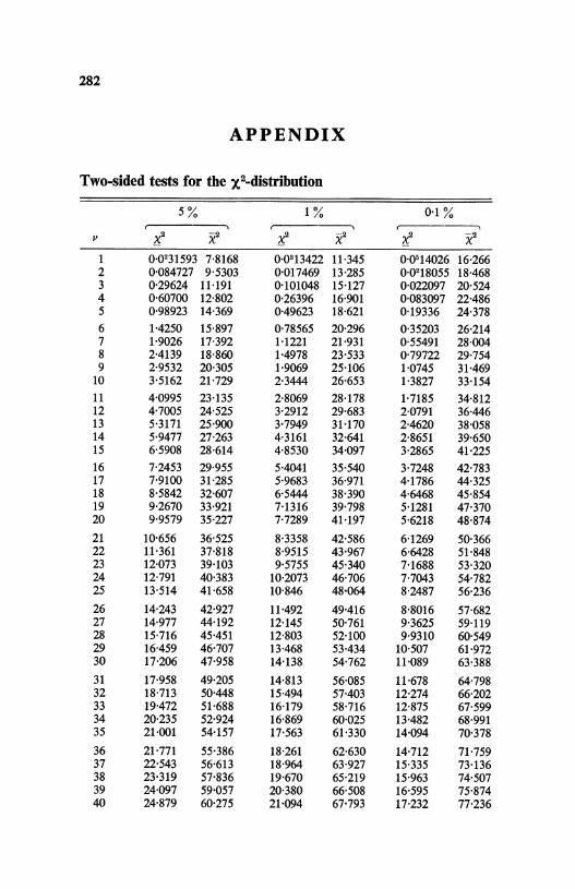
282
APPENDIX
Two-sided tests for the X2-distribution
5% 1% 0.1%
v X2 Z2 x2 Z2x2 x2
1 0.0231593 7.8168 0.0313422 11.345 0.0614026 16.2662 0.084727 9.5303 0.017469 13.285 0.0218055 18.4683 0.29624 11.191 0.101048 15.127 0.022097 20.5244 0.60700 12.802 0.26396 16.901 0.083097 22.4865 0.98923 14.369 0.49623 18.621 0.19336 24.378
6 1.4250 15.897 0.78565 20.296 0.35203 26.2147 1.9026 17.392 1.1221 21.931 0.55491 28.0048 2.4139 18.860 1.4978 23.533 0.79722 29.7549 2.9532 20.305 1.9069 25.106 1.0745 31.469
10 3.5162 21.729 2.3444 26.653 1.3827 33.154
11 4.0995 23.135 2.8069 28.178 1.7185 34.81212 4.7005 24.525 3.2912 29.683 2.0791 36.44613 5.3171 25.900 3.7949 31.170 2.4620 38.05814 5.9477 27.263 4.3161 32.641 2.8651 39.65015 6.5908 28.614 4.8530 34.097 3.2865 41.225
16 7.2453 29.955 5.4041 35.540 3.7248 42.78317 7.9100 31.285 5.9683 36.971 4.1786 44.32518 8.5842 32.607 6.5444 38.390 4.6468 45.85419 9.2670 33.921 7.1316 39.798 5.1281 47.37020 9.9579 35.227 7.7289 41.197 5.6218 48.874
21 10.656 36.525 8.3358 42.586 6.1269 50.36622 11.361 37.818 8.9515 43.967 6.6428 51.84823 12.073 39.103 9.5755 45.340 7.1688 53.32024 12.791 40.383 10.2073 46.706 7.7043 54.78225 13.514 41.658 10.846 48.064 8.2487 56.236
26 14.243 42.927 11.492 49.416 8.8016 57.68227 14.977 44.192 12.145 50.761 9.3625 59.11928 15.716 45.451 12.803 52.100 9.9310 60.54929 16.459 46.707 13.468 53.434 10.507 61.97230 17.206 47.958 14.138 54.762 11.089 63.388
31 17.958 49.205 14.813 56.085 11.678 64.79832 18.713 50.448 15.494 57.403 12.274 66.20233 19.472 51.688 16.179 58.716 12.875 67.59934 20.235 52.924 16.869 60.025 13.482 68.99135 21.001 54.157 17.563 61.330 14.094 70.378
36 21.771 55.386 18.261 62.630 14.712 71.75937 22.543 56.613 18.964 63.927 15.335 73.13638 23.319 57.836 19.670 65.219 15.963 74.50739 24.097 59.057 20.380 66.508 16.595 75.87440 24.879 60.275 21.094 67.793 17.232 77.236
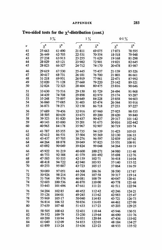
APPENDIX 283
Two-sided tests for the X2-distribution (cont.)5% 1% 0.1
V x2 x2 x2 x x2 x2
41 25.663 61.490 21.811 69.075 17.873 78.59542 26.449 62.703 22.531 70.354 18.518 79.94843 27.238 63.913 23.255 71.629 19.168 81.29844 28.029 65.121 23.982 72.901 19.821 82.64545 28.823 66.327 24.712 74.170 20.478 83.987
46 29.619 67.530 25.445 75.437 21.139 85.32647 30.417 68.731 26.181 76.700 21.803 86.66148 31.218 69.931 26.919 77.961 22.471 87.99249 32.020 71.128 27.660 79.220 23.142 89.32150 32.824 72.323 28.404 80.475 23.816 90.646
51 33.630 73.516 29.150 81.729 24.494 91.96852 34.439 74.708 29.898 82.979 25.174 93.28753 35.248 75.897 30.649 84.228 25.858 94.60354 36.060 77.085 31.403 85.474 26.544 95.91655 36.873 78.271 32.158 86.718 27.233 97.227
56 37.689 79.456 32.916 87.960 27.925 98.53557 38.505 80.639 33.675 89.200 28.620 99.84058 39.323 81.820 34.437 90.437 29.317 101.14259 40.143 83.000 35.201 91.673 30.016 102.44260 40.965 84.178 35.967 92.907 30.719 103.74
61 41.787 85.355 36.735 94.139 31.423 105.0362 42.612 86.531 37.504 95.369 32.130 106.3363 43.437 87.705 38.276 96.597 32.839 107.6264 44.264 88.878 39.049 97.823 33.551 108.9165 45.092 90.049 39.824 99.048 34.264 110.19
66 45.922 91.219 40.600 100.271 34.980 111.4867 46.753 92.388 41.379 101.492 35.698 112.7668 47.585 93.555 42.159 102.71 36.418 114.0469 48.418 94.722 42.940 103.93 37.140 115.3270 49.253 95.887 43.723 105.15 37.864 116.59
71 50.089 97.051 44.508 106.36 38.590 117.8772 50.926 98.214 45.294 107.58 39.317 119.1473 51.764 99.376 46.081 108.79 40.047 120.4174 52.603 100.536 46.870 110.00 40.778 121.6875 53.443 101.696 47.661 111.21 41.511 122.94
76 54.284 102.85 48.452 112.42 42.246 124.2177 55.126 104.01 49.245 113.62 42.983 125.4778 55.969 105.17 50.040 114.83 43.721 126.7379 56.814 106.32 50.836 116.03 44.461 127.9980 57.659 107.48 51.633 117.23 45.203 129.25
81 58.505 108.63 52.431 118.44 45.946 130.5182 59.352 109.79 53.230 119.64 46.690 131.7683 60.200 110.94 54.031 120.84 47.436 133.0284 61.049 112.09 54.833 122.03 48.184 134.2785 61.899 113.24 55.636 123.23 48.933 135.52
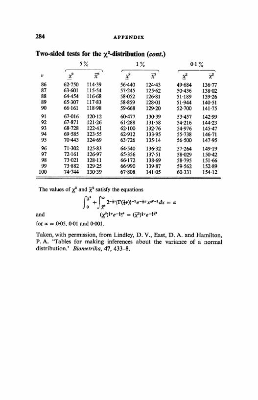
284 APPENDIX
Two-sided tests for the X2-distribution (cont.)5/ 1/ 0.1%
I' x2 x2 x2 z2 _ z2
86 62.750 114.39 56.440 124.43 49.684 136.7787 63.601 115.54 57.245 125.62 50.436 138.0288 64.454 116.68 58.052 126.81 51.189 139.2689 65.307 117.83 58.859 128.01 51.944 140.5190 66.161 118.98 59.668 129.20 52.700 141.75
91 67.016 120.12 60.477 130.39 53.457 142.9992 67.871 121.26 61.288 131.58 54.216 144.2393 68.728 122.41 62.100 132.76 54.976 145.4794 69.585 123.55 62.912 133.95 55.738 146.7195 70.443 124.69 63.726 135.14 56.500 147.95
96 71.302 125.83 64.540 136.32 57.264 149.1997 72.161 126.97 65.356 137.51 58.029 150.4298 73.021 128.11 66.172 138.69 58.795 151.6699 73.882 129.25 66.990 139.87 59.562 152.89
100 74.744 130.39 67.808 141.05 60.331 154.12
The values of x2 and X2 satisfy the equations
x°+fO
U x'
and (x2)i"e-ix' = (x2)i"e-ix
for a = 0.05, 0.01 and 0.001.
Taken, with permission, from Lindley, D. V., East, D. A. and Hamilton,P. A. 'Tables for making inferences about the variance of a normaldistribution.' Biometrika, 47, 433-8.
285
BIBLIOGRAPHY
ALEXANDER, H. W. (1961). Elements of Mathematical Statistics. NewYork: John Wiley and Sons Inc.
BIRNBAUM, Z. W. (1962). Introduction to Probability and MathematicalStatistics. New York: Harper and Bros.
BLACKWELL, D. and GIRSHICK, M. A. (1954). Theory of Games andStatistical Decisions. New York: John Wiley and Sons Inc.
BRUNK, H. D. (1960). An Introduction to Mathematical Statistics. Boston:Ginn and Co. Ltd.
CHERNOFF, H. and MOSES, L. E. (1959). Elementary Decision Theory. NewYork: John Wiley and Sons Inc.
COCHRAN, W. G. (1963). Sampling Techniques. New York: John Wileyand Sons Inc.
COCHRAN, W. G. and Cox, G. M. (1957). Experimental Designs. NewYork: John Wiley and Sons Inc.
Cox, D. R. (1958). Planning of Experiments. New York: John Wiley andSons Inc.
CRAMER, H. (1946). Mathematical Methods of Statistics. PrincetonUniversity Press.
DAVID, F. N. (1954). Tables of the Ordinates and Probability Integral of theDistribution of the Correlation Coefficient in Small Samples. CambridgeUniversity Press.
DAVIES, O. L. (editor) (1957). Statistical Methods in Research and Produc-tion, 3rd edition. Edinburgh: Oliver and Boyd.
DAVIS, H. T. (1933). Tables of the Higher Mathematical Functions, volume I.Bloomington: Principia Press.
FISHER, R. A. (1958). Statistical Methods for Research Workers, 13thedition. Edinburgh: Oliver and Boyd.
FISHER, R. A. (1959). Statistical Methods and Scientific Inference, 2ndedition. Edinburgh: Oliver and Boyd.
FISHER, R. A. (1960). The Design of Experiments, 7th edition. Edinburgh:Oliver and Boyd.
FISHER, R. A. and YATES, F. (1963). Statistical Tables for Biological,Agricultural and Medical Research, 6th edition. Edinburgh: Oliver andBoyd.
FRASER, D. A. S. (1958). Statistics: an Introduction. New York: JohnWiley and Sons Inc.
GREENWOOD, J. A. and HARTLEY, H. O. (1962). Guide to Tables in Mathe-matical Statistics. Princeton University Press.
HoEL, P. G. (1960). Introduction to Mathematical Statistics, 2nd edition.New York: John Wiley and Sons Inc.
HOGG, R. V. and CRAIG, A. T. (1959). Introduction to MathematicalStatistics. New York: Macmillan.
286 BIBLIOGRAPHY
JEFFREYS, H. (1961). Theory of Probability, 3rd edition. Oxford:Clarendon Press.
KEMPTHORNE, O. (1952). The Design and Analysis of Experiments. NewYork: John Wiley and Sons Inc.
KENDALL, M. G. and STUART, A. (1958, 1961). The Advanced Theory ofStatistics. Two volumes. London: Griffin and Co.
LINDLEY, D. V. and MILLER, J. C. P. (1961). Cambridge ElementaryStatistical Tables. Cambridge University Press.
PEARSON, E. S. and HARTLEY, H. O. (1958). Biometrika Tables forStatisticians, volume I. Cambridge University Press.
PLACKETT, R. L. (1960). Principles of Regression Analysis. Oxford:Clarendon Press.
RAIFFA, H. and SCHLAIFER, R. (1961). Applied Statistical Decision Theory.Boston: Harvard University Graduate School of Business Administra-tion.
SCHEFFE, H. (1959). The Analysis of Variance. New York: John Wiley andSons Inc.
SCHLAIFER, R. (1959). Probability and Statistics for Business Decisions.New York: McGraw-Hill Book Co. Inc.
TUCKER, H. G. (1962). An Introduction to Probability and MathematicalStatistics. New York: Academic Press.
WEISS, L. (1961). Statistical Decision Theory. New York: McGraw-HillBook Co. Inc.
WILKS, S. S. (1962). Mathematical Statistics. New York: John Wiley andSons Inc.
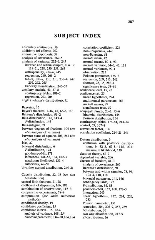
287
SUBJECT INDEX
absolutely continuous, 56additivity (of effects), 252alternative hypothesis, 59analysis of covariance, 262-5analysis of variance, 232-6, 245
between and within samples, 104-12,119-21, 228, 250, 253, 265
orthogonality, 234-6, 245regression, 210, 261-2tables, 105-7, 110, 210, 233-4, 247,
256, 262, 265two-way classification, 246-57
ancillary statistic, 49, 57-8contingency tables, 181-2regression, 203, 205
angle (Behrens's distribution), 91
Bayesian, 15Bayes's theorem, 1-16, 47, 65-6, 116Behrens's distribution, 91-2Beta-distribution, 141, 143-4
F-distribution, 146Beta-integral, 39between degrees of freedom, 104 (see
also analysis of variance)between sums of squares 104, 261 (see
also analysis of variance)bias, 27
binomial distribution, 6F-distribution, 124goodness-of-fit, 171inferences, 141-53, 164, 182-3maximum likelihood, 133-4sufficiency, 49-50
bivariate normal distribution, 214-21
Cauchy distribution, 22, 38 (see alsot-distribution)
central limit theorem, 21, 28coefficient of dispersion, 166, 183combination of observations, 112-21comparative experiments, 78-9computation (see under numerical
methods)conditional density, 19confidence coefficient, 15confidence interval, 15, 22-6
analysis of variance, 108, 254binomial parameter, 146-50,164,184
correlation coefficient, 221non-uniqueness, 24-5non-Bayesian, 68normal mean, 42normal means, 80-1, 93normal variance, 34-6, 43, 111normal variances, 90-1observation, 213Poisson parameter, 155-7regression, 209, 213, 246shortest, 25, 35, 282-4significance tests, 58-61
confidence level, 15, 23confidence set, 25
linear hypotheses, 224multinomial parameters, 164normal means, 97significance tests, 59
conjugate family, 20-1, 55-6binomial distribution, 145Poisson distribution, 154
contingency tables, 176-84, 213-14control, 79, 107-8correction factor, 106correlation coefficient, 214-21, 246
Datum distribution, 9confusion with posterior distribu-
tion, 9, 32-3, 67-8, 115, 231:maximum likelihood, 139
decision theory, 62-7dependent variable, 206degrees of freedom, 81-3
analysis of covariance, 265Behrens's distribution, 91between and within samples, 78, 96,
103-4, 110, 118binomial parameter, 141, 146contingency table, 177F-distribution, 86, 88goodness-of-fit, 157, 168, 172-3interaction, 249linear hypothesis, 222, 224, 226,
233Poisson parameter, 153regression, 204, 208-9, 257, 259t-distribution, 36two-way classification, 247-9x2-distribution, 26
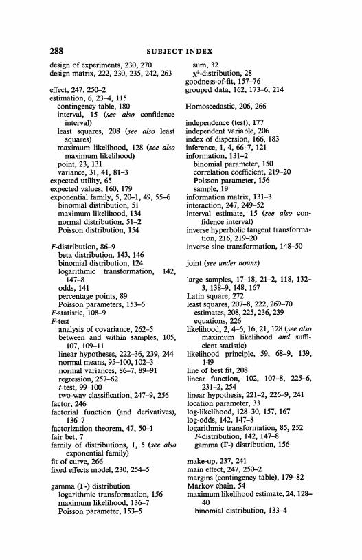
288 SUBJECT
design of experiments, 230, 270design matrix, 222, 230, 235, 242, 263
effect, 247, 250-2estimation, 6, 23-4, 115
contingency table, 180interval, 15 (see also confidence
interval)least squares, 208 (see also least
squares)maximum likelihood, 128 (see also
maximum likelihood)point, 23, 131variance, 31, 41, 81-3
expected utility, 65expected values, 160, 179exponential family, 5, 20-1, 49, 55-6
binomial distribution, 51maximum likelihood, 134normal distribution, 51-2Poisson distribution, 154
F-distribution, 86-9beta distribution, 143, 146binomial distribution, 124logarithmic transformation, 142,
147-8odds, 141percentage points, 89Poisson parameters, 153-6
F-statistic, 108-9F-test
analysis of covariance, 262-5between and within samples, 105,
107, 109-11linear hypotheses, 222-36, 239, 244normal means, 95-100, 102-3normal variances, 86-7, 89-91regression, 257-62t-test, 99-100two-way classification, 247-9, 256
factor, 246factorial function (and derivatives),
136-7factorization theorem, 47, 50-1fair bet, 7family of distributions, 1, 5 (see also
exponential family)fit of curve, 266fixed effects model, 230, 254-5
gamma (r-) distributionlogarithmic transformation, 156maximum likelihood, 136-7Poisson parameter, 153-5
INDEX
sum, 32x'-distribution, 28
goodness-of-fit, 157-76grouped data, 162, 173-6, 214
Homoscedastic, 206, 266
independence (test), 177independent variable, 206index of dispersion, 166, 183inference, 1, 4, 66-7, 121information, 131-2
binomial parameter, 150correlation coefficient, 219-20Poisson parameter, 156sample, 19
information matrix, 131-3interaction, 247, 249-52interval estimate, 15 (see also con-
fidence interval)inverse hyperbolic tangent transforma-
tion, 216, 219-20inverse sine transformation, 148-50
joint (see under nouns)
large samples, 17-18, 21-2, 118, 132-3, 138-9, 148, 167
Latin square, 272least squares, 207-8, 222, 269-70
estimates, 208, 225, 236, 239equations, 226
likelihood, 2, 4-6, 16, 21, 128 (see alsomaximum likelihood and suffi-cient statistic)
likelihood principle, 59, 68-9, 139,149
line of best fit, 208linear function, 102, 107-8, 225-6,
231-2, 254linear hypothesis, 221-2, 226-9, 241location parameter, 33log-likelihood, 128-30, 157, 167log-odds, 142, 147-8logarithmic transformation, 85, 252
F-distribution, 142, 147-8gamma (r-) distribution, 156
make-up, 237, 241main effect, 247, 250-2margins (contingency table), 179-82Markov chain, 54maximum likelihood estimate, 24, 128-
40binomial distribution, 133-4
SUBJECT INDEX
maximum likelihood estimate (cont.)exponential family, 134gamma (F-) distribution, 136-7goodness-of-fit, 170-1least squares, 208normal distribution, 132-3sampling distribution, 139
maximum likelihood equation, 134-7
mean (see under normal distribution)mean square, 78, 105minimal sufficient statistic, 52-3mistakes, 13mixed model, 254-5multinomial distribution, 161, 181
Poisson distribution, 165-6multiple regression, 241-6
on powers, 266-9multiple regression coefficient, 241,
245-6multiplication law of probabilities, 4multivariate normal distribution (see
also bivariate)likelihood, 114-15, 118-21posterior distribution of means, 223,
225,230-1,245-6regression transformation, 223, 231,
237sufficient statistics, 74
Newton's method, 134-6non-Bayesian methods, 25-6, 67-70,
94-5, 230 (see also datum distribu-tion)
non-orthogonal, 244, 267normal distribution (see also bivariate
and multivariate)exponential family, 51-2maximum likelihood, 132-3mean, 1-23mean and variance, 36-46means, 76-86, 91-104, 227-8sufficient statistics, 51-2variance, 26-36, 101, 111-12variances, 86-91
nuisance parameter, 38, 57-8, 232null hypothesis, 59, 67, 232numerical methods
between and within samples, 106-7linear hypothesis, 236-46maximum likelihood, 134-6two-way classification, 253
observed values, 160, 179odds, 7, 141, 146
289
ordinates (regression), 259-61orthogonal design, 119, 234-5, 245,
270two-way classification, 252-3
orthogonal polynomials, 267-9
paired comparisons, 83-6parameter, 1, 5 (see also nuisance
parameter)Pareto distribution, 73percentage points, 34
F-distribution, 88-9t-distribution, 39
x2-distribution, 34-5
point estimate (see under estimation)Poisson distribution, 153-7
goodness-of-fit, 173means, 165-6multinomial distribution, 166
Poisson process, 137polynomial regression, 266-9posterior distribution, 2, 21-2, 121 (see
also datum distribution, and largesamples)
approximation by maximum likeli-hood, 129-32, 138
binomial distribution, 141-8conjugate distribution, 55-6correlation coefficient, 214-15, 220-
1
decision theory, 65goodness-of-fit, 157-60linear function, 102, 107-8, 225-6,
231-2,254linear hypothesis, 223-6, 230multivariate normal, 114-15normal mean, 2-3, 7-11, 13-16,
36-7, 41-2, 101normal mean and variance, 44-5,
133normal means, 76-83, 91-3, 95-9,
103,112-14,119-21normal variances, 86-7, 89-91Poisson distribution, 153-4prior to next sample, 116regression, 204-5, 207, 245-6:
conditional expectation, 211 line,211-12
sufficiency, 46-7tabulation, 45-6, 83
precision, 8, 10, 24, 30-1, 116-18prediction, 11-12, 66
regression, 212-13
principle of precise measurement,12
290 SUBJECT INDEX
prior distribution, 2, 7, 16-17, 21, 132
(see also large samples)between and within samples, 112,
119-21binomial distribution, 141conjugate distribution, 55-6correlation coefficient, 218-20decision theory, 65goodness-of-fit, 163, 166-7, 176linear hypothesis, 229maximum likelihood, 132normal mean, 2-3, 7normal mean and variance, 40normal variance, 26-33Poisson distribution, 153posterior of last sample, 116regression, 205-6sample information, 20-1, 151-3significance test, 61-2uniform, 18-19, 33, 145, 155,
220vague prior, 9, 13-18, 31-3, 76, 132,
144-6, 155, 219-20probability distribution (derivation),
97-8, 103-4probable error, 23product (vectors), 236
random effects model, 254-5random sample, 1-4, 10random sampling numbers, 53random sequence of trials, 141-53,
157, 168, 176-8range, 56reduction of data, 10reduction in sums of squares, 222-5,
232-6, 238, 245analysis of covariance, 262-5regression, 258-60
regression, 203analysis of covariance, 265coefficient, 207, 241, 245-6linear, 203-14, 217, 228-9, 257-
62multiple, 241-6polynomial, 266-9reduction, 264-5
replication, 247, 255residual sum of squares, 222, 233-4,
238, 243-5analysis of covariance, 262-3regression, 209, 258, 260-2two-way classification, 247-8, 253,
256robustness, 13
sample beliefs, 11-12, 66regression, 211-13
sample correlation coefficient, 218sample information, 19-20sample mean, 41sample regression coefficient, 207, 245-
6sample variance, 41sampling, 4, 270Sheppard's correction, 163, 175-6significance level, 59
exact, 60significance tests, 58-62, 111, 163 (see
also F-, t- and x2-tests)non-Bayesian, 67-70, 94-5
square root transformation, 156standard deviation, 8standard error, 23statistic, 46Stirling's formula, 137sufficiency, 10, 30, 41, 46-58sufficiency principle, 46sufficient statistic, 23, 46-58, 67
between and within samples, 103binomial distribution, 49-51, 141correlation coefficient, 218linear hypothesis, 236maximum likelihood, 134normal distribution, 51-2Poisson distribution, 153regression, 210
sum of squares, 78, 81-2 (see alsomean square, reduction in sum ofsquares, residual, between, totaland within sum of squares)
uncorrected, 82sum of squares due to regression,
209
t-distribution, 36-9Behrens's distribution, 93-4F-distribution, 88normal distribution, 41-2
t-testF-test, 99-100linear functions, 102, 107-8, 225-6,
231-2, 254normal mean, 42normal means, 79-86, 99-101regression, 203-5, 208-10
tests of hypotheses, 24 (see also signi-ficance tests)
total degrees of freedom, 104total sum of squares, 104, 232-6,
261
SUBJECT INDEX
transformation to constant informationbinomial distribution, 149-50correlation coefficient, 219-20Poisson distribution, 156
triangular matrix, 237two-way classification, 246-57
uncorrected sum of squares, 106uniform distribution (see also prior
distribution)goodness-of-fit, 163maximum likelihood, 140sufficiency, 56
utility, 64utility function, 64
vague prior knowledge, 9, 13-18, 76binomial distribution, 31-3maximum likelihood, 132normal variance, 31-3Poisson distribution, 155
variance (see also normal distribution)assumption of equality, 80-2, 92, 99,
105, 112, 118, 227; homoscedastic,206, 266
ratio, 90
291
weighing example, 119, 228weight, 113weighted least squares, 269-70weighted mean, 8, 31, 113within degrees of freedom, 78, 104 (see
also analysis of variance)within sum of squares, 78, 82, 104,
117-18, 261 (see also analysis ofvariance)
x2-distribution, 26-30
F-distribution, 88gamma (r-) distribution, 28percentage points, 34, 282-4
x2-statistic, 160
x'2-statistic, 167x2-test
binomial distribution, 164, 182-3contingency tables, 176, 178goodness-of-fit, 160, 168linear hypothesis, 225normal variance,26-38, 43,101,111-
12Poisson distribution, 153,155,165-6regression, 204, 209
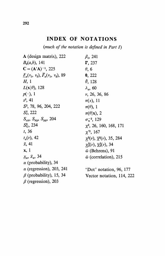
292
INDEX OF NOTATIONS(much of the notation is defined in Part I)
A (design matrix), 222B0(a,b), 141
C = (A'A)-1, 225
Fa(vl, v2), Fa(vl, v2), 89H, 1L(xlO), 128
A.), 1s2, 2,41
S2, 78, 96, 204, 222
ST, 222
S. S., Svy, 204S2;, 234
t, 36
ta(v), 42
x, 41x, 1
xa, J 34
a (probability), 34a (regression), 203, 241
(probability), 15, 34Q (regression), 203
ftf 241r, 2370, 60, 222
0,128AL,, 60
v, 26, 36, 86
IT(x), 11
if(0), 1
7r(0 x), 2
O'n2, 129
x2, 26, 160, 168, 171
x'2, 167
x2(v), x2(v), 35, 284
xa(v), X2 0, 34
Co (Behrens), 91
Co (correlation), 215
`Dot' notation, 96, 177Vector notation, 114, 222