1

Introduction to probability and statistics (1)

Andreas Hoecker (CERN)CERN Summer Student Lecture, 18–21 July 2016

2

Outline (4 lectures)

1st lecture:• Introduction • Probability

2nd lecture:• Probability axioms and hypothesis testing• Parameter estimation• Confidence levels

3rd lecture:• Maximum likelihood fits• Monte Carlo methods• Data unfolding

4th lecture:• Multivariate techniques and machine learning

Acknowledgements and some further reading

• I am particularly grateful to Helge Voss, whose comprehensive statistics lectures serve as model for the present lectures. His latest lectures on multivariate analysis and neural networks at the School of Statistics, 2016: https://indico.in2p3.fr/event/12667/other-view?view=standard

• Glen Cowan’s book “Statistical data analysis” represents a great introduction: http://www.pp.rhul.ac.uk/~cowan/sda

• PDG reviews by G. Cowan on probability (http://pdg.lbl.gov/2013/reviews/rpp2013-rev-probability.pdf ) and statistics (http://pdg.lbl.gov/2013/reviews/rpp2013-rev-statistics.pdf) :

• Luca Lista’s lectures “Practical Statistics for Particle Physicists”, at the CERN-JINR school 2016: https://indico.cern.ch/event/467465/other-view?daysPerRow=5&view=nicecompact

• Kyle Cranmer’s article “Practical Statistics for the LHC”, arXiv:1503.07622

• Harrisson Prospers 2015 CERN Academic Training lecture “Practical Statistics for LHC Physicists”: https://indico.cern.ch/event/358542/

• Machine learning introduction: T. Hastie, R. Tibshirani, J. Friedman, “The Elements of Statistical Learning”, Springer 2001; C.M. Bishop, “Pattern Recognition and Machine Learning”, Springer 2006

• Very incomplete list. Some more references are given throughout the lecture.

3

Why we need probability in the particle world

4

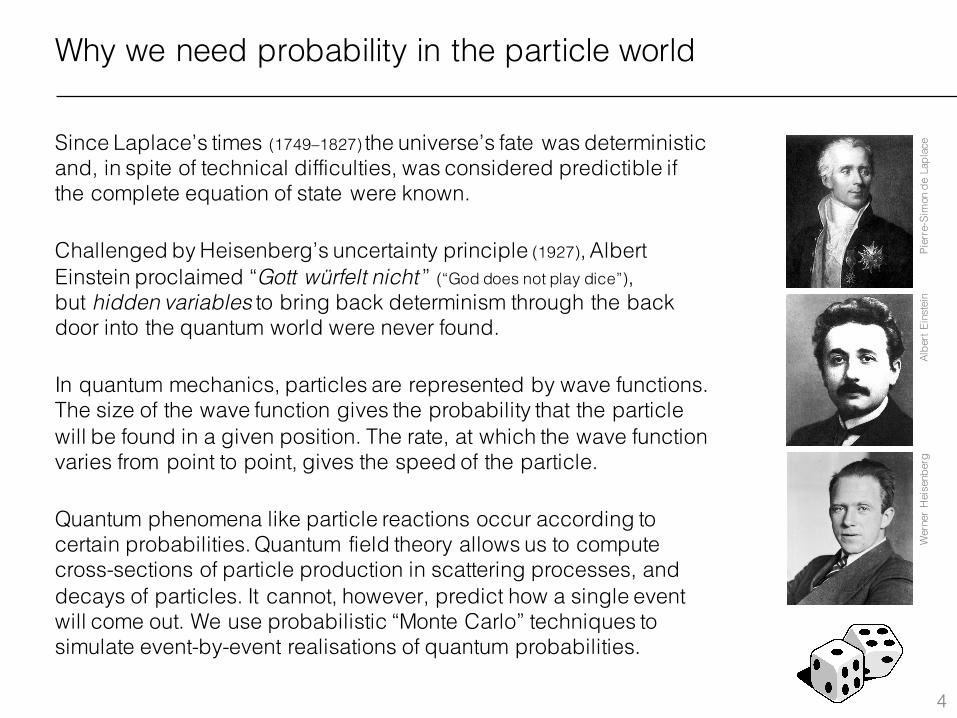
Since Laplace’s times (1749–1827) the universe’s fate was deterministic and, in spite of technical difficulties, was considered predictible if the complete equation of state were known.

Challenged by Heisenberg’s uncertainty principle (1927), Albert Einstein proclaimed “Gott würfelt nicht ” (“God does not play dice”), but hidden variables to bring back determinism through the back door into the quantum world were never found.

In quantum mechanics, particles are represented by wave functions. The size of the wave function gives the probability that the particle will be found in a given position. The rate, at which the wave function varies from point to point, gives the speed of the particle.

Quantum phenomena like particle reactions occur according to certain probabilities. Quantum field theory allows us to compute cross-sections of particle production in scattering processes, and decays of particles. It cannot, however, predict how a single event will come out. We use probabilistic “Monte Carlo” techniques to simulate event-by-event realisations of quantum probabilities.

Pier

re-S

imon

de

Lapl

ace

Albe

rt Ei

nste

inW

erne

r H

eise

nber

g

Statistics of large systems

5

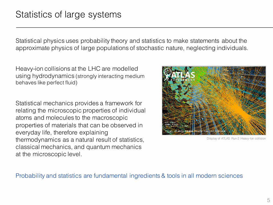
Statistical physics uses probability theory and statistics to make statements about the approximate physics of large populations of stochastic nature, neglecting individuals.

Heavy-ion collisions at the LHC are modelled using hydrodynamics (strongly interacting medium behaves like perfect fluid)

Statistical mechanics provides a framework for relating the microscopic properties of individual atoms and molecules to the macroscopic properties of materials that can be observed in everyday life, therefore explaining thermodynamics as a natural result of statistics, classical mechanics, and quantum mechanics at the microscopic level.

Display of ATLAS Run-2 Heavy-Ion collision

Probability and statistics are fundamental ingredients & tools in all modern sciences

Statistics in measurement processes

6

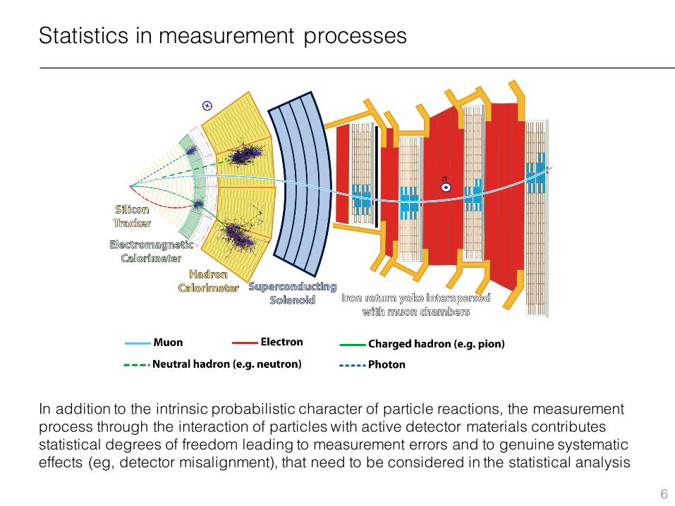
In addition to the intrinsic probabilistic character of particle reactions, the measurement process through the interaction of particles with active detector materials contributes statistical degrees of freedom leading to measurement errors and to genuine systematic effects (eg, detector misalignment), that need to be considered in the statistical analysis

Measurements and hypothesis testing

7

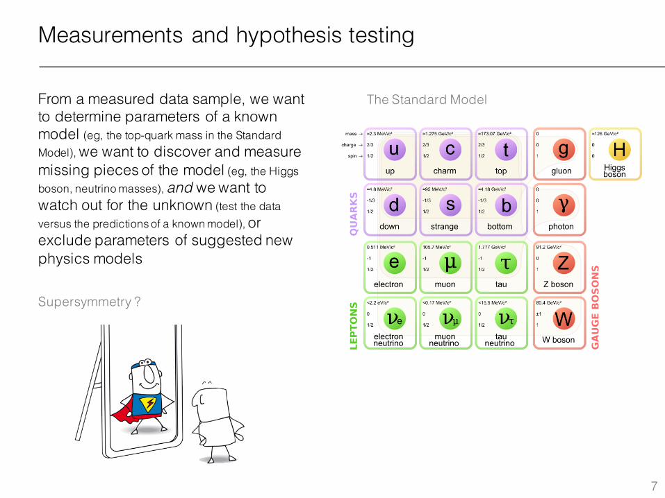
From a measured data sample, we want to determine parameters of a known model (eg, the top-quark mass in the Standard Model), we want to discover and measure missing pieces of the model (eg, the Higgs boson, neutrino masses), and we want to watch out for the unknown (test the data versus the predictions of a known model), or exclude parameters of suggested new physics models

The Standard Model

Supersymmetry ?

Ingredients

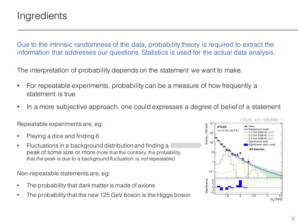
Due to the intrinsic randomness of the data, probability theory is required to extract the information that addresses our questions. Statistics is used for the actual data analysis.

The interpretation of probability depends on the statement we want to make.

• For repeatable experiments, probability can be a measure of how frequently a statement is true

• In a more subjective approach, one could expresses a degree of belief of a statement

8

1.5 2 2.5 3 3.5

Even

ts /

100

GeV

1−10

1

10

210

310

410DataBackground model1.5 TeV EGM W', c = 12.0 TeV EGM W', c = 12.5 TeV EGM W', c = 1Significance (stat)Significance (stat + syst)

ATLAS-1 = 8 TeV, 20.3 fbs

WZ Selection

[TeV]jjm1.5 2 2.5 3 3.5

Sign

ifica

nce

2−1−0123

Repeatable experiments are, eg:

• Playing a dice and finding 6• Fluctuations in a background distribution and finding a

peak of some size or more (note that the contrary: the probability that the peak is due to a background fluctuation, is not repeatable)

Non-repeatable statements are, eg:

• The probability that dark matter is made of axions• The probability that the new 125 GeV boson is the Higgs boson

[ ATLAS, arXiv:1506.00962 ]

Statistical distributions

Measurement results typically follow some “distribution”, ie, the data do not appear at fixed values, but are “spread out” in a characteristic way

Which type of distribution it follows depends on the particular case

• It is important to know the occurring distributions to be able to pick the correct one when interpreting the data (example: Poisson vs. Compound Poisson)

• …and it is important to know their characteristics to extract the correct information

Note: in statistical context, instead of “data” that follow a distribution, one often (typically) speaks of a “random variable”

9

Probability distribution / density of a random variable

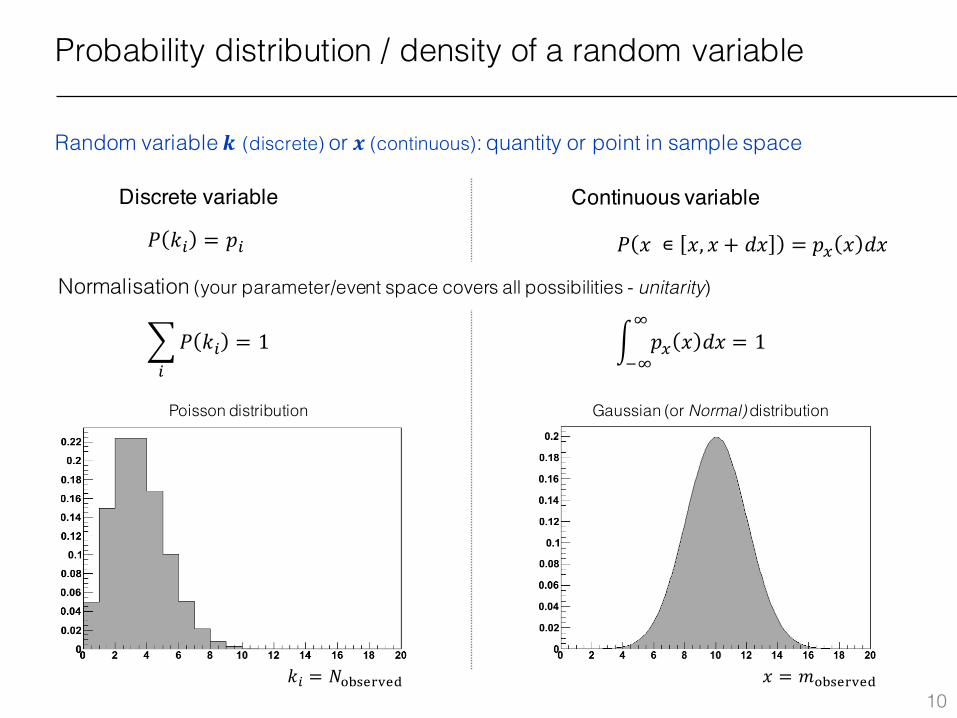
Random variable 𝒌 (discrete) or 𝒙 (continuous): quantity or point in sample space

10

Discrete variable Continuous variable

𝑃 𝑘% = 𝑝% 𝑃 𝑥 ∊ 𝑥, 𝑥 + 𝑑𝑥 = 𝑝. 𝑥 𝑑𝑥

/ 𝑝. 𝑥 𝑑𝑥0

10= 13𝑃 𝑘%

%

= 1

Normalisation (your parameter/event space covers all possibilities - unitarity)

𝑘% = 𝑁56789:8; 𝑥 = 𝑚56789:8;

Poisson distribution Gaussian (or Normal) distribution

Cumulative distribution

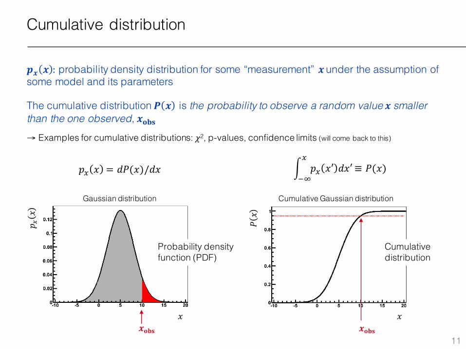
𝒑𝒙 𝒙 : probability density distribution for some “measurement” 𝒙 under the assumption of some model and its parameters

The cumulative distribution 𝑷 𝒙 is the probability to observe a random value 𝒙 smaller than the one observed, 𝒙𝐨𝐛𝐬→ Examples for cumulative distributions: 𝜒2, p-values, confidence limits (will come back to this)

11

Probability density function (PDF)

Cumulative distribution

/ 𝑝. 𝑥′ 𝑑𝑥′.

10≡ 𝑃(𝑥)𝑝. 𝑥 = 𝑑𝑃(𝑥)/𝑑𝑥

𝒙𝐨𝐛𝐬

𝑝 .𝑥

Gaussian distribution Cumulative Gaussian distribution

𝒙𝐨𝐛𝐬

𝑃𝑥

𝑥 𝑥

Selected probability (density) distributions

12

Imagine a monkey discovered a huge bag of alphabet noodles. She blindly draws noodles out of the bag and places them in a row before her. The text reads: “TO BE OR NOT TO BE”

The probability for this to happen is about 10–22

Infinite monkey theorem: provided enough time, the monkey will type Shakespeare's Hamlet

Bernoulli distribution

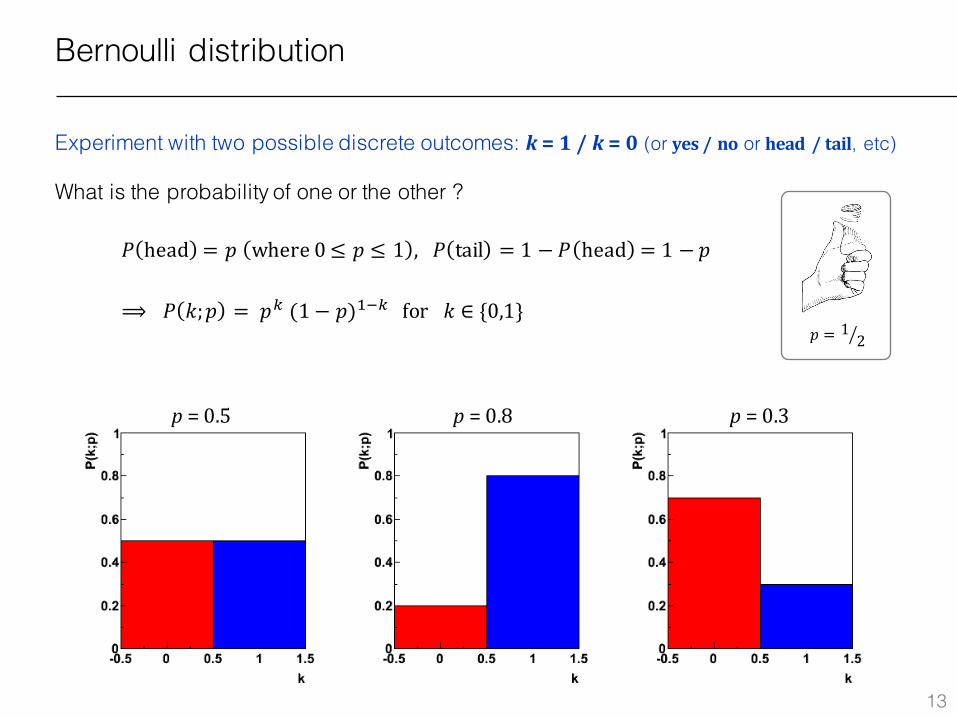
Experiment with two possible discrete outcomes: k =1/ k =0 (or yes/no or head /tail, etc)

What is the probability of one or the other ?

13

⟹ 𝑃 𝑘;𝑝 = 𝑝J (1 − 𝑝)L1Jfor𝑘 ∈ {0,1}𝑝 = 1

2U

p =0.5 p=0.8 p=0.3

𝑃 head = 𝑝 where0 ≤ 𝑝 ≤ 1 , 𝑃 tail = 1 − 𝑃 head = 1 − 𝑝

Binomial distribution (very important!)

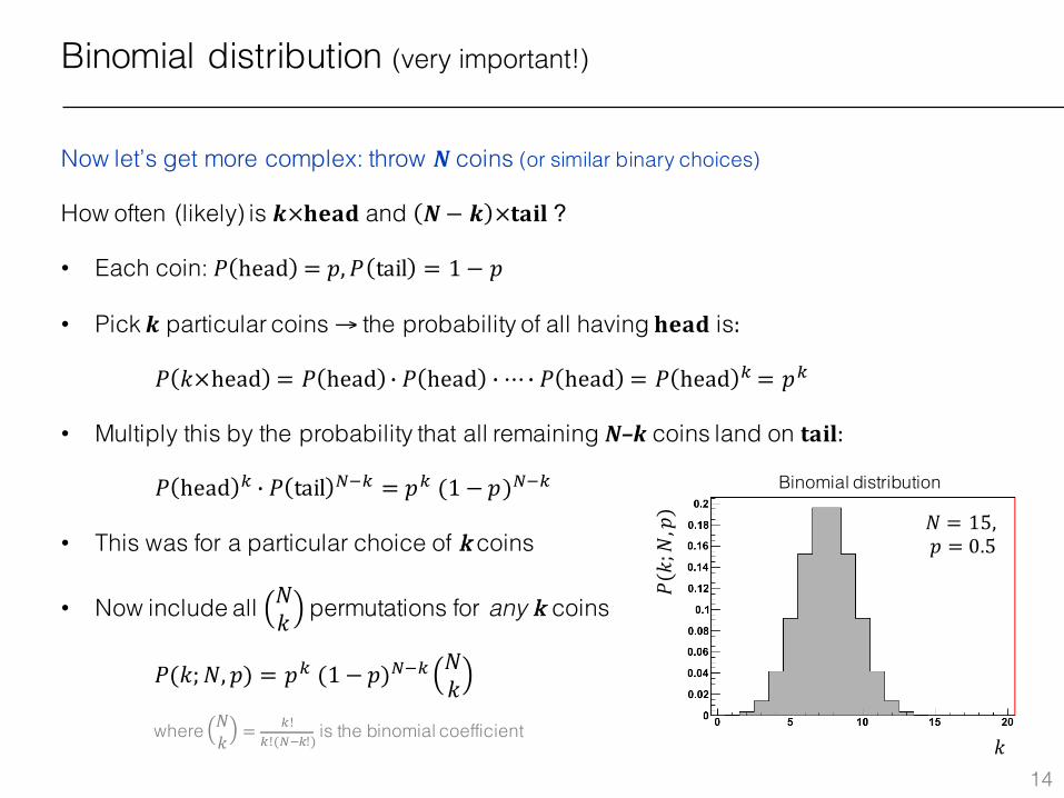
Now let’s get more complex: throw N coins (or similar binary choices)

How often (likely) is 𝒌×𝐡𝐞𝐚𝐝 and 𝑵− 𝒌 ×𝐭𝐚𝐢𝐥 ?

• Each coin: 𝑃 head = 𝑝, 𝑃 tail = 1 − 𝑝

• Pick 𝒌 particular coins → the probability of all having 𝐡𝐞𝐚𝐝 is:

• Multiply this by the probability that all remaining N–k coins land on 𝐭𝐚𝐢𝐥:

• This was for a particular choice of k coins

• Now include all 𝑁𝑘 permutations for any k coins

14

𝑃 𝑘×head = 𝑃 head j 𝑃 head j ⋯ j 𝑃 head = 𝑃 head J = 𝑝J

𝑃 head J j 𝑃 tail l1J = 𝑝J (1 − 𝑝)l1J

𝑃(𝑘; 𝑁, 𝑝) = 𝑝J (1 − 𝑝)l1J 𝑁𝑘

where 𝑁𝑘 = J!J!(l1J!) is the binomial coefficient

𝑃(𝑘;𝑁,𝑝)

𝑘

𝑁 = 15,𝑝 = 0.5

Binomial distribution

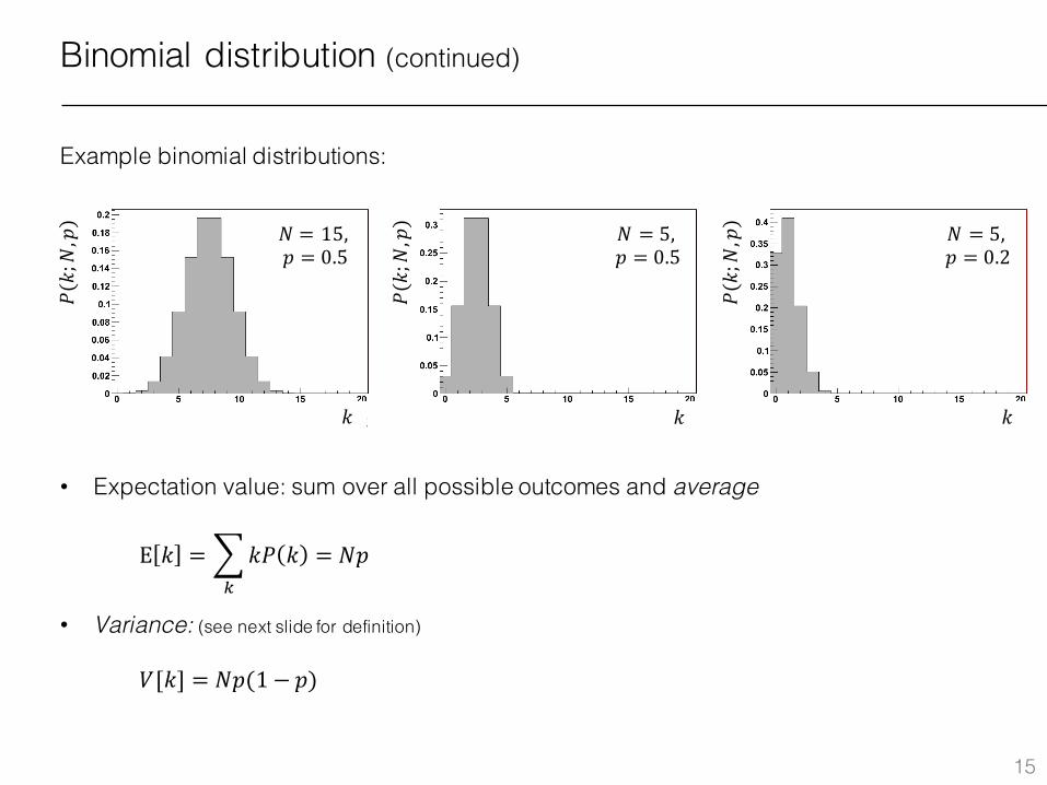
Binomial distribution (continued)

Example binomial distributions:

15

• Expectation value: sum over all possible outcomes and average

• Variance: (see next slide for definition)

E 𝑘 = 3𝑘𝑃 𝑘J

= 𝑁𝑝

𝑉[𝑘] = 𝑁𝑝(1 − 𝑝)

𝑘 𝑘𝑘

𝑃(𝑘;𝑁,𝑝)

𝑃(𝑘;𝑁,𝑝)

𝑃(𝑘;𝑁,𝑝)𝑁 = 15,

𝑝 = 0.5𝑁 = 5,𝑝 = 0.5

𝑁 = 5,𝑝 = 0.2

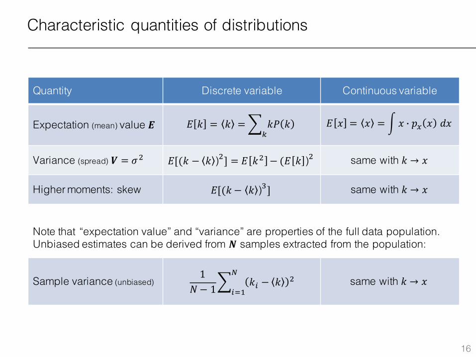
Characteristic quantities of distributions

16

Quantity Discrete variable Continuous variable

Expectation (mean) value 𝑬 𝐸 𝑘 = 𝑘 =3 𝑘𝑃 𝑘J

𝐸 𝑥 = 𝑥 = / 𝑥 j 𝑝. 𝑥 𝑑𝑥

Variance (spread) 𝑽 = 𝜎x 𝐸[(𝑘 − 𝑘 )x] = 𝐸 𝑘x − (𝐸 𝑘 )x same with 𝑘 → 𝑥

Higher moments: skew 𝐸[(𝑘 − 𝑘 )z] same with 𝑘 → 𝑥

Note that “expectation value” and “variance” are properties of the full data population.Unbiased estimates can be derived from 𝑵 samples extracted from the population:

Sample variance (unbiased)1

𝑁− 13 𝑘% − 𝑘 x

l

%{Lsame with 𝑘 → 𝑥

Characteristic quantities of distributions (continued)

17

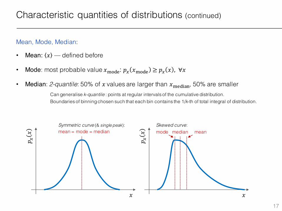
Mean, Mode, Median:

• Mean: 𝑥 — defined before

• Mode: most probable value 𝑥|5;8: 𝑝. 𝑥|5;8 ≥ 𝑝. 𝑥 , ∀𝑥

• Median: 2-quantile: 50% of 𝑥values are larger than 𝑥|8;���, 50% are smallerCan generalise k-quantile : points at regular intervals of the cumulative distribution.Boundaries of binning chosen such that each bin contains the 1/k-th of total integral of distribution.

mean = mode = medianSkewed curve:mode median mean

Symmetric curve (& single peak):

𝑥 𝑥

𝑝 .𝑥

𝑝 .𝑥

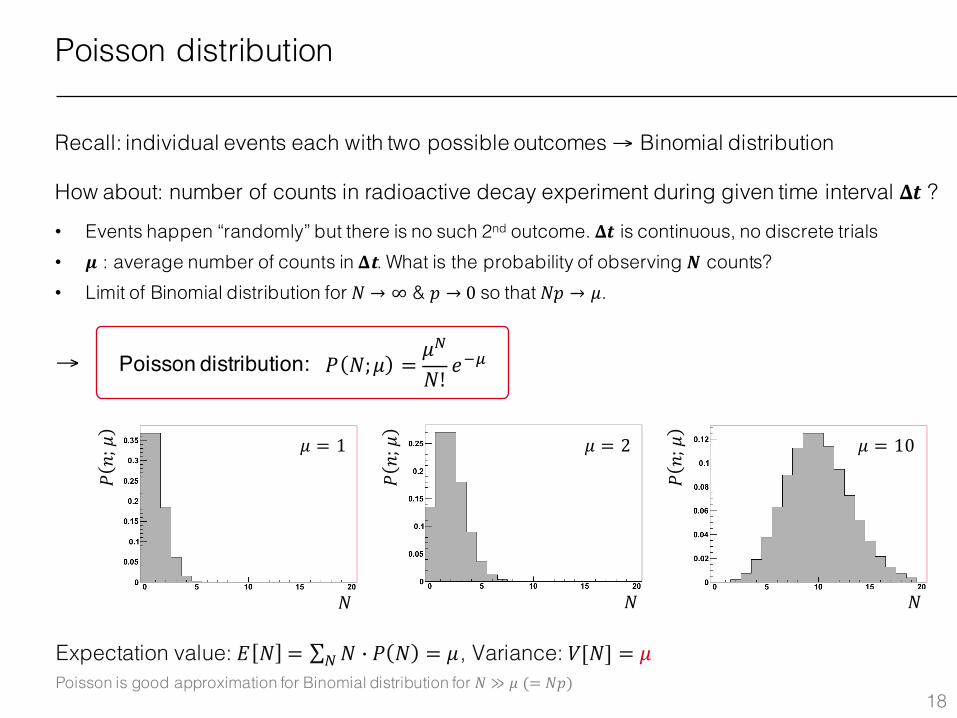
Poisson distribution

Recall: individual events each with two possible outcomes → Binomial distribution

How about: number of counts in radioactive decay experiment during given time interval 𝚫𝒕 ?

• Events happen “randomly” but there is no such 2nd outcome. 𝚫𝒕 is continuous, no discrete trials• 𝝁 : average number of counts in 𝚫𝐭. What is the probability of observing 𝑵 counts?• Limit of Binomial distribution for 𝑁 → ∞ & 𝑝 → 0so that 𝑁𝑝 → 𝜇.

18

Poisson distribution: →

Expectation value: 𝐸 𝑁 = ∑ 𝑁 j 𝑃 𝑁l = 𝜇, Variance: 𝑉[𝑁] = 𝜇Poisson is good approximation for Binomial distribution for 𝑁 ≫ 𝜇(= 𝑁𝑝)

𝑃 𝑁;𝜇 =𝜇l

𝑁!𝑒1�

𝑃𝑛;𝜇

𝑃𝑛;𝜇

𝑃𝑛;𝜇

𝑁 𝑁 𝑁

𝜇 = 1 𝜇 = 2 𝜇 = 10

Gaussian (also: “Normal”) distribution

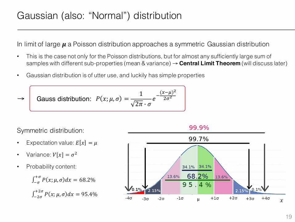
In limit of large 𝝁 a Poisson distribution approaches a symmetric Gaussian distribution

• This is the case not only for the Poisson distributions, but for almost any sufficiently large sum of samples with different sub-properties (mean & variance) → Central Limit Theorem (will discuss later)

• Gaussian distribution is of utter use, and luckily has simple properties

19

Gauss distribution: →

Symmetric distribution:

• Expectation value: 𝐸 𝑥 = 𝜇

• Variance: 𝑉[𝑥] = 𝜎x

• Probability content:

∫ 𝑃 𝑥; 𝜇, 𝜎 𝑑𝑥��1� = 68.2%

∫ 𝑃 𝑥; 𝜇, 𝜎 𝑑𝑥�x�1x� = 95.4%

𝑃 𝑥; 𝜇, 𝜎 =12𝜋 j 𝜎

𝑒1(.1�)�x��

𝑥

00.020.040.060.080.10.120.140.160.180.20.220.240.26

-4 -2 0 2 4 6 8 10 12 14

Some other distributions

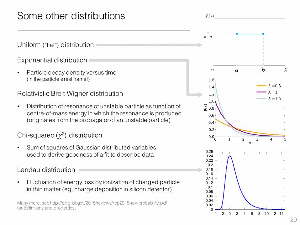
Uniform (“flat”) distribution

Exponential distribution

• Particle decay density versus time (in the particle’s rest frame!)

Relativistic Breit-Wigner distribution

• Distribution of resonance of unstable particle as function of centre-of-mass energy in which the resonance is produced (originates from the propagator of an unstable particle)

Chi-squared (𝜒2) distribution

• Sum of squares of Gaussian distributed variables; used to derive goodness of a fit to describe data

Landau distribution

• Fluctuation of energy loss by ionization of charged particle in thin matter (eg, charge deposition in silicon detector)

Many more, see http://pdg.lbl.gov/2015/reviews/rpp2015-rev-probability.pdf for definitions and properties.

07/07/2016 https://upload.wikimedia.org/wikipedia/commons/9/96/Uniform_Distribution_PDF_SVG.svg

https://upload.wikimedia.org/wikipedia/commons/9/96/Uniform_Distribution_PDF_SVG.svg 1/1

0

1b− a

a b x

f (x )

20

Central limit theorem (CLT)

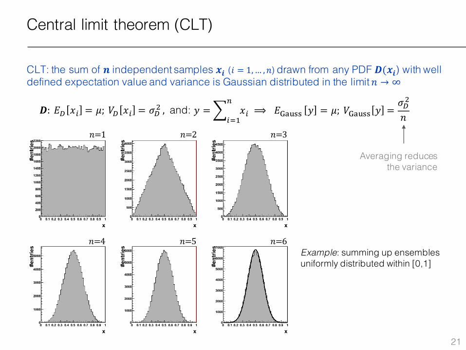
CLT: the sum of 𝒏 independent samples 𝒙𝒊 (𝑖 = 1,… , 𝑛) drawn from any PDF 𝑫(𝒙𝒊) with well defined expectation value and variance is Gaussian distributed in the limit 𝑛 → ∞

21

𝑫: 𝐸� 𝑥% = 𝜇;𝑉� 𝑥% = 𝜎�x, and:

𝑛=1

𝑛=5𝑛=4

𝑛=2 𝑛=3

𝑛=6

Averaging reduces the variance

𝑦 =3 𝑥%�

%{L⟹ 𝐸�� 77 𝑦 = 𝜇; 𝑉�� 77 𝑦 =

𝜎�x

𝑛

Example: summing up ensembles uniformly distributed within [0,1]

Central limit theorem (CLT)

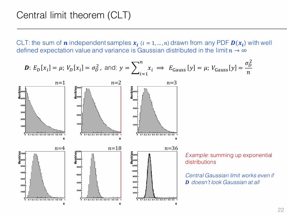
CLT: the sum of 𝒏 independent samples 𝒙𝒊 (𝑖 = 1,… , 𝑛) drawn from any PDF 𝑫(𝒙𝒊) with well defined expectation value and variance is Gaussian distributed in the limit 𝑛 → ∞

22

𝑛=1

𝑛=18𝑛=4

𝑛=2 𝑛=3

𝑛=36Example: summing up exponential distributions

Central Gaussian limit works even if 𝑫 doesn’t look Gaussian at all

𝑫: 𝐸� 𝑥% = 𝜇;𝑉� 𝑥% = 𝜎�x, and: 𝑦 =3 𝑥%�

%{L⟹ 𝐸�� 77 𝑦 = 𝜇; 𝑉�� 77 𝑦 =

𝜎�x

𝑛

10 Fundamental concepts

F(x) = L P(xd· (1.16)

A useful concept related to the cumulative distribution is the so-called quan-tile of order a or a-point. The quantile Xa is defined as the value of the random variable x such that F(xa) = 0', with 0 ::; 0' ::; 1. That is, the quantile is simply the inverse function of the cumulative distribution,

(1.17)

A commonly used special case is xl/2, called the median of x. This is often used as a measure of the typical 'location' of the random variable, in the sense that there are equal probabilities for x to be observed greater or less than xl/2.

Another commonly used measure of location is the mode, which is defined as the value of the random variable at which the p.d.f. is a maximum. A p.d.f. may, of course, have local maxima. By the most commonly used location parameter is the expectation value, which will be introduced in Section 1.5.

Consider now the case where the result of a measurement is characterized not by one but by several quantities, which may be regarded as a multidimensional random vector. If one is studying people, for example, one might measure for each person their height, weight, age, etc. Suppose a measurement is characterized by two continuous random variables x and y. Let the event A be 'x observed in [x, x + dx] and y observed anywhere', and let B be 'y observed in [y, y + dy] and x observed anywhere', as indicated in Fig. 1.4.

y 10

",I--- event A 8

4 ... .. 1' . '\ B •. -. .. ... dy

.' .. '. . 2 ... ' ..

... : . -7 E- dx

o o 2 4 6 8

x

The joint p.d.f. f(x, y) is defined by

10

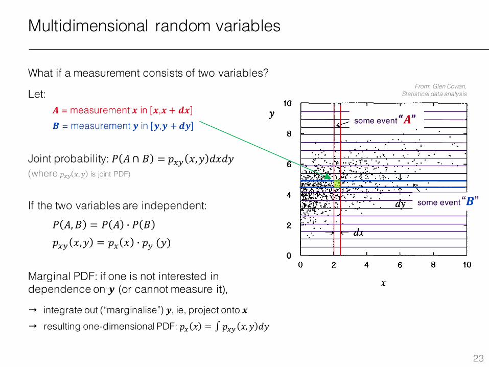
Fig. 1.4 A scatter plot of two ran-dom variables x and y based on 1000 observations. The probability for a point to be observed in the square given by the intersection of the two bands (the event A n B) is given by the joint p.d.f. times the area element, f(x, y)dxdy.

P(A n B) probability of x in [x, x + dx] and y in [y, y + dy] f(x, y)dxdy. (1.18)

i

some event “𝑨”

some event “𝑩”

Multidimensional random variables

What if a measurement consists of two variables?

Let:𝑨 = measurement 𝒙 in [𝒙,𝒙 + 𝒅𝒙]𝑩 = measurement 𝒚 in [𝒚,𝒚 +𝒅𝒚]

Joint probability: 𝑃 𝐴∩ 𝐵 = 𝑝.ª 𝑥,𝑦 𝑑𝑥𝑑𝑦(where 𝑝.ª 𝑥, 𝑦 is joint PDF)

If the two variables are independent:𝑃 𝐴, 𝐵 = 𝑃 𝐴 j 𝑃 𝐵𝑝.ª 𝑥,𝑦 = 𝑝. 𝑥 j 𝑝ª (𝑦)

Marginal PDF: if one is not interested in dependence on 𝒚 (or cannot measure it),

→ integrate out (“marginalise”) 𝒚, ie, project onto 𝒙→ resulting one-dimensional PDF: 𝑝. 𝑥 = ∫ 𝑝.ª 𝑥, 𝑦 𝑑𝑦

23

From: Glen Cowan, Statistical data analysis

Y

Xl

10

B

X2

" " " ". " 1.1.

,'II

" "

(a)

0'--_-L.J __ L----Jc...u.... __ ..1...-_----'

o 2 4 6 8 10

X

Functions of random variables 13

:5 (b) 0.4

0.3

0.2

0.1

" 0

0 2 4 6 8 10

y

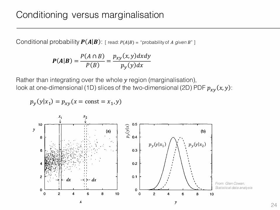
Fig. 1.6 (a) A scatter plot of random variables x and y indicating two infinitesimal bands in x of width dx at Xl (solid band) and X2 (dashed band). (b) The conditional p.d.f.s h(ylxt) and h(ylx2) corresponding to the projections of the bands onto the y axis.

I: g(xly)fy(y)dy, I: h(Ylx)fx(x)dx.

(1.27)

(1.28)

These correspond to the law of total probability given by equation (1.7), gener-alized to the case of continuous random variables.

If 'x in [x,x+dx] with any y' (event A) and 'y in [y+dy] with any x' (event B) are independent, i.e. P(A n B) = P(A) P(B), then the corresponding joint p.d.f. for x and y factorizes:

f(x, y) = fx(x) fy(y)· (1.29)

From equations (1.24) and (1.25), one sees that for independent random variables x and y the conditional p.d.f. g(xly) is the same for all y, and similarly h(ylx) does not depend on x. In other words, having knowledge of one of the variables does not change the probabilities for the other. The variables x and y shown in Fig. 1.6, for example, are not independent, as can be seen from the fact that h(ylx) depends on x.

1.4 Functions of random variables Functions of random variables are themselves random variables. Suppose a(x) is a continuous function of a continuous random variable x, where x is distributed according to the p.d.f. f(x). What is the p.d.f. g(a) that describes the distribution of a? This is determined by requiring that the probability for x to occur between

Conditioning versus marginalisation

Conditional probability 𝑷 𝑨 𝑩 : [ read: 𝑃(𝐴|𝐵) = “probability of 𝐴 given 𝐵” ]

Rather than integrating over the whole 𝑦 region (marginalisation), look at one-dimensional (1D) slices of the two-dimensional (2D) PDF 𝑝.ª 𝑥, 𝑦 :

𝑷 𝑨 𝑩 =𝑃 𝐴 ∩𝐵𝑃 𝐵

=𝑝.ª 𝑥, 𝑦 𝑑𝑥𝑑𝑦𝑝ª 𝑦 𝑑𝑥

𝑝ª 𝑦 𝑥L = 𝑝.ª(𝑥 = const = 𝑥L,𝑦)

From: Glen Cowan, Statistical data analysis

24

𝑝 ª𝑦𝑥

𝑝ª 𝑦 𝑥L 𝑝ª 𝑦 𝑥x

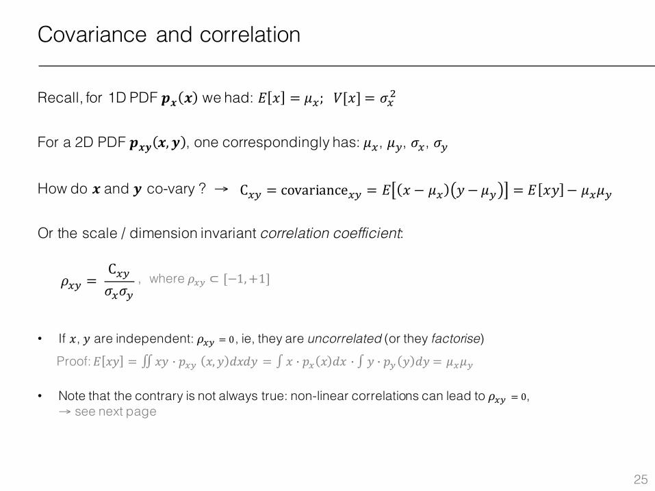
Covariance and correlation

Recall, for 1D PDF 𝒑𝒙 𝒙 we had: 𝐸 𝑥 = 𝜇.; 𝑉[𝑥] = 𝜎.x

For a 2D PDF 𝒑𝒙𝒚 𝒙, 𝒚 , one correspondingly has: 𝜇., 𝜇ª, 𝜎., 𝜎ª

How do 𝒙 and 𝒚 co-vary ? →

Or the scale / dimension invariant correlation coefficient:

C.ª = covariance.ª = 𝐸 𝑥 − 𝜇. 𝑦− 𝜇ª = 𝐸 𝑥𝑦 − 𝜇.𝜇ª

𝜌.ª = C.ª𝜎.𝜎ª

• If 𝑥, 𝑦 are independent: 𝜌.ª = 0, ie, they are uncorrelated (or they factorise)Proof:𝐸 𝑥𝑦 = ∬𝑥𝑦 j 𝑝.ª 𝑥, 𝑦 𝑑𝑥𝑑𝑦 = ∫ 𝑥 j 𝑝. 𝑥 𝑑𝑥 j ∫ 𝑦 j 𝑝ª 𝑦 𝑑𝑦 = 𝜇.𝜇ª

• Note that the contrary is not always true: non-linear correlations can lead to 𝜌.ª = 0, → see next page

, where 𝜌.ª ⊂ [−1,+1]

25

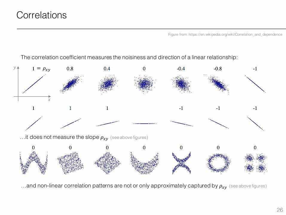
Correlations

Figure from: https://en.wikipedia.org/wiki/Correlation_and_dependence

…and non-linear correlation patterns are not or only approximately captured by 𝜌.ª (see above figures)

…it does not measure the slope 𝜌.ª (see above figures)

The correlation coefficient measures the noisiness and direction of a linear relationship:

26

𝑥

𝑦 = 𝜌.ª

Correlations

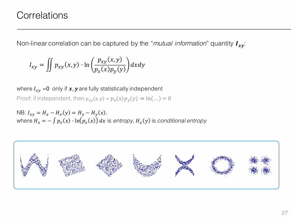
Non-linear correlation can be captured by the “mutual information” quantity 𝑰𝒙𝒚:

𝐼.ª =¶𝑝.ª 𝑥,𝑦 j ln𝑝.ª 𝑥,𝑦𝑝. 𝑥 𝑝ª 𝑦

𝑑𝑥𝑑𝑦

where 𝐼.ª =0 only if 𝒙, 𝒚are fully statistically independentProof: if independent, then 𝑝.ª 𝑥, 𝑦 = 𝑝. 𝑥 𝑝ª 𝑦 ⇒ ln … = 0

NB: 𝐼.ª = 𝐻. −𝐻. 𝑦 = 𝐻ª− 𝐻ª 𝑥 , where 𝐻. = −∫ 𝑝. 𝑥 j ln 𝑝. 𝑥 𝑑𝑥 is entropy, 𝐻. 𝑦 is conditional entropy

27

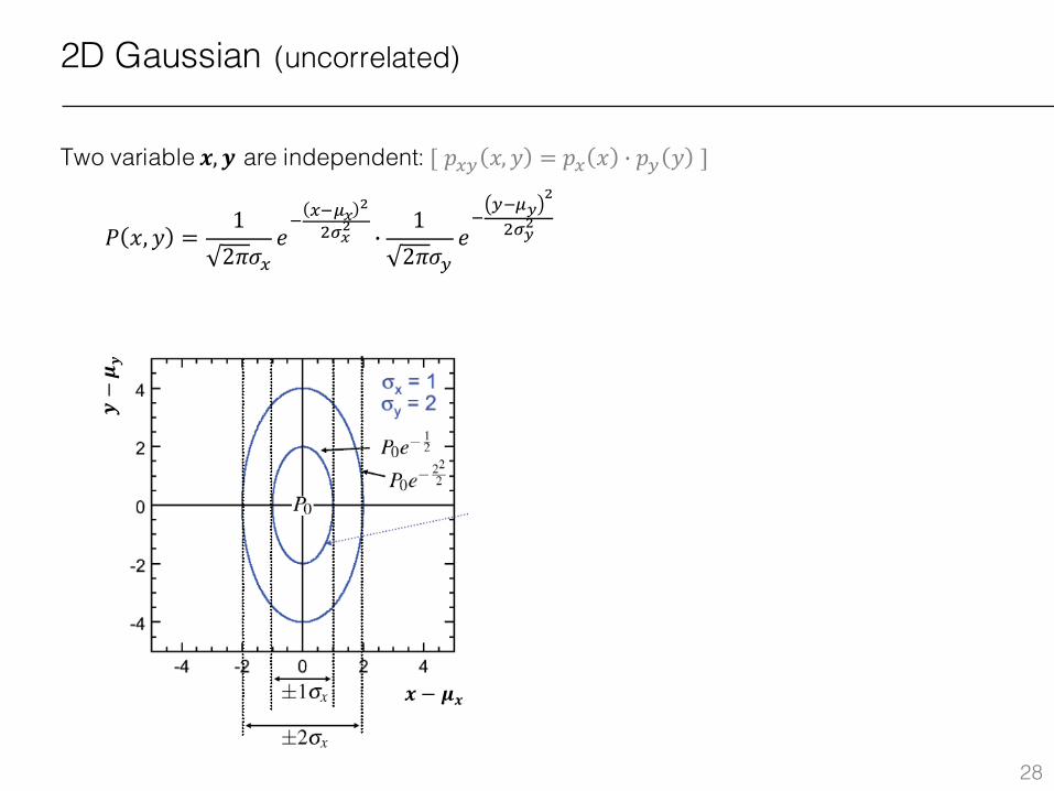
2D Gaussian (uncorrelated)

Two variable 𝒙, 𝒚 are independent: [𝑝.ª 𝑥, 𝑦 = 𝑝. 𝑥 j 𝑝ª 𝑦 ]

28

𝒙 − 𝝁𝒙

𝒚−𝝁 𝒚

𝑃 𝑥, 𝑦 =12𝜋𝜎.

𝑒1 .1�¹ �

x�¹� j12𝜋𝜎ª

𝑒1ª1�º

�

x�º�

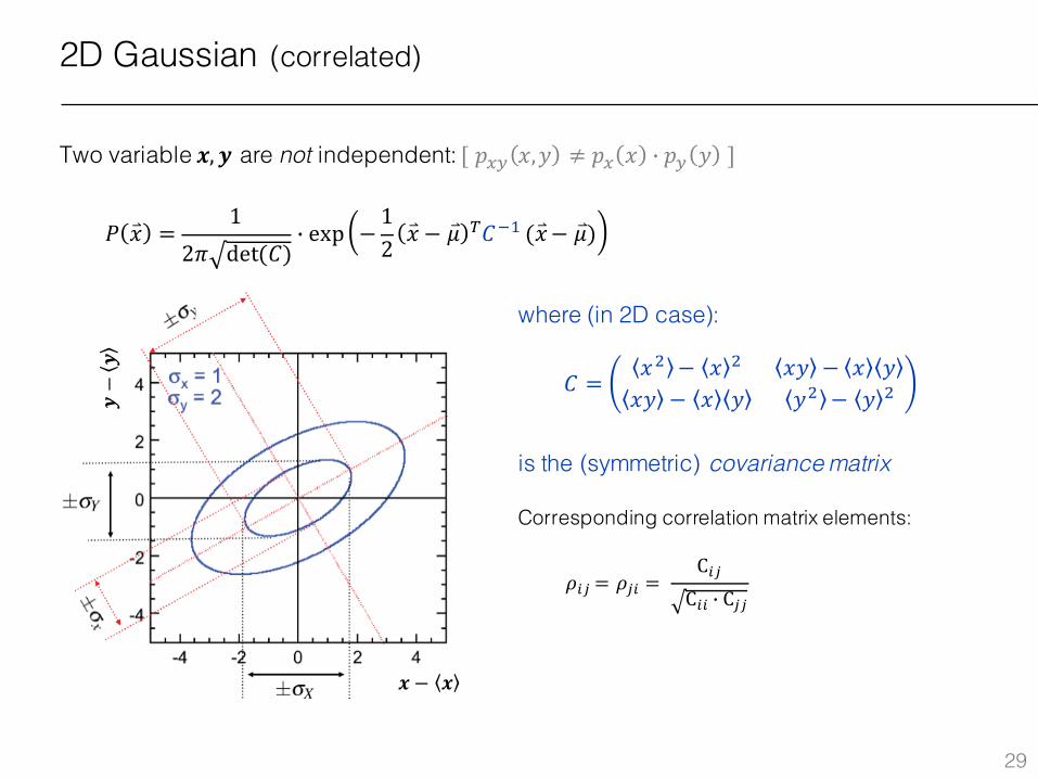
2D Gaussian (correlated)

Two variable 𝒙, 𝒚 are not independent: [𝑝.ª 𝑥,𝑦 ≠ 𝑝. 𝑥 j 𝑝ª 𝑦 ]

29

where (in 2D case):

is the (symmetric) covariance matrix

Corresponding correlation matrix elements:

𝑃 �⃑� =1

2𝜋 det(𝐶)j exp −

12�⃑� − 𝜇 À𝐶1L(�⃑�− 𝜇)

𝜌%Á = 𝜌Á% = C%ÁC%% j CÁÁ

𝐶 =𝑥x − 𝑥 x 𝑥𝑦 − 𝑥 𝑦𝑥𝑦 − 𝑥 𝑦 𝑦x − 𝑦 x

𝒙 − 𝒙

𝒚−𝒚

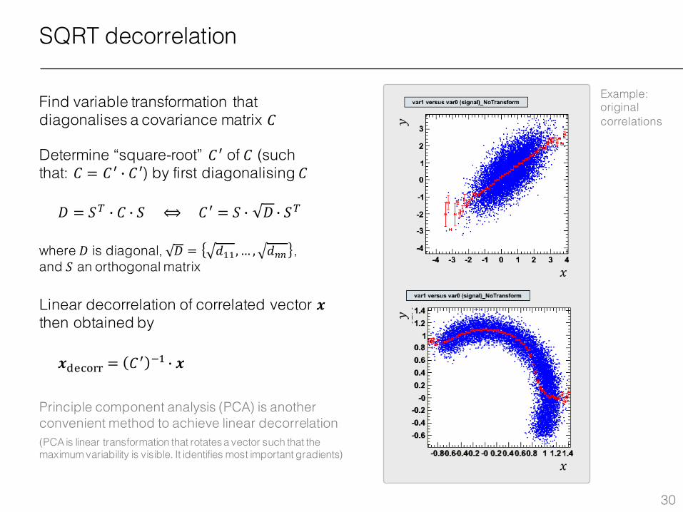
SQRT decorrelation

Find variable transformation that diagonalises a covariance matrix 𝐶

Determine “square-root” 𝐶Â of 𝐶 (such that: 𝐶 = 𝐶Â j 𝐶Â) by first diagonalising 𝐶

𝐷 = 𝑆À j 𝐶 j 𝑆 ⟺𝐶Â = 𝑆 j 𝐷 j 𝑆À

where 𝐷 is diagonal, 𝐷 = 𝑑LL,… , 𝑑�� , and 𝑆 an orthogonal matrix

Linear decorrelation of correlated vector 𝒙then obtained by

𝒙;8Æ599 = 𝐶Â 1L j 𝒙

Principle component analysis (PCA) is another convenient method to achieve linear decorrelation (PCA is linear transformation that rotates a vector such that the maximum variability is visible. It identifies most important gradients)

Example: original correlations

30

𝑥

𝑥

𝑦𝑦

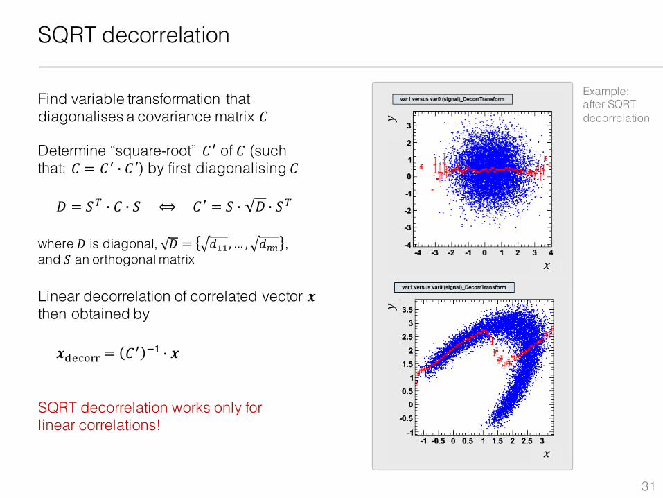
SQRT decorrelation

Example: after SQRT decorrelation

SQRT decorrelation works only for linear correlations!

Find variable transformation that diagonalises a covariance matrix 𝐶

Determine “square-root” 𝐶Â of 𝐶 (such that: 𝐶 = 𝐶Â j 𝐶Â) by first diagonalising 𝐶

𝐷 = 𝑆À j 𝐶 j 𝑆 ⟺𝐶Â = 𝑆 j 𝐷 j 𝑆À

where 𝐷 is diagonal, 𝐷 = 𝑑LL,… , 𝑑�� , and 𝑆 an orthogonal matrix

Linear decorrelation of correlated vector 𝒙then obtained by

𝒙;8Æ599 = 𝐶Â 1L j 𝒙

31

𝑥

𝑥

𝑦𝑦

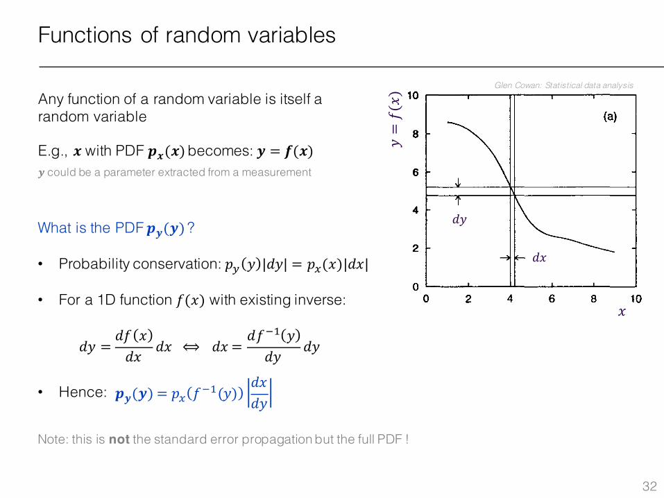
Functions of random variables

Any function of a random variable is itself a random variable

E.g., 𝒙 with PDF 𝒑𝒙(𝒙)becomes: 𝒚 = 𝒇(𝒙)𝒚 could be a parameter extracted from a measurement

32

What is the PDF 𝒑𝒚(𝒚)?

• Probability conservation: 𝑝ª 𝑦 |𝑑𝑦| = 𝑝.(𝑥)|𝑑𝑥|

• For a 1D function 𝑓(𝑥) with existing inverse:

• Hence:

𝑑𝑦 =𝑑𝑓 𝑥𝑑𝑥

𝑑𝑥⟺ 𝑑𝑥 =𝑑𝑓1L 𝑦𝑑𝑦

𝑑𝑦

𝒑𝒚(𝒚) = 𝑝. 𝑓1L(𝑦)𝑑𝑥𝑑𝑦

Note: this is not the standard error propagation but the full PDF !

14 Fundamental concepts

.--.. 10 3: 10

(b) 8 8

6 6

4 4

2 2

0 0 0 2 4 6 8 10 0 2 4 6 8 10

x x

Fig. 1.7 Transformation of variables for (a) a function q( x) with a single-valued inverse x( a) and (b) a function for which the interval da corresponds to two intervals dXl and dX2'

x and x + dx be equal to the probability for a to be between a and a + da. That IS,

g(a')da' = 1 J(x)dx, dS

(1.30)

where the integral is carried out over the infinitesimal element dS defined by the region in x-space between a (x) = a' and a (x) = a' + da', as shown in Fig. 1. 7 ( a) . If the function a(x) can be inverted to obtain x(a), equation (1.30) gives

11x (a+da) I l x (aH, *,da

g(a)da = J(x')dx' = J(x')dx', x(a) x(a)

(1.31)

or

g(a) = f(x(a)) 1 I· (1.32)

The absolute value of dx/da ensures that the integral is positive. If the function a(x) does not have a unique inverse, one must include in dS contributions from all regions in x-space between a(x) = a' and a(x) = a' +da', as shown in Fig. 1.7(b).

The p.d.f. g(a) of a function a(xl, ... , xn) of n random variables Xl, ... , Xn with the joint p.d.f. J(XI,.'" xn) is determined by

g(a')da' = J .. ·15 J(XI, ... , Xn)dXI ... dxn, (1.33)

where the infinitesimal volume element dS is the region in Xl, ... ,xn-space be-tween the two (hyper)surfaces defined by a(xI, ... , xn) = a' and a(xI, ... , xn) = a' + da'.

𝑑𝑦

𝑦=𝑓(𝑥)

Glen Cowan: Statistical data analysis

𝑑𝑥

𝑥

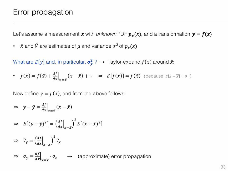
Error propagation

Let’s assume a measurement 𝒙 with unknown PDF 𝒑𝒙(𝒙), and a transformation 𝒚 = 𝒇(𝒙)

• �̅� and 𝑉Ê are estimates of 𝜇 and variance 𝜎xof 𝑝.(𝑥)

What are 𝐸 𝑦 and, in particular, 𝝈𝒚𝟐 ? → Taylor-expand 𝑓 𝑥 around �̅�:

• 𝑓 𝑥 = 𝑓 �̅� + ÍÎÍ.Ï.{.̅

𝑥 − �̅� +⋯ ⇒ 𝐸 𝑓 𝑥 ≃ 𝑓 �̅� (because: 𝐸 𝑥 − 𝑥Ñ = 0 !)

Now define 𝑦Ò = 𝑓 �̅� , and from the above follows:

⬄ 𝑦− 𝑦Ò ≃ ÍÎÍ.Ï.{.̅

𝑥 − �̅�

⬄ 𝐸 (𝑦− 𝑦Ò)x = ÍÎÍ.Ï.{.̅

x𝐸 (𝑥 − �̅�)x

⬄ 𝑉ʪ =ÍÎÍ.Ï.{.̅

x𝑉Ê.

⬄ 𝜎ª =ÍÎÍ.Ï.{.̅

j 𝜎.

33

→ (approximate) error propagation

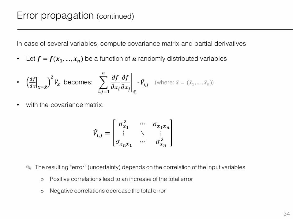
Error propagation (continued)

In case of several variables, compute covariance matrix and partial derivatives

• Let 𝒇 = 𝒇(𝒙𝟏, … , 𝒙𝒏) be a function of 𝒏 randomly distributed variables

• ÍÎÍ.Ï.{.̅

x𝑉Ê. becomes: (where: �̅� = (�̅�L,… , �̅��))

• with the covariance matrix:

34

3𝜕𝑓𝜕𝑥%

𝜕𝑓𝜕𝑥Á

Õ.̅

�

%,Á{L

j 𝑉Ê%,Á

𝑉Ê%,Á =𝜎.Öx ⋯ 𝜎.Ö.×⋮ ⋱ ⋮

𝜎.×.Ö ⋯ 𝜎.×x

® The resulting “error” (uncertainty) depends on the correlation of the input variables

o Positive correlations lead to an increase of the total error

o Negative correlations decrease the total error

35

Probability and statistics are everywhere in science, and in particular profoundly contained in particle physics and in the physics of large ensembles

Overview of some important probability density distributions given, also:

• Joint / marginal / conditional probabilities

• Covariance and correlations

• Error propagation

Next: how to use these concepts for hypothesis testing

Summary for today