Introduction to loop quantum gravity

Suvi-Leena Lehtinen

21.9.2012

Submitted in partial fulfilment of the requirements

for the degree of Master of Science of Imperial College London

1

Abstract

Loop quantum gravity is an attempt to formulate a quantum theory of general rel-

ativity. The quantisation is performed in a mathematically rigorous, non-perturbative

and background independent manner and standard matter couplings are considered.

This dissertation considers the foundations required to build the theory, general rela-

tivity as a Hamiltonian system and quantisation of gravity in the spin network basis.

Some applications and results of loop quantum gravity are presented: loop quantum

cosmology and the removal of singularities, black hole entropy, and the modern spin-

foam formalism. The current status of loop quantum gravity research is discussed.

2

Contents

1 Introduction 4

2 General relativity 7

2.1 Tetrad formalism . . . . . . . . . . . . . . . . . . . . . . . . . . . . . . . . . 7

2.2 Gauge invariance . . . . . . . . . . . . . . . . . . . . . . . . . . . . . . . . . 8

2.3 3 + 1 decomposition - splitting of spacetime . . . . . . . . . . . . . . . . . . 10

3 Constraint mechanics 11

3.1 Non-relativistic mechanics . . . . . . . . . . . . . . . . . . . . . . . . . . . . 11

3.2 Relativistic mechanics . . . . . . . . . . . . . . . . . . . . . . . . . . . . . . 13

4 Ashtekar variables 13

5 Quantum theory 17

5.1 Holonomies . . . . . . . . . . . . . . . . . . . . . . . . . . . . . . . . . . . . 17

5.2 Wilson loops . . . . . . . . . . . . . . . . . . . . . . . . . . . . . . . . . . . 18

5.3 Spin network states . . . . . . . . . . . . . . . . . . . . . . . . . . . . . . . . 20

5.4 Loop representation of operators . . . . . . . . . . . . . . . . . . . . . . . . 21

5.5 Quantisation of the Hamiltonian constraint . . . . . . . . . . . . . . . . . . 26

5.6 Coupling to matter . . . . . . . . . . . . . . . . . . . . . . . . . . . . . . . . 28

6 An application: loop cosmology 29

6.1 Isotropic spacetime . . . . . . . . . . . . . . . . . . . . . . . . . . . . . . . . 30

6.2 Discrete scale factor . . . . . . . . . . . . . . . . . . . . . . . . . . . . . . . 32

6.3 Dynamics . . . . . . . . . . . . . . . . . . . . . . . . . . . . . . . . . . . . . 34

6.4 Removal of singularity . . . . . . . . . . . . . . . . . . . . . . . . . . . . . . 35

6.5 Inflation . . . . . . . . . . . . . . . . . . . . . . . . . . . . . . . . . . . . . . 35

7 Black hole entropy 36

8 Spinfoam formalism 40

9 Some open problems 43

10 Conclusion 45

3

1 Introduction

The quantum nature of three of the four forces, electromagnetism, weak and strong interac-

tions, suggest that gravitational force too should have quantum properties at Planck scales.

Loop quantum gravity (LQG) is an attempt to quantise gravity in a non-perturbative and

background independent way. This section introduces the reader to the ideas behind loop

quantum gravity.

Why must one quantise? Quantum mechanics has an external time variable, t in the

Schrodinger equation, or alternatively in quantum field theory a fixed non-dynamical back-

ground. On the other hand, in general relativity the metric is a smooth deterministic

dynamical field. But in quantum mechanics any dynamical field is quantised, hence the

gravitational field should be quantised.

General relativity has two main properties: diffeomorphism invariance and background

independence. General relativity could be viewed as a field theory from the form of the

Einstein-Hilbert action but this form does not influence the notions of space and time.

Only diffeomorphism invariance and background independence are important. The task is

to find a background independent quantum field theory or a general relativistic quantum

field theory.

There are several attempts at quantising gravity, the most developed of which are loop

quantum gravity and string theory. Other approaches are dynamical triangulations, non-

commutative geometry, Hartle’s quantum mechanics of spacetime, Hawking’s Euclidean

sum over geometries, quantum Regge calculus, Penrose’s twistor theory, Sorkin’s causal

set, t’Hooft’s deterministic approach and Finkelstein’s theory.

The main competing theory of loop quantum gravity, namely string theory, assumes that

elementary objects are extended rather than point-like. String theory is successful in the

sense that it contains a lot of phenomenology but on the cost of having to introduce

supersymmetry, extra dimensions and an infinite number of fields with arbitrary masses

and spins. The aim of string theory is broader than that of loop quantum theory, since it

unifies gravity with the other forces. Loop quantum gravity does not attempt to unify, only

find a background independent quantum field theory. While string theory is perturbative,

loop quantum gravity is non-perturbative. It leads to a discrete structure of spacetime at

the Planck scale. Loop quantum gravity is UV divergence free; the UV divergences of QFT

4

are a consequence of the assumption that the background geometry is smooth.

How does one think in loop quantum gravity? Loop quantum gravity is based on the

assumption that quantum mechanics and general relativity are correct. It assumes back-

ground independence and does not attempt to unify forces, only to quantise gravity. Space-

time is assumed to be four-dimensional and no supersymmetry is required but the possi-

bility of supersymmetry is not excluded.

One must step away from the idea that the world inhabits space and evolves in time. This

is because spacetime itself is dynamical so spacetime is constructed from the quanta of the

gravitational field. The absence of spacetime is what is called background independence.

Background independence is manifested as diffeomorphism invariance of the action. Dif-

feomorphism invariance means that the action is invariant under coordinate change and

that it lacks a non-dynamical background field.

Loop quantum gravity although looking for a general relativistic quantum field theory

does not use conventional quantum field theory because quantum field theory is defined

in a background dependent way. Instead loop quantum gravity uses the Hilbert space

of states, operators and transition amplitudes of traditional quantum mechanics. The

canonical algebra of fields with positive and negative frequency components is replaced by

an algebra of matrices of parallel transport along closed curves. These matrices are called

holonomies or Wilson loops.

The holonomies are the essence of loop quantum gravity as they, on quantisation, become

operators that create loop states. A loop state transforms under an infinitesimal transfor-

mation into an equivalent representation of the same state. Finite transformations change

the state into a different one. This is because only the relative position of the loop with

respect to other loops is significant.

The states in loop quantum gravity are solutions of the generalised Schrodinger equation

called the Wheeler-DeWitt equation

HΨ = 0, (1)

where H is the relativistic Hamiltonian or Hamiltonian constraint and Ψ is the space of

solutions to the equation. The right-hand side is zero since space and time are on an equal

footing in loop quantum gravity, so there is no external time variable to differentiate by.

5

Construction of the Hamiltonian is a significant issue in the theroy and there is more than

one version of the constraint.

The space of solutions can be expressed in terms of an orthogonal basis of spin network

states. Spin network states are finite linear combinations of loop states. H acts only on

the nodes of a spin network, hence a loop or a set of non-intersecting loops solves the

Wheeler-DeWitt equation.

In this spin network basis, a set of quantum operators can be defined. The area and volume

operators have discrete spectra. The eigenvalues of the area operator are

A = 8πγ~G∑i

√ji(ji + 1) (2)

where ji are labels on the spin network and γ is the Immirzi parameter. Hence the size of

a quantum of space is determined to some extent by the Immirzi parameter.

Loop quantum gravity has been applied to cosmology with some interesting results. The

discreteness of physical space implies that the Big Bang singularity of classical cosmology

is removed and replaced instead by the Big Bounce where evolution can be continued past

the classical singularity. A universe that contracts bounces back to an expanding phase and

vice versa under this result. Loop quantum cosmology is successful in describing flat and

homogeneous models but investigating more complicated models requires more developed

numerical methods.

As well as cosmology, loop quantum gravity can be applied to the study of black holes.

Loop quantum gravity is consistent with the Bekenstein-Hawking entropy formula and it

predicts a logarithmic quantum correction to the entropy formula.

An extension of traditional loop quantum gravity is the path integral formalism, which is

based on spinfoams. Spinfoams are like the world-surface of a spin network evolving in

time. The spinfoam formalism is a very active area of research and a major result is that

the graviton propagator, or Newton’s law in the classical limit, has been found.

While loop quantum gravity has produced lots of results, there are gaps to fill in. One

of them is the low-energy limit: does loop quantum gravity have general relativity as the

correct low-energy limit. At present loop quantum gravity, like all theories of quantum

gravity, lacks experimental verification. It may be possible to get predictions from loop

6

cosmology that could be verified by experiment, though this is still far from being the

case.

There are a few books that present the theory of loop quantum gravity and its history. A

comprehensive one is Rovelli (2004) [1], and from a slightly different point of view Gambini

and Pullin (1997) [2]. They do not include many technical details, however Thiemann

(2007) [3] presents thorough derivations. A new book that is accessible to undergraduates is

Gambini and Pullin (2011) [4]. A reader of popular science books may find Smolin’s Three

roads to quantum gravity [5] interesting. For applications to loop quantum cosmology

there are good review articles, for example [6] and [7]. Spinfoam formalism is introduced

for example in [8] The next sections delve into the details of what has been said in this

section.

2 General relativity

This section gives an introduction to the background material needed for the theory of

loop quantum gravity following [1].

2.1 Tetrad formalism

The tetrad formalism is a standard formalism of GR and it was used as a basis for the

later formalisms. This section contains standard material which is covered thoroughly in

Wald’s book [9] and briefly in [1].

In the tetrad formalism the gravitational field, or tetrad field, is a one-form eI(x) =

eIµ(x)dxµ where µ is a spacetime tangent index and I are components of a Minkowski vector

raised and lowered with the Minkowski metric. The spin connection ωIJ(x) = ωIµJ(x)dxµ,

with I, J being Lorentz indices, is a one-form with values in the Lie algebra of the Lorentz

group. The covariant partial derivative is defined by acting with it on a vector field

DµvI = ∂µv

I + ωIµJvJ .

A gauge covariant derivative on a one-form is DuI = duI + ωIJ ∧ uJ and the torsion is

T I = DeI = deI+ωIJ∧eJ . The torsion is zero for a torsion-free spin connection. Curvature

7

is given by RIJ = dωIJ +ωIK ∧ωKJ . The torsion and curvature expressions are the famous

Cartan structure equations.

The action that gives rise to the Einstein equations and determines that torsion is zero is

the action

S[e, ω] =1

16πG

∫εIJKL(

1

4eI ∧ eJ ∧R[ω]KL − 1

12λeI ∧ eJ ∧ eK ∧ eL), (3)

where λ is the cosmological constant and G is Newton’s constant.

As well as the gravitational field there is matter - Yang-Mills fields, fermion fields and

scalar fields. These can be described with the following actions. For a connection A and

curvature F the Yang-Mills action is

SYM [e,A] =1

4

∫Tr[F ? ∧ F ], (4)

with the trace being the trace on the algebra. Scalars and fermions can be added simi-

larly.

Varying the total action including the matter terms with respect to e leads to the Einstein

equations

εIJKL(eI ∧RJK − 2

3λeI ∧ eJ ∧ eK) = 2πGTL (5)

with the usual definition of the energy-momentum three-form

TI(x) =δSmatterδeI(x)

. (6)

2.2 Gauge invariance

Gauge invariance plays a crucial role in loop quantum gravity so the gauge transformations

of the Standard Model are listed here. The equations of motion derived from the G =

SU(3)× SU(2)×U(1) model action are invariant under local Yang-Mills transformations,

Lorentz transformations and diffeomorphisms. These three maps transform a solution

of the equations of motion into another solution. These transformations leave physical

quantities invariant. If a local quantity depends on a fixed point it is not diffeomorphism

invariant. The maps are the following: Local Yang-Mills transformations are given by the

8

map λ :M→ G

λ : φ(x) 7→ Rφ(λ(x))φ(x)

ψ(x) 7→ Rψ(λ(x))ψ(x)

Aµ(x) 7→ R(λ(x))Aµ(x) + λ(x)∂µλ−1(x)

eIµ(x) 7→ eIµ(x)

ωIµJ(x) 7→ ωIµJ(x),

(7)

where R is in the adjoint representation of the group G and Rφ and Rψ are in the repre-

sentations of G that contain φ and ψ respectively.

Local Lorentz transformations are give by the map λ :M→ SO(3, 1)

λ : φ(x) 7→ φ(x)

ψ(x) 7→ S(λ(x))ψ(x)

Aµ(x) 7→ Aµ(x)

eIµ(x) 7→ λIJ(x)eJµ(x)

ωIµJ 7→ λIK(x)ωKµL(x)λLJ (x) + λIK(x)∂muλKJ (x),

(8)

where λIJ ∈ SO(3, 1).

A diffeomorphism is a smooth invertible map φ :M→M

φ : ϕ(x) 7→ ϕ(φ(x))

ψ(x) 7→ ψ(φ(x))

Aµ(x) 7→ ∂φν

∂xµAν(φ(x))

eIµ(x) 7→ ∂φν

∂xµeIν(φ(x))

ωIµJ 7→∂φν

∂xµωIνJ(φ(x)),

(9)

Any physical quantity must be invariant under these transformations.

9

2.3 3 + 1 decomposition - splitting of spacetime

The Hamiltonian formalism of general relativity is a step towards quantising general rela-

tivity. In order to combine general relativity with standard quantum mechanics, spacetime

must be split into spatial slices and time. This is required as the Hamiltonian formalism

gives the evolution of fields with respect to a time variable. Although picking a time di-

rection breaks covariance, the choice of the time direction was entirely arbitrary and hence

covariance is restored later. The Hamiltonian formulation of general relativity was created

by Arnowitt, Deser and Misner, whose work appeared in [10]. Details about this section

are in [2] and [3].

Figure 1: Split of spacetime into spatial slices of constant t and the lapse N and shift Na

indicated in the figure from [3]

To make the split into space and time assume that the four-dimensional spacetime manifold

M with a metric gab can be split as M ∼= Σ × R, where Σ is a three-dimensional spatial

slice. Let t label the constant spatial slices Σ and nµ be a normal to Σ. Then define the

spatial three-metric qab as

qab ≡ gab + nanb. (10)

It is easiest to think that in this expression a, b = 1, 2, 3. Then one can decompose a vector

ta into components normal and tangential to Σ as

ta = Nna +Na. (11)

10

N is called the lapse and is related to moving between spatial slices, while Na is called the

shift vector which transports along the spatial slice Σ (see figure 1). Here t has indices 0

to 3 but only N not Na contributes to the zeroth component.

On the four-dimensional manifold one can now choose coordinates (t, xa), with a = 1, 2, 3

coordinates on the spatial slice, with which the metric becomes

ds2 = (−N2 +NaNa)dt2 + 2Nadtdx

a + qabdxadxb. (12)

It will be useful later to consider the extrinsic curvature of the spatial slices. The extrinsic

curvature measures the change in the three-dimensional metric moving from one slice to

another. The extrinsic curvature is defined as

Kab ≡ qcaqdb∇cnd =1

2Lnqab. (13)

Also,

qab ≡ L~tqab = 2NKab + L ~Nqab. (14)

The extrinsic curvature is related to the conjugate momentum of the metric, which along-

side with the metric will be a canonical variable.

3 Constraint mechanics

Ordinary non-relativistic Hamiltonian mechanics relies on having a time variable to describe

evolution. In general relativity however, there is not an external time variable so ordinary

mechanics is not broad enough to describe general relativistic systems. The aim is to

find a formulation which is as close to quantum mechanics as possible. Let’s start with

non-relativistic mechanics. This section follows [1].

3.1 Non-relativistic mechanics

The dynamics of a non-relativistic system is specified by a lagrangian L(qi, vi) = L(qi(t), dqi(t)dt )

where i runs over the number of degrees of freedom m of the system and qi are values in the

11

configuration space. The allowed motion is then given by an extremum of the action

S[q] =

t2∫t1

L(qi(t),dqi(t)

dt)dt. (15)

The extrema are given by the Euler-Lagrange equations or equivalently Hamilton’s equa-

tions. The Hamilton-Jacobi equation, which can be derived by taking the classical limit of

the Schrodinger equation, is

∂S(qi, t)

∂t+H0(qi,

∂S(qi, t)

∂qi) = 0, (16)

where H0 is the non-relativistic Hamiltonian and S(qi, t) is the action evaluated along the

classical trajectory with end-point (qi, t).

Solutions of the Hamilton-Jacobi equation can be found in the form S(qi, Qi, t) = Et −W (qi, Qi), where E is a constant and W, the characteristic Hamilton-Jacobi function,

satisfies

Ho(qi,∂W (qi, Qi)

∂qi) = E. (17)

S(qi, Qi, t) is called the principal Hamilton-Jacobi function. Once those have been found,

the solutions of the equation of motion qi can be found by first calculating

P i(qi, Qi, t) = −∂S(qi, Qi, t)

∂Qi, (18)

and then inverting the equation to qi(t) = qi(Qi, Pi, t). Pi are integration constants.

Another form of solution of the Hamilton-Jacobi equation is the Hamilton function S(t1, qi1, t2, q

i2),

a function in the configuration space between (t1, qi1) and (t2, q

i2) given by

S(t1, qi1, t2, q

i2) =

t2∫t1

dtL(qi(t), qi(t)), (19)

where qi again minimises the action. The Hamilton function has the quantum propagator

as its classical limit.

12

3.2 Relativistic mechanics

The Hamilton-Jacobi formulation can be extended to include relativistic systems.

All relativistic systems excluding quantum effects can be described by the following set:

1. Relativistic configuration space C of partial observables

2. Relativistic phase space Γ of relativistic states

3. Evolution equation f = 0 for the map to a linear space V f : Γ× C → V

The relativistic Hamilton-Jacobi equation is given by

H(qa,∂S(qa)

∂qa) = 0 (20)

where qa are the observables. Notice that this is simpler than (16) since an external time

variable cannot be specified. The evolution equation is

f i(qa, Pi, Qi) ≡ ∂S(qa, Qi)

∂Qi+ Pi = 0. (21)

4 Ashtekar variables

General relativity can be expressed in terms of a three dimensional SU(2) connection Aia

and a real three dimensional momentum conjugate, the densitised triad Eai =√

detqEaiwith

Eai =∂S[A]

∂Aia. (22)

Both sets of indices run from 1 to 3. Indices a denote vector indices in curved space and i

are internal indices raised and lowered with the flat metric δij . This new formulation of GR

was introduced by Abhay Ashtekar in his paper [11] in 1986. The tildes will be dropped

for convenience; Eai now refers to the densitised triad. The variables in his formulation

have the Poisson bracket

AiA(x), Ebj (y) = 8πGγδab δijδ

3(x− y) (23)

13

where γ is a complex constant called Barbero-Immirzi parameter. Theories with different

γ’s are related by canonical transformation variables. The importance of the Immirzi

parameter for quantum theory was pointed out in [12].

In Ashtekar formulation the spatial metric can be written in terms of the triad as

qab = Eai Ebjδij . (24)

The connection Aia is related to the spin connection Γia = Γajkεjki and the extrinsic curva-

ture by

Aia = Γia + γKia (25)

with K the extrinsic curvature Kia = KabE

ai/√

det(q). The definition of Kab was given in

(13).

In terms of these variables the Einstein-Hilbert action,

S =1

16πG

∫d4x√−det(g)R, (26)

with R the Ricci scalar, becomes (see e.g. [1])

L =1

8πGγ

∫d3x(Eai A

ia +NεijkE

ai E

bjF

kab +NaEbiF

iab + λi(DaE

a)i) (27)

where γ has been set to i and Da is the covariant derivative with Aik and F iab is the

curvature. Explicitly,

Davi = ∂avi + εijkAjavk

F iab = ∂aAib − ∂bAia + εijkA

jaA

kb

(28)

In the Lagrangian (27), the 00 and 0i components of the metric g have been replaced by

the shift and lapse functions (see equation 11), as g00 = 1/N2 and g0i = N i/N2. The lapse

N and shift Na and the gauge parameter λi are Lagrange multipliers. This means that

there are seven constraints given by [13], [14]

Gi = DaEai = 0,

Vb = Eai Fiab = 0,

H = εijkEai E

bjF

kab = 0,

(29)

14

G is called the Gauss’ law, V is the momentum or vector constraint and H is the Hamilto-

nian constraint. The Hamiltonian constraint generates the time evolution in terms of the

zeroth component of the x-coordinate. The total Hamiltonian of GR is a linear combination

of these constraints as can be seen from the Lagrangian.

It is useful to smear the constraints so that the Gauss law becomes

G[λ] = −∫

d3xλiDaEai =

∫d3xDaλ

iEai = 0, (30)

The diffeomorphism constraint, the generator of pure diffeomorphisms, is a combination

of Gauss’ law and momentum constraint Ca = Va − Aia(DbEbi ) with the smeared form

being

C( ~N) =

∫d3xNaCa. (31)

The Poisson bracket of the diffeomorphism constraint with a function of the canonical

variables is just the Lie derivative along ~N [4]

C( ~N), f(E,A) ∼ L ~Nf (32)

For the Hamiltonian constraint, which is a density of weight two, it is convenient to divide it

by a density of weight one to enable the integration to be defined. Using the volume

V =

∫d3x√|det(E(x))| (33)

and its commutator with the Ashtekar connection (γ = i)

V, Aia(x) = (8πiG)Ebj (x)Eck(x)εabcε

ijk

4√|detE(x)|

(34)

the Hamiltonian constraint can be written in the following useful form [15]:

H[N ] =

∫N Tr(F ∧ V, A) = 0. (35)

On a further note, GR is a totally constrained system with the Hamiltonian written ex-

15

plicitly in Ashtekar variables i.e.

H =

∫d3xNεijkEai EbjF kab +NaEbiF

iab + λi(DaE

a)i. (36)

This is for Barbero-Immirzi parameter γ = i. If one restricts γ to a real number then

one obtains Lorentzian GR where everything else stays the same except the Hamiltonian

constraint is then [16]

H = εijkEai E

bjF

kab + 2

γ2 + 1

γ2(Eai E

bj − EajEbi )(Aia − Γia)(A

jb − γ

jb ) = 0. (37)

Details about the new second term in the Hamiltonian and its implications are in [3].

It is important to consider the constraint algebra because the constraints of the theory must

be constant over time. This means that their Poisson bracket with the total Hamiltonian

must be zero. The total Hamiltonian is a linear combination of constraints, hence the

Poisson brackets among constraints must be proportional to constraints [4]. Consider the

smeared versions of the constraints, the smeared Hamiltonian constraint being

H(N) =

∫d3xN

EaiEbjF kabεijk√det(q)

, (38)

the Gauss constraint (30) and diffeomorphism constraint (31). The constraint algebra is

then [4]

G(λ), G(µ) = G([λ, µ]), (39)

with [λ, µ]i = λjµkεijk, i.e. the commutator of two smearing constants or Lagrange multi-

pliers. Most of the other Poisson bracket brackets are simple, the diffeomorphism simply

shifts the smearing so

C( ~N), C( ~M) = C(L ~NM), (40)

C( ~N), G(λ) = G(L ~Nλ), (41)

G(λ), H(M) = 0, (42)

C( ~N), H(M) = H(L ~NM), (43)

H(N), H(M) = C( ~K). (44)

16

with

Ka = Eai Ebi(N∂bM −M∂bN)/det(q). (45)

The last Poisson bracket, the bracket of two Hamiltonian constraints is different because

it depends on the canonical variables, which will become quantum operators.

5 Quantum theory

Loop quantum gravity builds on holonomies, which are introduced below. These are crucial

for quantising the gravitational theory. The states of the theory, spin networks, are formed

from closed loops. Quantum operators act on these and the quantum structure of spacetime

turns out to be discrete. Further, the constraints are quantised and matter can also be

included.

5.1 Holonomies

This section discusses the concept of holonomies following [2]. Holonomies are important

because all observables that are functions of the connection only, can be expressed in a

basis of holonomies. A holonomy H(γ) is the parallel transport along a closed curve γ

with a basepoint. The holonomy has the same information in it as the curvature: know-

ing all holonomies of the one-form connection Aia defines the connection uniquely [17].

The holonomy for any closed curve implies the connection at any point modulo a gauge

transformation.

Two closed curves are equivalent if one can be continuously deformed to the other. All

loops which are equivalent form an equivalence class. The equivalence classes of closed

curves form a group structure, and holonomies can be thought of as a map from this group

onto a Lie group G. Technically the equivalence classes of closed curves are called loops

and the group a group of loops. Functions of the elements in the group of loops are called

wavefunctions and these form the loop representation. Explanation of all of this in more

detail follows.

The group of loops is really a semi-group. Consider the set of closed curves with a start

and end point at o. The identity element is a null curve, i(s) = 0 for any parametrisation.

17

The composition law for two curves is given by (l1, l2)→ l1 l2. The opposite curve l−1 is

not a group inverse since l l−1 6= i.

Parallel transport around a closed curve l is given by the path ordered exponential

HA(l) = P exp

∫l

Aa(y)dya, (46)

where Aa is the connection. H is the holonomy and it is an element of the group G with

the group properties for curves l1 and l2 and for the basepoint o

HA(l1 l2) = HA(l1)HA(l2)

o→ o′ = og =⇒ H ′a(l) = g−1HA(l)g(47)

One can introduce an equivalence relation where one identifies all closed curves that lead

to the same holonomy for all smooth connections. There are several ways of defining these

equivalence classes [2] - an example of one is the following. Let p1, p2 and q be open curves

and l1 and l2 closed curves. Then if l1 = p1 p2 and l2 = p1 q q−1 p2 then l1 ∼ l2. These

equivalence classes are called loops and they are identified with Greek letters The inverse

is defined as the curve travelled in the opposite direction: the inverse γ−1 of the loop γ

satisfies γ γ−1 = ı with ı being the set of closed curves equivalent to the null curve.

With this definition of a loop, the holonomy has the properties H(γ1 γ2) = H(γ1)H(γ2)

and H(γ−1) = (H(γ))−1.

5.2 Wilson loops

Any gauge invariant quantity involving the connection A can be written in terms of traces

of holonomies or Wilson loops

WA(γ) = Tr [P exp(i

∮γ

dyaAa)]. (48)

They have vanishing Poisson brackets which means that they are observables too.

Wilson loops have two useful properties which together imply that Wilson loops are an

overcomplete basis of the Gauss’ law constraint. There properties are called Mandelstam

18

identities and the reconstruction property. Mandelstam identities were first introduced in

1968 [18]. They follow from trace identities of N ×N matrices and reflect the structure of

the gauge group in consideration. The first type of Mandelstam identity follows directly

from the cyclicity of traces. For any gauge group of any dimension

W (γ1 γ2) = W (γ2 γ1). (49)

The second type of identity is a restriction which guarantees that the Wilson loops are

traces of N ×N matrices. These identities can be derived by considering the vanishing of

an N + 1 dimensional antisymmetric matrix in N dimensions with matrix representation

indices A and B,

δA1

[B1δA2B2. . . δ

AN+1

BN+1] = 0. (50)

Contracting this with N + 1 holonomies

H(γ1)B1A1. . . H(γN+1)

BN+1

AN+1(51)

gives a vanishing sum of trace products of holonomy products. For example in the impor-

tant case of U(1) with (N = 1)

W (γ1)W (γ2)−W (γ1 γ2) = 0. (52)

For SU(2)

W (γ1 γ2) = W (γ2 γ1),

W (γ1)W (γ2) = W (γ1 γ−12 ) +W (γ1 γ2),

W (γ) = W (γ−1)

(53)

In general W (ı) = N and |W (γ)| ≤ |W (ı)| = N . There is a recurrence relation which

allows the calculation of the Mandelstam identities of this second kind, which can be found

in [2].

The reconstruction property describes whether one can reconstruct the holonomy given a

function of loops that satisfy the Mandelstam identities. It was proved in [17] that given

a function W (γ) satisfying the Mandelstam constraints one can reconstruct the holonomy.

Wilson loops satisfy the Mandelstam identities so they uniquely define the holonomy. The

19

details can be found in [2].

Having defined the Wilson loops, wavefunctions ψ can be expressed in the basis of the

loops by the following expansion,

ψ(γ) =

∫dAW ∗A(γ)ψ[A]. (54)

The holonomy constructed from Wilson loops is a representation of the group of loops and

the traces of the representation satisfy the Mandelstam identities. Any gauge invariant

function can be expressed as a combination of products of Wilson loops.

Loops are a solution of the Hamiltonian constraint in Ashtekar variables [19], [20], [21].

This was an important discovery in the history of loop quantum gravity. However, the loop

basis is an overcomplete basis because of the Mandelstam identities. In order to remove

the overcompleteness one can use spin network states [22], which are a basis of states for

the quantum theory.

5.3 Spin network states

Figure 2: A spin network with nodes ni and links ji. Figure from [1]

The definition of a spin network state is as follows [22, 1]. Consider a set of curves or

“links” that only overlap at the ends of the curves or “nodes”. The curves are oriented,

and each node has a multiplicity labelled by m, which denotes the number of curves coming

into and going out of the node. The set of curves forms a graph Γ. In addition, the links

20

carry a non-trivial irreducible representation ji, and the nodes carry an intertwiner nk. An

intertwiner is an invariant tensor in the product space of a set of representations: in this

case the intertwiner nk is in the product space that the representations of the adjacent

links form. Then a spin network is simply this construction S = (Γ, ji, nk), illustrated by

figure 2.

Spin networks are an orthonormal basis for gauge invariant functions, or the kinematical

state space of loop quantum gravity. They have an inner product defined 1 if two spin

network states are related by a diffeomorphism and 0 otherwise. It must be noted that

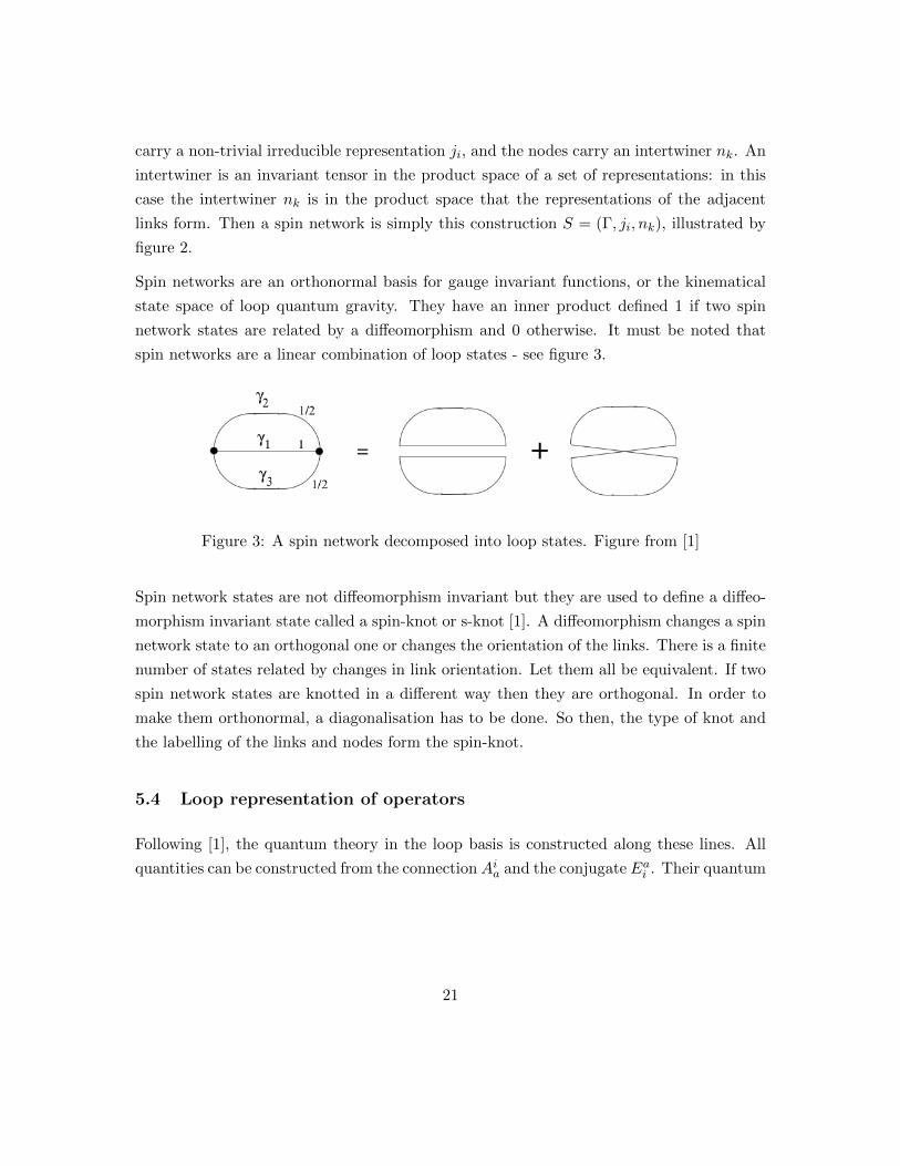
spin networks are a linear combination of loop states - see figure 3.

Figure 3: A spin network decomposed into loop states. Figure from [1]

Spin network states are not diffeomorphism invariant but they are used to define a diffeo-

morphism invariant state called a spin-knot or s-knot [1]. A diffeomorphism changes a spin

network state to an orthogonal one or changes the orientation of the links. There is a finite

number of states related by changes in link orientation. Let them all be equivalent. If two

spin network states are knotted in a different way then they are orthogonal. In order to

make them orthonormal, a diagonalisation has to be done. So then, the type of knot and

the labelling of the links and nodes form the spin-knot.

5.4 Loop representation of operators

Following [1], the quantum theory in the loop basis is constructed along these lines. All

quantities can be constructed from the connectionAia and the conjugate Eai . Their quantum

21

equivalents are defined on the functionals or states Ψ[A] as [1]

AiaΨ[A] = AiaΨ[A],

1

8πGEai Ψ[A] = −i~ δ

δAiaΨ[A].

(55)

In other words the action of A on a state is simply multiplication and the conjugate is a

functional derivative. The factor 18πG can be set to one. Notice that the right hand sides

do not live in the same space as Ψ[A] so use holonomies as the operators instead of A and

E [1].

The connection can be replaced by the holonomy U(A, γ) (46). Then the action of the

holonomy on the state Ψ is multiplication. The momentum E requires a bit more work and

in fact the action of E is to pick out intersections of the holonomy with a two-dimensional

surface:

Ei(S)U(A, γ) = ±i~U(A, γ1)τiU(A, γ2) (56)

i.e. E on a holonomy is equivalent to inserting a matrix ±i~τi where E and the holonomy

curve intersect. The holonomy γ is then split into γ1 and γ2. This comes from the fact

that E can be rewritten in smeared over a two-dimensional plane as

Ei(S) ≡ −i~∫S

dσ1dσ2εabc∂xb(σ)

∂σ1

∂xc(σ)

∂σ2(57)

where σ are coordinates on the two-dimensional surface. The derivative of U by A is given

byδ

δAia(x)U(A, γ) =

∫dsγa(s)δ3(γ(s)x)[U(A, γ1)τiU(A, γ2)] (58)

with γ1 and γ2 being the two parts into which the point s separates the curve γ and τ the

Pauli matrices [1].

The operators Tr(U) (a closed loop) and E give the unique representation, the loop repre-

sentation, of a quantised diffeomorphism invariant theory. This is the LOST theorem (for

Lewandowski, Okolow, Sahlmann and Thiemann) [23].

Equation (58) is crucial in what comes next. It turns out that the area of any physical sur-

face is quantised. This is the main result of loop quantum gravity: spacetime is quantised.

The area and volume operators were first defined by Rovelli and Smolin in [24] and the

22

first results of the disrcetisation of space were presented in this paper, later corrected by

Loll [25]. The full spectrum of the area and volume operators was calculated by Ashtekar

and Lewandowski in [26]. The argument for the discreteness of the area operator goes as

follows.

The area of a 2d surface S in 3d space is given by

A =

∫S

dx1dx2√

det q2d, (59)

which using Ashtekar variables can be written as

A =

∫S

dx1dx2√E3i E

3i, (60)

where the i in E3i has been raised with −2Tr(τiτj). Then one could use 55 to quantise

but this would be troublesome with two E ∝ δδA and the square root. Instead, promote

AΣ to a quantum operator by smearing the triad as in (57). First observe that the gauge

dependent quantity

E2(S) ≡∑i

Ei(S)Ei(S) (61)

acts on a spin network state at the intersections. If there is only one intersection then the

action is to insert two matrices τ according to equation (56). As two τ ’s form the Casimir

operator j(j + 1)× 1 then

E2(S)|S〉 = ~2j(j + 1)|S〉. (62)

23

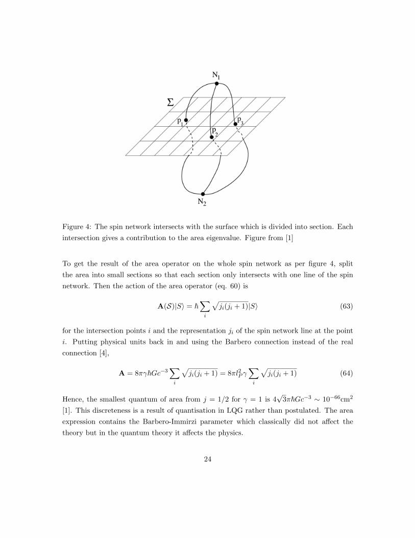
Figure 4: The spin network intersects with the surface which is divided into section. Each

intersection gives a contribution to the area eigenvalue. Figure from [1]

To get the result of the area operator on the whole spin network as per figure 4, split

the area into small sections so that each section only intersects with one line of the spin

network. Then the action of the area operator (eq. 60) is

A(S)|S〉 = ~∑i

√ji(ji + 1)|S〉 (63)

for the intersection points i and the representation ji of the spin network line at the point

i. Putting physical units back in and using the Barbero connection instead of the real

connection [4],

A = 8πγ~Gc−3∑i

√ji(ji + 1) = 8πl2Pγ

∑i

√ji(ji + 1) (64)

Hence, the smallest quantum of area from j = 1/2 for γ = 1 is 4√

3π~Gc−3 ∼ 10−66cm2

[1]. This discreteness is a result of quantisation in LQG rather than postulated. The area

expression contains the Barbero-Immirzi parameter which classically did not affect the

theory but in the quantum theory it affects the physics.

24

It was assumed in the treatment above that the spin network and area intersect only on

the links not the nodes. This allowed one to obtain the main part of the spectrum. If the

assumption is dropped then according to [26] one obtains the full spectrum

A(S) =4π~Gγc3

∑i

√2jui (jui + 1) + 2jdi (jdi + 1)− jti (jti + 1) (65)

where ji = (jui , jdi jti ) is the triplet at the intersection with a node. The intersections with

links are contained in this for jui = jdi .

It must be noted that the area operator and the volume operator below are not gauge-

invariant operators. Hence, they cannot be directly taken to represent physical quantities.

However, for certain reasons they are thought to imply that spacetime is discrete [27]:

Firstly, it is true that the area and volume operators have discrete spectra in any gauge. As

the discreteness depends on commutators of the operators and not the precise description

of the operators or observables, for any area the discreteness prevails. Also, discreteness

is independent of the dynamics of the system. This gives the basis for saying that LQG

predicts a discrete area and volume.

There is also a volume operator, of which there exist variants summarised in [28]. For a

full derivation of the quantum volume operator see [3]. Essentially the aim is to make the

following expression for the volume V for a region R into a quantum expression:

V(R) =

∫R

d3x√

detq =1

6

∫R

d3x√|εabcεijkEai EbjEck|. (66)

The volume operator only acts on nodes. More precisely the volume operator vanishes if

the region R does not contain a node of four or more spin network lines. The end result is

that the action of the volume operator on a spin network state is of the form

V(R)|Γ, jl, i1 . . . iN 〉 = (16π~γG)3/2∑n

V i′nin|Γ, jl, i1 . . . in . . . iN 〉, (67)

where |Γ, jl, i1 . . . iN 〉 = |s〉 is a spin network state (Γ graph, jl irreducible representations

labelling links and in intertwiners of nodes) and V i′nin

are matrices computed for some cases

in [29] and all cases included in [30]. These matrices depend on the nodes of the spin

network. The conclusion is that the volume operator has a discrete spectrum like the area

25

operator.

How can continuous smooth geometry arise from a quantised geometry? The concept of a

weave is the key to this understanding. Weaves were studied in [31] before the spin network

states and the discreteness of spacetime of loop quantum gravity were found. The quick

introduction below follows [1].

A 3d metric gab(x) = eia(x)eib(x) can be approximated by a spin network state for lengths

much larger than the Planck length. A spin network state is called a weave if it satis-

fiesV (R)|S〉 = (V [e,R] +O(lP /l))|S〉,A(S)|S〉 = (A[e,S] +O(lp/l))|S〉

(68)

with V [e,R] and A[e,S] denoting classical expressions of volume and area in terms of the

tetrad basis. This definition is not unique so physical space is a quantum superposition of

these weave states.

5.5 Quantisation of the Hamiltonian constraint

The Hamiltonian constraint was consistently quantised first by Thiemann in 1996 in [32].

The aim was to make a well-defined quantum Wheeler-DeWitt equation HΨ = 0. The

quantisation of the Hamiltonian constraint starts from the form of equation (35)

H(N) =

∫d3NV, AkcF kabεabc. (69)

To proceed with quantisation of the Hamiltonian constraint, introduce a path γx,u that

starts at point x with a tangent u and has length ε [1]. Then the holonomy can be written

as

hγx,u = 1 + εuaAa(x) +O(ε2). (70)

For a closed triangular loop αx,uv with two sides of length ε tangent to u, v

hαx,uv = 1 +1

2ε2uavbFab(x) +O(ε3). (71)

26

Then the Hamiltonian constraint (69) can be written as

H = limε→0

∫Nεijk Tr

(hγ−1

x,ukhαx,uiuj

V, hγx,uk)

d3x (72)

This can be promoted to a quantum operator since the holonomies can be directly pro-

moted and the volume operator was constructed earlier. The Poisson bracket becomes

a commutator. Since the volume operator acts only on nodes so does the Hamiltonian

constraint. To make the constraint covariant under diffeomorphisms and invariant under

internal gauge transformations the choice to make for x, ui, γ and α is given by the choices

in figure 5. The point x sits on a node n and the three tangents are along the links of the

spin network. If the node is four-valent or more, one must sum over all ordered permu-

tations of three links l, l′, l′′. In this case there is also ambiguity over position of the line

joining two of the tangents together. This ambiguity must be summed over, denoted by

label r. The end form of the quantum Hamiltonian constraint is then

H|S〉 = − i~

∑n,l,l′,l′′,r

Nnεl,l′,l′′Tr(hγ−1

xn,lhαr

xn,l′,l′′[V, hγxn,l

])|S〉. (73)

Figure 5: These are the definitions of the labels in the Hamiltonian operator 72. Figure

from [1].

The action of the Hamiltonian constraint on a node of a spin network state or more precisely

an s-knot state (diffeomorphism invariant spin network) is illustarated in figure 6 and

27

calculated exactly in [33]. It is possible to construct a Hamiltonian constraint with a

positive cosmological constant [34].

Figure 6: The Hamiltonian acts by adding a line and changing the representations labelling

the links. Figure from [1]

5.6 Coupling to matter

While loop quantum gravity does not try to unify matter fields, it is natural to extend

the formalism for gravity to matter fields. All kinds of matter fields can be included. For

details, derivations and quantisation see [35]. In brief, the s-knot state gets new labels

from the Yang-Mills group and the Hamiltonian is a sum of contributions from all matter

fields. Hgravity is simply 69 and

HYM =1

2g2YM

√| detE|3

tr[EaEb]Tr[EaEb +BaBb],

HDirac =1

2√| detE|

Eai (iπτ iDaξ +Da(πτ iξ) +i

2Kiaπξ + complex conjugate),

HHiggs =1

2√| detE|

(p2 + tr[EaEb]Tr[(Daφ)(Dbφ)] + e2V (φ2)

),

(74)

with p conjugate to the scalar field φ , π momentum conjugate to the fermion field ξ and

E conjugate to and B curvature of the Yang-Mills potential. The trace tr is in SU(2) and

Tr in GYM. gYM is the Yang-Mills coupling constant and D is the covariant derivative for

SU(2)×GYM [1].

28

6 An application: loop cosmology

The aim of quantum cosmology is to combine general relativity and quantum mechanics

in order to understand the universe as a whole. Concentrating on cosmology rather than

a general theory of quantum gravity has benefits. Firstly, cosmological symmetries of

spacetime simplify calculations. Cosmology is also a good stage for investigating the full

theory of quantum gravity and for drawing conclusions for issues such as the problem

of time, producing dynamics from frozen formalisms and observables in a background

independent theory. As well as being a theoretical playing field, quantum cosmology is the

most experimentally accessible part of quantum gravity. A recent review on loop quantum

cosmology is [7].

While there are benefits to investigating quantum gravity in cosmological setups, there are

also limits. Since symmetries of cosmological spacetime reduce the number of degrees of

freedom, the question must be posed: does quantum cosmology portray the main features

of quantum gravity? The answer seems to be yes if the extra degrees of freedom are

integrated out rather than “frozen” and the construction of the cosmology has the relevant

features [7]. It must be emphasised that cosmological models are not an approximation of

the full theory but a truncation. Hence, the equivalence of the model to the full theory

can only be tested by making the model more complicated and investigating whether the

results from the simpler theory carry over.

Loop quantum cosmology is different from other quantum cosmologies by the effects of

the quantum geometry. Since the full theory of loop gravity has a discrete spacetime,

this is inherited in the more symmetric cosmology models. The discreteness creates a new

repulsive force which is present in high-energy regimes in Planck scales. This is the main

result of LQC so far. Quantisation of geometry has some major effects in the cosmology

context [1]:

1. Singularities are absent. The inverse scale factor a−1 that appears in the Freedman

equation is bounded. In a sense, the universe has a minumum size and the Big Bang

is well behaved.

2. The scale factor is quantised and along with it the volume of the universe is quantised

too.

29

3. Since the scale factor can be interpreted as a cosmological time parameter, the cos-

mological time is quantised and so the evolution is discrete. The Wheeler-DeWitt

equation is a difference equation as will be presented below.

4. There is inflation immediately after the Big Bang which is driven by the quantum

properties of the gravitational field.

Key questions of LQC are how close to the big bang is spacetime smooth? Are dynamical

equations well-behaved at the singularity? Was there a deterministically connected universe

before the Big Bang? Is there an emergent time variable, required by Hamiltonian theory,

which governs the evolution of other parameters?

6.1 Isotropic spacetime

This brief introduction to isotropic models follows the presentation in [6].

Isotropy reduces the phase space such that only one variable is free. The metric is

ds2 = −N(t)2dt2 + a(t)2

(1

1− kr2dr2 + r2dΩ2

)(75)

where the lapse function N(t) can be absorbed into proper time τ by dτ = N(t)dt, and k is

−1 0 or 1 for a negative, zero or positive curvature model respectively. Then the evolution

equation or Friedmann equation is(a

a

)2

+k

a2=

8πG

3a−3Hmatter(a). (76)

The model can be studied with Hamiltonian techniques using the Einstein-Hilbert ac-

tion

SEH =1

16πG

∫d3xR[g] (77)

where the Ricci scalar for the metric in question is

R = 6

(a

N2a+

a2

N2a2+

k

a2− a

a

N

N3

). (78)

30

Substituting this into the action and integrating by parts

S =V0

16πG

∫dtNa3R =

3V0

8πG

∫dtN

(−aa2

N2+ ka

)(79)

with the definition V0 =∫

Σ d3x. From this form of the action the momenta are

pa =∂L

∂a= − 3V0

4πG

aa

N, pN =

∂L

∂N= 0. (80)

Note that pN is not a degree of freedom but a Lagrange multiplier since N does not appear

in the action. N multiplies the Hamiltonian constaint in the action and varying with

respect to N forces the Hamiltonian constraint to zero.

The same can be expressed in terms of Ashtekar variables. In Ashtekar variables the

isotropic connection and triad are

Aia(x)dxa = cωi,

Eai∂

∂xa= pXi

(81)

where ωi are invariant one-forms and Xi are invariant vector fields. In flat space ωi = dxi

and Xi are derivatives [36]. These two numbers c and p describe the fields. They are

related to the variables used above by

c =1

2(k − γa)

|p| = a2.(82)

The Poisson bracket is

c, p =8πγG

3V0. (83)

A new property is that p can be either negative or positive, corresponding to two different

possible orientations of the triad. In order to remove the volume element V0 from the

Poisson bracket, the variables can be rescaled as

p = V2/3

0 p, c = V1/3

0 c, Γ = V1/3

0 Γ. (84)

31

Thus, the Hamiltonian constraint in isotropic Ashtekar variables is

H = − 3

8πG(γ−2(c− Γ)2 + Γ2)

√|p|+Hmatter(p) = 0. (85)

which is equivalent to the Friedmann equation.

All states can be constructed by acting on the ground state by the holonomy

hi(c) = exp(cτi) = cos(c/2) + 2τi sin(c/2). (86)

An orthonormal basis in this representation is given by [37]

〈c|n〉 =exp(inc/2)√

2 sin(c/2). (87)

for integer n.

There are classical singularities at p = 0 and a = 0 so the evolution equation with scalar

matter φ

Hφ(a, φ, pφ) =1

2|p|−3/2p2

φ + |p|3/2V (φ) (88)

is singular which means the classical theory is incomplete. As we will see the singularities

can be removed as a result of the quantisation process.

Quantisation can be attempted via DeWitt quantisation [38] where states are denoted

by ψ(a). The canonical variables act on this, the scale factor as multiplication and its

conjugate pa as derivative. This can be then used to form the Wheeler-DeWitt operator

that quantises the Hamiltonian constraint. However, the scale factor has a continuous

spectrum in this formalism while quantum gravity implies a discrete spectrum for the

volume. Also, the scale factor is unbounded because it appears as a−1. Therefore one

should start with the full quantisation and then increase the symmetry to isotropy.

6.2 Discrete scale factor

In loop quantum cosmology, unlike the Wheeler-DeWitt quantisation, the inverse scale

factor can in fact be quantised and be found to be finite and to have an upper bound [39].

Its quantisation proceeds as follows [36]. The same trick can be performed on a−1 as for

32

the volume operator in eq 34. One way to write a−1 is

a−1 =

(1

2πγGc, |p|3/4

)2

=

(1

3πγG

∑i

trj(τihi(c)hi(c)−1,√V )

)2 (89)

for j = 1/2 and trace in the fundamental representation. Now it is straightforward to

promote a−1 to a quantum operator since this expression contains holonomies and the

volume operator. They can be promoted to their quantum versions and the Poisson bracket

turned into a commutator so that for an eigenstate |n〉

a−1|n〉 =16

γ2l4P

(√V|n|/2 −

√V|n|/2−1

)2|n〉 (90)

with the volume eigenvalues on an eigenstate |n〉 [40]

V(|n|−1)/2 = (1

6γl2P )3/2

√(|n| − 1)|n|(|n|+ 1) (91)

The operator a−1 has an upper bound (a−1max) = 32(2−

√2)

3lPreaching the maximum at n = 2

[39]. In the classical limit lP → 0 the divergence reappears. For large volumes, i.e.

large eigenstates, quantum behaviour is very similar to classical behaviour. Figure 7 il-

lustrates the behaviour of the inverse scale factor eigenvalues compared to the classical

divergence.

33

22 Martin Bojowald and Hugo A. Morales-Tecotl

0

0.2

0.4

0.6

0.8

1

0 5 10 15 20 25 30

n

j=5j=10

Fig. 1. Two examples for eigenvalues of inverse scale factor operators with j = 5(+) and j = 10 (!), compared to the classical behavior (dashed) and the approxi-mations (30) [41].

2. The first point demonstrates that the classical behavior is modified atsmall volume, but one can see that it is approached rapidly for volumeslarger than the peak position. Thus, the quantization (28) has the correctclassical limit and is perfectly admissible.

3. While the first two points verify our optimistic expectations, there is alsoan unexpected feature. The classical divergence is not just cut o! at afinite value, the eigenvalues of the inverse scale factor drop o! when we goto smaller volume and are exactly zero for n = 0 (where the eigenvalue ofthe scale factor is also zero). This feature, which will be important later,is explained by the fact that the right hand side of (27) also includesa factor of sgn(p)2 since the absolute value of p appears in the Poissonbracket. Strictly speaking, we can only quantize sgn(p)2a!1, not just a!1

itself. Classically, we cannot distinguish between both expressions – bothare equally ill-defined for a = 0 and we would have to restrict to positivep. As it turns out, however, the expression with the sign does have well-defined quantizations, while the other one does not. Therefore, we haveto use the sign when quantizing expressions involving inverse powers of a,and it is responsible for pushing the eigenvalue of the inverse scale factorat n = 0 to zero.

4. As already indicated in (27), we can rewrite the classical expression inmany equivalent ways. Quantizations, however, will not necessarily bethe same. In particular, using a higher representation j != 1

2 in (27), theholonomies in a quantization will change n by amounts larger than one.In (28) we will then have volume eigenvalues not just with n"1 and n+1,but from n " 2j to n + 2j corresponding to the coupling rules of angular

Figure 7: Eigenvalues of the inverse scale factor (× and +), approximations solid lines and

classical divergent behaviour dashed line. Figure from [36]

6.3 Dynamics

In order to study the dynamics one must quantise the Hamiltonian constraint, which in

loop quantum cosmology becomes a difference equation [43], [44]:

(V|n+4|/2 − V|n+4|/2−1)eikψn+4(φ)− (2 + γ2k2)(V|n|/2 − V|n|/2−1)ψn(φ)

+ (V|n−4|/2−V|n−4|/2−1)e−ikψn−4(φ)

=− 8π

3Gγ3l2P Hmatter(n)ψn(φ)

(92)

It has this discrete structure since now due to the discreteness of the scale factor, time

can be interpreted as discrete too. The above equation is valid for k = 0 and k = 1 only.

In the classical limit, i.e. n 1 the discrete wavefunction can be appoximated smooth

and the difference equation may be Taylor expanded in powers of p/γl2P. This recovers the

34

classically quantised Wheeler-DeWitt equation

1

2

(4

9l4P∂2

∂p2− k)ψ(p, φ) = −8π

3GHmatter(p)ψ(p, φ). (93)

6.4 Removal of singularity

In the flat k = 0,Λ = 0 model there is no Big Bang but there is the Big Bounce [45]. One

can evolve the wavefunctions in the evolution equation (92) to negative time, or negative

n, so that there is evolution before the classical singularity at a = 0. This is because the

ψ0(φ) drops out of the equation since for n = 0, V|n|/2 − V|n|/2−1. Also Hmatter|n〉 = 0 so

ψ0(φ) is decoupled from all other values of ψ [36]. This can be seen in figure 8 where the

classical singular behaviour and the quantum bounce are pictured. 32

a) b)

-1.2

-1

-0.8

-0.6

-0.4

-0.2

0

0 1*104

2*104

3*104

4*104

5*104

v

!

-1.2

-1

-0.8

-0.6

-0.4

-0.2

0

0 1*104

2*104

3*104

4*104

5*104

v

!

quantumclassical

FIG. 2: a) Classical solutions in k=0, ! = 0 FRW models with a massless scalar field. Since

p(!) is a constant of motion, classical trajectories can be plotted in the v-! plane. There are two

classes of trajectories. In one the universe begins with a big-bang and expands and in the other it

contracts into a big-crunch. There is no transition between these two branches. Thus, in a given

solution, the universe is either eternally expanding or eternally contracting. b) LQC evolution.

Expectation values and dispersion of |v|!, are compared with the classical trajectory. Initially, the

wave function is sharply peaked at a point on the classical trajectory at which the density and

curvature are very low compared to the Planck scale. In the backward evolution, the quantum

evolution follows the classical solution at low densities and curvatures but undergoes a quantum

bounce at matter density " ! 0.41"Pl and joins on to the classical trajectory that was contracting

to the future. Thus the big-bang singularity is replaced by a quantum bounce.

in LQC. One can now explore physical consequences and compare them with those of theWDW theory.

Physics of this quantum dynamics was first studied in detail using computer simulations[53]. Recall that in the classical theory we have two types of solutions: those that start witha big-bang and expand forever and their time reversals which begin with zero density in thedistant past but collapse into a future, big-crunch singularity (see Fig.2(a)). The idea, as inthe WDW theory, was to start with a wave function which is sharply peaked at a point ofan expanding classical solution when the matter density and curvature are very small andevolve the solution backward and forward in the internal time defined by the scalar field !.As in the WDW theory, in the forward evolution, the wave function remains sharply peakedon the classical trajectory. Thus, as in the WDW theory, LQC has good infrared behavior.However, in the backward evolution, the expectation value of the volume operator deviatesfrom the classical trajectory once the matter density is in the range 10!2 to 10!3 times thePlanck density. Instead of following the classical solution into singularity, the expectationvalue of volume bounces and soon joins a classical solution which is expanding to the future.Thus, the big-bang is replaced by a quantum bounce. Furthermore, the matter density atwhich the bounce occurs is universal in this model: it given by "max " 0.41"Pl independentlyof the choice of state (so long as it is initially semi-classical in the sense specified above).

The fact that the theory has a good infrared as well as ultraviolet behaviors is highly non-trivial. As we saw, the WDW theory fails to have good ultraviolet behavior. Reciprocally,

Figure 8: a) Singular behaviour in classical models with k = 0,Λ = 0 flat model with a

massless scalar field. b) In LQC there is bounce [45] at matter density ρ ∼ 0.41ρPlanck.

Figure from [7]

6.5 Inflation

Inflation can be realised classically by introducing a state parameter ω and setting it to

ω < −13 . Then the energy density to be used in the Friedmann equation is

ρ(a) ∝ a−3(ω+1) (94)

35

and the solutions of the Friedmann equation fall into the following categories

a(t) ∝

(t− t0)2/(3ω+3) for − 1 < ω < −1

3 (power-law inflation),

exp(√

Λt) for ω = −1 (standard inflation),

(t0 − t)2/(3ω+3) for ω < −1 (super-inflation).

(95)

In quantum theory, the Friedmann equation is modified since the inverse scale factor is

bounded. The boundedness of a−1 can be absorbed into the classical equations of motion

by replacing a−3 with dj(a) = a−3p(3a2/jγl6P). Then the effective scalar energy density

is

ρeff(a) =1

2xal(a)−3l

−l(a)−3P p2

φW (φ), (96)

where x and l have some dependence on quantisation ambiguities. For a usual quantisation

the effective ω is then less than -1 [36] so LQC predicts that there is super-inflation in the

initial stage of the universe [41]. This is true for any matter. In addition, the inflation ends

when the modified energy density starts to decrease [36]. This is a major result of LQC:

early universe inflation is predicted and also ended by loop quantum effects.

7 Black hole entropy

Loop quantum gravity provides a way of calculating the entropy of a black hole. It turns

out that compared to the semiclassical Hawking-Bekenstein entropy formula there is a

logarithmic quantum correction to the entropy of a black hole [46]. Before discussing the

loop treatment of black holes, the classical theory will be discussed in order to motivate

the search for a quantum description of black hole entropy.

All stationary black holes can be described by three parameters, mass M , charge Q and

angular momentum J according to the famous no-hair theorem. Space near a black hole

with angular momentum and charge is given by the Kerr-Newman solution of Einstein’s

equations,

c2ds2 = −(dr2

∆+ dθ2

)ρ2 +

(cdt− αsin2θdφ

)2 ∆

ρ2−((r2 + α2)dφ− αcdt

) sin2θ

ρ2(97)

36

which is in spherical coordinates and α, ρ and ∆ are the following:

α =J

Mc,

ρ2 = r2 + α2cos2θ,

∆ = r2 − 2GM

c2r + α2 +

Q2G

4πε0c4.

(98)

The energy of the black hole can be reduced but only to a finite minimum [47]. On the

other hand, Hawking proved that the area of a black hole cannot be decrease [48] and

interestingly the area of a black hole horizon is given by the irreducible mass,

A = 16πM2irr. (99)

Hawking’s area theorem inspired Bekenstein to make a connection between entropy and

the area of a black hole [49]. The Bekenstein-Hawking entropy of a black hole is

SBH =kBA

4l2P. (100)

It was argued that since the mass of a Schwarzschild black hole is given by

M =

√A

16πG2, (101)

the thermodynamical equation T−1 = dSdE should imply that there is a black hole temper-

ature. Hawking proved that black holes in fact emit thermal Hawking radiation [50] by

considering quantum fields near the horizon. For example for a Schwarzschild black hole

the Hawking temperature is

T =~c3

8πGMkB. (102)

Hawking radiation is essentially due to a stationary observer near the black hole being

non-inertial. This causes the observer to see a different vacuum compared to an inertial

observer’s vacuum that is usually used as the definition of a vacuum.

Using the Hawking temperature to compute the thermodynamic entropy and comparing

it with the Bekenstein-Hawking entropy, it can be argued that the entropy of a black hole

is not given by the entropy of the mass of the black hole only [4]. This is a motivation for

37

the search of a quantum description of black hole entropy.

Besides the entropy there is another motivation for finding a full quantum description

of black holes. It is the fact that the black hole becomes smaller as it radiates and the

curvature near the horizon increases [4]. As the curvature increases the semiclassical picture

no longer holds and contradictions arise. An example is the information paradox which

asks where does the information trapped in the black hole go as the black hole radiates

and decreases in size.

Loop quantum gravity is the only quantum theory of gravity which has managed to repro-

duce the Bekenstein-Hawking formula for many types of black hole; string theory can be

used only to solve extremal or near extremal black holes [1]. Black hole entropy has been

investigated in the loop quantum gravity context e.g. in [51]. Most black hole calculations

assume that the black hole is large compared to the Planck scale and all ignore Hawking

radiation completely [4]. The study of black holes in loop quantum gravity is essentially the

study of the interaction between the horizon and the lines of the spin network puncturing

the horizon.

The simplest and most thoroughly studied case is the isolated spherical black hole which

does not interact with the outside space. Classically any black hole without charge and

angular momentum evolves to a Schwarzschild black hole. In quantum theory, however, the

Heisenberg uncertainty principle forbids a black hole from being exactly Schwarzschild. The

thermal fluctuations in the matter distribution inside the black hole cause inhomogeneities

in the gravitational field. These little fluctuations can be ignored [4].

The microstates Ni of the black hole are complicated but they are needed to calculate the

entropy S = kB log(Ni). There is a major simplification, however, in that the ensemble of

microstates required contains only the states of the horizon [1]. This is because a statistical

ensemble is defined as the phase space of energy exchanges, which for black holes correspond

to changes in the area. Hence, entropy is a function of the area.

First consider the definition of an isolated horizon. There are two conditions for an isolated

horizon [4]. Consired the spin connection Γia defined in the space-time. Denote the pullback

of a quantity with a bar. Then define an Abelian connection Wa = −Γiari on the boundary

S, with ri vector. Using a definition of an antisymmetric tensor Σiabε

abc ≡ Eci one can

38

state that the first condition that an isolated horizon satisfies is [52]

∂aWb − ∂bWa = −2γΣiabri. (103)

Secondly, the lapse must vanish for the boundary so that the Hamiltonian constraint does

not generate evolution across the boundary.

For calculating the entropy of a spherical black hole, one must count the number of quantum

states with the eigenvalue of the area in an infinitesimal range around the black hole area

A0. If a line of a spin network with value jI punctures the black hole horizon it creates

an area A = 8πγl2P√jI(jI + 1) as is familiar from eq. 64. There is also a contribution

from Σab which is the E3 operator with eigenvalues m ranging from −jI ≤ mI ≤ jI with

a condition∑

I mI = 0. Including diffeomorphism invariance and all these conditions the

Bekenstein-Hawking formula is recovered with a logarithmic correction [46]:

S(A) =A

4l2P− 3

2log

a

l2P+O(1) + . . . (104)

This is an important result since to get this form of the entropy, a particular value for the

Barbero-Immirzi parameter must be assumed. The value assumed is from [53], from the

solution of the equation

1 =

∞∑k=1

(k + 1) exp

(−1

2γ√k(k + 2)

). (105)

The solution is γ ≈ 0.2375. It seems dissatisfactory to have to determine a value for γ.

However, consistency with the Bekenstein-Hawking formula for several types of black holes

including charge, matter or a cosmological constant can be seen to require this value of γ

(see [54] and references therein).

The exact value of the Immirzi parameter is still the target of discussion (e.g. [55]). In

particular, the current agreement is that

Sloop =1

4

γ

γ0

A

~G(106)

with the most updated value [56, 57] of γ = γ0 = 0.274076... It is not understood why the

Immirzi parameter must have this particular value and why it should be cancelled.

39

8 Spinfoam formalism

In ordinary quantum mechanics there are several equivalent formulations, the Schrodinger

and Heisenberg pictures and the path integral formalism. Similarly, the Hamiltonian for-

malism of loop quantum gravity has an alternative called spinfoam formalism. It is a

sum-over-histories approach to calculating transition amplitudes of spin network states.

The question it aims to answer is what is the transition probability from an initial geome-

try on a 3d slice to a final geometry. This presentation follows [1]. An introduction to the

topic is in [8].

The path integral which measures the transition amplitude and that the theory aims to

define is of the form ∫D[gµν(x)]eiSGR[g] (107)

with D being the integration measure which covers all possible metrics [1]. However, it is

not known what a non-perturbative integration measure looks like. But the discreteness

of space in LQG allows another approach - the sum-over-histories formalism is found from

spin networks. Interestingly, several different approaches all lead to the same spinfoam

formalism of nonperturbative quantum gravity [1].

The spinfoam formalism was first developed in [58] and in [59]. The key element of the

formalism is that instead of an integral, the transition amplitude is given by a sum-over-

histories of spin networks. This is where the concept of a spinfoam comes in. A spin foam

is a history of spin networks defined as follows. Essentially it is a worldsurface that a spin

network sweeps out as a “time”-variable progresses.

In more detail a spinfoam consists of vertices swept out by nodes, edges swept out by

links and additionally faces where nodes branch. This is a two-complex structure and it is

illustrated in figure 11. A spinfoam has the additional structure that the edges inherit the

representation labelling the links and the vertices have the intertwiners from the nodes as

labels. It is important to note that a spinfoam is background independent and is defined

without reference to a spacetime.

40

Figure 9: The action of a Hamiltonian is on a node, for example adding lines like this. [1]

Figure 10: A vertex of a spinfoam caused by the action of the Hamiltonian [1]

p

s

fs

i

f

i!

!

q

p

5

5

f

i

6

7

8

8

1

3

7

63

3

s

1

sf

i

s

!

!

Figure 11: A spinfoam with two vertices. si and sf label the initial and final spin network

states. p and q label the vertices. [1]

41

Formally, a spinfoam W is a sum over amplitudes A(σ)

W (s, s′) =∑σ

A(σ), A(σ) =∏v

Av(σ) (108)

where s is the initial spin network state and s′ is the final spin network state and a single

step in the evolution is

Av(σ) = 〈sn+1|e−∫d3H(x)dt|sn〉. (109)

For small dt, one can discard higher-order terms in H so that only the linear action of H

remains. H acts on the nodes adding lines for example like in figure 11. The action of H

is the origin of the vertices in a spinfoam.

A spinfoam model is then defined by the set of two-complexes and weights associated to

them, the set of representations and intertwiners, and vertex and edge amplitudes added

to the vertices and edges. The most recent spinfoam model is built on a chain of theories

of increasing complexity. Mostly the theories are euclidean but the later versions can

be made lorentzian [1]. In brief, the first attempt was the Ponzano-Regge model [60]

which discretises 3d space with triangles. It comes with infrared divergences so further

developments were required. The Ponzano-Regge model has a generalisation to 4d by

the Ooguri model. The Ooguri model uses BF-theory1 instead of GR to help simplify

calculations. The next version, the Barrett-Crane model, includes local degrees of freedom

so it allows to implement GR in the form of constraints. Then a possible way to implement

the two-complexes is for example group field theory [61].

Most new developments in loop quantum gravity come via this formalism. Like with ordi-

nary quantum mechanics, different formulations are useful for different types of calculation

and the case is the same in loop quantum gravity. The spinfoam formalism should be

equivalent to the Hamiltonian formalism, however, this has only been rigorously proved in

3d in [62].

The question is what can be done with the spinfoam formalism. The amplitudes it allows

one to calculate relate to physical measurements via the area and volume operators. Since

spin networks are eigenvalues of the area and volume operators, they should in principle

give results of measuring 3d surface geometry [1]. One can also compute the Minkowski

vacuum via it [63].

1For an SO(4) two-form BIJ and connection ωIJ , S[B,ω] =∫BIJ ∧ F IJ [ω].

42

A major result is that spinfoams can be used to calculate n-point functions, which have

been defined [64] for loop quantum gravity. The n-point functions can be used to find the

graviton propagator or in other words Newton’s law without space and time [65]. There is

increasing use of spin foam formalism in loop quantum cosmology too [66]

9 Some open problems

Loop quantum gravity has managed to surprise its investigators with its properties. Quan-

tisation of the area and volume was not expected and neither was the resolution of the

Big Bang. Success came in the form of a coherent combination of general relativity with

quantum mechanics without further assumptions. On the way problems have been solved

such as the overcompleteness of the loop basis and the need of producing background de-

pendent quantities from a background independent theory [67]. Several parts of the theory,

however require further research as the theory is promising but still incomplete.

There is lack of experimental evidence. This is a problem plaguing theoretical physics in

general and quantum gravity is not an exception. There is not a straightforward prediction

that the theory makes which could be experimentally tested, though the theory does make

predictions such as the quantisation of area.

Loop gravity phenomenology is in general a developing area. This is because the full loop

quantum gravity does not provide a derivation of the phenomenological assumptions [69].

A few active directions of research exist: one is the possible Lorentz violation. There is a

potential description of this in the form of doubly special relativity where the Planck energy

is invariant like the speed of light [70]. For an introduction to the topic see [71].

The idea behind the claim that Lorentz invariance might be violated is easy to understand.

Broken Lorentz invariance seems inevitable since space-time is discrete at the Planck scale

and there are possible consequences for light dispersion relations. These deviations may

be observable in gamma ray bursts in cosmology [72].

A recent claim by Bojowald is that loop gravity can be tested via the inverse tetrad

corrections [73]. There are several types of issue to be solved in loop quantum gravity.

Investigation needs to be done on the dynamics of inhomogeneous models, the relationship

between cosmological models and full quantum gravity and derivation of effective equations

43

for inhomogeneous models [6].

On the application to loop quantum cosmology, as was discussed in section 6, it is unclear

whether the singularity resolved in the symmetric case is a property of the full theory. It

is possible that even if it is resolved in simple cases, in cases with inhomogeneous matter

and other degrees of freedom the singularity returns.

Black hole entropy calculations have been done numerically without the usual assumption

of a large area. There are results in [68] which are not yet understood. Therefore, more

needs to be done in the black hole direction too.

Rovelli [1] suggests that despite the theory having no ultraviolet divergences there might

be infrared divergences. Ultraviolet finiteness can be shown in different ways but for

large j there might be infrared divergences [67]. A possible strategy for removing infrared

divergences is under investigation [74, 75].

The recovery of the correct classical limit has not been confirmed. A proof has not been

found to confirm that general relativity is recovered in the low-energy limit. However, the

degrees of freedom and general covariance match general relativity and calculations with

n-point functions are successful [67].

The spinfoam formalism needs to be applied further. Parts of the theory have not been

solved yet, such as higher order n-point functions.

As well as these areas which require further investigation there is criticism of the existing

parts of the theory, most notably argued in [77]. The arguments have been rebutted by

Thiemann in [69]. One criticism was that LQG does not reproduce the harmonic oscillator

since p and q, the usual variables, are not defined in the loop representation. It is shown

in [69] however, that there is a set of observables with energy expectation values n~ like

for the harmonic oscillator.

There was also criticism of the ambiguities in constructing the Hamiltonian constraint.

There are factor ordering ambiguities and freedom of the choice of representation for the

holonomies. The factor ordering ambiguity can be removed by demanding a natural result.

The choice was whether to put tetrads to the left or right of the holonomies. If the

holonomy acts on an arbitrary point of a spin network line so that it produces a vertex,

there is a problem. Then the tetrads, or the volume operator that they form, will give

a contribution for that vertex when, to start with, there was no vertex [4]. This in the

44

limit of the triangulation going to zero will cause a divergence of the Hamiltonian. Another

ambiguity was that the holonomy was chosen to be in the fundamental representation when

in fact it could have been in any representation. The criticism of these ambiguities has

been discussed in [76].

Related to the Hamiltonian constraint is the constraint algebra which has been under mi-

croscope too. It was argued that the constraint algebra does not close off-shell, in particular

for two Hamiltonian constraints [77]. This problem is still unanswered, however, attempts

are being made with the Master constraint programme [78]. The Master constraint pro-

gramme combines the diffeomorphism constraint and the Hamiltonian constraint into one,

and the correct classical limit of the algebra has been recovered in Algebraic quantum

gravity [79].

It has also been shown that standard model matter couplings can be included easily in

LQG. The coupling does not lead to anomalies or divergences. The question is the absence

of consistency requirements on the matter couplings at the kinematical level. Will there

be consistency requirements for the matter in the dynamical or semiclassical limit?

10 Conclusion

Loop quantum gravity is a nonperturbative background independent formulation of quan-

tised general relativity. It builds on the Hamiltonian formalism of general relativity where

four-dimensional spacetime is split into three-dimensional spatial slices and a time direc-

tion. The action of general relativity has constraints. These constraints can be expressed

neatly in terms of the Ashtekar variables which use an SU(2) connection and its momen-

tum conjugate. This introduces a variable called the Barbero-Immirzi parameter which

has an important role in the quantum theory.

A basis of solutions for the constraints are the Wilson loops. These can be developed

further to define the spin network basis which is a complete basis for the quantum theory.

Using the spin network basis, the system of constraints can be quantised. It is found

that the area and volume operators of loop quantum gravity have discrete eigenvalues,

which implies that spacetime is quantised. The size of the quanta are of Planck scale and

proportional to the Immirzi parameter. This dicreteness of space is the reason why loop

quantum gravity is UV divergence free.

45

The quantisation of spacetime has interesting consequences in the context of cosmology.

Loop quantum cosmology is a truncated version of the full loop quantum gravity theory

and the exact relationship between loop cosmology and the full theory is still under inves-

tigation. However, the result that spacetime is quantised implies at least for the FLRW

model and homogeneous cosmology models that singularities are resolved. The Big Bang is

replaced by the Big Bounce where the classical singularity is avoided due to the loop quan-

tum gravity effects. Early universe inflation is automatically predicted and later stopped

by loop quantum cosmology. Loop cosmology is a rapidly developing area where current

research aims to consider models of increasing complexity to see whether results from sim-

pler models carry over. In particular, interacting matter and inhomogeneities cannot be

analysed using current methods.

Another application of loop quantum gravity is the black hole entropy calculation which

fixes the value of the Immirzi parameter. More recent developments of loop quantum

gravity have been created in the spinfoam formalism which is a path integral formulation

of loop quantum gravity. Most importantly, this formalism allows the calculation of n-point

functions and the graviton propagator. There is much work to do in the topic of n-point

functions because it is a very recently founded topic in loop quantum gravity.

Loop quantum gravity is a theory that is attacting more research currently because of

the number of possible investigation lines for researchers. Still, with only about a hundred

researchers working on it worldwide it has to answer to criticism from the vast string theory

community who are the main competitors in search for a quantum theory of gravity. While

loop quantum gravity does not attempt to unify matter and gravity it can incorporate

matter easily. The theory makes predictions and stands on a rigorous foundation, which

cannot be said of string theory. However, it has not been proved that general relativity is

the low-energy limit of loop quantum gravity, nor has a choice been made of the best way

to define a Lorentzian version of the theory. Hopefully these questions will be answered by

the community in the future.

46

References

[1] C. Rovelli, “Quantum gravity,” Cambridge, UK: Univ. Pr. (2004) 455 p

[2] R. Gambini and J. Pullin, “Loops, knots, gauge theories and quantum gravity,” Cam-

bridge, UK: Univ. Pr. (1996) 321 p

[3] T. Thiemann, “Modern canonical quantum general relativity,” Cambridge, UK: Cam-

bridge Univ. Pr. (2007) 819 p [gr-qc/0110034].

[4] R. Gambini and J. Pullin, “A first course in loop quantum gravity,” Oxford, UK: Univ.

Pr. (2011) 183 p

[5] L. Smolin, “Three roads to quantum gravity,” London, UK: Weidenfeld & Nicolson

(2000) 231 p

[6] M. Bojowald, “Loop quantum cosmology,” Living Rev. Rel. 11, 4 (2008).

[7] A. Ashtekar and P. Singh, “Loop Quantum Cosmology: A Status Report,” Class.

Quant. Grav. 28, 213001 (2011) [arXiv:1108.0893 [gr-qc]].

[8] J. C. Baez, “An Introduction to spin foam models of quantum gravity and BF theory,”

Lect. Notes Phys. 543, 25 (2000) [gr-qc/9905087].

[9] R. M. Wald, Chicago, Usa: Univ. Pr. ( 1984) 491p

[10] R. Arnowitt, S. Deser, C. Misner, in “Gravitation: an introduction to current re-

search”, editor L. Witten, Wiley, New York (1962) pp. 227265.

[11] A. Ashtekar, “New Variables for Classical and Quantum Gravity,” Phys. Rev. Lett.

57, 2244 (1986).

[12] G. Immirzi, “Quantum gravity and Regge calculus,” Nucl. Phys. Proc. Suppl. 57, 65

(1997) [gr-qc/9701052].

[13] A. Ashtekar, “New Variables for Classical and Quantum Gravity,” Phys. Rev. Lett.

57, 2244 (1986).

[14] A. Ashtekar, “New Hamiltonian Formulation of General Relativity,” Phys. Rev. D 36,

1587 (1987).

47

[15] T. Thiemann, “Anomaly - free formulation of nonperturbative, four-dimensional

Lorentzian quantum gravity,” Phys. Lett. B 380, 257 (1996) [gr-qc/9606088].

[16] J. F. Barbero G., “Real Ashtekar variables for Lorentzian signature space times,”

Phys. Rev. D 51, 5507 (1995) [gr-qc/9410014].

[17] R. Giles, “The Reconstruction Of Gauge Potentials From Wilson Loops,” Phys. Rev.

D 24, 2160 (1981).

[18] S. Mandelstam, “Feynman rules for electromagnetic and Yang-Mills fields from the

gauge independent field theoretic formalism,” Phys. Rev. 175, 1580 (1968).

[19] T. Jacobson and L. Smolin, “Nonperturbative Quantum Geometries,” Nucl. Phys. B

299, 295 (1988).

[20] C. Rovelli and L. Smolin, “Loop Space Representation of Quantum General Relativ-

ity,” Nucl. Phys. B 331, 80 (1990).

[21] C. Rovelli and L. Smolin, “Knot Theory and Quantum Gravity,” Phys. Rev. Lett. 61,

1155 (1988).

[22] C. Rovelli and L. Smolin, “Spin networks and quantum gravity,” Phys. Rev. D 52,

5743 (1995) [gr-qc/9505006].

[23] J. Lewandowski, A. Okolow, H. Sahlmann and T. Thiemann, “Uniqueness of diffeo-

morphism invariant states on holonomy-flux algebras,” Commun. Math. Phys. 267, 703

(2006) [gr-qc/0504147].

[24] C. Rovelli and L. Smolin, “Discreteness of area and volume in quantum gravity,” Nucl.

Phys. B 442, 593 (1995) [Erratum-ibid. B 456, 753 (1995)] [gr-qc/9411005].

[25] R. Loll, “Spectrum of the volume operator in quantum gravity,” Nucl. Phys. B 460,

143 (1996) [gr-qc/9511030].

[26] A. Ashtekar and J. Lewandowski, “Quantum theory of geometry. 1: Area operators,”

Class. Quant. Grav. 14, A55 (1997) [gr-qc/9602046].

A. Ashtekar and J. Lewandowski, “Quantum theory of geometry. 2. Volume operators,”

Adv. Theor. Math. Phys. 1, 388 (1998) [gr-qc/9711031].

[27] C. Rovelli, “Loop quantum gravity,” Living Rev. Rel. 11, 5 (2008).

48

[28] J. Lewandowski, “Volume and quantizations,” Class. Quant. Grav. 14, 71 (1997) [gr-

qc/9602035].

[29] R. De Pietri and C. Rovelli, “Geometry eigenvalues and scalar product from recoupling

theory in loop quantum gravity,” Phys. Rev. D 54, 2664 (1996) [gr-qc/9602023].

[30] T. Thiemann, “Closed formula for the matrix elements of the volume operator in

canonical quantum gravity,” J. Math. Phys. 39, 3347 (1998) [gr-qc/9606091].

[31] A. Ashtekar, C. Rovelli and L. Smolin, “Weaving a classical geometry with quantum

threads,” Phys. Rev. Lett. 69, 237 (1992) [hep-th/9203079].

[32] T. Thiemann, “Quantum spin dynamics (QSD),” Class. Quant. Grav. 15, 839 (1998)

[gr-qc/9606089].

[33] R. Borissov, R. De Pietri and C. Rovelli, “Matrix elements of Thiemann’s Hamilto-

nian constraint in loop quantum gravity,” Class. Quant. Grav. 14, 2793 (1997) [gr-

qc/9703090].

[34] L. Smolin, “Quantum gravity with a positive cosmological constant,” hep-th/0209079.

[35] T. Thiemann, “QSD 5: Quantum gravity as the natural regulator of matter quantum

field theories,” Class. Quant. Grav. 15, 1281 (1998) [gr-qc/9705019].

[36] M. Bojowald and H. A. Morales-Tecotl, “Cosmological applications of loop quantum

gravity,” Lect. Notes Phys. 646, 421 (2004) [gr-qc/0306008].

[37] M. Bojowald, “Quantization ambiguities in isotropic quantum geometry,” Class.

Quant. Grav. 19, 5113 (2002) [gr-qc/0206053].

[38] B. S. DeWitt, “Quantum Theory of Gravity. 1. The Canonical Theory,” Phys. Rev.

160, 1113 (1967).

[39] M. Bojowald, “The Inverse scale factor in isotropic quantum geometry,” Phys. Rev.

D 64, 084018 (2001) [gr-qc/0105067].

[40] M. Bojowald, “Loop quantum cosmology. II. Volume operators,” Class. Quant. Grav.

17, 1509 (2000) [gr-qc/9910104].

[41] M. Bojowald, “Inflation from quantum geometry,” Phys. Rev. Lett. 89, 261301 (2002)

[gr-qc/0206054].

49

[42] C. W. Misner, “The Isotropy of the universe,” Astrophys. J. 151, 431 (1968).

[43] M. Bojowald, “Isotropic loop quantum cosmology,” Class. Quant. Grav. 19, 2717

(2002) [gr-qc/0202077].

[44] M. Bojowald and K. Vandersloot, “Loop quantum cosmology, boundary proposals,

and inflation,” Phys. Rev. D 67, 124023 (2003) [gr-qc/0303072].

[45] M. Bojowald, “Absence of singularity in loop quantum cosmology,” Phys. Rev. Lett.

86, 5227 (2001) [gr-qc/0102069].

[46] R. K. Kaul and P. Majumdar, “Logarithmic correction to the Bekenstein-Hawking

entropy,” Phys. Rev. Lett. 84, 5255 (2000) [gr-qc/0002040].

[47] D. Christodoulou and R. Ruffini, “Reversible transformations of a charged black hole,”

Phys. Rev. D 4, 3552 (1971).

[48] S. W. Hawking, “Gravitational radiation from colliding black holes,” Phys. Rev. Lett.

26, 1344 (1971).

[49] J. D. Bekenstein, “Black holes and entropy,” Phys. Rev. D 7, 2333 (1973).

[50] S. W. Hawking, “Particle Creation by Black Holes,” Commun. Math. Phys. 43, 199

(1975) [Erratum-ibid. 46, 206 (1976)].

[51] C. Rovelli, Phys. Rev. Lett. 77, 3288 (1996) [gr-qc/9603063].

[52] A. Ashtekar and B. Krishnan, “Isolated and dynamical horizons and their applica-

tions,” Living Rev. Rel. 7, 10 (2004) [gr-qc/0407042].

[53] K. A. Meissner, “Black hole entropy in loop quantum gravity,” Class. Quant. Grav.

21, 5245 (2004) [gr-qc/0407052].

[54] A. Corichi, “Black holes and entropy in loop quantum gravity: An Overview,”

arXiv:0901.1302 [gr-qc].

[55] J. Engle, K. Noui, A. Perez and D. Pranzetti, “Black hole entropy from an SU(2)-

invariant formulation of Type I isolated horizons,” Phys. Rev. D 82, 044050 (2010)

[arXiv:1006.0634 [gr-qc]].

[56] A. Ghosh and P. Mitra, “An Improved lower bound on black hole entropy in the

quantum geometry approach,” Phys. Lett. B 616, 114 (2005) [gr-qc/0411035].

50

[57] I. Agullo, G. J. Fernando Barbero, E. F. Borja, J. Diaz-Polo and E. J. S. Villasenor,

“The Combinatorics of the SU(2) black hole entropy in loop quantum gravity,” Phys.

Rev. D 80, 084006 (2009) [arXiv:0906.4529 [gr-qc]].

[58] J. C. Baez, “Spin foam models,” Class. Quant. Grav. 15, 1827 (1998) [gr-qc/9709052].

[59] M. PReisenberger and C. Rovelli, “’Sum over surfaces’ form of loop quantum gravity,”

Phys. Rev. D 56, 3490 (1997) [gr-qc/9612035].

[60] L. Freidel, Nucl. Phys. Proc. Suppl. 88, 237 (2000) [gr-qc/0102098].

[61] A. Perez and C. Rovelli, Phys. Rev. D 63, 041501 (2001) [gr-qc/0009021].

[62] K. Noui and A. Perez, “Three-dimensional loop quantum gravity: Physical scalar

product and spin foam models,” Class. Quant. Grav. 22, 1739 (2005) [gr-qc/0402110].

[63] F. Conrady, L. Doplicher, R. Oeckl, C. Rovelli and M. Testa, Phys. Rev. D 69, 064019

(2004) [gr-qc/0307118].

[64] L. Modesto and C. Rovelli, “Particle scattering in loop quantum gravity,” Phys. Rev.

Lett. 95, 191301 (2005) [gr-qc/0502036].

[65] C. Rovelli, “Graviton propagator from background-independent quantum gravity,”

Phys. Rev. Lett. 97, 151301 (2006) [gr-qc/0508124]. E. Bianchi, L. Modesto, C. Rovelli

and S. Speziale, “Graviton propagator in loop quantum gravity,” Class. Quant. Grav.

23, 6989 (2006) [gr-qc/0604044].

[66] E. Bianchi, C. Rovelli and F. Vidotto, “Towards Spinfoam Cosmology,” Phys. Rev. D

82, 084035 (2010) [arXiv:1003.3483 [gr-qc]].

[67] C. Rovelli, “Loop quantum gravity: the first twenty five years,” Class. Quant. Grav.

28, 153002 (2011)

[68] A. Corichi, J. Diaz-Polo and E. Fernandez-Borja, Phys. Rev. Lett. 98, 181301 (2007)

[gr-qc/0609122].

[69] T. Thiemann, “Loop Quantum Gravity: An Inside View,” Lect. Notes Phys. 721, 185

(2007) [hep-th/0608210].

[70] J. Magueijo and L. Smolin, “Generalized Lorentz invariance with an invariant energy

scale,” Phys. Rev. D 67, 044017 (2003) [gr-qc/0207085].

51

[71] J. Kowalski-Glikman, “Introduction to doubly special relativity,” Lect. Notes Phys.

669, 131 (2005) [hep-th/0405273].

[72] G. Amelino-Camelia, J. R. Ellis, N. E. Mavromatos, D. V. Nanopoulos and S. Sarkar,

“Tests of quantum gravity from observations of gamma-ray bursts,” Nature 393, 763

(1998) [astro-ph/9712103].

[73] M. Bojowald, “Loop quantum gravity as an effective theory,” arXiv:1208.1463 [gr-qc].

[74] J. Ben Geloun, R. Gurau and V. Rivasseau, “EPRL/FK Group Field Theory,” Euro-

phys. Lett. 92, 60008 (2010) [arXiv:1008.0354 [hep-th]].

[75] T. Krajewski, J. Magnen, V. Rivasseau, A. Tanasa and P. Vitale, “Quantum Correc-

tions in the Group Field Theory Formulation of the EPRL/FK Models,” Phys. Rev. D

82, 124069 (2010) [arXiv:1007.3150 [gr-qc]].

[76] A. Ashtekar, “Loop Quantum Gravity: Four Recent Advances and a Dozen Frequently

Asked Questions,” arXiv:0705.2222 [gr-qc].

[77] H. Nicolai, K. Peeters and M. Zamaklar, “Loop quantum gravity: An Outside view,”

Class. Quant. Grav. 22, R193 (2005) [hep-th/0501114].

[78] T. Thiemann, “The Phoenix project: Master constraint program for loop quantum

gravity,” Class. Quant. Grav. 23, 2211 (2006) [gr-qc/0305080].

[79] K. Giesel and T. Thiemann, “Algebraic Quantum Gravity (AQG). I. Conceptual

Setup,” Class. Quant. Grav. 24, 2465 (2007) [gr-qc/0607099].

52