Introduction to Excel 2007 - Middleton Library Classes/Excel 07.pdf1 Introduction to Excel 2007 Microsoft Excel Defined Electronic spreadsheet application based on the accounting worksheet

1

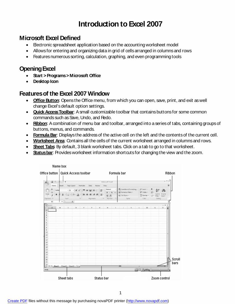
Introduction to Excel 2007

Microsoft Excel Defined Electronic spreadsheet application based on the accounting worksheet model Allows for entering and organizing data in grid of cells arranged in columns and rows Features numerous sorting, calculation, graphing, and even programming tools

Opening Excel Start > Programs > Microsoft Office Desktop Icon

Features of the Excel 2007 Window Office Button: Opens the Office menu, from which you can open, save, print, and exit as well

change Excel's default option settings. Quick Access Toolbar: A small customizable toolbar that contains buttons for some common

commands such as Save, Undo, and Redo. Ribbon: A combination of menu bar and toolbar, arranged into a series of tabs, containing groups of

buttons, menus, and commands. Formula Bar: Displays the address of the active cell on the left and the contents of the current cell. Worksheet Area: Contains all the cells of the current worksheet arranged in columns and rows. Sheet Tabs: By default, 3 blank worksheet tabs. Click on a tab to go to that worksheet. Status bar: Provides worksheet information shortcuts for changing the view and the zoom.

Create PDF files without this message by purchasing novaPDF printer (http://www.novapdf.com)

http://www.novapdf.com


2

Parts of a Worksheet Excel files are called “workbooks.” These workbooks are made up of individual worksheets, also called spreadsheets, which contain the information you enter.

Worksheets consist of individual cells formed by the intersection of columns and rows. The active cell is the cell that is currently selected. Each cell has a “cell address” of a column heading (letter) and a row heading (number), such as “A1” or “E15.”

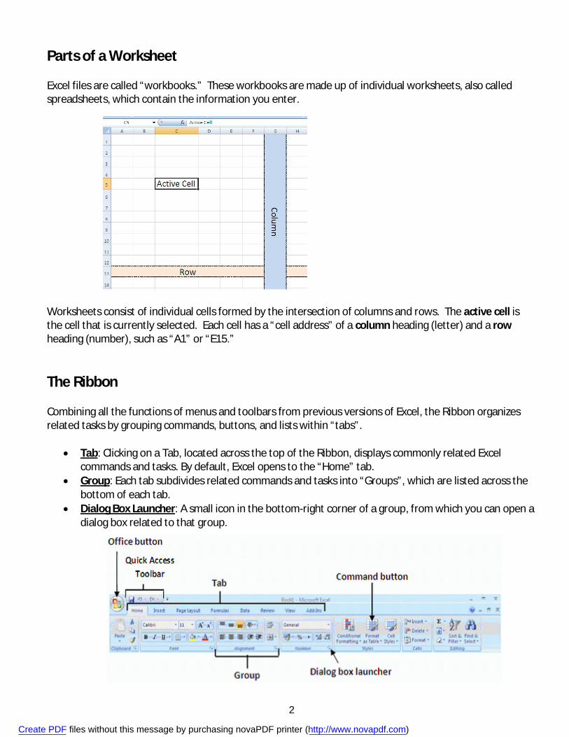
The Ribbon Combining all the functions of menus and toolbars from previous versions of Excel, the Ribbon organizes related tasks by grouping commands, buttons, and lists within “tabs”.

Tab: Clicking on a Tab, located across the top of the Ribbon, displays commonly related Excel commands and tasks. By default, Excel opens to the “Home” tab.

Group: Each tab subdivides related commands and tasks into “Groups”, which are listed across the bottom of each tab.

Dialog Box Launcher: A small icon in the bottom-right corner of a group, from which you can open a dialog box related to that group.




3

Entering Data Although you are entering information with the keyboard and mouse, editing a worksheet differs from editing a word processing document in a number of ways:

• Information is entered into each cell individually. • Although the contents of a cell may overflow into the next cell if the next cell is empty, all of the

data is contained in that first cell. • Text does not automatically word wrap. • The number of characters you can type into one cell is limited. • Numbers are not automatically treated as textual information and follow their own special rules.

o Numbers align to the right side of the cell. o When the number typed is longer than the width of the column, it will appear as a series of

pound signs (#####) or in scientific notation (4.63435E+18). o Initial zeros will be dropped (042 42). o Some number entries will be converted to pre-set formats, such as date (8-27 27-Aug).

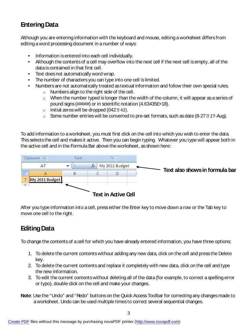
To add information to a worksheet, you must first click on the cell into which you wish to enter the data. This selects the cell and makes it active. Then you can begin typing. Whatever you type will appear both in the active cell and in the Formula Bar above the worksheet, as shown here:

After you type information into a cell, press either the Enter key to move down a row or the Tab key to move one cell to the right.

Editing Data To change the contents of a cell for which you have already entered information, you have three options:

1. To delete the current contents without adding any new data, click on the cell and press the Delete key.

2. To delete the current contents and replace it completely with new data, click on the cell and type the new information.

3. To edit the current contents without deleting all of the data (for example, to correct a spelling error or typo), double click on the cell and make your changes.

Note: Use the “Undo” and “Redo” buttons on the Quick Access Toolbar for correcting any changes made to

a worksheet. Undo can be used multiple times to correct several sequential changes.

Text in Active Cell

Text also shows in formula bar




4

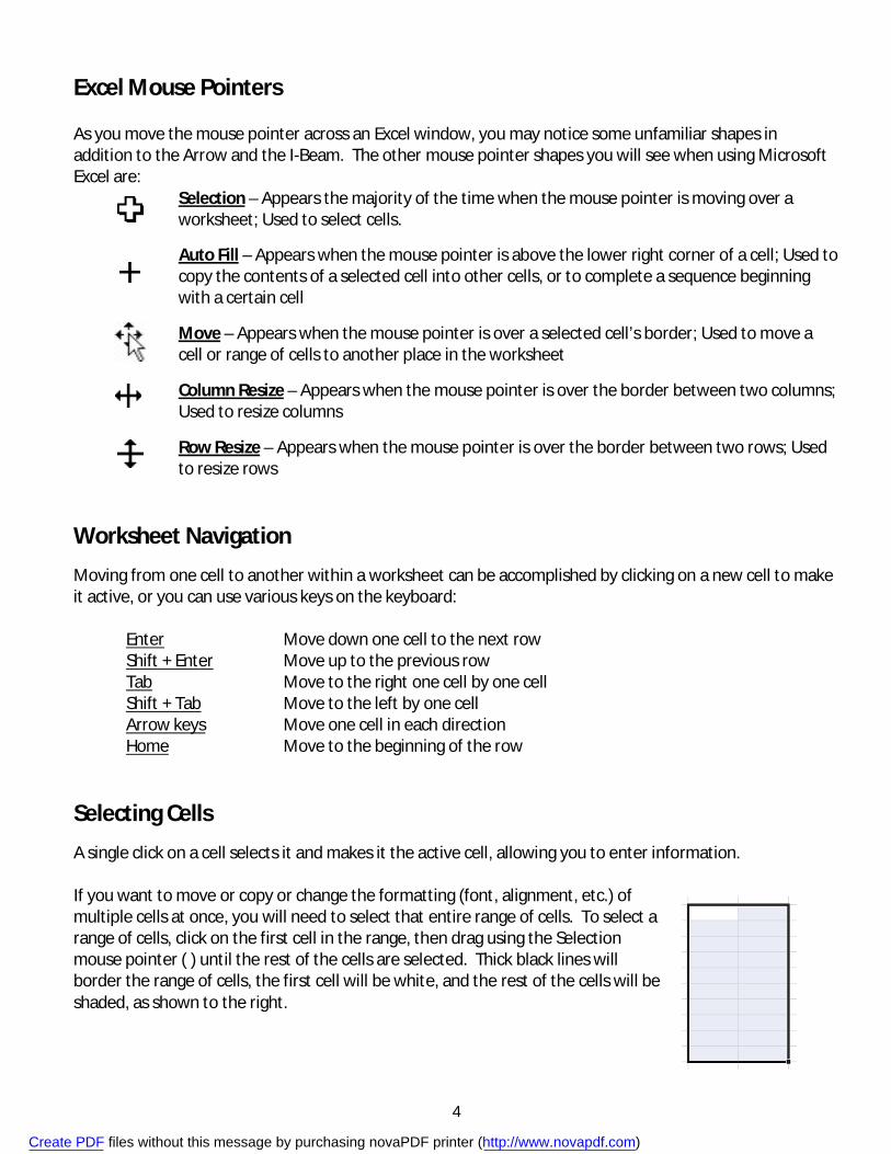
Excel Mouse Pointers As you move the mouse pointer across an Excel window, you may notice some unfamiliar shapes in addition to the Arrow and the I-Beam. The other mouse pointer shapes you will see when using Microsoft Excel are:

Selection – Appears the majority of the time when the mouse pointer is moving over a worksheet; Used to select cells.

Auto Fill – Appears when the mouse pointer is above the lower right corner of a cell; Used to copy the contents of a selected cell into other cells, or to complete a sequence beginning with a certain cell

Move – Appears when the mouse pointer is over a selected cell’s border; Used to move a cell or range of cells to another place in the worksheet

Column Resize – Appears when the mouse pointer is over the border between two columns; Used to resize columns

Row Resize – Appears when the mouse pointer is over the border between two rows; Used to resize rows

Worksheet Navigation

Moving from one cell to another within a worksheet can be accomplished by clicking on a new cell to make it active, or you can use various keys on the keyboard: Enter Move down one cell to the next row Shift + Enter Move up to the previous row Tab Move to the right one cell by one cell

Shift + Tab Move to the left by one cell Arrow keys Move one cell in each direction Home Move to the beginning of the row

Selecting Cells

A single click on a cell selects it and makes it the active cell, allowing you to enter information. If you want to move or copy or change the formatting (font, alignment, etc.) of multiple cells at once, you will need to select that entire range of cells. To select a range of cells, click on the first cell in the range, then drag using the Selection mouse pointer ( ) until the rest of the cells are selected. Thick black lines will border the range of cells, the first cell will be white, and the rest of the cells will be shaded, as shown to the right.




5

Moving Cells

A cell or range of cells can be moved from their original location to a new location within the worksheet by following these steps:

1. Select the cell or cells you wish to move, as discussed above. 2. Move the mouse directly over the thick black line bordering the cell or cells. 3. When you see the Move mouse pointer ( ) click and drag the selected cell or cells to the

new location.

Selecting Rows and Columns

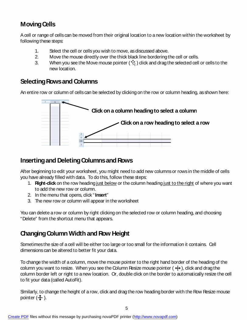
An entire row or column of cells can be selected by clicking on the row or column heading, as shown here:

Inserting and Deleting Columns and Rows

After beginning to edit your worksheet, you might need to add new columns or rows in the middle of cells you have already filled with data. To do this, follow these steps:

1. Right-click on the row heading just below or the column heading just to the right of where you want to add the new row or column.

2. In the menu that opens, click “Insert” 3. The new row or column will appear in the worksheet

You can delete a row or column by right clicking on the selected row or column heading, and choosing “Delete” from the shortcut menu that appears.

Changing Column Width and Row Height

Sometimes the size of a cell will be either too large or too small for the information it contains. Cell dimensions can be altered to better fit your data. To change the width of a column, move the mouse pointer to the right hand border of the heading of the column you want to resize. When you see the Column Resize mouse pointer ( ), click and drag the column border left or right to a new location. Or, double click on the border to automatically resize the cell to fit your data (called AutoFit). Similarly, to change the height of a row, click and drag the row heading border with the Row Resize mouse pointer ( ).

Click on a column heading to select a column

Click on a row heading to select a row




6

Using AutoSum

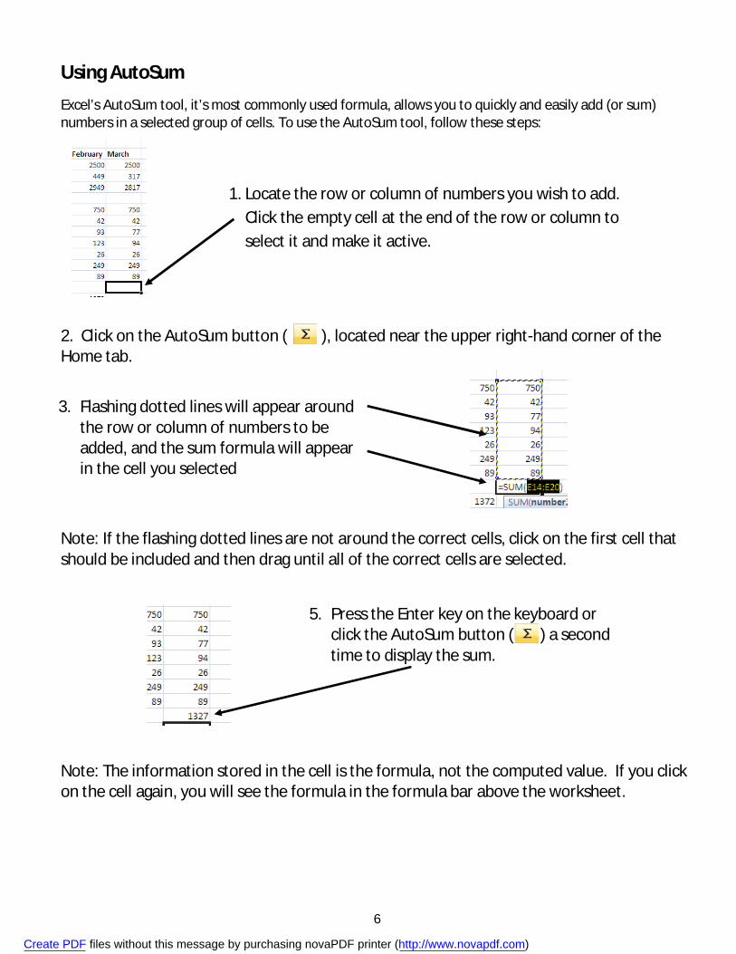
Excel’s AutoSum tool, it’s most commonly used formula, allows you to quickly and easily add (or sum) numbers in a selected group of cells. To use the AutoSum tool, follow these steps: 2. Click on the AutoSum button ( ), located near the upper right-hand corner of the Home tab. Note: If the flashing dotted lines are not around the correct cells, click on the first cell that should be included and then drag until all of the correct cells are selected. Note: The information stored in the cell is the formula, not the computed value. If you click on the cell again, you will see the formula in the formula bar above the worksheet.

1. Locate the row or column of numbers you wish to add. Click the empty cell at the end of the row or column to select it and make it active.

5. Press the Enter key on the keyboard or click the AutoSum button ( ) a second time to display the sum.

3. Flashing dotted lines will appear around the row or column of numbers to be added, and the sum formula will appear in the cell you selected




7

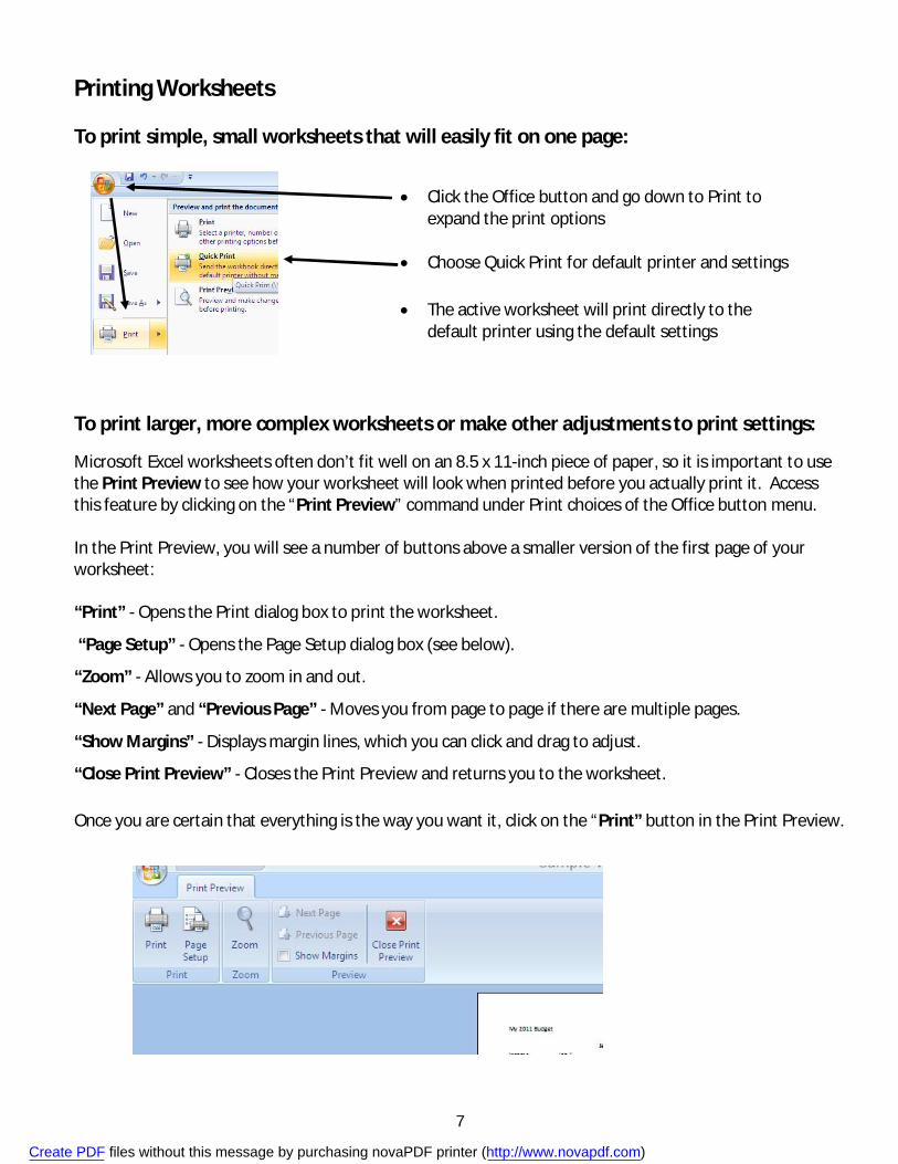
Printing Worksheets To print simple, small worksheets that will easily fit on one page: To print larger, more complex worksheets or make other adjustments to print settings:

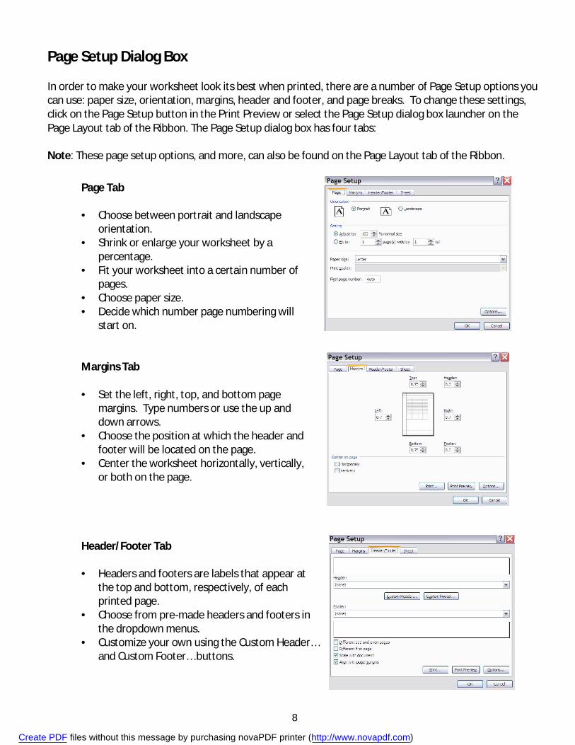
Microsoft Excel worksheets often don’t fit well on an 8.5 x 11-inch piece of paper, so it is important to use the Print Preview to see how your worksheet will look when printed before you actually print it. Access this feature by clicking on the “Print Preview” command under Print choices of the Office button menu. In the Print Preview, you will see a number of buttons above a smaller version of the first page of your worksheet: “Print” - Opens the Print dialog box to print the worksheet.

“Page Setup” - Opens the Page Setup dialog box (see below).

“Zoom” - Allows you to zoom in and out.

“Next Page” and “Previous Page” - Moves you from page to page if there are multiple pages.

“Show Margins” - Displays margin lines, which you can click and drag to adjust.

“Close Print Preview” - Closes the Print Preview and returns you to the worksheet.

Once you are certain that everything is the way you want it, click on the “Print” button in the Print Preview.

Click the Office button and go down to Print to expand the print options

Choose Quick Print for default printer and settings

The active worksheet will print directly to the default printer using the default settings




8

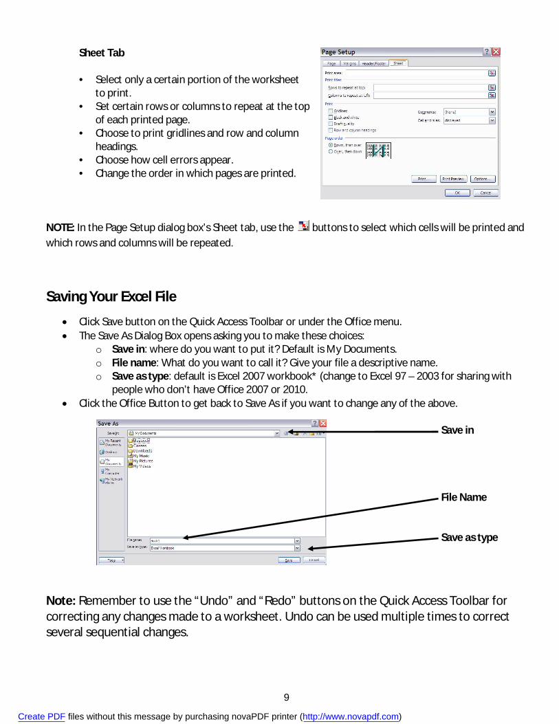
Page Setup Dialog Box In order to make your worksheet look its best when printed, there are a number of Page Setup options you can use: paper size, orientation, margins, header and footer, and page breaks. To change these settings, click on the Page Setup button in the Print Preview or select the Page Setup dialog box launcher on the Page Layout tab of the Ribbon. The Page Setup dialog box has four tabs: Note: These page setup options, and more, can also be found on the Page Layout tab of the Ribbon.

Page Tab

• Choose between portrait and landscape orientation.

• Shrink or enlarge your worksheet by a percentage.

• Fit your worksheet into a certain number of pages.

• Choose paper size. • Decide which number page numbering will

start on.

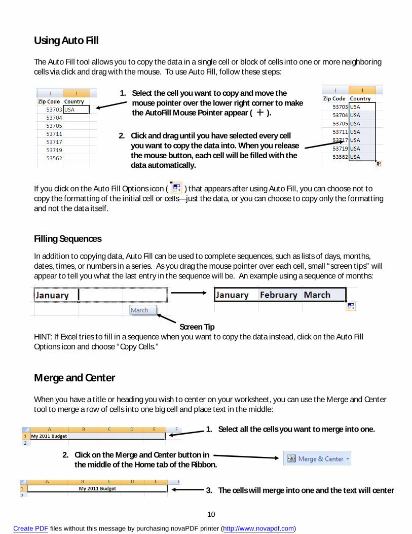
Margins Tab • Set the left, right, top, and bottom page

margins. Type numbers or use the up and down arrows.

• Choose the position at which the header and footer will be located on the page.

• Center the worksheet horizontally, vertically, or both on the page.

Header/Footer Tab • Headers and footers are labels that appear at

the top and bottom, respectively, of each printed page.

• Choose from pre-made headers and footers in the dropdown menus.

• Customize your own using the Custom Header… and Custom Footer… buttons.




9

Sheet Tab • Select only a certain portion of the worksheet

to print. • Set certain rows or columns to repeat at the top

of each printed page. • Choose to print gridlines and row and column

headings. • Choose how cell errors appear. • Change the order in which pages are printed.

NOTE: In the Page Setup dialog box’s Sheet tab, use the buttons to select which cells will be printed and which rows and columns will be repeated.

Saving Your Excel File

Click Save button on the Quick Access Toolbar or under the Office menu. The Save As Dialog Box opens asking you to make these choices:

o Save in: where do you want to put it? Default is My Documents. o File name: What do you want to call it? Give your file a descriptive name. o Save as type: default is Excel 2007 workbook* (change to Excel 97 – 2003 for sharing with

people who don’t have Office 2007 or 2010. Click the Office Button to get back to Save As if you want to change any of the above.

Save in

File Name

Save as type

Note: Remember to use the “Undo” and “Redo” buttons on the Quick Access Toolbar for correcting any changes made to a worksheet. Undo can be used multiple times to correct several sequential changes.




10

Using Auto Fill The Auto Fill tool allows you to copy the data in a single cell or block of cells into one or more neighboring cells via click and drag with the mouse. To use Auto Fill, follow these steps:

If you click on the Auto Fill Options icon ( ) that appears after using Auto Fill, you can choose not to copy the formatting of the initial cell or cells—just the data, or you can choose to copy only the formatting and not the data itself. Filling Sequences

In addition to copying data, Auto Fill can be used to complete sequences, such as lists of days, months, dates, times, or numbers in a series. As you drag the mouse pointer over each cell, small “screen tips” will appear to tell you what the last entry in the sequence will be. An example using a sequence of months:

Screen Tip HINT: If Excel tries to fill in a sequence when you want to copy the data instead, click on the Auto Fill Options icon and choose “Copy Cells.”

Merge and Center When you have a title or heading you wish to center on your worksheet, you can use the Merge and Center tool to merge a row of cells into one big cell and place text in the middle:

1. Select the cell you want to copy and move the mouse pointer over the lower right corner to make the AutoFill Mouse Pointer appear ( ).

2. Click and drag until you have selected every cell you want to copy the data into. When you release the mouse button, each cell will be filled with the data automatically.

1. Select all the cells you want to merge into one.

2. Click on the Merge and Center button in the middle of the Home tab of the Ribbon.

3. The cells will merge into one and the text will center




11

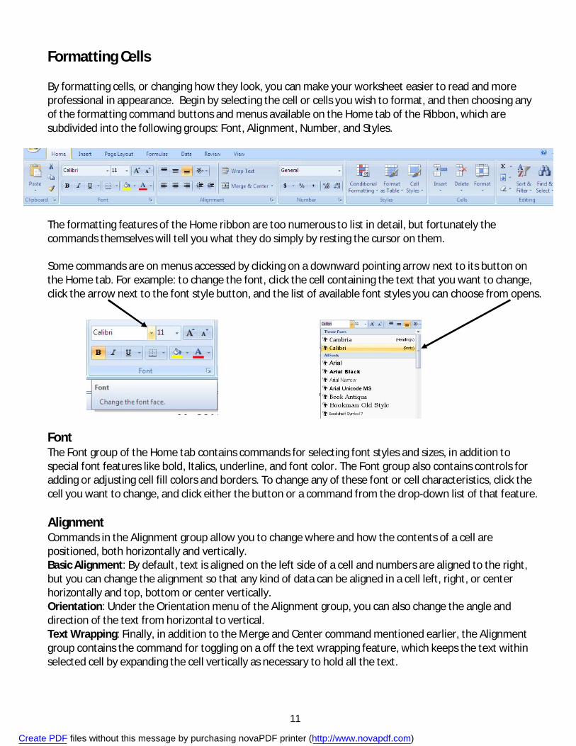
Formatting Cells By formatting cells, or changing how they look, you can make your worksheet easier to read and more professional in appearance. Begin by selecting the cell or cells you wish to format, and then choosing any of the formatting command buttons and menus available on the Home tab of the Ribbon, which are subdivided into the following groups: Font, Alignment, Number, and Styles. The formatting features of the Home ribbon are too numerous to list in detail, but fortunately the commands themselves will tell you what they do simply by resting the cursor on them. Some commands are on menus accessed by clicking on a downward pointing arrow next to its button on the Home tab. For example: to change the font, click the cell containing the text that you want to change, click the arrow next to the font style button, and the list of available font styles you can choose from opens.

Font The Font group of the Home tab contains commands for selecting font styles and sizes, in addition to special font features like bold, Italics, underline, and font color. The Font group also contains controls for adding or adjusting cell fill colors and borders. To change any of these font or cell characteristics, click the cell you want to change, and click either the button or a command from the drop-down list of that feature. Alignment Commands in the Alignment group allow you to change where and how the contents of a cell are positioned, both horizontally and vertically. Basic Alignment: By default, text is aligned on the left side of a cell and numbers are aligned to the right, but you can change the alignment so that any kind of data can be aligned in a cell left, right, or center horizontally and top, bottom or center vertically. Orientation: Under the Orientation menu of the Alignment group, you can also change the angle and direction of the text from horizontal to vertical. Text Wrapping: Finally, in addition to the Merge and Center command mentioned earlier, the Alignment group contains the command for toggling on a off the text wrapping feature, which keeps the text within selected cell by expanding the cell vertically as necessary to hold all the text.




12

Number The Number group allows you to choose a number format, such as Currency, Date, Time, Percentage, Zip Code, and Phone Number, etc. You may also choose the Text format to have cell contents treated as text instead of numbers.

There are three ways of accessing these Number format choices:

Format Painter The Format Painter icon ( ) on the Home tab allows you to easily apply the formatting of one cell to other cells in the worksheet. Click on the cell with the desired formatting, then click on the Format Painter icon. A little paintbrush will appear next to the mouse pointer. Then click on the cell or range of cells you wish to apply the formatting to. Note: Many other predefined formatting tools can be found in the Themes group of the Page Layout ribbon tab, which makes changes to the whole document, and in the Styles group of the Home ribbon tab, which provides specialized formatting for selected cells.

Freezing Panes

Freeze Panes is a handy tool for keeping a portion of the sheet visible (like a heading row) while the rest of the sheet scrolls. There are three choices under the Freeze Panes command of the View Ribbon tab: Freeze Panes (freezing adjacent to selected cells), Freeze top Row, or Freeze First Column. For example, to keep a heading row fixed so that it remains visible when scrolling down (if it isn’t the top row), follow these steps:

1. Click the row heading just below the row you want to freeze so that the row is selected.

2. Click on the View Ribbon tab, click the Freeze Panes button, and then click on the Freeze Panes command at the top of the list that opens.

3. The rows above the one selected will now stay visible even when you scroll down the sheet.

1. Clicking on the drop-down list at the top of the group contains Styles commands for General, Number, Currency, Accounting, Short Date, Long Date, Time Percentage, and Fractions.

2. Buttons for the number formatting options Currency Style, Percent Style, Comma Style, Increase Decimal, and Decrease Decimal are located directly on the group.

3. To see the full set of Number formatting choices, click the little dialog box launcher in the lower right corner of the group.




13

Formulas Programs like Microsoft Excel were originally created to store and manipulate numerical data. You can use formulas to tell the computer that you want to perform a mathematical calculation. Formulas always begin with an equal sign (=), and they are made up of cell addresses, which stand for the values in those cells; operators; and numbers. Operators include:

+ Addition * Multiplication - Subtraction / Division % Percentage ^ Exponentiation

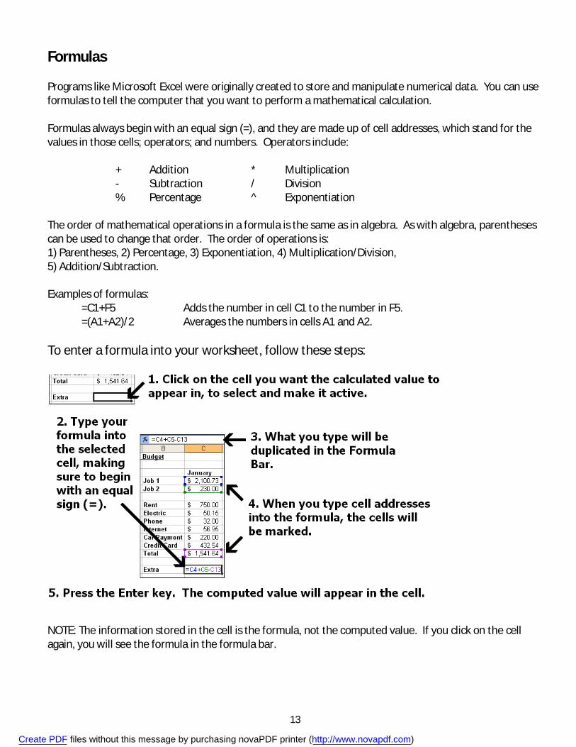
The order of mathematical operations in a formula is the same as in algebra. As with algebra, parentheses can be used to change that order. The order of operations is: 1) Parentheses, 2) Percentage, 3) Exponentiation, 4) Multiplication/Division, 5) Addition/Subtraction. Examples of formulas: =C1+F5 Adds the number in cell C1 to the number in F5. =(A1+A2)/2 Averages the numbers in cells A1 and A2. To enter a formula into your worksheet, follow these steps:

NOTE: The information stored in the cell is the formula, not the computed value. If you click on the cell again, you will see the formula in the formula bar.




14

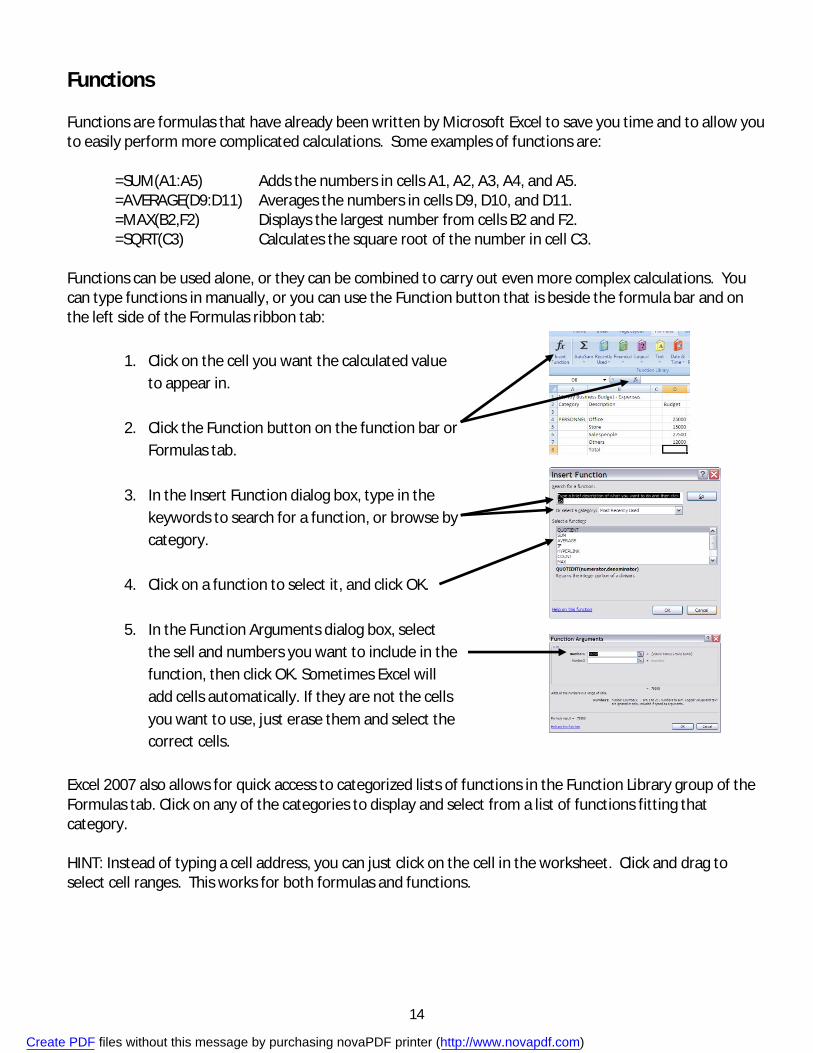
Functions Functions are formulas that have already been written by Microsoft Excel to save you time and to allow you to easily perform more complicated calculations. Some examples of functions are: =SUM(A1:A5) Adds the numbers in cells A1, A2, A3, A4, and A5. =AVERAGE(D9:D11) Averages the numbers in cells D9, D10, and D11. =MAX(B2,F2) Displays the largest number from cells B2 and F2. =SQRT(C3) Calculates the square root of the number in cell C3. Functions can be used alone, or they can be combined to carry out even more complex calculations. You can type functions in manually, or you can use the Function button that is beside the formula bar and on the left side of the Formulas ribbon tab: Excel 2007 also allows for quick access to categorized lists of functions in the Function Library group of the Formulas tab. Click on any of the categories to display and select from a list of functions fitting that category. HINT: Instead of typing a cell address, you can just click on the cell in the worksheet. Click and drag to select cell ranges. This works for both formulas and functions.

1. Click on the cell you want the calculated value to appear in.

2. Click the Function button on the function bar or Formulas tab.

3. In the Insert Function dialog box, type in the keywords to search for a function, or browse by category.

4. Click on a function to select it, and click OK.

5. In the Function Arguments dialog box, select the sell and numbers you want to include in the function, then click OK. Sometimes Excel will add cells automatically. If they are not the cells you want to use, just erase them and select the correct cells.




15

Fixing Function Errors Microsoft Excel will automatically check for errors in the formulas and functions you enter, and it will usually offer suggestions for correction and other help as well. The two main tools used for error checking and correction are Formula AutoCorrect and background error checking. Formula AutoCorrect catches operator errors, including:

• Unmatched parentheses: “=250/(C4+C5” instead of “=250/(C4+C5)” • Reversed cell references: “=15A-15B” instead of “=A15-B15” • Double operators: “==A2*1.25” instead of “=A2*1.25”

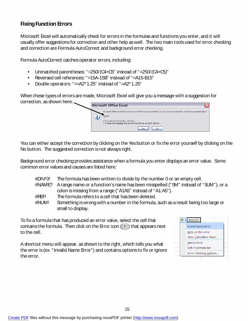
When these types of errors are made, Microsoft Excel will give you a message with a suggestion for correction, as shown here: You can either accept the correction by clicking on the Yes button or fix the error yourself by clicking on the No button. The suggested correction is not always right. Background error checking provides assistance when a formula you enter displays an error value. Some common error values and causes are listed here:

#DIV/0! The formula has been written to divide by the number 0 or an empty cell. #NAME? A range name or a function’s name has been misspelled (“SM” instead of “SUM”), or a

colon is missing from a range (“A1A5” instead of “A1:A5”). #REF! The formula refers to a cell that has been deleted. #NUM! Something is wrong with a number in the formula, such as a result being too large or

small to display. To fix a formula that has produced an error value, select the cell that contains the formula. Then click on the Error icon ( ) that appears next to the cell. A shortcut menu will appear, as shown to the right, which tells you what the error is (ex. “Invalid Name Error”) and contains options to fix or ignore the error.




16

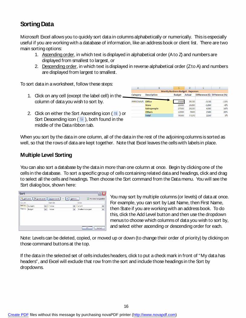
Sorting Data Microsoft Excel allows you to quickly sort data in columns alphabetically or numerically. This is especially useful if you are working with a database of information, like an address book or client list. There are two main sorting options:

1. Ascending order, in which text is displayed in alphabetical order (A to Z) and numbers are displayed from smallest to largest, or

2. Descending order, in which text is displayed in reverse alphabetical order (Z to A) and numbers are displayed from largest to smallest.

To sort data in a worksheet, follow these steps:

1. Click on any cell (except the label cell) in the column of data you wish to sort by.

2. Click on either the Sort Ascending icon ( ) or Sort Descending icon ( ), both found in the middle of the Data ribbon tab.

When you sort by the data in one column, all of the data in the rest of the adjoining columns is sorted as well, so that the rows of data are kept together. Note that Excel leaves the cells with labels in place. Multiple Level Sorting You can also sort a database by the data in more than one column at once. Begin by clicking one of the cells in the database. To sort a specific group of cells containing related data and headings, click and drag to select all the cells and headings. Then choose the Sort command from the Data menu. You will see the Sort dialog box, shown here:

You may sort by multiple columns (or levels) of data at once. For example, you can sort by Last Name, then First Name, then State if you are working with an address book. To do this, click the Add Level button and then use the dropdown menus to choose which columns of data you wish to sort by, and select either ascending or descending order for each.

Note: Levels can be deleted, copied, or moved up or down (to change their order of priority) by clicking on those command buttons at the top. If the data in the selected set of cells includes headers, click to put a check mark in front of “My data has headers”, and Excel will exclude that row from the sort and include those headings in the Sort by dropdowns.




17

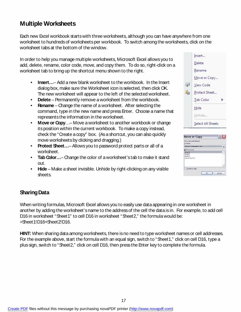
Multiple Worksheets Each new Excel workbook starts with three worksheets, although you can have anywhere from one worksheet to hundreds of worksheets per workbook. To switch among the worksheets, click on the worksheet tabs at the bottom of the window. In order to help you manage multiple worksheets, Microsoft Excel allows you to add, delete, rename, color code, move, and copy them. To do so, right-click on a worksheet tab to bring up the shortcut menu shown to the right.

• Insert… – Add a new blank worksheet to the workbook. In the Insert dialog box, make sure the Worksheet icon is selected, then click OK. The new worksheet will appear to the left of the selected worksheet.

• Delete – Permanently remove a worksheet from the workbook. • Rename – Change the name of a worksheet. After selecting the

command, type in the new name and press Enter. Choose a name that represents the information in the worksheet.

• Move or Copy… – Move a worksheet to another workbook or change its position within the current workbook. To make a copy instead, check the “Create a copy” box. (As a shortcut, you can also quickly move worksheets by clicking and dragging.)

• Protect Sheet… – Allows you to password protect parts or all of a worksheet.

• Tab Color… – Change the color of a worksheet’s tab to make it stand out.

• Hide – Make a sheet invisible. Unhide by right-clicking on any visible sheets.

Sharing Data When writing formulas, Microsoft Excel allows you to easily use data appearing in one worksheet in another by adding the worksheet’s name to the address of the cell the data is in. For example, to add cell D16 in worksheet “Sheet1” to cell D16 in worksheet “Sheet2,” the formula would be: =Sheet1!D16+Sheet2!D16. HINT: When sharing data among worksheets, there is no need to type worksheet names or cell addresses. For the example above, start the formula with an equal sign, switch to “Sheet1,” click on cell D16, type a plus sign, switch to “Sheet2,” click on cell D16, then press the Enter key to complete the formula.




18

Charts and Graphs Microsoft Excel lets you turn your raw data into a variety of charts and graphs. Using this feature, you can visually summarize numerical information and display any trends or patterns that are present. Charts and graphs can help make your data more meaningful and easier to understand. When you create a chart or graph, you will have a number of types and styles to choose from. Make sure to choose the chart type that best displays your data. These are the most commonly used types of charts:

Column – Column charts are made up of vertical bars representing multiple sets of data. They are most often used to show how amounts have changed over time. Bar – Bar charts are made up of horizontal bars representing multiple sets of data. They are most often used to compare various amounts at a fixed point in time. Line – Line charts are made up of lines representing multiple sets of data. They are most often used to show changes over time and are good for emphasizing trends. Pie – Pie charts are made up of “slices” representing a single set of data. They are most often used to show how parts relate to the whole.

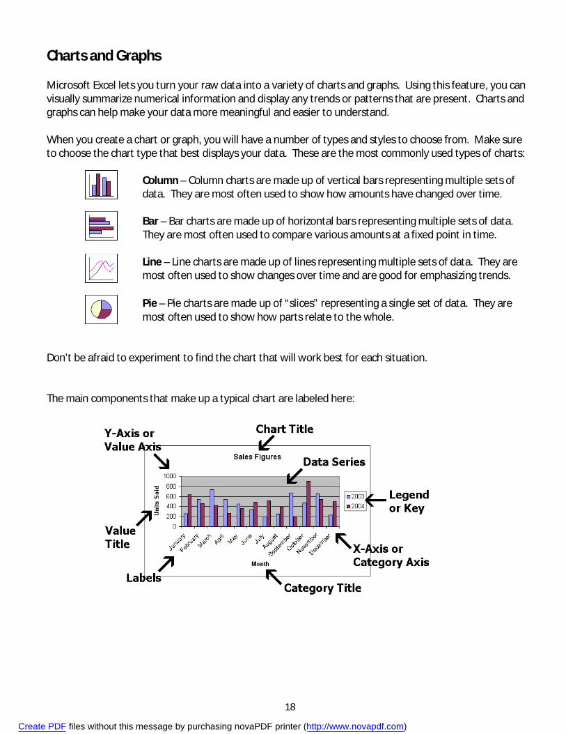
Don’t be afraid to experiment to find the chart that will work best for each situation. The main components that make up a typical chart are labeled here:




19

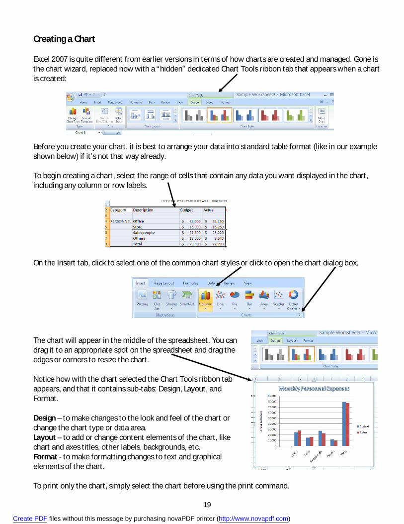
Creating a Chart Excel 2007 is quite different from earlier versions in terms of how charts are created and managed. Gone is the chart wizard, replaced now with a “hidden” dedicated Chart Tools ribbon tab that appears when a chart is created: Before you create your chart, it is best to arrange your data into standard table format (like in our example shown below) if it’s not that way already. To begin creating a chart, select the range of cells that contain any data you want displayed in the chart, including any column or row labels. On the Insert tab, click to select one of the common chart styles or click to open the chart dialog box. The chart will appear in the middle of the spreadsheet. You can drag it to an appropriate spot on the spreadsheet and drag the edges or corners to resize the chart. Notice how with the chart selected the Chart Tools ribbon tab appears, and that it contains sub-tabs: Design, Layout, and Format. Design – to make changes to the look and feel of the chart or change the chart type or data area. Layout – to add or change content elements of the chart, like chart and axes titles, other labels, backgrounds, etc. Format - to make formatting changes to text and graphical elements of the chart. To print only the chart, simply select the chart before using the print command.


