Embed Size (px)
Citation preview

Introduction to
Compressed
Sensing With Coding Theoretic Perspective This book is a course note developed for a graduate level course in Spring 2011, at GIST, Korea. The course aimed at introducing the topic of Compressed Sensing (CS). CS is considered as a new signal acquisition paradigm with which sample taking could be faster than what can be expected of the canonical approach. Namely, the number of signal samples sufficient to reproduce a given signal could be much smaller than the number of samples deemed sufficient under the Shannon Nyquist sampling theory. The CS theory is expected to influence many application areas with interruptive changes to their current practices in the years to come, including tomography, radars, communications, image and signal processing, and wireless sensor networks. In addition, we make note of the fact that the tenet of CS theory is equivalent to the parity-checking and syndrome decoding in the Channel Coding theory. On the one hand, this means that, wealth of information is available to solve the parity-check equation from Channel Coding theory which can be leveraged to understand the CS problem better; on the other hand, the new information being generated in the CS community can be utilized to provide new perspectives in advancing the Channel Coding theory.
Heung-No Lee
8/29/2011

1
1 0: Acknowledgement
Table of Contents
Acknowledgement ............................................................................................................. 4 Chapter I. Course Information ............................................................................................... 5
1. General Information ..................................................................................................... 5 2. Course Syllabus ........................................................................................................... 6 3. How to Cite this Note .................................................................................................. 8 4. Course Scope and Materials ........................................................................................ 8 5. The RICE University Repository ............................................................................... 11 6. Applications ............................................................................................................... 12
A. Single Pixel Cameras ................................................................................... 12 B. Terahertz pulsed spectroscopic imaging ...................................................... 12 C. Other areas of applications .......................................................................... 15 D. Summary of Applications ............................................................................ 15
7. References .................................................................................................................. 15 Chapter II. Compressed Sensing ........................................................................................... 16
1. Compressed Sensing, Compressive Sensing, Compressive Sampling ...................... 16 2. Pioneers of Compressed Sensing ............................................................................... 16 3. Sampling Theorem and Dimensionality Reduction by Shannon ............................... 17 4. Compressed Sensing in a Nutshell ............................................................................ 20 5. Compressed Sensing, explained with a little more care ............................................ 22
A. Restricted Isometry Property ....................................................................... 23 B. Incoherence Condition ................................................................................. 24 C. Checking RIP is NP-hard. ............................................................................ 24 D. L0, L1, L2 norms and the null space ........................................................... 26
6. Summary .................................................................................................................... 29 7. The Spark and The Singleton Bound ......................................................................... 29 8. Matrix Design with Givens Rotations ....................................................................... 30 9. Super Resolution Applications (Nano array filters and Nano lenses) ....................... 32 10. HW set #1 ........................................................................................................... 36 11. References for Chapter 2 .................................................................................... 38
Chapter III. Mathematics of Compressive Sensing ......................................................... 39 1. Uncertainty Principle and the L1 Uniqueness Proof ................................................. 41
A. Representation via a Combined Dictionary ................................................. 42 B. The Uncertainty Principle ............................................................................ 44 C. The Theorem on the Uniqueness of the L0 Optimization ........................... 45 D. Uniqueness of the L1 Optimization ............................................................. 46
2. The Uniform Uncertainty Principle ........................................................................... 52 A. Sufficient and Necessary Conditions for the Unique L0 Solution .............. 53 B. Condition for the Unique L1 Solution ......................................................... 56
3. Uniqueness Proofs with Mutual Coherence μ ........................................................ 64
A. Comparison of , ,2K K K Kθ θ+ and K μ ....................................................... 64
B. Connections to Other Results ...................................................................... 66 4. Ensembles of Random Sensing Matrices .................................................................. 70
A. The log(N) factor for random ensembles ..................................................... 70 B. The log(N) factor, is it really needed for a random sensing matrix? ........... 70 C. The log(N) factor, deriven for binary K-sparse signals ............................... 72
5. Stable Recovery Property .......................................................................................... 74

2 Chapter I: Course Information
6. The Chapter Problems ............................................................................................... 75 Chapter IV. Information Theoretic Considertation ......................................................... 79
1. K-sparse signal model ................................................................................................ 79 2. The Entropy of K-sparse signals ................................................................................ 81 3. Mutual Information .................................................................................................... 83 4. Lower Bound on Probability of Sensing Error via Fano’s Inequality ....................... 84
Chapter V. Sparse Recovery Algorithms .............................................................................. 86 1. Linear Programming .................................................................................................. 86 2. Solving Linear Program via Lagrange Dual Interior Point Method .......................... 88 3. Solving Second Order Cone Programs with Log-Barrier Method ............................ 93
A. A log barrier function .................................................................................. 94 B. The interior log barrier method for solving SOCPs .................................... 95
4. Homotopy Algorithms ............................................................................................... 99 A. Motivation ................................................................................................... 99 B. The Homotopy Problem .............................................................................. 99 C. Two constraints from the subdifferential ................................................... 102 D. The Homotopy Algorithm ......................................................................... 103 E. Proof of the Theorem ................................................................................. 107
5. Bayesian Compressive Sensing on the Graph Model .............................................. 110 A. Iterative Compressive Sensing Algorithm ................................................. 111 B. The Distribution of the Signal Value ......................................................... 112 C. The Distribution of the Signal Value in the Presence of Noise ................. 115 D. Distribution of the Binary State Value ....................................................... 115 E. Useful Mathematical Identities for Log-Sum-Products ............................. 120 F. The Message Passing Algorithm ...................................................................... 121 G. Donoho’s message passing algorithm for compressed sensing ................. 121
6. The Expander Graph Approach ............................................................................... 122 7. Section References ................................................................................................... 123 8. Chapter Problems ..................................................................................................... 124
Chapter VI. Recent Research Results ............................................................................ 126 1. Deterministic Matrix Design ................................................................................... 126 2. Coding Theoretic Approach ..................................................................................... 126
A. Compressed Sensing via Syndrome Decoding .......................................... 126 B. The Sparks of Sensing Matrices over GF(q) ............................................. 129 C. Signal Detection Algorithms ..................................................................... 130 D. Simulation Results ..................................................................................... 132 E. Section Summary ....................................................................................... 133 F. Section References ........................................................................................... 133
3. Representation via Correlation vs. via Sparseness .................................................. 134 Chapter VII. Review of Mathematical Results ............................................................... 135
1. Directional Derivatives, Subgradients, and Subdifferentials ................................... 135 2. Duality and Convex Optimization ........................................................................... 139 3. Some Useful Linear Algebra Results ....................................................................... 149
A. Some Facts on the Matrix Norm ............................................................... 149 B. Other useful matrix norm properties ......................................................... 149
Chapter VIII. References ................................................................................................. 151

3
3 0: Acknowledgement
Table of Figures
Figure 1: Fig. 2 of Shannon [1] .................................................................................................................. 19 Figure 2 : A chart from [15]. ...................................................................................................................... 41 Figure 3 : A chart from [15]. ...................................................................................................................... 42 Figure 4: An example of linear objective function [ ]min 1 1 s.t. 1 0T
xx x x− − ≤ . Note that the
optimal point is achieved at the perimeter of the feasible set. ............................................................ 89 Figure 5: The Concept of Placing Barriers At the Boundary of the Feasible Set ....................................... 94 Figure 6: A log-barrier function ................................................................................................................. 95 Figure 7: Variation of the penalized objective function as lambda is changing from 4 to 0. .................... 100 Figure 8: Relation map of algorithms. From Donoho and Tsaig [18]. ..................................................... 102 Figure 9: The Graph ................................................................................................................................. 112 Figure 10 : Gilbert-Varshamov Compressed Sensing Bounds for Sensing Matrices over GF(q) and The
Singleton Bound ................................................................................................................................ 129 Figure 11 : Simulation results of a C(N=1200, ds = 3, dc = 6) code with different field sizes. ................. 132 Figure 12: Hyperplane .............................................................................................................................. 135 Figure 13: Geometrical illustration of a subgradient of a convex function f. Note that the space is n + 1
dimensional. ...................................................................................................................................... 136 Figure 14: Illustration of subgradients ..................................................................................................... 137 Figure 15: Geometrical illustration of a subgradient of a convex function f. Note that the space is n + 1
dimensional. ...................................................................................................................................... 138 Figure 16: The trajectory of L(x, λ) with λ is varied from 0.4 to 4. .......................................................... 143 Figure 17: Illustration of the duality gap .................................................................................................. 143

4 Chapter I: Course Information
Acknowledgement This work was supported by the National Research Foundation of Korea (NRF) grant funded by the Korean government (MEST) (Do-Yak Research Program, No. 2010-0017944) This book of lecture notes has been developed under the generous support of National Research Foundation of Korea. Contributors: There are numerous contributors to this book. They are the students and researchers in the INFONET lab. Students who have taken the course contributed providing feedbacks to the lecture materials, completing homework problems, and generating the best effort homework solution manuals. Some of the researchers in the lab have presented a summary of relevant papers at the INFONET journal club.

5
5 1: General Information
Chapter I. COURSE INFORMATION 1. General Information Instructor: Heung-No Lee, Ph.D., Associate Professor, GIST, Korea. Address: Gwangju Institute of Science and Technology, 261 Cheomdan Gwagiro, Gwangju, Republic of Korea. Phone: (82) 62-715-2237, 3140. E-mail: [email protected]. Home page: http://infonet.gist.ac.kr/ Open Source Policy
• The research trend is to moving towards “reproducible researches.”
• The homeworks and term projects submitted shall be reproducible as well.

6 Chapter I: Course Information
2. Course Syllabus I will use the following course schedule which will be posted at the course website at http://infonet.gist.ac.kr/. Course Schedule Weekly Schedule Remarks 1st Week GIST Entrance Ceremony 2nd Week 3/7, 3/9
Introduction to Compressed Sensing, Shannon Nyquist Sampling Theorem Richard Baraniuk, Compressive sensing. (IEEE Signal
Processing Magazine, 24(4), pp. 118-121, July 2007)
Justin Romberg, Imaging via compressive sampling.
(IEEE Signal Processing Magazine, 25(2), pp. 14 - 20,
March 2008)
3rd Week 3/14, 3/16
Compressive Sensing Theory: L0, L1, L2 solutions HW#1 Out
4th Week 3/21, 23
Compressive Sensing Theory: L0 and L1 equivalence,
5th Week
3/28, 30 Compressive Sensing Theory: Generalized Uncertainty Principle, Sparse Representation, conditions for the unique L0 solution, and the unique L1 solution
1. D. Donoho and X. Huo, “Uncertainty Principles and
Ideal Atomic Decomposition,” IEEE Trans. on Info.
Theory, vol.47, no.7, Nov. 2001.
2. M. Elad and A. Bruckstein, “A generalized
uncertainty principle and sparse representation in
pairs of bases,” IEEE Trans. Info. Theory, vol. 48, no.
9, Sept. 2002.
HW#2 Out
6th Week 4/4, 6
Compressive Sensing Theory: conditions for the L0 solution, and the unique L1 solution, the Candes-Tao’s approach
1. Emmanuel Candès and Terence Tao, Decoding by
linear programming. (IEEE Trans. on Information
Theory, 51(12), pp. 4203 - 4215, December 2005)
2. Emmanuel Candès, Justin Romberg, and Terence
Tao, Robust uncertainty principles: Exact signal
reconstruction from highly incomplete frequency
information. (IEEE Trans. on Information Theory,
52(2) pp. 489 - 509, February 2006)

7
7 2: Course Syllabus
3. Emmanuel Candès and Terence Tao, “Near optimal
signal recovery from random projections: Universal
encoding strategies” (IEEE Trans. on Information
Theory, 52(12), pp. 5406 - 5425, December 2006)
7th Week
4/11, 13 Sensing matrices and oversampling factors HW#3 Out
8th Week
4/18, 20 Stable Recovery
9th Week
4/25, 27 Midterm Exam
10th
Week
5/2, 4
Recovery Algorithm I: Homotopy, LASSO, LARs, OMP HW#4 Out
11th
Week
5/9, 11
Recovery Algorithm II: L1 minimization, Interior Point Methods, Log Barrier Methods
12th
Week
5/16, 18
L1-Magic packages HW#5 Out
13th
Week
5/23, 25
Bayesian Recovery Algorithm
14th
Week
5/30, 6/1
Message Passing Algorithms: Support Set Recovery
HW#6 Out
15th
Week
6/6, 8
Memorial Day, Overview of the course
16th
Week
Final Term Paper Due

8 Chapter I: Course Information
3. How to Cite this Note Please use the following line when you quote the materials in this book. Heung-No Lee, Introduction to Compressed Sensing (Lecture notes), Spring
Semester, 2011.
4. Course Scope and Materials The following materials will be discussed in class: Please note that all of these papers are available just by clicking the link or at the RICE’s Compressive Sensing web-site: http://dsp.rice.edu/cs/. Introduction to Compressive Sensing
4. Richard Baraniuk, Compressive sensing. (IEEE Signal Processing Magazine, 24(4),
pp. 118-121, July 2007)
5. Justin Romberg, Imaging via compressive sampling. (IEEE Signal Processing
Magazine, 25(2), pp. 14 - 20, March 2008)
6. David Donoho and Yaakov Tsaig, Extensions of compressed sensing. (Signal
Processing, 86(3), pp. 533-548, March 2006)
Compressive Sensing Theory 7. Emmanuel Candès, Justin Romberg, and Terence Tao, Robust uncertainty principles:
Exact signal reconstruction from highly incomplete frequency information. (IEEE
Trans. on Information Theory, 52(2) pp. 489 - 509, February 2006)
8. Emmanuel Candès and Terence Tao, “Near optimal signal recovery from random
projections: Universal encoding strategies” (IEEE Trans. on Info. Theory, 52(12), pp.
5406 - 5425, December 2006)
9. David Donoho, Compressed sensing. (IEEE Trans. on Info. Theory, 52(4), pp. 1289 -
1306, April 2006)
10. D. Donoho and X. Huo, “Uncertainty Principles and Ideal Atomic Decomposition,”
IEEE Trans. on Info. Theory, vol.47, no.7, Nov. 2001.
11. M. Elad and A. Bruckstein, “A generalized uncertainty principle and sparse
representation in pairs of bases,” IEEE Trans. Info. Theory, vol. 48, no. 9, Sept. 2002.
12. Scott S. Chen, D. Donoho, and M. Saunders, “Atomic Decomposition by Basis
Pursuit,” SIAM J. Sci. Comput. 20, pp. 33-61, vol.20, no.1, 1999.

9
9 4: Course Scope and Materials
Recovery Algorithms 13. David Donoho and Yaakov Tsaig, Fast solution of L1-norm minimization problems
when the solution may be sparse. (Stanford University Department of Statistics
Technical Report 2006-18, 2006)
14. Jacob Mattingley and Stephen Boyd, “Real-time convex optimization in Signal
Processing,” IEEE Signal Processing Magazine, pp.50 – 61, May, 2010.
(Source @ http://www.stanford.edu/~boyd/papers/rt_cvx_sig_proc.html ).
Disciplined CVX Programming
The Robust Kalman Filtering example
15. Michael Zibulevsky and Michael Elad, “L1-L2 Optimization in Signal and Image
Processing,” IEEE Signal Processing Magazine, pp. 76-88, May, 2010.
16. D. Donoho, A. Maleki, and A. Montanari, “Message passing algorithms for
compressed sensing,” PNAS, Nov. 10, 2009.
Connections to Shannon Theory/Coding Theory 17. The Shannon’s 1948 paper
18. The Rate Distortion Theory (Information Theory, Cover and Thomas)
19. Emmanuel Candès and Terence Tao, Decoding by linear programming. (IEEE Trans.
on Information Theory, 51(12), pp. 4203 - 4215, December 2005)
20. Emmanuel Candès and Terence Tao, Error correction via linear programming.
(Preprint, 2005)
21. Goyal, V.K., Fletcher, A.K., and Rangan, S.; , "Compressive Sampling and Lossy
Compression," Signal Processing Magazine, IEEE , vol.25, no.2, pp.48-56, March
2008.
doi: 10.1109/MSP.2007.915001
URL: http://www.ieeexplore.ieee.org/stamp/stamp.jsp?tp=&arnumber=4472243&isn
umber=4472102.
22. Pier Luigi Dragotti, Martin Vetterli, and Thierry Blu, Sampling moments and
reconstructing signals of finite rate of innovation: Shannon meets Strang-Fix. (IEEE
Trans. on Signal Processing, 55(7), pp. 1741-1757, May 2007)
23. Gongguo Tang, Arye Nehorai, Performance analysis for sparse support recovery.
(Preprint, Nov 2009)
24. D. Baron, M.F. Duarte, and M.B. Wakin, “Distributed Compressive Sensing,” Dror
Baron, Marco F. Duarte, Michael B. Wakin, Shriram Sarvotham, and Richard G.

10 Chapter I: Course Information
Baraniuk, Distributed compressive sensing. (Preprint, 2005) [See also related
technical report and conference publications: Allerton 2005, Asilomar 2005, NIPS
2005, IPSN 2006]
25. Robert Calderbank and Sina Jafarpour, Reed Muller Sensing Matrices and the Lasso
(Preprint, April 2010)
26. Maxim Raginsky, Sina Jafarpour, Zachary Harmany, Roummel Marcia, Rebecca
Willett, and Robert Calderbank, Performance bounds for expander-based compressed
sensing in Poisson noise. (Submitted to IEEE Transactions on Signal Processing,
2010)
27. S. Jafarpour, X. Weiyu, B. Hassibi, and R. Calderbank, “Efficient and robust
compressed sensing using optimized expander graphs,” IEEE Information Theory,
vol. 55, no. 9, pp. 4299-4308, 2009.
28. S. Sarvotham, D. Baron, and R. Baraniuk, “Measurements vs. Bits: Compressed
Sensing meets Information Theory,” 44th Annual Allerton Conference, Sept. 27-29,
2006.
29. M. Vetterli, P. Marziliano, T. Blu, “Sampling Signals with Finite Rate of Innovation,”
IEEE Trans. on Signal Processing,” vol. 50, no.6, June, 2002.

11
11 5: The RICE University Repository
5. The RICE University Repository Rice University, U.S.A., maintains a nice list of resources for Compressed Sensing papers and software packages.
• l1-Magic
• SparseLab
• GPSR
• L1 LS: Simple Matlab Solver for L1-Regularized Least Squares Problems
• sparsify
• MPTK: Matching Pursuit Toolkit [See also related conference publication: ICASSP
2006]
• Bayesian Compressive Sensing
• SPGL1: A solver for large scale sparse reconstruction
• sparseMRI
• FPC
• Chaining Pursuit
• Regularized OMP
• SPARCO: A toolbox for testing sparse reconstruction algorithms [See also related
technical report]
• TwIST
• Compressed Sensing Codes
• Fast CS using SRM
• FPC_AS
• Fast Bayesian Matching Pursuit (FBMP)
• SL0
• Sparse recovery using sparse matrices
• PPPA
• Compressive sensing via belief propagation
• SpaRSA
• KF-CS: Kalman Filter based CS (and other sequential CS algorithms)
• Fast Bayesian CS with Laplace Priors
• YALL1
• TVAL3
• RecPF

12 Chapter I: Course Information
• Basis Pursuit DeQuantization (BPDQ)
• k-t FOCUSS
• Sub-Nyquist sampling: The Modulated Wideband Converter
• Threshold-ISD
• A Sparse Learning Package
• Model-based Compressive Sensing Toolbox
• Sparse Modeling Software
• Spectral Compressive Sensing Toolbox
• CS-CHEST: A MATLAB Toolbox for Compressive Channel Estimation
• DictLearn: A MATLAB Implementation for Dictionary Learning
6. Applications There are many interesting application areas. Let us review several of them here. A. Single Pixel Cameras RICE University (Prof. Baraniuk’s group) has applied the Compressed Sensing idea to a single pixel camera, and has shown that the Compressed Sensing idea is not only theoretical but also practical and feasible in real-world system. The following picture depicts the idea.
B. Terahertz pulsed spectroscopic imaging Terahertz waves (0.3 – 10 THz, 10-330 cm-1) penetrate common barrier materials
such as clothes and plastics.

13
13 6: Applications
Terahertz waves can be used in a non-destructive manner to reveal what is concealed
such as weapons and explosives behind garments and plastic packages for security
applications, or tumors and deceased cells inside human bodies for medical
applications.
Most Terahertz imaging systems use raster scanning with a focused Terahertz beam.
It seems difficult to build a compact and sensitive multi-element Terahertz detector.
Raster scanning a whole image scene in a pixel-by-pixel manner takes a large amount
of time, say minutes or hours to acquire the total number of pixels for a certain
resolution.
Compressed sensing may provide a rescue for the Terahertz imaging system.
Each sample in Compressed Sensing paradigm can provide a holistic view of the
entire object. The resolution can be controlled by varying the number of holistic
samples taken.
There are a number of papers recently on this subject. Just to name a few, here they
are [26][27].

14 Chapter I: Course Information

15
15 7: References
C. Other areas of applications Brain Computer Interface System with EEG Signal Classifications Detection of Images for Security Applications (See Yi Ma’s paper) Ultrasound imaging system (One possible area) Super-Resolution Systems (See this at Chapter II.9)
D. Summary of Applications One of the challenges is to bring down the cost of these nice technological gadgets. This is possible when low power and low cost signal acquisition and restoration technology are available!!! Compressive Sensing maybe is the way to meet this challenge!
7. References
[1] David L. Donoho, “Compressed Sensing,” IEEE Trans. Information Theory, vol. 52, no. 4, pp. 1289-1306, Apr. 2006.
[2] David L. Donoho and Jared Tanner, “Precise Undersampling Theorems,” Proceedings of the IEEE, vol. 98, pp. 913-924, May, 2010.
[3] Richard Baraniuk, “Lecture Notes: Compressive Sensing,” IEEE Signal Processing Magazine, p. 118-121, July, 2007.

16 Chapter II: Compressed Sensing
Chapter II. COMPRESSED SENSING 1. Compressed Sensing, Compressive Sensing, Compressive Sampling Compressed Sensing, Compressive Sensing, Compressive Sampling, they all mean the same in this note.
2. Pioneers of Compressed Sensing “Stars” in the field of the Compressed Sensing include David Donoho (Stanford University, Statistics)
Emmanuel Candes (Stanford University, Statistics)
Richard Baraniuk (RICE University, ECE)
The claimed statement: Sub-Shannon Nyquist Rate Sampling is good enough for representing (sparse) signals.
Here’s what David L. Donoho has said:
in his paper Compressed Sensing [4], “everyone now knows that most of the data
we acquire “can be thrown away” with almost no perceptual loss—witness the
broad success of lossy compression formats for sounds, images, and specialized
technical data. The phenomenon of ubiquitous compressibility raises very natural
questions: why go to so much effort to acquire all the data when most of what
we get will be thrown away? Can we not just directly measure the part that will
not end up being thrown away?”
in another one of his paper [5], “The sampling theorem of Shannon-Nyquist-
Kotelnikov-Whittaker has been of tremendous importance in engineering theory
and practice. Straightforward and precise, it sets forth the number of
measurements required to reconstruct any bandlimited signal. However, the
sampling theorem is wrong! Not literally wrong, but psychologically wrong.
More precisely, it engender[s] the psychological expectation that we need very
large numbers of samples in situations where we need very few. We now give
three simple examples which the reader can easily check, either on their own or

17
17 3: Sampling Theorem and Dimensionality Reduction by Shannon
by visiting the website [Donoho’s Sparse Lab web-site] that duplicates these
examples.”
3. Sampling Theorem and Dimensionality Reduction by Shannon
Having seen the quotes from Compressed Sensing papers, it would be interesting to
retrospect what Shannon has said in the past on the subject of the sampling theorem.
Here is what Shannon established in the late1940s in one of his papers, [1], on the issue of
sampling theorem. One thing we found interesting is that he also mentioned on the subject of
dimensionality reduction when the sampling theorem is used in the context of representing
messages.
The Theorem 1 of the paper [1] is stated below:
Theorem 1. (Shannon’s sampling theorem [1]) If a function ( )f t contains no frequencies
higher than W cps [cycles per second], it is completely determined by giving its ordinates
at a series of points spaced 12W seconds apart. (See also Review of Sampling Theorem in
Problem 6 on page 75)
In communications, it is often of interest to represent a function limited both in time and
frequency, say a signal bandlimited to W cps starting at the zero frequency and time limited to
the interval of T seconds. This is not possible in the strict sense due to the time-frequency
equivalence of the Heisenberg uncertainty principle. But it becomes possible by making an
adjustment that the signal has bandwidth W cps and very small values outside the interval T.
Taking samples of such a signal at the speed of 2W samples per second is sufficient, the
theorem states, for reproduction of the signal by interpolation using the sinc sin xx kernel. This
is not only an engineering approximation, but there exists rigourous forms of similar results
by mathematicians, see Whittaker [2].
This theorem opens up the possibility of representing a continuous function ( )f t of a
certain period T and a bandwidth W with a finite number of equally spaced samples. Namely,

18 Chapter II: Compressed Sensing
a sequence of 2TW number of samples, each sample taken at 12W second apart, is sufficient
for representing any signal with such time and bandwidth limitation.
Shannon in [1] then goes on to the topic of geometrical representation of the signals. Namely,
he argues that the 2TW evenly spaced samples of a signal can be thought of as co-ordinates of
a point in a space of 2TW dimensions. A continuous signal f(t) corresponds to a point in this
space.
In a similar way, one can associate a geometrical space with the set of possible messages.
Suppose a speech signal for example of time duration T and bandlimited by W cps. This
signal can also be represented by a set of samples of size 2TW. Unlike the communications
signals which we purposely generate and use as a means to carry digital information over a
channel, the message bearing signals such as speech or television signals bear several points
need close attension. The former type of signals would be designed to occupy the full
dimension so that maximum amount of information is sent over the channel; for the latter
case, signals could be grouped together for the purpose of representation and dimensionality
reduction can be achieved. Namely, the apparent dimension 2TW of these signals can be
reduced to 2D TW≤ . Shannon argues this dimensionality reduction idea in the following
paragaphs:
“Various different points may represent the same message, insofar as the final
destination is concerned. For example, in the case of speech, the ear is insensitive to
a certain amount of phase distortion. Messages differing only in the phases of their
components sound the same. This may have the effect of reducing the number of
essential dimensions in the message space. All the points which are equivalent for the
destination can be grouped together and treated as one point. If may then require
fewer numbers to specify one of these “equivalence classes” than to specify an
arbitrary point. For example, in Fig. 2 we have a two-dimensional space, the set of
points in a square. If all points on a circle are regarded as equivalent, it reduces to a
one-dimensional space—a point can now be specified by one number, the radius of
the circle.”

19
19 3: Sampling Theorem and Dimensionality Reduction by Shannon
Figure 1: Fig. 2 of Shannon [1] “In the case of sounds, if the ear were completely insensitive to phase, then the
number of dimensions would be reduced by one-half due to this cause alone. The
sine and cosine components na and nb for a given frequency would not need to be
specified independently, but only 2 2n na b+ ; that is, the total amplitude for this
frequency. The reduction in frequency discrimination of the ear as frequency
increases indicates that a further reduction in dimensionality occurs. The vocoder
makes use to a considerable extent of these equivalences among speech sounds, in
the first place by eliminating, to a large degree, phase information, and in the second
place by lumping groups of frequencies together, particularly at the higher
frequencies.”
“In other types of communication there may not be any equivalence classes of this
type. The final destination is sensitive to any change in the message within the full
message space of 2TW dimensions. This appears to be the case in television
transmission. A second point to be noted is that the information source may put
certain restrictions on the actual messages. The space of 2TW dimensions contains a
point for every function of time ( )f t limited to the band W and of duration T. The
class of messages we wish to transmit may be only a small subset of these functions.
For example, speech sounds must be produced by the human vocal system. If we are
willing to forego the transmission of any other sounds, the effective dimensionality
may be considerably decreased.”
These ideas of dimensionality reduction from the full 2TW dimension perhaps go hand in hand with the core idea of the compressed sensing theory, in particularly via the idea behind a sparse representation of a signal in a certain basis.

20 Chapter II: Compressed Sensing
4. Compressed Sensing in a Nutshell I would like to start the introduction to the theory of Compressive Sensing, based largely on the tutorial articles [6],[7] published in IEEE Signal Processing Magazine in 2007 and 2008 respectively. The aim here is to illustrate what constitutes the theory of Compressive Sensing. These articles are concise but contain the essential parts of the Compressive Sensing theory; thus, they shall serve as good starting materials for Electrical Engineering and Computer Science and Engineering majors. Now, let us begin: 1. Need for new look at sampling
a Shannon-Nyquist sampling may lead to too many samples probably not all of
these samples are necessary to reconstruct a given signal. Compression may
become necessity prior to storage or transmission.
b In an imaging system, increasing the sampling rate is sometimes difficult.
2. Most signals are compressible signals
a Let a real-valued signal represented in a vector form, i.e.,
1
N
i ii
sψ=
=x or =x sy (1)
o N x 1 column vectors x and s
o An N x N sparsifying basis matrixy
o The signal x is called K-sparse if it can be represented as a linear combination of
only K basis vectors; only K elements of the vector s are non-zero.
o The signal x is called compressible if it contains a few elements with large values
and many elements with small values.
3. Compression using the usual transformation based source coding (lossy)
o Uniform sample vector x is obtained.
o Transform coefficients, via 1−=s xy , are found.
o K largest elements are taken; the rest are thrown off.
o Encode the K largest elements
o Inefficiency can be noted here.

21
21 4: Compressed Sensing in a Nutshell
4. The Compressive Sensing approach
o Directly acquire compressed samples without going through the intermediate stages
o Compressive measurements via linear projections
= = =y x s sF Fy Q (2)
o Here y is an M x 1 measurement vector, where M < N.
o F , or the Q , is an M x N measurement matrix.
o A good measurement matrix preserves the information in x.
o A good recovery algorithm recovers x.
5. In Compressive Sensing, there are two major tasks. Namely, they are
o Designing a good measurement matrix. Matrices with large compression effects
and robustness against modeling errors are desired.
o Designing a good signal recovery algorithm. Fast and robust algorithms are desired.

22 Chapter II: Compressed Sensing
5. Compressed Sensing, explained with a little more care A K-sparse signal, =x ψs , where there are K non-zero elements in s.
The dimension is N.
ψ is an orthonormal basis, i.e., H HN= =ψ ψ ψψ I , the identity matrix of size N,
where the superscript ( )H⋅ denotes the Hermitian transpose.
An M by 1 measurement vector y,
( ) := = = =y Φx ψs Φψ s Θs (3)
The sensing matrices Φ and Θ are of size M x N, where M < N.
For a K-sparse signal x, a minimization based on the L1norm ( 1L norm) gives the
unique solution x under the condition that the sensing matrix Φ is good.
Surprising results:
M is closer to K than N as a sufficient condition for good signal recovery. Thus,
there is a compression effect. It turns out that this is not so surprising from the
perspective of channel coding, e.g., syndrome decoding. The dimension of
syndrome is smaller than ambient dimension of the sparse error vector.
The L1 minimization solution gives a solution equivalent to the L0 solution
which is the combinatorial solution, under a certain condition.
Like I said in the previous lecture, the compressive sensing comes down to the
following two problems.
The design of good sensing matrix
The design of good recovery algorithm
Let us take a look at them one by one.
Note that (3) appears to be an ill-conditioned system. There are more unknowns than the
number of equations, N > M.
But if x is K-sparse and the locations of the K non-zero elements are known, then the
problem can be solved provided M K≥ .

23
23 5: Compressed Sensing, explained with a little more care
Namely, we can form a simplified equation by deleting all those columns and
elements corresponding to the zero-elements:
=y Θ s (4)
where is the support set which is the collection of indices corresponding to the non-zero elements of s . Not always! Can you come up with a counter example?
Equation (4) has the unique solution s if the columns of Θ are linearly
independent. It can be found by
( ) 1T T−=s Θ Θ Θ y (5)
Note that the inverse matrix exists since the columns are independent. Thus, once the support set is found, the problem is easy to solve provided the
columns are independent.
The support set can be any size K subset of the full index set{1,2,3, , }N .
The necessary and sufficient condition for (4) to be well conditioned is that for any
K-sparse vector v sharing the same K nonzero entries as s, the sensing matrix should
satisfy the following condition, for some 0 1δ< < :
2
2
1 1δ δ− ≤ ≤ +Θv
v (6)
Θ should be length preserving for any K-sparse v.
It should be noted that if the condition (6) holds, then any K columns of Θ are
linearly independent. Thus, the sufficient part has been proved.
Let us wait until we study Candes and Tao’s paper for the necessary part.
At this point, our aim is to get familiar a little bit with this inequality (6). Later,
this inequality will be used repeatedly under the name Restricted Isometry
Property (RIP), which will be discussed next.
A. Restricted Isometry Property A sufficient condition for a stable solution for both K-sparse and compressible signals is that the sensing matrix satisfies (6) for any arbitrary 3K-sparse vector v.

24 Chapter II: Compressed Sensing
This statement is not obvious at the moment.
We know that (6) for 1K-sparse vectors is a sufficient condition for (4) which
is a simplified version of (3) under the assumption that the support set is
known.
The RIP for 3K-sparse vector is obviously a stricter condition than that with 1K-
sparse vectors.
It is natural to find a stricter condition, the RIP, for equation (3) in which the
support set is also unknown, in addition to the values of s .
B. Incoherence Condition
The story related to incoherence condition is to say that the rows of Φ should be incoherent to the columns of ψ . Why? What would happen if the rows of Φ are coherent to the columns ofψ ?
In the extreme case, we may select the M rows of Φ to be the first M columns
of ψ .
Then, we have
(1: ,:)
1
1
1
1
TM
= =
Φψ ψ ψ
Note that it is easy to see that this matrix can never satisfy the RI condition.
Another item in the story is that if i.i.d. Gaussian is used to construct the sensing
matrix, it will be incoherent to any basis.
C. Checking RIP is NP-hard. Deterministic approach
Checking the RI condition is an NP-hard problem.
Given a sensing matrix Θ , we should check all ( )3NK possible combinations of
3K non-zero entries in the vector v of length N.
This quickly becomes intractable for large N.
Probabilistic approach

25
25 5: Compressed Sensing, explained with a little more care
Design Φ randomly and show that the RIP and the incoherence condition can
be achieved with high probability.
For example, let each element of Φ be i.i.d. Gaussian with zero mean and
variance 1/M.
Gaussian sensing matrix Φ has two useful properties
With log( / )N M cK N K> ≥ where c is a constant, the RIP is met with high
probability; thus, the K-sparse signal can be recovered.
The matrix Φ is universal in the sense that =Θ Φψ will be i.i.d. Gaussian
and thus have the RIP condition met with high probability for any choice of the
orthonormal basis set ψ .
Let us check: First we note the columns of the sensing matrix Θ are
mutually independent with each other, i.e.,
( )
H H H
H H
HN
N
=
=
==
Θ Θ ψ Φ Φψ
ψ Φ Φ ψ
ψ I ψ
I
Second, we note that the rows of the sensing matrix Θ are mutually
independent with each other as well, i.e.,
( )H H H
H
NMM
=
=
=
ΘΘ Φψψ Φ
Φ Φ
I
Third, each element in Θ is i.i.d. Gaussian.

26 Chapter II: Compressed Sensing
D. L0, L1, L2 norms and the null space A signal reconstruction algorithm
Takes the input which is the measurement vector y
Outputs the K-sparse vector x
The null space ( )Θ of the sensing matrix Θ : The null space of Θ is defined as
the collection of all vectors v such that
=Θv 0 (7)
Namely, { }( ) | for any non zero N= = ∈Θ v Θv 0 v . Since the dimension of Θ is
M x N, the dimension of the null space is at least N – M.
Thus, there are infinitely many solution 's to (3), ' := +s s v where ( )∈v Θ .
That is, each 's is the solution to ( )'= = + =y Θs Θ s v Θs .
Ex) Find the null space of the following matrix:
12
12
01
10
=
Θ (8)
We need a criterion to choose a solution uniquely.
We will consider minimum L2 norm, minimum L1 norm, and minimum L0 norm
criterion.
Example) Let [ ]1 1 0= −x and [ ]0.5 0.5 0.5= −y . Whose is bigger in the
sense of L0 norm? Whose L1 norm is bigger? Whose L2 norm is bigger?
i. The Lp norm of x is defined for 0p > ;as
1
1
:pN
p
ipi
x=
= x (9)
ii. The unit circles with respect to different Lp norms, with p = 1/2, 1, 2, and
100( ∞ ).

27
27 5: Compressed Sensing, explained with a little more care
iii. The L ∞ norm is { }1 2max , , , Nx x x∞
=x .
iv. The L0 norm is not well defined as a norm. Donoho uses it as a “norm”
which counts the number of non-zero elements in a vector.
The minimum L2 norm solution:
( )
2
1
ˆ arg min ' s.t. '
T T −
= =
=
s s y Θs
Θ ΘΘ y (10)
However, this conventional solution will give us a non-sparse solution and will not be appropriate. We will do a homework problem for this.
The minimum L0 norm solution:
0
ˆ arg min ' s.t. '= =s s y Θs (11)
The L0 norm of a vector is the number of non-zero elements in the vector by
definition. This involves combinatorial search, finding all ( )NK possible support sets.
This is an NP-complete problem. The minimum L1 norm solution: The biggest surprise in compressive sensing comes
from this. Namely, the L1 norm solution coincides with the L0 solution provided the
-2 -1.5 -1 -0.5 0 0.5 1 1.5 2-2
-1.5
-1
-0.5
0
0.5
1
1.5
2
p = 100
p = 2
p = 1p = 1/2

28 Chapter II: Compressed Sensing
RIP condition is met.
1
ˆ arg min ' s.t. '= =s s y Θs (12)
We will have to spend some time to prove this statement in this course.
i. Example of L1 norm.
Example) Consider the following underdetermined problem:
[ ] 1
2
1 2x
yx
= −
(13)
Let y = -2. i. Find the L0 solution
ii. Find the L2 solution.
iii. Find the L1 solution.

29
29 6: Summary
6. Summary The bottom line is that
1. The L1 norm minimization solution is the L0 norm solution under the condition that
the RIP is met.
2. A randomly generated i.i.d. Gaussian measurement matrix Φ with dimension
log( / )N M cK N K> ≥ satisfies the RIP condition with high probability.
Having said this, it feels like that we have already solved both of the problems related to Compressive Sensing. Namely, we know how to design a good sensing matrix as well as a good recovery algorithm: use an i.i.d. Gaussian sensing matrix, and apply the L1 norm minimization to obtain a signal recovery algorithm. This is true in some sense. But it should rather be the beginning of a new field, I hope since we need new ideas and new applications. Current issues of interest may include the following:
1. Design of sensing matrix with deterministic performance guarantee
2. Faster signal recovery algorithms
3. Application of the Compressive Sensing theory to solve practical problems: channel
coding problems, super-resolution problems, sparse representation problems, image
compression problems, etc.
4. Finite field results: If we wanted to use Compressed Sensing for compression
purpose, it would be perhaps better off if we have used the parity check matrices of
the channel codes. The syndrome vectors are packed in its vector space, GF( )Mq ,
while the error vectors are widely spread out in its vector space, GF( )Nq . More
discussion on this shall be needed. See those sections Chapter VI.2 for the Coding
Theoretic Approach, and 0 for the Bayesian Recovery methods.
7. The Spark and The Singleton Bound Definition. The spark of a matrix A is the smallest number n such that there exists a set of n columns in A which are linearly dependent, i.e.,
00
spark( ):= min s.t. .≠
=x
A x Ax 0 (14)
Prove/disprove questions.
o The rank of an [M x N] matrix A, M < N, can be larger than M. o The rank of matrix A is the minimum of the column and the row dimension. o The rank of an [M x N] matrix A, M < N, is the smallest number D such that all sets
of D + 1 columns in A are linearly dependent, and D can be larger than or equal to M.

30 Chapter II: Compressed Sensing
o (The Singleton Bound) The highest spark of an [M x N] matrix A is less than or equal to M + 1.
8. Matrix Design with Givens Rotations Exercise Problem 1: Let us design a sensing matrix A starting with the following
initial matrix:
1
1
A matrix with spark = 3, let us aim to design.
Any idea? Any systematic method?
Let us use the Givens rotation matrix, cos( ) sin( )
sin( ) cos( )
a aG
a a
= −
. This matrix will
turn its input vector by angle a in the clock wise direction. For example, let us
use / 2a π= . Then, we obtain the sensing matrix A as the concatenation of the
two, the two by two identity matrix I and G, A = [I; G].
Exercise Problem 2: Design a matrix A starting with the following initial matrix:
1
1
1
A matrix with spark = 3
A matrix with spark = 4
Can we use the Givens rotation matrix again?
Using 1
( ) ( ) 0
( ) ( ) 0
0 0 1
c a s a
G s a c a
= −
with / 2a π= , we have the following rotation

31
31 8: Matrix Design with Givens Rotations
result
1 12
1 12 2
1 11 122 2
:
1 ( ) ( ) 0
1 ( ) ( ) 0 :
1 0 0 1 1G
c a s a
s a c a G
=
− = − =
A
A
Using 23
1 0 0
0 ( ) ( )
0 ( ) ( )
G c a s a
s a c a
= −
with / 2a π= , we have the following rotation
result
23
1 1 1 1 12 22 2 2
1 1 1 1 11 12 232 22 2 2
1 12 2
1 0 0
0 ( ) ( )
0 ( ) ( )1G
c a s a G G
s a c a
− = − = − −
A
.
We note that the spark, when we form the 3 x 6 matrix with this result, is only 3.
Why?
So, let us do it one more time. This time, let us do a rotation between the axis 1
and the axis 3. That is, using 13
( ) 0 ( )
0 1 0
( ) 0 ( )
c a s a
G
s a c a
= −
with / 4a π= , we have
the following rotation result
13
1 1 12 22
1 1 11 12 23 132 22
11 122 2
( ) 0 ( ) 0.1464 0.5 0.8536
0 1 0 0.8536 0.5 0.1464
( ) 0 ( ) 0.5 0.5G
c a s a
G G G
s a c a
− = − − = − − − −
A
.
Now, let us form the sensing matrix A using the results obtain so far
12
1 0.1464 0.5 0.8536
1 0.8536 0.5 0.1464
1 0.5 0.5
= − − − −
A . We note that the spark of this matrix
is 4.
We have not aimed at optimizing this process yet. But from this simple
procedure, it can be seen that we can easily obtain a matrix with spark 4, and
thus the Singleton bound has been achieved. That is, the angle we have chosen at
each rotation is simply 4π . Was this an optimal choice? Probably not. This should
be in the list of possible future research topics. For higher dimensional cases, the

32 Chapter II: Compressed Sensing
best way to find the rotations is an open problem, and a good research direction.
Another possible direction to look at relevant works is in the space-time block
code design literature.
o See under “Unitary Space-Time Constellation” designs. There the aim is to
design a codebook which is collection of rectangular matrices; thus, their
problem is a little different. The distances between any pair of codewords
have been maximized.
o See the paper published in 2010 by Ashikhmin and Calderbank [8].
9. Super Resolution Applications (Nano array filters and Nano lenses) An interesting application area of compressive sensing could be filter array based spectrometers. See the paper “on the estimation of target spectrum for filter array based spectrometers,” C.C. Chang and H.N. Lee, OPTICS EXPRESS, vol. 16, no.2, 2008. In this application, the inverse problem in the compressed sensing theory can be used in a little bit different flavor. Super-resolution perspective, rather than compression, can be emphasized solving the under-determined system of equations. In compressed sensing, we aim to recover the uncompressed samples, an N x 1 vector, x from the compressed samples, an M x 1 vector M < N. The emphasis was put on the effect of compression, since M< N. This can be viewed differently as we put the emphasis on the fact that N is bigger than M when the number of samples M is given and fixed in a particular system. The view point is that we started off with a fixed number of M measurement samples, we aim to improve its resolution by a factor of N/M. In the paper referred above, we have used a non-negative least squares algorithm (NNLS). Back then, we did not notice the compressive sensing algorithms nor the sparse representation problem, and thus we did not make use of the L1 minimization algorithms. Somehow, however, we were able to pull out and use the best algorithm, the NNLS. Since the intensity of light is non-negative, this was the obvious choice. The NNLS algorithm has the intriguing power of achieving parsimonious representation. When one compares the algorithm with the L1 minimization routines, one finds that the NNLS algorithm is superior to many of these L1 minimization routines. It is an iterative algorithm. At each iteration, an active set is managed. An active element is selected by correlating the residual vector with the columns of the “sensing” matrix. Lawson and Hanson [30] have shown that the algorithm always converges. The problem of super resolution for nano array filter is summarized here: The objective is to obtain a miniature spectrometer which is small and portable.
A nano array filter is cheap and incapable as an individual filter. Each filter is not
sharp, but blurs the input image. Namely, it does not only pass a specific wavelength
but also others at different wavelengths. In addition, a CCD camera array is

33
33 9: Super Resolution Applications (Nano array filters and Nano lenses)
expensive.
The aim is to obtain the maximum resolution with a small number of photoelectric
sensors, a resolution beyond the Nyquist Rate.
The output of a particular filter is a convolution of the light inputs at different
wavelengths.
For the success of a miniature spectrometer, it is desired to have a smaller number of
photoelectric sensor arrays.
The question is to ask “is it possible to have a spatial resolution finer than the spatial
resolution obtained by the fixed number of sensors in the array?”
Namely, we have
= +r Hs n where r is the M x 1 observation vector, H is the M x N diffusion (convolution) matrix, s is the sparse vector, and n is the AWGN vector. Note here that M stands for the Nyquist rate spatial sampling; the aim is to see if the spatial resolution of the image can be improved, i.e., N > M. That is, we would like to see if beyond the Nyquist rate resolution can be achieved by exploiting the prior knowledge that the image is compressible. Murky Lenses Make Sharper Images! A similar application can be found in the Nanolens area. See one article at New Scientist (July 2nd, 2011), “Mulky lenses make sharper images,” written by MacGregor Campbell. It introduces a recent breakthrough in super resolution experiment in which a scattering lense, a rat skin or a layer of a peel of egg’s interior shell, can be used to improve resolution of an optical image. It includes the discussion of a technical paper entitled as “Scattering Lens Resolves Sub-100 nm Structures with Visible Light,” by Putten et. al., published in Physical Review Letters, May 13th, 2011 (DOI: 10.1103/PhysRevLett.106.193905). In the second article, they use a layer of Galium Phosphide topped by a slab of Porous layer for creaing a

34 Chapter II: Compressed Sensing
scattering lense. Here is the logic: When the wavefront of a coherent light source propagtes through a scattering
medium, the rays are scattered in all directions, each with different phases and
intensities.
The scattered rays are collected with an object lens. These rays are out of phase with
each other, obviously.
These phase differences can be measured and fed back to the source.
A spatial modulator can then be used at the source to modulate the phases of
transmitted light so that the collected rays at the image collector can remain coherent
with each other.
The following pictures are taken from the Putten et. al.’s paper:

35
35 9: Super Resolution Applications (Nano array filters and Nano lenses)

36 Chapter II: Compressed Sensing
10. HW set #1 1. (Lp norms; L0 and L1 solutions) Let us learn the difference between various Lp norms.
a Write the definition of the L0 norm.
b Use the MATLAB and draw the boundaries of the Lp balls, where p = 2, 1, and
1/2 in the 2 dimensional space.
c Now find the solutions of the following equation with respect to L0, L1, and L1/2
minimization, [ ] 1
2
1 2x
yx
=
for y = 2. Write the expression of the right null
space of the matrix [1 2], and draw it on a same picture together with the Lp balls.
d Depict your Lp solutions in your picture and explain the procedure how you have
obtained your solution. See [Fig 3] of [7] for reference.
e Find the L0 norm solution. Is it unique?
f Find the L1 norm solution. Is it unique? Does it coincide with the L0 norm
solution? If not, when does it?
2. (RIP, Spark, Rank) Let A be an arbitrary [3 x 6] real valued matrix.
a Find the maximum row dimension of the matrix. Give an example matrix A that
achieves the maximum row dimension.
b Find the maximum column dimension of the matrix. Give an example matrix A.
c Design a [3 x 6] sensing matrix every set of three columns of which is linearly
independent.
d What is the rank of the matrix of c?
e What is the Spark of the matrix of c?
3. (RIP + L0 recovery) Let a [4 x 8] matrix A have Spark = 5.
a Prove/Disprove that the matrix A satisfies the lower bound part of the RIP
condition for any 4-sparse signals.
b Prove/Disprove that the solution to =y Ax has the unique L0 solution for any 2-
sparse x.
4. (Underdetermined problem) What would happen when M N≥ in (3)?
a (Prove/Disprove) The solution always exists and unique.
b (Prove/Disprove) The L1 solution (12) and the L2 solution (10) coincide, when

37
37 10: HW set #1
the unique solution exists.
5. (DCT, Noiselet, Wavelet, Fourier Transform) Let us figure out what they are and do small
examples with them.
a Obtain the general expression of the DCT transformation. Give a small example
of DCT (say 4 x 4 or 8 x 8).
b Do the same with a Noiselet transformation. See Reference [8] of [7].
c Do the same with a Wavelet transformation (the Harr wavelet).

38 Chapter II: Compressed Sensing
11. References for Chapter 2
[4] David L. Donoho, “Compressed Sensing,” IEEE Trans. Information Theory, vol. 52, no. 4, pp. 12891306, Apr. 2006.
[5] David L. Donoho and Jared Tanner, “Precise Undersampling Theorems,” Proceedings of the IEEE, vol. 98, pp. 913-924, May, 2010.
[6] Richard Baraniuk, “Lecture Notes: Compressive Sensing,” IEEE Signal Processing Magazine, p. 118-121, July, 2007.
[7] Justin Romberg, “Imaging via compressive sampling,” IEEE Signal Processing Magazine, 25(2), pp. 14 - 20, March 2008.
[8] Ashikhmin, A. and Calderbank, A.R., “Grassmannian Packings from Operator Reed-Muller Codes,” IEEE Trans. Information Theory, vol. 56, Issue: 11, pp. 5689-5714, 2010.

39
39 11: References for Chapter 2
Chapter III. MATHEMATICS OF COMPRESSIVE SENSING In this chapter, we aim to introduce a selection of mathematical results in compressed sensing theory. Before we do this, we summarize what we learned in previous chapters: Natural signals can be represented as sparse signals in a certain basis. We say that a
signal is K-sparse if only K non-zero elements are needed to describe a signal.
Sparse signals can be compressively sampled, meaning that the number M of samples
needed for perfect reconstruction is less than the number N of Shannon-Nyquist samples.
In our notation, the relation between the number of samples are K < M < N.
The reconstruction of the signal is done by the L1 minimization, rather than the usual L2
minimization.
This line of thoughts is considered pioneering. Obviously, there are many questions we would like to ask. Among them, the first batch could be: How to obtain the [ ]M N× sensing matrix?
How small M can we choose given K and N?
How sparse the signal has to be at a given M?
When will the L1 convex relaxation solution attains the L0 solution?
These questions are related with each other, we will find answers to them as we explore. Being able to answer them would mean that we have understood the core results of the compressed sensing theory. After we have conquered them, we may explore further questions dealing with more practical issues such as: The input output model, y Fx= , is too simple. In practice, there is always measurement
noise. What would happen to the L1 minimization signal recovery then? Would it still be
possible to recover the signal reliably?
What would happen if there is a model mismatch? That is, suppose that the signal is not
exactly a K-sparse signal, what kind of results do we expect under such an assumption?
In this chapter, we will explore these issues. We now begin our discussion with the topic of uncertainty principle and sparse representation.

40 Chapter III: Mathematics of Compressive Sensing
The first section presents the result of Donoho et al., sufficient conditions for L0 unique and L1 unique solutions, which are given for a special case when there are two orthonormal bases used for sparse represention of a given signal y. In compressive sensing approach, this is a special case where the sensing matrix dimension is given by 2M M× . We then give the sufficient conditions by Candes and Tao which are for general M N× sensing matrices. These results are however given by the so-called RIP constants which are tight but difficult to evaluate. In Section 3, we give our novel results on L0 and L1 uniquess theorems for the general general M N× sensing matrices. Novelty lies in the fact that these theorems are given in terms of mutual coherence which is easy to calculate.

41
41 1: Uncertainty Principle and the L1 Uniqueness Proof
1. Uncertainty Principle and the L1 Uniqueness Proof In this section, we aim to introduce the subjects of uncertainty principle and L1 uniqueness first studied by Donoho and Stark in 1989, and later by others including Donoho and Huo, Elad and Bruckstein, Griebonbal and Nielson, etc. This subject is very interesting due to a number of reasons. Just to name a few. First, the uncertainty principle provides the fundamental law of signal resolution for sparse signal representation. The spirit is that a parsimonious representation is of value: a small sparsity representation, being able to represent a signal in a parsimonious way, is a figure of merit. But be aware that there is a limit. The uncertainty principle (UP) gives that limit. Second, it has intriguing relation to the L1 uniqueness proof which is one of the key issues in Compressed Sensing. There is nice review presentation made by Romberg [15] available in the Internet. A quick reference to this material, we find that the research history of this subject goes as follows:
i. Discrete Uncertainty Principle for : 2T N+ Ω ≥ (Donoho and Stark 1989)
Figure 2 : A chart from [15].
ii. Generalization to pairs of bases
A. Donoho and Huo 2001 [13]
B. Elad and Bruckstein 2002 [14]
iii. Sharp Uncertainty Principle by Tao 2004
A. The block length N is prime.
B. T N+ Ω ≥ (much more relaxed result)

42 Chapter III: Mathematics of Compressive Sensing
Figure 3 : A chart from [15]. In this sub-section, our discussion will be based primarily on Donoho and Huo 2001 [13] and Elad and Brucstein 2002 [14]. In the next sub-sections, we will have a chance to discuss Tao’s UP when we consider papers by Candes, Romberg, and Tao [8][9][10]. In quantum mechanics, Heigenberg’s uncertainty principle states that the momentum pΔ and the position xΔ of a particle, say of an electron, cannot be simultaneously determined precisely. A little more specifically, it is the multiplicative uncertainty relation given by
p x hΔ Δ ≥ where h is the Planck’s constant. If one aims to measure the position precisely, for example, the momentum cannot be determined precisely, and vice versa. In Signal Processing, there is a similar uncertainty relation between time and frequency resolution of a signal. A. Representation via a Combined Dictionary In the sparse representation theory by Donoho et al., it is of interest to determine if a signal can be sparsely represented in an arbitrary pair of two different orthonormal bases A and B, simultaneously. A signal is uniquely representable by each basis. That is, each basis spans the vector space to which the signal belongs, i.e., Mx ∈ . An M dimensional column vector x is uniquely represented by an M dimensional basis A, as well as by B. In practice, we can find that one representation is more effective than the other. Effective here is to mean that the virtue is in the smallness of the sparsity: the sparser the representation is, the more it is effective. On the one hand, for example, using a wavelet basis would give a better time-localization result and thus it would be more suitable when the signals of interest are impulse-like ones. On the other hand, for rhythmic signals with high frequency contents, use of the Fourier basis would be more effective. Since one can encounter any type of signal in practice, it is interesting to see if there is any benefit to seek sparse signal representation in a combined dictionary, using two or more bases simultaneously. The combined dictionary can be constructed easily: concatenate the bases, matrix by matrix. For example, a dictionary matrix can be given by [ ; ]D A B= , a [ ]2M M× matrix. Thus, the problem becomes:

43
43 1: Uncertainty Principle and the L1 Uniqueness Proof
[ ]( 1) Find the most sparse representation ,
given a signal , using the dictionary ; .
P s
x Ds D A B= = (15)
The L1 minimization can again be used as the tool to draw the sparsest solution from the under-determined system of equations, i.e., x Ds= . One can expect that while one representation may give a poorer result, the other representation might give the more effective solution. This study would be very interesting for the cases where the signal of interest is complex exhibiting multiple distinctive features each of which is identifiable in different bases such as time, frequency, and space. For example, EEG signals exhibit distinctive features in time, frequency, and space, and the most suitable basis for each is known. Going back to our discussion of effective solution, the key questions we would like to ask then include: (Q1) Would the combined representation provide a result more effective than what
can be expected of a single best representation? What is the benefit of the dual
representation of the same signal in the combined framework?
(D1) Obviously, parsimonious representation result can be obtained as we have
discussed above with the example of rhythmic and impulse like signals. Say, A is a
basis effective for impulse like signals and B for rhythmic signals. Suppose 1x is
a rhythmical signal. Then, its representations with respect to A and B are 1 1x As=
and 1 2x Bs= respectively, and 2s shall be more parsimonious solution than 1s .
What about when we choose to use the combined representation, i.e.,
[ ]( )1
21 ; ssx A B D s= = ? If we have an algorithm that seeks parsimonious
representation, that algorithm will enforce the 1s part to be zero and utilize the 2s
part for parsimonious solution. Thus, the solution of such an algorithm would take a
form of ( )2
0s . Thus, we shall expect a nice result, i.e., 2 10 0 0
s s s≈ . If this is
true, clearly there are benefits of using the combined representation: (i) the combined
representation gives us the parsimonious solution, at the same level that we perfectly
knew that the signal is rhythmical and used the right basis B; (ii) the combined
approach gives the benefit that a single framework can be used to deal with different
classes of signals.
(Q2) Would the idea of concatenating not only two but more bases in the dictionary
produce more effective representation, overall?

44 Chapter III: Mathematics of Compressive Sensing
(D2) The matrix D will become fatter and fatter as we include more bases; the
system of equations becomes more and more underdetermined. With more bases
covered, the dictionary may be able to deal with more diverse classes of signals. But
on the negative side, this may impose a burden on the uniqueness of the L1 solution.
Given the number of bases in the dictionary, the level of sparsity that can be dealt
with by the system equation (15) must be limited. It makes perfect sense to say that
the uniqueness of the representation via the combined system should depend
completely on the choice of both the two bases as well as the sparsity of the signal.
When the two bases are selected in such a way that they are uncorrelated with each
other, the system equation (15) can produce a one-to-one correspondent map
between s and x as long as the sparsity level of s is small enough. If we let the
sparsity level grow, there will be a certain point beyond which the unique
representation becomes impossible. Thus, it would make perfect sense to avoid
inclusion of bases that are correlated with each other. When there is a certain amount
of correlation unavoidable, one may choose to remove them as much as possible, via
one of the dimensionality reduction techniques such as the principal component
analysis (PCA) and common spatial pattern (CSP) analysis, and put them into the
dictionary.
We believe that the answers to these questions are all positive, while further research shall be followed to prove them. A combined representation framework could serve as a universal approach to represent a diverse group of signals each with distinct characteristics. Then, we ask the following more specific question. (Q3) Under what condition(s), would the L1 solution, or the L0 solution of (15), be
unique?
(D3) The level of under-determinedness, the number of bases in the dictionary and
the level of cross correlation between them, must have bearings on the level of
spasity which (P1) in (15) can obtain. Namely, the level of concentration (P1) can
achieve depends up on the dictionary itself, in particular the cross-correlation level.
For this very interesting problem, Donoho and Huo give the following results. B. The Uncertainty Principle
Let the time domain signal x, ( ) 1
0
M
t tx
−
=, has the sparsity tK under transformation 1x I s= ,
where I is the identity, and its Fourier transform x , ( ) 1
0
M
w wx
−
= , has the sparsity wK under

45
45 1: Uncertainty Principle and the L1 Uniqueness Proof
x F x= . Then, the two sparsity parameters should satisfy
21
t wK K Mμ
≥ ≥ (16)
where μ is the maximum correlation of the two bases A and B, they are I and F in this particular example, in the dictionary,
{ },
: max ,i ji j
a bμ = (17)
and using the fact that 1M
μ ≥ (See HW#2 for proving this) and that the arithmetic mean is
larger than or equal to the geometric mean, it is also given by,
22t wK K M μ+ ≥ ≥ . (18)
By this theorem, we can see that any signal of interest cannot be sparsely represented in both domains simultaneously. If the sparsity is in one domain, say tK , is given and fixed, then,
the sparsity level obtainable in the other domain shall be limited, i.e., 2w tK Kμ≥ − . We will
sketch the proof here while leaving the exact proof as a problem in Homework set #2. C. The Theorem on the Uniqueness of the L0 Optimization In this section, we will show that the UP can be utilized to prove that the L0 solution is unique if 1s μ< . If the solution is not unique given 1s μ< , then the UP will be violated. In
other words, the condition 1s μ< is a sufficient condition such that the L0 solution of (15)
is unique. The line of thoughts goes as follows:
① If 1s μ< and x Ds= (15), then the L0 solution is unique. We aim to prove
this statement. We will use the proof-by-contradiction routine (Hint: p and ~q
leads to a contradiction, thus if p, then q.).
② Let 1: ss K μ= < and x Ds= ; suppose there are two distinct non-zero sK -
sparse solutions 21 2, Ms s ∈ , i.e., 1 2,x Ds x Ds= = respectively.
③ We have 1 2
:
( ) 0d
D s s=
− = . Let 21 2: ( ) Md s s= − ∈ .
④ On the sparsity of d , we can say,
0
2 sd K≤ . (19)

46 Chapter III: Mathematics of Compressive Sensing
⑤ Since 1sK μ< , (19) leads to
20
2d μ< + . (20)
⑥ But one should note that (20) is a contradiction since it violates the UP. Let us
see it below.
⑦ Let us consider the L0 norm of d . Note that we can divide d into the top part
with M elements, and the bottom part with the rest M elements. Let us denote
them as topd and bottomd respectively. That is, 0 topAd= and 0 bottomB d= . Then,
we can write
0 00top bottomd d d= + (21)
⑧ From the UP, we must have
20 00top bottomd d d μ= + ≥ . (22)
⑨ The statement is now proved.
D. Uniqueness of the L1 Optimization We now aim to find the sufficient condition for L1 uniqueness. We note that this is the central result and perhaps the most intriguing part in the Compressed Sensing and the sparse representation theory. The best resource for understanding this includes Donoho and Huo [13] and Elad and Bruckstein [14]. Note that the latter is an extension of the former. The latter has obtained a sufficient condition tighter than that of Donoho and Huo by running an optimization routine. In this lecture note, we will generally follow their approaches but attempt to show along the way that these previous results can be further improved, at any place possible. The final result is thus a tighter sufficient condition, which is novel. The L0 optimization is given by
0
2 10
000
: arg min s.t. =M
l ji
s s s x D s D s−
=
= = = (23)
whereas the L1 optimization is given by

47
47 1: Uncertainty Principle and the L1 Uniqueness Proof
1
2 1
010
:=arg min s.t. =M
l ji
s s s x D s D s−
=
= = (24)
We first assume the sufficient condition, 10 0
s μ≤ ; then the L0 solution 0l
s is unique
and it should be the case0 0ls s= , the true solution. We then aim to find a sufficient
condition for the L1 uniqueness. In other words, find the sufficient condition under which the L1 solution is unique, and thus
1 0l ls s= ?
Namely, we would like to show that 01 1ls s≥ for any 2Ms ∈ satisfying
x D s= if this sufficient condition is met. Here are three possible lines of thoughts:
① The direct proof: Let us have 10 0
s μ< . Show if 2Ms ∈ and x D s= ,
implies 01 1ls s≥ if the sufficient condition is met. That is, follow along the
line of showing “01 1ls s≥ for any feasible solution
2Ms ∈ and x D s= ,”
and attempt to draw the condition which makes the statement inside “ ” to be
true.
② The contra positive proof (if p, then q = if ~q, then ~p) : Let us have 10 0
s μ< .
Find the sufficient condition so that 01 1ls s implies x D s≠ .
③ The proof-by-contraction way: Let us have 10 0
s μ< . Find a sufficient condition
under which if 2Ms ∈ is a feasible solution, i.e., x D s= , but its L1 norm is not
greater than nor equal to the L1 norm of the L0 solution, i.e., 01 1ls s , then it
leads to a contradiction.
Let us follow the first line here:
① Let 10 0
s K μ= ≤ . Show that if 2Ms ∈ and ( )[ ; ] A
B
ssx D s A B= = , implies
01 1ls s≥ . Recall { },
: max ,i ji j
a bμ = where ( ) 1
0
M
i ia
−
=and ( ) 1
0
M
i ib
−
=are the
columns of the orthonormal matrices A and B respectively.
② Since s is a feasible solution and 0s is the true K-sparse solution, they both
satisfy

48 Chapter III: Mathematics of Compressive Sensing
0x D s D s= = (25)
③ Then, we have ( )0 0D s s− = , which leads to [ ; ] 0A B d = where we let
0:d s s= − .
④ Similar to what we have done in the unique L0 optimization, we can divide d
into the top part with the first M elements, and the bottom part with the rest M
elements. Let us denote them as Ad and Bd respectively. That is, ( ): A
B
ddd =
Then, from (25) we have
0 A BAd B d= + (26)
⑤ Thus, any feasible solution can be written as 0s s d= + . To show 01 1s s≥ ,
we need to show
2 1
0, 0,0
0M
i i ii i
s d s−
= ∈
+ − ≥
(27)
⑥ Decomposing the first part into two mutually exclusive index sets, the support
set and the non support set c , i.e., {0,1,2, , 2 1}c M∪ = − , we have
( )0, 0, 0c
i i i iii
d s d s∈∈
+ + − ≥
(28)
⑦ Let us use a lower bound such that
0, 0,i i i is d s d+ − ≥ − (29)
⑧ Use (29) in L.H.S. of (28) and have the result greater than or equal to zero, i.e.,
0c
i iii
d d∈∈
− ≥
(30)
⑨ Now, add 2 ii
d∈
on both sides to get2 1
0
2M
i ii i
d d−
= ∈
≥
. Namely,

49
49 1: Uncertainty Principle and the L1 Uniqueness Proof
2 1
0
1
2
iiM
jj
d
d
∈−
=
≤
(31)
⑩ From the discussion so far, we note that if (31) holds for any null vector
{ }2( ) : 0 for any Md D d D d d∈ = = ∈ , it implies that the L1 norm of any
feasible solution is larger than that of the L0 solution, 01 1ls s≥ (Recall that
that was our objective in this section).
⑪ Now let us consider (31) a little more carefully. We first write it in the following
form:
1
2i
i jj
d
d∈
≤
(32)
⑫ Consider each ratio first, i
jj
d
d, and aim to express the denominator as a
multiple of the numerators id , i.e., j ijd d K≥ .
⑬ Then, we can write
i i
i i ijj
d d K
d K Kd∈ ∈
≤ =
(33)
⑭ And then, we can let it be smaller than or equal to 1/2 by making sure that
12K K≤ . To do that, let us find out how large K can get.
⑮ Let us focus on a single index i ∈ . Without loss of generality, Let us assume it
belongs to the top index set, i.e., [0, 1]i M∈ − . From (26), we note
A BAd Bd= − . Then, we have, TA Bd A B d= − (Hint: they are orthogonal
matrices). Since id is the i-th element of Ad , we have

50 Chapter III: Mathematics of Compressive Sensing
( )( )
row
1
Ti Bi
B
B
d A B d
d
d
μ μ μ
μ
= −
≤
=
(34)
Thus, we get
1
iB
dd
μ≥ . (35)
⑯ Let us focus In addition, we have a trivial bound
1A id d≥ . (36)
⑰ Adding the two inequalities (35) and (36) we have
1 1
iA B i
dd d d
μ+ ≥ + (37)
⑱ Thus, we note,1
11id d
μ ≥ +
. Using it to replace the L1 norm jjd in
(33), we have
1 1
1 1
i i
i ijji
d d K
d dμ μ
∈ ∈
≤ = + +
. (38)
⑲ At this point, we take 1
1Kμ
= +
, and let 1
2
K
K≤ , which leads to Donoho’s
result:
1 1
12
Kμ
≤ +
. (39)
The result (39) implies that if the sufficient condition, 1 1
12
Kμ
≤ +
, is met, then the L1
solution is the L0 solution, and thus the exact solution.

51
51 1: Uncertainty Principle and the L1 Uniqueness Proof
The development so far implies that if 1K μ≤ , the L0 solution is unique, and if ( )1 12 1K μ≤ +
( 1μ< ), then the L1 solution is the unique L0 solution. We note that
( )1 1 12 1 μ μ+ < , (40)
and thus this may indicate that there is a price we have to pay using L1 optimization. However, since it is not a necessary condition, there is a room to explore further. Elad and Bruckstein have attempted to narrow down this gap, via solving an optimization problem, and obtained a better bound
( ) 0.91421 1 12 1 μ μ μ+ < < . (41)
That optimization problem is recasting the problem in the following manner:
2 1
0
1minimize
2subject to [ ; ] 0
M
i ijd d
A B d
−
= ∈−
=
(42)
To understand this approach, let us recapitulate the Donoho’s approach which was to find the
sufficient condition on the sparsity 1 1
12
Kμ
≤ +
such that if is met, any null space vector d,
i.e., [ ; ] 0A B d = (25), satisfies the inequality 2 1
0
1
2i
Mij
d
d
∈−
=
≤
. We can write the inequality in the
following form, i.e., 2 1
0
10
2
M
i ijd d
−
= ∈− ≥
. This means, we note, that as long as the
L.H.S. remains positive, the inequality 2 1
0
1
2i
Mij
d
d
∈−
=
≤
is satisfied. They aimed at minimizing
the L.H.S. while not letting it go into the negative domain. For this, they included a couple of nice ideas added to (42).

52 Chapter III: Mathematics of Compressive Sensing
2. The Uniform Uncertainty Principle Candes and Tao have introduced the notion of uniform uncertainty principle (UUP) in [8]. It aims to define an [ ]M N× sensing matrix which obeys a “restricted isometry property
(RIP).” (Restricted Isometry Property) Candes and Tao [9] define that the K-restricted isometry constant Kδ of the [ ]M N× sensing matrix F is the smallest quantity such that
2
22
2
1 1K K
Fv
vδ δ− ≤ ≤ + (43)
for any K-sparse vector v sharing the same K nonzero entries as the K-sparse signal x. The interpretation of this property should be clear: Any K or smaller column collection of the sensing matrix F should behave like a unitary transformation, i.e., a length preserving transformation. This would make sense when the constant is small and certainly it should not be equal to 1, i.e., 1Kδ < .
Remarks on Further Research We note from the Coding Theory that designing a code, or equivalently a parity-check matrix of a code, which guarantees a certain minimum distance, which is referred to as the spark in CS theory, is generally considered as a challenging problem, especially for a large N. For a short block N, the problem is less difficult to handle and there are some codes that guarantee a certain minimum distance (a spark), such as the BCH and the Reed Solomon codes. In the approach of Candes and Tao, this difficulty is dealt with by defining a class of matrices which satisfy (43). Thus, the RIP condition (43), or the UUP, provides an asylum for the theory of Compressive Sensing. For those matrices satisfying the RIP, many good things are guaranteed to happen such as the L1 recovery is perfect. But it is an NP-complete problem to check if a matrix satisfies the RIP condition. In both the Coding Theory and the Compressed Sensing, the method of random construction has been used. If we obtain a sensing matrix randomly, with high probability the matrix satisfies the RIP. For a coding problem, if we obtain a parity check matrix randomly, the code comes with a certain minimum distance with a high probability. Further discussion of this aspect is a good research direction to which we have some preliminary results. See Chapter VI.2 for our discussion on this direction.

53
53 2: The Uniform Uncertainty Principle
A. Sufficient and Necessary Conditions for the Unique L0 Solution Now we would like to ask for the condition that the L0 solution be unique under the setting that y Fx= where F is an [ ]M N× sensing matrix and x is a K-sparse signal. Let us fix
K and find the minimum M for good recovery. Let us consider the L0 recovery first followed by the L1 recovery. We first note that M should be at least larger than or equal to K, i.e., M K≥ . Why?
Second, we note that for the unique L0 recovery we need 2M K≥ . Let us prove this
now.
There are two approaches we can think of.
a) For a general sensing matrix F, we may use the spark S of F.
Lemma 1. 2S K> is the sufficient and necessary condition for unique recovery of a
K sparse signal under L0 minimization. In addition, if 2S K> , 2M K≥ ; the
converse does not hold.
Proof: Let the spark S of the matrix be strictly greater than 2K, i.e., 2S K> .
Suppose two distinct K-sparse solutions, say 1x and 2x . Then, 1y Ax= and
2y Ax= ; thus, 1 2( ) 0A x x− = . This implies 1 2:dx x x= − is in the null space of A.
Note that from the denitition dx is a sparse vector whose sparsity is 2K at maximum.
Thus, there exists a set of 2K columns of A that are linearly dependent. This
contradicts 2S K> .
The Singleton bound dictates that 1S M≤ + . Thus, 2M K≥ is a necessary
condition for unique L0 solution.
Conversely, if 2S K≤ , then there exists two distinct K-sparse solutions, say 1x and
2x , to a same observation. Let us assume the worst case 2S K= . Since the spark of
A is 2K, there exists a 2K-sparse non-zero vector dx , i.e., 0dAx = . We can express

54 Chapter III: Mathematics of Compressive Sensing
1 2:dx x x= − as the difference of two distinct K-sparse signals. Then, we can write
1 2( ) 0A x x− = from which we obtain 1y Ax= and 2y Ax= , two distinct solutions
to the same observation y.
In addition, 2M K≥ does not necessarily enforce 2S K> . There exists an
2M K× matrix whose spark is smaller than 2K.
b) Now, let’s go with a direction little bit different from the one given above (by
Candes, Romberg and Tao [10])
Lemma 2. Let an M N× sensing matrix F be selected out from the N N× Fourier
transform matrix where N is a prime number. M rows are selected randomly to
construct the M N× sensing matrix. In this setting, 2M K≥ is the sufficient and
necessary condition for unique recovery of a K sparse signal under L0 minimization.
If 2M K≥ , then 2S K> .
The proof goes as follows: Let 2M K≥ . Suppose there are two distinct K sparse
solutions 1y Ax= and 2y Ax= with support 1 and 2 respectively. Then,
1 2( ) 0A x x− = . The difference of the two 1 2:dx x x= − is a signal in the null space of
A whose support is 1 2∩ and sparsity 1 2∩ can be as large as up to 2K.
Suppose the worst case that it is 2K. Note that dAx is a linear transformation via the
2K columns of A into the space of dimention 2M K≥ from the space of dimension
2K . This transformation thus is injective; thus, for a non-zero input vector 0dx ≠ ,
the output vector cannot be zero, i.e. 0dAx ≠ , which contracts the supposition.
Conversely, if 2M K< , we can show that, there exist two distinct K-sparse
solutions, 1x and 2x to y Ax= . Namely, the transformation 2M K×1 2
A ∩
cannot but be surjective. Thus, there exists a non-zero dx such that 0dAx = .
This problem is a special case of a), our L1 uniqueness done with the spark. The
sensing matrix is selected as an M < N number of randomly selected rows of the

55
55 2: The Uniform Uncertainty Principle
N N× Fourier transform matrix with prime N. Because of the structure given by the
Fourier transformation and prime N, the spark S of such an M N× matrix is always
at its maximum 1M + , 1S M= + , achieving the Singleton bound. That is, if
2M K≥ , then 2S K> . Thus, a short proof for Lemma 2 is to use both Lemma 1
and this result.
(Fourier matrix with non prime N) Candes, Romberg and Tao [10] includes a
discussion that for a non-prime N, the result does not hold any longer. This is because
there exists nontrivial subgroups of N with addition modulo N. If the set of row
indices and the support set are not the subgroups of N , the results still hold. This
led to probabilistic argument when the support set and the measurement set are
selected randomly. In such a setting, they argue that, with probability close to 1, the
results hold.
Now, let us have it expressed with the RIP constant.
Lemma 3. If a sensing matrix fulfills the RIP with its constant satisfying 2 1Kδ < , then L0
minimization solution 1x is the unique and exact solution to y Ax= , i.e., 1x x= ,
where x is K-sparse.
The proof is very similar to what is given above with the proof with spark, and thus
omitted.

56 Chapter III: Mathematics of Compressive Sensing
B. Condition for the Unique L1 Solution Here we would like to find the condition for the L1 solution to be identical to the L0 solution. We have learned that we need at least 2M K≥ for the unique L0 solution. Expressing this as a factor of K, i.e., ( )M O Kλ= , we would expect that 2λ > for the L1 solution to be
unique. We also note that for the unique L0 solution, we need the RIP satisfied for 2Kδ . For
the unique L1 solution, we would expect that, the condition should get stricter, i.e., the RIP for 3Kδ .
Candes and Tao [9] define another constant , 'K Kθ , the restricted orthogonality constant, to be
the smallest quantity such that
, '
2 2
, '
'K K
Fv Fv
v vθ ≥ (44)
for all K-sparse v and K’-sparse vector v’ where the two supports sets are disjoint,'∩ = ∅ .
Theorem 1. (Theorem 1.4 of Candes and Tao [9]) Let 1K ≥ . Let the sensing matrix F be a matrix such that , ,2 1K K K K Kδ θ θ+ + < . Then the L1 solution is the L0 solution.
Let us consider the proof of this theorem. First, note that the L0 solution is unique. Why? Let us call the L0 solution x. Let us call the L1 solution d. By definition, the L1 solution is the minimum L1 vector s.t. y = Fd ; thus
1 1
d x≤ . (45)
To show d = x, therefore, it suffices to show1 1
d x≥ .
We call the columns of F as jf , i.e., 1 2( )NF f f f= .
This problem will be solved by duality. (Lagrange duality) Consider an optimization problem where we aim to minimize
( )J d subject to Fd z= , and assume that J is differentiable. Then, from the Lagrange multiplier optimality condition, i.e.,
( ) 0TJ d F v∇ − = (46)
we can find the Lagrange multiplier v. For d to be the solution, we set up the Lagrange multiplier v to satisfy ( ) TJ d F v∇ = .
In the L1 minimization case, the function J is given by ( ) jjJ x x= . The usual
gradient vector in this case is not well defined since the function of absolute value is not differentiable at zero. But we note that the function J is at least a convex

57
57 2: The Uniform Uncertainty Principle
function. In such a case, the notion of the subgradient can be used, in place of the usual gradient. See Chapter VII.1 for reference on the subgradient and the subdifferential. Namely, a subgradient of a convex function J is equal to the usual gradient at a point where the function is differentiable; but at a point where the function is not differentiable, it is any vector whose affine extension, the extended line along the vector, can be used as a linear under-estimate of the function at any point along the line. This is best explained with pictures. See Figure 13 and Figure 14. As can be seen in those pictures, there may exist many such subgradients at any non differentiable point of a function. A collection of all possible subgradients at a point x is called the subdifferential of the function, denoted as ( )J x∂ . Namely, one can understand the subgradident as an extended version of the gradient. A subgradient
( )J x∇ of a convex function J is thus the usual gradient vector at each point x; at each point x where the function if not differentiable, it is a vector in the subdifferential of the function. It works as long as the function J is convex.
(Subgradient ( ) ( )J x J x∇ ∈∂ ) The subgradient of ( ) jjJ x x= is now well
understood and thus can be used. First, note that the function J is not differentiable at the origin. But, secondly, we note that the function J is convex since it is sum of convex functions, the absolute value functions.
i. The absolute value function is convex, obviously. The absolute value function has its subdifferential as shown in Figure 14. Let [ ): 0,f → ∞ be the function
taking the absolute value of its argument. The function is -1 whenever its argument is negative; +1 whenever positive; it is the interval [ ]1,1− when its
argument is 0. ii. Thus, we can use a subgradient of J at x for (46), i.e., ( )( ) sgn( )jj
J x x∇ = for
j ∈ and ( ) [ ]( ) 1,1j
J x∇ ∈ − for j ∉ . From (46), we have
( ) sgn( )Tjj
F v x= for j ∈ (47)
and
( ) 1T
jF v ≤ , for j ∉ (48)
Note that ( ) ,Tjj
F v v f= .
Now note that if we find the Lagrange multiplier vector v that satisfies the following two properties, we can show that the minimum L0 solution x is the minimum L1 solution.
i. , sgn( )j jv f x= for all j ∈ , and
ii. , 1jv f < for all j ∉ ,
where sgn( )jx is the sign of jx and it is zero when jx is zero.
That is, by making the supposition that the Lagrange multiplier vector v satisfying the two properties exists, we aim to show first that the L1 norm of the L1

58 Chapter III: Mathematics of Compressive Sensing
minimization solution d, will satisfy 1 1
d x≥ . This result can then be combined
with the trivial convexity result such that 1 1
d x≤ by the definition of L1
minimization, to produce the desired result 1 1
d x= . Thus, d = x.
( )
( )
1
{1,2, , }
1
sgn( ) ( ) ,
( ) , 0 ,
,
,
j j j jj j
j j j j j jj j
j j j j j jj j j
j j j j jj j N j
jj
jj
d d x x d
x x d x d v f
x d x v f d v f
x v d f x f
x v y y
x
x
∈ ∉
∈ ∉
∈ ∈ ∉
∈ ∈ ∈
∈
∈
= − + +
≥ + − +
= + − + −
= + −
= + −
=
=
(49)
Note that we have not used the condition in the theorem yet. Now, we need to show if we can construct such a vector v provided the sufficient condition of the theorem is satisfied. Namely, if the sensing matrix F is a matrix such that , ,2 1K K K K Kδ θ θ+ + < ,
then we should be able to find such a vector v satsifying the two properties and thus the L1 solution is the L0 solution, i.e., d = x.
Candes and Tao have proved the theorem by proving the following two lemmas. Lemma 4. (Lemma 2.1 of [9], Dual Sparse Reconstruction Property, L2 version) Let
, ' 1K K ≥ be such that 1Kδ < , and x be a K-sparse real vector supported on . Then, there
exists a vector v ∈ , the column space of F, such that , j jHv f x= for all j ∈ . In
addition, there is an “exceptional set” {1, 2,..., }N⊂ which is disjoint from , of size at most
'K≤ (50)
and with the properties
, ',(1 ) '
K Kj
K
v f xK
θδ
≤−
for all j ∉ ∪ (51)

59
59 2: The Uniform Uncertainty Principle
and
1/22,,
(1 )K K
jj K
v f xθ
δ∈
≤ −
. (52)
Lemma 5. (Lemma 2.2 of [9] Dual Reconstruction Property, ell- ∞ version) Let 1K ≥ be such that ,2 1K K Kδ θ+ < , and x be a K-sparse real vector supported on . Then, there exists
a vector v ∈ , the column space of F, such that
, j jv f x= for all j ∈ . (53)
In addition, v obeys
,
,2
,(1 )
K Kj
K K K
v fθ
δ θ≤
− − for all j ∉ (54)
We note that the result of Lemma 3 is what we aimed to find. Namely, one can find such a vector v ∈ with the two properties.
The inequality in (54) is in fact ,
,2
,(1 )
K Kj
K K K
v f xK
θδ θ
≤− −
used by Candes
and Tao to give the property ii. Note that they added a normalization constraint such that x K= at the start of the proof of Lemma 3 (See the first line in the Proof of
Lemma 2.2 on page 4214), and thus it becomes (54).
In order to enforce , 1jv f ≤ , we need to have ,
,2
1(1 )
K K
K K K
θδ θ
≤− −
. Thus, the
sufficient condition has been derived, , ,21K K K K Kθ δ θ≤ − − .
The proofs of Candes and Tao on the two lemmas are rather tedious. Let us see if we can obtain a result in our own way and compare our result with that of Candes and Tao. Again, here we aim to show that a vector v ∈ , the column space of F, can be found such that
, sgn( )j jv f x= for all j ∈ . (55)
And, v must obey
,
,2
, 1(1 )
K Kj
K K K
v fθ
δ θ≤ ≤
− − for all j ∉ (56)
provided that , ,21K K K K Kθ δ θ≤ − − . In addition, do not forget to add y F x= and 0
x K= .
60 Chapter III: Mathematics of Compressive Sensing
Note that v is an 1M × vector, the same dimension as the columns { }jf of F.
From y F x= , we have
y F x
F x
==
(57)
Now, let us decompose y into two 1M × parts.
1 2y v v= + (58)
We can choose the first one 1v ∈ by
( ) 1
1 sgn( )Tv F F F x−
= (59)
Note that , ,2 1K K K K Kδ θ θ+ + < implies that 1Kδ < . Thus, the inverse exists.
Observe that 1v ∈ is a general 1M × vector, not a sparse vector.
Then, from (58), we have
2 1v y v= − (60)
Then, it is trivial to show that such a vector 1v satisfies the first property (55).
From (59), we have sgn( )TF v x= .
Now, we only need to show that it satisfies the second property (56) as well,
provided the sufficient condition ,2 , 1K K K K Kδ θ θ+ + ≤ , or perhaps a less tight
condition we can find, holds.
Let us now find a sufficient condition such that 1, 1jv f ≤ for all j ∉ .
( ) 1
1 th row, sgn( )c
T Tj j
v f F F F F x−
= (61)
Note that from the definition of restricted isometry constant Kδ , we have for
0v∀ ≠ , by letting 2
1v = .
1 1T TK Kv F F vδ δ− ≤ ≤ + (62)

61
61 2: The Uniform Uncertainty Principle
Let the minimum and the maximum eigenvalue of the symmetric matrix TF F
be ( )minTF Fλ and ( )max
TF Fλ respectively. In fact, the norm of the
symmetric matrix TF F is the square root of the maximum eigenvalue of the
symmetric matrix. See (178).
Then, we have other inequality
( ) ( )min max2:T T TF F F F F Fλ λ≤ = (63)
Then, we can say that ( )min1 TK F Fδ λ− ≤ and ( )max 1T
KF Fλ δ≤ + from
the definition of RI constant.
See also the discussion that these inequalities stay hold in the limit of large M
and for a fixed support set of size K. Candes and Tao on page 4209 of [9]
discuss this issue. In addition, ( )minTF Fλ converges to ( )2
1 KM− , and
( )maxTF Fλ does to ( )2
1 KM+ . Thus, substituting the convergence results to
the inequalities, we have 2 K KK M Mδ ≈ + . But the following example shows that
something may have gone wrong there. Let 1/ 2KM = , then
1 1 12 2 22 2 1.4 0.5 1.9Kδ ≈ + = + ≈ + = , a number greater than 1!!! Thus, a
caution must be used for that result!!!
Now using (63) or the inequality ( )min1 TK F Fδ λ− ≤
( ) 1 1
1T
K
F Fδ
−≤
−
This means

62 Chapter III: Mathematics of Compressive Sensing
( )( )
1
1 th row
1
th row
th row
, sgn( )
sgn( )
1sgn( )
1
1( )sgn( )
1
11
c
c
c
T Tj j
T T
j
T
jK
K
K
v f F F F F x
F F x F F
F F x
x
K
δ
μ μ μδ
μδ
−
−
=
≤
≤ −
≤−
= ≤−
(64)
Thus, the sufficient condition is that 1 KK
δμ
−≤ or 1 K
K
δμ −≤ . We have defined
max ,i ji j
f fμ≠
= (65)
It would be interesting to compare this with the result of Candes and Tao.
Namely, which one is tighter, 1K Kδ μ+ ≤ vs. , ,2 1K K K K Kδ θ θ+ + < ?
It would be also interesting to compare this result with 1 1
12
Kμ
≤ +
(39) or
to that of Elad and Bruckstein 0.9142K μ≤ .

63
63 2: The Uniform Uncertainty Principle
Summarizing the results so far, we have Theorem 2.
Theorem 2. (Sufficient condition for the L1 uniqueness) Let 1K ≥ . Let max ,i ji j
f fμ≠
= . Let
F be a sensing matrix such that 1K Kδ μ+ < . Then, the L1 solution is the L0 solution.
The sufficient condition in Theorem 2 can be made by a better bound at (63). That is,
we use
( ) ( )1
min
1T
TF F
F Fλ−
≤
. (66)
Then, the sufficient condition becomes ( )minTF F
Kλ
μ≤ .

64 Chapter III: Mathematics of Compressive Sensing
3. Uniqueness Proofs with Mutual Coherence μ Candes and Tao’s L0 and L1 uniqueness sufficient conditions are given in terms of the RI constants such as 2Kδ and ,K Kθ . Uniquess proofs based on these parameters are not
convenient in the aspect that they are difficult to find and check for a given matrix. However, those based on mutual coherence μ is much easier to compute and check for a given matrix. It is of interest to find the sufficient conditions for solution uniqueness in terms of the mutual coherence μ as well as to the restricted isometry constants. We aim to end this section with an attempt to obtain a new set of sufficient conditions for the L0 and L1 unique solutions with respect to the mutual coherence μ so that the result can be applied to any M N× compressed sensing matrices. A. Comparison of , ,2K K K Kθ θ+ and Kμ
It would be interesting to compare the two quantities, , ,2K K K Kθ θ+ and K μ . First, this
comparative study shall give us the insight as to which one is better as the sufficient condition for the L0 uniqueness. Second, the meaning of these parameters can be learned through this process. First, let us show that , ' 'K K K Kθ δ +≤ .
Note that 'K Kδ + is the RIP constant for 'K K+ -sparse signals. For example, every 'K K+
columns should be linearly independent. In addition, there are two mutually exclusive support sets and ′ . Without loss of generality, let us assume unit energy K-sparse and 'K -sparse signals v and v’, i.e., ' 1v v= = . Then, the RIP can be given by the following
inequalities:
2
2' '2
2
'1 1
'K K K K
Fv Fv
v vδ δ+ +
+− ≤ ≤ +
+ (67)
In other form, it can also be given by the following inequalities
2
2' '
'1 1
2K K K K
Fv Fvδ δ+ +
−− ≤ ≤ +
which can be written, after multiplied by -1, as
2
2' '
'1 1
2K K K K
Fv Fvδ δ+ +
−− − ≤ − ≤ − + (68)
Adding (67) and (68), we have

65
65 3: Uniqueness Proofs with Mutual Coherence
2 2
2 2' '
' '
4K K K K
Fv Fv Fv Fvδ δ+ +
+ − −− ≤ ≤ (69)
The term at the center is , 'Fv Fv and we have shown that ', ' K KFv Fv δ +≤ .
Similar development gives
( )' ' , 'max ,K K K K K Kδ δ δ θ+ ≤ + (70)
Thus, we have
( ), ' ' ' , 'max ,K K K K K K K Kθ δ δ δ θ+≤ ≤ + (71)
Now let us compare , ,2K K K Kθ θ+ with Kμ .
Note that we have defined the constant , 'K Kθ , the restricted orthogonality constant, to be the
smallest quantity such that
, '
, '
'K K
Fv Fv
v vθ ≥ (72)
for all K-sparse v and K’-sparse vector 'v where the two supports sets are disjoint,'∩ = ∅ .
Thus, it is the supremum of all possible values in the R.H.S. Note that the maximum correlation can be written as
,
all 1-sparse signals , '
max ,
max , '
i ji j
v v
f f
Fv Fv
μ =
= (73)
Thus, we can say μ is a special case of 1,1θ .
Now, can we compare 1,1θ and 1,2θ .

66 Chapter III: Mathematics of Compressive Sensing
( )( )
( )
1 1 2 2
1 2
1 2
1,2 sup ,
sup
sup
sup
sup
2
i
Ti
T Ti i i i i i
i i
i i
f Fv
f Fv
v f f v f f
v v
v v
θ
μ μ
μ
μ
=
=
= +
= +
= +
=
(74)
Note that the first inequality is obvious by the definition of maximum correlation μ . The
second inequality is due to the normalization, i.e., 1 1
2 2 1i iv v+ = . That is, given a vector v
with the constraint 1 1
2 2 1i iv v+ = , ( )1 12 2 21 1
, 1
sup 2i i
i iv v v
v v∈ + =
+ =
.
How about 2,2θ ?
( ) ( )( )
( )( )( )
1 1 2 2 3 3 4 4
1 1 2 2 3 3 4 4
1 1 3 3 1 1 4 4 2 2 3 3 2 2 4 4
1 3 1 4 2 3 2 4
1 2 3 4
2,2 sup , '
sup ,
sup
sup
sup
sup
2
i i i i i i i i
T
i i i i i i i i
T T T Ti i i i i i i i i i i i i i i i
i i i i i i i i
i i i i
Fv Fv
f v f v f v f v
f v f v f v f v
v f f v v f f v v f f v v f f v
v v v v v v v v
v v v v
θ
μ
μ
μ
=
= + +
= + +
= + + +
= + + +
= + +
=
(75)
Lemma 6. Let2
1v = . Then, 1 0
sup = s.t. v K v K= . In addition,
, 1 1'K K v v Kθ μ μ= = and ,2 2 2K K K K Kθ μ μ= = .
Use the result that , ' 'K K K Kθ δ +≤ and 1K Kδ μ+ < . Then, we have
2 2,1K K Kθ μ+ < which
leads to 2 1K Kμ μ+ < . Finally we have 2 13K μ< . If 2 1
3K μ< , then the L1 minimization gives
the unique sparsest solution. This statement, however, has a problem because we have used a lower bound, , ' 'K K K Kθ δ +≤ , to replace Kδ , rather than using an upper bound. Now we aim to
replace the RIP constant Kδ with the maximum absolute correlation μ . Holger Rauhut has
obtained an upper bound. B. Connections to Other Results

67
67 3: Uniqueness Proofs with Mutual Coherence
Proposition (H. Rauhut) Let M NA ×∈ with unit norm columns, coherence μ , 1-
coherence function [ ] [ ]1
\{ }( ) max max ,j l
l N N lj
K
K a a Kμ μ⊂ ⊂ ∈≤
= ≤
, and restricted isometry constant
Kδ . Then,
2μ δ= ,
[ ]
*1 1 1, 1( ) max e
N KK A Aμ
→⊂ ≤ += −
where 1
: maxp
p p pxA Ax
→ == is the operator norm
of a matrix from Lp norm into Lp norm,
1( 1) ( 1)K K Kδ μ μ≤ − ≤ − .
Substituting the third result of Rauhut, i.e., ( 1)K Kδ μ≤ − , into the result of Theorem 2, i.e.,
1K Kδ μ+ < (64), we have the following bound, ( 1) 1K K K Kδ μ μ μ+ ≤ − + < , which leads
to
1 1
12
Kμ
≤ +
. (76)
This is a new result obtained in this lecture note. We have obtained a new sufficient condition based on the maximum correlation for the unique L1 solution. Note that this sufficient condition is exactly what we have obtained with the dictionary made of two ortho nomal
basis in the previous section, i.e., 1 1
12
Kμ
≤ +
(39). This is a surprising result that the
condition holds also for a general M N× sensing matrices.
Theorem 3. (Sufficient condition for the L1 uniqueness) Let max ,i ji j
f fμ≠
= . Let F be any
M N× sensing matrix with mutual coherence μ . Let the sparsity of the signal x satisfy
1 11
2K
μ ≤ +
. Then, the L1 solution is the L0 solution.
Remarks: Is 1
μ a sufficient condition for uniqueness on L0 solution for the general M N×
cases as well? Donoho and Elad have obtained that the sufficient condition for L0
uniqueness is also 1 1
12
Kμ
≤ +
. Obviously, this can be improved.
The result in Theorem 3 can be also compared to that of Elad and Bruckstein
0.9142K μ≤ where two orthogonal basis were used. Thus, the rate is 1/2, i.e., N = 2M.

68 Chapter III: Mathematics of Compressive Sensing
Now, a research question is to find out if Elad and Bruckstein’s results can be
generalized as well to general M N× cases. This should be an interesting research
direction.
A bad approach. One may think the following direction may work for improving the L0 uniquess condition; but it turns out that it leads to a useless bound. We know that 20 1Kδ< <
is a sufficient condition that the L0 solution is unique due to Candes and Tao. Now let us suppose we choose one from the following relations, i.e., , 2 (2 1)K K KK Kμ θ δ μ= ≤ ≤ − . Note
that the lower bound, 2KKμ δ≤ and letting 1Kμ ≤ , should not be used since a number
smaller than 2Kδ does not enforce 2 1Kδ < . A number larger than 2Kδ that is also smaller
than 1, can enforce 2 1Kδ < . The only relation that we can have is 2 (2 1)K Kδ μ≤ − . But this
is Theorem 3. The other direction is to use a lower bound on the mutual coherence. The following lemma states it.
Lemma 7. If ( ) 2
1
2 1 1
NK
N μ≤
− +, then
2
MK ≤ .
Proof. The mutual coherence is lower bounded by ( , )( 1)
N MM N
M Nμ −≥
−. Rearranging this
with respect to M , we obtain ( ) 21 1
NM
N μ≥
− +. We have the lower bound ( ) 21 1
N
N μ− +be larger than 2K . This will guarantee that 2M K≥ . Q.E.D. See Lemma 1 and Lemma 2 we have proved earlier in pg. 53 (L0 uniqueness conditions). We write them here more explicitly. Lemma 8. Let the spark of a given matrix A be greather than 2K. Then, 2K M≤ is necessary. But the converse does not hold in general. Proof. Let the spark S of a given matrix A be greather than 2K, 2S K> . From the Singleton bound, 1S M≤ + . Thus, 1 2M S K≥ − ≥ . The converse does not hold because the spark of an 2M K× matrix can have any spark , i.e., {2,3, , 1}S M∈ + . Q.E.D. Remarks. Let the dimension of a given sensing matrix A be M N× with 2M K≥ . Let y F x= and x be K-sparse. We wish to be in a position that the L0 minimization solution subject to y F x= gives the unique and exact solution. The statement is true when the sensing matrix is made of Fourier transform matrix (with prime N) or of the Vendermonde frame. But it is not true in general. When the sensing matrix is constructed from i.i.d. Gaussian distribution, what is found in the literature is M Kλ≥ where ( )log( /O N Kλ = ,
then, a random sensing matrix satisfies the RIP condition, and thus, the L0 solution is unique

69
69 3: Uniqueness Proofs with Mutual Coherence
and exact. See our discussion in Chapter III.4. Theorem 4. (the L0 uniqueness theorem in terms of mutual coherence) Let an M N× matrix
A have mutual coherence μ . Let y = Ax. Let λ be the oversampling factor. If the
sparsity of signal x satisfies ( ) 2
1
1 1
NK
Nλ μ≤
− +, then L0 solution is unique and exact
with probability close to 1. Discussion with M. Elad at SPARS’11: Elad mentioned that Candes once had aimed at
improving and obtaining a result similar to that of Theorem 4 involving 21
μ. We need
to find this source.

70 Chapter III: Mathematics of Compressive Sensing
4. Ensembles of Random Sensing Matrices Candes and Tao [8] studied three kinds of ensembles of random matrices, random Gaussian, random Bernoulli, and the Fourier transform matrices (rows selected at random from unitary Fourier transform matrix), to see when they satisfy the uniform uncertainty principle or the RIP. They have studied the eigenvalues of the Gram matrix, TF F , and related them to the probability with which the RIP with a certain value of 2Kδ is satisfied. Their focus has been
to draw a condition on the number of measurements needed to make the random sensing matrix to be stable so that it can used to find the K-sparse signal exactly under L1 recovery criteria with a large probability. A. The log(N) factor for random ensembles Namely, the main result states that if the number of measurements obeys
( log )NKO K (77)
then, the L1 minimization reconstructs the unique and exact solution with probability close to 1. Similar results hold for the three kinds of random matrices. Since these results are given in a similar format, let us give the result on the Fourier case here. Theorem 1. (Candes [33]) Let y be M Fouier coefficients with its frequencies selected uniformly at random. Let x be K-sparse. Then, the 1M × Fourier coefficient vector can be written as y Fx= where the M rows of F are taken from the rows of the N N× Fourier transform matrix and the M row indices correspond to the M selected frequencies. N here needs not be prime. Let the number of measurements satisfy
logM cK N≥ . (78)
Then, minimizing L1 norm reconstructs x with overwhelming probability. In details, if the constant c is of the form 22( 1)δ + , then, the probability of success exceeds 1 ( )O N δ−− . In [33], Candes summarized the up-till-then results on Gaussian measurements. The results was that if
( )log /M cK N K≥ (79)
then, the sensing matrix satisfies the RIP condition such that 2 3 1K Kδ δ+ < or better,
2 ,2 1K K Kδ θ+ < with probability exceeding 1 ( )NO e γ−− for some 0γ > , and thus
minimizing L1 reconstructs the unique and exact solution x. For binary measurements, it was conjectured that the similar result would hold. B. The log(N) factor, is it really needed for a random sensing matrix?

71
71 4: Ensembles of Random Sensing Matrices
It was an interest of Park and Lee in [34] to find out how the logarithmic dependence on the block length N came to exist in determining the number of measurements M when random Gaussian matrices are used. They noted that the signal recovery can be divided into two parts, the support set recovery part which involves complexity of order ( )N
K and the other is the
signal value recovery part given the support which involves the complexity of finding the K non-zero values via the least squres solution (5). We know that the second part is simple once the support set is given. Thus, in [34], they aimed to remove the impact of the second part by considering binary alphabet for non-zero values of the K sparse signal, the simplest of all. They then moved on to investigate how many measurements M , for a given N , are needed for a Gaussian matrix to satisfy the Restricted Isometry Property (RIP) with high probability. To our surprise, the result is still the same. That is, the number of measurements sufficient to satisfy the RIP with high probability is still ( )log( / )M O K N K= . In one aspect, this result
may imply that the size of the alphabet is not a determining factor to the number of measurements, but the support set recovery part is. In another aspect, the bound involved in the calculation of the sufficient condition, i.e. the union bound, is perhaps too loose to tell any thing precisely at all. To determine what to do next, it should be of interest to describe the derviation to the result, which is given as follows: The aim again, is to obtain a sufficient condition on the number of measurements when
the non-zero elements of the K-sparse signal are taken from the binary set {0,1}.
First, they obtained a result in which the energy of the measurement vector 2 2
2 2y Ax= is
a chi-square random variable with M degrees of freedom, with mean K and variance 22K M . It should be noted that it is not a too difficult task to bound a tail event
probability of this well known random variable.
Second, they use the result in the first step to get an upper bound on the probability of a
large deviation event { }2 2 2
2 2 2x x xδ− ≥A , ( )0,1δ ∈ , for a specific binary K sparse
signal x. They use the Chernoff bound to tail bound the event. The result is
( ) 222 1MMe δ δ− + , an upper bound on the probability of the two tails (both ends). Namely,
the large deviation event occurs with probability less than ( ) 222 1MMe δ δ− + . An obvious
check is to see if M increases, the probability gets smaller.
Third, we move on to require the matrix A , the collection of 1M × columns, to satisfy
the restricted isometry property with the RIP constant Kδ for all possible binary K
sparse signals, and aim to upper bound the probability of violation. From the perspective
of success, we should check if each and every set of K columns of matrix A is
72 Chapter III: Mathematics of Compressive Sensing
independent. From the perspective of failure, we should check if any set of K columns
violates the restricted isometry condition. We use the second approach and the union
bound.
Then, the upper bound on the probability of violation is obtained simply by multiplying
the size of the collection of K-sparse support sets ( )N
K to the result of the second step,
i.e., ( ) ( )222 1MM N
Ke δ δ− + . Exponential expression of this result gives the sufficient
condition, i.e., ( )( )logM O K N K≥ ; thus, the bound is of the form ( )( )1 2 loge
NKc M c K
fP− −≤
for some constants 1c and 2c .
In the following section, we provide a little more detail in this process.
Remark 1. We make note of the fact that the ( )log N factor maybe is the result of union
bounding. Union bounds are not tight, especially when we have M approaching K. Tight union bounding techniques such as the Gallager’s random coding or tight bounding techniques can be useful to obtain tight results. Before deciding to pursuing this direction, though, it would be wise to study a lower bound, perhaps using the Fano’s inequality, and check if the lower bound has the log(N) factor or not. See Chapter IV.4. Remark 2. Suppose using a Vandermonde measurement frame instead of the Gaussian matrices. The use of Vandermonde matrices is one of the important factors in reducing the number of measurements. The reason is that they guarantee that any set of M or less column vectors of an M N× Vandermonde matrix is linearly independent by design. In other
words, the probability of a large deviation event { }2 2 2
2 2 2x x xδ− ≥A is exactly zero for any
x as long as 2M K≥ ; and thus, the union bound is zero as well. Hence, the probability that the Vandermonde frame satisfies the RIP is exactly one if 2M K≥ . In other words, the probability that the Vandermonde frame does not satisfy the RIP is exactly zero if 2M K≥ . C. The log(N) factor, deriven for binary K-sparse signals Let an M N× matrix A be constructed from i.i.d. Gaussian 1(0, )M . Let x be any binary
signal whose support set is randomly drawn from S , the collection of all distinct subsets of { }1, 2, , N of size K. Thus, we aim to investigate the support recovery problem by
considering binary K-sparse signals. Note that the matrix A and the signal vector x are independently drawn. The event that a sample matrix A fails to satisfy the following condition for a given particularx whose support is a subset of S, and for a given ( )0,1δ ∈
( ) ( )2 2 21 1x x xδ δ− ≤ ≤ +A (80)
is defined as ( ),Fail xA or the success event as ( , )Success xA . Note that the only random

73
73 4: Ensembles of Random Sensing Matrices
part of this event is in matrix A . We have a result in [34] that the probability of failure is identical for each x in S, and is given by
( )( ) ( ) 2Pr , 2exp 12
MMFail x
δ δ ≤ − +
A . (81)
Note that the observation vector x=y A , a summation of K randomly chosen columns of Gaussian A, is a Gaussian random vector. Thus, the probability of such an event can be easily defined and its upper bound can be obtained. We note that this probability should depend only on the variance of the Gaussian, and thus M, and the cardinality of the support set K. We are now interested in the event that a random matrix A , a collection of N randomly chosen columns of Gaussian, satisfies (80) for each and every supposet set S∈ . This event can be defined as ( )Success A . In other words, we note that the matrix A should satisfy
the condition (80) for each and every S∈ , i.e., ( ) ( , )x S
Success Success x∈
=A A . The
failure event ( )Fail A can be described as the union of each failure event, i.e.,
( ) ( ),x
Fail Fail x∈
=S
A A . Hence, the probability of ( )Fail A is bounded by
( )( )( )( )
( )( )1
: Pr ,
Pr ,
Pr ,
fx
x
P Fail x
Fail x
NFail x
K
∈
∈
=
≤
=
S
S
A
A
A
, (82)
where ( )( ) ( ) 21, 2exp 1
2
MMP Fail x
δ δ ≤ − +
A . Hence the probability ( )Fail A is bounded by
( ) ( )
( )( ) ( )
22 exp 12
2exp 1 log2
MK
f
MP eN K
MK eN K
δ δ
δ δ
≤ − +
≤ − − + +
. (83)
Since ( )0,1δ ∈ , ( )1δ δ− + must be positive, note that L.H.S. can converge to zero for the
sufficiently large K and ( )( )logM K N K= Ο .

74 Chapter III: Mathematics of Compressive Sensing
5. Stable Recovery Property
Signal are not exactly sparse, in practice. That is, the signal may have small portion of dominant transform coefficients and large portion of transform coefficients that are indeed close to zero. But in many cases, the small transform coefficients are not exactly zeros. Thus, signals are sparse in a loose sense. There exists a model mismatch in a sparse model. In addition, there exist measurement noise, always. When signals are measured, they are contaminated with noise.
Would the L1 optimization recovery provide a faithful performance under these practical settings? Would the measurement noise and the model mismatch completely ruin the nice properties of the Compressed Sensing? Compressed Sensing theorists have considered these questions and provided answers, and a collection of results have been obtained to address them. To state the results first, the news is on the positive side.
The L1 recovery algorithm provides stable recovery results.
This is to mean that the model mismatch and the observation errors do not amplify in the process of L1 minimization routines.
The readers who are interested in this subject are referred to Donoho, Elad, Temlyakov [29] and Candes, Romberg, and Tao [30].

75
75 6: The Chapter Problems
6. The Chapter Problems
Problem 1 Show 1M
μ ≥ . Assume that the columns of the orthonormal matrices A and B
have the unit energy.
Problem 2 Prove the uncertainty principle. Must use the notation of this note, i.e.,
1x As= and 2x Bs= throughout the proof. (Hint: see Elad’s paper) Provide a
succinct (less than 10 statements) sketch of the proof in English. Note that the second
part is more important than the first part.
Problem 3 Provide a succinct sketch of the proof for the L0 uniqueness. Less than 10
sentences again.
Problem 4 Do the same for the L1 uniqueness proof.
Problem 5 Do the L1 uniqueness proof using the proof-by-contradiction method.
Problem 6 (Review of Sampling Theorem) Here we would like to review the sampling
theorem of the Shannon and Nyquist.
a. First, show that the train of impulses in the time domain is again the
train of impulses in the frequency domain under the Fourier transform:
{ } 1 1( ) ( )s ss T Tn k
t nT f kδ δ∞ ∞
=−∞ =−∞− = − , (84)
where 2( ) ( ) : ( ) e ftx X f x t dtπ∞ −
−∞= = denotes the Fourier transform coefficients ( )X f
and ( )tδ is the dirac delta function. (Hint: use the Fourier series).
b. Second, use MATLAB to see this. Use a time domain vector x = [1 0
0 0 1 0 0 0 1 0 0 0 1 0 0 0]. Taking fft(x) should give 14 [1000100010001000] .
c. Third, find the F.T. of a signal {1, [ , ]0, . .( ) p pt T T
o wx t ∈ −= . Show that the

76 Chapter III: Mathematics of Compressive Sensing
energy is conserved. Sketch your results.
d. Fourth, find the inverse F.T. of {1, [ , ]0, . .( ) f W W
o wX f ∈ −= , where we have
defined the inverse F.T. as 1 212( ( )) ( ) : ( ) e ftX f x t X f dtπ
π
∞−
−∞= = . Show that
the energy is conserved. Sketch your results.
e. Fifth, use the developments so far to derive the Shannon’s sampling
theorem. See the Shannon’s 1948 paper. (Following is the exact words captured
from the paper)
Problem 7 (Let us see the effect of prime N)
a. We can create an example of the impulse trains similar to Problem
6.b, with a prime block length N. (True/False with reasons)
b. Write the general expressions for the discrete Fourier transform pair.
Verify the expression you’ve got by showing (i) orthogonality, and (ii) Inverse
transform of the transform of a signal gets you back the original signal.
c. Make a 16 by 16 Discrete Fourier Transform matrix. Call this F.
What is the RIP constant for this matrix F? You can obtain it from Monte Carlo
simulation (say, from a thousand random trials)
d. Now take the first 8 rows of the matrix F and form a fat sensing
matrix F1. Find the RIP constant of this matrix F1. Compare it with that of c.
e. Make a 17 by 17 Discrete Fourier Transform matrix. Do c & d again,
and compare the results. Now, what can you say about the effects of prime N?

77
77 6: The Chapter Problems
HW#3 starts from here.
Problem 8 (Prove Lemma 2.2 of [9]) Use the notation of this note. Otherwise there is no
point. Succinctly summarize the proof in English (10 sentences). Note that the latter
part is very important.
Problem 9 (The L0 uniqueness proof for prime N, Theorem 1.1 of [10]) Study the proof
of the theorem, and (i) discuss the method of proof, among the three methods we
discussed in class, (ii) discuss if there is any difference that we have done in the class,
(iii) discuss the effect of prime N.
Problem 10 (The L1 uniqueness proof for prime N, [10]) Read Section II of [10] and
discuss the similarity and difference of the materials there with the materials covered
in class regarding the L1 uniqueness proof.
Problem 11 (Subdifferential and subgradient) Draw the subdifferential of the second
function in Figure 14 in Chapter VII.1.
Problem 12 (Lagrange duality)
a. Consider the following problem
( )1 1 12 2 2
1122
1132
2 1
min 1 2 1 1 3
1 2
1 2subject to
1 3
Tx x x
x
+ +
− = −
Is the primal function convex?
Obtain the Lagrange dual function.
Find the K.K.K. conditions.
Solve the optimization problem using the K.K.K. conditions.
What can you say about the strong or weak duality in this case?
b. (Capacity of two parallel channels) Consider the capacity of two
parallel AWGN channels given a fixed power budget P. Note that capacity of an
AWGN channel is 122 log (1 )i
i
PN+ where iP is the transmit power spent for
channel i, i=1, 2. We aim to distribute the given power P to the two channels so
that the capacity of the two channels can be maximized given the noise powers
of the two channels N1 and N2 respectively.

78 Chapter III: Mathematics of Compressive Sensing
Set up a primal problem
Provide answers to the same set of questions given in a.
Solve the problem for P = 1, N1 = 0.5 and N2 = 1. Namely determine the
power levels and the capacity.
Problem 13 (Open Problem) Compare the sufficient condition bound obtained in the
lecture with that of Candes and Tao.

79
79 1: K-sparse signal model
Chapter IV. INFORMATION THEORETIC CONSIDERTATION
1. K-sparse signal model We would like to specify the input vector, K-sparse signal x in the following manner: (Index Profile t) It has K non-zero entries. We put the indices of the non-zero entries
in to a vector 1 2( , , , )Kt t t=t and call it an Index Profile. Each entry
{1,2, , } : kt N∈ = denotes the index of a non-zero entry in x. We let t be
refered to as the set of all possible Index Profiles. We note its size is
( )Nk=t . (85)
In this note, we assume each profile is equi-probable unless otherwise stated. (Value Profile s) We put the values of the K non-zero entries into a vector
1 2( , , , )Ks s s=s , call it Value Profile. A value profile s can be determined from a
distribution. For example, we may use Gaussian, Bernoulli, or a hybrid distribution. We use a pdf ( )fs s to denote a VP distribution. For the example of complex valued
Gaussian multivariate random vector, the pdf is given by
( ) ( )*11
2
1( ) exp
Nf
π− = − − − ss
s
s s s C s sC
(86)
where { }: E=s s is the mean vector of the Gaussian multivariate s and
( )( ){ }*: E= − −sC s s s s is the covariance matrix.
(A hybrid distribution case) The preceding steps 1 and 2 may be good enough for a
K-sparse signal in exact sense—exactly K non-zero elements. The following would be useful when we want it to include all those x whose support set size is smaller than or equal to K. This is thus just a trivial extension. At any rate, we may use a hybrid distribution to cover such a case. In such a case, the IP set t should include all
possible IPs whose size is smaller than or equal to K. Then, the size of the IP set is equal to the number of points in a Hamming sphere of size K, i.e.,
( )20
( , )K
Nk
k
V N K=
= =t . (87)

80 Chapter IV: Information Theoretic Considertation
The number of non-zero entries, k, is now a random variable with the following distribution
( )
2 ( , )( )Nk
K V N Kf k = . (88)
Using the two distributions (86) and (88), we may obtain a hybrid distribution .

81
81 2: The Entropy of K-sparse signals
2. The Entropy of K-sparse signals We are interested in asking the following questions. How much information in terms of bits can be represented by the K-sparse signal x?
Namely, we ask how large the entropy of the K-sparse signal x is. How much information in terms of bits can be represented by the signal vector 1M ×y ?
This question can be answered being divided into the two exclusive cases, the first
case is when 2M K≥ and the complement case. In this section, we let F be an M N× Fourier transform matrix with prime N. This case simplifies our answer to this question. Note that since 1M M N× ×=y F x is given, as long as the map is one-to-
one correspondent, which is the case when 2M K≥ , the entropy of x is the entropy
of 1M ×y . It would be a challenging task if the same question can be thrown when the
sensing matrix is Gaussian. Lemma 1. Let F be an M N× Fourier transform matrix with prime N where 2M K≥ . Let x be a K sparse signal. Then, the entropy of y given F is H(x), i.e.,
( | ) ( | ) ( )H H H= =y F Fx F x . If 2M K< , then ( | ) ( | ) ( )H H H= ≤y F Fx F x . The entropy of K-sparse signal x is
1 1( ) ( ( , , ), ( , , ))
( ) ( | )
( ) ( )
K KH H t t s s
H H
H H
= = == += +
x t s
t s t
t s
(89)
Assuming that the support set of size K is uniform randomly distributed, the entropy of
1( , , )KH t t can be written as
( )1 2( , , ) log NK KH t t = . (90)
Using the Stirling’s approximation for the factorial function, we can show
( ) ( ) ( ) ( )1
2 21log log NK KKN N NN H N H+ + ≤ ≤ . (91)
For a large N, thus, we note that ( ) ( )2log N KK NN H≅ .
But when K is small compared to N, the entropy function ( ) ( ) ( )2 2log logN N K NK K
N N K N N KH −−= +
can be approximated with the first term only, which is ( ) 12log NK
N N KH K≈ .
This implies that for K N
( )2( ) log NKN KN H K≈ . (92)
82 Chapter IV: Information Theoretic Considertation
Remark 1. This result is quite interesting. In the Compressive Sensing literature, the R.H.S. of (92) appears as the number of random projection measurements sufficiently needed for a reliable recovery. It is also same as the number of bits sufficiently required to search for the support set of size K. Now we note that if 2 TΩ ≥ , or 2M K≥ , any compression map from x to y = Fx is one-
to-one correspondent. Thus, the entropy of y is also the same as that of the input x. Using the result of Theorem 1.3 of Candes-Romberg-Tao [10], we can prove the following Lemma.
Lemma 2. If 2T Ω≤ , 1( | , ) 0M M NH × × =x y F ; otherwise if 2T T≤ Ω < ,
1( | , ) )M M NH H× × ≤x y F (t . If TΩ < , 1( | , ) ( )M M NH H× × ≤x y F x ;
Proof: Let us do this for the first case. For the first case, the map M N×F is one-to-one
correspondent from any K-sparse signal x to 1M×y . Thus, we have 1( | , ) 0M M NH × × =x y F .
Now let’s consider the second case:
1 1
1 1
0
1
( | , ) ( , | , )
( | , ) ( | , , )
( | , )
( )
M M N M M N
M M N M M N
M M N
H H
H H
H
H
× × × ×
× × × ×
=
× ×
== +
=≤
x y F t s y F
t y F s t y F
t y F
t
(93)
The second line is due to conditional entropy. The third is due to the fact that the uncertainly on s is zero once t and 1M ×y are given. One may use the LS estimator for the
over determined problem formed from those columns, known from t , of M N×F . The
uncertainty on x given 1M×y is left only on the unknown vector t.
On the third case, 1( | , , ) 0M M NH × × ≠s t y F .
Thus, we only have a trivial result, i.e., 1( | , ) ( )M M NH H× × ≤x y F x .
Q.E.D.
It is interesting to note that in fact 1( | , , ) 0M M NH × × =s t y F as long as T ≤ Ω .
Another line of thought can be that using the knowledge that the signal is K-sparse, we can find the vector t exhaustively. In such a case, we note that, there is about )H (t much of uncertainty left on the input.

83
83 3: Mutual Information
3. Mutual Information
Lemma 3: Let M K≥ . The mutual information 1( ; )M M NI × ×x y F between x and 1M×y
given the measurement matrix is 1( ) ( ) ( | , )M M NH H H × ×+ −s t t y F .
Proof:
1 1
1
1
1
( ; ) ( ) ( | , )
( ) ( | , ) ( | , )
( | , ) ( ) ( | , )
( ) ( ) ( | , )
M M N M N M M N
M N M N M M N
M N M N M M N
M M N
I H H
H H H
H H H
H H H
× × × × ×
× × × ×
× × × ×
× ×
= −
= + −
= + −≤ + −
x y F x F x y F
t F s t F t y F
s t F t F t y F
s t t y F
(94)
In the second line, we have 1( | , )M M NH × ×x y F = 1( , | , )M M NH × ×s t y F which is equal to
1( | , )M M NH × ×t y F + 1( | , , )M M NH × ×s y t F ; and the second term is zero (no uncertainty on s
given the three). Then, we have 1( | , )M M NH × ×t y F . Proceeding with the inequality,
we use “conditioning reduces the entropy” on ( | , ) ( )M NH H× ≤s t F s . The equality is met
if the vector s is independent from the joint information of t and M N×F .
Q.E.D. Corollary 4. Let 2M K≥ . 1( ; ) ( )M M NI H× × =x y F x .
This holds because given 1M ×y and M N×F , there is no uncertainty on the position vector t.
That is, 1( | , ) 0M M NH × × =t y F .
Remark 1: Corollary 4, in fact, says that the sparse signals can be measured and perfectly recoverable with “incomplete” measurements, as long as one has M independent “incomplete” measurements. In fact, Corollary 4 shows that the “incomplete” measurement is not indeed incomplete since the “incomplete” measurement 1M ×y in fact contains all the information
that the input vector x contains within it. This is of course dependent upon the structure of the sensing matrix M N×F . The meaning of Corollary 4 should be clear. In the compressive
sensing literature, the sparse-solution can be found through exhaustive search. Discussion on lossy vs. lossless compression. In information theory, we compare entropy of the input to the output. We say a compression is made when a source whose apparent rate is higher than the entropy of the source can be represented at a rate closer to the entropy. We say that the compression is lossless if the original signal can be recovered with 100% accuracy from the compressed signals. We say that the compression is lossy if the original signal can be recovered only with a certain amount of distortion. For the lossless compression, the encoding scheme includes the Huffman codes, Lempel-Ziv codes, Arithmetic codes, and Run-Length codes. These codes can be used to encode a source whose encoding rate is close to the entropy rate of the source. As long as the rate is greater
84 Chapter IV: Information Theoretic Considertation
than the entropy rate, we can find a codebook that achieves zero errors. Shannon has shown that there exists a block code whose coding rate is arbitrarily close to the entropy rate of the source when the block length is sufficiently large. This is achieved when we allow the probability of error to be arbitrarily small but non zero. When we want the coding rate to be smaller than the entropy ( )R H x< , then we should look for a rate-distortion code which reproduces the source with a certain amount of distortion. Corollary 5. The mutual information 1( ; , )M M NI × ×x y F between the K-sparse signal x and
the received signal 1M ×y and M N×F is 1( ; )M M NI × ×x y F .
Proof: Using the chain rule, we have 1 1( ; , ) ( ; ) ( ; | )M M N M N M M NI I I× × × × ×= +x y F x F x y F .
But the first term is zero because the two are mutually independent. Q.E.D.
At this point, it is of interest to find how big the non-zero term 1( ) ( | , )M N M M NH H× × ×−t F t y F
is. First, we note that the first term is simply ( )H t . We cannot reduce uncertainty on the combination of non-zero positions in the unknown vector x by knowing the measurement matrix M N×F .
Second, we should ask the question if the uncertainty on the combination 1( | , )M M NH × ×t y F
can be reduced by knowing 1M ×y in addition to M N×F .
4. Lower Bound on Probability of Sensing Error via Fano’s Inequality Fano’s inequality has been used to prove the converse of the channel capacity theorem. That is, a sequence of channel codes has error probability which vanishes as the length of the code grows to infinity must have its code rate smaller than the information theoretic channel capacity. It may lead to a lower bound on the sensing bound. Let us see this possibility in this section. Let us note that the input is t, the support set. From the support t, we generate x, the signal. Then, we observe the measurement y. Now, suppose any decision device, and its outcome t̂ which is made from the measurement y. Thus, we have a Markov chain ˆ→ → →t x y t . Suppose the sensing matrix is known to the decision device.

85
85 4: Lower Bound on Probability of Sensing Error via Fano’s Inequality
Theorem 6. (Fano’s inequality)
( ) 1( ) log 1 ( | )b e e MH P P H ×+ − ≥t t y (95)
where ( )ˆ: PreP = ≠t t means the support set detection error probability, t means the size
of the support set, 1( | )MH ×t y is a conditional entropy, and ( )bH is the binary entropy
function. The technique for proof is available in Chapter 2 of Cover and Thomas. Now, let us apply the inequality to lower bound the probability of support set recovery error. From the Fano’s inequality, and making use of a bound ( ) 1b eH P ≤ , the decision error
probability can be lower bounded as follows:
1( | ) 1
log 1M
e
HP × −≥
−t y
t. (96)
Now suppose that 2M K≥ , then the map is one-to-one correspondent from t to 1M ×y ; thus,
1( | ) 0MH × =t y which leads to a trivial bound.
This problem is simple because we are currently dealing with the Fourier sensing matrices with prime N, the reason for 1( | ) 0MH × =t y for 2M K≥ .
At any rate, this lower bound result is consistent with the result summarized in Remark 2 at Chapter III.4.B. Remark 1. (Fano inequality result is consistent with the upper bound result in Chapter III.4.B) In Chapter III.4.B, see Remark 2 there, we have discussed how the probability that the Vandermonde frame does not satisfy the RIP is exactly zero if 2M K≥ . That was because any collections of the columns of the 2M K× Vandermonde matrix are all linearly independent, the spark is larger than 2K , thus unique L0 solution is obtainable for any K-sparse input vector x. The M N× partial Fourier matrix with prime N has the same property. Thus, as in the case of the Vandermonde frame, the upper bound on the probability of support set recovery error is exactly zero. This is consistent with the lower bound made by the Fano’s inequality. Remark 2. (Results on Gaussian matrices) It would be perhaps more interesting when we consider Gaussian ensembles for sensing matrices. Tang and Nehorai considered the Gaussian ensembles, used the union bound approaches with Chernoff upper bound on pairwise error probabilities, used a derivative of the Fano’s inequality to obtain the lower bound on the probability of support set recovery error. They reported that they have obtained
a necessary condition showing that the ( )log NK term cannot be removed, see the first
paragraph on page 1385 in [35].

86 Chapter V: Sparse Recovery Algorithms
Chapter V. SPARSE RECOVERY ALGORITHMS
1. Linear Programming Now, let us consider finding the solution of the L1 minimization problem. Following Chen-Donoho-Saunders [17], we will call it a Basis Pursuit problem:
(BP) 1
min s.t. Nx
x y Ax∈
=
. (97)
where the matrix A is of size M N× . They say that BP is an optimization principle, not an algorithm. Recasting the BP problem into an LP problem can be done in the following way:
[ ]
[ ]
[ ]
[ ]
( , )min = 1 0 0 1
s.t. e e 0,
e e 0,
0 e 0,
0 0
T T T Tix u
i
xu u x
u
xx u
u
xx u
u
xu
u
xA b
u
+ = − = − − − = −
− = −
− =
(98)
where we define e as the identity matrix. Note that both the inequality constraint and the equality constraint functions are affine as well. Note that the third constraint, 0u ≥ , is redundant given the first two. Another approach taken by Huo and Donoho is as follows:
min 1
. .
T
xu
s t y Bu= (99)

87
87 1: Linear Programming
where :TT Tu x x+ − = , { }: max ,0x x+ = , { }: max ,0x x− = − , and : [ ; ]B A A= − .
We solve this by an interior point method. There are a number of MATLAB program routines that can be utilized to solve this problem as well. They include the ones good for large scale problems. See the MATLAB Help menu, and look for “linear programming.” We note that (98) takes after the form of the standard linear programming problem:
(LP)
0min
s.t. ( ) : 0, 1, 2, ,
0
T
Ti i i
c x
f x c x d i m
Ax b
= + ≤ =− =
(100)
where Nic ∈ , Mb ∈ , A an M N× matrix and id ∈ are given as constants. Note that
each function, including the objective, inequality and equality constraint functions, is affine. Thus, the problem is convex and a linear program. In the L1-magic package, Candes and Romberg have outlined a number of L1 recovery algorithms. They provide several L1 recovery MATLAB programs to solve a number of different problems on which they have published papers. They are built based on two generic linear programming methods which have their underpinnings in the Convex Optimization by Boyd and Vendenberghe [12]. We will provide these two generic linear programming methods: The first one is based on the Lagrange duality theory. This is the interior point
method exposed below.
The second one is based on the log-barrier method.

88 Chapter V: Sparse Recovery Algorithms
2. Solving Linear Program via Lagrange Dual Interior Point Method We first obtain the Karush-Kuhn-Tucker conditions for the linear program. We then aim to find the optimal point ( ), ,x vλ that satisfies the K.K.T. conditions. We will take the
Lagrange dual approach to find the optimal point. We anticipate that the strong duality holds since the problem is convex. To search for the optimal point, an interior point method will be used. Please note that the L1 magic package by Candes and Romberg has a routine that does implement this algorithm. We also provide the MATLAB code and the manual of our own (with corrections of typos in the L1 magic package) in HW set #4 solution maual of this book.
At the optimal point *x , there exist Lagrange multiplier vectors
* 0λ ≥ ,mλ ∈ and
* Mv ∈ . The K.K.T. conditions are
* *0 0
* *
*
*
0
( ) 0, 1,...,
0,
( ) 0, 1,...,
m Ti ii
i i
i
c c A v
f x i m
Ax b
f x i m
λ
λ=
+ + =
= =
− =≤ =
(101)
This cannot be solved as a linear equation since it has the inequality constraints and the second set of equations is not linear (it’s a product of variables). Thus, we first like to use an interior condition to get rid of the inequality condition. We will use the Newton method such that in a number of iterations, we would like to have the solution of the Newton’s method approach to the optimal points *x ,
* 0λ ≥ , and *v . Let us denote k as the iteration index, and kλ , kx and kv as the primal and dual variables at the k-th iteration. That is, while trying to approach to the optimal solution, we would like to enforce 0, 1,...,i i mλ > = and
*( ) 0, 1,...,if x i m< =

89
89 2: Solving Linear Program via Lagrange Dual Interior Point Method
Figure 4: An example of linear objective function [ ]min 1 1 s.t. 1 0T
xx x x− − ≤ . Note
that the optimal point is achieved at the perimeter of the feasible set. The objective of approaching the solution from the interior can be achieved by employing an
ever getting smaller slack variable 1
kτ for 0τ > which shrinks as the iteration proceeds,
i.e.,
1
( ) 0, 1,...,k ki i k
f x i mλτ
+ = = (102)
Note that as the iteration index proceeds the slack variable tends to zero, and thus each equation approaches * *( ) 0, 1,...,i if x i mλ = = . We will have to choose kλ , kx carefully at
each iteration so that they remain within the interior of the primal and dual feasible sets. We want the solution at the boundary to be approached from the interior. Note that (102) replaces both * *( ) 0, 1,...,i if x i mλ = = and *( ) 0, 1,...,if x i m≤ = in
(101). Now we have the following three equations

90 Chapter V: Sparse Recovery Algorithms
0 0
1 1
( , , ) :
( )1
( , , ) : 1, 1,...,
( )
( , , ) :
m Tg i ii
s
m m
f
p
r x v c c A v
f x
r x v i m
f x
r x v Ax b
λ λ
λλ
τλ
λ
=
Λ
= + +
= − − =
= −
(103)
We combine all three as a single residual function ( ), ,g
s
p
r
r x v r
r
λ =
. Refreshing our
objective, we aim to find optimal point ( ), ,x vλ such that ( ), , 0r x vλ = . Since the equation
is non linear, we use the Newton’s method to find the roots of the equation. (Newton’s method) We use the first order approximation (linear approximation) to
( ), ,r x vλ . That is, at a particular point ( ), ,x vλ and the residual ( ), ,r x vλ at that point,
we find the Jacobian. Linear approximation of the residual ( ), ,r x vλ using the Taylor
expansion around the point ( ), ,x vλ gives
( ) ( )( , , ) , , , ,
x
r x x v v r x v J x v
v
λ λ λ λ λΔ
+ Δ + Δ + Δ ≈ + Δ Δ
(104)
We aim to find the step so that the residual at the next point is zero, i.e., ( , , )r x x v vλ λ+ Δ + Δ + Δ = 0. Then, we have
( ) ( ), , , ,
x
J x v r x v
v
λ λ λΔ
Δ = − Δ
(105)
Rewriting it with the details, we have
0 001
0 1
0 0
m Ti iT T i
c c A vC A x
C F f
A vAx b
λ
λτ
= + + Δ −Λ − Δ = − −Λ −
Δ −
(106)
where C is an m N× matrix with Tic as its rows, 1,...,i m= , and F is an m m×
diagonal with ( )ii iF f x= , 1,...,i m= .

91
91 2: Solving Linear Program via Lagrange Dual Interior Point Method
We note the second equation can be rewritten as
1 1 1 11mF C x F f Fλ
τ− − −Δ = − Λ Δ − Λ − (107)
And the other two equations can be written as
( )
( )0 0
mT T Ti ii
C A v c c A v
A x Ax b
λ λ=
Δ + Δ = − + +
Δ = − −
(108)
Substituting (107) into the first equation of (108),
( )( )
1 1 10 0
1 1 10 0
11
11
mT T Tm i ii
mT T T T Tm i ii
C F C x F f F A v c c A v
C F C x C F f C F A v c c A v
λτ
λτ
− − −=
− − −=
− Λ Δ − Λ − + Δ = − + +
− Λ Δ − Λ − + Δ = − + +
and finally have
( )1 1 10 0
11
mT T T T Ti i mi
C F C x A v c c A v C F f C Fλτ
− − −=
− Λ Δ + Δ = − + + + Λ + . (109)
Note that
1 1
1 1
1 1
1
1
1
1
T T Tm
TT
mTm m
m m m
m
i ii
C F f C F f C
c
c
c c
c
λ
λ
λ λ
λ
− −
=
Λ = Λ = Λ
− − =
− − =
=
and 1 11 11T T
mC F C fτ τ
− −= where ( )1
1 1 1( ) ( )
:m
T
f x f xf − = .
Then, the rest can be written as
1 11
0
0
T T T TxC F C A c C f A v
vA b Axτ
− −Δ − Λ − + − = Δ −
(110)
Thus, we can solve (110) to obtain ( , )x vΔ Δ first, and then we get λΔ from (107).

92 Chapter V: Sparse Recovery Algorithms
The step ( , , )x vλΔ Δ Δ obtained from (110) and (107) provides a direction to move in the multi-dimensional space. Next, we determine how big a move is needed in the found direction. This step size, denoted as s , 0 1s< ≤ , needs to be carefully chosen at each move to ensure that the next step must remain as an interior point. Namely, it would be nice if one can choose the largest possible step size while x s x+ Δ and sλ λ+ Δ stays interior to the feasible sets, for all 1,...,i m= , i.e.,
( ) 0if x s x+ Δ < and 0sλ λ+ Δ > .

93
93 3: Solving Second Order Cone Programs with Log-Barrier Method
3. Solving Second Order Cone Programs with Log-Barrier Method This section aims to describe the log barrier method which is useful to solve second order cone programs (SOCPs). SOCPs arise in Compressed Sensing problems which include measurement noise. Namely, the following problem belongs to the category of SOCPs:
(P1) *
1 2: arg min subject to x x Ax b ε= − ≤ , (111)
where 0b Ax e= + , 0x is the sparse signal, and e is used to denote the noise term. There is
a stability result that *x is very close to 0x . More precisely, if 0x is sufficiently sparse and
the error is bounded, 2
e ε≤ , then, *0x x c ε− ≤ ⋅ for some constant c.
The algorithm and a manual are provided in the L1 magic package by Candes and Romberg. We also provide the MATLAB code and the manual of our own (with corrections of some typos noted in the L1 magic package) in HW set #4 solution manual of this book. Note that the main problem (P1) in this section can be recasted as a problem of a second-order cone problem (SOCP) such that
( )
*
( , )
2 2
2
: arg min
- 0, for each
- - 0, for each subject to
10
2
ix u
i
i i
i i
x u
x u i
x u i
Ax b ε
=
≤ ≤ − − ≤
(112)
The log-barrier method, as the name indicates, for is characterized by placing a barrier function to the objective function. This barrier is created by adding a barrier function, or a penalty function, to the objective function. The job of the barrier is to make an optimization procedure, an iterative algorithm implemented with a Newton’s method, to remain inside the feasible set while searching for the optimal solution. The new objective function formed with the addition of the barrier to the original objective function should remain close to the original function inside the feasible set, and approach infinity at the boundary of the feasible set. Once the search is started from inside the feasible set, then, the search will remain inside the feasible set. The following figure should be helpful.

94 Chapter V: Sparse Recovery Algorithms
Figure 5: The Concept of Placing Barriers At the Boundary of the Feasible Set A. A log barrier function Now, it should be of interest to find a suitable barrier function. Note that our selection should take into account the Newton’s method. We consider the log function only in this section. The log function is continuous and differentiable, and thus should be suitable for Newton’s method. To explain the choice of the barrier function, let us consider the following optimization problem:
( ) 0 for some
min ( ), subject to ( ) 0
io
ze
f z i If z
f z
≤ ∈ =
(113)
where ( ) for some if z i I∈ are the inequality constraint functions and ( )ef z is the
equality constraint. Using the log barrier method, we cast the problem in the following form:
( )1
1min ( ) log ( ) , subject to ( ) 0
m
o i ezik
f z f z f zτ =
+ − − = . (114)
Note here that we have moved up all the inequality constraints to the objective part, except the equality constraint. We negate each inquality constraint function ( )if z , i.e., ( )if z− .
Objective Function
Feasible Function
Feasible Set
Barriers

95
95 3: Solving Second Order Cone Programs with Log-Barrier Method
Then, inside the feasible set, ( )if z− is positive and when the argument z approaches the
boundary of feasible set, ( )if z− is getting close to zero. Taking the log, i.e., ( )log ( )if z− ,
then, the result gets smaller in magnitude inside the feasible set but it approaches negative infinity near the boundary. We then negate the result again to form the barrier function, i.e.,
( )log ( )if z− − . At this point, the barrier function is close to positive infinite near the
boundary of the feasible set. In order to subdue the additive influence of the log-barrier function, we scale the log barrier function by 1
kτ , i.e., ( )1 log ( )k if zτ− − . We increase the
value of the denominator kτ in each iteration where k is the iteration index. Then, each barrier function will behave like a big wall near the boundary of the feasible set. The duality gap: It can be shown that *( ) ( )
k
mo of z f z τ− ≤ where m is used to denote the
number of inequality constraints in (113). The measure on the R.H.S. k
mτ can thus be used as
the duality gap. This shows that the solution *z is within a distance of k
mτ from the optimal
solution.
Figure 6: A log-barrier function B. The interior log barrier method for solving SOCPs We now aim to apply the log-barrier method to the problem given in (112). To derive an algorithm which is good for a general set of problems, we also assume there is an equality constraint of the form, 1 1A x b= . This way, we can handle recovery problem with equality
constraint as well. Then, we have
0 u
( )1log u
τ−
as τ grows

96 Chapter V: Sparse Recovery Algorithms
( )( ) ( ) ( )
( )
2 2
2,
:
1 1
1 1min log log log
2
. . 0
i i i i ikx ui i i
f z
u x u x u Ax b
s t A x b
ετ
=
+ − − + + − + − − − −
− =
.
(115)
where we have defined the variable ( ): ;z x u= .
The quadratic approximation of the objective function is
( ) ( ) ( )1:
2T Tz zf z z f z g z z H z q z z≈ + Δ + Δ Δ = Δ+ Δ +
The gradient zg and the Hessian zH are what we need to find for this approximation. They
are
( )( ) ( )( )
( )( )
1 2
1 2
1 2 1 2
1 2 1 2
22
2 2 2 2 2
2 2 2 2
21 1 1
1 1 11
1 1 1 1 1 1
1 1 1 1 1 1
T
k Tu u N
z
Tk
u u
TT T
k ku u u u
z
k ku u u u
A Ax b
f f Ax b Ax bg
f f
A Ax b Ax b A A Af
f f f f fH
f f f f
ε
ε
τ ε
τ
τ τ
τ τ
− − + − − − − = ∈ℜ
+ +
− − − + + − + =
− + +
2 2N N×
∈ℜ
where 1 2
- , - -u uf x u f x u= = , and ( )2 2
2
1
2f Ax bε ε= − − . In addition, we have used
( )( ) ( )
( )( )22
2TT T T
T
A Ax b A Ax b Ax b A A Af
z fAx b Ax b
ε
εε
− − − −∂ = ∂ − − −
.
a. Construct the matrix vector equation with the unknown ( ),z νΔ
Now, given that x is feasible, i.e., 1 1A x b= , we aim to find the step zΔ which is the solution
of the following optimization problem:
( ) [ ]1min . . 0 0z
q z s t A zΔ
Δ Δ =
The lagrangian is
( ) ( ) [ ]( )1, 0T
L z v q z A z vΔ = Δ + Δ
From the KKT conditions, i.e., setting the gradient of the Lagrangian function equals to zero,
we can obtain

97
97 3: Solving Second Order Cone Programs with Log-Barrier Method
( ) [ ]( )( )[ ]
( ) [ ]( )( )[ ]
1
1
1
1
00
00
T
T
z z
T
d q z A z vg H z A v
d z
d q z z A z vA z
dv
Δ + Δ= + Δ +
Δ
Δ + Δ= Δ
+
Finally, we get
[ ][ ]
1
1
0
00 0
Tzz
z gH A
vA
Δ − =
We solve this equation and obtain the step direction zΔ . From this we can obtain the next
solution 1kz +
1k kstepz z q x+ = + Δ .
The step size stepq is obtained heuristically, which is explained below a little bit. Iteration
will continue until the duality gap is smaller than a certain prescribed value, i.e., k
mτ η≤ .
Here 2 1m N= + , the number of all inequality constraints. Namely, the algorithm should go as follows:
1. Input: Set a feasible value 1z , a tolerance η , a parameter μ , the barrier constant τ ,
and 1k = .
2. Compute the gradient ( ) :k kz zg z g= and the Hessian ( ) :k k
z zH z H= at kz .
3. Solve [ ][ ]
1
1
0
00 0
Tzz
z gH A
vA
Δ − =
and obtain zΔ .
4. Obtain 1k kstepz z q x+ = + Δ while stepq is selected semi-heuristically.
5. Check the stopping criterion. If yes, stop and return kz , else set 1k kτ μτ+ = ,
1k k= + , and go to Step 2.
Determination of initial guess
- We can use the same initial values for 0 0k kx u= =, as in the case of L1 norm
with equality constraint such that
- 01
k Tx A b= =
- 0 0 00.95 0.1 maxk k ku x x= = =
= + ×
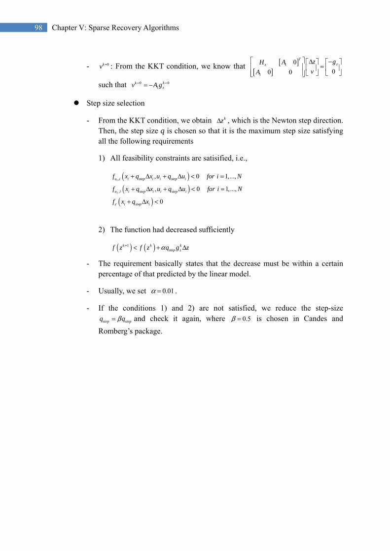
98 Chapter V: Sparse Recovery Algorithms
- 0kv = : From the KKT condition, we know that [ ][ ]
1
1
0
00 0
Tzz
z gH A
vA
Δ − =
such that 0 01
k kzv A g= == −
Step size selection
- From the KKT condition, we obtain kzΔ , which is the Newton step direction. Then, the step size q is chosen so that it is the maximum step size satisfying all the following requirements
1) All feasibility constraints are satisified, i.e.,
( )( )
( )
1
2
,
,
, 0 1,...,
, 0 1,...,
0
u i i step i i step i
u i i step i i step i
i step i
f x q x u q u for i N
f x q x u q u for i N
f x q xε
+ Δ + Δ < =
+ Δ + Δ < =
+ Δ <
2) The function had decreased sufficiently
( ) ( )1k k kstep zf z f z q g zα+ < + Δ
- The requirement basically states that the decrease must be within a certain percentage of that predicted by the linear model.
- Usually, we set 0.01α = .
- If the conditions 1) and 2) are not satisfied, we reduce the step-size
step stepq qβ= and check it again, where 0.5β = is chosen in Candes and
Romberg’s package.

99
99 4: Homotopy Algorithms
4. Homotopy Algorithms A. Motivation In this section, we aim to study the paper by Donoho and Tsaig [18] where the so-called Homotopy algorithm was proposed to solve the Basis Pursuit problem given in (97), the L1 minimization solution, i.e.,
1min x subject to y A x= . The motivation for studying this
algorithm includes: It is a fast algorithm perhaps suitable for large scale L1 minimization problems. As
Donoho and Tsaig comments (see the caption in Fig. 1 of [18] and the relevant
discussion in the body text) “Homotopy probably solves L1 minimization problem.”
It has the K iterative-step solution property. The K-sparse solution can be obtained in
K iterative steps when sufficient sparsity is present. This is interesting.
It is related to other algorithms such as Least Angle Regression (LARs), LASSO,
Orthogonal Matching Pursuit (OMP). OMP is probably the fastest; but it is superior
to the BP. There are cases where the OMP cannot find the sparse solution while L1
can.
The interior point methods, and many other conventional L1 norm minimization
routines, start at a dense solution and approach the sparse solution as iteration goes.
Meanwhile, the Homotopy and the OMP build a sparse solution through the iterative
steps by including or removing a sparse set of elements. If the solution is sparse, it is
easier to accept now, the Homotopy and the OMP must be faster and simpler than the
interior point methods. The complexity of Homotopy is O(K3+KMN).
The Homotopy method was originally proposed by Osborne, Presnell, and Turlach [21][22] for solving noisy over-determined L1 penalized least squares problem. Donoho and Tsaig [18] used it to obtain the sparse solution of underdetermined problem using the L1 norm minimization, i.e., the Basis Pursuit problem given in (97). B. The Homotopy Problem In the Homotopy problem, one aims to solve the following unconstrained L1 penalized least squares problem:
(Homotopy) 21
2 12min +
xy Ax xλ− (116)
The lambda is a utility variable, i.e., [ )0,λ ∈ ∞ . Given a fixed λ , we note, there is a
corresponding solution, say xλ . If the utility variable is varied, the solution traces a path.

100 Chapter V: Sparse Recovery Algorithms
There exists a set of solution paths { : [0, )}xλ λ ∈ ∞ . The desired L1 solution, we hope for,
shall be approached as we change the utility variable. In this case, it is changed from a large
value to smaller ones. See the illustration below.
Figure 7: Variation of the penalized objective function as lambda is changing from 4 to 0.
Why? Why not from a smaller value to larger values of lambda?
We note that a large λ can be used to put more emphasis on the L1 norm while for a smaller
λ the more emphasis on the L2 norm of the difference. Thus, for a large λ the solution xλ
shall be close to the zero vector. Smallness of x dominates the minimization result whether or
not such an x is a feasible solution. As 0λ → , we further note, the emphasis is put more on
the feasibility of the solution. At this point, it shall be nice to recall the nature of finding the
solution of the L1 norm minimization. We make the L1 ball to grow until it hits the feasibility
space for the first time. The first feasible solution at which the L1 ball touches the feasibility
space is the L1 norm minimized solution. Thus, it now makes a little more sense why we
-2 -1 0 1 2 3 4 5 60
5
10
15
20
25
30
35
40
x
||y - Ax||22 + λ ||x||1
λ → 0

101
101 4: Homotopy Algorithms
shrink the value of lambda started off from a large value. Thus, as λ shrink from a large
value to a smaller one, xλ converges to the L1 norm minimization solution, the solution of
the Basis Pursuit problem (97). It looks like starting from a solution closely satisfying
y Ax= .
LASSO: One can consider the following optimization problem, the so-called LASSO
problem, that Tibshirani [23] has proposed:
(LASSO) 2
12min s.t.
xqy Ax x ≤− (117)
where [0, )q ∈ ∞ and qx a solution in (117). The set of solutions { : [0, )}qx q ∈ ∞ identifies
a solution path 0qx = as the utility variable q is increased from 0q = . As q → ∞ , qx
converges to the solution of the Basis Pursuit problem (97). It seems that the two problems
are equivalent, LASSO and Homotopy, as there exists a reparametrization ( )q λ defined by
1( ) || ||q xλλ = so that the solution path of the Homotopy( λ ) and that of LASSO( ( )q λ )
coincide.
Osborne et. al [21] found that the solution path follows a polygonal path. Based on these
observation, the Homotopy algorithm is developed, which follows the solution path by
jumping from vertex to vertex of this polygonal path. Perhaps, the meaning of this will
become clearer after we have introduced the algorithm. For the moment, we can define the
meaning of the active set. The active set is defined as the index set of non-zero elements of x
at a particular iterative step of the algorithm. It starts at 0xλ = for a large λ with an empty
active set. At each vertex, the active set is updated through the addition or removal of “active”
elements. An active element here means the element which is believed to be an non-zero
element of the sparse vector x using the clues gathered up to that particular step in the course
of the algorithm. In a sequence of steps, the algorithm’s active set is guided to become the
support set of x as λ is made to go to zero in a controlled manner.
The following figure, Figure 8, taken from Donoho and Tsaig (Fig. 1 of [18]) illustrates the
position of Homotopy in the map of relations from L1 minimization, to Least Angle

102 Chapter V: Sparse Recovery Algorithms
Regression (LARs), and to the OMP algorithms:
Figure 8: Relation map of algorithms. From Donoho and Tsaig [18].
(1) Homotopy probably solves L1 minimization problems.
(2) LARS is obtained from Homotopy by removing the sign constraint check. (Not
removing an element from the active set.)
(3) OMP and LARS are similar in structure, OMP solves a least squares problem at each
iteration, whereas LARS solves a linearly penalized least-squares problem.
Theorem (The K-step Property of Homotopy). Let { }: max ,i ji j
a aμ≠
= where ia s are the
columns of the sensing matrix A. Let the sparsity of the vector x satisfy the following inequality
1( 1) 2.K μ−≤ + (118)
Then, the Homotopy algorithm runs K steps and stops, delivering the correct solution. Remarks: It is worthwhile to note that the sufficient condition (118) is identical to the sufficient condition that the solution of the BP problem is identical to the unique L0 norm minimization solution. In addition, Tropp [19][20] found that when (118) holds, even the OMP algorithm recovers the unique L0 solution. The OMP is a very simple greedy algorithm, which will be discussed shortly. In fact, when the degree of restrictiveness of the sufficient condition (118) is considered, namely it is so restrictive that even the simplest OMP algorithm finds the correct unique solution. The theorem of Homotopy algorithm is not at all surprising because it is more advanced and complex than the OMP algorithm. C. Two constraints from the subdifferential Let ( )fλ x denote the objective function of the Homotopy problem, i.e.,
21
12 2( ) : + || ||f x y Ax xλ λ= − . (119)

103
103 4: Homotopy Algorithms
We will solve this problem and obtain xλ as λ is started at a large value and varied while
converging to zero. At each time λ is varied, the selection should be carefully made. The selection criterion is derived from the classical convex analysis. From the classical convex analysis, a necessary condition for xλ to be a minimizer of
( )f xλ is that the zero vector is an element of the subdifferential of fλ at xλ , i.e.,
0 ( )x f xλ λ λ∈∂ , where
1( ) ( ) + || ||Tx xf x A y Ax x
λ λλ λ λ λλ∂ = − − ∂ (120)
and
,1
sgn( ), ( ) 0|| || .
[ 1,1], ( ) 0i iN
xi
u x x ix u R
u x iλ
λ λλ
λ
= ≠ ∂ = ∈ ∈ − =
Let { }: ( ) 0i x iλ= ≠ denote the support set of xλ . Let us refer to ( ) Tc A y A xλ= − as the
vector of residual correlations. Then, the condition 0 ( )x f x
λ λ λ∈∂ can be written equivalently as two conditions. The first
one is the sign agreement,
( ) sgn( ( )), c i x i iλλ= ⋅ ∀ ∈ . (121)
In words, on the support of , the residual correlation must all have magnitude equal to λ, and the sign of the corresponding element of xλ should match the sign of the residual
correlation. The second is the upper-bound on residual correlation,
{ }( ) , 0,1, , 1c i i Nλ≤ ∀ ∈ − (122)
It says that off the support of the residual correlation must have magnitude less than or equal to λ. The Homotopy algorithm carefully traces out the optimal path xλ that maintains the
conditions (121) and (122) for all 0λ ≥ . The key to its successful operation, as Donoho and Tsaig puts it, is that the path xλ is a piecewise linear path, along the vertices of a
polygon. D. The Homotopy Algorithm
Homotopy is an iterative algorithm. Similar to the Newton’s method, seen in the previous

104 Chapter V: Sparse Recovery Algorithms
sections, it finds the direction and the step-size. Then, the update of solution is made by
moving the current solution estimate by the amount of step-size in the found direction. One
notable aspect is that throughout its operation, the algorithm aims to maintain the active set I
{ }: ( )l lI j c j c λ∞
= = = (123)
which satisfies the conditions (121) and (122). As the iteration goes, the active set shall converge to the sparse support set . We would like to have the residual correlation be smaller each time.

105
105 4: Homotopy Algorithms
The Homotopy Algorithm ==================================================================
1. Initialize: Given A and y (= Ax), set 0 0x = , I = ∅ , 0Tc A y= , 0 0d = , IA = ∅ ,
and 0cλ∞
= . Let the iteration index be l = 0, 1, 2, …
2. Update direction:
Obtain an updated direction vector ld for the active set by solving
( ) sgn( ( ))TI I l lA A d I c I= (124)
Let ( ) 0cld I = .
(This direction update ld ensures that all the magnitudes of residual correlations on
the active set decline equally.)
3. Determine the step-size ls :
There are two cases of constraint violation (for the two constraints).
Case 1: A nonactive element of lc would increase in magnitude beyond λ, violating
the upper bound in (122). This first occurs when
( ) ( )
min ,1 ( ) 1 ( )c
l ll T Ti I
i I l i I l
c i c is
a A d I a A d I
λ λ+
∈
− += − + (125)
where the minimum is taken only over positive arguments. Call the minimizing index i + . Case 2: An active coordinate crosses zero, violating the sign agreement in (121). This first occurs when
( )
min( )l
l i Il
x is
d i−
∈
−=
(126)
where the minimum is taken only over positive arguments.
Call the minimizing index i − .
The step-size is determined as the minimum of the above two:
{ }min ,l l ls s s+ −= (127)

106 Chapter V: Sparse Recovery Algorithms
4. Update the active set, the solution estimate, the residual correlation, and λ .
{ } if
{ } otherwise.l lI I i s s
I I i
+ +
−
= ∪ = = −
1l l l lx x s d+ = +
1 1( )Tl lc A y Ax+ += −
1lcλ + ∞=
5. If residual correlation is zero, then stop; otherwise let 1l l= + and go to Step 2 :
This algorithm terminates when || || 0lc ∞ = , which indicates the solution has been
reached. ================================================================

107
107 4: Homotopy Algorithms
E. Proof of the Theorem There are introductory assumptions for the proof of the Theorem. 1. Let y Ax= with 0|| ||x K= and x has its nonzeros in the first K positions.
2. If two or more coordinates are candidates to enter the active set, assume the algorithm inserts them one at a time, on separate stages. 3. Let lx denote the Homotopy solution at the l th step, l lr y Ax= − the residual at the step,
and Tl lc A r= the corresponding residual correlation vector.
Definition (Correct Term Selection Property). The Homotopy algorithm has the Correct Term Selection Property at a given problem y Ax= , if at each iteration, the algorithm selects a new term to enter the active set from the support of x. If the Homotopy has the the Correct Term Selection Property, at the termination, the support set of the solution is guaranteed to be a subset of the support set of x. Definition (Sign Agreement Property). Homotopy algorithm has the Sign Agreement Property if at every step l for all j I∈ sgn( ( )) sgn( ( ))l lx j c j= .
That is, the Homotopy has the sign agreement property if, at every step of the algorithm, the residual correlations in the active set agree in sign with the corresponding solution coefficients. This ensures that the algorithm never removes elements from the active set. Lemma 1. The Homotopy algorithm has the K-step solution property if and only if it has the correct term selection property and the sign agreement property. Proof: Converse proof first. After K steps, correct term selection property implies that the active set is a subset of the support of x, i.e., {1, 2, , }I K⊆ . The sign agreement property ensures that no variable leaves the active set. Thus, after K steps, {1, 2, , }I K= , the Homotopy algorithm recovers the correct sparsity pattern. To show that the algorithm terminates at the K step, the step-size Ks is chosen so that, for some cj I∈ ,
( ) ( )TK K j I K K Kc j s a A d I sλ− = −
with ( )K Kc Iλ∞
= .
In addition, for the K th update, we have ( ) 1( ) T T
I K I I I I K KA d I A A A A r r−
= = since Kr is
contained in the column space of A (because k kr y Ax= − and y Ax= is noiseless.)
Hence, ( ) ( )c
c TK I KI
c I A A d I= and K Ks λ= is chosen to satisfy the sign agreement constraint.
Therefore, the solution at step K has KAx y= . Since y has a unique representation in terms of
the columns of IA , we conclude that kx x= .
Now let us do the forward part. It is obvious, since violation of either the correct term

108 Chapter V: Sparse Recovery Algorithms
selection property or the sign agreement property would result in a number of steps greater than k or an incorrect solution. Lemma 2. (Correct Term Selection) Let the sufficient condition of the Theorem holds, i.e.,
1( 1) 2.K μ−≤ + Let the residual at the lth step be written as a linear combination of the first
K columns in A, i.e., 1
( )k
l l jj
r w j a=
= . Then the next step of the Homotopy algorithm selects
an index from among the first K. Proof. We will show that at the lth step
1max , max ,l i l i
i K i Kr a r a
≤ ≤ >> (128)
and so at the end of the lth iteration, the active set is a subset of {1,2, , }K .
Let : TG A A= denote the Gram matrix of A. Let 1ˆ arg max ( )i K li w i≤ ≤= . The left-hand side
of (128) is bounded below by
ˆ1
ˆ,1
ˆ,ˆ
ˆ
max , ,
( )
ˆ( ) ( )
ˆ( ) ( )
ˆ ˆ( ) ( 1) ( )
l i l ii K
K
l i jj
l li jj i
l lj i
l l
r a r a
w j G
w i G w j
w i w j
w i K w i
μ
μ
≤ ≤
=
≠
≠
≥
=
≥ −
≥ −
≥ − −
(129)
since 22|| || 1ja = for all j and ˆ,
: max ,i ji j i jG a aμ
≠≤ = for ˆj i≠ . On the right-hand side of
(128), for i K> , we have
1
1
, ( )
( )
ˆ( ) .
K
l i l ijj
K
lj
l
r a w j G
w j
K w i
μ
μ
=
=
≤
≤
≤
(130)
Then, we note that (128) holds if the lower bound (129) is greater than or equal to the upper bound (130), i.e.,
1 ( 1) .K Kμ μ− − > (131)

109
109 4: Homotopy Algorithms
Recall that in the Homotopy algorithm the sign agreement condition (121) is used to remove an index i from the active set at stage l if the sign agreement condition is violated. The following lemma shows that, when x is sufficiently sparse, the sign disagreement never happens. Namely, at each stage of the algorithm, the residual correlations in the active set agree in sign with the direction of change of the corresponding terms in the solution. In other words, the solution moves in the right direction at each step. In particular, it implies that throughout the Homotopy solution path, the sign agreement property is maintained. Again this happens when when x is sufficiently sparse, i.e., 1( 1) 2K μ−≤ + . Lemma 3. (Sign Agreement) Suppose that y Ax= , where x has only K nonzeros, with K
satisfying 1( 1) 2K μ−≤ + . For {1, 2, , }l K∈ , let Tl lc A r= , and the active set I be defined
as in (123). Then, the updated direction ld defined by (12) satisfies
sgn( ( )) sgn( ( )).ld I c I= (132)
Proof: Let l lcλ∞
= . We will show that ( ) sgn( ( )) 1l lI I− <d c for i I∈ , which means that
(132) holds. From (12) and (9), we have ( ) ( ) ( ) ( )Tl I I d l l l lA A e d I d I c Iλ λ− = − + where de
is the identity matrix. This yields
( )
( )
( , )
( ) ( )
( )
1( )
21
( ) ( ) ( )2
1( ) ( )
2
l l l
TI I d l l
l l
l l l l
l l l l
d I c I
A A e d I
d I
c I d I c I
d I c I
λ
λ
μ λ
μ λ
μ λ λ
∞
∞∞ ∞
∞
∞ ∞
∞
−
≤ − ⋅
−≤
−≤ + −
−= + −
(133)
where ( , )∞ ∞
⋅ denotes the induced L∞ operator norm.
Rearranging terms, we get
1
( ) ( )1l l l l ld I c I
μλ λ λμ∞
−− ≤ ⋅ <+
and so
( ) sgn( ( )) 1l ld I c I∞
− < .
Thus (21) follows.

110 Chapter V: Sparse Recovery Algorithms
5. Bayesian Compressive Sensing on the Graph Model There are a number of approaches in the compressive sensing literature relevant to the title of this section. A few of the authors are Dror Baron and Baraniuk, Donoho, et. al (Donoho, A. Maleki, and A. Montanari), and others. Our approach in this section will be different from these other approaches, independently done. Our main focus in this section has been to Derivation of a Belief Propagation (Message Passing) algorithm which determines
the posterior probability on the signal values given the observation. In this regard,
our algorithm derivation is similar to that of Gallager for his probabilistic decoding
method of low density parity check code.
Derivation of the state distribution and the support set recovery algorithm. Once the
support set is recovered, the determination of the signal values will be done via
solving the over-determined Least Squares (LS) solution. This process enables early
breaking out of the costly iterative process.
Demonstration that the derived algorithm can be applied to real or complex valued
signals, quantized values and elements of the signals and the sensing matrix, as well
as to them over Galois field GF(q). Our preliminary results show that GF(q) results
well follow the prediction made by the Gilbert Varshamov bounds discussed in
Chapter VI.2.
Major research problems still remain include: Determination of the limit performance of this Bayesian approach, in comparison
with the sufficient conditions we have obtained in the previous sections.
Connections to the RIP conditions and the sufficient conditions to L1 unique solution.
Here the matrix is designed to be sparse, rather than the dense matrices often
assumed in the majority of compressive sensing literature. There exists an intriguing
relation between the density and the RIP constant.
Determination of the density of the sensing matrices (the number of non-zero
elements). There is a trade-off relation between the density and the performance.
Increasing the density, the minimum distance of the code grows, but the iterative
algorithm covered in this section shall not work very well. This is what we have

111
111 5: Bayesian Compressive Sensing on the Graph Model
learned from our coding theory class. There the values have been restricted to 1s and
0s. Here the alphabet is much larger, the set of real numbers. In the decoding process,
however, the alphabet is often quantized and discretized densities have been used for
iterations. Then, the question is to investigate the performance trade-off relation
between the quantization effect (noise) and the overall complexity. The other
approach is to use a high density sensing matrix and use a Gaussian approximation.
When there are many connections in the graph, a dense graph, a Gaussian
approximation may work out well. The trade-off here will be that since high density,
the matrix will have a large minimum distance, the spark, but the reconstruction
perhaps is just an approximation, rather than an exact recovery of the solution. This
is interesting research point which may have deep impact to the coding theoretic
practice of iterative message passing algorithms.
A. Iterative Compressive Sensing Algorithm There are two states: 0tS = or 1tS = for 0,1, , 1t N= − . The state tS is taken from the 0-
1 Bernoulli random variable with parameter KNp = where K is the approximate sparsity.
When the state is zero, the sample tx is taken from the zero state distribution, say2
0 0( ) (0, )f x σ ; or when the state is one, it is taken from the first state distribution, i.e.,2
1 1( ) (0, )f x σ . Roughly, therefore, there are K first states out of N positions. Now the problem is to determine the realization of the input vector ( )0 1 1Nx x x x −= given
the observation of the syndrome of the following parity check relation
P1:
00
11
11
1 0 0 100 10
11 1 0 00 0 1:
0 0 1 100 1 0
=: NM
xy
xyy
xy
F x−−
− − − − = = −
(134)

112 Chapter V: Sparse Recovery Algorithms
We now aim to design the iterative density passing algorithm. The purpose of the message passing algorithm is to obtain the distributions of the signal values 0 0P( | , )x Cτ= y and the those of the states { }Pr 1| ,tS r C= , use them to determine the
support set , the non-zero element states, by thresholding, say { } 12Pr 1| ,tS r C= ≥ . Once
all the non-zero states have been determined, the unknown values on each of the states can be determined by solving the over-determined Least Squares Estimate(LSE) of the unknown K-
sparse vector, i.e., ( ) 1T Tx A A A y−
= . When this estimation is good enough, i.e.
2r Ax δ− ≤ , a certain threshold, one can stop the iteration. A suitable threshold δ can be
determined from a probabilistic analysis. Obviously, the larger the threshold, the algorithm can stop earlier but the greater the inclination to errors. B. The Distribution of the Signal Value The decoding theorem is given here, which is given as an example to determine the first value 0tx = without loss of generality. Note that the first signal node 0x is connected to the
first observation 0y as well as to the second observation 1y . The first observation is then
connected to the signal nodes 3x and 6x ; the second one to 1x and 7x .
Theorem 1: The aposteriori probability that the first value, 0 0x τ= , takes a certain point in
s0 x0
s1 x1
s2 x2
s3 x3
s4 x4
s5 x5
s6 x6
s7 x7
+
+
+
+
y0
y2
y1
y3
Prior information is given p, ,
Figure 9: The Graph

113
113 5: Bayesian Compressive Sensing on the Graph Model
an alphabet , given the observation y and enforcing the checks (checks should be satisfied), is given by
( )( ) ( )
( )
0 00 0 0 0 0 0,0 0,0 0,0 0,0
0,0 0,0
1 0 0 0,1 0,1 0,1 0,1
0,1 0,1
|P( | , ) P | , , ( | )
|
P | , , ( | )
P xx C C x P
P C
C x P
ττ τ
τ
=
=
== = = = =
× = = =
x τ
x τ
yy x τ y x τ y
y
x τ y x τ y
(135)
We apply the same procedure and obtain a similar AP result for each 0τ in the alphabet. We
repeat this procedure for each element of the input vector x. Note that one can make a Maximum A Posteriori decision at any time given the posterior distribution for each element. Proof: Let us consider the following derivation to determine the distribution of the first value,
0x . Note that without loss of generality, we can repeat the same procedure for the rest of the
variables, tx s.
( )( )
( )( )
0 0 0 0 3 3 6 6 1 1 2 2 7 7
0,0 0,0 0,1 0,10,0 0,0 0,1 0,1
0 0 0,0 0,0 0,1 0,1
0,0 0,0 0,1 0,1
0 0 0,0 0,0 0,1 0,1
P( | , ) P( , , , , , | , )
P , , , ,
,
P | , , ,
,
x C x x x x x x C
x C
P C
C x
P C
τ τ τ τ τ τ τ
τ
τ
= = = =
= =
= = = = = = = =
= = ==
= = ==
x τ x τx τ x τ
x τ x τ
x
y y
x τ x τ y
y
x τ x τ y
y
( ) ( )( )
0,0 0,0 0,1 0,1
0 0 0,0 0,0 0,1 0,1
0 0 0 0,0 0,0 1 0 0 0,1 0,1
0,0 0,0 0,1 0,1
( , , | ) ( )
P | , , | , ,
|
P x P
C x P C x
P C
τ
τ τ
= =
= =
×
= = =
= = = == ×
x τ τ
x τ x τ
x τ x τ y y
x τ y x τ y
y
( )( ) ( )
0 0 0,0 0,0 0,1 0,1
0 00 0 0 0,0 0,0 0,0 0,0
0,0 0,0
( , , | ) ( )
|P | , , ( | )
|
P x P
P xC x P
P C
τ
ττ
=
= = =
== = = = ×
x τ
x τ x τ y y
yx τ y x τ y
y
( )1 0 0 0,1 0,1 0,1 0,1
0,1 0,1
P | , , ( | )C x Pτ=
= = =
x τ
x τ y x τ y
(136)
Q.E.D.

114 Chapter V: Sparse Recovery Algorithms
A single round of calculation of the posterior distribution { }P( | , ) :t t tx Cτ τ= ∈y for each and
every variable, 0,1, , 1t N= − , constitute a single iteration. We repeat the iteration again and again. In a single iteration, all N different posterior distributions are updated once. Why do we need iterations? Why can’t we be just satisfied with a single iteration? This has to do with our choice on the density of the sensing matrix. We have chosen sparse sensing matrix. Thus, the graph is sparsely connected. This is because that way the iterative algorithm works well. In one iteration, only local information is gathered. Through many iterations, the whole information available from the entire observation y and from the checking relations presented in the sparse graph, can be gathered. Enough number of iterations should be repeated before an attempt to make a Maximum A Posteriori (MAP) decision on the value of each signal node. One may choose to apply the MAP rule on the posterior distribution obtained at the end of a prescribed number of iterations. That is, we determine the value of each variable via the following rule
ˆ : arg max ( | , )t t tt
x P x Cτ
τ= = y (137)
for each t, 0,1, , 1t N= − .
Note that ( )0 0 0 0,0 0,0 0,0 0,0
0,0 0,0
P | , , ( | )C x Pτ=
= = =
x τ
x τ y x τ y is obtained from the convolution
of probability density functions for random variables x3 and x6. Similarly,
( )1 0 0 0,1 0,1 0,1 0,1
0,1 0,1
P | , , ( | )C x Pτ=
= = =
x τ
x τ y x τ y for all x0 is obtained from the convolution of
random variables x1, x2 and x7. The convolution operations can be computed in the frequency domain using FFT and IFFT. For clarity, we use the following examples. Example) From the system of equations y = Fx, we note that the first equation is
0 0 3 6x y x x= + + ; and the second equation is 0 1 1 2 7x y x x x= − + − .
00
11
11
1 0 0 100 10
11 1 0 00 0 1:
0 0 1 100 1 0 NM
xy
xyy
xy −−
− − − − = = −
Here 0y is an observed value; thus, a determined and given value. We know the distributions
of the random variables 3x , 6x , and those of 1x , 2x and 7x . We aim to find the
distribution of 0x that satisfies the two equations simultaneously. For the first equation, we
note that, the distribution of 0x is determined by the convolution of the distribution of 3x
and that of 6x . For the second equation, it is determined by the convolution of the
distributions of 1x , 2x and 7x : One may obtain the convolution of 1x , 2x first; and the
output of this convolution is convolved again with the distribution of 7x .

115
115 5: Bayesian Compressive Sensing on the Graph Model
C. The Distribution of the Signal Value in the Presence of Noise
We now consider a little bit different problem. We choose 2
0σ =0 in P1. Thus, the vector x is exactly sparse, which means that when the state is zero, the value of the variable node is zero with probability 1. In addition, the observation is made under the additive white Gaussian noise with zero mean and variance of 2
No where oN is the single sided power spectral
density of the noise. Now the problem is to determine the realization of the input vector ( )0 1 1Nx x x −=x given
the noisy observation of the syndrome of the following parity check relation
00 0
11 1
11 1
1 0 0 100 10
11 1 0 00 0 1:
0 0 1 100 1 0
=:
:
NM M
xr w
xr w
xr w−− −
− − − − = = + −
+= +
r
Fx w
y w
(138)
Theorem 2. The decoding theorem is given by the following equation. It is given as an example to determine the first value 0tx = without loss of generality. It is the result of the Maximum A Posteriori criterion which is used to determine the first value 0x :
0 0 0 0
0 0
P( | , ) P( | , , ) ( )
P( | , ) ( )
x C x C p
x C p
τ τ
τ
= = =
= = = −
w
w
r w r w
y r w w
(139)
The proof is obvious and omitted. We can use Theorem 1 to determine 0 0P( | , )x Cτ= = −y r w . Thus, the result can be obtained by averaging it over the distribution of the noise. D. Distribution of the Binary State Value
Since there are only two states, it might be more robust to determine the state at each node,
instead of the exact value tx . Once the states are found, the over-determined problem can be
solved, and the unknown sparse vector x can be found.
Given the distribution 0 0P( | , )x Cτ= r , there are number of ways we can obtain the LLRs for
the state likelihoods.
1. Use the Kulback-Leibler Distance to the distribution of the zero state probability, i.e., ( )0 0P( | , ) || ( )D x C f xr and to that of the non-zero state probability, i.e.,

116 Chapter V: Sparse Recovery Algorithms
( )0 1P( | , ) || ( )D x C f xr . Compare the result and determine the state value.
2. Find the probability of the state value given the prior distribution and the posterior
0P( | , )x Cr . We are given from the problem set up the conditional probability distribution
{ }0 0 0| 0 ( )p x S fτ τ= = = and { }0 0 1| 1 ( )p x S fτ τ= = = , and the prior distribution on the
state values, namely, the state tS is the 0-1 ( )Bernoulli KNp = , i.e. { }0Pr 1S p= = . Next
suppose that observation r is made, and the posterior distribution 0( | , )p x r Cτ= has been
obtained by enforcing the parity-checking relations to r. Now, we ask
{ } { }
{ } { }0 0 0 0
0 0 0
: Pr 1| , 1, | ,
Pr 1| , , | ,
S r C p S x r C d
S x r C p x r C d
γ τ τ
τ τ τ
= = = = =
= = = =
(140)
We note the term { }0 0Pr 1| , ,S x r Cτ= = . It is equal to { }0 0Pr 1|S x τ= = once the value
0x is given, r and C do not provide any additional information to the state value.
Now, let us work on the conditional probability { }0 0Pr 1|S x τ= =
{ } { }
( ) ( )( )
( )( ) ( ) ( )
0 00 0
0
0 0 0
0
1 0
1 0 0 0
Pr 1,Pr 1|
Pr{ }
| 1 Pr 1
1
KN
K KN N
S x dS x
x d
p x S S
p x
f x
f x f x
τ ττ
τ ττ
ττ
τ τ
= = += = =
= += = =
==
==
= + − =
(141)
Finally, one can design the decision maker, i.e.,
00
1, if 0.5Binary State Decision:
0, o.w.S
γ ≥=
(142)
Theorem 3. (The Posterior Binary State Distribution) Let tS is the 0-1 ( )Bernoulli KNp = .
Let the conditional probability distribution on the signal values at different states be { }0 0 0| 0 ( )p x S fτ τ= = = and { }0 0 1| 1 ( )p x S fτ τ= = = respectively. Let { }| ,tp x r Cτ=
be obtained from the message passing algorithm given by Theorem 2. Then, the probability of state tS , 0,1, , 1t N= − , given r and applying the check relation C, is obtained as
{ }( )
( ) ( ) ( ) { }1 0
1 0 0 0
: Pr 1| ,
| ,1
t t
KN
tK KN N
S r C
f xp x r C d
f x f x
γτ
τ ττ τ
= =
== =
= + − = (143)

117
117 5: Bayesian Compressive Sensing on the Graph Model
for 0,1,2, , 1t N= − . Support Set Recovery with Log Likelihood Ratios We note that { }Pr 1 | ,tS r C= may not be a probability measure given that
{ } { }Pr 1 | , Pr 0 | ,t tS r C S r C= + = is not equal to zero. This may be due to the approximation
we have made in (140) for { }0 0Pr 1 | , ,S x r Cτ= = , with { }0 0Pr 1 |S x τ= = (141).
To resolve this issue, one may use normalization. The other approach is to use the log ratio. We may opt to use the log ratio because the algorithm may be simplied with the log-ratio approach. Let us see.
{ }{ }
( )( ) ( ) ( ) { }
( ) ( )( ) ( ) ( ) { }
( ) { }( ) ( ) { }
00
0
1 00
1 0 0 0
0 00
1 0 0 0
1 0 0
0 0 0
Pr 1 | ,LR( ) : log
Pr 0 | ,
| ,1
log1
| ,1
| ,log
1 | ,
KN
K KN N
KN
K KN N
KN
KN
S r CS
S r C
f xp x r C d
f x f x
f xp x r C d
f x f x
f x p x r C d
f x p x r C d
τ τ ττ τ
τ τ ττ τ
τ τ τ
τ τ τ
==
=
==
= + − ==
− ==
= + − =
= ==
− = =
Note that it is in the form of log-sum-product. Express the integral operation as the Riemann summation. Then, we have
( ) { }( ) ( ) { }
1 0 0
0 0 0
1, 0,
| ,log
1 | ,
log log exp( ) log exp( )
KN
KN
f x p x r C d
f x p x r C d
Klp lp
N K τ ττ τ
τ τ τ
τ τ τ
= =
− = =
= + − −
where
( ) { }( )( ) { }( )
1, 1 0 0
0, 0 0 0
log | ,
log | ,
lp f x p x r C
lp f x p x r C
τ
τ
τ τ
τ τ
= = =
= = =
.
Note that the argument inside the logarithm is the product of two probability measures; thus, log of the product should be negative. Now, let us discuss one of the log products
( ) { }( )( )( ) { }( )
1, 1 0 0
1 0 0
log | ,
log log | ,
lp f x p x r C
f x p x r C
τ τ τ
τ τ
= = =
= = + =
.

118 Chapter V: Sparse Recovery Algorithms
Giving attention to the second term, we have
{ }( ) ( )( )
( )
( )
0,0 0,0
0,1 0,1
00
0 0 0,0 0,0 0,0 0,0
1 0 0,1 0,1 0,1 0,1
|log | , log
|
log P | , , ( | )
log P | , , ( | )
P xp x r C
P C
C x P
C x P
ττ
τ
τ
=
=
== =
+ = = =
+ = = =
x τ
x τ
y
y
x τ y x τ y
x τ y x τ y
Now, we note that the second and the third term are in the form of log-sum-product again. Let us find a way to simplify them. First, let us use the FFT technique to get rid of the cumbersome convolution operation. Recall that convolution in the time domain (the pdfs in this problem) is equivalent to the multiplication in the frequency domain (the product of characteristic function). We may apply the FFT technique to express the convolution. For example, the first term is the convolution of two random variables 3x and 6x , i.e., 3 6 0x x y τ+ = − . Let us denote
the FFT and IFFT operators as F and IF. Then, the pdf of the convoluted random variable is obtained by
( ) ( )( )=
= ×3,6 3 6
3 3 6 6
( ) *
IF F F ( )
pdf t pdf pdf
pdf pdf t (144)
Then, substitute 0t y τ= − and we have
{ }( ) ( )( )0
0 3,6 0 1,2,7 1
|log | , log log ( ) log ( )
|
P xp x r C pdf y pdf y
P C
ττ τ τ
= = = + − + −
y
y.
Now, substitute the result to the previous expression:
( ) { }( )( )( ) ( )
( )
1, 1 0
01 0 3,6 0 1,2,7 1
log | ,
|log log log ( ) log ( )
|
tlp f x p x r C
P xf x pdf y pdf y
P C
τ τ τ
ττ τ τ
= = =
= = = + + − + −
y
y
Similarly we have

119
119 5: Bayesian Compressive Sensing on the Graph Model
( ) { }( )( )( ) ( )
( )
0, 0 0 0
00 0 3,6 0 1,2,7 1
log | ,
|log log log ( ) log ( )
|
lp f x p x r C
P xf x pdf y pdf y
P C
τ τ τ
ττ τ τ
= = =
= = = + + − + −
y
y
Combining the results so far, we have
{ }{ }
{ } ( )
{ } ( )1
0
01, 0,
0
1, 1 1,max index
:max
0, 0 0,
:max
Pr 1| ,log log log exp( ) log exp( )
Pr 0 | ,
log max log 1 exp max
max log 1 exp max
S r C Klp lp
S r C N K
Klp lp
N K
lp lp
τ ττ τ
τ τττ
τ ττ
≠
=
=
= = + − = −
= + + + − − −
− − + − −
max indexτ ≠
Now, it becomes very simple to do the operation.

120 Chapter V: Sparse Recovery Algorithms
E. Useful Mathematical Identities for Log-Sum-Products Product of real numbers
( )sgn( )exp logi i iii i
a a a = ∏ ∏
An example is sgn( )sgn( )exp log logab a b a b= + .
A logarithmic identity We may use the following identity on the log sum of more than two numbers for positive numbers A, B, and C,
( )
( ) ( )
( ) ( )
log log(exp(log ) exp(log ) exp(log ))
log(e e e )
log(e (1 e e ))
log(1 e e ).
a b c
a b a ca
a b a c
A B C A B C
a
− − − −
− − − −
+ + = + +
= + += + += + + +
(145)
where it is supposed that max( , , )a a b c= .

121
121 0:
F. The Message Passing Algorithm The message passing algorithm is given as the following:
1. Initialization: Set ( ) ( ) ( ) ( )1 0| 1K K
t t t t t tN NP x f x f xτ τ τ= = = + − =y for all t. Determine a
threshold δ for stopping criterion.
2. Run message passing routine: Do the convolution (or the FFT/IFFT) routine for each t,
obtaining P( | , )t tx Cτ= y for all t.
3. Run the active set recovery routine. An index t will be decided to be added to the active if
the log ratio, ( )tLR S , for 0,1,2, , 1t N= − , is greater than zero, i.e.,
( ){ }: 0.0tI t LR S= >
4. Check if I is : Run ( ) 1T TI I I Ix A A A y
−= . When this value is good enough, i.e.
2r Ax δ− ≤ the threshold, the iteration can be put to stop. Otherwise, return to step 2
and repeat.
G. Donoho’s message passing algorithm for compressed sensing
Donoho et al. discuss a new iterative algorithm which builds upon a standard linear programming (LP) based iterative algorithm. According to the authors, this new algorithm brings dramatically faster reconstruction than the LP-based approach. The idea for improvement seems to be partly borrowed from the iterative message passing algorithm on bipartite code graphs popularly used in the coding theory community (They refer to Richardson and Urbanke’s Modern Coding Theory, Cambridge University Press, 2008). One key difference could be the addition of a corrective term to the iterative algorithm. Research in this direction shall be very interesting. Reference 1. D. L. Donoho, A. Maleki, and A. Montanari, “Message-passing algorithms for compressed
sensing,” vol.106, no.45, Proceedings of National Academy of Science, Nov. 10, 2009.

122 Chapter V: Sparse Recovery Algorithms
6. The Expander Graph Approach
In previous sections, we have demonstrated that the solution to the under-determined linear system of equations could be found using the L1 optimization approach, which has been known in the literature as “basis pursuit”. While L1 optimization can be done in polynomial-time (often 3( )O N ), this may still be infeasible in applications where N is quite large. In [1], motivated by the existence of bipartite expander graphs [6], a new scheme for compressive sensing with deterministic performance guarantees based on expander graphs was proposed. The recovery complexity of this algorithm is ( )O K , where K is the number of non-zero entries in the signal vector. Research in this direction shall be of interest.

123
123 7: Section References
7. Section References [1] Sina Jafarpour , Weiyu Xu , Babak Hassibi, and Robert Calderbank, “Efficient and
robust compressed sensing using optimized expander graphs” IEEE Transactions on Information Theory, 55 (9). pp.2009.
[2] W.Xu and B.Hassibi, “Efficient compressive sensing with deterministic guaratees using expander grahs,” Proceedings of IEEE Information Theory Workshop, Lake Tahoe, 2007.
[3] W.Xu and B.Hassibi, “Further results on performance analysisi for co-mpressive sensing using expander graphs,” Conference Record of the Forty-First Asilomar Conference on Signal, Systems and Computers. ACSSC 2007.4-7 Nov.2007 Pages(s):621-625,2008
[4] E. Candes, J. Romberg and T. Tao, “Robust Uncertainty Principles: Exact Signal Reconstruction from Highly Incomplete Frequency Information”, IEEE Transactions on Information Theory , 52(2) pp.489-509,Feb.2006.
[5] E. Candes and T .Tao, “Near Optimal Signal Recovery From Random Projections: Universal Encoding Strategies?”, IEEE Trans.on Information Theory, 52(12) pp. 5406 - 5425, Dec. 2006.
[6] Michael Sipser and Daniel A. Spielman “Expander codes”, IEEE Transactions on Information Theory , vol.42, NO.6,Nov,1996.
[7] L.A. Bassalygo and M.S. Pinsker, “Complexity of an optimum nonblocking switching network without reconnections”, Problems in Information Transmission, vol 9 no 1, pp. 84-87, 1973.
[8] Fan Chung and Linyuan Lu, “Concentration inequalities and martingale inequalities: A survey”, Internet Mathematics Vol.3,No.I:79-127.
[9] E. Candes and T. Tao, “Decoding by Linear Programming”, IEEE Trans. on Information Theory, 51(12), pp. 4203 - 4215, Dec. 2005.

124 Chapter V: Sparse Recovery Algorithms
8. Chapter Problems
Design a small scale y = Ax problem. The dimension of y should be at least 100 by 1. The
dimension of A should be 100 by 200. The unknown x should be a K-sparse vector. Let K
= 10. A is randomly generated from the Gaussian distribution. Make sure that the columns
of A have energy 1 by normalizing each column.
6. Consider the linear program given in class. Namely, it is
[ ]
[ ]
[ ]
[ ]
( , )min = 1 0 0 1
s.t. e e 0,
e e 0,
0 e 0,
0 0
T T T Tix u
i
xu u x
u
xx u
u
xx u
u
xu
u
xA b
u
+ =
− = −
− − = −
− = −
− =
a. Use the MATLAB’s standard routine to obtain the solution of linear program
solution. Keep it for reference.
b. Note that the constraint includes the non-negativeness of u. The programs in
L1-magic package by Candes and Tao do not include this. Seeing the effect of
including this term is one of our objectives.
c. Use the Lagrange-dual interior point method to do the L1 minimization.
First obtain the KKT conditions. Write them down.
d. Next obtain the Jacobian matrix discussed in class. Specify each and every
component matrices. Specify their dimensions.
e. Construct the two equations, one for λΔ and the other for ( ),x vΔ Δ .
f. Construct the Netwon’s step routine. Verify its correct operation by doing a
small problem of your own with known solution. Explain how you have verified
its correct operation. Include the verification results.
g. Implement the step-size selection routine in MATLAB. Complete the

125
125 8: Chapter Problems
MATLAB program implementation by including the stopping condition.
h. Verify the operation of your algorithm by solving the small scale problem.
i. Provide the evidence of the convergence of the solution estimate. Show the
duality gap narrows as iteration goes on. Show that the mean square error
between the solution estimate and the true solution narrows as the iteration goes
on.
7. Repeat the first problem with the Log-Barrier method.
a. Obtain the Hessian by specifying the compoment matrices. Specify their
dimensions.
b. Construct the matrix vector equation with the unknown ( ),x vΔ .
c. Implement the Netwoen method routine in MATLAB.
d. As done in the first problem, provide the evidence that your program is
working properly by making comparison with the first examples.
8. Repeat the first problem with the Homotopy algorithm. Do the full verification as to
show that your algorithm is working properly.
9. Compare the recovery performance of the four algorithms: the MATLAB’s built-in
routine, the primal-dual interior point method, and the log-barrier method. To compare,
do a Monte carlo simulation in which the sensing matrices are randomly generated and
the sparse-signals are randomly generated. Fix the matrix size as 100 x 200, try to see
the performance as you increase the sparsity K = 10, 20, 30, 40, 50.
10. Use the Bayesian method and verify your routine. Include into the comparison.
11. Use the log-barrier algorithm for SOCPs and solve TV1 Problem. Do the Shepp-Logan
phantom example. For this, refer to page 9 of the l1-magic program manual provided
by Candes and Romberg.

126 Chapter VI: Recent Research Results
Chapter VI. RECENT RESEARCH RESULTS 1. Deterministic Matrix Design This part will be added soon.
2. Coding Theoretic Approach This section is adopted from [8] (Section Reference). Compressed sensing has provided
a new signal acquisition framework with which one can take samples of a given signal of interest while compressing it simultaneously. This compressed sample taking is done via linear projection of the given signal against a prescribed set of kernels, i.e., one linearly projected sample per kernel. In its standard form, this compressed sensing operation is developed over the field of real numbers. In this presentation, we are interested in the development of compressed sensing over the finite fields. Fundamental limits on sensing measurement requirements as we vary the size of the finite field will be discussed. When compressed sensing is put to work in digital systems, the signals and the kernels should be represented in a finite precision manner anyhow; thus, the study of compressed sensing over finite fields should be of interest for implementation point of view. We aim to present our understanding on compressive sensing via Gilbert Varshamov (GV) bounds, new results on average spark calculation results, and proposal of the a posteriori (AP) signal recovery algorithm, and provide discussion on how they are related with each other.
We make note of existence of a few prior studies relevant to the content of this section. Draper and Malekpour [2] have studied compressed sensing over finite fields and obtained fundamental bounds on sensing requirements using the error exponent analysis techniques of the channel coding theory. Ardestanizadeh, Cheraghchi, and Shokrollahi [6] have studied the question how much bit precision on the compressive measurements will be needed for good recovery of sparse signals of a finite size alphabet, say q . They assumed the use of Vandermonde frames [5] and obtained that the precision requirement is 2
2( log log )NKO K q K+ .
Zhang and Pfister [4] discussed the connection between compressed sensing and error correction codes, and proposed the use of low density parity check matrices over GF(q) and a verification based iterative decoding schemes.
A. Compressed Sensing via Syndrome Decoding In this section, we aim to draw analogy between parity checking in coding theory and
the under-determined equation in compressed sensing by recasting the basic compressed sensing equation
y F x= (146)

127
127 2: Coding Theoretic Approach
as a coding theoretic parity-checking equation. Treat y as an 1M × syndrome vector, F as an M N× parity check matrix, M N< , and x as an 1N × K-sparse error vector. Note that this model is valid for real, complex, and finite fields GF(q). Finite fields can be useful for implementing the CS system in digital forms, with a finite precision representation, say
2log ( )q bit precision, done to the coefficients of the elements of the sensing matrices and signals.
We assume that K t≤ where t means the number of errors a given code defined by an F can correct. Let U = N – M. The rate R of the code is U/N. We can then find the N U×generator matrix G from F using the relationship that FG = 0 (e.g. using Gaussian elimination on F) where 0 denotes the M U× all zero matrix. Let be the codebook—collection of all
codewords. Each 1N × codeword c can be generated by multiplying an arbitrary 1U ×message vector m to the generator matrix, i.e., c Gm= . We assume c is sent over a noisy channel where the noisy channel introduces an additive random error pattern x to c, and the output of the channel is z = c + x.
In this setting, parity checking on z shall return the zero syndrome, i.e.,( )y F z F c x F x= = + = , unless there is zero errors or the error pattern x is a codeword, i.e.
x∈ ; otherwise it will give a non-zero syndrome vector. The code is linear and hence it contains the all-zero codeword. The error correction capability of this code can be parameterized by its minimum distance dmin. The minimum distance dmin is the minimum Hamming weight (the number of non-zero coefficients) of any codeword, since the code is linear, i.e.,
min0,
min ( )Hc c
d w c≠ ∈
c
. (147)
But a codeword is a word that satisfies the parity check equation, i.e., 0F x = . From this
observation, we may also write that mind is also the smallest number d that there exists a set
of d columns of a matrix F that are linearly dependent; this definition is the same as that of the spark in compressed sensing. This discussion will continue further in Section B. From the coding theory, we note that, a code defined by its parity check matrix F with dmin can correct all t or smaller error patterns, and t is given by
min min12 2
d dt − = ≈ . (148)
Our discussion up to (148) implies that all K-sparse error vectors x can be uniquely determined from the syndrome equation y = F x as long as K t≤ . Notice that this is a deterministic guarantee, rather than probabilistic, on the recovery of the sparse vectors. Such a code or a matrix F with dmin can be constructed. Namely, we can construct an F so that any collection of less than or equal to dmin – 1 columns of F is linearly independent. This means that dmin - 1 can be as large as the rank of F which is further upper bounded by M since M < N. Hence, we have the Singleton bound,
min 1d M− ≤ . (149)
Those codes that achieve the Singleton bound with equality are called maximum distance

128 Chapter VI: Recent Research Results
separable codes. They include the repetition codes and Reed Solomon (RS) codes. Real- or complex-valued RS code like sensing matrix F with dmin can also be found. The examples are given in [5],[7]. From (149), we can obtain min 1
2 2 2dM
N N N≥ + , by dividing both sides by 2N. By
defining the compression ratio Mcomp Nρ and the error correction ratio (ECR) t
t Nρ , we have
2comp tρ ρ≥ . (150)
We call (150) the CS Singleton bound. Any x whose sparsity ratio Ksp Nρ is smaller than
or equal to ECR (i.e., K t≤ ), can be uniquely determined from syndrome y. Fig. 1 shows the CS Singleton bound.
On the other hand, the Gilbert-Varshamov bound tells us the existence of a t error correcting linear block code. The rate R of such a code is given by,
( ) 1 ( )qR Hδ δ≥ − (151)
where mindNδ , N M
NR −= and ( )qH δ is the q-ary entropy function. It is the lower bound
on the rate required to have the relative minimum distance δ . Eq. (151) can then be written as,
(2 )comp q spHρ ρ≤ (152)
for [0,0.5]spρ ∈ .
It is interesting to note that (2 )q spH ρ approaches the line with slope 2 as q increases.
The required code rate can be as large as what this lower bound predicts for a long block length. It is then an upper bound on the redundancy. The number of check equations required for a sensing matrix to have the relative minimum distance is at most what this bound can tell us. One needs at most this much redundancy to be able to find a sensing matrix with the relative minimum distance δ . It can be shown that an ensemble of parity check (PC) codes, say ( , , , )s cN d d q block codes of length N, check degree cd , signal element degree sd , and
GF(q), closely approach the GV bound from above as the degrees are increased. Thus, GV bounds in fact work as a benchmark, instead of upper bounds. The check degree and the signal element degree indicate the number of non-zero entries in any row of a sensing matrix and the number of non-zero entries in any column respectively. We focus on the cases here that the degrees are fixed for each row and column. Thus, for a compressed sensing system with a large fieldGF( )q , the sufficient condition is going to approach
2comp spρ ρ>
. (153)
This means that if 2comp spρ ρ>
, a good sensing matrix exists and thus one can be found. As the
dimension of the system approaches infinity, a randomly selected code out of an ensemble will behave as good as what these bounds can predict, with probability getting close to 1.

129
129 2: Coding Theoretic Approach
Figure 10 : Gilbert-Varshamov Compressed Sensing Bounds for Sensing Matrices over GF(q) and The Singleton Bound B. The Sparks of Sensing Matrices over GF(q)
In this section, we aim to find the ensemble average sparks of an GF(q) LDPC codes. The spark of an M N× matrix is the smallest number S such that there exists a set of S columns of the matrix that are linearly dependent. One should note that spark for a sensing matrix and dmin for a parity check matrix are exactly the same. From the Singleton bound, then, 1S M− ≤ . Finding the SPARK of a sensing matrix is of paramount importance in compressed sensing because it can provide a limit on how sparse a signal has to be for guaranteed unique recovery. For example, if the spark of a certain M N× sensing matrix F is given to be S, then any signal x with the sparsity K can be uniquely determined from the combinatorial L0 minimization routine, as long as 2
SK ≤ . That is, 2SK ≤ is the sufficient
condition for the L0 norm minimization solution, subject to y = F x constraint, to return the unique solution. Otherwise, say 2 1SK = + for example, the solution is not unique, which can
be easily proved. The L0 minimization is known as an NP-hard problem since it is combinatorial. The sufficient condition, thus, provides a meaningful benchmark on the required sparsity.
Finding the spark of a matrix is thus desired, but it requires a combinatorial search and hence is an NP-hard problem by itself. In this section, we find the average spark of an ensemble of sensing matrices. For a system with a large block length N, the average spark of an ensemble of sensing matrices is very close to the spark of an individual sensing matrix randomly selected out of the ensemble. That is, it can be shown that the spark of an
0 0.1 0.2 0.3 0.4 0.50
0.1
0.2
0.3
0.4
0.5
0.6
0.7
0.8
0.9
1
Error Correction Ratio ρt (>ρsp)
Com
pres
sion
Rat
io ρ
com
pFundamental Bounds on Compressive Sensing
GV q=2GV q=4GV q=16GV q=256Singleton

130 Chapter VI: Recent Research Results
individual sensing matrix concentrates around the ensemble averaged spark. Theorem 1 : The average spark of an ensemble of GF(q) random sensing matrices, i.e.,
( , , , )s cN d d q , is given by
{ ( ) ( ) ( ) }SPARK( , , , ) min {2, , } 1 ln( 1) ln 0dNd
Ns c v sN d d q d N d d q d= ∈ − − + ≥ (154)
where the variable dN is a function of the check degree cd and it is given by
= Coeff ( ) c
N
dd dN p x
(155)
where0
( )cd
ii
i
p x p x=
= , ( )icd
ip = , for even i , 0i
p = for odd i, 0 ci d≤ ≤ , ( )Coeffd ⋅ denotes
the coefficient of the term dx in the expansion of the argument polynomial, and we assume
c
Nd is integer.
C.
Signal Detection Algorithms In this section, we aim to discuss how to detect the sparse signal x measured from a
sensing matrix F selected randomly out of an ensemble ( , , , )s cN d d q [3].
The sparse signal values can be obtained by solving the following problem:
GF( )
: arg max ( | , ) s.t. = t
t t tq
x P x y C y F xτ
τ∈
= = (156)
where 0,1, , 1t N= − and the symbol “C” in the conditioning argument compartment means satisfaction of all the M “check” relations. The function ( | , )t tP x y Cτ= is the
posterior distribution, given the observation, and after enforcing the check relations. This posterior distribution is updated for each element of the signal x. Theorem 2: The aposteriori probability (AP) that the first value, 0 0 GF( )x qτ= ∈ , given the
observation y and enforcing the checks (checks should be satisfied), is given by
( )( )
( ),
0 , 0,01
|P( | , )
|
| , , ( | )c
p
t p
tt
d
i t t pp x
P x yx y C
P C y
P C x x y P x y
ττ
τ=
== = ×
=
∏
(157)
We apply the same procedure and obtain the AP result for each element of x. A single round of calculation of the posterior distribution { }P( | , ) :t t tx Cτ τ= ∈y for each element,
0,1, , 1t N= − , constitutes a single iteration. In a single iteration, therefore, all N different posterior distributions are updated once. We repeat this iteration multiple times. Why do we

131
131 2: Coding Theoretic Approach
need iterations? Why can’t we be satisfied with a single iteration? This has to do with our choice on the density, controlled by the two degrees, of the sensing matrix. Choosing a sparse sensing matrix (small degrees) would be desired because when the matrix is sparse, the iterative algorithm works well from the experience we had on the low density parity check codes. In a single iteration, only local information is gathered because of sparse connections. Through iterations, it is hoped that and thus the algorithm is only sub-optimal, the entire information from observation y available via enforcing checking relations prescribed in the sparse matrix can be gathered. An enough number of iterations should be repeated before convergence can be seen on the value of each signal element.
It can be shown that the check posterior results, i.e.,
( ),
0 , ,| , , ( | )p
t p
i t t p t px
P C x x y P x yτ= in (157), can be obtained from a series of convolution
operations of the probability distribution functions of the signal variables connected to the pertinent check
piC . For example, suppose tx is connected via its first check to say x3 and
x6, then it is the convolution of the two distributions, one for the signal element 3x and the
other for 6x . The convolution operations can be conveniently done in the frequency domain
using FFT and IFFT. In [3], a couple of ideas on iterations based on identifying the support set detection are
also included. One of them is aiming to obtain the posterior distribution of the state tS of t
-th signal element. A state value tS is binary, 1 for the non-zero value of tx , and 0 for the
zero values. Then, the state posterior either Pr{ 1| , }tS y C= and Pr{ 0 | , }tS y C= can be
updated in each iteration. The log ratio of the posterior probabilities on the state is maintained in each iteration. For the state posterioir calculation, the prior information that the signal is sparse is utilized. When the log ratio is greater than 0, then the pertinent state is more like to be 1; otherwise it is zero. At the end of each iteration, we can determine the non-zero states by thresholding the log ratios, collect the indices of non-zero states, and form an estimate of the support set. Once a support set estimate of size K is given, one can then attempt to solve the over-determined problem (by collecting only those columns of matrix F and those elements of x corresponding to the non-zero indices) and find a solution x . If this one is found to satisfy the observation, i.e. y F x= , i.e., it is declared to be the solution; then the iteration can stop.
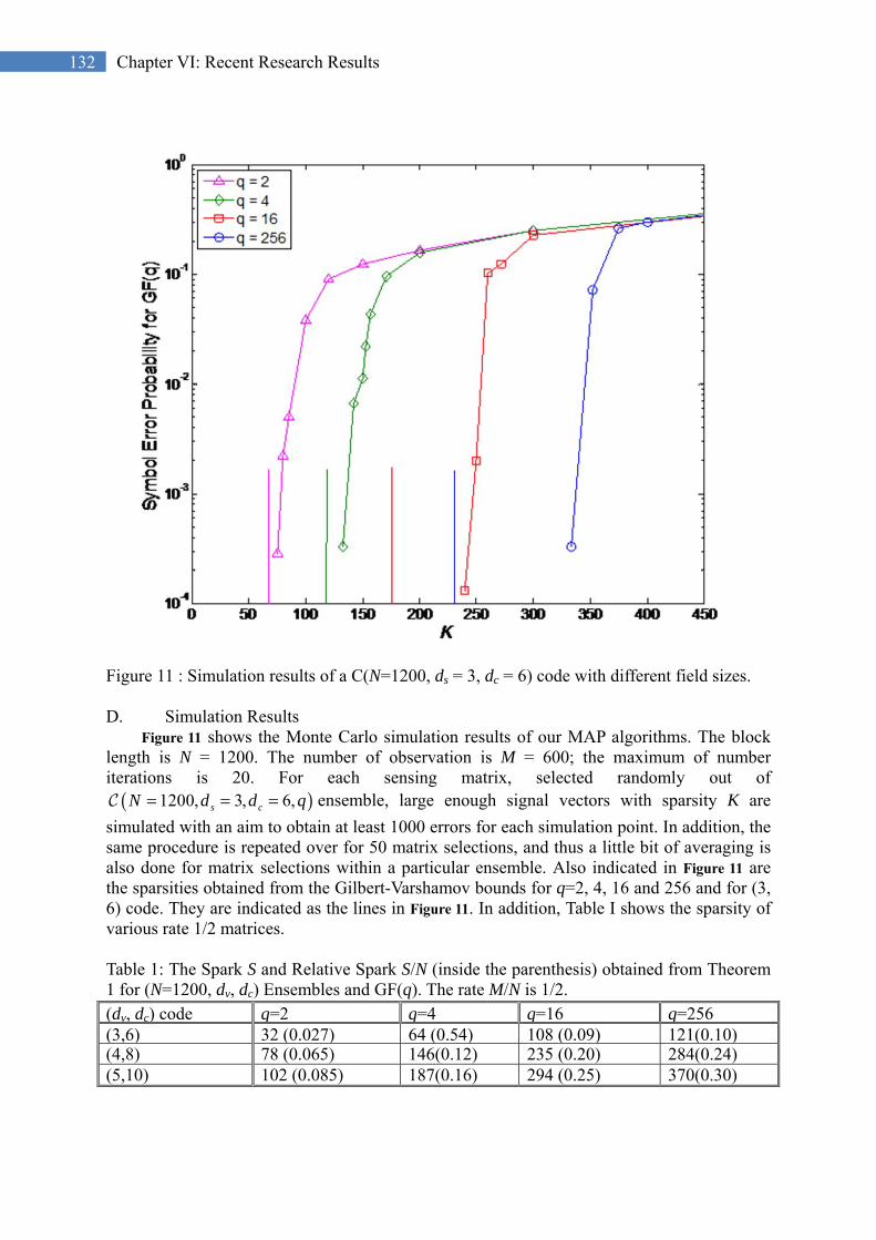
132 Chapter VI: Recent Research Results
Figure 11 : Simulation results of a C(N=1200, ds = 3, dc = 6) code with different field sizes. D. Simulation Results
Figure 11 shows the Monte Carlo simulation results of our MAP algorithms. The block length is N = 1200. The number of observation is M = 600; the maximum of number iterations is 20. For each sensing matrix, selected randomly out of
( )1200, 3, 6,s cN d d q= = = ensemble, large enough signal vectors with sparsity K are
simulated with an aim to obtain at least 1000 errors for each simulation point. In addition, the same procedure is repeated over for 50 matrix selections, and thus a little bit of averaging is also done for matrix selections within a particular ensemble. Also indicated in Figure 11 are the sparsities obtained from the Gilbert-Varshamov bounds for q=2, 4, 16 and 256 and for (3, 6) code. They are indicated as the lines in Figure 11. In addition, Table I shows the sparsity of various rate 1/2 matrices.
Table 1: The Spark S and Relative Spark S/N (inside the parenthesis) obtained from Theorem 1 for (N=1200, dv, dc) Ensembles and GF(q). The rate M/N is 1/2. (dv, dc) code q=2 q=4 q=16 q=256 (3,6) 32 (0.027) 64 (0.54) 108 (0.09) 121(0.10)(4,8) 78 (0.065) 146(0.12) 235 (0.20) 284(0.24)(5,10) 102 (0.085) 187(0.16) 294 (0.25) 370(0.30)

133
133 2: Coding Theoretic Approach
E. Section Summary We note that all three measures, the sparsity obtained from GV bounds, the ensemble average sparsity obtained from Theorem 1, and the simulation results of the iterative recovery algorithm, agree to the observation that as the field size q increases, a given sensing matrix of rate 1/2 can have large spark and thus can be used to detect the signals with a larger sparsity K. Simulation results show that the iterative algorithm can far surpass the predictions made by the average sparks as well as by the GV bounds, which is very interesting, and calls for further study. We also note that as the field size is increased, the compressed sensing bound is
2M K≥ for unique recovery under the Singleton bound. A sensing matrix that satisfies this can be found easily from the random construction, and the iterative recovery algorithm introduced here can be used to even surpass it. We note that the sparsity limits obtained from simulation are much larger. Namely, they are 70, 130, 240, and 325 obtained from simulation. The Singleton bound at N=1200 gives a spark of 600 for rate 1/2 code.
F. Section References [1] D. Baron, S. Sarvotham, R. G. Baraniuk, “Bayesian Sensing Via Belief Propagation”,
IEEE Sig. Proc., vol. 58, no. 1, pp. 269-280, Jan. 2010. [2] Stark C. Draper and Sheida Malekpour, “Compressed Sensing over Finite Fields,” Proc.
of IEEE ISIT , Seoul, Korea, 2009. [3] Heung-No Lee, Introduction to Compressed Sensing, Lecture Note, 2011 Spring
Semester, GIST, Korea. [4] F. Zhang and H. D. Pfister, “Compressed Sensing and Linear Codes over Real Numbers,”
arXiv:0806.3243. Accepted for publication in IEEE Trans. Info. Theory. [5] M. Akcakaya and V. Tarokh, “A frame construction and a universal distortion bound for
sparse representations,” IEEE Trans. on Signal Proc., vol. 56, pp. 2443-2450, 2008. [6] E. Ardestanizadeh, M. Cheraghchi, and A. Shokrollahi, “Bit Precision Analysis for
Compressed Sensing,” Prof. of IEEE ISIT, Seoul, Korea, June 28-July 3, 2009. [7] M. Vetterli, P. Marziliano, T. Blu, “Sampling signals with finite rate of innovation,”
IEEE Trans. Signal Proc., vol.50, no. 6, pp. 1417-1428, June, 2002. [8] Heung-No Lee, JinTaek Sung, Suje Lee, “Compressed Sensing over GF(q): Sensing
Bounds and Recovery Algorithms,” 24th Signal Processing Conference of IEEE Korean Signal Processing Society, vol. 24, no. 1, Sept, 2011.

134 Chapter VI: Recent Research Results
3. Representation via Correlation vs. via Sparseness We note that there are multiple ways to represent correlated data. With the sparse representation, we have one more. To name a few, they are Markov chain, statistical correlation via joint distribution, and sparse representation in a certain basis. It would be interesting research direction to see how these different ways of representing correlated signals are related with each other. Relation between multiple elements ix s in a vector can be represented as
Probabilistic model: A signal x has inter-signal correlation. This can be modeled as
the joint distribution, given by
1 2( ) ( , , , )Np x p x x x=
where ix s are the samples of the signal.
Knowing a certain group of signal samples xΣ , { }1,2, , NΣ ⊂ , can tell the
samples of the other group of samples, xΜ , { }1,2, , \NΜ ⊂ Σ , via the conditional
probabilities
( , )
( | )( )
p x xp x x
p xΜ Σ
Μ ΣΣ
= (158)
We assume ( | ) ( , )H x x H x xΜ Σ Μ Σ< for correlated data.
The number of checks required for signal reproduction will be less, for the correlated
data.
Sparse model: a signal x, say an image or a speech signal, is represented as x s= Ψ .
It is possible to reduce the dimensionality of x via a sparsifying basis Ψ . Note that the
energy of x and s are the same. But the number of non-zero samples are different.
For sparse signals, the number of checks required for signal reproduction is smaller.

135
135 0:
Chapter VII. REVIEW OF MATHEMATICAL RESULTS
1. Directional Derivatives, Subgradients, and Subdifferentials In optimization problems, an evaluation of the objective function at a certain point is compared with that at a neighbor point. Thus, the notion of derivative can serve as a useful tool. But what should we do when the function we deal with is not differentiable at a certain point? Directional derivatives and subgradients are useful for such cases. As long as the function is convex, these tools may serve as an alternate tool for analysis. Please note that the the textbook [11] is good for further reading on the materials presented in this subsection. (Hyperplane) Hyperplane is a set of vectors x satisfying 'a x b= ( 0a ≠ ), i.e.,
{ }'x a x b=
(Convex function) Let : nf → be a convex U function.
i. The 2nd derivative is non negative for all nx ∈ , ( ) 0f x′′ ≥ , or
ii. A convex function satisfies the Jensen’s inequality (the average of function is
larger than or equal to the function of average.)
(Subgradient of f) : We say that a vector nd ∈ is a subgradient of f at a point nx ∈ if
( )( ) ( ) , nf z f x z x d z′≥ + − ∀ ∈ . (159)
( ( )f x∂ , the subdifferential of f ) : The subdifferential of f is referred to as the set
of all subgradients.
(Geometrical Illustration of Subdifferential) Let us rewrite (159)
Figure 1: The Hyperplane Figure 12: Hyperplane

136 Chapter VII: Review of Mathematical Results
( ) ' ( ) 'f z z d f x x d− ≥ − (160)
each side of which can be rewritten as n + 1 dimensional inner product, i.e.,
( ) ( )( , 1) ( , 1)z xf z f xd d − ≥ − (161)
Interpreting (161) geometrically, the set of all z is the supporting hyperplane to the epigraph of f at ( , ( ))x f x :
(Directional derivative) : Subgradient and directional derivative are closely related.
Let z x yα= + for 0, nyα∀ > ∀ ∈ . Then, the subgradient can be written as
( ) ( )f x y f xy d
αα
+ − ′≥
We say f is directionally differentiable at x in the direction of y if the limit of the L.H.S. exists as 0α ↓ . (cf, We say f is directionally differentiable at x if differentiable in all directions.)
Figure 13: Geometrical illustration of a subgradient of a convexfunction f. Note that the space is n + 1 dimensional.

137
137 1: Directional Derivatives, Subgradients, and Subdifferentials
(Examples) Express the sub-differential of f as a function of x.
As we can see from the examples, a subgradient of a function can be used as a
linear approximation to the function. Namely, a subgradient provides an under-
estimate for a convex function, while an overestimate is provided for a concave
function.
Some properties of the subdifferential ( )f x∂ are given as follows:
Let : nf → be a convex U function.
The subdifferential is non-empty, convex, and compact (closed and bounded) for
all nx ∈ .
The function f is differentiable at x with gradient ( )f x∇ iff ( )f x∇ is the
unique subgradient at x.
Let : , 1,2, , ,njf j m→ = be convex functions and let
1
m
jjf f
== . Then,
HW
Figure 2: Examples of subgradients Figure 14: Illustration of subgradients

138 Chapter VII: Review of Mathematical Results
1
( ) ( )m
jj
f x f x=
∂ = ∂ (162)
(ε -Subgradients) There is a notion of approximate subgradient. Let : nf → be
a convex U function. We say that a vector nd ∈ is an ε subgradient of f at a point nx ∈ if
( )( ) ( ) , nf z f x z x d zε′≥ + − − ∀ ∈ . (163)
Geometrically, it can be interpreted in the following picture. Note that the change is tangential lines, and thus the change in the subdifferential.
Figure 15: Geometrical illustration of a subgradient of a convexfunction f. Note that the space is n + 1 dimensional.

139
139 2: Duality and Convex Optimization
2. Duality and Convex Optimization The word dual, an adjective, means twofold, double, or of pertaining two. Wikipedia defines the mathematical meaning of duality in the following way: In mathematics, a duality translates concepts, theorems, or mathematical structures into other concepts, theorems, or structures, in a one-to-one fashion, often (but not always) by means of an involution operation: If the dual of A is B, then the dual of B is A. The following are several charts from Convex Optimization [12]. They nicely summarize the Lagrange duality theory. The standard optimization problem is
min ( )
s.t. ( ) 0, 1,...,
( ) 0, 1,...,
o
i
j
f x
f x i m
h x i p
≤ == =
(164)
where the argument of the functions, nx ∈ , is the variable over which the minimization is defined. The domain D of the functions is n unless otherwise stated. More specifically, it is
1 1dom dom m pi i i iD f h= == ∩ . This set up is general: the objective function ( )of x does not
need to be convex; any of the functions in the constraints need not be convex or concave either. (Feasible set) A point x is called feasible if it satisfies the both sets of inequality and equality constraints. The collection of all feasible solutions is called the feasible set of the problem. (Convex Problem) The optimization problem becomes a convex optimization problem if the objective function ( )of x is convex and the feasible set is convex.
The Lagrange dual theory is a powerful one which works not only for a convex optimization problem but also for the standard optimization problem. It gives us an option for working with the Lagrangian dual optimization problem, which will be precisely defined soon, instead of the original problem in (164) (called the primal problem) which may be difficult to deal with since it is a constrained problem. It is often convenient to deal with the Lagrangian dual optimization problem because the Lagrangian dual function is always concave over the dual variable space. In addition, it has the lower bound property such that the result of the dual optimization is always smaller than or equal to the result of the primal problem. Furthermore, the equality to the optimal result is guaranteed if the primal problem is convex. This motivates the study of Lagrange dual theory. The Lagrangian function L is defined as the following:
1 1
( , , ) : ( ) ( ) ( )m p
o i i i ii iL x v f x f x v h xλ λ
= == + + (165)
It is obtained by adding the weighted sums of the constraint functions to the objective function.

140 Chapter VII: Review of Mathematical Results
The lambdas { }, 1, ,i i mλ = are the Lagrange multipliers for the inequality
constraints. The v’s { }, 1, ,iv i p= are the Lagrange multipliers for the equality constraints.
We note the following facts on the Lagrangian function:
L is an affine function of the Lagrange variables ( ),vλ for a fixed x. That is, we can
express the Lagrangian function in the following form, the sum of a scalar plus the
inner product, i.e.,
( )1 1( , , ) ( ) ( ) ( ) ( ) ( )
( ) ( )
o m pL x v f x f x f x h x h xv
b x A xv
λλ
λ
= +
= +
(166)
The second term is negative if 0λ since each term ( ) 0i if xλ ≤ is non positive for
a feasible x. The third term is zero as long since each term ( ) 0i ih xν = for a feasible x.
The Lagrange dual function ( ),g vλ is defined as the infimum of the Lagrange function
( , , )L x vλ over all x for a fixed set of Lagrange multipliers ( ),vλ :
( ) ( ), : inf , ,x D
g v L x vλ λ∈
= . (167)
From this definition, we can make the following important observations:
1. ( ),g vλ is concave function of ( ),m pvλ ∈ ∈ .
2. ( ),g vλ for 0λ is a lower-bound to *p , the result of the primal optimization.
Since these results are central to the Lagrange dual theory, let usprove them here.
Proof of concavity. The direction is to use the Jensen’s inequality ( ( ) ( )g gλ λ≥ ).
Without loss of generality, we omit the part involving v and show the concavity of ( )g λ .
Let [0,1]θ ∈ . We have

141
141 2: Duality and Convex Optimization
( )( ) ( )( ){ }( )( ){ }
[ ] [ ]{ }[ ]{ } [ ]{ }[ ]{ } [ ]{ }
( ) ( ) ( )
1 2 1 2
1 2
1 2
1 2
1 2
1 2
1 inf ( ) ( ) 1
inf ( ) (1 ) ( ) ( ) 1
inf ( ) ( ) (1 ) ( ) ( )
inf ( ) ( ) inf (1 ) ( ) ( )
inf ( ) ( ) (1 ) inf ( ) ( )
1
x
x
x
x x
x x
g b x A x
b x b x A x
b x A x b x A x
b x A x b x A x
b x A x b x A x
g g
θλ θ λ θλ θ λ
θ θ θλ θ λ
θ λ θ λ
θ λ θ λ
θ λ θ λ
θ λ θ λ
+ − = + + −
= + − + + −
= + + − +
≥ + + − +
= + + − +
= + −
(168)
The one inequality in (168) is valid for all mλ ∈ . To show this, let us consider two points
1x and 2x without loss of generality. There are only two cases we shall consider. The first
case is when ( ) ( )1 1 1 2a x a x> and ( ) ( )2 1 2 2a x a x> . Then, the L.H.S. is
( ) ( ) ( ) ( ){ } ( ) ( )
1 21 1 2 1 1 2 2 2 1 2 2 2,
inf (1 ) , (1 ) (1 )x x
a x a x a x a x a x a xθ θ θ θ θ θ+ − + − = + −,
while the R.H.S. is
( ) ( ){ } ( ) ( ){ } ( ) ( )1 1 1 2 2 1 2 2 1 2 2 2inf , inf (1 ) , (1 ) (1 )
x xa x a x a x a x a x a xθ θ θ θ θ θ+ − − = + −
.
Thus, we have the equality in this case.
The second case is when ( ) ( )1 1 1 2a x a x> but ( ) ( )2 1 2 2a x a x<
. In addition, we let
( ) ( )( ) ( ) ( ) ( )( )1 1 1 2 2 2 2 11a x a x a x a xθ θ− < − −. Then, the L.H.S. is
( ) ( ) ( ) ( ){ } ( ) ( )
1 21 1 2 1 1 2 2 2 1 1 2 1,
inf (1 ) , (1 ) (1 )x x
a x a x a x a x a x a xθ θ θ θ θ θ+ − + − = + −,
while the R.H.S. is
( ) ( ){ } ( ) ( ){ } ( ) ( )1 1 1 2 2 1 2 2 1 2 2 1inf , inf (1 ) , (1 ) (1 )
x xa x a x a x a x a x a xθ θ θ θ θ θ+ − − = + −
.
Now let us compare the two results. Since ( ) ( )1 1 1 2a x a x> , the L.H.S is strictly lager than
the R.H.S. Thus, we have the inequality in this case. Furthermore, let
( ) ( )( ) ( ) ( ) ( )( )1 1 1 2 2 2 2 11a x a x a x a xθ θ− > − − . Then, the L.H.S. is
( ) ( ) ( ) ( ){ } ( ) ( )
1 21 1 2 1 1 2 2 2 1 2 2 2,
inf (1 ) , (1 ) (1 )x x
a x a x a x a x a x a xθ θ θ θ θ θ+ − + − = + −,
while the R.H.S. stays the same

142 Chapter VII: Review of Mathematical Results
( ) ( ){ } ( ) ( ){ } ( ) ( )1 1 1 2 2 1 2 2 1 2 2 1inf , inf (1 ) , (1 ) (1 )
x xa x a x a x a x a x a xθ θ θ θ θ θ+ − − = + −
.
Now let us compare the two results. Since we have assumed ( ) ( )2 1 2 2a x a x< , the L.H.S is
again strictly larger than the R.H.S. Thus, we have the inequality in this case. Q.E.D. Proof on the lower-bounding part. See the chart below. From the definition, we have
( ) ( )
{ }1 1
, : inf , ,
inf ( ) ( ) ( )
x D
m p
o i i i ii ix D
g v L x v
f x f x v h x
λ λ
λ∈
= =∈
=
= + +
Let x is a feasible point and 0λ . Then, we have the following relations
( ) ( ) ( )( ) , , inf , , ,ox D
f x L x v L x v g vλ λ λ∈
≥ ≥ = . (169)
Now minimizing the objective fuction over all feasible points, we have the result
( )* *: ( ) ,op f x g vλ= ≥ . (170)
Q.E.D.

143
143 2: Duality and Convex Optimization
The following is a graphical illustration that the Lagrange dual function is concave.
Figure 16: The trajectory of L(x, λ) with λ is varied from 0.4 to 4.
Figure 17: Illustration of the duality gap
0.5 1 1.5 2 2.5 3 3.5 4 4.5 5
0
1
2
3
4
5
λ
g(λ,
v)
p*
d*
duality gap
-4 -3 -2 -1 0 1 2 3 4-2
0
2
4
6
8
10
x
fo(x)
fo(x)+λ f1(x)
f1(x)
feasible set

144 Chapter VII: Review of Mathematical Results
Since, we now know that, the Lagrange dual function is concave and provides a lower bound
to p* for non negative λ , the dual problem makes sense. Namely, the maximization ( ),g vλ
will narrow the gap between p* and ( , )g vλ . Along the same direction of discussion, the following results make sense.
Let ( )* : max , s.t. 0d g vλ λ= for this discussion. Then,
Weak duality, * *d p≤ , holds always even for nonconvex problems. Thus, Lagrange
dual optimization can be used to provide a non trivial lower bound to the optimal
value for nonconvex and difficult problems.
Strong duality, * *d p= , usually holds for convex problems. There are some
conditions on the constraints that guarantee strong duality in convex problems.
(Convex optimization problem) A convex optimization problem must take the following form
[ ]
min ( )
s.t. ( ) 0, 1,...,
, is a matrix
o
i
f x
f x i m
Ax b A p n
≤ == ×
(171)
where the objective and the functions of the inequality constraints, i.e., if s, 0,1, ,i m= , are
convex functions and the inequality constraint functions ih s are affine functions. In other
words,

145
145 2: Duality and Convex Optimization
the objective function is convex and
the feasible set is convex as well
for an optimization problem to be convex. The first one should be obvious while the second one needs a little discussion. The set of points { }( ) 0i ix f f x∈ ≤ is called a sublevel set. A sublevel set of a function
: nif → is convex if the function is convex. The intersection of convex sets is a convex
set as well. (Strong duality holds if strictly feasible) Now we go back to the discussion of the constraint qualification which guarantees the strong duality. Namely, for a convex problem, the strong duality holds if it is strictly feasible. Strict feasibility is meant by the existence of a feasible point x D∈ such that
( ) 0, 1,2, , ,if x i m Ax b< = = . (172)
Notation for there exists a feasible point is intx D∈ . When some of the constraint functions are affine, say 1,...,i k= , then the condition (172) can be relaxed, such that ( ) 0if x ≤ , the
equality part, is o.k. for 1,...,i k= . (Strong duality holds if * *( , )x λ is a saddle point for ( , )L x λ ) Consider Figure 16 again, and now observe that the primal optimal value and the dual optimal value can be compared as follows. For this discussion, we omit the contribution of the equality constraints without loss of generality, and the Lagrange function with one inequality constraint function 1( ) 0f x ≤ :
1( , ) : ( ) ( )oL x f x f xλ λ= + (173)
The figure explains how the Lagrange dual function ( ) : inf ( , )x
g L xλ λ= behaves as λ is
varied from 0 to a larger value. Figure 17 shows the concavity of ( )g λ as a function of λ
and the duality gap * *p d− . On the one hand, the primal optimal value *p was obtained by
visually inspecting the objective function 0( )f x within the feasible set: one can move up and
down the horizontal line, and read off the primal optimal value *p and its primal optimal
point *x inside the feasible set. On the other hand, the dual optimal value *d was obtained
by maximizing the concave function ( )g λ with the constraint of non negative lambda,
0λ ≥ , i.e.,
( )*
0: sup inf ,
x Dd L x
λλ
∈=
(174)
Now let us consider obtaining the primal optimal value. We note that it can be obtained by
taking the minimum of the maximum of ( ),L x λ , i.e.,

146 Chapter VII: Review of Mathematical Results
( )*
0: inf sup ,
x Dp L x
λλ
∈=
(175)
At each point x, there are infinitely many ( ),L x λ and we take the supremum first over λ .
On the set of non-feasible points, ( ),L x λ tends to ∞ since 1 0f > , i.e.,
( )0
sup , as L xλ
λ λ= ∞ → ∞
. On the set of feasible points, ( )0
sup , ( ) as 0oL x f xλ
λ λ= →
.
Second, we take the infimum of the supremums with respect to x D∈ . Thus, the weak duality is simply
( ) ( )* *
0 0: supinf , : inf sup ,
x D x Dd L x p L x
λ λλ λ
∈ ∈= ≤ =
. (176)
The equality is obtained if the sup and inf can be switched without affecting the result. This happens when the function ( , )L x λ satisfies the strong max-min property or the saddle point property. For the proof on this, please refer to Theorem 1 and Theorem 2 of Lasdon [16] on page 84 and 85 respectively. Definition. (A slack variable s) A variable is called a slack variable when it is used to convert an inequality into equality. For example, the inequality, x + y ≤ 20, can be made to become x + y + s = 20 and then, s is a slack variable.
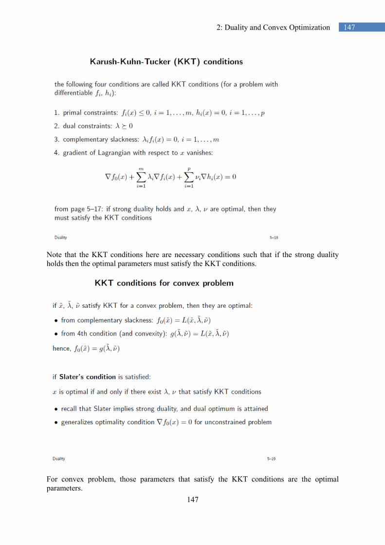
147
147 2: Duality and Convex Optimization
Note that the KKT conditions here are necessary conditions such that if the strong duality holds then the optimal parameters must satisfy the KKT conditions.
For convex problem, those parameters that satisfy the KKT conditions are the optimal parameters.

148 Chapter VII: Review of Mathematical Results

149
149 3: Some Useful Linear Algebra Results
3. Some Useful Linear Algebra Results A. Some Facts on the Matrix Norm Let us consider the following equalities:
Let A be an M K× matrix, M K≥ . Note the following equalites:
22
2 22 2
max22
0 0
max
max
max max
( the eigenvector for )
T T
T
Ax x A Ax
x xx x
x x
xxλ λ
λ
≠ ≠=
=
=
(177)
Let maxλ be the largest eigenvalue of the non-negative definite K K× matrix TA A .
The maximum gain
2
2max
0max
Ax
xxλ
≠= (178)
is called the matrix norm or spectral norm of A. Then, the matrix norm of TA A is maxλ .
Similarlry, let minλ be the minimum eigenvalue of the non-negative definite matrix. Then,
the minimum gain is
2
2min
0min
Ax
xxλ
≠= . (179)
B. Other useful matrix norm properties Suppose TA A= be K K× matrix. Then, TA U U= Σ is the eigenvalue decomposition where U is the unitary matrix, and the diagonal matrix Σ ’s entries are the sorted eigenvalues, such as 1 Kλ λ≥ ≥ . The following are true for any x:
1T Tx Ax x xλ≤
T TKx Ax x xλ≥
For any x, Ax A x≤ .
A B A B+ ≤ + (Triangle inequality)
0 0A A= ⇔ =

150 Chapter VII: Review of Mathematical Results
AB A B≤

151
151 3: Some Useful Linear Algebra Results
Chapter VIII. REFERENCES
[1] Claude E. Shannon, “Communication in the Presence of Noise,” Proceeding of the I.R.E., vol. 37, pp. 10-21, January, 1949.
[2] J. M. Whittaker, “Interpolatory Function Theory,” Cambridge Tracts in Mathematics and Mathematical Physics, No. 33, Cambridge University Press, Chapt. IV; 1935.
[3] David L. Donoho, “Compressed Sensing,” IEEE Trans. Information Theory, vol. 52, no. 4, pp. 12891306, Apr. 2006.
[4] David L. Donoho and Jared Tanner, “Precise Undersampling Theorems,” Proceedings of the IEEE, vol. 98, pp. 913-924, May, 2010.
[5] Richard Baraniuk, “Lecture Notes: Compressive Sensing,” IEEE Signal Processing Magazine, p. 118-121, July, 2007.
[6] Justin Romberg, “Imaging via compressive sampling,” IEEE Signal Processing Magazine, 25(2), pp. 14 - 20, March 2008.
[7] Ashikhmin, A. and Calderbank, A.R., “Grassmannian Packings from Operator Reed-Muller Codes,” IEEE Trans. Information Theory, vol. 56, Issue: 11, pp. 5689-5714, 2010.
[8] Emmanuel Candès and Terence Tao, Near optimal signal recovery from random projections: Universal encoding strategies? (IEEE Trans. on Information Theory, 52(12), pp. 5406 - 5425, December 2006)
[9] Emmanuel Candès and Terence Tao, “Decoding by linear programming,” IEEE Trans. on Information Theory, 51(12), pp. 4203 - 4215, December 2005.
[10] Emmanuel Candès, Justin Romberg, and Terence Tao, Robust uncertainty principles: Exact signal reconstruction from highly incomplete frequency information. (IEEE Trans. on Information Theory, 52(2) pp. 489 - 509, February 2006)
[11] Dimitri P. Bertsekas, A. Nedic and A.E. Ozdaglar, Convex Analysis and Optimization, Athena Scientific, 2003.
[12] S. Boyd and L. Vandenberghe, Convex Optimization, Cambridge University Press, 2004. D.
[13] Donoho and X. Huo, “Uncertainty Principles and Ideal Atomic Decomposition,” IEEE Trans. on Info. Theory, vol.47, no.7, Nov. 2001.
[14] M. Elad and A. Bruckstein, “A generalized uncertainty principle and sparse representation in pairs of bases,” IEEE Trans. Info. Theory, vol. 48, no. 9, Sept. 2002.
[15] J. Romberg, E. Candes, and T. Tao, “Robust Uncertainty Principles and Optimally Sparse Decompositions,” Presentation Downloaded from http://www.ipam.ucla.edu/publications/mgaws1/mgaws1_5184.pdf.
[16] Leon S. Lasdon, Optimization Theory for Large Systems, Dover publication, 2002. [17] Scott Shaobing Chen, David L. Donoho, and Michael A. Saunders, “Atomic
Decomposition by Basis Pursuit,” Vol. 43, no.1, pp. 129-159, SIAM Review, 2001. [18] D.L. Donoho and Y. Tsaig, “Fast Solution of l-1 Norm Minimization Problems
When the Solution May Be Sparse,” IEEE Transactions on Information Theory, vol. 54, no. 11, pp. 4789-4812, Nov. 2008.
[19] J. A. Tropp, “Greed is good: Algorithmic results for sparse approximation,” IEEE Trans. Inf. Theory, vol. 50, no. 10, pp. 2231–2242, Oct. 2004.
[20] J. A. Tropp, “Just relax: Convex programming methods for subset selection and sparse approximation,” IEEE Trans. Inf. Theory, vol. 51, no. 3, pp. 1030–1051, Mar.

152 Chapter VIII: References
2006. [21] M. R. Osborne, B. Presnell, and B. A. Turlach, “A new approach to variable
selection in least squares problems,” IMA J. Numer. Anal., vol. 20, pp. 389–403, 2000.
[22] M. R. Osborne, B. Presnell, and B. A. Turlach, “On the LASSO and its dual,” J. Comput. Graph. Stat., vol. 9, pp. 319–337, 2000.
[23] R. Tibshirani, “Regression shrinkage and selection via the lasso,” J. Roy. Statist. Soc., vol. 58, no. 1, pp. 267–288, 1996.
[24] D. L. Donoho, A. Maleki, and A. Montanari, “Message-passing algorithms for compressed sensing,” vol.106, no.45, Proceedings of National Academy of Science, Nov. 10, 2009.
[25] H. Rauhut, Theoretical Foundations and Numerical Methods for Sparse Recovery, volume 9 of Radon Series Comp. Appl. Math., pages 1-92. deGruyter, 2010. http://rauhut.ins.uni-bonn.de/research/pub.php?list=rauhut.
[26] Y.C. Chen, et. al, “Terahertz Pulsed Spectroscopic Imaging Using Optimized Binary Masks,” Applied Physics Letters 95, 231112, 2009.
[27] W.L. Chan, M.L. Moravec, R.G. Baraniuk, and D. Mittleman, “Terahertz imaging with compressed sensing and phase retrieval,” Optics Letters, vol. 33, no. 9, May 1, 2008.
[28] Michael Elad, Sparse and Redundant Representations: From theory to applications in signal processing and image processing, Springer Science, New York, 2010.
[29] D. L. Donoho, M. Elad, and V. Temlyakov. Stable recovery of sparse overcomplete representations in the presence of noise. submitted to IEEE Trans. Inform. Theory, February 2004.
[30] E. J. Candès, J. Romberg and T. Tao. Stable signal recovery from incomplete and
inaccurate measurements. Comm. Pure Appl. Math., 59 1207-1223.
[31] Lawson and Hanson, "Solving Least Squares Problems", Prentice-Hall, 1974,
Chapter 23, p. 161.
[32] Donoho and M. Elad, “Optimally Sparse Representation in General Dictionaries via
L1 Minimization, …
[33] E. J. Candes, “Compressed Sampling,” Proc. of the Int. Congress of
Mathematicians, Madrid, Spain, 2006.
[34] S.J. Park and Heung-No Lee, “On the Derivation of RIP for Random Gaussian
Matrices and Binary Sparse Signals,” Proc. of International Conference on ICT
Convergence 2011 (ICTC 2011), Seoul, Korea, Sept. 28-30, 2011.
[35] G. Tang and A. Nehorai, “Performance Analysis for Sparse Support Recovery,”
IEEE Trans. Info. Theory, vol. 56, no. 3, pp. 1383-1399, March, 2010.