Embed Size (px)
Citation preview
1.04.2017
1
Backpropagation
Networks
Introduction to
Backpropagation
- In 1986 a method for learning in multi-layer network,
Backpropagation, was invented by Rumelhart Paper Why are “what” and “where” processed by separate cortical visual systems?
- The Backpropagation algorithm is a sensible approach
for dividing the contribution of each weight.
- Works basically the same as perceptrons
Backpropagation Learning Principles:
Hidden Layers and Gradients
There are two differences for the updating rule :
1) The activation of the hidden unit is used instead of
activation of the input value.
2) The rule contains a term for the gradient of the activation
function.
Backpropagation Network
training
• 1. Initialize network with random weights
• 2. For all training cases (called examples):
– a. Present training inputs to network and calculate output
– b. For all layers (starting with output layer, back to input layer):
• i. Compare network output with correct output
(error function)
• ii. Adapt weights in current layer
This is
what
you
want
Backpropagation Learning
Details
• Method for learning weights in feed-forward (FF) nets
• Can’t use Perceptron Learning Rule – no teacher values are possible for hidden units
• Use gradient descent to minimize the error – propagate deltas to adjust for errors
backward from outputs
to hidden layers
to inputs forward
backward
Backpropagation Algorithm – Main Idea –
error in hidden layers
The ideas of the algorithm can be summarized as follows :
1. Computes the error term for the output units using the
observed error.
2. From output layer, repeat
- propagating the error term back to the previous layer
and
- updating the weights between the two layers
until the earliest hidden layer is reached.
1.04.2017
2
Backpropagation Algorithm
• Initialize weights (typically random!)
• Keep doing epochs
– For each example e in training set do
• forward pass to compute
– O = neural-net-output(network,e)
– miss = (T-O) at each output unit
• backward pass to calculate deltas to weights
• update all weights
– end
• until tuning set error stops improving
Backward pass explained in next slide Forward pass explained as a
perceptron earlier
Backward Pass
• Compute deltas to weights
– from hidden layer
– to output layer
• Without changing any weights (yet),
compute the actual contributions
– within the hidden layer(s)
– and compute deltas
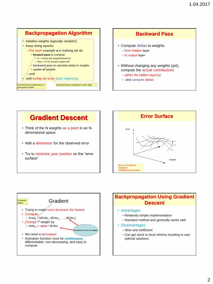
Gradient Descent
• Think of the N weights as a point in an N-
dimensional space
• Add a dimension for the observed error
• Try to minimize your position on the “error
surface”
Error Surface
Error as function of
weights in
multidimensional space
error
weights
Gradient
• Trying to make error decrease the fastest
• Compute: • GradE = [dE/dw1, dE/dw2, . . ., dE/dwn]
• Change ith weight by
• deltawi = -alpha * dE/dwi
• We need a derivative!
• Activation function must be continuous, differentiable, non-decreasing, and easy to compute
Derivatives of error for weights
Compute
deltas
Backpropagation Using Gradient
Descent
• Advantages
– Relatively simple implementation
– Standard method and generally works well
• Disadvantages
– Slow and inefficient
– Can get stuck in local minima resulting in sub-
optimal solutions
1.04.2017
3
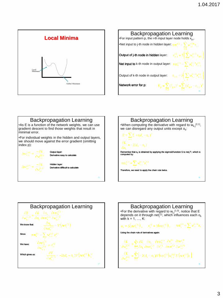
Local Minima
Local Minimum
Global Minimum
14
Backpropagation Learning •For input pattern p, the i-th input layer node holds xp,i.
•Net input to j-th node in hidden layer:
n
i
ipijj xwnet0
,
)0,1(
,
)1(
K
k
kpkp
K
k
kpp odlE1
2
,,
1
2
, )()(Network error for p:
j
jpjkkp xwSo )1(
,
)1,2(
,,Output of k-th node in output layer:
j
jpjkk xwnet )1(
,
)1,2(
,
)2(Net input to k-th node in output layer:
n
i
ipijjp xwSx0
,
)0,1(
,
)1(
,Output of j-th node in hidden layer:
15
Backpropagation Learning •As E is a function of the network weights, we can use gradient descent to find those weights that result in minimal error.
•For individual weights in the hidden and output layers, we should move against the error gradient (omitting index p):
)1,2(
,
)1,2(
,
jk
jkw
Ew
)0,1(
,
)0,1(
,
ij
ijw
Ew
Output layer:
Derivative easy to calculate
Hidden layer:
Derivative difficult to calculate
16
Backpropagation Learning •When computing the derivative with regard to wk,j
(2,1), we can disregard any output units except ok:
ki
kki odlE 22 )(
)(2 kk
k
odo
E
Remember that ok is obtained by applying the sigmoid function S to netk(2), which is
computed by:
j
jjkk xwnet )1()1,2(
,
)2(
Therefore, we need to apply the chain rule twice.
17
Backpropagation Learning
)1.2(
,
)2(
)2()1.2(
, jk
k
k
k
kjk w
net
net
o
o
E
w
E
Since
j
jjkk xwnet )1()1,2(
,
)2(
)1(
)1.2(
,
)2(
j
jk
k xw
net
We have:
We know that:
)2(
)2(' k
k
k netSnet
o
Which gives us:
)1()2(
)1.2(
,
')(2 jkkk
jk
xnetSodw
E
18
Backpropagation Learning •For the derivative with regard to wj,i
(1,0), notice that E depends on it through netj
(1), which influences each ok with k = 1, …, K:
Using the chain rule of derivatives again:
, )2(
kk netSo i
iijj xwnet )0,1(
,
)1( , )1()1(
jj netSx
)0,1(
,
)1(
)1(
)1(
1)1(
)2(
)2()0,1(
, ij
j
j
jK
k j
k
k
k
kij w
net
net
x
x
net
net
o
o
E
w
E
K
k
ijjkkkk
ij
xnetSwnetSodw
E
1
)1()1,2(
,
)2(
)0,1(
,
'')(2

1.04.2017
4
19
Backpropagation Learning
•This gives us the following weight changes at the output layer:
… and at the inner layer:
with)1()1.2(
, jkjk xw
)2(')( kkkk netSod
with)0,1(
, ijij xw
)1(
1
)1,2(
, ' j
K
k
jkkj netSw
20
Backpropagation Learning •As you surely remember from a few minutes ago:
Then we can simplify the generalized error terms:
))(1)(()(' xSxSxS
)2(')( kkkk netSod
)1()( kkkkk oood And:
)1(
1
)1,2(
, ' j
K
k
jkkj netSw
)1()1(
1
)1,2(
, 1 jj
K
k
jkkj xxw
22
Backpropagation Learning •The simplified error terms k and j use variables that are calculated in the feedforward phase of the network and can thus be calculated very efficiently.
•Now let us state the final equations again and reintroduce the subscript p for the p-th pattern:
with)1(
,,
)1.2(
, jpkpjk xw
)1()( ,,,,, kpkpkpkpkp oood
with,,
)0,1(
, ipjpij xw
)1(
,
)1(
,
1
)1,2(
,,, 1 jpjp
K
k
jkkpjp xxw
How do we pick ?
1. Tuning set, or
2. Cross validation, or
3. Small for slow, conservative learning
How many hidden layers?
• Usually just one (i.e., a 2-layer net)
• How many hidden units in the layer?
– Too few ==> can’t learn
– Too many ==> poor generalization
1.04.2017
5
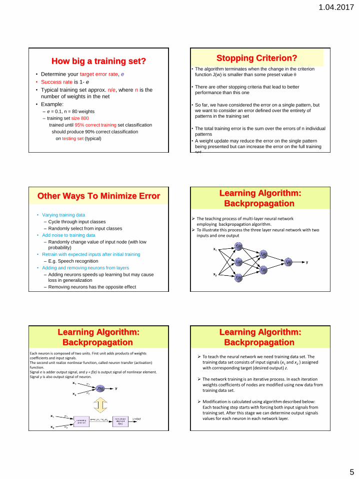
How big a training set?
• Determine your target error rate, e
• Success rate is 1- e
• Typical training set approx. n/e, where n is the
number of weights in the net
• Example:
– e = 0.1, n = 80 weights
– training set size 800
trained until 95% correct training set classification
should produce 90% correct classification
on testing set (typical)
• The algorithm terminates when the change in the criterion
function J(w) is smaller than some preset value
• There are other stopping criteria that lead to better
performance than this one
• So far, we have considered the error on a single pattern, but
we want to consider an error defined over the entirety of
patterns in the training set
• The total training error is the sum over the errors of n individual
patterns
• A weight update may reduce the error on the single pattern
being presented but can increase the error on the full training
set
Stopping Criterion?
Other Ways To Minimize Error
• Varying training data
– Cycle through input classes
– Randomly select from input classes
• Add noise to training data
– Randomly change value of input node (with low
probability)
• Retrain with expected inputs after initial training
– E.g. Speech recognition
• Adding and removing neurons from layers
– Adding neurons speeds up learning but may cause
loss in generalization
– Removing neurons has the opposite effect
Learning Algorithm:
Backpropagation
The teaching process of multi-layer neural network employing backpropagation algorithm.
To illustrate this process the three layer neural network with two inputs and one output
Each neuron is composed of two units. First unit adds products of weights coefficients and input signals. The second unit realize nonlinear function, called neuron transfer (activation) function. Signal e is adder output signal, and y = f(e) is output signal of nonlinear element. Signal y is also output signal of neuron.
Learning Algorithm:
Backpropagation
To teach the neural network we need training data set. The training data set consists of input signals (x1 and x2 ) assigned with corresponding target (desired output) z.
The network training is an iterative process. In each iteration weights coefficients of nodes are modified using new data from training data set.
Modification is calculated using algorithm described below: Each teaching step starts with forcing both input signals from training set. After this stage we can determine output signals values for each neuron in each network layer.
Learning Algorithm:
Backpropagation
1.04.2017
6
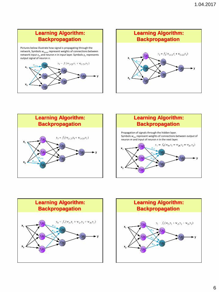
Pictures below illustrate how signal is propagating through the network, Symbols w(xm)n represent weights of connections between network input xm and neuron n in input layer. Symbols yn represents output signal of neuron n.
Learning Algorithm:
Backpropagation
Learning Algorithm:
Backpropagation
Learning Algorithm:
Backpropagation
Propagation of signals through the hidden layer. Symbols wmn represent weights of connections between output of neuron m and input of neuron n in the next layer.
Learning Algorithm:
Backpropagation
Learning Algorithm:
Backpropagation
Learning Algorithm:
Backpropagation
1.04.2017
7
Propagation of signals through the output layer.
Learning Algorithm:
Backpropagation
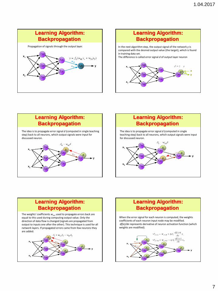
In the next algorithm step, the output signal of the network y is compared with the desired output value (the target), which is found in training data set. The difference is called error signal d of output layer neuron
Learning Algorithm:
Backpropagation
The idea is to propagate error signal d (computed in single teaching step) back to all neurons, which output signals were input for discussed neuron.
Learning Algorithm:
Backpropagation
The idea is to propagate error signal d (computed in single teaching step) back to all neurons, which output signals were input for discussed neuron.
Learning Algorithm:
Backpropagation
The weights' coefficients wmn used to propagate errors back are equal to this used during computing output value. Only the direction of data flow is changed (signals are propagated from output to inputs one after the other). This technique is used for all network layers. If propagated errors came from few neurons they are added.
Learning Algorithm:
Backpropagation
When the error signal for each neuron is computed, the weights coefficients of each neuron input node may be modified. df(e)/de represents derivative of neuron activation function (which weights are modified).
Learning Algorithm:
Backpropagation
1.04.2017
8
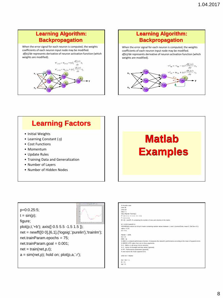
When the error signal for each neuron is computed, the weights coefficients of each neuron input node may be modified. df(e)/de represents derivative of neuron activation function (which weights are modified).
Learning Algorithm:
Backpropagation
When the error signal for each neuron is computed, the weights coefficients of each neuron input node may be modified. df(e)/de represents derivative of neuron activation function (which weights are modified).
Learning Algorithm:
Backpropagation
Learning Factors
• Initial Weights
• Learning Constant ()
• Cost Functions
• Momentum
• Update Rules
• Training Data and Generalization
• Number of Layers
• Number of Hidden Nodes
Matlab
Examples
p=0:0.25:5;
t = sin(p);
figure;
plot(p,t,'+b'); axis([-0.5 5.5 -1.5 1.5 ]);
net = newff([0 0],[6,1],{'logsig','purelin'},'trainlm');
net.trainParam.epochs = 75;
net.trainParam.goal = 0.001;
net = train(net,p,t);
a = sim(net,p); hold on; plot(p,a,'.r');
% bi-polar case
clear all
close all
disp (' ');
disp ('Bipolar Training');
P = [1 1 1 1; -1 -1 1 1; -1 1 -1 1]
T = [-1 1 1 1]
[R, Q] = size(P); % containing the number of rows and columns in the matrix.
W = 0.001*randn(R,1);
%RANDN(N) returns an N-by-N matrix containing random values between -1 and 1 (normal Distn, mean 0, Std Dev of 1)
alpha = 0.15;
err = 0.1;
MaxIter = 1000;
iter = 0;
MSE = [];
% MSE is a network performance function. It measures the network's performance according to the mean of squared errors.
% MSE(E,X,PP) takes from one to three arguments,
% E - Matrix or cell array of error vector(s).
% X - Vector of all weight and bias values (ignored).
% PP - Performance parameters (ignored).
% and returns the mean squared error.
while iter < MaxIter
iter = iter + 1;
Er = 0;
tqe = 0;

1.04.2017
9
for k = 1:Q %q pattern, each training case, 4 cases in total, no of columns in P
v = P(:, k)'*W; % v = w'(x) x(k); w= 3x1 matrix; x = 3x1 matrix; w'x = 1x1
e = T(k) - v; %desired value - v
n2 = norm (P(:, k)); % NORM(V,P) = sum(abs(V).^P)^(1/P). NORM(V) = norm(V,2).
if n2~=0
W = W + alpha * e * P(:,k) / n2 ^ 2; %change weight
end
Er = Er + 1/Q*e^2;
end
MSE = [MSE Er];
if Er <= err
fprintf(1, 'err satisfied \n');
break;
end
span = 10;
if iter > (span+1)
de = MSE(iter) - MSE(iter - span);
if abs(de) < 1e-7
fprintf(1, 'the network is updating too slow\n');
break
end
end
end
W
iter
% the rest of the program
figure;
plot(MSE);
title('Bipolar Training MSE performance');
xlabel('Epochs');
ylabel('MSE');
rng default; % For reproducibility %random kmeans
X = [randn(100,2)*0.75+ones(100,2);
randn(100,2)*0.5-ones(100,2)];
figure;
plot(X(:,1),X(:,2),'.');
title 'Randomly Generated Data';
opts = statset('Display','final');
[idx,C] = kmeans(X,2,'Distance','cityblock',...
'Replicates',5,'Options',opts);
figure;
plot(X(idx==1,1),X(idx==1,2),'r.','MarkerSize',12)
hold on
plot(X(idx==2,1),X(idx==2,2),'b.','MarkerSize',12)
plot(C(:,1),C(:,2),'kx',...
'MarkerSize',15,'LineWidth',3)
legend('Cluster 1','Cluster 2','Centroids',...
'Location','NW')
title 'Cluster Assignments and Centroids'
hold off