Introduction to Fuzzy Control

Hans P. Geering

Abstract

In this report, some of the basic mathematical definitions and rulesof fuzzy system theory are described inasmuch as they are relevant forfuzzy control. Two examples are covered in detail, viz., a fuzzy closed-loop halting control scheme for the forward motion of a mobile robot inan automatic factory and a dog chasing a cat using fuzzy control.

Issues of computational efficiency are discussed. And some recommen-dations to potential designers of fuzzy controllers are summarized.

After studying this report, the reader should be in a position to designsimple fuzzy controllers and simulate the behaviour of the resulting fuzzycontrol system on a general purpose digital computer.

IMRT Press

c© Measurement and Control LaboratorySwiss Federal Institute of Technology (ETH)

ETH-ZentrumCH-8092 Zurich, Switzerland

3rd ed., September, 1998

ii GEERING: FUZZY CONTROL

CONTENTS iii

Contents

1 Fuzzy Sets . . . . . . . . . . . . . . . . . . . . . . . . . . . . . . . . 1

2 Fuzzification . . . . . . . . . . . . . . . . . . . . . . . . . . . . . . . 2

3 Fuzzy Logic . . . . . . . . . . . . . . . . . . . . . . . . . . . . . . . 2

4 Fuzzy Variables . . . . . . . . . . . . . . . . . . . . . . . . . . . . 34.1 Introducing Fuzzy Variables . . . . . . . . . . . . . . . . . . . . . 34.2 Fuzziflcation Revised . . . . . . . . . . . . . . . . . . . . . . . . . 44.3 Fuzzy Vectors . . . . . . . . . . . . . . . . . . . . . . . . . . . . . 4

5 Fuzzy Rules . . . . . . . . . . . . . . . . . . . . . . . . . . . . . . . 55.1 Fuzzy SISO-Rule . . . . . . . . . . . . . . . . . . . . . . . . . . . 55.2 Fuzzy AND-Rules . . . . . . . . . . . . . . . . . . . . . . . . . . 55.3 Other Fuzzy Rules . . . . . . . . . . . . . . . . . . . . . . . . . . 6

6 Fuzzy Associative Memory . . . . . . . . . . . . . . . . . . . . . 6

7 Defuzzification . . . . . . . . . . . . . . . . . . . . . . . . . . . . . 7

8 Fuzzy Control Systems . . . . . . . . . . . . . . . . . . . . . . . . 88.1 Structure of a Fuzzy Control System . . . . . . . . . . . . . . . . 88.2 Example 1: Closed-loop halting control . . . . . . . . . . . . . . 108.3 Example 2: Dog chasing cat . . . . . . . . . . . . . . . . . . . . . 15

9 Computational Issues . . . . . . . . . . . . . . . . . . . . . . . . . 189.1 E–cient Defuzziflcation . . . . . . . . . . . . . . . . . . . . . . . 189.2 Derivatives of the Control Function . . . . . . . . . . . . . . . . . 209.3 Observations and Suggestions . . . . . . . . . . . . . . . . . . . . 21

References . . . . . . . . . . . . . . . . . . . . . . . . . . . . . . . . . . 22

iv GEERING: FUZZY CONTROL

1 FUZZY SETS 1

1 Fuzzy Sets

Definition: A fuzzy set s is an ordered pair (X, f), where X is a vector space(usually the real line R) and f is a set membership function mapping X ontothe interval [0, 1] of the real line R, i.e., f : X → [0, 1].

In a fuzzy control problem, X is the signal space of a signal or a vectorsignal, respectively.

A set S ⊂ X is associated with the fuzzy set s = (X, f) in a natural way:S = cl{x∈X | f(x)> 0} is the closure of the set in X where f attains positivevalues.

Notice that the set membership function f is normalized in the sense thatthe value f(x) = 1 is attained for at least one element x ∈ S ⊂ X. However, thisnormalization has mainly been introduced for practical and intuitive reasons.Mathematically speaking, this normalization is dispensable.

Usually, a fuzzy set is a constant construct, i.e., a time-invariant part of afuzzy control system.

-

6

1

0-20 -10 0 10 20

fi

X�����AAAAA

Z

����� T

TTTT

PS

�����

PL

����� T

TTTT

NS

@@@@@

NL

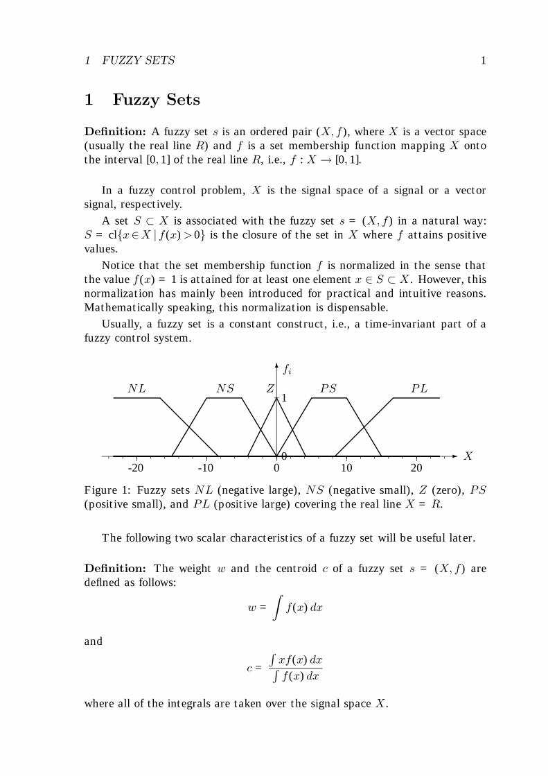
Figure 1: Fuzzy sets NL (negative large), NS (negative small), Z (zero), PS(positive small), and PL (positive large) covering the real line X = R.

The following two scalar characteristics of a fuzzy set will be useful later.

Definition: The weight w and the centroid c of a fuzzy set s = (X, f) aredeflned as follows:

w =∫f(x) dx

and

c =∫xf(x) dx∫f(x) dx

where all of the integrals are taken over the signal space X.

2 GEERING: FUZZY CONTROL

2 Fuzzification

Consider a signal space X covered by several fuzzy sets si, i = 1, . . . , k. Thefuzzy question is: Given a vector x ∈ X, to which of the fuzzy sets si does xbelong or, in which of the sets Si associated with the fuzzy sets si does x lie?

In mathematical set theory, the answer for each of the sets Si is a binaryone. In fuzzy set theory, set membership is \by degree".

Definition: Consider a fuzzy set s = (X, f). An arbitrary element x ∈ Xbelongs to the fuzzy set s with degree d = f(x).

Hence, the answer to the fuzzy question is: x belongs to each of the fuzzysets si to some degree, viz., to degrees di = fi(x), i = 1, . . . , k.

Examples: Consider the fuzzy sets NL, NS, Z, PS, and PL deflned on thesignal space X = R which are displayed in Figure 1.

a) The element x = −20 is \negative large" to degree 1 and \negative small",\zero", \positive small", and \positive large" to degrees 0.

b) The element x = 2 is \negative large" and \negative small" to degrees 0,\zero" to degree 0.52, \positive small" to degree 0.4, and \positive large" todegree 0.

3 Fuzzy Logic

Fuzzy logic deflnes the rules governing the operators intersection and union offuzzy sets.

Consider two fuzzy sets s1 = (X, f1) and s2 = (X, f2) deflned on the samesignal space X and their associated sets S1 ⊂ X and S2 ⊂ X, respectively.

Definition: An arbitrary element x ∈ X belongs to the union s1 ∪ s2 of thetwo fuzzy sets s1 and s2 with degree d = max(f1(x), f2(x)).

Definition: An arbitrary element x ∈ X belongs to the intersection s1 ∩ s2 ofthe two fuzzy sets s1 and s2 with degree d = min(f1(x), f2(x)).

Consequently, the union operator and the intersection operator yield thefuzzy sets s1∪s2 = (X,max(f1, f2)) and s1∩s2 = (X,min(f1, f2)), respectively.Notice that the intersection s1 ∩ s2 is a degenerated fuzzy set in the sense thatits set membership function min(f1, f2) does not map onto the interval [0, 1] asrequested by the deflnition of a fuzzy set. This detail is not pursued any furtherhere because in fuzzy control, all calculations are done with fuzzy variablesrather than with fuzzy sets.

4 FUZZY VARIABLES 3

4 Fuzzy Variables

4.1 Introducing Fuzzy Variables

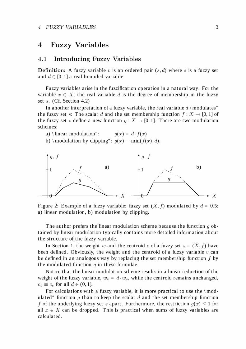
Definition: A fuzzy variable v is an ordered pair (s, d) where s is a fuzzy setand d ∈ [0, 1] a real bounded variable.

Fuzzy variables arise in the fuzziflcation operation in a natural way: For thevariable x ∈ X, the real variable d is the degree of membership in the fuzzyset s. (Cf. Section 4.2)

In another interpretation of a fuzzy variable, the real variable d \modulates"the fuzzy set s: The scalar d and the set membership function f : X → [0, 1] ofthe fuzzy set s deflne a new function g : X → [0, 1]. There are two modulationschemes:

a) \linear modulation": g(x) = d ·f(x)b) \modulation by clipping": g(x) = min(f(x), d).

- -

6 6

1 1

0 0

g, f g, f

X X

f f

g g

a) b)

p p p p p p pp p pp p p p p pp p p p p p p p p p p pp p p p p p p p p p p p p p p p p p p p p p

p p pp p p p p pp p p p p p p p p p p pp p p p p p p p p p p p p p p��

��XXXHHHH �

��� @

@@

Figure 2: Example of a fuzzy variable: fuzzy set (X, f) modulated by d = 0.5:a) linear modulation, b) modulation by clipping.

The author prefers the linear modulation scheme because the function g ob-tained by linear modulation typically contains more detailed information aboutthe structure of the fuzzy variable.

In Section 1, the weight w and the centroid c of a fuzzy set s = (X, f) havebeen deflned. Obviously, the weight and the centroid of a fuzzy variable v canbe deflned in an analogous way by replacing the set membership function f bythe modulated function g in these formulae.

Notice that the linear modulation scheme results in a linear reduction of theweight of the fuzzy variable, wv = d ·ws, while the centroid remains unchanged,cv ≡ cs for all d ∈ (0, 1].

For calculations with a fuzzy variable, it is more practical to use the \mod-ulated" function g than to keep the scalar d and the set membership functionf of the underlying fuzzy set s apart. Furthermore, the restriction g(x) ≤ 1 forall x ∈ X can be dropped. This is practical when sums of fuzzy variables arecalculated.

4 GEERING: FUZZY CONTROL

4.2 Fuzzification Revised

Consider a signal space X covered by the N fuzzy sets s1, . . . , sN . An arbitraryelement x ∈ X belongs to the fuzzy sets s1, s2, . . . , and sN to degrees d1 = f1(x),d2 = f2(x), . . . , and dN = fN (x), respectively.

Using fuzzy variables leads to the following deflnition of the fuzziflcationoperation.

Definition: The fuzziflcation operator F maps an element x ∈ X to the set offuzzy variables {(s1, f1(x)), (s2, f2(x)), . . . (sN , fN (x))}.

Examples: Reconsider the examples a) and b) of Section 2. With the abovedeflnition we can rewrite the results succinctly in the following way:

a) F : −20 7→ {(NL, 1), (NS, 0), (Z, 0), (PS, 0), (PL, 0)} andb) F : 2 7→ {(NL, 0), (NS, 0), (Z, 0.52), (PS, 0.4), (PL, 0)}.

4.3 Fuzzy Vectors

As the example in Section 4.2 shows, introducing vector notation in the rangespace of the fuzziflcation operator F is e–cient.

Again, consider a signal space X covered by the N fuzzy sets s1, . . . , sN .The fuzziflcation F(x) of an arbitrary element x ∈ X can be represented by anN -vector in several equivalent ways:

F(x) =

v1

v2...vN

(x) =

(s1, f1(x))(s2, f2(x))

...(sN , fN (x))

∼=f1(x)f2(x)

...fN (x)

.

The relation operator \∼=" points out the fact that, in the last vector, the fuzzysets si are not explicitly noted down but are implied by the indices i.

On the other side, every fuzzy n-vector can be represented by the corre-sponding modulated set membership functions gi:

v1

v2...vn

=

(s1, d1)(s2, d2)

...(sn, dn)

=

g1

g2...gn

∼=

(wg1 , cg1)(wg2 , cg2)

...(wgn , cgn)

.

Here, the relation operator \∼=" points out the fact that the weight wgi andthe centroid cgi do not completely characterize the fuzzy variable vi.

This representation is useful at the outputs of the fuzzy rules describing afuzzy controller.

5 FUZZY RULES 5

5 Fuzzy Rules

Fuzzy rules are used in fuzzy control in order to deflne the map from the fuzzifledinput signals (error signals, measured signals, or command signals) of the fuzzycontroller to its fuzzy output signals (control signals).

5.1 Fuzzy SISO-Rule

Consider a fuzzy set se = (E, fe) deflned on the signal space E where the errorsignal e \lives" and a fuzzy set su = (U, fu) deflned on the signal space U wherethe control signal u \lives". (Usually, E = R and U = R, hence the designation\SISO-rule".)

Definition: The SISO-rule mapping the fuzzy input variable ve = (se, de) tothe fuzzy output variable vu = (su, du) (of the fuzzy controller) is deflned byvu = (su, de).

In the jargon of control engineering, this deflnition should be read as follows:If the value e(t) of the error signal belongs to the fuzzy set se to degree de thenthe fuzzy set su of the control signal is flred to degree du = de, i.e., modulatedby du = de.

In shorthand notation, the fuzzy SISO-rule is denoted by se ⇒ su, wherethe degree of flring du = de is implied.

The value u(t) of the control signal is obtained later by \defuzziflcation"after all of the fuzzy rules pertaining to the control signal have been processed.

5.2 Fuzzy AND-Rules

Consider two fuzzy sets se1 = (E1, fe1) and se2 = (E2, fe2) deflned on the signalspaces E1 and E2, respectively, where the error signals e1 and e2 \live" and afuzzy set su = (U, fu) deflned on the signal space U where the control signal u\lives".

Definition: The AND-rule mapping the fuzzy input variables ve1 = (se1, de1)and ve2 = (se2, de2) to the fuzzy output variable vu = (su, du) is deflned byvu = (su,min(de1, de2)).

In the jargon of control engineering, this deflnition should be read as follows:If the value e1(t) of the flrst error signal belongs to the fuzzy set se1 to degreede1 and the value e2(t) of the second error signal belongs to the fuzzy set se2 todegree de2 then the fuzzy set su of the control signal is flred to the smaller ofthe two degrees, i.e., du = min(de1, de2).

In shorthand notation, the fuzzy AND-rule is denoted by se1 ∩ se2 ⇒ su,where the degree of flring du = min(de1 , de2) is implied.

6 GEERING: FUZZY CONTROL

The value u(t) of the control signal is obtained later by \defuzziflcation"after all of the fuzzy rules pertaining to the control signal have been processed.

It should be obvious how the deflnition of the fuzzy AND-rule can be ex-tended to three or more fuzzy input variables.

5.3 Other Fuzzy Rules

In analogy to the fuzzy AND-rules, fuzzy OR-rules or more complicated logicalcombinations for fuzzy rules could be deflned.

The author prefers to use fuzzy AND-rules exclusively because OR-ing sev-eral AND-rules together typically results in a weaker contribution to the overallfuzzy output variable(s) and the corresponding defuzzifled control variable(s).

Therefore, in the remainder of this report \fuzzy rule" stands for \fuzzyAND-rule" or its SISO special case \fuzzy SISO-rule".

6 Fuzzy Associative Memory

For a fuzzy controller, the collection of all of its fuzzy rules is called the fuzzyassociative memory.

For every control cycle, each of the fuzzy rules is evaluated. This can bedone by massively parallel processing. The output of each fuzzy rule is a fuzzyvariable.

The output of the fuzzy associative memory is equal to the (vector) sum ofall these fuzzy variables:

In the case of a scalar control signal u(t), the signal space is the real line,U = R. Summing the fuzzy variables involves calculating the sum gu =

∑j gj of

their modulated functions gj . | Notice that the fuzzy variable vu at the outputof the fuzzy associative memory is represented exclusively by the (\modulated")function gu. (I.e., this fuzzy variable has no directly underlying fuzzy set whichis modulated by some degree du to yield the function gu.)

In the case of a vector control signal u(t) ∈ Rm, typically, the signal spaceof each of the components ui(t) is the real line, i.e., Ui = R for i = 1, . . . ,m.Summing the fuzzy variables involves calculating the m sums gui =

∑j gij of

the modulated functions gij for each index i, i = 1, . . . ,m.Of course, the summing operator

∑takes the pointwise sum of its argument

functions. As mentioned in Section 4.1, the sum g(u) may execeed 1 for somevalues of the argument u. This poses no problem (cf. Section 7). (Clipping g(u)to the maximal value 1 would be counterproductive because the centroid of gwould be shifted.)

7 DEFUZZIFICATION 7

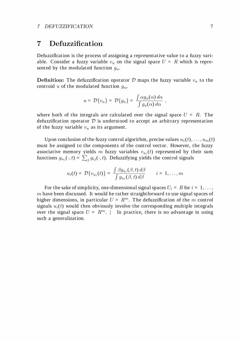
7 Defuzzification

Defuzziflcation is the process of assigning a representative value to a fuzzy vari-able. Consider a fuzzy variable vu on the signal space U = R which is repre-sented by the modulated function gu.

Definition: The defuzziflcation operator D maps the fuzzy variable vu to thecentroid u of the modulated function gu,

u = D{vu} = D{gu} =∫αgu(α) dα∫gu(α) dα

,

where both of the integrals are calculated over the signal space U = R. Thedefuzziflcation operator D is understood to accept an arbitrary representationof the fuzzy variable vu as its argument.

Upon conclusion of the fuzzy control algorithm, precise values u1(t), . . . , um(t)must be assigned to the components of the control vector. However, the fuzzyassociative memory yields m fuzzy variables vui(t) represented by their sumfunctions gui(·, t) =

∑j gij(·, t). Defuzzifying yields the control signals

ui(t) = D{vui(t)} =∫βgui(β, t) dβ∫gui(β, t) dβ

i = 1, . . . ,m

For the sake of simplicity, one-dimensional signal spaces Ui = R for i = 1, . . . ,m have been discussed. It would be rather straightforward to use signal spaces ofhigher dimensions, in particular U = Rm. The defuzziflcation of the m controlsignals ui(t) would then obviously involve the corresponding multiple integralsover the signal space U = Rm. | In practice, there is no advantage in usingsuch a generalization.

8 GEERING: FUZZY CONTROL

8 Fuzzy Control Systems

8.1 Structure of a Fuzzy Control System

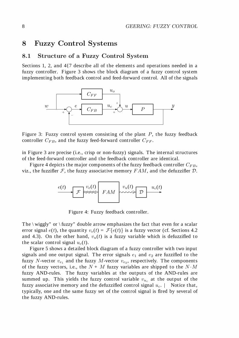
Sections 1, 2, and 4{7 describe all of the elements and operations needed in afuzzy controller. Figure 3 shows the block diagram of a fuzzy control systemimplementing both feedback control and feed-forward control. All of the signals

- i - CFB - i - P -

6

CFF-

?w yue uc

uo

+−

+

+

Figure 3: Fuzzy control system consisting of the plant P , the fuzzy feedbackcontroller CFB , and the fuzzy feed-forward controller CFF .

in Figure 3 are precise (i.e., crisp or non-fuzzy) signals. The internal structuresof the feed-forward controller and the feedback controller are identical.

Figure 4 depicts the major components of the fuzzy feedback controller CFB ,viz., the fuzzifler F , the fuzzy associative memory FAM , and the defuzzifler D.

- F ≈≈≈≈> FAM ∼∼∼∼∼> D -e(t) ve(t) vu(t) uc(t)

Figure 4: Fuzzy feedback controller.

The \wiggly" or \fuzzy" double arrow emphasizes the fact that even for a scalarerror signal e(t), the quantity ve(t) = F{e(t)} is a fuzzy vector (cf. Sections 4.2and 4.3). On the other hand, vu(t) is a fuzzy variable which is defuzzifled tothe scalar control signal uc(t).

Figure 5 shows a detailed block diagram of a fuzzy controller with two inputsignals and one output signal. The error signals e1 and e2 are fuzzifled to thefuzzy N -vector ve1 and the fuzzy M -vector ve2 , respectively. The componentsof the fuzzy vectors, i.e., the N + M fuzzy variables are shipped to the N ·Mfuzzy AND-rules. The fuzzy variables at the outputs of the AND-rules aresummed up. This yields the fuzzy control variable vuc at the output of thefuzzy associative memory and the defuzzifled control signal uc. | Notice that,typically, one and the same fuzzy set of the control signal is flred by several ofthe fuzzy AND-rules.

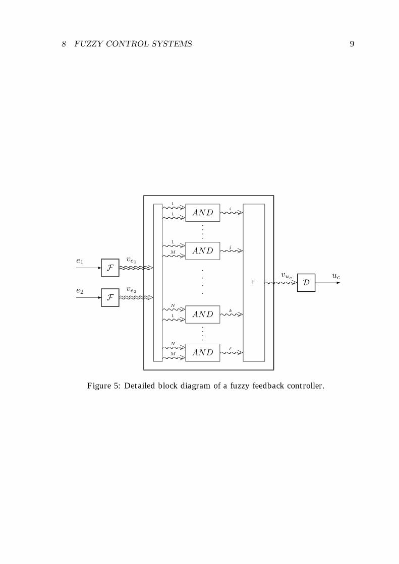
8 FUZZY CONTROL SYSTEMS 9

- F ≈≈≈≈≈≈>

- F ≈≈≈≈≈≈>e1 ve1

e2 ve2

∼∼∼∼>∼∼∼∼> ∼∼∼∼>AND

∼∼∼∼>∼∼∼∼> ∼∼∼∼>AND

pppp

∼∼∼∼>∼∼∼∼> ∼∼∼∼>AND

∼∼∼∼>∼∼∼∼> ∼∼∼∼>AND

pppp

pppp

+ ∼∼∼∼∼∼> D -vuc uc

1

1

1

M

N

1

N

M

i

j

k

`

Figure 5: Detailed block diagram of a fuzzy feedback controller.

10 GEERING: FUZZY CONTROL

8.2 Example 1: Closed-loop halting control

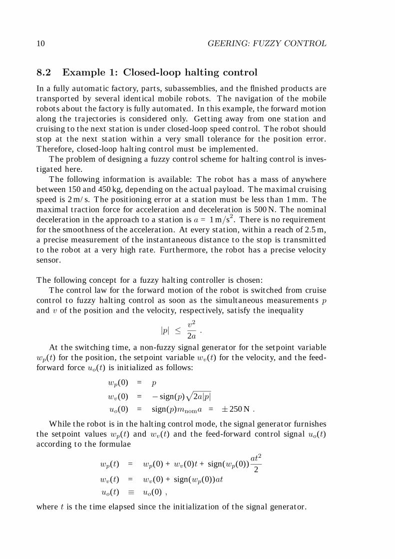
In a fully automatic factory, parts, subassemblies, and the flnished products aretransported by several identical mobile robots. The navigation of the mobilerobots about the factory is fully automated. In this example, the forward motionalong the trajectories is considered only. Getting away from one station andcruising to the next station is under closed-loop speed control. The robot shouldstop at the next station within a very small tolerance for the position error.Therefore, closed-loop halting control must be implemented.

The problem of designing a fuzzy control scheme for halting control is inves-tigated here.

The following information is available: The robot has a mass of anywherebetween 150 and 450 kg, depending on the actual payload. The maximal cruisingspeed is 2 m/s. The positioning error at a station must be less than 1 mm. Themaximal traction force for acceleration and deceleration is 500 N. The nominaldeceleration in the approach to a station is a = 1 m/s2. There is no requirementfor the smoothness of the acceleration. At every station, within a reach of 2.5 m,a precise measurement of the instantaneous distance to the stop is transmittedto the robot at a very high rate. Furthermore, the robot has a precise velocitysensor.

The following concept for a fuzzy halting controller is chosen:The control law for the forward motion of the robot is switched from cruise

control to fuzzy halting control as soon as the simultaneous measurements pand v of the position and the velocity, respectively, satisfy the inequality

|p| ≤ v2

2a.

At the switching time, a non-fuzzy signal generator for the setpoint variablewp(t) for the position, the setpoint variable wv(t) for the velocity, and the feed-forward force uo(t) is initialized as follows:

wp(0) = p

wv(0) = − sign(p)√

2a|p|uo(0) = sign(p)mnoma = ± 250 N .

While the robot is in the halting control mode, the signal generator furnishesthe setpoint values wp(t) and wv(t) and the feed-forward control signal uo(t)according to the formulae

wp(t) = wp(0) + wv(0)t+ sign(wp(0))at2

2wv(t) = wv(0) + sign(wp(0))atuo(t) ≡ uo(0) ,

where t is the time elapsed since the initialization of the signal generator.

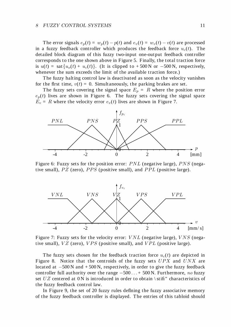
8 FUZZY CONTROL SYSTEMS 11

The error signals ep(t) = wp(t)− p(t) and ev(t) = wv(t)− v(t) are processedin a fuzzy feedback controller which produces the feedback force uc(t). Thedetailed block diagram of this fuzzy two-input one-output feedback controllercorresponds to the one shown above in Figure 5. Finally, the total traction forceis u(t) = sat{uo(t) + uc(t)}. (It is clipped to +500 N or −500 N, respectively,whenever the sum exceeds the limit of the available traction force.)

The fuzzy halting control law is deactivated as soon as the velocity vanishesfor the flrst time, v(t) = 0. Simultaneously, the parking brakes are set.

The fuzzy sets covering the signal space Ep = R where the position errorep(t) lives are shown in Figure 6. The fuzzy sets covering the signal spaceEv = R where the velocity error ev(t) lives are shown in Figure 7.

-

6

1

0-4 -2 0 2 4 [mm]

fpi

p�����AAAAA

PZ

�����@@@@@

PPS

����

����

��PPL

�����@@@@@

PNSHHHHHHHHHH

PNL

Figure 6: Fuzzy sets for the position error: PNL (negative large), PNS (nega-tive small), PZ (zero), PPS (positive small), and PPL (positive large).

-

6

1

0-4 -2 0 2 4 [mm/s]

fvi

v�����@@@@@

V Z

�����@@@@@

V PS

�����

V PL

�����@@@@@

V NS

@@@@@

V NL

Figure 7: Fuzzy sets for the velocity error: V NL (negative large), V NS (nega-tive small), V Z (zero), V PS (positive small), and V PL (positive large).

The fuzzy sets chosen for the feedback traction force uc(t) are depicted inFigure 8. Notice that the centroids of the fuzzy sets UPX and UNX arelocated at −500 N and +500 N, respectively, in order to give the fuzzy feedbackcontroller full authority over the range −500 . . .+ 500 N. Furthermore, no fuzzyset UZ centered at 0 N is introduced in order to obtain \stifi" characteristics ofthe fuzzy feedback control law.

In Figure 9, the set of 20 fuzzy rules deflning the fuzzy associative memoryof the fuzzy feedback controller is displayed. The entries of this tabloid should

12 GEERING: FUZZY CONTROL

-

6

1

0-500 0 500 [N]

fui

u������LLLLLL

UPS

�����TTTTT

UPL

����� T

TTTT

UPX

����� T

TTTT

UNX

�����TTTTT

UNL

������LLLLLL

UNS

Figure 8: Fuzzy sets for the control of the traction force: UNX (negative extralarge), UNL (negative large), UNS (negative small), UPS (positive small),UPL (positive large), and UPX (positive extra large).

be read as explained in the following example. Shorthand explanation: PNL∩V NL⇒ UNX. Longhand explanation: If ep(t) belongs to the fuzzy set PNL todegree d1 and if ev(t) belongs to the fuzzy set V NL to degree d2 then the fuzzyset UNX is flred to the smaller of the two degrees, i.e., to degree d = min(d1, d2).

PNL PNS PZ PPS PPL

vp : position error

V NL

V NS

V Z

V PS

V PL

vv :velocity

error

UNX

UNX UNX

UNL

UNL

UNL

UNS

UNS

UNS

UNS

UPS

UPS

UPS

UPS

UPL

UPL

UPL

UPX UPX

UPX

Figure 9: Fuzzy associative memory for the fuzzy closed-loop servo controllercontaining twenty fuzzy rules.

8 FUZZY CONTROL SYSTEMS 13

In order to evaluate the efiectiveness of the proposed fuzzy control scheme,the mobile robot is simulated. For the simulation, the \true" robot is modelledas follows:

_p(t) = v(t)p(0) = −2 m

_v(t) =1m{u(t)− sign(v(t))γmg}

v(0) = 2 m/s ,

where m = 150 . . . 450 kg is the true mass of the robot, g = 9.81 m/s2 thegravitational constant, and γ = 0.01 the coe–cient of roll friction. For thesimulations, digital control with a sampling and control rate of 500 Hz is as-sumed. This fairly high sampling rate is chosen in order to prevent mechanicalresonances in the mobile robot.

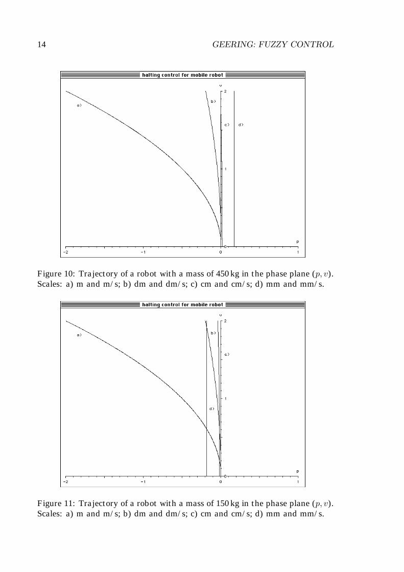
In Figures 10 and 11, the trajectory of the robot is shown in the phase plane(p, v) in several scales for a true mass m = 450 kg and m = 150 kg, respectively.For the complete trajectory labelled \a)", the units for p and v are m and m/s,respectively. For the increasingly enlarged flnal parts \b)", \c)", and \d)" ofthe trajectory, the units are dm and dm/s, cm and cm/s, and mm and mm/s,respectively.

As the Figures show, the heaviest robot (m = 450 kg) overshoots the stationby less than 0.2 mm, whereas the lightest robot (m = 150 kg) stops less than0.2 mm short of the station. Hence, the speciflcations are met.

This servo control example is deceptively simple because the plant under con-sideration essentially is a double integrator and because with a PD-controlleror with the equivalent linear state feedback controller one cannot arrive at anunstable control system, provided the signs of the two control gains are chosencorrectly. The only open question is whether the speciflcations for the precisionof halting are met.

From the next example it can be inferred that asymptotic stability of afuzzy control system is not necessarily obtained by choosing the fuzzy controlscheme with straightforward commonsense logic. As a matter of fact, provingthe asymptotic stability of a fuzzy control system (even of moderate complexity)can turn out to be very di–cult.

14 GEERING: FUZZY CONTROL

Figure 10: Trajectory of a robot with a mass of 450 kg in the phase plane (p, v).Scales: a) m and m/s; b) dm and dm/s; c) cm and cm/s; d) mm and mm/s.

Figure 11: Trajectory of a robot with a mass of 150 kg in the phase plane (p, v).Scales: a) m and m/s; b) dm and dm/s; c) cm and cm/s; d) mm and mm/s.

8 FUZZY CONTROL SYSTEMS 15

8.3 Example 2: Dog chasing cat

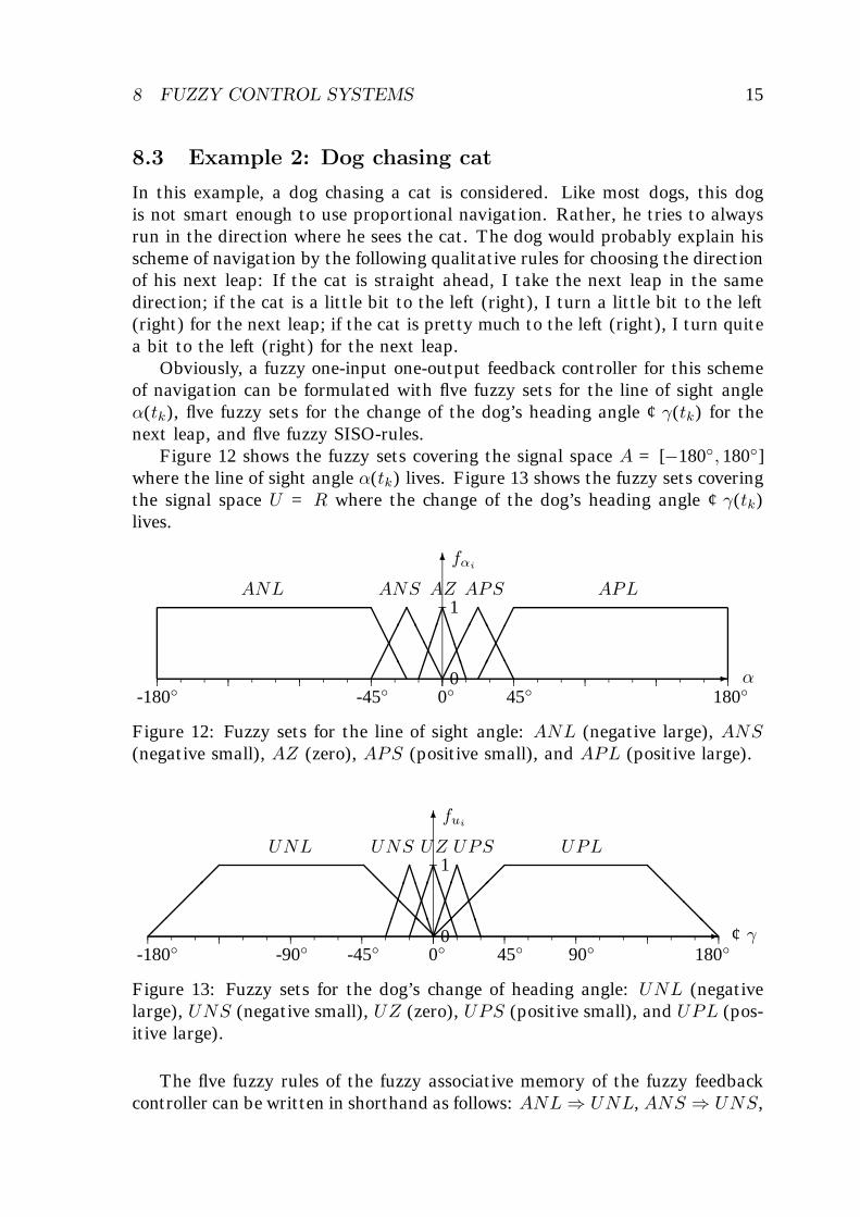
In this example, a dog chasing a cat is considered. Like most dogs, this dogis not smart enough to use proportional navigation. Rather, he tries to alwaysrun in the direction where he sees the cat. The dog would probably explain hisscheme of navigation by the following qualitative rules for choosing the directionof his next leap: If the cat is straight ahead, I take the next leap in the samedirection; if the cat is a little bit to the left (right), I turn a little bit to the left(right) for the next leap; if the cat is pretty much to the left (right), I turn quitea bit to the left (right) for the next leap.

Obviously, a fuzzy one-input one-output feedback controller for this schemeof navigation can be formulated with flve fuzzy sets for the line of sight angleα(tk), flve fuzzy sets for the change of the dog’s heading angle ¢γ(tk) for thenext leap, and flve fuzzy SISO-rules.

Figure 12 shows the fuzzy sets covering the signal space A = [−180◦, 180◦]where the line of sight angle α(tk) lives. Figure 13 shows the fuzzy sets coveringthe signal space U = R where the change of the dog’s heading angle ¢γ(tk)lives.

-

6

1

0-180◦ -45◦ 0◦ 45◦ 180◦

fαi

���

AAAA

APS

����

APL

AAAA

ANL

����

AAAA

ANS

����BBBB

AZ

Figure 12: Fuzzy sets for the line of sight angle: ANL (negative large), ANS(negative small), AZ (zero), APS (positive small), and APL (positive large).

-

6

1

0-180◦ -90◦ -45◦ 0◦ 45◦ 90◦ 180◦

fui

¢γ����BBBB

UPS

���� @

@@@

UPL

���� @

@@@

UNL

����BBBB

UNS

����BBBB

UZ

Figure 13: Fuzzy sets for the dog’s change of heading angle: UNL (negativelarge), UNS (negative small), UZ (zero), UPS (positive small), and UPL (pos-itive large).

The flve fuzzy rules of the fuzzy associative memory of the fuzzy feedbackcontroller can be written in shorthand as follows: ANL⇒ UNL, ANS ⇒ UNS,

16 GEERING: FUZZY CONTROL

AZ ⇒ UZ, APS ⇒ UPS, and APL ⇒ UPL. This should be read as follows:If α(tk) belongs to the fuzzy set ANL to degree d then the fuzzy set UNL forthe change of heading angle should be flred to degree d, etc.

Since it is not quite clear what the dog means by \turning a little bit" or\turning pretty much", a multiplicative doggy gain K is introduced. Further-more, it is assumed that the dog cannot change his heading angle by more than90◦ in either direction from one step to the next. This leads to the flnal controllaw

u(tk) = ¢γ(tk) = sat{KD{vu(tk)}} ,where vu(tk) is the fuzzy variable at the output of the fuzzy associative memoryat time tk (cf. Figure 4).

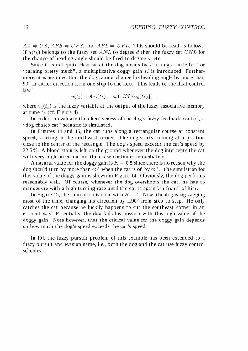
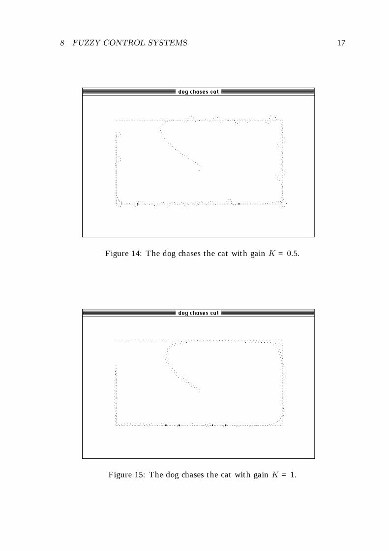
In order to evaluate the efiectiveness of the dog’s fuzzy feedback control, a\dog chases cat" scenario is simulated.

In Figures 14 and 15, the cat runs along a rectangular course at constantspeed, starting in the northwest corner. The dog starts running at a positionclose to the center of the rectangle. The dog’s speed exceeds the cat’s speed by32.5 %. A blood stain is left on the ground whenever the dog intercepts the catwith very high precision but the chase continues immediately.

A natural value for the doggy gain is K = 0.5 since there is no reason why thedog should turn by more than 45◦ when the cat is ofi by 45◦. The simulation forthis value of the doggy gain is shown in Figure 14. Obviously, the dog performsreasonably well. Of course, whenever the dog overshoots the cat, he has tomanoeuvre with a high turning rate until the cat is again \in front" of him.

In Figure 15, the simulation is done with K = 1. Now, the dog is zig-zaggingmost of the time, changing his direction by ±90◦ from step to step. He onlycatches the cat because he luckily happens to cut the southeast corner in ane–cient way. Essentially, the dog fails his mission with this high value of thedoggy gain. Note however, that the critical value for the doggy gain dependson how much the dog’s speed exceeds the cat’s speed.

In [9], the fuzzy pursuit problem of this example has been extended to afuzzy pursuit and evasion game, i.e., both the dog and the cat use fuzzy controlschemes.

8 FUZZY CONTROL SYSTEMS 17

Figure 14: The dog chases the cat with gain K = 0.5.

Figure 15: The dog chases the cat with gain K = 1.

18 GEERING: FUZZY CONTROL

9 Computational Issues

9.1 Efficient Defuzzification

Consider the task of simulating a fuzzy control system on a general purposedigital computer. For the simulation of the fuzzy (feedback) controller, Figures4 and 5 suggest that the following sequence of operations should be executed atevery sampling time:

• Fuzzify each of the error signals ei to the corresponding fuzzy vector vei :vei = F(ei).

• Evaluate all of the fuzzy rules deflned for the fuzzy controller. Each of thefuzzy rules yields a fuzzy variable vj which is represented by the modulatedfunction gj(u).

• Calculate the sum of all of these fuzzy variables vj in order to get thefuzzy control variable vu =

∑j vj which is represented by the function

g(u) =∑j gj(u).

• Defuzzify the fuzzy control variable vu by calculating its centroid u:

u = D(vu) =∫ug(u)du∫g(u)du

.

Notice that for piecewise linear functions gj(u), the sum g(u) is also a piece-wise linear function and both of the integrals of the defuzziflcation operation canbe calculated analytically. Therefore, using fuzzy sets with piecewise linear setmembership functions only (such as \triangles", \trapezoids", or piecewise lin-ear approximations of more sophisticated smooth functions) can lead to rathere–cient program code.

In order to further reduce the run time of the simulation signiflcantly, theresult of the following lemma is needed.

Consider the modulated functions gj , j = 1, . . . , N , and the correspondingfunction g =

∑Nj=1 gj of the fuzzy control signal vu. Let wgj and cgj be the

weights and the centroids, respectively, of the modulated functions gj , i.e.,

wgj =∫gj(u) du

and

cgj =

∫ugj(u) du∫gj(u) du

=1wgj

∫ugj(u) du .

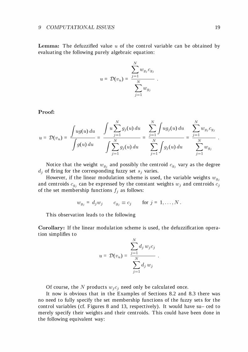
9 COMPUTATIONAL ISSUES 19

Lemma: The defuzzifled value u of the control variable can be obtained byevaluating the following purely algebraic equation:

u = D(vu) =

N∑j=1

wgjcgj

N∑j=1

wgj

.

Proof:

u = D(vu) =

∫ug(u) du∫g(u) du

=

∫u

N∑j=1

gj(u) du

∫ N∑j=1

gj(u) du

=

N∑j=1

∫ugj(u) du

N∑j=1

∫gj(u) du

=

N∑j=1

wgjcgj

N∑j=1

wgj

.

Notice that the weight wgj and possibly the centroid cgj vary as the degreedj of flring for the corresponding fuzzy set sj varies.

However, if the linear modulation scheme is used, the variable weights wgjand centroids cgj can be expressed by the constant weights wj and centroids cjof the set membership functions fj as follows:

wgj = djwj cgj ≡ cj for j = 1, . . . , N .

This observation leads to the following

Corollary: If the linear modulation scheme is used, the defuzziflcation opera-tion simplifles to

u = D(vu) =

N∑j=1

dj wjcj

N∑j=1

dj wj

.

Of course, the N products wjcj need only be calculated once.It now is obvious that in the Examples of Sections 8.2 and 8.3 there was

no need to fully specify the set membership functions of the fuzzy sets for thecontrol variables (cf. Figures 8 and 13, respectively). It would have su–ced tomerely specify their weights and their centroids. This could have been done inthe following equivalent way:

20 GEERING: FUZZY CONTROL

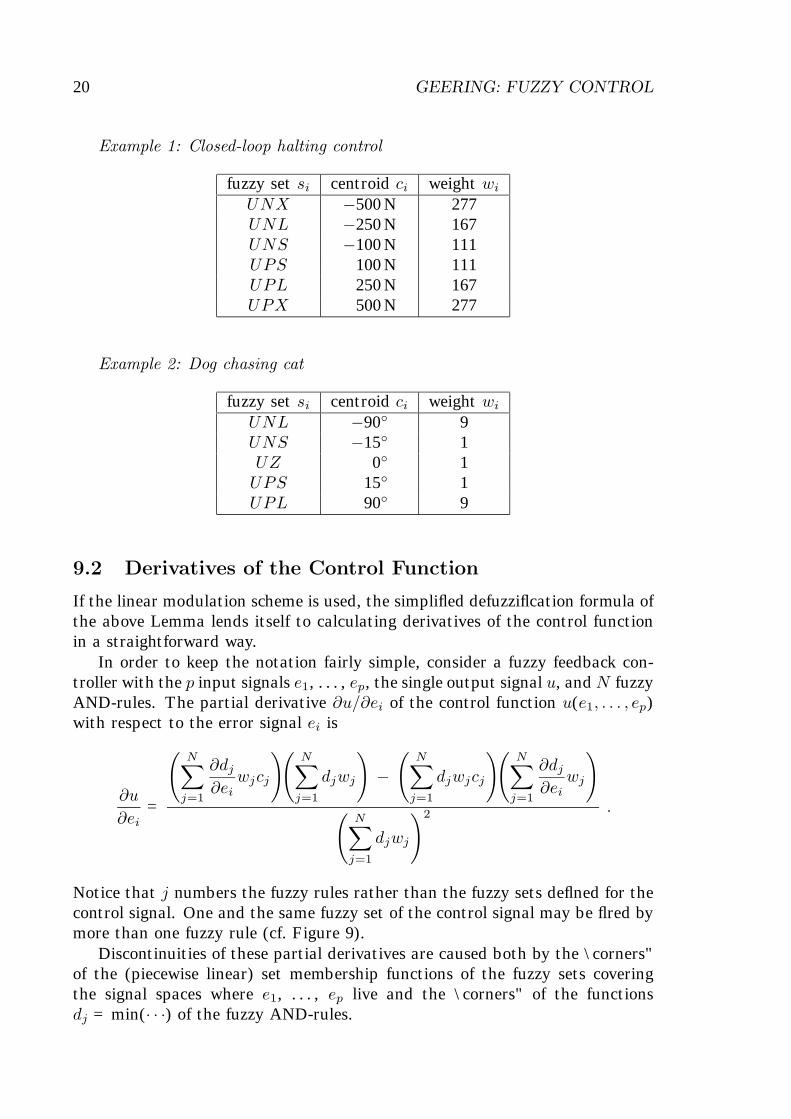
Example 1: Closed-loop halting control

fuzzy set si centroid ci weight wiUNX −500 N 277UNL −250 N 167UNS −100 N 111UPS 100 N 111UPL 250 N 167UPX 500 N 277

Example 2: Dog chasing cat

fuzzy set si centroid ci weight wiUNL −90◦ 9UNS −15◦ 1UZ 0◦ 1UPS 15◦ 1UPL 90◦ 9

9.2 Derivatives of the Control Function

If the linear modulation scheme is used, the simplifled defuzziflcation formula ofthe above Lemma lends itself to calculating derivatives of the control functionin a straightforward way.

In order to keep the notation fairly simple, consider a fuzzy feedback con-troller with the p input signals e1, . . . , ep, the single output signal u, andN fuzzyAND-rules. The partial derivative ∂u/∂ei of the control function u(e1, . . . , ep)with respect to the error signal ei is

∂u

∂ei=

(N∑j=1

∂dj∂ei

wjcj

)(N∑j=1

djwj

)−(

N∑j=1

djwjcj

)(N∑j=1

∂dj∂ei

wj

)(

N∑j=1

djwj

)2 .

Notice that j numbers the fuzzy rules rather than the fuzzy sets deflned for thecontrol signal. One and the same fuzzy set of the control signal may be flred bymore than one fuzzy rule (cf. Figure 9).

Discontinuities of these partial derivatives are caused both by the \corners"of the (piecewise linear) set membership functions of the fuzzy sets coveringthe signal spaces where e1, . . . , ep live and the \corners" of the functionsdj = min(· · ·) of the fuzzy AND-rules.

9 COMPUTATIONAL ISSUES 21

9.3 Observations and Suggestions

For the sake of simplicity, consider a fuzzy SISO feedback controller. From theformulae for the defuzziflcation operator and for the derivative of the controlfunction, the following observations and suggestions ensue:

• If none of the fuzzy sets of the control signal u is flred to a strictly positivedegree, the value of the defuzzifled control signal is undeflned. Therefore,the signal space E, where the error signal e lives, must be covered com-pletely by its collection of fuzzy sets, and these fuzzy sets should overlap.In other words, every error e ∈ E should belong to at least one fuzzy set toa strictly positive degree. Furthermore, in the associative memory, everyfuzzy set of the error signal should flre (at least) one of the fuzzy sets ofthe control signal.

• If two neighbouring fuzzy sets of the error signal \touch" at e1 but do notoverlap, the control function is discontinuous at e1. For e = e1, the resultof the defuzziflcation operator is undeflned. The value of the control signalmust be deflned separately. | In Example 1 (fuzzy halting control), theanalogous situation occurs for ep = ev = 0. The obvious extra deflnitionis uc(0, 0) = 0.

• Assume that the linear modulation scheme is applied. If in some interval[ea, eb] ⊂ E the error e belongs to exactly one fuzzy set to a strictly positivedegree, the control function is constant on this interval, irrespective of theshape of this fuzzy set for the error signal. | In Example 2 (dog chasingcat), the dog will turn by ¢γ = sat{K · 15◦} if the line of sight angle αis in the interval [15◦, 22.5◦], or by ¢γ = sat{K · 90◦} if the line of sightangle exceeds 45◦. (Obviously, the dog could improve his performancesigniflcantly by choosing the centroids +45◦ and −45◦ for the fuzzy setsUPL and UNL, respectively, and the doggy gain K = 1.)

• Assume that the linear modulation scheme is applied. For the purpose ofimplementing a flnished design of a fuzzy controller, only the weights wiand the centroids ci of the fuzzy sets for the control signals are needed inthe defuzziflcation operation (cf. Section 9.1). | On the other hand, thecomplete speciflcations of the set membership functions of the fuzzy setsfor the control signals are needed, if the fuzzy rules of the controller mustbe \learnt" by watching an expert performing the task at hand. This topicis beyond the scope of this report. The interested reader is referred to [1],and [8], and the references cited there.

• In Section 8, \static" fuzzy controllers are considered only. The readershould have no problem in extending these ideas to fuzzy controllers incor-porating \dynamic compensation". In the simplest case the input signalsof the fuzzy dynamic compensator include the most recent error signals

22 GEERING: FUZZY CONTROL

ei(k) and the delayed error signals ei(k−1), ei(k−2), etc., and perhapspreviously issued control signals uj(k−1), uj(k−2) etc.. In the latter case itis e–cient to refuzzify the defuzzifled control signals in order to obtain therequired delayed fuzzy control variables. All or most of the processing isperformed in the fuzzy part of the controller. In more sophisticated cases,non-fuzzy dynamic compensation (e.g., in the form of a full state observer)can be performed in a preprocessor to the fuzzy controller proper.

References

[1] B. Kosko, Neural Networks and Fuzzy Systems: A Dynamical Systems Ap-proach to Machine Intelligence, Prentice-Hall, Englewood Clifis, NJ, USA,1992.

[2] H.-J. Zimmermann, Fuzzy Set Theory and its Applications, 2nd ed., Kluwer,Boston, MA, USA, 1991.

[3] W. Pedrycz, Fuzzy Control and Fuzzy Systems, Electronic & Electrical En-gineering Research Studies, Control Theory and Applications Series, vol. 3,Research Studies Press (Wiley), Taunton, Somerset, England, 1989.

[4] D. J. Dubois, H. M. Prade, Fuzzy Sets and Systems, Academic Press, NewYork, NY, 1980.

[5] L. A. Zadeh, Fuzzy Sets and Applications: Selected Papers, Wiley-Inter-science, New York, NY, USA, 1987.

[6] M. M. Gupta, T. Yamakawa, (eds.), Fuzzy Computing, Hardware, and Ap-plications, North-Holland, Amsterdam, Netherlands, 1988.

[7] M. Sugeno, (ed.), Industrial Applications of Fuzzy Control, North-Holland,Amsterdam, Netherlands, 1985.

[8] C.-T. Lin, C. S. G. Lee, \Neural-Network-Based Fuzzy Logic Controland Decision Systems," IEEE Transactions on Computers, vol. 40(1991),pp. 1320{1336.

[9] S. Ginsburg, R. Wimmer, H. P. Geering, \Clever Dog versus Smart Cat,"Proceedings of the International ICSC Symposium on Fuzzy Logic, pp. A99{A104, Zurich, Switzerland, May, 1995.

[10] H. Kiendl, Fuzzy Control methodenorientiert, Oldenbourg, Munich, Ger-many, 1997.