Embed Size (px)
Citation preview
Interprocedural AnalysisMooly Sagiv
http://www.math.tau.ac.il/~sagiv/courses/pa.html
Tel Aviv University
640-6706
Sunday 18-21 Scrieber 8
Monday 10-12 Schrieber 317
Textbook Chapter 2.5
Outline The trivial solution Why isn’t it adequate Challenges in interprocedural analysis Simplifying assumptions A naive solution Join over valid paths The functional approach
– A case study linear constant propagation
– Context free reachability The call-string approach Modularity issues
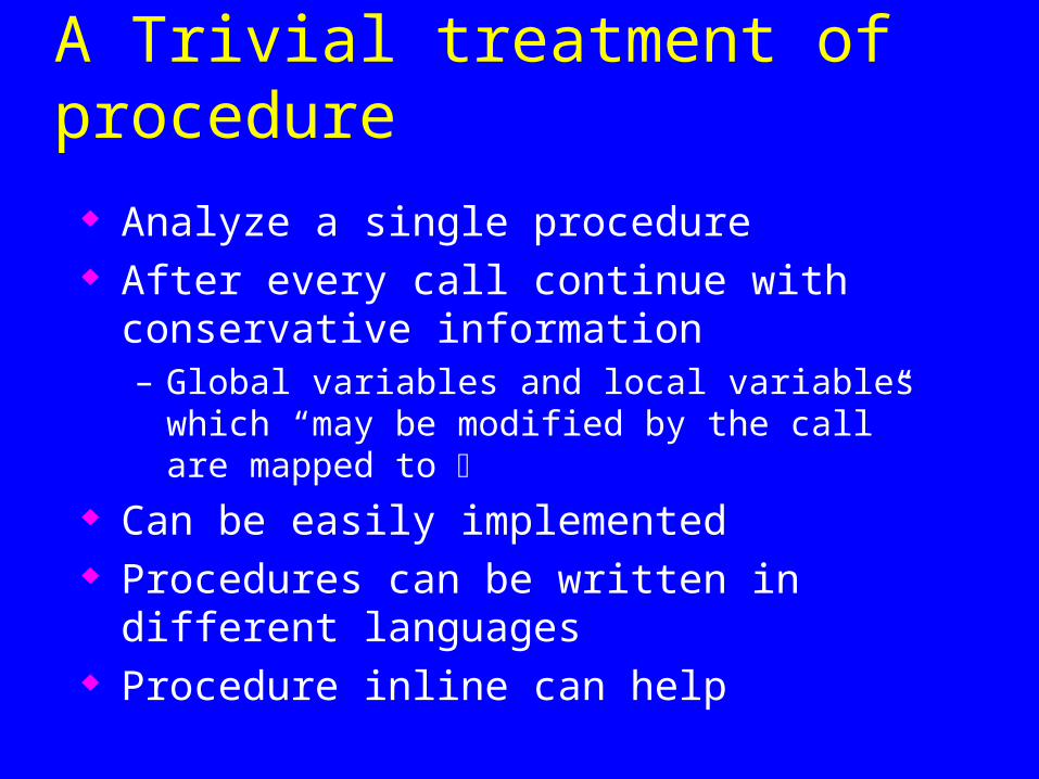
A Trivial treatment of procedure
Analyze a single procedure After every call continue with conservative
information– Global variables and local variables which “may be
modified by the call” are mapped to Can be easily implemented Procedures can be written in different languages Procedure inline can help
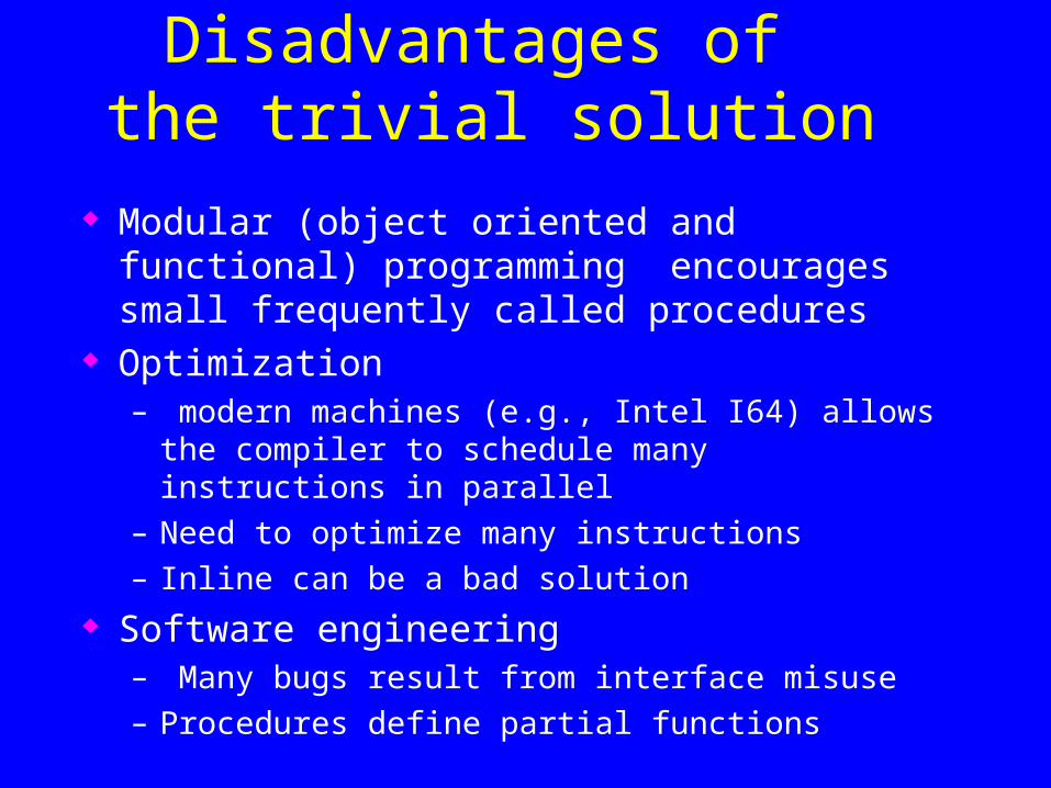
Disadvantages of the trivial solution
Modular (object oriented and functional) programming encourages small frequently called procedures
Optimization– modern machines (e.g., Intel I64) allows the compiler
to schedule many instructions in parallel
– Need to optimize many instructions
– Inline can be a bad solution
Software engineering– Many bugs result from interface misuse
– Procedures define partial functions
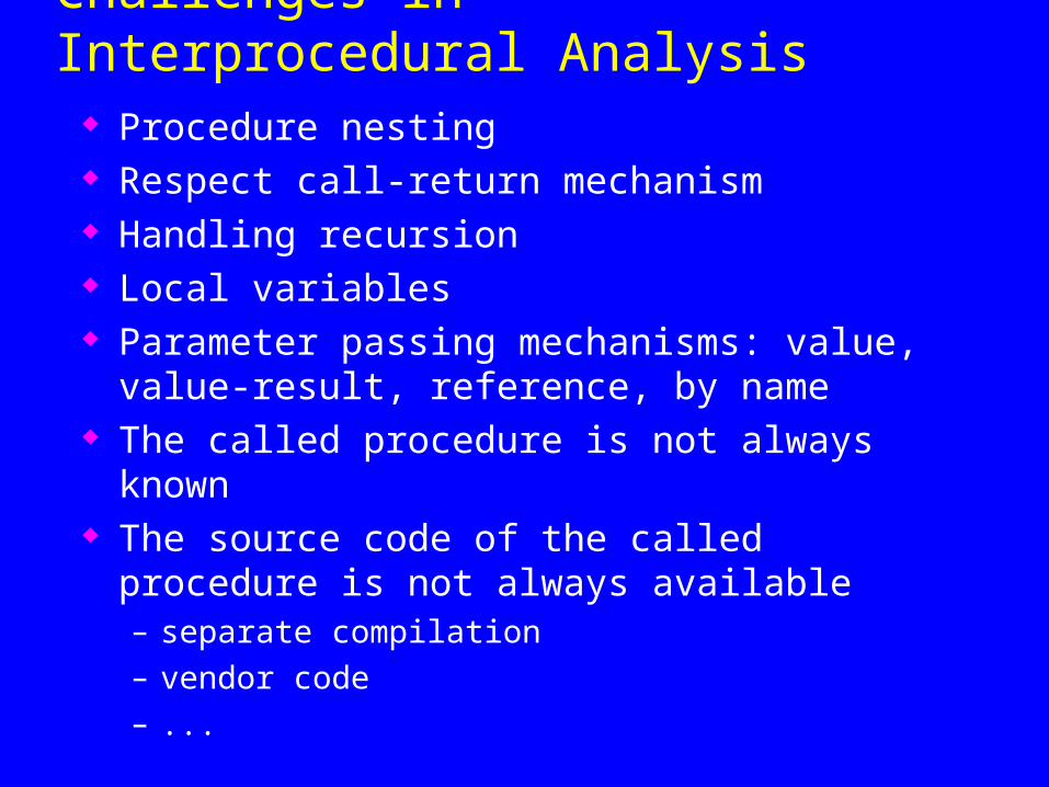
Challenges in Interprocedural Analysis Procedure nesting Respect call-return mechanism Handling recursion Local variables Parameter passing mechanisms: value, value-
result, reference, by name The called procedure is not always known The source code of the called procedure is not
always available – separate compilation
– vendor code
– ...
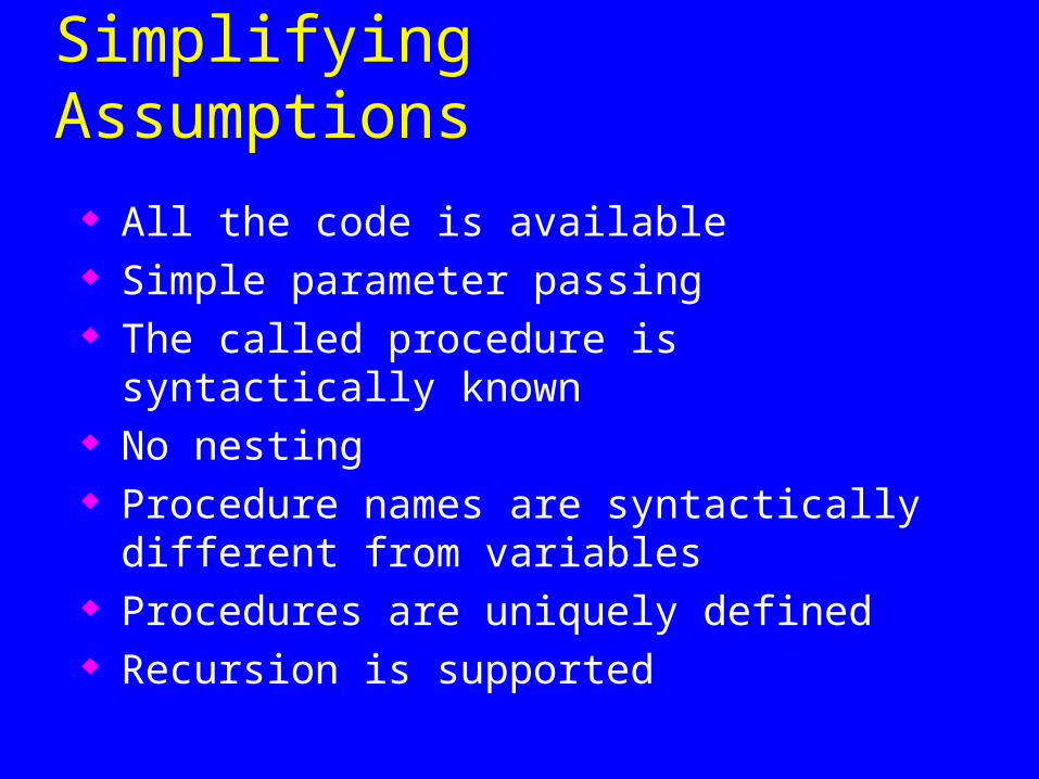
Simplifying Assumptions
All the code is available Simple parameter passing The called procedure is syntactically known No nesting Procedure names are syntactically different from
variables Procedures are uniquely defined Recursion is supported
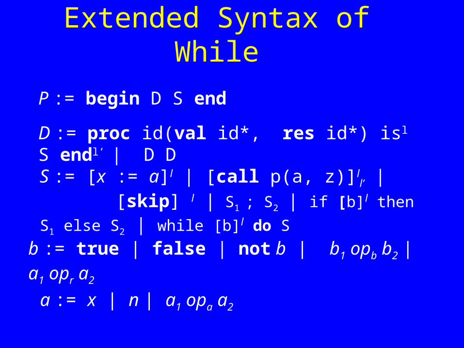
Extended Syntax of While
a := x | n | a1 opa a2
b := true | false | not b | b1 opb b2 | a1 opr a2
S := [x := a]l | [call p(a, z)]ll’ |
[skip] l | S1 ; S2 | if [b]l then S1 else S2 | while [b]l do S
P := begin D S end
D := proc id(val id*, res id*) isl S endl’ | D D
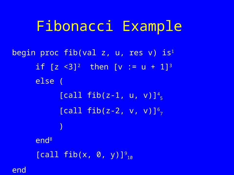
Fibonacci Example
begin proc fib(val z, u, res v) is1
if [z <3]2 then [v := u + 1]3
else (
[call fib(z-1, u, v)]45
[call fib(z-2, v, v)]67
)
end8
[call fib(x, 0, y)]910
end

Constant Example
begin proc p(val a) is1
if [b]2 then (
[a := a -1]3
[call p(a)]45
[a := a + 1]6
)
[x := -2* a + 5]7
end8
[call p(7)]910
end
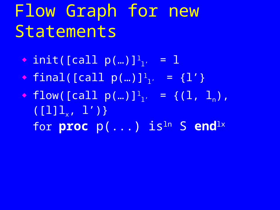
Flow Graph for new Statements
init([call p(…)]ll’ = l
final([call p(…)]ll’ = {l’}
flow([call p(…)]ll’ = {(l, ln), ([l]lx, l’)}
for proc p(...) isln S endlx
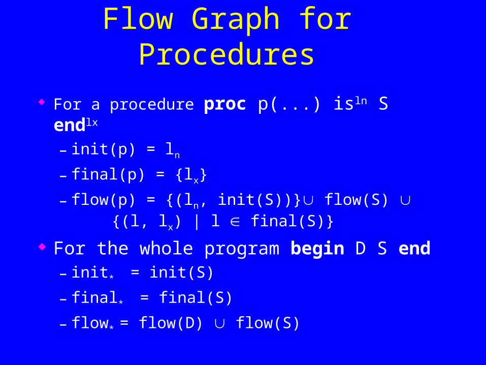
Flow Graph for Procedures
For a procedure proc p(...) isln S endlx
– init(p) = ln
– final(p) = {lx}
– flow(p) = {(ln, init(S))} flow(S) {(l, lx) | l final(S)}
For the whole program begin D S end– init* = init(S)
– final* = final(S)
– flow* = flow(D) flow(S)
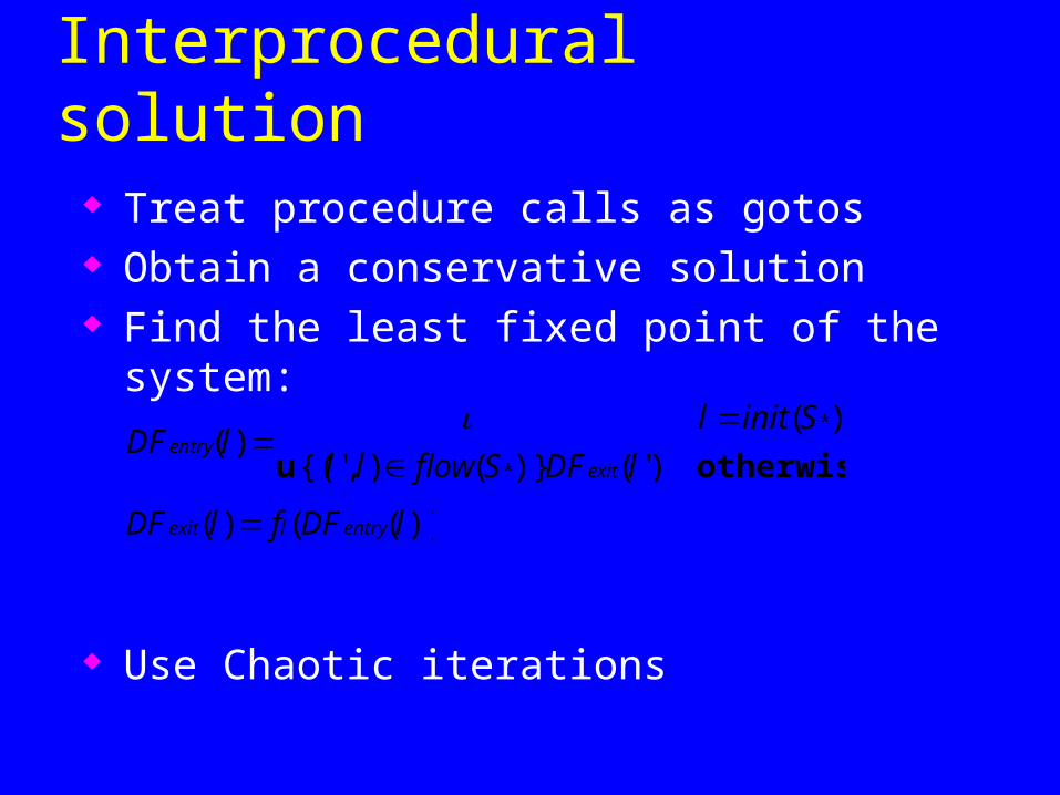
A naive Interprocedural solution Treat procedure calls as gotos Obtain a conservative solution Find the least fixed point of the system:
Use Chaotic iterations
otherwise u )'()}(),'{(
)()(
*
*
lDFSflowll
SinitllDF
exitentry
))(()( lDFflDF entrylexit
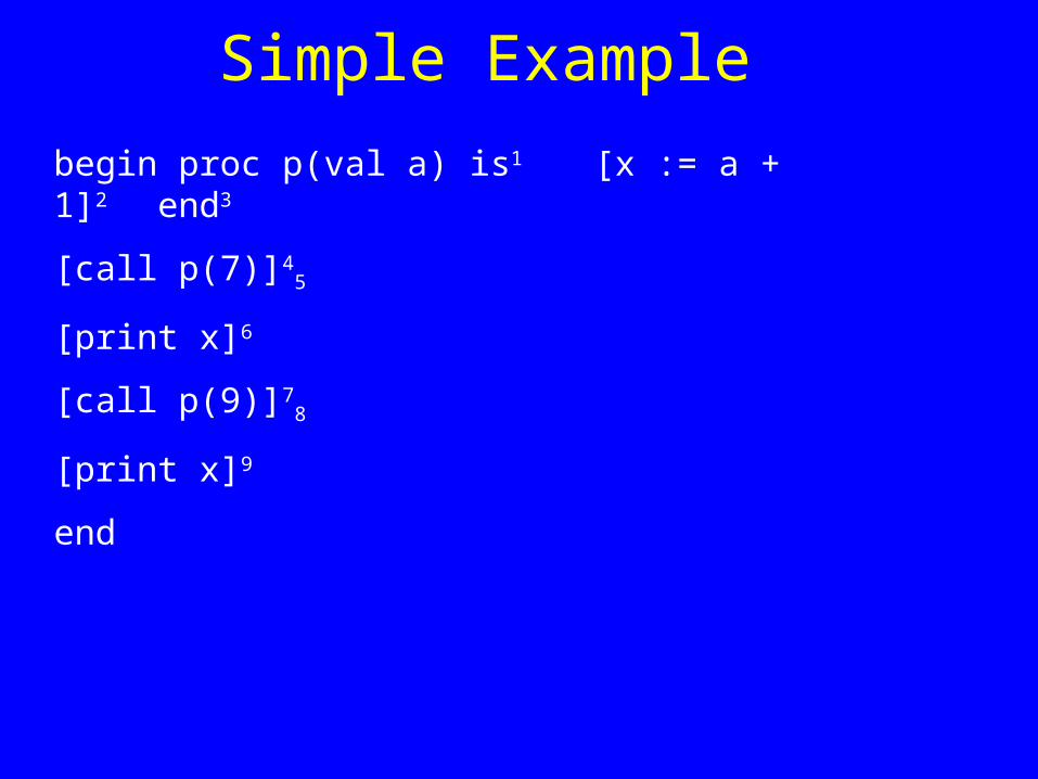
Simple Example
begin proc p(val a) is1 [x := a + 1]2 end3
[call p(7)]45
[print x]6
[call p(9)]78
[print x]9
end
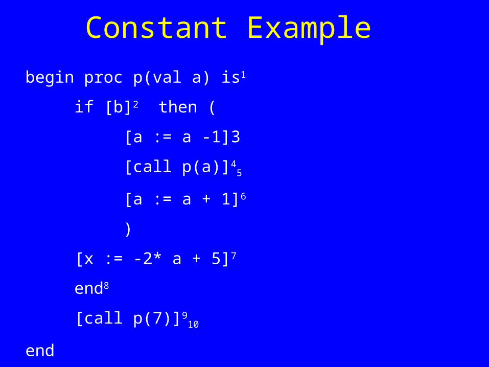
Constant Example
begin proc p(val a) is1
if [b]2 then (
[a := a -1]3
[call p(a)]45
[a := a + 1]6
)
[x := -2* a + 5]7
end8
[call p(7)]910
end
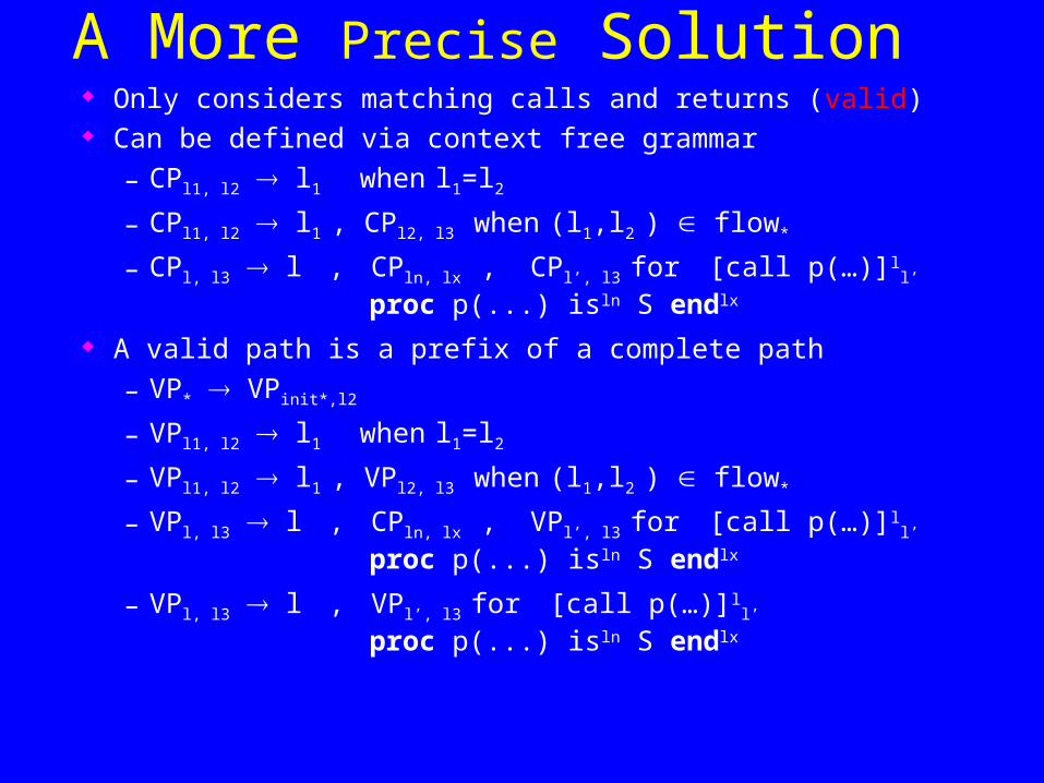
A More Precise Solution Only considers matching calls and returns (valid) Can be defined via context free grammar
– CPl1, l2 l1 when l1=l2
– CPl1, l2 l1 , CPl2, l3 when (l1,l2 ) flow*
– CPl, l3 l , CPln, lx , CPl’, l3 for [call p(…)]ll’
proc p(...) isln S endlx
A valid path is a prefix of a complete path
– VP* VPinit*,l2
– VPl1, l2 l1 when l1=l2
– VPl1, l2 l1 , VPl2, l3 when (l1,l2 ) flow*
– VPl, l3 l , CPln, lx , VPl’, l3 for [call p(…)]ll’
proc p(...) isln S endlx
– VPl, l3 l , VPl’, l3 for [call p(…)]ll’
proc p(...) isln S endlx
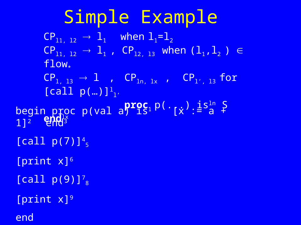
Simple Example
begin proc p(val a) is1 [x := a + 1]2 end3
[call p(7)]45
[print x]6
[call p(9)]78
[print x]9
end
CPl1, l2 l1 when l1=l2
CPl1, l2 l1 , CPl2, l3 when (l1,l2 ) flow*
CPl, l3 l , CPln, lx , CPl’, l3 for [call p(…)]ll’
proc p(...) isln S endlx
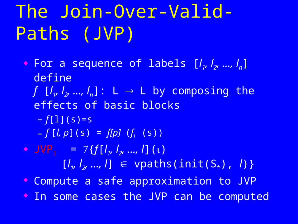
The Join-Over-Valid-Paths (JVP)
For a sequence of labels [l1, l2, …, ln] definef [l1, l2, …, ln]: L L by composing the effects of basic blocks– f[l](s)=s
– f [l, p](s) = f[p] (fl (s))
JVPl = {f[l1, l2, …, l]() [l1, l2, …, l] vpaths(init(S*), l)}
Compute a safe approximation to JVP In some cases the JVP can be computed
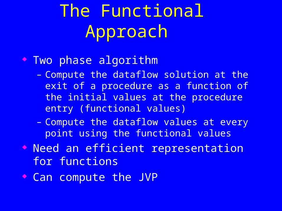
The Functional Approach
Two phase algorithm– Compute the dataflow solution at the exit of a
procedure as a function of the initial values at the procedure entry (functional values)
– Compute the dataflow values at every point using the functional values
Need an efficient representation for functions Can compute the JVP
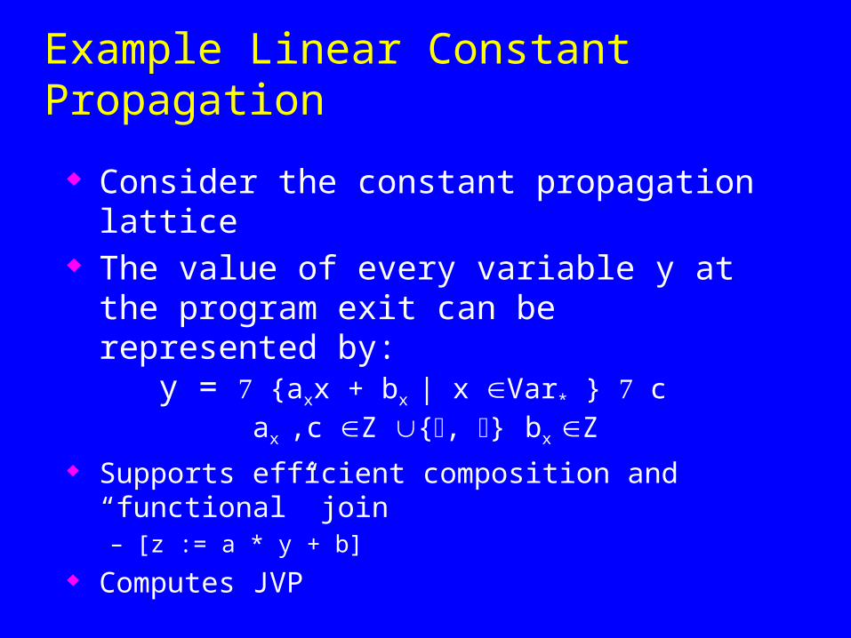
Example Linear Constant Propagation
Consider the constant propagation lattice The value of every variable y at the program exit
can be represented by: y = {axx + bx | x Var* } c ax ,c Z {, } bx Z
Supports efficient composition and “functional” join– [z := a * y + b]
Computes JVP

Constant Example
begin proc p(val a) is1
if [b]2 then (
[a := a -1]3
[call p(a)]45
[a := a + 1]6
)
[x := -2* a + 5]7
end8
[call p(7)]910
end

Functional Approach via Context Free Reachablity
The problem of computing reachability in a graph restricted by a context free grammar can be solved in cubic time
Can be used to compute JVP in arbitrary finite distributive data flow problems (not just bitvector)
Nodes in the graph correspond to individual facts
The Call String Approach for Approximating JVP
No assumptions Record at every label a pair (l, c) where l L is
the dataflow information and c is a suffix of unmatched calls
Use Chaotic iterations To guarantee termination limit the size of c
(typically 1 or 2) Emulates inline Exponential in C

Constant Example
begin proc p(val a) is1
if [b]2 then (
[a := a -1]3
[call p(a)]45
[a := a + 1]6
)
[x := -2* a + 5]7
end8
[call p(7)]910
end