Interpolation methods for spatio-temporal geographic data

Interpolation methods for spatio-temporalgeographic data

Lixin Li, Peter Revesz*

Computer Science and Engineering Department, University of Nebraska-Lincoln, Lincoln, NE 68588, USA

Abstract

We consider spatio-temporal interpolation of geographic data using both the reductionmethod, which treats time as an independent dimension, and the extension method, which

treats time as equivalent to a spatial dimension. We adopt both 2-D and 3-D shape functionsfrom finite element methods for the spatio-temporal interpolation of 2-D spatial and 1-Dtemporal data sets. We also develop new 4-D shape functions and use them for the spatio-temporal interpolation of 3-D spatial and 1-D temporal data sets. Using an actual real estate

data set with house prices, we compare these methods with other spatio-temporal interpola-tion methods based on inverse distance weighting and kriging. The comparison criteriainclude interpolation accuracy, error-proneness to time aggregation, invariance to scaling on

the coordinate axes, and the type of constraints used in the representation of the interpolateddata. Our experimental results show that the extension method based on shape functions isthe most accurate and the overall best spatio-temporal interpolation method. New color ren-

dering algorithms are also developed for the visualization of time slices of the interpolatedspatio-temporal data. We show some visualization results of the real estate data set includingthe vertical profile of house prices.# 2003 Elsevier Ltd. All rights reserved.

Keywords: Spatio-temporal interpolation; Shape functions; Constraint databases

1. Introduction

Geographic information system (GIS) applications often require spatio-temporalinterpolation of an input data set. Spatio-temporal interpolation requires the esti-mation of the unknown values at unsampled location-time pairs with a satisfyinglevel of accuracy. For example, suppose that we know the recording of temperatures

Computers, Environment and Urban Systems

28 (2004) 201–227

www.elsevier.com/locate/compenvurbsys

0198-9715/03/$ - see front matter # 2003 Elsevier Ltd. All rights reserved.

doi:10.1016/S0198-9715(03)00018-8

* Corresponding author. Tel.: +1-402-472-3488; fax: +1-402-472-7767.

E-mail addresses: [email protected] (P. Revesz), [email protected] (L. Li).

http://www.elsevier.com/locate/compenvurbsys/a4.3d

mailto:[email protected]

mailto:[email protected]

at different weather stations at different instances of time. Then spatio-temporalinterpolation would estimate the temperature at unsampled locations and times.

Spatial interpolation is already frequently used in GIS. There are many spatialinterpolation algorithms for spatial (2-D or 3-D) data sets. Shepard (1968) discussesin detail inverse distance weighting, Deutsch and Journel (1998) kriging, Goodmanand O’Rourke (1997) splines, Zurflueh (1967) trend surfaces, and Harbaugh andPreston (1968) Fourier series. Lam (1983) gives a review and comparison of spatialinterpolation methods.

There are surprisingly few papers that consider the topic of spatio-temporalinterpolation in GIS. In fact, we could only find papers in spatio-temporal inter-polation that estimate the motion of moving objects, which is a major concern inhuman vision but unrelated to GIS. One exception is Miller (1997, chapter 13),which utilizes kriging for spatio-temporal interpolation.

Most GIS researchers assume that spatio-temporal interpolation is reducible to asequence of spatial interpolations. This reduction is convenient only if we sample thesame locations at the same times. For example, this may be true for the above tem-perature data set if each weather station records the Monday noon temperature oneach Monday. Then we can do a separate spatial interpolation for each timeinstance for which we have the temperatures at the weather stations.

However, irregular data sets are also quite common. For example, consider a dataset that records the price of houses sold in a city. For each day of sale, this data setcan give us only the exact price of a set of houses (those that are sold that day). Thissubset varies day by day. This is unlike the set of weather stations which are fixed.For such irregular data sets the above reduction method is unnatural to apply.

The outline of our paper and our main contributions are the following.

(1) In Section 2 we give a literature review about using 2-D and 3-D shapefunctions to approach spatial interpolation problems.(2) In Section 3 we start by describing two general methods for spatio-temporalinterpolations. The reduction method treats time independently from the spatialdimensions. The extension method treats time as equivalent to a spatial dimension.(3) In Section 3.1 we consider 2-D space and 1-D time spatio-temporal inter-polation. We illustrate the reduction approach using a combination of 2-D shapefunctions for space and 1-D shape functions for time (Section 3.1.1). We alsoillustrate the extension approach using 3-D shape functions where the first twodimensions are for space and the third dimension is for time (Section 3.1.2). Inboth cases we consider visualization of the spatio-temporal interpolation. For thereduction method we give a new color rendering scheme which utilizes 1-D shapefunctions.(4) In Section 3.2 we consider 3-D space and 1-D time spatio-temporal inter-polation. For the reduction method we use the combination of 3-D shape func-tions for space and 1-D shape functions for time (Section 3.2.1). For the extensionmethod we first divide the 4-D domain by a 4-D Delaunay Tesselation (see Section2.3). Then we develop new 4-D (Section 3.2.2) shape functions that can be appliedfor each 4-D Delaunay Tesselation element.

202 L. Li, P. Revesz / Comput., Environ. and Urban Systems 28 (2004) 201–227

(5) Section 4 compares our interpolation methods with the inverse distance weightingand kriging methods based on the same actual real estate data. We show that theextension method with shape functions is the most accurate spatio-temporal inter-polation method as measured by mean absolute error (MAE) and root mean squareerror (RMSE). It is also the only one which can be represented using linear constraints.The extension method, which treats time as another dimension, has a potentialproblem, namely that there is no easy way to compare one temporal unit with onespatial unit. Depending on the unit measure, we may get a different value for theestimated results. Are there spatio-temporal interpolations that are invariant withrespect to the choice of units in the spatial and temporal axes? We show that onlyshape functions-based spatio-temporal interpolation are invariant.Finally, in the real estate data instead of recording the precise date of sale ofhouses we may have only records of monthly, bimonthly or even yearly sales, thatis, all the houses sold in that time interval are listed together. We show experi-mentally that this time aggregation has a serious negative effect on the accuracy ofthe reduction method, while the extension method is barely affected.(6) In Section 5 we give an example of using 4-D shape functions by considering anextension of the real estate data where the height of each house is also recorded.(7) Finally, in Section 6 we discuss some future work.

2. Literature review

In this section, we give a literature review about 2-D and 3-D shape functions aswell as 4-D Delaunay tesselation. Shape functions, which can be viewed as a spatialinterpolation method, are popular in engineering applications, for example, in finiteelement algorithms (Buchanan, 1995; Zienkiewics & Taylor, 2000). There arevarious types of 2-D and 3-D shape functions. In this section, we are only interestedin 2-D shape functions for triangles and 3-D shape functions for tetrahedra, both ofwhich are linear approximation methods.

2.1. 2-D shape functions for triangles

2.1.1. Triangular meshesWhen dealing with complex geometric domains, it is convenient to divide the total

domain into a finite number of simple sub-domains which can have triangular orquadrilateral shapes in the case of 2-D problems. Mesh generation using triangularor quadrilateral domains is important in finite element discretization of engineeringproblems. For the generation of triangular meshes, quite successful algorithms havebeen developed. A popular method for the generation of triangular meshes is the‘‘Delaunay Triangulation’’ (Goodman & O’Rourke, 1997; Preparata & Shamos,1985; Shewchuk, 1996). We embedded in our system the Delauney triangulationalgorithm available from the public Website http://www.geom.umn.edu/software/�qhull and used this for one of our spatio-temporal data approximation methodswhich will be described in Section 3.1.1.

L. Li, P. Revesz / Comput., Environ. and Urban Systems 28 (2004) 201–227 203

2.1.2. Linear approximation in 2-D spaceA linear approximation function for a triangular area can be written in terms of

three shape functions N1, N2, N3, and the corner values w1, w2, w3. In Fig. 1, two tri-angular finite elements, I and II, are combined to cover the whole domain considered.

In this example, the function in the whole domain is interpolated using four discretevalues w1, w2, w3, and w4 at four locations. A particular feature of the chosenapproximation method is that the function values inside the sub-domain I can beobtained by using only the three corner values w1, w2 and w3, whereas all functionvalues for the sub-domain II can be constructed using the corner values w2, w3, andw4. The linear interpolation function for the sub-domain of element I can be written as

w x; yð Þ ¼ N1 x; yð Þw1 þN2 x; yð Þw2 þN3 x; yð Þw3 ¼ N1N2N3½ �

w1

w2

w3

24

35 ð1Þ

where N1, N2 and N3 are the following shape functions:

N1 x; yð Þ ¼x2y3 � x3y2ð Þ þ x y2 � y3ð Þ þ y x3 � x2ð Þ½ �

2A


2A


2A: ð2Þ

The area A of element II in Eq. (2) can be computed using the corner coordinatesxi; yið Þ i ¼ 1; 2; 3ð Þ in the determinant of a 33 matrix according to

A ¼1

2det

1 x1 y1

1 x2 y2

1 x3 y3

24

35: ð3Þ

It should be noted that for every sub-domain, a local approximation functionsimilar to expression (1) is used. Each local approximation function is constrained tothe local triangular sub-domain. For example, the function w of Eq. (1) is valid only

Fig. 1. Linear interpolation in space for triangular elements.


for sub-domain I. For sub-domain II, the local approximation takes a similar formas the expression (1): we just have to replace the corner values w1, w2 and w3 withthe new values w2, w3 and w4.

Alternatively, considering only sub-domain I, the 2-D shape function (2) can alsobe expressed as follows (Revesz & Li, 2002b)

N1 x; yð Þ ¼ A1

A;N2 x; yð Þ ¼ A2

A;N3 x; yð Þ ¼ A3

A; ð4Þ

where A1, A2 and A3 are the three sub-triangle areas of sub-domain I as shown inFig. 2, and A is the area of the outside triangle w1w2w3 which can be computed byEq. (3). All the Ais (14i43) can also be computed similarly to Eq. (3) by using theappropriate coordinate values.

2.2. 3-D shape functions for tetrahedra

2.2.1. Tetrahedral meshesThree-dimensional domains can be divided into a finite number of simple sub-

domains. For example, we can use tetrahedral or hexahedral sub-domains. Tetra-hedral meshing is of particular interest. With a large number of tetrahedral elements,we can also approximate complicated 3-D objects. Fig. 3 shows a tetrahedral meshof a 3-D object. This object has a cutout (one quarter of a cylinder) behind theboundary defined by the points ABCD.

There exist several methods to generate automatic tetrahedral meshes, such as the3-D Delaunay tetrahedrilization and some tetrahedral mesh improvement methodsto avoid poorly shaped tetrahedra. For example, the tetrahedral mesh generation byDelaunay refinement (Shewchuk, 1998) and tetrahedral mesh improvement usingswapping and smoothing (Freitag & Gooch, 1997).

Fig. 2. Computing shape functions by area divisions.


2.2.2. Linear approximation in 3-D spaceA linear approximation function for a 3-D tetrahedral element can be written in

terms of four shape functions N1, N2, N3, N4 and the corner values w1, w2, w3, w4. InFig. 4, two tetrahedral elements, I and II, cover the whole domain considered.

In this example, the function in the whole domain is interpolated using five discretevalues w1, w2, w3, w4, and w5 at five locations in space. To obtain the function valuesinside the tetrahedral element I, we can use the four corner values w1, w2, w3 and w4.Similarly, all function values for element II can be constructed using the corner valuesw1, w3, w4 and w5. The linear interpolation function for element I can be written as:

w x; y; zð Þ ¼ N1 x; y; zð Þw1 þN2 x; y; zð Þw2 þN3 x; y; zð Þw3 þN4 x; y; zð Þw4

¼ N1N2N3N4½ �

w1

w2

w3

w4

2664

3775 ð5Þ

where N1, N2 N3 and N4 are the following shape functions:

N1 x; y; zð Þ ¼a1 þ b1xþ c1yþ d1z

6V;N2 x; y; zð Þ ¼

a2 þ b2xþ c2yþ d2z

6V;

N3 x; y; zð Þ ¼a3 þ b3xþ c3yþ d3z

6V;N4 x; y; zð Þ ¼

a4 þ b4xþ c4yþ d4z

6V: ð6Þ

Fig. 3. A tetrahedral mesh.


The volume V of the tetrahedron used for the shape functions in (6) can becomputed using the corner coordinates xi; yi; zið Þ i ¼ 1; 2; 3; 4ð Þ in the determinant ofa 44 matrix according to

Fig. 4. Linear interpolation in space for tetrahedral elements.

V ¼1

6det

1 x1 y1 z1

1 x2 y2 z2

1 x3 y3 z3

1 x4 y4 z4

2664

3775: ð7Þ

By expanding the other relevant determinants into their cofactors, we have

a1 ¼ detx2 y2 z2

x3 y3 z3

x4 y4 z4

24

35 b1 ¼ �det

1 y2 z2

1 y3 z3

1 y4 z4

24

35

c1 ¼ �detx2 1 z2

x3 1 z3

x4 1 z4

24

35 d1 ¼ �det

x2 y2 1x3 y3 1x4 y4 1

24

35

with the other constants defined by cyclic interchange of the subscripts in the order4, 1, 2 ,3 (Zienkiewics & Taylor, 1989).

Alternatively, considering only the tetrahedral element I, the 3-D shape function(6) can also be expressed as follows:

N1 x; y; zð Þ ¼ V1

V;N2 x; y; zð Þ ¼ V2

V;N3 x; y; zð Þ ¼ V3

V ;N4 x; y; zð Þ ¼ V4

Vð8Þ


2, V3 and V4 are the volumes of the four sub-tetrahedra ww2w3w4, w1ww3w4,
V1, Vw1w2ww4, and w1w2w3w, respectively, as shown in Fig. 5; and V is the volume ofthe outside tetrahedron w1w2w3w4 which can be computed by Eq. (7). All theV is (14i44) can also be computed similarly to Eq. (7) by using the appropriatecoordinate values.
2.3. 4-D Delaunay tesselation

The Delaunay tesselation in 4-D space is a special case of n-D space Delaunaytesselation when n=4. The n-D Delaunay tesselation is defined as a space-fillingaggregate of n-simplices (Watson, 1981). Each Delaunay n-simplex can be repre-sented by an (n+1)-tuple of indices to the data points. We can use Matlab to com-pute the n-D Delaunay tesselation by function delaunayn. T ¼ delaunayn Xð Þ

computes a set of n-simplices such that no data points of X are contained in any n-Dhyperspheres of the n-simplices. The set of n-simplices forms the n-D Delaunay tes-sellation. X is an mn array representing m points in n-D space. T is an s nþ 1ð Þ

array where s is the number of n-simplices after the n-D Delaunay tesselation. Eachrow of T contains the indices into X of the vertices of the corresponding n-simplex.In order to solve 4-D Delaunay tesselation in Matlab, we need to give the delaunaynfunction proper X array with size m4. An example of a 4-D Delaunay tesselationby Matlab is given later.

Example 2.1. Assume X is an array that contains seven 4-D points (m=7, n=4) asfollows:

Fig. 5. Computing shape functions by volume divisions.


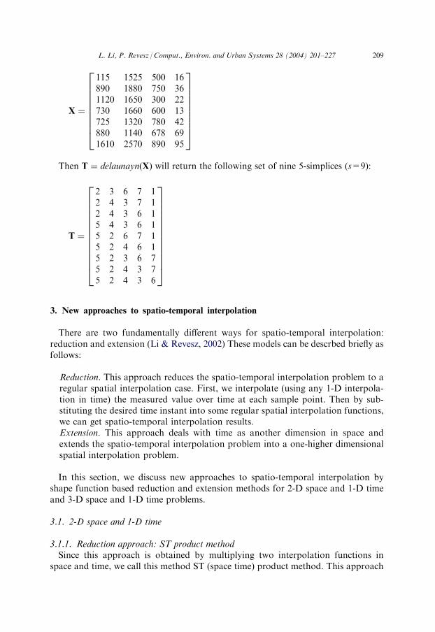
X ¼

115 1525 500 16890 1880 750 361120 1650 300 22730 1660 600 13725 1320 780 42880 1140 678 691610 2570 890 95

2666666664

3777777775

Then T ¼ delaunayn Xð Þ will return the following set of nine 5-simplices (s=9):

T ¼

2 3 6 7 12 4 3 7 12 4 3 6 15 4 3 6 15 2 6 7 15 2 4 6 15 2 3 6 75 2 4 3 75 2 4 3 6

26666666666664

37777777777775

3. New approaches to spatio-temporal interpolation

There are two fundamentally different ways for spatio-temporal interpolation:reduction and extension (Li & Revesz, 2002) These models can be descrbed briefly asfollows:

Reduction. This approach reduces the spatio-temporal interpolation problem to aregular spatial interpolation case. First, we interpolate (using any 1-D interpola-tion in time) the measured value over time at each sample point. Then by sub-stituting the desired time instant into some regular spatial interpolation functions,we can get spatio-temporal interpolation results.Extension. This approach deals with time as another dimension in space andextends the spatio-temporal interpolation problem into a one-higher dimensionalspatial interpolation problem.

In this section, we discuss new approaches to spatio-temporal interpolation byshape function based reduction and extension methods for 2-D space and 1-D timeand 3-D space and 1-D time problems.

3.1. 2-D space and 1-D time

3.1.1. Reduction approach: ST product methodSince this approach is obtained by multiplying two interpolation functions in

space and time, we call this method ST (space time) product method. This approach


for 2-D space and 1-D time problems can be described by two steps: 2-D spatialinterpolation by shape functions for triangles (Section 2.1) and approximation inspace and time (Section 3.1.1.1). Although there exists similar shape function basedST product methods such as the temperature distribution function in time-depen-dent heat conduction problems (Huebner, 1975), we discuss in this paper anST product method which combines 2-D shape function in space and 1-D shapefunction in time.

3.1.1.1. Approximation in space and time. Since in the reduction approach we modeltime independently, approximation in space and time can be implemented bycombining a time shape function with the space approximation function (1).

Assume the value at node i at time t1 is wi1, and at time t2 the value is wi2. Thevalue at the node i at any time between t1 and t2 can be approximated using a 1-Dtime shape function in the following way:

wi tð Þ ¼t2 � t

t2 � t1wi1 þ

t� t1t2 � t1

wi2: ð9Þ

Using the example shown in Fig. 1 and utilizing formulas (1) and (9), theapproximation function for any point constraint to element I at any time between t1and t2 can be expressed as follows (Li & Revesz, 2002)

w x; y; tð Þ ¼ N1 x; yð Þt2 � t

t2 � t1w11 þ

t� t1t2 � t1

w12

� �

þN2 x; yð Þt2 � t

t2 � t1w21 þ

t� t1t2 � t1

w22

� �

þN3 x; yð Þt2 � t

t2 � t1w31 þ

t� t1t2 � t1

w32

� �

¼t2 � t

t2 � t1N1 x; yð Þw11 þN2 x; yð Þw21 þN3 x; yð Þw31½ �

þt� t1t2 � t1

N1 x; yð Þw12 þN2 x; yð Þw22 þN3 x; yð Þw32½ �:

ð10Þ

Since the space shape functions (N1, N2 and N3) and the time shape functions (9)are linear, the spatio-temporal approximation function (10) is not linear butquadratic.

3.1.1.2. Visualization. The spatio-temporal interpolation result from this approachcan be visualized in a 2-D display at different time instances. We illustrate thevisualization result using a set of real estate data obtained from the Lancastercounty assessor’s office in Lincoln, Nebraska. House sale histories since 1990 arerecorded in the real estate data set and include sale prices and times. We randomlyselect 126 residential houses from a quarter of a section of a township, which coversan area of 160 acres. Furthermore, from these 126 houses, we randomly select 76(60%) houses as sample data, and the remaining 50 (40%) houses are used as test


data. Tables 1 and 2 show instances of these two data sets. Based on the fact that theearliest sale of the houses in this neighborhood is in 1990, we encode the time in sucha way that 1 represents January 1990, 2 represents February 1990, . . ., 148 representsApril 2002. Note that some houses were sold more than once in the past, so the salescorresponds to different tuples. For example, the house at the location (2215, 110)was sold at times 27, 77, and 114 (which represent 3/1992, 5/1996, and 6/1999).

For the color plot, six basic colors are chosen: red, yellow, green, turquoise, blue,and purple. The 24-bit RGB values for these colors are the following: red=(255, 0,0), yellow=(255, 255, 0), green=(0, 255, 0), turquoise=(0, 255, 255), blue=(0, 0,255), purple=(255, 0, 255). The colors are used to represent interpolated values. Thefollowing two versions of color rendering are used in the program implementation:

Version 1: Use of 400 Smoothly Changing Colors. A 1-D linear shape functioninterpolation scheme is used between each pair of the basic colors. Five simplelinear interpolations are chosen for the color changes between red and yellow,yellow and green, green and turquoise, turquoise and blue, blue and purple. Thisversion yields a smooth change of colors in the visualization, hence it avoids sharpcolor transitions. We give an example of one color interpolation later.

Example 3.1. Suppose that between red (255, 0, 0) and yellow (255, 255, 0), we use80 intermediate colors of the form (255, G, 0). Here the possible values of G can befound using the following linear function:

G ¼ 1 �x

80

� StartGValueþ

x

80

� EndGValue;

where x 2 [0, 80].In this example between red and yellow we have StartGValue=0 and End-

GValue=255. For other intervals, the values of StartGValue and EndGValue can bechanged accordingly.

Version 2: Use of six Colors. Only the six basic colors are used in the plots. Thecolor red is assigned for the smallest function value and the color purple isassigned for the largest value. Each color covers 1/6 of the total range of values for

Table 1

Sample (x,y,t,p)

X
Y T P (price/square foot)
888
115 4 56.14
888
115 76 76.02
1630
115 118 86.02
1630.
115. 123. 83.87. .. .. .. ..
2240
2380 51 91.87
2650
1190 43 63.27

the house price/square foot. This version results in visualizations that showdistinct boundaries between colors. Although this version seems to have lessinformation than the first color rendering version, for users this may be moreconvenient in categorizing house price differences. Actually, this version can beconsidered as an extreme case of the previous version with no intermediate colors.

In Figs. 6 and 7, the graphical output for the presentation of measured house pricedata is illustrated.

3.1.2. Extension approach: 3-D methodThis method treats time as a regular third dimension. Since it extends 2-D

problems to 3-D problems, this method is very similar to the linear approximationby 3-D shape functions for tetrahedra (Section 2.2). The only modification is tosubstitute variable z in Eqs. (5)–(8) by the time variable t.

3.1.2.1. Visualization. The spatio-temporal interpolation result from this approachcan be visualized in a vertical profile display. Using the same real estate data exam-ple as in Section 3.1.1, the graphical output from this extension approach is illu-strated in Fig. 8. The three slices in the figure corresponds to house pricevisualizations at three time instances: August 1991, October 1995 and December1999. They are obtained by intersecting three horizontal time planes with the tetra-hedral mesh of the 76 sample houses. Note that after tetrahedral meshing, each slicehas a different coverage of area. Fig. 8 was produced by Matlab 6.0.

3.2. 3-D space and 1-D time

In this section, we discuss the shape function based reduction and extensionapproaches for 3-D space and 1-D time spatio-temporal problems.

3.2.1. Reduction approach: ST product methodThis shape function based reduction data approximation in 3-D space and 1-D

time can be described in the following two steps: 3-D spatial interpolation by shapefunctions for tetrahedra (Section 2.2) and approximation in space and time.

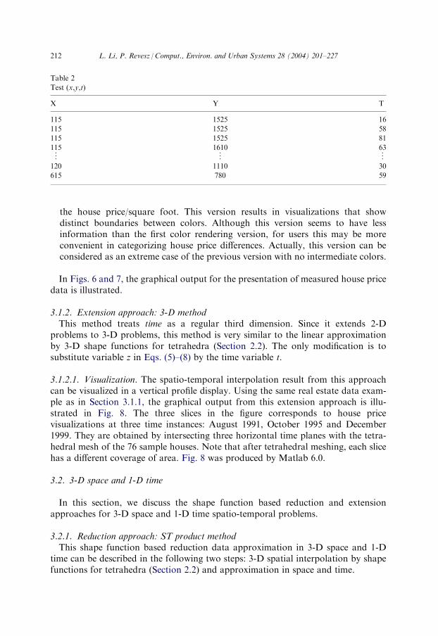
Table 2

Test (x,y,t)

X
Y T
115
1525 16
115
1525 58
115
1525 81
115.
1610. 63. .. .. ..
120
1110 30
615
780 59

Fig. 6. Version 1: continuous color rendering for the house price data of Lincoln, Nebraska in October 1995.

Fig. 7. Version 2: rendering with six discrete colors for the house price data of Lincoln, Nebraska in

October 1995.


3.2.1.1. Approximation in space and time. Similarly to the reduction approach to2-D problems, 3-D approximation in space and time can be implemented by com-bining the time shape function (9) with the space approximation function (5). Using theexample shown in Fig. 4, the linear approximation function for any point constraintto the sub-domain I at any time between t1 and t2 can be expressed as follows:

w x;ð
y; z; tÞ ¼ N1 x; y; zð Þt2 � t
t2 � t1w11 þ

t� t1t2 � t1

w12

� �

þN2 x; y; zð Þt2 � t

t2 � t1w21 þ

t� t1t2 � t1

w22

� �


t2 � t1w31 þ

t� t1t2 � t1

w32

� �


t2 � t1w41 þ

t� t1t2 � t1

w42

� �

¼ t2�t

t2�t1N1 x; y; zð Þw11 þN2 x; y; zð Þw21 þN3 x; y; zð Þw31 þN4 x; y; zð Þw41½ �

þt�t1t2�t1

N1 x; y; zð Þw12þN2 x; y; zð Þw22 þN3 x; y; zð Þw32 þN4 x; y; zð Þw42½ �:

ð11Þ

Fig. 8. Vertical profile of house price data of Lincoln, Nebraska in August 1991, October 1995 and

December 1999.


ce the space shape functions (N1, N2, N3 and N4) and the time shape functions
Sin(9) are linear, the spatio-temporal approximation function (11) is quadratic.
3.2.2. Extension approach: 4-D methodThis method treats time as a regular fourth dimension. We develop new linear 4-D

shape functions to solve this problem. In the engineering area, the highest number ofdimensions of shape functions is three because there are no higher dimensional realobjects. By developing 4-D shape functions, we will be able to interpolate an unsam-pled value at location (x,y,z) and time t. For example, the location can be houselocations, including the elevation z. In a flat city the elevation is not important. In ahilly city the elevation may be important (e.g. nice ocean view may be preferred).

Our linear 4-D shape functions are based on 4-D Delaunay tesselation, which isbriefly described in Section 2.3. In this section, we develop new 4-D shape functionsusing two different approaches. Although they yield mathematically equivalentresults, the first approach yields very long symbolic expressions whereas the secondapproach gives simple expressions.

3.2.2.1. Approach I. Since we want to develop linear 4-D shape functions to do the4-D approximation, we can assume that within each element we have someconstants a, b, c, d and e such that:


w x; y; z; tð Þ ¼ aþ bxþ cyþ dzþ et:

Let � x; y; z; tð Þ ¼ 1; x; y; z; t½ � and fT ¼ a; b; c; d; e½ �, we have

w x; y; z; tð Þ ¼ � x; y; z; tð Þf: ð12Þ

We use the five known nodal values (wis, 14i45) to calculate f as follows:

� x1; y1; z1; t1ð Þf ¼ w1

� x2; y2; z2; t2ð Þf ¼ w2

� x3; y3; z3; t3ð Þf ¼ w3

� x4; y4; z4; t4ð Þf ¼ w4

� x5; y5; z5; t5ð Þf ¼ w5

This can be written as Af=w, where

A ¼

� x1; y1; z1; t1ð Þ

� x2; y2; z2; t2ð Þ

� x3; y3; z3; t3ð Þ

� x4; y4; z4; t4ð Þ

� x5; y5; z5; t5ð Þ

266664

377775;

wT ¼ w1;w2;w3;w4;w5½ �. We obtain the solution for f as:
and
f ¼ A�1w: ð13Þ

Let

N x; y; z; tð Þ ¼ � x; y; z; tð ÞA�1: ð14Þ

After substituting (13) into (12), we have

w x; y; z; tð Þ ¼ � x; y; z; tð ÞA�1w

¼ N x; y; z; tð Þw

¼ N1N2N3N4N5½ �

w1

w2

w3

w4

w5

26666664

37777775

ð15Þ

Now it is clear that (14) is the shape and function matrix that we need to find. Wecalculated the result of (14) by Matlab. Since A is a 55 matrix in symbolic form, itsinverse is very complicated and messy. The expression result of N based on the xis,yis, zis, tis and wis (14i45) is very redundant and unreadable. Each shape functionexpression Ni (14i45) covers about four pages. Next, we introduce a secondapproach which is based on the linear 3-D shape functions (6) or (8) and yields aneat symbolic expression.

3.2.2.2. Approach II. The idea in the second approach is to reduce the 4-D case to a3-D case. This can be done if the deletion of a dimension does not collapse twonodes into one. For example, if we have (x,y,z,t) data points and we delete z coor-dinates, then we should not get two points with the same (x,y,t) values. Let usdenote the 3-D shape functions by Ni (x,y,z) (14i44). Then the 4-D linearapproximation in terms of these can be expressed as follows:

w x; y; z; tð Þ ¼ aN1 x; y; zð Þ þ bN2 x; y; zð Þ þ cN3 x; y; zð Þ þ dN4 x; y; zð Þ þ et:

h i
Let � x; y; z; tð Þ ¼ N1 x; y; zð Þ; N2 x; y; zð Þ; N3 x; y; zð Þ; N4 x; y; zð Þ; t and
fT ¼ a; b; c; d; eh i

, we have:

w x; y; z; tð Þ ¼ � x; y; z; tð Þf: ð16Þ

We use the five known nodal values (wis, 14i45) to calculate f as follows:

� x1; y1; z1; t1ð Þf ¼ w1

� x2; y2; z2; t2ð Þf ¼ w3


� x3; y3; z3; t3ð Þf ¼ w3

� x4; y4; z4; t4ð Þf ¼ w4

� x5; y5; z5; t5ð Þf ¼ w5

Assuming mi ¼ Ni x5; y5; z5ð Þ 14 i4 4ð Þ, this can be written as Bf ¼ w, where

B ¼

� x1; y1; z1; t1ð Þ

� x2; y2; z2; t2ð Þ

� x3; y3; z3; t3ð Þ

� x4; y4; z4; t4ð Þ

� x5; y5; z5; t5ð Þ

266664

377775 ¼

1 0 0 0 t10 1 0 0 t20 0 1 0 t30 0 0 1 t4m1 m2 m3 m4 t5

266664

377775

and wT ¼ w1;w2;w3;w4;w5½ �.We obtain the solution for f as:

f ¼ B�1w: ð17Þ

Let

N x; y; z; tð Þ ¼ � x; y; z; tð ÞB�1: ð18Þ

After substituting (17) into (16), we have

w x; y; z; tð Þ ¼ � x; y; z; tð ÞB�1w

¼ N x; y; z; tð Þw

¼ N1N2N3N4N5½ �

w1

w2

w3

w4

w5

26666664

37777775

ð19Þ

The shape function result of (18) can be calculated as follows:

Ni ¼ Ni þmih

detB14 i4 4ð Þ and N5 ¼

h

detB; ð20Þ

where detB ¼ �m1t1 �m2t2 �m3t3 �m4t4 þ t5 is the determinant of B andh ¼ N1t1 þ N2t2 þ N3t3 þ N4t4 � t. This method can be generalized to derive shapefunctions of n dimension from shape functions of n�1 dimensions.

4. Comparison with IDW and kriging for 2-D space and 1-D time problems

So far we have discussed the reduction and extension approaches for the shapefunction based interpolation methods. Other spatial interpolation methods may also


have reduction and extension approaches for spatio-temporal problems. In thissection, based on the same set of actual real estate data as used in Sections 3.1.1 and3.1.2, we will compare the above shape function based methods with inversedistance weighting (IDW) and kriging interpolation methods in both reduction andextension approaches.

4.1. Experimental result of shape function based methods

4.1.1. AccuracyWe compare the estimated values of price per square foot with the true values

for each sale instance of the 50 test houses according to MAE and RMSE. Thedefinition of MAE and RMSE is as follows:

MAE ¼

PNi¼1

Ii �Oij j

NRMSE ¼

ffiffiffiffiffiffiffiffiffiffiffiffiffiffiffiffiffiffiffiffiffiffiffiffiPNi¼1

Ii �Oið Þ2

N

vuuut

where N is the number of test houses, Ii is the interpolated house price, and Oi is theoriginal house price.

In Table 3, the MAE and RMSE columns summarize the accuracy analysis of themethods. We can see that the ST product method yields a slightly better accuracy(less MAE and RMSE values) than the 3-D method for shape function based inter-polation.

4.1.2. Error-proneness to time aggregationThe unit of time is a special issue for spatio-temporal data. For example, the

following questions are of interest:

(1) For a specific spatio-temporal data set, how fine should the granularity of timebe to obtain the best result of interpolation?(2) For some data sets that only have a coarse granularity of time, what kind ofspatio-temporal interpolation methods should be used?

To answer these questions, the error criteria of MAE and RMSE have beenmeasured according to twelve different ways of time aggregation of the house pricedata. The twelve approaches of time aggregation include monthly, bimonthly,quarterly, . . ., yearly. That is, each month is treated as a different time instance inmonthly aggregation, every two months are treated a different time instance inbimonthly aggregation, . . ., each year is treated as a different time instance in yearlyaggregation.

Fig. 9 shows the experimental results of RMSE for error proneness to timeaggregation of the shape function based methods. The results of MAE are verysimilar to RMSE. The Matlab function polyfit has been used to calculate the linearregression functions. In Table 3, the column Slope summarizes the slopes of MAEand RMSE linear regression functions. Steeper slope indicates less error-proneness


to time aggregation. It is shown that the 3-D method is much less error-prone thanthe ST product method.

4.1.3. Constraint typesFor the ST product method, if wis (14i43) are linear functions of t, the

constraint types are quadratic; if we use a polynomial function of t to approximatethe wis, we will get even higher polynomial functions for wis. For the 3-D method,

Table 3

Comparison results

Method
MAE RMSE Slope Constraint Invariance
MAE
RMSE
Reduction (ST Product)
Shape Func 8.98 11.34 9.69 13.08 Polynomial Yes
IDW (n=3, P=1)
10.05 11.96 9.49 13.62 Polynomial No
Shape Func
7.92 10.11 0.34 0.69 Linear Yes
Extension (3-D)
IDW (n=3, P=1) 11.14 13.63 0.06 0.07 Polynomial No
Kriging
10.25 12.59 0.07 0.08 Polynomial No
Fig. 9. Shape function susceptibility to time aggregation according to root mean square error (RMSE).

The solid lines are the actual result, while the dashed lines are the linear regression functions that best

approximate the tendency of RMSE.


we can find in linear time a constraint relation to represent the whole interpolationby representing the tetrahedral method in each tetrahedron with a separateconstraint tuple (Li & Revesz, 2002).

In Table 3, the Constraint Type column summarizes the type of constraints of thesemethods. For shape function based approaches, since the 3-D method yields onlylinear constraints and the ST product yields polynomial constraints, the 3-D methodhas an advantage over the ST product method: query evaluation is more efficient.

4.1.4. Invariance to coordinate scalingShape functions for triangles and tetrahedra are invariant to coordinate scaling,

which means their results will remain the same even if the scale of a dimension (ordimensions) changes. Being invariance to coordinate scale is a very charming char-acteristic of a spatio-temporal interpolation method especially when we want to usethe extension approach. This is because we do not have to worry about what time unitshould be used when mixing the space and time dimension. In Table 3, the columnInvariance summarizes whether the method is invariant to coordinate scaling. We provethat 2-D triangular shape functions are invariant to scaling in below. The proof for theinvariance of 3-D tetrahedral shape functions can be similarly obtained.

Proof 4.1. 2-D triangular shape functions are invariance to coordinate scaling.Consider N1(x,y) in the triangular shape function (2). After substituting the

determinant result of A, we have


x2y3 � y2x3 � x1y3 þ y1x3 þ x1y2 � y1x2:

Assume that the scale in x dimension enlarges to n times of the original scale.Then N1 will be as follows after scaling

N0

1x; yð Þ ¼

nx2y3 � nx3y2ð Þ þ nx y2 � y3ð Þ þ y nx3 � nx2ð Þ½ �

nx2y3 � ny2x3 � nx1y3 þ ny1x3 þ nx1y2 � ny1x2;

which is obviously the same result as before scaling. Invariance to y scale isstraightforward too. Similarly, we can prove that N2 and N3 are also invariant tocoordinate scaling. &

4.2. Experimental result of IDW-based methods

IDW interpolation is based on the assumption that things that are close to oneanother are more alike than those that are farther apart. Revesz and Li (2002a) usesIDW to visualize spatial interpolation data. In IDW, the measured values (knownvalues) closer to prediction location will have more influence on the predicted value(unknown value) than those farther away. More specifically, IDW assumes that eachmeasured point has a local influence that diminishes distance. Thus, points in the


near neighbourhood are given high weights, whereas points at a far distance aregiven small weights.

According to Johnston, Hoef, Krivoruchko, and Lucas (2001), the general formulaof IDW interpolation is the following:

w x; yð Þ ¼PNi¼1

liwi; li ¼

1

di

� �p

PNk¼1

1

dk

� �p ; ð21Þ

where w(x,y) is the predicted value at location (x,y), N is the number of nearestknown points surrounding (x,y), li are the weights assigned to each known pointvalue wi at location (xi,yi), di are the Euclidean distances between each (xi,yi) and(x,y), and p is the exponent, which influences the weighting of wi on w.

Since the experimental data is 2-D, next we briefly discuss the IDW based reductionand extension approaches to 2-D problem. For 3-D problem, the formulae can besimilarly derived.Reduction Approach. Assume we are interested in the value of the unsampled point

at location (x,y) and time t. This approach first finds the nearest neighbors of foreach unsampled point and calculates the corresponding weights li. Then, it calcu-lates for each neighbor the value at time t by some time interpolation method. If weuse shape function interpolation in time, the time interpolation will be similar to (9).The formula of this approach can be expressed as:

w x; y; tð Þ ¼PNi¼1

liwi tð Þ; li ¼

1

di

� �p

PNk¼1

1

dk

� �p ð22Þ

where

wi tð Þ ¼ti2 � t

ti2 � ti1wi1 þ

t� ti1ti2 � ti1

wi2: ð23Þ

Each neighbor may have different beginning and ending times ti1 and ti2 in (23) ifeach point is sampled at different times.Extension Approach Since this method treats time as a third dimension, the

IDW based spatio-temporal formula is of the form of (21) with

di ¼

ffiffiffiffiffiffiffiffiffiffiffiffiffiffiffiffiffiffiffiffiffiffiffiffiffiffiffiffiffiffiffiffiffiffiffiffiffiffiffiffiffiffiffiffiffiffiffiffiffiffiffiffiffiffiffiffiffixi � xð Þ

2þ yi � yð Þ

2þ ti � tð Þ

2q

.

4.2.1. AccuracyFrom the MAE and RMSE columns in Table 3, we can see that as different

from the shape function based methods, the 3-D method yields a slightly betteraccuracy (less MAE and RMSE values) than the ST product method for IDW-based interpolation.


4.2.2. Error-proneness to time aggregationSimilarly to the analysis of shape function-based methods, we test the same 12

ways of time aggregation for the IDW-based methods. Fig. 10 show the experi-mental results of RMSE for error proneness to time aggregation of the IDW basedmethods when the number of near neighbors is 3. The results of MAE are verysimilar to RMSE. From the column Slope in Table 3, we can see that similarly to theshape function-based methods, the 3-D method is much less error-prone than the STproduct method for IDW-based approaches.

4.2.3. Constraint typesThe constraint type for both the IDW-based ST product and 3-D methods are

polynomial.

4.2.4. Non-invariance to coordinate scalingIDW is not invariance to coordinate scaling. Consider the IDW interpolation with

2 neighbors and power 2, based on Eq. (21), we have

l1 ¼x� x2ð Þ

2þ y� y2ð Þ

2

x� x1ð Þ2þ y� y1ð Þ

2þ x� x2ð Þ

2þ y� y2ð Þ

2:

Fig. 10. IDW susceptibility to time aggregation according to root mean square error (RMSE). The solid

lines are the actual result, while the dashed lines are the linear regression functions that best approximate

the tendency of RMSE.


Assume that the x dimensional scale enlarges to n times. Then after scaling, l1 willbe

l01 ¼n2 x� x2ð Þ

2þ y� y2ð Þ

2

n2 x� x1ð Þ2þ y� y1ð Þ

2þn2 x� x2ð Þ

2þ y� y2ð Þ

2;

which is not the same result as before scaling. Therefore, IDW is not invariant tocoordinate scaling.

4.3. Experimental result of kriging-based methods

Kriging is an important interpolation method by using geostatistical analysiswhich provides a minimum error-variance estimate of any unsampled value. It wasinitially introduced by D.G. Krige as an optimal interpolation method in the miningindustry (Krige, 1951). It was later developed by G. Matheron as the theory ofregionalized variables (Matheron, 1971). Using kriging as an interpolation method inGIS was discussed by Oliver and Webster (1990).

Kriging is similar to IDW in the sense that it uses a weighting mechanism thatassigns more influence to the nearer data points to interpolate values at unknownlocations. However, instead of using inverse distance weighting approach, kriginguses variograms. As a measure of spatial variability, a variogram replaces theEuclidean distance by a structural distance that is specific to the attribute and thefield under study (Deutsch & Journel, 1998). Assume u is a location vector where thedata value is unsampled. The variogram distance measures the average degree ofdissimilarity between w(u) and a nearby known data value. For example, given twosampled data values w1 and w2 at two different locations u+h1 and u+h2, the more‘‘dissimilar’’ sample value should receive less weight in the estimation of w(u).Reduction Approach. This is not a feasible approach for kriging. According to

Lam (1983), a variogram (2r) can be defined as

2r ¼1

N

XNi¼1

w ui þ hð Þ � w uið Þ½ �2

ð24Þ

where h is the distance between two samples and N is the number of pairs of sampleshaving the same distance.

From Eq. (24), we can see that not only do variograms depend on the locationdistribution (h) of samples, but also depend on the sample values (w). Since weightsare determined by variograms, weights are also both location and informationdependent. That is, weights can not be calculated without knowing the values ofsample points. So, if we want to use reduction approach, we have to know inadvance which sampled points will be used in kriging for each unsampled points andthen use some temporal interpolation method to estimate the sample values at thetime the unsampled point is interested in. However, different unknown points mayshare some same sample points. This leads to the ambiguity about the values at what


time shall be used for those sample points. Therefore, the reduction approach ofspatio-temporal interpolation is not feasible for kriging.Extension Approach. Since kriging can be generalized into high dimension, the

extension approach of kriging is a natural approach for spatio-temporal interpola-tion. There are multiple types of kriging, such as simple kriging, ordinary kriging,universal kriging, and factorial kriging. Because ordinary kriging is the most com-monly used variant of simple kriging and it has been the anchor algorithm of geo-statistics (Deutsch & journel, 1998), we choose 3-D ordinary kriging to interpolatethe house experimental data. By ordinary kriging, the estimation for unknownlocation u is calculated as:

w uð Þ ¼PNi¼1

liwi;PNi¼1

li ¼ 1 ; ð25Þ

where weights li are determined by variograms to minimize the error variance.We use the Matlab Kriging Toolbox (version 4.0) provided by Gratton to do the

experiments. It is available from http://www.inrs-eau.uquebec.ca/activites/reper-toire/yves_gratton/krig.htm. This toolbox is almost entirely made up of functionsfrom Deutsch and Journel (1998) and Marcotte (1991). It actually implemented highdimensional cokriging with Matlab. Cokriging is the multi-variable extension ofkriging. It means kriging with more than one variables. When the cokriging pro-gram is called with only one variable, it will return the kriging result. Since we haveonly one variable, the house price, we only need kriging.

4.3.1. AccuracyWith the search radius being 500, the number of nearest neighbors will be 10, and

some other default input parameters for point cokriging, we have tested severalchoices of variogram models. The result of linear model with nugget effect has beenthe best. We put the result of this model into Table 3. The MAE and RMSE valuesof kriging based 3-D method are slightly better than the IDW-based 3-D method.But they are worse than shape function-based both ST product and 3-D methods.

4.3.2. Error-proneness to time aggregationSimilarly to the analysis of shape function and IDW-based methods, we test the

same 12 ways of time aggregation for the kriging based 3-D method. Fig. 11 showsthe experimental results of both MAE and RMSE. From the column Slope inTable 3, we can see that the kriging based 3-D method is not error-prone.

4.3.3. Constraint typesThe constraint type for the kriging-based 3-D method is polynomial since the

calculation of variograms by Eq. (24) is already quadratic.

4.3.4. Non-invariance to coordinate scalingSince kriging is similar to IDW in the weighting mechanism that is influenced by

distances, kriging is also not invariant to coordinate scaling.


5. 4-D Shape function example for 3-D space and 1-D time problems

We implemented the 4-D shape functions in Section 3.2.2 by Matlab. We alsoextended the 2-D space and 1-D time real estate example to a 3-D space and 1-Dtime problem by adding the elevation information to each house as shown inTables 4 and 5.

We used our Matlab program to interpolate the 4-D test data and compared itwith the original values according to MAE and RMSE. The result of MAE is 8.54and the result of RMSE is 10.25. These results are slightly worse than the 3-D shapefunctions methods in Table 3. This can be explained by the fact that the elevations

Fig. 11. Kriging susceptibility to time aggregation according to mean absolute error (MAE) and root

mean square error (RMSE). The solid lines are the actual result of MAE and RMSE, while the dashed

lines are the linear regression functions that best approximate their tendency.

Table 4

Sample 4-D (x,y,z,t,p)

X
Y Z T P (price/square foot)
888
115 1305 4 56.14
888
115 1305 76 76.02
1630
115 1294 118 86.02
1630.
115. 1294. 123. 83.87. .. .. .. .. ..
2240
2380 1295 51 91.87
2650
1190 1288 43 63.27

of those houses in the selected test area are similar and the house elevation is not afactor to contribute to house prices. Therefore, it adds noise to the interpolation byconsidering the house elevation.

6. Future work

For the extension method based on shape functions the resulting spatio-temporalinterpolation data can be represented using linear equality and inequality con-straints. While there are many ways of storing this representation, constraint data-bases (Kanellakis, Kuper, & Revesz 1995; Kuper, Libkin, & Paredaens, 2000;Revesz, 2002) are a convenient alternative. Linear constraint databases used in theDEDALE system (Grumbach, Rigaux, & Segoufin, 2000) and the MLPQ system—see Chapter 18 in (Revesz, 2002)—are particularly natural for this type of inter-polated data. The advantages of using MLPQ include compact data storage, con-venient database querying, and the availability of a number of built-in visualizationtools, including some for spatio-temporal animation. For future work, we plan touse this representation for the real estate data set and also experiment with otherdata sets.

Acknowledgements

The authors would like to thank Professor Reinhard Piltner for the discussion ofshape functions and finite elements.

References

Buchanan, G. R. (1995). Finite element analysis. New York: McGraw-Hill.

Deutsch, C. V., & Journel, A. G. (1998). GSLIB: geostatistical software library and user’s guide (2nd ed.).

New York: Oxford University Press.

Freitag, L. A., & Gooch, C. O. (1997). Tetrahedral mesh improvement using swapping and smoothing.

International Journal for Numerical Methods in Engineering, 40, 3979–4002.

Table 5

Test 4-D (x,y,z,t)

X
Y Z T
115
1525 1294 16
115
1525 1294 58
115
1525 1294 81
115.
1610. 1293. 63. .. .. .. ..
120
1110 1300 30
615
780 1306 59

Goodman, J. E., & O’Rourke, J. (Eds.). (1997). Handbook of discrete and computational geometry. Boca

Raton, NY: CRC Press.

Grumbach, S., Rigaux, P., & Segoufin, L. (2000). Manipulating interpolated data is easier than you

thought. In Proc. of IEEE International Conference on very large databases (pp. 156–165).

Harbaugh, J. W., & Preston, F. W. (1968). Fourier analysis in geology. Englewood Cliffs: Prentice-Hall.

Huebner, K. H. (1975). The finite element method for engineers. New York: John Wiley and Sons.

Johnston, K., Hoef, J. M. V., Krivoruchko, K., & Lucas, N. (2001). Using ArcGIS geostatistical analyst.

ESRI Press.

Kanellakis, P. C., Kuper, G. M., & Revesz, P. (1995). Constraint query languages. Journal of Computer

and System Sciences, 51(1), 26–52.

Krige, D. G. (1951). A statistical approach to some mine valuations and allied problems at the witwaters-

rand. Master’s thesis, University of Witwatersrand, South Africa.

Kuper, G. M., Libkin, L., & Paredaens, J. (Eds.) (2000). Constraint databases. Springer-Verlag.

Lam, N. S. (1983). Spatial interpolation methods: a review. The American Cartographer, 10(2), 129–149.

Li, L., & Revesz, P. (2002). A comparison of spatio-temporal interpolation methods. In M. Egenhofer, &

D. Mark (Eds.), Proc. of the Second International Conference on GIScience 2002 (Vol. 2478 of Lecture

Notes in Computer Science, pp. 145–160). Springer-Verlag.

Marcotte, D. (1991). Cokriging with Matlab. Computer & Geosciences, 17(9), 1265–1280.

Matheron, G. (1971). The theory of regionalized variables and its applications. Les Cahiers du Centre de

Morphologie Mathematique de Fontainebleau, 5.

Miller, E. J. (1997). Towards a 4D GIS: four-dimensional interpolation utilizing kriging. In Z. Kemp

(Ed.), Innovations in GIS 4: selected papers from the Fourth National Conference on GIS Research UK

(pp. 181–197). London: Taylor & Francis.

Oliver, M. A., & Webster, R. (1990). Kriging: a method of interpolation for geographical information

systems. International Journal of Geographical Information Systems, 4(3), 313–332.

Preparata, F. P., & Shamos, M. I. (1985). Computational geometry: an introduction. Springer-Verlag.

Revesz, P. (2002). Introduction to constraint databases. Springer-Verlag.

Revesz, P., & Li, L. (2002a). Constraint-based visualization of spatial interpolation data. In Proc. of the

Sixth International Conference on information visualization (pp. 563–569). London, England: IEEE

Press.

Revesz, P., & Li, L. (2002b). Representation and querying of interpolation data in constraint databases.

In Proc. of the Second National Conference on digital government research (pp. 225–228). Los Angeles,

CA.

Shepard, D. (1968). A two-dimensional interpolation function for irregularly spaced data. In Proc. 23nd

National Conference ACM (pp. 517–524). ACM.

Shewchuk, J. R. (1996). Triangle: engineering a 2D quality mesh generator and delaunay triangulator. In

Proc. First Workshop on applied computational geometry (pp. 124–133). Philadelphia, PA.

Shewchuk, J. R. (1998). Tetrahedral mesh generation by delaunay refinement. In Proc. 14th Annual ACM

Symposium on computational geometry (pp. 86–95). Minneapolis, MN.

Watson, D. F. (1981). Computing the n-dimensional delaunay tesselation with application to voronoi

polytopes. The Computer Journal, 24(2), 167–172.

Zienkiewics, O. C., & Taylor, R. L. (1989). Finite element method. In The basic formulation and linear

problems (Vol. 1). McGraw-Hill.

Zienkiewics, O. C., & Taylor, R. L. (2000). Finite element method. In The basis (Vol. 1). London:

Butterworth Heinemann.

Zurflueh, E. G. (1967). Applications of two-dimensional linear wavelength filtering. Geophysics, 32, 1015–

1035.


Documents

Interpolation methods for spatio-temporal geographic data