International Journal of Pure and Applied Mathematics · ume deformation, tensor product, computer-aided geometri c design, spline, B-spline ... (an a ne mapping) of the BFBS basis

International Journal of Pure and Applied Mathematics————————————————————————–Volume 65 No. 3 2010, 339-360

GEOMETRIC MODELLING

WITH BETA-FUNCTION B-SPLINES, I:

PARAMETRIC CURVES

Arne Laksa1, Børre Bang2, Lubomir T. Dechevsky3 §

1,2,3R&D Group for Mathematical Modelling,Numerical Simulation and Computer Visualization

Faculty of TechnologyNarvik University College

2, Lodve Lange’s Str., P.O. Box 385, N-8505, Narvik, NORWAY1e-mail: [email protected]

url: http://ansatte.hin.no/ala/2e-mail: [email protected]

url: http://ansatte.hin.no/bb/3e-mail: [email protected]

url: http://ansatte.hin.no/ltd/

Abstract: This is the first one in a sequence of several papers dedicated tothe development of applications of Euler Beta-function B-splines (BFBS) toComputer-aided Geometric Design (CAGD) and, in particular, for geometricmodelling of parametric curves, surfaces and volume deformations. This studyis an analogue of the study conducted in [12, 10] for the case of expo-rational B-splines (ERBS). An important objective of this study is the comparison betweenthe graphical and computational performance of BFBS versus ERBS, as wellas the comparison of BFBS versus classical polynomial Schoenberg B-splines.

In the present paper we discuss parametric curve interpolation based onBFBS, as well as the respective Bezier-type curve representation.

AMS Subject Classification: 53A04, 65D05, 65D07, 65D17, 26A63, 26B15,28A75, 33B15, 33B20, 33F05, 41A15, 41A30, 42A38, 44A10, 50A30, 51M25,52A38, 53A05, 53A15, 53A17, 53A20, 65D10, 65D20, 65D30

Received: March 2, 2010 c© 2010 Academic Publications§Correspondence author

340 A. Laksa, B. Bang, L.T. Dechevsky

Key Words: geometric modelling, parametrization, curve, surface, vol-ume deformation, tensor product, computer-aided geometric design, spline,B-spline, polynomial, exponential, rational, expo-rational, generalized, EulerBeta-function, complete, incomplete, Gamma-function, scalar, vector, point,matrix, piecewise, linear, affine, barycentric, convex, continuous, differentiable,smooth, Hermite interpolation, monomial basis, Bernstein basis, Bezier curve,control polygon, de Casteljau algorithm, Cox-de Boor algorithm, iterative, lo-cal, global, constant, variable, functional

1. Introduction

Expo-rational B-splines (ERBS) were introduced in 2003, and a first compre-hensive study of their properties was conducted and announced in [1], and pub-lished in [8]; their applications to geometric modelling of curves and surfaceswere first studied in [12] and, in considerable detail, in [10].

Generalized expo-rational B-splines (GERBS), first proposed in [2], withsubsequent publication in [7], are a generalization of ERBS which includes thepolynomial simplified modifications of ERBS, introduced in [2] as Euler Beta-function B-splines (BFBS), with a brief outline of their definition in [7] anda detailed exposition of their definition and properties in [3] and discussion oftheir evaluation in [4, 5, 6]. The GERBS class also includes other basis/blendingfunctions with relevant properties such as minimal support (as a 1st-degreepiecewise-affine B-spline), value 1 at the center knot, value zero at all otherknots, and (at least one) derivative equal zero at all knots.

BFBS were introduced in [2] as a particularly important practical instanceof GERBS which is essentially complementary to ERBS. In this framework, thedefinition and properties of BFBS [3] are similar to those of ERBS but theseuseful properties of BFBS [3] are only available within a limited range, com-pared to the practically unlimited range of validity of the respective propertiesof ERBS [8]. On the other hand, unlike ERBS, whose evaluation requires nu-merical integration, BFBS are explicitly and efficiently computable in closedform, in terms of polynomial bases [4, 5, 6].

Definition 1. (BFBS – see [3, Definition 4].) Consider a strictly increasingknot-vector {tk}

n+1k=0 . A Beta-function B-spline (BFBS), associated with three

strictly increasing adjacent knots tk−1, tk and tk+1, Bk(t) = Bk(ik−1, ik, ik+1; t)

GEOMETRIC MODELLING... 341

is defined by

Bk(t) =

Sk−1

t∫

tk−1

ψk−1(s)ds, if t ∈ (tk−1, tk),

Sk

tk+1∫

t

ψk(s)ds, if t ∈ (tk, tk+1),

1, if t = tk,

0, otherwise,

(1)

with

Sk =

tk+1∫

tk

ψk(t)dt

−1

, (2)

and

ψk(t) = Ck

(t− tk)ik(tk+1 − t)ik+1

(tk+1 − tk)ik+ik+1, t ∈ [tk, tk+1], (3)

where

Ck =

(ik + ik+1

ik

), (4)

and

il > 0, l = k − 1, k, k + 1. (5)

In a sequence of several papers, of which this is the first one, we studyapplications of the new BFBS to Computer-aided Geometric Design (CAGD)and, in particular, for geometric modelling of parametric curves, surfaces andvolume deformations. This study is an analogue of the study conducted in [12,10] for the case of ERBS. An important objective of this study is the comparisonbetween the graphical and computational performance of BFBS versus ERBS,as well as of BFBS versus classical polynomial Schoenberg B-splines. In thepresent paper we discuss BFBS-based parametric curve interpolation and therespective BFBS-based Bezier-type curve representation. The structure of thepaper is, as follows.

The first part of the exposition is focused on functional (scalar-valued)curves in 2D, and the second part – on parametric (vector-valued or point-valued) curves in 3D.


In Section 2.1 we define a general BFBS-based function as a linear combi-nation of Beta-function B-splines, with coefficients which may be functions, notnecessarily constants. (Here the values of the functions can be scalars (reals),vectors, or points.) These “coefficient functions” are called “local functions” or”functional coefficients”.

In Section 2.2 we discuss the multiplicities in a knot vector and the regular-ity properties of a compound spline function which these multiplicities generate.The Hermite interpolation property of fitting the “global” function to the “lo-cal” functions in the knots is investigated and discussed in Section 2.3. A shortrecipe of how to compute a BFBS function interpolating a known function isgiven.

Section 3 is an introduction to the topic of parametric curves in 3D.In Section 4 we comment on the definition and implementation of “open/

closed” curves.In Section 5, the BFBS curve evaluation, including derivatives, is discussed.In Section 6, Bezier curves are investigated as local curves, including Her-

mite interpolation in Bezier form.

2. Functional Curves in 2D

2.1. Beta-Function B-Spline Functions

One of the reasons for developing the BFBS is to use them as easily computablebasis functions (blending functions) in a compound function, as is usual withpolynomial B-spline functions. In a classical polynomial B-spline function be-tween two adjacent knots, there is a polynomial of degree d composed by abarycentric combination of d + 1 coefficients, weighted by d+ 1 B-spline basisfunctions. In a BFBS function there are, inside one knot segment, only 2 basisfunctions that are different from zero.

First, we shall consider the case when all coefficients in the linear combina-tion of the BFBS are constants (scalars, vectors or points):

f(t) =n∑

i=1

ciBi(t), t ∈ [t1, tn]

According to [3, Theorem 1], every BFBS is interpolating ’its’ functionalcoefficient at ’its’ knot, while being zero at each other knot. In each segment(between two adjacent knots), a scalar BFBS function will be a scaled andtranslated version (an affine mapping) of the BFBS basis function. It will


Figure 1: An approximate global BFBS function f(t) (blue) with fourscalar coefficients {ci}

4i=1 (green). The global function is a blending of

the coefficients, with the Beta-function B-splines {Bi(t)}4i=1 (red) being

the blending functions. The global function interpolates the coefficients,and all derivatives are zero at all knots. The knot vector {ti}

5i=0 is

also marked, and there are multiple knots at both ends (discontinuityis discussed in Section 2.2). In a greyscale version of the image, allcolours used range within different ranges of the greyscale value.

interpolate the coefficients, and the derivatives will have zero values where theBFBS basis function has a zero-value derivative. This behavior is illustrated inFigure 1. We will have the following inside a knot interval:

f(t) = ci Bi(t) + ci+1 Bi+1(t), if ti < t < ti+1. (6)

From property Q3 in [3, Theorem 1], it follows that (6) can be reformulated to

f(t) = ci+1 + (ci − ci+1)Bi(t), if ti < t < ti+1. (7)

Second, we shall consider the general case of non-constant (scalars, vectorsor points) local functions as coefficients (illustrated in Figure 2). The domainof these functions has to be the same as (or larger than) the support of therespective BFBS basis function. It means that the local function with indexk is defined (and usually bounded) on the domain (tk−1, tk+1). A practicalsolution is to map the domains from the basis functions to the local functions(see Definition 4 later in this section). Now, there follows a definition of a set offunction spaces, which is, in some sense, a constrained analogue of the definition


of local functions in the case of ERBS [8], and is a specialized version of thegeneral case of GERBS [7].

Definition 2. To characterize local functions lk(t), we define a set offunction spaces,

F(Bk) = {l : Dj(l(t)Bk(t)) = 0 for j = 0, 1, . . . , ik−1 and t = tk−1,

or j = 0, 1, . . . , ik+1 and t = tk+1,

and l is a polynomial function},

where the Bk, k = 1, . . . , n are defined in Definition 1.

Remark 1. It is possible to consider also local functions l other thanpolynomials (which still satisfy Dj(l(t)Bk(t)) = 0 for the mentioned j), buthere we consider only the polynomial case, because then the BFBS functionwill be piecewise polynomial itself, like in the classical Schoenberg B-splinecase.

Now the definition of a BFBS function follows.

Definition 3. A Beta-function B-spline (BFBS) function f(t) (scalar orvector-valued or point-valued) is defined on the domain (t1, tn] by

f(t) =

n∑

k=1

lk(t)Bk(t) if t1 < t ≤ tn,

where lk(t) are local (scalar or vector-valued or point-valued) functions definedon (tk−1, tk+1), k = 1, . . . , n, and Bk(t), k = 1, . . . , n, is defined in Definition1. It is assumed that lk(t) ∈ F(Bk).

Just like usual polynomial B-spline functions, BFBS functions (i) have basisfunctions defined by a knot vector, and (ii) form a convex partition of unity(which also means that they are invariant under affine transformations). Inaddition, the basis functions have minimal local support (the same as 1st degreeB-splines); for the typical case of simple knots tk < tk+1 properties Q1, Q3,Q4 and Q5 in [3, Theorem 1], together with lk(t) ∈ F(Bk), imply Hermiteinterpolation (discussed in Section 2.3). Figure 2 illustrates this clearly. Inevery knot the global function interpolates the local functions, not only thefunctional value, but also the derivatives up to order ik. The figure also showsthat the global function passes through all intersections between two neighboringlocal functions. This is because the global function is an affine combination oftwo and only two local functions for every value of the argument.


Figure 2: An approximate global BFBS function f(t) (blue) with fourlocal functions {li(t)}

4i=1 (green). The global function is a blending of

its local functions, with the BFBS {Bi(t)}4i=1 (red) being the blending

functions. The global function also completely interpolates all existingderivatives of each of the adjacent local functions at the respective knottk, up to the multiplicity ik. The knot vector {ti}

5i=0 is also marked,

and there are multiple knots at both ends (discontinuity is discussed inSection 2.2). In a greyscale version of the image, all colours used rangewithin different ranges of the greyscale value.

Using local functions offers a new possibility (or challenge, in practical im-plementation), namely, a domain mapping from segments in the “global” do-main onto the “local” domains. It, therefore, follows that local functions mustbe split up into a function on the local domain and what we define to be theaffine global/local mapping.

Definition 4. We denote the local domain for the local function lk to be,

Ik = (sk0, sk1) ⊂ R where sk0 < sk1,

and where sk0 is the start parameter value, end sk1 is the end parameter valueof the local function lk. The global/local mapping ωk is said to be the mappingof a segment (tk−1, tk+1) in the global domain of the BFBS function onto thedomain Ik,

ωk : (tk−1, tk+1) ⊂ R → Ik.


ωk is, therefore, the affine mapping

ωk(t) = sk0 +t− tk−1

tk+1 − tk−1(sk1 − sk0). (8)

The inverse mapping from Ik to (tk−1, tk+1) is

ω−1k (s) = tk−1 +

s− sk0

sk1 − sk0(tk+1 − tk−1). (9)

The possibilities in constructing a great diversity of functions depending onthe variety of local functions gives BFBS a new “dimension”, because by thisone can customize the typical properties of the function. Some brief examplesare that one can use trigonometric functions or circular arcs (in R

2 or R3),

Bezier functions, rational functions, special functions etc. The local functioncan even be a BFBS function itself, raising the possibilities for multilevel BFBS.There is nothing which says that all local functions must be of the same type.

2.2. Knot Vectors and Continuity

Multiplicity of the knots is an important issue for ERBS as well as for BFBS.In the case of ERBS, coincidence of two subsequent knots leads to discontinuityin the single knot into which the two adjacent knots have coalesced (see [10,Theorem 2.3], and, in most general form, [7]) and for BFBS the argument isexactly the same. We, therefore, do not consider this case in detail here.

2.3. Hermite Interpolation Properties

Here we study the BFBS-analogue of the Hermite interpolation properties ofERBS. We shall see that for the local functions, lk(t) ∈ F(Bk) holds, BFBSfunctions have an Hermite interpolation property; we also discuss how this canbe used. The important underlying fact here is that

DjBk(tk) = 0, if k = 1, ..., n and j = 1, 2, ..., ik

which is property Q4((d1).1) in [3, Theorem 1]. Let us now increase the gen-eralization to a higher dimensional value of the function,

f : (t1, tn] → Rd, where 1 ≤ d <∞,

and let us also consider the definition of the affine global/local mapping ωi fromdefinition 4, where si0 is the start parameter of the domain of the local functionwith index i and si1 is the end parameter value. We then have the followingHermite interpolation property for a BFBS function.


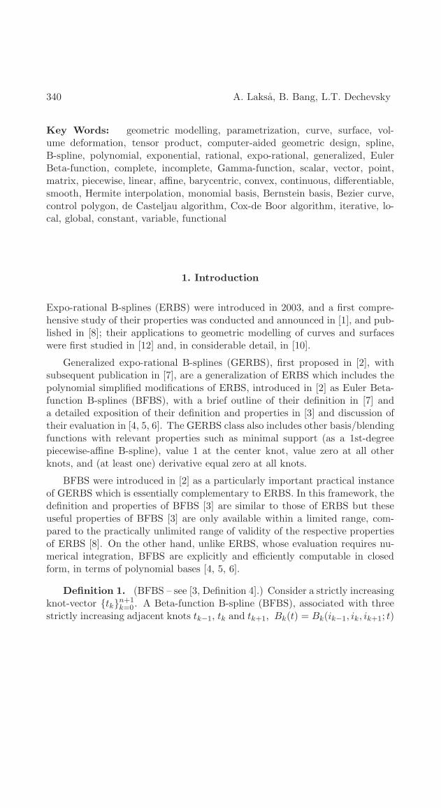
Theorem 1. Let the sequence of functions ck : [sk0, sk1] ⊂ R →R

d where 1 ≤ d <∞, be ∈ F(Bk). Let

f(t) =

n∑

k=1

ck ◦ ωk(t)Bk(t) (10)

be the general “BFBS” d-dimensional vector function, defined by the knotvector {tk}

n+1k=0 and the local vector functions ck(s), k = 1, ..., n. Denote the

global/local “scaling” factors by

δk =sk1 − sk0

tk+1 − tk−1, for k = 1, 2, ..., n. (11)

If the assumptions in [3, Theorem 1] are fulfilled, then

Djf(tk) = δjk D

jck ◦ ωk(tk), for j = 0, 1, 2, ..., ik and k = 1, .., n. (12)

Proof. Deriving (10) with respect to t, we get

Df(t) =n∑

k=1

(D(ck ◦ ωk)(t)Bk(t) + ck ◦ ωk(t)DBk(t)) .

Recalling that Bk(tk) = 1 (property Q1(a) in [3, Theorem 1]), Bk(tj) = 0 whenj 6= k (property Q2 in [3, Theorem 1]) and DjBk(tk) = 0 for all j = 1, . . . , ik(property Q1((d1).1) in [3, Theorem 1]), it follows that

Df(tk) = D(ck ◦ ωk)(t)

= δk Dck ◦ ωk(t).

Since

D(Djck ◦ ωk)(t) = δk Dj+1ck ◦ ωk(t),

expression (12) follows.

Remark 2. One typical situation is when the domain of the local functionis scaled to the standard “unit” domain. For example, Bezier curves have adomain where sk1 − sk0 = 1. Combined with a uniform knot vector wheretk+1 − tk−1 = 1 for k = 1, ..., n, the scaling factor δj

k for k = 1, ..., n andfor j = 1, 2, ... can be eliminated from consideration, which is very convenientpractically. In all other cases it is important to remember these importantscalings!


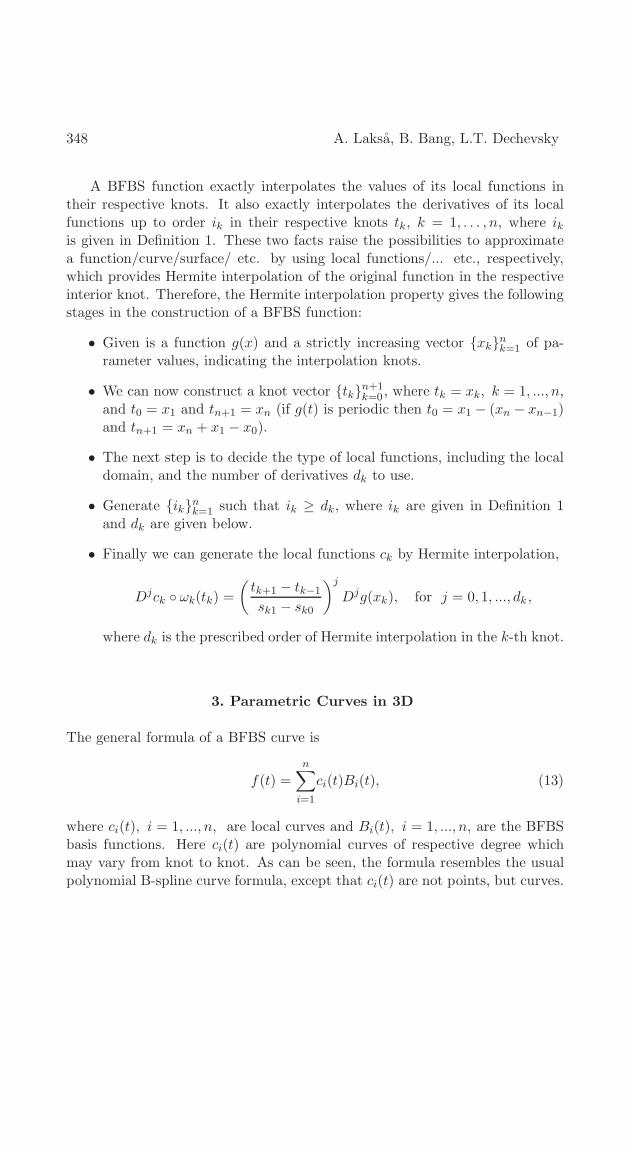
A BFBS function exactly interpolates the values of its local functions intheir respective knots. It also exactly interpolates the derivatives of its localfunctions up to order ik in their respective knots tk, k = 1, . . . , n, where ikis given in Definition 1. These two facts raise the possibilities to approximatea function/curve/surface/ etc. by using local functions/... etc., respectively,which provides Hermite interpolation of the original function in the respectiveinterior knot. Therefore, the Hermite interpolation property gives the followingstages in the construction of a BFBS function:

• Given is a function g(x) and a strictly increasing vector {xk}nk=1 of pa-

rameter values, indicating the interpolation knots.

• We can now construct a knot vector {tk}n+1k=0 , where tk = xk, k = 1, ..., n,

and t0 = x1 and tn+1 = xn (if g(t) is periodic then t0 = x1 − (xn − xn−1)and tn+1 = xn + x1 − x0).

• The next step is to decide the type of local functions, including the localdomain, and the number of derivatives dk to use.

• Generate {ik}nk=1 such that ik ≥ dk, where ik are given in Definition 1

and dk are given below.

• Finally we can generate the local functions ck by Hermite interpolation,

Djck ◦ ωk(tk) =

(tk+1 − tk−1

sk1 − sk0

)j

Djg(xk), for j = 0, 1, ..., dk ,

where dk is the prescribed order of Hermite interpolation in the k-th knot.

3. Parametric Curves in 3D

The general formula of a BFBS curve is

f(t) =n∑

i=1

ci(t)Bi(t), (13)

where ci(t), i = 1, ..., n, are local curves and Bi(t), i = 1, ..., n, are the BFBSbasis functions. Here ci(t) are polynomial curves of respective degree whichmay vary from knot to knot. As can be seen, the formula resembles the usualpolynomial B-spline curve formula, except that ci(t) are not points, but curves.


Figure 3: An approximate (global) BFBS curve (red) with four localcurves (green). The global curve is a blending of its local curves, withthe BFBS being the blending functions. The global curve also com-pletely interpolates all existing derivatives of each of the adjacent localcurves at the “middle” knot up to the respective multiplicity. In agreyscale version of the image, all colours used range within differentranges of the greyscale value.

The BFBS can, therefore, be viewed as a blending of local curves. Figure 3shows an example of a curve and its local blending curves.

Before we investigate different types of local curves, a comment is requiredon what it will look like using points as coefficients, as with ordinary B-splines.

Remark 3. (See also [8] for the case of ERBS, where this observation wasmade in the first place.) If we replace the local curves with points, the completecurve will geometrically be a piecewise linear curve with an infinitely smoothparametrization (on a strictly increasing knot vector) and DjBk(tl) = 0 (basicproperty Q4, see [3, Theorem 1]) implies that all derivatives of f must be zeroat every knot: Djf(tl) = 0, j = 1, 2, ..., s, s = min

k=1,...,nik, l = 1, ..., n, where il

is defined according to Definition 1 (this is illustrated on the right-hand side inFigure 4). It follows that all higher derivatives (vectors) must be parallel to thecurve (line) and, thus, to the first derivative. Thus, every derivative of f willgeometrically form a ’star’ concentrated at the origin (see the left-hand side ofFigure 4).

In Definition 2 the classification of local functions (functional coefficients)


Figure 4: (See also [8] for the case of ERBS.) The local curves arereplaced by points. The complete curve is on the right-hand side. Thestar, on the left-hand side, is the plot of the derivative centered at theorigin.

is given. For a vector-valued function (parametrized curve), the constraints onthe local function can be summed up in the following remark.

Remark 4. In principle, the only constraint on the choice of the localcurve ci(t) is that each of the coordinate components of ci(t) (which are scalar-valued functions) belongs to F(Bi) (Definition 2).

4. Definition/Implementation of “Open/Closed” Curves

For BFBS the definition and implementation of the ’open’ curves and ’closed’curves (see, e.g., [13] for the case of usual polynomial B-splines) is analogous aswith ERBS [10], with one difference: at the boundary of both the “open” andthe “closed” curves the respective number of Hermite interpolation conditionsis limited by i0 and in.

5. Evaluation of BFBS Curves and Their Derivatives

We can give a simple evaluation of the BFBS curve derivatives, using the Leibnizrule:

(f · g)(k) =k∑

j=0

(k

j

)f (j) · g(k−j),

we have

f (k)(t) =n∑

i=1

k∑

j=0

(k

j

)c(j)i (t)B

(k−j)i (t).


What happens in the interval between two adjacent knots? Some of the endsummands in the above sum at both ends are going to be zeroes, because theBFBS is polynomial. If we multiply the B-spline with a polynomial curve, wewill again obtain a piecewise polynomial. At one of the ends the derivative ofci(t) will be higher than its degree, so it is going to be zero. At the other endthe derivative of the B-spline is going to be too high, so again the result willbe zero. This is different from the case of ERBS where we obtain zeros onlyat one of the ends and only if the ci(t) is polynomial, because the ERBS basisfunction is not zero between two adjacent knots.

Let us give a matrix representation for the BFBS curve. We have

f(t) =

n∑

k=1

ck(t)Bk(t), (14)

where

ck(t) =

ik−1∑

µ=0

αµtµ, αµ = const. (15)

is a polynomial local curve.

We will rewrite equation (15) using Taylor’s formula,

ck(t) =

ik−1∑

µ=0

1

µ!c(µ)k (tk)(t− tk)

µ (16)

Now we can write ck(t) in matrix form using local monomial bases,

ck(t) = CMik,k(t), (17)

where

C =(c(µ)k (tk)

), µ = 0, . . . , ik−1,

is a row vector of dimension ik and has elements which are also vectors with allderivatives of ck(t) up to order ik − 1 at the knot tk.

Mik,k(t) is a column vector representation of the monomial basis centeredaround tk,

Mik,k(u) =

10!

(t−tk)1!...

(t−tk)ik−1

(ik−1)!

,


Mik ,k(t) is a column vector representation of the monomial basis centeredaround tk, where the monomial basis is normalized with 1

k! for the purposeof differentiation.

Let us change the monomial basis to Bernstein basis (cf. also [4, 5], wherethis change of basis was made indirectly):

Mik ,k(t) = AkBrik,k(t).

Now we can write (17) in the Bernstein basis

ck(t) = CAkBrik,k(t) (18)

where Ak is the matrix of the change between the two bases and it is withconstant coefficients. Brik,k is the Bernstein basis matrix.

The matrix representation of the BFBS curve, given in (14), is,

c(t) = (ck(t)) (Bn(t)) , (19)

where Bn is column vector with elements all BFBS basis function Bk(t), k =1, . . . , n.

Finally, we have the following matrix equation for the BFBS curve

c(t) = C Ak Brik,k(t) Bn(t). (20)

6. Bezier Curves as Local Curves

The theory of this type of local polynomial curves in the case of BFBS isthe same as for ERBS (see [8] and [10]), with the additional constraint that forBFBS the degree of the Bernstein basis for the local Bezier curve cannot exceedik in the interval [tk−1, tk+1]. For completeness, we give this standard theoryhere. Our exposition follows [10], Chapter 4: Curves, Section 3: Bezier curvesas local curves; an upgrade of this theory from Bernstein polynomial bases toclassical polynomial B-spline bases is derived in [11].

In general, Bezier curves are very convenient to use as local curves. Recallthat Bezier curves are defined by

c(t) =

d∑

i=0

ci bd,i(t), if 0 ≤ t ≤ 1, (21)

where the basis functions are the Bernstein polynomials


bd,i(t) =

(d

i

)ti (1 − t)d−i ,

and where ci ∈ Rn, i = 0, 1, ...d, are the coefficients and, thus, the control

polygon, d is the polynomial degree and where n is usually 2 or 3 (but can beany positive integer).

There are three different types of evaluators (computations of (21) used forBezier curves):

i) de Casteljau algorithm,ii) a Cox/de Boor type algorithm,iii) computing the Bernstein polynomials directly.

Hard-coded Bernstein polynomial gives the fastest algorithm for specific de-grees, but for general degrees a Cox/de Boor version of an algorithm is the mostflexible and also quite a fast algorithm. We will not, however, be focused on ageneral evaluator for Bezier curves, because this is well known and discussed inmany places. We shall, on the other hand, look in sufficient detail at a specificevaluator for use in both pre-evaluations and in the Hermite interpolation forgenerating local curves, when the local curves are Bezier curves.

The Generalized Bernstein/Hermite matrix will be introduced (interpola-tion matrices are discussed amongst others in [14]) for use in both Hermiteinterpolation and in pre-evaluation (both will be discussed later)

Bd(t, δ) =

bd,0 (t) bd,1 (t) . . . bd,d (t)

δ Dbd,0 (t) δ Dbd,1 (t) · · · δ Dbd,d (t)...

.... . .

...δdDdbd,0 (t) δdDdbd,1 (t) · · · δdDdbd,d (t)

. (22)

The special issue about this matrix (22) is the scaling δj , where j, the powerexponent, is the row number (the first row is numbered 0). The reason forthis scaling will be explained later. However, in general Hermite interpolation,δ = 1 holds. In the following, we shall introduce an algorithm to compute thisgeneralized version of the matrix. Later, we shall see how to use this matrix.

First, we have to look at another matrix; T(t) : Rk → R

k−1, defining thede Casteljau algorithm. This matrix is a band-limited matrix with bandwidthtwo, and with the elements 1 − t and t on the nonzero band.

We can now look at a matrix version of an n-th degree Bezier curve,

c(t) = T1(t)T2(t) . . . Tn(t)C, (23)


where the indices 1, 2, . . . n denote the number of rows in the respective matrixTi, i = 1, . . . , n. We will also write the general formula of a derivative of thiscurve.

c(k)(t) = n(n− 1) . . . (n− k + 1) T1(t)T2(t) . . . Tn−k(t) T′n−k+1T

′n−k+2 . . . T

′n C

=n!

(n − k)!

n−k∏

i=1, k<n

Ti(t)n∏

j=n−k+1

T ′j(t) C, k = 0, . . . , n.

(24)

The derivative of the matrix Ti(t), denoted T ′i , i = 1, . . . , n is a matrix inde-

pendent of t, a band-limited matrix with bandwidth two, and with the elements−1 and 1 on the band.

In the following equations we will see an example of (23) for 3rd degreeBezier curve and its three derivatives in matrix form,

c(t) = T1(t)T2(t)T3(t) C,c′(t) = 3 T1(t)T2(t) T

′3 C,

c′′(t) = 6 T1(t) T′2T

′3 C,

c′′′(t) = 6 T ′1T

′2T

′3 C,

If we expand these equations, we get the following matrix presentation for a3rd degree Bezier curve and its three derivatives,

c(t) =(

1 − t t) (

1 − t t 00 1 − t t

)

1 − t t 0 0

0 1 − t t 00 0 1 − t t

c1c2c3c4

,

c′(t) = 3(

1 − t t) (

1 − t t 00 1 − t t

)

−1 1 0 0

0 −1 1 00 0 −1 1

c1c2c3c4

,

c′′(t) = 6(

1 − t t) (

−1 1 00 −1 1

)

−1 1 0 0

0 −1 1 00 0 −1 1

c1c2c3c4

,

c′′′(t) = 6(−1 1

) (−1 1 0

0 −1 1

)

−1 1 0 0

0 −1 1 00 0 −1 1

c1c2c3c4

.


Now we can clearly see that:

i) If we compute from the right-hand side (skipping the zeros), we get the deCasteljau algorithm.

ii) If we compute from the left-hand side, we get an algorithm of Cox/de Boortype.

iii) If we multiply the matrices from the left-hand side, without the coefficientvector on the right-hand side, we will get the Bernstein polynomials andtheir derivatives.In Section 2.3, the Hermite interpolation properties are discussed. If the

domain of the Bezier curve is scaled, as is the norm, because of the global/localaffine mapping (see (8) in Definition 4), then, in order to compute, for instance,the local Bezier curve ci(t), the j-th derivatives actually have to be scaled bythe global/local “scaling factor” δj

i where

δi =1

ti+1 − ti−1, (25)

as described in Theorem 1. The numerator in the fraction is 1 because thedomain of Bezier curves is [0, 1]. Because the matrix (22) is supposed to be usedboth in Hermite interpolation and in the evaluation of local curves, this matrixhas to include the scaling, as described earlier. This leads to the algorithm inthe next subsection to generate the matrix Bd(t, δ) described in (22).

So far in this section, we considered as a detailed example the cubic Beziercurve. The same considerations are valid for the respective matrix representa-tion of every degree of the Bezier curve (this degree corresponding, respectively,to the dimension of the largest matrix in the matrix representation). The onlydifference between the BFBS-case and the ERBS-case is that in the former casethis degree/dimension cannot exceed ik, while as for the latter case there is nosuch limitation.

6.1. Local Bezier Curves and Hermite Interpolation

Hermite interpolation with BFBS is also analogous to the case of ERBS, withrespective constraints on the order of the Hermite interpolation in the knots.Our exposition follows [10], Chapter 4: Curves, Section 3.1: Local Bezier curvesand Hermite interpolation, with respective modifications related to the multi-plicity ik in the knot tk, k = 1, . . . ,m.

We start by recalling the settings from Section 2.3, and adapting them toBFBS curves.


• Given is a curve g(t), g : [tstart, tend] ⊂ R → Rn, where we might have

n = 1, 2, 3, ...,

• Given is a number of samples m > 1, and the number of derivatives{di}

mi=1 > 0 in each of the sampling points, to be used in the interpolation.

• Generate a knot vector by:– first set t1 = tstart,– then set tm = tend.– Then for i = 2, 3, ...,m− 1 generate ti so that ti−1 < ti, and wheretm−1 < tm.– Finally, t0 and tm+1 must be set according to the rules for “open/closed”curves.

• Generate a vector of integers {ik}mk=1, ik ≥ dk.

• Design a BFBS curve using the knot vector {ti}m+1i=0 , and generate local

curves, in such a way that the BFBS curve is interpolating {Djg(ti)}di

j=0,for i = 1, ...,m.

This looks like an adjustment of a general Hermite interpolation method usedfor generating an approximation of a curve. What is specific is the generationof the local curves.

First, recall that the domain of a Bezier curve is [0, 1]. Then, note fromTheorem 1 that (adjusted with the local domain for Bezier curves)

Djf(ti) = δji D

jci ◦ ωi(ti), for j = 0, 1, 2, ... and i = 1, ..,m,

where f(t) is the BFBS curve, ci(t) now are Bezier curves, and

ωi(ti) =ti − ti−1

ti+1 − ti−1

is the affine global/local mapping from Definition 4, and

δi =1

ti+1 − ti−1, for i = 1, 2, ...,m,

is the global/local scaling factor of the domain defined in Theorem 1. This showsthat the BFBS curve is, adjusted by the domain-scaling factor, interpolatingthe local curve ci(t) for all derivatives at the knot ti for i = 1, ...,m. We now get


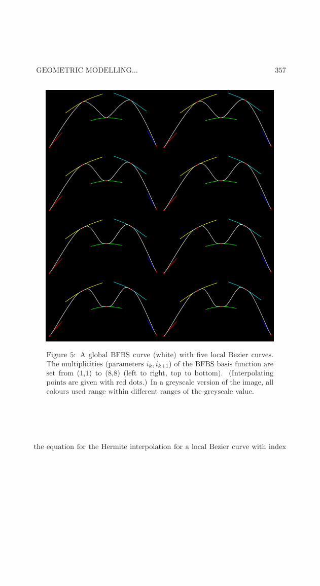
Figure 5: A global BFBS curve (white) with five local Bezier curves.The multiplicities (parameters ik, ik+1) of the BFBS basis function areset from (1,1) to (8,8) (left to right, top to bottom). (Interpolatingpoints are given with red dots.) In a greyscale version of the image, allcolours used range within different ranges of the greyscale value.

the equation for the Hermite interpolation for a local Bezier curve with index


i,

Dsg(ti) = Dsf(ti) = δsi D

sci◦ωi(ti) = δsi

di∑

j=0

ci,jDsbdi,j◦ωi(ti), for s = 0, ..., di.

This can be formulated in a vector/matrix form,

Bdi(ωi(ti), δi) ci = gi (26)

where Bdi(ωi(ti), δi) is the Bernstein/Hermite matrix described in equation

(22), and where

ci =

ci,0...ci,d

are the coefficients of the local Bezier curve with index i, and where

gi =

D0g(ti)

...Dd

i g(ti)

is a vector that is a typical result of an evaluator for a general parametrizedcurve.

The final step in the generation of the local Bezier curves is, thus, solvingequation (26) according to the Bezier coefficients ci,

ci = Bdi(ωi(ti), δi)

−1 gi. (27)

The conclusion is that, in order to compute the coefficient to the local Beziercurves (27), one has to compute the expanded Bernstein/Hermite matrix, then,invert this matrix, and multiply the inverted matrix with the “evaluation”-vector from the original curve. The matrix inversion will not be discussedfurther here, but there are many programming libraries available, includingoptimized algorithms for matrix inversions, see, e.g., [15].

For several reasons, it is advantageous to translate all coefficients after com-puting (27), so that the interpolation point is “in the local origin”. It follows,then, that we have to subtract g(ti) from all the coefficients in the control poly-gon ci of the local Bezier curve, and that we have to cancel this by insertingthe opposite movement to the graphical homogeneous matrix system. By ”ho-mogeneous matrix” we understand that the coordinates given in the matrix are


homogeneous. The premise is, of course, that this homogeneous matrix systemis involved in the total evaluator.

In Figure 5 one can see a global BFBS curve with five Bezier local curves.The multiplicities (parameters ik, ik+1) of the BFBS basis function are set from(1,1) to (8,8) (left to right, top to bottom). It is seen how the approximationat the knots (red dots) improves and approaches closer to the local curves andthe approximation in a neighbourhood of each knot becomes clearly visuallybetter with the raising of the multiplicity. The upper limit of order of Hermiteinterpolation in a point P (for approximation near the point) depends notonly on the smoothness of the curve, but also on ik, i.e., on the degree of thepolynomial density in the definition of BFBS at the point P .

Acknowledgments

This work was partially supported by the 2005, 2006, 2007, 2008 and 2009Annual Research Grants of the R&D Group for Mathematical Modelling, Nu-merical Simulation and Computer Visualization at Narvik University College,Norway.

The graphical images appearing in this exposition are selected from theimage gallery generated during the work of the students Ivana P. Ganchevaand Nedyalka D. Delistoyanova on their M.Sc. Diploma thesis [9] at NarvikUniversity College. In particular, we appreciate the good programming of IvanaP. Gancheva relevant to the M.Sc. Diploma thesis.

References

[1] L.T. Dechevsky, Expo-rational B-splines. Communication at the Fifth In-ternational Conference on Mathematical Methods for Curves and Surfaces,Tromsø 2004, Norway (unpublished).

[2] L.T. Dechevsky, Generalized expo-rational B-splines. Communication atthe Seventh International Conference on Mathematical Methods for Curvesand Surfaces, Tønsbeg 2008, Norway (unpublished).

[3] L.T. Dechevsky. Beta-function B-splines: definition and basic properties,Int. J. Pure Appl. Math., 65, No. 3 (2010), 279-295.

[4] L.T. Dechevsky. Evaluation of Beta-function B-splines, I: local monomialbases, Int. J. Pure Appl. Math., 65, No. 3 (2010), 297-310.


[5] L.T. Dechevsky. Evaluation of Beta-function B-splines, II: local Bernsteinbases, Int. J. Pure Appl. Math., 65, No. 3 (2010), 311-322.

[6] L.T. Dechevsky. Evaluation of Beta-function B-splines, III: global mono-mial bases, Int. J. Pure Appl. Math., 65, No. 3 (2010), 323-338.

[7] L.T. Dechevsky, A. Laksa, B. Bang. Generalized Expo-Rational B-splines,Int. J. Pure Appl. Math., 57(1) (2009) 833-872.

[8] L.T. Dechevsky, A. Laksa, B. Bang. Expo-Rational B-splines, Int. J. PureAppl. Math., 27(3) (2006) 319-369.

[9] I. P. Gancheva, N. D. Delistoyanova. Euler Beta-function B-splines: Defi-nition, Basic Properties, and Practical Use in Computer Aided GeometricDesign. M. Sc. Diploma thesis (supervisor: L. T. Dechevsky), Narvik Uni-versity College, Norway, 2007.

[10] A. Laksa. Basic Properties of Expo-Rational B-splines and Practical Usein Computer Aided Geometric Design, Doctor Philos. Dissertation, OsloUniversity, Unipub, Oslo, 606 (2007).

[11] A. Laksa. A Method for sparse-matrix computation of B-spline curves andsurfaces. In: Large-Scale Scientific Computing, 7th International Confer-ence, LSSC 2009, Lirkov, S. Margenov, J. Wasniewski (Eds.). LectureNotes in Computer Science 5910, 796-804, Springer, 2010.

[12] A. Laksa, B. Bang, L.T. Dechevsky. Exploring expo-rational B-splines forcurves and surfces. In: Mathematical methods for Curves and Surfaces,Tromsø’2004, M. Dæhlen and K. Mørken and L. Schumaker (eds.), 253-262, Nashboro Press, 2005.

[13] M. Mortenson. Mathematics for Computer Graphics Applications. Indus-trial Press, 1999.

[14] L.L. Schumaker. Spline Functions: Basic Theory. A Wiley-Intersciencepublication, John Wiley & Sons Inc., 1981.

[15] Wikipedia, The Free Encyclopedia: Basic Linear Algebra Subprograms.In: http://en.wikipedia.org/.

Documents

International Journal of Pure and Applied Mathematics · ume deformation, tensor product, computer-aided geometri c design, spline, B-spline ... (an a ne mapping) of the BFBS basis