Embed Size (px)
Citation preview
Research Report Agreement No.T9903, Task 95 Geosynthetic Reinforcement III
Washington State Department of Transportation Technical Monitor
Tony Allen Materials Laboratory Geotechnical Branch
Prepared for
Washington State Transportation Commission Department of Transportation
and in cooperation with U.S. Department of Transportation
Federal Highway Administration
January 2002
INTERNAL STABILITY ANALYSES OF GEOSYNTHETIC REINFORCED RETAINING WALLS
by
Robert D. Holtz Wei F. Lee Professor Research Assistant
Department of Civil and Environmental Engineering University of Washington, Bx 352700
Seattle, Washington 98195
Washington State Transportation Center (TRAC) University of Washington, Box 354802
University District Building 1107 NE 45th Street, Suite 535
Seattle, Washington 98105-4631

TECHNICAL REPORT STANDARD TITLE PAGE
1. REPORT NO. 2. GOVERNMENT ACCESSION NO. 3. RECIPIENT'S CATALOG NO.
WA-RD 532.1
4. TITLE AND SUBTITLE 5. REPORT DATE
INTERNAL STABILITY ANALYSES OF January 2002 GEOSYNTHETIC REINFORCED RETAINING WALLS 6. PERFORMING ORGANIZATION CODE 7. AUTHOR(S) 8. PERFORMING ORGANIZATION REPORT NO.
Robert D. Holtz, Wei F. Lee 9. PERFORMING ORGANIZATION NAME AND ADDRESS 10. WORK UNIT NO.
Washington State Transportation Center (TRAC) University of Washington, Box 354802 11. CONTRACT OR GRANT NO.
University District Building; 1107 NE 45th Street, Suite 535 Agreement T9903, Task 95 Seattle, Washington 98105-4631 12. SPONSORING AGENCY NAME AND ADDRESS 13. TYPE OF REPORT AND PERIOD COVERED
Research Office Washington State Department of Transportation Transportation Building, MS 47370
Final research report
Olympia, Washington 98504-7370 14. SPONSORING AGENCY CODE
Gary Ray, Project Manager, 360-709-7975 15. SUPPLEMENTARY NOTES
This study was conducted in cooperation with the U.S. Department of Transportation, Federal Highway Administration. 16. ABSTRACT
This research project was an effort to improve our understanding of the internal stress-strain distribution in GRS retaining structures. Our numerical modelling techniques utilized a commercially available element program, FLAC (Fast Lagrangian Analysis of Continua). In this research, we investigated and appropriately considered the plane strain soil properties, the effect of low confining pressure on the soil dilation angle, and in-soil and low strain rate geosynthetic reinforcement properties.
Modeling techniques that are able to predict both the internal and external performance of GRS walls simultaneously were developed. Instrumentation measurements such as wall deflection and reinforcement strain distributions of a number of selected case histories were successfully reproduced by our numerical modeling techniques. Moreover, these techniques were verified by successfully performing true “Class A” predictions of three large-scale experimental walls.
An extensive parametric study that included more than 250 numerical models was then performed to investigate the influence of design factors such as soil properties, reinforcement stiffness, and reinforcement spacing on GRS wall performance. Moreover, effects of design options such as toe restraint and structural facing systems were examined.
An alternative method for internal stress-strain analysis based on the stress-strain behavior of GRS as a composite material was also developed. Finally, the modeling results were used to develop a new technique for predicting GRS wall face deformations and to make recommendations for the internal stability design of GRS walls. 17. KEY WORDS 18. DISTRIBUTION STATEMENT
Geosynthetic, reinforcement, retaining wall, FLAC
No restrictions. This document is available to the public through the National Technical Information Service, Springfield, VA 22616
19. SECURITY CLASSIF. (of this report) 20. SECURITY CLASSIF. (of this page) 21. NO. OF PAGES 22. PRICE


iii
DISCLAIMER
The contents of this report reflect the views of the authors, who are responsible
for the facts and the accuracy of the data presented herein. The contents do not
necessarily reflect the official views or policies of the Washington State Transportation
Commission, Department of Transportation, or the Federal Highway Administration.
This report does not constitute a standard, specification, or regulation.

iv
v
TABLE OF CONTENTS
Section Page
EXECUTIVE SUMMARY ................................................................................. ix
1. INTRODUCTION ..................................................................................... 1
2. RESEARCH OBJECTIVES ....................................................................... 3
3. SCOPE OF WORK, TASKS, AND RESEARCH APPROACH ............... 4
3.1 Development of Numerical Techniques for Analyzing GRS Retaining Structure Performance ................................................................................ 4
3.2 Verification of the Developed Modeling Techniques................................. 4 3.2.1 Calibration of the Modeling Techniques by Using Case Histories ... 5 3.2.2 Update of the Modeling Techniques.................................................. 5 3.2.3 Prediction of the Performance of Large-Scale GRS Model Wall Tests 5
3.3 Performance of Parametric Study on the Internal Design Factors.............. 6 3.4 Development of Composite Method for Working Stress-Strain Analysis . 7 3.5 Improvement of GRS Retaining Wall Design ............................................ 8
4. MATERIAL PROPERTIES IN GRS RETAINING STRUCTURES ........ 9
5. DEVELOPING NUMERICAL MODELS OF GRS RETAINING STRUCTURES USING THE COMPUTER PROGRAM FLAC .............. 11
6. VERIFICATION OF NUMERICAL MODELING TECHNIQUES—REPRODUCING THE PERFORMANCE OF EXISTING GRS WALLS 13
7. PREDICTION OF THE PERFORMANCE OF FULL-SCALE GSR TEST WALLS....................................................................................................... 16
8. ANALYTICAL MODELS OF LATERAL REINFORCED EARTH PRESSURE AND COMPOSITE MODULUS OF GEOSYNTHETIC REINFORCED SOIL.................................................................................. 20
9. PARAMETRIC STUDY OF THE INTERNAL DESIGN FACTORS OF GRS WALLS ............................................................................................. 22
10. ANISOTROPIC MODEL FOR GEOSYNTHETIC REINFORCED SOIL COMPOSITE PROPERTIES ..................................................................... 25
11. APPLICATIONS OF MODELING RESULTS: PERFORMANCAE PREDICTION AND DESIGN RECOMMENDATIONS FOR GRS WALLS....................................................................................................... 27
11.1 Maximum Face Deflection ......................................................................... 28 11.2 Reinforcement Tension............................................................................... 29 11.3 Reinforcement Tension Distributions......................................................... 35 11.4 Limitations of the Performance Prediction Methods.................................. 37 11.5 Design Recommendations for GRS Walls.................................................. 37
12. CONCLUSIONS......................................................................................... 40

vi
12.1 Materials Properties in GRS Retaining Structures ..................................... 40 12.2 Performance Modeling of GRS Retaining Structures................................. 42 12.3 Parametric Study......................................................................................... 45 12.4 Anisotropic Model for Geosynthetic Reinforced Soil Composite
Properties .................................................................................................... 46 12.5 Performance Prediction and Design Recommendations of GRS
Retaining Structures.................................................................................... 47
13. REFERENCES ........................................................................................... 49 APPENDIX A. INTERNAL STABILITY ANALYSES OF GEOSYNTHETIC REINFORCED RETAINING WALLS............................................................... A-1

vii
LIST OF FIGURES
Figure Page
7.1 Normalized face deflections for GRS test walls with different foundations............................................................................. 19
7.2 Normalized maximum reinforcement tension distributions for GRS test walls with different foundations...................................... 19
11.1 Maximum face deflection versus GRS composite modulus .............. 28 11.2 Soil index of walls with different facing systems.............................. 32 11.3 Geosynthetic index of walls with different facing systems ............... 32 11.4 Design curves of soil index................................................................ 33 11.5 Design curve of geosynthetic index................................................... 34 11.6 Reinforcement tension distribution of GRS walls ............................. 36

viii
LIST OF TABLES
Table Page
11.1 Values of aT for different GRS walls ................................................. 35
ix
EXECUTIVE SUMMARY
Current internal stability analyses of geosynthetic reinforced soil (GRS) retaining
structures, such as the common tie-back wedge method and other methods based on
limiting equilibrium, are known to be very conservative. They have been found to over-
predict the stress levels in the reinforcement, especially in the lower half of the wall, and
because of that over-prediction, designs based on these methods are very uneconomical.
Furthermore, current design methods do not provide useful performance information such
as wall face deformations.
Previous research on this subject has had only limited success because (1) reliable
information on the internal stress or strain distributions in real GRS structures was
lacking; (2) numerical modeling techniques for analyzing the performance of GRS walls
have been somewhat problematic; and (3) GRS material and interface properties were not
well understood.
This research project was an effort to improve our understanding of the internal
stress-strain distribution in GRS retaining structures. Our numerical modelling techniques
utilized a commercially available element program, FLAC (Fast Lagrangian Analysis of
Continua). FLAC solves the matrix equations by means of an efficient and stable finite
difference approach. Large deformations are relatively easily handled, and in addition to
the traditional constitutive models, FLAC also permits the use of project-specific stress-
strain relations. In this research, we investigated and appropriately considered the plane
strain soil properties, the effect of low confining pressure on the soil dilation angle, and
in-soil and low strain rate geosynthetic reinforcement properties.

x
Modeling techniques that are able to predict both the internal and external
performance of GRS walls simultaneously were also developed. Instrumentation
measurements such as wall deflection and reinforcement strain distributions of a number
of selected case histories were successfully reproduced by our numerical modeling
techniques. Moreover, these techniques were verified by successfully performing true
“Class A” predictions of three large-scale experimental walls.
An extensive parametric study that included more than 250 numerical models was
then performed to investigate the influence of design factors such as soil properties,
reinforcement stiffness, and reinforcement spacing on GRS wall performance. Moreover,
effects of design options such as toe restraint and structural facing systems were
examined.
An alternative method for internal stress-strain analysis based on the stress-strain
behavior of GRS as a composite material was developed. Input properties for the
composite numerical models of GRS retaining structures were obtained from an
interpretation of tests performed in the unit cell device (UCD—Boyle, 1995), which was
developed in earlier research sponsored by the Washington State Department of
Transportation (WSDOT).
Finally, the modeling results were used to develop a new technique for predicting
GRS wall face deformations and to make recommendations for the internal stability
design of GRS walls.

xi
This research has contributed to progress in the following six specific topic areas
(chapters referred to below are in Lee, 2000, which is included as an appendix to this
report):
1. Better understanding of the material properties of GRS retaining structures: plane
strain soil properties and the effect of low confining pressure on the soil dilation angle
were carefully investigated in this research (Chapter 7).
2. Improved modeling techniques for working stress analyses of GRS retaining
structures: modeling techniques (Chapter 8) were developed to reproduce both the
external and internal working stress information from selected case histories (Chapter
9), as well as to perform “Class A” predictions on three well instrumented laboratory
test walls (Chapter 10). The results of this numerical modeling appeared to be
successful.
3. Improved analytical models for analyzing the behavior of GRS: in this research,
analytical models of the composite GRS modulus, lateral reinforced earth pressure
distribution (Chapter 11), and the stress-strain relationship of a GRS composite
element (Chapter 13) were developed to analyze the behavior of GRS and to validate
the results of numerical modeling.
4. The results of an extensive parametric study of GRS walls: an extensive parametric
study that included more than 250 numerical models was performed in this research.
Influences of design factors such as soil properties, reinforcement stiffness, and
reinforcement spacing on wall performance were carefully investigated. The effects
of design options such as toe restraint and structural facing systems on the
performance of the GRS walls were also examined (Chapter 12).

xii
5. Development of a composite approach for the working stress analysis of GRS
retaining structures: the developed analytical model of the GRS composite element
was used to examine the effects of the geosynthetic on reinforced soil performance, as
well as to develop composite numerical models for analyzing the performance of
GRS retaining structures (Chapter 13).
6. Development of performance prediction methods and design recommendations for
GRS retaining structures: performance prediction methods were developed on the
basis of the results of the modeling and the parametric study. Finally, this research
permitted reasonable but conservative recommendations for the internal stability
design of GRS retaining structures to be made (Chapter 14).

1
1. INTRODUCTION
Geosynthetics were introduced as an alternative (to steel) reinforcement material
for reinforced soil retaining structures in the early 1970s. Since then, the use of
geosynthetic reinforced soil (GRS) retaining structures has rapidly increased for the
following reasons:
1. Because of their flexibility, GRS retaining structures are more tolerant of
differential movements than conventional retaining structures or even concrete-
faced reinforced walls.
2. Geosynthetics are more resistant to corrosion and other chemical reactions than
other reinforcement materials such as steel.
3. GRS retaining structures are cost effective because the reinforcement is cheaper
than steel, and construction is more rapid in comparison to conventional retaining
walls.
Reinforced wall design is very similar to conventional retaining wall design, but
with the added consideration of internal stability of the reinforced section. External
stability is calculated in the conventional way; the bearing capacity must be adequate, the
reinforced section may not slide or overturn, and overall slope stability must be adequate.
Surcharges (live and dead loads; distributed and point loads) are considered in the
conventional manner. Settlement of the reinforced section also should be checked if the
foundation is compressible.
A number of different approaches to internal design of geotextile reinforced
retaining walls have been proposed, but the oldest and most common—and most

2
conservative—method is the tieback wedge analysis. It utilizes classical earth pressure
theory combined with tensile resisting “tiebacks” that extend behind the assumed
Rankine failure plane. The KA (or Ko) is assumed, depending on the stiffness of the
facing and the amount of yielding likely to occur during construction, and the earth
pressure at each vertical section of the wall is calculated. This earth pressure must be
resisted by the geosynthetic reinforcement at that section.
Thus, there are two possible limiting or failure conditions for reinforced walls:
rupture and pullout of the geosynthetic. The corresponding reinforcement properties are
the tensile strength of the geosynthetic and its pullout resistance. In the latter case, the
geosynthetic reinforcement must extend some distance behind the assumed failure wedge
so that it will not pull out of the backfill.
The tie-back wedge design procedure is based on an ultimate or limit state, and
therefore it has the following disadvantages:
1. It tends to seriously over-predict the lateral earth pressure distribution within the
reinforced section.
2. It is unable to accurately predict the magnitude and distribution of tensile stresses
in the reinforcement.
3. It is unable to predict external (face) deformations under working stresses.
To improve predictions of the performance of GRS retaining structures and to
increase our confidence in their use, especially for permanent or critical structures,
reliable information on their face deformations and internal stress-strain distributions is
necessary. Furthermore, overly conservative designs are also uneconomical, so
considerable cost savings can result from improved design procedures.

3
2. RESEARCH OBJECTIVES
The objectives of this project were as follows:
1. Develop numerical techniques capable of analyzing the performance of GRS
retaining structures. The numerical models should be able to provide useful
information on the internal stress-strain distribution and external wall
performance.
2. Verify the numerical modeling techniques by comparing the results of numerical
models of GRS retaining structures with the results of instrumentation and other
measurements from field and laboratory GRS wall tests.
3. Perform parametric studies on internal design factors such as layer spacing, the
strength properties of geosynthetic reinforcement, and facing stiffnesses, and
investigate their influence on the performance of GRS retaining structures.
4. Develop a method for internal stress-strain analysis based on the stress-strain
behavior of GRS as a composite material. Composite modulus properties of GRS
are obtained from the unit cell device (UCD—Boyle, 1995) and used as input
properties for the composite numerical models of GRS retaining structures.
5. Provide recommendations for predicting the performance of and improving the
internal design procedures for GRS retaining structures.

4
3. SCOPE OF WORK, TASKS, AND RESEARCH APPROACH
This section outlines our approach to accomplishing the above research
objectives.
3.1 Development of Numerical Techniques for Analyzing GRS Retaining Structure Performance
In this task, numerical models of GRS retaining structures were developed by
using the commercially available finite difference computer program FLAC (Fast
Lagrangian Analysis of Continua). A numerical model was first created for the Rainier
Avenue wall, a 12.6-m-high wrap-faced GRS wall designed and constructed by the
Washington State Department of Transportation (WSDOT) in Seattle, Washington. Once
the techniques of numerical modeling and FLAC programming were well understood,
this FLAC model was able to accurately reproduce field instrumentation measurements,
given properly determined input properties and realistic boundary conditions. Detailed
modeling techniques developed in this research are summarized in Section 5 below and
described in detail in Chapter 8 of Lee (2000)—See appendix.
3.2 Verification of the Developed Modeling Techniques
To verify the developed numerical modeling techniques, FLAC models of other
GRS retaining structures were also created using the same modeling techniques
developed for the Rainier Avenue wall. These models were developed to back-analyze
the performance results of instrumented case histories, as well as to predict the
performance of three large-scale instrumented model tests. Our approach was to (1)
calibrate the modeling techniques by using instrumented case histories, (2) update the
5
modeling techniques, and (3) predict the performance of three large-scale GRS model
wall tests.
3.2.1 Calibration of the Modeling Techniques by Using Case Histories
Performance data from five instrumented GRS retaining structures were obtained
and reproduced with the developed modeling techniques. The walls were from the
FHWA Reinforced Soil Project site at Algonquin, Illinois, and they included three
concrete panel walls, a modular block faced wall, and a wrap-faced wall. The purpose of
this task was to calibrate the developed modeling techniques so that they could be
universally applicable.
3.2.2 Update of the Modeling Techniques
Additional modeling techniques were developed in this task for structures with
different facings other than a wrapped face, with different boundary conditions, and with
different types of surcharging utilized in the Algonquin test walls. Modeling techniques
were updated during this task.
3.2.3 Prediction of the Performance of Large-Scale GRS Model Wall Tests
To further verify the developed modeling techniques, numerical models were
created of three large-scale GRS model walls built and tested at the Royal Military
College of Canada (RMCC). GRS walls tested in the laboratory provide advantages over
field tests in that they tend to have more uniform material properties, better
instrumentation measurements, incremental surcharge loadings, and simpler boundary
conditions. The RMCC tests were designed to systematically change the internal stability
design factors such as layer spacing and reinforcement stiffness. Appropriate adjustments
were made to the modeling techniques, material and interface properties, wall

6
construction sequence, and boundary conditions to improve the utility and accuracy of
the numerical models.
Although one wall was actually completed before modeling, true “Class A”
predictions, predictions made before the completion of wall construction, were performed
on two of the test walls to demonstrate the accuracy of the developed modeling
techniques.
3.3 Performance of Parametric Study on the Internal Design Factors
Another important task of this research was to examine the influence of the
internal design factors on the performance of GRS retaining structures. A parametric
study was performed on internal design factors such as layer spacing, ratio of
reinforcement length to wall height, soil properties, reinforcement properties, and facing
types.
Two types of parametric analyses were performed in this research. In the first
type, numerical models developed in previous tasks to model the performance of the
Rainier Avenue wall and the Algonquin FHWA concrete panel test walls were used as
the fundamental models of the parametric study. Major internal stability design factors
were systematically introduced into these two models. The analyses were performed by
varying only one design factor in each group at a time, while the other factors were fixed.
The second type of parametric study used a large number of GRS wall models
with different internal stability design factors. Design factors such as layer spacing, soil
strength properties, and reinforcement properties were systematically introduced into
these models to observe the effects of combinations of design factors.

7
Hypothetical GRS wall performance factors such as internal stress-strain levels
and face deformations were recorded and analyzed in both types of parametric analyses.
The purpose of the parametric study was to obtain a thorough understanding of the
influence of the major internal stability design factors on the performance of GRS
retaining structures. With a better understanding of the internal design factors, the
internal stability analysis and design of the GRS retaining structures can be improved.
3.4 Development of Composite Method for Working Stress-Strain Analysis
In this research, a composite method was developed to analyze the stress-strain
behavior of a GRS element, as well as the performance of GRS retaining structures. The
purpose of this part of the research was to evaluate the feasibility of using the composite
approach to provide working stress-strain information about GRS retaining structures.
Moreover, in a real design project, time and cost might limit the conduct of complicated
numerical analyses. Thus, the composite method for a working stress analysis could
quickly offer working stress-strain information for preliminary investigations and design,
provided that sufficient composite GRS properties were available.
An analytical model that treats the GRS composite as a transversely isotropic
homogenous material was developed and used to reduce GRS composite test data
obtained from unit cell device test results (Boyle, 1995) to obtain the composite
properties of GRS. Composite numerical models were then developed with composite
GRS properties as the input properties. Since the composite GRS properties are the only
inputs for the composite numerical models, less computation and iteration time were
necessary. Moreover, information on the anisotropy of the internal stress distributions of

8
GRS retaining structures was obtained from the results of the composite numerical
models.
3.5 Improvement of GRS Retaining Wall Design
The development of a practical and accurate design procedure for GRS retaining
structure systems was the most important objective of this research. Knowledge of the
influence of various design factors obtained from the previous tasks was used to develop
an improved design procedure and performance prediction method for GRS retaining
structures. Included was detailed information on modeling techniques, such as
determination of soil and geosynthetic properties, determination of the properties of the
interfaces between different materials, and FLAC programming.
9
4. MATERIAL PROPERTIES IN GRS RETAINING STRUCTURES
Successful working stress analyses rely very much on a good understanding of
input material properties. Material properties under working conditions must be carefully
investigated before working stress analyses are conducted. GRS retaining structures are
constructed of backfill soil, geosynthetic reinforcement, and facing units, if any.
Properties of these materials vary under different loading, deformation, or confinement
conditions. For example, properties such as the friction angle and the modulus of a soil
change when different loading conditions are applied. The stiffnesses of geosynthetics
are affected by the strain rate as well as by confinement.
In Chapter 7 of Lee (2000), the properties of the GRS wall construction materials
under loading conditions that occur inside these structures are discussed. Adjustments to
convert soil and geosynthetic properties obtained from conventional tests into conditions
inside the GRS walls are given, and the way to select these properties for numerical
models is described in detail. These adjustments can be summarized as follows:
1. Convert triaxial or direct shear soil friction angles to plane strain soil friction angles
using Equations 7.1.1 and 7.1.2 in Chapter 7.
2. Calculate the plane strain soil modulus using the modified hyperbolic soil modulus
model.
3. Determine the appropriate dilation angles of the backfill material.
4. Investigate the effect of soil confinement on reinforcement tensile modulus.
5. Apply the appropriate modulus reduction on reinforcement tensile modulus to
account for the low strain rate that occurs during wall construction.

10
Inaccurate input of material properties appears to be one of the major reasons that
working stress analyses have not been successfully performed on GRS walls. The
adjustments of material properties summarized above were utilized in this research to
model the performance of GRS walls, and successful modeling results were obtained.
Detailed descriptions of how these adjustments are implemented in the modeling
techniques for GRS retaining structure performance prediction are presented in the next
section and in Chapter 8 of Lee (2000).

11
5. DEVELOPING NUMERICAL MODELS OF GRS RETAINING STRUCTURES USING THE COMPUTER PROGRAM FLAC
In this research, numerical analyses were performed with the finite difference-
based computer program FLAC (Fast Lagrangian Analysis of Continua). FLAC was
selected because of its excellent capability to model geotechnical engineering related
problems and its flexible programming capability. Although numerical analyses using
the finite difference methods usually have much longer iteration times than finite element
methods (FEM), with the general availability of high-speed digital personal computers,
this is not a major shortcoming. Both discrete and composite models were developed
with the FLAC program.
Details of the development of numerical models with the FLAC program are
described in Chapter 8 of Lee (2000). After a general description of FLAC, the various
stress-strain models provided by FLAC are briefly described. These include the isotropic
elastic, transversely isotropic elastic, Mohr-Coulomb elasto-plastic, and a pressure
dependent soil modulus models. Next is a description of the interface elements and cable
elements used to model the reinforcement. The various techniques used to develop
numerical models for analyzing the performance of GRS structures are described in some
detail; these include a discussion of the model generation, boundary conditions,
equilibrium criteria, and the hyperbolic soil modulus model specifically developed for
this research. Next are discussions of how the reinforcement input properties are
determined and how the arrangement of the reinforcement, facing systems, arrangement
of interfaces, and wall construction are modeled. Finally, the chapter ends with a
discussion of modeling results and data reduction.

12
In conclusion, the modeling techniques used to predict the performance of GRS
retaining structures appear to be very complicated, especially when structural facing
systems are involved. The modeling techniques described in this chapter were obtained
from numerous trials and elaborate model calibrations. They provided the basic concepts
and the specific procedures needed to improve the working stress analyses of GRS
retaining structures with FLAC. A prerequisite for using these modeling techniques is a
good understanding of the in-structure material properties. Recall that the properties of
both soil and geosynthetic reinforcement have to be carefully determined, as described
earlier and in Chapter 7 of Lee (2000).

13
6. VERIFICATION OF NUMERICAL MODELING TECHNIQUES – REPRODUCING THE PERFORMANCE OF EXISTING GRS WALLS
Performance data from four instrumented GRS retaining structures and two steel
reinforced retaining structures were obtained and used to verify the numerical modeling
techniques described above. These case histories were chosen because they were fully
instrumented during construction, and the results of the instrumentation were well
documented. These case histories included the WSDOT geotextile wall at the west-
bound I-90 preload fill in Seattle, Washington, and five of the test walls constructed at
the FHWA Reinforced Soil Project site at Algonquin, Illinois.
Development of reasonable numerical models for these case histories, as well as
their proper calibration, required the development of numerous trial models and much
arduous work. The modeling results are presented and compared to the field
measurements from the six case histories in Chapter 9 of Lee (2000).
The results of the verification modeling of the six case histories led to the
following conclusions:
1. Numerical models developed with modeling techniques summarized above in Section
5 and in detail in Chapter 8 of Lee (2000) were able to reproduce both the external
and internal performance of GRS walls within reasonable ranges.
2. Accurate material properties are required to successfully model the performance of
GRS walls. The material property determination procedures summarized above in
Section 4 and in detail in Chapter 7 of Lee (2000) should be used.
3. For GRS walls with complicated facing systems such as modular blocks, accurate
face deflection predictions require correct input properties of the soil, the

14
geosynthetic, the interfaces between the blocks, and the reinforcement inserted
between the blocks. Interface properties can be determined with connection test data,
if available.
4. The modeling results indicated that the soil elements adjacent to the reinforcement
layers had smaller deformations than than soil elements located between the
reinforcements. This local bulging phenomenon occurred especially in the lower half
of the GRS walls or at the face of a wrap-faced wall where no structural facing units
confined the bulges.
5. Significant differences were found between the modeling results and inclinometer
measurements, especially above the locations of maximum wall deflections predicted
by the numerical models. The inclinometer measurements indicated a maximum wall
deflection at the top of the wall, while the modeling results indicated a maximum
deflection at about two-thirds of the height of the wall. Both predicted and measured
results of reinforcement strain distributions verified that the deflection predictions of
the numerical models and optical face survey were more reasonable than the
inclinometer measurements; i.e. only small deformation occurred at the top of the
GRS walls.
6. Even when insufficient material properties information was available and input
material properties had to be estimated from information on similar materials, the
numerical models developed in this research were able to provide reasonable working
strain information about the GRS walls
7. The results of one wrap-faced wall showed that the procedures used to determine the
in-soil stiffness from in-isolation test data for nonwoven geosynthetics were
15
appropriate. On the basis of the unit cell device tests on this material reported by
Boyle (1995), the input stiffness of the nonwoven geosynthetic reinforcement was
obtained by multiplying the 2 percent strain in-isolation stiffness by 5.0.
8. Reinforcement tensions calculated by the tie-back wedge method appeared to be
much higher, especially at the lower half of the wall, than those predicted by the
numerical models that were able to reproduce both the external and internal
performance of GRS walls. This observation confirms that the tie-back wedge design
method over-predicts the reinforcement tensions, especially in the lower part of the
wall. Possible reasons for this discrepancy are that the conventional lateral earth
pressure distributions are not modified for soil-reinforcement interaction and toe
restraint.
9. Modeling results showed that the actual locations of maximum reinforcement
tensions in GRS walls occurred at heights of between 0.2H to 0.5H, and not at the
bottom of the walls, as assumed by the tie-back wedge method.

16
7. PREDICTION OF THE PERFORMANCE OF FULL-SCALE GRS TEST
WALLS
As part of a program to build and test large-scale GRS walls in the laboratory of
the Royal Military College of Canada (RMCC), design factors such as reinforcement
stiffness and spacing were systematically changed. We were able to obtain the results of
instrumentation measurements of three of these walls from Dr. Richard Bathurst of
RMCC. We developed FLAC models of these test walls in an attempt to predict
performance before the walls were constructed (so-called “Class A” predictions). The
purposes of this exercise were to (1) further examine and improve the developed
modeling techniques, (2) investigate the effects of reinforcement stiffness and
reinforcement spacing on wall performance under high surcharges, and (3) examine the
feasibility of using the developed modeling techniques to perform parametric analyses of
design factors such as reinforcement stiffness and spacing.
Chapter 10 of Lee (2000) briefly describes the RMCC test program, as well as the
results of the Class A predictions. The differences between real walls and the
experimental walls tested in the laboratory are also discussed. The following is a
summary of the discussion and conclusions of this part of the research.
1. Numerical models tended to underpredict the wall face deflection at the end of the
construction by only about 6 to 10mm. The most likely reason for this
underestimation is that additional movement due to construction procedures such as
soil compaction was not considered in the FLAC models.

17
2. Numerical models tended to overestimate the wall face deflection at the top of the
wall after a surcharge had been applied. This result could be improved somewhat by
decreasing the contact area of the surcharge pressure. Full contact between the airbag
and backfill soil was assumed in the numerical models. During the tests of Walls 1
and 2, a decrease of the surcharge contact area (the area between the airbag and the
backfill soil) behind the wall face due to inflation of the airbag was observed,
however, the actual surcharge contact area was not reported, so the exact decrease in
surcharge contact area could not be modeled.
3. Overall, the FLAC models tended to underpredict the reinforcement strains in the
lower half of the test walls. A possible reason for this underestimation is that the
FLAC models did not model the toe restraint of the test wall very well.
4. By comparing the results of the modeling after the fact, predictions of wall
performance could be improved. For example, Test Wall 2 was constructed ith the
same geogrid as that used for Walls 1 and 3, but with every second longitudinal
member of the grid removed. This process was assumed to reduce the stiffness of the
geogrid by 50 percent; however, the actual stiffness reduction of this modified
geogrid was not measured, and no potential increase in stiffness of the geogrid due to
soil confinement was considered. Performance predictions have been improved
somewhat by increasing the reinforcement modulus to 70 percent of the original
modulus of this geogrid.
5. Both numerical models and post-construction observations of the test walls indicated
that large differential settlements occurred between the facing blocks and the backfill

18
soil. However, the strain gage measurements did not show any strain peaks near the
blocks.
6. The stiff concrete foundation of the test walls affected both the face deflection profile
and the reinforcement tension distribution, as shown in the normalized plots of
figures 7.1 and 7.2 from Lee (2000, Chapter 10). These figures show the results of
RMCC Wall 1 in comparison to the FHWA Algonquin modular block faced wall that
was described in Chapter 9 of Lee (2000). Figure 7.1 indicates that the maximum face
deflection of the wall with a stiff concrete foundation is located at top of the wall,
while that of the wall with a less stiff soil foundation is located near the middle of the
wall. Figure 7.2 also indicates that a stiff foundation has a similar effect on the
reinforcement tension distributions. The maximum reinforcement tension of the test
wall with a stiff concrete foundation occurred at a height of 0.8H, while the maximum
reinforcement tension of the test wall with a soil foundation occurred at a height of
0.5H.
Note that the performance predictions presented in this chapter are Class A
predictions, i.e., these modeling results were estimated before the construction of these
test walls. Refinement is always possible after prediction. For example, face deflection
predictions after surcharge could be further improved by decreasing the contact area of
the surcharge. Moreover, the performance simulation of test Wall 2 could be improved by
increasing the reinforcement modulus from 50 percent to 70 percent of the original
modulus of the geogrid used in test Walls 1 and 3.

19
Figure 7.1 Normalized face deflections for GRS test walls with different foundations.
Figure 7.2 Normalized maximum reinforcement tension distributions for GRS test walls with different foundations.
0
0.2
0.4
0.6
0.8
1
1.2
0 0.2 0.4 0.6 0.8 1 1.2
Normalized Wall Face Deflection (d/dmax)
Nor
mal
ized
Hei
ght (
h/H
) Algonquin modular blockfaced wall--soil foundation
RMCC test wall--stifffoundation
0
0.2
0.4
0.6
0.8
1
0 0.2 0.4 0.6 0.8 1 1.2
Normalized Maximum Reinforcement Tension (T/Tmax)
Nor
mal
ized
Hei
ght (
h/H
)
Algonquin modular blockfaced wall--soil foundationRMCC test wall--stifffoundation
20
8. ANALYTICAL MODELS OF LATERAL REINFORCED EARTH PRESSURE AND COMPOSITE MODULUS OF GEOSYNTHETIC REINFORCED SOIL
Two important design factors in current GRS wall design procedures are the
distribution of lateral earth pressure and the reinforcement stiffness. The lateral earth
pressure distribution is assumed, and the in-isolation stiffness of the geosynthetic
reinforcement is usually used. Available evidence from full-scale and model GRS walls
indicates that present design procedures tend to significantly overestimate the internal
lateral stress distribution within the structure, probably because of errors in both these
factors. The modeling results described in the section on verification also suggest that
the soil-only coefficients of lateral earth pressure and the in-isolation stiffness of
geosynthetics are not appropriate for characterizing the working stress or strain
distribution inside GRS walls.
To analyze the composite GRS behavior, two new terms, the coefficient of lateral
reinforced earth pressure, Kcomp, and composite modulus of geosynthetic reinforced soil,
Ecomp, were proposed by Lee (2000). The analytical models, derivations, and applications
of both Kcomp and Ecomp are described in Chapter 11 of Lee (2000).
Lee (2000) found that the GRS composite lateral earth pressure distribution is a
function of the height of the wall, unit weight and the lateral earth pressure coefficient of
the backfill soil, and the distribution of the reinforcement tension. He found that the
horizontal modulus of the GRS composite is a function of the stiffness of the
reinforcement, the vertical spacing of the reinforcement, and the soil modulus. Moduli
thus calculated are only appropriate for characterizing the horizontal working stress or
strain information of GRS walls. The in-soil and low strain rate adjustments discussed in

21
Chapter 7 of Lee (2000) have to be applied to the in-isolation reinforcement stiffness, and
the plane strain soil modulus should be used when GRS retaining structures are analyzed.
Es, the soil modulus, can be obtained from strength test data or estimated by using a
confining pressure dependent hyperbolic soil modulus model.

22
9. PARAMETRIC STUDY OF THE INTERNAL DESIGN FACTORS OF GRS WALLS
After the performance of the case histories and large-scale test walls had been
successfully predicted, extensive parametric studies were performed to investigate the
influence of internal design factors such as layer spacing, soil strength properties,
reinforcement stiffness, and facing types. The results of the parametric analyses were
recorded and analyzed in terms of GRS wall performance factors such as internal stress-
strain levels and wall face deflections. The purposes of the parametric study were to (1)
investigate the sensitivity of the modeling results to the input material properties, (2)
examine the influence of the internal design factors on the performance of GRS retaining
structures, and (3) improve the internal design of GRS walls on the basis of the working
stress information obtained from the parametric study.
Two types of parametric analyses were performed in this research. In the first
type, numerical models of the WSDOT Rainier Avenue wall and the FHWA Algonquin
concrete panel test walls were used as the fundamental models of the parametric study.
Internal design factors such as soil friction angle and reinforcement stiffness were
systematically varied in the models. These analyses were performed by varying only one
design factor at a time in each group while the other factors were fixed. The second type
of parametric study was performed by using a large number of GRS wall models with
different internal stability design factors. Design factors such as wall height, layer
spacing, soil strength properties, and reinforcement properties were systematically
introduced into GRS wall models to observe the effects of the interaction of these design

23
factors. The results of the parametric study are presented and discussed in detail Chapter
12 of Lee (2000); the summary and conclusions of this work follow.
1. Local failures were observed near the faces of GRS walls with larger vertical
reinforcement spacings. For wrap-faced GRS walls that were designed with the same
global stiffnesses but different vertical reinforcement spacings, the large spacing
walls exhibited much higher face deflections than the small spacing ones.
2. Face deformation of GRS walls was affected by both the strength properties of the
backfill and the global reinforcement stiffness. The parametric analysis results
indicated that the face deflections of GRS walls increased as the soil strength
decreased. Face deflections decreased as the global reinforcement stiffness increased.
A good correlation was found between the GRS composite modulus (Ecomp) and
normalized maximum face deflection (dmax/H).
3. Reinforcement tensions in GRS walls were affected by both the strength properties of
the backfill and the global reinforcement stiffness. The parametric analysis indicated
that overall reinforcement tensions in the GRS walls increased as the soil strength
properties decreased. Overall reinforcement tensions also increased as the global
reinforcement stiffness increased. However, the reinforcement tensions started to
increase when the walls were designed with very weak reinforcement because of the
large strains exhibited.
4. Toe restraint was able to reduce the maximum face deflections and reinforcement
tensions. Among three toe restraints investigated (0.05H embedment, 0.1H
embedment, and fixed toe), the 0.1H embedment was found to be the most effective

24
toe condition for improving the performance of GRS walls, especially for walls
designed with poor quality backfill.
5. For walls with large reinforcement spacings, secondary reinforcement was found to
be effective at improving the performance of walls only with good quality backfill.
Both the face deflections and reinforcement tensions of GRS walls with good quality
backfill could be decreased by using secondary reinforcement.
6. Structural facing systems such as modular blocks and concrete panels were able to
improve the stability and reduce the deformation of GRS walls, especially walls with
large spacings. Using structural facing systems could reduce maximum face
deflections, as well as the reinforcement tensions of wrap-faced walls with both large
and small spacing.
7. In contrast to the results of the tie-back wedge method, which predicts a maximum
reinforcement tension at the bottom of the wall, the parametric analyses indicated that
the maximum overall (average) reinforcement tensions occurred between 0.25H when
poor quality backfill was used to 0.5H when good quality backfill was used.

25
10. ANISOTROPIC MODEL FOR GEOSYNTHETIC REINFORCED SOIL COMPOSITE PROPERTIES
Instead of analyzing the geosynthetic reinforcement and soil separately, an effort
was made in this research to develop numerical analyses based on composite material
concepts. In the composite approach, the GRS element was considered to be a reinforced
composite material. A theory of anisotropic material under plane strain loading
conditions (described in Chapter 4 of Lee (2000) was used to analyze the different stress-
strain behavior in the different principal directions of the GRS composite.
The principal conclusions of this work are as follows:
1. Analyzing GRS composite properties with the developed transversely isotropic
elasticity model is feasible.
2. Different composite moduli of GRS elements were found in different principal
directions by using the transversely isotropic elasticity model. Thus, the assumption
that different reinforcing mechanisms exist in different principal directions inside a
GRS wall was verified.
3. Because the input GRS composite properties were sampled at an average working
strain found in the Rainier Avenue wall (1 percent), numerical models were able to
predict quite well the field instrumentation measurements. To improve this approach
so that it can be applied universally, the developed transversely isotropic elasticity
model for GRS elements should be applied to additional unit cell device test results.
The behavior of GRS composites sampled at different horizontal strains—for
example, 0.5 percent, 1.5 percent, and 2 percent—should be analyzed. The stress-

26
strain distribution of GRS retaining structures can then be further analyzed by using
composite property models with input of moduli sampled at these horizontal strains.
27
11. APPLICATIONS OF MODELING RESULTS: PERFORMANCE PREDICTION AND DESIGN RECOMMENDATIONS FOR GRS WALLS
In this section, methods for predicting GRS wall performance are presented.
These methods were developed in an effort to provide preliminary working stress design
information for GRS walls. The methods are based on the results of the parametric study
presented previously, and the general conditions for using these methods are as follows:
1. The walls have a vertical face. This is conservative.
2. The walls are built on a firm foundation; thus bearing capacity failure of the
foundation is not a concern.
3. The backfill extends behind the wall a distance equal to the embedded reinforcement
length from the end of the reinforcement. The foundation soil in front of the wall also
extends a distance equal to the embedded reinforcement length from the toe of the
wall. The depth of the foundation soil is at least equal to the height of the wall.
4. All layers of reinforcement inside each model wall have the same stiffness and
vertical spacing.
5. The ratio of reinforcement length to wall height is equal to 0.8.
The performance prediction methods summarized in the following sub-sections
include prediction of (1) maximum face deflections, (2) maximum reinforcement tension,
and (3) reinforcement tension distributions. The limitations of these prediction
procedures are described in detail. Design recommendations for GRS walls are
summarized at the end of this section. These recommendations are based on the results
of case history modeling and the parametric study presented earlier.

28
Example problems the illustrate the performance prediction methods are
presented in Lee (2000).
11.1 Maximum Face Deflection
A simplified method for predicting the maximum face deflection of GRS walls is
presented in Figure 11.1 (from Lee, 2000, Chapter 14). GRS walls were categorized into
three groups: (I) large spacing with a wrapped face, (II) large spacing with a structural
facing or small spacing with a wrapped face, and (III) small spacing with a structural
Figure 11.1 Maximum face deflection versus GRS composite modulus.
y = 2E+13x-3.1678
R2 = 0.898
y = 5E+11x-2.5827
R2 = 0.8261
y = 4E+13x-3.3262
R2 = 0.9484
0
10
20
30
40
50
60
70
80
0 5000 10000 15000 20000
Initial GRS Composite Modulus (kN/m^2)
Nor
mal
ized
Max
imum
Fac
e D
efle
ctio
n (m
m/m
)
Group I: large spacing with wrapped face
Group II: large spacing with structural facingsor small spacing with wrapped face
Group III: small spacing with structural facing
Group I
Group II
Group III

29
facing. The three curves in Figure 11.1 are the trend lines developed from the results of
the parametric study presented earlier. The GRS walls were designed with typical soils
(φ = 30 to 55 deg) and global reinforcement stiffnesses of between 500 to 5500 kN/m2.
The curves can be used to predict the face deflection if the material properties are known;
or they can be used to estimate required reinforcement stiffness if the soil properties and
tolerable deformation are known.
11.2 Reinforcement Tension
Maximum reinforcement tension can be estimated by using the analytical model
presented in Section 8 above and in Lee (2000, Chapter 11). (For ease of cross-
referencing, equation numbers in this report are the same as those in Lee, 2000).
Equation 11.1.6 is the expression for the accumulated reinforcement tension at a given
depth from the top of the wall. The reinforcement tension of an individual reinforcement
layer (Equation 14.2.2) is obtained by subtracting Equation 14.2.1 (the accumulated
reinforcement tension of layer n-1) from Equation 11.1.6.
)KK(2z
)z(t compsoil
2n
n
1i −⋅
⋅γ=∑ (11.1.6)
)KK(2z
)z(t compsoil
21n
1n
1i −⋅
⋅γ= −
−
∑ (14.2.1)
)zz()KK(2
ttt 21n
2ncompsoil
1n
1i
n
1in −
−
−⋅−⋅γ=−= ∑∑ (14.2.2)

30
Equation 14.2.2 can be rearranged as Equation 14.2.3, where zn - zn-1 = Sv, the
reinforcement spacing, and n1nn z
2)zz(
≈+ − . Reinforcement tension at a given layer can
then be expressed in terms of Sv and zn (Equation 14.2.4).
)zz()zz()KK(2
t 1nn1nncompsoiln −− +⋅−⋅−⋅γ= (14.2.3)
nvcompsoiln zS)KK(t ⋅⋅γ⋅−≈ (14.2.4)
The maximum reinforcement tension can be expressed by using Equation 14.2.5:
vmaxtcompsoilmax Sz)KK(T ⋅⋅γ⋅−=
vmaxtcompsoil SH
Hz)KK(
⋅⋅γ⋅⋅−
= (14.2.5)
where ztmax = depth of Tmax from top of the wall, and
H = height of wall.
As discussed in Section 8 and Chapter 11 of Lee (2000), the soil properties, as
well as the properties and arrangement of the reinforcement, control the values of Kcomp.
The results from the parametric study indicated that the locations of the maximum
reinforcement tensions were also affected by the soil properties. To analyze the modeling
results with Equation 14.2.5, two indices, a soil index and a geosynthetic index, were
defined to represent the term H
z)KK( maxtcompsoil ⋅−. Equation 14.2.5 can be rewritten as
Equation 14.2.6 by introducing these two indices into it.

31
vgsmax SHT ⋅⋅γ⋅Φ⋅Φ= (14.2.6)
where Φs = soil index, and
Φg = geosynthetic index.
Numerical and statistical analyses were performed on the average reinforcement
tension (Tave) results obtained from all the group models of the parametric study in
Chapter 12 of Lee (2000). The relationship between the soil index and soil properties, as
well as the relationship between the geosynthetic index and geosynthetic properties was
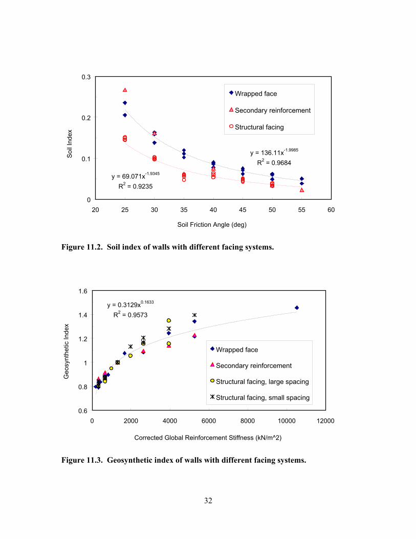
determined for GRS walls with different facing systems. Figure 11.2 (Lee, 2000, Chapter
14) shows the relation between the soil index and soil friction angles, and as shown in the
figure, very good correlation was found. Figure 11.3 (Lee, 2000, Chapter 14) shows the
relation between the geosynthetic index and the global reinforcement stiffnesses that
were corrected for in-soil confinement and low strain rate effects. As shown in the
figure, very good correlation was also found in this case for all models; however, the
geosynthetic indices were not affected very much by the facing systems (Figure 11.3).
32
Figure 11.2. Soil index of walls with different facing systems.
Figure 11.3. Geosynthetic index of walls with different facing systems.
y = 136.11x-1.9985
R2 = 0.9684
y = 69.071x-1.9345
R2 = 0.9235
0
0.1
0.2
0.3
20 25 30 35 40 45 50 55 60
Soil Friction Angle (deg)
Soil
Inde
x
Wrapped face
Secondary reinforcement
Structural facing
y = 0.3129x0.1633
R2 = 0.9573
0.6
0.8
1
1.2
1.4
1.6
0 2000 4000 6000 8000 10000 12000
Corrected Global Reinforcement Stiffness (kN/m^2)
Geo
synt
hetic
Inde
x
Wrapped face
Secondary reinforcement
Structural facing, large spacing
Structural facing, small spacing

33
Magnitudes of the maximum average reinforcement tensions (Tave_max) can be
estimated by using Equation 14.2.6. The soil and geosynthetic indices in this equation
can be determined by using figures 11.2 and 11.3. The design curves shown in figures
11.4 and 11.5 are the trend lines of the modeling results shown in figures 11.2 and 11.3.
Table 11.1 shows the average ratios (aT) of the maximum average reinforcement tension
to the maximum peak reinforcement tension (Tpeak_max / Tave_max) for all the models
analyzed in this study. The maximum peak reinforcement tensions (Tpeak) obtained from
the numerical models tended to over-predict the actual peak reinforcement tensions in the
GRS walls because the reinforcement elements were attached to the material element
nodes. (Details of this over-estimation are described in Section 8.5.6 of Lee, 2000.) In
comparison to the field measurements of the case histories analyzed in this research, Tpeak
obtained from the numerical models with reinforcement elements attached to the nodes
tended to over-predict the actual peak reinforcement tension by about 20 percent.
Figure 11.4. Design curves of soil index.
y = 136.11x-1.9985
R2 = 0.9684
y = 69.071x-1.9345
R2 = 0.9235
0
0.1
0.2
0.3
20 25 30 35 40 45 50 55 60
Soil Friction Angle (deg)
Soil
Inde
x
Wrapped face
Structural face

34
Figure 11.5. Design curve of geosynthetic index.
Maximum peak reinforcement tensions can be estimated by using aT and Equation
14.2.6 (Equation 14.2.7).
vgsTmax_aveTmax_peak SHaTaT ⋅⋅γ⋅Φ⋅Φ⋅=⋅= (14.2.7)
where aT = ratio of (Tpeak_max / Tave_max) (Table 14.2.1),
Φs = soil index, and
Φg = geosynthetic index.
y = 0.3035x0.1678
R2 = 0.9397
0.6
0.8
1
1.2
1.4
1.6
0 2000 4000 6000 8000 10000 12000
Corrected Global Reinforcement Stiffness (kN/m^2)
Geo
synt
hetic
Inde
x

35
Table 11.1 Values of aT for different GRS walls.
Wall Types aT
Wrap faced, large spacing (Sv = 0.76m) 1.8
Wrap faced, small spacing (Sv = 0.38m) 1.5
Wrap faced, with secondary reinforcement, large spacing 1.7
Modular block faced, large spacing 1.7
Modular block faced, small spacing 1.5
Concrete panel faced, large spacing 2.2
Concrete panel faced, small spacing 1.8
11.3 Reinforcement Tension Distributions
The results of the case histories, laboratory test walls, and parametric studies
indicated that the actual reinforcement tension distributions inside the GRS walls were
very different from the reinforcement tension distributions calculated, for example, with
the tie-back wedge method. The results of the parametric analysis indicated that the
locations of maximum reinforcement tensions occurred between 0.25H for poor quality
backfill to 0.5H for good quality backfill. The tie-back wedge method, of course,
predicts maximum reinforcement tension at the bottom of the wall. Moreover, the
modeling results presented in Section 6 and Chapter 9 of Lee (2000) also showed that the
actual reinforcement tensions inside GRS walls were smaller than the maximum
reinforcement tensions predicted by the tie-back wedge method.
Figure 11.6 shows a trapezoid reinforcement tension distribution for GRS walls. This
distribution was developed to cover all the reinforcement tension distributions that were
observed in the field measurements (Lee, 2000, Chapter 9) and the parametric study (Lee,
2000, Chapter 12). As shown in Figure 11.6, reinforcement tension increases from 0.2
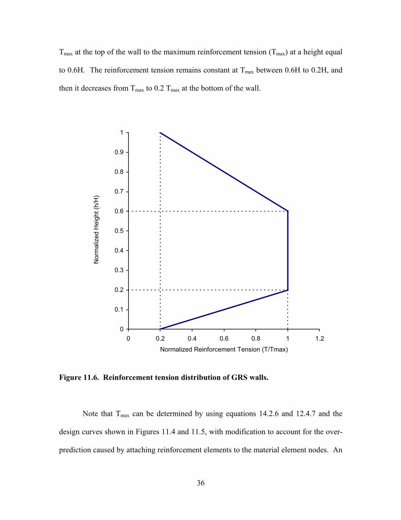
36
Tmax at the top of the wall to the maximum reinforcement tension (Tmax) at a height equal
to 0.6H. The reinforcement tension remains constant at Tmax between 0.6H to 0.2H, and
then it decreases from Tmax to 0.2 Tmax at the bottom of the wall.
Figure 11.6. Reinforcement tension distribution of GRS walls.
Note that Tmax can be determined by using equations 14.2.6 and 12.4.7 and the
design curves shown in Figures 11.4 and 11.5, with modification to account for the over-
prediction caused by attaching reinforcement elements to the material element nodes. An
0
0.1
0.2
0.3
0.4
0.5
0.6
0.7
0.8
0.9
1
0 0.2 0.4 0.6 0.8 1 1.2
Normalized Reinforcement Tension (T/Tmax)
Nor
mal
ized
Hei
ght (
h/H
)
37
example problem in Lee (2000) indicated that excellent prediction was obtained by using
the method presented in this chapter.
11.4 Limitations of the Performance Prediction Methods
The performance prediction methods presented in this chapter were developed on
the basis of the results of the extensive parametric study performed in this research
(Section 9 and Chapter 12 of Lee, 2000). The limitations of using these methods to
predict the performance of GRS walls include the wall geometry, boundary conditions,
soil properties, and reinforcement properties and arrangement that are similar to the
limitations for the numerical models of the parametric study. Details of these limitations
are described in Lee (2000).
11.5 Design Recommendations for GRS Walls
1. The results of the parametric study indicate that reinforcement lengths equal to 0.8H
(H is the height of the wall) seem to be adequate. Even models designed with very
poor quality backfill material (φ = 25 deg) or very weak reinforcement (J = 55 kN/m)
showed no failures in the backfill behind the reinforced zone. Only localized failures
were found at the face of wrapped walls with large spacing.
2. Reinforcement spacings larger than 0.6m are not recommended for use in wrap-faced
walls. Local failures were observed in the wrap-faced wall models with spacings
larger than 0.6m. The face deflection profiles and reinforcement tension distributions
of these large spacing wrap-faced wall models also indicated that these local failures
can cause internal instability such as outward rotation of the wall face.
3. Material properties such as plane strain soil properties and in-soil low strain rate
reinforcement stiffnesses have to be carefully investigated when GRS retaining

38
structures are designed. The modeling results in chapters 9 and 10 of Lee (2000)
indicated that the performance of GRS walls can be accurately reproduced with
correct material property information. To investigate the material properties inside
GRS retaining structures, the property determination procedures summarized in
Section 4 and detailed in Lee (2000, Chapter 7) can be used as a guideline.
4. If possible, good quality backfill (plane strain friction angle, φps, larger than 35 deg) is
recommended for the backfill material. The results of the parametric study indicated
that GRS walls designed with poor quality backfill would experience very large wall
face deflections as well as large reinforcement tensions.
5. Reinforcement stiffness was found to have less effect on the wall deflection and
reinforcement tensions of GRS walls than the soil quality. However, a global
stiffness (reinforcement stiffness divided by the spacing) of larger than 500 kN/m2 is
recommended for use in design.
6. Secondary reinforcement layers can only be used as an alternative facing system
when the backfill quality is good (φps > 35 deg). The wall deflections and
reinforcement tensions of wrap-faced walls with secondary reinforcement layers and
good quality backfill were very similarly to those of the small spacing wrap-faced
wall.
7. Structural facing systems are able to improve both the performance and internal
stability of the wrap-faced walls. As the parametric study indicated, both wall
deflection and reinforcement tensions were reduced when structural facing systems
were added in front of wrap-faced walls.

39
8. Preliminary design information such as maximum face deflection and reinforcement
tension distributions can be obtained by using the prediction methods described in
this section and Chapter 14 of Lee (2000).
9. With material properties and geometry known, the maximum face deflection of GRS
walls can be reasonably predicted by using Figure 11.1. Figure 11.1 can also be used
to determine the required reinforcement stiffness if soil properties and design
geometry are known.
10. Maximum reinforcement tension inside the GRS walls can be estimated by using
equations 14.2.6 and 14.2.7 and the design curves shown in figures 11.4 and 11.5.
11. Figure 11.6 shows a reinforcement tension distribution based on the working stress-
strain information from the parametric study.
12. For critical cases, a numerical analysis is still recommended so that complete working
stress-strain information can be obtained for internal stability. Determination of
material properties and modeling techniques as described in Chapters 7 and 8 of Lee
(2000) can be used as the “general rules” for performing the numerical analyses.
40
12. CONCLUSIONS
The main conclusions of this research are organized in terms of five
subcategories: 1. material properties in GRS retaining structures; 2. performance
modeling of GRS retaining structures; 3. parametric study; 4. anisotropic model for GRS
composite properties; and 5. performance prediction and design recommendations for
GRS retaining structures. The chapter references below refer to Lee (2000).
12.1 Material Properties in GRS Retaining Structures
1. The material properties inside the GRS retaining structures were found to be different
than those obtained by using conventional properties tests. To design GRS retaining
structures correctly, material properties such as plane strain strength properties of
soil, low confining pressure soil dilation angles, in-soil properties of geosynthetic
reinforcement, and low strain rate reinforcement stiffness need to be carefully
determined.
2. The plane strain soil friction angles of rounded uniform sand such as Ottawa sand
were found to be only slightly higher than triaxial friction angles. However, for
angular material, the tendency of soils to posses a higher friction angle under plane
strain conditions than under triaxial conditions is clear. The empirical equation
proposed by Lade and Lee (1976, Equation 7.1.1) was able to predict the plane strain
soil friction angle within a reasonable range.
3. The tendencies of plane strain soil moduli to be higher than triaxial soil moduli were
clearly supported by test data presented in Chapter 7 (Tables 7.1.2 to 7.1.4). For
uniform rounded material such as Ottawa sand, the plane strain 1 percent strain secant

41
moduli were only slightly higher than triaxial 1 percent strain secant moduli at low
confining pressures (20 to 100 kPa). For angular material, in both dense and loose
states, the plane strain 1 percent strain secant moduli were about twice as high as
those obtained from triaxial tests at low confining pressures (20 to 100 kPa).
4. Granular soils at low confining pressures possess higher dilation angles than those
tested under high confining pressures. For granular materials prepared in a dense
state, the low confining pressure dilation angles were as high as 40 deg. Even for
sands prepared in a loose state, the low confining pressure dilation angles were 26
deg. These dilation angles were determined on triaxial tests. Ideally, they should be
determined in plane strain tests.
5. The stiffness of nonwoven geosynthetics increased when the geosynthetics were
confined in soil. The increase of stiffness is controlled by the structure of the
geotextile and the confining pressure. At present, because of the difficulty of testing
geosynthetic reinforcement in soil, the magnitude of the increase in stiffness of the
nonwoven geosynthetic reinforcement is not well characterized and therefore needs
research.
6. For woven geotextiles, soil confinement seems to have less effect on stress-strain
behavior. The in-isolation stiffness of the woven geosynthetic can be used as the in-
soil reinforcement stiffness.
7. The strength properties of geosynthetic reinforcement were found to be affected by
the strain rate. Wide width tensile and unit cell device tests conducted at low strain
rates to simulate actual loading rates in full-scale structures have indicated that
reductions in reinforcement stiffness are needed. For nonwoven geotextiles, because
42
of the random fabric filaments and very different index properties between different
products, modulus reductions have not yet been clearly characterized. For woven
reinforcement and geogrids made of polypropylene, a 50 percent reduction of the in-
isolation modulus obtained from the wide width tensile test is recommended as the
low strain rate adjustment. For woven reinforcement and geogrids made of polyester,
a 20 percent reduction of modulus obtained from the wide width tensile test is
recommended. However, further research on this point is recommended.
8. Adjustments that convert soil and geosynthetic properties obtained from conventional
tests into those appropriate for GRS walls can be summarized as follows:
• Convert triaxial or direct shear soil friction angles to plane strain soil friction
angles using Equations 7.1.1 and 7.1.2.
• Calculate the plane strain soil modulus by using the modified hyperbolic soil
modulus model.
• Determine the appropriate dilation angles of the backfill material.
• Investigate the effect of soil confinement on reinforcement tensile modulus.
• Apply the appropriate modulus reduction to reinforcement tensile modulus to
account for the low strain rate that occurs during wall construction.
12.2 Performance Modeling of GRS Retaining Structures
1. Numerical models that were developed with the material property determination
procedures described in Chapter 7 and modeling techniques described in Chapter 8
were able to reproduce both the external and internal performance of GRS walls
within reasonable ranges.
2. Accurate and complete knowledge of material properties are the key to successfully

43
modeling the performance of GRS walls. Because information about the material
properties of the Rainier Avenue wall, Algonquin concrete panel faced wall, and
RMCC test walls was more complete, better predictions were made of those walls’
deflections and reinforcement strain distributions than for the other cases.
3. For GRS walls with complicated facing systems such as modular block facing,
accurate deflection predictions rely not only on the correct input properties of the soil
and geosynthetic, but also on the correct input properties of the interfaces between the
blocks and the reinforcement inserted between the blocks. The input properties of
reinforcement inserted between the blocks can be determined by using connection test
data, if available. More detailed modeling work is required to further refine the
working stress predictions of GRS walls with structural facings.
4. The modeling results indicated that soil elements adjacent to reinforcement layers
experienced smaller deformations than the elements in between the reinforcements.
This reinforcing phenomenon becomes more obvious especially at the lower half of
GRS walls or at the face of a wrap-faced wall,.
5. The inclinometer measurements indicated maximum wall deflection at the top of the
wall, while the modeling results indicated maximum deflection at about two-thirds of
the wall height. Both the predicted and measured results of reinforcement strain
distributions verified that the deflection predictions of the numerical models and
optical face survey were more reasonable than the inclinometer measurements, i.e.,
only small deformation occurred at top of the GRS walls.
6. The results of one wrap-faced wall showed that the procedures used to determine the
in-soil stiffness from in-isolation test data for nonwoven geosynthetics were

44
appropriate. On the basis of the unit cell device tests on this material reported by
Boyle (1995), the input stiffness of the nonwoven geosynthetic reinforcement was
obtained by multiplying the 2 percent strain in-isolation stiffness by 5.0.
7. Reinforcement tensions calculated by the tie-back wedge method appeared to be
much higher, especially at the lower half of the wall, than those predicted by the
numerical models that were able to reproduce both the external and internal
performance of GRS walls. This observation confirms that the tie-back wedge design
method over predicts reinforcement tensions, especially in the lower part of the wall.
A possible reason for this discrepancy is that the conventional lateral earth pressure
distributions are not modified for soil-reinforcement interaction and toe restraint.
8. The modeling results showed that the actual locations of maximum reinforcement
tensions in GRS walls occurred at heights of between 0.2H to 0.5H, and not at the
bottom of the walls, as assumed by the tie-back wedge method.
9. The numerical models of the RMCC laboratory test walls tended to underpredict the
wall face deflection at the end of the construction by only about 6 to 10mm. The most
likely reason for this underestimation is that additional movement due to construction
procedures such as soil compaction was not considered in the FLAC models.
10. The numerical models of the RMCC laboratory test walls also tended to overestimate
the wall face deflection at the top of the wall after a surcharge had been applied. This
result could be improved somewhat by decreasing the contact area of the surcharge
pressure.
11. Overall, the FLAC models of the RMCC test walls tended to underpredict the
reinforcement strains in the lower half of the test walls. A possible reason of this

45
underestimation is that the FLAC models did not model the toe restraint of the test
wall very well. Other discrepancies between the modeling results and actual
performance of the RMCC walls were described in Section 7 and Chapter 10 of Lee
(2000).
12.3 Parametric Study
1. Local failures were observed near the faces of the GRS walls with larger vertical
reinforcement spacings. For wrap-faced GRS walls that were designed with the same
global stiffnesses but different vertical reinforcement spacings, the large spacing
walls exhibited much higher face deflections than the small spacing ones.
2. Face deformation of the GRS walls was affected by both the strength properties of the
backfill and the global reinforcement stiffness. Parametric analysis results indicated
that the face deflections of the GRS walls increased as the soil strength decreased.
Face deflections decreased as the global reinforcement stiffness increased. A good
correlation was found between the GRS composite modulus (Ecomp) and normalized
maximum face deflection (dmax/H).
3. Reinforcement tensions in the GRS walls were affected by both the strength
properties of the backfill and the global reinforcement stiffness. Parametric analysis
indicated that overall reinforcement tensions in the GRS walls increased as the soil
strength properties decreased. Overall reinforcement tensions also increased as the
global reinforcement stiffness increased. However, the reinforcement tensions started
to increase when the walls were designed with very weak reinforcement because of
the large strains exhibited.
46
4. Toe restraints were able to reduce the maximum face deflections and reinforcement
tensions. Among three toe restraints investigated (0.05H embedment, 0.1H
embedment, and fixed toe), the 0.1H embedment was found to be the most effective
toe condition to improve the performance of GRS walls, especially for walls designed
with poor quality backfill.
5. For walls with large reinforcement spacings, secondary reinforcement was found to
be effective at improving the performance of only the walls with good quality
backfill. Both the face deflections and reinforcement tensions of GRS walls with
good quality backfill could be decreased by using secondary reinforcement.
6. Structural facing systems such as modular blocks and concrete panels were able to
improve the stability and reduce the deformation of GRS walls, especially walls with
large spacings. Use of structural facing systems could reduce maximum face
deflections, as well as the reinforcement tensions of wrap-faced walls with both large
and small spacing.
7. In contrast to the tie-back wedge method that predicts a maximum reinforcement
tension at the bottom of the wall, the results of the parametric analyses indicated that
the the maximum overall (average) reinforcement tensions occurred between 0.25H
where poor quality backfill was used to 0.5H when good quality backfill was used.
12.4 Anisotropic Model for Geosynthetic Reinforced Soil Composite Properties
1. Analysis of GRS composite properties with the developed transversely isotropic
elasticity model was demonstrated to be feasible.
2. Different composite moduli of GRS elements were found in different principal
directions by using the transversely isotropic elasticity model. Thus, the assumption
47
that different reinforcing mechanisms exist in different principal directions inside a
GRS wall was verified.
3. Because the input GRS composite properties were sampled at an average working
strain found in the Rainier Avenue wall (1 percent), numerical models were able to
predict quite well the field instrumentation measurements. To improve this approach
so that it can be more universally applicable, the developed transversely isotropic
elasticity model for GRS elements should be applied to additional unit cell device test
results. The behavior of GRS composites sampled at different horizontal strains—for
example, 0.5 percent, 1.5 percent, and 2 percent—should be analyzed. The stress-
strain distribution of GRS retaining structures can then be further analyzed by using
composite property models with input of moduli sampled at these horizontal strains.
12.5 Performance Prediction and Design Recommendations of GRS Retaining Structures 1. The performance prediction methods developed on the basis of the modeling and
analysis results are able to predict preliminary design information such as maximum
face deflection and reinforcement tension distributions.
2. With material properties and design geometry known, maximum face deflection of
GRS walls can be predicted by using Figure 11.1. The maximum face deflection that
was calculated in Figure 11.1 showed an excellent agreement with the field
measurements. Figure 11.1 can also be used to determine the required reinforcement
stiffness if soil properties and design geometry are known.
3. Procedures were developed to determine the maximum reinforcement tension inside
GRS walls.

48
4. Figure 11.6 describes a reinforcement tension distribution that was developed on the
basis of the working stress-strain information from the extensive parametric study
performed in this research.
5. Limitations to the performance prediction methods for GRS walls include the general
boundary conditions, ranges of the design factors, and geometry limits that are similar
to the limits of the numerical models of the parametric study.

49
13. REFERENCES
Boyle, S.R. (1995) “Deformation Prediction of Geosynthetic Reinforced Soil
Retaining Walls,” Ph.D. Dissertation, University of Washington, Seattle, 391p
Lade, P.V., and Lee, K.L. (1976) “Engineering Properties of Soils,” Report UCLA-ENG-
7652, 145pp.

50

Appendix A
Internal Stability Analyses of Geosynthetic Reinforced Retaining Walls
by
W e i F . L e e
A dissertation submitted in partial fulfillment of the requirements for the degree of
Doctor of Philosophy
University of Washington
Civil and Environmental Engineering
2000


University of Washington
Abstract
Internal Stability Analyses of
Geosynthetic Reinforced Retaining Walls
Wei Feng Lee
Chairperson of the Supervisory Committee:
Professor Robert D. Holtz Department of Civil and Environmental Engineering
Present internal stability analyses of geosynthetic reinforced soil (GRS) retaining structures are based on the limit state approach. Design methods based on this approach, such as tie-back wedge method, do not provide performance information of GRS walls and also have been found to over-predict the stress levels inside the GRS retaining structures. Working stress analyses of GRS walls are needed to improve the internal stability design as well as the performance prediction of the GRS walls. In this research, material properties such as plane strain soil properties, low confining pressure soil dilation angle, and in-soil and low strain rate geosynthetic reinforcement properties were carefully investigated. Modeling techniques that are able to predict both internal and external performance of GRS walls at the same time were also developed. Instrumentation measurements such as wall deflection and reinforcement strain distributions of the selected case histories were successfully reproduced by numerical models developed using these modeling techniques. Moreover, the developed modeling techniques were further verified by performing Class A predictions of three laboratory test walls. Results of the Class A predictions appear to be successful as well. An extensive parametric study that included more than 250 numerical models was then performed in this research. Influences of design factors of GRS walls such as soil properties, reinforcement stiffness, and reinforcement spacing on the performance were carefully investigated. Moreover, effects of design options such as toe restraint and structural facing systems on the performance of the GRS walls were also examined in this parametric study. In addition, analytical models of the composite GRS modulus and lateral reinforced earth pressure distribution that analyze the

behavior of the geosynthetic reinforced soil were also developed in order to analyze the results of the parametric study. In this research, effort was also made to develop the analytical model for the stress-strain relationship of a GRS composite element. The developed analytical model was used to examine the reinforcing effects of the geosynthetic reinforcement to the soil, as well as to develop composite numerical models for analyzing performance of GRS retaining structures. Finally new performance prediction methods based on the result of the parametric study and design recommendations for the internal stability design of GRS walls were obtained.
i
TABLE OF CONTENTS
List of Figures ix
List of Tables xx
Acknowledgments xxi
Chapter 1 Introduction 1
1.1 The Need to Improve the Internal Stability Design of GRS Retaining Structures
1
1.2 Research Overview 3
1.3 Thesis Organization 3
Chapter 2 Geosynthetic Reinforced Soil Retaining Structures 4
2.1 Retaining Structures 4
2.2 Reinforced Soil Retaining Structures: Externally Stabilized vs. Internally Stabilized Systems
5
2.3 Mechanism of Reinforced Soil Retaining Structures 8
2.4 Geosynthetic Reinforced Soil (GRS) Retaining Structures 12
2.4.1 Reinforcing Mechanisms 14
2.4.2 Interaction with Surrounding Soil 14
2.4.3 In-Soil and Low Strain Rate Reinforcement Stiffness 16
2.5 Stability of GRS Retaining Structures 17
2.5.1 External Stability 17
2.5.2 Internal Stability 17
Chapter 3 Internal Stability Analyses of GRS Retaining Structures 20
3.1 Concepts of Internal Stability Analyses of GRS Retaining Structures
21
3.1.1 Limit State Stress Analysis 23
3.1.2 Working Stress Analysis 24
3.2 Internal Stability Analyses of GRS Retaining Structures I--Limit State Design Methods
25
3.2.1 Lateral Earth Pressure Distributions 26
3.2.2 Reinforcement Tensile Forces 28
3.2.3 Reinforcement Pullout Forces 30

ii
3.3 Analytical Models of Reinforced Soil 31
3.3.1 Discrete Element Model 32
3.3.2 Composite Element Model 34
3.4 Internal Stability Analyses of GRS Retaining Structures II—Working Stress Design Methods and Numerical Analyses
36
3.4.1 Present Working Stress Design Method 36
3.4.2 Summary of Numerical Analysis Methods 37
3.5 Conclusions 42
3.5.1 Problems of Present Numerical Analyses Applications 42
3.5.2 Research Needs for Internal Stability Analyses of GRS Retaining Structures
43
Chapter 4 Elasticity Theory and Stress-Strain Interpretation Used to Develop the GRS Composite Model
45
4.1 Elasticity 45
4.1.1 Transversely Isotropic Elasticity 45
4.1.2 Plane Strain Loading Conditions 48
4.2 Stress-Strain Interpretations of a GRS Composite Element 50
Chapter 5 Research Objectives 53
Chapter 6 Scope of Work 55
6.1 Development of Numerical Techniques for Analyzing GRS Retaining Structure Performance
55
6.2 Verification of the Numerical Modeling Techniques 56
6.2.1 Calibration of the Modeling Techniques Using Case Histories
56
6.2.2 Update of the Modeling Techniques 56
6.2.3 Predict Performance of Large Scale GRS Model Wall Tests 57
6.3 Parametric Study on the Internal Design Factors 58
6.4 Composite Model for Working Stress-Strain Analysis 59
6.5 Improvement of GRS Retaining Wall Design 60
Chapter 7 Material Properties in GRS Retaining Structures 62
7.1 Soil Properties 62
7.1.1 Plane Strain Loading Conditions 65

iii
7.1.2 Plane Strain Soil Test Result 65
7.1.3 Summary of Plane Strain Soil Properties 79
7.1.4 Effects of Confining Pressure—Corrected Hyperbolic Soil Modulus Models for Plane Strain Conditions
82
7.1.5 Dilation Angle at Low Confining Pressure 85
7.2 Geosynthetic Properties 88
7.2.1 Material Types And Structures 88
7.2.2 Effect of Soil Confininement 91
7.2.3 Effect of Strain Rate 93
7.3 Conclusions 95
Chapter 8 Developing Numerical Models of GRS Retaining Structures Using Computer Program FLAC
96
8.1 General Description of FLAC 96
8.2 Built-in Material Models 99
8.2.1 Elastic Material Model 99
8.2.2 Transversely Isotropic Elastic Material Model 99
8.2.3 Mohr-Coulomb Material Model 100
8.2.4 Pressure Dependent Soil Modulus Model 101
8.3 Interface Elements 102
8.4 Cable Element—Structural Elements for Modeling Reinforcements
102
8.5 Techniques Used to Developing Numerical Models for Analyzing the performance of GRS Retaining Structures
104
8.5.1 Model Generation 105
8.5.2 Boundary Conditions 107
8.5.3 Equilibrium Criteria 108
8.5.4 Hyperbolic Soil Modulus Model 109
8.5.5 Determination of Reinforcement Input Properties 110
8.5.6 Arrangement of Reinforcement 112
8.5.7 Facing System 118
8.5.8 Input Property Determination and Arrangement of Interfaces 121

iv
8.5.9 Wall Construction 125
8.5.10 Mmodeling Result and Data Reduction 128
8.6 Conclusions 129
Chapter 9 Verification of Numerical Modeling Techniques—Reproducing Performance of Existing GRS walls
130
9.1 Introduction 130
9.2 Summary of the Case History and Their Numerical Models 132
9.2.1 WSDOT Rainier Avenue Geotextile Wall 132
9.2.2 Algonquin Precast Concrete Panel Faced Walls 134
9.2.3 Algonquin Modular Block Faced Wall 139
9.2.4 Algonquin Wrapped Face Wall 143
9.3 Modeling Result I—Wall Deflections 150
9.3.1 WSDOT Rainier Avenue Geotextile Wall 150
9.3.2 Algonquin Precast Concrete Panel Faced Walls 153
9.3.3 Algonquin Modular Block Faced Wall 156
9.3.4 Algonquin Wrapped Face Wall 159
9.3.5 Discussion and Conclusions 159
9.4 Modeling Result II—Reinforcement Strain Distribution 163
9.4.1 WSDOT Rainier Avenue Geotextile Wall 163
9.4.2 Algonquin Precast Concrete Panel Faced Walls 167
9.4.3 Algonquin Modular Block Faced Wall 171
9.4.4 Algonquin Wrapped Face Wall 171
9.4.5 Discussion and Conclusions 176
9.5 Modeling Result III—Reinforcement Tension Distributions 178
9.5.1 WSDOT Rainier Avenue Geotextile Wall 178
9.5.2 Algonquin Precast Concrete Panel Faced Walls 179
9.5.3 Algonquin Modular Block Faced Wall 182
9.5.4 Algonquin Wrapped Face Wall 182
9.5.5 Discussion and Conclusions 186
9.6 Summary and Conclusions 187

v
Chapter 10 Prediction of Performance of Full Scale GRS Test Walls. 190
10.1 Full Scale GRS Test Walls 191
10.2 Modeling Result 194
10.2.1 Wall 1 195
10.2.2 Wall 2 206
10.2.3 Wall 3 217
10.3 Difference Between Test Walls and Real Walls 223
10.4 Discussion and Conclusions 224
Chapter 11 Analytical Models of Lateral Reinforced Earth Pressure and Composite Modulus of Geosynthetic Reinforced Soil
229
11.1 Lateral Reinforced Earth Pressure 230
11.1.1 Analytical Models of Lateral Reinforced Earth Pressure 230
11.1.2 Values of Kcomp 236
11.1.3 Discussions and Conclusions 237
11.2 GRS Composite Modulus, Ecomp 240
11.2.1 Derivation of Ecomp 242
11.2.2 Conclusions And Discussions 244
Chapter 12 Parametric Study of the Internal Design Factors of GRS Walls
246
12.1 Introduction 247
12.2 Preliminary Parametric Study I -- Rainier Avenue Wall 250
12.3 Preliminary Parametric Study II – Algonquin Concrete Panel Walls
256
12.4 Analyses Matrix of the Major Parametric Study 258
12.4.1 General Boundary Conditions and Design Factors 259
12.4.2 Controlled Factor I—Backfill Soil Properties 259
12.4.3 Controlled Factor II—Reinforcement Stiffness and Spacing
259
12.4.4 Controlled Factor IV—Toe Restraint 261
12.4.5 Controlled Factor V—Facing Systems 261
12.5 Analysis Result I—Face Deflection 262

vi
12.6 Analysis Result II—Reinforcement Tension 269
12.6.1 Characterization of Reinforcement Tensions 269
12.6.2 Analysis Results 271
12.7 Analysis Result III—Effects of Toe Restraint 278
12.8 Analysis Result IV—Effects of Different Facing Systems 284
12.9 Summary and Conclusions 292
Chapter 13 Anisotropic Model for Geosynthetic Reinforced Soil Composite Properties
295
13.1 Behavior of Geosynthetic Reinforced Soil Element 295
13.2 Interpreting UCD Test Results Using the Tranversely Isotropic Elasticity Model
298
13.3 Composite GRS Moduli 300
13.4 Numerical Models Using Composite GRS Properties 308
13.5 Conclusions 313
Chapter 14 Application of Modeling Results: Performance Prediction and Design Recommendations for GRS Walls
313
14.1 Maximum Face Deflection 314
14.2 Reinforcement Tension 314
14.3 Reinforcement Tension Distributions 326
14.4 Limitations of the Performance Prediction Methods 328
14.4.1 Wall Geometry 328
14.4.2 Boundary Conditions 329
14.4.3 Soil Properties 330
14.4.4 Reinforcement Properties and Arrangement 330
14.5 Design Recommendations for GRS Walls 333
Chapter 15 Summary, Conclusions, and Recommendations for Future Researches
337

vii
15.1 Summary 337
15.2 Conclusions 340
15.2.1 Material Properties in GRS Retaining Structures 340
15.2.2 Performance Modeling of GRS Retaining Structures 342
15.2.3 Parametric Study 347
15.2.4 Anisotropic Model for Geosynthetic Reinforced Soil Composite Properties
349
15.2.5 Performance Prediction and Design Recommendations of GRS Retaining Structures
350
15.3 Future Researches 352
15.3.1 Material Properties in GRS Retaining Structures 352
15.3.2 Performance Modeling of GRS Retaining Structures 353
15.3.3 Parametric Study and Performance Prediction 354
15.3.4 Anisotropic Model for Geosynthetic Reinforced Soil Composite Properties
356
References 357
Appendix—Codes and Result Files of FLAC Models 379
viii
List of Figures
Figure 2.2.1 Examples of retaining wall systems. 7
Figure 2.3.1 Reinforcing mechanism of reinforced soil retaining structures. 10
Figure 2.3.2 Principal stress conditions of reinforced soil. 10
Figure 2.4.1 Examples of steel reinforcement: (a) steel straps, and (b) steel mats.
15
Figure 2.4.2 Examples of geosynthetic reinforcement: (a) geogrid, and (b) woven geotextile.
15
Figure 2.5.1 Failure models of segmental GRS retaining structures. 18
Figure 3.2.1 Various lateral earth pressure distributions. 27
Figure 3.3.1 Material properties involved in the development of the analytical models.
33
Figure 4.1.1 A schematic sketch of Equation 4.1.1. 46
Figure 4.1.2 A material element under plane strain loading condition. 49
Figure 4.2.1 Stress condition of a reinforced soil composite. 49
Figure 7.1.1 A material element under plane strain loading conditions. 66
Figure 7.1.2 A material element under typical triaxial loading conditions. 66
Figure 7.1.3 Grain size distributions of three tested soils. 67
Figure 7.1.4 Plane strain test results for Ottawa sand. 69
Figure 7.1.5 Triaxial test results for Ottawa sand. 70
Figure 7.1.6 Plane strain test results for Rainier sand. 72
Figure 7.1.7 Triaxial test results for Rainier sand. 73
Figure 7.1.8 Plane strain test results for RMC sand. 76
Figure 7.1.9 Triaxial test results for RMC sand. 77
Figure 7.1.10 Hyperbolic curve fitting for triaxial test data of RMC sand (K = 850, Rf = 0.73, n = 0.5).
84

ix
Figure 7.1.11 Hyperbolic curve fitting for plane strain test data of RMC sand(K = 2000, Rf = 0.73, n = 0.5).
84
Figure 8.1.1 Typical section of a GRS retaining structure modeled using FLAC.
98
Figure 8.3.1 Mechanical representation of the interface. 104
Figure 8.4.1 Material behavior of the cable element. 104
Figure 8.5.1 Effects of attaching cable elements to the material element nodes.
116
Figure 8.5.2 Typical section of concrete panel GRS walls modeled using FLAC.
120
Figure 8.5.3 Typical section of modular block GRS walls modeled using FLAC.
120
Figure 8.5.4 Construction procedures of a GRS wall modeled in FLAC. 127
Figure 9.2.1 Typical cross section of Rainier Avenue Geotextile wall. 133
Figure 9.2.2 Instrumented wall section of Rainier Avenue wall. 135
Figure 9.2.3 Wall geometry and instrumentation plan for Wall 2. 138
Figure 9.2.4 Cross section and material properties of Algonquin modular block faced test wall.
141
Figure 9.2.5 Instrumentation section of the Algonquin modular block faced geogrid wall.
142
Figure 9.2.6 Typical cross section and material properties of Algonquin wrapped faced wall.
146
Figure 9.2.7 Instrumentation section of the Algonquin wrapped faced wall. 147
Figure 9.3.1 Face deflection of Rainier Avenue wall: (a) end of construction, and (b) after surcharge.
151
Figure 9.3.2 Wall deformation of Rainier Avenue wall at 2.75m behind the wall face: (a) end of construction, and (b) after surcharge.
152
Figure 9.3.3 Predicted and measured wall face deflection of Algonquin concrete panel faced Wall 2 (geogrid wall).
154
Figure 9.3.4 Predicted and measured wall face deflection of Algonquin concrete panel faced Wall 1 (steel strips wall).
154
Figure 9.3.5 Predicted and measured wall face deflection of Algonquin concrete panel faced Wall 3 (steel bar mats wall).
155
Figure 9.3.6 Predicted and measured wall face deflection of Algonquin modular block faced wall
157
x
modular block faced wall.
Figure 9.3.7 Predicted and measured wall face deflection (2.7 m behind the wall face) of Algonquin modular block faced wall.
158
Figure 9.3.8 Predicted face deflection of Algonquin wrapped faced wall. 160
Figure 9.4.1 Predicted and measured reinforcement strain distributions of Rainier Avenue wall, end of construction.
164
Figure 9.4.2 Predicted and measured reinforcement strain distributions of Rainier Avenue wall, after surcharge.
165
Figure 9.4.3 Predicted and measured reinforcement strain distributions of Algonquin concrete panel faced Wall 2 (geogrid reinforced).
168
Figure 9.4.4 Predicted and measured reinforcement strain distributions of Algonquin concrete panel faced Wall 1 (steel reinforced).
169
Figure 9.4.5 Predicted and measured reinforcement strain distributions of Algonquin concrete panel faced Wall 3 (steel reinforced).
170
Figure 9.4.6 Predicted and measured reinforcement strain distribution of Algonquin modular block faced wall, end of construction.
172
Figure 9.4.7 Predicted and measured reinforcement strain distributions of Algonquin modular block faced wall, after surcharge.
173
Figure 9.4.8 Predicted and measured reinforcement strain distributions of Algonquin wrapped face wall, end of construction.
174
Figure 9.4.9 Predicted and measured reinforcement strain distributions of Algonquin wrapped face wall, after removing the retaining water.
175
Figure 9.5.1 Distribution of reinforcement tensions of Rainier Avenue wall. 180
Figure 9.5.2 Distribution of reinforcement tensions of Algonquin concrete panel faced geogrid wall.
181
Figure 9.5.3 Distributions of reinforcement tensions of Algonquin concrete panel faced walls.
183
Figure 9.5.4 Distributions of reinforcement tensions of Algonquin modular block faced wall.
184
Figure 9.5.5 Distribution of reinforcement tensions of Algonquin wrapped face wall.
185
Figure 10.1.1 Typical cross section of the RMCC test walls with instrumentation layout.
192
Figure 10.2.1 Predicted and measured wall face deflection of Wall 1 at the end of construction
196

xi
end of construction.
Figure 10.2.2 Additional wall face deflection of Wall 1 after surcharge of 50, 70, and 115 kPa respectively.
196
Figure 10.2.3 Predicted and measured reinforcement strains of Wall 1 at end of construction.
198
Figure 10.2.4 Predicted and measured reinforcement strains of Wall 1 after 50 kPa surcharge.
200
Figure 10.2.5 Predicted and measured reinforcement strains of Wall 1 after 70 kPa surcharge.
202
Figure 10.2.6 Predicted and measured reinforcement strains of Wall 1 after 115 kPa surcharge.
204
Figure 10.2.7 Predicted and measured wall face deflection of Wall 2, at end of construction.
208
Figure 10.2.8 Additional wall face deflection of Wall 2 after surcharge of 30, 40, and 50 kPa respectively.
208
Figure 10.2.9 Predicted and measured reinforcement strains of Wall 2 at end of construction.
209
Figure 10.2.10 Predicted and measured reinforcement strains of Wall 2 after 30 kPa surcharge.
211
Figure 10.2.11 Predicted and measured reinforcement strains of Wall 2 after 40 kPa surcharge.
213
Figure 10.2.12 Predicted and measured reinforcement strains of Wall 2 after 50 kPa surcharge.
215
Figure 10.2.13 Predicted and measured wall face deflection of Wall 3, at end of construction.
218
Figure 10.2.14 Predicted and measured reinforcement strains of Wall 3 at end of construction.
219
Figure 10.2.15 Predicted and measured reinforcement strains of Wall 3 after 30 kPa surcharge.
220
Figure 10.2.16 Predicted and measured reinforcement strains of Wall 3 after 40 kPa surcharge.
221
Figure 10.2.17 Predicted and measured reinforcement strains of Wall 3 after 50 kPa surcharge.
222
Figure 10.4.1 Normalized face deflection for GRS test walls with different foundations.
227

xii
Figure 10.4.2 Normalized maximum reinforcement tension distributions for GRS test walls with different foundations.
227
Figure 11.1.1 Lateral earth pressure distribution of an unreinforced retaining wall.
231
Figure 11.1.2 Lateral earth pressure distribution in a geosynthetic reinforced retaining wall.
233
Figure 11.1.3 Lateral composite pressure distribution of a reinforced retaining wall.
234
Figure 11.1.4 Lateral earth pressure coefficient of Rainier Avenue wall. 238
Figure 11.1.5 Lateral earth pressure coefficient of Algonquin concrete panel geogrid wall.
238
Figure 11.1.6 Lateral earth pressure coefficient of Algonquin modular block faced wall.
239
Figure 11.2.1 GRS element inside a GRS wall. 241
Figure 12.2.1 Maximum deflection vs. geosynthetic modulus. 248
Figure 12.2.2 Maximum deflection vs. soil friction angle. 249
Figure 12.2.3 Maximum deflection vs. soil cohesion. 249
Figure 12.3.1 Maximum face deflection vs. reinforcement modulus. 252
Figure 12.3.2 Modeling results showing accumulated inclinometer deflections, at 1.8 m behind wall face.
252
Figure 12.3.3 Reinforcement strain distribution. 254
Figure 12.3.4 Maximum reinforcement tension vs. reinforcement stiffness. 255
Figure 12.5.1 Face deflection profiles of Group A models with soil properties varied.
264
Figure 12.5.2 Face deflection profiles of Group B models with soil properties varied.
264
Figure 12.5.3 Face deflection profiles of Group C models with soil properties varied.
265
Figure 12.5.4 Face deflection profiles of Group D models with soil properties varied.
265
Figure 12.5.5 Face deflection profiles of Group A models with reinforcement stiffness varied.
266
Figure 12.5.6 Face deflection profiles of Groups B and D models with reinforcement stiffness varied.
266
xiii
Figure 12.5.7 Face deflection profiles of Group C models with reinforcement stiffness varied.
268
Figure 12.5.8 Initial GRS composite modulus versus the normalized maximum face deflection.
268
Figure 12.6.1 Typical reinforcement tension distribution along a reinforcement layer.
270
Figure 12.6.2 Typical average and peak reinforcement tension distributions of GRS walls with different backfills.
270
Figure 12.6.3 Reinforcement tension distribution of Group A models with soil properties varied.
272
Figure 12.6.4 Reinforcement tension distribution of Group B models with soil properties varied.
272
Figure 12.6.5 Reinforcement tension distribution of Group C models with soil properties varied.
273
Figure 12.6.6 Reinforcement tension distribution of Group D models with soil properties varied.
273
Figure 12.6.7 Reinforcement tension distribution of Group A models with reinforcement stiffness varied.
274
Figure 12.6.8 Reinforcement tension distribution of Group B models with reinforcement stiffness varied.
274
Figure 12.6.9 Reinforcement tension distribution of Group C models with reinforcement stiffness varied.
275
Figure 12.6.10 Reinforcement tension distribution of Group D models with reinforcement stiffness varied.
275
Figure 12.6.11 Reinforcements tension distributions of walls with different spacings (Group B and D).
276
Figure 12.7.1 Face deflection of GRS walls with different toe restraints (wrapped face, H=12.6m, Sv=0.38m, Type VI and II soil).
279
Figure 12.7.2 Face deflection of GRS walls with different toe restraints (wrapped face, H=6.1m, Sv=0.76m, Type VI and II soil).
279
Figure 12.7.3 Face deflection of GRS walls with different toe restraints (wrapped face, H=6.1m, Sv=0.38m, Type VI and II soil).
280
Figure 12.7.4 Reinforcement tension distributions of GRS walls with different toe restraints (wrapped face, H=12.6m, Sv=0.38m, Type VI and II soil).
280
Figure 12.7.5 Reinforcement tension distributions of GRS walls with different toe restraints (wrapped face H=6 1m S =0 76m
281

xiv
different toe restraints (wrapped face, H=6.1m, Sv=0.76m, Type VI and II soil).
Figure 12.7.6 Reinforcement tension distributions of GRS walls with different toe restraints (wrapped face, H=6.1m, Sv=0.38m, Type VI and II soil).
281
Figure 12.8.1 Maximum face deflections of walls with different facing system.
285
Figure 12.8.2 Reinforcement tension distributions of walls with secondary reinforcement, Group E models (J/Sv = 1316 kN/m2, soil properties varied).
287
Figure 12.8.3 Reinforcement tension distributions of walls with secondary reinforcement, Group E models (Type V soil, J/Sv varied).
287
Figure 12.8.4 Reinforcement tension distributions of walls with modular block face, Group F models (Sv = 0.76m, J/Sv = 1316 kN/m2, soil properties varied).
288
Figure 12.8.5 Reinforcement tension distributions of walls with modular block face, Group F models (Sv = 0.76m, Type V soil, J/Sv varied).
288
Figure 12.8.6 Reinforcement tension distributions of walls with modular block face, Group H models (Sv = 0.38m, J/Sv = 1316 kN/m2, soil properties varied).
289
Figure 12.8.7 Reinforcement tension distributions of walls with modular block face, Group H models (Sv = 0.38m, Type V soil, J/Sv varied).
289
Figure 12.8.8 Reinforcement tension distributions of walls with concrete panel face, Group G models (Sv = 0.76m, J/Sv = 1316 kN/m2, soil properties varied).
290
Figure 12.8.9 Reinforcement tension distributions of walls with concrete panel face, Group G models (Sv = 0.76m, Type V soil, J/Sv varied).
290
Figure 12.8.10 Reinforcement tension distributions of walls with concrete panel face, Group I models (Sv = 0.38m, J/Sv = 1316 kN/m2, soil properties varied).
291
Figure 12.8.11 Reinforcement tension distributions of walls with concrete panel face, Group I models (Sv = 0.38m, Type V soil, J/Sv varied).
291
Figure 13.1.1 Geosynthetic reinforced soil element. 296
xv
Figure 13.3.1 Plane strain soil and moduli obtained from UCD tests. 304
Figure 13.3.2 Horizontal composite moduli of GRS at 1% horizontal strain. 305
Figure 13.3.3 Vertical composite moduli of GRS at 1% horizontal strain. 305
Figure 13.4.1 Results of deflections of Models COMPA and 5008P at 3 m behind wall face.
309
Figure 13.4.2 Results of deflections of Models COMPS and 5008P at 3 m behind wall face.
309
Figure 14.1.1 Maximum face deflection versus GRS composite modulus. 315
Figure 14.2.1 Soil index of walls with different facing systems. 321
Figure 14.2.2 Geosynthetic index of walls with different facing systems. 321
Figure 14.2.3 Design curves of soil index. 322
Figure 14.2.4 Design curve of geosynthetic index. 322
Figure 14.3.1 Reinforcement tension distribution of GRS walls. 327
Figure 14.3.2 Predicted and measured reinforcement distribution of Algonquin concrete panel faced geogrid wall.
332

xvi
List of Table
Table 2.1.1 Classification of earth retaining systems. 6
Table 3.4.1 FEM programs used to analyze performance of GRS retaining structures.
40
Table 3.4.2 Problems found in modeling performance of GRS retaining structures using FEM computer programs listed in Table 3.4.1.
41
Table 7.1.1 Typical earth pressure range for walls with heights less than 10m.
64
Table 7.1.2 Descriptions of soils tested under plane strain loading conditions.
67
Table 7.1.3 Summary of strength properties of Ottawa sand. 71
Table 7.1.4 Summary of strength properties of Rainier sand. 74
Table 7.1.5 Summary of strength properties of RMC sand. 78
Table 7.1.6 Summary of calculated and tested plane strain soil friction angles.
81
Table 7.1.7 Summary of low confining pressure dilation angles of granular material.
87
Table 7.2.1 Index properties of various polymers used to manufacture geosynthetic reinforcement.
89
Table 9.1.1 Summary of the numerical models of case histories. 131
Table 9.2.1 Input properties of Model RAING. 137
Table 9.2.2 Construction and reinforcement information of the Algonquin concrete panel faced walls.
137
Table 9.2.3 Input properties of Models ALGPC1, ALGPC2, and ALGPC3. 140
Table 9.2.4 Input properties of Model ALGMB1. 145
Table 9.2.5 Input properties of Model ALGWF1. 149
Table 10.1.1 Summary of RMC test walls. 193
Table 11.1.1 Lateral earth pressure coefficient of GRS walls. 239
Table 12.2.1 Input material properties used in parametric study. 248
Table 12.3.1 Summary of the models of the parametric study. 251
Table 12.4.1 Model groups of parametric analysis. 257
Table 12.4.2 Soil properties used in parametric analysis models. 260
xvii
Table 13.3.1 General information of UCD tests. 302
Table 13.3.2 Sampled Stress-Strain Information from UCD tests. 303
Table 13.3.3 Geosynthetic material used in UCD tests. 304
Table 13.3.4 Coefficients A, B, C, and D for Equations 13.3.10 and 13.3.11, for 1 % horizontal strain and Poisson’s ratio of 0.3.
307
Table 13.4.1 Measurements of strain gages and extensometers inside Rainier Avenue wall at locations 3 m behind wall face.
310
Table 14.2.1 Values of aT for different GRS walls. 324

xviii
Acknowledgments
Research work presented in this dissertation was funded by the Washington State
Department of Transportation (WSDOT). This financial support is greatly appreciated.
I wish to express my greatest appreciation to Professor Robert D. Holtz not only
for his guidance and full support during this research, but also for his invaluable
advice and training that fulfilled my doctoral study.
This dissertation could not have been completed without the greatest supports and
love from my wife, Yuan Ju, and our precious daughter, Madeleine. Encouragement
and support from my parents (Mr. Lee, Mao Hsiung and Mrs. Lee Wu, Li Ching)
throughout my graduate study are also another important factor of completion of this
work.
Additional thanks to Professor Richard Bathurst at the Royal Military College of
Canada, Professor Steven L. Kramer, and Professor Pedro Arduino at the University of
Washington, for their many helpful discussions and for invaluable comments on the
manuscript. Thanks also to Professors K. Y. Lin and G. R. Miller for serving on my
Ph. D. committee. Special thanks to Mr. Tony Allen at WSDOT. Progress of this
research would not be so distinguished without his enthusiasm for geosynthetics
engineering.
1
Chapter 1
Introduction
1.1 The Need to Improve the Internal Stability Design of GRS Retaining
Structures
Geosynthetics were first introduced as a reinforcement material for reinforced soil
retaining structures in the 1970’s. In last ten years, the use of geosynthetic reinforced
soil (GRS) retaining structures has increased because:
1. GRS retaining structures are more tolerant of differential movements than
conventional retaining structures because of the excellent flexibility and
uniformity of geosynthetic materials.
2. Geosynthetics are more resistant to corrosion and other chemical reactions than
other reinforcement materials like steel.
3. GRS retaining structures are cost effective because construction is quicker and
less weather-dependent, and the volume of earthwork can often be reduced in
comparison with conventional retaining structures.
In early applications, geosynthetic reinforcement was mainly used for temporary
structures or projects that had a larger deformation tolerance. Recently, more and more
evidence, including laboratory modeling tests, field instrumentation measurements, and

2
post event observations, have indicated that geosynthetic reinforced soil (GRS)
structures are safe for use as permanent or critical structures.
The external (global) stability design of GRS retaining structures is the same as for
conventional retaining structures. The most common internal stability design for GRS
retaining structures is the tie-back wedge technique. This design procedure is based on
limit state stress (ultimate or failure stress) analysis and has following disadvantages:
1. It tends to overestimate the reinforcement stresses within the GRS structure.
2. It is unable to predict external (face) deformations at working stresses.
3. It is unable to predict the internal stress distributions within GRS retaining
structures, e.g., reinforcement tension and lateral earth pressure distributions,
especially when different facing elements are used.
To improve the prediction of the performance of GRS retaining structures and to
increase confidence in their use for permanent or critical structures, reliable information
on their face deformations and internal stress-strain distributions is necessary.
3
1.2 Research Overview
This research project was an effort to improve our understanding of the internal
stress-strain distribution in GRS retaining structures. The face deformations and internal
stress-strain distributions were analyzed using numerical techniques. First numerical
models were used to simulate the field instrumentation measurements in real walls. The
same modeling techniques were then applied to develop numerical models for full scale
test walls in order to predict their performance. Parametric studies were also carried out
to investigate the influence of different internal stability design factors. Finally,
improved techniques for analyzing the face deformations and internal stress-strain
distributions as well as an improved internal stability design procedure were developed.
1.3 Thesis Organization
This thesis has four major sections:
1. Summaries of the fundamental theories and literature review (Chapters 2 to 4),
2. Research objectives (Chapter 5) and scope of work (Chapter 6),
3. Research results (Chapter 7 to 13), and
4. Working stress design recommendations (Chapter 14).
Chapter 15 contains a summary, conclusions, and suggestions for future research.
References cited in this thesis are also listed at the end of this dissertation.
4Chapter 2
Geosynthetic Reinforced Soil Retaining Structures
2.1 Retaining Structures
Mankind has been constructing soil retaining structures ever since they became
sedentary; defensive walls and religious monuments were the earliest applications of
soil retaining structures (Kerisel, 1992). As the needs of increasing size, especially the
height, of soil retaining structures occurred, people soon learned that the earth pressure
generated by the mass of the backfill soil was the most important stability concern. The
first solution was to resist the pressure externally using materials such as rocks or huge
stone blocks with a mass and volume larger than the backfill soil mass. Later on, people
also learned that the earth pressure can be reduced by reinforcing the backfill soil. The
earliest reference to reinforcing soil is found in Exodus 5, v. 6-9 of the Bible; reeds or
straw were included in clay or bricks used for dwelling construction.
Evidence of applications of reinforced soil in retaining structures can be found in
many historical structures. For example, ancient mideast people used woven reed mats
as reinforcement when they constructed ziggurats more than 3000 years ago. The mats
were laid horizontally inside the fill soil to provide planar tensile reinforcement, a
similar concept to that which we use today (Jones, 1997).

52.2 Reinforced Soil Retaining Structures: Externally Stabilized vs. Internally
Stabilized Systems
Soil retaining structures can be classified into two major categories: externally
stabilized systems and internally stabilized systems (see Table 2.2.1). Externally
stabilized soil retaining systems include conventional earth retaining systems in which
backfill soils are retained by external structural walls composed of material with high
stiffness and/or large unit weight in front of the backfill. Structural walls provide an
external stabilizing force to the backfill soil when the outward earth pressure of the
backfill soil is mobilized and acts against the structural walls. Figure 2.2.1a shows some
examples of externally stabilized soil retaining systems.
Internally stabilized soil retaining systems are also known as reinforced soil systems.
They stabilize the soil mass by introducing additional tensile reinforcing elements such
as geosynthetics, steel straps, or soil nails into the backfill soil. Usually, layered (mostly
horizontal) reinforcements are placed into and extending beyond the potential failure
surface. Figures 2.2.1b and 2.2.1c show some examples of internally stabilized and
hybrid soil retaining systems.

6
Table 2.1.1 Classification of earth retaining systems (after Jones, 1997).
Externally stabilized system Internally stabilized system
In-situ walls Gravity walls Reinforced soils In-situ reinforcement
-timber -masonry -anchored earth -soil nailing
-precast concrete
-sheet piles
-concrete
-cantilever
-organic reinforcing strips and grids
-reticulated micro piles
-soldier piles
-cast in situ
-gabion
-crib
-metallic reinforcing strips and grids
-soil dowelling
-tie-back -cellular cofferdam -geosynthetics reinforcing strips and grids
Hybrid system
-Geosynthetic reinforced masonry wall
-Geosynthetic reinforced
gabion wall
-Geosynthetic reinforced
precast concrete wall

7
Figure 2.2.1 Examples of retaining wall systems: (a) externally stabilized, (b) internal stabilized, and (c) hybrid systems (after Jones, 1997; Hausmann, 1990).
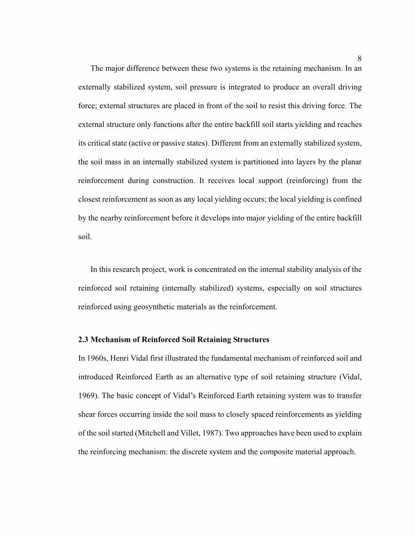
8The major difference between these two systems is the retaining mechanism. In an
externally stabilized system, soil pressure is integrated to produce an overall driving
force; external structures are placed in front of the soil to resist this driving force. The
external structure only functions after the entire backfill soil starts yielding and reaches
its critical state (active or passive states). Different from an externally stabilized system,
the soil mass in an internally stabilized system is partitioned into layers by the planar
reinforcement during construction. It receives local support (reinforcing) from the
closest reinforcement as soon as any local yielding occurs; the local yielding is confined
by the nearby reinforcement before it develops into major yielding of the entire backfill
soil.
In this research project, work is concentrated on the internal stability analysis of the
reinforced soil retaining (internally stabilized) systems, especially on soil structures
reinforced using geosynthetic materials as the reinforcement.
2.3 Mechanism of Reinforced Soil Retaining Structures
In 1960s, Henri Vidal first illustrated the fundamental mechanism of reinforced soil and
introduced Reinforced Earth as an alternative type of soil retaining structure (Vidal,
1969). The basic concept of Vidal’s Reinforced Earth retaining system was to transfer
shear forces occurring inside the soil mass to closely spaced reinforcements as yielding
of the soil started (Mitchell and Villet, 1987). Two approaches have been used to explain
the reinforcing mechanism: the discrete system and the composite material approach.

9The discrete system, shown in Fig.2.3.1, indicates that the additional shear forces of
the unstable soil mass are transferred to the reinforcement in two forms: friction and
adhesion. Friction is the component of shear resistance that is proportional to the normal
stress acting on the shear plane. Adhesion is the shear resistance between different
materials (soil and reinforcements) and is independent of normal stress (Hausmann,
1990). As a result of this internal shear transformation, the soil mass is kept away from
its critical state, and the lateral pressure that is generated by the reinforced soil mass is
also reduced because of the existence of the reinforcements.
The other approach to explain the reinforcing mechanism of reinforced soil is to
analyze it as a composite material. Schlosser and Long (1972) and Yang and Singh
(1974) used an apparent cohesion concept. Hausmann (1976) and Hausmann and Lee
(1976) also interpreted the reinforcing mechanism using similar concepts. Figure 2.3.2
summarizes the composite approach to the reinforcing mechanism using the
Mohr-Coulomb failure criteria (after Hausmann, 1990). As shown in Fig. 2.3.2, Mohr
circle 0 represents a reinforced soil composite element at its initial condition. Assume
that this element has reinforcement inserted in the horizontal plane, and a pair of
principal stresses (vertical and horizontal stresses, where vertical stress is the major
principal stress) are applied to it. When the vertical stress increases, the Mohr circle
moves to higher stress levels. Mohr circle 1 represents the failure condition if soil is not
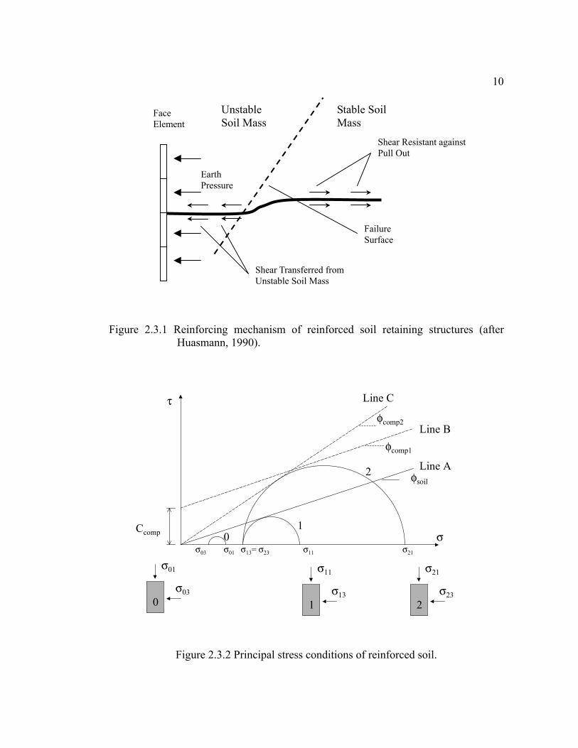
10
Figure 2.3.1 Reinforcing mechanism of reinforced soil retaining structures (after Huasmann, 1990).
Figure 2.3.2 Principal stress conditions of reinforced soil.
Unstable Soil Mass
Stable Soil Mass
Shear Resistant against Pull Out
Earth Pressure
Face Element
Shear Transferred from Unstable Soil Mass
Failure Surface
2
01
Line C
Line B
Line A
τ
σσ03 σ01 σ13= σ23 σ11 σ21
σ03
σ01
σ13
σ11
σ23
σ21
φsoil
φcomp1
φcomp2
0 1 2
Ccomp

11reinforced, and Mohr circle 2 represents the failure condition of the reinforced soil
composite. The difference between σ21 and σ11 is the additional vertical stresses that soil
can take with the aid of the reinforcement. Line A is the failure envelope of the
unreinforced soil. Lines B and C are two hypothetical failure envelopes that are used to
define the failure of the reinforced soil composite. Line B represents the hypothesis that
the reinforced soil composite has the same friction angle as the soil. What reinforcement
provides is an additional cohesion Ccomp to the composite. The hypothesis represented
by Line C is that the reinforced soil composite has higher friction angle because of the
existence of the reinforcement. Equations 2.3.1 and 2.3.2 are the equations of Lines B
and C, or
1compcomp tanC φ⋅σ+=τ (Line B) (2.3.1)
2comptan φ⋅σ=τ (Line C) (2.3.2)
Boyle (1995) verified that hypothesis presented by Line C (Equation 2.3.2) is more
appropriate to explain the reinforcing mechanism of GRS with his Unit Cell Device
(UCD) test data. The UCD was designed to test a GRS element under plane strain
loading conditions to simulate the GRS element inside GRS soil structures. Both in-soil
properties of geosynthetics and GRS composite properties are measured in the device
(Boyle, 1995). Boyle found that the tension that develops in the reinforcements during
straining of the GRS increased the lateral pressure acting on the soil, thus increasing the
soil strength.

12For failure mechanism of the GRS, Hausmann (1976), Hausmann and Lee (1976),
and Gray and Ohashi (1983) found that at low confining pressures, failure of reinforced
soil often occurred by slippage at the soil-reinforcement interface; and, at higher
confining pressures, failure occurred due to the rupture of the reinforcement. However,
this observation depends on the properties of the reinforcement material as well as the
interface between reinforcement and soil. The discrete system approach is suitable for
analyzing failure at both low and high confining pressures, although it involves
complicated force transformation. On the contrary, the composite material approach,
although less inter-layer force transformation is involved, will need a good constitutive
stress-strain model to account the very different behaviors of GRS composite at
different confining pressures.
2.4 Geosynthetic Reinforced Soil (GRS) Retaining Structures
Vidal’s Reinforced Earth system was constructed using horizontally lying steel strips as
reinforcement and with facing elements to locally retain the backfill soil. In addition,
different materials such as steel bars, wire mats, and synthetic fabrics have been used as
reinforcements for this system. Although its use as reinforcement did not start until the
early 1970’s, geosynthetics have become one of the most popular soil reinforcement
materials. The usage of geosynthetics for soil reinforcing has increased dramatically in
the past twenty years because (after Giroud, 1986):

131. Geosynthetic materials have excellent flexibility and uniformity, and therefore, they
have better tolerance of differential movements,
2. Geosynthetic materials are more resistant to corrosion and other chemical reactions
than steel reinforcement, and
3. Geosynthetic materials are able to provide the same (maybe even better) reinforcing
effect than the steel reinforcement with easier and more cost effective construction
procedures.
Despite considerable differences of reinforcing mechanisms, interaction with soil
and geosynthetics, and property changes due to in-soil confinement and low strain rate
conditions, stability analysis of GRS retaining walls is still performed in a similar
manner to that of steel reinforced retaining walls. Internal design methods adopted from
steel reinforced walls are based on limiting equilibrium concepts and require an
assumption of the lateral earth pressure distribution against the face of the reinforced
section in order to obtain the tensile stresses that must be resisted by the reinforcement.
Available evidence from full-scale and model GRS walls indicates that these
assumptions tend to significantly overestimate the internal stress distribution within the
structure (Bell et al., 1983; Rowe and Ho, 1993; Allen et al., 1992; Christopher, 1993).
These observations suggest that the assumptions of conventional lateral earth pressure
theory used in steel reinforced wall design is not appropriate for estimating the lateral
earth pressure distribution of GRS walls. To develop an appropriate internal stability

14design for GRS walls, an alternate approach to obtain the internal distribution of lateral
earth pressure behind the wall face is needed.
2.4.1 Reinforcing Mechanisms
The basic differences between steel and geosynthetic reinforcement are their stiffness,
structures, and the interactions occurring at the interfaces between reinforcement and
soil. Steel reinforcement is usually in the form of straps or mats (Fig. 2.4.1), while
geosynthetic reinforcement is usually in the form of grids or planar sheets (Fig. 2.4.2).
Because of the planar structure and flexibility of geosynthetics, the shear forces
occurring inside the soil mass are transferred to geosynthetic reinforcement more
uniformly and without interruptions; therefore, geosynthetic materials have a better
ability to contain both local and global yielding of the soil mass than steel reinforcement.
The limit equilibrium analysis assumes that reinforcement does not reinforce the soil
until global failure occurs in the soil mass. Although this analysis provides satisfactory
results for steel reinforced retaining structures, it tends to over-predict the internal stress
distribution of GRS retaining structures.
2.4.2 Interaction with Surrounding Soil
In contrast to the smooth surfaces that steel reinforcements usually have, most
geosynthetics have fabric-like surfaces (geotextiles) or grid structures (geogrids)

15
Figure 2.4.1 Examples of steel reinforcement: (a) steel straps, and (b) steel mats (Jones, 1996).
Figure 2.4.2 Examples of geosynthetic reinforcement: (a) geogrids, and (b) woven geotextile (Koerner, 1998).
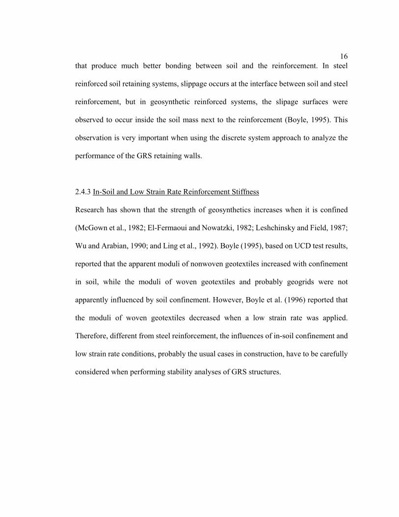
16that produce much better bonding between soil and the reinforcement. In steel
reinforced soil retaining systems, slippage occurs at the interface between soil and steel
reinforcement, but in geosynthetic reinforced systems, the slipage surfaces were
observed to occur inside the soil mass next to the reinforcement (Boyle, 1995). This
observation is very important when using the discrete system approach to analyze the
performance of the GRS retaining walls.
2.4.3 In-Soil and Low Strain Rate Reinforcement Stiffness
Research has shown that the strength of geosynthetics increases when it is confined
(McGown et al., 1982; El-Fermaoui and Nowatzki, 1982; Leshchinsky and Field, 1987;
Wu and Arabian, 1990; and Ling et al., 1992). Boyle (1995), based on UCD test results,
reported that the apparent moduli of nonwoven geotextiles increased with confinement
in soil, while the moduli of woven geotextiles and probably geogrids were not
apparently influenced by soil confinement. However, Boyle et al. (1996) reported that
the moduli of woven geotextiles decreased when a low strain rate was applied.
Therefore, different from steel reinforcement, the influences of in-soil confinement and
low strain rate conditions, probably the usual cases in construction, have to be carefully
considered when performing stability analyses of GRS structures.

172.5 Stability of GRS Retaining Structures
2.5.1 External Stability
All reinforced soil retaining walls, whether reinforced by steel or geosynthetics, have
the same external stability concerns as conventional retaining structures. Figure 2.5.1a
shows the external failure modes of GRS retaining structures. External stability design
of retaining structures basically includes analyses of:
1. Friction between retaining structures and foundation soil--possibility of base sliding
failure,
2. Bearing capacity of foundation soil and creep of the foundation soil--possibility of
overturning, and excessive settlement, and
3. Overall slope stability
2.5.2 Internal Stability
Figure 2.5.1b shows the internal failure modes and local stability failure modes of
segmental facing units. Different from the conventional system in which backfill soil
properties are the major internal stability design concern, the reinforced soil system has
a much more complicated internal stability design. Internal stability design of the
reinforced soil retaining structure involves consideration of:
1. The strength properties of backfill and reinforcement material,
2. The reinforcement arrangement,

18
Figure 2.5.1 Failure modes of segmental GRS retaining structures (after NCMA 1996).

193. Interaction between soil and reinforcement,
4. Interaction between facing element and soil,
5. Durability of the reinforcement, and
6. Connection between facing units and reinforcement (especially for systems with
segmental facing structures).
Present internal stability design methods of reinforced soil retaining structures are
still based on a limit state analysis. This approach fails to provide internal working
stress information as well as face deflections of the retaining structure. Furthermore, it
tends to over-predict the internal stress distribution inside GRS retaining structures
because of the considerable differences that were described in previous sections
between steel and geosynthetic reinforcements.
20Chapter 3
Internal Stability Analyses of GRS Retaining Structures
As summarized in Chapter 2, although improvement of the internal stability
analyses of GRS retaining structures is needed, previous research on this subject has
not made much progress because:
1. Minimal information on the internal stress or strain distributions in real GRS
structures is available. Because of the difficulties in installing appropriate
instrumentation to measure reinforcement strain and, most important, in
interpreting strain measurements obtained from the field, only a few reliable
internal stress or strain measurements are available.
2. Minimal calibration of numerical modeling techniques for analyzing the
performance of GRS walls has been done. Most of the time, numerical models
have been developed to simulate the performance of specific GRS retaining
structure projects. Parametric studies of the effect of internal design factors
have mostly been done by using models of hypothetical slopes or walls
generated by computer programs. Although some computer programs have
been used to perform numerical analyses on different GRS walls, procedures
for interpreting input properties were found to be unclear, or sometimes even
different procedures were used for models created using the same computer
program.

213. Understanding of material and interface properties is not well developed.
Within a GRS wall, material (both soil and geosynthetic) properties and the
interactions between them vary when the loading and confining conditions are
changed. Research on analyzing these material and interface changes has not
progressed very much because of difficulties in designing laboratory tests and
interpreting field measurements. Numerical analyses performed without
appropriate interpretation of input properties may yield reasonable results for
either external performance (face deflections) or internal performance
(reinforcement strain distributions), but not both at the same time.
To overcome these drawbacks, numerical models that use clear and reasonable
procedures to determine input material and interface properties as well as that are
capable of reproducing both the internal and external performance of GRS retaining
structures should be developed.
In this chapter, present internal stability design methods for GRS retaining
structures are reviewed and commented upon. A general review of previous numerical
modeling of GRS retaining structures is presented as well.
3.1 Concepts of Internal Stability Analyses of GRS Retaining Structures
Present internal stability analyses of GRS retaining structures basically consider two
reinforcement failure modes:

221. Rupture or excessive elongation in the high stress zone within the reinforced
backfill, and
2. Pull out or slippage from soil close to the end of the reinforced soil backfill.
However, stress or strain levels of the reinforced soil are not considered because
most of these analyses are based on limiting equilibrium concepts. In limiting
equilibrium analyses, the geosynthetic reinforcement is designed to be strong enough
to take all the excess earth pressure within the backfill soil; yet interaction between
soil and reinforcement, including force transformation, interlayer movements, and
other working stress mechanisms, are not considered.
Different from limiting equilibrium analyses, working stress analyses can provide
detailed internal and external stress-strain information of the structure. Information
such as the development of reinforcement tension and strain compatibility under
working conditions of the structure becomes available by performing working stress
analyses. However, working stress analyses of GRS retaining structures are difficult to
perform because limited calibration work of numerical modeling techniques has been
done and understanding of material and interface properties is not well developed.
In the following sections, concepts of both limiting equilibrium and working stress
analyses are described. The need for developing working stress based design methods
will be further confirmed.
23
3.1.1 Ultimate Limit State Stress Analysis
The ultimate limit state stress analysis is the most commonly used analysis method for
the stability of geotechnical projects such as retaining walls, slopes, excavations, as
well as foundation bearing capacity. Basic procedures of this type of analysis include:
1. Assume a reasonable collapse mechanism for the foundation.
2. Calculate the demand forces or moments for satisfactory performance of the
structure based on the assumed collapse mechanism. These forces or moments
become the ultimate limit state requirements of the designed structure.
3. Design resistant components that would provide enough resistant forces or
moments to the structure so that certain factors of safety (ratio of the resistant over
the demand forces or moments) can be achieved.
Advantages of ultimate limit state analysis are: (1) only simple calculations are
needed, and (2) results of the design tend to be on the conservative side, as long as the
assumed collapse mechanism is close to what really happens if the designed structure
collapses. However, the performance as well as the internal stress and strain levels of
the designed structure cannot be obtained from this type of analysis. For geotechnical
structures, such as GRS retaining walls with complicated interactions between
construction materials, as the difficulty of assuming a reasonable collapse mechanism
increases, the accuracy of calculating demand forces for design decreases. Therefore, a

24working stress analysis that can provide internal stress distribution as well as structure
performance becomes necessary.
3.1.2 Working Stress Analysis
Different from the ultimate limit state analysis, a working stress analysis analyzes the
actual stress levels within the designed structure. Basic procedures of a working stress
analysis include:
1. Develop analytical models for the elements (materials) that form the designed
structure and the interactions between them.
2. Calculate the stress and strain levels within the designed structure using
developed material and interface models based on laws of strain compatibility
and stress equilibrium.
3. Repeat the stress-strain calculation for each working stress condition that the
structure might experience.
Advantages of the working stress analysis are: (1) no assumption of a collapse
mechanism needs to be made, (2) the actual stress levels within the designed structure
can be obtained, and (3) the performance of the structure can also be observed.
However, analytical models for materials and interfaces between them are not always
easy to develop, and these types of analyses always involve complex equations and
numerous calculations. Numerical analysis methods such as finite element method or

25finite difference method are commonly used as tools to perform these types of
analyses.
In the remaining sections of this chapter, internal stability design methods of GRS
retaining structures based on both limit state analysis and working stress analysis are
reviewed. Technical problems of these methods and needs for developing general
rules and practical calculation methods for the working stress analysis of GRS
retaining structures will be summarized as well.
3.2 Internal Stability Analyses of GRS Retaining Structures I--Limit State Design
Methods
Allen and Holtz (1991), and Holtz et al. (1997) have summarized various internal
stability design methods. These methods are mostly based on ultimate limit state stress
analysis. General procedures for these methods include:
1. Assume a lateral stress (lateral earth pressure) distribution behind the wall
face.
2. Calculate reinforcement tension to avoid tensile failure of reinforcement based
on the assumed lateral earth pressure distribution with a certain factor of safety
applied.
3. Calculate required reinforcement length to avoid pull-out failure of the
reinforcement, based on the assumed lateral earth pressure distribution, failure

26plane orientation, and interlayer friction angle (soil-reinforcement) with certain
factor of safety applied.
A summary of these methods will be discussed in terms of assumed lateral earth
pressure distributions, determination of reinforcement tensile forces, and
determination of reinforcement embedment lengths required to resist pullout forces.
Only theoretical concepts are discussed in the following sections.
3.2.1 Lateral Earth Pressure Distributions
Several lateral earth pressure distributions have been proposed for internal stability
design for GRS retaining structures (Figures 3.2.1a to 3.2.1d). The most commonly
used is the classical Rankine earth pressure distribution, which assumes a triangular
shape lateral earth pressure distribution (Figure 3.2.1a). Use of the Rankine earth
pressure distribution was proposed by Steward et al. (1977), and is still extensively
used in many popular design methods such as FHWA (Federal Highway
Administration) (Holtz et al., 1997) and NCMA (National Concrete and Masonry
Association) (NCMA, 1996) methods.

27
γHKa 0.65γHKa
(a) Rankine (Triangular) (b) Rectilinear
γHKo γHKa
(c) Bilinear (d) Coherent gravity
Figure 3.2.1 Various lateral earth pressure distributions: (a) Classical Rankine (Triangular), (b) Rectilinear (Broms, 1978), (c) Bilinear (Christopher et. Al., 1989), and (d) Coherent gravity (Christopher et al. 1989, Simac et al. 1990).
2.35
6.1
Ko
Ka

28Other lateral earth pressure distributions such as rectilinear (Figure 3.2.1b, Broms,
1978), bilinear (Figure 3.2.1c, Christopher et al. 1989), and coherent gravity (Figure
3.2.1d, Christopher et al. 1989, Simac et al. 1990) distributions have been proposed.
These distributions were developed mostly based on field observations or experiences
to account for the soil-reinforcement composite effects. Leshchinsky and his
colleagues (Leshchinsky and Boedeker, 1989, Shiwakoti et al., 1998) also assumed a
triangular lateral earth pressure distribution for reinforcement tension calculations;
however, a logarithmic spiral failure surface was used to describe the failure
mechanism within the reinforced soil.
3.2.2 Reinforcement Tensile Forces
The Rankine earth pressure distribution does not take existing reinforcement
material properties into account when calculating the reinforcement tension at certain
heights of the wall. Additional adjustments of the lateral earth pressure coefficients
were made based on empirical experience when calculating the reinforcement tensions
(NCMA, 1996, Holtz et al, 1997).
In most of the limit state stress-based GRS internal stability analyses, concepts of the
tie-back wedge design method were adopted to calculate the reinforcement tensile
forces. In the tie-back method, the reinforcement was designed to resist the thrust that
resulted from the lateral earth pressure acting on the wall face in between the
29reinforcement layers. General procedures of this method are described in the following
sections.
Reinforcement tensile force at a certain depth from top of the wall is determined
by calculating the horizontal force at the same depth based on the assumed lateral
earth distribution (Equation 3.2.1). σh in Equation 3.2.1 is determined based on the
lateral earth pressure distribution used.
( ) ( ) vhinfre SzzT ⋅σ= (Eq. 3.2.1)
where Treinf (z) = reinforcement tensile force at depth z from top of the wall.
σh(z) = horizontal pressure at depth z from top of the wall.
Sv = vertical spacing of the reinforcement.
The calculated reinforcement tensile forces are then multiplied by a factor of
safety to use as the design reinforcement tensions (Equation 3.2.2). Different factors of
safety are used by different design methods because different lateral earth pressure
distributions or adjustments for existing reinforcement are used.
( ) ( ) FSzTzT infredesign ⋅= (Eq. 3.2.2)
where Tdesign(z) = designed reinforcement tension at depth z from top of the wall.
FS = factor of safety.

303.2.3 Reinforcement embedment length
The embedment length required to prevent pullout failure of the reinforcement is
calculated from force equilibrium at the depths where the reinforcement layers are
located. The resistant force against pullout failure is the friction developed on both
surfaces of the reinforcement, and the driving force is equal to horizontal force acting
on the plane where the reinforcement lies (Equation 3.2.3).
w1wL2f hrequired,e*
v ⋅⋅σ=⋅⋅⋅⋅σ (Eq. 3.2.3)
where σv = vertical earth pressure acting on the reinforcement.
f* = interlayer friction coefficient between soil and reinforcement.
Le, required = required embedment length of reinforcement.
w = unit width of the designed wall.
σh = horizontal earth pressure acting on the reinforcement.
σv in Equation 3.2.3 usually equals γ (unit weight) times z (depth) plus additional
surcharge loads, and σh can be determined using the assumed lateral earth pressure
distribution. By solving the force equilibrium described in Equation 3.2.3, the
designed reinforcement embedment length can be determined with an appropriate
factor of safety (Equation 3.2.4).
*v
hdesign,e f
12
FSL ⋅σσ⋅= (Eq. 3.2.4)

31where Le, design = design embedment length of reinforcement.
Values of minimum embedment length were also recommended in most of the
methods to prevent internal sliding between the geosynthetics and soil.
3.3 Analytical Models of Reinforced Soil
As described in Section 3.1.2, an important part of working stress analyses is to
develop analytical models for the materials used in GRS walls and the interfaces
between them. As described in Section 2.3, behavior of reinforced soil can be
analyzed using two approaches: the discrete soil reinforcement system and the
composite material model. Both approaches have been utilized to develop analytical
models for numerical analyses of GRS walls. Figure 3.3.1 describes the material
properties involved in both types of analytical models. The discrete element model
considers individual structural elements in the reinforced soil and the interfaces
between them, and the composite element model treats the reinforced soil as an
anisotropic homogeneous material. In the following sections, a review of these
analytical models and the numerical analyses developed based on them are described.
The progress and shortcomings of present research are summarized as well.

323.3.1 Discrete Element Model
The discrete element model analyzes individual structural elements of the reinforced
soil and interfaces between them (Figure 3.3.1a). Properties of the soil, reinforcement,
facing units, and interfaces between different materials are necessary to develop this
type of numerical model. An advantage of using the discrete soil-reinforcement
approach is that the stress levels in individual structural elements can be determined
within this model. Especially for segmental faced GRS retaining structures, important
design information such as friction between facing units and backfill, as well as
reinforcement stresses at the connections, can be estimated using this approach.
Disadvantages of this model are (after Rowe and Ho, 1988; Bathurst and Koerner,
1988):
1. Difficulty in developing numerical models--numerical models developed based on
this approach usually have many different material and interface elements
representing different materials and interfaces.
2. Difficulty of characterizing the interactions between soil, reinforcement and other
structural elements--input properties of interfaces between different materials in
the system are difficult to determine.
3. Large computation time required for the numerical analyses--numerical models
based on this approach usually require a large number of computation units
(elements), and the time required for numerical iterations is fairly large.

33
(a) discrete soil reinforcement model
(b) orthotropic elastic reinforced soil composite model.
Figure 3.3.1 Material properties involved in the development of the analytical models.
Soil (Mohr Coulomb Material)- E, modulus γ, unit weight φ, friction angleψ, dilation angle
Geosynthetic Reinforcement- J, stiffness
Ty, yield strengths Ae, contact area γ, unit weight
Interfaces between Soil and Geosynthetic Reinforcement- φ, friction
ks, shear stiffness kn, normal stiffness Py, yield limit
Orthotropic Elastic Reinforced Soil Composite- Mx, My, Mz, composite moduli
νxy, νyz, νzx, Poisson’s ratios of composite material
γ, unit weight of composite material
z
y
x

34So far, most of the working stress analyses for GRS retaining structures have been
performed using the discrete soil reinforcement system. Research progress and
difficulties encountered are summarized in Section 3.4.
3.3.2 Composite Element Model
The reinforced soil composite element model considers the reinforced soil to be an
anisotropic homogeneous material. As shown in Fig. 3.3.1b, only orthotropic elastic
composite material properties are needed to develop this type of numerical model.
Advantages of using the reinforced soil composite model are:
1. Less effort required to develop numerical models--by using composite material
concepts, only composite elements of reinforced soil are used in numerical
models; therefore construction of numerical models is much easier than using
discrete elements.
2. Less time needed for iterations--computation units (elements) of numerical models
are dramatically decreased by using the composite elements instead of different
material and interface elements, and the iteration time of a composite model is
expected to be much less than a discrete model that is modeling the same object.
Although the composite approach offers simpler and time saving numerical
analyses, yet it has following disadvantages (after Rowe and Ho, 1988):
351. Stress levels of individual structural materials are not available--the internal stress
or strain distribution is presented in a composite sense.
2. Interactions between different materials cannot be modeled--the composite model
assumes that reinforced soil has perfect bonding at the interfaces between soil and
reinforcement, interlayer movement such as slipages between soil and
reinforcement cannot be modeled.
3. Localized failure cannot be modeled--because no individual material elements are
used, localized failures such as connection failure of the segmental GRS walls
cannot be simulated.
Treating construction materials as composites has been proposed by, for example,
Westergaard (1938), Salamon (1968), Harrison and Gerrard (1972), Romstad et al.
(1976), and Shen et al. (1976). Among these researchers, Harrison and Gerrard (1972)
first applied the elasticity to analyze reinforced soil. They developed a series of
equations to convert individual elastic material properties into the elastic composite
material properties. The elasto-plastic model of reinforced soil composite was not
developed until 1980’s. Sawicki and Lesniewska (1988, 1991, 1993), and Sawicki and
Kulczykowski (1994) updated the elastic formulations to include plastic yielding of
the material. Effort has also been made to simulate the slip between soil and
reinforcement by adding extra yielding criteria into the composite elements (Hermann
and Al-Yassin, 1978; Naylor, 1978; Naylor and Richards, 1978).
36
The major difficulty in performing numerical analyses using composite elements is
obtaining the composite properties of the reinforced soil. In the present research,
composite material properties were first interpreted from individual material properties
using developed elasticity models; thus numerical analyses were performed using the
interpreted composite material properties. Boyle (1995) developed the Unit Cell
Device (UCD) to test reinforced soil composites under plane strain loading conditions.
Anisotropic composite properties were obtained by reducing the UCD test data (Lee
and Holtz, 1998). These composite properties were also used as the input properties of
numerical models that were developed to simulate the WSDOT Rainier Avenue wall
performance. These models were able to predict the wall performance reasonably well
(Lee and Holtz, 1998).
3.4 Internal Stability Analyses of GRS Retaining Structures II--Working Stress
Design Methods and Numerical Analyses
3.4.1 Present Working Stress Design Methods
So far, working stress analyses for both performance and internal stability designs of
GRS retaining structures are not well developed. Existing case histories utilizing
working stress analyses were done by numerical techniques. Numerical models were
created using various finite element or finite difference computer programs to either
examine designs for critical structures or reproduce instrumentation measurement for
research purposes. However, performance prediction of any large-scale test walls or
37real walls has not previously succeeded using working stress analyses. Major reasons
for this is the lack of knowledge of in-soil geosynthetic properties, strain rate-
dependent geosynthetic properties, and soil-geosynthetic interface mechanisms.
Arbitrary assumptions of material properties were involved in most of these models;
i.e. determination of input properties often changed when different objects were
analyzed.
Recently, a commercial finite difference method (FDM) based computer program
FLAC has become popular for analyzing geotechnical stability problems. Numerical
models of GRS retaining structures have been developed using FLAC by several
researchers, including the author. With aid of recent progress in understanding of
material properties, these models were able to reproduce the performance of different
GRS retaining structures even using the same procedures to determine material
properties and to model the interaction between soil and geosynthetic.
3.4.2 Summary of Numerical Analysis Methods
Both the finite element method (FEM) and the finite difference method (FDM) were
used to perform working stress analyses to predict performance of GRS retaining
structures. Various computer programs have been developed using both the discrete
and composite approaches. In this section, both FEM and FDM methods are reviewed,
and problems encountered and progress are summarized.
383.4.2.1 Finite Element Method
Table 3.4.1 summarizes some of the popular FEM computer programs and researchers
that have used these programs as tools to perform numerical analyses on GRS
retaining structures. Although a lot of FEM computer programs have been used to
model the performance of GRS retaining structures, none of them have really
succeeded because of the difficulties described at the beginning of this chapter.
Problems in modeling GRS retaining structures include:
1. Both internal and external performance cannot be accurately predicted at the
same time.--Because of inadequate consideration of in-soil and low strain rate
strength properties of geosynthetic reinforcement, results of these FEM
analyses could often only match either wall deflections or reinforcement
stress/strain levels, and not both at the same time.
2. Adjustments to input material properties were made without a clear
explanation or consistent rules.--In order to make an accurate prediction of
both internal and external performance, some of these analyses had to apply
different “in-soil” stiffness adjustments for geosynthetic reinforcement for
different modeling projects.
3. The result of parametric analyses cannot be correlated to real wall
performance.--Although some parametric studies of design factors of GRS
retaining structures have been performed using these FEM programs, results of

39these studies did not correlate very well to real wall performance. One of the
major reasons for this poor agreement is that most of the parametric studies
were done using hypothetical models that were still having the problems
described above.
4. Another problem of using the FEM programs to model GRS retaining
structures is that most of these programs were developed for research purposes.
Modeling techniques such as the determinations of input material or interface
properties were often changed when different projects were analyzed.
Table 3.4.2 summarizes the problems found in modeling performance of GRS
retaining structures using the FEM computer programs listed in Table 3.4.1.
3.4.2.2 Finite Difference Method
Recently, the FDM program FLAC has become popular for modeling the
performance of GRS walls because of its excellent capability to model geotechnical
engineering stability problems and its extended programming ability (Itasca, 1995).
Besides research results presented in this thesis, Bathurst and Hatami (1998a and b)
have used the FLAC program to analyze the seismic response of GRS walls. They also

40Table 3.4.1 FEM programs used to analyze performance of GRS retaining structures.
Program Names References
REA
Herrmann and Al-Yassin (1978) Xi (1992)
SSCOMP
Seed and Duncan (1984) Collin (1986) Adib (1988) Schmertmann, et al. (1989) Chew, et al. (1989) Jaber, et al. (1992) Zornberg and Mitchell (1993) Chew and Mitchell (1994) Pinto, et al. (1998)
AFENA
Ho and Rowe (1993) Ho and Rowe (1994)
DACSAR
Chou (1992) Helwany (1992) Chou and Wu (1993)
SOILSTRUCT
Ebling, et al. (1992a) Ebling, et al. (1992b) Ebling, et al. (1993)
GEOFEM
Karpurapu and Bathurst (1992) Karpurapu and Bathurst (1994) Bathurst, et al. (1997)
CRISP
Yeo, et al. (1992) Andrawes and Saad (1994) Yogarajah and Andrawes (1994) Ghinelli and Sacchetti (1998)
M-CANDE
Ling and Tatsuoka (1992) Porbaha and Kobayashi (1997)
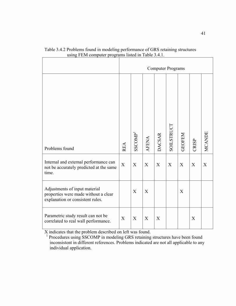
41
Table 3.4.2 Problems found in modeling performance of GRS retaining structures using FEM computer programs listed in Table 3.4.1.
Computer Programs
Problems found REA
SSC
OM
P1
AFE
NA
DA
CSA
R
SOIL
STR
UC
T
GEO
FEM
CR
ISP
MC
AN
DE
Internal and external performance can not be accurately predicted at the same time.
X
X
X
X
X
X
X
X
Adjustments of input material properties were made without a clear explanation or consistent rules.
X
X
X
Parametric study result can not be correlated to real wall performance.
X
X
X
X
X
X indicates that the problem described on left was found. 1 Procedures using SSCOMP in modeling GRS retaining structures have been found
inconsistent in different references. Problems indicated are not all applicable to any individual application.
42performed parametric studies to examine the influence of various internal design
factors. The numerical interpretation models that Bathurst and Hatami (1998a and b)
used were hypothetical models. These models were not calibrated using any actual
wall performance or large-scale test results. Lindquist (1998) also used FLAC to
analyze the seismic response of GRS slopes. A parametric study of seismic design
factors was performed using the developed model, and test results of centrifuge model
tests under dynamic shaking were reproduced (Lindquist, 1998). Adjustments to soil
and in-soil reinforcement properties without a clear explanation and verification were
found in the models developed by Lindquist (1998). Different values of soil friction
angle and reinforcement stiffness had to be systematically introduced into his models
in order to match the results of centrifuge and shaking table tests. FLAC models
described in these references were all created using discrete elements.
3.5 Conclusions
3.5.1 Problems of Present Numerical Analysis Applications
1. Present FEM programs have difficulties to predict both external and internal
performance data of GRS retaining structures at the same time. Although some of
them reported that successful modeling results had been obtained for both internal
and external performance, adjustments of the input material properties had to be
made, often without clear explanation.

432. Input properties used in some numerical methods are still decided based on
personal experience or, most of the time, arbitrary assumptions. Present numerical
analyses are usually performed by systematically introducing different values of
soil friction angles, soil dilation angles, or reinforcement stiffnesses. Specific
procedures that take material properties from laboratory test results and convert to
input parameters for numerical analyses are not well developed yet.
3. Numerical models developed using FLAC program have not been well calibrated
with real wall performance.
3.5.2 Research Needs for Internal Stability Analyses of GRS Retaining Structures
To improve the numerical analyses of internal stability of GRS retaining structures,
research is needed to:
1. Develop simple and straightforward procedures for converting material properties
that are obtained from ordinary laboratory tests to properties of materials that are
really present inside GRS retaining structures. Two examples are to convert a
triaxial soil friction angle into a plane strain soil friction angle, and to convert in-
isolation tensile properties to in-soil tensile properties of reinforcements.
2. Develop general rules (techniques) for numerical modeling that are capable of
predicting both internal and external performance using input properties that have
real physical meaning.

44
3. Perform parametric studies on these internal design factors using well calibrated
numerical models to obtain a better understanding of the influence of these design
factors.

45Chapter 4
Elasticity Theory and Stress-Strain Interpretation Used to Develop
the GRS Composite Model
4.1 Elasticity
This chapter describes the fundamental elasticity theory and stress-strain interpretation
used to develop the GRS composite model.
4.1.1 Transversely Isotropic Elasticity
Real soil is seldom an isotropic material. In most cases, soil responds in the same way
if it is loaded in any horizontal direction, and may respond differently if it is loaded in
the vertical direction. The behavior of soil is similar to the behavior of a transversely
isotropic material (Wood, 1990). Transversely isotropic materials have the same
stress-strain relationships in two of the three principal directions. Especially for the
reinforced backfill of retaining structures, horizontally layered reinforcements and
uniform backfill material make this soil-reinforcement “composite” a typical
transversely isotropic material.
Equation 4.1.1 shows the complete description of an orthotropic elastic material.
In Eq.4.1.1, E1, E2, E3, µ12, µ23, µ31, ν32, ν23, ν13, ν12, ν21, and ν31 are defined as the
elastic moduli, shear moduli and Poisson’s ratios of the anisotropic elastic material in
its three principal directions (Figure 4.1.1).
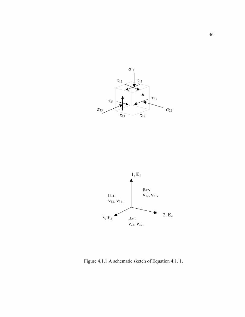
46
Figure 4.1.1 A schematic sketch of Equation 4.1. 1.
1, E1
2, E2 3, E3
µ12, ν12, ν21, µ31,
ν13, ν31,
µ23, ν23, ν32,
σ22
σ11
σ33
τ13
τ23
τ12
τ12
τ23
τ13
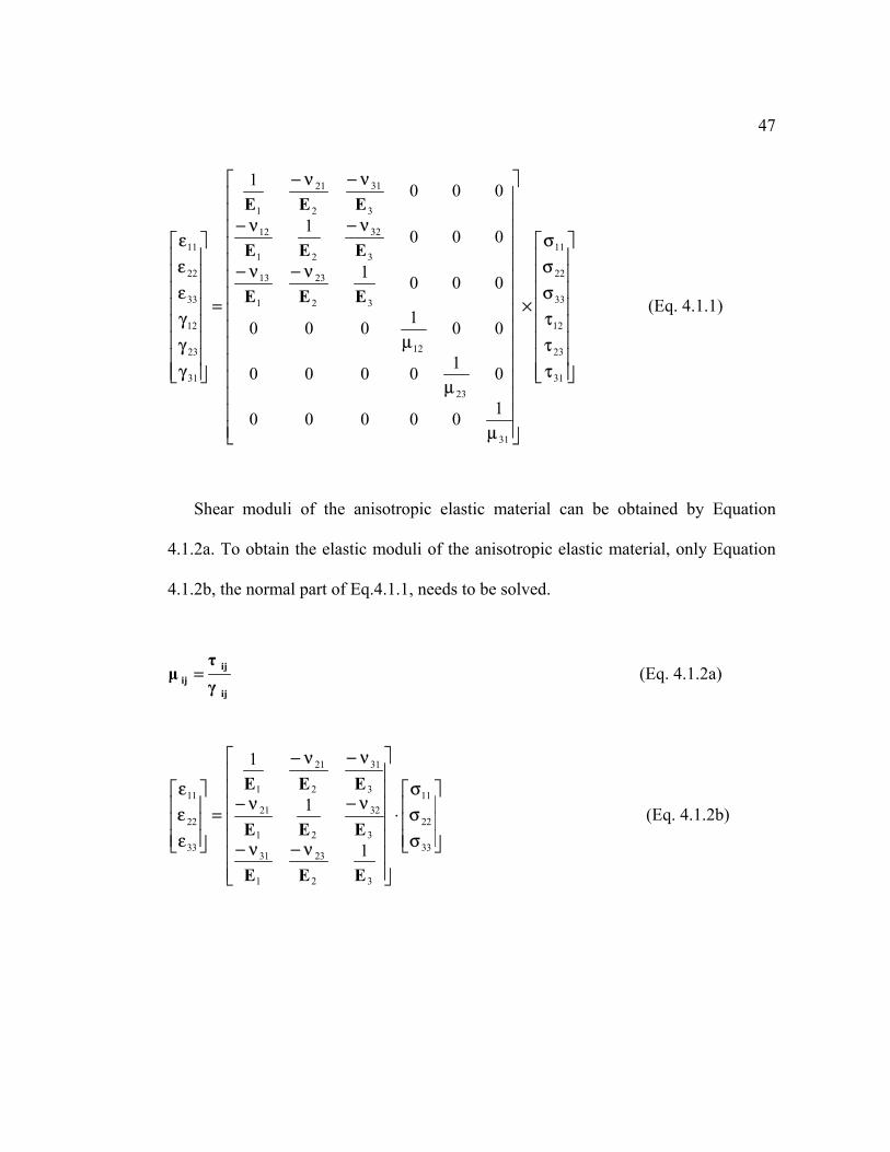
47
τττσσσ
×
µ
µ
µ
ν−ν−
ν−ν−
ν−ν−
=
γγγεεε
31
23
12
33
22
11
31
23
12
32
23
1
13
3
32
21
12
3
31
2
21
1
31
23
12
33
22
11
100000
010000
001000
0001
0001
0001
EEE
EEE
EEE
(Eq. 4.1.1)
Shear moduli of the anisotropic elastic material can be obtained by Equation
4.1.2a. To obtain the elastic moduli of the anisotropic elastic material, only Equation
4.1.2b, the normal part of Eq.4.1.1, needs to be solved.
ij
ijij γ
τµ = (Eq. 4.1.2a)
σσσ
⋅
ν−ν−
ν−ν−
ν−ν−
=
εεε
33
22
11
32
23
1
31
3
32
21
21
3
31
2
21
1
33
22
11
1
1
1
EEE
EEE
EEE
(Eq. 4.1.2b)

48By assuming the material transversely isotropic, and the major principal stress acts
in the vertical direction, E1 =Ev, E2 =E3 =Eh, ν32 = ν23 =νhh, ν31 = ν21 =νhv, and ν13 =
ν12. =νvh into Equation 4.1.2b, it can be further simplified as Equation 4.1.3.
σσσ
⋅
ν−ν−
ν−ν−
ν−ν−
=
εεε
33
22
11
33
22
11
1
1
1
hh
hh
v
vh
h
hh
hv
vh
h
hv
h
hv
v
EEE
EEE
EEE
(Eq. 4.1.3)
4.1.2 Plane Strain Loading Conditions
For the material elements inside soil structures like retaining walls, long
embankments, or slopes, it is appropriate to apply plane strain loading conditions to
analyze their stress-strain behavior. Plane strain conditions indicate that there is no
strain in one of the horizontal direction, for example, if direction 2 is the plane strain
direction, then ε22 = γ12 = γ23 = 0. Figure 4.1.2 shows a material element under plane
strain loading condition. Equations 4.1.4 and 4.1.5 are expanded from Equation 4.1.3
for plane strain. These two equations and Equation 4.1.6, the shear part, therefore
represent the transversely isotropic elasticity model for a material element under plane
strain loading conditions.
hhh
hvvh EEE
33221122 0
σν−
σ+
σν−==ε (Eq. 4.1.4)
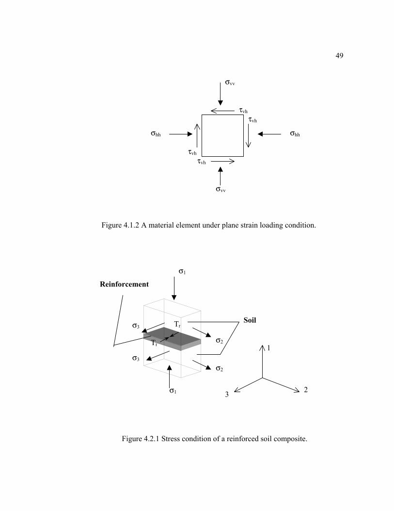
49
Figure 4.1.2 A material element under plane strain loading condition.
Figure 4.2.1 Stress condition of a reinforced soil composite.
σ1
σ1
σ3
σ3
σ2
σ2
Tr
TrSoil
Reinforcement
1
2 3
σvv
τvhτvh
τvhτvh
σvv
σhh σhh

50
σσ
⋅
ν−
νν−ν−
νν−ν−
ν−
=
εε
33
112
2
33
11
1
1
h
hh
hh
hhhvhv
h
hhhvhv
h
hv
v
EEE
EEE (Eq. 4.1.5)
31
3131 γ
τµ = (Eq. 4.1.6)
4.2 Stress-Strain Interpretations of a GRS Composite Element
The elasticity theories described in the previous section are only for homogeneous
materials. To apply them to obtain moduli of composite materials, composite stresses
and strains have to be used in Eqs. 4.1.4 and 4.1.5. In this research, the developed
GRS composite model was applied to the UCD test data. A UCD specimen is exactly
a reinforced soil composite element under plane strain loading condition (Fig. 4.2.1).
In order to obtain the reinforced soil composite moduli, measurements of stresses σ1,
σ2, and σ3, and reinforcement tension, Tr have to be interpreted into composite
stresses.
As shown in Fig. 4.2.1, pressure σ1 is the stress applied to the composite element
in direction 1. Instrumentation was used to measure the soil stresses σ2 and σ3, and the
reinforcement tension, Tr. Pressure σ1 and strain in direction 1 are the stress and strain
that the reinforced soil composite element has in direction 1 (Eq. 4.2.1).

51
1comp1 σ=σ , 1comp1 ε=ε (Eq. 4.2.1)
where ε1 = the strain of the composite element in direction 1
Direction 2 is the direction that controls the plane strain condition; i.e. there is no
strain in direction 2 and the reinforcement tension in that direction is negligible.
Therefore, measured pressure σ2 and strain in direction 2 also can be used as the stress
and strain of reinforced soil composite element in direction 2 (Eq.4.2.2).
2comp2 σ=σ , 2comp2 ε=ε (Eq. 4.2.1)
where ε2 = the strain of the composite element in direction 2
In direction 3, because uniform deformation is controlled, the composite stress can
be defined as:
3
3comp3 A
F=σ
where G3S33 AAA += , A3G and A3S are the areas of the reinforcement and the
soil element in direction 3, and
rS333 TAF +⋅σ= , total force in direction 3
Because A3S >> A3G, S33 AA ≈ . Therefore stress and strain in direction 3 for the
reinforced soil composite are:
52
3
r3comp3 A
T+σ=σ (Eq. 4.2.3)
3comp3 ε=ε (Eq. 4.2.4)
where A3 = the area of the composite element in direction 3
ε3 = the strain of the composite element in direction 3
Equations 4.2.1 to 4.2.4 were used in this research to convert the UCD test data
into composite stress and strain information. The composite stress and strain
information were introduced into the transversely isotropic material model to solve the
composite strength properties of reinforced soil composite (Lee and Holtz, 1998).

53Chapter 5
Research Objectives
Objectives of this research include:
1. Develop numerical techniques that are capable of analyzing the performance of
GRS retaining structures--Numerical GRS wall models that are able to provide
information on the internal stress-strain distribution and external wall performance
will be developed.
2. Verify the numerical modeling techniques--To verify the developed numerical
modeling techniques, numerical models of GRS retaining structures will be
created, and results will be compared to the field instrumentation measurements.
3. Perform parametric studies on internal design factors--The internal stability design
factors such as layer spacing, strength properties of geosynthetic reinforcement,
and facing stiffnesses will be used as the controlling factors in the parametric
studies. The parametric studies will investigate the influence of these design
factors on the performance GRS retaining structures.
4. Develop a composite method for internal stress-strain analysis--A composite
analytical method that analyzes the stress-strain behavior of GRS in a composite

54material concept. Composite strength properties will be obtained by reducing UCD
test data and then used as input properties for the composite numerical models of
GRS retaining structures.
5. Provide recommendations for improving internal design procedures for GRS
retaining structures--At the end of this research, recommendations for improving
the internal stability design procedures of GRS retaining structures will be
provided.

55Chapter 6
Scope of Work
Specific tasks to accomplish the research objectives are outlined in the following
paragraphs.
6.1 Development of Numerical Techniques for Analyzing GRS Retaining
Structure Performance
The first task of this research was to develop general “rules” (modeling techniques)
for performing working stress analyses when utilizing numerical techniques to analyze
the performance of GRS retaining structures. In this research, numerical techniques
were developed to create models of GRS retaining structures. By using these
numerical models, the performance of GRS retaining structures was analyzed. The
finite difference computer program, FLAC, was used to develop the numerical models
of GRS retaining structures. Numerical models were first created for a 12.6 m high
wrapped face GRS wall, the Rainier Avenue wall built in Seattle, Washington. This
FLAC model was able to accurately reproduce field instrumentation measurements,
and techniques of numerical modeling such as determination of input properties,
installation of boundary conditions, and FLAC programming were also developed.
Detailed modeling techniques developed in this research are described in Chapter 8.
Results of this modeling work are given in Chapter 9.

566.2 Verification of the Developed Modeling Techniques
In order to verify the developed numerical modeling techniques, FLAC models of
other GRS retaining structures were also created using the same modeling techniques
developed in the previous task. These models were developed to predict performance
of other case histories and large scale model tests as well. Purpose of this task was to:
1. Calibrate the modeling techniques using case histories,
2. Update the modeling techniques, and
3. Predict the performance of large scale GRS model wall tests.
6.2.1 Calibration of the Modeling Techniques Using Case Histories
Performance data from a few instrumented GRS retaining structures, including three
concrete panel walls, a modular block faced wall, and a wrapped faced wall of the test
walls constructed at the FHWA Reinforced Soil Project site at Algonquin, Illinois,
were obtained for this task. These performance data were reproduced using the
developed modeling techniques. Purpose of this task was to calibrate the developed
modeling techniques so that they can be universally applicable.
6.2.2 Update of the Modeling Techniques
Additional modeling techniques were developed when different structures were
analyzed, such as those with different facings, different boundary conditions, and
different types of surcharging. Models of Algonquin test walls were developed in this

57task for developing modeling techniques of wall cases other than wrapped face walls.
Modeling techniques have been updated during this task.
6.2.3 Predict the Performance of Large Scale GRS Model Wall Tests
To further verify the developed modeling techniques, numerical models of some large-
scale GRS model walls were created. These large-scale GRS model walls were built
and tested at the Royal Military College of Canada (RMCC). Large-scale GRS walls
tested in laboratory provide advantages of more uniform material properties, better
instrumentation measurements, incremental surcharge loading, and simpler boundary
conditions. Instrumentation measurements of three large-scale model test walls that
were designed to systematically change the internal stability design factors such as
layer spacing and reinforcement stiffness were modeled. Class A predictions,
predictions made before the completion of wall construction, were performed on two
of the test walls to demonstrate the feasibility of the developed modeling techniques.
Modeling techniques for determination of material and interfaces properties, and
installation of boundary conditions, were further examined. Appropriate adjustments
to the modeling techniques and material properties were again made to improve the
utility and accuracy of the numerical models of GRS retaining structures.
586.3 Parametric Study on the Internal Design Factors
Another important task of this research was to examine the influence of the internal
design factors on the performance of GRS retaining structures. A parametric study
was performed on the internal design factors such as layer spacing, ratio of
reinforcement length to wall height, soil strength properties, reinforcement strength
properties, and facing types.
Two types of parametric analyses were performed in this research. In first type,
numerical models developed in previous tasks for modeling the performance of the
Rainier Avenue wall and the Algonquin FHWA concrete panel test walls were used as
the fundamental models of the parametric study. Major internal stability design factors
were systematically introduced into the models. The analyses were performed by
varying only one design factor in each group while the other factors were fixed.
The second type of parametric study was performed using a large amount of GRS
wall models with different internal stability design factors. Design factors such as
layer spacing, soil strength properties, and reinforcement properties were
systematically introduced into these models to observe combination effects of design
factors.
Hypothetical GRS wall performance factors such as internal stress-strain levels
and face deformations were recorded and analyzed in both types of parametric

59analyses. The purpose of the parametric study was to obtain a thorough understanding
of the influence of the major internal stability design factors on the performance of
GRS retaining structures. With a better understanding of the internal design factors,
the internal stability analysis and design of the GRS retaining structures are expected
to be improved.
6.4 Composite Method for Working Stress-Strain Analysis
In this research, effort was also made to develop a composite method to analyze the
stress-strain behavior of the GRS element as well as the performance of GRS retaining
structures. The purpose of this part of research was to evaluate the feasibility of using
the composite approach to access the working stress-strain information in GRS
retaining structures. Moreover, in a real design project, time and cost might limit
performing complicated numerical analyses such as developing discrete numerical
models. The composite method for a working stress analysis could offer a time saving
access to working stress-strain information for preliminary investigations and design if
sufficient composite GRS properties were available.
An analytical model that treats the GRS composite as a transversely isotropic
homogenous material was developed. This analytical model was then used to reduce
GRS composite test data obtained from UCD test results (Boyle, 1995) to obtain the
composite properties of GRS. Composite numerical models were then developed
using composite GRS properties as the input properties. Since the composite GRS

60properties are the only inputs for the composite numerical models, less computation
time and iteration processes are expected. Moreover, information on the anisotropy of
internal stress distributions of GRS retaining structures was obtained from the results
of the composite numerical models as well.
6.5 Improvement of GRS Retaining Wall Design
The development of a practical and accurate design procedure for GRS retaining
structure systems was the most important objective of this research. Improved
knowledge of the influence of various design factors obtained from the previous tasks
was utilized to develop an improved design procedure and performance prediction
method for GRS retaining structures. Included was detailed information on modeling
techniques, which include determination of soil and geosynthetic properties,
determination of properties of interfaces between different materials, and FLAC
programming as well.
In the following chapters, the results of the research conducted to meet the stated
objectives are presented. Chapter 7 describes the determination of the material
properties of GRS retaining structures, while Chapter 8 describes the FLAC
techniques used for modeling the performance of GRS retaining structures. Chapter 9
describes the modeling results of existing GRS wall case histories, and Chapter 10
presents the predictions of the performance of the large scale walls tested in the
laboratory.

61
Analytical models used in the parametric analyses are given in Chapter 11, while
Chapter 12 presents the results of an extensive parametric study of the internal design
factors of GRS walls. Chapter 13 gives a new anisotropic model of GRS composites
and its application to perform prediction of GRS retaining structures. Performance
prediction methods and design recommendation for GRS retaining structures are
presented in Chapter 14, and finally the summary, conclusions, and future research
suggestions are presented in Chapter 15.
62Chapter 7
Material Properties in GRS Retaining Structures
Successful working stress analyses rely very much on a good understanding of input
material properties. Material properties under working conditions must be carefully
investigated before performing working stress analyses. Construction materials of
GRS retaining structures include backfill soil, geosynthetic reinforcement, and facing
units, if any. Properties of these materials vary when different loading, deformation, or
confinement conditions are applied. For example, properties such as the friction angle
and the elastic modulus of a soil change when different loading conditions are applied;
stiffnesses of geosynthetics are affected by the strain rate as well as by confinement.
In this chapter, properties of construction materials under loading conditions that
occur inside GRS retaining structures are discussed, and the appropriate selection of
these properties for numerical models is described.
7.1 Soil Properties
For soil structures such as retaining walls, long embankments, or slopes, it is
appropriate to represent the conditions inside these structures using plane strain
loading conditions. Recent GRS retaining structure analyses has also suggested that
plane strain soil properties should be used when analyzing the behavior of
geosynthetic reinforced walls (Rowe and Ho, 1993; Bathurst, 1993; and Zornberg et

63al., 1998). Plane strain strength properties of soil such as friction angle and elastic
modulus are different from those properties obtained from traditional soil strength
tests such as triaxial and direct shear tests.
Another major concern of soil properties inside GRS retaining structures is the
confining pressure. The lateral earth pressure range for retaining walls is relatively low
compared to the range of confining pressures that has been commonly reported in soil
strength test data. As shown in Table 7.1.1, the typical lateral earth pressure range for
walls with heights lower than 10m is only 0 to 100 kPa. Yet very few soil tests have
been conducted with confining pressures less than 100kPa.
Effort has been made in this research to characterize the low confining pressure
plane strain soil properties, in order to perform accurate working stress analyses of
GRS retaining structures. In the following sections, the differences between plane
strain loading conditions and triaxial loading conditions are first described. Results of
both plane strain and triaxial tests that were performed at low confining pressures are
compared. Applications of low confining pressure plane strain soil properties will be
discussed as well.

64
Table 7.1.1 Typical earth pressure range for walls with heights less than 10m. Depth from top of
the wall (m)
Overburden pressurea
(kPa)
Lateral earth pressure, at restb
(kPa)
Active lateral earth pressurec
(kPa) 1 20 10 6
2 40 20 12
3 60 30 18
4 80 40 24
5 100 50 30
6 120 60 36
7 140 70 42
8 160 80 48
9 180 90 54
10 200 100 60 a unit weight of soil was assumed to be 20 kN/m3. b lateral earth pressure coefficient at rest was assumed to be 0.5 (φ = 30 deg) c active lateral earth pressure coefficient was assumed to be 0.3 (φ = 30 deg)
657.1.1 Plane Strain Loading Conditions
Plane strain conditions mean that there is no strain in one of the principal directions.
For retaining walls, usually the direction parallel to the wall face is assumed to be the
direction without strain (or displacement).
Figure 7.1.1 shows a material element under plane strain loading conditions.
Compared to a material element under triaxial loading conditions, one of the common
loading conditions of soil testing (Figure 7.1.2), there is more confinement in the
horizontal directions in plane strain. Plane strain strength properties of soil such as
friction angle, cohesion, and elastic modulus should be investigated in order to have
accurate material information when performing working stress analyses.
7.1.2 Plane Strain Soil Test Results
In this section, plane strain test results for Ottawa sand and two different granular soils
that were the backfill materials of the GRS wall case histories analyzed in this
research are presented. Table 7.1.2 presents the prepared density, relative density, and
plane strain test device used with these three test materials. Figure 7.1.3 shows the
grain size distributions of these three soils.
The plane strain test results of these three soils were also compared to their triaxial
test results. The comparison is concentrated on cases in which confining pressures are
lower than 100 kPa because, as stated in the beginning of this section, 0 to 100 kPa

66
Figure 7.1.1 A material element under plane strain loading conditions.
Figure 7.1.2 A material element under typical triaxial loading conditions.
σ1, ε1
σ1, ε1
σ2 = σ3 ε2 = ε3
σ2 = σ3
ε2 = ε3
σ1, ε1
σ1, ε1
σ3, ε3
σ3, ε3 σ2 ε2 = 0
σ2 ε2 = 0

67
Table 7.1.2 Descriptions of soils tested under plane strain loading conditions. Name Description Tested Densitya
(Relative density) Plane Strain Test Device
Ottawa Sand Rounded, uniformly graded,
17.0 kN/m3 (90%)
UCD (Boyle, 1995)
Rainier Sand Angular, poorly graded, (Backfill material of the WSDOT Rainier Avenue geotextile wall, Seattle, Washington)
18.0 kN/m3
(90%)
UCD (Boyle, 1995)
RMC sand Sub-angular to angular, poorly graded, (Backfill material of large scale test walls tested at Royal Military College of Canada, Kingston, Ontario)
16.4 kN/m3
(50%)
UC Berkeley plane strain test device (Riemer, 1999)
a average density of all specimens tested
Figure 7.1.3 Grain size distributions of three tested soils.
0
10
20
30
40
50
60
70
80
90
100
0.01 0.1 1 10
Grain Size (mm)
Perc
ent P
assi
ng (%
)
Rainier Sand
RMC SandOttawa Sand

68 would be the appropriate lateral earth pressure range for common retaining walls
(with heights lower than 10m). Initial moduli, 1% strain secant moduli, and friction
angles obtained from both plane strain and triaxial tests were evaluated. The 1% strain
secant moduli were chosen because most of the analyzed cases histories showed an
average working strain about 1%. Values of the soil initial moduli, 1% strain secant
moduli, and friction angles were obtained by analyzing the test data.
Figure 7.1.4 shows the plane strain test results of Ottawa sand (Boyle, 1995).
Compared to the triaxial test results shown in Figure 7.1.5a, the plane strain initial
moduli were higher about 40% to 80% than the triaxial initial moduli at the confining
pressure range tested (less than 100 kPa); yet much less difference was found in the
1% secant moduli for 25 and 50 kPa (Table 7.1.3). Soil friction angles obtained from
both plane strain and triaxial tests were very similar (Table 7.1.3).
Figures 7.1.6 and 7.1.7 show the plane strain and triaxial test results respectively
of Rainier sand. This sand is more angular than Ottawa sand and was prepared at a
high relative density of 90%. Initial moduli obtained from plane strain tests were
found to be about seven to eight times the initial moduli obtained from triaxial tests.
The 1% strain secant moduli obtained from plane strain tests were about 100% higher
than those obtained from triaxial tests at confining pressures lower than 75kPa. Soil
friction angles obtained from plane strain tests were also higher than those obtained
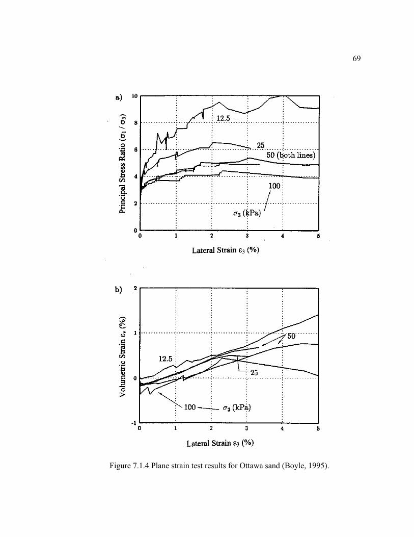
69
Figure 7.1.4 Plane strain test results for Ottawa sand (Boyle, 1995).

70
Figure 7.1.5 Triaxial test results for Ottawa sand (Boyle, 1995).

71
Table 7.1.3 Summary of strength properties of Ottawa sand.
Test Condition (confining pressures)
Initial Modulus,
(kN/m2)
1% Strain Secant Modulus, (kN/m2)
Friction Angle1,
(deg) 25 kPa 3.5E+4 1.45E+4 47 Plane
Strain 50 kPa 4.0E+4 2.2E+4 42
25 kPa 2.0E+4 1.3E+4 45 Triaxial
50 kPa 2.8E+4 2.2E+4 42 1 Calculated using equation φ = Sin-1[(Sr-1)/(Sr+1)], where Sr = (σ1/σ3) at peak.

72
Figure 7.1.6 Plane strain test results for Rainier sand (Boyle, 1995).

73
Figure 7.1.7 Triaxial test results for Rainier sand (STS, 1990).

74
Table 7.1.4 Summary of strength properties of Rainier sand.
Test Condition (confining pressures)
Initial Modulus,
(kN/m2)
1% Strain Secant Modulus, (kN/m2)
Friction Angle1,
(deg) 25 kPa 1.2E+5 3.0 E+4 59
50 kPa 2.5 E+5 4.25 E+4 56
Plane Strain
75 kPa 3.5 E+5 6.0 E+4 55
25 kPa 1.8 E+4 1.4 E+4 49
50 kPa 3.0E+4 2.5 E+4 47
Triaxial
75 kPa 4.2 E+4 3.3 E+4 47 1 Calculated using equation φ = Sin-1[(Sr-1)/(Sr+1)], where Sr = (σ1/σ3) at peak.

75from triaxial tests (Table 7.1.4). Test results shown in Figures 7.1.6 and 7.1.7 also
indicated that, for dense angular materials, the soils tested under plane strain loading
conditions tended to reach their peak strength at smaller strains than soils under
triaxial loading conditions. Rainier sand reached its peak strength at 0.5% to 1.5%
axial strain when plane strain loading conditions were applied, but it did not reach its
peak strength until 3% to 4% axial strain when triaxial loading conditions were
applied.
Both Ottawa sand and Rainier sand test specimens were prepared at 90% relative
density. In order to investigate the plane strain properties of angular material at looser
conditions, both plane strain and triaxial tests were performed on RMC sand at a
relative density of 50%. As shown in Figures 7.1.8 (plane strain test result) and 7.1.9
(triaxial test result), for angular material at a loose state, the tendency that plane strain
soil moduli are higher than triaxial moduli is still observed (Table 7.1.5). The plane
strain soil friction angles were also found to be higher than triaxial friction angles at a
loose state (Table 7.1.5). Test results shown in Figures 7.1.8 and 7.1.9 also indicated
that, even at a loose state, soil under plane strain loading conditions tended to reach its
peak strength at a smaller strain than soil under triaxial loading conditions. RMC sand
reached its peak strength at 1.5% axial strain for low confining pressures (20 and 30
kPa) and 3% for higher confining pressure (80 kPa) when plane strain loading
conditions were applied. However, it did not reach its peak strength until 5% axial
strain when triaxial loading conditions were applied.

76
Figure 7.1.8 Plane strain test results for RMC sand (After Riemer, 1999).
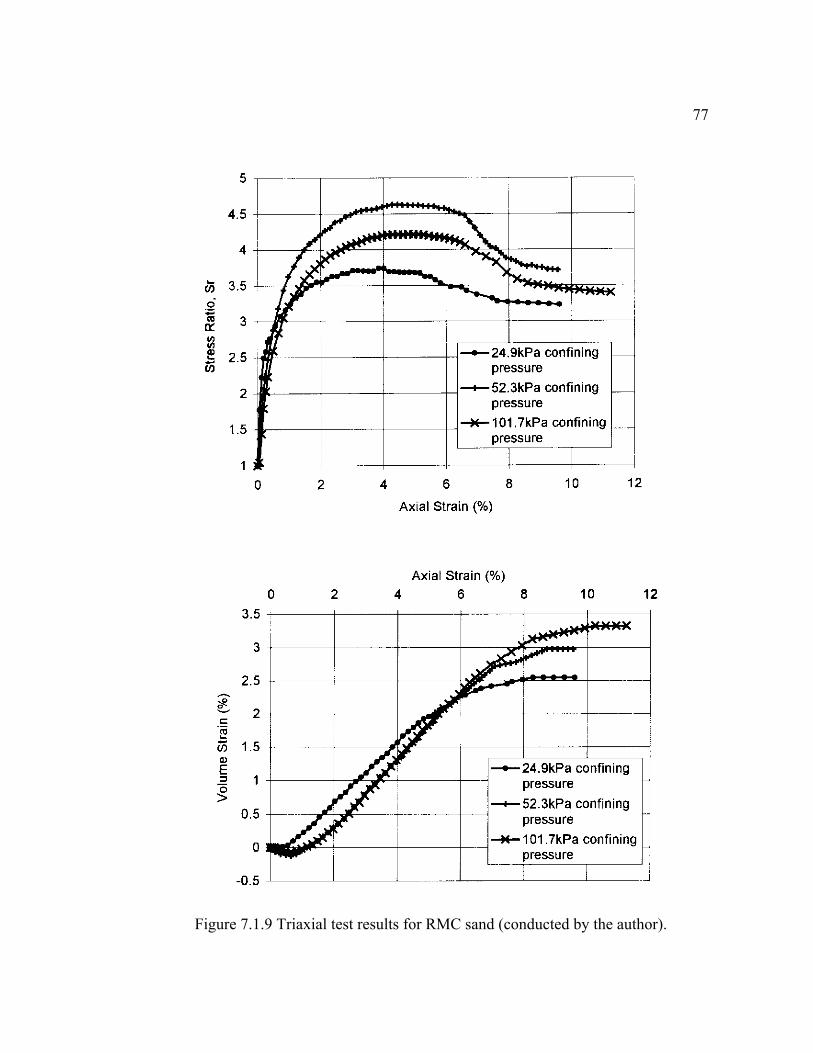
77
Figure 7.1.9 Triaxial test results for RMC sand (conducted by the author).

78
Table 7.1.5 Summary of strength properties of RMC sand.
Test Condition (confining pressures)
Initial Modulus,
(kN/m2)
1% Strain Secant Modulus, (kN/m2)
Friction Angle1,
(deg) 20 kPa 3.5 E+4 1.5 E+4 41
30 kPa 4.0 E+4 2.0 E+4 42
Plane Strain
80 kPa 4.0 E+4 3.8 E+4 43
25 kPa 1.3 E+4 0.8 E+4 37
50 kPa 2.3 E+4 1.8 E+4 38
Triaxial
100 kPa 3.6 E+4 3.2 E+4 39 1 Calculated using equation φ = Sin-1[(Sr-1)/(Sr+1)], where Sr = (σ1/σ3) at peak.

797.1.3 Summary of Plane Strain Soil Properties
In the following sections, plane strain soil properties of three tested granular soils are
summarized. Because testing soils under plane strain conditions is not very common,
these test data were also used to examine some empirical relationships that have been
proposed to convert conventional triaxial test results to plane strain soil properties.
The plane strain soil friction angles of rounded uniform sand such as Ottawa sand
were found to be only slightly higher than triaxial friction angles at low confining
pressures. However, for angular material such as the Rainier and RMC sands, the
tendency that soils posses a higher friction angle under plane strain conditions than
under triaxial conditions is clear. For granular material, Lade and Lee (1976) proposed
an empirical equation (Equation 7.1.1) to convert the triaxial friction angle to a plane
strain friction angle. Equation 7.1.1 was able to predict the low confining pressure
plane strain soil friction angles within a reasonable range (Table 7.1.6). It tends to
over-predict the plane strain friction angles of Ottawa sand (rounded sand), and under-
predict the plane strain friction angles of Rainier Sand and RMC sand (angular sands)
at low confining pressures.
φ φ φ
φ φ φps tx
otx
o
ps tx txo
= − >
= ≤
15 17 34
34
. ( )
( ) (7.1.1)
where φps = plane strain soil friction angle, and
φtx = soil friction angle obtained from triaxial tests.
80The tendency that plane strain soil moduli are higher than triaxial soil moduli is
clearly supported by test data presented in Tables 7.1.3 to 7.1.5. For uniform rounded
material like Ottawa sand, its plane strain initial moduli were about 70% higher than
triaxial initial moduli. However, its plane strain 1% strain secant moduli were only
slightly higher than triaxial 1% strain secant moduli (Table 7.1.3). For angular
material in dense state, results of Rainier sand tests indicated that the plane strain
initial moduli can be as high as seven times the triaxial initial moduli. Even for the 1%
strain secant moduli, the plane strain moduli were still about twice as high as the
triaxial moduli (Table 7.1.4). For angular material in loose state, results of RMC sand
tests indicated that both initial and 1% strain secant moduli obtained from plane strain
tests were about twice as high as those obtained from triaxial tests at low confining
pressure range (Table 7.1.5). However, when high confining pressures were applied to
RMC sand at a low relative density, a similar tendency could not be found.
To further characterize the plane strain soil moduli, the hyperbolic soil modulus
model developed by Duncan and his co-workers (Duncan and Chang, 1970; Duncan et
al., 1980) was used in the following section to analyze RMC sand plane strain test data.
7.1.4 Effects of Confining Pressure – Corrected Hyperbolic Soil Modulus Models for
Plane Strain Conditions
For geological materials such as soil, stiffness (modulus) is found to increase with
increasing confining pressure. Duncan and Chang (1970) developed a hyperbolic soil
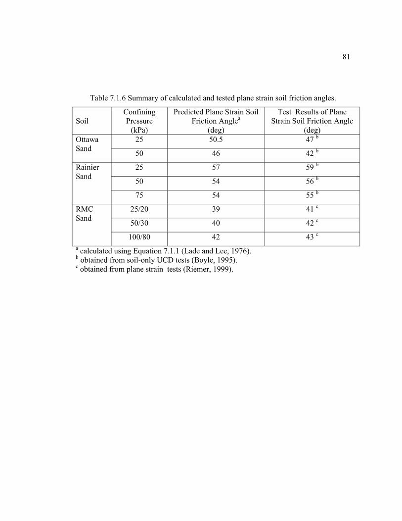
81
Table 7.1.6 Summary of calculated and tested plane strain soil friction angles.
Soil
Confining Pressure
(kPa)
Predicted Plane Strain Soil Friction Anglea
(deg)
Test Results of Plane Strain Soil Friction Angle
(deg) 25 50.5 47 b Ottawa
Sand 50 46 42 b
25 57 59 b
50 54 56 b
Rainier Sand
75 54 55 b
25/20 39 41 c
50/30 40 42 c
RMC Sand
100/80 42 43 c a calculated using Equation 7.1.1 (Lade and Lee, 1976). b obtained from soil-only UCD tests (Boyle, 1995). c obtained from plane strain tests (Riemer, 1999).

82modulus model for characterizing nonlinear (hyperbolic) stress-strain behavior of soil
under different confining stresses. Equation 7.1.3 is the mathematical expression of
hyperbolic model of soil tangent modulus (Duncan et al. 1980). It has been
extensively used in numerical analyses to simulate the confining stress dependent
modulus change of soil. In this research, Eq. 7.1.3 was also programmed by the author
into FLAC code to improve the modeling results.
( )( ) n
atm
3atm
2
3
31ft P
PKsin2cosc2
sin1R1E
σ⋅⋅⋅
φ⋅σ+φ⋅
σ−σφ−−= (Eq. 7.1.3)
where Et = Young's modulus,
Rf, K, n = model parameters,
Patm = atmospheric pressure,
φ = soil friction angle,
c = soil cohesion,
σ1 = effective vertical (overburden) pressure, and
σ3 = effective confining pressure
In Equation 7.1.3, model parameters Rf and n are the failure ratio and modulus
exponent that define the hyperbolic relation between the soil modulus and confining
pressure. K is the modulus number that determines the scale of the soil modulus. The
values of Rf, K and n can be determined using stress-strain data obtained from strength
tests (Duncan et al., 1980), mostly obtained from triaxial test data. For soil under plane
strain loading conditions, the stress-strain relationship is different from that of soil

83under triaxial conditions. Therefore, different model parameters should be used to
describe the pressure dependent soil modulus under plane strain loading conditions.
Figure 7.1.10 shows the curve fitting result of the triaxial test data of RMC sand
(where Rf = 0.73, K = 850, and n = 0.5). Plane strain test data of RMC sand tested at
low confining pressures showed a stress-strain curve similar to triaxial test data. To
curve fit the plane strain test data, the model parameter K had to be increased to 2000
for best curve fitting result while the other parameters, Rf and n, remained constant
(Figure 7.1.11).
Because most of the case histories analyzed in this research (Chapter 9) had only
triaxial test data available, the following adjustments to the hyperbolic soil modulus
model were used to convert triaxial soil moduli to plane strain soil moduli:
1. Increase the modulus number K obtained from triaxial test data by 100% to
account for the large values of the plane strain soil moduli, and
2. Use the same failure ratio (Rf) and modulus exponent (n) obtained from triaxial
test. This procedure is based on the observation that plane strain stress-strain
curves of soils analyzed in this research had similar shapes as the triaxial
stress-strain curves at strain levels less than the peak strain.
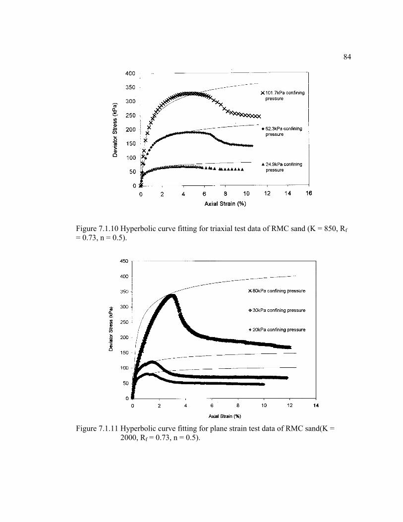
84
Figure 7.1.10 Hyperbolic curve fitting for triaxial test data of RMC sand (K = 850, Rf = 0.73, n = 0.5).
Figure 7.1.11 Hyperbolic curve fitting for plane strain test data of RMC sand(K =
2000, Rf = 0.73, n = 0.5).
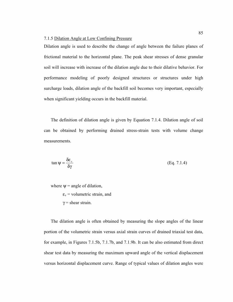
857.1.5 Dilation Angle at Low Confining Pressure
Dilation angle is used to describe the change of angle between the failure planes of
frictional material to the horizontal plane. The peak shear stresses of dense granular
soil will increase with increase of the dilation angle due to their dilative behavior. For
performance modeling of poorly designed structures or structures under high
surcharge loads, dilation angle of the backfill soil becomes very important, especially
when significant yielding occurs in the backfill material.
The definition of dilation angle is given by Equation 7.1.4. Dilation angle of soil
can be obtained by performing drained stress-strain tests with volume change
measurements.
δγδε
=ψ vtan (Eq. 7.1.4)
where ψ = angle of dilation,
εv = volumetric strain, and
γ = shear strain.
The dilation angle is often obtained by measuring the slope angles of the linear
portion of the volumetric strain versus axial strain curves of drained triaxial test data,
for example, in Figures 7.1.5b, 7.1.7b, and 7.1.9b. It can be also estimated from direct
shear test data by measuring the maximum upward angle of the vertical displacement
versus horizontal displacement curve. Range of typical values of dilation angles were

86reported as 10 to 20 deg for granular soil tested at confining pressures higher than 100
kPa (Bolton, 1986). However, dilation angles of granular soil at confining pressures
less than 100kPa have apparently not yet been investigated. Table 7.1.7 lists the soil
dilation angles of Ottawa sand, Rainier sand and RMC sand at low confining pressures.
These values were determined by reducing results shown in Figures 7.1.5b, 7.1.7b and
7.1.9b. Values of soil dilation angles shown in Table 7.1.7 indicated that granular soil
at low confining pressures possesses higher dilation angles than those under high
confining pressures. For material prepared in a dense state, the low confining pressure
dilation angles were as high as 40 degrees. Even for material prepared in loose state,
the low confining pressure dilation angles were 26 deg. This observation is very
important to working stress analyses of GRS retaining structure analyses because the
major portion of wall deflections were observed during the construction stage when
confining pressures of backfill soil are very low. Values of soil dilation angles shown
in Table 7.1.7 were used as the inputs of the developed numerical models of GRS
walls developed in this research.
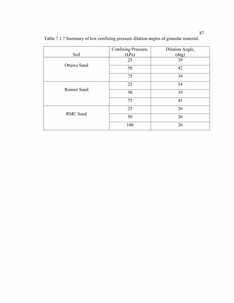
87Table 7.1.7 Summary of low confining pressure dilation angles of granular material.
Soil
Confining Pressure, (kPa)
Dilation Angle, (deg)
25 39
50 42
Ottawa Sand
75 39
25 34
50 39
Rainier Sand
75 45
25 26
50 26
RMC Sand
100 26

887.2 Geosynthetic Reinforcement Properties
7.2.1 Material Types and Structures
Most geosynthetic reinforcements are manufactured using polypropylene, polyester,
and polyethylene polymers. Table 7.2.1 lists the index properties of these polymers.
Due to these basic polymer differences, geosynthetic reinforcements that are
manufactured using different polymers have different mechanical properties,
especially, when different loading conditions or environmental conditions such as
strain rate and temperature exist.
Fabric structure is another important factor that affects the mechanical properties
of various geosynthetic reinforcements. Common geosynthetic structures include
nonwoven and woven geotextiles and geogrid structures.
Most of the geotextiles are manufactured using polypropylene and polyester
polymers (Table 7.2.1). The woven fabrics are made on conventional textile-weaving
machinery into a wide variety of fabric weaves. In contrast, nonwoven fabrics are
usually manufactured by heat-bonding or needle-punching the fibers (continuous
filaments or long staple fibers) into the geotextile sheets. Details on manufacturing
processes and basic properties of geotextiles can be found in Koerner (1998).
Generally speaking, woven geotextiles have higher strengths than nonwoven
geotextiles because of their structures. For woven geotextiles, multifilament
geotextiles have higher tensile strengths than monofilament geotextiles, and
monofilament geotextiles have higher tensile strengths than the slit film geotextiles.
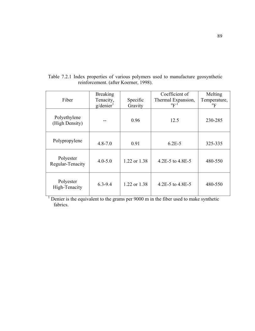
89
Table 7.2.1 Index properties of various polymers used to manufacture geosynthetic
reinforcement. (after Koerner, 1998).
Fiber
Breaking Tenacity, g/denier1
Specific Gravity
Coefficient of Thermal Expansion,
oF-1
Melting Temperature,
oF
Polyethylene (High Density)
--
0.96
12.5
230-285
Polypropylene
4.8-7.0
0.91
6.2E-5
325-335
Polyester
Regular-Tenacity
4.0-5.0
1.22 or 1.38
4.2E-5 to 4.8E-5
480-550
Polyester
High-Tenacity
6.3-9.4
1.22 or 1.38
4.2E-5 to 4.8E-5
480-550
1 Denier is the equivalent to the grams per 9000 m in the fiber used to make synthetic fabrics.
90For nonwoven geotextiles, heat-bonded geotextiles usually have a higher strength than
needle punched geotextiles for the same mass per unit area.
The polymer materials used in the manufacture of oriented geogrids are high-
density polyethylene, polypropylene or polyester. There are two types of geogrids.
Stiff geogrids are made by punching patterned holes into heavy gauge sheets of
polyethylene or polypropylene and then drawing the sheets at controlled temperature
and strain rate. Flexible geogrids are made by weaving high-tenacity polyester yarns
into an open structure with the junctions being knitted together or physically
interwined into transverse and longitudinal ribs. Additional information about geogrid
types, manufacture, and basic properties can be found in Koerner (1998).
When geosynthetic reinforcement is buried in soil, different types tend to have
different interactions with the surrounding soil. Therefore, in-soil properties of
geosynthetic reinforcement are often different from their in-isolation properties.
Similarly, reinforcement-soil interfaces also are different between different
geosynthetic reinforcement.
In the following sections, two important factors that influence the in-soil
performance of geosynthetic reinforcement, soil confinement and strain rate, are
described. Their effects on the properties of geosynthetic reinforcement inside GRS
91structures, as well as appropriate property adjustments to account for these factors, are
discussed.
7.2.2 Effect of Soil Confinement
As noted above, when buried in soil, geosynthetic reinforcement may have a very
different behavior than it has in isolation. The interactions between the geosynthetics
and soil also affect the properties of the geosynthetic reinforcement.
When buried in soil, the loose filament structure of nonwoven geosynthetics tends
to be compressed by the soil and also allowes soil particles to enter the spaces in
between the filaments. The apparent stiffness of this filament-soil composite then
becomes the in-soil stiffness of the nonwoven geotextile. There is strong evidence that
nonwoven geotextiles do in fact have greater moduli and strengths when they are
confined in soil (McGown et al., 1982; El-Fermaoui and Nowatzki, 1982; Leshchinsky
and Field, 1987; Wu and Arabian, 1990; Ling et al., 1992). Results of the UCD tests
also indicated that the tensile moduli of nonwoven geosynthetics increased when the
geosynthetics were confined in soil (Boyle, 1995). Thus the increase of stiffness of
nonwoven geotextiles is controlled by the structure of the geotextile and the confining
pressure.
At present, because of difficulty of testing geosynthetic reinforcement in soil, the
magnitude of stiffness increase of nonwoven geosynthetic reinforcement has not yet

92been well characterized. However, the soil confining effect has to be considered when
selecting the tensile modulus for the nonwoven geosynthetic reinforcement.
Soil confinement seems to have minimal effect on the stress-strain behavior of
woven geosynthetic or geogrid reinforcements. Boyle (1995) found that the tensile
moduli of woven geotextiles were not significantly influenced by confinement in the
UCD device. The in-isolation tensile modulus of the woven geosynthetic
reinforcement can be used as the in-soil tensile modulus.
No specific in-soil properties of geogrids have been measured. Koerner (1998)
commented that the tensile moduli of geogrids are probably not affected very much by
confinement based on the in-soil tests of nonwoven and woven geotextiles.
Interaction between soil and geosynthetic reinforcement is another important issue
beside the in-soil confinement that needs to be characterized for performing working
stress analyses of GRS walls. Holtz (1977) and Jewell (1984) both concluded that the
interaction between soil and geosynthetic reinforcement is controlled by the particle
size of the surrounding soil and the apertures of the geotextiles or geogrids. For cases
that the soil particle is small enough to enter the fabric apertures, the interlocks
between soil and geosynthetics allow pullout resistance close to the full shearing
resistance of the soil to develop. Results of UCD tests (Boyle, 1995) indicated that the
shear surfaces did occur in the soil next to the reinforcement when loading GRS
93specimens in the UCD. For GRS wall case histories collected in this research, all
backfill soils had a D50 less than 1mm (Figure 7.1.3), i.e. most particles of these
backfill soils has sizes smaller than the apertures of the reinforcements used in these
case histories. Complete interlock between soil particles and geosynthetic
reinforcement is assumed. Properties of backfill (internal friction angle and elastic
modulus) were used as the interface properties of the geosynthetic reinforcements in
this research.
7.2.3 Effect of Strain Rate
Mechanical properties of geosynthetic reinforcement were also found to be affected by
the strain rate. Boyle et al. (1996) reported that the moduli of woven geotextiles
decreased when they were tested at a low strain rate. Strength properties of
geosynthetic reinforcement are often obtained by performing ASTM D 4595 wide
width tensile tests. However, the actual rate of loading of the reinforcement in the field
during wall construction may be five or six orders of magnitude slower than the
standard ASTM D 4595 wide width testing rate of 10%/min. In order to model the
working stress conditions inside GRS retaining structures, the moduli of geosynthetic
reinforcement had to be adjusted for the low strain rate conditions that really existed
during wall construction. Wide width tensile and UCD tests conducted at low strain
rates to simulate actual loading rates in full scale structures have indicated that
reductions in tensile moduli are needed to account for the slow loading of the
reinforcement (Boyle 1995; Boyle at al., 1996; Holtz and Lee, 1998). However,

94magnitudes of these modulus reductions are found to be dependent upon following
factors:
1. The actual strain rate (rate of loading),
2. The properties of the polymer fibers used in the reinforcement,
3. Structure of the reinforcement,
4. Unit weight of the reinforcement,
5. In-isolation stiffness of the reinforcement, and
6. Temperature.
For nonwoven geotextiles, because of the random filaments and very different
index properties between different products, modulus reductions have not yet been
clearly characterized. For woven reinforcement made of polypropylene, a 50%
reduction of the in-isolation modulus obtained from the wide width tensile test (ASTM
D 4595) is recommended as the low strain rate adjustment (Holtz and Lee, 1998). For
woven reinforcement made of polyester, a 20% reduction of modulus obtained from
the wide width tensile test (ASTM D 4595) is recommended (Holtz and Lee, 1998).
For HDPE geogrids, 50% modulus reduction on wide width tensile modulus is
recommended (Lee, Holtz, and Allen, 1999).

957.3 Conclusions
In this chapter, soil and geosynthetic properties inside the GRS walls were discussed.
Adjustments that convert soil and geosynthetic properties obtained from conventional
tests into those inside the GRS walls were also presented. These adjustments can be
summarized as:
1. Convert triaxial or direct shear soil friction angles to plane strain soil friction
angles using Equations 7.1.1 and 7.1.2;
2. Calculate plane strain soil modulus using the modified hyperbolic soil modulus
model;
3. Investigate the appropriate dilation angles of the backfill material;
4. Investigate the effect of soil confinement on reinforcement tensile modulus;
and
5. Apply appropriate modulus reduction on reinforcement tensile modulus to
account for the low strain rate that occurs during wall construction.
As described in Section 3.4, inaccurate input of material properties was one of the
major reasons why no working stress analyses have been successfully performed on
GRS walls in the past. Adjustments of material properties summarized above were
utilized in this research to model the performance of GRS walls. Successful modeling
results were obtained. Detailed descriptions of how these adjustments are implemented
in the modeling techniques used for GRS retaining structure performance prediction
are presented in Chapter 8.

96Chapter 8
Developing Numerical Models of GRS Retaining Structures Using the
Computer Program FLAC
In this research, numerical techniques were used to perform the internal stability
analyses of GRS retaining structures. A finite difference method based computer
program, FLAC (Fast Lagrangian Analysis of Continua), was used to perform
working stress analyses for GRS retaining structures. FLAC was selected for this
research because of its excellent capability of modeling geotechnical engineering
related stability problems and its extended programming ability. Although numerical
analyses using FDM usually have longer iteration times than FEM, with the
development of high-speed computers, this is not a major shortcoming. Both discrete
and composite models were developed using the FLAC program. Moreover, a
practical (simplified) calculation method of working stress analyses for GRS retaining
structures was also developed after a detailed parametric study was performed on the
design factors of GRS retaining structures using FLAC. Details of the development of
numerical models using FLAC program are described in this Chapter.
8.1 General Description of FLAC
The FLAC program is a two-dimensional explicit finite difference program developed
for mining and civil engineering projects. Large strain behavior such as plastic
collapse and flow of structures can be modeled using the explicit, Lagrangian,
calculation scheme and the mixed-discretization zoning technique of FLAC (Itasca,

971995). The FLAC program was originally developed for geotechnical and mining
engineers. In FLAC, materials are represented by elements whose behavior follows a
prescribed linear or non-linear stress/strain law when external forces or boundary
restraints are applied. Users can form these material elements into a grid to represent
the shape of the modeled object. FLAC also provides a FISH programming code to
allow users to define their own constitutive material models. Besides the material
models, FLAC also provides some built-in structural elements that can be used as
reinforcement or structural supports. These structural elements can be embedded into
the grid mesh without any geometric restrictions, and they can be fully incorporated
with the surrounding material elements according to their specified built-in interface
properties. Another special feature that FLAC provides is interface elements. Interface
elements allow FLAC to simulate distinct planes along which slip and/or separation
can occur.
Figure 8.1.1 shows a typical section of a GRS retaining structure that was modeled
using FLAC. As shown in the figure, elements of elastic material, Mohr-Coulomb
material, cable, and interfaces can be used to develop FLAC models of GRS retaining
structures. In this research, the transversely isotropic elastic material model within
FLAC was also used to develop the composite material approach for GRS retaining
structures. In the following sections, specific input properties as well as modeling
guidelines for different material models are described. Detailed formulation of these
material and structural elements can be found in the FLAC manuals (Itasca, 1995).
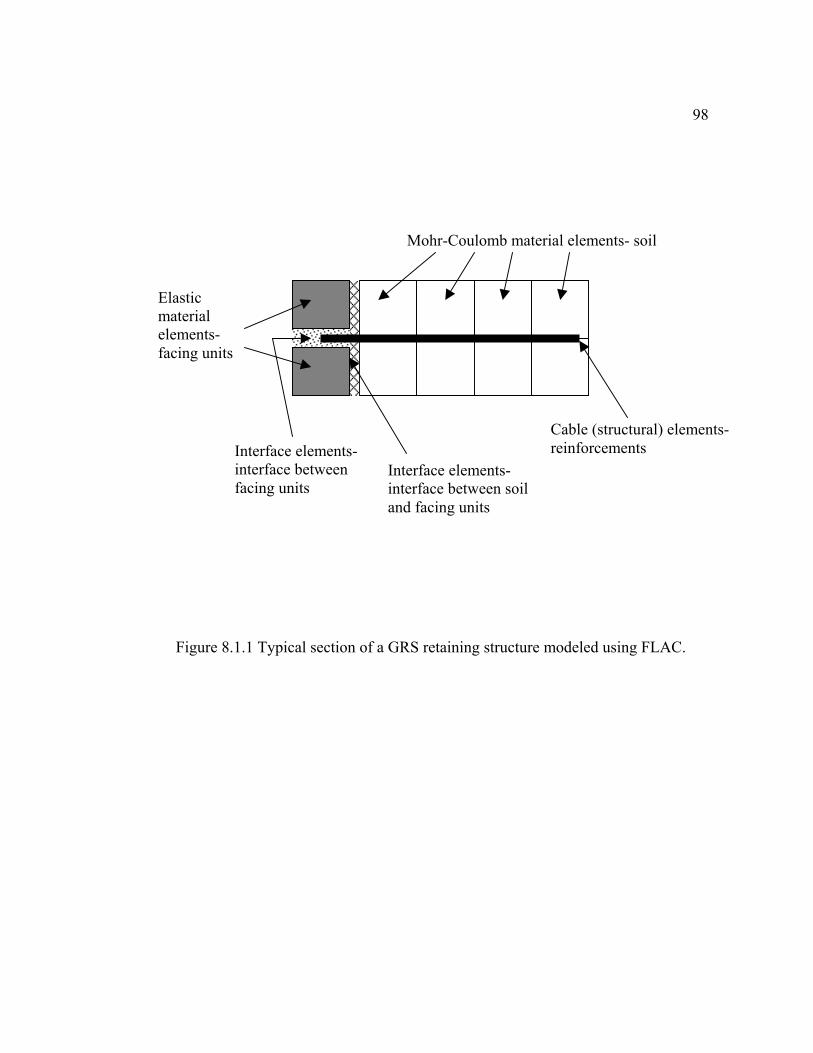
98
Figure 8.1.1 Typical section of a GRS retaining structure modeled using FLAC.
Interface elements- interface between soil and facing units
Mohr-Coulomb material elements- soil
Cable (structural) elements-reinforcements Interface elements-
interface between facing units
Elastic material elements- facing units

998.2 Built-in Material Models
In the following sections, the built-in constitutive material models of FLAC program
that were used to assemble the numerical models of GRS retaining structures are
summarized according to their basic stress-strain behavior, applications in model
development, and input properties.
8.2.1 Elastic Material Model
The elastic material model is the model with a linear stress-strain relationship. Elastic
material elements were usually used to represent the facing as well as the reaction wall
and concrete foundation plate of large scale test walls. Input properties of the elastic
material elements were the material density, and the bulk and shear moduli of the
material.
8.2.2 Transversely Isotropic Elastic Material Model
Besides the elastic and Mohr-Coulomb material models, the transversely isotropic
elastic material model was also used to develop composite GRS retaining structure
models. The transversely isotropic elastic material elements allow the user to specify
the stress-strain properties (elastic modulus and Poisson’s ratio) in two principal
directions rather than assign isotropic stress-strain properties. In this research,
transversely isotropic elastic material elements were used to describe the transversely
isotropic behavior of the GRS composite material.

1008.2.3 Mohr-Coulomb Material Model
The Mohr-Coulomb material model is actually an elasto-plastic material model. The
Mohr-Coulomb elements are mainly used for the backfill soil of the GRS retaining
structures. By adding three more input properties, the friction angle, cohesion and
dilation angle, onto the elastic material, the shear failure (plastic yielding) of material
can be simulated.
The soil friction angle and cohesion (if any) can be obtained from laboratory soil
strength tests such as direct shear tests, triaxial tests, or other appropriate soil strength
tests. However, each of these laboratory tests simulates different loading conditions
and therefore provides different values of friction angle and cohesion even when the
same material is tested. Test results have to be carefully converted to input properties
that can accurately represent the real loading conditions inside GRS retaining
structures.
Another important input property of Mohr-Coulomb material elements is the
dilation angle. The physical meaning of the dilation angle was described in Chapter 7.
This input property is very important when larger strain situations are modeled such as
structures with large surcharges, structures designed with a low factor of safety, and
structures under dynamic loading. The value of the dilation angle can be determined
from triaxial or direct shear test data with volumetric measurements. Table 7.1.6 listed
values of dilation angles of backfill material analyzed in this research.
101Advantages of using the Mohr-Coulomb material model for the backfill includ:
1. The model provids a yielding criteria (failure envelope) similar to the backfill
material (soil), and
2. The input properties of Mohr-Coulomb material model can be obtained from
regular soil strength tests such as direct shear test and triaxial test.
8.2.4 Pressure Dependent Soil Modulus Model
Because face deflections and other movements have been observed during the
construction of real and test GRS walls, it is very important to simulate the wall
construction in order to have an accurate prediction of wall performance. During GRS
wall construction, the backfill material is placed and compacted layer by layer. The
confining pressure of the backfill material is of course very small when each lift is first
placed. As the height of the wall increases, the confining pressures in the finished lifts
increase. At the end of construction, the lower part of the wall has a higher confining
pressure, and the upper part of the wall has lower confining pressure. This confining
pressure change of the backfill has a very important effect on the performance of the
GRS walls, because moduli of soil are actually pressure dependent, especially for
granular soils. Moduli of granular soil increase as the confining pressures increase. In
order to include the confining pressure effects on soil modulus during construction,
the modified hyperbolic soil modulus model described in Section 7.1.4 was also
introduced into the FLAC Mohr-Coulomb material model. Equation 7.1.3 (Duncan et
102al., 1980) was programmed as a FISH subroutine that updates the soil moduli
according to the stress conditions of the soil elements. Details of the development of
this subroutine are described in Section 8.5.4.
8.3 Interface Elements
The FLAC program also provided interface elements to enable the simulation of the
contacts between different materials. As shown in Figure 8.1.1, two different types of
interfaces were used in a GRS retaining structure model: the interfaces between facing
units and the interfaces between soil and structural objects like the wall face. The
interface elements were also used to simulate the contacts between the backfill and
reaction wall or concrete foundation of the in-laboratory large-scale test walls. Figure
8.3.1 shows the mechanical representation of the interface (Itasca, 1995). In FLAC,
the interface element is characterized by Coulomb sliding and/or tensile separation
elements. Input properties for the interface elements include friction, cohesion, normal
and shear stiffness, and tensile strength. Determination of these input properties for
GRS retaining structures is described in Section 8.5.7.
8.4 Cable Element—Structural Elements for Modeling Reinforcements
There are four different forms of structural elements in FLAC: beam, cable, pile, and
support elements. Both beam and cable elements can be used to model reinforcements.
Cable elements were chosen in this research to represent the geosynthetic
reinforcement because of their ability to provide sufficient information on the
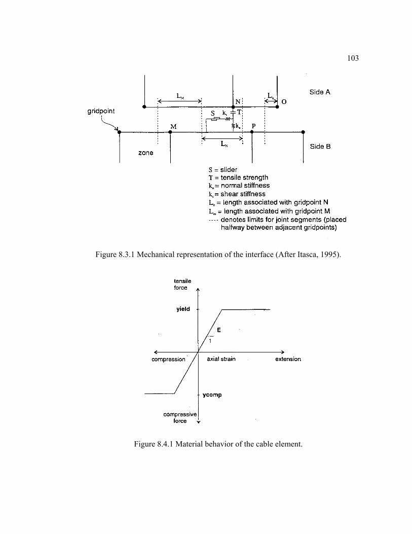
103
Figure 8.3.1 Mechanical representation of the interface (After Itasca, 1995).
Figure 8.4.1 Material behavior of the cable element.
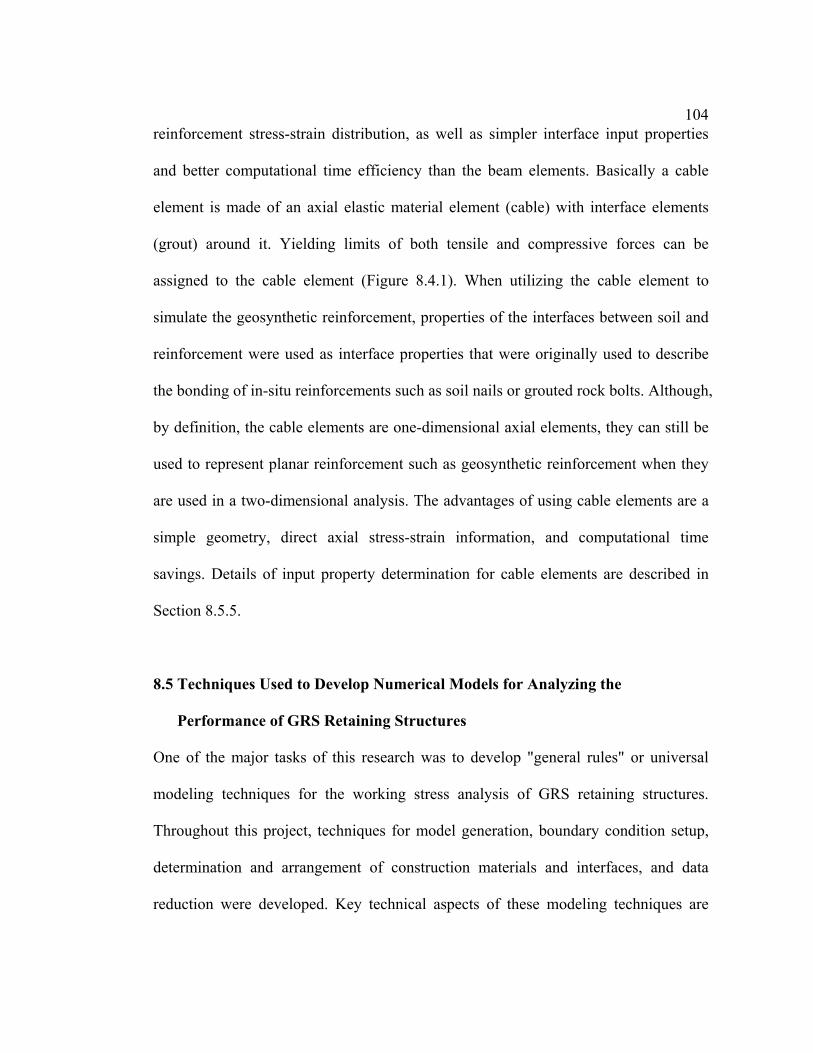
104reinforcement stress-strain distribution, as well as simpler interface input properties
and better computational time efficiency than the beam elements. Basically a cable
element is made of an axial elastic material element (cable) with interface elements
(grout) around it. Yielding limits of both tensile and compressive forces can be
assigned to the cable element (Figure 8.4.1). When utilizing the cable element to
simulate the geosynthetic reinforcement, properties of the interfaces between soil and
reinforcement were used as interface properties that were originally used to describe
the bonding of in-situ reinforcements such as soil nails or grouted rock bolts. Although,
by definition, the cable elements are one-dimensional axial elements, they can still be
used to represent planar reinforcement such as geosynthetic reinforcement when they
are used in a two-dimensional analysis. The advantages of using cable elements are a
simple geometry, direct axial stress-strain information, and computational time
savings. Details of input property determination for cable elements are described in
Section 8.5.5.
8.5 Techniques Used to Develop Numerical Models for Analyzing the
Performance of GRS Retaining Structures
One of the major tasks of this research was to develop "general rules" or universal
modeling techniques for the working stress analysis of GRS retaining structures.
Throughout this project, techniques for model generation, boundary condition setup,
determination and arrangement of construction materials and interfaces, and data
reduction were developed. Key technical aspects of these modeling techniques are

105summarized in this section. These comments were described in terms familiar to a
FLAC program user; therefore, terminology and programming techniques of FLAC
are used. Detailed information on the terminology and basic programming commands
of FLAC are described in the FLAC manuals (Itasca, 1995).
8.5.1 Model Generation
1. Four kinds of material elements described in the previous sections, elastic
material elements, Mohr-Coulomb material elements, structure (cable) elements,
and interface elements, were used to create models of GRS retaining structures.
1.1 Elastic material elements were used to represent the material with higher
strength and a linear stress-strain behavior under working stresses. They were
used to represent different facing materials such as precast concrete panels,
modular blocks, or rock-filled gabion baskets. They were also used to
represent the concrete foundation and the reaction wall of the large-scale test
walls built in the laboratory (Chapter 10).
1.2 Mohr-Coulomb material elements were used to represent the soil, including
the backfill and foundations of GRS retaining structures.
1.3 Cable elements were used to represent the geosynthetic reinforcement.
1.4 Interface elements were used to describe the interaction between different
materials or the discontinuities between the same materials such as interfaces
between backfill soil and structural facing, and interfaces between structural
facing units.
106
2. When setting up the grids for FLAC models of GRS retaining structures, at least
three rows of soil elements should be inserted in between reinforcement layers.
This technique allows users to observe the interaction between the reinforced
composite layer (soil elements with reinforcement elements attaching to their
nodes) and the soil-only layer.
3. An aspect ratio of 0.5 to 2 is recommended for elements within the reinforced
zone (the aspect ratio is the ratio of the height to the length of the element). In
FLAC, the aspect ratio is limited to a range of 0.2 to 5. Having an aspect ratio
close to a value of one helps not only to reduce the iteration time, but it also
ensures stress or strain equilibrium inside the elements when the stress ratio limit
is set for the equilibrium criteria. The disadvantage of using aspect ratios close to
one is that the number of total elements increases considerably when the size of
the modeling object is large or when the reinforcement layout of the modeling
project is complicated.
4. The program command that allows large strain calculations has to be used in order
to allow for post-yielding behavior to occur in material elements, especially in the
backfill material. This technique helps the designer to identify the high stress-
strain zones, including a failure surface, if any, inside the modeling structure
107especially when the structure is poorly designed. FLAC program command to
allow large strains to occur is “set large” 1.
8.5.2 Boundary Conditions
In numerical analyses, the boundary conditions have to be carefully set up to avoid
any artificial reaction forces or deformations to occur. The following
recommendations are for static analyses of GRS retaining structures only. Boundary
condition criteria must be carefully investigated if dynamic analyses are performed.
1. The unreinforced backfill of the GRS retaining structure models should be
extended a distance equal to at least the length of “reinforced zone” to eliminate
boundary effects. For cases in which the reinforced backfill has an irregular shape
or intersects bedrock, the actual boundary conditions should be modeled.
2. To eliminate boundary effects, the foundation part of the GRS retaining structure
models should be extended to a depth at least equal to the height of the GRS wall
or to bedrock. However, when the settlement of the GRS retaining structure is a
major issue, the foundation soil should be extended to a depth that would cover all
the compressible soil layers that might contribute to the total settlement of the
structure.
1 Bold words are the commands or symbols used in FLAC
1083. For the portion in front of the wall face, as with the unreinforced backfill, an
irregular shape or shorter length boundary has to be modeled. Otherwise, the
horizontal boundary in front of the wall face should be extended at least equal to
the length of reinforcement to eliminate boundary effects.
4. When developing numerical models of laboratory-scale test walls, the boundary
conditions of the test facilities such as the reaction wall, the concrete foundation,
and any toe restraints have to be carefully set up. (In Chapter 10, the difference
between laboratory test walls and real walls is discussed and summarized, based
on results of numerical models with different boundary conditions.)
8.5.3 Equilibrium Criteria
With FLAC. to ensure that the results of the numerical analysis have converged and
that the unbalanced forces within individual material elements have been minimized, it
is necessary to set up equilibrium criteria.
Within FLAC, users can set limits on the unbalanced force and/or stress ratio of
the material elements as the equilibrium criteria. Each grid point in the FLAC model is
surrounded by up to four material elements. The algebraic sum of forces contributed
by these surrounding elements at any specific grid point should converge to zero when
the model reaches equilibrium. This algebraic sum of forces acting on the grid point is
defined as the unbalanced force. In FLAC analyses, users can define equilibrium
109criteria by setting limits on the unbalance forces. However, these forces are calculated
by multiplying the stresses within the elements by the element lengths perpendicular
to the forces. Small values of unbalanced forces might not indicate a converging
equilibrium result when models have very small grid sizes.
The stress ratio is defined as the ratio of maximum unbalanced force to the
representative internal force. The grid size is no longer a factor that affects the
equilibrium convergence when stress ratio is used to set up the equilibrium criteria. In
this research, a stress ratio less than 0.01 was used as the equilibrium criteria for
intermediate stages (during wall construction) and stress ratio less than 0.001 was used
as the equilibrium criteria for final stages (after construction, and after surcharges).
8.5.4 Hyperbolic Soil Modulus Model
As described in Section 8.2.3, the hyperbolic soil modulus model was used to simulate
the change of soil modulus due to confining pressure change during wall construction.
In this research, a FISH subroutine was developed to update the moduli of Mohr-
Coulomb material (soil) elements automatically according to the change of the
confining pressure. This subroutine was edited based on the hyperbolic soil modulus
model (Equation 7.1.3). Example 8.5.1 shows the FLAC code of this subroutine. In
Example 8.5.1, the area that needs this modulus adjustment is defined by parameters
vi, vf, hi, and hf. Bulk_mod(i,j) and Shear_mod(i,j) are bulk and shear moduli of the
element defined by horizontal grid number i and vertical grid number j. nu is the

110
Example 8.5.1 FISH subroutine for updating soil modulus according the confining pressure – Hyperbolic soil modulus model.
******************************************************************
def janbu2 loop j (vi,vf) loop i (hi,hf) temp1=-0.5*(sxx(i,j)+syy(i,j)) temp2=sqrt(sxy(i,j)^2+0.25*(sxx(i,j)-syy(i,j))^2) sigma3=min(temp1-temp2, -szz(i,j)) if sigma3<0 then sigma3=0.0 end_if sl=max(temp1+temp2, -szz(i,j)) sl=0.5*(sl-sigma3)*(1-sin(fri*degrad)) sl=sl/(coh*cos(fri*degrad)+sigma3*sin(fri*degrad)) ela=(1-rf*sl)^2*k1*pat*(sigma3/pat)^nd bulk_mod(i,j)=ela/(3*(1-2*nu)) shear_mod(i,j)=ela/(2*(1.0+nu)) end_loop end_loop end
************************************************************************************ def supstep janbu command step 100 end_command end
************************************************************************************ def supsolve loop kk(1,10) supstep end_loop end
************************************************************************************ set fric=45 coh=0 nu=0.25 set k1=2000 rf=0.73 nd=0.5 set pat=101.3
******************************************************************

111Poisson’s ratio of the backfill material. As described in Section 7.1.4, the model
parameters k1, rf, and nd have to be modified for plane strain loading conditions
when using this subroutine to model structures like GRS retaining walls.
8.5.5 Determination of Reinforcement Input Properties
Input properties of cable elements can be divided into two categories: the strength
properties and geometric properties. The strength properties include:
1. Elastic modulus (e),
2. Tensile (yield) and compressive (ycomp) yield strengths, and
3. Stiffness (kbond), cohesive strength (sbond), and friction resistance (sfric) of
the interface.
The geometric properties include:
1. Cross-sectional area (a), and
2. Exposed perimeter (peri).
Input properties of the cable elements were computed by assuming the cable elements
have an out-of-plane depth of unity. This interpretation was verified when the model
was able to reproduce the shear resistance developed along the reinforcement of real
GRS walls. The FLAC models were not sensitive to the in-soil thickness of the cable
elements. To convert the planar strength properties of geosynthetics, an arbitrary yet
reasonable in-soil thickness was assumed. In this research, the in-soil thickness of

112geosynthetic reinforcements was set to an arbitrary and convenient 5 mm. However,
once the in-soil thickness has been decided, the cross sectional area, elastic modulus,
and perimeter of the cable element has to be calculated using the same in-soil
thickness. Example 8.5.2 is an example of input property determination of cable
elements (geosynthetic reinforcement).
In this research, the assumption was made that no slippage occurred between the
soil and the geosynthetic reinforcement, because almost no pullout failures were
observed in any of the analyzed case histories. Therefore, cable elements were fixed to
the nodes of the Mohr-Coulomb material elements to avoid violation of compatibility.
Experiences from previous modeling studies indicated that soil elements tend to
“penetrate” the cable element and cause inaccurate stress and strain information when
the model had large deformations and the cable elements were not fixed to the nodes
of the material elements. There is no need to input values of kbond, sbond, and sfric
(properties of the interface) when cable elements are fixed to the nodes of the material
elements because perfect bonding between cable and soil is assumed.
8.5.6 Arrangement of Reinforcement
In all the numerical models presented in this dissertation, the reinforcement (cable)
elements were attached to the nodes of the material elements. This technique was used
to avoid the violation of strain compatibility, such as when soil elements penetrate the
cable elements at large strains (Figure 8.5.1). However, this technique (attaching the
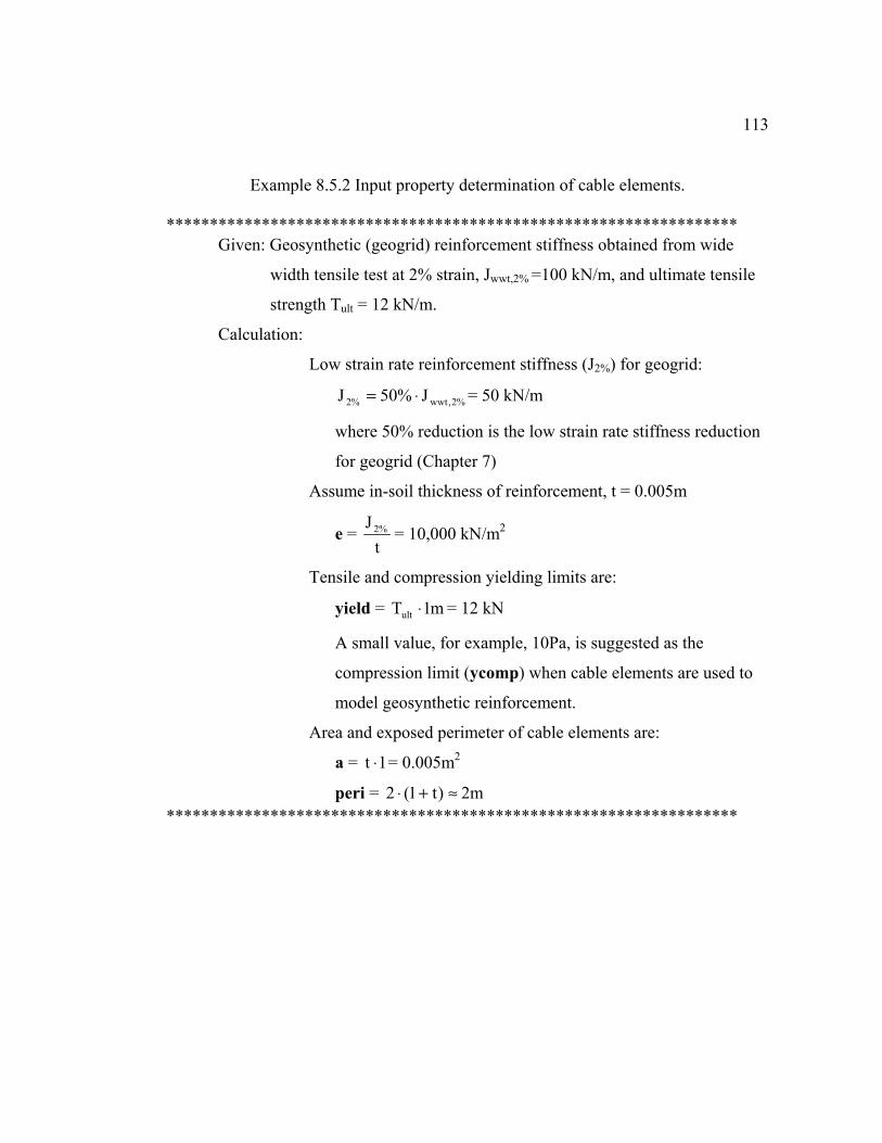
113
Example 8.5.2 Input property determination of cable elements.
****************************************************************** Given: Geosynthetic (geogrid) reinforcement stiffness obtained from wide
width tensile test at 2% strain, Jwwt,2% =100 kN/m, and ultimate tensile
strength Tult = 12 kN/m.
Calculation:
Low strain rate reinforcement stiffness (J2%) for geogrid:
%2,wwt%2 J%50J ⋅= = 50 kN/m
where 50% reduction is the low strain rate stiffness reduction
for geogrid (Chapter 7)
Assume in-soil thickness of reinforcement, t = 0.005m
e = t
J %2 = 10,000 kN/m2
Tensile and compression yielding limits are:
yield = m1Tult ⋅ = 12 kN
A small value, for example, 10Pa, is suggested as the
compression limit (ycomp) when cable elements are used to
model geosynthetic reinforcement.
Area and exposed perimeter of cable elements are:
a = 1t ⋅ = 0.005m2
peri = ≈+⋅ )t1(2 2m ******************************************************************
114cable elements to the nodes of the material) tended to over-predict the reinforcement
tension near the faces of the GRS walls because no relative movements were allowed
to occur in between the material and cable elements (Figure 8.5.1). For example,
numerical models of wrapped face walls tended to predict the peak reinforcement
tension at the wall face because soil elements near the wall face had high deflections;
however, very small reinforcement strains (tensions) were observed at the face of the
wrapped face wall in the field.
Moreover, reinforcement tensions at connections of GRS walls with structural
facing systems were also over-predicted by using this technique because the cable
elements moved with soil element without any slippage (Figure 8.5.1).
GRS wall models without fixing cable elements to the material element nodes
were also developed in this research. Properties of the backfill soil at the same levels
of the modeled reinforcement layer were used as interface properties of the
reinforcement element when the cable elements were not attached to the material
element nodes. Results of these models tended to predict smaller reinforcement
tensions than when cable elements were attached to material element nodes. For the
cases studied in this research, prediction of these (unfixed) models appears to be closer
to the instrumentation measurements. Equation 8.5.1 shows the general relations
between reinforcement tension predictions made by models with different cable
element arrangements. Values of coefficient a in Equation 8.5.1 were the average

115
(a) Before large strain occurs.
(b) After large strain occurred.
(c) Cable elements were attached to the nodes.
(d) Cable elements were not attached to the nodes.
Figure 8.5.1 Effects of attaching cable elements to the material element nodes.
Very large strain occurred only at cable elements in between the nodes
Interface between face and soil elements
Face Elements
Cable Elements
Soil Elements
Cable element floated in material elements
116ratios of reinforcement tensions predicted by models in which cable elements were not
attached to material element nodes to reinforcement tensions predicted by models in
which cable elements were attached to material element nodes. Equation 8.5.1 was
used to adjust the prediction of the model developed to predict the performance of the
GRS walls (Chapter 14).
fuf TaT ⋅= (Eq. 8.5.1)
where Tuf = reinforcement tensions were obtained from models in which cable
elements were not attached to material element nodes,
a = 0.6 at the connections of walls with structural facing systems or at the
face of the wrapped face walls,
= 0.8 reinforcement elements inside the backfill, and
Tf = reinforcement tensions were obtained from models in which cable
elements were attached to material element nodes.
Example 8.5.4 shows two FISH subroutines Hrein and Vrein that can
automatically attach cable elements to the material element nodes. Hrein is used to
assign the horizontal member of the reinforcement elements, and Vrein is used to
assign the vertical member. Users only have to input the beginning node (Rbeg) and
the ending node (Rend) of the cable elements; these two subroutines will attach the
cable elements to every material element node in between the beginning and ending
nodes. Input parameters v0 and h0 are the location nodes for vertical and horizontal

117
Example 8.5.4 FISH subroutines for attaching cable elements to material element
nodes.
****************************************************************** def Hrein h1=Rbeg Rend=Rend-1 f1=f1 v0=v0 loop i (Rbeg,Rend) h2=h1+1 command struct cable begin grid h1,v0 end grid h2,v0 seg=1 pr=f1 end_command h1=h2 end_loop end
********************************************************************** set vo= Rbeg= Rend=
********************************************************************** def Vrein v1=Rbeg Rend=Rend-1 f1=f1 h0=h0 loop j (Rbeg,Rend) v2=v1+1 command struct cable begin grid h0,v1 end grid h0,v2 seg=1 pr=f1 end_command v1=v2 end_loop end
********************************************************************** set ho= Rbeg= Rend=
******************************************************************
118members of the reinforcement elements.
8.5.7 Facing Systems
Three common facing systems were modeled in this research:
1. Fabric wrapped face--Geosynthetic reinforcement is wrapped around and
tucked back into the backfill at the wall face. No structural facing units are
used.
2. Concrete panel face--Pre-cast concrete panels are used as the structural facing
units for wall face. The concrete panels and reinforcement are connected by
pre-casting a small portion of the reinforcement in the concrete panels and then
connecting this portion to the main reinforcement when the concrete panels are
placed in position.
3. Modular block facing--Modular (pre-cast concrete) blocks are used as the
structural facing units of wall face. Geosynthetic reinforcement is inserted and
fixed in between the blocks by steel or polymer pins, clamping in block
wedges or lips, or just relying on the friction between blocks and friction of the
gravel material filled in the block units.
The fabric wrapped faced GRS retaining walls were the least complicated systems
modeled in this research, because no elastic material elements or the interface
elements were necessary to model this type of GRS wall. For GRS walls with
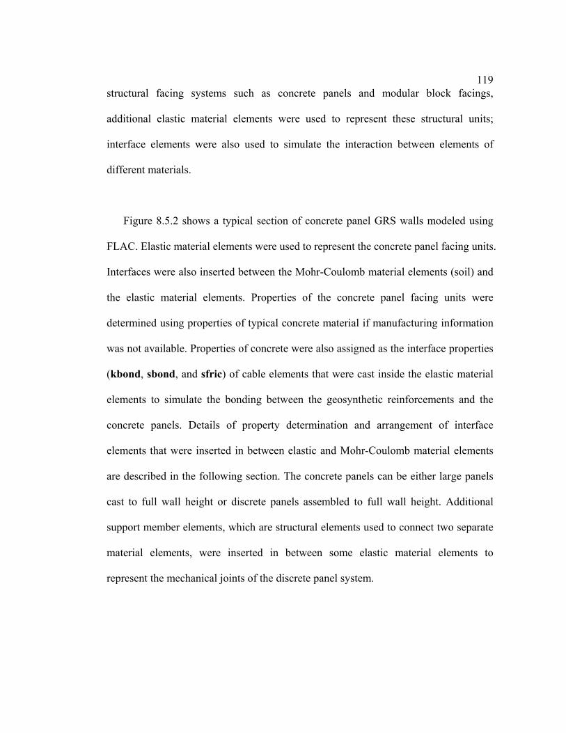
119structural facing systems such as concrete panels and modular block facings,
additional elastic material elements were used to represent these structural units;
interface elements were also used to simulate the interaction between elements of
different materials.
Figure 8.5.2 shows a typical section of concrete panel GRS walls modeled using
FLAC. Elastic material elements were used to represent the concrete panel facing units.
Interfaces were also inserted between the Mohr-Coulomb material elements (soil) and
the elastic material elements. Properties of the concrete panel facing units were
determined using properties of typical concrete material if manufacturing information
was not available. Properties of concrete were also assigned as the interface properties
(kbond, sbond, and sfric) of cable elements that were cast inside the elastic material
elements to simulate the bonding between the geosynthetic reinforcements and the
concrete panels. Details of property determination and arrangement of interface
elements that were inserted in between elastic and Mohr-Coulomb material elements
are described in the following section. The concrete panels can be either large panels
cast to full wall height or discrete panels assembled to full wall height. Additional
support member elements, which are structural elements used to connect two separate
material elements, were inserted in between some elastic material elements to
represent the mechanical joints of the discrete panel system.

120
Figure 8.5.2 Typical section of concrete panel GRS walls modeled using FLAC.
Figure 8.5.3 Typical section of modular block GRS walls modeled using FLAC.
Mohr-Coulomb material elements--soil
Cable (structural) elements—geosynthetic reinforcements Interface elements--
interface between facing units
Elastic material elements--facing units
Interface elements--interface between soil and facing units
Mohr-Coulomb material elements--soil
Cable (structural) elements—geosynthetic reinforcements
Elastic material elements--facing units
Interface elements--interface between soil and facing units

121Similar techniques to those used in models of concrete panel GRS walls were also
used to develop modular block GRS walls. As shown in Figure 8.5.3, a similar
material and interface element set up was used to develop models of modular block
GRS walls. Additional interface elements were inserted between every elastic material
element to simulate the interactions between individual blocks. Interface properties of
cable elements that were placed between the elastic material elements (modular blocks)
were determined based on how the reinforcement was fixed in between the blocks. In
this research, the connection strength of each block system obtained from the
manufacturing information or laboratory connection test results were used to interpret
the interface properties of cable elements located in the area between blocks. Details
of property determination and arrangement of interface elements that were inserted in
between elastic and Mohr-Coulomb material elements are described in the following
section.
8.5.8 Input Property Determination and Arrangement of Interfaces
As described in the previous section, three different interfaces were used when
developing FLAC models for GRS walls with different structural facing systems:
1. Interface between concrete material and soil – this type of interface was used at
the boundaries of soil and concrete panels, or soil and the concrete reaction
wall of test walls;
2. Interface between modular block facing and soil; and
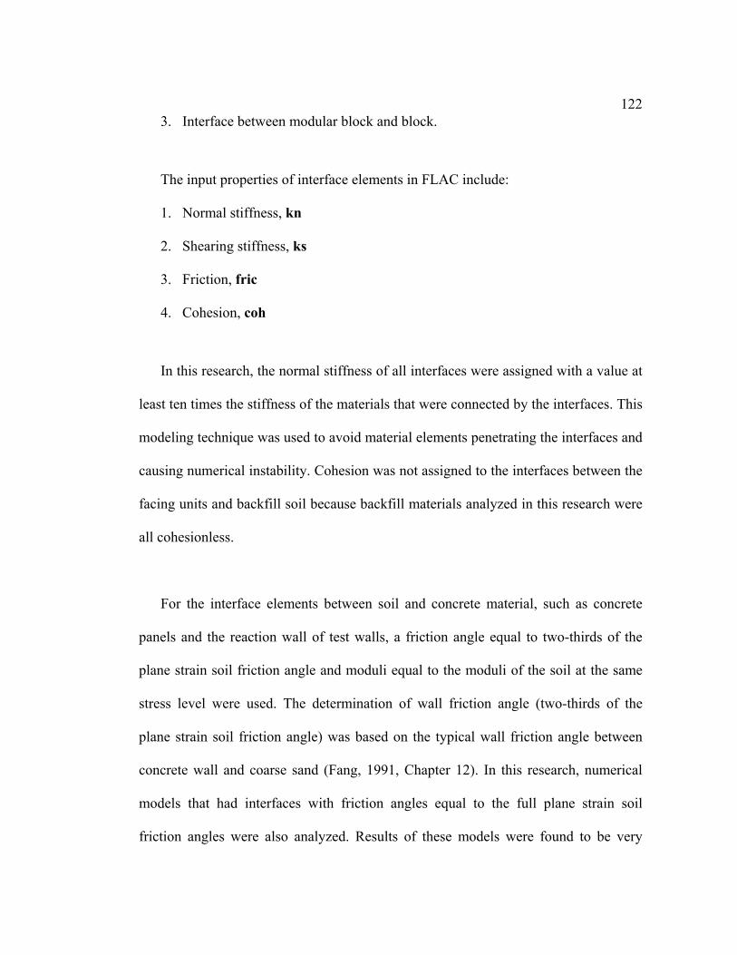
1223. Interface between modular block and block.
The input properties of interface elements in FLAC include:
1. Normal stiffness, kn
2. Shearing stiffness, ks
3. Friction, fric
4. Cohesion, coh
In this research, the normal stiffness of all interfaces were assigned with a value at
least ten times the stiffness of the materials that were connected by the interfaces. This
modeling technique was used to avoid material elements penetrating the interfaces and
causing numerical instability. Cohesion was not assigned to the interfaces between the
facing units and backfill soil because backfill materials analyzed in this research were
all cohesionless.
For the interface elements between soil and concrete material, such as concrete
panels and the reaction wall of test walls, a friction angle equal to two-thirds of the
plane strain soil friction angle and moduli equal to the moduli of the soil at the same
stress level were used. The determination of wall friction angle (two-thirds of the
plane strain soil friction angle) was based on the typical wall friction angle between
concrete wall and coarse sand (Fang, 1991, Chapter 12). In this research, numerical
models that had interfaces with friction angles equal to the full plane strain soil
friction angles were also analyzed. Results of these models were found to be very

123similar to models that used two-thirds of the plane strain soil friction angles as the
interface friction angles.
Modular block facing systems are more flexible than concrete panel systems.
Moreover, modular block facing systems have increased interaction with the backfill
because the blocks are usually set up with a certain setback between blocks that forms
a stepped contact surface between blocks and the backfill soil. Therefore properties of
interfaces between modular blocks and soil are expected to be different than the
interface properties of concrete panel facing systems. Burgess (1999) back-calculated
the vertical drag forces measured at the bottom of large scale GRS test walls and
found that the soil friction was fully mobilized behind the modular block facing. For
the interfaces between soil and modular block facing, a full friction angle equal to the
plane strain soil friction angle and moduli equal to the moduli of the soil at the same
stress level were used.
Properties of interface between block and block are really not easy to characterize
because different manufacturers develop different connection systems for their
products. Interface characteristics of blocks are also affected by the geosynthetic
reinforcements inserted between the blocks. There are three basic types of the block
connections:

1241. Friction connection – the connection relies on the friction between the block
material and gravel material filled in the blocks. Interface properties of this
type of connection are assumed to be the friction angle and shearing stiffness
of the gravel material.
2. Steel pin connection – steel pins are inserted in between the blocks to help
maintain the alignment of the blocks as well as to attach the reinforcement to
the facing units. Interface properties of this type of connection are assumed to
be the friction angle and shearing stiffness of the gravel infill material. The
existence of the steel pin of this type of connection can be simulated by
cohesion at the interface. The cohesion value can be obtained by dividing the
yield strength of the steel pin by the area of the blocks. However, the
difference between models with and without cohesion was found to be very
minor. This observation indicates that because the cross sectional area of the
pins is small, this type of block facing system still relies mainly on the friction
of the block material and the gravel material filled in the blocks.
3. Wedge connection – blocks of this type of connection system are made with a
convex wedge at one contact face and a compatible concave groove at the
other. This wedge design provides a very stiff connection because the
connection not only relies on the friction of the infill gravel material but also
on the strength of the block material. Friction of this type of connection is
assumed to be the friction angle of the gravel material. The shearing stiffness

125of the interface is calculated using Equation 8.5.1. The cohesion of the
interface is assumed to be the apparent cohesion of the block material.
bbgg REREks ⋅+⋅= (Eq. 8.5.1)
where ks = shearing stiffness of the interface,
Eg = stiffness of the gravel material,
Rg = coverage ratio of the gravel material =total
g
AA
,
Ag = cross sectional area occupied by the gravel material,
Atotal = total cross sectional area of the block unit,
Eb = stiffness of the block material,
Rb = coverage ratio of the block material =total
b
AA
, and
Ab = cross sectional area occupied by the block material.
8.5.9 Wall Construction
Field observations (instrumentation measurements) obtained from the case histories
analyzed in this research (Chapter 9), as well as the excellent performance of GRS
walls built as early as 1970s, indicate that most of the wall deflection occurs during
the wall construction, especially in well-designed GRS walls. Due to the conservative
nature of present design methods, these walls are so strong that almost no additional
deflections have been observed after construction. Deflections mostly occurred during
construction because soil moduli are relatively small when soil is first placed on each
lift of construction. Soil moduli increase as the confining pressure increases, i.e. as the

126height of the wall increases. Therefore, modeling the construction procedures and the
change of soil moduli caused by this confining pressure change are very important.
Modeling techniques used to account for the change of soil moduli due to confining
pressure change have been described in Section 8.5.4. GRS wall construction
procedures can be modeled as follows (Figure 8.5.4):
1. Place backfill soil (Mohr-Coulomb) and facing (elastic) elements of first layer.
2. Insert the interface between the soil and facing elements.
3. Place reinforcement (cable) elements.
4. Place backfill soil (Mohr-Coulomb) and facing (elastic) elements of next layer.
5. Insert the interface between the soil and facing elements, including interfaces
between facing elements of different layers, if any.
6. Solve the model to intermediate equilibrium state (intermediate equilibrium
criteria: srat=0.01), and
7. Repeat steps 3 to 6 until the wall is completed.
It is strongly recommended that the iteration result of construction of each lift be
saved, i.e. save each immediate and final stages, so that the development of the
working stress and strain of the modeling object can be monitored throughout the
construction simulations.
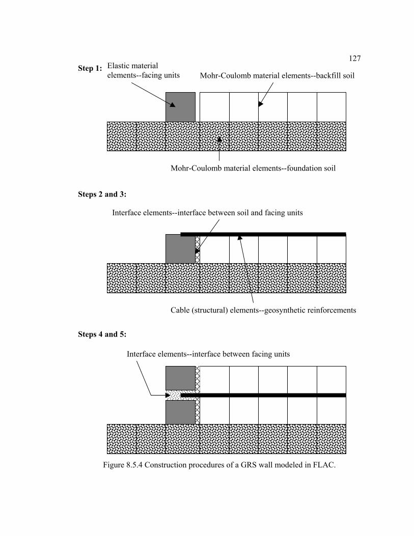
127Step 1:
Steps 2 and 3:
Steps 4 and 5:
Figure 8.5.4 Construction procedures of a GRS wall modeled in FLAC.
Cable (structural) elements--geosynthetic reinforcements
Interface elements--interface between facing units
Interface elements--interface between soil and facing units
Mohr-Coulomb material elements--backfill soilElastic material elements--facing units
Mohr-Coulomb material elements--foundation soil
1288.5.10 Modeling Result and Data Reduction
When FLAC models reach equilibrium at their final stages, displacement, stress and
strain of each material element as well as the axial forces of reinforcement element are
obtained directly from the saved result files. This information is either printed out as
data files or shown on the screen directly. The high stress-strain zone of the analyzed
walls can be located by showing the yielding (elastic or plastic) states of the material
elements. To ensure accuracy of the modeling results, the following issues were
checked:
1. That the equilibrium criteria were actually reached. Sometimes the iteration
process was stopped because the limit of the number of iterations was reached
before the stress ratio limit, but the modeling result had not converged.
2. That there were no notable displacements or reaction forces at the boundaries.
3. That strain compatibility is satisfied at every material element, i.e. that there is
no overlap or penetration of any adjacent material elements.
The horizontal displacement of the first column of material elements was used to
represent the wall face deflections. The horizontal stress distribution of this column
was also used to represent the distribution of the lateral reinforced earth pressures.
Strain distribution along the reinforcements was obtained by dividing the axial loads
of reinforcement with the tensile moduli of the reinforcements.

1298.6 Conclusions
Modeling techniques used to predict performance of the GRS retaining structures
appear to be very complicated, especially when structural facing systems are involved.
Modeling techniques described in Section 8.5 were obtained from numerous trials and
elaborate model calibrations. They provided the basic concepts and the specific
procedures to improve the working stress analyses of GRS retaining structures using
FLAC. Prerequisites for using these modeling techniques are a good understanding of
the in-structure material properties. Properties of both soil and geosynthetic
reinforcement have to be carefully determined as described in Chapter 7.

130Chapter 9
Verification of Numerical Modeling Techniques – Reproducing the
Performance of Existing GRS walls
9.1 Introduction
Performance data from four instrumented GRS retaining structures and two steel
reinforced retaining structures were collected to verify the numerical modeling
techniques described in Chapter 8. These case histories were chosen because they
were fully instrumented during construction and the results of the instrumentation
were well documented. These case histories include the WSDOT geotextile wall at the
west-bound I-90 preload fill in Seattle, Washington, and five of the test walls
constructed at the FHWA Reinforced Soil Project site at Algonquin, Illinois (Table
9.1.1).
Numerous trial models and much arduous work were done to develop models for these
case histories, as well as to calibrate these models to the latest modeling techniques. In
this chapter, results of six FLAC models that were developed to model the
performance of the case histories are presented and compared to the field
measurements. These FLAC models were developed following the same property
determination procedures and numerical modeling techniques described in Chapters 7
and 8, and they were able to reproduce the field performance of the analyzed case
histories within a reasonable range.

131Table 9.1.1 Summary of the numerical models of case histories.
Case History Model Name
WSDOT Rainier Avenue Geotextile Wall
Seattle, Washington
(Allen et al., 1992)
(12.6m high with 32 woven geotextile reinforcement
layers)
RAING
ALGPC1
(Wall 1: steel strips)
ALGPC2
(Wall 2: geogrid)
FHWA Algonquin Precast Concrete Panel Faced Test
Walls
Algonquin, Illinois
(Christopher, 1993)
(6.1m high with 8 reinforcement layers)
ALGPC3
(Wall 3: steel bar mats)
FHWA Algonquin Modular Block Faced Test Wall
Algonquin, Illinois
(Christopher, 1993)
(6.1m high with 8 geogrid reinforcement layers, uneven
vertical spacing)
ALGMB1
FHWA Algonquin Geotextile Wrapped Faced Test Wall
Algonquin, Illinois
(Christopher, 1993)
(6.1m high with 7 primary and 6 secondary nonwoven
reinforcement layers)
ALGWF1

1329.2 Summary of the Case Histories and Their Numerical Models
9.2.1 WSDOT Rainier Avenue Geotextile Wall
The first FLAC GRS wall model of this research was developed to predict the
instrumentation measurements of the WSDOT Rainier Avenue wall built in Seattle,
Washington. It was the highest GRS wall in the world at the time it was constructed.
The wall was 12.6 m high and had a surcharge of 5.3 m high with 1V: 1.8H slope. No
structural facing system was used for this wall; geotextiles were wrapped around the
wall face. Four different kinds of woven geotextiles were used to reinforce the backfill
of this wall (Christopher et al., 1990, Allen et al., 1992).
Figure 9.2.1 shows a typical cross-section with material properties of this wall.
Deflections of the wall were measured using optical surveys, photogrammetry, and
mechanical extensometer plate surveys at the wall face and inclinometers at the wall
face and 2.75 m behind the wall face. The internal strain distribution was measured
using strain gages and extensometers attached to the geosynthetic reinforcement.
Figure 9.2.2 shows the instrumented wall section of the Rainier Avenue wall (from
Allen et al., 1992).

133
Reinforcement:
Zone Geotextile Tult (kN/m) J (kN/m) 1 GTF200 (PP) 31 102 2 GTF375 (PP) 62 204 3 GTF5500 (PP) 92 357 4 GTF1225T (PET) 186 1125
Figure 9.2.1 Typical cross section of Rainier Avenue Geotextile wall (After Allen,
1999).
Foundation soil consists of 6m of dense gravelly sand underlain by 1 to 3 m of soft clayey silt, which is underlain by very dense gravelly sand
11.85 m
9.75 m
5.3 m
0.75 m
1V:1.8H Average
0.9 m
3.6 m Zone 1
3.05 m Zone 2
3.05 m Zone 3
2.9 m Zone 4
GeotextileWrapped Face
Backfill Soil: φtx = 45o, φps = 54o γ = 21.1 kN/m3 Sv = 0.38 m for all layers
1V:20H
PP: Polypropylene PET: Polyester
134The FLAC model, Model RAING, was developed for simulating the performance
of the Rainier Avenue Wall. In Model RAING, the soil moduli were determined using
the modified hyperbolic soil modulus model. Model parameters were determined
based on the triaxial test data with plane strain modifications, as described in Chapter
7. During the iteration process, soil moduli were automatically updated by the FISH
subroutine that was embedded in the FLAC model. Details of the FISH subroutine
were presented in Section 8.5.1. Input properties of the reinforcement were determined
using procedures described in Example 8.5.2 with an assumption of in-soil
reinforcement thickness equal to 5mm. The reinforcement (cable) elements were hard
tied onto the material element nodes, i.e. perfect bonding between the reinforcement
(cable) and soil (Mohr-Coulomb) elements was imposed. As described in Chapter 8,
this technique was used to avoid the violation of strain compatibility when large
deformations occurred in the models. Table 9.2.1 lists the input properties of Model
RAING.
9.2.2 Algonquin Precast Concrete Panel Faced Walls
The second set of FLAC wall models were developed to predict the performance data
of the Federal Highway Administration (FHWA) test walls built at Algonquin, Illinois.
These test walls were constructed as part of a FHWA study to investigate the behavior
of mechanically stabilized earth (MSE) walls (Christopher, 1993). Three of these walls
used the same type of wall facing, the cruciform precast concrete panels of the

135
Figure 9.2.2 Instrumented wall section of Rainier Avenue wall (after Allen et al., 1992).

136Reinforced Earth Company design, and each was reinforced with different
reinforcement materials. Two were reinforced using steel reinforcements and the other
was reinforced with geogrids. Table 9.2.2 summarizes the reinforcement types and
properties used in each wall. Figure 9.2.3 shows the wall geometry, material properties,
and instrumentation details for the geogrid wall (Wall 2). The wall geometry was
identical for Walls 1, 2 and 3, and the instrumentation details were similar. Backfill
material was a well-graded sand and gravel (Figure 9.2.3). The performance of all
three concrete panel walls was measured using inclinometers and surface optical
surveys for deflections, and strain gages and extensometers for internal strain
distributions. In this research, numerical models were first developed to simulate the
instrumentation measurements of the geogrid reinforced wall, Wall 2. Walls 1 and 3
were used as verifying cases in the parametric study. Results of the parametric study
are described in Chapter 12.
Models ALGPC1, ALGPC2, and ALGPC3 are the final models that were
developed by following the modeling techniques described in Chapter 8. Similar to
Model RAING, soil moduli for these models were also updated automatically using
the hyperbolic soil modulus model and the reinforcement elements were also attached
to the material element nodes. Input properties of the reinforcement were determined
by using procedures described in Example 8.5.2 with a assumption of in-soil
reinforcement thickness equal to 5 mm. Interface elements were inserted in between
the concrete panel (elastic material elements) and the backfill soil (Mohr-Coulomb

137
Table 9.2.1 Input properties of Model RAING.
Input Property Model RAING
Soil Friction Angle 50 deg
Soil Dilation Angle 15 deg
Soil Cohesion 0 kPa
Soil Moduli Automatically updated using modified hyperbolic soil modulus model
(K=1800, Rf=0.73, n=0.5) Reinforcement – GTF 200 E = 20300 kN/m2
Yield = 31 kN, Ycomp = 0
Reinforcement – GTF 375 E = 40800 kN/m2
Yield = 62 kN, Ycomp = 0
Reinforcement – GTF 500 E = 71300 kN/m2
Yield = 92 kN, Ycomp = 0
Reinforcement – GTF 1225T E = 225000 kN/m2
Yield = 186 kN, Ycomp = 0
Table 9.2.2 Construction and reinforcement information of the Algonquin concrete
panel faced walls (Christopher, 1993). Wall Names Wall 1 Wall 2 Wall 3
Reinforcement Name and Type
Reinforced Earth Company—Ribbed Steel Strips
Tensar SR2—Polyethylene Extruded Geogrids
VSL—Steel Bar Mats using W11 Bars
Reinforcement Strength, Strain, and Stiffness
Tyield= 67.9kN/m a
εyield=0.12%
J=54690kN/m a
Tpeak= 67.7kN/m b
εpeak=16.0%
J=2040kN/m b
Tyield= 44.4kN/m a
εyield=0.12%
J=37860kN/m a a per meter of wall, calculated based on the coverage ratio (the width of the
reinforcement divided by the center to center horizontal spacing). b from wide width strip tensile tests (ASTM D 4595)
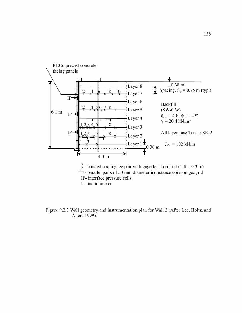
138
6.1 m
RECo precast concretefacing panels
4.3 m
Backfill:(SW-GW)φtx = 40o , φps = 43o
γ = 20.4 kN/m3
All layers use Tensar SR-2
Spacing, Sv = 0.75 m (typ.)0.38 m
0.38 m
Layer 8Layer 7
Layer 6
Layer 5
Layer 4
Layer 3
Layer 2
Layer 1
x x x x x x
x x x x x x x
x x x x x x x
I I
x x x x x x
x x x
2 4 6 8 10
2 4 5 6 7 8
1 2 3 4 5 8
1 2 3 5 8
1 3
IP
IP
IP
x - bonded strain gage pair with gage location in ft (1 ft = 0.3 m) - parallel pairs of 50 mm diameter inductance coils on geogridIP- interface pressure cellsI - inclinometer
2
Figure 9.2.3 Wall geometry and instrumentation plan for Wall 2 (After Lee, Holtz, and
Allen, 1999).
J2% = 102 kN/m

139material elements). As stated in Chapter 8, for the interface elements between soil and
concrete panels, a friction angle equal to two-thirds of the plane strain soil friction
angle and stiffness equal to the average stiffness of the soil behind the wall face were
used. Table 9.2.3 lists the input properties of these models.
9.2.3 Algonquin Modular Block Faced Wall
FLAC models were also developed to simulate the performance of the geogrid
reinforced modular block faced wall of the FHWA Algonquin test walls, in order to
calibrate the developed modeling techniques for different MSE wall facing systems.
Figure 9.2.4 shows the typical cross section and material properties of the modular
block faced wall. As shown in Figure 9.2.4, vertical spacings of the reinforcement
layers were varied throughout the wall height in an attempt to “amplify” the face
deformation as well as the internal strain levels of the wall. wall (after Bathurst et. al.,
1993). The wall was designed to have the largest spacing at two-thirds of the wall
height where the maximum wall deflection was expected to occur. Deflections of the
wall were measured using inclinometers at the wall face and 2.7 m behind the wall
face. The internal strain distribution was measured using strain gages attached to the
geogrids reinforcements. Figure 9.2.5 shows the instrumentation wall section of this
wall (Bathurst et al., 1993).

140Table 9.2.3 Input properties of Models ALGPC1, ALGPC2, and CLGPC3.
Input Property
Model ALGPC1
Model ALGPC2
Model ALGPC3
Soil Friction Angle 43 deg
Soil Dilation Angle 15 deg
Soil Cohesion 0 kPa
Soil Moduli Automatically updated using hyperbolic soil modulus model
(K=1100, Rf=0.73, n=0.5)
Interface kn = 373000 kN/m2, ks = 187000
kN/m2, fric = 28.7, coh = 0,
Ribbed Steel Strip
Wall 1
Model ALGPC1
E = 1.2E7 kN/m2
Yield = 1E6 kN,
Ycomp = 1E6 kN.
Geogrid
Wall 2
Model ALGPC2
E = 204000 kN/m2
Yield = 67.8 kN,
Ycomp = 0.
Steel Bar Mat
Wall 3
Model ALGPC3
E = 8.0E6 kN/m2
Yield = 1E6 kN,
Ycomp = 1E6kN.
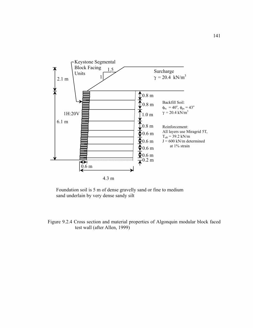
141
Figure 9.2.4 Cross section and material properties of Algonquin modular block faced test wall (after Allen, 1999)
Backfill Soil: φtx = 40o, φps = 43o γ = 20.4 kN/m3 Reinforcement: All layers use Miragrid 5T,Tult = 39.2 kN/m J = 600 kN/m determined
at 1% strain
Keystone SegmentalBlock Facing Units
11.5
1H:20V
Foundation soil is 5 m of dense gravelly sand or fine to medium sand underlain by very dense sandy silt
6.1 m
2.1 m
0.6 m
4.3 m
Surcharge γ = 20.4 kN/m3
0.8 m
0.8 m
0.8 m
1.0 m
0.6 m
0.6 m0.6 m
0.6 m
0.2 m

142
Figure 9.2.5 Instrumentation section of the Algonquin modular block faced geogrid

143FLAC model ALGMB1 was developed to model the performance of this wall.
Model ALGMB1 was developed utilizing the modeling techniques described in
Chapter 8, such as using the hyperbolic soil modulus models and attaching
reinforcement elements to the material element nodes. In Model ALGMB1, the
modulus of the geogrid reinforcement was the tangent modulus determined at 1%
strain with in-soil and low strain rate modification because the average reinforcement
strain measured by the strain gages was less than 1%. The in-soil reinforcement
thickness was assumed to be 5 mm similar to other cases. Moreover, the stiffness that
was determined from connection test data (Bathurst, 1999) was used as the modulus of
the reinforcement located inside the blocks. In Model ALGMB1, effort was also made
to model the block facing system including the interfaces between blocks as well as
the gravel column behind the modular block face. The purpose of placing this gravel
column was to maintain good drainage and thus reduce excessive water pressure on
the wall face. However, properties of the interfaces between blocks and the gravel
material were not clearly described in the documentation (Bathurst et al, 1993). Table
9.2.4 lists the input properties of Model ALGMB1, most of which were determined
from manufacturer’s information.
9.2.4 Algonquin Wrapped Face Wall
FLAC models were also developed to reproduce the performance of the wrapped face
wall of FHWA Algonquin test walls because the poor design of this wall allowed large
strains to occur. The test wall was designed with a very weak nonwoven geosynthetic

144as reinforcement and a 1 m high surcharge on the top. Secondary reinforcement layers,
additional horizontal reinforcement, were inserted near the face of the wall to increase
the stability of the face. A water pond built with an impermeable membrane was also
placed in front of the wall to help maintain the stability of the wall during surcharge
construction. Figure 9.2.6 shows the typical cross section and material properties of
the wrapped face wall. This retaining water pond was then removed after the wall was
completed to observe the possible failure of this GRS wall. Similar instrumentation to
the other Algonquin test walls was used to monitor the performance of this wrapped
face wall. Figure 9.2.7 shows the instrumentation section of this wall. However,
optical survey and inclinometer measurements of wall deflection were not available
because of the retaining water pond in front of the wall and the gabion basket
surcharge on the top of the wall (Christopher 1993).
FLAC model ALGWF1 was developed using similar modeling techniques to those
used in Model RAING. The average measured reinforcement strain inside the wrapped
face wall was less than 2%. However, there was only an in-soil stiffness obtained from
pull-out test at 12% strain available in the documentation (Christopher, 1993). In
Model ALGWF1, the reinforcement stiffness was determined using in-isolation test
data of reinforcing material similar to what was used in this test wall. The input
stiffness of the reinforcement was determined by multiplying the 2% strain in-isolation
stiffness by five, a modification based on the UCD test results reported by Boyle
(1995). Additional effort was also made to model the completed boundary conditions
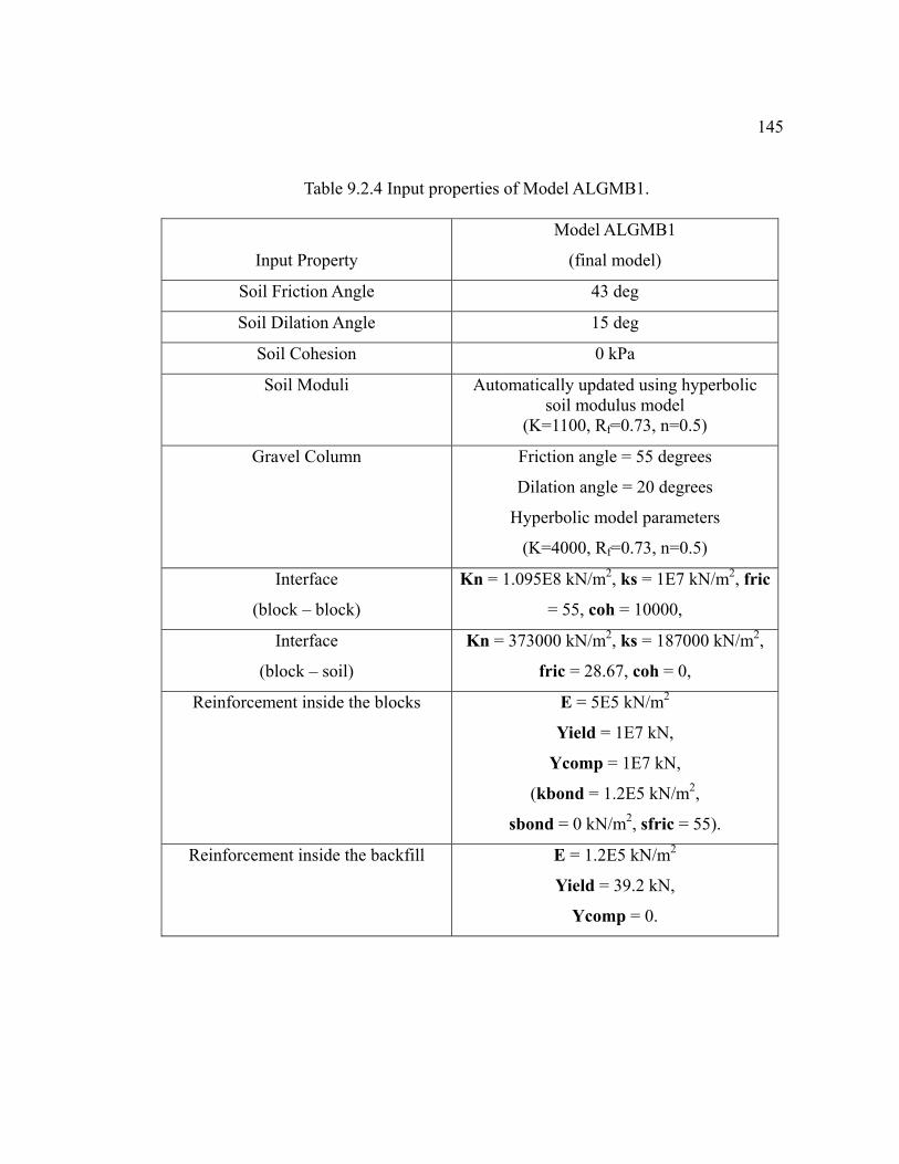
145
Table 9.2.4 Input properties of Model ALGMB1.
Input Property
Model ALGMB1
(final model)
Soil Friction Angle 43 deg
Soil Dilation Angle 15 deg
Soil Cohesion 0 kPa
Soil Moduli Automatically updated using hyperbolic soil modulus model
(K=1100, Rf=0.73, n=0.5)
Gravel Column Friction angle = 55 degrees
Dilation angle = 20 degrees
Hyperbolic model parameters
(K=4000, Rf=0.73, n=0.5)
Interface
(block – block)
Kn = 1.095E8 kN/m2, ks = 1E7 kN/m2, fric
= 55, coh = 10000,
Interface
(block – soil)
Kn = 373000 kN/m2, ks = 187000 kN/m2,
fric = 28.67, coh = 0,
Reinforcement inside the blocks E = 5E5 kN/m2
Yield = 1E7 kN,
Ycomp = 1E7 kN,
(kbond = 1.2E5 kN/m2,
sbond = 0 kN/m2, sfric = 55).
Reinforcement inside the backfill E = 1.2E5 kN/m2
Yield = 39.2 kN,
Ycomp = 0.
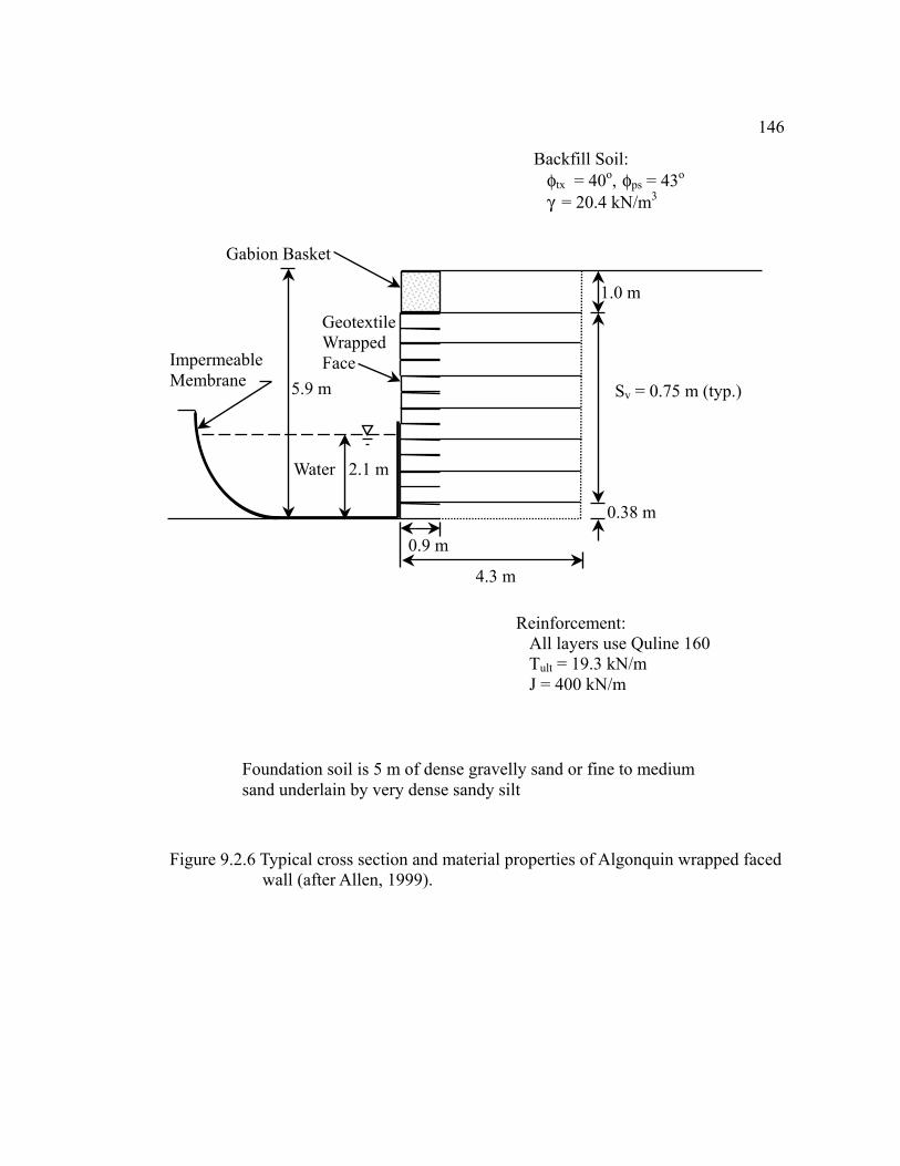
146
Figure 9.2.6 Typical cross section and material properties of Algonquin wrapped faced
wall (after Allen, 1999).
5.9 m
2.1 m
4.3 m
0.9 m
Water
Backfill Soil: φtx = 40o, φps = 43o γ = 20.4 kN/m3
Impermeable Membrane
GeotextileWrapped Face
Gabion Basket
Foundation soil is 5 m of dense gravelly sand or fine to medium sand underlain by very dense sandy silt
Sv = 0.75 m (typ.)
0.38 m
1.0 m
Reinforcement: All layers use Quline 160 Tult = 19.3 kN/m J = 400 kN/m

147
Figure 9.2.7 Instrumentation section of the Algonquin wrapped faced wall (After
Christopher, 1993).

148of this wall. The retaining water pond was modeled using elastic material elements
with density equal to 1 and Poisson’s ratio equal to 0.5. The gabion baskets were
modeled by wrapping the Mohr-Coulomb material element (properties of gravel were
assigned) with cable elements with properties of steel wires. Table 9.2.5 lists the input
properties of Model ALGWF1.
In the following sections, performance predictions of the developed models of the
case histories described above are presented. In Section 9.3, deflection predictions of
the developed wall models are presented and compared to the optical survey or
inclinometer measurements. In Section 9.4, predictions of the reinforcement strain
distributions of these models are also presented and compared to the strain gage
measurement as well as the extensometer measurements if available. Finally, the
reinforcement tension distributions obtained from the numerical models are presented
in Section 9.5 to compare with the predictions made by the tie-back wedge method.

149Table 9.2.5 Input properties of Model ALGWF1.
Input Property Model ALGWF1
Soil Friction Angle 43 deg
Soil Dilation Angle 15 deg
Soil Cohesion 0 kPa
Soil Moduli Automatically updated using hyperbolic soil modulus model
(K=1100, Rf=0.73, n=0.5)
Gabion Basket Gravel:
Den=2.4 fric=50 di=10 coh=35
Steel wire:
E=175e3 yield=200 kN ycomp=200
kN sbond=0 kbond=175e3
sfric=50
Reinforcement
At face (in-isolation)
E = 1.6E4 kN/m2
Yield = 19.3 kN,
Ycomp = 0
Reinforcement
In backfill (in soil)
E = 8E4 kN/m2
Yield = 19.3 kN,
Ycomp = 0,

1509.3 Modeling Results I—Wall Deflection
9.3.1 WSDOT Rainier Avenue Wall
Figures 9.3.1a and 9.3.1b show the face deflection results of Model RAING compared
with the average survey measurements of the WSDOT Rainier Avenue wall at end of
the construction and after surcharge. Average deflection survey measurements were
used to eliminate errors between different survey measurements. Model RAING was
able to predict reasonable face deflections and the locations where the maximum
deflection was observed. As shown in Figure 9.3.1, Result of Model RAING under-
predicts the wall face deflection by only about 20 mm at end of construction and over-
predicts the wall deflection by only about 10 mm after surcharge applied for the 12.6
m high wrapped face wall.
Similar tendencies were also found when comparing the modeling results to the
measurements of the inclinometer located at 2.75 m behind the wall face (Figures
9.3.2a and 9.3.2b). As shown in Figure 9.3.2a, Model RAING under-predicted the wall
deformation by less than 10 mm at the elevation where maximum face deformation
was observed (Figure 9.3.1) at end of construction. After surcharge is applied, result of
Model RAING also had a very good agreement to the inclinometer measurements
below the elevation where maximum wall face deflection was observed. It only
slightly under-predicts the deformation by 10 mm at the elevation where maximum
face deflection was observed.
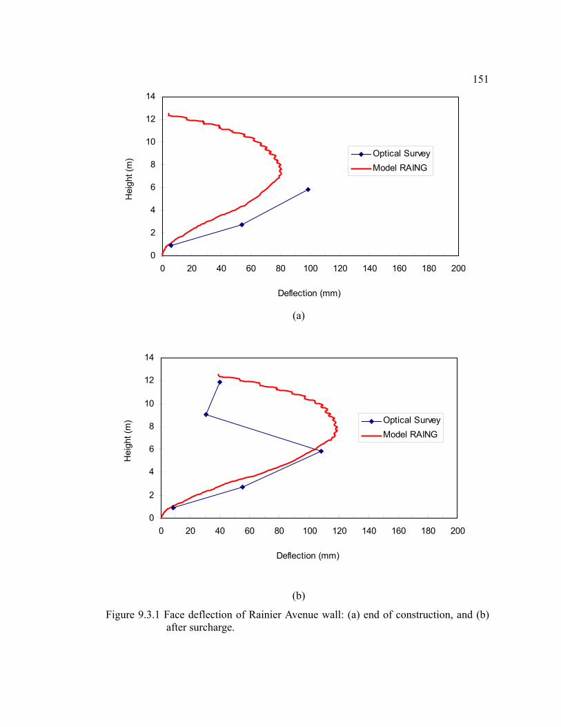
151
(a)
(b)
Figure 9.3.1 Face deflection of Rainier Avenue wall: (a) end of construction, and (b) after surcharge.
0
2
4
6
8
10
12
14
0 20 40 60 80 100 120 140 160 180 200
Deflection (mm)
Hei
ght (
m) Optical Survey
Model RAING
0
2
4
6
8
10
12
14
0 20 40 60 80 100 120 140 160 180 200
Deflection (mm)
Hei
ght (
m) Optical Survey
Model RAING
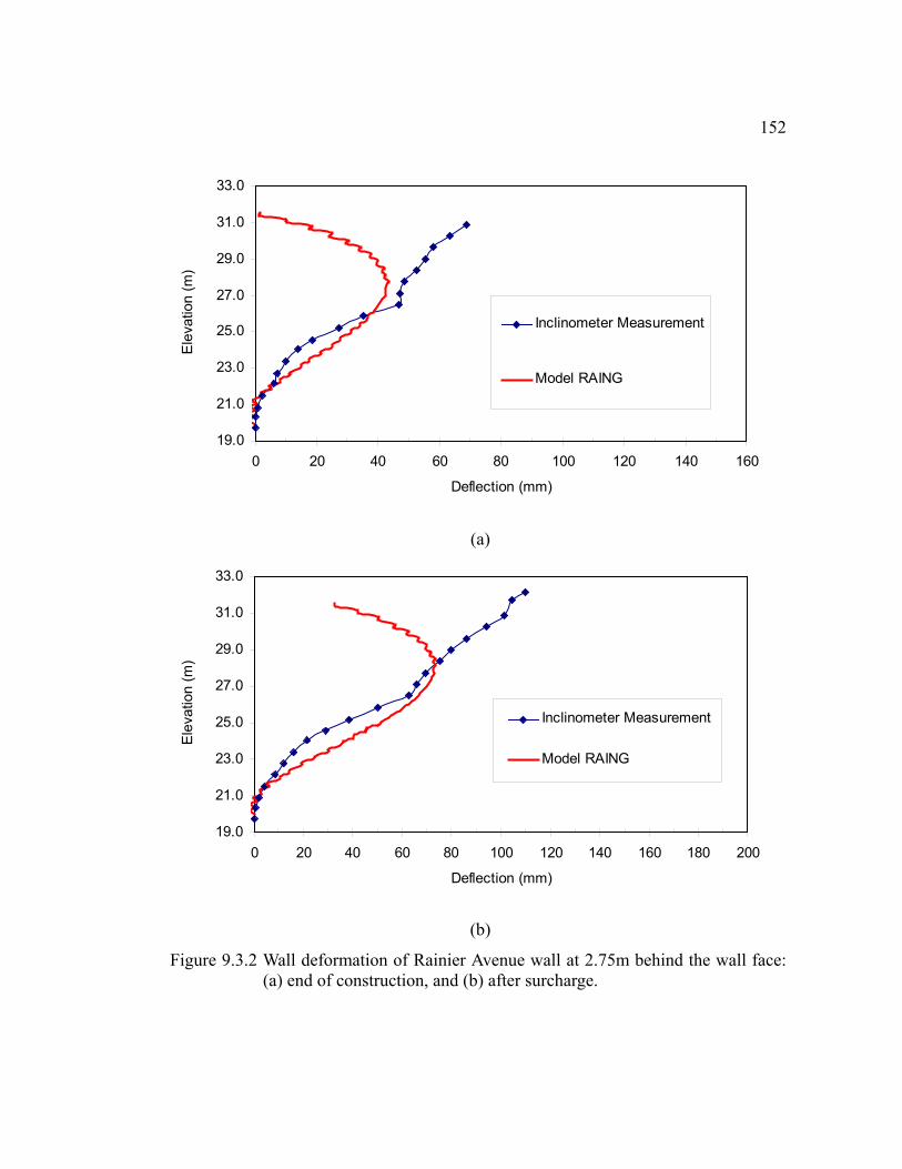
152
(a)
(b)
Figure 9.3.2 Wall deformation of Rainier Avenue wall at 2.75m behind the wall face: (a) end of construction, and (b) after surcharge.
19.0
21.0
23.0
25.0
27.0
29.0
31.0
33.0
0 20 40 60 80 100 120 140 160
Deflection (mm)
Elev
atio
n (m
)
Inclinometer Measurement
Model RAING
19.0
21.0
23.0
25.0
27.0
29.0
31.0
33.0
0 20 40 60 80 100 120 140 160 180 200
Deflection (mm)
Elev
atio
n (m
)
Inclinometer Measurement
Model RAING

153Modeling results shown in Figure 9.3.2 had different predictions from the
inclinometer measurements above the location where the maximum face deflection
occurred. Reasons why the inclinometer measurements showed a maximum wall
deflection at top of the wall are not clear at present.
9.3.2 Algonquin Concrete Panel Faced Walls
Model ALGPC2 was able to predict both the shape and maximum deflection of the
geogrid wall within reasonable agreement (Figure 9.3.3). As shown in Figure 9.3.3,
Model ALGPC2 under-predicts the maximum face deflection of the geogrid wall by
only about 5 mm. The results of Models ALGPC1 and ALGPC3 also showed
reasonable agreement with the behavior of the steel reinforced walls (Wall 1 and Wall
3) (Figures 9.3.4 and 9.3.5). Because of the high stiffness of the reinforcement of
Walls 1 and 3, the magnitudes of face deflections and the reinforcement strains are
very small. Thus the potential error in the measurements due to the accuracy of the
optical survey could be very close to the magnitude of the measurements themselves.
As shown in Figures 9.3.4 and 9.3.5, Models ALGPC1 and ALGPC3 predicted very
small survey face deflections, and the difference between predicted and measured
maximum deflection is only about 5 mm.

154
Figure 9.3.3 Predicted and measured wall face deflection of Algonquin concrete panel
faced Wall 2 (geogrid wall).
Figure 9.3.4 Predicted and measured wall face deflection of Algonquin concrete panel faced Wall 1 (steel strips wall).
0
1
2
3
4
5
6
0 10 20 30 40 50
Deflection (mm)
Hei
ght (
m)
Model ALGPC2
Survey at Face
0
1
2
3
4
5
6
0 10 20 30 40 50
Deflection (mm)
Hei
ght (
m)
Model ALGPC1
Survey at Face

155
Figure 9.3.5 Predicted and measured wall face deflection of Algonquin concrete panel
faced Wall 3 (steel bar mats wall).
0
1
2
3
4
5
6
0 10 20 30 40 50
Deflection (mm)
Hei
ght (
m) Model ALGPC3
Survey at Face

1569.3.3 Algonquin Modular Block Faced Wall
Model ALGMB1 was able to predict the instrumentation measurements within a
reasonable range. Figure 9.3.6 shows the prediction of Model ALGMB1 compared to
the measurements obtained from the inclinometer behind the wall face. Model
ALGMB1 tends to over-estimate the wall deflection at the location where maximum
face deflections were predicted by about 10 mm at the end of construction and by
about 25 mm after surcharge was applied. Possible reason for this over-estimation is
the input friction used for the interface between facing blocks was smaller than actual
fiction occurred in between the blocks of this wall.
Figure 9.3.7 shows the modeling result comparing to the measurements of the
inclinometer located 2.7 m behind the wall face. In Figure 9.3.7, “folds” or “jogs”
were observed on the predicted soil deflection curves. This is because soil elements
located next to reinforcement have a smaller deformation than the soil elements
located in between the reinforcement layers. Especially at the lower half of the wall,
jogs and folds in the modeling results become more obvious. As shown in Figure 9.3.7,
the average results of Model ALGMB1 had a reasonable agreement with the
inclinometer measurements at end of the construction in the bottom half of the wall. It
tended, however, to over-estimate the wall deflection by about 25 mm after surcharge
is applied.

157
(a) End of construction
(b) After surcharge
Figure 9.3.6 Predicted and measured wall face deflection of Algonquin modular block faced wall.
0
1
2
3
4
5
6
7
0 20 40 60 80 100
Deflection (mm)
Hei
ght (
m)
Model ALGMB1
Inclinometer Measurements
0
1
2
3
4
5
6
7
0 20 40 60 80 100
Deflection (mm)
Hei
ght (
m)
Model ALGMB1
InclinometerMeasurements
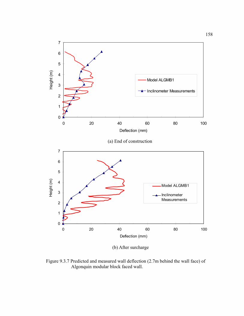
158
(a) End of construction
(b) After surcharge
Figure 9.3.7 Predicted and measured wall deflection (2.7m behind the wall face) of
Algonquin modular block faced wall.
0
1
2
3
4
5
6
7
0 20 40 60 80 100
Deflection (mm)
Hei
ght (
m)
Model ALGMB1
Inclinometer Measurements
0
1
2
3
4
5
6
7
0 20 40 60 80 100
Deflection (mm)
Hei
ght (
m)
Model ALGMB1
InclinometerMeasurements
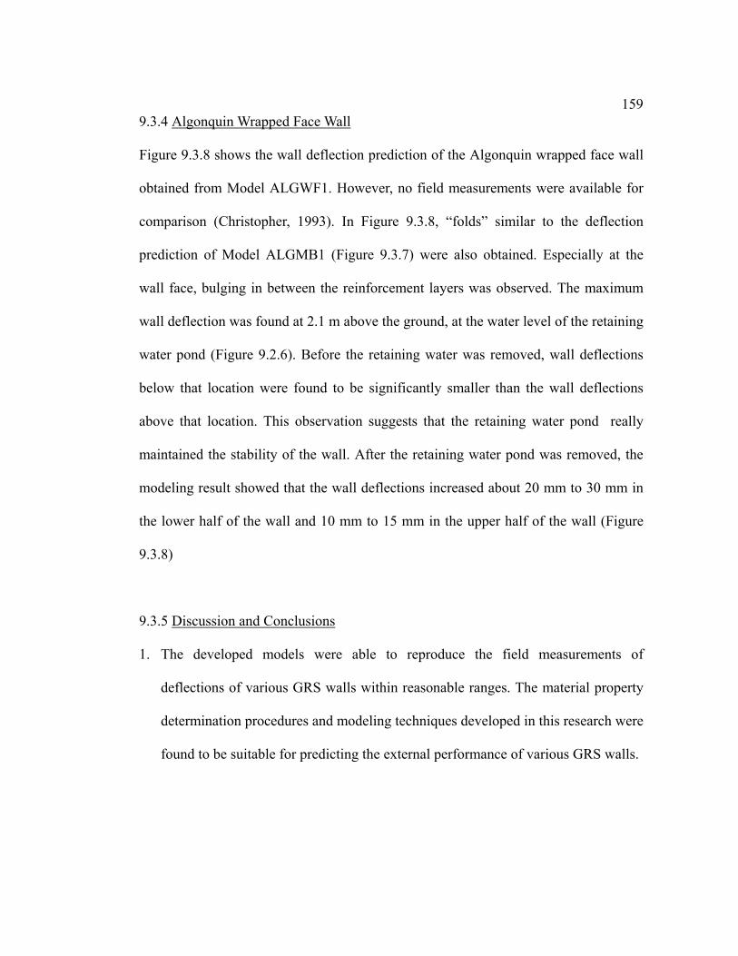
1599.3.4 Algonquin Wrapped Face Wall
Figure 9.3.8 shows the wall deflection prediction of the Algonquin wrapped face wall
obtained from Model ALGWF1. However, no field measurements were available for
comparison (Christopher, 1993). In Figure 9.3.8, “folds” similar to the deflection
prediction of Model ALGMB1 (Figure 9.3.7) were also obtained. Especially at the
wall face, bulging in between the reinforcement layers was observed. The maximum
wall deflection was found at 2.1 m above the ground, at the water level of the retaining
water pond (Figure 9.2.6). Before the retaining water was removed, wall deflections
below that location were found to be significantly smaller than the wall deflections
above that location. This observation suggests that the retaining water pond really
maintained the stability of the wall. After the retaining water pond was removed, the
modeling result showed that the wall deflections increased about 20 mm to 30 mm in
the lower half of the wall and 10 mm to 15 mm in the upper half of the wall (Figure
9.3.8)
9.3.5 Discussion and Conclusions
1. The developed models were able to reproduce the field measurements of
deflections of various GRS walls within reasonable ranges. The material property
determination procedures and modeling techniques developed in this research were
found to be suitable for predicting the external performance of various GRS walls.
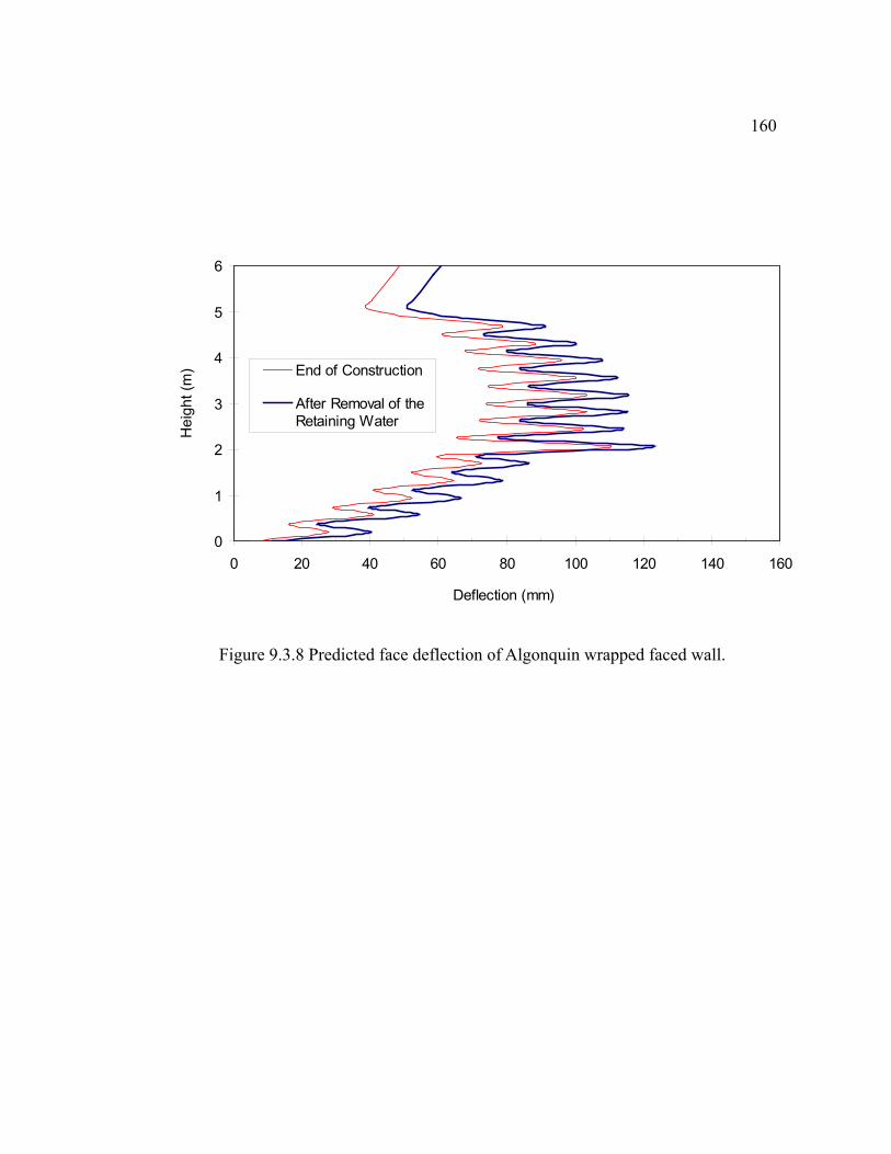
160
Figure 9.3.8 Predicted face deflection of Algonquin wrapped faced wall.
0
1
2
3
4
5
6
0 20 40 60 80 100 120 140 160
Deflection (mm)
Hei
ght (
m) End of Construction
After Removal of theRetaining Water

1612. Different predictions were found between the modeling results and inclinometer
measurements, especially above the locations of maximum wall deflections
predicted by the numerical models (Figures 9.3.2, 9.3.6, and 9.3.7). The
inclinometer measurements indicated a maximum wall deflection at the top of the
wall, while the modeling results indicated a maximum deflection at about two-
thirds height of the wall. A possible explanation is that the inclinometer tubing was
not perfectly bonded with the backfill soil, i.e. soil might move around the tubing.
To verify the difference between the inclinometer measurements and modeling
prediction, the internal strain and stress information such as reinforcement strain
distributions and reinforcement tension distributions obtained from both modeling
results and instrumentation measurements were analyzed to determine the actual
strain magnitudes that occurred in the upper one-third of these walls. Results of
these internal strain and stress analyses are presented in the following sections.
3. For GRS walls with complicated facing systems such as modular block facing,
accurate deflection predictions relied on not only correct input properties of soil
and geosynthetic, but also on the correct input properties of the interface between
blocks and reinforcements that were inserted in between the blocks. In Model
ALGMB1, input properties of the interfaces between blocks were determined
using the manufacturer’s information because actual material properties were not
reported in the references.

1624. Modeling results also show that soil elements located next to reinforcement layers
indicate smaller deformations than the soil elements located in between the
reinforcements. Especially at the bottom half of the GRS walls or at the face of the
wrapped face wall where no structural facing units are used to confine the bulges,
this interlayer reinforcing phenomenon becomes more obvious (Figures 9.3.7 and
9.3.8).

1639.4 Modeling Results II—Reinforcement Strain Distribution
9.4.1 WSDOT Rainier Avenue Wall
Figure 9.4.1 shows the strain distribution of the instrumented geosynthetic
reinforcement layers (Layers 4, 9, 17, and 26) of Model RAING compared with the
strain gage and extensometer measurements at end of construction. Layers 4, 9, 17,
and 26 were the instrumented layers of the four different reinforcement materials used
in the wall (Figure 9.2.2). Figure 9.4.2 is similar to Figure 9.4.1 but shows the
reinforcement strain distribution after surcharge was applied.
As shown in Figures 9.4.1 and 9.4.2, the results of Model RAING show excellent
agreement with instrumentation measurements of Layer 4, for both maximum strain
magnitudes and locations at end of construction and after surcharge.
Reinforcement strain distribution and magnitudes of Layer 9 were also
successfully reproduced by Model RAING. At the end of construction, Model RAING
was able to verify the maximum strain locations and the reinforcement strain
magnitudes of layer 9 (Figure 9.4.1). After surcharge, Model RAING tended to over-
predict the reinforcement strains by only 0.3% to 0.7% overall, yet it had very close
prediction of the location of the maximum reinforcement strain (Figure 9.4.1).
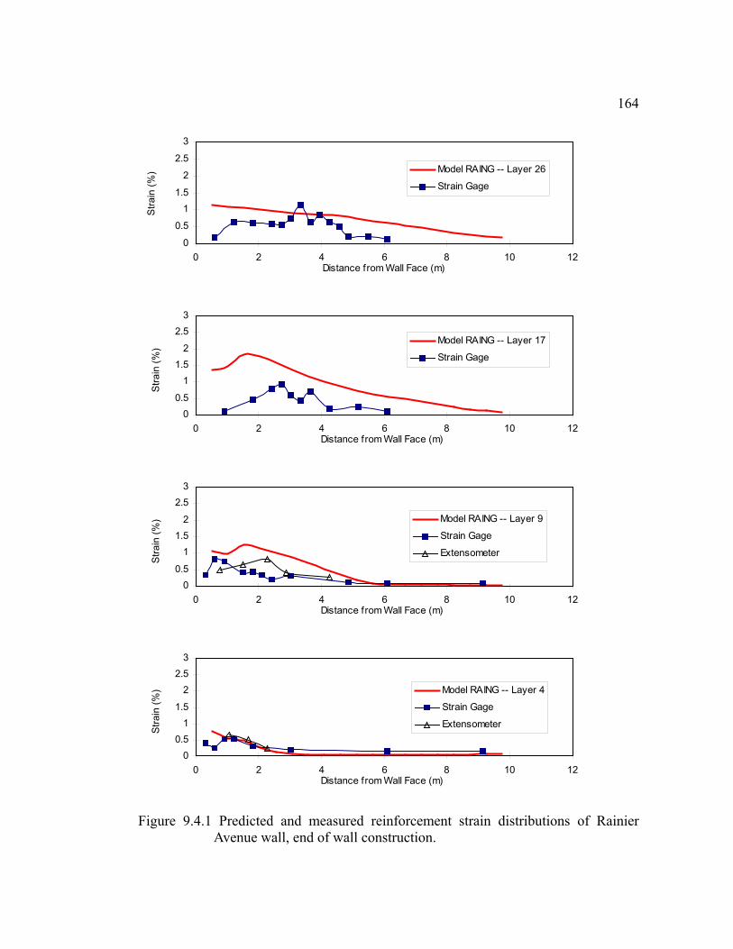
164
Figure 9.4.1 Predicted and measured reinforcement strain distributions of Rainier
Avenue wall, end of wall construction.
0
0.5
11.5
2
2.5
3
0 2 4 6 8 10 12Distance from Wall Face (m)
Stra
in (%
) Model RAING -- Layer 26
Strain Gage
00.5
11.5
2
2.53
0 2 4 6 8 10 12Distance from Wall Face (m)
Stra
in (%
)
Model RAING -- Layer 17
Strain Gage
00.5
11.5
2
2.53
0 2 4 6 8 10 12Distance from Wall Face (m)
Stra
in (%
) Model RAING -- Layer 9
Strain Gage
Extensometer
00.5
11.5
22.5
3
0 2 4 6 8 10 12Distance from Wall Face (m)
Stra
in (%
) Model RAING -- Layer 4
Strain Gage
Extensometer

165
Figure 9.4.2 Predicted and measured reinforcement strain distributions of Rainier
Avenue wall, after surcharge.
0
1
2
3
4
0 2 4 6 8 10 12Distance from Wall Face (m)
Stra
in (%
) Model RAING -- Layer 26
Strain Gage
0
1
2
3
4
0 2 4 6 8 10 12Distance from Wall Face (m)
Stra
in (%
)
Model RAING -- Layer 17
Strain Gage
0
1
2
3
4
0 2 4 6 8 10 12Distance from Wall Face (m)
Stra
in (%
) Model RAING -- Layer 9
Strain Gage
Extensometer
0
1
2
3
4
0 2 4 6 8 10 12Distance from Wall Face (m)
Stra
in (%
) Model RAING -- Layer 4
Strain Gage
Extensometer

166Model RAING tended to over-estimate the reinforcement strains at higher
elevations of the Rainier Avenue wall, and it predicted maximum strain locations
different from those observed by instrumentation measurements. However, the
differences between the prediction and instrumentation measurements are less than
1.5% of maximum strain magnitudes and within 0.5 m to 1.0 m of the location of the
maximum strain. For Layer 17, results of Model RAING showed a single peak strain
at 1.75 m behind the wall face with magnitudes of 1.8% at end of construction and
2.5% after surcharge (Figures 9.4.1 and 9.4.2). The measured peak strains were
located at 3m behind the wall face and had magnitudes of 1.0% at end of construction
and 1.2% after surcharge (Figures 9.4.1 and 9.4.2). Generally speaking, reinforcement
strain distributions predicted by Model RAING covered the measured distribution
reasonably well.
For Layer 26, as shown in Figures 9.4.1 and 9.4.2, Model RAING gave very good
predictions of magnitudes of the maximum reinforcement strains. However, different
from the instrumentation measurements which indicated a peak strain at 3.8 m behind
the wall face, Model RAING predicted the maximum reinforcement strain at the wall
face for both end-of-construction and after-surcharge stages. Possible reasons for the
difference is that, in Model RAING, the reinforcement elements were attached to the
material element nodes to avoid the violation of strain compatibility during iterations.
Reinforcement elements of Layer 26 at the wall face presented a maximum strain at
wall face because reinforcement strains inside the backfill were relatively small at this
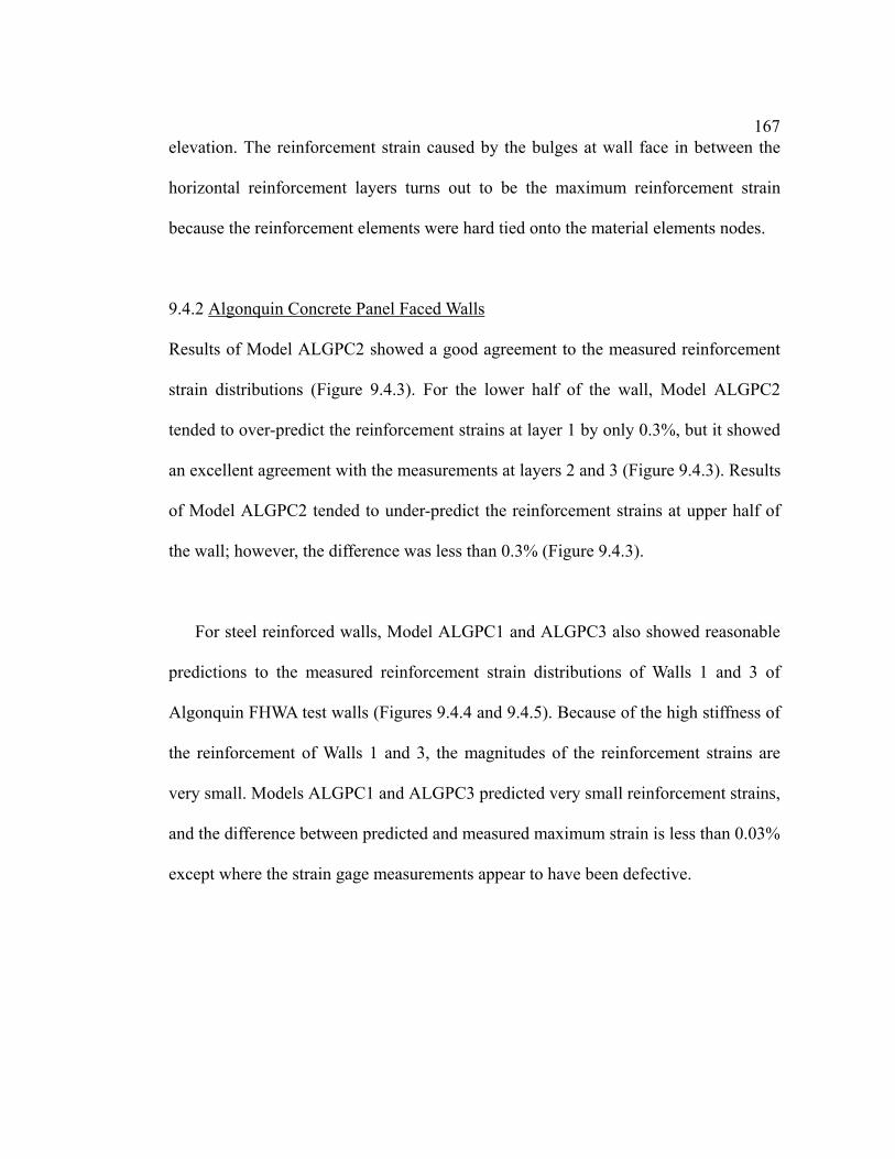
167elevation. The reinforcement strain caused by the bulges at wall face in between the
horizontal reinforcement layers turns out to be the maximum reinforcement strain
because the reinforcement elements were hard tied onto the material elements nodes.
9.4.2 Algonquin Concrete Panel Faced Walls
Results of Model ALGPC2 showed a good agreement to the measured reinforcement
strain distributions (Figure 9.4.3). For the lower half of the wall, Model ALGPC2
tended to over-predict the reinforcement strains at layer 1 by only 0.3%, but it showed
an excellent agreement with the measurements at layers 2 and 3 (Figure 9.4.3). Results
of Model ALGPC2 tended to under-predict the reinforcement strains at upper half of
the wall; however, the difference was less than 0.3% (Figure 9.4.3).
For steel reinforced walls, Model ALGPC1 and ALGPC3 also showed reasonable
predictions to the measured reinforcement strain distributions of Walls 1 and 3 of
Algonquin FHWA test walls (Figures 9.4.4 and 9.4.5). Because of the high stiffness of
the reinforcement of Walls 1 and 3, the magnitudes of the reinforcement strains are
very small. Models ALGPC1 and ALGPC3 predicted very small reinforcement strains,
and the difference between predicted and measured maximum strain is less than 0.03%
except where the strain gage measurements appear to have been defective.

168
Figure 9.4.3 Predicted and measured reinforcement strain distributions of Algonquin concrete panel faced wall, Wall 2 (geogrid reinforced).
0.00.51.0
1.52.0
0 0.5 1 1.5 2 2.5 3 3.5 4 4.5Distance from Wall Face (m)
Stra
in (%
)Layer 7 - Model ALGPC2
Strain Gage
0.0
0.5
1.0
1.5
2.0
0 0.5 1 1.5 2 2.5 3 3.5 4 4.5Distance from Wall Face (m)
Stra
in (%
)
Layer 5 - Model ALGPC2
Strain Gage
0.0
0.5
1.0
1.5
2.0
0 0.5 1 1.5 2 2.5 3 3.5 4 4.5Distance from Wall Face (m)
Stra
in (%
) Layer 3 - Model ALGPC2
Strain Gage
0.0
0.5
1.0
1.5
2.0
0 0.5 1 1.5 2 2.5 3 3.5 4 4.5Distance from Wall Face (m)
Stra
in (%
) Layer 2 - Model ALGPC2
Strain Gage
0.0
0.5
1.0
1.5
2.0
0 0.5 1 1.5 2 2.5 3 3.5 4 4.5Distance from Wall Face (m)
Stra
in (%
)
Layer 1 - Model ALGPC2
Strain Gage

169
Figure 9.4.4 Predicted and measured reinforcement strain distributions of Algonquin
concrete panel faced wall, Wall 1 (steel reinforced).
0.00
0.04
0.08
0.12
0 0.5 1 1.5 2 2.5 3 3.5 4 4.5
Distance from Wall Face (m)
Stra
in (%
) Layer 7 - Model ALGPC1
Strain Gage
0.00
0.04
0.08
0.12
0 0.5 1 1.5 2 2.5 3 3.5 4 4.5
Distance from Wall Face (m)
Stra
in (%
) Layer 5 - Model ALGPC1
Strain Gage
0.00
0.04
0.08
0.12
0 0.5 1 1.5 2 2.5 3 3.5 4 4.5Distance from Wall Face (m)
Stra
in (%
)
Layer 3 - Model ALGPC1
Strain Gage
0.00
0.04
0.08
0.12
0 0.5 1 1.5 2 2.5 3 3.5 4 4.5Distance from Wll Face (m)
Stra
in (%
) Layer 2 - Model ALGPC1
Strain Gage

170
Figure 9.4.5 Predicted and measured reinforcement strain distributions of Algonquin concrete panel faced wall, Wall 3 (steel reinforced).
0.00
0.04
0.08
0.12
0 0.5 1 1.5 2 2.5 3 3.5 4 4.5
Distance from Wall Face (m)
Stra
in (%
) Layer 7 - Model ALGPC3
Strain Gage
0.00
0.04
0.08
0.12
0 0.5 1 1.5 2 2.5 3 3.5 4 4.5
Distance from Wall Face (m)
Stra
in (%
)
Layer 3 - Model ALGPC3
Strain Gage
0.00
0.04
0.08
0.12
0 0.5 1 1.5 2 2.5 3 3.5 4 4.5Distance from Wall Face (m)
Stra
in (%
) Layer 2 - Model ALGPC3
Strain Gage
0.00
0.04
0.08
0.12
0 0.5 1 1.5 2 2.5 3 3.5 4 4.5Distance from Wall Face (m)
Stra
in (%
) Layer 1 - Model ALGPC3
Strain Gage
1719.4.3 Algonquin Modular Block Faced Wall
Model ALGMB1 was able to predict the reinforcement strains of the Algonquin
modular block faced wall quite well for stages both at end of construction and after
surcharge. Figures 9.4.6 and 9.4.7 show the modeling results compared to the strain
gage measurements. Results of Model ALGMB1 showed a very good agreement to the
measurements at end of construction in both distributions and magnitudes (Figure
9.4.6). Even after surcharge was applied, it only tended to over-predict the maximum
reinforcement strains by average 0.5% (Figure 9.4.7).
As shown in Figures 9.4.3, 9.4.6 and 9.4.7, both predicted and measured
reinforcement strains in the upper reinforcement layers were smaller than those of the
reinforcement layers at locations where the maximum wall deflections occurred
(around two-thirds of the wall height). This observation suggests that the deflection
predictions of the numerical models and optical face surveys might be more
reasonable than the inclinometer measurements, i.e. only small deformations probably
occurred at the top of the GRS walls.
9.4.4 Algonquin Wrapped Face Wall
Figures 9.4.8 and 9.4.9 show the modeling results of Model ALGWF1 compared to the
strain gage measurements at end of construction and after removal of the retaining
water pond. As shown in Figures 9.4.8 and 9.4.9, Model ALGWF1 was able to predict
both distributions and magnitudes of the reinforcement strains within a reasonable
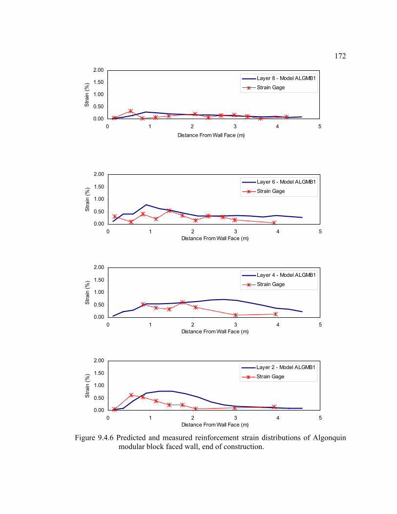
172
Figure 9.4.6 Predicted and measured reinforcement strain distributions of Algonquin modular block faced wall, end of construction.
0.00
0.50
1.00
1.50
2.00
0 1 2 3 4 5Distance From Wall Face (m)
Stra
in (%
)Layer 8 - Model ALGMB1
Strain Gage
0.00
0.50
1.00
1.50
2.00
0 1 2 3 4 5Distance From Wall Face (m)
Stra
in (%
)
Layer 6 - Model ALGMB1
Strain Gage
0.00
0.50
1.00
1.50
2.00
0 1 2 3 4 5Distance From Wall Face (m)
Stra
in (%
)
Layer 4 - Model ALGMB1
Strain Gage
0.00
0.50
1.00
1.50
2.00
0 1 2 3 4 5Distance From Wall Face (m)
Stra
in (%
)
Layer 2 - Model ALGMB1
Strain Gage
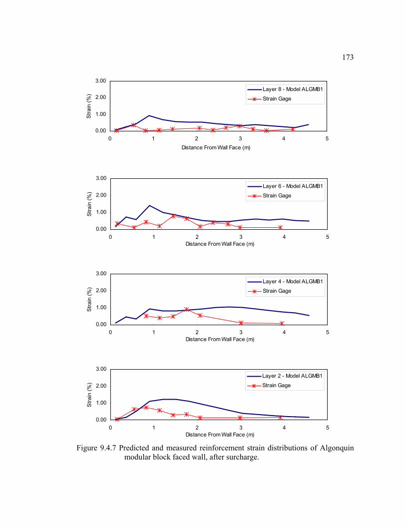
173
Figure 9.4.7 Predicted and measured reinforcement strain distributions of Algonquin modular block faced wall, after surcharge.
0.00
1.00
2.00
3.00
0 1 2 3 4 5Distance From Wall Face (m)
Stra
in (%
)Layer 8 - Model ALGMB1
Strain Gage
0.00
1.00
2.00
3.00
0 1 2 3 4 5Distance From Wall Face (m)
Stra
in (%
)
Layer 6 - Model ALGMB1
Strain Gage
0.00
1.00
2.00
3.00
0 1 2 3 4 5Distance From Wall Face (m)
Stra
in (%
)
Layer 4 - Model ALGMB1
Strain Gage
0.00
1.00
2.00
3.00
0 1 2 3 4 5Distance From Wall Face (m)
Stra
in (%
)
Layer 2 - Model ALGMB1
Strain Gage
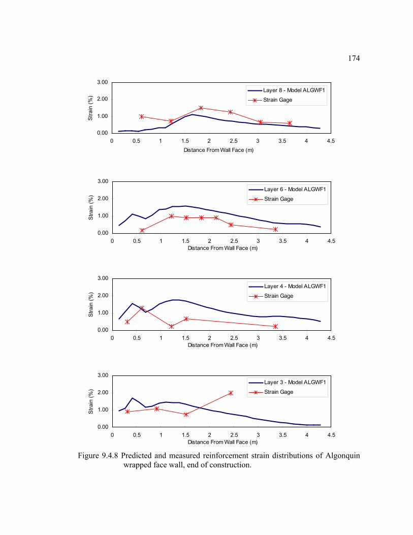
174
Figure 9.4.8 Predicted and measured reinforcement strain distributions of Algonquin wrapped face wall, end of construction.
0.00
1.00
2.00
3.00
0 0.5 1 1.5 2 2.5 3 3.5 4 4.5Distance From Wall Face (m)
Stra
in (%
)Layer 8 - Model ALGWF1
Strain Gage
0.00
1.00
2.00
3.00
0 0.5 1 1.5 2 2.5 3 3.5 4 4.5Distance From Wall Face (m)
Stra
in (%
)
Layer 6 - Model ALGWF1
Strain Gage
0.00
1.00
2.00
3.00
0 0.5 1 1.5 2 2.5 3 3.5 4 4.5Distance From Wall Face (m)
Stra
in (%
)
Layer 4 - Model ALGWF1
Strain Gage
0.00
1.00
2.00
3.00
0 0.5 1 1.5 2 2.5 3 3.5 4 4.5Distance From Wall Face (m)
Stra
in (%
)
Layer 3 - Model ALGWF1
Strain Gage
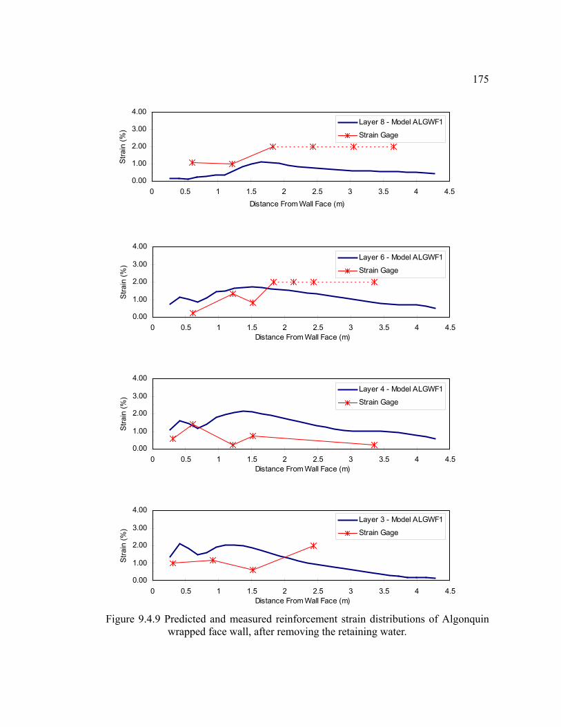
175
Figure 9.4.9 Predicted and measured reinforcement strain distributions of Algonquin wrapped face wall, after removing the retaining water.
0.00
1.00
2.00
3.00
4.00
0 0.5 1 1.5 2 2.5 3 3.5 4 4.5Distance From Wall Face (m)
Stra
in (%
)Layer 8 - Model ALGWF1
Strain Gage
0.00
1.00
2.00
3.00
4.00
0 0.5 1 1.5 2 2.5 3 3.5 4 4.5Distance From Wall Face (m)
Stra
in (%
)
Layer 6 - Model ALGWF1
Strain Gage
0.00
1.00
2.00
3.00
4.00
0 0.5 1 1.5 2 2.5 3 3.5 4 4.5Distance From Wall Face (m)
Stra
in (%
)
Layer 4 - Model ALGWF1
Strain Gage
0.00
1.00
2.00
3.00
4.00
0 0.5 1 1.5 2 2.5 3 3.5 4 4.5Distance From Wall Face (m)
Stra
in (%
)
Layer 3 - Model ALGWF1
Strain Gage

176range at end of construction as well as after removing the retaining water face support.
At end of construction, Model ALGWF1 only under-predicted the reinforcement strain
by 0.5% to 0.8% at the topmost layer (Layer 8). It tended to over-predict the
reinforcement strain by 0.2% to 1.0% at Layers 3, 4, and 6 (Figure 9.4.8). Similar
results were also found after removing the retaining water. Model ALGWF1 tended to
over-predict the reinforcement strains at lower layers (Layers 3 and 4) by an average
of 1.2%, and under-predict the reinforcement strains at Layer 8 (Figure 9.4.9). A
possible reason for the differences between the predicted and measured reinforcement
strains is that the input properties of the nonwoven reinforcement and gabion basket
were determined based on the manufacturer’s information of similar materials. The
actual material properties were not reported in the documentation (Christopher, 1993).
9.4.5 Discussion and Conclusions
1. The developed models were able to reproduce reasonably well in most cases the
reinforcement strain distributions of various GRS walls. The material property
determination procedures and modeling techniques developed in this research were
found to be also suitable for predicting the internal strain levels of various GRS
walls.
2. Accurate material properties were also found to be the key to reproducing the
internal performance data of GRS walls. Results of Model RAING and ALGPC2
showed better predictions of reinforcement strains than the results of Model

177ALGMB1 and ALGWF1 because information about material properties of the
Rainier Avenue wall and Algonquin concrete panel faced wall was more complete.
3. Results of Model ALGMB1 and ALGWF1verified that numerical models
developed using modeling techniques described in Chapter 8 were able to provide
reasonable working strain information of GRS walls, even when insufficient
material information was available and material properties had to be determined
based on information from similar materials.
4. Results of Model ALGWF1 also showed that procedures based on the UCD test
result reported by Boyle (1995) to determine the in-soil stiffness from in-isolation
tests of nonwoven geosynthetics were appropriate. The input stiffness of the
nonwoven geosynthetic reinforcement was determined by multiplying the 2%
strain in-isolation stiffness by five.
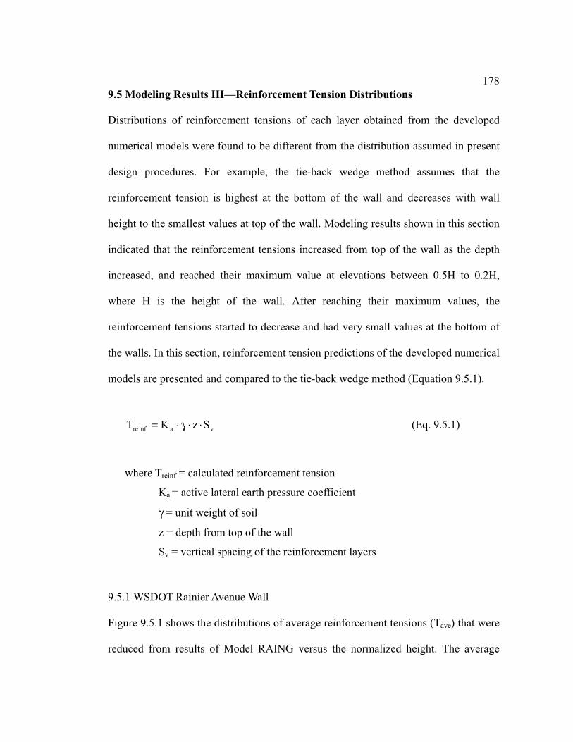
1789.5 Modeling Results III—Reinforcement Tension Distributions
Distributions of reinforcement tensions of each layer obtained from the developed
numerical models were found to be different from the distribution assumed in present
design procedures. For example, the tie-back wedge method assumes that the
reinforcement tension is highest at the bottom of the wall and decreases with wall
height to the smallest values at top of the wall. Modeling results shown in this section
indicated that the reinforcement tensions increased from top of the wall as the depth
increased, and reached their maximum value at elevations between 0.5H to 0.2H,
where H is the height of the wall. After reaching their maximum values, the
reinforcement tensions started to decrease and had very small values at the bottom of
the walls. In this section, reinforcement tension predictions of the developed numerical
models are presented and compared to the tie-back wedge method (Equation 9.5.1).
vainfre SzKT ⋅⋅γ⋅= (Eq. 9.5.1)
where Treinf = calculated reinforcement tension
Ka = active lateral earth pressure coefficient
γ = unit weight of soil
z = depth from top of the wall
Sv = vertical spacing of the reinforcement layers
9.5.1 WSDOT Rainier Avenue Wall
Figure 9.5.1 shows the distributions of average reinforcement tensions (Tave) that were
reduced from results of Model RAING versus the normalized height. The average

179reinforcement tensions (Tave) were determined by multiplying the average predicted
reinforcement strains with the in-soil low strain rate reinforcement stiffness to
represent the overall reinforcement tensions. Modeling results shown in Figure 9.5.1
indicate that the values of Tave increased as the height of the wall decreased at the
upper half of the wall, and they decreased with height of wall at lower half of the wall.
The highest value of Tave appeared at the height equal to 0.25H. Reinforcement
tensions calculated using Equation 9.5.1 were also plotted in Figure 9.5.1 for
comparison. As shown in Figure 9.5.1, the reinforcement tensions calculated by the
tie-back wedge method appear to be much higher than the predicted reinforcement
tensions especially at the lower half of the wall. This observation verifies that the tie-
back method tends to over-design the reinforcement tensions at lower part of the wall.
Possible reasons for this are that the conventional method uses the lateral earth
pressure distribution without modifications for soil-reinforcement interactions and toe
restraint provided by the soil foundation in front of the wall.
9.5.2 Algonquin Concrete Panel Faced Walls
The distribution of reinforcement tension in Model ALGPC2 was also found to be
different than that was assumed in the tie-back method. Figure 9.5.2 shows the
predicted reinforcement tension distribution compared to reinforcement tensions
calculated using Equation 9.5.1. As shown in Figure 9.5.2, the predicted reinforcement
tensions are smaller than the calculated reinforcement tensions, especially at the
bottom of the wall. Model ALGPC2 indicates that the actual maximum reinforcement
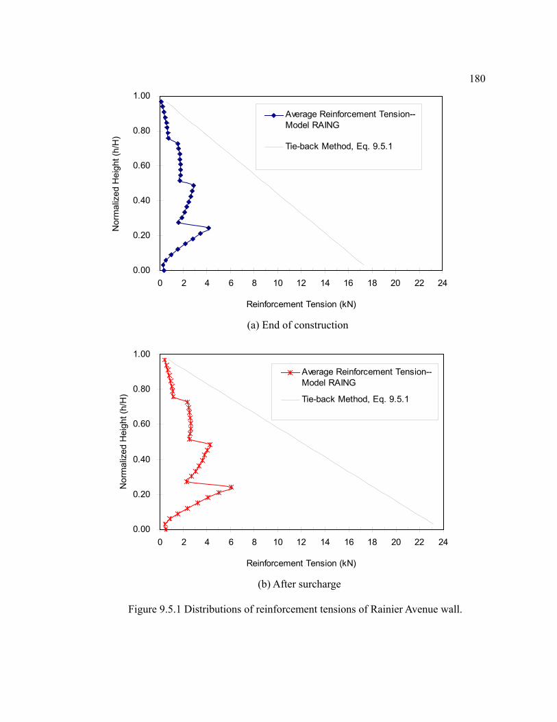
180
(a) End of construction
(b) After surcharge
Figure 9.5.1 Distributions of reinforcement tensions of Rainier Avenue wall.
0.00
0.20
0.40
0.60
0.80
1.00
0 2 4 6 8 10 12 14 16 18 20 22 24
Reinforcement Tension (kN)
Nor
mal
ized
Hei
ght (
h/H
)Average Reinforcement Tension--Model RAING
Tie-back Method, Eq. 9.5.1
0.00
0.20
0.40
0.60
0.80
1.00
0 2 4 6 8 10 12 14 16 18 20 22 24
Reinforcement Tension (kN)
Nor
mal
ized
Hei
ght (
h/H
)
Average Reinforcement Tension--Model RAING
Tie-back Method, Eq. 9.5.1

181
Figure 9.5.2 Distribution of reinforcement tensions of Algonquin concrete panel faced
geogrid wall.
0.0
0.2
0.4
0.6
0.8
1.0
0 2 4 6 8 10 12 14 16 18 20
Reinforcement Tension (kN)
Nor
mal
ized
Hei
ght (
h/H
)
Average Reinforcement Tension--Model ALGPC2
Tie-back Method, Eq. 9.5.1
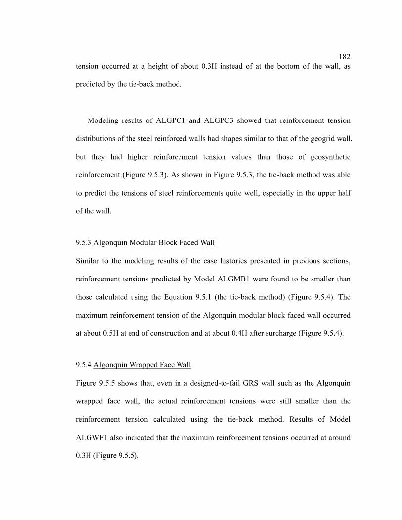
182tension occurred at a height of about 0.3H instead of at the bottom of the wall, as
predicted by the tie-back method.
Modeling results of ALGPC1 and ALGPC3 showed that reinforcement tension
distributions of the steel reinforced walls had shapes similar to that of the geogrid wall,
but they had higher reinforcement tension values than those of geosynthetic
reinforcement (Figure 9.5.3). As shown in Figure 9.5.3, the tie-back method was able
to predict the tensions of steel reinforcements quite well, especially in the upper half
of the wall.
9.5.3 Algonquin Modular Block Faced Wall
Similar to the modeling results of the case histories presented in previous sections,
reinforcement tensions predicted by Model ALGMB1 were found to be smaller than
those calculated using the Equation 9.5.1 (the tie-back method) (Figure 9.5.4). The
maximum reinforcement tension of the Algonquin modular block faced wall occurred
at about 0.5H at end of construction and at about 0.4H after surcharge (Figure 9.5.4).
9.5.4 Algonquin Wrapped Face Wall
Figure 9.5.5 shows that, even in a designed-to-fail GRS wall such as the Algonquin
wrapped face wall, the actual reinforcement tensions were still smaller than the
reinforcement tension calculated using the tie-back method. Results of Model
ALGWF1 also indicated that the maximum reinforcement tensions occurred at around
0.3H (Figure 9.5.5).

183
Figure 9.5.3 Distributions of reinforcement tensions of Algonquin concrete panel
faced walls.
0.0
0.2
0.4
0.6
0.8
1.0
0 2 4 6 8 10 12 14 16 18 20Reinforcement Tension (kN)
Nor
mal
ized
Hei
ght (
h/H
)
Average Reinforcement Tension--Model ALGPC1 (steel)Average Reinforcement Tension--Model ALGPC2 (geosynthetics)Average Reinforcement Tension--Model ALGPC3 (steel)Tie-back Method, Eq. 9.5.1

184
(a) End of construction
(b) After surcharge
Figure 9.5.4 Distributions of reinforcement tensions of Algonquin modular block
faced wall.
0.00
0.20
0.40
0.60
0.80
1.00
0.0 5.0 10.0 15.0 20.0 25.0 30.0 35.0 40.0
Reinforcement Tension (kN/m)
Nor
mal
ized
Hei
ght (
h/H
) Average ReinforcementTension--Model ALGMB1Tie-back Method, Eq. 9.5.1
0.00
0.20
0.40
0.60
0.80
1.00
0.0 5.0 10.0 15.0 20.0 25.0 30.0 35.0 40.0
Reinforcement Tension (kN/m)
Nor
mal
ized
Hei
ght (
h/H
)
Average ReinforcemetnTension-- Model ALGMB1
Tie-back Method, Eq. 9.5.1
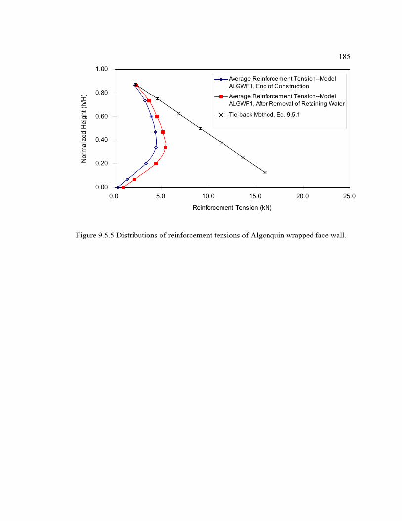
185
Figure 9.5.5 Distributions of reinforcement tensions of Algonquin wrapped face wall.
0.00
0.20
0.40
0.60
0.80
1.00
0.0 5.0 10.0 15.0 20.0 25.0
Reinforcement Tension (kN)
Nor
mal
ized
Hei
ght (
h/H
)Average Reinforcement Tension--ModelALGWF1, End of Construction
Average Reinforcement Tension--ModelALGWF1, After Removal of Retaining Water
Tie-back Method, Eq. 9.5.1
1869.5.5 Discussion and Conclusions
1. Reinforcement tensions calculated using Equation 9.5.1 (the tie-back wedge
method) appeared to be much higher, especially at the lower half of the walls, than
those predicted by the numerical models that were able to reproduce both external
and internal performance of GRS walls. This observation verifies that the
conventional design method tends to over-design the reinforcement tensions in the
lower part of the wall. Possible reasons are that the conventional method uses the
lateral earth pressure distribution without modifications for soil-reinforcement
interactions and toe restraint.
2. Modeling results also showed that actual locations of maximum reinforcement
tensions of GRS walls occurred at heights between 0.2H to 0.5H instead of at
bottom of the walls, as predicted by the tie-back method.

1879.6 Summary and Conclusions
1. Numerical models that were developed using material property determination
procedures described in Chapter 7 and modeling techniques described in Chapter 8
were able to reproduce both external and internal performance of GRS walls
within reasonable ranges.
2. Accurate material properties are concluded as the key to a successful performance
modeling of GRS walls. Results of Models RAING and ALGPC showed better
predictions of wall deflection and reinforcement strain distributions than the
results of Models ALGMB1 and ALGWF1 because information of material
properties of the Rainier Avenue wall and Algonquin concrete panel faced wall
were more complete.
3. For GRS walls with complicated facing systems such as modular block facing,
accurate deflection predictions rely on not only correct input properties of soil and
geosynthetic, but also on the correct input properties of the interfaces between
blocks and reinforcement inserted between the blocks. In Model ALGMB1, input
properties of the interfaces between blocks were determined using the
manufacturer’s information because actual material properties were not reported in
the references. Input properties of reinforcements inserted between blocks can be
determined using connection test data, if available.
4. Modeling results also indicate that soil elements located adjacent to reinforcement
188layers have smaller deformations than soil elements located between the
reinforcements. Especially at the lower half of the GRS walls or at the face of a
wrapped face wall where no structural facing units are used to confine the bulges,
this reinforcing phenomenon becomes more obvious (Figures 9.3.7 and 9.3.8).
5. Differences were found between the modeling results and inclinometer
measurements, especially above the locations of maximum wall deflections
predicted by the numerical models (Figures 9.3.2, 9.3.6, and 9.3.7). The
inclinometer measurements indicated a maximum wall deflection at the top of the
wall, while the modeling results indicated a maximum deflection at about two-
thirds height of the wall. Both predicted and measured results of reinforcement
strain distributions verified that the deflection predictions of the numerical models
and optical face survey are more reasonable than the inclinometer measurements,
i.e. only small deformation occurred at top of the GRS walls. As shown in Figures
9.4.3, 9.4.6 and 9.4.7, both predicted and measured reinforcement strains in the
upper reinforcement layers were smaller than those of the reinforcement layers at
locations where the maximum wall deflections occurred (about two-thirds of the
wall heights).
6. Results of Models ALGMB1 and ALGWF1verified that numerical models
developed using modeling techniques described in Chapter 8 were able to provide
reasonable working strain information of GRS walls when insufficient material
properties were provided and input material properties were determined from

189information on similar materials.
7. Results of Model ALGWF1 also showed that procedures used to determine the in-
soil stiffness from in-isolation test data for nonwoven geosynthetics were
appropriate. The input stiffness of the nonwoven geosynthetic reinforcement was
determined by multiplying the 2% strain in-isolation stiffness by five. This
modification was based on the UCD test result reported by Boyle (1995).
8. Reinforcement tensions calculated using Equation 9.5.1 (the tie-back wedge
method) appeared to be much higher, especially at the lower half of the wall, than
those predicted by the numerical models that were able to reproduce both external
and internal performance of GRS walls. This observation verifies that the
conventional design method tends to over-design the reinforcement tensions,
especially in the lower part of the wall. Possible reasons are that the conventional
method uses a lateral earth pressure distribution without modifications for soil-
reinforcement interactions and toe restraint.
9. Modeling results also showed that actual locations of maximum reinforcement
tensions of GRS walls occurred at heights between 0.2H to 0.5H instead of at
bottom of the walls, as predicted by the tie-back method.

190Chapter 10
Prediction of Performance of Full Scale GRS Test Walls
As a collaborative part of this research, a program to build and test large scale GRS
walls in the laboratory was conducted at the Royal Military College of Canada
(RMCC). The test walls were designed to systematically change design factors such as
reinforcement stiffness and spacing. FLAC models of these test walls were developed
in an attempt to make performance predictions before the walls were constructed (so
called “Class A” predictions). The purposes of this exercise were to:
1. Further examine and improve the developed modeling techniques,
2. Investigate the effects of reinforcement stiffness and reinforcement spacing on
wall performance under high surcharges, and
3. Examine the feasibility of using the developed modeling techniques to perform
parametric analyses of design factors such as reinforcement stiffness and spacing.
In this chapter, a brief description of the RMCC test program as well as the results
of the Class A predictions are presented. Differences between real walls and the
experimental walls tested in laboratory are also discussed.

19110.1 Full Scale GRS Test Walls
The detailed testing program, including material properties, test facility and
instrumentation, and the test results were reported by Burgess (1999). All three RMCC
test walls had the same height (3.6m) and width (3.4m). They were all built on a
concrete laboratory floor. Backfill material was a clean sand with a friction angle
equal to 42 deg and no cohesion. Detailed triaxial and plane strain test results of the
RMC sand were presented in Chapter 7. The reinforcement was a high-density
polypropylene geogrid product (Tensar BX1100). The geogrid reinforcement was
oriented with its machine direction (weak direction) in the plane strain direction of the
test facility to ensure that large wall deflection developed during tests (Burgess, 1999).
Reinforcement stiffness of this geogrid in the machine direction was 110 kN/m at 2%
strain after low strain rate reduction described in Chapter 7. The embedded length of
the reinforcement was 2.5 m.
Commercially available Pisa II blocks manufactured by Unilock Ltd in Georgetown,
Ontario were used as the facing system unit of this study. The blocks were
approximately 300 mm in depth, 150 mm high, 200 mm wide, and had a mass of 20
kg per unit (Burgess, 1999). The interlock between blocks relied on a concrete key on
the top that matched a slot in the bottom of each block, as well as the friction between
the contact surfaces of the blocks. All test walls were fully instrumented, and
performance data were collected during construction and surcharging. Figure 10.1.1
shows the typical cross section of the test walls with instrumentation layout.

192
Figure 10.1.1 Typical cross section of the RMCC test walls with instrumentation layout (after Burgess, 1999).

193
Table 10.1.1 Summary of RMC test walls.
Wall Number
Ultimate Strength of
Reinforcement Tult (kN/m)
Back- Calculated Factor of Safety*
Reinforcement
Spacing, Sv (m)
Maximum Surcharge
Applied, Ps (kPa)
1
12
2.9
0.6
115
2
6**
1.5
0.6
85
3
12
2.0
0.9
95 * Factors of safety is calculated without taking surcharges into consideration. ** The same geogrid used in Wall 1. Reinforcement stiffness and strength were
assumed to be reduced 50% by removing every second longitudinal member of the grid.

194Surcharge was applied on the top of the walls using confined airbags. This method
allowed incremental surcharge control and a relatively high surcharge to be applied.
Table 10.1.1 lists the factor of safety, ultimate strength of the reinforcement, and
maximum surcharge applied to the walls.
10.2 Modeling Result
Three FLAC models were developed to model the performance of test Walls 1, 2, and
3. Model RMC1 was first developed to reproduce the performance of Wall 1. The trial
model of RMC1 failed to predict the performance of Wall 1 because precise
information of the rather complicated boundary conditions, such as the toe restraint,
and the plane strain soil properties were not available at the time of initial prediction.
Model RMC1 was later modified to include improved laboratory boundary conditions,
plane strain soil test results and the low confining pressure dilation angle of the RMC
sand. Although successful prediction was obtained from this improved Model RMC1,
this was not a true Class A prediction because the improved modeling of Wall 1 was
done after the construction and surcharging of Wall 1 were complete.
Models RMC2 and RMC3 were developed based on the improved Model RMC1
and used to perform Class A predictions of test Walls 2 and 3. Both models were able
to predict the performance of test Walls 2 and 3 without any additional modifications.
Because these predictions were made before the instrumentation results become
available, they were true Class A predictions.

195In the following sections, modeling results of Models RMC1, RMC2, and RMC3
are presented and compared with the face deflection measurements and strain gage
measurements of the reinforcement of test Walls 1, 2, and 3.
10.2.1 Wall 1
Figure 10.2.1 shows the predicted and measured wall face deflections at end of
construction. Although Model RMC1 underestimated the face deformation at end of
construction, the maximum difference between the prediction and measurement was
only about 6 mm. The most likely reason for this underestimation is that the numerical
model did not include any additional movements due to the construction procedures
such as backfill compaction. Figure 10.2.2 shows the additional wall deflections after
three surcharge stages (50 kPa, 70 kPa, and 115 kPa) were applied. Results of Model
RMC1 showed a very good agreement to the measurements of wall face deflections.
Model RMC1 was able to predict the maximum face deflections at all different
surcharge stages (only three are shown in Figure 10.2.2 for clarity) and only slightly
overpredicted the deflections at top of the wall. Numerical model tended to
overestimate the wall face deflection at top of the wall after surcharge was applied.
This result could be improved somewhat by decreasing the contact area of the
surcharge pressure. Full contact between airbag and backfill soil was assumed in the
numerical models. During the tests of Walls 1 and 2, a decrease of the surcharge
contact area (area between the airbag and backfill soil) behind the wall face due

196
Figure 10.2.1 Predicted and measured wall face deflection of Wall 1, at the end of construction.
Figure 10.2.2 Additional wall face deflection of Wall 1 after surcharges of 50, 70, and
115 kPa, respectively.
0
0.5
1
1.5
2
2.5
3
3.5
4
0 4 8 12 16 20Face deflection (mm)
Hei
ght o
f the
wal
l (m
)
Predicted- Model RMC1Measured
0
0.5
1
1.5
2
2.5
3
3.5
4
0 20 40 60 80 100 120Face Deflection (mm)
Hei
ght o
f Wal
l (m
)
Predicted- 50kPa
Measured- 50kPa
Predicted- 70kPa
Measured- 70kPa
Predicted- 115kPa
Measured- 115kPa

197to the inflation of the airbag was observed by Burgess (1999). However, the actual
surcharge contact area was not reported by him, so no exact decrease in surcharge
contact area could be modeled. This is probably the reason why the prediction had a
different shape than the measurements and also differed than the modeling results of
case histories shown in Chapter 9.
Figures 10.2.3 to 10.2.6 show the predicted and measured reinforcement strains at
end of construction and for three typical surcharge stages. As shown in Figure 10.2.3b,
results of Model RMC1 shows a good agreement to the strain gage measurements of
reinforcement layers located at upper half of the test wall (Layers 4 to 6). Although
Model RMC1 tended to underestimate the reinforcement strains in lower half of the
wall, the maximum differences between the predictions and the measurements were
less than 0.6%. Figure 10.2.4 shows that, after the 50 kPa surcharge was applied,
Model RMC1 gave very good predictions of reinforcement strains in the upper portion
of the wall (Layer 4 to 6), and still underestimated the reinforcement strains in the
lower portion of the wall by about 1%. Similar observations were also found in the
results of the 70 kPa surcharge stage (Figure 10.2.5). However, as the surcharge
increased, differences between the prediction and measurements also increased. As
shown in Figure 10.2.6, result of RMC1 tended to overpredict the reinforcement strain
in the lower half of the wall by 2 to 3%; yet there still was reasonable agreement to the
strain gage measurements in the upper half of the wall at the last surcharge stage (115
kPa).
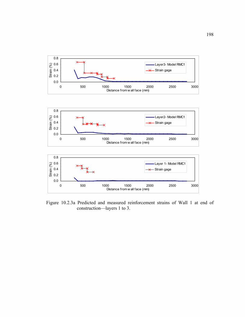
198
Figure 10.2.3a Predicted and measured reinforcement strains of Wall 1 at end of
construction—layers 1 to 3.
0.0
0.2
0.4
0.6
0.8
0 500 1000 1500 2000 2500 3000Distance from w all face (mm)
Stra
in (%
) Layer3- Model RMC1
Strain gage
0.0
0.2
0.4
0.6
0.8
0 500 1000 1500 2000 2500 3000Distance from w all face (mm)
Stra
in (%
) Layer2- Model RMC1
Strain gage
0.0
0.2
0.4
0.6
0.8
0 500 1000 1500 2000 2500 3000Distance from w all face (mm)
Stra
in (%
) Layer 1- Model RMC1
Strain gage

199
Figure 10.2.3b Predicted and measured reinforcement strains of Wall 1 at end of
construction—layers 4 to 6.
-0.1
0.1
0.3
0.5
0.7
0 500 1000 1500 2000 2500 3000Distance from w all face (mm)
Stra
in (%
) Layer6- Model RMC1
Strain gage
0.0
0.2
0.4
0.6
0.8
0 500 1000 1500 2000 2500 3000Distance from w all face (mm)
Stra
in (%
) Layer5- Model RMC1
Strain gage
0.0
0.2
0.4
0.6
0.8
0 500 1000 1500 2000 2500 3000Distance from w all face (mm)
Stra
in (%
) Layer4- Model RMC1
Strain gage

200
Figure 10.2.4a Predicted and measured reinforcement strains of Wall 1 after 50kPa
surcharge—layers 1 to 3.
0.0
2.0
4.0
6.0
0 500 1000 1500 2000 2500 3000Distance from w all face (mm)
Stra
in (%
) Layer3- Model RMC1
Measured
0.0
2.0
4.0
6.0
0 500 1000 1500 2000 2500 3000Distance from w all face (mm)
Stra
in (%
) Layer2- Model RMC1
Measured
0.0
2.0
4.0
6.0
0 500 1000 1500 2000 2500 3000Distance from w all face (mm)
Stra
in (%
) Layer 1- Model RMC1
Measured

201
Figure 10.2.4b Predicted and measured reinforcement strains of Wall 1 after 50kPa
surcharge—layers 4 to 6.
0.0
2.0
4.0
6.0
0 500 1000 1500 2000 2500 3000Distance from w all face (mm)
Stra
in (%
) Layer6- Model RMC1
Measured
0.0
2.0
4.0
6.0
0 500 1000 1500 2000 2500 3000Distance from w all face (mm)
Stra
in (%
) Layer5- Model RMC1
Measured
0.0
2.0
4.0
6.0
0 500 1000 1500 2000 2500 3000Distance from w all face (mm)
Stra
in (%
) Layer4- Model RMC1
Measured

202
Figure 10.2.5a Predicted and measured reinforcement strains of Wall 1 after 70kPa
surcharge—layers 1 to 3.
0.0
2.0
4.0
6.0
8.0
0 500 1000 1500 2000 2500 3000Distance from w all face (mm)
Stra
in (%
) Layer3- Model RMC1
Measured
0.0
2.0
4.0
6.0
8.0
0 500 1000 1500 2000 2500 3000Distance from w all face (mm)
Stra
in (%
) Layer2- Model RMC1
Measured
0.0
2.0
4.0
6.0
8.0
0 500 1000 1500 2000 2500 3000Distance from w all face (mm)
Stra
in (%
) Layer 1- Model RMC1
Measured

203
Figure 10.2.5b Predicted and measured reinforcement strains of Wall 1 after 70kPa
surcharge—layers 4 to 6.
0.0
2.0
4.0
6.0
8.0
0 500 1000 1500 2000 2500 3000Distance from w all face (mm)
Stra
in (%
) Layer6- Model RMC1
Measured
0.0
2.0
4.0
6.0
8.0
0 500 1000 1500 2000 2500 3000Distance from w all face (mm)
Stra
in (%
) Layer5- Model RMC1
Measured
0.0
2.0
4.0
6.0
8.0
0 500 1000 1500 2000 2500 3000Distance from w all face (mm)
Stra
in (%
) Layer4- Model RMC1
Measured

204
Figure 10.2.6a Predicted and measured reinforcement strains of Wall 1 after 115kPa
surcharge—layers 1 to 3.
0.03.06.09.0
12.015.0
0 500 1000 1500 2000 2500 3000Distance from w all face (mm)
Stra
in (%
) Layer3- Model RMC1
Measured
0.03.06.09.0
12.015.0
0 500 1000 1500 2000 2500 3000Distance from w all face (mm)
Stra
in (%
) Layer2- Model RMC1
Measured
0.03.06.09.0
12.015.0
0 500 1000 1500 2000 2500 3000Distance from w all face (mm)
Stra
in (%
) Layer 1- Model RMC1
Measured
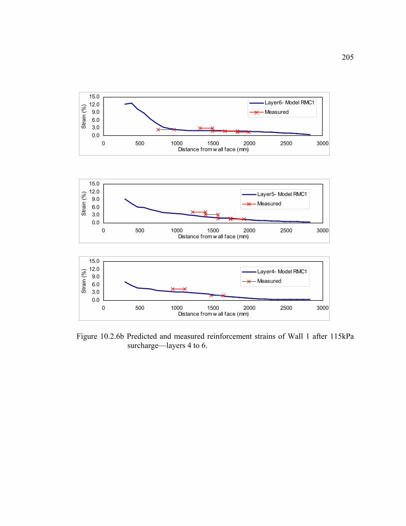
205
Figure 10.2.6b Predicted and measured reinforcement strains of Wall 1 after 115kPa
surcharge—layers 4 to 6.
0.03.06.09.0
12.015.0
0 500 1000 1500 2000 2500 3000Distance from w all face (mm)
Stra
in (%
) Layer6- Model RMC1
Measured
0.03.06.09.0
12.015.0
0 500 1000 1500 2000 2500 3000Distance from w all face (mm)
Stra
in (%
) Layer5- Model RMC1
Measured
0.03.06.09.0
12.015.0
0 500 1000 1500 2000 2500 3000Distance from w all face (mm)
Stra
in (%
) Layer4- Model RMC1
Measured

20610.2.2 Wall 2
Test Wall 2 had the same geometry design and backfill soil as Wall 1; the only
difference between Walls 1 and 2 was the reinforcement stiffness. The reinforcement
stiffness and strength of Wall 2 was decreased by 50% from that of Wall 1 by
eliminating every second longitudinal member of the same geogrid used in Wall 1.
The improved Model RMC1 was modified into Model RMC2 by decreasing the
modulus and yielding strength of the reinforcement to 50% of the value used in Model
RMC1. Different from the analysis performed on Wall 1, true Class A predictions
were performed on test Walls 2 and 3. Performance predictions of these two test walls
were made before the instrumentation became available, and the modeling results
were compared to the instrumentation measurements without any modification. For
Walls 2 and 3, surcharge stages of 30, 40, and 50 kPa were used as the typical
surcharge stages for comparing the predicted and measured wall performance. The
reason for choosing these three surcharge stages is that the input reinforcement
stiffnesses of these test walls were determined at 2% strain, and results of Models
RMC2 and RMC3 indicated that test Walls 2 and 3 developed average strains around
2% at these surcharge stages.
Model RMC2 was able to predict the performance of Wall 2 within a reasonable
range. Figure 10.2.7 shows the wall face deflections at end of construction. As with
Wall 1 Model RMC2 tended to underpredict the maximum deflection, but the
difference was less than 10 mm. After surcharges were applied, Model RMC2 tended

207to overpredicted the measurements by 30 to 40 mm at the locations of maximum
deflections (Figure 10.2.8).
Possible reasons for this overestimation are that the longitudinal member removing
process was assumed to reduce the stiffness of the geogrid by 50%. However, the
actual stiffness of this modified geogrid was not determined (Burgess, 1999), either in-
isolation or when confined by soil. (Performance predictions of Model RMC2 could
be improved by arbitrarily increasing the reinforcement modulus from 50% to 70% of
the original modulus of this geogrid.)
For the internal strain levels of Wall 2, the results of Model RMC2 showed a very
good agreement with the strain gage measurements (Figures 10.2.9 to 10.2.12). As
shown in Figure 10.2.9, Model RMC2 was able to predict the reinforcement strain
distribution of Wall 2 within a reasonable range. Similar to the modeling results of
Model RMC1, Model RMC2 underpredicted the reinforcement strain by less then
0.6% in the lower half of the wall, but had a very good agreement to the measurements
in the upper half of the wall. Figures 10.2.10 and 10.2.11 show the modeling results
compared to the strain gage measurements at two typical surcharge stages of 30 and
40kPa. Model RMC2 gave very good predictions of reinforcement strains in the lower
half of the wall but tended to overpredict them by 1 to 1.5% in the upper half of the
wall. However, modeling results of the surcharge stage of 50kPa had a very good
agreement to the measurements throughout the full wall height (Figure 10.2.12).

208
Figure 10.2.7 Predicted and measured wall face deflection of Wall 2, at the end of
construction.
Figure 10.2.8 Additional wall face deflection of Wall 2 after surcharges of 30, 40, and
50kPa, respectively.
0
0.5
1
1.5
2
2.5
3
3.5
4
0 20 40 60 80 100 120Face Deflection (mm)
Hei
ght o
f Wal
l (m
)
Predicted- 30kPa
Measured- 30kPa
Predicted- 40kPa
Measured- 40kPa
Predicted- 50kPa
Measured- 50kPa
0
0.5
1
1.5
2
2.5
3
3.5
4
0 4 8 12 16 20Face deflection (mm)
Hei
ght o
f the
wal
l (m
)
Predicted- Model RMC2Measured

209
Figure 10.2.9a Predicted and measured reinforcement strains of Wall 2 at end of
construction—layers 1 to 3.
0.0
0.5
1.0
1.5
2.0
0 500 1000 1500 2000 2500 3000Distance from w all face (mm)
Stra
in (%
) Layer3- Model RMC2
Measured
-1.0
-0.5
0.0
0.5
1.0
0 500 1000 1500 2000 2500 3000Distance from w all face (mm)
Stra
in (%
) Layer2- Model RMC1Measured
0.0
0.5
1.0
1.5
2.0
0 500 1000 1500 2000 2500 3000Distance from w all face (mm)
Stra
in (%
) Layer 1- Model RMC2
Measured

210
Figure 10.2.9b Predicted and measured reinforcement strains of Wall 2 at end of
construction—layers 4 to 6.
-0.5
0.0
0.5
1.0
1.5
0 500 1000 1500 2000 2500 3000Distance from w all face (mm)
Stra
in (%
) Layer6- Model RMC2
Measured
-0.5
0.0
0.5
1.0
1.5
0 500 1000 1500 2000 2500 3000Distance from w all face (mm)
Stra
in (%
) Layer5- Model RMC2
Measured
0.0
0.5
1.0
1.5
2.0
0 500 1000 1500 2000 2500 3000Distance from w all face (mm)
Stra
in (%
) Layer4- Model RMC2
Measured

211
Figure 10.2.10a Predicted and measured reinforcement strains of Wall 2 after 30kPa
surcharge—layers 1 to 3.
0.0
2.0
4.0
6.0
8.0
0 500 1000 1500 2000 2500 3000Distance from w all face (mm)
Stra
in (%
) Layer3- Model RMC2
Measured
0.0
2.0
4.0
6.0
8.0
0 500 1000 1500 2000 2500 3000Distance from w all face (mm)
Stra
in (%
) Layer2- Model RMC2
Measured
0.0
2.0
4.0
6.0
8.0
0 500 1000 1500 2000 2500 3000Distance from w all face (mm)
Stra
in (%
) Layer 1- Model RMC2
Measured

212
Figure 10.2.10b Predicted and measured reinforcement strains of Wall 2 after 30kPa
surcharge—layers 4 to 6.
0.0
2.0
4.0
6.0
8.0
0 500 1000 1500 2000 2500 3000Distance from w all face (mm)
Stra
in (%
) Layer6- Model RMC2
Measured
0.0
2.0
4.0
6.0
8.0
0 500 1000 1500 2000 2500 3000Distance from w all face (mm)
Stra
in (%
) Layer5- Model RMC2
Measured
0.0
2.0
4.0
6.0
8.0
0 500 1000 1500 2000 2500 3000Distance from w all face (mm)
Stra
in (%
) Layer4- Model RMC2
Measured

213
Figure 10.2.11a Predicted and measured reinforcement strains of Wall 2 after 40kPa
surcharge—layers 1 to 3.
0.02.04.06.08.0
10.0
0 500 1000 1500 2000 2500 3000Distance from w all face (mm)
Stra
in (%
) Layer3- Model RMC2
Measured
0.02.04.06.08.0
10.0
0 500 1000 1500 2000 2500 3000Distance from w all face (mm)
Stra
in (%
) Layer2- Model RMC2
Measured
0.02.04.06.08.0
10.0
0 500 1000 1500 2000 2500 3000Distance from w all face (mm)
Stra
in (%
) Layer 1- Model RMC2
Measured
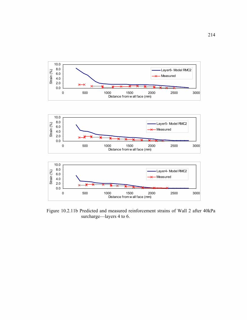
214
Figure 10.2.11b Predicted and measured reinforcement strains of Wall 2 after 40kPa
surcharge—layers 4 to 6.
0.02.04.06.08.0
10.0
0 500 1000 1500 2000 2500 3000Distance from w all face (mm)
Stra
in (%
) Layer6- Model RMC2
Measured
0.02.04.06.08.0
10.0
0 500 1000 1500 2000 2500 3000Distance from w all face (mm)
Stra
in (%
) Layer5- Model RMC2
Measured
0.02.04.06.08.0
10.0
0 500 1000 1500 2000 2500 3000Distance from w all face (mm)
Stra
in (%
) Layer4- Model RMC2
Measured

215
Figure 10.2.12a Predicted and measured reinforcement strains of Wall 2 after 50kPa
surcharge—layers 1 to 3.
0.02.04.06.08.0
10.0
0 500 1000 1500 2000 2500 3000Distance from w all face (mm)
Stra
in (%
) Layer3- Model RMC2
Measured
0.02.04.06.08.0
10.0
0 500 1000 1500 2000 2500 3000Distance from w all face (mm)
Stra
in (%
) Layer2- Model RMC2
Measured
0.02.04.06.08.0
10.0
0 500 1000 1500 2000 2500 3000Distance from w all face (mm)
Stra
in (%
) Layer 1- Model RMC2
Measured

216
Figure 10.2.12b Predicted and measured reinforcement strains of Wall 2 after 50kPa
surcharge—layers 4 to 6.
0.02.04.06.08.0
10.0
0 500 1000 1500 2000 2500 3000Distance from w all face (mm)
Stra
in (%
) Layer6- Model RMC2
Measured
0.02.04.06.08.0
10.0
0 500 1000 1500 2000 2500 3000Distance from w all face (mm)
Stra
in (%
) Layer5- Model RMC2
Measured
0.02.04.06.08.0
10.0
0 500 1000 1500 2000 2500 3000Distance from w all face (mm)
Stra
in (%
) Layer4- Model RMC2
Measured
217
10.2.3 Wall 3
Test Wall 3 was designed using the same backfill and reinforcement materials as Wall
1. However, in Wall 3, the reinforcement spacing was increased to 0.9 m, or 50%
more than the reinforcement spacing used in Walls 1 and 2 (Table 10.1.1). Model
RMC3 was developed by increasing the reinforcement spacing of Model RMC1.
Performance prediction of Wall 3 was made using Model RMC3 before the
instrumentation measurements became available, another true Class A prediction.
However, unfortunately, wall deflection and reinforcement strain data was not fully
reduced when this disseration was in preparation. Modeling results were only
compared to the raw data of the wall face deflection survey at the end of construction
and raw strain gage measurements.
However, results of Model RMC3 indicated that a successful Class A prediction
was achieved. Figure 10.2.13 shows the predicted and measured wall face deflections
at end of construction. Model RMC3 underpredicted the maximum face deflection by
only 6 mm. Reduced face deflection measurements after surcharges were not available
at the time when this dissertation was in preparation.
Figures 10.2.14 to 10.2.17 show that Model RMC3 made reasonable predictions of
the reinforcement strains. At the end of construction stage, Model RMC3
underpredicted the reinforcement strains by 0.2 to 0.6% in the lower half of the wall
and by less than 0.3% in the upper half of the wall (Figure 10.2.14). For three typical
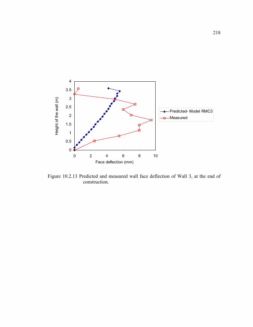
218
Figure 10.2.13 Predicted and measured wall face deflection of Wall 3, at the end of
construction.
0
0.5
1
1.5
2
2.5
3
3.5
4
0 2 4 6 8 10Face deflection (mm)
Hei
ght o
f the
wal
l (m
)
Predicted- Model RMC3Measured
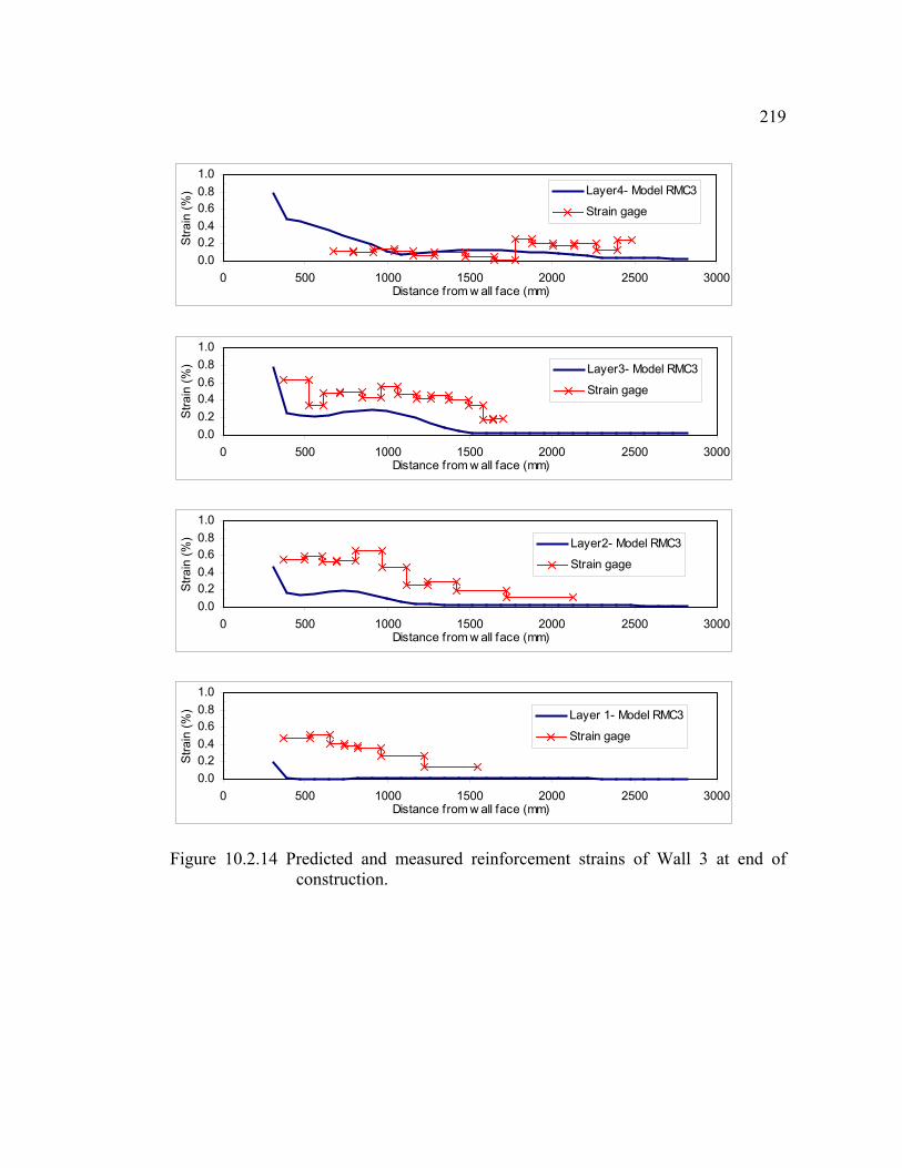
219
Figure 10.2.14 Predicted and measured reinforcement strains of Wall 3 at end of
construction.
0.00.20.40.60.81.0
0 500 1000 1500 2000 2500 3000Distance from w all face (mm)
Stra
in (%
) Layer4- Model RMC3
Strain gage
0.00.20.40.60.81.0
0 500 1000 1500 2000 2500 3000Distance from w all face (mm)
Stra
in (%
) Layer3- Model RMC3
Strain gage
0.00.20.40.60.81.0
0 500 1000 1500 2000 2500 3000Distance from w all face (mm)
Stra
in (%
) Layer2- Model RMC3
Strain gage
0.00.20.40.60.81.0
0 500 1000 1500 2000 2500 3000Distance from w all face (mm)
Stra
in (%
) Layer 1- Model RMC3
Strain gage

220
Figure 10.2.15 Predicted and measured reinforcement strains of Wall 3 after 30kPa
surcharge.
0.0
1.0
2.0
3.0
4.0
0 500 1000 1500 2000 2500 3000Distance from w all face (mm)
Stra
in (%
) Layer4- Model RMC3
Measured
0.0
1.0
2.0
3.0
4.0
0 500 1000 1500 2000 2500 3000Distance from w all face (mm)
Stra
in (%
) Layer3- Model RMC3
Measured
0.0
1.0
2.0
3.0
4.0
0 500 1000 1500 2000 2500 3000Distance from w all face (mm)
Stra
in (%
) Layer2- Model RMC3
Measured
0.0
1.0
2.0
3.0
4.0
0 500 1000 1500 2000 2500 3000Distance from w all face (mm)
Stra
in (%
) Layer 1- Model RMC3
Measured

221
Figure 10.2.16 Predicted and measured reinforcement strains of Wall 3 after 40kPa
surcharge.
0.0
2.0
4.0
6.0
0 500 1000 1500 2000 2500 3000Distance from w all face (mm)
Stra
in (%
) Layer4- Model RMC3
Measured
0.0
2.0
4.0
6.0
0 500 1000 1500 2000 2500 3000Distance from w all face (mm)
Stra
in (%
) Layer3- Model RMC3
Measured
0.0
2.0
4.0
6.0
0 500 1000 1500 2000 2500 3000Distance from w all face (mm)
Stra
in (%
) Layer2- Model RMC3
Measured
0.0
2.0
4.0
6.0
0 500 1000 1500 2000 2500 3000Distance from w all face (mm)
Stra
in (%
) Layer 1- Model RMC3
Measured

222
Figure 10.2.17 Predicted and measured reinforcement strains of Wall 3 after 50kPa
surcharge.
0.0
2.0
4.0
6.0
8.0
0 500 1000 1500 2000 2500 3000Distance from w all face (mm)
Stra
in (%
) Layer4- Model RMC3
Measured
0.0
2.0
4.0
6.0
8.0
0 500 1000 1500 2000 2500 3000Distance from w all face (mm)
Stra
in (%
) Layer3- Model RMC3
Measured
0.0
2.0
4.0
6.0
8.0
0 500 1000 1500 2000 2500 3000Distance from w all face (mm)
Stra
in (%
) Layer2- Model RMC3
Measured
0.0
2.0
4.0
6.0
8.0
0 500 1000 1500 2000 2500 3000Distance from w all face (mm)
Stra
in (%
) Layer 1- Model RMC3
Measured
223
surcharge stages (30 kPa, 40 kPa, and 50 kPa), Model RMC3 was able to predict the
reinforcement strain distributions of Wall 3 quite well (Figures 10.2.15 to 10.2.17). It
tended to underpredict the reinforcement strains only at Layer 1 by 0.5 to 1% for the
30kPa surcharge stage, and had very good strain predictions for the other three
reinforcement layers (Figure 10.2.15). For the 40 kPa and 50 kPa surcharge stages,
Model RMC3 was able to predict quite well the reinforcement strains of all layers
(Figures 10.2.16 and 10.2.17).
10.3 Difference Between Test Walls and Real Walls
The RMCC test walls were built in the laboratory in order to have better control of the
materials, instrumentation, and construction. However, when utilizing information
obtained from the test wall to extrapolate to the behavior of real walls, as well as to
calibrate numerical models, following differences between test walls and real walls
have to be considered:
1. The toes of the test walls were restrained by hydraulic jacks in order to measure
the reaction forces at the toe under the modular blocks (Figure 10.2.1). The
hydraulic jacks were then released after last surcharge stage was reached. This
type of toe restraint was very different from those of real walls. It was also very
difficult to be accurately simulated in FLAC.

224
2. Surcharge of the test wall was applied using airbags. This is different from the
surcharge applied by real soil in that the contact area at the edge between the
airbag and the backfill decreased as the airbag inflated.
3. The RMCC test walls were built on a very stiff concrete foundation surrounded by
three reinforced concrete reaction walls. Movements of the backfill soil were
confined at the bottom of the wall. Therefore, the deformation and stress
distributions at the bottom of the test walls, especially at the area around the toe of
the wall, are very different from those of real walls built on soil foundations.
Comparison of the performance of the in-laboratory test wall (Wall 1) and the test
wall built in the field (Algonquin modular block wall) are presented and discussed in
the following section.
10.4 Discussions and Conclusions
1. Numerical models tended to underpredict the wall face deflection at end of the
construction by only about 6 to 10mm. The most likely reason for this
underestimation is that the additional movement due to the construction
procedures such as soil compaction was not considered in the FLAC models.
2. Numerical models tended to overestimate the wall face deflection at top of the wall
after surcharge was applied. This result could be improved somewhat by

225
decreasing the contact area of the surcharge pressure. Full contact between airbag
and backfill soil was assumed in the numerical models. During the tests of Walls 1
and 2, a decrease of the surcharge contact area (area between the airbag and
backfill soil) behind the wall face due to the inflation of the airbag was observed
by Burgess (1999). However, the actual surcharge contact area was not reported by
him, so no exact decrease in surcharge contact area could be modeled.
3. Overall, the FLAC models tended to underpredict the reinforcement strains in the
lower half of the test walls. A possible reason of this underestimation is that the
FLAC models did not model the toe restraint of the test wall very well.
4. By comparing the results of RMC1, RMC2, and RMC3, improved predictions of
Wall 1 and Wall 3 were made. Test wall Wall 2 was constructed using the same
geogrids as that of Walls 1 and 3 but with every second longitudinal member of
the grid removed. This process was assumed to reduce the stiffness of the geogrid
by 50%. However, the actual stiffness reduction of this modified geogrid was not
measured, and no possible modification in stiffness when the geogrid was confined
by soil was considered. Performance predictions of Model RMC2 could be
improved by increasing the reinforcement modulus from 50% to 70% of the
original modulus of this geogrid.

226
5. Both numerical models and post-construction observations of the test walls
indicated that large differential settlements occurred between the facing blocks and
the backfill soil. However, the strain gage measurements did not show any strain
peaks near the blocks.
6. The stiff concrete foundation of the test walls did affect both the face deflection
profile and the reinforcement tension distribution, as shown in the normalized
plots of Figures 10.4.1 and 10.4.2. Figures 10.4.1 and 10.4.2 show the results of
RMCC Wall 1 compared to the FHWA Algonquin modular block faced wall that
was described in Chapter 9. Figure 10.4.1 indicates that the maximum face
deflection of the wall with a stiff concrete foundation is located at top of the wall,
while that of the wall with a soil foundation is located near the middle of the wall.
Figure 10.4.2 also indicates that a stiff foundation has a similar effect on the
reinforcement tension distributions. The maximum reinforcement tension of the
test wall with a stiff concrete foundation occurred at a height of 0.8H, but the
maximum reinforcement tension of the test wall with a soil foundation occurred at
a height of 0.5H.
It should be emphasized that performance predictions presented in this chapter are
Class A prediction results, i.e. these modeling results were made before the
construction of these test walls. Refinement is always possible after prediction. For
example, face deflection predictions after surcharge can be further improved by

227
Figure 10.4.1 Normalized face deflections for GRS test walls with different foundations.
Figure 10.4.2 Normalized maximum reinforcement tension distributions for GRS test walls with different foundations.
0
0.2
0.4
0.6
0.8
1
1.2
0 0.2 0.4 0.6 0.8 1 1.2
Normalized Wall Face Deflection (d/dmax)
Nor
mal
ized
Hei
ght (
h/H
) Algonquin modular blockfaced wall--soil foundation
RMCC test wall--stifffoundation
0
0.2
0.4
0.6
0.8
1
0 0.2 0.4 0.6 0.8 1 1.2
Normalized Maximum Reinforcement Tension (T/Tmax)
Nor
mal
ized
Hei
ght (
h/H
)
Algonquin modular blockfaced wall--soil foundationRMCC test wall--stifffoundation

228
decreasing the contact area of the surcharge. Moreover, performance simulation of test
Wall 2 can be improved by increasing the reinforcement modulus from 50% to 70% of
the original modulus of the geogrid used in test Walls 1 and 3.
229
Chapter 11
Analytical Models of Lateral Reinforced Earth Pressure and
Composite Modulus of Geosynthetic Reinforced Soil
Two important design factors in present GRS wall design procedures are the
distribution of lateral earth pressure and the reinforcement stiffness. These two factors
are determined based on properties of the individual construction materials of the GRS
wall. Present designs requires an assumption of the lateral earth pressure distribution,
and the in-isolation stiffness of geosynthetic reinforcement is usually used. Available
evidence from full-scale and model GRS walls indicates that present design
procedures tend to significantly overestimate the internal lateral stress distribution
within the structure (Bell et al., 1983; Allen et al., 1992; Rowe and Ho, 1993;
Christopher, 1993). Modeling results presented in Chapter 9 of this thesis also suggest
that the soil-only coefficients of lateral earth pressure and in-isolation stiffness of
geosynthetics are not appropriate for characterizing the working stress or strain
distribution inside GRS walls.
In order to analyze the composite GRS behavior, two new terms, the coefficient of
lateral reinforced earth pressure, Kcomp, and composite modulus of geosynthetic
reinforced soil, Ecomp, are introduced in this research. In this chapter, the analytical
models, derivations, and applications of both Kcomp and Ecomp are presented.
Information on the working stress and strain obtained from the results of parametric

230study that are presented in Chapter 12 are characterized using these two GRS
composite terms.
11.1 Lateral Reinforced Earth Pressure
An important internal design consideration of GRS retaining structures is the lateral
earth pressure distribution behind the face of the wall. However, none of the lateral
earth pressure distributions used in present GRS wall design procedures have clearly
taken the reinforcing effects contributed by reinforcement into account. An alternate
approach to obtain the distribution of lateral reinforced earth pressure behind the wall
face was developed in this research (Lee, 1999). This alternate approach combines the
conventional lateral earth theory (Rankine earth pressure theory) and reinforcement
tension using free body diagrams.
11.1.1 Analytical Model of Lateral Reinforced Earth Pressure
Figure 11.1.1 shows the lateral earth pressure distribution behind the face of a
conventional unreinforced retaining wall. In Figure 11.1.1, Fsoil represents the total
earth force supported by the facing blocks. H and Hs are height of the wall and
location of the Fsoil, respectively. Equation 11.1.1 is the general mathematical
expression of the lateral earth pressure distribution for this case.

231
zKpsoil ⋅γ⋅=
Figure 11.1.1 Lateral earth pressure distribution of an unreinforced retaining wall.
Fsoil
z
Hs
H

232
zKpsoil ⋅γ⋅= (Eq. 11.1.1)
where K = lateral earth pressure coefficient,
γ = unit weight of soil, and
z = depth from top of the wall.
When planar reinforcements such as geosynthetics are inserted into the wall
backfill, the lateral earth pressure distribution is changed because of the presence of
the reinforcement tensions, as shown schematically in Figure 11.1.2. In Figure 11.1.2,
Ftotal represents the total force of the GRS retaining structure supported by the facing
system, and H1 is the location of Ftotal. tn is the reinforcement tension per unit width at
reinforcement layer n.
The lateral GRS composite distribution can be determined by superposing the
lateral earth pressure and the reinforcement tensions behind the wall face (Figure
11.1.3). In order to characterize the lateral earth pressure distribution of the GRS
composite, a new lateral pressure coefficient, Kcomp, is defined as the composite lateral
earth pressure coefficient of the geosynthetic reinforced soil.

233
t1
t2
tn
Ftotal
z
H1
H
zKpsoil ⋅γ⋅=
Figure 11.1.2. Lateral earth pressure distribution in a geosynthetic reinforced retaining wall.

234
HFtotal
H1
z
zKp compcomp ⋅γ⋅=
Figure 11.1.3 Lateral composite pressure distribution of a reinforced retaining wall.

235The mathematical expression of Kcomp at any depth from the top of the backfill can
be derived by comparing Figures 11.1.2 and 11.1.3 (Equation 11.1.2).
Ftotal (z) = Fsoil (z) - ∑=
n
1iit (Eq. 11.1.2)
where Ftotal (z) = total force supported by the facing at depth z,
Fsoil (z) = Total earth force supported by the facing at depth z, and
∑=
n
1iit = Total tensile forces of reinforcement at depth z.
By introducing the integral forms of the Ftotal and Fsoil, Equation 11.1.2 can be re-
written as Equation 11.1.3.
∑∫∫=
−==n
1ii
z
0soil
z
0comptotal tdA)z(pdA)z(p)z(F (Eq. 11.1.3)
By assuming that the retaining wall has width equal to unity (dA = dz) and
performing the integration with definitions of the lateral earth pressure distributions as
shown in Figures 11.1.1, 11.1.2, and 11.1.3, Equation 11.1.3 can be reduced to
Equation 11.1.4.
∑=
−⋅γ⋅=⋅γ⋅=n
1ii
2
soil
2
comptotal t2zK
2zK)z(F (Eq. 11.1.4)

236The mathematical expression of the composite lateral earth pressure coefficient at
any depth can then be obtained by rearranging Equation 11.1.4 (Equation 11.1.5).
2
n
1ii
soilcomp z
t2K)z(K
⋅γ
⋅−=
∑= (Eq. 11.1.5)
Reinforcement tensions needed to stabilize the backfill soil at depth z can also be
obtained by rearranging Equation 11.1.4 (Equation 11.1.6).
)KK(2z)z(t compsoil
2n
1i −⋅⋅γ=∑ (Eq. 11.1.6)
11.1.2 Value of Kcomp
Direct measurements of the lateral earth pressures behind the face of the GRS
retaining walls are not available today because accurate field measurements of earth
pressures are virtually impossible to obtain. It is also difficult to determine Kcomp using
Equation 11.1.5 because the state of the backfill soil (Ksoil), whether active, at rest, or
passive, is hard to determine. However, reliable prediction of the GRS composite
lateral earth pressures can be obtained from well-developed numerical models that are
capable of reproducing the internal strain measurements within a GRS wall using
Equation 11.1.7, provided that the in-soil modulus of the reinforcement is known. In
Equation 11.1.7, modeling results of horizontal stresses of soil elements behind the

237
wall faces were used as the horizontal geosynthetic reinforced earth pressure, σh, in the
equation.
z)z(K h
comp ⋅γσ
= (Eq. 11.1.7)
where σh = horizontal geosynthetic reinforced earth pressure obtained from
numerical models.
Modeling results of the WSDOT Rainier Avenue wall, the FHWA Algonquin concrete
panel geogrid wall, and the FHWA Algonquin modular block faced wall were reduced
to obtain typical values of Kcomp for different types of GRS walls. Figures 11.1.4 to
11.1.6 show the values of Kcomp that were obtained from modeling results, as well as
the active lateral earth pressure coefficient, Ka, and the lateral earth pressure
coefficient at rest, Ko. Values of Kcomp shown in Figures 11.1.4 to 11.1.6 were
determined using Equation 11.1.7. Table 11.1.1 summarizes the typical values of
coefficient of lateral reinforced earth pressure, Kcomp, Ka, and Ko.
11.1.3 Discussion and Conclusions
1. Equation 11.1.5 shows that the GRS composite lateral earth pressure distribution is
a function of the height of the wall, unit weight and the lateral earth pressure
coefficient of the backfill soil, and the distribution of the reinforcement tension.
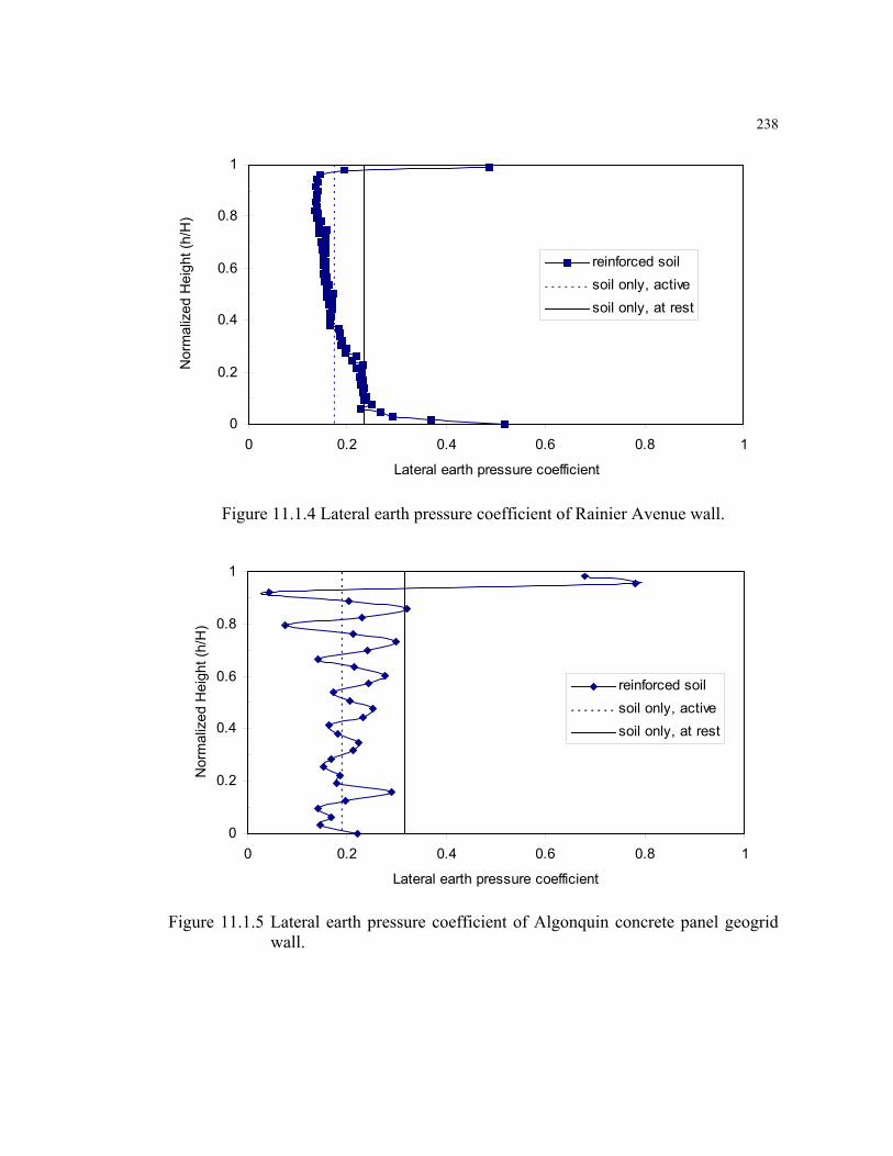
238
Figure 11.1.4 Lateral earth pressure coefficient of Rainier Avenue wall.
Figure 11.1.5 Lateral earth pressure coefficient of Algonquin concrete panel geogrid wall.
0
0.2
0.4
0.6
0.8
1
0 0.2 0.4 0.6 0.8 1
Lateral earth pressure coefficient
Nor
mal
ized
Hei
ght (
h/H
)
reinforced soilsoil only, activesoil only, at rest
0
0.2
0.4
0.6
0.8
1
0 0.2 0.4 0.6 0.8 1
Lateral earth pressure coefficient
Nor
mal
ized
Hei
ght (
h/H
)
reinforced soilsoil only, activesoil only, at rest

239
Figure 11.1.6 Lateral earth pressure coefficient of Algonquin modular block faced wall.
Table 11.1.1 Lateral earth pressure coefficients of GRS walls.
Wall Names Kcomp1 Ka
2 K03
Rainier Avenue wall 0.178 0.172 0.234
Algonquin concrete panel geogrid wall
0.20
0.19
0.318
Algonquin modular block faced wall
0.174
0.214
0.318
1 Average of values shown in Figures 11.1.4 to 11.1.6. 2 calculated using Coulomb's equation. 3 1 - sinφ.
0
0.2
0.4
0.6
0.8
1
0 0.2 0.4 0.6 0.8 1
Lateral earth pressure coefficient
Nor
mal
ized
Hei
ght (
h/H
)
reinforced soilsoil only, activesoil only, at rest

240
2. Equation 11.1.5 also indicates that the lateral geosynthetic reinforced earth
pressures behind the wall face can be less than the active lateral earth pressures
when the backfill reaches its active state and the reinforcement starts to provide
tensile forces that reinforce the backfill. Result shown in Figure 11.1.6 and most of
the heights of Figures 11.1.4 and 11.1.5 confirms this observation.
11.2 GRS Composite Modulus, Ecomp
Another term that was developed in this research is the GRS composite modulus
Ecomp. Ecomp was developed based on the theory of composite materials. It was used to
characterize the modeling results of the parametric study described in Chapter 12.
Horizontal face deflections of GRS walls of different designs were found to have a
very good correlation with Ecomp. In the following sections, derivation of Ecomp is
presented. Applications of Ecomp are presented in both Chapters 12 and 14.
Figure 11.2.1 shows a typical cross section of a GRS wall and a GRS element cut
from it. Following assumptions were made in order to simplify the derivations:
1. Deformation of the GRS element is uniform, i.e., there is no interlayer
movement between soil and reinforcement.
2. Width of GRS element equals unity.
3. Stress-strain behavior of the soil and reinforcement follows Hooke’s Law
( ε⋅=σ E ).

241
Figure 11.2.1 GRS element inside a GRS wall.
Soil
Geosynthetic Reinforcement
ts
tg
Sv Fs
Fg
εt= εg= εs

24211.2.1 Derivation of Ecomp
As shown in Figure 11.2.1, the total horizontal force acting on the GRS element can
be expressed as Equation 11.2.1.
sgt FFF += (Eq. 11.2.1)
where Ft = total force of GRS composite,
Fg = reinforcement force, and
Fs = soil force.
Equation 11.2.1 can also be expressed in term of stresses and areas (Equation
11.2.2).
ssggtt AAA ⋅σ+⋅σ=⋅σ (Eq. 11.2.2)
where σt= total stress in the GRS composite,
At= total cross section area of GRS composite,
σg= reinforcement stress,
Ag= cross section area of reinforcement,
σs= soil stress, and
As= cross section area of soil.
Equation 11.2.2 can be further simplified by introducing the assumption that the
width of the wall is equal to unity (Equation 11.2.3).

243
ssggvt ttS ⋅σ+⋅σ=⋅σ (Eq. 11.2.3)
where Sv = height of the GRS composite (reinforcement spacing),
tg = thickness of reinforcement, and
ts = thickness of soil.
Equation 11.2.3 can be rewritten as Equation 11.2.4 using the stress-strain
relationship described by Hooke’s Law ( iii E ε⋅=σ ).
sssgggvtcomp tEtESE ⋅ε⋅+⋅ε⋅=⋅ε⋅ (Eq. 11.2.4)
where Ecomp= modulus of GRS composite,
εt= total strain of GRS composite,
Eg= modulus of reinforcement,
εg= strain of reinforcement,
Es= modulus of soil, and
εs= strain of soil.
Strains εt, εg, and εs in Equation 11.2.4 can be cancelled out because uniform
deformation was assumed (Equation 11.2.5).
ssggvcomp tEtESE ⋅+⋅=⋅ (Eq. 11.2.5)

244Rearranging Equation 11.2.5 and with the relation between tg, ts, and Sv as shown
in Figure 11.2.1, Ecomp can be obtained as Equation 11.2.6:
v
gvs
v
ggcomp S
)tS(E
St
EE−
⋅+⋅= (Eq. 11.2.6)
where vgv StS ≈− , and
gg t
JE = , where J is the stiffness of the reinforcement.
Formulation of Ecomp then becomes:
svv
vs
v
g
gcomp E
SJ
SS
ESt
tJE +=⋅+⋅≈ (Eq. 11.2.7)
11.2.2 Discussion and Conclusions
1. Equation 11.2.7 is the expression for horizontal modulus of the GRS composite.
Derivation of vertical composite modulus of GRS element is different. Moduli
calculated using Equation 11.2.7 are only appropriate for characterizing the
horizontal working stress or strain information of GRS walls.

2452. The in-soil and low strain rate adjustments discussed in Chapter 7 of this thesis
have to be applied to the in-isolation reinforcement stiffness before it is used in
Equation 11.2.7.
3. Plane strain soil modulus is suggested for use in Equation 11.2.7 when analyzing
GRS retaining structures. Es, the soil modulus, can be obtained from strength test
data or estimated using a confining pressure dependent hyperbolic soil modulus
model. Details of estimating plane strain soil modulus are described in Chapter 7
of this thesis as well.
246Chapter 12
Parametric Study of the Internal Design Factors of GRS Walls
12.1 Introduction
After the successful performance predictions of case histories and large-scale test
walls, extensive parametric studies were performed to investigate the influence of
internal design factors such as layer spacing, soil strength properties, reinforcement
stiffness, and facing types. The results of the parametric analyses were recorded and
analyzed in terms of GRS wall performance factors such as internal stress-strain levels
and wall face deflections. The purposes of the parametric study were to:
1. Investigate the sensitivity of the modeling results to the input material properties,
2. Examine the influence of the internal design factors on the performance of GRS
retaining structures, and
3. Make attempts to improve the internal design of GRS walls based on the working
stress information obtained from the parametric study.
Two types of parametric analyses were performed in this research. In the first type,
numerical models of the WSDOT Rainier Avenue wall (Model 5008P) and the FHWA
Algonquin concrete panel test walls (Models AlgW1, AlgW2, and AlgW3) were used
as the fundamental models of the parametric study. Internal design factors such as soil
friction angle and reinforcement stiffness were systematically varied in the models.
These analyses were performed by varying only one design factor in each group while

247the other factors were fixed. The second type of parametric study was performed using
a large number of GRS wall models with different internal stability design factors.
Design factors such as wall height, layer spacing, soil strength properties, and
reinforcement properties were systematically introduced into GRS wall models to
observe the interaction effects of these design factors. In this chapter, results of the
parametric study are presented and discussed.
12.2 Preliminary Parametric Study I -- Rainier Avenue Wall
The first parametric study was performed on Model 5008P to examine its sensitivity to
the input material properties. Maximum face deflections of the model walls were
examined by systematically varying the input material properties such as the
reinforcement stiffness, the soil friction angle, and the soil cohesion. Table 12.2.1 lists
the values of the material properties that were input into Model 5008P. Only one
design factor (input material property) was changed in each group while the other
factors were fixed.
The results of this parametric analysis have already been presented by Holtz and
Lee (1997). Figures 12.2.1 to 12.2.3 show the results of this preliminary study. The
maximum deflections increased when the tensile modulus of geosynthetics decreased
(Figure 12.2.1). The same tendency was also observed in Figure 12.2.2; the maximum
deflection increased when the soil friction angle decreased. Although the maximum
deflections decreased slightly when the soil cohesion was decreased from 8 kPa to 6
kPa, they increased as the soil cohesion decreased further (Figure12.2.3).

248
Table 12.2.1 Input material properties used in parametric study.
Input material properties Values
Reinforcement stiffness 12.5%, 25%, 50%, and 75% of the original reinforcement stiffnesses
(Table 9.2.1) Soil friction angle 30, 35, 40, 45, 50, and 55 degrees
Soil cohesion 0, 2, 4, 6, and 8kPa
Figure 12.2.1 Maximum deflection vs. geosynthetic modulus.
0
0.2
0.4
0.6
0.8
1
1.2
0 100 200 300 400 500 600 700 800 900
Maximum Deflection (mm)
(Geo
synt
hetic
Mod
ulus
) / (O
rigin
alG
eosy
nthe
tic M
odul
us) Maximum Deflection, Wall
FaceMaximum Delfection, 2.7mbehind Wall Face

249
Figure 12.2.2 Maximum deflection vs. soil friction angle.
Figure 12.2.3 Maximum deflection vs. soil cohesion
20
25
30
35
40
45
50
55
60
0 50 100 150 200 250 300 350
Maximum Deflection (mm)
Fric
tion
Angl
e (d
eg.)
Maximum Deflection, WallFaceMaximum Delfection, 2.7mbehind Wall Face
0
1
2
3
4
5
6
7
8
9
0 20 40 60 80 100 120 140 160 180 200
Maximum Deflection (mm)
Coh
esio
n (k
Pa)
Maximum Deflection, Wall Face
Maximum Delfection, 2.7mbehind Wall Face

250The overall deflections of the wall model increased as the strength properties of
materials decreased.
12.3 Preliminary Parametric Study II – Algonquin Concrete Panel Walls
A parametric study was also performed on models of FHWA Algonquin concrete
panel faced wall (Lee, Holtz, and Allen, 1999). In this study, reinforcement stiffness
was chosen as the controlling factor because the analysis results could be correlated to
the measurements of three test walls (Table 9.3.1). A set of FLAC models was created
based on Model Alg-W2. They had the same geometry, reinforcement layout, input
soil properties, and input concrete panel properties as that model. Different stiffnesses
and therefore the properties of the built-in interface of the reinforcement (cable
elements) were systematically introduced into these FLAC models, as given in Table
12.3.1; a total of six FLAC models were developed for this parametric study. Both
wall performance and working stress-strain distribution were monitored and analyzed.
Modeling results of maximum face deflections were plotted versus the
reinforcement modulus in Figure 12.3.1. The results indicated that increasing
reinforcement stiffness significantly decreases maximum face deflections. This
tendency was further verified by the results shown in Figure 12.3.2, in which
accumulative inclinometer deflections at 1.8 m behind the wall face decreased as the
reinforcement stiffness increased. Also as shown in Figure 12.3.2, walls reinforced
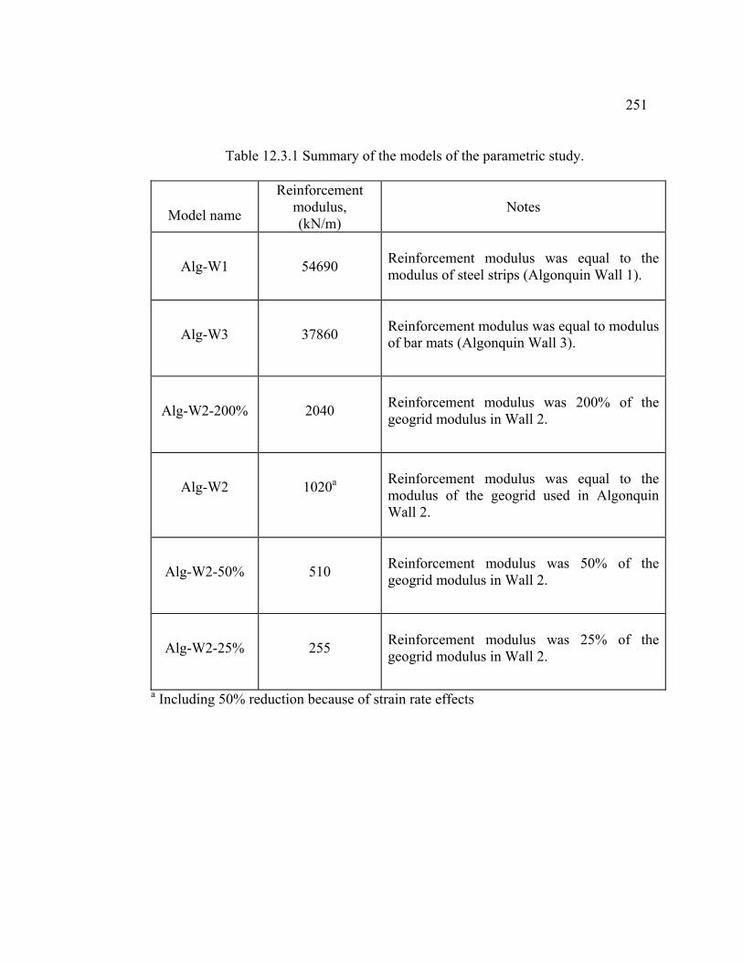
251
Table 12.3.1 Summary of the models of the parametric study.
Model name
Reinforcement modulus, (kN/m)
Notes
Alg-W1
54690
Reinforcement modulus was equal to the modulus of steel strips (Algonquin Wall 1).
Alg-W3
37860
Reinforcement modulus was equal to modulus of bar mats (Algonquin Wall 3).
Alg-W2-200%
2040
Reinforcement modulus was 200% of the geogrid modulus in Wall 2.
Alg-W2
1020a
Reinforcement modulus was equal to the modulus of the geogrid used in Algonquin Wall 2.
Alg-W2-50%
510
Reinforcement modulus was 50% of the geogrid modulus in Wall 2.
Alg-W2-25%
255
Reinforcement modulus was 25% of the geogrid modulus in Wall 2.
a Including 50% reduction because of strain rate effects

252
Figure 12.3.1 Maximum face deflection vs. reinforcement modulus.
Figure 12.3.2 Modeling results showing accumulated inclinometer deflections, at 1.8m
behind wall face.
100
1000
10000
100000
0 10 20 30 40 50 60 70 80 90 100
Maximum Face Deflection (mm)
Rei
nfor
cem
ent M
odul
us,
in Is
olat
ion
(kN
/m)
Parametric Analysis
Survey Measurements
Alg-W2-25%
Alg-W2-50%
Alg-W2, Wall 2
Alg-W3, Wall 3
Alg-W1, Wall 1
Alg-W2-200%
0
1
2
3
4
5
6
0 20 40 60 80 100 120 140 160Inclinometer Deflection (mm)
Hei
ght o
f the
Wal
l (m
)
Alg-W2Alg-W1Alg-W3Alg-W2-200%Alg-W2-50%Alg-W2-25%
253with very high stiffness reinforcement such as steel strips and bar mats (Walls 1 and 3)
had almost the same deflections. This shows that there was a point of diminishing
returns at which increasing reinforcement stiffness did not reduce the overall wall face
deflection.
Figure 12.3.3 summarizes the reinforcement strain distribution obtained for all the
reinforcement stiffnesses analyzed. Both peak strain and overall strain in the
reinforcement increased as the reinforcement stiffness decreased. All the peak strains
occurred at the wall facing except at layer 1 of Model Alg-W2-25% (case with low
reinforcement stiffness). Results of Model Alg-W2-25% showed that the peak strain
of layer 1 was located at about 0.17 m from wall face. Moreover, decreasing the
reinforcement stiffness tended to cause the higher strain zones of the reinforcement to
extend further back from the wall face into the backfill (Figure 12.3.3).
Figure 12.3.4 shows the maximum reinforcement tensions as a function of
reinforcement stiffness. It shows that reinforcement with relatively high stiffness such
as steel reinforcement developed larger reinforcement loads than did low stiffness
reinforcement such as geosynthetics. As shown in Figures 12.3.3 and 12.3.4, as the
reinforcement stiffness decreased sufficiently to result in peak reinforcement strains of
3 to 4% or more, the load in the reinforcement did not continue to decrease; instead, it
began to increase as reinforcement stiffness decreased. Interestingly, based on triaxial

254
Figure 12.3.3 Reinforcement strain distribution.
Layer 7
0
1
2
3
4
0 0.5 1 1.5 2 2.5 3 3.5 4 4.5
Stra
n (%
)
Layer 5
0
1
2
3
4
0 0.5 1 1.5 2 2.5 3 3.5 4 4.5
Stra
n (%
)
Layer 3
0
1
2
3
4
0 0.5 1 1.5 2 2.5 3 3.5 4 4.5
Stra
n (%
)
Layer 1
0
1
2
3
4
0 0.5 1 1.5 2 2.5 3 3.5 4 4.5Distance from Wall Face (m)
Stra
n (%
) Alg-W2 Alg-W1Alg-W3 Alg-W2-200%Alg-W2-50% Alg-W2-25%

255
Figure 12.3.4 Maximum reinforcement tension vs. reinforcement stiffness.
0
2
4
6
8
10
12
100 1000 10000 100000
Reinforcement Modulus, in Isolation (kN/m)
Max
imum
Rei
nfor
cem
ent T
ensi
on(k
N/m
)
layer 1layer 3layer 5layer 7

256tests conducted on this wall backfill (Christopher, 1993), the shear strain
corresponding to the peak shear strength for the soil was on the order of 2 to 4%
strain. Figure 12.3.4 also shows that the maximum reinforcement load occurs in the
middle of the wall (layers 3 and 5) for all the reinforcement stiffnesses analyzed.
12.4 Analyses Matrix of the Major Parametric Study
In order to further investigate the influence of the internal design factors on the
performance of GRS walls, an extensive parametric analysis program was performed.
Internal design factors including soil strength properties, reinforcement stiffness,
reinforcement layer spacing, facing system, and toe restraint were systematically
varied in three fundamental wrapped faced GRS wall models. These models were
modified from numerical models developed for the 3.6m high RMCC test walls, the
6.1m high Algonquin FHWA test walls, and the 12.6m high Rainier Avenue wall.
A total of 256 models were analyzed by systematically introducing combinations
of the controlling factors described above into the three fundamental models. Of these,
72 models failed to reach the final construction stage because internal instability
occurred; thus a total of 184 GRS wall models were fully analyzed in this parametric
study. Table 12.4.1 lists the nine groups of models that were analyzed; each group was
categorized by their heights and facing systems. In each group, backfill soil properties,
reinforcement properties, vertical spacing of reinforcement, and toe restraint were
systematically changed in order to examine the combined influence of these design

257
Table 12.4.1 Model groups of parametric analysis.
Group Wall Height, H (m)
Vertical Spacing, Sv (m)
Facing System
A 12.6 0.38 Wrapped face
B 6.1 0.76 Wrapped face
C 3.6 0.6 Wrapped face
D 6.1 0.38 Wrapped face
E
6.1
0.76
Wrapped face with secondary reinforcement
F 6.1 0.76 Modular block face
G 6.1 0.76 Concrete panel face
H 6.1 0.38 Modular block face
I 6.1 0.38 Concrete panel face

258factors on GRS wall performance. The general boundary conditions, design factors,
and ranges of the design factors are described in the following sections.
12.4.1 General Boundary Conditions and Design Factors
Following are the general boundary conditions and design factors of the models
analyzed in this parametric study:
1. Vertical face—all models had a vertical face because walls with vertical faces had
larger deflections than walls with battered faces.
2. No foundation failure—all model walls were built on a foundation that had good
soil properties; thus bearing capacity failure of the foundation was not a concern of
this analysis.
3. Extended boundary conditions—for all models, the backfill was extended
backward a distance equal to the embeded reinforcement length from the end of
the reinforcement. The foundation soil in front of the wall was also extended a
distance equal to the embedded reinforcement length from the toe of the wall. The
depth of foundation soil was equal to the height of the wall.
4. Uniform reinforcement stiffness and spacing—all layers of reinforcement inside
each model wall had the same stiffness and vertical spacing.

259
5. Ratio of reinforcement length to wall height—all model walls had a reinforcement
length to wall height ratio equal to 0.8.
12.4.2 Controlled Factor I—Backfill Soil Properties
Seven types of granular soils were chosen as the backfill materials for the parametric
analysis. Table 12.4.2 lists the unit weight, friction angle, dilation angle, lateral earth
pressure coefficients, and the parameters of the hyperbolic soil modulus model
described in Chapter 7 (Duncan et al., 1980). These soil properties were set up to
represent good quality backfill (Soil Type VII) to poor quality backfill (Soil Type I)
materials.
12.4.3 Controlled Factor II—Reinforcement Stiffness and Spacing
Reinforcement stiffness (J) in the parametric analysis ranged from 55 kN/m to 60,000
kN/m and represented the reinforcement stiffness of very weak geosynthetics to steel
reinforcement. Three vertical spacings (Sv), 0.38m (1.25ft), 0.76m (2.5ft), and 1.14m
(3.75ft), were used in the parametric analysis models. The correlated global stiffness
(Jg), defined as the reinforcement stiffness divided by the vertical spacing (Christopher
et al., 1990, Christopher, 1993), ranged from 92 kN/m2 to 157,895 kN/m2.

260
Table 12.4.2 Soil properties used in parametric analysis models.
Soil Type
Unit
Weight (kN/m3)
Friction Angle (deg)
Dilation Angle (deg)
Lateral Earth
Pressure Coefficient at
resta, K0
Hyperbolic Soil Modulus
Model Parameters
I 16.68 25 10 0.58 K =800, Rf =0.73, and n =0.5
II 17.66 30 10 0.5 K =1000, Rf =0.73, and n =0.5
III 18.64 35 10 0.43 K =1200, Rf =0.73, and n =0.5
IV 19.62 40 15 0.36 K =1400, Rf =0.73, and n =0.5
V 20.60 45 15 0.29 K =1600, Rf =0.73, and n =0.5
VI 21.58 50 15 0.23 K =1800, Rf =0.73, and n =0.5
VII 22.56 55 20 0.18 K =2100, Rf =0.73, and n =0.5
a Calculated using equation K0 = 1-sinφ.

26112.4.4 Controlled Factor III—Toe Restraint
Four types of toe restraint were used in the parametric models. They are the free toe
(no restraint), toe embedment of 5% of the wall height, toe embedment of 10% of the
wall height, and fixed toe (no displacement allowed).
12.4.5 Controlled Factor IV—Facing Systems
As indicated in Table 12.4.1, four common facing systems of GRS walls were used in
the design of the parametric models. They were wrapped face (Groups A, B, C, and
D), wrapped face with secondary reinforcements (Group E), modular block face
(Group F and H), and concrete panel face (Group G and I). Secondary reinforcement
refers to the short horizontal layers of reinforcement that are inserted in between the
primary reinforcement layers near wall face. The size of the modular block was
190mm in height and 600mm in depth (including the drainage stone column). The
depth of the concrete panel was 140mm. Because FLAC is a two dimensional analysis
program, the width of the structural facing systems was equal to the one unit length of
the models; in this analysis, the length unit of all models was one meter.

26212.5 Analysis Result I—Face Deflection
Because the wall face bulged out in between the reinforcement layers, especially in
models with large reinforcement spacings (Group B and C), only the face deflections
at reinforcement layers were recorded and analyzed. Face deflections of the bulges
were difficult to characterize because plastic failure was found in many soil elements
located in between the reinforcement layers.
In this section, the analysis results are shown as normalized wall height (h/H,
where h is the height at which the deflection was measured and H is the full height of
the wall) versus the face deflections at reinforcement layers (Figures 12.5.1 to 12.5.7).
The influences of soil and geosynthetic reinforcement properties on the distributions
and magnitudes of the face deflections are discussed separately first (Figures 12.5.1 to
12.5.7). A composite material approach is then presented in an effort to summarize the
maximum face deflections with considerations of both soil and reinforcement
properties (Figure 12.5.8). The following observations and conclusions and
discussions about wall face deflections were obtained from the modeling results:
1. Face deflections of GRS walls were found to be affected by the quality of the
backfill. Figures 12.5.1 to 12.5.4 show typical wall deflection results of Groups A,
B, C, and D GRS walls, but with different types of backfill soils. As shown in the
figures, the overall deflections increased as the soil strength decreased.
2632. Face deflections of GRS walls were also found to be affected by the reinforcement
stiffness. Figures 12.5.5 to 12.5.7 show the typical wall deflection results of Group
A, B, C, and D walls that were built using reinforcements with different global
reinforcement stiffnesses. As shown in the figures, the overall deflections increased
as the global stiffness decreased.
3. By comparing Figures 12.5.1, 12.5.4, 12.5.5, and 12.5.6, 12.6 m walls had larger
wall face deflections than 6.1 m walls, even with the same vertical spacing and
reinforcement length to wall height ratio.
4. Walls with smaller vertical spacing deformed less than walls that had the same
height but larger spacings (Figures 12.5.2, 12.5.4, and 12.5.6).
5. Deflection profiles shown in these figures indicate that maximum deflection of
walls with small spacings occurred at the middle of the wall (0.5H, where H is
height of the wall), and maximum deflection of walls with large spacings occurred
at a height about 0.6H.
6. Deflection profiles shown in Figures 12.5.2, 12.5.3, 12.5.6, and 12.5.7 also
indicated that larger deflections occurred at upper half of large spacing walls that
had local failures at wall face. Evidence of tilting of walls with large reinforcement
spacings was observed.

264
Figure 12.5.1 Face deflection profiles of Group A models (wrapped face, H=12.6m,
Sv=0.38m, Jg=1316kN/m2) with soil properties varied.
Figure 12.5.2 Face deflection profiles of Group B models (wrapped face, H=6.1m,
Sv=0.76m, Jg=1312kN/m2) with soil properties varied.
0
0.2
0.4
0.6
0.8
1
0 50 100 150 200 250 300 350 400 450 500Wall Face Deflection (mm)
Nor
mal
ized
Hei
ght (
h/H
)
Soil II
Soil III
Soil IV
Soil V
Soil VI
Soil VII
0
0.2
0.4
0.6
0.8
1
0 50 100 150 200 250 300 350 400 450 500
Wall Face Deflection (mm)
Nor
mal
ized
Hei
ght (
h/H
)Soil I
Soil II
Soil III
Soil IV
Soil V
Soil VI
Soil VII

265
Figure 12.5.3 Face deflection profiles of Group C models (wrapped face, H=3.6m,
Sv=0.6m, Jg=183kN/m2) with soil properties varied.
Figure 12.5.4 Face deflection profiles of Group D models (wrapped face, H=6.1m,
Sv=0.38m, Jg=1316kN/m2) with soil properties varied.
0
0.2
0.4
0.6
0.8
1
0 50 100 150 200 250 300 350 400 450 500
Wall Face Deflection (mm)
Nor
mal
ized
Hei
ght (
h/H
)
Soil II
Soil III
Soil IV
Soil V
Soil VI
Soil VII
0
0.2
0.4
0.6
0.8
1
0 50 100 150 200 250 300 350 400 450 500Wall Face Deflection (mm)
Nor
mal
ized
Hei
ght (
h/H
)
Soil I
Soil II
Soil III
Soil IV
Soil V
Soil VI
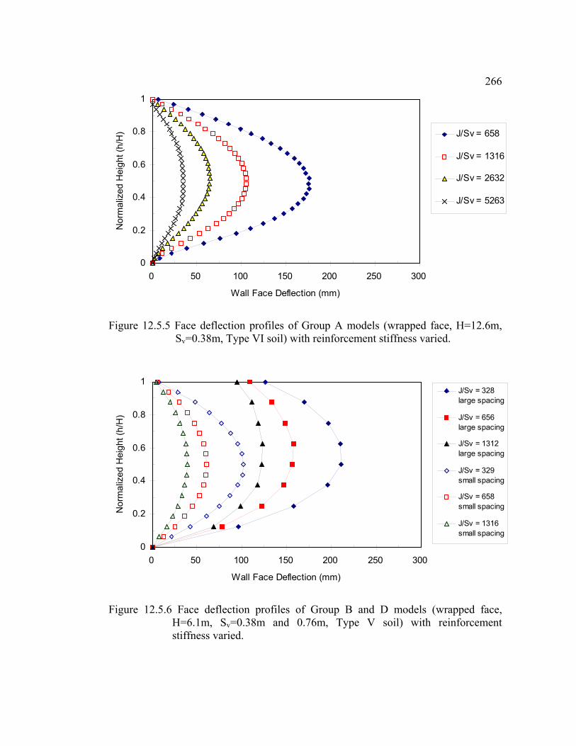
266
Figure 12.5.5 Face deflection profiles of Group A models (wrapped face, H=12.6m,
Sv=0.38m, Type VI soil) with reinforcement stiffness varied.
Figure 12.5.6 Face deflection profiles of Group B and D models (wrapped face,
H=6.1m, Sv=0.38m and 0.76m, Type V soil) with reinforcement stiffness varied.
0
0.2
0.4
0.6
0.8
1
0 50 100 150 200 250 300
Wall Face Deflection (mm)
Nor
mal
ized
Hei
ght (
h/H
) J/Sv = 658
J/Sv = 1316
J/Sv = 2632
J/Sv = 5263
0
0.2
0.4
0.6
0.8
1
0 50 100 150 200 250 300
Wall Face Deflection (mm)
Nor
mal
ized
Hei
ght (
h/H
)
J/Sv = 328large spacing
J/Sv = 656large spacing
J/Sv = 1312large spacing
J/Sv = 329small spacing
J/Sv = 658small spacing
J/Sv = 1316small spacing

2677. Modeling results shown in Figure 12.5.6 indicated that, even when designed with
similar global stiffness, large spacing walls still possessed larger deflections than
the small spacing walls.
In order to summarize the maximum deflections of all model walls with
considerations of both soil and reinforcement properties, the composite GRS modulus
(Ecomp) defined and formulated in Chapter 11 was used (Equation 11.2.7). Figure
12.5.8 shows the normalized maximum wall deflection, maximum deflection (dmax)
divided by the wall height (H), versus the initial composite GRS modulus (Ecomp, ini).
Ecomp, ini was used because most of the face deflections were observed to occur during
construction. To determine the Ecomp, ini, Esoil in Equation 11.2.7 was calculated using
the hyperbolic soil modulus model (Equation 7.1.3) by giving confining pressure
equal to 0.5KoγSv (the confining pressure at middle of each "fresh-placed" lift). The
normalized maximum face deflections showed very good correlation to the Ecomp, ini
for both large spacing and small spacing walls (Figure 12.5.8). Results shown in
Figure 12.5.8 indicated that the normalized maximum deflections increased as the
Ecomp, ini decreased.
sv
comp ESJE += (Eq. 11.2.7)

268
Figure 12.5.7 Face deflection profiles of Group C models (wrapped face, H=3.6m,
Sv=0.6m, Type V soil) with reinforcement stiffness varied.
Figure 12.5.8 Initial GRS composite modulus versus the normalized maximum face
deflection.
0
0.2
0.4
0.6
0.8
1
0 50 100 150 200 250 300
Wall Face Deflection (mm)
Nor
mal
ized
Hei
ght (
h/H
) J/Sv = 92
J/Sv = 183
J/Sv = 417
J/Sv = 833
J/Sv = 1667
y = 5E+12x-2.9955
R2 = 0.8895
y = 1E+11x-2.4068
R2 = 0.7503
0
10
20
30
40
50
60
70
80
0 2000 4000 6000 8000 10000 12000 14000 16000 18000 20000
Initial GRS Composite Modulus (kN/m^2)
Nor
mal
ized
Max
imum
Fac
e D
efle
ctio
n (m
m/m
)
Small Sv, No Local FailureLarge Sv, Local Failure

269Also shown in Figure 12.5.8, for the small spacing walls, the maximum deflections
increased rapidly even with a small decrease in Ecomp, ini when the Ecomp, ini had values
smaller than 8,000 kN/m2. For the large spacing walls, the normalized maximum
deflection increased rapidly with a small deduction of Ecomp, ini as soon as the Ecomp, ini
was smaller than 10,000 kN/m2.
12.6 Analysis Result II—Reinforcement Tension
12.6.1 Characterization of Reinforcement Tensions
Figure 12.6.1 shows the typical results of reinforcement tension distributions along
a reinforcement layer. As shown in Figure 12.6.1, Tpeak was defined as the maximum
reinforcement tension along the reinforcement layer, and Tave was defined as the
average reinforcement tension of each layer. Because the reinforcement elements
inside numerical models used in this parametric study were attached to the material
element nodes, as described in Section 8.5.6, these numerical models tended to
overpredict Tpeak at the face of the wrapped face wall or the connections of the
structural faced wall. Figure 12.6.2 shows typical distributions of both Tpeak and Tave.
The maximum value of Tpeak of all layers inside a GRS wall was defined as Tpeak_max,
and the maximum value of Tave of All layers was defined as Tave_max.
As shown in Figure 12.6.2, distributions of Tpeak and locations of Tpeak, max are
more difficult to characterize than Tave. In this study, in order to analyze the influences
of both soil and reinforcement properties on the overall reinforcement tension
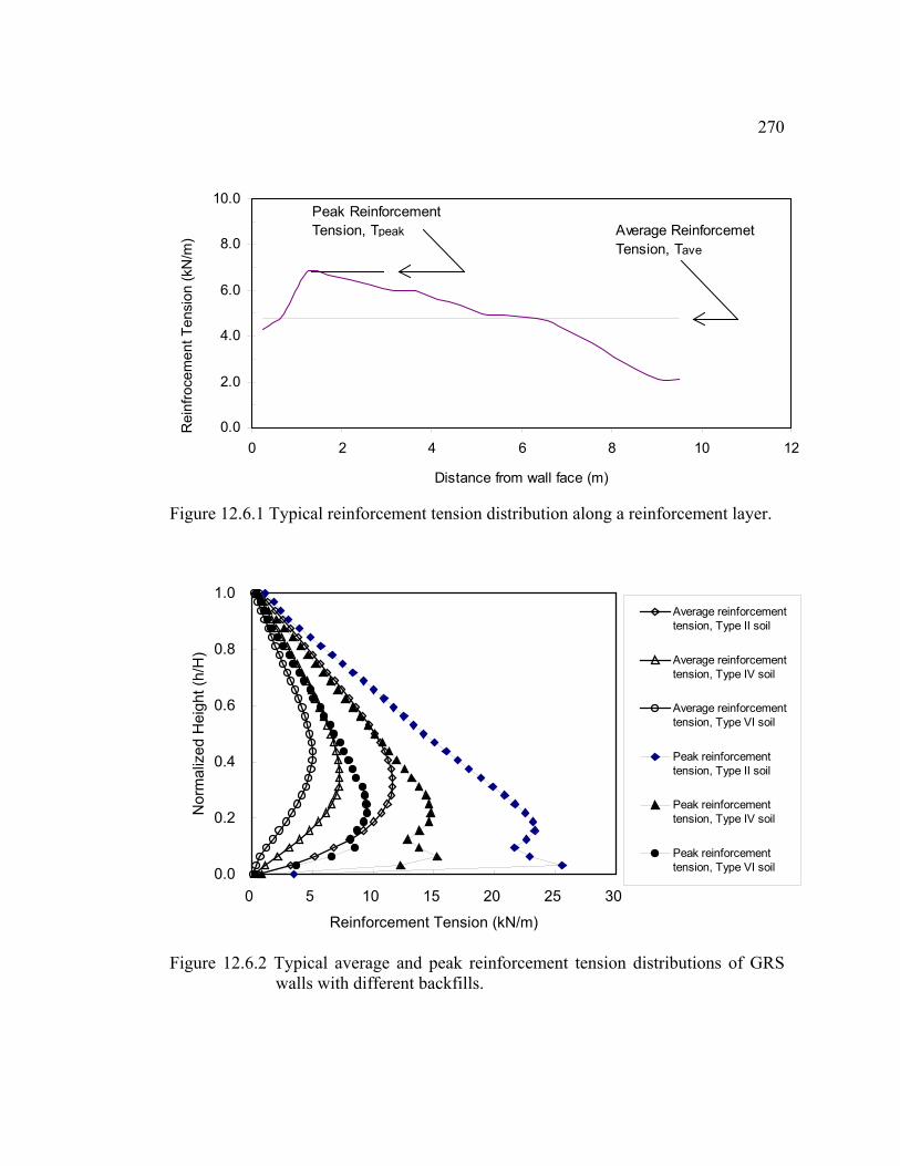
270
Figure 12.6.1 Typical reinforcement tension distribution along a reinforcement layer.
Figure 12.6.2 Typical average and peak reinforcement tension distributions of GRS walls with different backfills.
0.0
2.0
4.0
6.0
8.0
10.0
0 2 4 6 8 10 12
Distance from wall face (m)
Rei
nfro
cem
ent T
ensi
on (k
N/m
) Average Reinforcemet Tension, Tave
Peak Reinforcement Tension, Tpeak
0.0
0.2
0.4
0.6
0.8
1.0
0 5 10 15 20 25 30
Reinforcement Tension (kN/m)
Nor
mal
ized
Hei
ght (
h/H
)
Average reinforcementtension, Type II soil
Average reinforcementtension, Type IV soil
Average reinforcementtension, Type VI soil
Peak reinforcementtension, Type II soil
Peak reinforcementtension, Type IV soil
Peak reinforcementtension, Type VI soil

271distributions, analysis results were presented using Tave. As shown in Figures 12.6.3 to
12.6.11, distributions of Tave of Groups A, B, C, and D models with different soil
properties or reinforcement properties were plotted versus the normalized height.
Relations between Tpeak_max and Tave_max of different GRS walls are discussed in
Chapter 14.
12.6.2 Analysis Results
The influences of the soil and reinforcement properties on the magnitudes and
distributions of Tave, as well as on the locations of the Tave_max, can be summarized as
follows:
1. Tave was found to be affected by the quality of the backfill soils. Figures 12.6.3 to
12.6.6 show the Tave distributions of Group A, B, C, D walls with different types of
backfill soils. As shown in the figures, the overall reinforcement tensions increased
as the soil strength decreased.
2. Tave was also found to be affected by the reinforcement stiffness. Figures 12.6.7 to
12.6.10 show the Tave distributions of Group A, B, C, and D walls that were
designed with different global reinforcement stiffnesses. Results shown in these
figures indicate that the overall reinforcement tensions increased as the
reinforcement stiffness increased.

272
Figure 12.6.3 Reinforcement tension distributions of Group A models (wrapped face,
H=12.6m, Sv=0.38m, Jg=1316kN/m2) with soil properties varied.
Figure 12.6.4 Reinforcement tension distributions of Group B models (wrapped face,
H=6.1m, Sv=0.76m, Jg=1312kN/m2) with soil properties varied.
0
0.2
0.4
0.6
0.8
1
0 2 4 6 8 10 12 14 16 18 20
Average Reinforcement Tension (kN/m)
Nor
mal
ized
Hei
ght (
h/H
)Soil I
Soil II
Soil III
Soil IV
Soil V
Soil VI
Soil VII
0
0.2
0.4
0.6
0.8
1
0 2 4 6 8 10 12 14 16 18 20Average Reinforcement Tension (kN/m)
Nor
mal
ized
Hei
ght (
h/H
)
Soil II
Soil III
Soil IV
Soil V
Soil VI
Soil VII
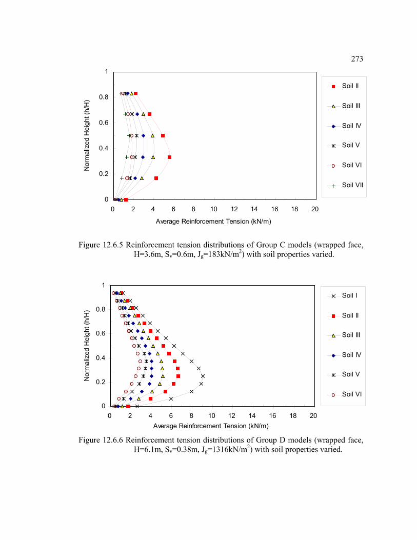
273
Figure 12.6.5 Reinforcement tension distributions of Group C models (wrapped face,
H=3.6m, Sv=0.6m, Jg=183kN/m2) with soil properties varied.
Figure 12.6.6 Reinforcement tension distributions of Group D models (wrapped face, H=6.1m, Sv=0.38m, Jg=1316kN/m2) with soil properties varied.
0
0.2
0.4
0.6
0.8
1
0 2 4 6 8 10 12 14 16 18 20
Average Reinforcement Tension (kN/m)
Nor
mal
ized
Hei
ght (
h/H
)Soil II
Soil III
Soil IV
Soil V
Soil VI
Soil VII
0
0.2
0.4
0.6
0.8
1
0 2 4 6 8 10 12 14 16 18 20Average Reinforcement Tension (kN/m)
Nor
mal
ized
Hei
ght (
h/H
)
Soil I
Soil II
Soil III
Soil IV
Soil V
Soil VI

274
Figure 12.6.7 Reinforcement tension distributions of Group A models (wrapped face,
H=12.6m, Sv=0.38m, Type VI soil) with reinforcement stiffness varied.
Figure 12.6.8 Reinforcement tension distributions of Group B models (wrapped face,
H=6.1m, Sv= 0.76m, Type V soil) with reinforcement stiffness varied.
0
0.2
0.4
0.6
0.8
1
0 2 4 6 8 10
Average Reinforcement Tension (kN/m)
Nor
mal
ized
Hei
ght (
h/H
) J/Sv = 658
J/Sv = 1316
J/Sv = 2632
J/Sv = 5263
0
0.2
0.4
0.6
0.8
1
0 2 4 6 8 10
Average Reinforcement Tension (kN/m)
Nor
mal
ized
Hei
ght (
h/H
)
J/Sv = 328
J/Sv = 656
J/Sv = 1312
J/Sv = 3937
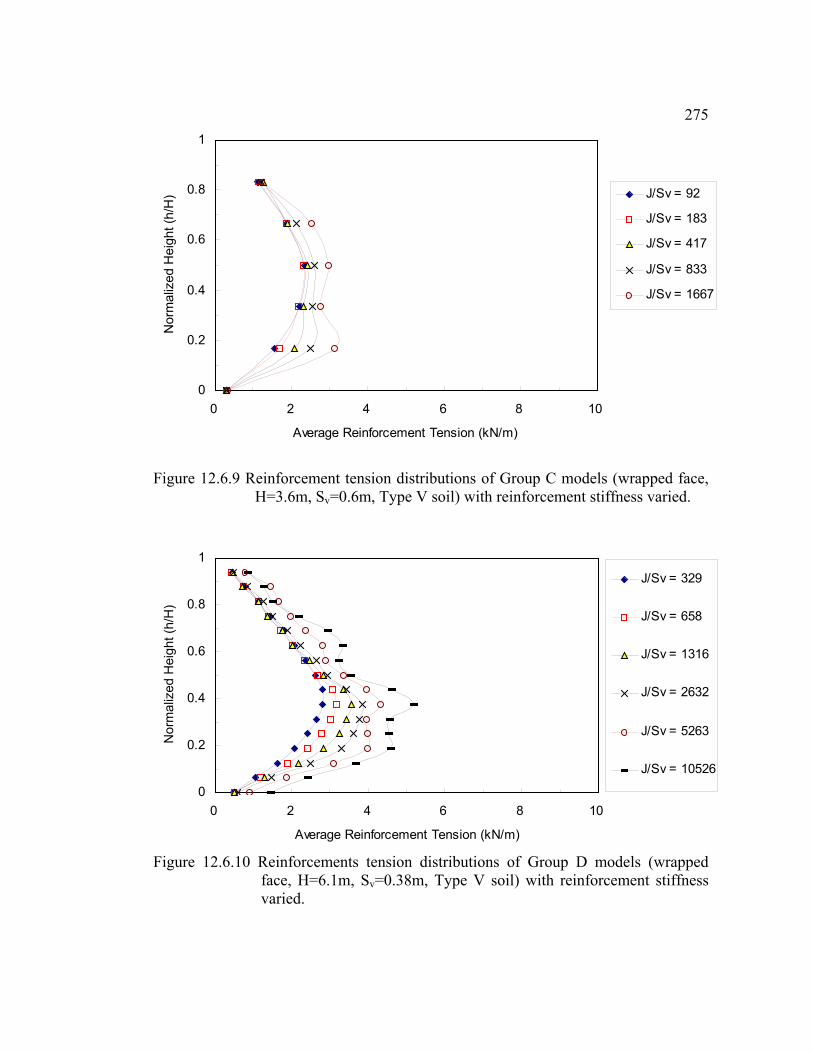
275
Figure 12.6.9 Reinforcement tension distributions of Group C models (wrapped face,
H=3.6m, Sv=0.6m, Type V soil) with reinforcement stiffness varied.
Figure 12.6.10 Reinforcements tension distributions of Group D models (wrapped face, H=6.1m, Sv=0.38m, Type V soil) with reinforcement stiffness varied.
0
0.2
0.4
0.6
0.8
1
0 2 4 6 8 10
Average Reinforcement Tension (kN/m)
Nor
mal
ized
Hei
ght (
h/H
) J/Sv = 92
J/Sv = 183
J/Sv = 417
J/Sv = 833
J/Sv = 1667
0
0.2
0.4
0.6
0.8
1
0 2 4 6 8 10
Average Reinforcement Tension (kN/m)
Nor
mal
ized
Hei
ght (
h/H
)
J/Sv = 329
J/Sv = 658
J/Sv = 1316
J/Sv = 2632
J/Sv = 5263
J/Sv = 10526

276
Figure 12.6.11 Reinforcements tension distributions of walls with different spacings
(Group B and D).
0
0.2
0.4
0.6
0.8
1
0 2 4 6 8 10
Average Reinforcement Tension (kN/m)
Nor
mal
ized
Hei
ght (
h/H
)
J/Sv = 328large spacing
J/Sv = 656large spacing
J/Sv = 1312large spacing
J/Sv = 329small spacing
J/Sv = 658small spacing
J/Sv = 1316small spacing

2773. Modeling results shown in Figures 12.6.3, 12.6.6, 12.6.7 and 12.6.10 indicate that
the Tave distributions of Group A and D (small spacing, wrapped face walls) had a
triangular shape. As shown in the figures, Tave first increased as the height of the
wall increased. It reached its maximum values at the middle to one-third of the
height of the walls, and then started to decrease as the height increased.
4. Locations of the maximum average reinforcement tensions (Tave_max) were found to
be affected by the quality of the backfill soils rather than the reinforcement
stiffnesses. As shown in Figures 12.6.3 to 12.6.6, locations of Tave_max varied from
0.5H (Type VII soil) to 0.3H (Type I soil). No noticeable changes of Tave_max
locations were found for walls that were designed using the same backfill soil but
with different reinforcement stiffnesses (Figures 12.6.7 to 12.6.10).
5. Results in Figures 12.6.7, 12.6.8, and 12.6.10 show that the reinforcement tensions
in the upper half of the walls did not increase very much as the global reinforcement
stiffnesses increased from 329 to 2632 kN/m2. However, reinforcement tensions in
the lower half of the wall as well as Tave_max did increase as the global reinforcement
stiffnesses increased.
6. The large spacing walls (Group B) possessed higher reinforcement tensions than
small spacing walls (Group D), even though the walls were designed with similar
global reinforcement stiffnesses (Figure 12.6.11).

27812.7 Analysis Result III—Effects of Toe Restraint
The major purpose of designing GRS walls with toe restraint is to increase the sliding
resistance. However, the influence of the toe restraint on the performance of GRS
walls was not carefully examined before. In this study, different degrees of toe
restraints were added on the three fundamental models to investigate the influence of
the toe restraints on performance of GRS walls. Moreover, quality of the backfill of
these models was also varied to further examine the correlation between the degree of
the influence of toe restraints and the backfill qualities. Results of these toe-restraint
models were presented in the similar formats as the modeling results presented in
previous sections, i.e. normalized height versus face deflection profiles or average
reinforcement tension distributions.
Both face deflections and reinforcement tension distributions of GRS walls were
found to be affected by different degrees of toe restraint. Figures 12.7.1 to 12.7.3 show
the typical face deflection results of the walls that were designed with different types
of toe restraints compared to the walls without any toe restraint. Figures 12.7.4 to
12.7.6 show the influence of different toe restraints (no restraint, 0.05H embedment,
0.1H embedment, and fixed toe) on the reinforcement tension distributions.
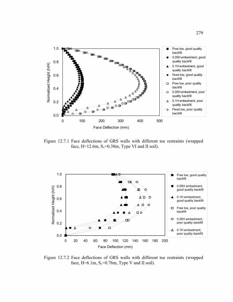
279
Figure 12.7.1 Face deflections of GRS walls with different toe restraints (wrapped
face, H=12.6m, Sv=0.38m, Type VI and II soil).
Figure 12.7.2 Face deflections of GRS walls with different toe restraints (wrapped face, H=6.1m, Sv=0.76m, Type V and II soil).
0.0
0.2
0.4
0.6
0.8
1.0
0 100 200 300 400 500
Face Deflection (mm)
Nor
mal
ized
Hei
ght (
h/H
)Free toe, good qualitybackfill0.05H embedment, goodquality backfill0.1H embedment, goodquality backfillf ixed toe, good qualitybackfillFree toe, poor qualitybackfill0.05H embedment, poorquality backfill0.1H embedment, poorquality backfillFixed toe, poor qualitybackfill
0.0
0.2
0.4
0.6
0.8
1.0
0 20 40 60 80 100 120 140 160 180 200Face Deflection (mm)
Nor
mal
ized
Hei
ght (
h/H
)
Free toe, good qualitybackfill
0.05H embedment,good quality backfill
0.1H embedment,good quality backfill
Free toe, poor qualitybackfill
0.05H embedment,poor quality backfill
0.1H embedment,poor quality backfill
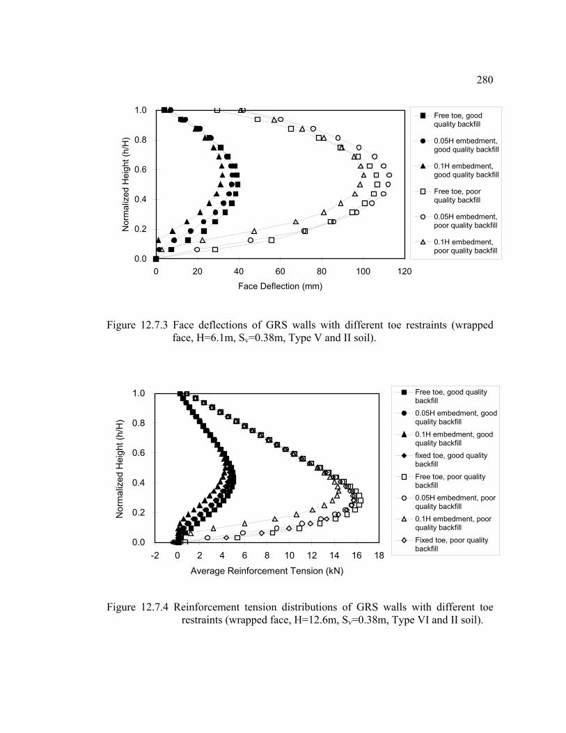
280
Figure 12.7.3 Face deflections of GRS walls with different toe restraints (wrapped
face, H=6.1m, Sv=0.38m, Type V and II soil).
Figure 12.7.4 Reinforcement tension distributions of GRS walls with different toe
restraints (wrapped face, H=12.6m, Sv=0.38m, Type VI and II soil).
0.0
0.2
0.4
0.6
0.8
1.0
0 20 40 60 80 100 120Face Deflection (mm)
Nor
mal
ized
Hei
ght (
h/H
)Free toe, goodquality backfill
0.05H embedment,good quality backfill
0.1H embedment,good quality backfill
Free toe, poorquality backfill
0.05H embedment,poor quality backfill
0.1H embedment,poor quality backfill
0.0
0.2
0.4
0.6
0.8
1.0
-2 0 2 4 6 8 10 12 14 16 18Average Reinforcement Tension (kN)
Nor
mal
ized
Hei
ght (
h/H
)
Free toe, good qualitybackfill0.05H embedment, goodquality backfill0.1H embedment, goodquality backfillfixed toe, good qualitybackfillFree toe, poor qualitybackfill0.05H embedment, poorquality backfill0.1H embedment, poorquality backfillFixed toe, poor qualitybackfill

281
Figure 12.7.5 Reinforcement tension distributions of GRS walls with different toe
restraints (wrapped face, H=6.1m, Sv=0.76m, Type V and II soil).
Figure 12.7.6 Reinforcement tension distributions of GRS walls with different toe
restraints (wrapped face, H=6.1m, Sv=0.38m, Type V and II soil).
0.0
0.2
0.4
0.6
0.8
1.0
-2 0 2 4 6 8 10 12 14 16 18Average Reinforcement Tension (kN)
Nor
mal
ized
Hei
ght (
h/H
)Free toe, good qualitybackfill
0.05H embedment,good quality backfill
0.1H embedment, goodquality backfill
Free toe, poor qualitybackfill
0.05H embedment,poor quality backfill
0.1H embedment, poorquality backfill
0.0
0.2
0.4
0.6
0.8
1.0
-2 0 2 4 6 8 10 12 14 16 18
Average Reinforcement Ttension (kN)
Nor
mal
ized
Hei
ght (
h/H
Free toe, good qualitybackfill
0.05H embedment,good quality backfill
0.1H embedment,good quality backfill
Free toe, poor qualitybackfill
0.05H embedment,poor quality backfill
0.1H embedment, poorquality backfill
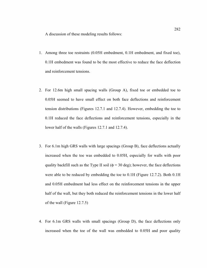
282A discussion of these modeling results follows:
1. Among three toe restraints (0.05H embedment, 0.1H embedment, and fixed toe),
0.1H embedment was found to be the most effective to reduce the face deflection
and reinforcement tensions.
2. For 12.6m high small spacing walls (Group A), fixed toe or embedded toe to
0.05H seemed to have small effect on both face deflections and reinforcement
tension distributions (Figures 12.7.1 and 12.7.4). However, embedding the toe to
0.1H reduced the face deflections and reinforcement tensions, especially in the
lower half of the walls (Figures 12.7.1 and 12.7.4).
3. For 6.1m high GRS walls with large spacings (Group B), face deflections actually
increased when the toe was embedded to 0.05H, especially for walls with poor
quality backfill such as the Type II soil (φ = 30 deg); however, the face deflections
were able to be reduced by embedding the toe to 0.1H (Figure 12.7.2). Both 0.1H
and 0.05H embedment had less effect on the reinforcement tensions in the upper
half of the wall, but they both reduced the reinforcement tensions in the lower half
of the wall (Figure 12.7.5)
4. For 6.1m GRS walls with small spacings (Group D), the face deflections only
increased when the toe of the wall was embedded to 0.05H and poor quality

283backfill (Type I soil) was used (Figure 12.7.3). When the wall was built with good
quality backfill (Type V soil), embedding the toe to 0.05H could still reduce the
face deflections (Figure 12.7.3). Both 0.1H and 0.05H embedment had less effect
on the reinforcement tensions at upper half of the wall, but they were able to
reduce the reinforcement tensions at lower half of the wall (Figure 12.7.6).

28412.8 Analysis Result IV—Effects of Different Facing Systems
Three common wall facing systems, a wrapped face with secondary reinforcement, a
modular block face, and a concrete panel face, were added to 6.1m high wrapped face
models, including Group B (Sv = 0.76m) and Group D (Sv = 0.38m) models. Effects of
these facing systems on the wall face deflections as well as reinforcement tension
distributions were analyzed and compared to those of the wrapped face walls. Results
of models with different facing systems were presented in the similar formats as the
results of wrapped face walls presented in Sections 12.5 and 12.6—normalized height
versus face deflection profiles and average reinforcement tension distributions.
The following points summarize the results of these analyses:
1. As shown in Figure 12.8.1, maximum wall deflections of the wrapped face walls
can be reduced by using all three facing systems, especially for the large spacing
walls.
2. Wrapped face walls designed with secondary reinforcements were found to have
results similar to those walls with structural facing systems when the Ecomp of their
backfills was higher than about 10,500 kN/m2 (Figure 12.8.1). Secondary
reinforcement provided less improvement to the face deflection for walls that had
Ecomp lower than about 10,500 kN/m2 (Figure 12.8.1).
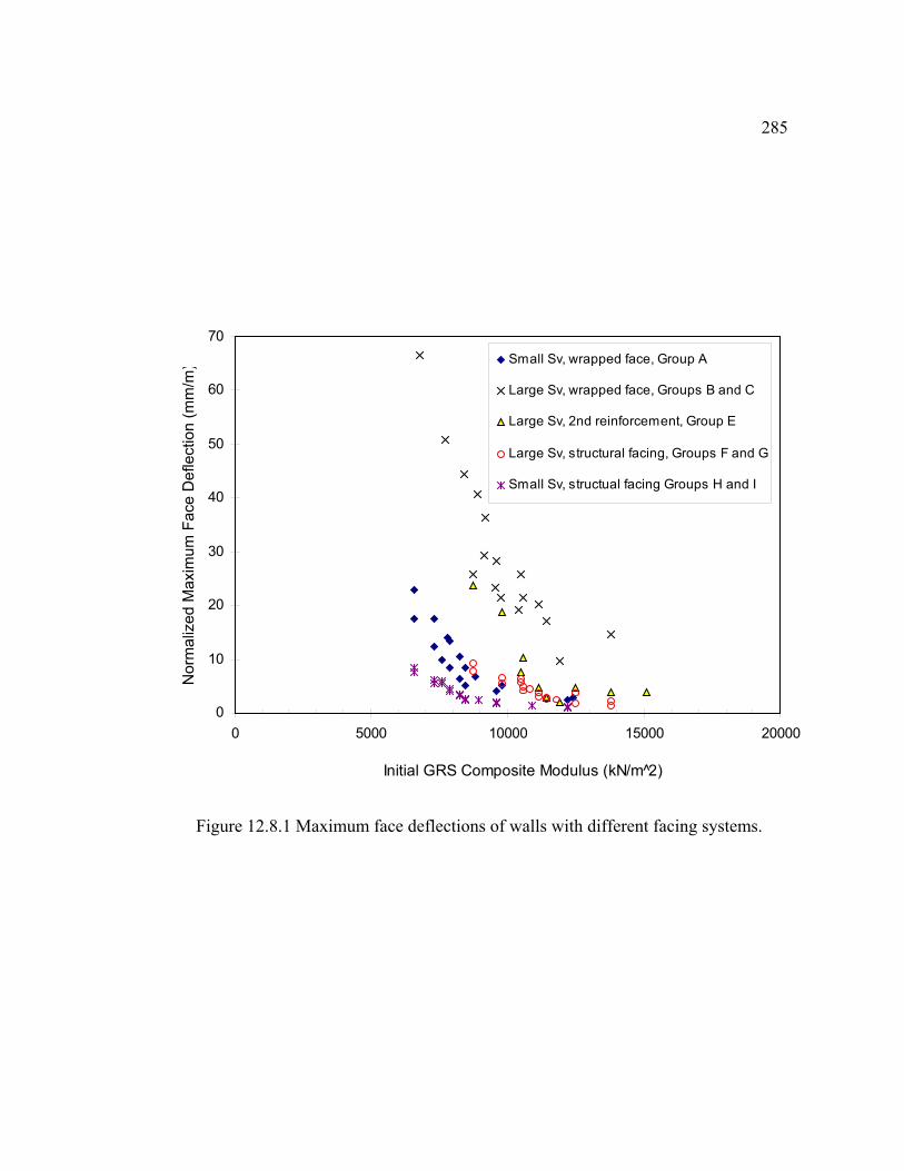
285
Figure 12.8.1 Maximum face deflections of walls with different facing systems.
0
10
20
30
40
50
60
70
0 5000 10000 15000 20000
Initial GRS Composite Modulus (kN/m 2̂)
Nor
mal
ized
Max
imum
Fac
e D
efle
ctio
n (m
m/m
) Small Sv, wrapped face, Group A
Large Sv, wrapped face, Groups B and C
Large Sv, 2nd reinforcement, Group E
Large Sv, structural facing, Groups F and G
Small Sv, structual facing Groups H and I

2863. By using the structural facing systems such as modular blocks and concrete panels,
the face deflections of walls with large spacing were similar to small spacing
wrapped face walls (Figure 12.8.1). For small spacing walls, the maximum face
deflections were also reduced with the aid of the structural facing systems;
however, the improvement was not as great as for the large spacing walls (Figure
12.8.1).
4. As shown in Figures 12.8.2 and 12.8.3, for most cases analyzed, the reinforcement
tensions inside the wrapped face GRS walls were able to be reduced using the
secondary reinforcement. However, for walls with weak backfill (Type II soil),
secondary reinforcement not only increased the reinforcement tension but also
raised the elevation of the maximum reinforcement tension (Figure 12.8.2).
5. Results of Figures 12.8.4, 12.8.5, 12.8.6, and 12.8.7 indicated that the modular
block face was able to decrease the reinforcement tensions of both large and small
spacing wrapped face walls. Especially for walls with weak backfill such as Type
II soil, great improvements were found for both large and small spacing walls
(Figures 12.8.4 and 12.8.6).
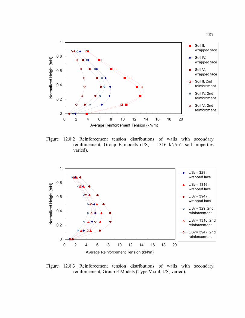
287
Figure 12.8.2 Reinforcement tension distributions of walls with secondary
reinforcement, Group E models (J/Sv = 1316 kN/m2, soil properties varied).
Figure 12.8.3 Reinforcement tension distributions of walls with secondary
reinforcement, Group E Models (Type V soil, J/Sv varied).
0
0.2
0.4
0.6
0.8
1
0 2 4 6 8 10 12 14 16 18 20Average Reinforcement Tension (kN/m)
Nor
mal
ized
Hei
ght (
h/H
)Soil II,wrapped face
Soil IV,wrapped face
Soil VI,wrapped face
Soil II, 2ndreinforcment
Soil IV, 2ndreinforcment
Soil VI, 2ndreinforcment
0
0.2
0.4
0.6
0.8
1
0 2 4 6 8 10 12 14 16 18 20
Average Reinforcement Tension (kN/m)
Nor
mal
ized
Hei
ght (
h/H
)
J/Sv = 329,wrapped face
J/Sv = 1316,wrapped face
J/Sv = 3947,wrapped face
J/Sv = 329, 2ndreinforcement
J/Sv = 1316, 2ndreinforcement
J/Sv = 3947, 2ndreinforcement

288
Figure 12.8.4 Reinforcement tension distributions of walls with modular block face,
Group F models (Sv = 0.76m, J/Sv = 1316 kN/m2, soil properties varied).
Figure 12.8.5 Reinforcement tension distributions of walls with modular block face,
Group F models (Sv = 0.76m, Type V soil, J/Sv varied).
0
0.2
0.4
0.6
0.8
1
0 2 4 6 8 10 12 14 16 18 20Average Reinforcement Tension (kN/m)
Nor
mal
ized
Hei
ght (
h/H
)Soil II, wrappedface
Soil IV, wrappedface
Soil VI, wrappedface
Soil II, modularblock face
Soil IV, modularblock face
Soil VI, modularblock face
0
0.2
0.4
0.6
0.8
1
0 2 4 6 8 10 12 14 16 18 20
Average Reinforcement Tension (kN/m)
Nor
mal
ized
Hei
ght (
h/H
)
J/Sv = 329,wrapped face
J/Sv = 1316,wrapped face
J/Sv = 3947,wrapped face
J/Sv = 329, modularblock face
J/Sv = 1316,modular block face
J/Sv = 3947,modular block face
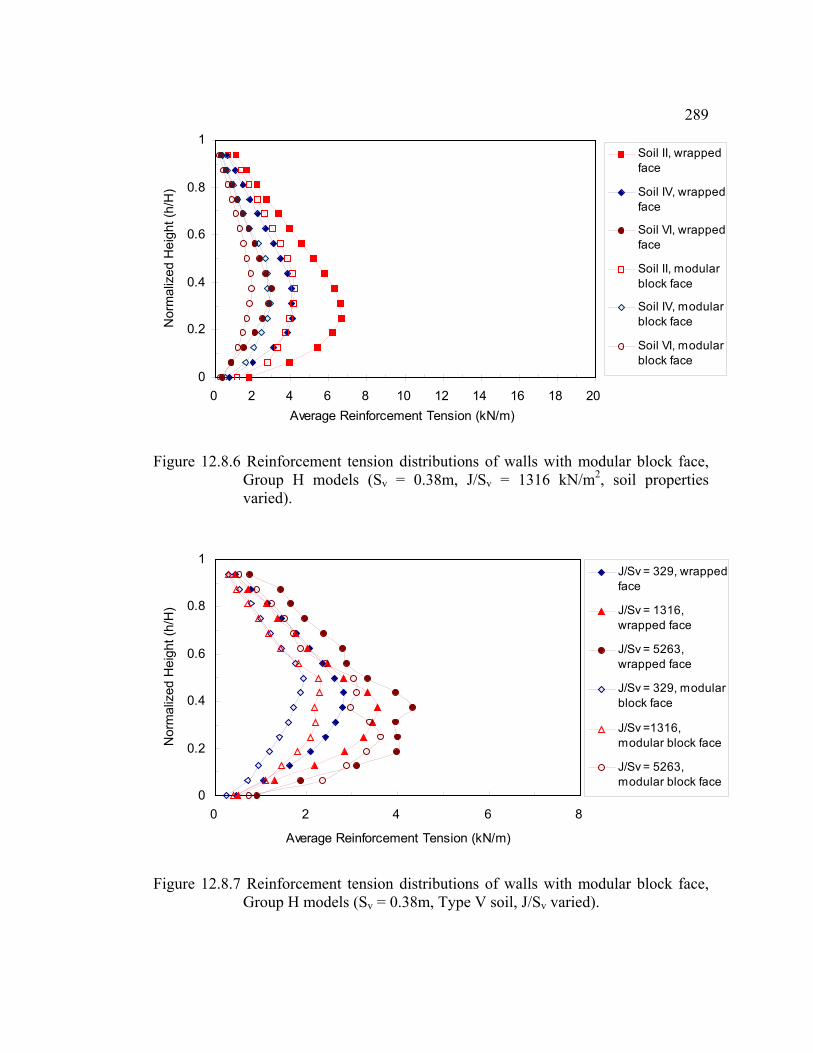
289
Figure 12.8.6 Reinforcement tension distributions of walls with modular block face,
Group H models (Sv = 0.38m, J/Sv = 1316 kN/m2, soil properties varied).
Figure 12.8.7 Reinforcement tension distributions of walls with modular block face,
Group H models (Sv = 0.38m, Type V soil, J/Sv varied).
0
0.2
0.4
0.6
0.8
1
0 2 4 6 8 10 12 14 16 18 20Average Reinforcement Tension (kN/m)
Nor
mal
ized
Hei
ght (
h/H
)Soil II, wrappedface
Soil IV, wrappedface
Soil VI, wrappedface
Soil II, modularblock face
Soil IV, modularblock face
Soil VI, modularblock face
0
0.2
0.4
0.6
0.8
1
0 2 4 6 8
Average Reinforcement Tension (kN/m)
Nor
mal
ized
Hei
ght (
h/H
)
J/Sv = 329, wrappedface
J/Sv = 1316,wrapped face
J/Sv = 5263,wrapped face
J/Sv = 329, modularblock face
J/Sv =1316,modular block face
J/Sv = 5263,modular block face

290
Figure 12.8.8 Reinforcement tension distributions of walls with concrete panel face,
Group G models (Sv = 0.76m, J/Sv = 1316 kN/m2, soil properties varied).
Figure 12.8.9 Reinforcement tension distributions of walls with concrete panel face,
Group G models (Sv = 0.76m, Type V soil, J/Sv varied).
0
0.2
0.4
0.6
0.8
1
0 2 4 6 8 10 12 14 16 18 20Average Reinforcement Tension (kN/m)
Nor
mal
ized
Hei
ght (
h/H
)Soil II, wrappedface
Soil IV, wrappedface
Soil VI, wrappedface
Soil II, concretepanel face
Soil IV, concretepanel face
Soil VI, concretepanel face
0
0.2
0.4
0.6
0.8
1
0 2 4 6 8 10 12 14 16 18 20
Average Reinforcement Tension (kN/m)
Nor
mal
ized
Hei
ght (
h/H
)
J/Sv = 329, wrappedface
J/Sv = 1316,wrapped face
J/Sv = 3947,wrapped face
J/Sv = 329, concretepanel face
J/Sv = 1316,concrete panel face
J/Sv = 3947,concrete panel face

291
Figure 12.8.10 Reinforcement tension distributions of walls with concrete panel face,
Group I models (Sv = 0.38m, J/Sv = 1316 kN/m2, soil properties varied).
Figure 12.8.11 Reinforcement tension distributions of walls with concrete panel face,
Group I models (Sv = 0.38m, Type V soil, J/Sv varied)
0
0.2
0.4
0.6
0.8
1
0 2 4 6 8Average Reinforcement Tension (kN/m)
Nor
mal
ized
Hei
ght (
h/H
)Soil II, wrappedface
Soil IV, wrappedface
Soil VI, wrappedface
Soil II, concretepanel face
Soil IV, concretepanel face
Soil VI, concretepanel face
0
0.2
0.4
0.6
0.8
1
0 2 4 6 8 10 12 14 16 18 20
Average Reinforcement Tension (kN/m)
Nor
mal
ized
Hei
ght (
h/H
)
J/Sv = 329, wrappedface
J/Sv = 1316,wrapped face
J/Sv = 5263,wrapped face
J/Sv = 329, concretepanel face
J/Sv =1316,concrete panel face
J/Sv = 5263,concrete panel face
2926. Performance of the concrete panel faced walls was found to be very similar to that
of modular block faced walls. Figures 12.8.8, 12.8.9, 12.8.10, and 12.8.11
indicated that the concrete panel face was able to decrease the reinforcement
tensions of both large and small spacing wrapped face walls. Improvements were
also found for walls with weak backfill (Figures 12.8.4 and 12.8.6).
12.9 Summary and Conclusions
1. Local failures were observed near the faces of GRS walls with larger vertical
reinforcement spacings. For wrapped face GRS walls that were designed with the
same global stiffnesses but different vertical reinforcement spacings, the large
spacing walls exhibited much higher face deflections than the small spacing ones
(Figure 12.5.5).
2. Face deformation of GRS walls was found to be affected by both the strength
properties of the backfill and the global reinforcement stiffness. Parametric analysis
results shown in Section 12.5 indicated that face deflections of GRS walls increased
as the soil strength properties decreased. Face deflections decreased as the global
reinforcement stiffness increased. A good correlation was found between the GRS
composite modulus (Ecomp) and normalized maximum face deflection (dmax/H)
(Figures 12.5.8 and 12.8.1).
3. Reinforcement tensions in GRS walls were also found to be affected by both the
strength properties of the backfill and the global reinforcement stiffness. Parametric

293analysis results shown in Section 12.6 indicated that overall reinforcement tensions
in the GRS walls increased as the soil strength properties decreased. Overall
reinforcement tensions also increased as the global reinforcement stiffness
increased. However, the reinforcement tensions started to increase when the walls
were designed using very weak reinforcement because of the large strains exhibited
(Figure 12.3.4).
4. Toe restraint was able to reduce the maximum face deflections and reinforcement
tensions (Figures 12.7.1 to 12.7.6). Among three toe restraints (0.05H embedment,
0.1H embedment, and fixed toe), 0.1H embedment was found to be the most
effective toe condition to improve the performance of GRS walls, especially for
walls designed with poor quality backfill.
5. For large spacing walls, secondary reinforcement was found to be only effective for
improving performance of walls with good quality backfill. Both face deflections
and reinforcement tensions of GRS walls with good quality backfill could be
decreased using secondary reinforcement (Figures 12.8.1, 12.8.2 and 12.8.3).
6. Structural facing systems such as modular blocks and concrete panels were able to
improve the stability and reduce the deformation of GRS walls, especially walls
with large spacings. Using structural facing systems could reduce maximum face
deflections (Figure 12.8.1) as well as reinforcement tensions (Figures 12.8.4 to
12.8.11) of both large and small spacing wrapped face walls.

294
7. In contrast to the tie-back wedge method that predicts a maximum reinforcement
tension at the bottom of the wall, results of the parametric analyses indicated that
locations of the maximum overall (average) reinforcement tensions occurred
between 0.25H (poor quality backfill) to 0.5H (good quality backfill).

295Chapter 13
Anisotropic Model for Geosynthetic Reinforced Soil Composite
Properties
Instead of analyzing the geosynthetic reinforcement and soil separately, an effort was
made in this research to develop numerical analyses based on composite material
concepts. In the composite approach, the GRS element was considered to be a
reinforced composite material. Theory of anisotropic material under plane strain
loading conditions described in Chapter 4 was used to analyze the different stress-
strain behavior in the different principal directions of the GRS composite. The author
has published preliminary results of this research (Holtz and Lee, 1997; Lee and
Holtz, 1998).
13.1 Behavior of Geosynthetic Reinforced Soil Element
For a GRS element shown in Figure 13.1.1, different reinforcing mechanisms have
been found in different principal directions (Hausmann, 1990; Boyle, 1995). In the
horizontal directions, soil is reinforced by the tensile forces developed along the
geosynthetic and then transmitted into the soil. In the vertical direction, soil is also
reinforced because additional resistance to the gravity force is provided by the
horizontally placed reinforcement. In Figure 13.1.1, the vertical direction is defined as
direction 1 and the horizontal directions are defined as directions 2 and 3. The
geosynthetic reinforcement is placed on a plane perpendicular to direction 1 but also
parallel to directions 2 and 3. Therefore, the different reinforcing mechanisms of a
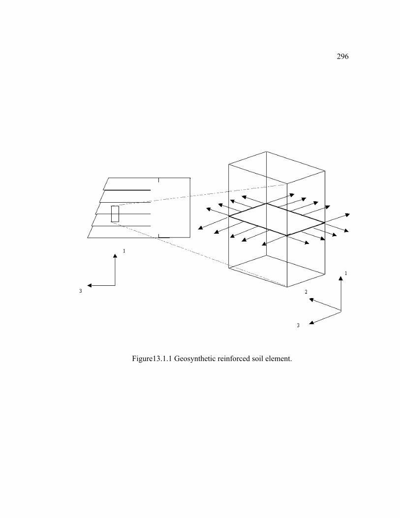
296
Figure13.1.1 Geosynthetic reinforced soil element.
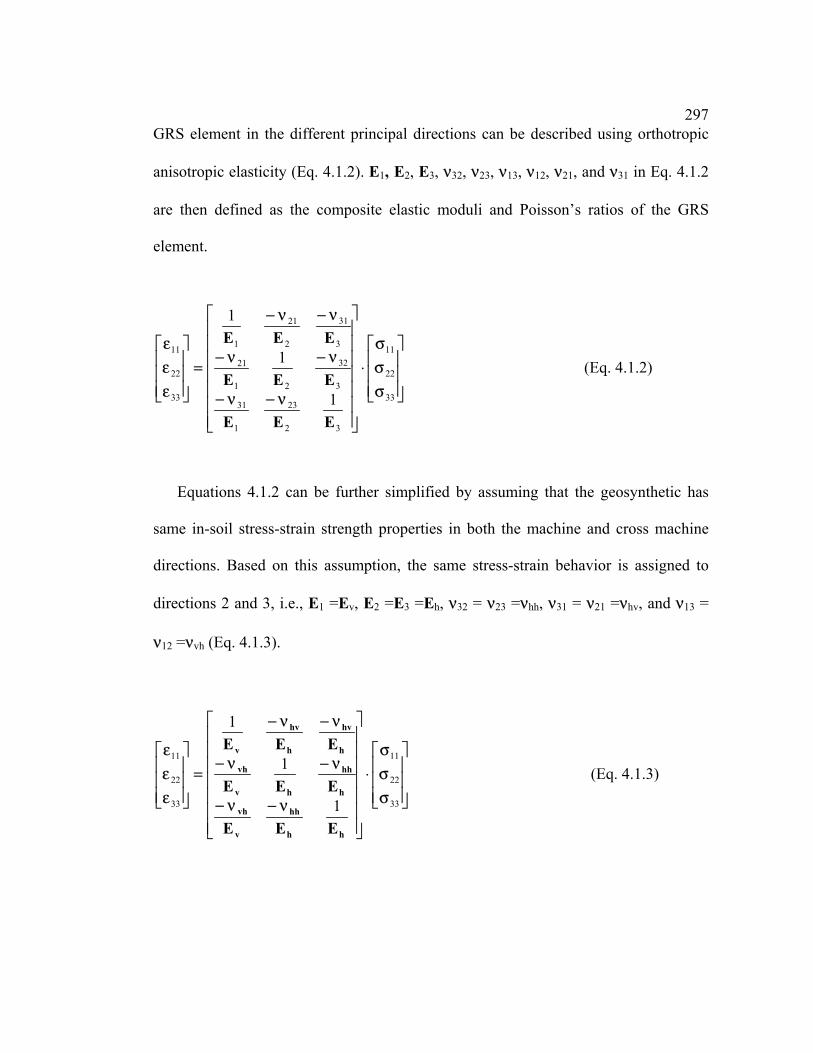
297GRS element in the different principal directions can be described using orthotropic
anisotropic elasticity (Eq. 4.1.2). E1, E2, E3, ν32, ν23, ν13, ν12, ν21, and ν31 in Eq. 4.1.2
are then defined as the composite elastic moduli and Poisson’s ratios of the GRS
element.
σσσ
⋅
ν−ν−
ν−ν−
ν−ν−
=
εεε
33
22
11
32
23
1
31
3
32
21
21
3
31
2
21
1
33
22
11
1
1
1
EEE
EEE
EEE
(Eq. 4.1.2)
Equations 4.1.2 can be further simplified by assuming that the geosynthetic has
same in-soil stress-strain strength properties in both the machine and cross machine
directions. Based on this assumption, the same stress-strain behavior is assigned to
directions 2 and 3, i.e., E1 =Ev, E2 =E3 =Eh, ν32 = ν23 =νhh, ν31 = ν21 =νhv, and ν13 =
ν12 =νvh (Eq. 4.1.3).
σσσ
⋅
ν−ν−
ν−ν−
ν−ν−
=
εεε
33
22
11
33
22
11
1
1
1
hh
hh
v
vh
h
hh
hv
vh
h
hv
h
hv
v
EEE
EEE
EEE
(Eq. 4.1.3)

298Moreover, for GRS elements inside a retaining structure, the plane strain loading
conditions are appropriate. In Figure 13.1.1, plane strain conditions indicate that there
is no strain in direction 2 (i.e. ε22 = γ12 = γ23 = 0 in Eq. 4.1.3). Equations 4.1.4 and 4.1.5
can then be used to describe the transversely isotropic elastic behavior of a GRS
element under plane strain loading conditions. Composite moduli of the GRS element
can be solved using this model with adequate material testing data, e.g., from the plane
strain test results.
hhh
hvvh EEE
33221122 0
σν−
σ+
σν−==ε (Eq. 4.1.4)
σσ
⋅
ν−
νν−ν−
νν−ν−
ν−
=
εε
33
112
2
33
11
1
1
h
hh
hh
hhhvhv
h
hhhvhv
h
hv
v
EEE
EEE (Eq. 4.1.5)
13.2 Interpreting UCD Test Results Using the Tranversely Isotropic Elasticity
Model
The UCD was designed to test a GRS element under plane strain loading conditions to
simulate the GRS element inside GRS soil structures (Boyle, 1995). The UCD
specimen is exactly a GRS element shown in Figure 13.1.1 with plane strain loading
conditions. Therefore, the developed transversely isotropic elasticity model can be
applied to interpret the UCD test results.

299
Equations 13.2.1 to 13.2.3 were rearranged from Equations 4.1.4 and 4.1.5.
11
3322
σσν−σ
=ν hhhv (Eq. 13.2.1)
( )[ ]331133
11 σ−+σ⋅ε
= CBEh (Eq. 13.2.2)
331111
11
σ−σ+εσ⋅
=BAE
EEh
hv (Eq. 13.2.3)
Where A = νhv2
B = -νhv - νhvνhh
C = νhh2
Also νvh = νhv Ev/Eh.
The terms σ11, σ22, σ33, ε11, and ε33 in Equations 13.2.1 to 13.2.3 were obtained by
reducing the UCD test data. However, there are still three unknowns (Ev, Eh, νhh, and
νhv) remaining in Equations 13.2.1 to 13.2.3, so numerical analysis was performed to
solve these equations. The steps of the numerical analysis were:
1. Formulate a spreadsheet using Equations 13.2.1 to 13.2.3,
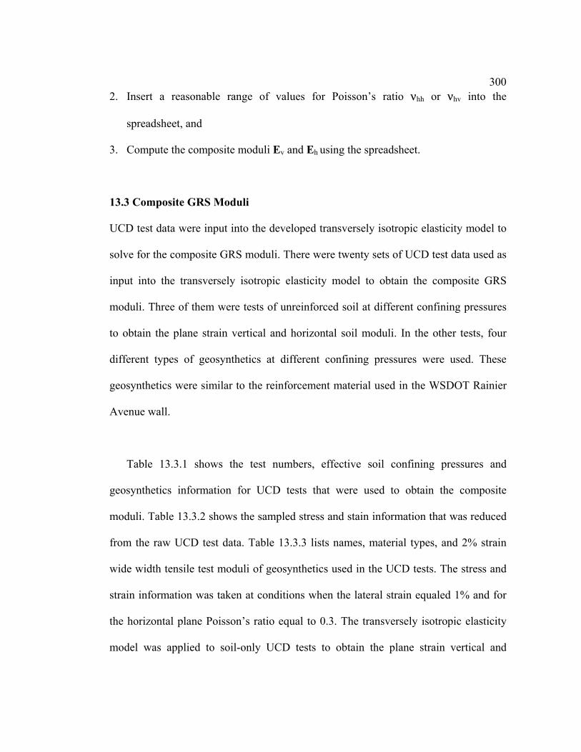
3002. Insert a reasonable range of values for Poisson’s ratio νhh or νhv into the
spreadsheet, and
3. Compute the composite moduli Ev and Eh using the spreadsheet.
13.3 Composite GRS Moduli
UCD test data were input into the developed transversely isotropic elasticity model to
solve for the composite GRS moduli. There were twenty sets of UCD test data used as
input into the transversely isotropic elasticity model to obtain the composite GRS
moduli. Three of them were tests of unreinforced soil at different confining pressures
to obtain the plane strain vertical and horizontal soil moduli. In the other tests, four
different types of geosynthetics at different confining pressures were used. These
geosynthetics were similar to the reinforcement material used in the WSDOT Rainier
Avenue wall.
Table 13.3.1 shows the test numbers, effective soil confining pressures and
geosynthetics information for UCD tests that were used to obtain the composite
moduli. Table 13.3.2 shows the sampled stress and stain information that was reduced
from the raw UCD test data. Table 13.3.3 lists names, material types, and 2% strain
wide width tensile test moduli of geosynthetics used in the UCD tests. The stress and
strain information was taken at conditions when the lateral strain equaled 1% and for
the horizontal plane Poisson’s ratio equal to 0.3. The transversely isotropic elasticity
model was applied to soil-only UCD tests to obtain the plane strain vertical and

301
Table 13.3.1 General Information of UCD Tests
UCD Test No. (Boyle, 1995)
Effective Soil Confining Pressure (kPa)
Geosynthetic Information (Name, 2% Mwwt1 (kN/m), material type)
115 12.4 Soil only
79 12.3 GTF 200, 103, polypropylene
77 10.4 GTF 375, 204, polypropylene
76 11.2 GTF 500, 357, polypropylene
98 10.6 GTF 1225T, 1126, polyester
112 24.6 Soil only
65 23.9 GTF 200, 103, polypropylene
67 23.3 GTF 200, 103, polypropylene
74 23.5 GTF 200, 103, polypropylene
81 23.1 GTF 200, 103, polypropylene
70 21.7 GTF 375, 204, polypropylene
73 22.0 GTF 375, 204, polypropylene
71 19.3 GTF 500, 357, polypropylene
99 22.5 GTF 1225T, 1126, polyester
100 25.0 GTF 1225T, 1126, polyester
111 21.3 GTF 1225T, 1126, polyester
54 47.6 Soil only
62 47.5 GTF 200, 103, polypropylene
55 43.6 GTF 375, 204, polypropylene
106 47.3 GTF 1225T, 1126, polyester 1 Wide Width Tensile test modulus (ASTM D 4595).

302Table 13.3.2 Sampled Stress-Strain Information from UCD tests
UCD Test No. (Boyle, 1995)
Vertical Strain (%)
Horizontal Strain (%)
Vertical Stress (kPa)
Lateral Stress1 (kPa)
Effective GRS Composite Lateral
Stress2 (kPa)
115 0.63 0.52 88.6 80.2 12.4
79 0.92 1.04 248.5 241.8 20.7
77 1.28 1.00 312.9 303.9 26.4
76 1.42 1.00 376.4 368.3 32.0
98 1.26 1.00 498.5 489.4 61.5
112 0.49 1.00 217.8 197.9 24.6
65 1.09 1.00 345.9 326.1 32.9
67 1.12 1.00 344.0 327.7 28.3
74 1.17 1.01 351.9 330.8 30.2
81 1.13 1.01 319.9 299.7 28.4
70 1.19 1.00 396.1 376.7 37.9
73 1.45 1.01 413.5 392.7 37.1
71 1.49 1.00 531.6 512.4 47.1
99 1.36 1.00 593.8 574.3 76.1
100 1.36 1.00 522.5 503.0 64.6
111 1.78 1.00 765.0 745.6 90.7
54 0.83 1.01 306.8 263.4 47.6
62 1.21 1.00 423.9 379.9 54.5
55 0.98 1.00 514.2 470.8 55.8
106 1.45 1.00 835.6 791.1 98.7 1 Lateral stress in the direction which there is no strain (plane strain controlled direction). 2 Calculated using the equation σ σ3comp ESCP
in soilTA
= + − (Boyle, 1995), where σ ESCP is
the effective soil confining pressure and A = effective lateral area of specimen.

303
Table 13.3.3 Geosynthetic material used in UCD tests (Boyle 1995)
Name Material Type 2% Mwwt1 (kN/m)
GTF 200 Polypropylene 103
GTF 375 Polypropylene 204
GTF 500 Polypropylene 357
GTF 1225 Polyester 1126 12% Mwwt = secant moduli from wide width tensile test at 2 % strain.
y = 75.514x + 7464.4R2 = 0.9886
y = 11215Ln(x) - 44382R2 = 0.9092
0.000E+00
1.000E+04
2.000E+04
3.000E+04
4.000E+04
5.000E+04
6.000E+04
0.0 100.0 200.0 300.0 400.0 500.0 600.0 700.0
Overburden Pressure (kPa)
Soil
Mod
ulus
(kPa
)
HorizontalVertical
Figure 13.3.1 Plane strain soil moduli obtained from UCD tests.

304horizontal soil moduli, in order to observe the reinforcing effect in both vertical
and horizontal direction.
Figure 13.3.1 shows the plane strain soil moduli results. Larger moduli were found
in the horizontal direction than in vertical direction because the UCD specimens were
compacted to the desired density during specimen preparation. Both horizontal and
vertical plane strain moduli increased as effective soil confining pressure increased.
The horizontal plane strain moduli increased linearly as effective soil confining
pressure increased; however, the vertical plane strain moduli increase was less at
higher effective soil confining pressures.
Figure 13.3.2 shows the results of horizontal GRS composite moduli versus the
effective soil confining pressure (ESCP), and Figure 13.3.3 shows the results of
vertical GRS composite moduli versus the ESCP. ESCP is the confining pressure that
is contributed by soil only; any confining pressure contributed by the tensile strength
of geosynthetic reinforcement was not considered. In UCD test data, ESCP is the
measured lateral soil pressure in direction 3, the direction that deformation was
allowed. As shown in Figures 13.3.2 and 13.3.3, both vertical and horizontal
composite moduli of GRS increased as the effective soil confining pressure increased
for a single geosynthetic reinforcement. For different geosynthetic reinforcements, the
tendency that composite moduli increased as the in-isolation tensile moduli of the
geosynthetic reinforcement increased was also observed. In both the horizontal and

305
0.000E+00
2.000E+04
4.000E+04
6.000E+04
8.000E+04
1.000E+05
1.200E+05
0.0 10.0 20.0 30.0 40.0 50.0 60.0
Effective Soil Confining Presure (kPa)
Hor
izon
tal C
ompo
site
Mod
ulus
(kPa
) GTF200GTF375GTF500GTF1225T
Figure 13.3.2 Horizontal composite moduli of GRS at 1% horizontal strain and with νhh=0.3.
0.000E+00
2.000E+04
4.000E+04
6.000E+04
8.000E+04
1.000E+05
1.200E+05
0.0 10.0 20.0 30.0 40.0 50.0 60.0
Effective Soil Confining Presure (kPa)
Verti
cal C
ompo
site
Mod
ulus
(kPa
)
GTF200GTF375GTF500GTF1225T
Figure 13.3.3 Vertical composite moduli of GRS at 1% horizontal strain and with
νhh=0.3.
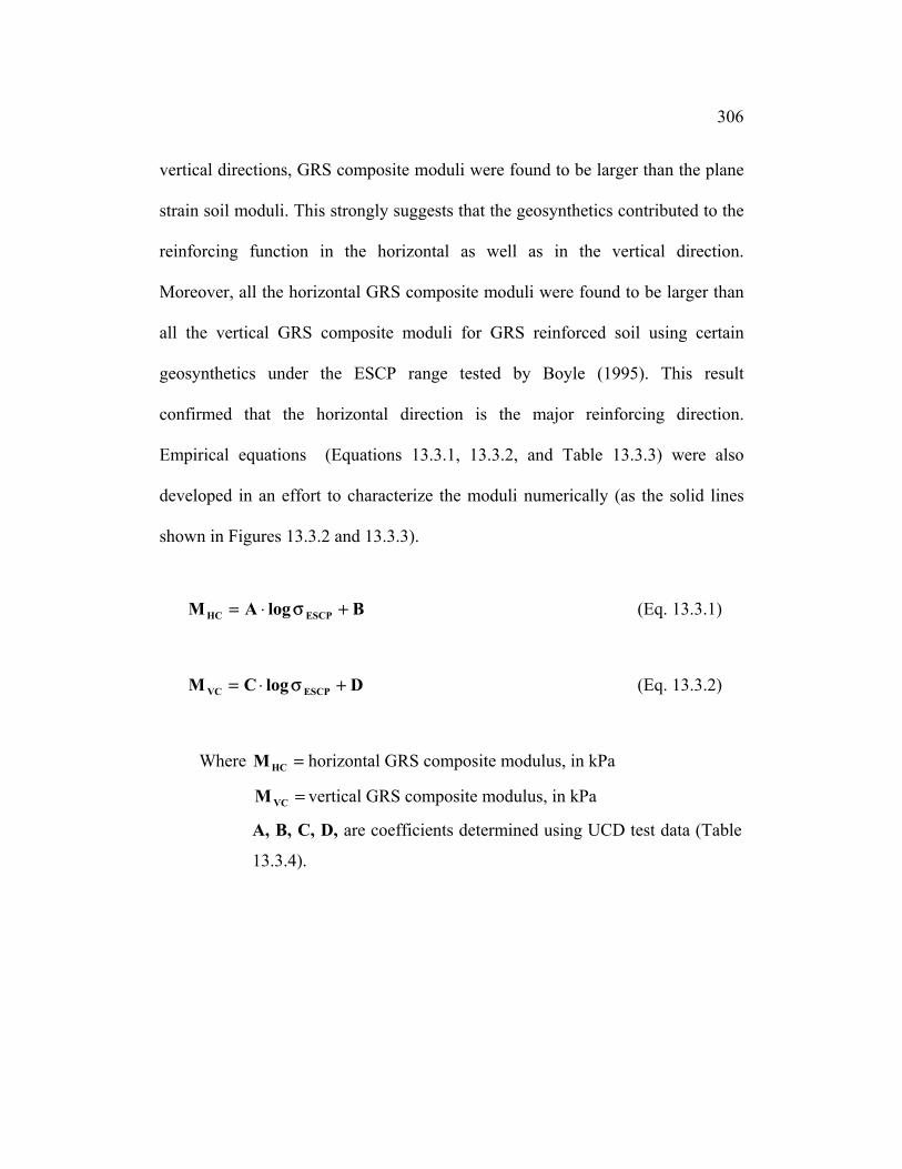
306
vertical directions, GRS composite moduli were found to be larger than the plane
strain soil moduli. This strongly suggests that the geosynthetics contributed to the
reinforcing function in the horizontal as well as in the vertical direction.
Moreover, all the horizontal GRS composite moduli were found to be larger than
all the vertical GRS composite moduli for GRS reinforced soil using certain
geosynthetics under the ESCP range tested by Boyle (1995). This result
confirmed that the horizontal direction is the major reinforcing direction.
Empirical equations (Equations 13.3.1, 13.3.2, and Table 13.3.3) were also
developed in an effort to characterize the moduli numerically (as the solid lines
shown in Figures 13.3.2 and 13.3.3).
M A BHC ESCP= ⋅ +log σ (Eq. 13.3.1)
M C DVC ESCP= ⋅ +log σ (Eq. 13.3.2)
Where M HC = horizontal GRS composite modulus, in kPa
M VC = vertical GRS composite modulus, in kPa
A, B, C, D, are coefficients determined using UCD test data (Table
13.3.4).
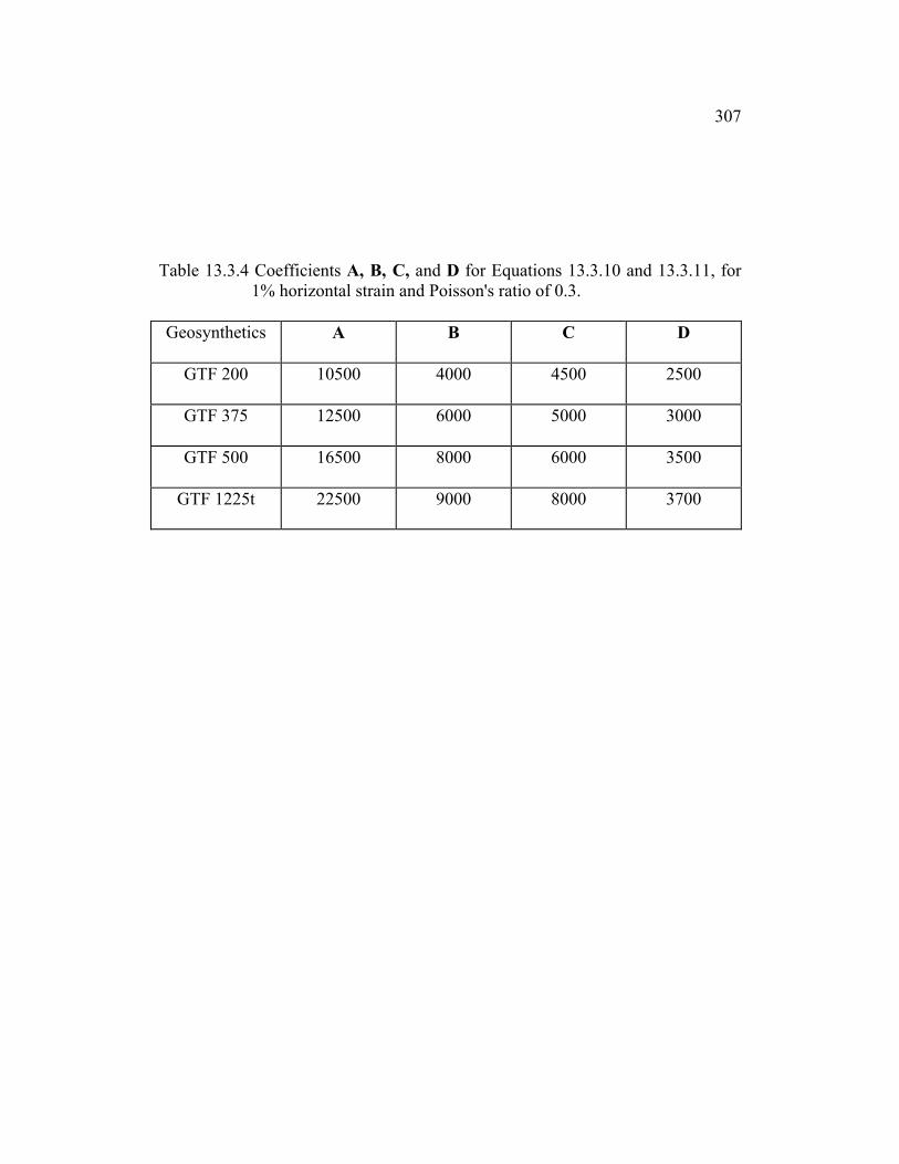
307
Table 13.3.4 Coefficients A, B, C, and D for Equations 13.3.10 and 13.3.11, for
1% horizontal strain and Poisson's ratio of 0.3. Geosynthetics A B C D
GTF 200 10500 4000 4500 2500
GTF 375 12500 6000 5000 3000
GTF 500 16500 8000 6000 3500
GTF 1225t 22500 9000 8000 3700
308
13.4 Numerical Models Using Composite GRS Properties
Two FLAC models (Models COMPA and COMPS) were created in order to
verify the developed composite approach. GRS moduli obtained using the
developed analytical model were input into Models COMPA and COMPS to
simulate the performance of the WSDOT Rainier Avenue wall. Both Models
COMPA and COMPS are the composite property models that consist of only
anisotropic elastic material elements. Typical cross and instrumentation sections
of Rainier Avenue wall were shown in Figures 9.2.1 and 9.2.2. Input properties of
these anisotropic elastic material elements are the horizontal modulus, the vertical
modulus, and Poisson’s ratios in different principal directions. Model COMPA is
the model that simulates the Rainier Avenue wall performance at the end of
construction, and Model COMPS is the model that simulates the wall
performance after applying the surcharge. The GRS composite strength properties
obtained from transversely isotropic elasticity are used as the input properties for
both models COMPA and COMPS.
Figures 13.4.1 and 13.4.2 show the results of the numerical analysis at 3m
behind the wall. Inclinometer measurements at the same location as well as the
result of Model 5008P (the discrete element model) were also plotted. Successful
simulation results were obtained from both models COMPA and COMPS. The
deflection results of both models COMPA and COMPS show good agreements
with inclinometer measurements, both at the end of construction and after

309
Figure 13.4.1 Results of deflections of Models COMPA and 5008P at 3m behind
wall face.
Figure 13.4.2 Results of deflections of Models COMPS and 5008P at 3m behind wall face.
19.75
21.75
23.75
25.75
27.75
29.75
31.75
33.75
0 20 40 60 80 100
Inclinometer Delfection (mm)
Elev
atio
n (m
)
Model COMPAInclinometer DeflectionModel 5008P
19.75
21.75
23.75
25.75
27.75
29.75
31.75
33.75
0 20 40 60 80 100 120
Inclinometer Delfection (mm)
Elev
atio
n (m
)
Model COMPSInclinometer DeflectionModel 5008p2

310
Table 13.4.1 Measurements of strain gages and extensometers inside Rainier
Avenue wall at locations 3m behind wall face (after Allen et al., 1992).
Elevations (m) End of Construction After Surcharge
SG (%) ES (%) SG (%) ES (%)
21.27 0.25 -- 0.31 --
23.17 0.4 0.45 0.6 0.6
26.21 0.9 -- 1.2 --
29.63 0.8 -- 1.4 --
SG: strain gage measurements. ES: extensometer measurement.

311
surcharge was applied. As shown in Figure 13.4.1, model COMPA was able to
predict the wall deflection at the upper half of the wall. It tended to overestimate
the deflection at the lower half of the wall by an average of about 10mm. This
result indicated that the wall had horizontal strains less than 1% below elevation
25.75m and close to 1% above this elevation because the input composite GRS
moduli were sampled at 1% horizontal strain. This agreement of horizontal strains
has been verified with strain measurements listed in Table 13.4.1.
Similar modeling results were also found in model COMPS. Figure 13.4.2
shows that Model COMPS tended to overestimate the deflection at the lower
portion of the wall and underestimate the deflections at the upper portion of the
wall. This result also verified the observation that the Rainier Avenue wall had
horizontal strains less than 1% below elevation 25m and larger than 1% above
this elevation (Figure 13.4.2). Measurements of strain gages and extensometers
listed in Table 13.4.1 show that the Rainier Avenue wall had horizontal strains
close to 1% at the end of construction and larger than 1% after surcharge at upper
portion of the wall.

312
13.5 Conclusions
1. Feasibility of analyzing GRS composite properties using the developed
transversely isotropic elasticity model has been demonstrated.
2. Different composite moduli of GRS elements were found in different
principal directions using the transversely isotropic elasticity model; the
assumption that different reinforcing mechanisms existing in different
principal directions inside a GRS is further verified.
3. Because the input GRS composite properties were sampled at an average
working strain of the Rainier Avenue wall (1%), numerical models COMPA
and COMPS were able to predict quite well the field instrumentation
measurements. To improve this approach so that it can be more universally
applicable, the developed transversely isotropic elasticity model for GRS
elements should be applied to additional UCD test results. The behavior of
GRS composites sampled at different horizontal strains, for example, 0.5%,
1.5%, and 2%, should be analyzed. The stress-strain distribution of GRS
retaining structures can then be further analyzed using composite property
models with input of moduli sampled at these horizontal strains.

313Chapter 14
Applications of Modeling Results: Performance Prediction and
Design Recommendations for GRS Walls
In this chapter, methods of predicting GRS wall performance factors such as
maximum face deflection and maximum reinforcement tension, as well as design
recommendations for GRS walls are presented. The performance prediction methods
were developed based on the results of the parametric study presented in Chapter 12.
They were developed in an effort to provide preliminary working stress information
for the initial designs of GRS walls. General conditions of using these methods to
predict GRS wall performance are as same as the boundary conditions and design
factors described in Section 12.4.1. These performance prediction methods include (1)
a maximum face deflection prediction method (Section 14.1), (2) a maximum
reinforcement tension prediction method (Section 14.2), and (3) a new method for
predicting reinforcement tension distributions (Section 14.3). In the example problems
that used the developed method to predict the GRS wall performance, verification was
provided by the instrumentation measurements of the Algonquin concrete panel faced
geogrid wall (Wall 2). Limitations of the prediction method are discussed in Section
14.4. Finally, design recommendations for GRS walls are presented in Section 14.5.
These recommendations are based on the results of the case history modeling
(Chapters 9 and 10) and the parametric study (Chapter 12).

31414.1 Maximum Face Deflection
Figure 14.1.1 presents a simplified method to predict the maximum face deflection of
GRS walls. Design curves shown in Figure 14.1.1 are the trend lines of the parametric
study results shown in Figure 12.8.1. In Figure 14.1.1, GRS walls were categorized
into three groups: (I) large spacing with a wrapped face, (II) large spacing with a
structural facing or small spacing with a wrapped face, and (III) small spacing with a
structural facing. These three curves were the trend lines of the modeling results of
GRS walls that were designed with Type II (φ = 30 deg) to Type VII (φ = 55 deg) soils
(Table 12.4.2) and global reinforcement stiffnesses between 500 to 5500 kN/m2. They
can be used to predict the face deflection if the material properties are given, or to
estimate required reinforcement stiffness if the soil properties and tolerable
deformation are given. Examples 14.1.1 and 14.1.2 show the sample calculations for
utilizing Figure 14.1.1.
14.2 Reinforcement Tension
Maximum reinforcement tensions can be estimated using the analytical model
presented in Chapter 11. Equation 11.1.6 is the expression for the accumulated
reinforcement tension at a given depth from top of the wall. The reinforcement tension
of an individual reinforcement layer (Equation 14.2.2) can be obtained by subtracting
Equation 14.2.1 (the accumulated reinforcement tension of layer n-1) from Equation
11.1.6.
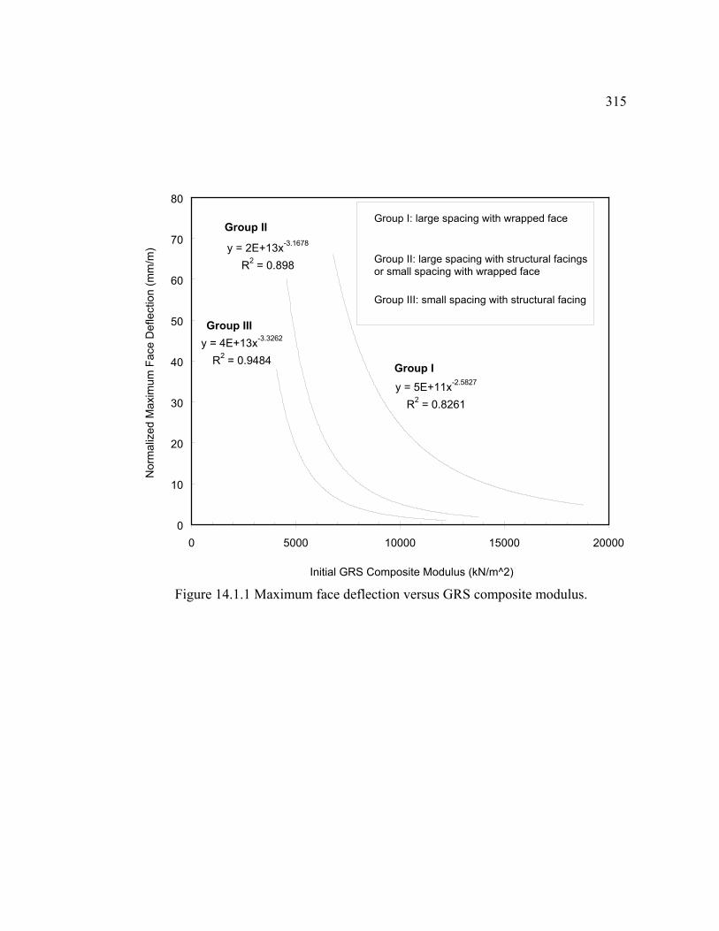
315
Figure 14.1.1 Maximum face deflection versus GRS composite modulus.
y = 2E+13x-3.1678
R2 = 0.898
y = 5E+11x-2.5827
R2 = 0.8261
y = 4E+13x-3.3262
R2 = 0.9484
0
10
20
30
40
50
60
70
80
0 5000 10000 15000 20000
Initial GRS Composite Modulus (kN/m^2)
Nor
mal
ized
Max
imum
Fac
e D
efle
ctio
n (m
m/m
)
Group I: large spacing with wrapped face
Group II: large spacing with structural facingsor small spacing with wrapped face
Group III: small spacing with structural facing
Group I
Group II
Group III

316Example 14.1.1 Maximum face deflection prediction.
******************************************************************
Given: 1. Wall height (H) = 6m, reinforcement spacing (Sv) = 0.8m, vertical face.
2. Backfill soil properties: γ = 20.6 kN/m3, φ = 45 deg, angular sand.
3. Reinforcement stiffness (J): 1000 kN/m (after in-soil and low strain rate
modifications).
Solve:
Calculating the initial GRS composite modulus using Equation 11.2.7,
sv
comp ESJE += (Eq. 11.2.7)
where 2v m
kN12508.0
1000SJ ⋅== , and calculating Es using Equation
7.1.3 with Rf = 0.7, n = 0.5, K = 1600 (Table 12.4.2), and
2S
K v03 ⋅γ⋅=σ = 2.42 kPa, where K0 = 1-sinφ.
( )( ) n
atm
3atm
2
3
31fs P
PKsin2cosc2
sin1R1E
σ⋅⋅⋅
φ⋅σ+φ⋅
σ−σφ−−= = 10,088 kN/m2
Ecomp = 1250 + 10088 = 11,338 kN/m2
Sv = 0.8m → large spacing
Wall Types
Dmax/H (mm/m)
dmax (mm)
Measured Face Deflection (mm)a
Wrapped face, Group I curve 17 102 --
Structural facing, Group II curve 5 30 32 a Measured maximum face deflection of Algonquin concrete panel
face wall (J = 1020 kN/m, Sv = 0.76m, similar soil properties as given above)
******************************************************************

317Example 14.1.2 Calculating required reinforcement stiffness.
******************************************************************
Given: 1. Wall height (H) = 10m, reinforcement spacing (Sv) = 0.4m, vertical face.
2. Backfill soil properties: γ = 20.6 kN/m3, φ = 45 deg, angular sand.
3. Tolerable maximum face deflections: 75 and 100mm for wrapped face
walls, 25 and 50 mm for structural facing walls.
Solve:
Es = 7133 kN/m2 (as calculated in Example 14.1.1)
Dmax
(mm)
dmax/H
(mm/m)
Ecomp
(kN/m2)
J/Sv = Ecomp - Es
(kN/m2)
J
(kN/m2)
75 7.5 9000 1867 747
100 10 8000 867 347
25 2.5 9000 1867 747
50 5 7500 367 147
******************************************************************

318
)KK(2z
)z(t compsoil
2n
n
1i −⋅
⋅γ=∑ (Eq. 11.1.6)
)KK(2z
)z(t compsoil
21n
1n
1i −⋅
⋅γ= −
−
∑ (Eq. 14.2.1)
)zz()KK(2
ttt 21n
2ncompsoil
1n
1i
n
1in −
−
−⋅−⋅γ=−= ∑∑ (Eq. 14.2.2)
Equation 14.2.2 can be rearranged as Equation 14.2.3, where zn - zn-1 = Sv, the
reinforcement spacing, and n1nn z
2)zz(
≈+ − . Reinforcement tension at a given layer
can then be expressed in terms of Sv and zn (Equation 14.2.4).
)zz()zz()KK(2
t 1nn1nncompsoiln −− +⋅−⋅−⋅γ= (Eq. 14.2.3)
nvcompsoiln zS)KK(t ⋅⋅γ⋅−≈ (Eq. 14.2.4)
The maximum reinforcement tension can be expressed using Equation 14.2.5:
vmaxtcompsoilmax Sz)KK(T ⋅⋅γ⋅−=
vmaxtcompsoil SH
Hz)KK(
⋅⋅γ⋅⋅−
= (Eq. 14.2.5)
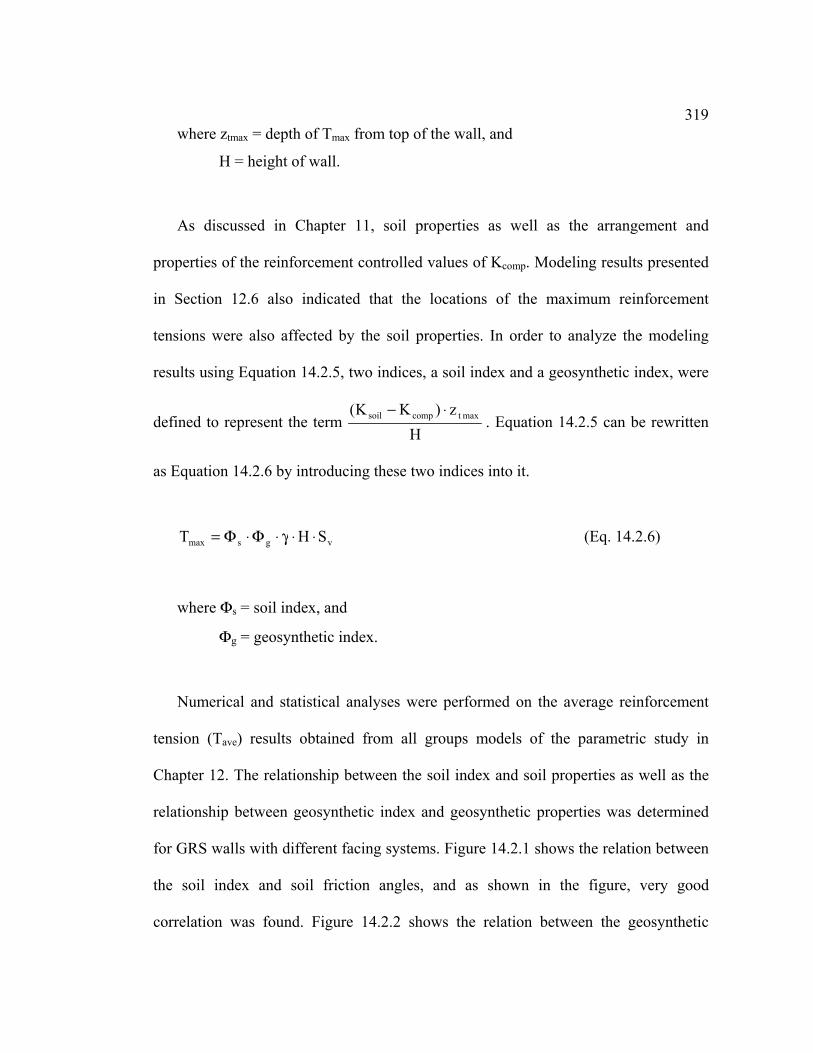
319where ztmax = depth of Tmax from top of the wall, and
H = height of wall.
As discussed in Chapter 11, soil properties as well as the arrangement and
properties of the reinforcement controlled values of Kcomp. Modeling results presented
in Section 12.6 also indicated that the locations of the maximum reinforcement
tensions were also affected by the soil properties. In order to analyze the modeling
results using Equation 14.2.5, two indices, a soil index and a geosynthetic index, were
defined to represent the term H
z)KK( maxtcompsoil ⋅−. Equation 14.2.5 can be rewritten
as Equation 14.2.6 by introducing these two indices into it.
vgsmax SHT ⋅⋅γ⋅Φ⋅Φ= (Eq. 14.2.6)
where Φs = soil index, and
Φg = geosynthetic index.
Numerical and statistical analyses were performed on the average reinforcement
tension (Tave) results obtained from all groups models of the parametric study in
Chapter 12. The relationship between the soil index and soil properties as well as the
relationship between geosynthetic index and geosynthetic properties was determined
for GRS walls with different facing systems. Figure 14.2.1 shows the relation between
the soil index and soil friction angles, and as shown in the figure, very good
correlation was found. Figure 14.2.2 shows the relation between the geosynthetic

320index and the global reinforcement stiffnesses that were corrected with considerations
of in-soil and low strain rate effects. As shown in the figure, very good correlation was
also found in this case for all models; however the geosynthetic indexes were not
affected very much by the facing systems (Figure 14.2.2).
Magnitudes of the maximum average reinforcement tensions (Tave_max) can be
estimated using Equation 14.2.6. The soil and geosynthetic indices in Equation 14.2.6
can be determined using Figures 14.2.1 and 14.2.2. Design curves shown in Figures
14.2.3 and 14.2.4 are the trend lines of the modeling results shown in Figures 14.2.1
and 14.2.2. Table 14.2.1 shows the average ratios (aT) of the maximum average
reinforcement tension to the maximum peak reinforcement tension (Tpeak_max / Tave_max)
of all models analyzed in this study. The maximum peak reinforcement tensions
(Tpeak) obtained from the numerical models tended to over-predict the actual peak
reinforcement tensions in the GRS walls because the reinforcement elements were
attached to the material element nodes. Details of this over-estimation were described
in Section 8.5.6. From field measurements of case histories analyzed in this research,
Tpeak obtained from the numerical models with reinforcement elements attached to the
nodes tended to over-predict the actual peak reinforcement tension by about 20%.

321
Figure 14.2.1 Soil index of walls with different facing systems.
Figure 14.2.2 Geosynthetic index of walls with different facing systems.
y = 136.11x-1.9985
R2 = 0.9684
y = 69.071x-1.9345
R2 = 0.9235
0
0.1
0.2
0.3
20 25 30 35 40 45 50 55 60
Soil Friction Angle (deg)
Soil
Inde
x
Wrapped face
Secondary reinforcement
Structural facing
y = 0.3129x0.1633
R2 = 0.9573
0.6
0.8
1
1.2
1.4
1.6
0 2000 4000 6000 8000 10000 12000
Corrected Global Reinforcement Stiffness (kN/m^2)
Geo
synt
hetic
Inde
x
Wrapped face
Secondary reinforcement
Structural facing, large spacing
Structural facing, small spacing

322
Figure 14.2.3 Design curves of soil index.
Figure 14.2.4 Design curve of geosynthetic index.
y = 0.3035x0.1678
R2 = 0.9397
0.6
0.8
1
1.2
1.4
1.6
0 2000 4000 6000 8000 10000 12000
Corrected Global Reinforcement Stiffness (kN/m^2)
Geo
synt
hetic
Inde
x
y = 136.11x-1.9985
R2 = 0.9684
y = 69.071x-1.9345
R2 = 0.9235
0
0.1
0.2
0.3
20 25 30 35 40 45 50 55 60
Soil Friction Angle (deg)
Soil
Inde
xWrapped face
Structural face

323Maximum peak reinforcement tensions can be estimated using aT and Equation
14.2.6 (Equation 14.2.7).
vgsTmax_aveTmax_peak SHaTaT ⋅⋅γ⋅Φ⋅Φ⋅=⋅= (Eq. 14.2.7)
where aT = ratio of (Tpeak_max / Tave_max) (Table 14.2.1),
Φs = soil index, and
Φg = geosynthetic index.
Example 14.2.1 shows the sample calculation for determining the maximum
reinforcement tensions using Equations 14.2.6 and 14.2.7 and design curves shown in
Figures 14.2.3 and 14.2.4. In Example 14.2.1, maximum reinforcement strain of the
given GRS wall is determined as 0.86%. The maximum reinforcement strain measured
in Algonquin concrete panel Wall 2 (geogrid wall), which had similar material
properties and geometry design as given in the example, was 0.8%.

324
Table 14.2.1 Values of aT for different GRS walls.
Wall Types aT
Wrapped face, large spacing (Sv = 0.76m) 1.8
Wrapped face, small spacing (Sv = 0.38m) 1.5
Wrapped face, with secondary reinforcement, large spacing 1.7
Modular block face, large spacing 1.7
Modular block face, small spacing 1.5
Concrete panel face, large spacing 2.2
Concrete panel face, small spacing 1.8

325Example 14.2.1 Maximum reinforcement tensions prediction.
****************************************************************** Given: 1. Wall height (H) = 6m, reinforcement spacing (Sv) = 0.75 m,
vertical face.
2. Backfill soil properties: γ = 20.6 kN/m3, φ = 43 deg, angular sand.
3. Reinforcement stiffness (J): 1000 kN/m (after in-soil and low strain
rate modifications).
Solve:
Φs = 0.09 (wrapped face) and 0.05 (structural face) for φ = 43 deg
Φg = 1.05 for 2v m
kN133375.0
1000SJ ⋅==
vgsmax_ave SHT ⋅⋅γ⋅Φ⋅Φ= (Eq. 14.2.6)
Tpeak_max = aT Tave_max (Eq. 14.2.7)
where γ = 20.6 kN/m3, H = 6m, and Sv = 0.75m.
Wall Types
Tave_max, (kN/m)
(Eq.14.2.6)
Tpeak_max, (kN/m)
(Eq. 14.2.7)
Corrected Tmax
(kN/m)a
Tmax (kN/m) (Tie-back wedge
method)b
Wrapped Face 8.8 15.8 12.6 17.6
Modular Face 4.9 8.3 6.6 17.6
Concrete Face 4.9 10.8 8.6 17.6 a Apply 20% reduction on Tpeak_max obtained using Equation 14.2.7 (Section 8.5.6). b Tmax = KaγHSv, where Ka is the active lateral earth pressure coefficient,
Ka = 0.19 for φ = 43 deg.
Maximum reinforcement strains can be also obtained by dividing the Tpeak_max by the reinforcement stiffness:
Wrapped Face Wall
Modular Block Faced Wall
Concrete Panel Faced Wall
Maximum Reinforcement Strain (%)
1.26
0.66
0.86
******************************************************************

32614.3 Reinforcement Tension Distributions
Results of case histories, laboratory test walls, and parametric study indicated that the
actual reinforcement tension distributions inside the GRS walls were very different
from the reinforcement tension distributions calculated using the tie-back wedge
method. Results of the parametric analysis indicated that locations of the maximum
reinforcement tensions occurred between 0.25H (poor quality backfill) to 0.5H (good
quality backfill). The tie-back wedge method predicts a maximum reinforcement
tension at the bottom of the wall. Moreover, modeling results presented in Chapter 9
also showed that the actual reinforcement tensions inside the GRS walls were smaller
than the maximum reinforcement tensions predicted using the tie-back wedge method.
Figure 14.3.1 shows a trapezoid reinforcement tension distribution for GRS walls.
This distribution was developed in order to cover all the reinforcement tension
distributions that were observed in the field measurements (Chapter 9) and parametric
study (Chapter 12). As shown in Figure 14.3.1, reinforcement tension increases from
0.2 Tmax at top of the wall to the maximum reinforcement tension (Tmax) at height
equal to 0.6H. The reinforcement tension remains at Tmax between 0.6H to 0.2H, and it
decreases from Tmax to 0.2 Tmax at bottom of the wall.

327
Figure 14.3.1 Reinforcement tension distribution of GRS walls.
0
0.1
0.2
0.3
0.4
0.5
0.6
0.7
0.8
0.9
1
0 0.2 0.4 0.6 0.8 1 1.2
Normalized Reinforcement Tension (T/Tmax)
Nor
mal
ized
Hei
ght (
h/H
)

328Tmax can be determined using Equations 14.2.6 and 12.4.7 and design curves
shown in Figures 14.2.3 and 14.2.4 with modification to account for the over-
prediction caused by attaching reinforcement elements to the material element nodes.
Example 14.3.1 shows the procedures to determine the reinforcement tension
distribution inside a GRS wall. Figure 14.3.2 shows the reinforcement tension
distribution calculated in Example 14.3.1 compared to the tension distribution
converted from the strain gage measurements (Algonquin concrete panel Wall 2).
Excellent prediction was obtained by using the method presented in this chapter.
14.4 Limitations of the Performance Prediction Methods
Performance prediction methods presented in this chapter were developed based on
the result of the extensive parametric study performed in this research (Chapter 12).
Limitations of using these methods to predict performance of the GRS walls include
the general boundary conditions, the ranges of the design factors, and geometry limits
that are similar to those in the numerical models of the parametric study. Details of
these limitations are described in the following sections.
14.4.1 Wall Geometry
Numerical GRS wall models analyzed in the parametric study have heights ranging
from 12.6 m to 3.6 m., and all the models were designed with vertical faces. For GRS
walls that are higher than 12.6 m, performance prediction made by the design curves
presented in this chapter may not be reliable.

329
By comparing the analysis results of the parametric models and case histories
presented in Chapter 9, both wall face deflections and reinforcement tensions of a
battered face wall were found to be smaller than vertical face walls with the same
backfill soil properties and reinforcement layout and properties. Therefore, design
curves presented in this chapter tend to over-predict the performance of GRS walls
with battered faces.
14.4.2 Boundary Conditions
For all models analyzed in the parametric study, the backfill was extended backward a
distance equal to the embeded reinforcement length from the end of the reinforcement.
The foundation soil in front of the wall was also extended a distance equal to the
embedded reinforcement length from the toe of the wall. The depth of foundation soil
was equal to the height of the wall. For GRS walls that have boundary conditions
extending further than those described above, design curves presented in this chapter
can be used to predict their performance. However, for GRS walls that have more
complicated boundary conditions, such as GRS walls on a bedrock foundation or that
have bedrock next to the reinforced zone, design curves presented in this chapter
might not be appropriate.
These design curves were developed based on the results of numerical models that
have no foundation failure and no embedment or constraint at the toe. Use of these

330design curves is also limited to GRS wall cases without foundation soil failure and
with free toe restraint.
14.4.3 Soil Properties
Design curves presented in this chapter were developed based on the results of the
numerical models with backfill of Soil Type II to VII (Table 12.4.2). Therefore, these
design curves are appropriate for predicting performance of GRS walls with backfill
soil properties similar to Soil Type II to VII as listed in Table 12.4.2.
14.4.4 Reinforcement Properties and Arrangement
Design curves presented in this chapter were developed based on the results of the
numerical models with reinforcement stiffness (global) ranging from 100 kN/m2 to
5,000 kN/m2. Moreover, the vertical spacing used in the parametric study ranged from
0.38 m to 0.76 m, and embedment length of the reinforcement was fixed to 80% of the
wall height for all models. For GRS walls with reinforcement properties and
arrangement other than those conditions described above, design curves presented in
this chapter are not suitable for predicting their performance.

331Example 14.3.1 Prediction of the reinforcement tension distribution.
******************************************************************
Given: 1. Wall height (H) = 6m, reinforcement spacing (Sv) = 0.75m,
vertical concrete panel face.
2. Backfill soil properties: γ = 20.6 kN/m3, φ = 43 deg, angular sand.
3. Reinforcement stiffness (J): 1000 kN/m (after in-soil and low strain
rate modifications).
Solve:
Tmax = 8.6 kN/m (Example 14.2.1)
Reinforcement Layer
h/H
Reinforcement Tension,
(Tmax)
Reinforcement Tension, (kN/m)
1 0.000 0.20 1.7
2 0.063 0.45 3.9
3 0.188 0.95 8.2
4 0.313 1.00 8.6
5 0.438 1.00 8.6
6 0.563 1.00 8.6
7 0.688 0.82 7.1
8 0.813 0.57 4.9

332
Figure 14.3.2 Predicted and measured reinforcement distribution of Algonquin
concrete panel faced geogrid wall.
0.0
0.2
0.4
0.6
0.8
1.0
0 2 4 6 8 10 12 14 16 18 20Reinforcement Tension (kN/m)
Nor
mal
ized
Hei
ght (
h/H
)
Predicted using Equations 14.2.6and 14.2.7
Measured (calculated using straingage measurements)
Predicted using tie-back wedgemethod

33314.5 Design Recommendations for GRS Walls
1. Results of the parametric study indicate that the reinforcement lengths equal to
0.8H (H is the height of the wall) seems to be adequate. Even models designed
with very poor quality backfill material (φ = 25 deg) or very weak reinforcement (J
= 55 kN/m) showed no failures in the backfill behind the reinforced zone. Only
localized failures were found at the face of wrapped walls with large spacing.
2. Reinforcement spacings larger than 0.6m are not recommended for use in the
wrapped face wall design. Local failures were observed in the results of the
wrapped face wall models with spacings larger than 0.6m. Face deflection profiles
and reinforcement tension distributions of these large spacing wrapped face wall
models shown in Chapter 12 also indicated that these local failures can cause
internal instability such as outward rotation of the wall face.
3. Material properties such as plane strain soil properties and in-soil low strain rate
reinforcement stiffnesses have to be carefully investigated when designing GRS
retaining structures. Modeling results shown in Chapters 9 and 10 indicated that
the performance of GRS walls can be accurately reproduced with correct material
property information. To investigate the material properties inside the GRS
retaining structures, property determination procedures presented in Chapter 7 can
be used as a guideline.
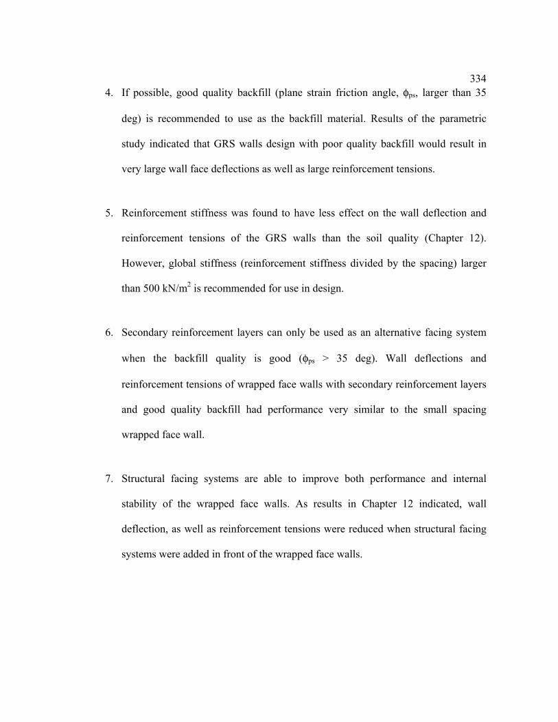
3344. If possible, good quality backfill (plane strain friction angle, φps, larger than 35
deg) is recommended to use as the backfill material. Results of the parametric
study indicated that GRS walls design with poor quality backfill would result in
very large wall face deflections as well as large reinforcement tensions.
5. Reinforcement stiffness was found to have less effect on the wall deflection and
reinforcement tensions of the GRS walls than the soil quality (Chapter 12).
However, global stiffness (reinforcement stiffness divided by the spacing) larger
than 500 kN/m2 is recommended for use in design.
6. Secondary reinforcement layers can only be used as an alternative facing system
when the backfill quality is good (φps > 35 deg). Wall deflections and
reinforcement tensions of wrapped face walls with secondary reinforcement layers
and good quality backfill had performance very similar to the small spacing
wrapped face wall.
7. Structural facing systems are able to improve both performance and internal
stability of the wrapped face walls. As results in Chapter 12 indicated, wall
deflection, as well as reinforcement tensions were reduced when structural facing
systems were added in front of the wrapped face walls.

3358. Preliminary design information such as maximum face deflection and
reinforcement tension distributions can be obtained by using the prediction
methods described in this chapter (Chapter 14).
9. With material properties and design geometry given, maximum face deflection of
GRS walls can be predicted using Figure 14.1.1 (see Example 14.1.1). The
maximum face deflection calculated in Example 14.1.1 showed an excellent
agreement to the field measurement of the wall that was the basis for this example.
Figure 14.1.1 can also be used to determine the required reinforcement stiffness if
soil properties and design geometry are given (Example 14.1.2).
10. Example 14.2.1 shows the procedures to determine the maximum reinforcement
tension inside the GRS walls using Equations 14.2.6 and 14.2.7 and design curves
shown in Figures 14.2.3 and 14.2.4. Maximum reinforcement tension that was
calculated in Example 14.2.1 was also found to be very close to the maximum
reinforcement tension reduced from the strain gage measurement on the real wall.
11. Figure 14.3.1 shows a reinforcement tension distribution that was developed based
on the working stress-strain information of an extensive parametric study. In this
figure, reinforcement tension increases from 0.2 Tmax at the top of the wall to the
maximum reinforcement tension (Tmax) at a height equal to 0.6H. The
reinforcement tension remains at Tmax between 0.6H to 0.2H, and it decreases from
Tmax to 0.2 Tmax at bottom of the wall. As shown in Example 14.3.1 and Figure

33614.3.2, the reinforcement tension distribution of the Algonquin concrete panel
faced Wall 2 was able to be accurately reproduced by using Figure 14.3.1.
12. For critical cases, an extensive numerical analysis is still recommended so that
complete working stress-strain information can be obtained for internal stability
analyses. Determination of material properties and modeling techniques as
described in Chapters 7 and 8 can be used as the “general rules” for performing the
numerical analyses.

337Chapter 15
Summary, Conclusions, and Recommendations for Future Research
15.1 Summary
The conventional internal stability design approach using limiting equilibrium is not
appropriate for internal stability analyses of GRS retaining structures. This is because
of the considerable differences of properties between the traditional steel and
geosynthetic reinforcement. Present GRS wall design methods such as the tie-back
wedge method tend to overestimate the internal stress levels inside the GRS walls,
especially in the lower half of the wall. Previous research on this subject has not made
much progress because:
1. Little information on the internal stress or strain distributions in real GRS
structures was available,
2. Numerical modeling techniques for analyzing the performance of GRS walls has
been problematic, and
3. Understanding of material and interface properties of GRS walls was not well
developed.
This research project was an effort to improve our understanding of the internal
stress-strain distribution in GRS retaining structures. The face deformations and
internal stress-strain distributions of GRS retaining structures were analyzed using
numerical techniques. Numerical models were first developed to simulate the field

338instrumentation measurements in real walls. The same modeling techniques were then
applied to develop numerical models for full scale test walls in order to predict their
performance. Parametric studies were also carried out to investigate the influence of
different internal stability design factors. Finally, improved techniques for analyzing
the face deformations and internal stress-strain distributions as well as an improved
internal stability design procedure were developed.
This research has contributed to progress in the following areas:
1. Better understanding of the material properties inside the GRS retaining
structures. Material properties such as plane strain soil properties and low
confining pressure soil dilation angle were carefully investigated in this
research (Chapter 7).
2. Modeling techniques for working stress analyses of GRS retaining structures.
Modeling techniques (Chapter 8) were developed in this research to reproduce
both the external and internal working stress information of the selected case
histories (Chapter 9), as well as to perform Class A predictions on the
performance of three well instrumented laboratory test walls (Chapter 10).
Results of these numerical modeling appeared to be successful.
3. Analytical models for analyzing the behavior of GRS. In this research,
analytical models of the composite GRS modulus, lateral reinforced earth

339pressure distribution (Chapter 11), and the stress-strain relationship of GRS
composite element (Chapter 13) were developed in order to analyze the
behavior of geosynthetic reinforced soil and the results of numerical modeling.
4. An extensive parametric study. An extensive parametric study that included
more than 250 numerical models were performed in this research. Influences
of design factors such as soil properties, reinforcement stiffness, and
reinforcement spacing on the performance were carefully investigated.
Moreover, effects of design options such as toe restraint and structural facing
systems on the performance of the GRS walls were also examined in this
parametric study (Chapter 12).
5. Composite approach for working stress analysis of GRS retaining structures.
The developed analytical model of the GRS composite element was used to
examine the reinforcing effects of the geosynthetic reinforcement to the soil, as
well as to develop composite numerical models for analyzing performance of
GRS retaining structures (Chapter 13).
6. Performance prediction methods and design recommendations of GRS
retaining structure. Performance prediction methods developed based on the
results of the parametric study and design recommendations for the internal
stability design of GRS retaining structures were obtained in this research
(Chapter 14).
340
15.2 Conclusions
15.2.1 Material Properties in GRS Retaining Structures
1. Material properties inside the GRS retaining structures were found to be different
from those obtained using conventional properties tests. In order to design GRS
retaining structures correctly, material properties such as plane strain strength
properties of soil, low confining pressure soil dilation angles, in-soil properties of
geosynthetic reinforcement, and low strain rate reinforcement stiffness need to be
carefully determined.
2. The plane strain soil friction angles of rounded uniform sand such as Ottawa sand
were found to be only slightly higher than triaxial friction angles. However, for
angular material, the tendency that soils posses a higher friction angle under plane
strain conditions than under triaxial conditions is clear. The empirical equation
proposed by Lade and Lee (1976, Equation 7.1.1) was able to predict the plane
strain soil friction angle within a reasonable range.
3. The tendencies that plane strain soil moduli are higher than triaxial soil moduli
were clearly supported by test data presented in Chapter 7 (Tables 7.1.2 to 7.1.4).
For uniform rounded material like Ottawa sand, its plane strain 1% strain secant
moduli were only slightly higher than triaxial 1% strain secant moduli at low
confining pressure (20 to 100kPa). For angular material, in both dense and loose

341states, the plane strain 1% strain secant moduli were about twice as high as those
obtained from triaxial tests at low confining pressure (20 to 100kPa).
4. Granular soils at low confining pressures possess higher dilation angles than those
tested under high confining pressures. For granular materials prepared in a dense
state, the low confining pressure dilation angles were as high as 40 deg. Even for
sands prepared in a loose state, the low confining pressure dilation angles were 26
deg.
5. The stiffness of nonwoven geosynthetics increased when the geosynthetics were
confined in soil. The increase of stiffness is controlled by the structure of the
geotextile and the confining pressure. At present, because of difficulty of testing
geosynthetic reinforcement in soil, the magnitude of stiffness increase of
nonwoven geosynthetic reinforcement has not yet been well characterized.
6. For woven geotextiles, soil confinement seems to have less effect on its stress-
strain behavior. The in-isolation stiffness of the woven geosynthetic can be used as
the in-soil reinforcement stiffness.
7. Strength properties of geosynthetic reinforcement were found to be affected by the
strain rate. Wide width tensile and UCD tests conducted at low strain rates to
simulate actual loading rates in full scale structures have indicated that reductions
in reinforcement stiffness are needed. For nonwoven geotextiles, because of the

342random fabric filaments and very different index properties between different
products, modulus reductions have not yet been clearly characterized. For woven
reinforcement and geogrids made of polypropylene, a 50% reduction on the in-
isolation modulus obtained from the wide width tensile test is recommended as the
low strain rate adjustment. For woven reinforcement and geogrids made of
polyester, a 20% reduction of modulus obtained from the wide width tensile test is
recommended.
8. Adjustments that convert soil and geosynthetic properties obtained from
conventional tests into those inside the GRS walls can be summarized as:
8.1. Convert triaxial or direct shear soil friction angles to plane strain soil friction
angles using Equations 7.1.1 and 7.1.2;
8.2. Calculate plane strain soil modulus using the modified hyperbolic soil
modulus model;
8.3. Investigate the appropriate dilation angles of the backfill material;
8.4. Investigate the effect of soil confinement on reinforcement tensile modulus;
and
8.5. Apply appropriate modulus reduction on reinforcement tensile modulus to
account for the low strain rate that occurs during wall construction.
15.2.2 Performance Modeling of GRS Retaining Structures
1. Numerical models that were developed using material property determination

343procedures described in Chapter 7 and modeling techniques described in Chapter 8
were able to reproduce both external and internal performance of GRS walls
within reasonable ranges.
2. Accurate material properties are the key to a successful performance modeling of
GRS walls. Results of Models RAING, ALGPC, RMC1, RMC2, and RMC3
showed better predictions of wall deflection and reinforcement strain distributions
than the results of Models ALGMB1 and ALGWF1 because information of
material properties of the Rainier Avenue wall, Algonquin concrete panel faced
wall, and RMCC test walls were more complete.
3. For GRS walls with complicated facing systems such as modular block facing,
accurate deflection predictions rely on not only correct input properties of soil and
geosynthetic, but also on the correct input properties of the interfaces between
blocks and reinforcement inserted between the blocks. Input properties of
reinforcements inserted between blocks can be determined using connection test
data, if available.
4. Modeling results also indicate that soil elements located adjacent to reinforcement
layers have smaller deformation then soil elements located in between the
reinforcements. Especially at the lower half of the GRS walls or at the face of a
wrapped face wall where no structural facing units are used to confine the bulges,
this reinforcing phenomenon becomes more obvious (Figures 9.3.7 and 9.3.8).

344
5. Different predictions were found between the modeling results and inclinometer
measurements, especially above the locations of maximum wall deflections
predicted by the numerical models (Figures 9.3.2, 9.3.6, and 9.3.7). The
inclinometer measurements indicated a maximum wall deflection at the top of the
wall, while the modeling results indicated a maximum deflection at about two-
thirds height of the wall. Both predicted and measured results of reinforcement
strain distributions verified that the deflection predictions of the numerical models
and optical face survey are more reasonable than the inclinometer measurements,
i.e. only small deformation occurred at top of the GRS walls. As shown in Figures
9.4.3, 9.4.6 and 9.4.7, both predicted and measured reinforcement strains in the
upper reinforcement layers were smaller than those of the reinforcement layers at
locations where the maximum wall deflections occurred (about two-thirds of the
wall heights).
6. Results of Models ALGMB1 and ALGWF1verified that numerical models
developed using modeling techniques described in Chapter 8 were able to provide
reasonable working strain information of GRS walls when insufficient material
properties were provided and input material properties were determined based on
information from similar materials.
7. Results of Model ALGWF1 also showed that procedures used to determine the in-
soil stiffness from in-isolation test data for nonwoven geosynthetics were
345appropriate. The input stiffness of the nonwoven geosynthetic reinforcement was
determined by multiplying the 2% strain in-isolation stiffness by five. This
modification was based on the UCD test result reported by Boyle (1995).
8. Reinforcement tensions calculated using Equation 9.5.1 (the tie-back wedge
method) appeared to be much higher, especially at the lower half of the wall, than
those predicted by the numerical models that were able to reproduce both external
and internal performance of GRS walls. This observation verifies that the
conventional design method tends to over-design the reinforcement tensions,
especially in the lower part of the wall. Possible reasons are that the conventional
method uses a lateral earth pressure distribution without modifications for soil-
reinforcement interactions and toe restraint.
9. Modeling results of the case histories presented in Chapter 9 also showed that
actual locations of maximum reinforcement tensions of GRS walls occurred at
heights between 0.2H to 0.5H instead of at bottom of the walls, as predicted by the
tie-back method.
10. Numerical models of the RMCC laboratory test walls tended to underpredict the
wall face deflection at end of the construction by only about 6 to 10mm. The most
likely reason for this underestimation is that the additional movement due to the
construction procedures such as soil compaction was not considered in the FLAC
models.

346
11. Numerical models of the RMCC laboratory test walls also tended to overestimate
the wall face deflection at top of the wall after surcharge was applied. This result
could be improved somewhat by decreasing the contact area of the surcharge
pressure. Full contact between airbag and backfill soil was assumed in the
numerical models. During the tests of Walls 1 and 2, a decrease of the surcharge
contact area (area between the airbag and backfill soil) behind the wall face due to
the inflation of the airbag was observed by Burgess (1999). However, the actual
surcharge contact area was not reported by him, so no exact decrease in surcharge
contact area could be modeled.
12. Overall, the FLAC models of the RMCC test walls tended to underpredict the
reinforcement strains in the lower half of the test walls. A possible reason of this
underestimation is that the FLAC models did not model the toe restraint of the test
wall very well.
13. Test wall Wall 2 was constructed using the same geogrids as that of Walls 1 and 3
but with every second longitudinal member of the grid removed. This process was
assumed to reduce the stiffness of the geogrid by 50%. However, the actual
stiffness reduction of this modified geogrid was not measured. Performance
predictions of Model RMC2 could be improved by increasing the reinforcement
modulus from 50% to 70% of the original modulus of this geogrid.
34714. Both numerical models and post construction observations of the RMCC test walls
indicated that large differential settlements occurred between the facing blocks and
the backfill soil. However, the strain gage measurements did not show any strain
peaks near the blocks.
15. The stiff concrete foundation of the test walls did affect both the face deflection
profile and the reinforcement tension distribution, as shown in the normalized
plots of Figures 10.4.1 and 10.4.2. Figure 10.4.1 indicates that the maximum face
deflection of the wall with a stiff concrete foundation is located at top of the wall,
while that of the wall with a soil foundation is located near the middle of the wall.
Figure 10.4.2 also indicates that a stiff foundation has a similar effect on the
reinforcement tension distributions. The maximum reinforcement tension of the
test wall with a stiff concrete foundation occurred at a height of 0.8H, but the
maximum reinforcement tension of the test wall with a soil foundation occurred at
a height of 0.5H.
15.2.3 Parametric Study
1. Local failures were observed near the faces of GRS wall models with larger vertical
reinforcement spacings. For wrapped face GRS walls that were designed with the
same global stiffnesses but different vertical reinforcement spacings, the large
spacing walls exhibited much higher face deflections than the small spacing ones
(Figure 12.5.5).
348
2. Face deformation of GRS walls was found to be affected by both the strength
properties of the backfill and the global reinforcement stiffness. Parametric analysis
results shown in Section 12.5 indicated that face deflections of GRS walls increased
as the soil strength properties decreased. Face deflections decreased as the global
reinforcement stiffness increased. A good correlation was found between the GRS
composite modulus (Ecomp) and normalized maximum face deflection (dmax/H)
(Figures 12.5.8 and 12.8.1).
3. Reinforcement tensions in GRS walls was also found to be affected by both the
strength properties of the backfill and the global reinforcement stiffness. Parametric
analysis results shown in Section 12.6 indicated that overall reinforcement tensions
in the GRS walls increased as the soil strength properties decreased. Overall
reinforcement tensions also increased as the global reinforcement stiffness
increased. However, the reinforcement tensions started to increase when the walls
were designed using very weak reinforcement because of the large strains exhibited
(Figure 12.3.4).
4. Toe restraint was able to reduce the maximum face deflections and reinforcement
tensions (Figures 12.7.1 to 12.7.6). Among three toe restraints (0.05H embedment,
0.1H embedment, and fixed toe), 0.1H embedment was found to be the most
effective toe condition to improve the performance of GRS walls, especially for
walls designed with poor quality backfill.
349
5. For large spacing walls, secondary reinforcement was found to be only effective for
improving performance of walls with good quality backfill. Both face deflections
and reinforcement tensions of GRS walls with good quality backfill could be
decreased using secondary reinforcement (Figures 12.8.1, 12.8.2 and 12.8.3).
6. Structural facing systems such as modular blocks and concrete panels were able to
improve the stability and reduce the deformation of GRS walls, especially walls
with a large spacing. Using structural facing systems could reduce maximum face
deflections (Figure 12.8.1) as well as reinforcement tensions (Figures 12.8.4 to
12.8.11) of both large and small spacing wrapped face walls.
7. Results of parametric analysis indicated that locations of the maximum overall
(average) reinforcement tensions occurred between 0.25H (poor quality backfill) to
0.5H (good quality backfill). The tie-back wedge method predicts a maximum
reinforcement tension at the bottom of the wall.
15.2.4 Anisotropic Model for Geosynthetic Reinforced Soil Composite Properties
1. Feasibility of analyzing GRS composite properties using the developed
transversely isotropic elasticity model (Chapter 13) has been demonstrated.
Different composite moduli of GRS elements were found in different principal
directions using the transversely isotropic elasticity model (Figures 13.2.1 to

35013.2.3); the assumption that different reinforcing mechanisms existing in different
principal directions inside a GRS is further verified.
2. Results shown in Figures 13.2.1 to 13.2.3 indicated that the geosynthetics
contributed to the reinforcing function in the horizontal as well as in the vertical
direction. The horizontal GRS composite moduli were found to be larger than the
vertical GRS composite moduli obtained from the UCD test data that was
analyzed using the developed anisotropic model.
3. Numerical models developed using anisotropic GRS properties were verified to be
able to provide reasonable external and internal performance information of a
GRS wall. Numerical models COMPA and COMPS were able to predict quite
well the field instrumentation measurements.
15.2.5 Performance Prediction and Design Recommendations of GRS Retaining
Structures
1. Feasibility to use the developed analytical models of the GRS composite modulus
and the lateral reinforced earth pressure distribution (Chapter 11) to analyze results
of the parametric study, i.e. the influence of the design factors on the performance
of the GRS walls, was demonstrated in Chapter 14. Performance prediction
methods that were developed based on the analysis results were able to predict
preliminary design information such as maximum face deflection and
reinforcement tension distributions.
351
2. With material properties and design geometry given, maximum face deflection of
GRS walls can be predicted using Figure 14.1.1 (Example 14.1.1). The maximum
face deflection that was calculated in Example 14.1.1 showed an excellent
agreement to the field measurement. Figure 14.1.1 can also be used to determine
the required reinforcement stiffness if soil properties and design geometry are
given (Example 14.1.2).
3. Example 14.2.1 shows the procedures to determine the maximum reinforcement
tension inside the GRS walls using Equations 14.2.6 and 14.2.7 and design curves
shown in Figures 14.2.3 and 14.2.4. Maximum reinforcement tension that was
calculated in Example 14.2.1 was also found to be very close to the maximum
reinforcement tension reduced from the strain gage measurement.
4. Figure 14.3.1 described a reinforcement tension distribution that was developed
based on the working stress-strain information from an extensive parametric study
summarized in Chapter 12. In this distribution, reinforcement tension increases
from 0.2 Tmax at top of the wall to the maximum reinforcement tension (Tmax) at
height equal to 0.6H. The reinforcement tension remains at Tmax between 0.6H to
0.2H, and it decreases from Tmax to 0.2 Tmax at bottom of the wall. As shown in
Example 14.3.1 and Figure 14.3.2, the reinforcement tension distribution of the
Algonquin concrete panel faced Wall 2 was able to be accurately reproduced by
using Figure 14.3.1.

352
5. Performance prediction methods presented in Chapter 14 were developed based on
the results of the extensive parametric study performed in this research (Chapter
12). Limitations of using these methods to predict performance of the GRS walls
includes the general boundary conditions, the ranges of the design factors, and
geometry limits that are similar to those that were applied in the numerical models
of the parametric study. Section 14.4 describes the limitations of these design
curves.
15.3 Recommendations for Future Research
15.3.1 Material Properties in GRS Retaining Structures
1. More plane strain soil strength tests should be performed to further characterize
the plane strain properties such as soil friction angles and elastic moduli of
different type of backfill soils. The range of the confining pressure of these plane
strain soil tests should cover appropriate earth pressure range that occurs inside the
GRS retaining structures. A confining pressure range of 10 to 100kPa is
recommended.
2. Soil dilation angles under plane strain loading condition should also be
investigated, especially at low confining pressures. Plane strain soil dilation angle
can be obtained by measuring the volume change during the plane strain soil tests.

3533. The in-soil properties of the nonwoven geotextiles and geogrids should be
investigated. More in-soil geosynthetic reinforcement tests such as UCD tests
should be conducted on the nonwoven geotextile and geogrid materials. Efforts to
develop relationships between the in-soil strength property modifications and
material indices such as density of the nonwoven material and opening size of the
geogrid are encouraged.
4. The low strain rate geosynthetic strength properties of various types of
geosynthetic reinforcements should also be investigated. Relations between
reinforcement stiffness reductions and strain rates or the duration of the loading for
different geosynthetic reinforcements should be developed in order to understand
the actual reinforcement stiffness in GRS structures.
5. Combination effects of in-soil confinement and low strain rate on the properties of
the geosynthetic reinforcement should be investigated. If possible, tests of
geosynthetic reinforcement materials in-soil at low strain rates should be
conducted.
15.3.2 Performance Modeling of GRS Retaining Structures
1. More detailed modeling work should be performed on different structural facing
systems in order to improve the working stress or strain predictions of GRS wall
with structural facing systems. Numerical models of individual facing units should
be developed, and the stress and strain distributions around the facing units should

354be investigated. Understanding of the stress and strain distributions of the
individual facing unit can then be extended to investigate their influence on the
stress and strain levels inside entire GRS walls.
2. The interface elements of the FLAC program appear to be unstable during
dynamic analyses. In order to extend the developed modeling techniques for
dynamic analysis of GRS retaining structures, alternative modeling techniques that
can reduce or replace the large number of interfaces elements in the present
models should be developed. One suggestion is to model the structural facing unit
by inserting structural elements into the Mohr-Coulomb material elements to avoid
usage of different material elements in the same numerical model.
3. Numerical analysis utilizing computer programs other than FLAC should be
performed using the property determination procedures (Chapter 7) and the
modeling techniques (Chapter 8) developed in this research. This is to examine the
universality of the developed property determination procedures and modeling
techniques.
15.3.3 Parametric Study and Performance Prediction
1. Different reinforcement spacings were found to have very different effects on the
performance of the GRS retaining structures. However, in this research, only three
different reinforcement spacings (0.38m, 0.76m, and 0.6m) were investigated.
Parametric study that includes more reinforcement spacings should be performed

355in order to identify the reinforcement spacings that will cause the instability to
occur inside the GRS retaining structures.
2. Influence of the secondary reinforcement on the working stress or strain levels
were not extensively investigated in this research. Effects of the design factors
such as the length and spacing of the secondary reinforcement is suggested to
investigate through the parametric study.
3. In this research, effects of the surcharge were not investigated. If possible, the
parametric study presented in this research should be extended to investigate the
effects of surcharges with different heights and shapes. Performance prediction
methods presented in this dissertation can then be modified for cases with different
surcharge conditions.
4. In this research, all parametric study models were designed with vertical faces.
The performance of GRS walls with batter faces needs to be investigated.
Performance prediction methods presented in this dissertation are also expected to
be modified for walls with different batter angles.
5. Effect of different foundations on the performance of the GRS walls was not
investigated in this research because all parametric study models were designed
with a good foundation. A parametric study that varies the foundation soil
properties from poor soil conditions to bedrock is recommended to investigate the

356influence of the foundation soil properties on the working stress levels of GRS
walls.
15.3.4 Anisotropic Model for Geosynthetic Reinforced Soil Composite Properties
To improve the developed composite approach so that it can be more universally
applicable, the developed transversely isotropic elasticity model for GRS elements
should be calibrated with additional UCD test results. The behavior of GRS
composites sampled at different horizontal strains, for example, 0.5%, 1.5%, and 2%,
should be analyzed. The stress-strain distribution of GRS retaining structures can then
be further analyzed using composite property models with input of moduli sampled at
these horizontal strains.

357References
Adib, M. (1998) “Internal Lateral Earth Pressure in Earth Walls,” Ph.D. Dissertation,
University of California, Berkeley, 376p.
Al-Hussaini, M.M. and Johnson, L.D. (1978) “Numerical Analysis of a Reinforced
Earth Wall,” Proceedings of the Symposium on Earth Reinforcement, ASCE,
Pittsburgh, pp. 98-126.
Allen, T.M. and Holtz, R.D. (1991) “Design of Retaining Walls Reinforced with
Geosynthetics”, Proceedings of the ASCE Geotechnical Engineering Congress,
Boulder, Geotechnical Special Publication No. 27, ASCE,Vol. 2, pp970-987.
Allen, T. M., Christopher, B.R., and Holtz, R.D. (1992) “Performance of a 12.6 m
High Geotextile Wall in Seattle, Washington”, Geosynthetic-Reinforced Soil
Retaining Walls, Proceedings of the International Symposium on
Geosynthetic-Reinforced Soil Retaining Walls, Denver, J.T.H. Wu, Ed.,
Balkema, Rotterdam, pp. 81-100.
Allen, T.M. (1999) Personal communication.

358Andrawes, K.Z. and Saad, M.A. (1994) “Geogrid Reinforced Soil Walls Subjected to
Controlled Lateral Deformation,” Proceedings of Fifth International
Conference on Geotextiles, Geomembranes, and Related Products, Singapore,
Vol. 1, pp. 187-192.
Arab, R., Villard, P., and Gourc, J.P. (1998) “Large Deformations FEM Analysis of A
Reinforced Earth Structure,” Proceedings of Sixth International Conference on
Geosynthetics, Atlanta, Vol. 2, pp597-600.
Bathurst, R.J. and Koerner R.M. (1988) “Results of Class A Predictions for the RMC
Reinforced Soil Wall Trials,” The Application of Polymeric Reinforcement in
Soil Retaining Structures, P.M. Jarrett and A. McGown, Eds., NATO ASI
Series, Series E: Applied Sciences – Vol. 147, Kluwer Academic Publishers,
Boston, pp. 127-171.
Bathurst, R.J., Wawrychuk, W.F. and Jarrett, P.M. (1988) “Laboratory Investigation
of Two Large-Scale Geogrid Reinforced Soil Walls,” The Application of
Polymeric Reinforcement in Soil Retaining Structures, P.M. Jarrett and A.
McGown, Eds., NATO ASI Series, Series E: Applied Sciences –Vol. 147,
Kluwer Academic Publishers, Boston, pp. 70-126.

359Bathurst, R.J., Simac, M.R., Christopher, B.R., and Bonczkiewicz, C. (1993) “A
Database of Results from a Geosynthetic Reinforced Modular Block Soil
Retaining Wall,” Proceedings of International Symposium of Soil
Reinforcement, Paris, pp341-362.
Bathurst, R.J., Cai, Z., Alfaro, M., and Pelletier, M. (1997) “Seismic Design Issues for
Geosynthetic Reinforced Segmental Retaining Walls,” Mechanically
Stabilized Backfill, Proceedings of the International Symposium on
Mechanically Stabilized Backfill, J.T.H. Wu, Ed., Balkema, Rotterdam, pp.
79-97.
Bathurst, R.J. and Hatami, K. (1998a) “Seismic Response Analysis of a Geosynthetic-
Reinforced Soil Retaining Wall,” Geosynthetics International, I.F.A.I., Vol. 5,
Nos., 1-2, pp. 127-166.
Bathurst, R.J. and Hatami, K. (1998b) “Influences of Reinforcement Stiffness, Length
and Base Condition on Seismic Response Geosynthetic-Reinforced Soil
Retaining Walls,” Proceedings of the Sixth International Conference on
Geosynthetics, Atlanta, Vol. 2, pp613-616.
Bathurst, R.J., (1999) Personal communication.

360Bell, J. R., Barrett, R. K., and Ruckman, A. C. (1983) “Geotextile Earth-Reinforced
Retaining Wall tests: Glenwood Canyon, Colorado,” Transportation Research
Record 916, pp. 59-69.
Benhamida, B., Schlosser, F., and Unterreiner, P. (1997) “Finite element modeling of
a soil nailed wall: Earth pressure and arching effects,” Proceedings of the
Sixth International Symposium on Numerical Models in Geomechanics,
Montreal, pp. 245-259.
Bolton, M.D. (1986) “The Strength and Dilatancy of Sands”, Geotechnique, Vol. 36,
No.1, pp. 65-78.
Boyle, S.R. (1995) “Deformation Prediction of Geosynthetic Reinforced Soil
Retaining Walls,” Ph.D. Dissertation, University of Washington, Seattle, 391p
Boyle, S.R., Gallagher, M, and Holtz, R.D. (1995) “ Influence of Strain Rate,
Specimen Length and Confinement on Measured Geotextile Properties,”
Geosynthetics International, I.F.A.I., Vol. 3, No. 2, pp. 205-225.

361Boyle, S.R., and Holtz, R.D. (1994) “Deformation Characteristics of Geosynthetic-
Reinforced Soil,” Proceedings of the Fifth International Conference on
Geotextiles and Geomembranes and Related Products, Singapore. Vol.1 pp.
361-364.
Broms, B.B. (1978) “Design of Fabric Reinforced Retaining Structures,” Proceedings
of the ASCE Symposium on Earth Reinforcement, Pittsburgh, pp283-303
Burgess, G. P. (1999) “Two Full-Scale Model Geosynthetic-Reinforced Segmental
Retaining Walls,” MSCE Dissertation, Royal Military College of Canada,
Kingston. 207p
Chew, S.H., Schmertmann, G.R., and Mitchell, J.K. (1990) “Reinforced Soil Wall
Deformations by Finite Element Method,” Performance of Reinforced Soil
Structures, Proceedings of International Reinforced Soil Conference, Glasgow,
A. McGown, K.C, Yeo, and K.Z. Andrawes, Eds., British Geotechnical
Society, pp. 35-40.
Chew, S.H. and Mitchell, J.K. (1994) “Deformation Evaluation Procedure for
Reinforced Soil Walls,” Proceedings of the Fifth International Conference on
Geotextiles, Geomembranes and Related Products, Singapore, Vol. 1, pp. 171-
176.

362Chou, N.N.S. (1992) “Performance of Geosynthetic Reinforced Soil Walls,” Ph.D.
Dissertation, University of Colorado, Denver, 316 p.
Chou, N.N.S. and Wu, J.T.H. (1993) “Effects of Founcations on the Performance of
Geosynthetic-Reinforced Soil Walls,” Proceedings of Geosynthetics ‘93,
Vancouver, Vol. 1, pp. 189-201.
Christopher, B.R., Gill, S.A., Giroud, J-P., Juan, I., Mitchell, J.K., Schlosser, F., and
Dunnicliff, J. (1989) Reinforced Soil Structures, Vol. I, Design and
Construction Guidelines, FHWA, Federal Highway Administration Report
FHWA-RD-89-043, 287p.
Christopher, B.R., Holtz, R.D., and Allen, T.M. (1990) “Instrumentation for a 12.6 m
High Geotextile-Reinforced Wall,” Performance of Reinforced Soil Structures,
Proceedings of International Reinforced Soil Conference, Glasgow, A.
McGown, K.C, Yeo, and K.Z. Andrawes, Eds., British Geotechnical Society,
pp. 73-78.
Christopher, B.R. (1993) “Deformation Response and Wall Stiffness in Relation to
Reinforced Soil Wall Design,” Ph.D. Dissertation, Purdue University, West
Lafayette, Indiana, 354p.

363Cook, R.D. and Young, W.C. (1985) Advanced Mechanics of Materials, Macmillan,
539p.
Collin, J.G. (1986) “Earth Wall Design,” Ph.D. Dissertation, University of California,
Berkeley, 289 p.
Duncan, J.M. and Chang, C-Y. (1970) “Nonlinear Analysis of Stress and Strain in
Soil,” Journal of Soil Mechanics and Foundations Division, ASCE, Vol. 96,
No. SM5, pp. 1629-1653.
Duncan, J.M., Byrne, P., Wong, K.S., and Mabry, P. (1980) “Strength, Stress-Strain
and Bulk Modulus Parameters for Finite Element Analyses of Stresses and
Movements in Soil Masses,” Geotechnical Engineering Report No.
UCB/GT/80-01, University of California, Berkeley. 70p.
Ebeling, R.M., Mosher, R.L., Abraham, K., and Peters, J.F. (1993) “Soil-Structure
Interaction Study of Red River Lock and Dam No. 1 Subjected to Sediment
Loading,” U.S. Army Corps of Engineers Technical Report ITL-93-3, 283 p.
Ebling, R.M., Peters, J.F., and Wahl, R.E. (1992a) “Prediction of Reinforced Sand
Wall Performance,” Geosynthetic-Reinforced Soil Retaining Walls,

364Proceedings of the International Symposium on Geosynthetic-Reinforced Soil
Retaining Walls, Denver, J.T.H. Wu, Ed., Balkema, Rotterdam, pp. 243-253.
Ebeling, R.M., Peters, J.F. and Mosher, R.L. (1992b) “Finite Element Analysis of
Slopes with Layer Reinforcement,” Stability and Performance of Slopes and
Embankments- II, Berkeley, Geotechnical Special Publication No. 31, ASCE,
Vol. 2, pp. 1427-1443.
El- Fermaoui, A. and Nowatzki, E. (1982) “Effect of Confining Pressure on
Performance of Geotextile in Soils,” Proceeding of Second International
Conference on Geotextiles, Las Vegas, Vol. 3, pp. 799-804.
Fang, H.Y., Ed. (1991) Foundation Engineering Handbook, 2nd Edition, Van
Norstrand Reinhold, New York. 923p
Ghinelli, A. and Sacchetti, M. (1998) “Finite Element Analysis of Instrumented
Geogrid Reinforced Slopes,” Proceedings of Sixth International Conference on
Geosynthetics, Atlanta, Vol. 2, pp649-654.
Giroud, J.P. (1986) “From Geotextiles to Geosynthetics: a Revolution in Geotechnical
Engineering,” Proceedings of Third International Conference on Geotextiles,
Vienna, Vol. 1, pp1-18.

365
Gray, D.H. and Ohashi, H (1983) “Mechanics of Fiber Reinforcement in Sand,”
Journal of Geotechnical Engineering, ASCE, Vol. 109, No. 3, pp. 335-353.
Harrison, W.J. and Gerrard, C.M. (1972) “Elastic Theory Applied to Reinforced
Earth,” Journal of the Soil Mechanics and Foundations and Division, ASCE,
Vol. 98, No, SM12, pp. 1325-1345.
Hausmann, M.R. (1990) Engineering Principles of Ground Modification, McGraw-
Hill, 632p.
Hausmann, M.R. (1976) “Strength of Reinforced Soil,” Proceeding of Eighth
Australian Road Research Board Conference, Perth, Session 13, pp. 1-3.
Hausmann, M.R., and Lee, K.L. (1976) “Strength Characteristics of Reinforced Soil,”
Proceedings of the International Symposium on New Horizons in Construction
Materials, Lehigh, Vol. 1, pp. 165-176.
Helwany, M.B. (1992) “Finite Element Analysis of Geotextile Reinforced Retaining
Walls Considering Creep,” Geosynthetic-Reinforced Soil Retaining Walls,
Proceedings of the International Symposium on Geosynthetic-Reinforced Soil
Retaining Walls, Denver, J.T.H. Wu, Ed., Balkema, Rotterdam, pp. 179-192.

366
Herrmann, L.R. and Al-Yassin, Z. (1978) “Numerical Analysis of reinforced Soil
Systems,” Proceedings of Symposium on Earth Reinforcement, ASCE,
Pittsburgh, pp. 428-457.
Ho, S.K. and Rowe, R.K. (1993) “Finite Element Analysis of Geosynthetics-
Reinforced Soil Walls,” Proceedings of Geosynthetics ’93, Vancouver, 1993,
Vol. 1, pp. 189-201.
Ho, S.K. and Rowe, R.K. (1994) “Predicted Behavior of Two Centrifugal Model Soil
Walls,” Journal of Geotechnical Engineering and Environmental Engineering,
ASCE, Vol. 120, No. 10, pp. 1845-1873.
Holtz, R.D. (1977) “Laboratory Studies of Reinforced Earth Using a Woven Polyester
Fabric,” Proceedings of International Conference on the Use of Fabrics in
Geotechnics, Paris, Vol. III, pp. 149-154.
Holtz, R.D., Allen, T.M., and Christopher, B.R. (1991) “Displacement of a 12.6 m
High Geotextile-Reinforced Wall,” Proceedings of the Tenth European
Conference on Soil Mechanics and Foundation Engineering, Florence, pp.
725-728.

367Holtz, R.D., Christopher, B.R., and Berg, R. (1997) Geosynthetic Engineering,
BiTech Publishers, Vancouver, 452p
Holtz, R.D. and Lee, W.F. (1998) Geosynthetic Reinforced Wall Analysis, Phase II:
Use of In-Soil Geosynthetic Behavior to Predict Deformation, Report No. WA-
RD 452.1, Washington State Department of Transportation, 32p.
Ingold, T.S. (1982) Reinforced Earth, Thomas Telford, 141p.
Itasca Consulting Group (1993) Fast Lagrangian Analysis of Continua Version 3.4,
Itasca Consulting Group, Inc., Minneapolis, Vol. I, II, III,
Jewell, R.A., Milligan, G.W.E., Sarsby, R.W., and Dubois, D. (1984) “Interaction
between Soil and Geogrids,” Proceedings of Symposium on Polymer Grid
Reinforcement in Civil Engineering, London, Paper No. 1.3.
National Concrete Masonry Association (NCMA) (1996) Design Manual for
Segmental Retaining Walls, 2nd Edition, J.G. Collin, Ed., NCMA, Herndon,
289p
Jaber, M., Collin, J.G. and Schmertmann, G.R. (1992) “ Performance of Geosynthetic
Reinforced Wall Performance using Finite Element Analysis,” Geosynthetic-

368Reinforced Soil Retaining Walls, Proceedings of the International Symposium
on Geosynthetic-Reinforced Soil Retaining Walls, Denver, J.T.H. Wu, Ed.,
Balkema, Rotterdam, pp. 305-314.
Janbu, N (1963) “Soil Compressibility as Determined by Oedometer and Triaxial
Tests,” Proceeding of the Third European Conference on Soil Mechanics and
Foundation Engineering, Wiesbaden, Vol. 1, pp. 19-25.
Jones, C. J.F.P. (1997) Earth Reinforcement and Soil Structures, Thomas Telford,
379p
Karpurapu, R.G. and Bathurst, R.J. (1992) “Finite Element Predictions for the
Colorado Geosynthetic-Reinforced Soil Retaining Walls,” Geosynthetic-
Reinforced Soil Retaining Walls, Proceedings of the International Symposium
on Geosynthetic-Reinforced Soil Retaining Walls, Denver, J.T.H. Wu, Ed.,
Balkema, Rotterdam, pp. 329-342.
Kerisel, J. (1992) “History of Retaining Wall Designs,” Proceeding of Conference of
Retaining Structures, Cambridge, Balkema, Rotterdam, pp. 1-16.
Lade, P.V., and Lee, K.L. (1976) “Engineering Properties of Soils,” Report UCLA-
ENG-7652, 145pp.

369
Leshchinsky, D. and Field, D.A. (1987) “In-Soil Load Elongation, Tensile Strength
and Interface Friction of Non-Woven Geotextiles,” Proceedings of
Geosynthetics’ 87, New Orleans, pp. 238-249.
Leshchinsky, D. and Boedeker, R.H. (1989) “Geosynthetic Reinforced Soil
Structures,” Journal of Geotechnical Engineering, ASCE, Vol. 115, No. 10,
pp1459-1478.
Lee, W. F. and Holtz, R.D. (1998) “Analysis of Geosynthetic Reinforced Soil
Retaining Walls using Composite Material Properties,” Proceedings of The
Thirteenth South East Asia Geotechnical Engineering Conference, Taipei,
Vol.1, pp349-354.
Lee, W. F. (1999) “Distributions of Lateral Earth Pressure and Reinforcement Tension
Inside the Geosynthetic Reinforced Soil Retaining Walls”, Proceedings of
Geosynthetics’99, Boston, Vol. 2, pp. 651-660.
Lee, W. F., Holtz, R.D., and Allen, T. M. (1999) “Full Scale Geosynthetic Reinforced
Retaining Walls: A Numerical Parametric Study”, Proceedings of
Geosynthetics’99, Boston, Vol. 2 pp. 935-948.
370
Lindquist, D.D. (1998) “Seismic Modeling of Geosynthetic Reinforced Slopes,”
MSCE Dissertation, University of Washington, Seattle, 158p
Ling, H.I. and Tatsuoka, F. (1992) “Nonlinear Analysis of Reinforced Soil Structures
Using Modified CANDE (M-CANDE),” Geosynthetic-Reinforced Soil
Retaining Walls, Proceedings of the International Symposium on
Geosynthetic-Reinforced Soil Retaining Walls, Denver, J.T.H. Wu, Ed.,
Balkema, Rotterdam, pp. 279-296.
Ling, H.I., Wu, J.T.H., and Tatsuoka, F. (1991) “Short-Term Strength and
Deformation Characteristics of Geotextiles Under Typical Operational
Conditions,” Geotextiles and Geomembranes, Elsevier, Vol. 11, No. 2, pp.
185-219.
McGown, A., Andrawer, K.Z., Kabir, M.H. (1982) “Long Extension Testing of
Geotextile Confined in Soil,” Proceedings of Second International Conference
on Geotextiles, Las Vegas, Vol. 3, pp. 793-798.
Milligan, G.W.E. and Palmeria, E.P. (1987) “Prediction of Bond between Soil and
Reinforcement,” Prediction and Performance in Geotechnical Engineering,

371Proceedings of International Symposium, Calgary, R.C. Joshi and F.J.
Griffiths, Eds., Balkema, Rotterdam, pp. 147-153.
Mitchell, J.K. and Villet, W.C.B. (1987) Reinforcement of Earth Slopes and
Embankments, National Cooperative Highway Research Program Report 290,
Transportation Research Board, 323p.
Mylleville B.L.J. and Rowe, R.K. (1991) “On the Design of Reinforced Embankments
on Soft Brittle Clays,” Proceedings of Geosynthetics’ 91, New Orleans, pp.
395-408.
Naylor, D.J. (1978) “A Study of Reinforced Earth Walls Allowing Strip Slip,”
Proceedings of the Symposium on Earth Reinforcement, ASCE, Pittsburgh, pp.
618-643.
Naylor, D.H. and Richards, H. (1978) “Slipping Strip Analysis of Reinforced Earth,”
International Journal for Numerical and Analytical Methods in Geomechanics,
Wiley, Vol. 2, No. 4, pp. 343-366.
Pinto, M.I.M, Pereira, R.V.C., Lopes, M.L., and Mendonca, A. (1998) “Brick-Faced
Retaining Walls Reinforced with Geosynthetics – A Numerical Analysis,”
372Proceedings of the Sixth International Conference on Geosynthetics, Atlanta,
Vol. 2, pp. 593-596.
Porbaha, A. and Kobayashi, M. (1997) “Finite Element Analysis of Centrifuge Model
Tests,” Proceedings of the Sixth International Symposium on Numerical
Models in Geomechanics, Montreal, pp. 245-259.
Rajagopal, K. and Bathurst R.J. (1994) “Parametric Finite Element Investigation
Reinforced Soil Retaining Walls,” Proceedings of the Fifth International
Conference on Geotextiles, Geomembranes, and Related Products, Singapore,
Vol. 1, pp. 193-196.
Riemer, M.F. (1999) “Plane Strain Testing of Sand Specimens for RMC Test Wall
Modeling,” Test Report, Berkeley, 4p
Romstad, K.M., Herrmann, L.R., and Shen, C.K. (1976) “Integrated Study of
Reinforced Earth -- I: Theoretical Formulation,” Journal of Geotechnical
Engineering, ASCE, Vol. 102, No. GT5, pp. 457-472.
Rowe, R.K. and Ho, S.K. (1988) “Application of Finite Element Techniques to the
Analysis of Reinforced Soil Walls,” The Application of Polymeric
Reinforcement in Soil Retaining Structures, P.M. Jarrett and A. McGown,

373Eds., NATO ASI Series, Series E: applied Sciences – Vol. 147, Kluwer
Academic Publishers, Boston, pp. 541-556.
Rowe, R. K., and Ho, S. K. (1993) “Keynote Lecture: A Review of the Behavior of
Reinforced Soil Walls,” Earth Reinforcement Practice, Proceedings of the
International Symposium on Earth Reinforcement Practice, Fukuoka, H.
Ochiai, S. Hayashi and J. Otani, Eds., Balkema, Rotterdam, pp. 801-830.
Salamon, M.D.G. (1968) “Elastic Moduli of a Stratified Rock Mass,” International
Journal of Rock Mechanics and Mineral Science, Pergamon Press, Vol. 5, pp.
519-527.
Sawicki, A. and Kulczykowski, M. (1994) “Pre-Failure Behaviour of Reinforced
Soil,” Geotextiles and Geomembranes, Elsevier, Vol. 13, No, 4, pp. 213-230.
Sawicki, A. and Lesniewska, D. (1988) “Limit Analysis of Reinforced Slopes,”
Geotextiles and Geomembranes, Elsevier, Vol. 7, No.3, pp. 203-220.
Sawicki, A. and Lesniewska, D. (1991) “Stability of Fabric Reinforced Cohesive Soil
Slopes,” Geotextiles and Geomembranes, Elsevier, Vol. 10, No.2, pp. 125-146.
374Sawicki, A and Lesniewska, D. (1993) “On Modeling Visco-Elastic Behaviour of
Reinforced Soil,” Earth Reinforcement Practice, Proceedings of the
International Symposium on Earth Reinforcement Practice, Fukuoka, H.
Ochiai, S. Hayashi and J. Otani, Eds., Balkema, Rotterdam, Vol. 1, pp. 163-
166.
Schlosser, F. and Elias, V. (1978) “Friction in Reinforced Earth,” Proceedings of
Symposium on Earth Reinforcement, ASCE, Pittsburgh, pp. 735-763.
Schloser, F. and Long, H.T. (1972) “Recent Results in French Research on Reinforced
Earth,” Journal of the Construction Division, ASCE, Vol. 100, No. CO3,
pp.223-227
Schmertmann, G.R., Chew, S.H. and Mitchell, J.K. (1989) “Finite Element Modeling
of Reinforced Soil Wall Behavior,” University of California, Berkeley,
Geotechnical Engineering Report No. UCB/GT/89-01, 220 p.
Seed, R.B. and Duncan, J.M. (1984) “SSCOMP: A Finite Element Analysis Program
for Evaluation of Soil-Structure Interaction and Compaction Effects,”
Geotechnical Engineering Research Report, No. UCB/GT/84-02, University of
California, Berkeley, 335p.

375Simac, M.R., Christopher, B.R., and Bonczkiewicz, C. (1990) “Instrumented Field
Performance of a 6m Geogrid Soil Wall,” Proceedings of Fourth International
Conference on Geotextiles, Geomembranes, and Related Products, The Hague,
Vol. 1, pp53-59.
Shen, C.K., Romstad K.M., and Herrmann, L.R. (1976) “Integrated Study of
Reinforced Earth – II: Behavior and Design,” Journal of Geotechnical
Engineering, ASCE, Vol. 102, No. GT6, pp. 577-590.
Shiwakoti, D.R., Pradhan, T.B.S., and Leshchinsky, D. (1998) “Performance of
Geosynthetic-Reinforced Soil Structures at Limit Equilibrium State”,
Geosynthetics International, Vol. 5, No. 6, pp. 555-587.
Tatsuoka, F. (1993) “Keynote Lecture: Roles of Facing Rigidity in Soil Reinforcing,”
Earth Reinforcement Practice, Proceedings of the International Symposium on
Earth Reinforcement Practice, Fukuoka, H. Ochiai, S. Hayashi and J. Otani,
Eds., Balkema, Rotterdam, Vol. 2, pp. 831-870.
Tatsuoka, F., Tateyama, M., Uchimura, T., and Koseki, J. (1997) "Geosynthetic-
Reinforced Soil Retaining Walls as Important Permanent Structures",
Geosynthetics International, I.F.A.I., Vol. 4, No. 2, pp. 81-136

376Vidal, H. (1969) “The Principle of Reinforced Earth,” Highway Research Record 282,
pp. 1-16.
Wood, D. M. (1990) Soil Behavior and Critical State Soil Mechanics, Cambridge
University Press, New York, 462p
Wu, J.T.H. (1992a) “Predicting Performance of the Denver Walls: General Report,”
Geosynthetic-Reinforced Soil Retaining Walls, Proceedings of the
International Symposium on Geosynthetic-Reinforced Soil Retaining Walls,
Denver, J.T.H. Wu, Ed., Balkema, Rotterdam, pp. 3-20.
Wu, J.T.H. (1992b) “Construction and Instrumentation of the Denver Walls,”
Geosynthetic-Reinforced Soil Retaining Walls, Proceedings of the
International Symposium on Geosynthetic-Reinforced Soil Retaining Walls,
Denver, J.T.H. Wu, Ed., Balkema, Rotterdam, pp. 21-30.
Wu, J.T.H. (1992c) “Measured Behavior of the Denver Walls,” Geosynthetic-
Geosynthetic-Reinforced Soil Retaining Walls, Proceedings of the
International Symposium on Geosynthetic-Reinforced Soil Retaining Walls,
Denver, J.T.H. Wu, Ed., Balkema, Rotterdam, pp. 31-42.

377Wu, J.T.H., Qi, X., Chou, N., Ksouri, I., Helwany, M.B., and Huang, C.C. (1992)
“Comparisons of Preictions for the Denver Walls,” Geosynthetic-Reinforced
Soil Retaining Walls, Proceedings of the International Symposium on
Geosynthetic-Reinforced Soil Retaining Walls, Denver, J.T.H. Wu, Ed.,
Balkema, Rotterdam, pp. 43-60.
Xi, F. (1992) “Finite Element Analysis of Geosynthetically Reinforced Walls: A
Parametric Study,” MSCE Dissertation, University of Delaware, Newark, 141
p.
Yogarajah, I. and Andrawes, K.Z. (1994) “Modeling Construction Effects in
Polymeric Grid Reinforced Soil Walls,” Proceedings of Fifth International
Conference on Geotextiles, Geomembranes and Related Products, Singapore,
Vol.1, pp. 177-182.
Yang, M.A. and Singh, A. (1974) “Strength and Deformation Characteristics of
Reinforced Sand,” National Meeting on Water Resources Engineering, ASCE,
Los Angeles, Preprint 2189.
Yeo, K.C., Yogarajah, I. And Chan, A.H.C. (1992) “Prediction Analysis of Two
Geosynthetic Reinforced Soil Retaining Walls Using Finite Element Method,”
Geosynthetic-Reinforced Soil Retaining Walls, Proceedings of the

378International Symposium on Geosynthetic-Reinforced Soil Retaining Walls,
Denver, J.T.H. Wu, Ed., Balkema, Rotterdam, pp. 193-204.
Zornberg, J.G. and Mitchell, J.K. (1993) “Finite Element Analysis of Geosynthetically
Reinforced Soil Walls with Sloping Backfills,” Geotechnical Engineering
Report No. UCB/GT/93-04, Department of Civil Engineering, University of
California, Berkeley, 164 p.

379Appendix
Codes and Result Files of the Numerical Models
The CD disks that contains all the FLAC codes developed in this research and their
result files are stored by the Geotechnical program of the University of Washington
(Professor Robert D. Holtz) and Washington State Department of Transportation (Mr.
Tony M. Allen).


![Geosynthetic Reinforced Pavement System Testing Design[1]](https://img.dokumen.tips/doc/110x75/577ccfcc1a28ab9e78909acc/geosynthetic-reinforced-pavement-system-testing-design1.jpg)