Embed Size (px)
Citation preview
1
Intergovernmental transfer rules, state fiscal policy
and performance in India
Poulomi Roy
Lecturer, Department of Economics, Surendranath College, Kolkata-700009, India, and Research
Scholar, Department of Economics, Jadavpur University, Kolkata-700032,India
(email: [email protected])
and
Ajitava Raychaudhuri
Professor, and Coordinator, Centre of Advanced Study, Department of Economics, Jadavpur
University,Kolkata-700032, India
(email:[email protected])
December, 2007
Abstract:
In the federal economy like India intergovernmental transfer policies affect the state revenue and
expenditure policies. This paper provides a theoretical model of determining optimal fiscal
policy of the state governments in India. State’s optimum fiscal policy depends on the rules
applied by transferring agencies in transferring funds to the sub national governments. Three
important criteria revenue effort, deficit financing and distance criterion are considered to
estimate the weight assigned to these criteria. The comparison of actual state own revenue and
expenditure policies with the optimum policy reveals that states are spending more than
estimated optimum level and collecting revenues less than the optimum level. The deviation of
actual values from the optimum values also give us some idea regarding to which direction the
state governments should change its existing revenue and expenditure policies. The period of
analysis is 1981 to 2001 and states considered are Andhra Pradesh, Karnataka, Orissa, Tamil
Nadu and West Bengal. (155 words)
2
1. Introduction
The constitution of India provides independent revenue raising and spending power to
both the central and the state governments. It also admits the existence of vertical imbalances in
taxing power. The expenditure responsibilities of the state governments on the other hand are
higher. The constitution thus directs the central government to transfer resources. Transfers by
the central government are meant to bridge the gap between resources required by states to meet
their assigned responsibilities and the resources they can raise themselves.
Three-tier transfer mechanism exists in India. The central government transfers funds in
India via Finance Commission, Planning Commission and discretionary transfers through
various union ministries and agencies. Low taxing power and high expenditure responsibilities
make the state governments dependent on the central government for resources. Transfer from
the centre covers large part of revenue of the state governments. In this chapter we have studied
the impact of intergovernmental transfer on the state fiscal performance.
The review of literature (Rao and Singh (1998a), Rao (1998b), Rao (2000), Bajpai and
Sachs (1999), Sen and Trebesch (2004)) on state finances and the intergovernmental transfer
mechanism in India indicates that most of the studies have examined the vertical and horizontal
imbalances in the federal transfer mechanism and how the design of transfer system can be
improved to distribute resources equitably. Ma (1997) evaluated the intergovernmental transfer
mechanism of different countries and suggested methods of determining fiscal capacities of
provinces.
On the tax side of the state finances, Coondoo et al. (2000), Rao (1979) and Oommen
(1987) have estimated the tax capacity of the states and the tax effort given by the states in
collecting revenue at the state level. Coondoo, Majumder, Mukherjee and Neogi (2001)
examined the relative tax performance of the states in India for the period 1986-87 to 1996-97.
Sen (1997) also calculated the tax effort index of various categories of taxes for 15 major states
in India for the period 1991-92 to 1993-94.
Rao (2002) and Bajpai and Sachs (1999) examined the situation of state finances in India.
Rao (2002) finds that situation of state finances deteriorated after 1990-91. State finances in
India are adversely affected by low buoyancy of central transfer. Bajpai and Sachs (1999) find
that reform of the state fiscal system is necessary in order to reduce expenditure and increase
revenue. They find that inefficient intergovernmental transfer mechanism in India is responsible
3
for fiscal indiscipline at the state level. Rajaraman and Visstha (2000) find that an increase in
non-matching grants to panchayats affects the tax effort negatively in districts of Kerala. GR
(2001) argued that the negative relationship between tax effort and grants is arrived by
Rajaraman and Visstha (2000) because of their assumption that population size represents tax
capacity. Assuming the same tax effort over the districts in Kerala they have shown that the
negative relationship between tax revenues and grants obtained by Rajaraman and Visstha (2000)
rather represent the negative relationship between grants and taxable capacity.
The paper by Sinelnikov, Kadotchnikov, Trounin and Schkrebela (2001) relates the rules
applied in intergovernmental transfer mechanism for the Russian economy and its impact on the
regional optimal tax and expenditure. Another paper by Dahlby (2004) has derived the optimal
tax and expenditure ratios considering borrowing as one of the sources of financing deficit.
Sinelnikov, Kadotchnikov, Trounin and Schkrebela (2001) in their paper considered that
expenditure on public goods and services is financed by taxes and transfers and in Dahlby (2004)
intergovernmental transfer mechanism is not considered. Our theoretical model follows from
these two papers where we have addressed the impact of rules applied in transferring resources
on the optimum fiscal performance of a state considering the fact that deficit is financed by
borrowing. Our model is different from these two models in the sense that in our model we have
considered the role of transfer along with the case that after devolution of transfers, deficit is
financed by market borrowing. The transfer formula used in this model is also relevant for Indian
economy. We have tested the theoretical model developed in this chapter using the state level
data from the Indian economy. Dahlby (2004) finds that public debt ratio affects the optimal tax
ratio but it does not affect the optimal expenditure ratio. But in our model we find that both the
revenue and expenditure ratios depend on public debt ratio.
In our study we have assumed a simple formula of transferring resources to the states and
derived the optimum revenue and expenditure of a state from the utility maximizing principle.
Instead of examining the relationship between total transfer and fiscal performance of a state we
have tried to show how weights given by transferring agencies to revenue effort index, deficit
financing criterion and distance of per capita income criterion affect the optimum revenue and
expenditure of a state.
Formula used and weight assigned to various criteria in transferring resources by several
Finance Commissions seems to be somewhat arbitrary and subjective. As written in the
4
“Memorandum to The Twelfth Finance Commission of the Government of Gujarat”1 in p21 that
“The weights assigned by the various Finance Commissions to the parameters used in the
formula of horizontal distribution does not seem to flow from any comprehensive theoretical
framework. If there exists a scientific basis for deriving these numbers, none of the Finance
Commissions has cared to explain it properly in their reports and hence it gives an impression
that they are arbitrary and subjective. In a note appended to the main report of the Fourth Finance
Commission, the chairman, Dr. P.V. Rajamannar, had remarked that the selection of a particular
set of factors and weights assigned to them for determining the shares has largely remained
subjective and continues to be “a gamble on the personal views of the five persons or a majority
of them”.” In our study we have used a simple formula for transferring resources and statistically
estimated the coefficients associated with selected criteria.
Thus objective of this study is to find out the weight assigned by transferring agencies to
three important criteria in per capita transfer of funds. Having identified these parameters we
have estimated the utility maximizing level of optimum revenue and expenditure of a few
selected states in India. The states that we have selected are Andhra Pradesh, Gujarat, Karnataka,
Maharashtra, Tamil Nadu and West Bengal and period of analysis is 1981 to 2001.
The chapter is organized in the following way. Section 4.2 summarizes the criteria used
by several agencies in transferring funds in India, section 4.3 provides the theoretical model of
estimating optimum revenue and expenditure of a state, section 4.4 explains the methodology
used for empirical analysis, section 4.5 represents the data source and variables, section 4.6
analyses empirical results and section 4.7 provides the conclusions derived.
2. Rules applied in transferring resources in India
In analyzing intergovernmental transfer mechanism in India it is very important to know
the criteria used by different finance and planning commissions. In India, Finance Commission
(FC), Planning Commission and different central ministries transfers resources to the states on
the basis of a few criteria. In this section we have discussed about the criteria used by different
Finance and Planning Commissions.
(a) Finance Commission’s (FC) transfer criteria used by different finance commissions in giving
grants in aid and sharing income tax and excise tax are summarized in the following table.
1 http://fincomindia.nic.in/pubsugg/memo_guj.pdf
5
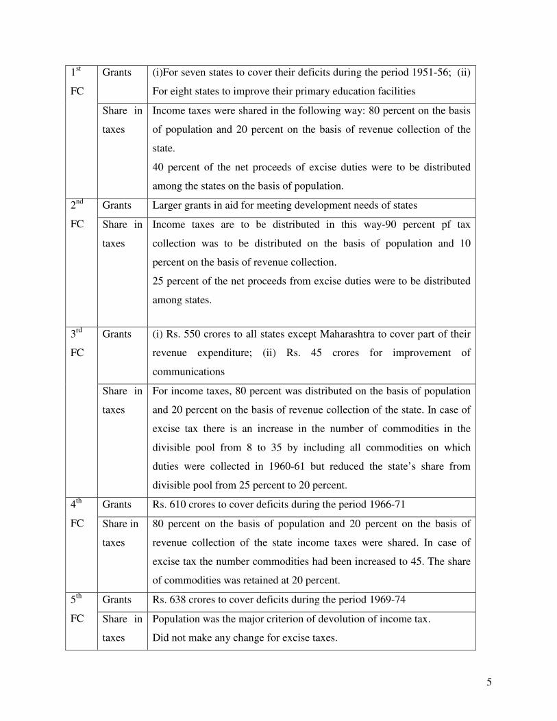
Grants (i)For seven states to cover their deficits during the period 1951-56; (ii)
For eight states to improve their primary education facilities
1st
FC
Share in
taxes
Income taxes were shared in the following way: 80 percent on the basis
of population and 20 percent on the basis of revenue collection of the
state.
40 percent of the net proceeds of excise duties were to be distributed
among the states on the basis of population.
Grants Larger grants in aid for meeting development needs of states 2nd
FC Share in
taxes
Income taxes are to be distributed in this way-90 percent pf tax
collection was to be distributed on the basis of population and 10
percent on the basis of revenue collection.
25 percent of the net proceeds from excise duties were to be distributed
among states.
Grants (i) Rs. 550 crores to all states except Maharashtra to cover part of their
revenue expenditure; (ii) Rs. 45 crores for improvement of
communications
3rd
FC
Share in
taxes
For income taxes, 80 percent was distributed on the basis of population
and 20 percent on the basis of revenue collection of the state. In case of
excise tax there is an increase in the number of commodities in the
divisible pool from 8 to 35 by including all commodities on which
duties were collected in 1960-61 but reduced the state’s share from
divisible pool from 25 percent to 20 percent.
Grants Rs. 610 crores to cover deficits during the period 1966-71 4th
FC Share in
taxes
80 percent on the basis of population and 20 percent on the basis of
revenue collection of the state income taxes were shared. In case of
excise tax the number commodities had been increased to 45. The share
of commodities was retained at 20 percent.
Grants Rs. 638 crores to cover deficits during the period 1969-74 5th
FC Share in
taxes
Population was the major criterion of devolution of income tax.
Did not make any change for excise taxes.
6
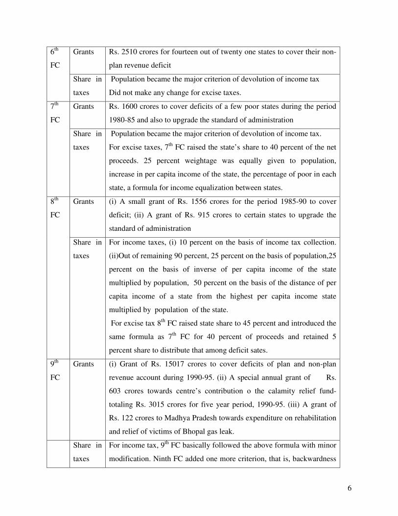
Grants Rs. 2510 crores for fourteen out of twenty one states to cover their non-
plan revenue deficit
6th
FC
Share in
taxes
Population became the major criterion of devolution of income tax
Did not make any change for excise taxes.
Grants Rs. 1600 crores to cover deficits of a few poor states during the period
1980-85 and also to upgrade the standard of administration
7th
FC
Share in
taxes
Population became the major criterion of devolution of income tax.
For excise taxes, 7th
FC raised the state’s share to 40 percent of the net
proceeds. 25 percent weightage was equally given to population,
increase in per capita income of the state, the percentage of poor in each
state, a formula for income equalization between states.
Grants (i) A small grant of Rs. 1556 crores for the period 1985-90 to cover
deficit; (ii) A grant of Rs. 915 crores to certain states to upgrade the
standard of administration
8th
FC
Share in
taxes
For income taxes, (i) 10 percent on the basis of income tax collection.
(ii)Out of remaining 90 percent, 25 percent on the basis of population,25
percent on the basis of inverse of per capita income of the state
multiplied by population, 50 percent on the basis of the distance of per
capita income of a state from the highest per capita income state
multiplied by population of the state.
For excise tax 8th
FC raised state share to 45 percent and introduced the
same formula as 7th
FC for 40 percent of proceeds and retained 5
percent share to distribute that among deficit sates.
9th
FC
Grants (i) Grant of Rs. 15017 crores to cover deficits of plan and non-plan
revenue account during 1990-95. (ii) A special annual grant of Rs.
603 crores towards centre’s contribution o the calamity relief fund-
totaling Rs. 3015 crores for five year period, 1990-95. (iii) A grant of
Rs. 122 crores to Madhya Pradesh towards expenditure on rehabilitation
and relief of victims of Bhopal gas leak.
Share in
taxes
For income tax, 9th
FC basically followed the above formula with minor
modification. Ninth FC added one more criterion, that is, backwardness
7
of sates based on population of scheduled castes and scheduled tribes,
number of agricultural labourers in different states as revealed in 1981
census. According to NFC the composite index would correctly reflect
poverty and backwardness of a state in large measure. The states having
larger share of these components were required to bear substantial
expenditure responsibilities.
For excise taxes, 9th
FC proposed to distribute the entire amount of 45
percent as a consolidated amount. The formula used was: 25 percent on
the basis of 1971 census, 12.5 percent on the basis of index of
backwardness, 33.5 percent on the basis of per capita income of the
state from highest per capita income state, 12.5 percent on the basis of
income adjusted total population, 16.5 percent among states with
deficits, after taking into account their shares from all sharable taxes.
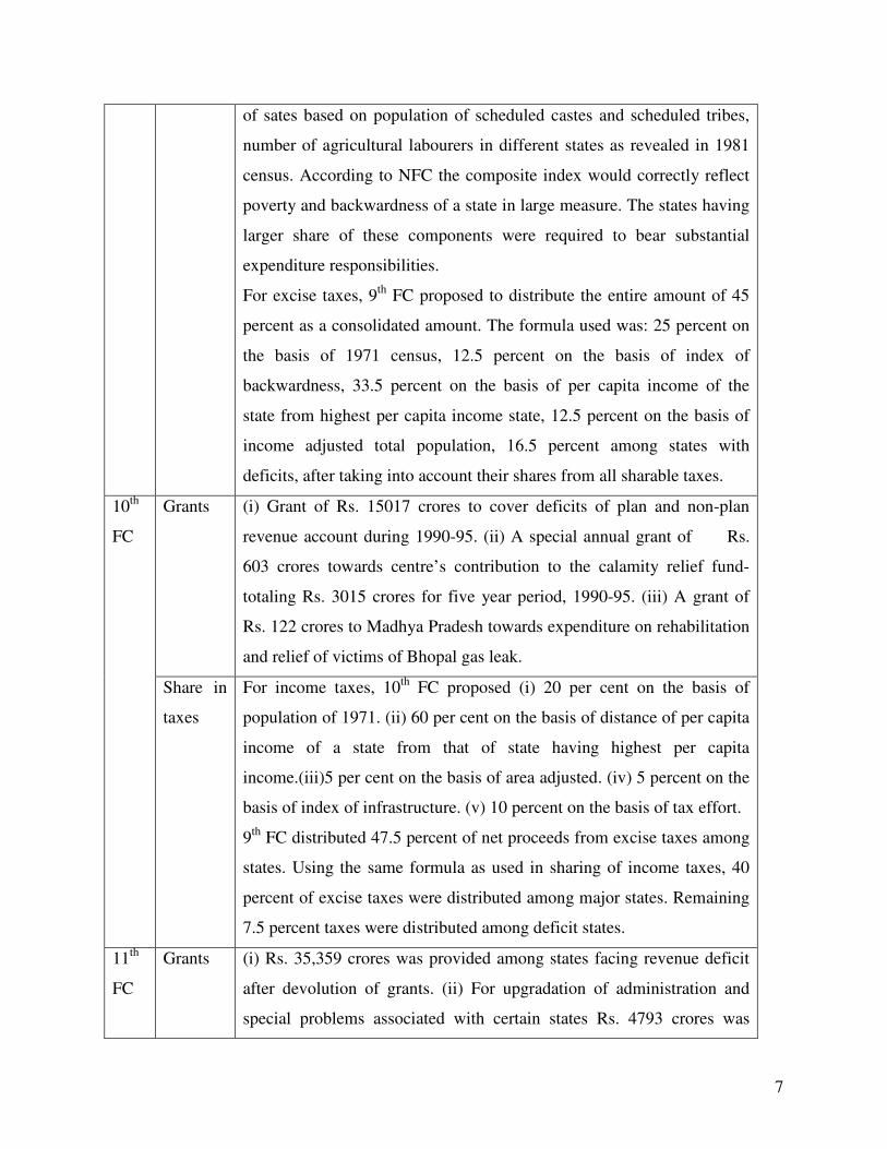
Grants (i) Grant of Rs. 15017 crores to cover deficits of plan and non-plan
revenue account during 1990-95. (ii) A special annual grant of Rs.
603 crores towards centre’s contribution to the calamity relief fund-
totaling Rs. 3015 crores for five year period, 1990-95. (iii) A grant of
Rs. 122 crores to Madhya Pradesh towards expenditure on rehabilitation
and relief of victims of Bhopal gas leak.
10th
FC
Share in
taxes
For income taxes, 10th
FC proposed (i) 20 per cent on the basis of
population of 1971. (ii) 60 per cent on the basis of distance of per capita
income of a state from that of state having highest per capita
income.(iii)5 per cent on the basis of area adjusted. (iv) 5 percent on the
basis of index of infrastructure. (v) 10 percent on the basis of tax effort.
9th
FC distributed 47.5 percent of net proceeds from excise taxes among
states. Using the same formula as used in sharing of income taxes, 40
percent of excise taxes were distributed among major states. Remaining
7.5 percent taxes were distributed among deficit states.
11th
FC
Grants (i) Rs. 35,359 crores was provided among states facing revenue deficit
after devolution of grants. (ii) For upgradation of administration and
special problems associated with certain states Rs. 4793 crores was
8
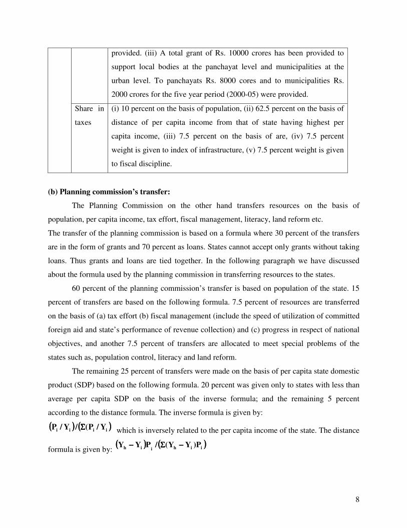
provided. (iii) A total grant of Rs. 10000 crores has been provided to
support local bodies at the panchayat level and municipalities at the
urban level. To panchayats Rs. 8000 cores and to municipalities Rs.
2000 crores for the five year period (2000-05) were provided.
Share in
taxes
(i) 10 percent on the basis of population, (ii) 62.5 percent on the basis of
distance of per capita income from that of state having highest per
capita income, (iii) 7.5 percent on the basis of are, (iv) 7.5 percent
weight is given to index of infrastructure, (v) 7.5 percent weight is given
to fiscal discipline.
(b) Planning commission’s transfer:
The Planning Commission on the other hand transfers resources on the basis of
population, per capita income, tax effort, fiscal management, literacy, land reform etc.
The transfer of the planning commission is based on a formula where 30 percent of the transfers
are in the form of grants and 70 percent as loans. States cannot accept only grants without taking
loans. Thus grants and loans are tied together. In the following paragraph we have discussed
about the formula used by the planning commission in transferring resources to the states.
60 percent of the planning commission’s transfer is based on population of the state. 15
percent of transfers are based on the following formula. 7.5 percent of resources are transferred
on the basis of (a) tax effort (b) fiscal management (include the speed of utilization of committed
foreign aid and state’s performance of revenue collection) and (c) progress in respect of national
objectives, and another 7.5 percent of transfers are allocated to meet special problems of the
states such as, population control, literacy and land reform.
The remaining 25 percent of transfers were made on the basis of per capita state domestic
product (SDP) based on the following formula. 20 percent was given only to states with less than
average per capita SDP on the basis of the inverse formula; and the remaining 5 percent
according to the distance formula. The inverse formula is given by:
(((( )))) (((( ))))iiii Y/P(/Y/P ΣΣΣΣ which is inversely related to the per capita income of the state. The distance
formula is given by: (((( )))) (((( ))))iihiih P)YY(/PYY −−−−ΣΣΣΣ−−−−
9
where iY and hY denote per capita SDP of the ith and the richest state respectively, iP , the
population of the ith state. The indicator increases as the distance of income of the ith state from
the richest state increases. Keeping these in mind we have used revenue effort, budgetary deficit
and distance of state per capita income from highest per capita income state as the three
important criteria in the devolution of transfer by the central government. It is also observed that
population is used as the important criterion of formula based transfer.
3. Theoretical model
Literature on intergovernmental transfer mechanism in India also recommended that
formula used in transferring funds should be simple and should not create any fiscal disincentive
in a state. In the previous section we have examined first the different criteria used by several
Finance and Planning commissions over the period. To fulfill the above objective we have
selected three important criteria such as, population, own revenue effort of the state and gap
filling to define the formula in transferring resources in India.
Instead of transfers by three different bodies separately we have analyzed the central
government’s transfers as a whole. Evaluating formula used by different Planning and Finance
commissions it is observed that population, revenue effort, deficit filling and the distance criteria
are the important criteria used by transferring agencies in India. In our model we assume a
simple formula for transferring resources to a state.
We assume here that per capita transfer to a state depends on revenue effort index, actual
deficit of the state and the distance criterion. Revenue effort index is measured by the actual
revenue2 to revenue capacity of the state, actual deficit is calculated as the difference between
actual expenditure and actual own revenue and the distance of per capita income from highest
per capita income is calculated using the formula stated below (1a). Thus transfer to a particular
state at any time period t is assumed to follow the following formula
itititititit
it DI)TG()TT(P
Trδ+−β+−α= , t=1,2,3,…….. (1)
where ( )ithtit yyDI −= , )1t(iitit BEG −+=
2 Actual own revenue is defined as the sum of own tax and non-tax revenue on revenue account
and non-debt capital receipt on capital account.
10
Here i indicates ith state, itTr is the transfer to the ith state at time t, itP is the population
of the ith state at time t, Ti and itT are actual own revenue collection and the estimated revenue
capacity respectively of the ith state at time t, Git is the total expenditure by the ith state at period
t , )TG( itit − corresponds to actual budget deficit of the state i at time t, itDI is the distance of
per capita net state domestic product (NSDP) from highest per capita NSDP in India at time
period t, ity is the per capita net state domestic product of ith state at time period t, hty is the
highest per capita NSDP at time period t, )1t(iB − is the repayment of borrowing of period (t-1) in
period t, itE is the government expenditure on goods and services in period t.
It is assumed that 0,, ⟩δβα . This implies that as states give more effort to raise its own
revenue over and above their revenue capacity then transfer of funds by the central government
will increase. We also assume that as deficit of a state increases a part of the deficit will be
financed by the central government in India. For the empirical part we have used the estimated
revenue capacity as estimated by the Finance Commission. As the distance of per capita NSDP
of the state from that of state having highest per capita NSDP increases the transfer received by
the state also increases.
The budget constraint faced by the state government in a federal country like India is as follows:
itititit TrBTG ++=
ititit)1t(iit BTrTBE ++=+⇒ − (2)
itititit TrBTE ++=⇒•
itititit TrBTG)1( ++=θ−⇒•
Here we assume that θ=− t1t G/B (constant).
Substituting (4.3.1) in (4.3.2) we get,
[ ] ititititititititit PDI)TG()TT(BT)1(G δ+−β+−α++=θ−•
where ititititit
it
it DI)TG()TT(P
Trδ+−β+−α=
)1t(iitititit BTrTG)1(B −
•
−−−θ−=∴
11
)1t(iitititititititititit BDIP)TG(P)TT(PTG)1( −−δ−−β−−α−−θ−=
)1t(iit'
it'
it''
it' BDITT)1(G)1)(1( −−δ−α+β−α+−β−θ−=
)1t(iit''
it' BAT)1(G)1)(1( −−+β−α+−β−θ−= (3)
where P' α=α , P' β=β and P' δ=δ ,
it'
it'
DITA δ−α=
Here we assume that the government borrows a constant proportion of its income in each
period thus tt
t bY
B= . We also assume that tY grows at a constant annual rate of γ . Thus we
assume γ=•
)YY( tt
Now tt bYB = tttttt TrTG)1(YbYbB −−θ−=+=⇒•••
trttt
ttt
t
t g)1(Y
Ybb
Y
Bτ−τ−θ−=+=
••
•
trttt g)1(bb τ−τ−θ−=γ+⇒•
γ−τ−τ−θ−=⇒•
bg)1(btrttt
where t,Yt
Bb,
Y
T,
Y
T,
Y
Gg t
t
rttr
t
tt
t
tt ∀==τ=τ=
γ−δ−τα+τβ−α+−β−=⇒•
bdˆ)1(g)1(b t''
tt'
t (3)’
To determine the optimal own revenue and expenditure in a federal country like India where
certain proportion of revenue comes from central transfer we make the following assumptions:
(i) Same formula is used in transferring resources to all the states.
(ii) The decisions concerning both the state budget revenue formation and the procedures
of financing the corresponding expenditures are made by the state governments.
(iii) Government expenditure and revenue collection in real terms are certain proportion
of its real output. It is assumed that gYG = and YT τ= , where G: real government
expenditure, T: real revenue collection (tax, non-tax and non-debt capital receipts), Y:
real output, g is the government real expenditure as a proportion to the real output, τ
is the real revenue collection as proportion to the real output. Here T is not a function
as used in case of direct tax.
12
(iv) Public transfers are not included into regional budget expenditures.
(v) Borrowing taken in period (t-1) is repaid in period t.
(vi) Objective of the state governments is to maximize utility of the economic agents
which depends on its own expenditure and revenue policy. Increase in real
expenditure increases utility directly and increase in real revenue collection affects
utility through its impact on reduction of real output available in the hands of the
economic agents. Thus utility is function of public goods and private goods
consumption. G represents the public goods consumption while private goods
consumption is proxied by the real output less the output taken away by the
government as tax (Y-T). Utility function is defined as follows:
( ) dte)TY(,GUU t
0t
tttρ−
∞
=∫ −=
( ) dte)1(,gUY t
0t
tttρ−
∞
=∫ τ−=
( ) dteY)1ln()w1(glnw0t
t][0tt∫
∞
=
γ−ρ−τ−−+= (4)
Thus as g increases that increases regional utility and as τ increases that takes away certain
proportion of real output from the hands of the economic agents. Thus )1( τ− is the proportion
of real output available in the hands of the economic agents. Higher the value of τ lower is the
value of )1( τ− and thus lower is the utility derived by economic agents. Here ( ))w1(w −
measures the provision of public to private goods and services, ρ is the rate of time preference, γ
is the rate of growth of real output.
We maximize (4) with respect to T,G subject to the government intertemporal budget
constraint (3)’. The Hamiltonian equation for this problem is as follows
[ ]γ−δ−ταβ−α+
−+=τ bdˆ
)1(
)w1(w ''
''
* (5)
[ ]γ−δ−ταθ−β−
−θ−β−
β−α+= bdˆ
)1)(1(
w
)1)(1(
)1(wg ''
''
''* (6)
13
Thus, state authorities’ optimum choice depends upon the rules applied to regional
transfer allocation, that is δβα ,, .
Thus optimum revenue to output ratio depends positively on revenue capacity ratio and
negatively on higher transfer received on the basis of distance criterion, rate of borrowing (b) in
each period, rate of growth of real output and constant rate of repayment of borrowing as a
proportion to total government expenditure (θ) . This means that the state with higher the
revenue capacity can collect more revenue and poorer the state, the more is the transfer received
by the state and lower is optimum revenue collection. Again more it can borrow lower is the
state’s revenue collection.
Higher the revenue capacity ratio lower is the transfer received and thus lower is the
optimum expenditure to output ratio. Poorer the state is higher will be transfer received on the
basis of distance criterion and this will affect the optimum expenditure to output ratio positively.
More the state can borrow the more it will be able to spend. Thus borrowing rate affects the
optimum expenditure to output ratio positively.
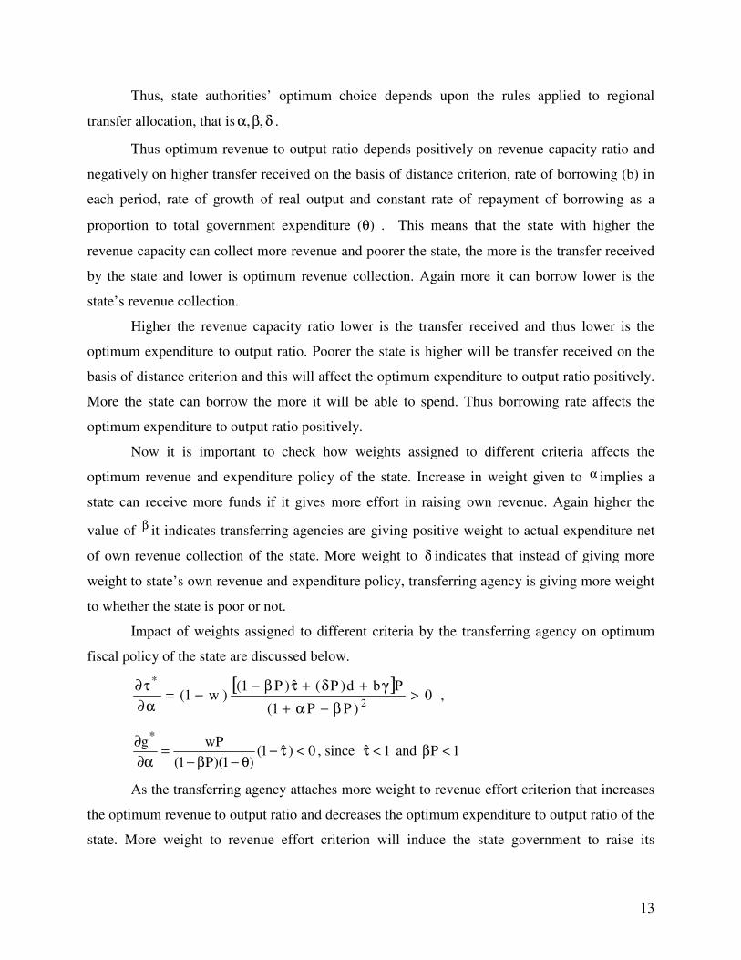
Now it is important to check how weights assigned to different criteria affects the
optimum revenue and expenditure policy of the state. Increase in weight given to α implies a
state can receive more funds if it gives more effort in raising own revenue. Again higher the
value of β it indicates transferring agencies are giving positive weight to actual expenditure net
of own revenue collection of the state. More weight to δ indicates that instead of giving more
weight to state’s own revenue and expenditure policy, transferring agency is giving more weight
to whether the state is poor or not.
Impact of weights assigned to different criteria by the transferring agency on optimum
fiscal policy of the state are discussed below.
[ ]0
)PP1(
Pbd)P(ˆ)P1()w1(
2
*
>β−α+
γ+δ+τβ−−=
α∂
τ∂ ,
0)ˆ1()1)(P1(
wPg*
<τ−θ−β−
=α∂
∂, since 1ˆ <τ and 1P <β
As the transferring agency attaches more weight to revenue effort criterion that increases
the optimum revenue to output ratio and decreases the optimum expenditure to output ratio of the
state. More weight to revenue effort criterion will induce the state government to raise its
14
revenue collection to get the same level of transfer. Given the revenue effort of the government
more weight to α will increase the revenue side of the government budget and thus given the
budget constraint optimum expenditure to output ratio will increase. This means that as α
increases optimum policy of the government will be to raise revenue more. Now as state’s
revenue collection increases this will have negative influence on regional utility. Now to increase
utility the state government’s optimum policy will be to increase expenditure to output ratio.
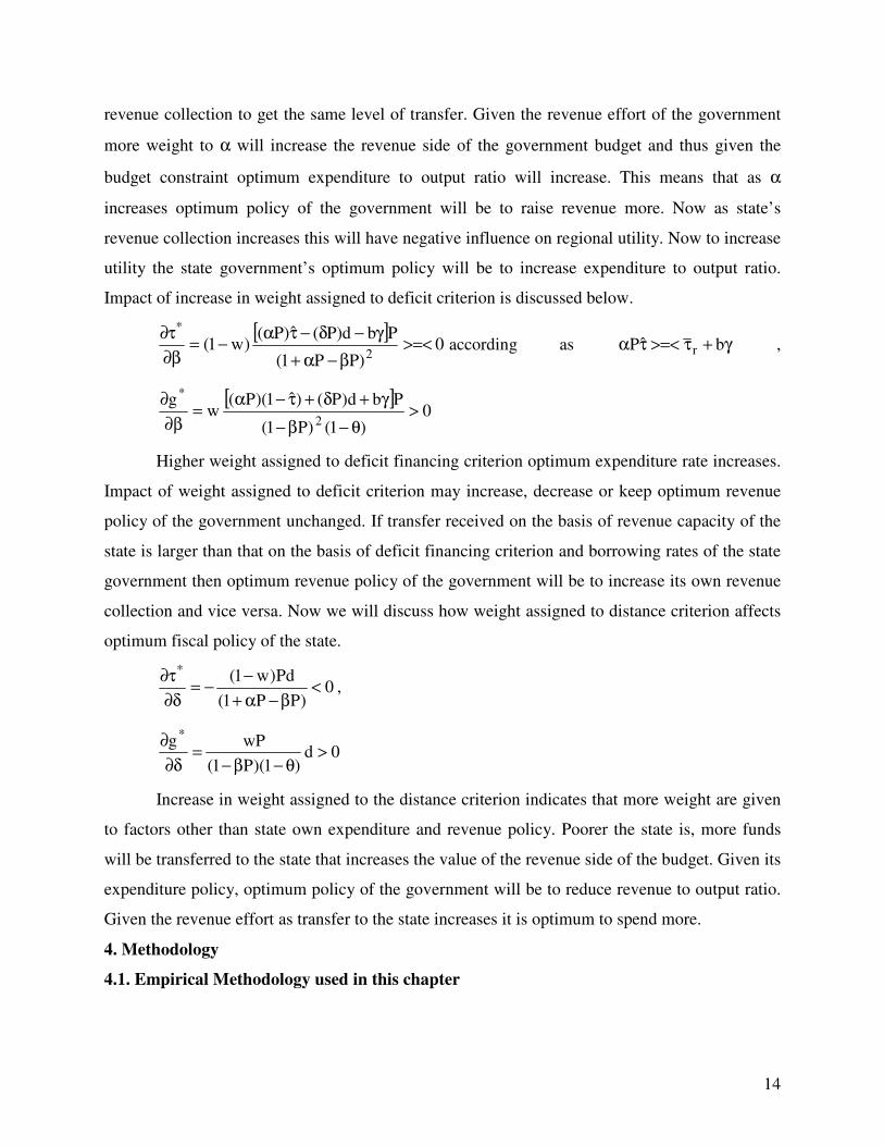
Impact of increase in weight assigned to deficit criterion is discussed below.
[ ]0
)PP1(
Pbd)P(ˆ)P()w1(
2
*
>=<β−α+
γ−δ−τα−=
β∂
τ∂according as γ+τ>=<τα bˆP r ,
[ ]0
)1()P1(
Pbd)P()ˆ1)(P(w
g
2
*
>θ−β−
γ+δ+τ−α=
β∂
∂
Higher weight assigned to deficit financing criterion optimum expenditure rate increases.
Impact of weight assigned to deficit criterion may increase, decrease or keep optimum revenue
policy of the government unchanged. If transfer received on the basis of revenue capacity of the
state is larger than that on the basis of deficit financing criterion and borrowing rates of the state
government then optimum revenue policy of the government will be to increase its own revenue
collection and vice versa. Now we will discuss how weight assigned to distance criterion affects
optimum fiscal policy of the state.
0)PP1(
Pd)w1(*
<β−α+
−−=
δ∂
τ∂,
0d)1)(P1(
wPg*
>θ−β−
=δ∂
∂
Increase in weight assigned to the distance criterion indicates that more weight are given
to factors other than state own expenditure and revenue policy. Poorer the state is, more funds
will be transferred to the state that increases the value of the revenue side of the budget. Given its
expenditure policy, optimum policy of the government will be to reduce revenue to output ratio.
Given the revenue effort as transfer to the state increases it is optimum to spend more.
4. Methodology
4.1. Empirical Methodology used in this chapter
15
Ordinary least square method is used on pooled data taken from five selected states in
India over the period 1981 to 2001. We have estimated the parameters of the transfer formula
using the following regression model.
( )[ ] ( )[ ] it54210itititit
u5Dc4Dc2Dc1DccDITGTTP
Tr++++++δ+−β+−α=
where D1=Andhra Pradesh, D2=Karnataka, D3= Orissa, D4=Tamil Nadu, D5= West
Bengal. Di=1 for ith state, =0 otherwise, iu is the random disturbance term. To estimate the
coefficients of the above model and eliminate the problem of dummy variable trap we have
excluded D3 that is, Orissa and applied ordinary least square method to the above equation.
( )tPTr is the per capita transfer at time period t, t)TT( − is defied as the revenue effort by the
state over and above their revenue capacity at time period t, (G-T)t is the difference between the
total public expenditure and own revenue collection of the state. DIt is the distance of per capita
income of the state from highest per capita income of fifteen major states in India.
To find out whether the error in prediction is significantly different from zero or not the
pair difference t-test is used. The test statistic that we have used is n/s
0et
1n1n,025.0
−−
−=
where n is the number of pairs or number of differences and sn-1 is the sample standard deviation
of e for n-1 observations.
Using the estimated coefficients from the above model optimum revenue to output ratio
and the optimum expenditure to output ratio are calculated using equations (5) and (6). Actual
rates are compared with the optimum rates in order to find out the possible direction of fiscal
policy at the state level.
Mean of the absolute difference between actual and predicted values relative to actual
values is used as a measure of mean relative error in prediction. Thus mean relative error in
prediction is calculated using the following formula:
−∑
=i
n
1ii
*i xxx
n
1 ,
where ix is the actual value of the variable, *ix is the optimum value of ix , n is number of
observations.
4.2. Methodology used by Finance Commission in calculating tax capacity
The way the Finance Commission has estimated the taxable capacity of a state is
explained below. Taxable capacities of the states for each of the major taxes are calculated first
16
then summing them up the ninth finance commission has estimated the aggregate taxable
capacity of the state. Taxes are categorized into six major heads namely: (i) Sales tax (including
central sales tax and purchase tax on sugarcane), (ii) state excise duties, (iii) stamp duties and
registration fees, (iv) motor vehicles tax and passenger and goods tax, (v) entertainment tax, (vi)
tax on agriculture and incomes and a residual category, other taxes.
It is difficult to calculate the revenues from agricultural income taxes and other taxes
using statistical method. The taxable capacities of this category of taxes are calculated on the
basis of projected actual taxes. Taxable capacities of other five categories of taxes have been
calculated using pooled time series and cross section data. It is assumed that there is no state
specific variation. Thus it is assumed that the intercept and slope parameters are same across
states. Time dummies are introduced in the model to capture the inter-temporal shifts. States are
divided into three income groups, high income, middle income and low-income group.
For different categories of taxes different variables are considered and taxable capacities
are estimated for each of the income groups. The variables that are used to estimate the tax
capacities are as follows: State domestic product at factor cost, roads/railway length per 1000
square kilometer, per capita energy sale to ultimate consumer, total registered motor vehicles,
proportion of heavy vehicles to total vehicles, consumption of country spirit (PL), seating
capacities in cinema hall, proportion of urban population to total population while time dummies
are introduced to capture inter-temporal shifts. The ninth Finance Commission has estimated
taxable capacities for the period 1989-90 to 1994-95.
4.3. Methodology used in this paper in calculating revenue capacity of state
Using the estimated taxable capacities we have estimated the taxable capacities to other
years within the period 1981 to 2001. First, we have found the actual ratio of non-tax and tax
revenue at constant prices for various years. Then three years moving average method is used.
Average of these averages is used to calculate the total revenue (tax + non-tax) capacities of the
state.
5. Data Source and Variables
5.1. Data Source:
This section summarizes the data used in this study. In this chapter we consider the
period 1981 to 2001, using data on five states of India. State finance data such as data on grants -
in - aid, share in central taxes, loans and advances by the central government, borrowing,
17
expenditure on revenue and capital account, own revenue collection of the states are collected
from various issues of “State Finances: A study of budgets” published by Reserve Bank of India,
India. Revenue capacity of the states is obtained by using the estimated tax capacity data by the
finance commission for the period 1989-90 to 1994-95.
5.2. Variables:
The variables3 that have been used in the empirical estimation of the model are defined
below: Y: Gross State Domestic Product (GSDP) at constant 1993-94 prices4 Tr: Transfer of the
central Government= Share in central taxes, grants and loans; Bt: Borrowing from all sources
other than central government, Bt-1: Repayment of loans taken in period (t-1) from sources other
than loans from the central government; G: State own expenditure net of transfers =Revenue
Expenditure + Capital expenditure –Grants and loans other than central ministries grants5; T:
Actual Revenue=Own Tax + Own Non-Tax Revenue + non-debt capital receipt; T =Own
Revenue capacity6, DI: distance of per capita income of the state from highest per capita income
multiplied by population relative to the over all distance of income over the fifteen major states
in India.
6. Empirical Analysis
6.1. Estimation of per capita transfer
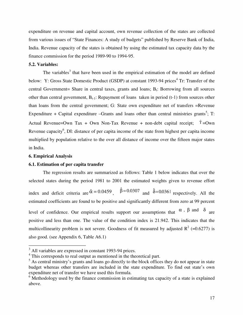
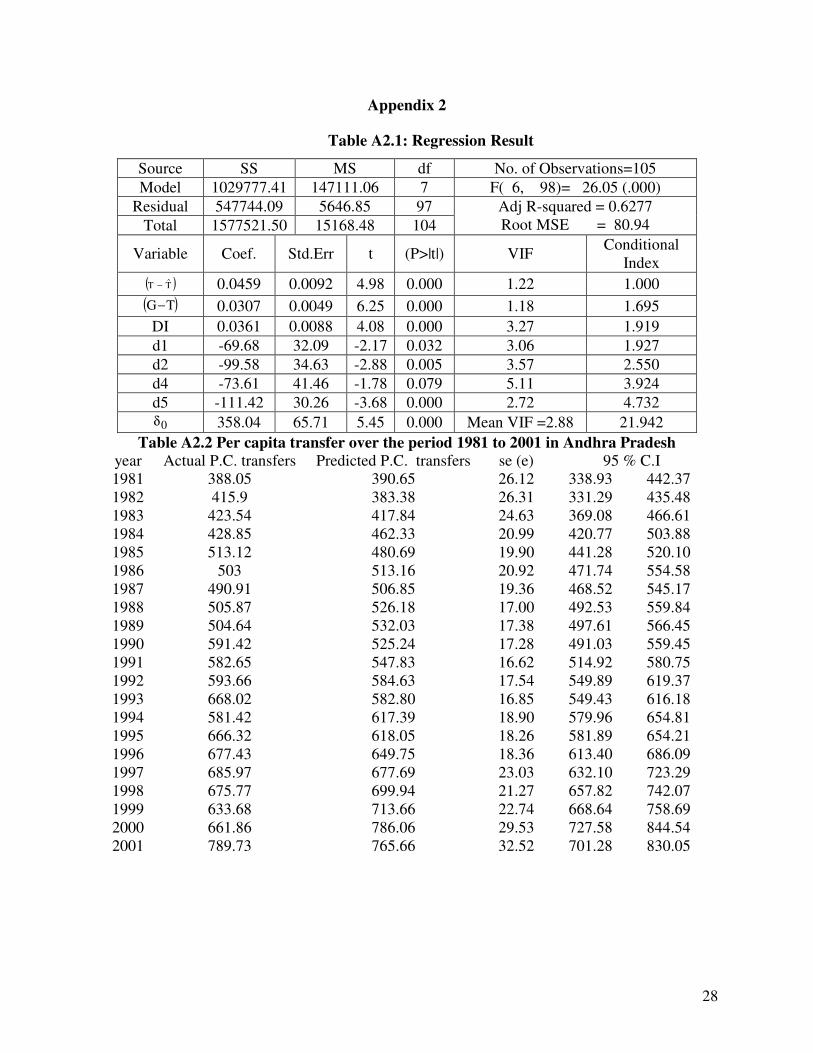
The regression results are summarized as follows: Table 1 below indicates that over the
selected states during the period 1981 to 2001 the estimated weights given to revenue effort
index and deficit criteria are 0459.0ˆ =α , 0307.0ˆ =β
and 0361.0ˆ =δ respectively. All the
estimated coefficients are found to be positive and significantly different from zero at 99 percent
level of confidence. Our empirical results support our assumptions that δβα and,
are
positive and less than one. The value of the condition index is 21.942. This indicates that the
multicollinearity problem is not severe. Goodness of fit measured by adjusted R2 (=0.6277) is
also good. (see Appendix 6, Table A6.1)
3 All variables are expressed in constant 1993-94 prices.
4 This corresponds to real output as mentioned in the theoretical part.
5 As central ministry’s grants and loans go directly to the block offices they do not appear in state
budget whereas other transfers are included in the state expenditure. To find out state’s own
expenditure net of transfer we have used this formula. 6 Methodology used by the finance commission in estimating tax capacity of a state is explained
above.
18
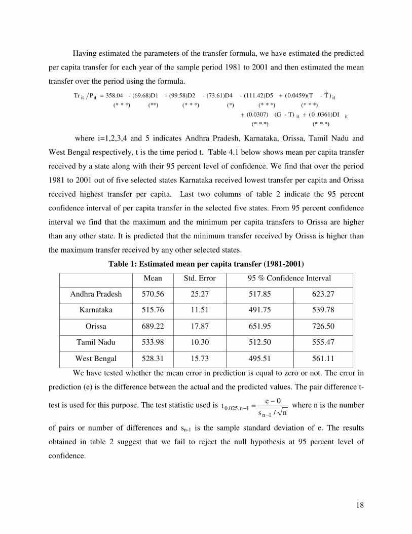
Having estimated the parameters of the transfer formula, we have estimated the predicted
per capita transfer for each year of the sample period 1981 to 2001 and then estimated the mean
transfer over the period using the formula.
*)*(* *)*(*
.0361)DI 0(T)-(G (0.0307)
*)*(* *)*(* (*) *)*(*(**) *)*(*
)T-0.0459)(T((111.42)D5-(73.61)D4-(99.58)D2-(69.68)D1-358.04 PTr
itit
ititit
++
+=
where i=1,2,3,4 and 5 indicates Andhra Pradesh, Karnataka, Orissa, Tamil Nadu and
West Bengal respectively, t is the time period t. Table 4.1 below shows mean per capita transfer
received by a state along with their 95 percent level of confidence. We find that over the period
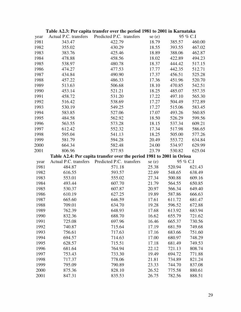
1981 to 2001 out of five selected states Karnataka received lowest transfer per capita and Orissa
received highest transfer per capita. Last two columns of table 2 indicate the 95 percent
confidence interval of per capita transfer in the selected five states. From 95 percent confidence
interval we find that the maximum and the minimum per capita transfers to Orissa are higher
than any other state. It is predicted that the minimum transfer received by Orissa is higher than
the maximum transfer received by any other selected states.
Table 1: Estimated mean per capita transfer (1981-2001)
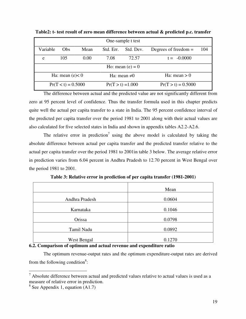
We have tested whether the mean error in prediction is equal to zero or not. The error in
prediction (e) is the difference between the actual and the predicted values. The pair difference t-
test is used for this purpose. The test statistic used is n/s
0et
1n
1n,025.0
−−
−= where n is the number
of pairs or number of differences and sn-1 is the sample standard deviation of e. The results
obtained in table 2 suggest that we fail to reject the null hypothesis at 95 percent level of
confidence.
Mean Std. Error 95 % Confidence Interval
Andhra Pradesh 570.56 25.27 517.85 623.27
Karnataka 515.76 11.51 491.75 539.78
Orissa 689.22 17.87 651.95 726.50
Tamil Nadu 533.98 10.30 512.50 555.47
West Bengal 528.31 15.73 495.51 561.11
19
Table2: t- test result of zero mean difference between actual & predicted p.c. transfer
One-sample t test
Variable Obs Mean Std. Err. Std. Dev. Degrees of freedom = 104
e 105 0.00 7.08 72.57 t = -0.0000
Ho: mean (e) = 0
Ha: mean (e)< 0 Ha: mean ≠0 Ha: mean > 0
Pr(T < t) = 0.5000 Pr(T > t) =1.000 Pr(T > t) = 0.5000
The difference between actual and the predicted value are not significantly different from
zero at 95 percent level of confidence. Thus the transfer formula used in this chapter predicts
quite well the actual per capita transfer to a state in India. The 95 percent confidence interval of
the predicted per capita transfer over the period 1981 to 2001 along with their actual values are
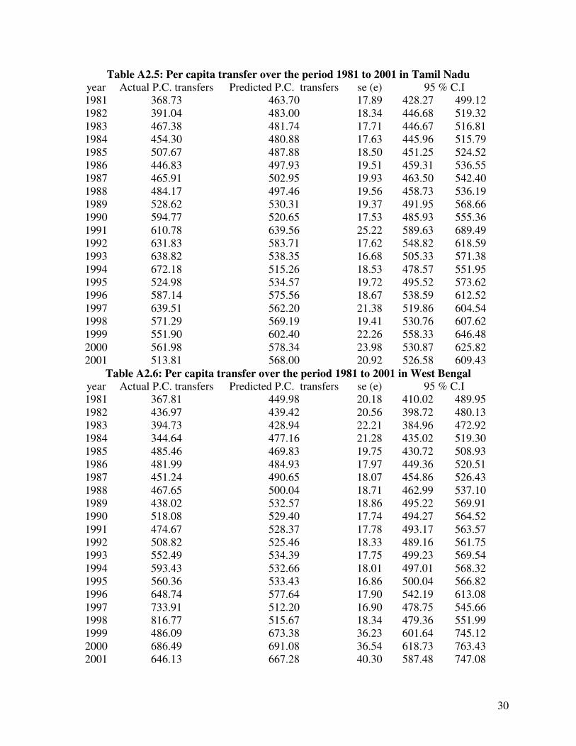
also calculated for five selected states in India and shown in appendix tables A2.2-A2.6.
The relative error in prediction7 using the above model is calculated by taking the
absolute difference between actual per capita transfer and the predicted transfer relative to the
actual per capita transfer over the period 1981 to 2001in table 3 below. The average relative error
in prediction varies from 6.04 percent in Andhra Pradesh to 12.70 percent in West Bengal over
the period 1981 to 2001.
Table 3: Relative error in prediction of per capita transfer (1981-2001)
Mean
Andhra Pradesh 0.0604
Karnataka 0.1046
Orissa 0.0798
Tamil Nadu 0.0892
West Bengal 0.1270
6.2. Comparison of optimum and actual revenue and expenditure ratio
The optimum revenue-output rates and the optimum expenditure-output rates are derived
from the following condition8:
7 Absolute difference between actual and predicted values relative to actual values is used as a
measure of relative error in prediction. 8 See Appendix 1, equation (A1.7)
20
)1()1)(1(
)1(
w1
wg
'
''
τ−θ−β−
β−α+
−
= .
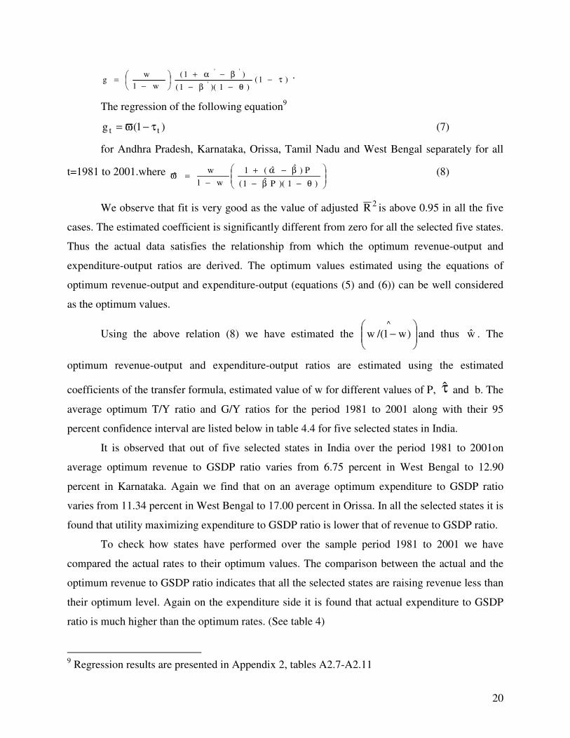
The regression of the following equation9
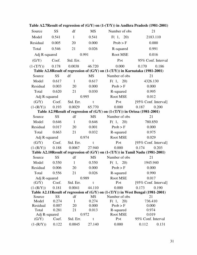
)1(g tt τ−ϖ= (7)
for Andhra Pradesh, Karnataka, Orissa, Tamil Nadu and West Bengal separately for all
t=1981 to 2001.where
θ−β−
β−α+
−=ϖ
)1)(Pˆ1(
P)ˆˆ(1
w1
wˆ (8)
We observe that fit is very good as the value of adjusted 2R is above 0.95 in all the five
cases. The estimated coefficient is significantly different from zero for all the selected five states.
Thus the actual data satisfies the relationship from which the optimum revenue-output and
expenditure-output ratios are derived. The optimum values estimated using the equations of
optimum revenue-output and expenditure-output (equations (5) and (6)) can be well considered
as the optimum values.
Using the above relation (8) we have estimated the
−
^
)w1/(w and thus w . The
optimum revenue-output and expenditure-output ratios are estimated using the estimated
coefficients of the transfer formula, estimated value of w for different values of P, τ and b. The
average optimum T/Y ratio and G/Y ratios for the period 1981 to 2001 along with their 95
percent confidence interval are listed below in table 4.4 for five selected states in India.
It is observed that out of five selected states in India over the period 1981 to 2001on
average optimum revenue to GSDP ratio varies from 6.75 percent in West Bengal to 12.90
percent in Karnataka. Again we find that on an average optimum expenditure to GSDP ratio
varies from 11.34 percent in West Bengal to 17.00 percent in Orissa. In all the selected states it is
found that utility maximizing expenditure to GSDP ratio is lower that of revenue to GSDP ratio.
To check how states have performed over the sample period 1981 to 2001 we have
compared the actual rates to their optimum values. The comparison between the actual and the
optimum revenue to GSDP ratio indicates that all the selected states are raising revenue less than
their optimum level. Again on the expenditure side it is found that actual expenditure to GSDP
ratio is much higher than the optimum rates. (See table 4)
9 Regression results are presented in Appendix 2, tables A2.7-A2.11
21
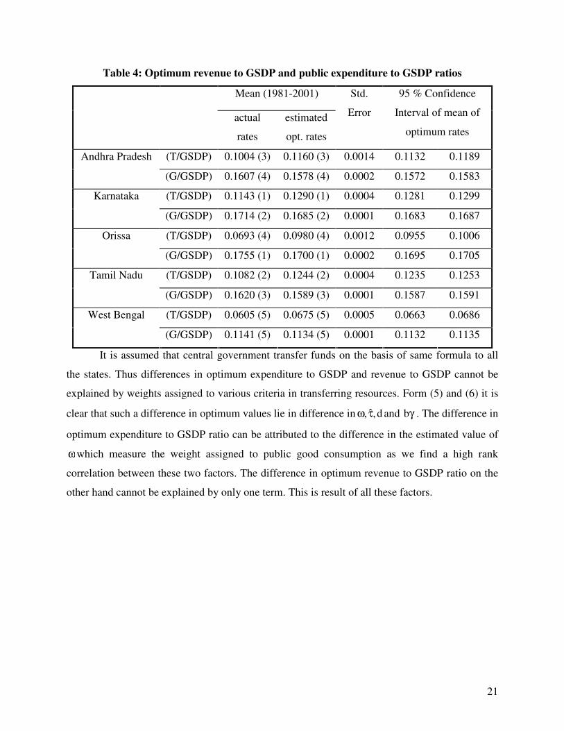
Table 4: Optimum revenue to GSDP and public expenditure to GSDP ratios
It is assumed that central government transfer funds on the basis of same formula to all
the states. Thus differences in optimum expenditure to GSDP and revenue to GSDP cannot be
explained by weights assigned to various criteria in transferring resources. Form (5) and (6) it is
clear that such a difference in optimum values lie in difference in γτω bandd,ˆ, . The difference in
optimum expenditure to GSDP ratio can be attributed to the difference in the estimated value of
ωwhich measure the weight assigned to public good consumption as we find a high rank
correlation between these two factors. The difference in optimum revenue to GSDP ratio on the
other hand cannot be explained by only one term. This is result of all these factors.
Mean (1981-2001)
actual
rates
estimated
opt. rates
Std.
Error
95 % Confidence
Interval of mean of
optimum rates
(T/GSDP) 0.1004 (3) 0.1160 (3) 0.0014 0.1132 0.1189 Andhra Pradesh
(G/GSDP) 0.1607 (4) 0.1578 (4) 0.0002 0.1572 0.1583
(T/GSDP) 0.1143 (1) 0.1290 (1) 0.0004 0.1281 0.1299 Karnataka
(G/GSDP) 0.1714 (2) 0.1685 (2) 0.0001 0.1683 0.1687
(T/GSDP) 0.0693 (4) 0.0980 (4) 0.0012 0.0955 0.1006 Orissa
(G/GSDP) 0.1755 (1) 0.1700 (1) 0.0002 0.1695 0.1705
(T/GSDP) 0.1082 (2) 0.1244 (2) 0.0004 0.1235 0.1253 Tamil Nadu
(G/GSDP) 0.1620 (3) 0.1589 (3) 0.0001 0.1587 0.1591
(T/GSDP) 0.0605 (5) 0.0675 (5) 0.0005 0.0663 0.0686 West Bengal
(G/GSDP) 0.1141 (5) 0.1134 (5) 0.0001 0.1132 0.1135
22
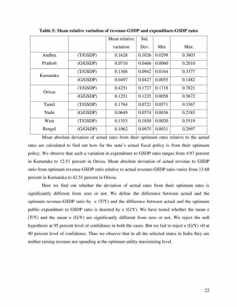
Table 5: Mean relative variation of revenue-GSDP and expenditure-GSDP rates
Mean relative
variation
Std.
Dev. Min Max
(T/GSDP) 0.1628 0.1026 0.0299 0.3803 Andhra
Pradesh (G/GSDP) 0.0710 0.0466 0.0060 0.2010
(T/GSDP) 0.1368 0.0942 0.0164 0.3377 Karnataka
(G/GSDP) 0.0497 0.0427 0.0055 0.1482
(T/GSDP) 0.4251 0.1727 0.1718 0.7821 Orissa
(G/GSDP) 0.1251 0.1235 0.0058 0.5672
(T/GSDP) 0.1764 0.0721 0.0571 0.3367 Tamil
Nadu (G/GSDP) 0.0649 0.0574 0.0036 0.2183
(T/GSDP) 0.1553 0.1850 0.0020 0.5519 West
Bengal (G/GSDP) 0.1062 0.0975 0.0031 0.2997
Mean absolute deviation of actual rates from their optimum rates relative to the actual
rates are calculated to find out how far the state’s actual fiscal policy is from their optimum
policy. We observe that such a variation in expenditure to GSDP ratio ranges from 4.97 percent
in Karnataka to 12.51 percent in Orissa. Mean absolute deviation of actual revenue to GSDP
ratio from optimum revenue-GSDP ratio relative to actual revenue-GSDP ratio varies from 13.68
percent in Karnataka to 42.51 percent in Orissa.
Here we find out whether the deviation of actual rates from their optimum rates is
significantly different from zero or not. We define the difference between actual and the
optimum revenue-GSDP ratio by e (T/Y) and the difference between actual and the optimum
public expenditure to GSDP ratio is denoted by e (G/Y). We have tested whether the mean e
(T/Y) and the mean e (G/Y) are significantly different from zero or not. We reject the null
hypothesis at 95 percent level of confidence in both the cases. But we fail to reject e (G/Y) =0 at
90 percent level of confidence. Thus we observe that in all the selected states in India they are
neither raising revenue nor spending at the optimum utility maximizing level.
23
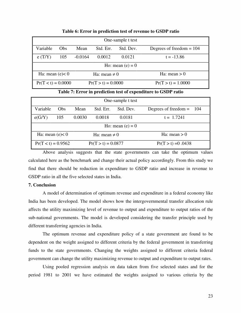
Table 6: Error in prediction test of revenue to GSDP ratio
One-sample t test
Variable Obs Mean Std. Err. Std. Dev. Degrees of freedom = 104
e (T/Y) 105 -0.0164 0.0012 0.0121 t = -13.86
Ho: mean (e) = 0
Ha: mean (e)< 0 Ha: mean ≠ 0 Ha: mean > 0
Pr(T < t) = 0.0000 Pr(T > t) = 0.0000 Pr(T > t) = 1.0000
Table 7: Error in prediction test of expenditure to GSDP ratio
One-sample t test
Variable Obs Mean Std. Err. Std. Dev. Degrees of freedom = 104
e(G/Y) 105 0.0030 0.0018 0.0181 t = 1.7241
Ho: mean (e) = 0
Ha: mean (e)< 0 Ha: mean ≠ 0 Ha: mean > 0
Pr(T < t) = 0.9562 Pr(T > t) = 0.0877 Pr(T > t) =0 .0438
Above analysis suggests that the state governments can take the optimum values
calculated here as the benchmark and change their actual policy accordingly. From this study we
find that there should be reduction in expenditure to GSDP ratio and increase in revenue to
GSDP ratio in all the five selected states in India.
7. Conclusion
A model of determination of optimum revenue and expenditure in a federal economy like
India has been developed. The model shows how the intergovernmental transfer allocation rule
affects the utility maximizing level of revenue to output and expenditure to output ratios of the
sub-national governments. The model is developed considering the transfer principle used by
different transferring agencies in India.
The optimum revenue and expenditure policy of a state government are found to be
dependent on the weight assigned to different criteria by the federal government in transferring
funds to the state governments. Changing the weights assigned to different criteria federal
government can change the utility maximizing revenue to output and expenditure to output rates.
Using pooled regression analysis on data taken from five selected states and for the
period 1981 to 2001 we have estimated the weights assigned to various criteria by the
24
transferring agencies. These coefficients are thus statistically estimated not arbitrarily chosen.
All the coefficients are found to be significantly different from zero at 5 percent level of
significance. All the dummy variables are also found to be significant at 5 percent level of
significance. As we have assumed in the theoretical part all the coefficients are found to be
positive in sign.
We find that on an average Orissa received the largest per capita transfer. On the other
hand Karnataka received the lowest funds per capita from the centre over the period 1981 to
2001 out of the five selected states. Average per capita transfer during this period was also very
high in Andhra Pradesh. Population in West Bengal is highest out of five selected states but
estimated mean per capita transfer is higher than that in Karnataka. This implies that West
Bengal received higher total transfer than Karnataka during this period. Formula considered in
this chapter predicts quite well the actual per capita transfer to a state in India as we fail to reject
the null hypothesis of zero mean error in prediction at 95 percent level of confidence.
Optimum revenue and expenditure rates are obtained substituting the estimated
coefficients of the transfer formula. The actual revenue to GSDP ratio is found to be lower than
the optimum revenue to GSDP ratio in all the selected states. On the other hand, actual
expenditure to GSDP ratios in five selected states is higher than their optimum values. Given the
transfer formula and the estimated parameters of the model, the optimum revenue and
expenditure to GSDP ratios calculated here can be considered as the benchmark by the state
governments. The deviation of actual values from the optimum values also give us some idea
regarding to which direction the state governments should change its existing revenue and
expenditure policies.
Bibliography
Bhal, R.W. (1971). A regression Approach to Tax Effort and Tax Ratio Analysis, IMF Staff
Papers, International Monetary Fund, 18 (3):570-612
Bajpai, N. and Sachs., J.D. (1999). The State of State Government Finances in India.
Development Discussion Paper No. 719, http://www.ksg.harvard.edu/CID/india/pdfs/719.pdf
Coondoo, D., Majumder, A., Mukherjee, R., Neogi, C., (2001). Relative Tax Performances
Analysis for Selected States in India, Economic and political weekly, 36(40): 3869-3871
Coondoo, D., Majumder, A., Neogi., C. (2000), “Taxable Capacity Function: A Note on
Specification, Estimation and Application”, in in D. K. Srivastava (ed.), Fiscal Federalism in
25
India: Contemporary Issues, Har-Anand Publications, New
Delhi, 166-179.
Dahlby, B.(2004), “The Marginal Cost of Funds from Public Sector Borrowing”, Department of
Economics, University of Alberta, revised September 2004,
http://www.uofaweb.ualberta.ca/ipe/pdfs/DahlbyTheMCFfromPublicSectorBorrowingDec04.pdf
GR (2001). Impact of Grants on Tax Effort of Local Government, Economic and Political
Weekly, 36(41):4231
Government of Gujarat (2003), “Memorandum to the Twelfth Finance Commission”, Finance
Commission, India, http://fincomindia.nic.in/pubsugg/memo_guj.pdf
Ma, J. (1997), “Intergovernmental Fiscal Transfer: A Comparison of Nine Countries (Cases of
the United States, Canada, the Unoted Kingdom, Australia, Germany, Japan, Korea, India, and
Indonesia)”, prepared for Macroeconomic Management and Policy Division, Economic
Development Institute, The World Bank
Oommen, M.A. (1987). Relative Tax Effort of States, Economic and Political Weekly, 22(11):
Rajaraman, I and Vasishtha., G. (2000). Impact of Grants on Tax Effort of Local Government,
Economic and Political Weekly, 35(33):2943-2948
Rao, M.G. (2002). State Finances in India: Issues and Challenges, Economic and Political
Weekly, 37(31): 3261-3271
Rao, M.G. and Singh., N. (1998a) “Intergovernmental Transfers: Rationale, Design and Indian
Experience”, http://econ.ucsc.edu/~boxjenk/cre3.pdf
Rao,M.G. (1998b),“An analysis of explicit and implicit intergovernmental transfers in India”
http://econ.ucsc.edu/~boxjenk/cre4.pdf
Rao,M.G.(1998c),“The assignment of taxes and expenditures in India”
http://econ.ucsc.edu/~boxjenk/cre1.pdf
Rao,M.G.(2000),“The Political Economy of Center-State Fiscal Transfers in India”
http://credpr.stanford.edu/pdf/credpr107.pdf
Sen, T.K. and Trebesch., C. (2004) “The Use of Socio-Economic Criteria for Intergovernmnetal
Transfers: The Case in India”, NIPFP Working Paper No. 10. Sen, T.K. (1997). Relative Tax
Effort by Indian States, NIPFP Working Papers No. 5.
26
Sinelnikov, S., Kadotchnikov., P.,Trounin., I. and Schkrebela., E. (2001) “Impact of
intergovernmental grants on the fiscal behavior of regional authorities in Russia”
http://www.iet.ru/publication.php?folder-id=44&publication-id=1955
Appendix 1: Derivation of optimum revenue and expenditure ratio
The problem is to
Max ( ) dte.)TY(,GUU t
0t
tttρ−
∞
=∫ −=
( ) dte.)1(,gUY t
0t
tttρ−
∞
=∫ τ−=
( ) dteY)1ln()w1(glnw
0t
t][0tt∫
∞
=
γ−ρ−τ−−+=
Subject to γ−δ−τα+τβ−α+−β−=•
bdˆ)1(g)1(b t''
tt'
t
where P' α=α , P' β=β and P' δ=δ , ttt b)Y/B( = , γ=
•)YY( tt , ttt Y/Tˆ =τ ,
ttt Y/DId = , ttt g)Y/G( = , ttt )Y/T( τ= , ( ))w1(w − measures the provision of public to
private goods and services, ρ is the rate of time preference,
The Hamiltonian equation for this problem is as follows
( )γ−δ−τα+τβ−α+−θ−β−µ+τ−+= bdˆ)1(g)1)(1(ln)w1(glnwH'''''
0)1)(1(g
w
g
H ' =θ−β−µ+=∂
∂
)1)(1(g
w
' θ−β−−=µ⇒ (A1.1)
g
g••
=µ
µ−⇒ (A1.2)
0)1()1(
)w1(H '' =β−α+µ−τ−
−−=
τ∂
∂
)1)(1(
)w1(
'' β−α+τ−
−−=µ⇒ (A1.3)
27
τ
τ=
µ
µ−⇒
••
(A1.4)
0bdˆ)1(g)1)(1(H ''''' =γ−δ−τα+τβ−α+−θ−β−=µ∂
∂ (A1.5)
•
µ−µγ−ρ=
γ−
∂
τ∂β−α+−
∂
∂θ−β−µ=
∂
∂)(
b)1(
b
g)1)(1(
b
H '''
ρ−
δ
δτβ−α+−
δ
δθ−β−=
τ−
τ−==
µ
µ−⇒
•••
b)1(
b
g)1)(1(
)1(
)1(
g
g ''' (A1.6)
From (A4.1.1) and (A4.1.3) we get
)1()1)(1(
)1(
w1
wg
'
''
τ−θ−β−
β−α+
−
=⇒ (A1.7)
Substituting (A5.7) in (A5.5) we get
0bdˆ)1()1()1)(1(
)1(
w1
w)1)(1(
''''
'
''' =γ−δ−τα++τβ−α+−τ−
θ−β−
β−α+
−
β−θ−
0bdˆ)1()1)(1()w1(
w '''''' =γ−δ−τα+τβ−α+−τ−β−α+−
⇒
[ ]γ−δ−ταβ−α+
−+=τ bdˆ
)1(
)w1(w ''
''
* (A1.8)
[ ]
γ−δ−τα
β−α+
−−−
θ−β−
β−α+
−=∴ bdˆ
)1(
)w1(w1
)1)(1(
)1(
w1
wg ''
'''
''*
[ ]γ−δ−ταθ−β−
−θ−β−
β−α+= bdˆ
)1)(1(
w
)1)(1(
)1(w ''
''
''
(A1.9)
28
Appendix 2
Table A2.1: Regression Result
Source SS MS df No. of Observations=105
Model 1029777.41 147111.06 7 F( 6, 98)= 26.05 (.000)
Residual 547744.09 5646.85 97
Total 1577521.50 15168.48 104
Adj R-squared = 0.6277
Root MSE = 80.94
Variable Coef. Std.Err t (P>|t|) VIF Conditional
Index
( )TT − 0.0459 0.0092 4.98 0.000 1.22 1.000
( )TG− 0.0307 0.0049 6.25 0.000 1.18 1.695
DI 0.0361 0.0088 4.08 0.000 3.27 1.919
d1 -69.68 32.09 -2.17 0.032 3.06 1.927
d2 -99.58 34.63 -2.88 0.005 3.57 2.550
d4 -73.61 41.46 -1.78 0.079 5.11 3.924
d5 -111.42 30.26 -3.68 0.000 2.72 4.732
0δ 358.04 65.71 5.45 0.000 Mean VIF =2.88 21.942
Table A2.2 Per capita transfer over the period 1981 to 2001 in Andhra Pradesh
year Actual P.C. transfers Predicted P.C. transfers se (e) 95 % C.I
1981 388.05 390.65 26.12 338.93 442.37
1982 415.9 383.38 26.31 331.29 435.48
1983 423.54 417.84 24.63 369.08 466.61
1984 428.85 462.33 20.99 420.77 503.88
1985 513.12 480.69 19.90 441.28 520.10
1986 503 513.16 20.92 471.74 554.58
1987 490.91 506.85 19.36 468.52 545.17
1988 505.87 526.18 17.00 492.53 559.84
1989 504.64 532.03 17.38 497.61 566.45
1990 591.42 525.24 17.28 491.03 559.45
1991 582.65 547.83 16.62 514.92 580.75
1992 593.66 584.63 17.54 549.89 619.37
1993 668.02 582.80 16.85 549.43 616.18
1994 581.42 617.39 18.90 579.96 654.81
1995 666.32 618.05 18.26 581.89 654.21
1996 677.43 649.75 18.36 613.40 686.09
1997 685.97 677.69 23.03 632.10 723.29
1998 675.77 699.94 21.27 657.82 742.07
1999 633.68 713.66 22.74 668.64 758.69
2000 661.86 786.06 29.53 727.58 844.54
2001 789.73 765.66 32.52 701.28 830.05
29
Table A2.3: Per capita transfer over the period 1981 to 2001 in Karnataka
year Actual P.C. transfers Predicted P.C. transfers se (e) 95 % C.I
1981 343.47 422.79 18.79 385.57 460.00
1982 355.02 430.29 18.55 393.55 467.02
1983 383.76 425.46 18.89 388.06 462.87
1984 478.88 458.56 18.02 422.89 494.23
1985 538.97 480.78 18.37 444.42 517.15
1986 474.27 477.53 17.77 442.35 512.71
1987 434.84 490.90 17.37 456.51 525.28
1988 457.22 486.33 17.36 451.96 520.70
1989 513.63 506.68 18.10 470.85 542.51
1990 453.14 521.21 18.25 485.07 557.35
1991 458.72 531.20 17.22 497.10 565.30
1992 516.42 538.69 17.27 504.49 572.89
1993 530.19 549.25 17.27 515.06 583.45
1994 583.85 527.06 17.07 493.26 560.85
1995 484.58 562.92 18.50 526.29 599.56
1996 563.55 573.28 18.15 537.34 609.21
1997 612.42 552.32 17.34 517.98 586.65
1998 595.04 541.13 18.25 505.00 577.26
1999 581.79 594.28 20.49 553.72 634.84
2000 664.34 582.48 24.00 534.97 629.99
2001 806.96 577.93 23.79 530.82 625.04
Table A2.4: Per capita transfer over the period 1981 to 2001 in Orissa
year Actual P.C. transfers Predicted P.C. transfers se (e) 95 % C.I
1981 484.87 571.18 25.38 520.94 621.43
1982 616.55 593.57 22.69 548.65 638.49
1983 553.01 555.02 27.34 500.88 609.16
1984 493.44 607.70 21.79 564.55 650.85
1985 530.37 607.87 20.97 566.34 649.40
1986 610.19 627.25 19.89 587.86 666.63
1987 665.60 646.59 17.61 611.72 681.47
1988 709.01 634.70 19.28 596.52 672.88
1989 762.39 648.93 17.68 613.92 683.94
1990 832.36 688.70 16.62 655.79 721.62
1991 725.08 697.96 16.46 665.37 730.56
1992 740.87 715.64 17.19 681.59 749.68
1993 756.61 717.63 17.16 683.66 751.60
1994 694.57 714.63 17.00 680.97 748.29
1995 628.57 715.51 17.18 681.49 749.53
1996 681.64 764.94 22.12 721.13 808.74
1997 753.43 733.30 19.49 694.72 771.88
1998 717.37 778.06 21.81 734.89 821.24
1999 795.09 790.89 23.33 744.70 837.08
2000 875.36 828.10 26.52 775.58 880.61
2001 847.31 835.53 26.75 782.56 888.51
30
Table A2.5: Per capita transfer over the period 1981 to 2001 in Tamil Nadu
year Actual P.C. transfers Predicted P.C. transfers se (e) 95 % C.I
1981 368.73 463.70 17.89 428.27 499.12
1982 391.04 483.00 18.34 446.68 519.32
1983 467.38 481.74 17.71 446.67 516.81
1984 454.30 480.88 17.63 445.96 515.79
1985 507.67 487.88 18.50 451.25 524.52
1986 446.83 497.93 19.51 459.31 536.55
1987 465.91 502.95 19.93 463.50 542.40
1988 484.17 497.46 19.56 458.73 536.19
1989 528.62 530.31 19.37 491.95 568.66
1990 594.77 520.65 17.53 485.93 555.36
1991 610.78 639.56 25.22 589.63 689.49
1992 631.83 583.71 17.62 548.82 618.59
1993 638.82 538.35 16.68 505.33 571.38
1994 672.18 515.26 18.53 478.57 551.95
1995 524.98 534.57 19.72 495.52 573.62
1996 587.14 575.56 18.67 538.59 612.52
1997 639.51 562.20 21.38 519.86 604.54
1998 571.29 569.19 19.41 530.76 607.62
1999 551.90 602.40 22.26 558.33 646.48
2000 561.98 578.34 23.98 530.87 625.82
2001 513.81 568.00 20.92 526.58 609.43
Table A2.6: Per capita transfer over the period 1981 to 2001 in West Bengal
year Actual P.C. transfers Predicted P.C. transfers se (e) 95 % C.I
1981 367.81 449.98 20.18 410.02 489.95
1982 436.97 439.42 20.56 398.72 480.13
1983 394.73 428.94 22.21 384.96 472.92
1984 344.64 477.16 21.28 435.02 519.30
1985 485.46 469.83 19.75 430.72 508.93
1986 481.99 484.93 17.97 449.36 520.51
1987 451.24 490.65 18.07 454.86 526.43
1988 467.65 500.04 18.71 462.99 537.10
1989 438.02 532.57 18.86 495.22 569.91
1990 518.08 529.40 17.74 494.27 564.52
1991 474.67 528.37 17.78 493.17 563.57
1992 508.82 525.46 18.33 489.16 561.75
1993 552.49 534.39 17.75 499.23 569.54
1994 593.43 532.66 18.01 497.01 568.32
1995 560.36 533.43 16.86 500.04 566.82
1996 648.74 577.64 17.90 542.19 613.08
1997 733.91 512.20 16.90 478.75 545.66
1998 816.77 515.67 18.34 479.36 551.99
1999 486.09 673.38 36.23 601.64 745.12
2000 686.49 691.08 36.54 618.73 763.43
2001 646.13 667.28 40.30 587.48 747.08
31
Table A2.7Result of regression of (G/Y) on (1-(T/Y)) in Andhra Pradesh (1981-2001)
Source SS df MS Number of obs 21
Model 0.541 1 0.541 F( 1, 20) 2183.110
Residual 0.005 20 0.000 Prob > F 0.000
Total 0.546 21 0.026 R-squared 0.991
Adj R-squared 0.991 Root MSE 0.016
(G/Y) Coef. Std. Err. t P>t 95% Conf. Interval
(1-(T/Y)) 0.178 0.0038 46.720 0.000 0.170 0.186
Table A2.8Result of regression of (G/Y) on (1-(T/Y)) in Karnataka (1981-2001)
Source SS df MS Number of obs 21
Model 0.617 1 0.617 F( 1, 20) 4326.130
Residual 0.003 20 0.000 Prob > F 0.000
Total 0.620 21 0.030 R-squared 0.995
Adj R-squared 0.995 Root MSE 0.012
(G/Y) Coef. Std. Err. t P>t [95% Conf. Interval]
(1-(R/Y)) 0.193 0.0029 65.770 0.000 0.187 0.200
Table A2.9Result of regression of (G/Y) on (1-(T/Y)) in Orissa (1981-2001)
Source SS df MS Number of obs 21
Model 0.646 1 0.646 F( 1, 20) 780.850
Residual 0.017 20 0.001 Prob > F 0.000
Total 0.663 21 0.032 R-squared 0.975
Adj R-squared 0.974 Root MSE 0.029
(G/Y) Coef. Std. Err. t P>t [95% Conf. Interval]
(1-(R/Y)) 0.188 0.0067 27.940 0.000 0.174 0.203
Table A2.10Result of regression of (G/Y) on (1-(T/Y)) in Tamil Nadu (1981-2001)
Source SS df MS Number of obs 21
Model 0.550 1 0.550 F( 1, 20) 1945.940
Residual 0.006 20 0.000 Prob > F 0.000
Total 0.556 21 0.026 R-squared 0.990
Adj R-squared 0.989 Root MSE 0.017
(G/Y) Coef. Std. Err. t P>t [95% Conf. Interval]
(1-(R/Y)) 0.181 0.0041 44.110 0.000 0.173 0.190
Table A2.11Result of regression of (G/Y) on (1-(T/Y)) in West Bengal (1981-2001)
Source SS df MS Number of obs 21
Model 0.274 1 0.274 F( 1, 20) 736.410
Residual 0.007 20 0.000 Prob > F 0.000
Total 0.281 21 0.013 R-squared 0.974
Adj R-squared 0.972 Root MSE 0.019
(G/Y) Coef. Std. Err. t P>t 95% Conf. Interval
(1-(R/Y)) 0.122 0.0045 27.140 0.000 0.112 0.131