Interferometric radar observations of filamented … · Interferometric radar observations of filamented structures due to ... fied video camera with a narrow field of view

Annales Geophysicae (2004) 22: 1115–1132SRef-ID: 1432-0576/ag/2004-22-1115© European Geosciences Union 2004

AnnalesGeophysicae

Interferometric radar observations of filamented structures due toplasma instabilities and their relation to dynamic auroral rays

T. Grydeland1, E. M. Blixt 1, U. P. Løvhaug1, T. Hagfors2, C. La Hoz1, and T. S. Trondsen3

1Dept. of Physics, University of Tromsø, N-9037 Tromsø, Norway2Max-Planck-Institut fur Aeronomie, Max Planck Straße 2, D-37191, Katlenburg-Lindau, Germany3Institute for Space Research, Calgary, Alberta, Canada

Received: 14 May 2003 – Revised: 28 August 2003 – Accepted: 4 September 2003 – Published: 2 April 2004

Abstract. Several explanations have been proposed forNaturally Enhanced ion-acoustic Echoes observed at mid-and high-latitude Incoherent Scatter observatories. A deci-sive measure for distinguishing between these explanationsis whether or not simultaneously observed up- and down-shifted enhancement occur simultaneously, or if they are theresult of temporal and/or spatial averaging.

The EISCAT Svalbard Radar has two antennas in the sameradar system, which can be used as an interferometer whenpointed parallel. In observations from 17 January 2002, be-tween 06:46:10 and 06:46:30 UT, we used this possibility,in combination with direct sampling of the received signals,to yield measurements of “naturally enhanced ion-acousticechoes” with sufficiently high resolution to resolve such av-eraging, if any. For the first time, radar interferometry hasbeen employed to estimate the sizes of coherent structures.The observations were coordinated with an image intensi-fied video camera with a narrow field of view. Together, thisforms the initial study on the causal relationships betweenenhanced echoes and fine structure in the auroral activity onsub-kilometer, sub-second scales.

The results confirm that the enhanced echoes originatefrom very localised regions (∼300 m perpendicular to themagnetic field at 500 km altitude) with varying range dis-tribution, and with high time variability (≈200 ms). Thecorresponding increase in scattering cross section, up to50 dB above incoherent scattering, eliminates theoretical ex-planations based on marginal stability. The simultaneouslyobserved up- and down-shifted enhanced shoulders, whencaused by sufficiently narrow structures to be detected bythe interferometer technique, originate predominantly fromthe same volume. These results have significant impact ontheories attempting to explain the enhancements, in partic-ular it is found that the ion-electron two-stream mechanismfavoured by many authors is an unlikely candidate to explainthe observations. The video data has helped establish a clear

Correspondence to:T. Grydeland([email protected])

correlation between the enhanced echoes and auroral activ-ity, on sub-second time scales, showing a threshold connec-tion between the auroral intensity and the triggering of theradar enhancements. It appears that the up- and down-shiftedenhanced echoes correlate with fine auroral structures in dif-ferent ways.

Key words. Ionosphere (auroral ionosphere; plasma wavesand instabilities) – Radio science (interferometry)

1 Introduction

In Incoherent Scatter (IS) radar, most of the scattered poweris contained in a narrow (typically double-humped) spec-trum centered at the transmitter frequency. This correspondsto scattering from thermally excited highly damped ion-acoustic waves travelling towards and away from the radarin the ionospheric plasma.

From time to time, spectra are observed which do not cor-respond to our understanding of the scattering from a ther-mal plasma. Strong enhancements of one or both shouldersin the ion-acoustic spectrum occur on very short time scales.These so-called naturally enhanced ion-acoustic echoes werefirst reported from the Haystack observatory (Foster et al.,1988) and later from the EISCAT UHF and VHF radars (Col-lis et al., 1991; Rietveld et al., 1991). A survey of more than5000 hours of observations from 1987 to 1993 was carriedout by Rietveld et al. (1996). Enhanced echoes have beenobserved regularly at the EISCAT Svalbard Radar (ESR),with reports by, for example, Buchert et al. (1999), andSedgemore-Schulthess et al. (1999). A survey of observa-tions from various observatories and their theoretical expla-nations has recently been published (Sedgemore-Schulthessand St.-Maurice, 2001).

The echoes from the high-latitude EISCAT radars showsignificant variations from one five- or ten-second integra-tion period to the next. The observations reported briefly byGrydeland et al. (2003), which uses the same radar data set

1116 T. Grydeland et al.: Interferometric radar observations of filamented structures

as that discussed herein, demonstrated that the process hasa sufficiently high scattering cross section that it can be in-vestigated with much finer temporal resolution than what ispossible in normal IS observations, leaving the time scalesof this variability available for investigation for the first time.By pointing the two antennas of the EISCAT Svalbard Radarin the same direction and using them as an interferometer,this last study also presented examples of enhancement pro-duced by a localised structure. The study showed an exampleof enhancement in both ion-acoustic shoulders which was in-terpreted as having been produced simultaneously and in thesame volume.

In this publication, we start with a summary of the rele-vant theories of enhanced echoes and their relation to opticalphenomena in Sect. 2. We explain the experimental methodsand techniques used for our observations in Sects. 3, 4 and 5.The high-resolution image intensified video camera and ge-ometry is presented in Sect. 6. The geophysical backgroundfor our observations is presented in Sect. 7. A new element inthis report is an investigation of the causal relationship of theradar enhancements and aurora. Indeed, we have found forthe first time that there is a correlation on sub-second timescales between the auroral intensity and the enhancementsof the radar echoes, as described in Sects. 8.5 and 9.2. InSect. 8 we also show the distribution of sizes obtained fromthe observations, and demonstrate that the enhancement ofboth shoulders in a common volume reported by Grydelandet al. (2003) is not a chance event, but rather the typical situ-ation when both up- and down-shifted enhancements are dueto scattering from a localised region. A new estimate of theintensity of the radar echoes that takes into account the sizeof the scattering structures also allows for the conclusion thatthe plasma processes that produce the echoes must be the re-sult of instability and not of a mere enhancement of the ther-mal fluctuations near marginal instability, as suggested else-where (e.g. Collis et al., 1991). The explanation offered bythese authors requires the existence of extremely high currentdensities, much higher than what has been observed directly,but still within the limits of stability. To produce instability,as required by our observations, the current densities mustbe higher still. The impact on theories is described in moredetail in Sect. 9.3.

2 Background

2.1 Theories

Sedgemore-Schulthess and St.-Maurice (2001) recently gavean extensive review of prevailing theories and observationsof naturally enhanced ion-acoustic echoes. To properly ad-dress how these theories are influenced by the observationsreported here, however, further discussion is needed. Twobroad classes of theories have been offered for these ob-servations: 1) ion-acoustic mode destabilization by counterstreaming species, which can be subdivided into ion-electrontwo-stream instability and ion-ion two-stream instability;

and 2) generation of ion-acoustic waves from intense Lang-muir waves through nonlinear wave-wave interaction.

The first theory proposed to be the cause of the neces-sary destabilization of the ion-acoustic mode was the ion-electron two-stream instability. Foster et al. (1988), Col-lis et al. (1991), Rietveld et al. (1991) and Sedgemore-Schulthess et al. (1999) interpret their asymmetric spectra asbeing due to large thermal electron fluxes contributing to in-tense field-aligned currents, causing the plasma parametersto approach, but not exceed, the threshold for the onset of theion-acoustic instability. The field-aligned flow of soft elec-trons produce parallel electric fields, which again producethe thermal flows. Simulations show that the currents mustbe of the order of several milliamps per square metre (see,e.g. Rietveld et al., 1991). Although such high values are notobserved directly, it is argued that such intense currents mayexist in the ionosphere for brief periods of time. This the-ory cannot account for the simultaneous observation of bothup- and down-shifted ion lines at the same time, and Rietveldet al. (1991), therefore, suggested that for such events, one isobserving averaging in time over multiple spatially narrowstructures. To emphasize that actual instability has not beensuggested in this explanation, we will refer to it by the name“two-stream enhancement” in this paper.

Wahlund et al. (1992) argued against the current-driven in-stability model due to the high current values required, andproposed the ion-ion two-stream instability as the genera-tion mechanism of the enhanced acoustic fluctuations. Basedon the study of ion outflow in the topside ionosphere us-ing EISCAT data, asymmetric spectra were often observedduring the outflow events. A differential drift between twoion populations, in this case H+ and O+ ions in the upperionosphere, with velocities of similar value as their thermalvelocity, can lead to an increase in the acoustic fluctuationlevel to well above the thermal level, or, for sufficiently highrelative drifts, ion-acoustic instability. However, such highrelative drift is suggested to be unlikely to be present in thelower F -region and below, where enhanced echoes are alsoobserved.

Groves et al. (1991) appear to be the first to have suggesteda theory involving wave-wave interactions whereby Lang-muir waves interact with ion acoustic waves in an unstablesituation, drawing free energy from photoelectrons. Forme(1993), more convincingly, suggested that the free energy issupplied by a beam of electrons (i.e. auroral precipitation)which drives unstable Langmuir waves via the bump-in-tailinstability (Landau growth), which, in turn, decay into ion-acoustic waves and an oppositely directed Langmuir wave.Grydeland et al. (1998), suggested to use the Zakharov equa-tions (Zakharov, 1972) to model the interaction, and Forme(1999) directly solved the Zakharov equations numerically.It is well known (e.g. Hanssen et al., 1992; Robinson, 1997,etc.) that solutions to the Zakharov equations contain allthe regimes of wave-wave interactions of a non-magnetisedplasma, from parametric instabilities – which produce weakplasma instability (in essence, the mechanism suggested byGroves et al.) – up to strong Langmuir turbulence, well

T. Grydeland et al.: Interferometric radar observations of filamented structures 1117

known now in the fields of ionospheric RF heating and somekinds of solar radio bursts.

The wave-wave interaction is appealing because it may ex-plain the measurements without requiring large current den-sities or large differential ion drifts, both of which are prob-lematic. The only condition is that the wave-vector spectrumof the turbulent waves contains the wave vector of the prob-ing radar, which leads to the condition that the electron beamshould not be very energetic (tens or at most hundreds of eV,e.g. (Forme, 1993)). If this condition is met, it is not difficultto produce all the spectral features observed in the experi-ments, such as one or the other or both of the shoulders en-hanced and varying in altitude, because the 3-dimensionalityof the wave-vector spectrum leaves considerable freedom toattain the matching condition for the radar scattering. Theinhomogeneity of the medium, combined with the turbulentvariability, may alternately favour one wave or the other orboth, varying in time and space. What is even more interest-ing, in the light of our measurements, is that these theoriescan explain the simultaneous enhancements of both shoul-ders in the same volume. They are just enhanced ion-acousticwaves travelling in opposite directions and generated in dif-ferent cascades of the instability. The underlying wave-waveinteraction is a backscatter mode, each newly produced ionacoustic wave (higher order cascade) havingk-vector di-rected nearly oppositely to the wave in the previous cascade.

2.2 Relation to optical phenomena

If the enhanced echoes are generated by a two-stream insta-bility, or by cascading Langmuir waves, the common factoris the existence of electrons streaming along the magneticfield. It is well known that auroral activity is also associatedwith such streaming electrons. These are found either in theupward leg of the field-aligned current, where electrons areprecipitating, or in the adjacent downward leg of the currentcircuit, where upward going electrons are carrying the cur-rent. Despite this apparent connection between auroral activ-ity and naturally enhanced ion-acoustic echoes, few studieshave been made of the detailed relation, possibly due to thelimited resolution of IS radar measurements.

Collis et al. (1991) noticed that red aurora was alwayspresent during their observations of enhanced echoes, andSedgemore-Schulthess et al. (1999) also observed enhancedechoes at the equatorward edge of red aurora. The latteralso used a narrow-angle video camera, and closer inspec-tions reveals the existence of small-scale auroral forms, butno conclusions were drawn concerning the detailed connec-tions between the auroral activity and the enhanced radarechoes. Forme et al. (1995) associated their enhanced radarechoes with auroral precipitation at less than keV energiesby inverting the electron density profiles measured by theradar. Cabrit et al. (1996) used the two antennas at EISCATin Tromsø to deduce the plasma parameters simultaneouslywith the observation of an enhanced echo, and found thata discrete auroral arc passed through the radar beam. Fur-ther analysis allowed them to conclude that enhanced echoes

are preferably located on the edge of auroral arcs. All fouraforementioned studies were strongly limited by the 10 s in-tegration time inherent in the radar observations.

Image intensified video cameras have established a wealthof small-scale auroral forms (Maggs and Davis, 1968; Trond-sen and Cogger, 2001), and by using similar equipment asthat used by Trondsen and Cogger (2001), we have for thefirst time been able to make close comparisons between theactivity of small-scale auroral structures and the activity ofenhanced echoes. This was made possible due to the veryhigh temporal resolution of the radar experiment.

3 The Radar and the experiment

The EISCAT Svalbard Radar is situated at 78◦9′N, 16◦2′E,near the community of Longyearbyen on the Spitzbergen Is-land of the Svalbard archipelago. The location puts the radarin a region often covered by the arctic cusp, and with a viewinto the polar cap to the north, as well as an opportunity foroverlap with the mainland EISCAT radars when looking tothe south. A description of the instrument and its capabili-ties is given by Wannberg et al. (1997), with some updatedinformation by Grydeland et al. (2002).

Unlike other IS radars, the ESR has two antennas in thesame radar system, one fully steerable with a diameter of32 m and one fixed with a diameter of 42 m, and a line ofsight along the local magnetic field at an azimuth of 181.0◦

and an elevation of 81.6◦. The distance between the centresof the two antennas is 128 m, which corresponds to 213.481wavelengths of a radio wave at the 500 MHz frequency ofthe radar. The baseline between the two antennas is at an az-imuth of 68.3◦. The existence of the two antennas offers theopportunity of using an interferometer reception technique,one which has proved to be very useful in the case presentedbelow.

In the receiver system of the ESR, the 500 MHz radar sig-nal is first mixed with 430 MHz in the antenna, and band-pass filtered to 70± 2.5 MHz. This signal is passed to thecontrol room. The signal is then mixed with 77.5 MHz andfiltered to 7.5 ± 1.9 MHz. Mixing the signal “from above”like this inverts the frequency axis. Normally, this signalis then sampled at 10 MHz and proceeds through the ESR’sown digital receiver chain. In addition, the signal from bothantennas, after the mix to 7.5 MHz, was split off and sampledseparately using a portable MIDAS-W type receiving system(Holt et al., 2000).

For these observations, the long pulse experimentgup0 ,described briefly here, was used. In this experiment, threepulses of 360µs and one of 180µs are transmitted directlyafter each other, all on different frequencies, before receiv-ing on all four channels. In the next transmit/receive period(called interpulse period or IPP), four different frequenciesare used for a total of eight frequencies. The fixed 42 m an-tenna was used to transmit and receive in the ESR system.The bandwidth and sampling rate of the MIDAS-W receiver


77.5 MHz

ADCs Crossbar

Channel boards

Mixers

MIDAS-W Receiver

7.5 +/- 1.9 MHz

8.75 +/- 0.25 MHz

70 +/- 2.5 MHz

Ion line 32m

Ion line 42mCH1-6

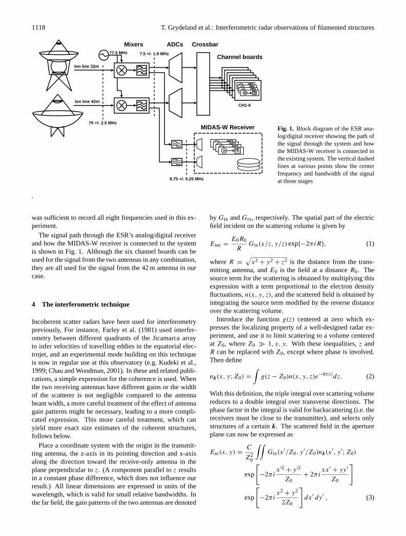
Fig. 1. Block diagram of the ESR ana-log/digital receiver showing the path ofthe signal through the system and howthe MIDAS-W receiver is connected tothe existing system. The vertical dashedlines at various points show the centerfrequency and bandwidth of the signalat those stages

.

was sufficient to record all eight frequencies used in this ex-periment.

The signal path through the ESR’s analog/digital receiverand how the MIDAS-W receiver is connected to the systemis shown in Fig. 1. Although the six channel boards can beused for the signal from the two antennas in any combination,they are all used for the signal from the 42 m antenna in ourcase.

4 The interferometric technique

Incoherent scatter radars have been used for interferometrypreviously, For instance, Farley et al. (1981) used interfer-ometry between different quadrants of the Jicamarca arrayto infer velocities of travelling eddies in the equatorial elec-trojet, and an experimental mode building on this techniqueis now in regular use at this observatory (e.g. Kudeki et al.,1999; Chau and Woodman, 2001). In these and related publi-cations, a simple expression for the coherence is used. Whenthe two receiving antennas have different gains or the widthof the scatterer is not negligible compared to the antennabeam width, a more careful treatment of the effect of antennagain patterns might be necessary, leading to a more compli-cated expression. This more careful treatment, which canyield more exact size estimates of the coherent structures,follows below.

Place a coordinate system with the origin in the transmit-ting antenna, the z-axis in its pointing direction and x-axisalong the direction toward the receive-only antenna in theplane perpendicular toz. (A component parallel toz resultsin a constant phase difference, which does not influence ourresult.) All linear dimensions are expressed in units of thewavelength, which is valid for small relative bandwidths. Inthe far field, the gain patterns of the two antennas are denoted

by Gtx andGrx, respectively. The spatial part of the electricfield incident on the scattering volume is given by

Einc =E0R0

RGtx(x/z, y/z) exp{−2πiR}, (1)

whereR =

√x2 + y2 + z2 is the distance from the trans-

mitting antenna, andE0 is the field at a distanceR0. Thesource term for the scattering is obtained by multiplying thisexpression with a term proportional to the electron densityfluctuations,n(x, y, z), and the scattered field is obtained byintegrating the source term modified by the reverse distanceover the scattering volume.

Introduce the functiong(z) centered at zero which ex-presses the localizing property of a well-designed radar ex-periment, and use it to limit scattering to a volume centeredat Z0, whereZ0 � 1, x, y. With these inequalities,z andR can be replaced withZ0, except where phase is involved.Then define

nk(x, y; Z0) =

∫g(z − Z0)n(x, y, z)e−4πizdz. (2)

With this definition, the triple integral over scattering volumereduces to a double integral over transverse directions. Thephase factor in the integral is valid for backscattering (i.e. thereceivers must be close to the transmitter), and selects onlystructures of a certaink. The scattered field in the apertureplane can now be expressed as

Esc(x, y) =C

Z20

∫∫Gtx(x

′/Z0, y′/Z0)nk(x

′, y′;Z0)

exp

[−2πi

x′2+ y′2

Z0+ 2πi

xx′+ yy′

Z0

]

exp

[−2πi

x2+ y2

2Z0

]dx′ dy′ , (3)


where the constantC describes the scattering strength of themedium and includes among others the scattering cross sec-tion of an electron and the factorE0R0.

The received signals in an arbitrary antenna on the groundcan now be found by integrating this field over the antennaaperture, which, in the far field approximation, is equivalentto multiplying the expression under the integrals with the re-ceiving antenna pattern and taking the phase from its centre.

The received signal in the transmitting antenna is given by

ftx =C

Z20

∫∫nk(x, y; Z0)G

2txe

−2πi(x2+y2)/Z0dx dy. (4)

And for the receive-only antenna, with gain patternGrx anddisplaced distance(x, y) = (A, 0),

frx =C

Z20

∫∫nk(x, y;Z0)GtxGrxe

−2πi(x2+y2−Ax)/Z0dx dy, (5)

where the constant phase factore−πiA2/Z0 has been dis-carded.

From expressions (4) and (5), form the cross-product andensemble average, which gives an expression for the complexspatial cross-correlation of the scattering received in the twoantennas. Assume homogeneity for the spatial correlations,⟨nk(x, y; Z0)n

∗

k(x′, y′

; Z0)⟩ ⟨

|1n|2⟩δ(x − x′)δ(y − y′), (6)

introduce the angles of integrationθx = x/Z0, θy = y/Z0,and obtain⟨ftxf

∗rx

⟩=

C2

Z20

∫∫ ⟨|1n|

2(θx, θy)⟩e−2πiAθx

×Gtx(θx, θy)3 Grx(θx, θy) dθxdθy . (7)

Assuming for mathematical convenience Gaussian gain pat-terns for the two antennas,

Gtx,rx(θx, θy) = exp

[−

θ2x + θ2

y

2σtx,rx

], (8)

and likewise that a discrete scatterer centered at(θxo, θyo)

has a Gaussian shape with unequal widths in the x- and y-directions,σx andσy , respectively,⟨|1n(θx, θy)|

2⟩= exp

[−

(θx − θxo)2

2σ 2x

−(θy − θyo)

2

2σ 2y

], (9)

the integrals in (7) can be evaluated to obtain

⟨ftxf

∗rx

⟩=

C2

Z20

exp

[−

1

2

D2x

62

θ2xo

σ 2x

−1

2

D2y

62

θ2yo

σ 2y

]

× exp

[−

1

2(2πA)2D2

x

]e−2πiAθxoD

2x/σ2

x , (10)

where

1

62=

3

σ 2tx

+1

σ 2rx

,1

D2x,y

=1

62+

1

σ 2x,y

.

0 0.1 0.2 0.3 0.4 0.5 0.6 0.7 0.80

0.2

0.4

0.6

0.8

1

structure size/fringe size

cohe

renc

e

Comparison of simple and detailed interferometric models

detailedsimple

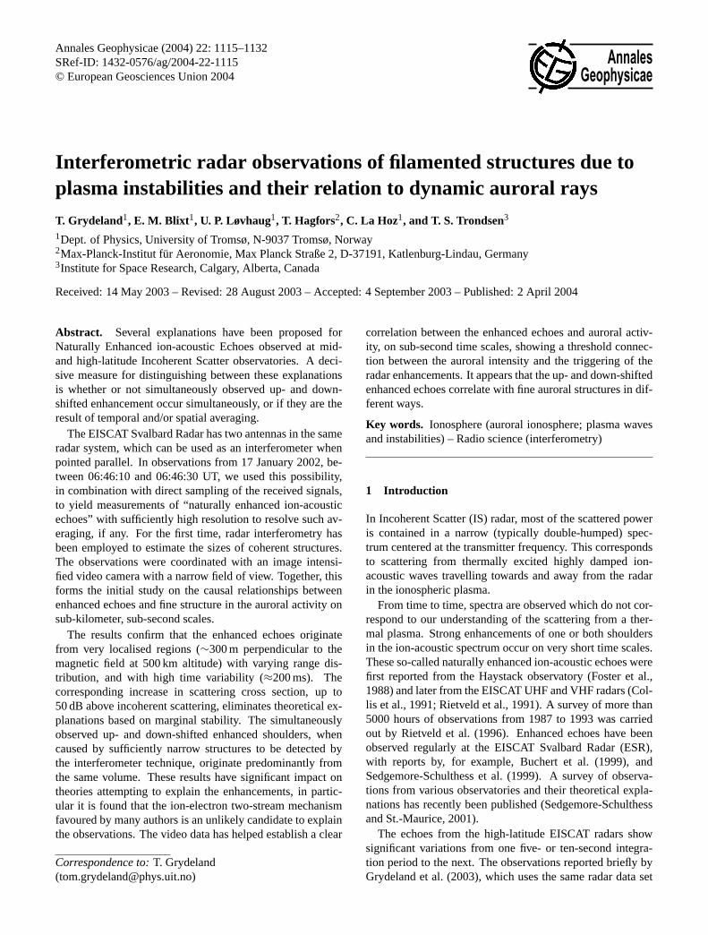
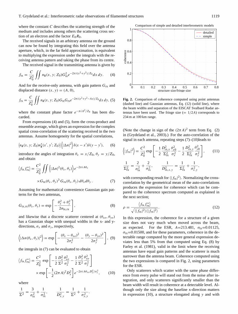
Fig. 2. Comparison of coherence computed using point antennas(dashed line) and Gaussian antennas, Eq. (12) (solid line), wherethe beam widths and separation of the EISCAT Svalbard Radar an-tennas have been used. The fringe size (= 1/2A) corresponds to234 m at 100 km range.

(Note the change in sign of the(2πA)2 term from Eq. (2)in (Grydeland et al., 2003).) For the auto-correlation of thesignal in each antenna, repeating steps (7)–(10)leads to⟨|frx|

2⟩=

C2

Z20

exp

[−

1

2

D2rx,x

62rx

θ2x0

σ 2x

−1

2

D2rx,y

62rx

θ2y0

σ 2y

], (11)

1

62rx

=2

σ 2tx

+2

σ 2rx

,1

D2rx,x,y

=1

62rx

+1

σ 2x,y

,

with corresponding result for〈|ftx|2〉. Normalizing the cross-

correlation by the geometrical mean of the auto-correlationsproduces the expression for coherence which can be com-pared to the coherence spectrum computed as explained inthe next section;

ρ =

⟨ftxf

∗rx

⟩√〈|ftx|

2〉〈|frx|2〉

. (12)

In this expression, the coherence for a structure of a givensize does not vary much when moved across the beam,as expected. For the ESR,A=213.481, σtx=0.01125,σrx=0.01500, and for these parameters, coherence in the de-tectable range computed by the more general expression de-viates less than 5% from that computed using Eq. (8) byFarley et al. (1981), valid in the limit where the receivingantennas have equal gain patterns and the scatterer is muchnarrower than the antenna beam. Coherence computed usingthe two expressions is compared in Fig. 2, using parametersfor the ESR.

Only scatterers which scatter with the same phase differ-ence from every pulse will stand out from the noise after in-tegration, and only scatterers significantly smaller than thebeam width will result in coherence at a detectable level. Al-though only the size along the baseline x-direction mattersin expression (10), a structure elongated alongy and with


z1*z0

* z2* z3

* z4*

w1

w2

w3

w4

w0

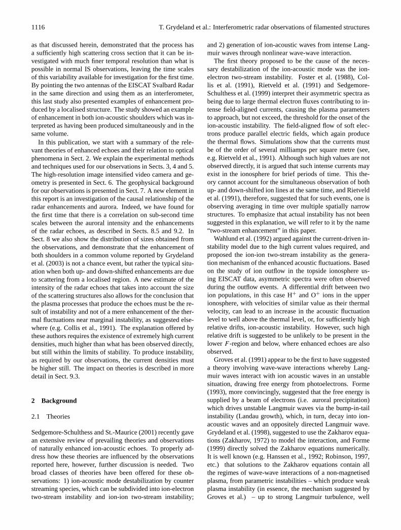
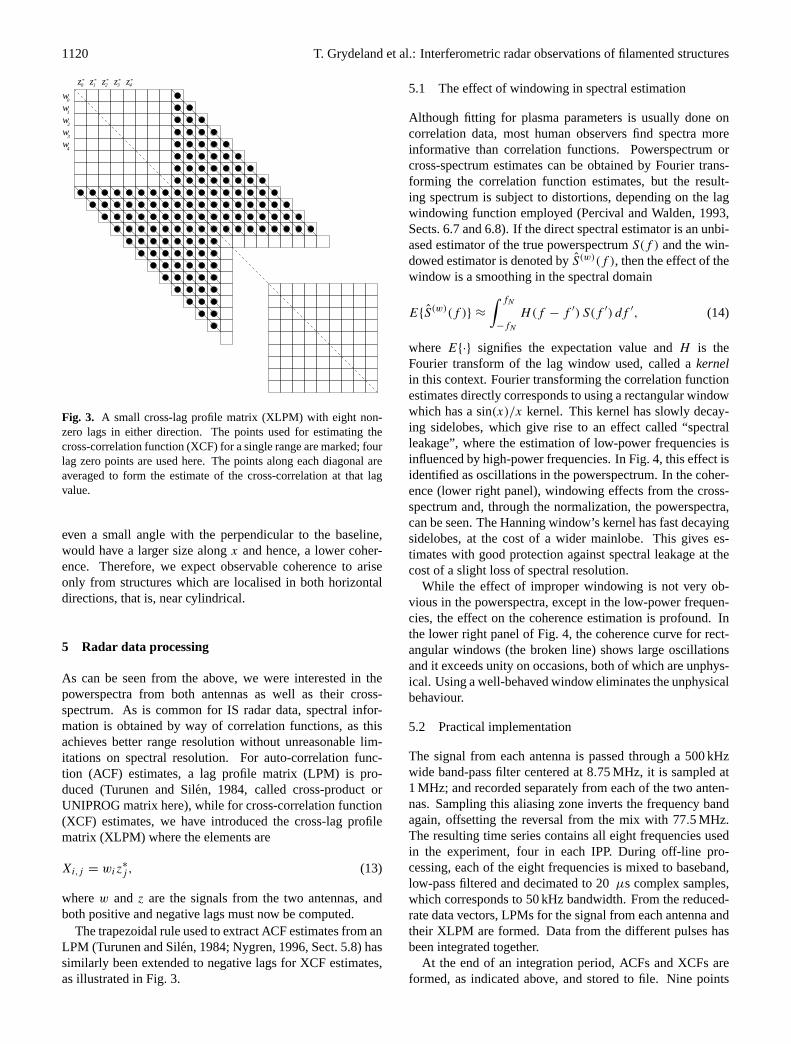
Fig. 3. A small cross-lag profile matrix (XLPM) with eight non-zero lags in either direction. The points used for estimating thecross-correlation function (XCF) for a single range are marked; fourlag zero points are used here. The points along each diagonal areaveraged to form the estimate of the cross-correlation at that lagvalue.

even a small angle with the perpendicular to the baseline,would have a larger size alongx and hence, a lower coher-ence. Therefore, we expect observable coherence to ariseonly from structures which are localised in both horizontaldirections, that is, near cylindrical.

5 Radar data processing

As can be seen from the above, we were interested in thepowerspectra from both antennas as well as their cross-spectrum. As is common for IS radar data, spectral infor-mation is obtained by way of correlation functions, as thisachieves better range resolution without unreasonable lim-itations on spectral resolution. For auto-correlation func-tion (ACF) estimates, a lag profile matrix (LPM) is pro-duced (Turunen and Silen, 1984, called cross-product orUNIPROG matrix here), while for cross-correlation function(XCF) estimates, we have introduced the cross-lag profilematrix (XLPM) where the elements are

Xi,j = wiz∗

j , (13)

wherew and z are the signals from the two antennas, andboth positive and negative lags must now be computed.

The trapezoidal rule used to extract ACF estimates from anLPM (Turunen and Silen, 1984; Nygren, 1996, Sect. 5.8) hassimilarly been extended to negative lags for XCF estimates,as illustrated in Fig. 3.

5.1 The effect of windowing in spectral estimation

Although fitting for plasma parameters is usually done oncorrelation data, most human observers find spectra moreinformative than correlation functions. Powerspectrum orcross-spectrum estimates can be obtained by Fourier trans-forming the correlation function estimates, but the result-ing spectrum is subject to distortions, depending on the lagwindowing function employed (Percival and Walden, 1993,Sects. 6.7 and 6.8). If the direct spectral estimator is an unbi-ased estimator of the true powerspectrumS(f ) and the win-dowed estimator is denoted byS(w)(f ), then the effect of thewindow is a smoothing in the spectral domain

E{S(w)(f )} ≈

∫ fN

−fN

H(f − f ′) S(f ′) df ′, (14)

where E{·} signifies the expectation value andH is theFourier transform of the lag window used, called akernelin this context. Fourier transforming the correlation functionestimates directly corresponds to using a rectangular windowwhich has a sin(x)/x kernel. This kernel has slowly decay-ing sidelobes, which give rise to an effect called “spectralleakage”, where the estimation of low-power frequencies isinfluenced by high-power frequencies. In Fig. 4, this effect isidentified as oscillations in the powerspectrum. In the coher-ence (lower right panel), windowing effects from the cross-spectrum and, through the normalization, the powerspectra,can be seen. The Hanning window’s kernel has fast decayingsidelobes, at the cost of a wider mainlobe. This gives es-timates with good protection against spectral leakage at thecost of a slight loss of spectral resolution.

While the effect of improper windowing is not very ob-vious in the powerspectra, except in the low-power frequen-cies, the effect on the coherence estimation is profound. Inthe lower right panel of Fig. 4, the coherence curve for rect-angular windows (the broken line) shows large oscillationsand it exceeds unity on occasions, both of which are unphys-ical. Using a well-behaved window eliminates the unphysicalbehaviour.

5.2 Practical implementation

The signal from each antenna is passed through a 500 kHzwide band-pass filter centered at 8.75 MHz, it is sampled at1 MHz; and recorded separately from each of the two anten-nas. Sampling this aliasing zone inverts the frequency bandagain, offsetting the reversal from the mix with 77.5 MHz.The resulting time series contains all eight frequencies usedin the experiment, four in each IPP. During off-line pro-cessing, each of the eight frequencies is mixed to baseband,low-pass filtered and decimated to 20µs complex samples,which corresponds to 50 kHz bandwidth. From the reduced-rate data vectors, LPMs for the signal from each antenna andtheir XLPM are formed. Data from the different pulses hasbeen integrated together.

At the end of an integration period, ACFs and XCFs areformed, as indicated above, and stored to file. Nine points


0 90 180 270 360−4

−2

0

2

4

6ACF estimates, 42m antenna

lag [µs]−360 −180 0 180 360−2

−1

0

1

2XCF estimates

lag [µs]

−20 −10 0 10 20−10

0

10

20Powerspectrum [dB]

frequency [kHz]−20 −10 0 10 20

0.25

0.5

0.75

−20 −10 0 10 20

−pi/2

0

pi/2

Coherence and phase

frequency [kHz]

2002−01−[email protected], 733 km, deltaphi=0

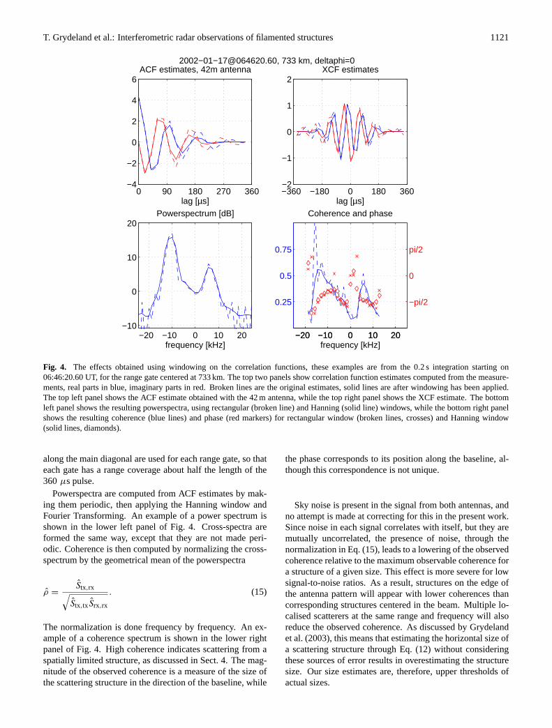
Fig. 4. The effects obtained using windowing on the correlation functions, these examples are from the 0.2 s integration starting on06:46:20.60 UT, for the range gate centered at 733 km. The top two panels show correlation function estimates computed from the measure-ments, real parts in blue, imaginary parts in red. Broken lines are the original estimates, solid lines are after windowing has been applied.The top left panel shows the ACF estimate obtained with the 42 m antenna, while the top right panel shows the XCF estimate. The bottomleft panel shows the resulting powerspectra, using rectangular (broken line) and Hanning (solid line) windows, while the bottom right panelshows the resulting coherence (blue lines) and phase (red markers) for rectangular window (broken lines, crosses) and Hanning window(solid lines, diamonds).

along the main diagonal are used for each range gate, so thateach gate has a range coverage about half the length of the360 µs pulse.

Powerspectra are computed from ACF estimates by mak-ing them periodic, then applying the Hanning window andFourier Transforming. An example of a power spectrum isshown in the lower left panel of Fig. 4. Cross-spectra areformed the same way, except that they are not made peri-odic. Coherence is then computed by normalizing the cross-spectrum by the geometrical mean of the powerspectra

ρ =Stx,rx√

Stx,txSrx,rx

. (15)

The normalization is done frequency by frequency. An ex-ample of a coherence spectrum is shown in the lower rightpanel of Fig. 4. High coherence indicates scattering from aspatially limited structure, as discussed in Sect. 4. The mag-nitude of the observed coherence is a measure of the size ofthe scattering structure in the direction of the baseline, while

the phase corresponds to its position along the baseline, al-though this correspondence is not unique.

Sky noise is present in the signal from both antennas, andno attempt is made at correcting for this in the present work.Since noise in each signal correlates with itself, but they aremutually uncorrelated, the presence of noise, through thenormalization in Eq. (15), leads to a lowering of the observedcoherence relative to the maximum observable coherence fora structure of a given size. This effect is more severe for lowsignal-to-noise ratios. As a result, structures on the edge ofthe antenna pattern will appear with lower coherences thancorresponding structures centered in the beam. Multiple lo-calised scatterers at the same range and frequency will alsoreduce the observed coherence. As discussed by Grydelandet al. (2003), this means that estimating the horizontal size ofa scattering structure through Eq. (12) without consideringthese sources of error results in overestimating the structuresize. Our size estimates are, therefore, upper thresholds ofactual sizes.


0 100 200 300 400 500 6000

100

200

300

400

Line a.

Line b.

b1

b2

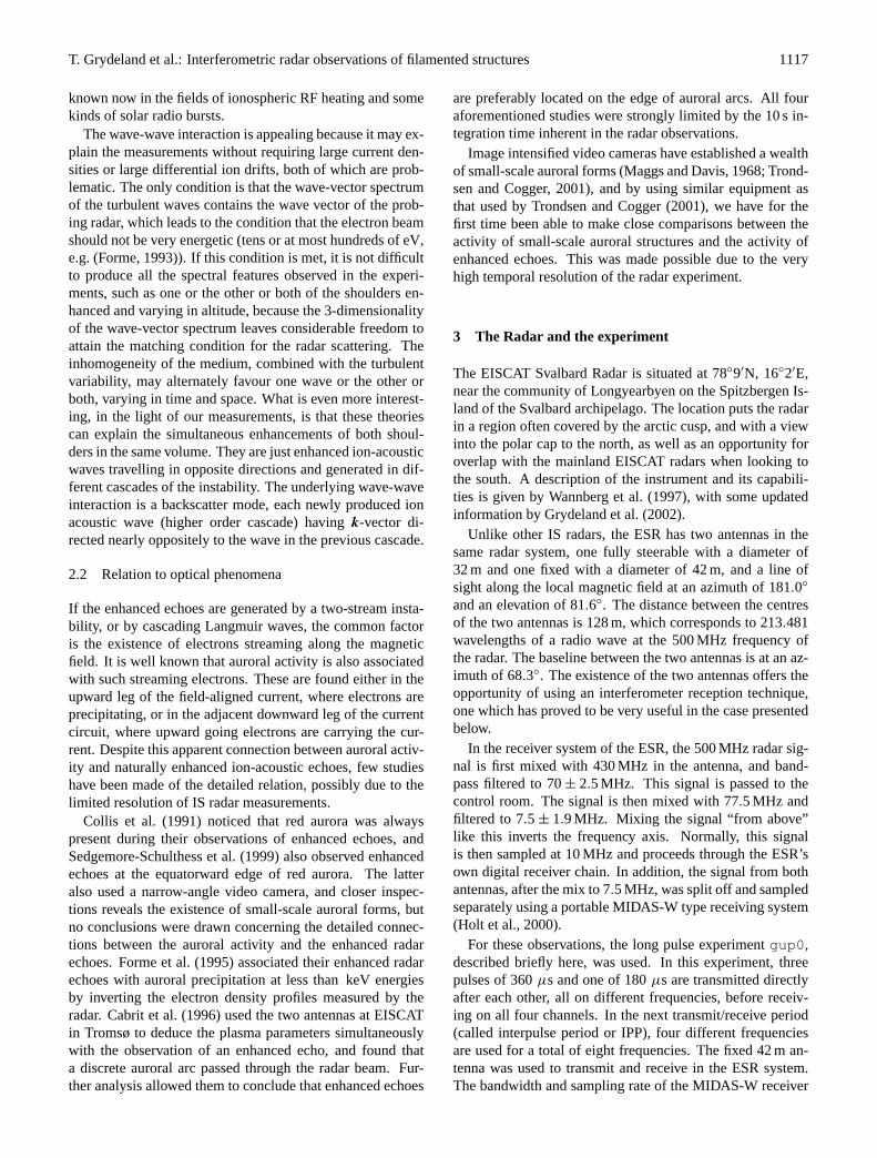
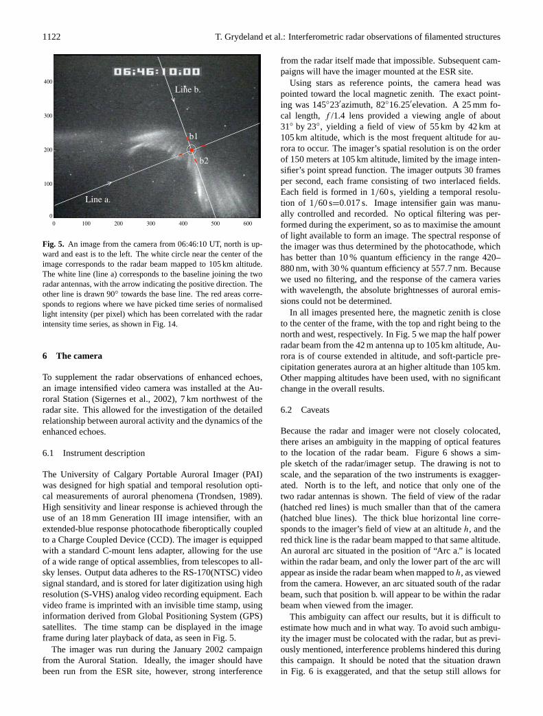
Fig. 5. An image from the camera from 06:46:10 UT, north is up-ward and east is to the left. The white circle near the center of theimage corresponds to the radar beam mapped to 105 km altitude.The white line (line a) corresponds to the baseline joining the tworadar antennas, with the arrow indicating the positive direction. Theother line is drawn 90◦ towards the base line. The red areas corre-sponds to regions where we have picked time series of normalisedlight intensity (per pixel) which has been correlated with the radarintensity time series, as shown in Fig. 14.

6 The camera

To supplement the radar observations of enhanced echoes,an image intensified video camera was installed at the Au-roral Station (Sigernes et al., 2002), 7 km northwest of theradar site. This allowed for the investigation of the detailedrelationship between auroral activity and the dynamics of theenhanced echoes.

6.1 Instrument description

The University of Calgary Portable Auroral Imager (PAI)was designed for high spatial and temporal resolution opti-cal measurements of auroral phenomena (Trondsen, 1989).High sensitivity and linear response is achieved through theuse of an 18 mm Generation III image intensifier, with anextended-blue response photocathode fiberoptically coupledto a Charge Coupled Device (CCD). The imager is equippedwith a standard C-mount lens adapter, allowing for the useof a wide range of optical assemblies, from telescopes to all-sky lenses. Output data adheres to the RS-170(NTSC) videosignal standard, and is stored for later digitization using highresolution (S-VHS) analog video recording equipment. Eachvideo frame is imprinted with an invisible time stamp, usinginformation derived from Global Positioning System (GPS)satellites. The time stamp can be displayed in the imageframe during later playback of data, as seen in Fig. 5.

The imager was run during the January 2002 campaignfrom the Auroral Station. Ideally, the imager should havebeen run from the ESR site, however, strong interference

from the radar itself made that impossible. Subsequent cam-paigns will have the imager mounted at the ESR site.

Using stars as reference points, the camera head waspointed toward the local magnetic zenith. The exact point-ing was 145◦23′azimuth, 82◦16.25′elevation. A 25 mm fo-cal length,f /1.4 lens provided a viewing angle of about31◦ by 23◦, yielding a field of view of 55 km by 42 km at105 km altitude, which is the most frequent altitude for au-rora to occur. The imager’s spatial resolution is on the orderof 150 meters at 105 km altitude, limited by the image inten-sifier’s point spread function. The imager outputs 30 framesper second, each frame consisting of two interlaced fields.Each field is formed in 1/60 s, yielding a temporal resolu-tion of 1/60 s=0.017 s. Image intensifier gain was manu-ally controlled and recorded. No optical filtering was per-formed during the experiment, so as to maximise the amountof light available to form an image. The spectral response ofthe imager was thus determined by the photocathode, whichhas better than 10 % quantum efficiency in the range 420–880 nm, with 30 % quantum efficiency at 557.7 nm. Becausewe used no filtering, and the response of the camera varieswith wavelength, the absolute brightnesses of auroral emis-sions could not be determined.

In all images presented here, the magnetic zenith is closeto the center of the frame, with the top and right being to thenorth and west, respectively. In Fig. 5 we map the half powerradar beam from the 42 m antenna up to 105 km altitude, Au-rora is of course extended in altitude, and soft-particle pre-cipitation generates aurora at an higher altitude than 105 km.Other mapping altitudes have been used, with no significantchange in the overall results.

6.2 Caveats

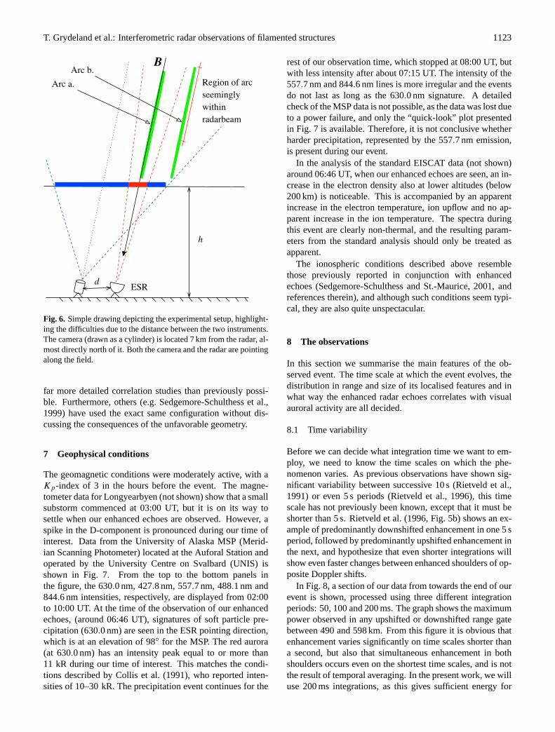
Because the radar and imager were not closely colocated,there arises an ambiguity in the mapping of optical featuresto the location of the radar beam. Figure 6 shows a sim-ple sketch of the radar/imager setup. The drawing is not toscale, and the separation of the two instruments is exagger-ated. North is to the left, and notice that only one of thetwo radar antennas is shown. The field of view of the radar(hatched red lines) is much smaller than that of the camera(hatched blue lines). The thick blue horizontal line corre-sponds to the imager’s field of view at an altitudeh, and thered thick line is the radar beam mapped to that same altitude.An auroral arc situated in the position of “Arc a.” is locatedwithin the radar beam, and only the lower part of the arc willappear as inside the radar beam when mapped toh, as viewedfrom the camera. However, an arc situated south of the radarbeam, such that position b. will appear to be within the radarbeam when viewed from the imager.

This ambiguity can affect our results, but it is difficult toestimate how much and in what way. To avoid such ambigu-ity the imager must be colocated with the radar, but as previ-ously mentioned, interference problems hindered this duringthis campaign. It should be noted that the situation drawnin Fig. 6 is exaggerated, and that the setup still allows for


BArc b.

Region of arcseeminglywithinradarbeam

h

d

Arc a.

ESR

Fig. 6. Simple drawing depicting the experimental setup, highlight-ing the difficulties due to the distance between the two instruments.The camera (drawn as a cylinder) is located 7 km from the radar, al-most directly north of it. Both the camera and the radar are pointingalong the field.

far more detailed correlation studies than previously possi-ble. Furthermore, others (e.g. Sedgemore-Schulthess et al.,1999) have used the exact same configuration without dis-cussing the consequences of the unfavorable geometry.

7 Geophysical conditions

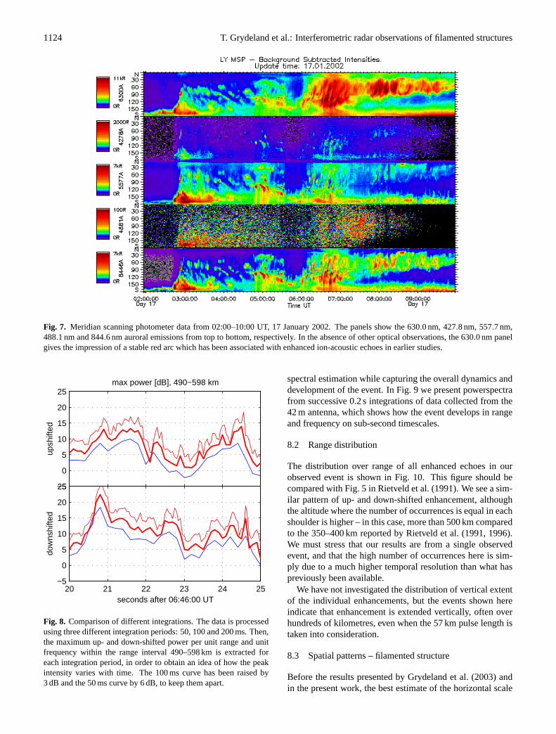
The geomagnetic conditions were moderately active, with aKp-index of 3 in the hours before the event. The magne-tometer data for Longyearbyen (not shown) show that a smallsubstorm commenced at 03:00 UT, but it is on its way tosettle when our enhanced echoes are observed. However, aspike in the D-component is pronounced during our time ofinterest. Data from the University of Alaska MSP (Merid-ian Scanning Photometer) located at the Auforal Station andoperated by the University Centre on Svalbard (UNIS) isshown in Fig. 7. From the top to the bottom panels inthe figure, the 630.0 nm, 427.8 nm, 557.7 nm, 488.1 nm and844.6 nm intensities, respectively, are displayed from 02:00to 10:00 UT. At the time of the observation of our enhancedechoes, (around 06:46 UT), signatures of soft particle pre-cipitation (630.0 nm) are seen in the ESR pointing direction,which is at an elevation of 98◦ for the MSP. The red aurora(at 630.0 nm) has an intensity peak equal to or more than11 kR during our time of interest. This matches the condi-tions described by Collis et al. (1991), who reported inten-sities of 10–30 kR. The precipitation event continues for the

rest of our observation time, which stopped at 08:00 UT, butwith less intensity after about 07:15 UT. The intensity of the557.7 nm and 844.6 nm lines is more irregular and the eventsdo not last as long as the 630.0 nm signature. A detailedcheck of the MSP data is not possible, as the data was lost dueto a power failure, and only the “quick-look” plot presentedin Fig. 7 is available. Therefore, it is not conclusive whetherharder precipitation, represented by the 557.7 nm emission,is present during our event.

In the analysis of the standard EISCAT data (not shown)around 06:46 UT, when our enhanced echoes are seen, an in-crease in the electron density also at lower altitudes (below200 km) is noticeable. This is accompanied by an apparentincrease in the electron temperature, ion upflow and no ap-parent increase in the ion temperature. The spectra duringthis event are clearly non-thermal, and the resulting param-eters from the standard analysis should only be treated asapparent.

The ionospheric conditions described above resemblethose previously reported in conjunction with enhancedechoes (Sedgemore-Schulthess and St.-Maurice, 2001, andreferences therein), and although such conditions seem typi-cal, they are also quite unspectacular.

8 The observations

In this section we summarise the main features of the ob-served event. The time scale at which the event evolves, thedistribution in range and size of its localised features and inwhat way the enhanced radar echoes correlates with visualauroral activity are all decided.

8.1 Time variability

Before we can decide what integration time we want to em-ploy, we need to know the time scales on which the phe-nomenon varies. As previous observations have shown sig-nificant variability between successive 10 s (Rietveld et al.,1991) or even 5 s periods (Rietveld et al., 1996), this timescale has not previously been known, except that it must beshorter than 5 s. Rietveld et al. (1996, Fig. 5b) shows an ex-ample of predominantly downshifted enhancement in one 5 speriod, followed by predominantly upshifted enhancement inthe next, and hypothesize that even shorter integrations willshow even faster changes between enhanced shoulders of op-posite Doppler shifts.

In Fig. 8, a section of our data from towards the end of ourevent is shown, processed using three different integrationperiods: 50, 100 and 200 ms. The graph shows the maximumpower observed in any upshifted or downshifted range gatebetween 490 and 598 km. From this figure it is obvious thatenhancement varies significantly on time scales shorter thana second, but also that simultaneous enhancement in bothshoulders occurs even on the shortest time scales, and is notthe result of temporal averaging. In the present work, we willuse 200 ms integrations, as this gives sufficient energy for


Fig. 7. Meridian scanning photometer data from 02:00–10:00 UT, 17 January 2002. The panels show the 630.0 nm, 427.8 nm, 557.7 nm,488.1 nm and 844.6 nm auroral emissions from top to bottom, respectively. In the absence of other optical observations, the 630.0 nm panelgives the impression of a stable red arc which has been associated with enhanced ion-acoustic echoes in earlier studies.

20 21 22 23 24 25−5

0

5

10

15

20

25

dow

nshi

fted

seconds after 06:46:00 UT

−5

0

5

10

15

20

25

upsh

ifted

max power [dB], 490−598 km

Fig. 8. Comparison of different integrations. The data is processedusing three different integration periods: 50, 100 and 200 ms. Then,the maximum up- and down-shifted power per unit range and unitfrequency within the range interval 490–598 km is extracted foreach integration period, in order to obtain an idea of how the peakintensity varies with time. The 100 ms curve has been raised by3 dB and the 50 ms curve by 6 dB, to keep them apart.

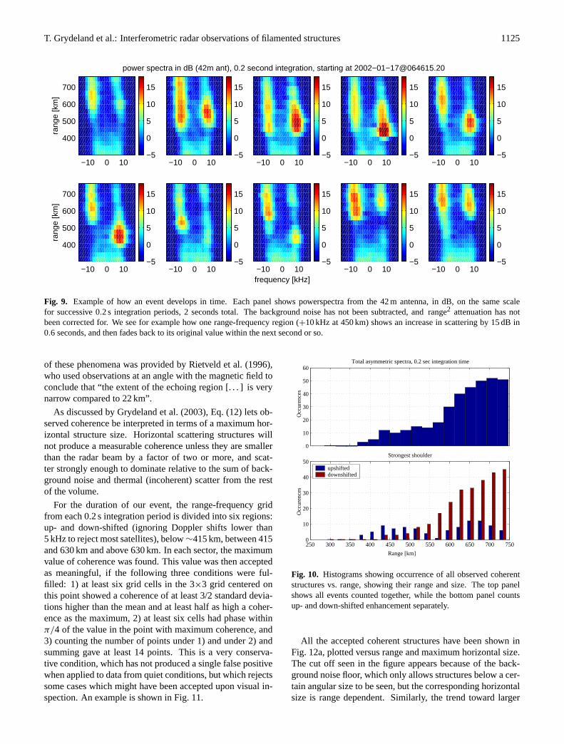
spectral estimation while capturing the overall dynamics anddevelopment of the event. In Fig. 9 we present powerspectrafrom successive 0.2 s integrations of data collected from the42 m antenna, which shows how the event develops in rangeand frequency on sub-second timescales.

8.2 Range distribution

The distribution over range of all enhanced echoes in ourobserved event is shown in Fig. 10. This figure should becompared with Fig. 5 in Rietveld et al. (1991). We see a sim-ilar pattern of up- and down-shifted enhancement, althoughthe altitude where the number of occurrences is equal in eachshoulder is higher – in this case, more than 500 km comparedto the 350–400 km reported by Rietveld et al. (1991, 1996).We must stress that our results are from a single observedevent, and that the high number of occurrences here is sim-ply due to a much higher temporal resolution than what haspreviously been available.

We have not investigated the distribution of vertical extentof the individual enhancements, but the events shown hereindicate that enhancement is extended vertically, often overhundreds of kilometres, even when the 57 km pulse length istaken into consideration.

8.3 Spatial patterns – filamented structure

Before the results presented by Grydeland et al. (2003) andin the present work, the best estimate of the horizontal scale


−5

0

5

10

15

−10 0 10

400

500

600

700

rang

e [k

m]

−5

0

5

10

15

−10 0 10−5

0

5

10

15

−10 0 10

power spectra in dB (42m ant), 0.2 second integration, starting at 2002−01−[email protected]

−5

0

5

10

15

−10 0 10−5

0

5

10

15

−10 0 10

−5

0

5

10

15

−10 0 10

400

500

600

700

rang

e [k

m]

−5

0

5

10

15

−10 0 10−5

0

5

10

15

−10 0 10frequency [kHz]

−5

0

5

10

15

−10 0 10−5

0

5

10

15

−10 0 10

Fig. 9. Example of how an event develops in time. Each panel shows powerspectra from the 42 m antenna, in dB, on the same scalefor successive 0.2 s integration periods, 2 seconds total. The background noise has not been subtracted, and range2 attenuation has notbeen corrected for. We see for example how one range-frequency region (+10 kHz at 450 km) shows an increase in scattering by 15 dB in0.6 seconds, and then fades back to its original value within the next second or so.

of these phenomena was provided by Rietveld et al. (1996),who used observations at an angle with the magnetic field toconclude that “the extent of the echoing region [. . . ] is verynarrow compared to 22 km”.

As discussed by Grydeland et al. (2003), Eq. (12) lets ob-served coherence be interpreted in terms of a maximum hor-izontal structure size. Horizontal scattering structures willnot produce a measurable coherence unless they are smallerthan the radar beam by a factor of two or more, and scat-ter strongly enough to dominate relative to the sum of back-ground noise and thermal (incoherent) scatter from the restof the volume.

For the duration of our event, the range-frequency gridfrom each 0.2 s integration period is divided into six regions:up- and down-shifted (ignoring Doppler shifts lower than5 kHz to reject most satellites), below∼415 km, between 415and 630 km and above 630 km. In each sector, the maximumvalue of coherence was found. This value was then acceptedas meaningful, if the following three conditions were ful-filled: 1) at least six grid cells in the 3×3 grid centered onthis point showed a coherence of at least 3/2 standard devia-tions higher than the mean and at least half as high a coher-ence as the maximum, 2) at least six cells had phase withinπ/4 of the value in the point with maximum coherence, and3) counting the number of points under 1) and under 2) andsumming gave at least 14 points. This is a very conserva-tive condition, which has not produced a single false positivewhen applied to data from quiet conditions, but which rejectssome cases which might have been accepted upon visual in-spection. An example is shown in Fig. 11.

0

10

20

30

40

50

60Total asymmetric spectra, 0.2 sec integration time

Occ

uren

ces

250 300 350 400 450 500 550 600 650 700 7500

10

20

30

40

50Strongest shoulder

Range [km]

Occ

uren

ces

upshifted downshifted

Fig. 10. Histograms showing occurrence of all observed coherentstructures vs. range, showing their range and size. The top panelshows all events counted together, while the bottom panel countsup- and down-shifted enhancement separately.

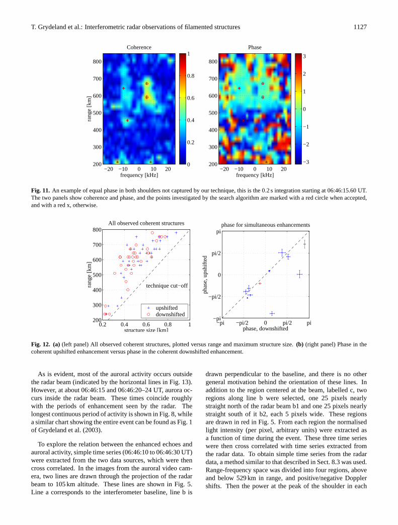
All the accepted coherent structures have been shown inFig. 12a, plotted versus range and maximum horizontal size.The cut off seen in the figure appears because of the back-ground noise floor, which only allows structures below a cer-tain angular size to be seen, but the corresponding horizontalsize is range dependent. Similarly, the trend toward larger


size structures at longer ranges might be an effect of a lowersignal-to-noise ratio, resulting in lower coherence.

As the sizes plotted in Fig. 12a are upper bounds, weshould be careful not to try a too detailed interpretation. Afew observations can still be made. First, there is no obvi-ous difference between up- and down-shifted enhancementsin their distribution in size and range. Second, there is acomparable number of up- and down-shifted enhancementsat longer ranges, while Fig. 10 shows larger numbers ofdownshifted enhancements at longer ranges. It might seemthat downshifted enhancement, while more common, is lesslikely to give rise to observable coherence.

As pointed out by Grydeland et al. (2003), the extremelylocalised scattering structures in these observations meanthat not only is the total scattering increased by a factorof 100 or so, but this increased scattering originates fromas little as 0.3% of the total beam volume, possibly evenless. These authors conclude that the scattering cross sectionwithin the filament must, therefore, be 4–5 orders of magni-tude above thermal levels.

We want to add the observation that observable coherenceis in itself an indication that our time resolution is sufficient.If our enhanced scattering were caused by several extremelyshort-lived structures (simultaneous or not, coherent or not)within an integration, these would have randomly distributedphases, and would not ordinarily result in an observable co-herence at longer integrations.

8.4 Phase as an indication of horizontal position

The cross-spectrum phase due to a localised scatterer de-pends on its position along the baseline, as indicated byEq. (10), and is computed frequency by frequency. As a re-sult, when the coherence indicates a localised scatterer at agiven range and frequency, the phase in this range-frequencyregion can be used to determine the position of the scattererin one spatial dimension, with some limitations discussed inSect. 9.1. This information is used to decide whether simul-taneous enhancements in up- and down-shifted shoulders oc-cur in the same volume; therefore, from the coherent casesshown in Fig. 12a, those where an upshifted and downshiftedcoherent enhancement was seen within 100 km of range ofeach other in the same 0.2 s integration were selected. Forthese cases, the phase in the upshifted enhancement (φ+) isplotted against the phase in the downshifted enhancement(φ−) in Fig. 12b. The error bars indicate one standard de-viation of phase in the 3×3 region centered on the point ofhighest coherence.

The selection criteria used for coherent echoes are quitestrict. Furthermore, up- and down-shifted enhancements areconsidered separately, so occasionally one shoulder or theother is not accepted by the algorithm, although the patternis quite obvious to a human observer.

Another feature sometimes seen is phase varying linearlywith range, consistent with a scatterer located on a field linewith its foot-point outside the antenna. If, in such a situ-ation, the search algorithm finds points at slightly different

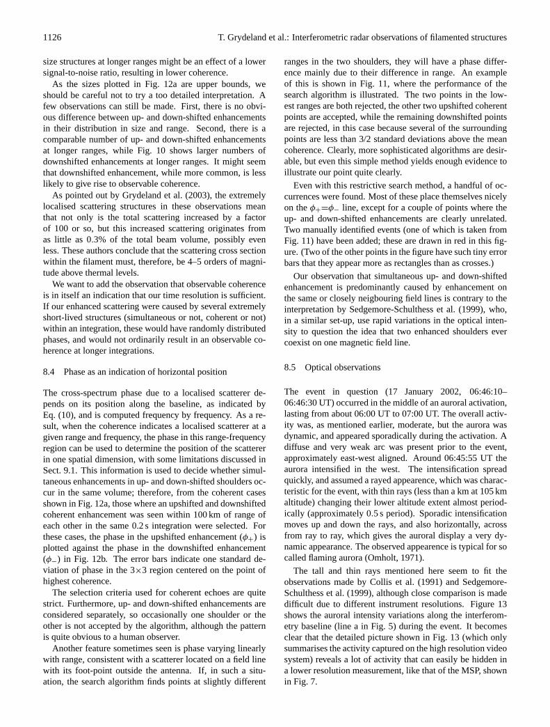
ranges in the two shoulders, they will have a phase differ-ence mainly due to their difference in range. An exampleof this is shown in Fig. 11, where the performance of thesearch algorithm is illustrated. The two points in the low-est ranges are both rejected, the other two upshifted coherentpoints are accepted, while the remaining downshifted pointsare rejected, in this case because several of the surroundingpoints are less than 3/2 standard deviations above the meancoherence. Clearly, more sophisticated algorithms are desir-able, but even this simple method yields enough evidence toillustrate our point quite clearly.

Even with this restrictive search method, a handful of oc-currences were found. Most of these place themselves nicelyon theφ+=φ− line, except for a couple of points where theup- and down-shifted enhancements are clearly unrelated.Two manually identified events (one of which is taken fromFig. 11) have been added; these are drawn in red in this fig-ure. (Two of the other points in the figure have such tiny errorbars that they appear more as rectangles than as crosses.)

Our observation that simultaneous up- and down-shiftedenhancement is predominantly caused by enhancement onthe same or closely neigbouring field lines is contrary to theinterpretation by Sedgemore-Schulthess et al. (1999), who,in a similar set-up, use rapid variations in the optical inten-sity to question the idea that two enhanced shoulders evercoexist on one magnetic field line.

8.5 Optical observations

The event in question (17 January 2002, 06:46:10–06:46:30 UT) occurred in the middle of an auroral activation,lasting from about 06:00 UT to 07:00 UT. The overall activ-ity was, as mentioned earlier, moderate, but the aurora wasdynamic, and appeared sporadically during the activation. Adiffuse and very weak arc was present prior to the event,approximately east-west aligned. Around 06:45:55 UT theaurora intensified in the west. The intensification spreadquickly, and assumed a rayed appearence, which was charac-teristic for the event, with thin rays (less than a km at 105 kmaltitude) changing their lower altitude extent almost period-ically (approximately 0.5 s period). Sporadic intensificationmoves up and down the rays, and also horizontally, acrossfrom ray to ray, which gives the auroral display a very dy-namic appearance. The observed appearence is typical for socalled flaming aurora (Omholt, 1971).

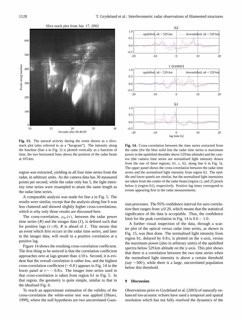
The tall and thin rays mentioned here seem to fit theobservations made by Collis et al. (1991) and Sedgemore-Schulthess et al. (1999), although close comparison is madedifficult due to different instrument resolutions. Figure 13shows the auroral intensity variations along the interferom-etry baseline (line a in Fig. 5) during the event. It becomesclear that the detailed picture shown in Fig. 13 (which onlysummarises the activity captured on the high resolution videosystem) reveals a lot of activity that can easily be hidden ina lower resolution measurement, like that of the MSP, shownin Fig. 7.


0

0.2

0.4

0.6

0.8

1

−3

−2

−1

0

1

2

3

frequency [kHz]

rang

e [k

m]

Coherence

−20 −10 0 10 20200

300

400

500

600

700

800

frequency [kHz]

Phase

−20 −10 0 10 20200

300

400

500

600

700

800

Fig. 11. An example of equal phase in both shoulders not captured by our technique, this is the 0.2 s integration starting at 06:46:15.60 UT.The two panels show coherence and phase, and the points investigated by the search algorithm are marked with a red circle when accepted,and with a red x, otherwise.

0.2 0.4 0.6 0.8 1200

300

400

500

600

700

800

technique cut−off

structure size [km]

rang

e [k

m]

All observed coherent structures

upshifted downshifted

−pi −pi/2 0 pi/2 pi−pi

−pi/2

0

pi/2

piphase for simultaneous enhancements

phase, downshifted

phas

e, u

pshi

fted

Fig. 12. (a)(left panel) All observed coherent structures, plotted versus range and maximum structure size.(b) (right panel) Phase in thecoherent upshifted enhancement versus phase in the coherent downshifted enhancement.

As is evident, most of the auroral activity occurs outsidethe radar beam (indicated by the horizontal lines in Fig. 13).However, at about 06:46:15 and 06:46:20–24 UT, aurora oc-curs inside the radar beam. These times coincide roughlywith the periods of enhancement seen by the radar. Thelongest continuous period of activity is shown in Fig. 8, whilea similar chart showing the entire event can be found as Fig. 1of Grydeland et al. (2003).

To explore the relation between the enhanced echoes andauroral activity, simple time series (06:46:10 to 06:46:30 UT)were extracted from the two data sources, which were thencross correlated. In the images from the auroral video cam-era, two lines are drawn through the projection of the radarbeam to 105 km altitude. These lines are shown in Fig. 5.Line a corresponds to the interferometer baseline, line b is

drawn perpendicular to the baseline, and there is no othergeneral motivation behind the orientation of these lines. Inaddition to the region centered at the beam, labelled c, tworegions along line b were selected, one 25 pixels nearlystraight north of the radar beam b1 and one 25 pixels nearlystraight south of it b2, each 5 pixels wide. These regionsare drawn in red in Fig. 5. From each region the normalisedlight intensity (per pixel, arbitrary units) were extracted asa function of time during the event. These three time serieswere then cross correlated with time series extracted fromthe radar data. To obtain simple time series from the radardata, a method similar to that described in Sect. 8.3 was used.Range-frequency space was divided into four regions, aboveand below 529 km in range, and positive/negative Dopplershifts. Then the power at the peak of the shoulder in each


Slice stack plot from Jan. 17, 2002

10 15 20 25 30Seconds after 06:46:00

0

100

200

300

400

500

600

Pixe

ls a

long

bas

elin

e

Fig. 13. The auroral activity during the event shown as a slice-stack plot (also referred to as a “keogram”). The intensity alongthe baseline (line a in Fig. 5) is plotted vertically as a function oftime, the two horizontal lines shows the position of the radar beamat 105 km.

region was extracted, yielding in all four time series from theradar, in arbitrary units. As the camera data has 30 measuredpoints per second, while the radar only has 5, the light inten-sity time series were resampled to attain the same length asthe radar time series.

A comparable analysis was made for line a in Fig. 5. Theresults were similar, except that the analysis along line b wasless cluttered and showed slightly higher cross-correlations,which is why only those results are discussed here.

The cross-correlation,ρRI (τ ), between the radar powertime series (R) and the imager data (I ), is defined such thatfor positive lags (τ>0), R is ahead ofI . This means thatan event which first occurs in the radar time series, and laterin the imager data, will result in a positive correlation at apositive lag.

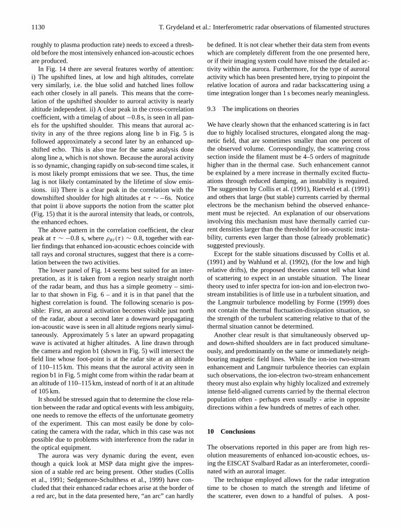
Figure 14 shows the resulting cross-correlation coefficient.The first thing to be noticed is that the correlation coefficientapproaches zero at lags greater than±10 s. Second, it is evi-dent that the overall correlation is rather low, and the highestcross-correlation coefficient (∼0.8 ) appears in Fig. 14 in thelower panel atτ∼ − 0.8 s. The imager time series used inthat cross-correlation is taken from region b1 in Fig. 5. Inthat region, the geometry is quite simple, similar to that inthe idealised Fig. 6.

To reach an approximate estimation of the validity of thecross-correlation the white-noise test was applied (Shiavi,1999), where the null hypothesis are two uncorrelated Gaus-

b2

-20 -10 0 10 20-0.5

0.0

0.5

1.0upshifted, alt > 529 km downshifted, alt > 529 km

c (center)

-20 -10 0 10 20-0.5

0.0

0.5

1.0upshifted, alt < 529 km downshifted, alt < 529 km

b1

-20 -10 0 10 20lag time [s]

-0.5

0.0

0.5

1.0

Fig. 14. Cross-correlation between the time series extracted fromthe radar (for the blue solid line the radar time series is maximumpower in the upshifted shoulder above 529 km altitude) and the cam-era (the camera time series are normalised light intensity drawnfrom the one of three regions; b1, c, b2, along line b in Fig. 5).The upper panel shows the cross-correlation between the radar timeseries and the normalised light intensity from region b2. The mid-dle and lower panels are similar, but the normalised light intensitiesare taken from the center of the radar beam (region c), and 25 pixelsbelow it (region b1), respectively. Positive lag times correspond toevents appearing first in the radar measurements.

sian processes. The 95% confidence interval for zero correla-tion then ranges from±0.20, which means that the statisticalsignificance of the data is acceptable. Thus, the confidencelimit for the peak correlation in Fig. 14 is 0.6 − 1.0 .

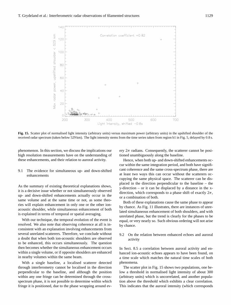
A further visual inspection of the data, through a scat-ter plot of the optical versus radar time series, as shown inFig. 15, was then done. The normalised light intensity fromregion b1, delayed by 0.8 s, is plotted on the x-axis, versusthe maximum power (also in arbitrary units) of the upshiftedspectra below 529 km altitude on the y-axis. This plot showsthat there is a correlation between the two time series whenthe normalised light intensity is above a certain threshold(say∼300 ), while there is a large, uncorrelated populationbelow this threshold.

9 Discussion

Observations prior to Grydeland et al. (2003) of naturally en-hanced ion-acoustic echoes have used a temporal and spatialresolution which has not fully resolved the dynamics of the


Fig. 15. Scatter plot of normalised light intensity (arbitrary units) versus maximum power (arbitrary units) in the upshifted shoulder of thereceived radar spectrum (taken below 529 km). The light intensity stems from the time series taken from region b1 in Fig. 5, delayed by 0.8 s.

phenomenon. In this section, we discuss the implications ourhigh resolution measurements have on the understanding ofthese enhancements, and their relation to auroral activity.

9.1 The evidence for simultaneous up- and down-shiftedenhancements

As the summary of existing theoretical explanations shows,it is a decisive issue whether or not simultaneously observedup- and down-shifted enhancements actually occur in thesame volume and at the same time or not, as some theo-ries will explain enhancement in only one or the other ion-acoustic shoulder, while simultaneous enhancement of bothis explained in terms of temporal or spatial averaging.

With our technique, the temporal evolution of the event isresolved. We also note that observing coherence at all is in-consistent with an explanation involving enhancements fromseveral unrelated scatterers. Therefore, we conclude withouta doubt that when both ion-acoustic shoulders are observedto be enhanced, this occurs simultaneously. The questionthen becomes whether the simultaneous enhancement occurswithin a single volume, or if opposite shoulders are enhancedin nearby volumes within the same beam.

With a single baseline, a localised scatterer detectedthrough interferometry cannot be localised in the directionperpendicular to the baseline, and although the positionwithin any one fringe can be determined through the cross-spectrum phase, it is not possible to determine within whichfringe it is positioned, due to the phase wrapping around ev-

ery 2π radians. Consequently, the scatterer cannot be posi-tioned unambiguously along the baseline.

Hence, when both up- and down-shifted enhancements oc-cur within the same integration period, and both have signifi-cant coherence and the same cross-spectrum phase, there areat least two ways this can occur without the scatterers oc-cupying the same physical space. The scatterer can be dis-placed in the direction perpendicular to the baseline – they-direction – or it can be displaced by a distance in the x-direction, which corresponds to a phase shift of exactly 2π ,or a combination of both.

Both of these explanations cause the same phase to appearby chance. As Fig. 11 illustrates, there are instances of unre-lated simultaneous enhancement of both shoulders, and withunrelated phase, but the trend is clearly for the phases to beequal, or very nearly so. Such obvious ordering will not ariseby chance.

9.2 On the relation between enhanced echoes and auroralactivity

In Sect. 8.5 a correlation between auroral activity and en-hanced ion-acoustic echoes appears to have been found, ona time scale which matches the natural time scales of bothphenomena.

The scatter plot in Fig. 15 shows two populations, one be-low a threshold in normalised light intensity of about 300(arbitrary units) which is uncorrelated, and another popula-tion above the threshold which exhibits a clear correlation.This indicates that the auroral intensity (which corresponds


roughly to plasma production rate) needs to exceed a thresh-old before the most intensively enhanced ion-acoustic echoesare produced.

In Fig. 14 there are several features worthy of attention:i) The upshifted lines, at low and high altitudes, correlatevery similarly, i.e. the blue solid and hatched lines followeach other closely in all panels. This means that the corre-lation of the upshifted shoulder to auroral activity is nearlyaltitude independent. ii) A clear peak in the cross-correlationcoefficient, with a timelag of about−0.8 s, is seen in all pan-els for the upshifted shoulder. This means that auroral ac-tivity in any of the three regions along line b in Fig. 5 isfollowed approximately a second later by an enhanced up-shifted echo. This is also true for the same analysis donealong line a, which is not shown. Because the auroral activityis so dynamic, changing rapidly on sub-second time scales, itis most likely prompt emissions that we see. Thus, the timelag is not likely contaminated by the lifetime of slow emis-sions. iii) There is a clear peak in the correlation with thedownshifted shoulder for high altitudes atτ ∼ −6s. Noticethat point ii above supports the notion from the scatter plot(Fig. 15) that it is the auroral intensity that leads, or controls,the enhanced echoes.

The above pattern in the correlation coefficient, the clearpeak atτ ∼ −0.8 s, whereρRI (τ ) ∼ 0.8, together with ear-lier findings that enhanced ion-acoustic echoes coincide withtall rays and coronal structures, suggest that there is a corre-lation between the two activities.

The lower panel of Fig. 14 seems best suited for an inter-pretation, as it is taken from a region nearly straight northof the radar beam, and thus has a simple geometry – simi-lar to that shown in Fig. 6 – and it is in that panel that thehighest correlation is found. The following scenario is pos-sible: First, an auroral activation becomes visible just northof the radar, about a second later a downward propagatingion-acoustic wave is seen in all altitude regions nearly simul-taneously. Approximately 5 s later an upward propagatingwave is activated at higher altitudes. A line drawn throughthe camera and region b1 (shown in Fig. 5) will intersect thefield line whose foot-point is at the radar site at an altitudeof 110–115 km. This means that the auroral activity seen inregion b1 in Fig. 5 might come from within the radar beam atan altitude of 110–115 km, instead of north of it at an altitudeof 105 km.

It should be stressed again that to determine the close rela-tion between the radar and optical events with less ambiguity,one needs to remove the effects of the unfortunate geometryof the experiment. This can most easily be done by colo-cating the camera with the radar, which in this case was notpossible due to problems with interference from the radar inthe optical equipment.

The aurora was very dynamic during the event, eventhough a quick look at MSP data might give the impres-sion of a stable red arc being present. Other studies (Colliset al., 1991; Sedgemore-Schulthess et al., 1999) have con-cluded that their enhanced radar echoes arise at the border ofa red arc, but in the data presented here, “an arc” can hardly

be defined. It is not clear whether their data stem from eventswhich are completely different from the one presented here,or if their imaging system could have missed the detailed ac-tivity within the aurora. Furthermore, for the type of auroralactivity which has been presented here, trying to pinpoint therelative location of aurora and radar backscattering using atime integration longer than 1 s becomes nearly meaningless.

9.3 The implications on theories

We have clearly shown that the enhanced scattering is in factdue to highly localised structures, elongated along the mag-netic field, that are sometimes smaller than one percent ofthe observed volume. Correspondingly, the scattering crosssection inside the filament must be 4–5 orders of magnitudehigher than in the thermal case. Such enhancement cannotbe explained by a mere increase in thermally excited fluctu-ations through reduced damping, an instability is required.The suggestion by Collis et al. (1991), Rietveld et al. (1991)and others that large (but stable) currents carried by thermalelectrons be the mechanism behind the observed enhance-ment must be rejected. An explanation of our observationsinvolving this mechanism must have thermally carried cur-rent densities larger than the threshold for ion-acoustic insta-bility, currents even larger than those (already problematic)suggested previously.

Except for the stable situations discussed by Collis et al.(1991) and by Wahlund et al. (1992), (for the low and highrelative drifts), the proposed theories cannot tell what kindof scattering to expect in an unstable situation. The lineartheory used to infer spectra for ion-ion and ion-electron two-stream instabilities is of little use in a turbulent situation, andthe Langmuir turbulence modelling by Forme (1999) doesnot contain the thermal fluctuation-dissipation situation, sothe strength of the turbulent scattering relative to that of thethermal situation cannot be determined.

Another clear result is that simultaneously observed up-and down-shifted shoulders are in fact produced simultane-ously, and predominantly on the same or immediately neigh-bouring magnetic field lines. While the ion-ion two-streamenhancement and Langmuir turbulence theories can explainsuch observations, the ion-electron two-stream enhancementtheory must also explain why highly localized and extremelyintense field-aligned currents carried by the thermal electronpopulation often - perhaps even usually - arise in oppositedirections within a few hundreds of metres of each other.

10 Conclusions

The observations reported in this paper are from high res-olution measurements of enhanced ion-acoustic echoes, us-ing the EISCAT Svalbard Radar as an interferometer, coordi-nated with an auroral imager.

The technique employed allows for the radar integrationtime to be chosen to match the strength and lifetime ofthe scatterer, even down to a handful of pulses. A post-


integration of 200 ms is shown to resolve the time evolutionof the enhanced echoes.

The interferometric technique provides upper bounds onthe horizontal size of the scattering region of enhancedechoes. Refinements on former techniques used for radarinterferometry, including the finite aperture of the antennasin the calculation of the spatial cross-correlation of the scat-tered signal, gave insignificant improvements in the resultingscale size estimates. The tiny horizontal dimensions deducedin many of the scattering structures implies a scattering crosssection inside the structures 4–5 orders of magnitude abovethermal levels, which cannot be explained in terms of re-duced damping rates – instabilities must be present.

By comparing the cross-spectrum phase of scattering fromupward and downward propagating waves received simulta-neously (within 200 ms) and from the same range, we haveshown that these are predominantly closely colocated, con-firming previous results (Grydeland et al., 2003).

These two results mean that the ion-electron two-streamenhancement mechanism is an unlikely candidate for ex-plaining these observations. It produces only one enhancedshoulder at a time, so a mechanism which predominantlyproduces oppositely directed and extremely localised flowsof thermal electrons in the immediate vicinity (hundreds ofmetres) of each other must be provided. Despite the “insta-bility” label often used for this explanation, it is usually dis-cussed for stable configurations. For the enhancement levelsreported here, current densities sufficiently high to trigger in-stability are required – even higher than those inferred previ-ously.

The theories of ion-ion two-stream instability (Wahlundet al., 1992) and cascading Langmuir turbulence theory(Forme, 1999) are both theories involving instability, andwhich explain enhancement of both shoulders simultane-ously. These models seem more likely candidates to explainour findings.

Earlier attempts to correlate the dynamics of enhancedradar echoes with auroral activity have in general concludedthat such echoes are situated on the edge of a red arc. In theobservations presented here, however, the very dynamic au-roral activity made it difficult to even identify an auroral arc,and meaningless to try to pinpoint the positions of discreteauroral structures relative to the region of enhanced scatter-ing on time scales longer than 1 s, even if MSP by itself couldgive the impression of a stable red arc. It was due to thevery high time resolution of the radar experiment that the de-tailed relations between auroral activity and enhanced echoescould be investigated, and a definite correlation has been es-tablished.

The results indicate that the up- and down-shifted en-hanced shoulders respond differently to auroral activity. No-tice that this is not in contradiction with the findings of simul-taneous enhancements of the two, as far as all enhancementsoccur that close in space and time. The temporal correlationbetween the enhanced echoes and auroral activity suggeststhat the auroral activity is leading the evolution, with possi-bilities of misinterpretation due to the parallax. After an au-

roral intensification, which needs to exceed a certain thresh-old in luminosity, the upshifted ion-acoustic shoulder is en-hanced, nearly simultaneously at high and low altitudes, witha delay of about 0.8 s. After a further 5 s the downshiftedshoulder becomes enhanced at altitudes above 529 km.

Acknowledgements.The authors wish to thank Einar Mjølhus forextensive and elucidating discussions on the subject of RF- andbeam-enhanced Langmuir turbulence. We also want to thank ourlate friend and colleague Nikita Shumilov, then at UNIS, for pro-viding us with what MSP data was recovered, and Yngve Birkelundfor suggesting and explaining windowed spectral estimation.

We acknowledge the support of the Natural Sciences and Engineer-ing Research Council of Canada by means of a Discovery Grant toL. L. Cogger. The EISCAT Scientific Association is supportedby Centre National de la Recherche Scientifique of France, Max-Planck-Gesellschaft of Germany, Particle Physics and AstronomyResearch Council of the United Kingdom, Norges Forskningsrad ofNorway, Naturvetenskapliga Forskningsradet of Sweden, SuomenAkatemia of Finland and the National Institute of Polar Research ofJapan.

This project has been supported through grants 120150/431(TG)and 147769/431 from the NFR of Norway.

Topical Editor M. Lester thanks J. Semeter and another refereefor their help in evaluating this paper.

References

Buchert, S. C., van Eyken, A. P., Ogawa, T., and Watanabe, S.: Nat-urally enhanced ion-acoustic lines seen with the EISCAT Sval-bard Radar, Adv. Space Res., 23, 1699–1704, 1999.

Cabrit, B., Opgenoorth, H., and Kofman, W.: Comparison betweenEISCAT UHF and VHF backscattering cross section, J. Geophys.Res., 101, 2369–2376, 1996.

Chau, J. L. and Woodman, R. F.: Interferometric and dual-beamobservations of daytime spread-F -like irregularities over Jica-marca, Geophys. Res. Lett., 28, 3581–3584, 2001.

Collis, P. N., Haggstrom, I., Kaila, K., and Rietveld, M. T.: EISCATradar observations of enhanced incoherent scatter spectra; theirrelation to red aurora and field-aligned currents, Geophys. Res.Lett., 18, 1031–1034, 1991.

Farley, D. T., Ierkic, H. M., and Fejer, B. G.: Radar interferome-try: A new technique for studying plasma turbulence in the iono-sphere, J. Geophys. Res., 86, 1467–1472, 1981.

Forme, F. R. E.: A new interpretation on the origin of enhancedion acoustic fluctuations in the upper ionosphere, Geophys. Res.Lett., 20, 2347–2350, 1993.

Forme, F. R. E.: Parametric decay of beam-driven Langmuir waveand enhanced ion-acoustic fluctuations in the ionosphere: a weakturbulence approach, Ann. Geophys., 17, 1172–1181, 1999.

Forme, F. R. E., Fontaine, D., and Wahlund, J. E.: Two differenttypes of enhanced ion acoustic fluctuations observed in the upperionosphere, J. Geophys. Res., 100, 14 625–14 636, 1995.

Foster, J. C., del Pozo, C., Groves, K., and St. Maurice, J.-P.: Radarobservations of the onset of current driven instabilities in the top-side ionosphere, Geophys. Res. Lett., 15, 160–163, 1988.

Groves, K. M., Lee, M. C., and Foster, J. C.: Nonlinear ionosphericpropagation effects on UHF radio signals, in Physics of SpacePlasmas (1991), SPI Conference Proceedings, vol. 11, ScientificPublishers, Inc., 377–392, 1991.


Grydeland, T., Mjølhus, E. Bjørna: Simultanous observations ofenhanced ion spectra and strong plasma lines with the EISCATUHF radar system, presented at the EGS XXIII General Assem-bly, Nice, France, 1998.

Grydeland, T., Strømme, A., van Eyken, T., and La Hoz, C.: Thecapabilities of the EISCAT Svalbard Radar for inter-hemisphericcoordinated studies, Chinese J. Pol. Sci., 13, 55–66, 2002.

Grydeland, T., La Hoz, C., Hagfors, T., Blixt, E. M., Saito,S., Strømme, A., and Brekke, A.: Interferometric observa-tions of filamentary structures associated with plasma instabil-ity in the auroral ionosphere, Geophys. Res. Lett., 30, 1338,doi:10.1029/2002GL016362, 2003.

Hanssen, A., Mjølhus, E., DuBois, D. F., and Rose, H. A.: Nu-merical test of the weak turbulence approximation to iono-spheric Langmuir turbulence, J. Geophys. Res., 97, 12 073–12 091, 1992.

Holt, J. M., Erickson, P. J., Gorczyca, A. M., and Grydeland, T.:MIDAS-W: a workstation-based incoherent scatter radar data ac-quisition system, Ann. Geophys., 18, 1231–1241, 2000.

Kudeki, E., Bhattacharyya, S., and Woodman, R. F.: A new ap-proach in incoherent scatterF region E x B drift measurementsat Jicamarca, J. Geophys. Res., 104, 28 145–28 162, 1999.

Maggs, J. E. and Davis, T. N., Measurements of the thicknesses ofauroral structures, Planet. Space Sci., 16, 205–209, 1968.

Nygren, T.: Introduction to incoherent scatter measurements, InversPublications, Sodankyla, Finland, 1996.

Omholt, A.: The Optical Aurora, Springer-Verlag, Berlin, 1971.Percival, D. B. and Walden, A. T.: Spectral analysis for physical

applications, Cambridge University Press, Cambridge, England,1993.

Rietveld, M. T., Collis, P. N., and St.-Maurice, J.-P.: Naturally en-hanced ion acoustic waves in the auroral ionosphere observedwith the EISCAT 933-MHz radar, J. Geophys. Res., 96, 19 291–19 305, 1991.

Rietveld, M. T., Collis, P. N., van Eyken, A. P., and Løvhaug, U. P.:Coherent echoes during EISCAT UHF common programmes, J.Atmos. Terr. Phys., 58, 161–174, 1996.

Robinson, P. A.: Nonlinear wave collapse and strong turbulence,Rev. Mod. Phys., 69, 507–573, 1997.

Sedgemore-Schulthess, F. and St.-Maurice, J.-P.: Naturally en-hanced ion-acoustic spectra and their interpretation, Surv. Geo-phys., 22, 55–92, 2001.

Sedgemore-Schulthess, K. J. F., Lockwood, M., Trondsen, T. S.,Lanchester, B. S., Rees, M. H., Lorentzen, D. A., and Moen,J.: Coherent EISCAT Svalbard Radar spectra from the daysidecusp/cleft and their implication for transient field-aligned cur-rents, J. Geophys. Res., 104, 24 613–24 624, 1999.

Shiavi, R.: Introduction to Applied Statistical Signal Analysis, Aca-demic Press, San Diego, 1999.

Sigernes, F., Svenøe, T., and Deehr, C. S.: The auroral station inAdventdalen, Svalbard, Chinese J. Pol. Sci., 13, 67–74, 2002.

Trondsen, T.: High spatial and temporal resolution auroral imaging,Ph. D. thesis, University of Tromsø, Tromsø, 1989.

Trondsen, T. S. and Cogger, L. L.: Fine-scale optical observationsof aurora, Phys. Chem. Earth (C), 26, 179–188, 2001.

Turunen, T. and Silen, J.: Modulation patterns for the EISCAT in-coherent scatter radar, J. Atmos. Terr. Phys., 46, 593–599, 1984.

Wahlund, J.-E., Forme, F. R. E., Opgenoorth, H. J., Persson, M.A. L., Mishin, E. V., and Volokitin, A. S.: Scattering of elec-tromagnetic waves from a plasma: enhanced ion acoustic fluc-tuations due to ion-ion two-stream instabilities, Geophys. Res.Lett., 19, 1919–1922, 1992.

Wannberg, G., Wolf, I., Vanhainen, L.-G., Koskenniemi, K.,Rottger, J., Postila, M., Markkanen, J., Jacobsen, R., Stenberg,A., Larsen, R., Eliassen, S., Heck, S., and Huuskonen, A.: TheEISCAT Svalbard radar: a case study in modern incoherent scat-ter radar system design, Radio Sci., 32, 2283–2307, 1997.

Zakharov, V. E.: Collapse of Langmuir waves, Sov. Phys. JETP, 35,908–914, (Engl. translation), 1972.

Documents

Interferometric radar observations of filamented … · Interferometric radar observations of filamented structures due to ... fied video camera with a narrow field of view