Interference Suppression in WCDMA with Adaptive

Thresholding based Decision Feedback Equaliser.

A thesis submitted in partial fulfilment of the requirements of the degree of

Master of Technology

in

Electronics and Communication Engineering

Specialisation: Communication and Signal Processing

by

Shefalirani Patel

Roll No: 211EC4108

Department of Electronics & Communication Engineering

National Institute of Technology, Rourkela

Rourkela

2013

Interference Suppression in WCDMA with Adaptive

Thresholding based Decision Feedback Equaliser

A thesis submitted in partial fulfilment of the requirements for the degree of

Master of Technology

in

Electronics & Communication Engineering

Specialisation: Communication and Signal Processing

by

Shefalirani Patel

Roll No: 211EC4108

Under the Guidance

Of

Prof.S.K.PATRA

Department of Electronics & Communication Engineering

National Institute of Technology, Rourkela

Rourkela

2013

Dedicated to my parents

And

My brother

Certificate

This is to certify that the work in this thesis entitled “ Interference suppression in WCDMA with Adaptive Thresholding based Decision Feedback Equaliser“ by Ms. Shefalirani Patel has been carried out under my supervision in partial fulfilment of the requirements for the degree of M.Tech in Electronics and Communication Engineering (Specialization- Communication and Signal Processing) during session 2011-2013 in the Department of Electronics and Communication Engineering, National Institute of Technology, Rourkela, and this work has not been submitted elsewhere for a degree.

Dr. S. K. Patra Professor,

Dept. of Electronics & Communication Engg.

NIT, Rourkela.

Department of Electronics and Communication Engineering

National Institute of Technology, Rourkela.

Rourkela-769008, Orissa, India.

Acknowledgement

Page i

Acknowledgement

First of all, I would like to express my deep gratitude to my supervisor, Professor Dr. Sarat

Kumar Patra who has supervised the overall project. He also gave support and shares his

thorough knowledge in the field of communication. I am grateful for his guidance and

valuable experience suggestions. Without his invaluable support, insightful suggestions and

continual encouragement this project would not have been completed.

My sincere thanks go to Prof. K.K.Mahapatra, Prof. S.Meher, Prof. S.K.Behera, Prof.

S.K.Das, Prof. S.Ari, Prof. A.K.Sahoo, Prof. S.Hiremath, Prof. U.K.Sahoo and Prof. P.Singh

for teaching me and for their constant feedbacks and encouragements. I would like to thanks

all the staff and faculty members of the Department of Electronics and Communication

Engineering for their generous help.

I would like to thanks all my batch-mates for their support.

Last but not the least; I would like to thanks my parents for their moral support and also for

supporting me financially, emotionally and in all aspects.

Once again thanks to all…

Shefalirani Patel

Roll No.-211EC4108

Contents

Page ii

Contents

Acknowledgement ...................................................................................................................... i

List of Figures ............................................................................................................................ v

Nomenclature ......................................................................................................................... viii

Abbreviation .............................................................................................................................. x

Abstract .................................................................................................................................. xiii

1 Introduction ........................................................................................................................... 1

1.1 Background ................................................................................................................. 1

1.1.1 Advantages and Disadvantages of Wireless Communication ............................. 2

1.1.2 Mobile Communication 1G to 3G ....................................................................... 3

1.2 Literature Survey ......................................................................................................... 5

1.3 Motivation ................................................................................................................... 6

1.4 Thesis Outline ............................................................................................................. 7

2 WCDMA ............................................................................................................................... 9

2.1 Introduction ................................................................................................................. 9

2.1.1 Specification ...................................................................................................... 10

2.1.2 Features of WCDMA ......................................................................................... 11

2.2 Spreading Codes ........................................................................................................ 13

Contents

Page iii

2.2.1 Walsh-Hadamard code ....................................................................................... 15

2.2.1 Frame Structure .................................................................................................. 17

2.3 Modulation ................................................................................................................ 19

2.4 Multipath Channel ..................................................................................................... 21

2.4.1 Reflection ........................................................................................................... 21

2.4.2 Diffraction .......................................................................................................... 22

2.4.3 Scattering ........................................................................................................... 22

2.4.4 Shadowing.......................................................................................................... 23

2.5 Rake Receiver ........................................................................................................... 23

2.5.1 Different Combining Techniques ...................................................................... 23

2.5.1.1 Selective diversity .......................................................................................... 23

2.5.1.2 Maximal Ratio Combining ............................................................................. 24

2.5.1.3 Equal Gain Combining ................................................................................... 25

3 Decision Feedback Equaliser .............................................................................................. 27

3.1 Introduction ............................................................................................................... 28

3.1.1 Zero Forcing....................................................................................................... 29

3.1.2 Minimum mean Square Error .................................................................................. 29

3.1.3 Decision Feedback Equaliser................................................................................... 31

3.2 Greedy Algorithm ..................................................................................................... 34

3.3 Stage wise Orthogonal Matching Pursuit .................................................................. 36

3.4 System model ............................................................................................................ 38

Contents

Page iv

3.4.1 Procedure ........................................................................................................... 39

3.4.2 Algorithm ........................................................................................................... 43

3.5 Results and Discussion .............................................................................................. 45

4 Conclusion ........................................................................................................................... 52

4.1 Summary ................................................................................................................... 52

4.2 Conclusion ................................................................................................................. 53

4.3 Limitation of Work.................................................................................................... 53

4.4 Future Work .............................................................................................................. 54

Publication ............................................................................................................................ 55

Bibliography ............................................................................................................................ 56

List of Figures

Page v

List of Figures

Figure 2-1 Spreading and Scrambling ..................................................................................... 14

Figure 2-2 Walsh Hadamard tree ............................................................................................ 15

Figure 2-3 Frame and Slot structure for uplink ...................................................................... 18

Figure 2-4 Frame and Slot Structure for downlink ................................................................. 18

Figure 2-5 Uplink Spreading and Modulation ........................................................................ 20

Figure 2-6 Downlink Spreading Modulation .......................................................................... 21

Figure 2-7 Multipath channel................................................................................................... 22

Figure 2-8 Conventional Rake Receiver .................................................................................. 24

Figure 3-1 Different Type of Equaliser .................................................................................. 28

Figure 3-2 Decision Feedback Equaliser ................................................................................ 32

Figure 3-3 Different types of Greedy Algorithm ..................................................................... 35

Figure 3-4 Schematic diagram of StOMP Algorithm .............................................................. 37

Figure 3-5 Spreading Code Matrix .......................................................................................... 40

Figure 3-6 BER vs. SNR for 2 user in minimum phase channel of

with a SF of 64 ......................................................................................................................... 46

Figure 3-7 BER vs. SNR for 5 users at a SF of 64 in min phase channel of

.................................................................................................................................. 47

Figure 3-8 BER vs. SNR for 8 users at a SF of 64 in min phase channel of

.................................................................................................................................. 47

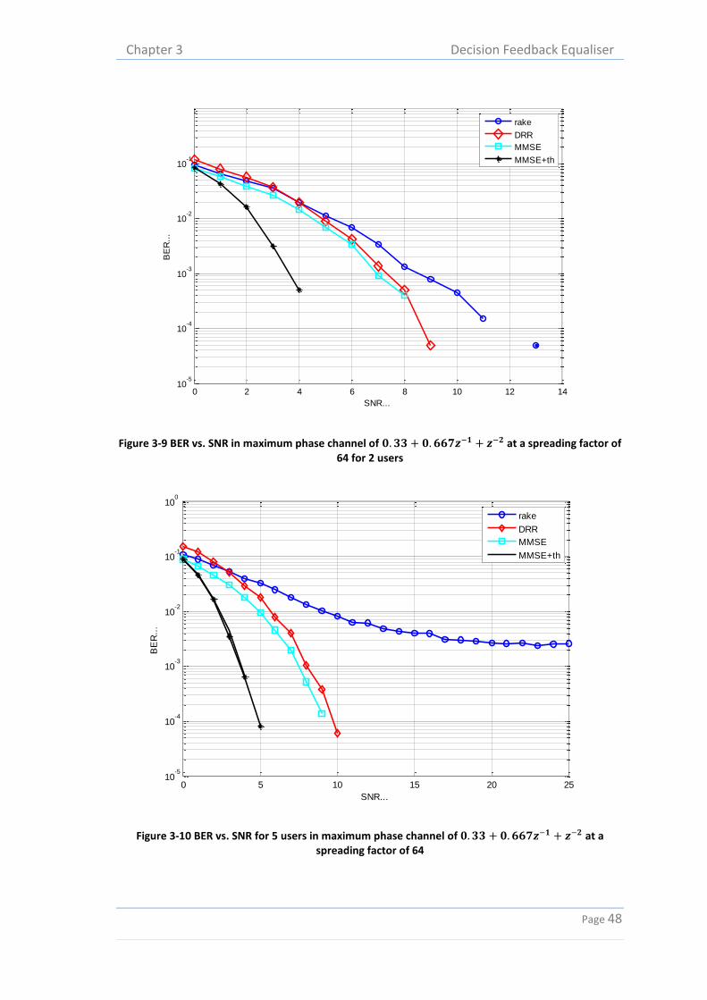
Figure 3-9 BER vs. SNR in maximum phase channel of at a

spreading factor of 64 for 2 users ............................................................................................ 48

List of Figures

Page vi

Figure 3-10 BER vs. SNR for 5 users in maximum phase channel of

at a spreading factor of 64 ............................................................................................. 48

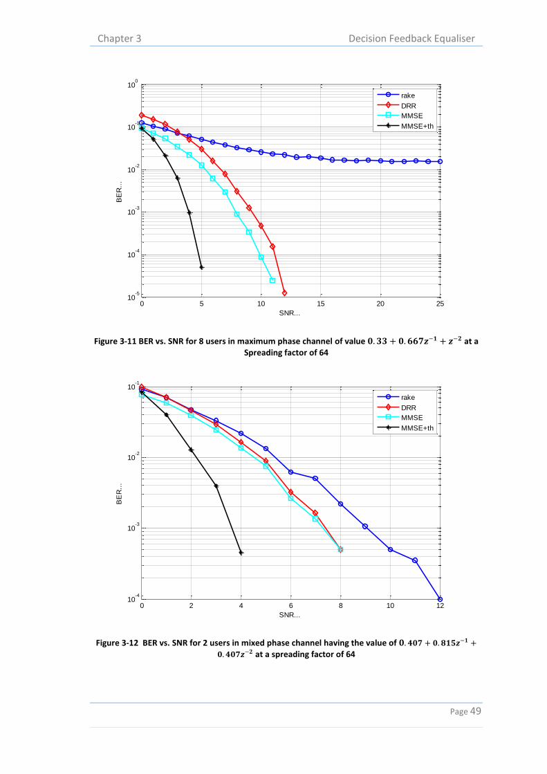
Figure 3-11 BER vs. SNR for 8 users in maximum phase channel of value

at a Spreading factor of 64 ...................................................................................... 49

Figure 3-12 BER vs. SNR for 2 users in mixed phase channel having the value of

at a spreading factor of 64 ......................................................... 49

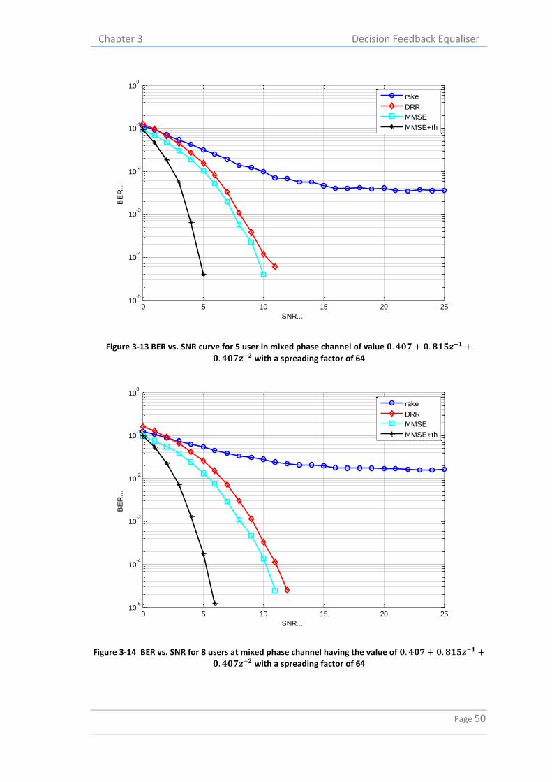
Figure 3-13 BER vs. SNR curve for 5 user in mixed phase channel of value

with a spreading factor of 64 ..................................................... 50

Figure 3-14 BER vs. SNR for 8 users at mixed phase channel having the value of

with a spreading factor of 64 ..................................................... 50

Figure 3-15 BER vs. number of users in minimum phase channel at SNR of 3 dB ................ 51

List of Tables

Page vii

List of Tables Table 2-1 Features of WCDMA .............................................................................................. 10

Nomenclature

Page viii

Nomenclature

* : Convolution

: Knocker Product

: Channel matrix

:

:

:

Covariance matrix

Power of the user

convolution of the transmitted spreading waveform with the

channel impulse response

A : Product between code matrix T and channel matrix H

: Hermitian of matrix A

: Delay of the user

: error symbol

: Spreading factor for user

: Equalised channel weight

: Multi-path fading channel of user

I : Identity Matrix

: Index of the correct symbol at iteration

k : Number of users

p : Cross correlation matrix

R

:

:

Residual matrix

Level of sparity

Nomenclature

Page ix

: Inverse of the autocorrelation matrix

: Minimum distance among symbols of the used constellation

T

:

:

Code Matrix

Symbol duration

: Threshold value at iteration

: column of code matrix T

: Spreading code of user and symbol

w : Additive white Gaussian noise

x : Transmitted symbol

: Estimated front end output

: Estimated symbol using MMSE

: received symbol

: Equalised output signal

Abbreviation

Page x

Abbreviation

1G : First Generation

2G : Second Generation

3G : Third Generation

3GPP : Third Generation Partnership Project

AWGN : Additive White Gaussian Noise

BER : Bit Error Rate

BPSK

CDMA

:

:

Binary Phase Shift Keying

Code Division Multiple Access

CGP : Conjugate Gradient Pursuit

CoSaMP : Compressive Sampling Matching Pursuit

DFE : Decision Feedback Equaliser

DPCH : Dedicated Physical Channels

DPDCH : Dedicated Physical Data Channel

DPDCH : Dedicated Physical Control Channel

EGC

EU

:

:

Equal Gain Combining

Enhanced Uplink

FDD : Frequency Division Duplexing

FDMA : Frequency Division Multiple Access

GP : Gradient Pursuit

HSDPA : High Speed Downlink Packet Access

HSUPA : High Speed Uplink Packet Access

Abbreviation

Page xi

I

IS

:

:

In phase

Interim Standard

ISI : Inter Symbol Interference

LTE : Linear Transversal Equaliser

MAI : Multiple Access Interference

MSE : Mean Square Error

MMSE : Minimum Mean Square Error

MRC : Maximal Ratio Combining

MS : Mobile Station

MUI : Multi User Interference

OMP : Orthogonal Matching Pursuit

OVSF

PDC

Q

:

:

:

Orthogonal Variable Spreading Factor

Personal Digital Cellular

Quadrature phase

QPSK : Quadrature Phase Shift Keying

RR : Rake Receiver

SC-FDMA : Single Carrier Frequency Division Multiple Access

SF : Spreading Factor

SNR : Signal to Noise Ratio

StOMP : Stage-wise Orthogonal Matching Pursuit

TDD : Time Division Duplexing

TDMA : Time Division Multiple Access

TFCI : Transport Format Combination Indicator

UMTS : Universal Mobile Telecommunication Standard

Abbreviation

Page xii

UTRA : UMTS Terrestrial Radio Access

WCDMA : Wideband Code Division Multiple Access

WH : Walsh Hadamard

ZF : Zero Forcing

Abstract

Page xiii

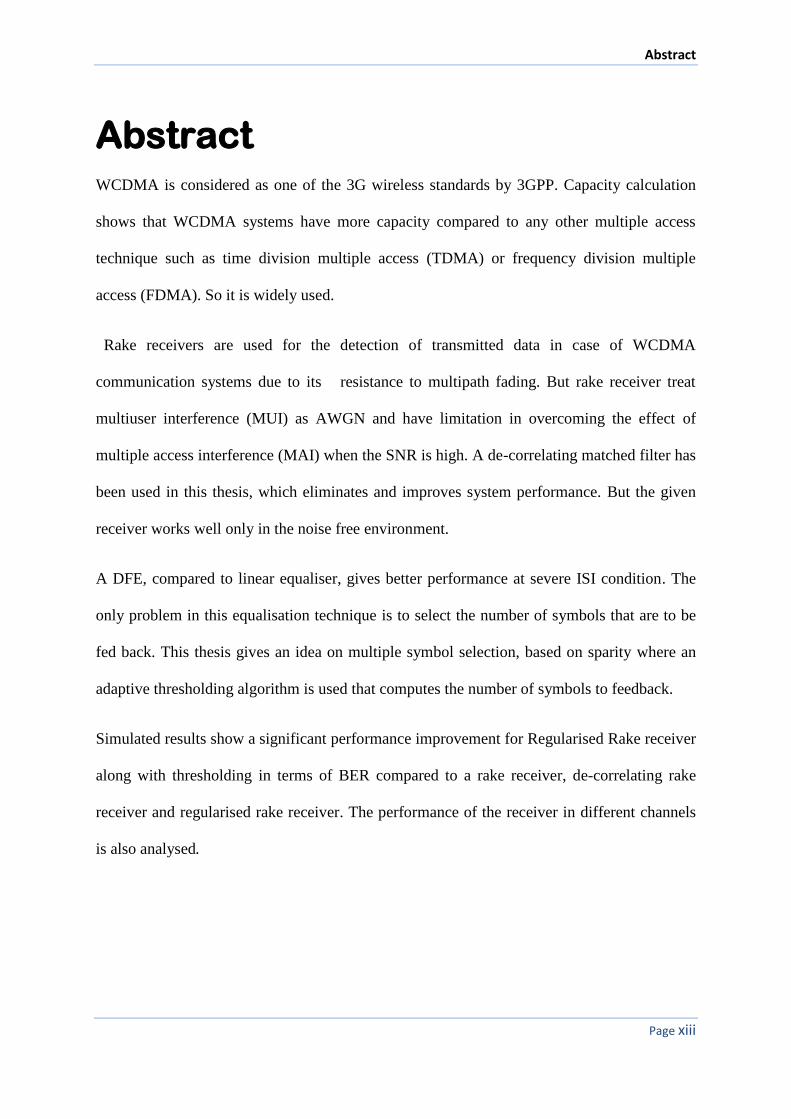
Abstract WCDMA is considered as one of the 3G wireless standards by 3GPP. Capacity calculation

shows that WCDMA systems have more capacity compared to any other multiple access

technique such as time division multiple access (TDMA) or frequency division multiple

access (FDMA). So it is widely used.

Rake receivers are used for the detection of transmitted data in case of WCDMA

communication systems due to its resistance to multipath fading. But rake receiver treat

multiuser interference (MUI) as AWGN and have limitation in overcoming the effect of

multiple access interference (MAI) when the SNR is high. A de-correlating matched filter has

been used in this thesis, which eliminates and improves system performance. But the given

receiver works well only in the noise free environment.

A DFE, compared to linear equaliser, gives better performance at severe ISI condition. The

only problem in this equalisation technique is to select the number of symbols that are to be

fed back. This thesis gives an idea on multiple symbol selection, based on sparity where an

adaptive thresholding algorithm is used that computes the number of symbols to feedback.

Simulated results show a significant performance improvement for Regularised Rake receiver

along with thresholding in terms of BER compared to a rake receiver, de-correlating rake

receiver and regularised rake receiver. The performance of the receiver in different channels

is also analysed.

Chapter 1 Introduction

Page 1

1 Introduction

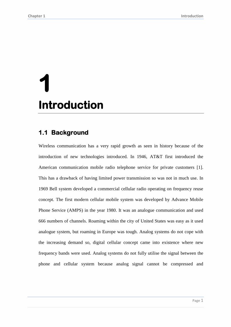
1.1 Background

Wireless communication has a very rapid growth as seen in history because of the

introduction of new technologies introduced. In 1946, AT&T first introduced the

American communication mobile radio telephone service for private customers [1].

This has a drawback of having limited power transmission so was not in much use. In

1969 Bell system developed a commercial cellular radio operating on frequency reuse

concept. The first modern cellular mobile system was developed by Advance Mobile

Phone Service (AMPS) in the year 1980. It was an analogue communication and used

666 numbers of channels. Roaming within the city of United States was easy as it used

analogue system, but roaming in Europe was tough. Analog systems do not cope with

the increasing demand so, digital cellular concept came into existence where new

frequency bands were used. Analog systems do not fully utilise the signal between the

phone and cellular system because analog signal cannot be compressed and

Chapter 1 Introduction

2 | P a g e

manipulated as easily as compared to the digital signal. GSM system was considered as

the first digital cellular system.

1.1.1 Advantages and Disadvantages of Wireless

Communication

Advantages

There are a number of advantages of wireless communication over wired

communication. Some of them include mobility, increased reliability, rapid disaster

recovery, ease of installation and low cost.

Mobility: The primary advantage of wireless communication is the freedom of moving

that it provides to the user while communicating with someone. This means the user is

not bound to be fixed at a place as in wired communication.

Increased reliability: The main problem with wired communication is failure of network

or damage to wire because of environment. Thus the wireless communication not only

eliminates the above said problem but also increases reliability.

Rapid Disaster Recovery: Natural disasters are never predictable and they harm the

wires that are not in case of wireless communication.

Ease of Installation: The time to install a network cable may take some days to week

while using wireless LAN eliminates this trouble.

Cost: The cost required in the cables and other hardware equipment is reduced

compared to wireless system.

Chapter 1 Introduction

3 | P a g e

Disadvantage

As all fields have two sides i.e. a brighter and a darker side, the darker side of wireless

communication include radio signal interference, security problems and health hazards.

Signal Interference: Signals from different other wireless devices can interrupt its

transmission or a wireless device may itself be a source of interference for other

wireless devices.

Security: Here in wireless communication device, it transmits signal over a wide range

and thus security becomes major concern.

Health Hazards: The frequency range in which the wireless communication operates is

very high that may cause damage to the sensitive organs.

1.1.2 Mobile Communication 1G to 3G

First Generation Analog Cellular System

The first generation cellular system comprises of analog transmission technology.

Mostly AMPS was developed in this generation in most parts of US, South America,

Australia and China. It uses frequency modulation (FM) for transmitting the signal.

Here the entire service area is divided into number of cells and each cell is allocated

with a unique frequency band. For frequency reuse concept the frequency band is

divided among seven cells that improves the voice quality as each subscriber uses larger

bandwidth. It uses a channel bandwidth of 30 KHz in 800MHz spectrum. This system

uses two separate bands for uplink and downlink.

Second Generation Digital Cellular System

The second generation deals with digital transmission technology. The digital cellular

technology compared to analog system supports larger subscribers within the given

Chapter 1 Introduction

4 | P a g e

frequency band thus supports higher user capacity, superior voice quality as well as

security. To have efficient use of frequency spectrum, it uses time division and code

division multiple access technique that transmits low data rate as well as voice. A 2G

system mainly comprises of four standards i.e. North American Interim Standard (IS-

54), GSM, the pan-European digital cellular; Personal Digital Cellular (PDC) and IS-95

in North America. Among the four, first three use TDMA technique and last one uses

CDMA. As in 1G, 2G system also uses FDD technique i.e. different bands for forward

and reverse link and use the frequency band that ranges 800 MHz - 900 MHz. Here the

signals are transmitted in the form of packets or frames. The length of the packets

should not be short enough, so that the channels do not change significantly during

transmission. The length of packet should not be long enough so that the time interval

between packets should not be smaller than the length of the packet. GSM supports

eight users in 200 KHz band and IS-54 uses three users in 30 KHz band.

Evolution from 2G to 3G

GSM is a digital cellular technology that supports voice as well as data transmission at

a speed of 9.6 kbps along with Short Message Service (SMS). It operates at 800 MHz

and 1.8 GHz band in Europe and 850 MHz and 1.9 GHz band in US. It provides

international roaming and GPRS. Besides GSM the technology also has CDMA

communication standard that supports data as well as multimedia services. It was

started in 1991 as IS-95A. It supports a variable number of users in 1.25 MHz wide

channel. It can operate at high interference environment because of its interference

resistance property.

Chapter 1 Introduction

5 | P a g e

Third Generation

Here the system aims to combine telephony, internet and multimedia to a single device

i.e. it supports high quality images and videos and also supports high data rates.

WCDMA is the most widely used 3G air interfaces. It was developed by Third

Generation Partnership Project (3GPP), which is the joint standardisation project of the

standardisation bodies from Europe, Japan Korea China and USA. WCDMA was

selected as an air interface for Universal Mobile Telecommunication Services (UMTS).

Code Division Multiple Access communication networks have been developed by a

number of companies over the years, but development of cell-phone networks based on

CDMA (prior to W-CDMA) was dominated by Qualcomm [1]. Qualcomm was the first

company to develop a practical and cost-effective CDMA implementation for consumer

cell phones. Its air interface standard IS-95 has since evolved into the current WCDMA

and CDMA2000 standard [2].

1.2 Literature Survey

CDMA was first commercially used in the mid of nineties. After the tremendous

success of IS-95, WCDMA was adopted as the3GPP air interface with initial released in

99 and 4 [2]. Since then WCDMA was used as wireless internet, video telephony

and voice over IP. High speed downlink packet access (HSDPA) is used for packet

switch connectivity in downlink direction as in release 5 in 2002. High speed uplink

packet Access (HSUPA) also known as enhanced uplink (EU) is used to support the

packet in uplink in release 6 in 2004. The HSPA for WCDMA was standardised in

3GPP release 7 known as HSPA+ in June 2007 [2]. A rake receiver that is used in the

receiver section was used to overcome the multiple access interference. It was first

proposed by Prince and Green and patent in 1958 [3]. The main problem with rake

Chapter 1 Introduction

6 | P a g e

receiver is that it treats multiuser interference (MUI) as Additive white Gaussian noise

(AWGN) and is unable to overcome the effect of multiple access interference (MAI).

So, blind two dimensional rake receivers was first proposed by Zoltowski et al in his

paper [4] and further developed in his further papers [5, 6]. In his paper he used the

conventional matched filter in the first stage followed by post processing to mitigate the

effect of multiuser interference. There he used channel estimation via matrix pencil

technique base on second order statistic. De-correlating rake receiver was proposed by

Lang Tong et al [7]. Here he used the rake concept where de-correlating matched filter

was used in the front end to separate users and perform single-user optimal rake

combining as the second step. Here least square estimation was used which has an

advantage of requiring small number of samples. Here the channel estimation as well

symbol detection was proposed that not only gives better performance but also reduces

the computational complexity. The technique works well but at high interference

condition its performance degrades. For that one should go for non-linear equaliser. In

the paper [8, 9] DFE was used to overcome the effect of interference in case of Single

Carrier Frequency Division Multiple Access (SC-FDMA). The paper gives an adaptive

thresholding technique that computes the sparsity solutions and thus decides the number

of symbols used to be fed back.

1.3 Motivation

In case of spread spectrum communication, rake receivers (RR) are used in the receiver

section for the detection of the transmitted symbols. As in case of WCDMA, unique

orthogonal codes are used for each user and the same code is used in the receiver

section to get back the transmitted symbol. The RR works on the principle of multipath

diversity and decodes the received signal. When the signal is transmitted through the

Chapter 1 Introduction

7 | P a g e

channel, then it suffers from multipath propagation and the orthogonality of the code is

lost. As the code orthogonality is lost RR is unable to work properly. So we go for

different equalisation technique to overcome the above effect.

Equalisation technique is used to overcome the effect of inter symbol interference [10].

Linear equalisation is preferred as they are simple and easy to build. But at severe ISI

condition they are unable to work properly so a non-linear equaliser is preferred at high

interference environment. A DFE non-linear equaliser is used that lowers the

interference level and improves the performance in terms of BER. The DFE comprises

of a feed forward and a feedback path along with a decision device. An adaptive

thresholding is used in the decision devise of DFE that helps in improving the

performance.

1.4 Thesis Outline

This thesis is organised into four chapters. The first chapter deals with the introduction

to wireless and mobile communication and different technology used in different

generations. The chapter ends with the outline of the thesis.

The second chapter deals with the basics related to WCDMA. There the multipath

propagation and the receiver that is used are given in details. Here a notation is used to

describe the received signal. The working of rake receiver is briefly explained in this

chapter.

Next chapter starts with a brief introduction to different equalisation technique. It was

found that non-linear equalisation technique gives better performance so they are

discussed briefly in this part. The simulation results are also shown in this chapter that

give a comparative study between different equalisation techniques.

Chapter 1 Introduction

8 | P a g e

The last chapter is the summary and the discussion on the work presented in this thesis.

It deals with the limitations and also outlines the future work.

Chapter 2 WCDMA

Page 9

2

WCDMA

2.1 Introduction

Wideband Code Division Multiple Access (WCDMA) also known as UMTS Terrestrial

radio Access (UTRA). It was first developed by Third Generation Partnership Project

(3GPP) [2] which is the joint standardisation project of the standardisation bodies from

Europe, Japan, Korea, the USA and China. It has a band width of about 5MHz. Because

of this large bandwidth it’s named as Wideband CDMA or Wideband Code Division

Multiple Access. Here we can use two modes for communication i.e. Frequency

Division Duplexing (FDD) and Time Division Duplexing (TDD).

In TDD mode, uplink and downlink transmission is performed in the same frequency

band but they are differentiated by allotting separate time slots. It is a transmission

scheme that allows asymmetric flow for uplink and downlink data transmission. Here

users are allocated time slots for uplink and downlink transmission.

Chapter 2 WCDMA

Page 10

In FDD two separate frequency bands are allotted for the uplink and downlink

transmission. A pair of frequency bands with specified separation is assigned for a

connection.

Uplink is the connection from mobile to base station and downlink is the reverse one

i.e. connection from base station to mobile.

2.1.1 Specification

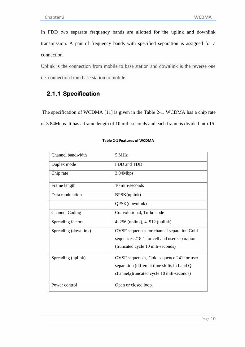
The specification of WCDMA [11] is given in the Table 2-1. WCDMA has a chip rate

of 3.84Mcps. It has a frame length of 10 mili-seconds and each frame is divided into 15

Table 2-1 Features of WCDMA

Channel bandwidth 5 MHz

Duplex mode FDD and TDD

Chip rate 3.84Mbps

Frame length 10 mili-seconds

Data modulation BPSK(uplink)

QPSK(downlink)

Channel Coding Convolutional, Turbo code

Spreading factors 4–256 (uplink), 4–512 (uplink)

Spreading (downlink) OVSF sequences for channel separation Gold

sequences 218-1 for cell and user separation

(truncated cycle 10 mili-seconds)

Spreading (uplink) OVSF sequences, Gold sequence 241 for user

separation (different time shifts in I and Q

channel,(truncated cycle 10 mili-seconds)

Power control Open or closed loop.

Chapter 2 WCDMA

Page 11

slots. Here the spreading factor can be different for uplink and downlink. The ratio of

the chip rate to the data rate is called the spreading factor. The spreading factor for

uplink ranges from 256 to 4 while for downlink it is 512 to 4.

2.1.2 Features of WCDMA

Some of the features of the WCDMA are given as below:

It supports high data rate transmission i.e. 384 Kbps with wide area coverage

and 2 Mbps of local coverage.

It has high service flexibility i.e. it supports multiple parallel variable rate

services on each connection.

It operates on both Frequency Division Duplex (FDD) and Time Division

Duplex (TDD)

It has an ability to support for future capacity and coverage enhancing

technologies like adaptive antennas, advanced receiver structures and

transmitter diversity.

It supports inter-frequency hand over and the hand over among other systems,

including handover to GSM.

Has efficient packet access capability.

It employs coherent detection on uplink and downlink based on the use of pilot

symbols.

One of the important features of WCDMA is soft handover, which is supported

by simultaneously delivering data to mobile from different base station.

It provides multipath diversity for small cells.

Chapter 2 WCDMA

Page 12

Advantage of WCDMA

Some of the advantages of WCDMA include:

Service flexibility-WCDMA has a capability to allow carrier of 5MHz to

process mixed service from 8Kbps to 2Mbps. In also supports circuit switched

service and packet switched service in the same channel, and a single terminal is

used for carrying out multiple circuits and packets switched services, and thus

realize genuine multimedia service. It supports services with different

requirements such as voice and packet data and also ensures high quality and

perfect coverage.

Spectrum efficiency- WCDMA has the ability of making the efficient use of

available radio spectrums. Here no frequency planning is required as a single

cell multiplexing is adopted. Network capacity can be improved drastically by

using technologies of hierarchical cell structure, coherent de-modulation and

adaptive antenna array.

Capacity and Coverage- This has an increased number of voice users which is

about eight times when compared with a typical narrowband transceiver. Here at

a time, the RF carriers can handle about 80 voice calling users or about fifty

internet data users.

Every connection can provide multiple services: Circuit and packet switched

services can be mixed freely in different band width and can be provided to the

same user in the same time instance. Every WCDMA terminal can access up to

six different types of services, which can be the combination of various data

services such as video, e-mails, voice, fax, etc.

Chapter 2 WCDMA

Page 13

Network scale economics – If a digital cellular network, such as GSM, is

working in two systems and WCDMA wireless access is added to it then also

the same multiplexed core network and the same base stations can be used. The

latest ATM mode i.e. micro-cell transmission procedure is used for the links

between WCDMA access network and GSM core network. Using this method

high data packets can be processed effectively, which can further enhance the

capacity of standard E1/T1 lines to 300 voice calls compared to 30 voice calls

for that of existing network. It is found that about 50% transmission cost has

been saved using this multiple access technique.

Outstanding voice capability - Although the main purpose for the next

generation mobile access is to transmit high bit rate data, along with the voice

communication, it can also support other specs.

2.2 Spreading Codes

The codes that are used for spreading the transmitted sequence can be long codes or

short codes. Some of the well-known codes are Walsh-Hadamard codes (WH codes),

m-sequences, Gold codes and Kasami codes. Walsh codes are orthogonal on zero code

delay whereas the m-sequences, Gold codes and Kasami codes are non-orthogonal

codes with varying cross-correlation properties. Gold codes and Walsh-Hadamard

codes are used in uplink communication of WCDMA. The signals are spread using the

orthogonal variable spreading factor (OVSF) codes and are then scrambled using the p-

n codes that helps in differentiating different base stations. Scrambling is done on top of

spreading which is shown in Figure 2-1

Chapter 2 WCDMA

Page 14

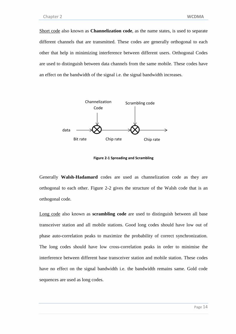
Short code also known as Channelization code, as the name states, is used to separate

different channels that are transmitted. These codes are generally orthogonal to each

other that help in minimizing interference between different users. Orthogonal Codes

are used to distinguish between data channels from the same mobile. These codes have

an effect on the bandwidth of the signal i.e. the signal bandwidth increases.

Figure 2-1 Spreading and Scrambling

Generally Walsh-Hadamard codes are used as channelization code as they are

orthogonal to each other. Figure 2-2 gives the structure of the Walsh code that is an

orthogonal code.

Long code also known as scrambling code are used to distinguish between all base

transceiver station and all mobile stations. Good long codes should have low out of

phase auto-correlation peaks to maximize the probability of correct synchronization.

The long codes should have low cross-correlation peaks in order to minimise the

interference between different base transceiver station and mobile station. These codes

have no effect on the signal bandwidth i.e. the bandwidth remains same. Gold code

sequences are used as long codes.

data

Channelization

Code Scrambling code

Bit rate Chip rate Chip rate

Chapter 2 WCDMA

Page 15

2.2.1 Walsh-Hadamard code

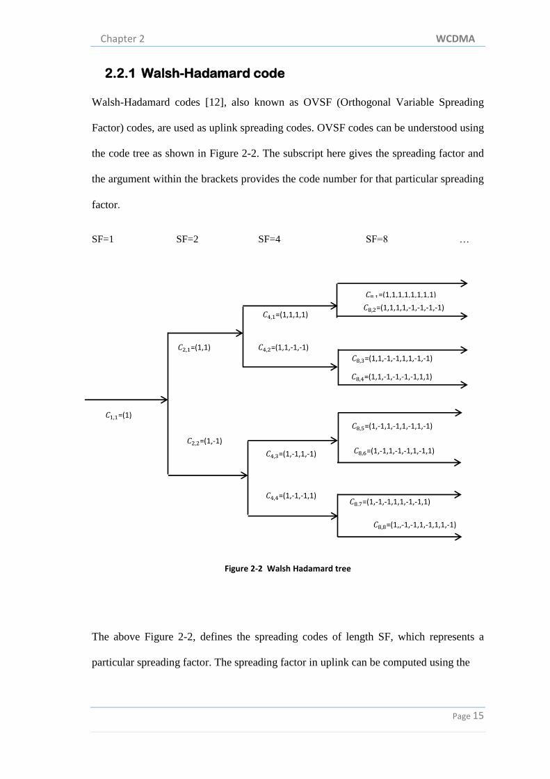
Walsh-Hadamard codes [12], also known as OVSF (Orthogonal Variable Spreading

Factor) codes, are used as uplink spreading codes. OVSF codes can be understood using

the code tree as shown in Figure 2-2. The subscript here gives the spreading factor and

the argument within the brackets provides the code number for that particular spreading

factor.

SF=1 SF=2 SF=4 SF=8 …

Figure 2-2 Walsh Hadamard tree

The above Figure 2-2, defines the spreading codes of length SF, which represents a

particular spreading factor. The spreading factor in uplink can be computed using the

=(1,1,1,1,1,1,1,1)

=(1,,-1,-1,1,-1,1,1,-1)

𝐶 2=(1,1,1,1,-1,-1,-1,-1)

𝐶 3=(1,1,-1,-1,1,1,-1,-1)

𝐶 4=(1,1,-1,-1,-1,-1,1,1)

𝐶 5=(1,-1,1,-1,1,-1,1,-1)

𝐶 6=(1,-1,1,-1,-1,1,-1,1)

𝐶 7=(1,-1,-1,1,1,-1,-1,1)

𝐶4 =(1,1,1,1)

𝐶4 2=(1,1,-1,-1)

𝐶4 3=(1,-1,1,-1)

𝐶4 4=(1,-1,-1,1)

𝐶2 =(1,1)

𝐶2 2=(1,-1)

𝐶 =(1)

Chapter 2 WCDMA

Page 16

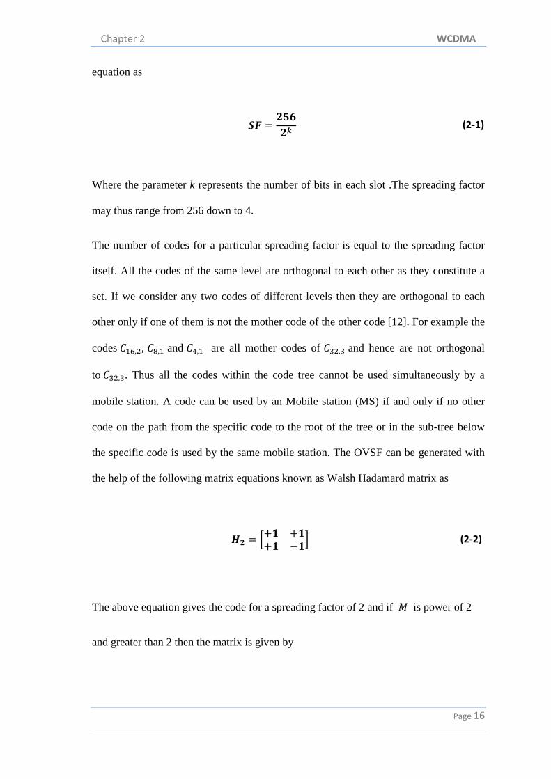
equation as

(2-1)

Where the parameter k represents the number of bits in each slot .The spreading factor

may thus range from 256 down to 4.

The number of codes for a particular spreading factor is equal to the spreading factor

itself. All the codes of the same level are orthogonal to each other as they constitute a

set. If we consider any two codes of different levels then they are orthogonal to each

other only if one of them is not the mother code of the other code [12]. For example the

codes 6 2, and 4 are all mother codes of 32 3 and hence are not orthogonal

to 32 3. Thus all the codes within the code tree cannot be used simultaneously by a

mobile station. A code can be used by an Mobile station (MS) if and only if no other

code on the path from the specific code to the root of the tree or in the sub-tree below

the specific code is used by the same mobile station. The OVSF can be generated with

the help of the following matrix equations known as Walsh Hadamard matrix as

[

] (2-2)

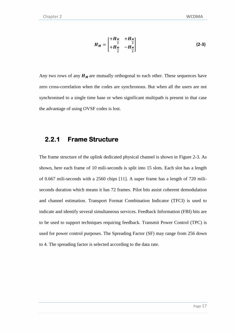
The above equation gives the code for a spreading factor of 2 and if is power of 2

and greater than 2 then the matrix is given by

Chapter 2 WCDMA

Page 17

[

] (2-3)

Any two rows of any are mutually orthogonal to each other. These sequences have

zero cross-correlation when the codes are synchronous. But when all the users are not

synchronised to a single time base or when significant multipath is present in that case

the advantage of using OVSF codes is lost.

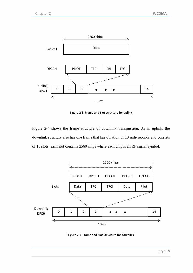
2.2.1 Frame Structure

The frame structure of the uplink dedicated physical channel is shown in Figure 2-3. As

shown, here each frame of 10 mili-seconds is split into 15 slots. Each slot has a length

of 0.667 mili-seconds with a 2560 chips [11]. A super frame has a length of 720 mili-

seconds duration which means it has 72 frames. Pilot bits assist coherent demodulation

and channel estimation. Transport Format Combination Indicator (TFCI) is used to

indicate and identify several simultaneous services. Feedback Information (FBI) bits are

to be used to support techniques requiring feedback. Transmit Power Control (TPC) is

used for power control purposes. The Spreading Factor (SF) may range from 256 down

to 4. The spreading factor is selected according to the data rate.

Chapter 2 WCDMA

Page 18

Figure 2-3 Frame and Slot structure for uplink

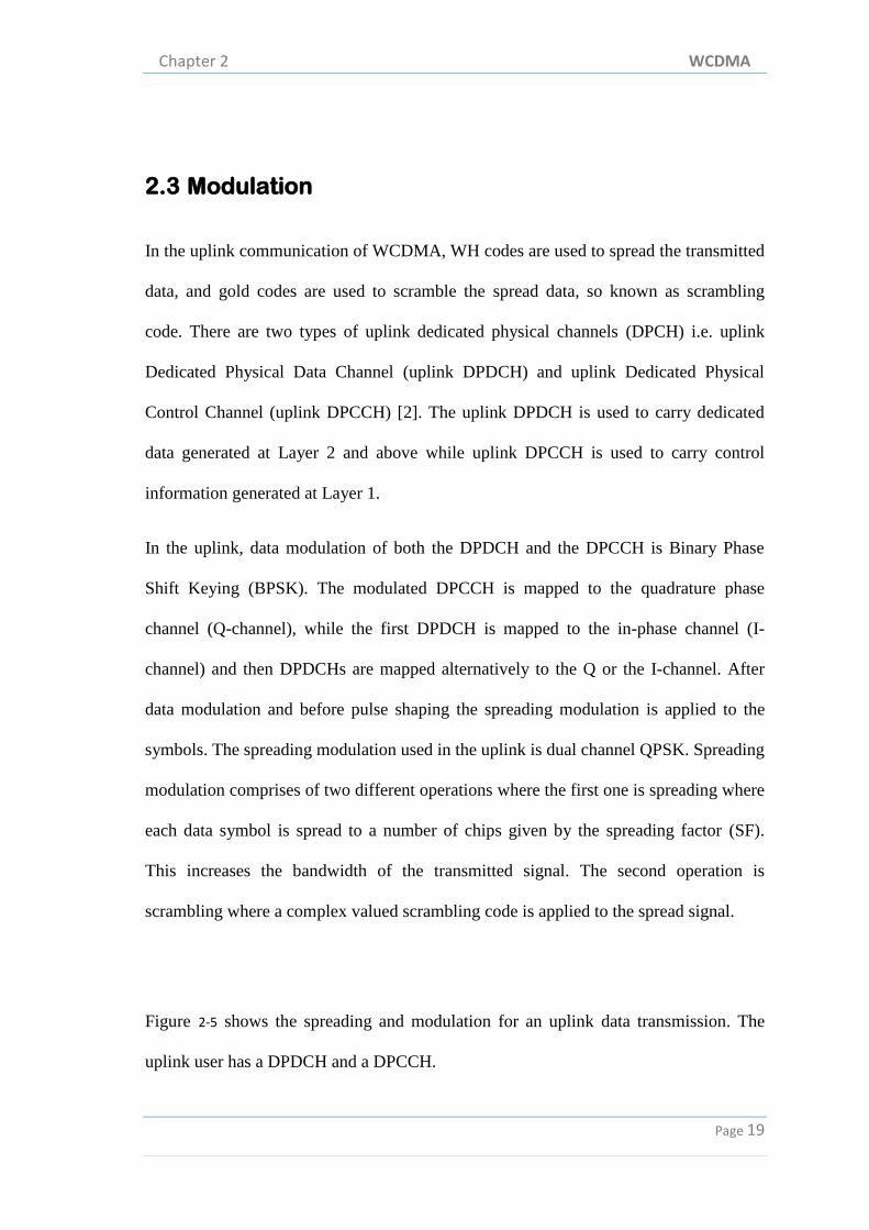
Figure 2-4 shows the frame structure of downlink transmission. As in uplink, the

downlink structure also has one frame that has duration of 10 mili-seconds and consists

of 15 slots; each slot contains 2560 chips where each chip is an RF signal symbol.

Figure 2-4 Frame and Slot Structure for downlink

0 1 3 14

PILOT TFCI FBI TPC

Data

2560 chips

DPDCH

DPCCH

Uplink

DPCH

10 ms

0 1 2 3 14 Downlink

DPCH

Data TPC TFCI Data Pilot

DPDCH DPCCH DPCCH DPCCH DPDCH

10 ms

2560 chips

Slots

Chapter 2 WCDMA

Page 19

2.3 Modulation

In the uplink communication of WCDMA, WH codes are used to spread the transmitted

data, and gold codes are used to scramble the spread data, so known as scrambling

code. There are two types of uplink dedicated physical channels (DPCH) i.e. uplink

Dedicated Physical Data Channel (uplink DPDCH) and uplink Dedicated Physical

Control Channel (uplink DPCCH) [2]. The uplink DPDCH is used to carry dedicated

data generated at Layer 2 and above while uplink DPCCH is used to carry control

information generated at Layer 1.

In the uplink, data modulation of both the DPDCH and the DPCCH is Binary Phase

Shift Keying (BPSK). The modulated DPCCH is mapped to the quadrature phase

channel (Q-channel), while the first DPDCH is mapped to the in-phase channel (I-

channel) and then DPDCHs are mapped alternatively to the Q or the I-channel. After

data modulation and before pulse shaping the spreading modulation is applied to the

symbols. The spreading modulation used in the uplink is dual channel QPSK. Spreading

modulation comprises of two different operations where the first one is spreading where

each data symbol is spread to a number of chips given by the spreading factor (SF).

This increases the bandwidth of the transmitted signal. The second operation is

scrambling where a complex valued scrambling code is applied to the spread signal.

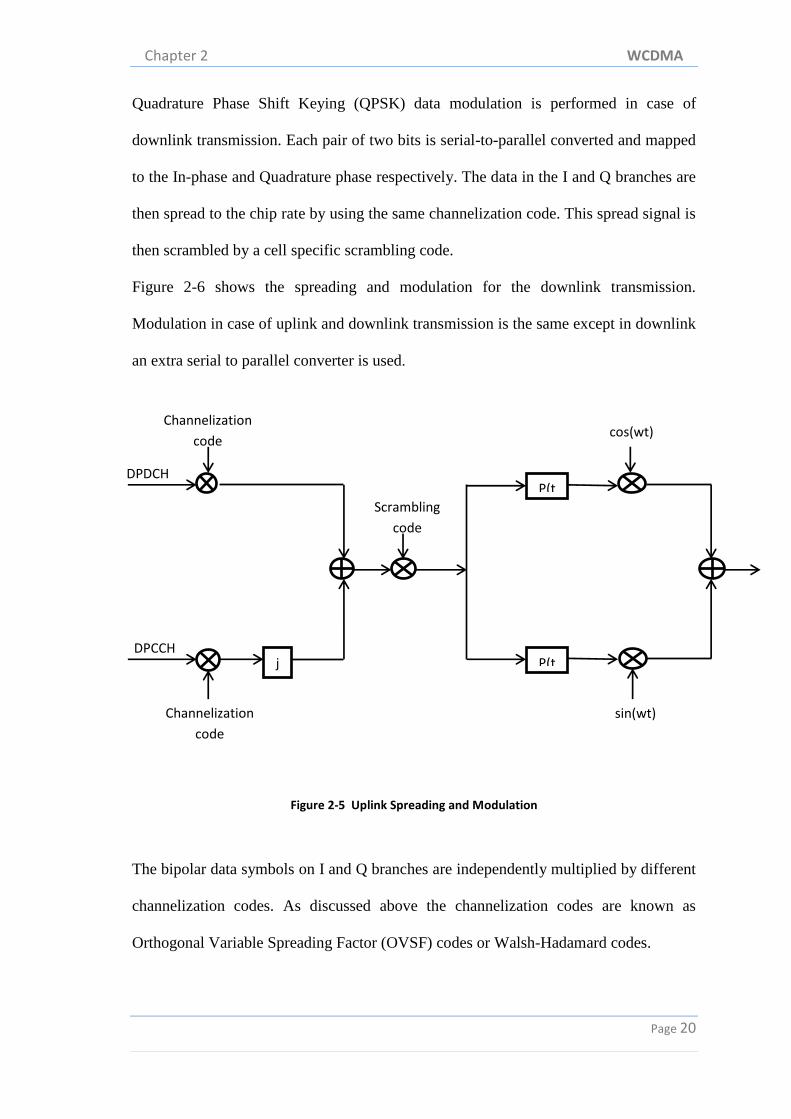
Figure 2-5 shows the spreading and modulation for an uplink data transmission. The

uplink user has a DPDCH and a DPCCH.

Chapter 2 WCDMA

Page 20

Quadrature Phase Shift Keying (QPSK) data modulation is performed in case of

downlink transmission. Each pair of two bits is serial-to-parallel converted and mapped

to the In-phase and Quadrature phase respectively. The data in the I and Q branches are

then spread to the chip rate by using the same channelization code. This spread signal is

then scrambled by a cell specific scrambling code.

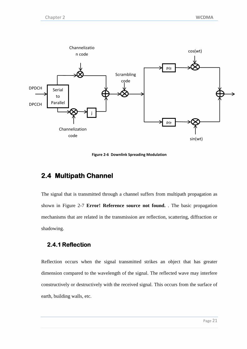
Figure 2-6 shows the spreading and modulation for the downlink transmission.

Modulation in case of uplink and downlink transmission is the same except in downlink

an extra serial to parallel converter is used.

Figure 2-5 Uplink Spreading and Modulation

The bipolar data symbols on I and Q branches are independently multiplied by different

channelization codes. As discussed above the channelization codes are known as

Orthogonal Variable Spreading Factor (OVSF) codes or Walsh-Hadamard codes.

DPDCH

Channelization

code

DPCCH

Channelization

code

j

Scrambling

code

P(t

P(t

cos(wt)

sin(wt)

Chapter 2 WCDMA

Page 21

Figure 2-6 Downlink Spreading Modulation

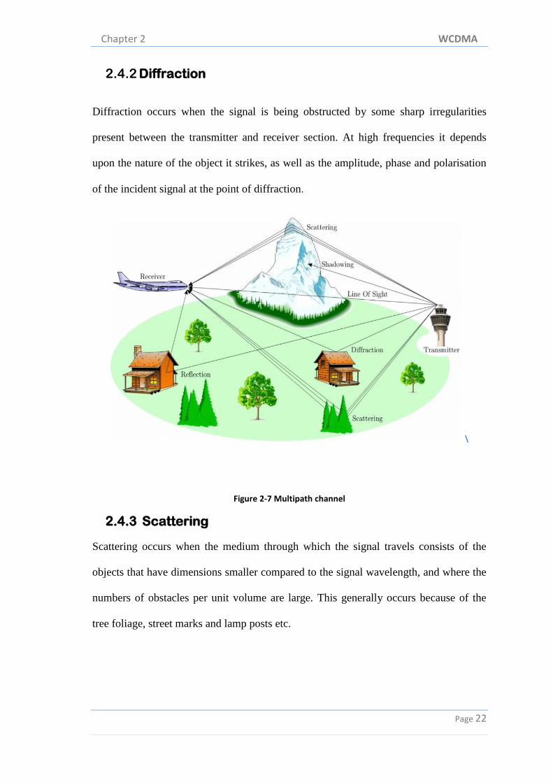
2.4 Multipath Channel

The signal that is transmitted through a channel suffers from multipath propagation as

shown in Figure 2-7 Error! Reference source not found. . The basic propagation

mechanisms that are related in the transmission are reflection, scattering, diffraction or

shadowing.

2.4.1 Reflection

Reflection occurs when the signal transmitted strikes an object that has greater

dimension compared to the wavelength of the signal. The reflected wave may interfere

constructively or destructively with the received signal. This occurs from the surface of

earth, building walls, etc.

DPDCH

Channelizatio

n code

DPCCH

Channelization

code

j

Scrambling

code

P(t

P(t

cos(wt)

sin(wt)

Serial

to

Parallel

Chapter 2 WCDMA

Page 22

2.4.2 Diffraction

Diffraction occurs when the signal is being obstructed by some sharp irregularities

present between the transmitter and receiver section. At high frequencies it depends

upon the nature of the object it strikes, as well as the amplitude, phase and polarisation

of the incident signal at the point of diffraction.

\

Figure 2-7 Multipath channel

2.4.3 Scattering

Scattering occurs when the medium through which the signal travels consists of the

objects that have dimensions smaller compared to the signal wavelength, and where the

numbers of obstacles per unit volume are large. This generally occurs because of the

tree foliage, street marks and lamp posts etc.

Chapter 2 WCDMA

Page 23

2.4.4 Shadowing

Shadowing occurs when large object block the path of propagation of the signal. Here

the signal is unable to propagate and thus it is transmitted from the transmitter section

but never reaches the destination i.e. the receiver section.

2.5 Rake Receiver

The conventional Rake receiver was first given by R Price and P E Green and patent in

the year 1958 [10, 13]. Sometimes it’s also known as diversity combiner. As the name

states, it has the similar feature with that of the garden rake. A rake receiver is used that

counters the effect of multipath fading. Rake receiver does this by using several sub-

receivers, also known as fingers, each delayed slightly in order to tune with the delayed

multipath component. Each component is decoded but at the later stage combined

coherently in order to make use of the different transmission characteristic of each

transmission path.

2.5.1 Different Combining Techniques

Different combining techniques that are used in the reception side are

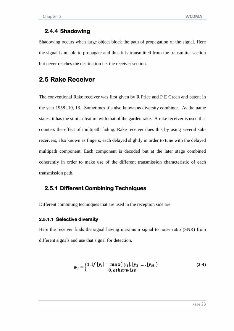
2.5.1.1 Selective diversity

Here the receiver finds the signal having maximum signal to noise ratio (SNR) from

different signals and use that signal for detection.

{ | | {| | | | | |}

(2-4)

Chapter 2 WCDMA

Page 24

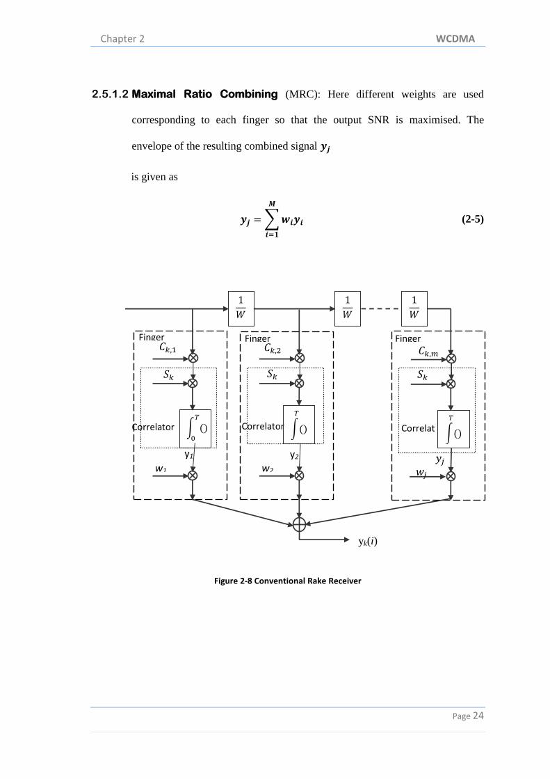
2.5.1.2 Maximal Ratio Combining (MRC): Here different weights are used

corresponding to each finger so that the output SNR is maximised. The

envelope of the resulting combined signal

is given as

∑

(2-5)

Figure 2-8 Conventional Rake Receiver

𝑆𝑘 𝑆𝑘 𝑆𝑘

𝐶𝑘 𝑚 𝐶𝑘 𝐶𝑘 2

1

𝑊

1

𝑊

1

𝑊

Correlator 𝑇

0

w1

Finger

Correlator

or

𝑇

0

w2

Finger

Correlat

or

𝑇

0

𝑤𝑗

Finger

yk(i)

y1 y2 𝑦𝑗

Chapter 2 WCDMA

Page 25

2.5.1.3 Equal Gain Combining (EGC): Here this method maximises the SNR of

the received combined signal. The main drawback of maximal gain combining

is that the receiver complexity increases. So, this combining method is used

that reduces complexity as all the weights are same i.e.

(2-6)

The weight is considered to be ‘one’ and output signal is given by

∑

(2-7)

Out of three, maximal ratio combining is generally used because of its advantage of

producing output with an acceptable SNR even when none of the signals are acceptable.

This combining technique gives the best reduction in fading compared to other

techniques so is mostly used.

A rake receiver collects the signal energy of different multipath components [13]. The

optimal RAKE receiver actually implements a channel matched filer which maximizes

the received signal to noise ratio. This means that the identified multipath components

are weighted proportionally to the amplitude of the component. A typical rake receiver

for WCDMA can contain 3 to 6 number of fingers.

Chapter 2 WCDMA

Page 26

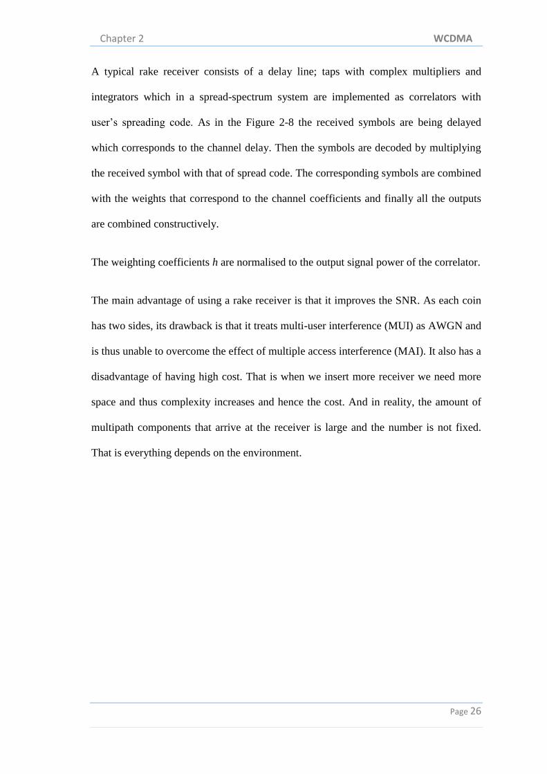
A typical rake receiver consists of a delay line; taps with complex multipliers and

integrators which in a spread-spectrum system are implemented as correlators with

user’s spreading code. As in the Figure 2-8 the received symbols are being delayed

which corresponds to the channel delay. Then the symbols are decoded by multiplying

the received symbol with that of spread code. The corresponding symbols are combined

with the weights that correspond to the channel coefficients and finally all the outputs

are combined constructively.

The weighting coefficients h are normalised to the output signal power of the correlator.

The main advantage of using a rake receiver is that it improves the SNR. As each coin

has two sides, its drawback is that it treats multi-user interference (MUI) as AWGN and

is thus unable to overcome the effect of multiple access interference (MAI). It also has a

disadvantage of having high cost. That is when we insert more receiver we need more

space and thus complexity increases and hence the cost. And in reality, the amount of

multipath components that arrive at the receiver is large and the number is not fixed.

That is everything depends on the environment.

Chapter 3 Decision Feedback Equaliser

Page 27

3 Decision Feedback Equaliser

A wireless channel is generally dispersive i.e. after the signal being transmitted; a

system will receive multiple copies of the signal, with different channel gain, at

different instance of time. This dispersion in time, in the channel causes inter-symbol

interference (ISI) and thus the performance of the system degrades. Thus to overcome

the effect of ISI, a number of equalisation techniques are used. The channel equaliser

can be broadly classified as linear equaliser and non-linear equaliser. A linear equaliser

like a zero forcing equaliser (ZFE) forces the ISI to reduce to zero when the channel is

noiseless. But when the channel is noisy, it enhances the noise. This causes degradation

of the performance, hence rarely used. Another type of equaliser i.e. minimum mean

square equaliser (MMSE) is used that performs better than the ZFE as it takes noise into

account. But its performance is not enough for channels with severe ISI. So a non-linear

equaliser i.e. a decision feedback equaliser is used.

A DFE is a non-linear equaliser that uses previous detected decisions to eliminate ISI

on the current received symbol. The basic idea behind the DFE is to subtract from our

Chapter 3 Decision Feedback Equaliser

Page 28

observation at the receiver (feed back to the receiver) correctly detected symbols in

order to reduce the interference for the currently equalized symbols. A standard DFE

has two filters i.e. feed forward filter and feedback filter.

3.1 Introduction

Equalisers are used to mitigate the effect of ISI [14]. The main advantage of this

approach is that a digital filter is easy to build and is easy to alter for different

equalization schemes, and also to fit different channel conditions. So equaliser can be

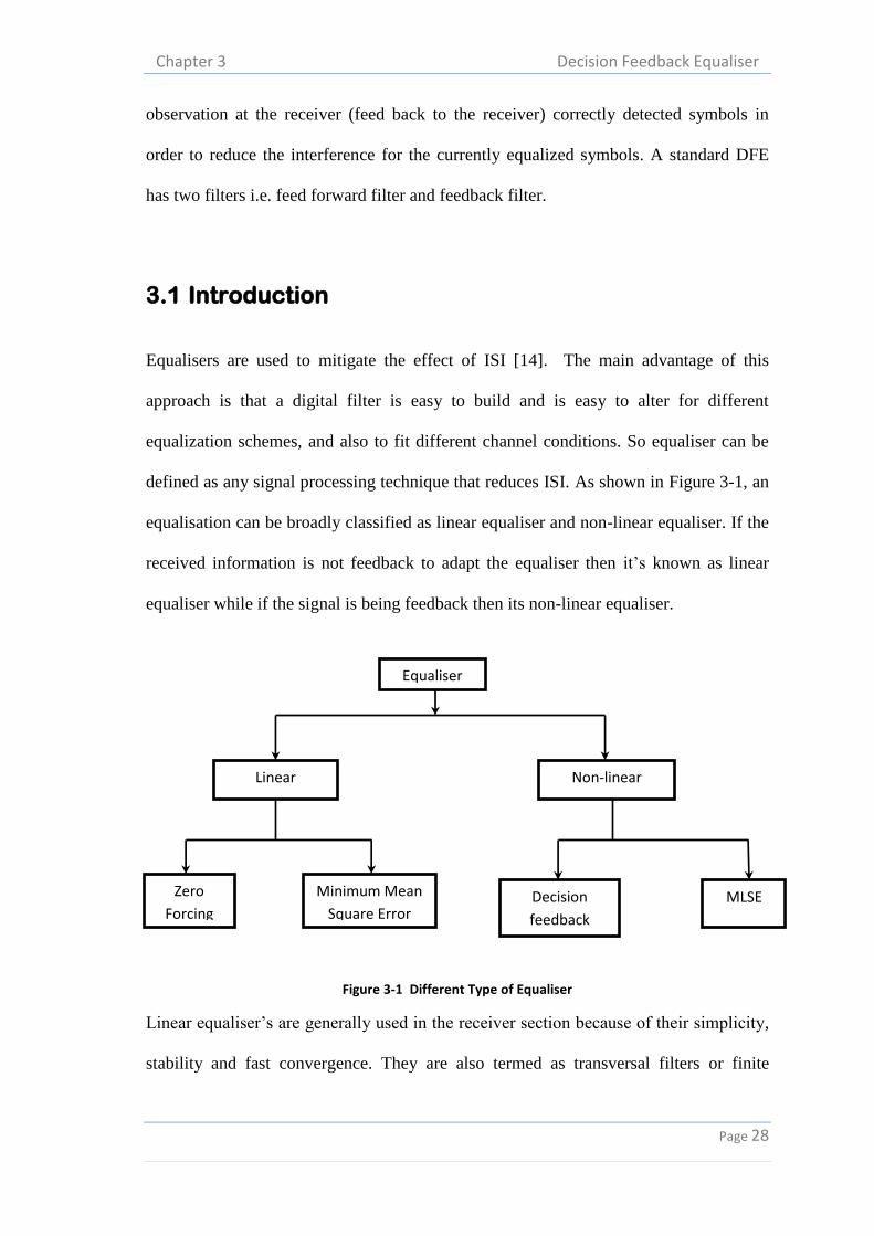
defined as any signal processing technique that reduces ISI. As shown in Figure 3-1, an

equalisation can be broadly classified as linear equaliser and non-linear equaliser. If the

received information is not feedback to adapt the equaliser then it’s known as linear

equaliser while if the signal is being feedback then its non-linear equaliser.

Figure 3-1 Different Type of Equaliser

Linear equaliser’s are generally used in the receiver section because of their simplicity,

stability and fast convergence. They are also termed as transversal filters or finite

Equaliser

Linear Non-linear

Zero

Forcing

Minimum Mean

Square Error Decision

feedback

MLSE

Chapter 3 Decision Feedback Equaliser

Page 29

impulse response (FIR) filter. Some of the linear equaliser that is commonly used is

Zero Forcing equaliser (ZF) and Minimum Mean Square Error equaliser (MMSE).

3.1.1 Zero Forcing

One of the simplest ways to remove ISI is by choosing the transfer function of the

equaliser such that the output of equaliser gives back the transmitted information, only

if noise is not present, which mean ZF equaliser applies the inverse of the channel

frequency response to the conventional detected output in order to restore the received

information from the channel

.

This technique is called zero forcing equalisation because ISI component at the

equaliser output is forced to zero. Thus it has an advantage of eliminating multiple

access interference (MAI) and has less computational complexity compared to

maximum likelihood sequence estimator (MLSE). In this type of equalisation, the effect

of noise is neglected, but practically noise exists in environment. Although ISI is forced

to zero, there is a chance to enhance the noise power by the equaliser. Hence the error

performance of the receiver still gets poorer. One more problem of using this technique

is the computation needed to inverse the correlation matrix is difficult to perform in real

time.

3.1.2 Minimum mean Square Error

Although zero forcing equaliser removes ISI, but it may not give best error performance

in communication environment as it does not take noises into account in the system. So

we go for minimum mean square error equalisation (MMSE) [7, 15] which is based on

mean square error criteria. It was patent by Lucky in the year 1965 [10]. A linear

Chapter 3 Decision Feedback Equaliser

Page 30

equalizer is being used that minimizes the mean square error between the received

signal and the output of the equaliser . The mean square error is given as

[ ] [

] (3-1)

To compute minimum mean square error the derivative of the above equation with

respect to is taken and is equated to 0.

Solving the above equation we get

(3-2)

Where

[ ] (3-3)

[ ] (3-4)

If R and p are known, then the MMSE equalizer can be found by solving the linear

matrix Equation (3-2). It can be shown that the signal-to-noise ratio at the output of the

MMSE equalizer is better than that of the zero-forcing equalizer. This type of equaliser

is most popularly known as Linear Transversal Equaliser (LTE).

The linear MMSE equalizer can also be found iteratively. The gradient of the MSE with

respect to h gives the direction to change for the largest increase of the MSE. To

Chapter 3 Decision Feedback Equaliser

Page 31

decrease MSE one can update in the opposite direction to the gradient. This is

known as steepest descent algorithm.

3.1.3 Decision Feedback Equaliser

Although MMSE equalizer gives better performance compared to zero forcing

equaliser, but its performance is not enough for channels having high ISI. For that case

non-linear equaliser such as Decision Feedback Equalisation is used. Austin first

published a report on DFE in the year 1967 and further optimization of DFE received

for minimum mean square error was analysed and accomplished by Monsen in the year

1971 [15].

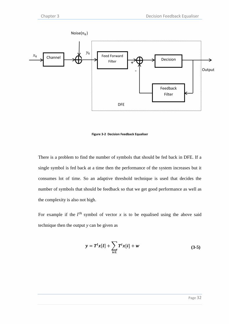
As shown in Figure 3-2 a DFE mainly comprises of a feed forward section and a

feedback section. The feed forward section corresponds to a linear transversal filter

whose taps are spaced by reciprocal of the symbol rate. Similarly feedback filter also

comprises of transversal filter whose taps are spaced by reciprocal of symbol rate. The

input to the feedback filter is fed after the symbol is passed through a decision devise

that operates on the previously detected symbols. The function of feedback section is to

subtract that portion of ISI produced by previously detected symbol from the estimation

of the future detected symbols. Thus DFE reduces the effect of interference. But in the

feedback section if the correct symbols are not fed back then the interference level is

further increased. So it’s very crucial to decide the correct symbols that should be fed so

as to reduce interference.

Chapter 3 Decision Feedback Equaliser

Page 32

Figure 3-2 Decision Feedback Equaliser

There is a problem to find the number of symbols that should be fed back in DFE. If a

single symbol is fed back at a time then the performance of the system increases but it

consumes lot of time. So an adaptive threshold technique is used that decides the

number of symbols that should be feedback so that we get good performance as well as

the complexity is also not high.

For example if the symbol of vector x is to be equalised using the above said

technique then the output y can be given as

[ ] ∑ [ ]

(3-5)

Channel

Noise(𝑛𝑘)

Feed Forward

Filter Decision

Feedback

Filter

𝑥𝑘 𝑦𝑘

DFE

+

- Output

Chapter 3 Decision Feedback Equaliser

Page 33

where is the column of the channel code matrix. First term of the equation is the

symbol that is to be equalised which is scaled by the channel. Second term represents

interference that affects the symbol [ ] and is additive white Gaussian noise. If

some of the symbols [ ] where i ϵ P such that P is subset of L, have been correctly

equalised and detected then using that one can compute the summation part i.e.

∑ [ ] and thus interference part is being subtracted from the detected symbol y

and interference is reduced. Thus the process is continued iteratively and in each step

the system is reduced because in each step the column of the system T is reduced that

corresponds to the index of the correctly equalised symbol. Thus, in each iteration the

code matrix size is reduced and we move nearer towards the correct symbol.

The main problem with the above method is to determine which symbols are correctly

equalised and are to be fed back. While feeding back if a wrong symbol is used instead

of correct one, then interference further increases and error propagation occurs. Another

problem with this technique is that, it is difficult to judge the number of symbols that

are used to feedback in each iteration. Safest case is to feedback one symbol at a time.

But the computational time increases for a system having larger blocks of symbols. In a

good SNR condition, most of the symbols would be correct, so in that case feeding back

one symbol at a time would be wastage of resource. While if more number of symbols

are fed back at a time then there is a chance of feeding back the wrong symbol which

results in increasing interference. Thus if one considers from performance point of

view, then fewer number of symbols are to be feedback that are guaranteed to be correct

while if one considers from computational point of view then more number of symbols

are fed so that the number of iteration is reduced.

Chapter 3 Decision Feedback Equaliser

Page 34

So we go for an adaptive thresholding technique. Here, we use a ZF or MMSE to

compute the estimate of the transmitted symbol from received symbol y. ZF gives the

exact channel values but only in the absence of noise but at high noise environment its

performance degrades. So to overcome the above said we go for MMSE which is given

by

(3-6)

where is the Hermitian matrix of A which is the product of code matrix T and

channel matrix H.

Next part of DFE comprises of a decision devise i.e. we have to decide which symbols

are to be used as output and which are to be feedback for further processing. For that we

have to find the sparse solution. Sparsity means that there is a relatively small

proportion of relatively large entry or it may also means that there are relatively a small

proportion of non-zero entries. There are a number of existing greedy algorithms to find

the sparse solution.

3.2 Greedy Algorithm

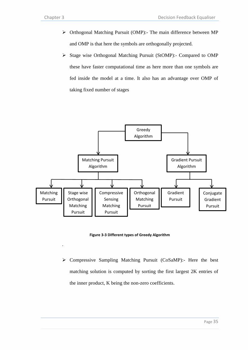
The greedy algorithms [17] as shown in Figure 3-3 are broadly classified as:-

Matching Pursuit

Matching Pursuit (MP):- It was first proposed by Mallat and Zhang in the

year 1993. It finds the best matching projection on multi-dimensional

data.

Chapter 3 Decision Feedback Equaliser

Page 35

Orthogonal Matching Pursuit (OMP):- The main difference between MP

and OMP is that here the symbols are orthogonally projected.

Stage wise Orthogonal Matching Pursuit (StOMP):- Compared to OMP

these have faster computational time as here more than one symbols are

fed inside the model at a time. It also has an advantage over OMP of

taking fixed number of stages

Figure 3-3 Different types of Greedy Algorithm

.

Compressive Sampling Matching Pursuit (CoSaMP):- Here the best

matching solution is computed by sorting the first largest 2K entries of

the inner product, K being the non-zero coefficients.

Greedy

Algorithm

Matching Pursuit

Algorithm

Gradient Pursuit

Algorithm

Matching

Pursuit

Orthogonal

Matching

Pursuit

Stage wise

Orthogonal

Matching

Pursuit

Compressive

Sensing

Matching

Pursuit

Conjugate

Gradient

Pursuit

Gradient

Pursuit

Chapter 3 Decision Feedback Equaliser

Page 36

Gradient Pursuit

Gradient Pursuit (GP): This algorithm computes the new estimate by

choosing gradient direction and step size while solving the least square

by MP. The main disadvantage of using this algorithm is the extra

computational cost of computing the step size.

Conjugate Gradient Pursuit (CGP): This algorithm computes the

conjugate of gradient direction and conjugate of step size.

From paper [17] that deals with the greedy algorithm, it is found that the reconstruction

error of StOMP and CoSaMP is significantly better than other algorithm such as MP,

OMP, GP and CGP algorithm in case of small sparity and more measurements. But if

we go for faster computation then gradient pursuit are better compared to matching

pursuit algorithm. Here we have used StOMP algorithm for finding the sparse solution.

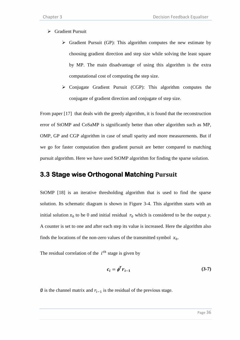
3.3 Stage wise Orthogonal Matching Pursuit

StOMP [18] is an iterative thresholding algorithm that is used to find the sparse

solution. Its schematic diagram is shown in Figure 3-4. This algorithm starts with an

initial solution 0 to be 0 and initial residual 0 which is considered to be the output y.

A counter is set to one and after each step its value is increased. Here the algorithm also

finds the locations of the non-zero values of the transmitted symbol 0.

The residual correlation of the stage is given by

(3-7)

is the channel matrix and is the residual of the previous stage.

Chapter 3 Decision Feedback Equaliser

Page 37

Figure 3-4 Schematic diagram of StOMP Algorithm

After computation of the residue, hard thresholding is performed to find the non-zero

location of the solution 0 . The thresholding is based on gaussianity. After that the

subset of the newly selected estimate are merged with the previously estimated solution.

Next the output is projected to find the estimate coefficient which is given by

(3-8)

Next the residue is updated using the equation

(3-9)

A stopping condition is checked, and if we do not reach the stopping condition then the

counter is incremented but if we reach to end then .

+

Matched

filter

Hard Thresholding

Set

union Projection

Interference

Construction

y 𝑟𝑖

𝑥

-

Chapter 3 Decision Feedback Equaliser

Page 38

3.4 System model

Here we consider the WCDMA based system model where K numbers of asynchronous

users are transmitting the modulated symbol [19]. The received noiseless signal is given

as

∑ ∑

(3-10)

where is the data transmitted by the user, being the power associated

by the user and being the symbol duration. The symbol represents the

convolution of the transmitted spreading waveform with the channel impulse response

which is given by

∑

(3-11)

Similarly if we consider the matrix model for the noise free channel then the equation is

given as

∑

(3-12)

Chapter 3 Decision Feedback Equaliser

Page 39

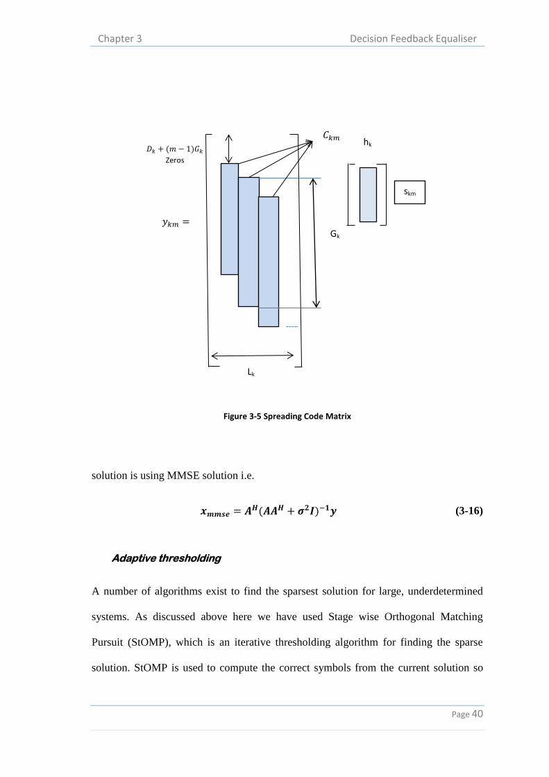
Here corresponds to the spreading code of user and symbol and is the

multipath fading channel of user. It is assumed that the user has a relative delay

of chip with respect to the reference of the received symbol. As shown in Figure

3-5, 1 values of the first column represents zeros followed by the

spreading code value and then the rest values are again filled by zeros so that it fills the

entire chips of the slot. Similarly the second column of the code matrix represents the

second multipath component with corresponding delay and spreading code and so on.

Considering noise, above equation becomes

(3-13)

[ ] (3-14)

(3-15)

H being the knocker diagonal matrix between identity matrix and the channel matrix

, being the symbols transmitted and is the additive white Gaussian noise.

3.4.1 Procedure

In decision feedback algorithm first we have to compute the correctly equalized

symbols. A solution that is close to the actual transmitted vector will give accurate

information for our decision feedback rule. The simplest way to compute the equalized

Chapter 3 Decision Feedback Equaliser

Page 40

Figure 3-5 Spreading Code Matrix

solution is using MMSE solution i.e.

(3-16)

Adaptive thresholding

A number of algorithms exist to find the sparsest solution for large, underdetermined

systems. As discussed above here we have used Stage wise Orthogonal Matching

Pursuit (StOMP), which is an iterative thresholding algorithm for finding the sparse

solution. StOMP is used to compute the correct symbols from the current solution so

𝑦𝑘𝑚 Gk

Lk

skm

hk 𝐶𝑘𝑚

𝐷𝑘 𝑚 1 𝐺𝑘

Zeros

Chapter 3 Decision Feedback Equaliser

Page 41

that the correct symbols should be feedback in order to reduce interference for the next

iteration. This is generally preferred as it has the advantage of having better

computational error.

First we compute the residual i.e. for iteration, if the initial solution is , that was

not correctly equalised in previous iteration, and then the residual can be given as

(3-17)

where Ai is the matrix that is obtained by leaving the column, from the matrix A that

corresponds to the correct symbols in previous iteration. is the observation in the

iteration, obtained by subtracting correctly equalised symbols in the previous iteration.

Initially i.e. in the first iteration, the dimension of solution 0 and error estimate 0 are

both dimensional, but as the iteration increases their size decreases.

Then we compute the estimate of error. The error estimate for iteration is

(3-18)

Here is a sparse, spiky signal added with noise and is given as

(3-19)

As we have obtained , now we have to compute a threshold which will help us to

determine which entries in e are small enough to be considered just noise and thus

should be fed back.

Chapter 3 Decision Feedback Equaliser

Page 42

It’s known that the maximum of the random Gaussian sequence is bounded by the given

equation as:

| [ ]| √ (3-20)

with high probability. So if we had an unknown spike function embedded in AWGN,

the right hand side of the above Equation (3-20 would be threshold that would

distinguish between the spike and the noise.

The level of sparsity is determined by the number of errors we make in our solution.

This number will be different in each iteration, so our threshold has to adapt

appropriately. We cannot know the number of error, that occurred in our current

solution but we need to know the level of sparsity of the actual error vector . We

obtain this estimate in the iteration as

|| ||

(3-21)

is the minimum distance among symbols for the used constellation. The Equation

(3-21 is used because the most likely errors are caused by mapping symbols into its

nearest neighbour symbols so the nonzero entries in is typically of size . As we

don’t know || || we consider || || = || || and obtain

|| ||

(3-22)

as the estimate of sparity of .

Chapter 3 Decision Feedback Equaliser

Page 43

The threshold for iteration is given as

√ (

)|| ||

√

(3-23)

Using the above threshold location of the correct symbols is computed so that they can

be subtracted in order to reduce interference. The symbols having estimated error less

than the threshold value are considered to be the correct values and represented by .

Thus each iteration the estimated error, residual value and threshold is computed and

the corresponding position of correct symbols is subtracted. As the number of iteration

increases the size of is reduced. The iteration process is repeated till all the values of

is over.

3.4.2 Algorithm

Step 1.

Estimate of the transmitted symbol is computed using the received symbol.

Step 2.

Residual is computed using the formulae

(3-24)

Step 3.

Estimated error is computed using

(3-25)

Chapter 3 Decision Feedback Equaliser

Page 44

Step 4.

Threshold value is computed using

√ (

)|| ||

√

(3-26)

Step 5.

Location of the symbols is found those have the estimated error value less than the

threshold value i.e. the position of correct symbols are computed.

Step 6.

Interference caused by the correct symbol is removed by using the equation

( ) (3-27)

Here ( ) corresponds to the matrix having all rows but only the columns having

index i.e. the correct symbol index.

Step 7.

The code matrix is updated by leaving the column that corresponds to the index set

.

Step 8.

If the index set is not exhausted then we move to step 1 else move to end.

Step 9.

End.

Chapter 3 Decision Feedback Equaliser

Page 45

3.5 Results and Discussion

The BER performance of WCDMA is evaluated for multipath channel. The BER

performance is evaluated by using Monte-Carlo simulation. This simulation is used to

compute the probability of error in the receiver. Here the symbols that are transmitted is

compared with the symbols that are received at the receiver section. If both are equal

means no error has occurred while they are not equal then the symbol is corrupted. Thus

BER is calculated using the formulae

(3-28)

Here we have used BPSK modulation. The simulation was performed by varying the

load in the system and also by varying the spreading factor. The results for different

channel were considered i.e.

Minimum Phase channel: This is the causal and stable channel that has all the

zeros lying within the unit circle. Zeros are the values in the system for which

the system tends to zero. This means all the zeros have a value less than 1. Here

we considered the channel to be 1 2.

Maximum phase channel: In this channel all the zeros lie outside the unit circle.

These are named so because they have maximum group delay of the set of

systems that have the same magnitude response. Here we have considered the

maximum channel to be 2.

Mixed phase channel: This type of channel has some of its zeros inside the unit

circle while others lying outside the unit circle. Thus, its group delay is neither

minimum nor maximum but somewhere between the group delay of the

Chapter 3 Decision Feedback Equaliser

Page 46

minimum phase and the maximum phase equivalent system. The channel values

were 1 2.

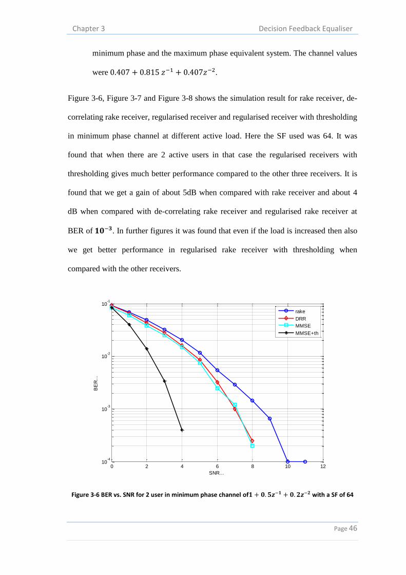
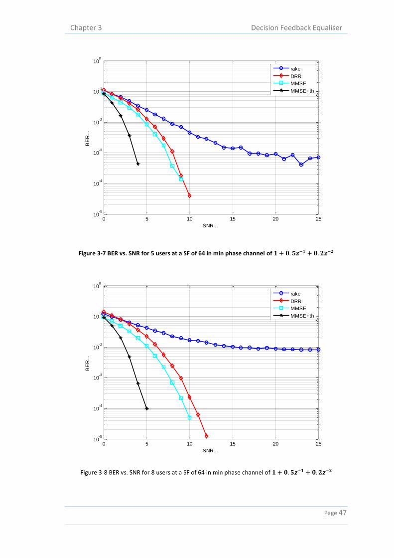
Figure 3-6, Figure 3-7 and Figure 3-8 shows the simulation result for rake receiver, de-

correlating rake receiver, regularised receiver and regularised receiver with thresholding

in minimum phase channel at different active load. Here the SF used was 64. It was

found that when there are 2 active users in that case the regularised receivers with

thresholding gives much better performance compared to the other three receivers. It is

found that we get a gain of about 5dB when compared with rake receiver and about 4

dB when compared with de-correlating rake receiver and regularised rake receiver at

BER of . In further figures it was found that even if the load is increased then also

we get better performance in regularised rake receiver with thresholding when

compared with the other receivers.

Figure 3-6 BER vs. SNR for 2 user in minimum phase channel of with a SF of 64

0 2 4 6 8 10 1210

-4

10-3

10-2

10-1

SNR...

BE

R..

.

rake

DRR

MMSE

MMSE+th

Chapter 3 Decision Feedback Equaliser

Page 47

Figure 3-7 BER vs. SNR for 5 users at a SF of 64 in min phase channel of

Figure 3-8 BER vs. SNR for 8 users at a SF of 64 in min phase channel of

0 5 10 15 20 2510

-5

10-4

10-3

10-2

10-1

100

SNR...

BE

R..

.

rake

DRR

MMSE

MMSE+th

0 5 10 15 20 2510

-5

10-4

10-3

10-2

10-1

100

SNR...

BE

R..

.

rake

DRR

MMSE

MMSE+th

Chapter 3 Decision Feedback Equaliser

Page 48

Figure 3-9 BER vs. SNR in maximum phase channel of at a spreading factor of 64 for 2 users

Figure 3-10 BER vs. SNR for 5 users in maximum phase channel of at a spreading factor of 64

0 2 4 6 8 10 12 1410

-5

10-4

10-3

10-2

10-1

SNR...

BE

R..

.

rake

DRR

MMSE

MMSE+th

0 5 10 15 20 2510

-5

10-4

10-3

10-2

10-1

100

SNR...

BE

R..

.

rake

DRR

MMSE

MMSE+th

Chapter 3 Decision Feedback Equaliser

Page 49

Figure 3-11 BER vs. SNR for 8 users in maximum phase channel of value at a Spreading factor of 64

Figure 3-12 BER vs. SNR for 2 users in mixed phase channel having the value of

at a spreading factor of 64

0 5 10 15 20 2510

-5

10-4

10-3

10-2

10-1

100

SNR...

BE

R..

.

rake

DRR

MMSE

MMSE+th

0 2 4 6 8 10 1210

-4

10-3

10-2

10-1

SNR...

BE

R..

.

rake

DRR

MMSE

MMSE+th

Chapter 3 Decision Feedback Equaliser

Page 50

Figure 3-13 BER vs. SNR curve for 5 user in mixed phase channel of value

with a spreading factor of 64

Figure 3-14 BER vs. SNR for 8 users at mixed phase channel having the value of

with a spreading factor of 64

0 5 10 15 20 2510

-5

10-4

10-3

10-2

10-1

100

SNR...

BE

R..

.

rake

DRR

MMSE

MMSE+th

0 5 10 15 20 2510

-5

10-4

10-3

10-2

10-1

100

SNR...

BE

R..

.

rake

DRR

MMSE

MMSE+th

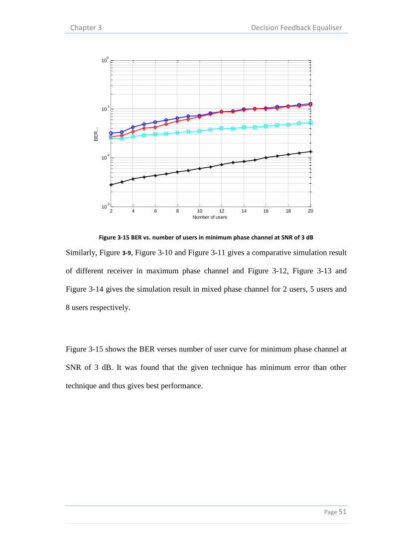
Chapter 3 Decision Feedback Equaliser

Page 51

Figure 3-15 BER vs. number of users in minimum phase channel at SNR of 3 dB

Similarly, Figure 3-9, Figure 3-10 and Figure 3-11 gives a comparative simulation result

of different receiver in maximum phase channel and Figure 3-12, Figure 3-13 and

Figure 3-14 gives the simulation result in mixed phase channel for 2 users, 5 users and

8 users respectively.

Figure 3-15 shows the BER verses number of user curve for minimum phase channel at

SNR of 3 dB. It was found that the given technique has minimum error than other

technique and thus gives best performance.

2 4 6 8 10 12 14 16 18 2010

-3

10-2

10-1

100

Number of users

BE

R..

.

Publication

Page 52

4

Conclusion

This thesis begins with the introduction to wireless communication and WCDMA,

reviewed the previously established receiver structures and introduced a new adaptive

thresholding technique. A nonlinear receiver was analysed in this thesis.

4.1 Summary

The first chapter deals with the introduction to wireless communication. It also deals

with the pro and cons of the communication. Then it gave a brief idea about the

different techniques used in different generation of wireless communication. This

chapter ends with the outline of the thesis.

Chapter 2 begins with introduction to WCDMA. It gives the different modulation

technique used in the uplink and downlink and the type of spreading code used for

transmission is shown. Then it gives a basic idea to the working of RR, its advantage

and its shortcoming.

Chapter 3 reviewed equalisers and different type of receiver structure. Initially the

linear and non-linear equaliser was discussed. A novel non-linear receiver was

Publication

Page 53

presented for WCDMA. A DFE with adaptive thresholding technique was used for

channel equalisation application. It used the StOMP algorithm for computing the sparity

error solution that gives an idea of feeding back symbols in case of DFE. Monte Carlo

simulation compared the receiver structure with the established linear and non-linear

receivers. The simulation results showed that the proposed receiver outperforms the

MMSE and other receiver techniques.

4.2 Conclusion

The thesis gives a brief idea about different equalisation algorithms for WCDMA

system. A de-correlating rake receiver was used in the receiver front end. This works

well only in the noise-free environment. A MMSE equaliser works better than the de-

correlating receiver in the noisy situation. At severe interference condition non-linear

equaliser is preferred as they lower the interference.

Here a decision feedback equalisation algorithm is used that works on adaptive

thresholding technique. The adaptive thresholding is used to find the sparsity of the

estimated error signal. This gives a theoretical frame work for the multiple feedback

symbol selection in each iteration which leads to a very fast convergence and also has

low computational complexity.

The simulation results shows that the work in this thesis gives much better performance

when compared with the linear equaliser such MMSE. We get a drastically improved

result when compared with the rake receiver, de-correlating rake receiver and

regularised rake receiver.

4.3 Limitation of Work

In this DFE technique, we are feeding back those symbols whose values are less than

the threshold value i.e. the location of the correct symbols are feedback. There is a

Publication

Page 54

problem to find the error symbols. Here we have assumed the error and the residual

value to be equal. A threshold value is used that helps in separating the error value and

the correct symbols is computed by using some of the estimation. Finding the threshold

is very crucial as, if the error symbol is fed back then the interference is increased. Here

lot of assumption are taken to find the different values. Here the simulation work is

done which is limited to software. There is a chance of variation of result in the real

world.

4.4 Future Work

The basic problem in developing a WCDMA receiver having better performance than

any linear receiver is that it should have some approximation technique. The techniques

should have the following constraints i.e. it should have simple receiver structure with

as low complexity as possible.

The given work in this thesis is a simple receiver and also gives good performance

when compared with the linear receiver. But it has a scope of having further work. It

has a chance of further improvement at low SNR region.

Now a day, a lot of compressed sensing and adaptive message passing (AMP)

algorithms have been used to improve the performance of iterative threshold algorithm

for computing the sparse solutions. There a chance of improving the performance at low

SNR by using other algorithms.

Publication

Page 55

Publication

S.Patel, S.K.Patra, ”Interference Suppression using De-correlating

rake receiver in WCDMA”, International Conference on Emerging

Trends in Computing, Communication and Nanotechnology, Tamil

Nadu, India,25-26 March ,2013.(Accepted and Presented)

References

Page 56

Bibliography

[1] T.S.Singhal, Wireless Communication, New Delhi: Tata McGraw Hills.

[2] Harri Holma and Toskala, WCDMA for UMTS, Finland: John Wiley and Sons, Ltd,

2004.

[3] Youngchul Sung, Yirang Lim,Lang Tong and Alle-Jan van der Veen, “Signal processing

Advances for 3G WCDMA:From Rake Receiver to Blind Techniques,” IEEE

Communication Magazine, vol. 47, no. 1, pp. 48-54, January,2009.

[4] H. Liu and M. Zoltowski, “Blind equalization in antenna array CDMA systems,” IEEE

Transaction Signal Processing, vol. 45, pp. 161-172, January,1997.

[5] M. Zoltowski, Y. Chen, and J. Ramos, “Blind 2D RAKE receivers based on space-time

adaptive MVDR processing for IS-95 CDMA system,” in Proc. 15th IEEE MILCOM, ,

Oct. 1996, Atlanta, GA, 1997.

[6] Y.Chen,M.D.Zoltowski,J.Ramos,C.Chatterjee and V.P.Roychowdhury, “Reduced-

dimension blind space-time 2-D Rake receiver for DS-CDMA communication sstems,”

IEEE Transaction Signal Processing, vol. 48, pp. 1521-1536, June 2000.

[7] Long Tong, Alle-Jan van der Veen, Patrick Dewilde and Youngchul Sung, “Blind De-

correlating Rake Receiver for Long Code WCDMA,” IEEE Transaction on Signal

References

Page 57

Processing, vol. 51, no. 6, pp. 1642-1655, June 2003.

[8] Jovana Ilic, Thomas Strohmer, “Sparity Enhanced Decision Feedback Equalization,”

IEEE Transaction on Signal Processing, vol. 60, no. 5, pp. 2422-2432, May 2012.

[9] Jovana Ilic, Thomas Strohmer and Raymoun Guan, “Decision Feedback Equalization

With Sparsity Driven Thresholding,” in IEEE CONFERENCE PUBLICATIONS,

Asilomar, 2010.

[10] J.G,Proakis, Digital Communication.

[11] Laurence B Milstein, “Wideband Code Division Multiple Access,” IEEE Journal on

Selected Areas in Communication, vol. 18, no. 8, pp. 1344-1354, August 2000.

[12] “Spreading Codes for Direct Sequence CDMA and Wideband CDMA Cellular

Networks,” IEEE Communications Magazine, vol. 36, pp. 48-54, September, 1998.

[13] Theodore.S.Rappaport, Wireless Communication, Noida: Pearson Publication, 2009.

[14] Wong and Lok, “ISI and Equalization.,” in Theory of Digital Communications, pp. 4.1-

4.24.

[15] Savo G. Glisic, Adaptive WCDMA:Theory and Practices, Chichester: John Wiley and

Sons Ltd., 2003.

[16] Simon Haykin, “Decision Feedback Equalisation,” in Digital Communication,

Daryaganj, John Wiley and Sons, 1988.

[17] Linfeng Du , Rui Wang , Wanggen Wan , Xiao Qing Yu , Shuai Yu, “Analysis on

References

Page 58

Greedy Reconstruction Algorithms Based on Compressed Sensing,” in IEEE

Conference, 2012.

[18] David L. Donoho, Member, Yaakov Tsaig, Iddo Drori and Jean-Luc Starck, “Sparse

Solution of Underdetermined Systems,” IEEE TRANSACTIONS ON INFORMATION

THEORY, vol. 58 , no. 2, pp. 1094-1121, 2012.

[19] “Channel Estimation and Multiuser Detection in Long-Code DS/CDMA Systems,” IEEE

JOURNAL ON SELECTED AREAS IN COMMUNICATIONS, vol. 19, no. 8, pp. 1476-

1487, August 2001.

[20] N.Anand Ratnesh, K.Balaji, J.V.Suresh,L.Yogesh, B.Anil Babu, “PERFORMANCE

ANALYSIS OF DS-CDMA RAKE RECEIVER OVER AWGN CHANNEL FOR

WIRELESS COMMUNICATIONS,” International Journal of Modern Engineering

Research, vol. 2, no. 3, pp. 859-863, June 2012.

Online resources

[21] http://www.kn-s.dlr.de/People/Haas/