Interactive signal processing documents

Interactive Signal Processing Documents

Malcolm Slaney

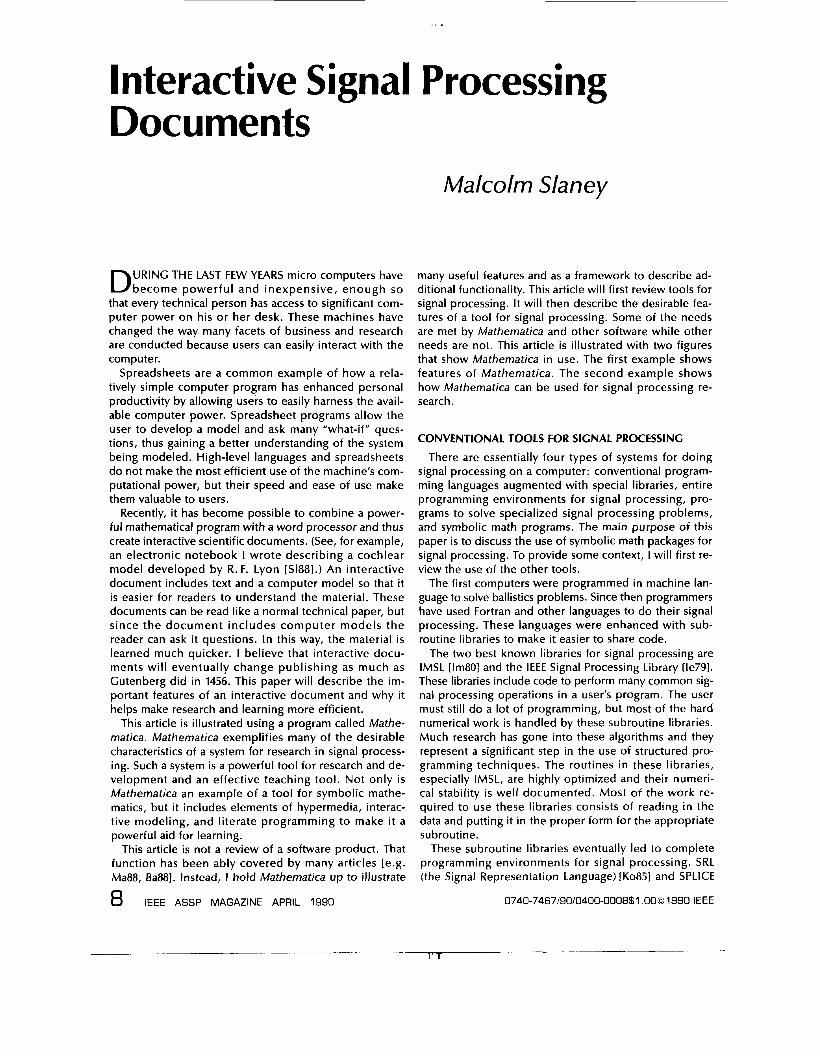
URlNG THE LAST FEW YEARS micro computers have D become powerful and inexpensive, enough so that every technical person has access to significant computer power on his or her desk. These machines have changed the way many facets of business and research are conducted because users can easily interact with the computer.

Spreadsheets are a common example of how a relatively simple computer program has enhanced personal productivity by allowing users to easily harness the available computer power. Spreadsheet programs allow the user to develop a model and ask many "what-if" questions, thus gaining a better understanding of the system being modeled. High-level languages and spreadsheets do not make the most efficient use of the machine's computational power, but their speed and ease of use make them valuable to users.

Recently, it has become possible to combine a powerful mathematical program with a word processor and thus create interactive scientific documents. (See, for example, an electronic notebook I wrote describing a cochlear model developed by R. F. Lyon [S1881.) An interactive document includes text and a computer model so that it i s easier for readers to understand the material. These documents can be read like a normal technical paper, but since the document includes computer models the reader can ask it questions. In this way, the material is learned much quicker. I believe that interactive documents will eventually change publishing as much as Gutenberg did in 1456. This paper will describe the important features of an interactive document and why it helps make research and learning more efficient.

This article is illustrated using a program called Mathe- matica. Mathematica exemplifies many of the desirable characteristics of a system for research in signal processing. Such a system is a powerful tool for research and de- velopment and an effective teaching tool. Not only i s Mathematica an example of a tool for symbolic mathematics, but it includes elements of hypermedia, interactive modeling, and literate programming to make it a powerful aid for learning.

This article is not a review of a software product. That function has been ably covered by many articles [e.g. Ma88, Ba881. Instead, I hold Mathematica up to illustrate

8 iEEE ASSP MAGAZINE APRIL 1990

many useful features and as a framework to describe additional functionality. This article will first review tools for signal processing. It will then describe the desirable features of a tool for signal processing. Some of the needs are met by Mathematica and other software while other needs are not. This article i s illustrated with two figures that show Mathematica in use. The first example shows features of Mathematica. The second example shows how Mathematica can be used for signal processing research.

CONVENTIONAL TOOLS FOR SIGNAL PROCESSING There are essentially four types of systems for doing

signal processing on a computer: conventional programming languages augmented with special libraries, entire programming environments for signal processing, programs to solve specialized signal processing problems, and symbolic math programs. The main purpose of this paper i s to discuss the use of symbolic math packages for signal processing. To provide some context, I will first review the use of the other tools.

The first computers were programmed in machine language to solve ballistics problems. Since then programmers have used Fortran and other languages to do their signal processing. These languages were enhanced with subroutine libraries to make it easier to share code.

The two best known libraries for signal processing are IMSL [Im80] and the IEEE Signal Processing Library [le791. These libraries include code to perform many common signal processing operations in a user's program. The user must still do a lot of programming, but most of the hard numerical work is handled by these subroutine libraries. Much research has gone into these algorithms and they represent a significant step in the use of structured programming techniques. The routines in these libraries, especially IMSL, are highly optimized and their numerical stability is well documented. Most of the work re- quired to use these libraries consists of reading in the data and putting it in the proper form for the appropriate subroutine.

These subroutine libraries eventually led to complete programming environments for signal processing. SRL (the Signal Representation Language) [Ko851 and SPLICE

0740-7467/90/0400-0008$1.00@ 1990 IEEE

I .

[My861 are examples of such specialized programming environments for signal processing. These systems are built on top of the Lisp programming language, and use object oriented techniques to make it easy for researchers to easily extend the environment.

Systems such as SRL and SPLICE are very powerful, but the i r non -s tandard p rogram m i ng m et hod0 I ogy (0 b ject- oriented Lisp) requires much effort to learn. In a sense, these tools are programmer friendly but not necessarily user friendly. This has limited their success.

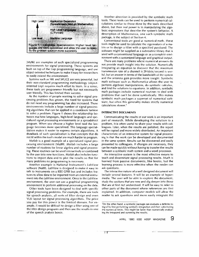
As the number of people wanting to solve signal processing problems has grown, the need for systems that do not need any programming has also increased. These environments include a large number of signal processing algorithms that can be applied in a cookbook fashion to solve a problem. Figure 1 shows the relationship between machine languages, high-level languages and specialized signal processing environments or a spreadsheet program. When you choose a higher level tool the language becomes more specialized. This language specialization makes it easier to express certain algorithms. A drawback of such specialization is that concepts that do not fit within the tool’s model are much harder to program.

Matlab is a good example of a specialized signal processing environment [Ma891. Matlab includes a large number of routines for linear algebra and signal processing. These routines can be used interactively or combined by the user into new functions. Matlab also includes functions to import data and to plot the results so that for many problems no programming is necessary.

Another example is National Instrument’s LabView software [Na891. LabView i s designed to make it easy to talk to instruments on a IEEE GPlB bus and includes features to allow data to be imported from an external instrument into the LabView environment. Once in the LabView environment, the user can use a graphical programming environment to perform additional processing on the data.

Other tools have been designed to deal with specific signal processing problems. For example, there are tools for speech analysis, all sorts of filter design and even VLSl layout for signal processing algorithms. The price you pay for this power i s the limited domain. For example, it would be difficult to design a filter using one of the filter design programs and then use the results in one of the speech analysis boxes.

~

I .

Another direction i s provided by the symbolic math tools. These tools can be used to perform numerical calculations similar to those done by the tools described above, but their real power is in manipulating the algebraic expressions that describe the system’s behavior. A description of Mathematica, one such symbolic math package, is the subject of Section 4.

Conventional tools are good at numerical math. These tools might be used to calculate the eigenvalues of a matrix or to design a filter with a specified passband. The software might be supplied as a subroutine library that i s used with a conventional language or as a complete environment with a customized language and graphical output.

There are many problems where numerical answers do not provide much insight into the solution. Numerically integrating an equation to discover that the maximum transmission rate of a channel is 29 kbits/second is useful, but an answer in terms of the bandwidth of the system and the antenna gain provides more insight. Symbolic math software such as Mathematica allows the user to perform algebraic manipulations, do symbolic calculus, and find the solutions to equations. In addition, symbolic math packages include numerical routines to deal with problems that can’t be done symbolically. This makes symbolic math packages a superset of numerical software, but often this generality makes strictly numerical calculations slower.’

INTERACTIVE D O C U M E N T S

Communicating the results of our work is an important part of research. While developing the solution to a problem, it i s often useful to share your results with colleagues. Later, when the results are polished, the report will be copied and more widely distributed. An important characteristic of an interactive system for signal processing is that the work can be developed and documented in the same system. Results can be discovered and easily presented to colleagues. If changes are necessary, they can be made quickly without having to transfer the results between a symbolic math system and a word processor.

An interactive system is the most effective means to teach and disseminate signal processing results. Much is learned from passive documents, like books, but the learning process is more effective when the reader can ask questions.

The interactive nature of a well designed document will include several features. It will be an example of hypermedia. The user will be able to explore the document, study the sections that are new and dig deeper into those that are at first not understood. It will be easy to refer to other parts of the document where references are first explained. In addition, computer models will allow the reader to ask questions and more easily integrate the

’On the other hand, a symbolic package can evaluate a definite integral by first performing symbolic integration and then substituting the numerical limits. This might be faster than numerically evaluat- ing the integrand and summing the results.

APRIL 1990 IEEE ASSP MAGAZINE 9

I .

new material with what is already known. Finally, a description of an algorithm must be explained in such a way that is easy for both a reader and a computer to understand. This i s known as Literate Programming, or the cre- ation of a document that is both a well written program and a well written paper.

The features of an interactive signal processing document as described above will be discussed in the remain- der of this section. But, these features are only part of a complete system. A symbolic math tool is just one com- ponent of the ideal system. A researcher will also need drawing programs to create graphics to explain the work and spelling checkers. These other components of a computer system are vital but are not discussed here.

Hypermedia

At one time information was passed from generation to generation via the story teller. This was inherently an interactive process, but it also limited the speed that information could be conveyed. By the middle ages publishing was well established. This increased the rate at which information could be disseminated, but it lost its interactive nature. During the last 10 years much effort has been expended to create interactive learning environments, and the results have been mixed. Perhaps the biggest im- pediment to their success has been their goal to create an all encompassing environment. This has brought with it the need for specialized and expensive computer systems, which are only available to a small number of users.

Most papers and books are designed to be read in a linear fashion. (Dictionaries and encyclopedias are examples of work that are meant to be accessed randomly.) The order of presentation is determined by the author, and the reader is expected to make the best of it. Some brows- ing is possible, but the paper media makes this inconve- nient. The reader is a passive part of the learning process.

Hypermedia i s often described as a solution to this problem [Ca88]. Using a computer, the reader can browse through a document and then quickly move to other parts based on what is read. Thus if a reader encounters a new concept, it might be accompanied by a button on the screen that will display more detailed information. In this way, the reader can fashion his or her own path through the material.

An interactive or electronic mathematical paper is a limited form of hypermedia. A paper is organized as a hi- erarchical document. Text, equations, output, and graphs are grouped into sections, and the entire paper organized into a hierarchy. Most papers have a tree-like structure, but the electronic version of a paper’s most detailed sections can be hidden from the user so as to make the presentation easier to follow. These hidden sections can be easily opened by the user and can be used to hide de- tails of the presentation, attempts that did not work, or test codes that isn’t strictly necessary for the presentation.

A system for creating and reading interactive signal processing documents will include a help facility to make it easier to understand the user’s problem. Since the help

10 IEEE ASSP MAGAZINE APRIL 1990

facility includes information about any function defined in the paper, this is a very simple form of hypermedia. A user can select any function name in the paper, select help, and read a short description of the function. When more information is needed about a function the system can take the reader to the point in the paper where the function is first defined.

Finally, an electronic document will be easily modified. Users can rearrange the report to make the presentation more natural for their background. In addition, users can add their own material. Since there does not have to be any difference in appearance between the original text and the “margin” notes, the document becomes person- alized for the reader.

Interactive Models

An interactive signal processing document extends the hypermedia concept by making each result an equation or computer model that the user can interact with. Since the system includes a computation engine, readers can change the model and see the effect. The results are shown graphically. By controlling the parameters of the model or system, the user can gain a better understanding of how it works.

An interactive system for signal processing is a useful research tool, but such a system can also be valuable to a reader trying to understand the results. A good instructor of piece of writing should guide the student to the same conclusions that were reached by the research. Hopefully, the learning process will be more efficient than the original research, but the same tools are useful in both cases.

An interactive signal processing document contains equations and computer models that the reader can ma- nipulate. In some cases, the reader will be content to change the parameters of a model and see how the results change. Other readers might want to study the model from a different angle. Perhaps due to a different educational background the reader will want to analyze the system response in the time domain instead of a frequency domain approach more natural to the original author. With a symbolic math package readers can apply the appropriate transformation and study the result in their preferred domain.

Users should be able to interact with a signal processing docment in two ways. A mathematical model can be modified to extend it into the reader’s own domain. For example, an interactive signal processing document I wrote to describe Lyon’s cochlear model includes an ele- mentary model of the outer and middle ears. A reader who is studying the outer or middle ears might want to substitute a more complete model of these organs to see the effect on the cochlear firing rate.

Direct manipulation is an important aid to learning. In many systems, the behavior is controlled by a numerical parameter. A paper describing such a system will probably include an equation describing the system’s behavior as a function of this parameter. But the user would have a much better feel for the behavior of the system i f there

~~

Filter Order Hz dB Response

3000 4000 -10. - 2 0 .

-30

-40. 4 - -50.

-60

-70

1 - -80

Filter Order

4 - 3 - 2- ‘p 1 -

-50 -60

-7 0

-80

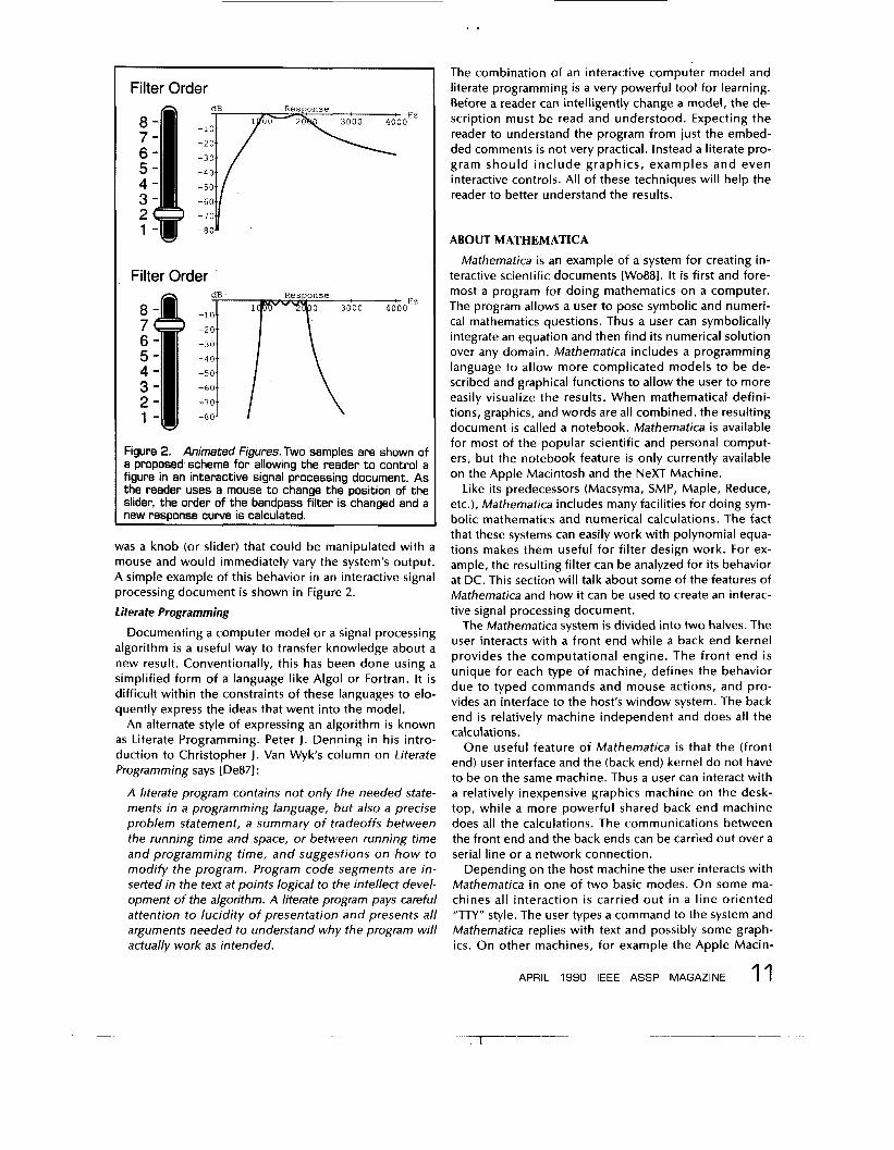
Figure 2. Animated F ih~es . Two samples are shown of a proposed scheme for allowing the reader to control a figure in an interactive signal processing document. As the reader uses a mouse to change the position of the slider, the order of the bandpass filter is changed and a new response curve is calculated.

was a knob (or slider) that could be manipulated with a mouse and would immediately vary the system’s output. A simple example of this behavior in an interactive signal processing document is shown in Figure 2.

Literate Programming

Documenting a computer model or a signal processing algorithm is a useful way to transfer knowledge about a new result. Conventionally, this has been done using a simplified form of a language like Algol or Fortran. It is difficult within the constraints of these languages to elo- quently express the ideas that went into the model.

An alternate style of expressing an algorithm is known as Literate Programming. Peter J. Denning in his introduction to Christopher J. Van Wyk’s column on Literate Programming says [De871 :

A literate program contains not only the needed state- ments in a programming language, but also a precise problem statement, a summary o f tradeoffs between the running time and space, or between running time and programming time, and suggestions on how to modify the program. Program code segments are in- serted in the text at points logical to the intellect devel- opment of the algorithm. A literate program pays careful attention to lucidity o f presentation a n d presents a l l arguments needed to understand why the program will actually work as intended.

The combination of an interactive computer model and literate programming is a very powerful tool for learning. Before a reader can intelligently change a model, the description must be read and understood. Expecting the reader to understand the program from just the embed- ded comments is not very practical. Instead a literate program should include graphics, examples and even interactive controls. All of these techniques will help the reader to better understand the results.

ABOUT MATHEMATICA Mathematica is an example of a system for creating in-

teractive scientific documents [Wo88]. It is first and fore- most a program for doing mathematics on a computer. The program allows a user to pose symbolic and numerical mathematics questions. Thus a user can symbolically integrate an equation and then find i ts numerical solution over any domain. Mathematica includes a programming language to allow more complicated models to be described and graphical functions to allow the user to more easily visualize the results. When mathematical defini- tions, graphics, and words are all combined, the resulting document is called a notebook. Mathematica is available for most of the popular scientific and personal computers, but the notebook feature is only currently available on the Apple Macintosh and the NeXT Machine.

Like its predecessors (Macsyma, SMP, Maple, Reduce, etc.), Mathematica includes many facilities for doing symbolic mathematics and numerical calculations. The fact that these systems can easily work with polynomial equations makes them useful for filter design work. For example, the resulting filter can be analyzed for its behavior at DC. This section will talk about some of the features of Mathematica and how it can be used to create an interactive signal processing document.

The Mathematica system is divided into two halves. The user interacts with a front end while a back end kernel provides the computational engine. The front end is unique for each type of machine, defines the behavior due to typed commands and mouse actions, and provides an interface to the host’s window system. The back end is relatively machine independent and does all the calculations.

One useful feature of Mathematica i s that the (front end) user interface and the (back end) kernel do not have to be on the same machine. Thus a user can interact with a relatively inexpensive graphics machine on the desk- top, while a more powerful shared back end machine does all the calculations. The communications between the front end and the back ends can be carried out over a serial line or a network connection.

Depending on the host machine the user interacts with Mathematica in one of two basic modes. On some machines all interaction i s carried out in a line oriented “ U Y ” style. The user types a command to the system and Mathematica replies with text and possibly some graphics. On other machines, for example the Apple Macin-

11 APRIL 1990 IEEE ASSP MAGAZINE

I .

M a t h e m a t i c a I n t r o d u c t i o n

This notebook is a short introduction to the features of Mathernatica. In the two notebooks accompanying this article the Mathernatica input is shown in a bold face Courier font and the Mathernatica output is shown in a n o r m a l C o u r i e r f o n t . See [Wolfram881 for more examples. Except for the two column output, what you see here is exactly the way Mathernatica shows output on the screen.

Numerical Calculat ions Mathernatica can be used like a calculator to do numerical arithmetic. Here is the numerical value of Pi calculated to 50 decimal places. N[Pi, SO] 3 . 1 4 1 5 9 2 6 5 3 5 8 9 7 9 3 2 3 8 4 6 2 6 4 3 3 8 3 2 7 9 5 0 2 8 8 4 1 \

9 7 1 6 9 3 9 9 3 7 5 1 Or Mathernatica can be used to numerically integrate an expression which can't be integrated symbolically. NIntegrata[Sin[Sin[xl I , {x, 0,l.O)l 0 . 4 3 0 6 0 6 1 0 3 1 2 0 6 9 0 6 0 4 5

Polynomial Manipulation Manipulating algebraic expressions is easy for Mathernatica. Here are some examples. First we multiply out the terms of an expression. Expand[ (x+l) (x+2) (x+3) A3 (x+4) 3 2 1 6 + 5 9 4 x + 639x2 + 350x3 + 1 0 4 x 4 +

We can then factor this equation to find the original expression.

1 6 x 5 + x 6

Factor[216 + 594*x + 639*xA2 + 350*xA3 + 104*xA4 + 16*xA5 + xA6]

(1 + x ) ( 2 + x ) ( 3 + x ) 3 ( 4 + x ) Solve[216 + 594*x + 639*xA2 +

350*xA3 + 1O4*xA4 + 16*xA5 + xA6==0,x]

{ ( x -> -11, { x -> -21 , { x -> - 4 } , ( x -> - 3 } , ( x -> - 3 ) , { x -> - 3 ) )

Here is a graph showing the behavior of this function as x varies between -5 and 0. Plot [ (x+l) (x+2) (x+3) A3 (x+4),

fxt-5,O)I;

C a l c u l u s Mathernatica knows a lot about calculus. After reading in Mathernatica's integration rules we can easily find the integral of x/( 1 -xA3). <<IntegralTables.m; Integrate [x/ (1-xA3), x]

- ( S q r t 131 1 t 2 x

S q r t [ 3 I ArcTan [-- - - - - - I )

- -__--_--_--_---_---------- - 3

L o g [ l - X I L o g [ l + x + x21 + --------------- ----------

3 6 Now let's differentiate this result and see if we get the original expression. Simplify[D[-(3A(1/2)*ArcTan[ (1 +

2*x) /3A(1/2) I) /3 - IIog[l - x]/3 + Log[l + x + xA21/6,x]1

X _----_ 1 - x 3

We can also find the series expansion of an expression. Seties[Exp[xlCos[4xl, {x,O,6)1

1 5 x 2 47 x 3 1 6 1 x 4

2 6 24 1 + x - ----- - _---- + ------ +

1 1 2 1 x 5 11 x 6

Fig. 3 Continued on next page

tosh, the front end allows the user to create what i s called a notebook. A Mathernatica notebook is much like a scientist's notebook since i t can contain data and thoughts about work in progress. But, Mathernatica notebooks are unique because in addition they contain computer models and even animations. The ability to create a live mathematical notebook is probably the feature that most distinguishes Mathernatica from other systems.


Notebooks contain text, equations and graphics. When a problem is first proposed, the notebook will reflect the steps actually used to carry out the calculation. It might contain false starts and notes understood only by the author. As the theory and calculations are refined, the notebook becomes more polished. Eventually, the notebook is cleaned up and the necessary text written so it can be distributed to colleagues. The finished notebook will

I .

Solv ing Equat ions Mathernatica can be used to solve simultaneous equations. Here is a simple example. Solve[fxA3+yA3==l, x+y==2),{x,y}]

6 - Sqrt[-61 12 + 2 Sqrt[-6] ) , { {x -> ------------ , -> ----------_---

6 12 6 + Sqrt[-61 12 - 2 Sqrt[-6]

1 , IX -> __---------- , -> --__---------- 6 12

The results are complex. G r a p h i c s Mathernatica can graphically show you the results of your calculations. Here is a plot showing the previous two equations. Note, there are no solutions for real values of x and Y. Plot [ { (1-x"3)~(1/3), 2-x), {x, -2,211

~ ~~~~~

Fig. 3 Continued

Data Analys is Mathernatica can be used to analyse the results of your experiments. Let's create a sample data set by adding random noise (uniform between 0 and 1) to a sine wave. data = Table[N[Sin[i/25] +

ListPlot [data] ; Random [ 1 1 , { i, 2 00 1 I ;

Now lets fit the data to a constant term (to get the mean of the random variable) and a sine and cosine of the appropriate frequency. Note that the term multiplying the cosine in the result is small compared to the factor multipying the sine. Fit[data, {l,Sin[x/25] ,Cos[x/25]),x]

X 0.499471 - 0.0565294 C O S [ - - ] +

25 X

0.9444936 Sin[--] 25

Programming by Example Rules can be added to Mathernatica to specialize it for your own problem domain. Here is an alternate definition of factorial. The first rules defines the stop condition. The second rule is the basic recursion to solve the problem. Fact[O] = 1

Fact[x-] := x Fact[x-1]

Fact [ 61 720

Here is an example of defining rules for simplifying logarithms in Mathernatica. log[a- b-] := log[a] + log[b] log[x y"2 21

log[xl + log[y21 + log[zl Now we can tell Mathernatica about powers log[x_"n-] := n log[xl

log[x/yI log[xl - log[yl

Notebooks have been written, for example, to compute the Laplace Transform of a symbollic expression.

contain explanatory text, symbolic and numerical models, and graphs and animations to explain the system and its solution. Figures 3 and 4 of this article and [SI881 are examples of notebooks in their polished form.

A notebook showing some of the capabilities of Mathe- matica i s shown in Figure 3 . Mathernatica can be used as a calculator, even with arbitrary precision, but its real

power comes from the symbolic functions. Equations can be integrated and differentiated, and algebraic manipulations can be done to put the result into a simpler form. The results can be plotted to help understand how the system works. A second, more complete example showing the use of Mathernatica in a signal processing application is shown in Figure 4.


Signal Processing Example This notebook is an example of using Mathernatica to describe continuous filter design. This notebook is fully functional. It includes some Mathernatica notation, but readers who are not Mathernatica users should have no problem understanding the notebook by just reading the text. See [Wolfram881 for an explanation of the special notation used by Mathernatica. Thanks to Ray DeCarlo at Purdue University for providing the original motivation to write this notebook.

There are a number techniques for designing higher order filters. This notebook will show how to design a Chebychev low-pass filter, and then how to transform the original low-pass poles into a band-pass filter. Section 1 of this example defines a number of functions used to work with filter polynomials. Section 2 describes the techniques to design Chebychev low-pass filters with a corner frequency of 1 radian per second (rps). Section 3 shows how to transform these generic low-pass filters into band-pass filters with arbitrary passbands.

1 - Continuous Fi l ter Functions Continuous time filters are described using polynomials of complex frequency, s . A filter's response function is evaluated along the imaginary axis by making the substitution s->I 2 Pi f (or j 2 Pi f i n conventional EE notation.) The following functions are used to evaluate the complex response of a filter for a real frequency (in cycles per second). Additional functions compute the gain, magnitude, and phase response of the filter. The expression f i l t e r can be an arbitrary function of the complex frequency, s . FilterGain [filter-, f-1 :=

FilterMag[filter-,f-] :=

Filterphase [filter-, f-] : =

FilterDb [filter-, f-] :=

PlotPoles [pl-] : =

ReplaceAll [filter, s -> I 2 Pi f 1 ;

Abs [FilterGain [filter, f ] ]

Arg [FilterGain [ f ilter, f ] ]

20 Log[lO,FilterMag[filter,f]]

ListPlot[Wap[{Re[#l ,Im[#] }h,pl], AspectRatio->Automatic];

The following function is used to display the frequency response of a continuous filter. (The plot starts at O.01Hz to avoid any problems with filters that have a zero at DC.)

FreqResponse[filter-, maxf-, opts,:{]] :=

Block[{response}, response =N[FilterDb[filter, f]] ; Plot[response, {f, .Ol,maxf),

AxesLabel->{" Hz", "dB''}, PlotLabel->'lResponse", optsl 1 ;

We define a similar function for displaying the frequency response of a filter as a function of radian frequency (omega or radians per second, rps). FreqResponseRadians[filter-, maxw-,

opts-:{}] := Block[{response},

response=N[FilterDb [filter, w/2/Bil 1 ;

Plot[response, {w, .Ol,maxw}, AxesLabel->{" RPS", "dB"], PlotLabel->"Response" , optsl I ;

Note, for each of these functions, there is a third optional argument which allows additional options to be set. We use this feature to pass special parameters to the Plot function. The frequency response of a fourth order filter is shown below. FreqResponseRadians[.197 sA2/ ((0.09 - 1.31 + S) (0.09 + 1.31 + S) (.12-1.81 + 8 ) (.12+1.81 + s ) ) , 4 ] ;

dB Response

- 2 c -

- a - 1 0

The AdjustGain function is used to modify a filter so that it has unity gain at any desired frequency. Ad justGain [ filter-, f-1

filter/FilterGain[filter,f] Higher order filters could be designed with Mathernatica using either rational polynomials or lists of poles and zeros. Rational polynomials would certainly be nicer since all intermediate results would look like filters. Unfortunately, we sometimes need to talk about individual poles and zeros, for example when doing partial fractions expansions. This is difficult if the filter is described as a

: =

Fia. 4 Continued on next page

polynomial. If a filter is described by its poles, zeros and gain, we can always regenerate the polynomial.

A list of polynomial roots are turned into a polynomial in s using this Mathematica expression. PolynomialFromRoota[roota~l :=

If [Length[roots] == 0, 1, Firat [Apply [Timea,

Map[~s-#~~,rootsllll PolynomialFromRoots[{4,2,1}] ( - 4 + s ) ( - 2 + s ) (-1 + s )

In this notebook we use a list to keep track of the zeros, poles, and gain of a filter. Functions that transform filters will take as input a list of three items and return a similar structure. We abbreviate the name of this structure to just GZP (Gain, Zeros and Poles.) The following function is then used to take one of these lists and transform it into a filter in the s-domain. Note that we have used the pattern matching facilities of Mathematica to pick out the three elements of the input list. FilterFromGZP[{gain-, zeros-,

polea-}] := gain * PolynomialFromRoots[zeros]/

PolynomialFromRoots[poles]//N

2 - C h e b y c h e v P o l y n o m i a l s The simplest higher-order filters to design are the Butterworth and the Chebychev. The poles of a Butterworth low-pass filter are arrayed so that the filter's response is smooth through most of its passband. As the frequency approaches the corner frequency the gain quickly falls off. In some cases this characteristic is an advantage because the gain between DC and the corner frequency is nearly flat.

For a given stopband or transition band specification, filters with a much smaller variation in gain in the passband can be designed using the Chebychev polynomials. Chebychev filters do not have a flat response in the passband but, as in Butterworth filters, the passband error can be made arbitrarily small.

The Chebychev polynomials are described by a . .

recursive relationship. A technique known as dynamic programming is used to remember lower order Chebychev polynomials so that they do not need to be recalculated each time they are used. ChebychevPoly[O] = 1 ChebychevPoly[l] = s ChebychevPoly [ n,] : =

ChebychevPoly [n] = Simplify [2 s ChebychevPoly [n-l]

- ChebychevPoly [n-211 ChebychevPoly [ 61 -1 + 1 8 s2 - 4 8 s 4 + 3 2 s 6

The poles of these polynomials are given by the following expression. This expression is a function of the desired order ( n ) and the maximum error (e ) in the passband. Chebychev [ n-, e-] : =

Table [Sin [Pi/2 (1+2k) /n] Sinh[ArcSinh[l/e] /n] +

Cosh [ArcSinh [ l/e] /n] , I Cos [Pi/2 (1+2k) /n]

{k,n, 2n-111 The C h e b y c h e v P o l e s function returns the location of the poles of a n- th order low-pass Chebychev filter with a cutoff frequency of 1 radian per second (rsp) and a maximum passband error of a m a x dB. It simply calls the C h e b y c h e v function descibed above, converting the passband error in dB into real gain. ChebychevPolea [n-, amax-] : =

ChebychevPoles [6,2] //N Chebychev[n, Sqrt 110" (amax/lO) -11 3

{ - 0 . 0 4 6 9 7 3 2 - 0 . 9 8 1 7 0 5 I, - 0 . 1 2 8 3 3 3 - 0 . 7 1 8 6 5 8 I, - 0 . 1 7 5 3 0 6 - 0 . 2 6 3 0 4 7 I, - 0 . 1 7 5 3 0 6 + 0 . 2 6 3 0 4 7 I, - 0 . 1 2 8 3 3 3 + 0 . 7 1 8 6 5 8 I, - 0 . 0 4 6 9 7 3 + 0 . 9 8 1 7 0 5 I}

As can be seen from the pole plot below, the roots of a Chebychev polynomial fall on an ellipse. maximum error in the passband is varied from

This plot shows the roots as the

10-l' (the ones that look most like a circle) to a passband error of 1 dB (the rightmost arc). PlotPolea [Flatten [Map [N [

ChebychevPoles [16, #I ] f i , {10"-10,10A-4,.l,l)]]];

Fig. 4 Continued on next page


I .

Fia. 4 Continued

. . . .

0 .

. . * 0.1

* .

. . . - 0'. 8- 0.. 6- 0': 4- 0-.2 .

. . .

. -0 :! . .

. I

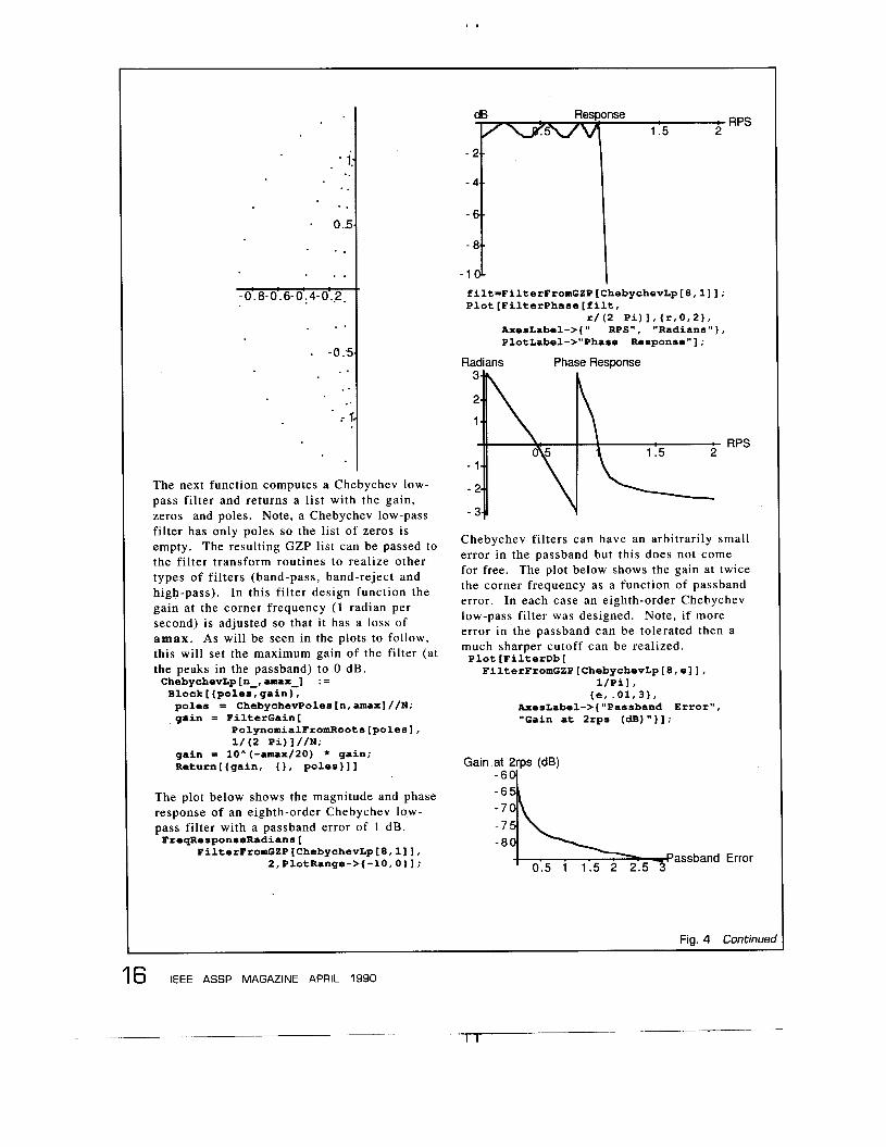
The next function computes a Chebychev low- pass filter and returns a list with the gain, zeros and poles. Note, a Chebychev low-pass filter has only poles so the list of zeros is empty. The resulting GZP list can be passed to the filter transform routines to realize other types of filters (band-pass, band-reject and high-pass). In this filter design function the gain at the corner frequency (1 radian per second) is adjusted so that it has a loss of amax . As will be seen in the plots to follow, this will set the maximum gain of the filter (at the peaks in the passband) to 0 dB. ChebychevLp In-, amax-] : = Block [ {poles, gain), poles = ChebychevPoles [n, amax] //N; gain = FilterGain[

PolynomialFromRoots[poles], 1/ (2 pi) I //N;

gain = 10^(-amax/20) * gain; Returnttgain, { I , poles)]]

The plot below shows the magnitude and phase response of an eighth-order Chebychev low- pass filter with a passband error of 1 dB. FreqResponseRadians[

FilterFromGZP[ChebychevLp[8,1]], 2,PlotRange->(-lO,O)];

: RPS dB Response 1.5 2

-1

filt=FilterFromGZP [ChebychevLp[B, 11 ] ; Plot [Filterphase [ f ilt,

r/(2 Pi)l,(r,0,2), AxesLabel->{I' RPS", "Radians"}, PlotLabel->"Phase Response"] :

Radians Phase Response

Chebychev filters can have an arbitrarily small error in the passband but this does not come for free. The plot below shows the gain at twice the corner frequency as a function of passband error. In each case an eighth-order Chebychev low-pass filter was designed. Note, if more error in the passband can be tolerated then a much sharper cutoff can be realized. Plot [FilterDb [

FilterFromGZP[ChebychevLp[8,ell, 1/Pil,

AxesLabel->{ "Passband Error", "Gain at 2rps (dB)"} 1 ;

{e, .01,3),

Gain at 2rps (dB)

- 6

- 7 d \

assband Error 0.5 1 1.5 2 2.5

3 - Bandpass Fi l ters Section 2 showed how to design a generic Chebychev low-pass filter. These low-pass filters can then be transformed into low-pass, high-pass, band-pass, and band-reject filters with arbitrary cutoff frequencies. This section will show how to transform a low-pass filter into a band-pass filter. We use the gain, zero, pole structure to keep track of the filter parameters.

A low-pass filter is transformed into a band- pass by specifying the location of the two corner frequencies. We make this transform by substituting the following expression for s into the normalized low-pass filter.

(s^2 + WOA2)

(B s ) s - - - - - - - - - - - -

In these expressions B is the difference (in radians) between the two edges of the passband and W O is the geometric mean of the freqencies at the edges of the passband. The function BpTransform is used to transform a single root of the normalized filter into two new roots due to the substitution above. (The extra root at zero is ignored for now.) BpTransf o m [ roots-, WO-, B-] : = N[ Flatten [ Map[{B # / 2 +

Sqrt[B"2#"2-4wOA2]/2,

Sqrt[B"2#A24wOA2]/2)&, B # / 2 -

roots] ] ]

BpTransform[ButterrorthPoles[3], 2Pi Sqrt [lo00 20001, 2Pi 10001

(-1104.8-6450.39 I, -2036.79+11891.8 I, -3141.59+8311.87 I, -3141.59-8311.87 I, -1104.8+6450.39 I, -2036.79-11891.8 I}

The function LpToBp transforms each of the poles and zeros in the original low-pass filter according to the BpTransform function. In addition, each zero in the original low-pass filter contributes a pole at zero, and, likewise, the original poles contribute a zero at DC. The difference between the number of poles and zeros tells us the number of additional roots at zero to add, and, in addition, extra factors of B to add to the gain.

LpToBp[{gain-, zeros-, poles-}, fpl-, fp2-] :=

Block[{rO, B, RootDiff, ExcessPoles, ExcessZeros},

WO = 2 Pi Sqrt[fpl fp21; B = 2 Pi (fp2 - fpl); RootDiff = Length[zeros] - If [RootDiff > 0,

Length [poles] ;

ExcessZeros = RootDiff;

ExcessPoles = -RootDif f; ExcessPoles = 0,

ExcessZeros = 01; {gain/B"RootDiff,

Join [BpTransforrn[ zeros, W O , B] ,

Join[BpTransform[poles,wO,B] , Table[O,{ExcessPolesfll,

Table[O,{ExcessZeros}]l}]

This transform is applied to a third order low- pass filter to determine a sixth order band- pass filter with a passband between 1 and 2kHz and a maximum passband error of 3dB. LpToBp[ChebychevLp[3,3], 1000,20OO]//N {-6.08732 10" - 1.25825 10101,

{ O . , O., 0.1, {-326.13 + 6478.28 I, -612.013 - 12157.1 I, -938.143 + 8836.1 I, -938.143 - 8836.1 I, -326.13 - 6478.28 I, -612.013 + 12157.1 I}}

The frequency response of this sixth order band-pass is shown below. FreqResponse [

FilterFromGZP [ LPTOBP [

ChebychevLp [3,3], 1000,2000] 1, 40001 ;

dB Resoonse 3000 4000

-10.

dB Response Hz 0

- 1

-2 - 3 - 4

- 5

- 6

- 7

Fig. 4 Continued


I .

One of the more useful features of a system like Mathe- rnatica is that it can be extended. Rules can be added or programs written to specialize the behavior of the program. In Mathernatica, rules are defined using a pattern matching language much like Prolog. On the left hand side of a rule the underscore character ( - ) indicates a wildcard position where any quantity can be substituted. Furthermore, the underscore character can be appended to a variable name to make a named wildcard variable. The pattern matching capability built into Mathernatica is very powerful. The simple expression

matches the function foo called with three arguments. The expression on the right hand side of the rule will be used with the appropriate substitutions whenever the variables a, b and c are used. A more complicated expression like

matches any time the factorial function is called with an integer argument. The matching expression can include arbitrary Mathernatica notation. For example,

can be used to pick apart a sum and define a new differ- entiation rule.

Mathernatica includes elements of a l l the important characteristics of a system for creating and exploring interactive signal processing documents. First, Mathernat- ica notebooks are organized hierarchically. Within a notebook, equations, paragraphs, mathematical results and graphics are each cells that can be grouped into larger cells. Cells can be hidden (or closed) in such a way that only the first line of a cell i s visible. From this information the reader can decide whether the rest of the cell needs further attention.

foofa-, b-, c- I

factorial[n- Integer]

difffa- + 6-1

know what parts of a Mathernatica expression to change. A graphical control, such as a slider, would make it possible for users, both novice and experienced, to directly control Mathernatica in a very intuitive fashion.

Readers of this article can get a sense of the readability of a notebook from the examples in Figures 3 and 4. A problem with Mathernatica is that the language i s new and probably unfamiliar to many readers. Notebooks should be written, much like mathematical papers [Kn89, p. 3, #131, so that the general flow can be understood by skipping the equations. A brief description of unusual syntax might be given the first time it is used. In this sense a notebook is no different from a normal paper.

All of these features of a notebook would not be inter- esting if notebooks could not be distributed. The essen- tial information in a notebook is conventional ASCII text, which i s easily moved through the email and computer networks. While only a small number of systems support the complete notebook concept all Mathernatica systems can understand the data and the mathematics contained in a notebook. Thus a reader with a version of Mathernat- ica without the full notebook capability can study the printed version and still try the examples.

Finally, Mathernatica is a commercial product that not everyone will be able to afford. Wolfram Research has put into the public domain a Mathernatica notebook reader. This notebook reader does not have any of Mathe- rnatica's mathematical ability but it does allow people to view a notebook and play the animations on any Macin- tosh computer. My own cochlear notebook has been published on paper and with a floppy disk containing the Mathematica notebook and this notebook reader to allow the material to have the widest possible distribution.

The help system in Mathernatica is an example of hypermedia. A user can select a function in a notebook and ask for more information. A new window appears con-

INTERACTIVE 'IGNAL PRoCESSING

taining the desired information. The system- would be even more useful if the user could ask about a function and be shown the appropriate part of the paper where the function is first defined.

An interactive notebook extends the hypermedia concept because a function i s not just a collection of sym- bols, but, more importantly, has a mathematical meaning. Using a function in a notebook not only implies a link back to the original definition, but the usage implies a specific mathematical operation. Hopefully, these "smart links" will be more prevalent in the future.

Most symbolic math packages are interactive. A Mathe- rnatica notebook is unique, though, because the writer can guide the reader by suggesting areas to explore. A Mathernatica notebook should encourage the reader to try new ideas. Mathernatica can show the results as equations, a figure or even an animation.

It is unfortunate that a Mathernatica notebook does not support direct manipulation. Currently, Mathernatica notebooks have to be carefully written so that the reader does not have to understand much of Mathernatica to

The benefits of interactive signal processing documents described here do not come for free. Certainly the design and writing of such a document takes more thought and care than the types of papers we are used to writing. And, when the interactive document is done there are no easy ways to disseminate the bits. Both of these problems should diminish as people become more familiar with this new medium for research and publishing.

Designing an interactive document is not easy. But, I believe the effort is worthwhile since writing an interactive mathematical document becomes as much a learning experience as reading it. Trying to teach new material i s often the best way to learn it. By preparing an interactive document, one is forced to study the material as a reader, and by having a tool such as Mathernatica it i s possible to explore more of the subject area. In addition, when a common system is used to research and present a new result, the effort in creating an interactive document i s minimized.

On the other hand, it i s hard to believe that any one system will solve everybody's problems. Instead, it will

probably be best if a user can mix a tool for filter design from one vendor with a special purpose accelerator from another to make the most efficient research and learning environment.

Publishing notebooks and other forms of electronic documents are not easy. Magazines and journals usually used to disseminate research results have evolved efficient mechanisms and designs to effectively communi- cate the printed word. But, a single floppy, or other form of electronic media, can cost more than the magazine it accom pan ies.

One of the more successful schemes for electronic publishing is based on the international computer networks. Jack J. Dongarra at Argonne Labs maintains an electronic mail system for distributing many large numerical software packages [Do87]. Users can send electronic requests to a special address and receive more information or the software by return mail. Another scheme is to broadcast the software on one of the computer bulletin boards. This i s commonly done, for example, on the Usenet bulletin board comp.sources [Qu86].

Unfortunately, not everyone has access to the computer networks. A recent issue of the Communications of the ACM [Ca88] included an advertisement for floppy disks containing hypermedia examples. My own report on the implementation of a cochlear model [SI881 was published as a technical report so it could be accompanied by a floppy disk containing the Mathematica notebook.

An additional problem is that an electronic document is not as convenient as a magazine or a book. Curling up with a computer will probably never have the same ap- peal as curling up with a good book, but the next genera- tions of portable computers should make this easier. My own notebook was designed so that it can be read as a normal paper but without all the benefits of an electronic document.

Finally, there i s the issue of notation. Within any one technical area, for example, signal processing or high en- ergy physics, the notation is well established, but it often differs widely between areas. Even a concept as simple as an integral is written in many different ways with marks to indicate different flavors of integration.

Mathematica solves this problem by defining a new language based on the ASCII alphabet. Wolfram has ex- changed the rich notation that scientists and mathemati- cians have evolved through the ages for a very precise functional notation. For example, to find the Laplace Transform of a function of t i n terms of the complex variable s one writes

Other programs, such as Milo, by a company called Para- comp, use a more conventional mathematical notation, but their knowledge of mathematics is limited. Perhaps the best solution is to allow the user to define graphical templates, which are used when the system wants to translate its internal representation into something to be displayed to the reader. This st i l l leaves the mathematical input problem to be solved.

Laplacer fR1, t, SI

ACKNOWLEDGEMENTS

I would like to thank a number of people for help with this article. The0 Gray and Nancy Blachman at Wolfram Research have been invaluable in helping me master Mathematica. They have both been very understanding when I tried to use Mathematica in ways that were never envisioned. I would also like to thank Richard F. Lyon, Neenie Billawala, Monica Ertel, Pam Lau and Nancy Tague for their help in producing the notebook [SI881 that led to this article. Finally, I appreciate the comments and suggestions my colleagues at Apple and the anonymous re- viewers have made to help improve this article.

Macintosh i s a trademark of Apple Computer, Inc., NeXT is a trademark of Next Computer, Mathematica is a trademark of Wolfram Research, Inc., LabView is a trademark of National Instruments, Matlab is a trademark of Mathworks, and Milo is a trademark of Paracomp.

REFERENCES

Ba881 John Barwise, “Computers and Mathematics,” Notices of the American Math Monthly, Vol. 35,

Ca881 Special Issue on Hypertext, Communications of the ACM, July 1988.

De871 Peter J. Denning, “Announcing Literate Program- ming,” Communications o f the ACM, Vol. 30, No. 7, July 1987, p. 593.

[Do871 Jack J. Dongarra and Eric Grosse, “Distribution of Mathematical Software via Electronic Mail,” Communications o f the ACM, Vol. 30, pp. 403- 407, May 1987.

[le791 Programs for Digital Signal Processing, IEEE Press, John Wiley and Sons, 1979.

[Im801 IMSL Library Reference Manual, IMSL Inc., Hous- ton, TX, 1980.

[Kn891 Donald E. Knuth, Tracy Larrabee, Paul M. Roberts , Mathematical Writing, MAA Notes No. 14, The Mathematical Association of Amer- ica, 1989.

[Ko85] Gary Kopec, “The Signal Representation Lan- guage SRL,“ IEEE Transactions on Acoustics Speech and Signal Processing, Vol. ASSP-33,

[Ma881 “Enter Mathematica ,” MacUser, pp. 199-216, November 1988.

[Ma891 Matlab ‘’ for Macintosh Computers, The Math- Works, Inc. South Natick, MA, 1989.

[My861 Cory S. Myers, “Signal Representation for Sym- bolic and Numerical Processing,” Research Labo- ratory of Electronics, Massachusetts Institute of Technology, Technical Report No. 521, Aug. 1986.

[Na89] LabVIEW, Scientific Software for the Macintosh, National Instruments Corporation, Austin, TX, 1989.

[Qu861 John S. Quarterman and Josiah C. Hoskins, “No- table Computer Networks,” Communications of the ACM, Vol. 29, Oct. 1986, pp. 932-971.

NO. 9, pp. 1333-1349, NOV. 1988.

NO. 4, pp. 921-932, August 1985.


1 ’ I

[SI881 Malcolm Slaney, "Lyon's Cochlear Model," Apple Computer Technical Report #13, Apple Com- puter, Inc., Cupertino, CA 1988. (This report i s available from the author or the Apple Corporate Library.)

[W0881 Stephen Wolfram, Mathematica: A System for Doing Mathematics by Computer, Addison Wesley, 1988.

Malcolm Slaney is a researcher in the Ad- vanced Technology Group at Apple Com- puter studying issues in auditory perception. In addition to his interests in electronic publishing, he is studying cochlear modeling, sound separation, and speech recognition in natural environments.

Malcolm received his Ph.D. from Purdue University for his work on algorithms for acoustic and microwave tomography. H e

wrote, with A. C. Kak, "Principles of Computerized Tomographic Imaging," which was published by IEEE Press in 1988.

RANDOM SIGNAL ANALYSIS with Random Processes and Kalman Filtering

Offers a complete survey of random signal analysis, in- cluding probability and random variable fundamentals, random processes, signal analysis, and optimal filter theory.

The ILP package includes a study guide, a floppy disk containing text, examples, and quizzes, a final exam, and a textbook, Probability, Random Variables, and Random Signal Princi les, Second Edition, by P. Z. Peebles, Jr., McGr aw-Hii, 1987.

Random Signal Analysis is IEEE member priced at $249 ($498 non-member). For a full description of the program and complete ordering information, call IEEE today at 1- 201-562-5498 .... Telex: 833233.. ..Fax: 1-201-981-1686.

Or write to: IEEE Educational Activities 445 Hoes Lane PO Box 1331 Piscataway, NJ 08855-1331


GET RESEARCH RESULTS

WITH INTEGRATED SIGNAL ANALYSIS

You want to spend your time interpreting results not programming research tools. Integrated Signal Analysis (ISA) is the only software system that gives you a ready-to-use arsenal of linear and higher-order spectral analysis tools.

F A S T E R

FEATURES

Birpectrum, Bicoherency, Sicorrelation Quadratic lkansfer Function Quadratic System Coherency Preconditioning Digital Filters Phase-Sensitive Complex Demodulation

. Wsvenur,iber-~2equency Spectrum Fluctuation-Induced Transport . FFT (any leugth) . Standard Spectrum and Carrelatiou . Linear Transfer finction

SOME APPLICATION AREAS rn Plasma Physics e Fluid Dynamics e Nonlinear Radar

Underwater Acoustics Nonlinear Ship Dynamics Oceanography Offshore Technology Nonlinear Modal AnaJyais Biomedical Research

ISA uses a layered modular structure so you can customize it to fit special needs. The application modules are coded in standard FORTRAN-77 for portability, Plotting features are already coordinated with the signal processing modules. Publication-quality graphic output is on NCAR (National Center for Atmospheric Research) GKS-compatible graphics system. ISA runs on VMS and 4.3BSD on DEC VAX family computers.

aD 1-800-366-9081

For more informstion, p l e s e call or write INTEGRAL SIGNAL PROCESSING, INC.

7719 Wood Hollow Dr., #219, Austin, TX 78731, (512) 346-1451

Get all the aesign gols you need to build your filters. And all the analysis and simulation tools you need to test them. MONARCH.. . The power package for DSF

3 Architectures Fixed / Floating Point Support State-Variable Modeling Pole-Zero Description ANALYSIS

Interactive Signal Laboratory 100+ DSP / Math Functions Signal & Matrix Operations

User-Defined Macros

30 doy money-bock guarantee

Customize with advanced DSP packages: pp Code Gen and Board Support, Additional Architectures, Spectral Estimation,