Embed Size (px)
Citation preview

arX
iv:1
202.
2240
v2 [
mat
h.K
T]
26
Oct
201
2
INTEGRAL COHOMOLOGY OF RATIONAL PROJECTION
METHOD PATTERNS
FRANZ GAHLER, JOHN HUNTON, AND JOHANNES KELLENDONK
Abstract. We study the cohomology and hence K-theory of the ape-riodic tilings formed by the so called ‘cut and project’ method, i.e., pat-terns in d dimensional Euclidean space which arise as sections of higherdimensional, periodic structures. They form one of the key families ofpatterns used in quasicrystal physics, where their topological invariantscarry quantum mechanical information. Our work develops both a the-oretical framework and a practical toolkit for the discussion and calcu-lation of their integral cohomology, and extends previous work that onlysuccessfully addressed rational cohomological invariants. Our frameworkunifies the several previous methods used to study the cohomology ofthese patterns. We discuss explicit calculations for the main examplesof icosahedral patterns in R3 – the Danzer tiling, the Ammann-Kramertiling and the Canonical and Dual Canonical D6 tilings, including com-plete computations for the first of these, as well as results for many ofthe better known 2 dimensional examples.
Contents
1. Introduction 22. Projection patterns, their spaces and cohomology 43. Homological algebra for cut and project schemes 83.1. C-topes and complexes 83.2. A homological framework 103.3. Exact sequences for pattern cohomology 114. Geometric realisation 145. Patterns of codimension one and two 205.1. Codimension 1 205.2. Codimension 2 215.3. Example computations 246. Patterns of codimension three 276.1. Rational computations 316.2. Torsion and the integral computations 336.3. Codimension 3 examples with icosahedral symmetry 366.4. K-theory and general codimension 38
Date: July 18, 2018.Key words and phrases. aperiodic patterns, cut and project, model sets, cohomology,
tilings.
1

2 FRANZ GAHLER, JOHN HUNTON, AND JOHANNES KELLENDONK
7. Appendix: realisation of H∗(Ω) as group (co)homology 40References 41
1. Introduction
This work considers one of the key families of aperiodic patterns used inquasicrystal physics. We develop both a theoretical framework and a prac-tical toolkit for the discussion and calculation of the integral cohomologyand K-theory of these patterns. Our work extends previous results whichsuccessfully addressed only their rational cohomology [20, 21, 29] and it pro-vides a unified treatment of the two apparently distinct approaches [20, 21]and [29] studied so far in the literature. The patterns we consider are pointpatterns in some d-dimensional Euclidean space Rd that arise as sections ofhigher-dimensional, periodic structures, variously known as model sets, cut& project patterns or just projection patterns [35]. By a standard equiva-lence, such point patterns may also be considered as tilings, coverings of Rd
by compact polyhedral sets meeting only face to face. The Penrose tilingin 2 dimensions is perhaps the best known example, but the class is huge(indeed, it is infinite) and today forms the principal set of geometric modelsfor physical quasicrystals; see, for example, [42]
To any point pattern or tiling P in Rd a topological space associated toP , called the hull or tiling space Ω of P , may be constructed. In short,this is a moduli space of patterns locally equivalent to P . Under standardassumptions (certainly satisfied by the class of patterns we consider), Ω isa compact, metrisable space, fibering over a d-torus with fibre a Cantor set[21, 38]. Much progress during the last 20 years or more in the study ofaperiodic patterns has developed through the study of these spaces, whichcan by analyzed via standard topological machinery such as cohomologyor K-theory. Major results include the Gap Labeling Theorem [7, 8, 9,10, 11, 30], the deformation theory of tilings [12, 31, 38] and the work onexact regularity of patterns and the homological Pisot conjecture [5, 40].For a short introduction to the topology of tiling spaces and some of thegeometric and physical benefits of understanding their cohomology, we directthe reader also to [39].
It is a general truth that by writing any tiling space Ω as a Cantor bundleover a d-torus, one can realise the Cech cohomology of Ω as the groupcohomology of Zd with coefficients derived from the structure of the fibreand the holonomy of the bundle. In general, however, one has little holdover either the fibre or the holonomy, but, as was realised in [20, 21], thereis a large class of projection tilings for which a practical description canbe obtained. This class contains the so-called canonical projection tilings,and was later called the class of almost canonical tilings [28]; we presentthem formally in the next section. (It is interesting to note that this is also

INTEGRAL COHOMOLOGY OF RATIONAL PROJECTION METHOD PATTERNS 3
the class of tilings whose asymptotic combinatorial complexity can be easilyobtained [28].)
In [20, 21] Forrest, Hunton and Kellendonk effectively provided a methodfor the computation of the rational cohomology of the spaces Ω of almostcanonical tilings. A related, but non-commutative approach, describing theK-theory of crossed product algebras associated to these tilings, was given byPutnam in [37]. Results similar to [21] for a smaller class of projection tilings,produced from an apparently rather different perspective, were obtained byKalugin in [29] who gave a shape equivalent approximation to Ω by a finiteCW complex (though that terminology was not used in [29]).
However, a key feature of the interpretations of all these works at thetime was the assumption that the cohomology and K-theory of these pat-tern spaces would be free of torsion, and thus integral computation wouldfollow from just working with rational coefficients and counting ranks ofvector spaces. This turned out not to be the case (and, unfortunately, somestatements about and referring to the torsion freeness of cohomological orK-theoretic invariants in [18, 20, 21] are wrong). This was shown, for exam-ple, by Gahler’s counterexamples [23] obtained through extensive machinecomputation for certain 2 dimensional patterns which arise as both pro-jection and substitution tilings. The substitution structure allowed a yetfurther approach to computation via the method of Anderson and Putnam[2], though even for relatively modest 2 dimensional examples this methodis stretched to the limit of accessible computation. Nevertheless, exam-ples computed, in particular the Tubingen Triangle Tiling (TTT) [3, 32],demonstrated that the integral cohomology could be far more complicatedthan had previously been thought, and this formed the stimulus of our workhere. We understand that the existence of torsion, not appreciated at thetime when [8, 10, 11, 30] were written, may cause problems with some ofthe arguments used in the published proofs of the Gap Labeling Theorem.
Given the consequent complexity of the cohomology H∗(Ω), its completedescription for projection method patterns is beyond the scope of the tech-niques of any of [2, 20, 21, 29] for all but the simplest examples.
In this paper we present techniques to address this. In Section 3 weintroduce a set of ideas from homological algebra that can be applied fordiscussing the bundle structures associated to these patterns. As a furtherconsequence, the generality of the framework developed allows us to unifythe approaches of both [20, 21] and [29], and this point has computationaladvantages when we turn in the final section to the discussion of the morecomplex examples.
In Section 4 we give a geometric interpretation of almost canonical pro-jection patterns whose cohomology is finitely generated and which satisfyone further assumption. This is inspired by and is an analogue of a certainkey assumption made in Kalugin’s approach [29]. Patterns which enjoy thisgeometric interpretation we term rational projection method patterns; theyform the central class for which we compute integer cohomology in the final

4 FRANZ GAHLER, JOHN HUNTON, AND JOHANNES KELLENDONK
section. Section 4 ends with a complete description of the cohomology of arational projection pattern in terms of data coded in the cohomology of aninclusion of a certain finite CW complex A in an ambient torus T.
It is these two new ingredients, the geometric interpretation of Section 4and the homological framework of Section 3, which give us tools to analysisinteger cohomologyy for examples beyond the ready scope of any of theprevious works in the field.
The final sections of the paper turn to the actual computation of exam-ples. The complexity of the computation of the cohomology of a projectionpattern increases with the so-called codimension of the pattern. In Section5 we give a complete description of the cohomology of rational projectionpatterns of codimension 1 and 2, together with details of many of the mainexamples and an outline of the machine methods used to compute them.Strictly speaking, the results of this section are accessible with the oldertechniques of [20, 21, 29], but the section provides the necessary foundationfor the new and more complex work of Section 6 which considers the codi-mension 3 examples and, briefly, the cohomology and K-theory of generalcodimension rational patterns. We note that the physically interesting ra-tional projection patterns (i.e., those in dimension up to 3) arise only fromcodimension 1, 2 or 3 schemes. We compute explicitly the cohomology ofthe Danzer tiling [14], and much of the cohomology of three other 3 dimen-sional, icosahedral patterns, those of Ammann-Kramer [33], the canonicalD6 and dual canonical D6 patterns [34].
Some of these results and ideas were announced in [25] (though the readershould note that there are some errors in the computation of the torsioncomponent of H3(Ω) published in [25] – see Section 6.3 for details), but theframework and techniques presented here have developed considerably sincethat note.
Acknowledgements. The first author was supported by the German Re-search Council (DFG) within the CRC 701, project B2. The second authoracknowledges the support of study leave granted by the University of Leices-ter, and the hospitality of Universite de Lyon. The third author acknowl-edges the financial support of the ANR SubTile.
2. Projection patterns, their spaces and cohomology
We begin by describing the types of patterns we consider, and in so doingset up our notation. The contents of this section are mostly a brief summaryof the set-up and foundational results of [20, 21]; the reader should consultthose sources for further detail and discussion. We start by listing the dataneeded for a model set, or cut and project pattern.
Definition 2.1. A cut & project scheme consists of a euclidean space Eof dimension N containing a discrete cocompact abelian group (or lattice)
Γ. There is a direct sum decomposition E = E‖ ⊕ E⊥ with associatedprojections π‖ : E → E‖ and π⊥ : E → E⊥. We assume E‖ and E⊥ are in
INTEGRAL COHOMOLOGY OF RATIONAL PROJECTION METHOD PATTERNS 5
total irrational position meaning that π‖ and π⊥ are one to one and withdense image of the lattice Γ. Denote by d, respectively n, the dimensions ofE‖ and E⊥, so N = d+n. We call d the dimension of the scheme, and n itscodimension. Finally, we have also an acceptance window or atomic surfaceK, a finite union of compact non-degenerate polyhedra in E⊥. We denote by∂K the boundary ofK, which consists of a finite union of (n−1)-dimensionalfaces fi.
For convenience we denote by Γ‖ and Γ⊥ the images π‖(Γ) and π⊥(Γ).
These are both rank N free abelian subgroups of E‖ and E⊥ respectively.
Definition 2.2. Given a cut & project scheme, we define the associatedpoint pattern P as the set of points in E‖
P = π‖(γ)|γ ∈ Γ : π⊥(γ) ∈ K
or equivalently as
P = E‖ ∩ (Γ−K).
There are a number of variations in the way cut and project patterns canbe viewed. In [21] the viewpoint was taken that these patterns arise as pro-jections of point patterns within strips E‖+K. Kalugin in [29] uses the sec-tion method by means of which these patterns arise as intersections betweenE‖ and a Γ-periodic arrangement of sets. In [20] the dual method using La-guerre complexes was adopted, which is more elegant for some tilings suchas the Penrose tilings. The reader can consult Moody’s work, for example[35], for a wide ranging discussion of these patterns.
A cut and project scheme in fact defines a whole parameterised family ofpoint patterns in E‖.
Definition 2.3. For each point x ∈ E define the point set
Px = π‖(γ)|γ ∈ Γ : π⊥(γ + x) ∈ K
= E‖ ∩ (Γ + x−K).
Note that the pattern Px depends only on the class of x in E/Γ = T, anN -torus. In fact Px = Py if and only if x− y ∈ Γ.
Definition 2.4. We define the set S of singular points in E by
S = x ∈ E : π⊥(x) ∈ ∂K + Γ⊥ = E‖ + Γ + ∂K .
Denote by NS its complement, the set of nonsingular points.
It is well known that, for any x, the pattern Px is aperiodic, i.e., thatPx = Px + v only if v is the zero vector, and is of finite local complexity,meaning that, up to translation, for each r > 0 there are only a finitenumber of local configurations of radius r in Px. If x ∈ NS then Px satisfiesthe additional property that for each finite radius r there is a number Rsuch that any radius r patch of Px occurs within distance R of any givenpoint of E‖, a property known as repetitivity. We note further that if x

6 FRANZ GAHLER, JOHN HUNTON, AND JOHANNES KELLENDONK
and y are both nonsingular points, then the patterns Px and Py are locallyindistinguishable in the sense that each compact patch of one pattern occursafter translation as a patch in the other. Although these are importantproperties and motivate interest in understanding and characterising cut andproject patterns, they will not generally play a very explicit role in the workwhich follows, though they implicitly account for many of the topologicalproperties of the space Ω we will shortly introduce and is the main topic ofthe article. Again, see [35] for further introduction and discussion of theseproperties.
The cohomology of point patterns which we investigate here is the Cechcohomology of an associated pattern space. Suppose for simplicity that0 /∈ S.
Definition 2.5. The pattern space Ω of P = P0 is the completion of thetranslates of P with respect to the pattern metric, defined on two subsetsP,Q ⊂ E‖ by
d(P,Q) = inf
1
r + 1
∣
∣
∣
∣
there exists x, y ∈ B 1
r
with(
Br ∩ (P − x))
∪ ∂Br =(
Br ∩ (Q− y))
∪ ∂Br
.
Here Br is the closed ball around 0 of radius r in E‖. In essence this metricis declaring two patterns to be close if, up to a small translation, they areidentical up to a long distance from the origin. The precise values of thismetric will not be important in what follows, but rather the topology itgenerates.
It can readily be shown that the space Ω contains precisely those pointpatterns which are locally indistinguishable from P . As Px = Py if andonly if x− y ∈ Γ, Ω can also be seen as the completion of q(NS) ⊂ T withrespect to the pattern metric, where q : E → T is the quotient E → E/Γ.Furthermore, the same space Ω is obtained on replacement of P in theprevious definition by Px for any nonsingular x.
Definition 2.6. The cohomology of a projection method pattern P is theCech cohomology of the associated space Ω. We shall denote this H∗(Ω)when we are considering coefficients in Z, and by H∗(Ω;R) when we takecoefficients in some other commutative ring R.
Note that the pattern metric is not continuous in the euclidean topologyof the parameter space q(NS) ⊂ T but conversely, the euclidean metric onT is continuous with respect to the pattern metric. Therefore there is acontinuous map
µ : Ω → T,
in fact a surjection, such that each non-singular point has a unique pre-image. Since q(NS) is large in a topological sense (it is a dense Gδ-set) andin the measure sense (it has full Lebesgue measure) µ is called almost oneto one. See [21] for a full discussion.

INTEGRAL COHOMOLOGY OF RATIONAL PROJECTION METHOD PATTERNS 7
Definition 2.7. We shall call the cut & project scheme (and its correspond-ing patterns) almost canonical if for each face fi of the acceptance domain,the set fi + Γ⊥ contains the affine space spanned by fi.
We assume throughout this paper that our scheme and patterns are almostcanonical. From the constructions of [21] it can be shown [27] that for thepatterns of Definition 2.1 this is a necessary (but certainly not sufficient)condition for the Cech cohomology H∗(Ω) to be finitely generated.
This definition is equivalent to saying that there is a finite family of n− 1dimensional affine subspaces
W = Wα ⊂ E⊥α∈In−1
such thatS = E‖ + Γ⊥ +
⋃
α∈In−1
Wα.
Note that we have some freedom to choose the spaces Wα: replacing Wα byWα− γ for some γ ∈ Γ⊥ does not change the singular set S. We will alwaysassume that W has the least number of elements possible, which means thatfrom every Γ⊥-orbit we have only one representative.
Definition 2.8. Suppose the cut & project scheme is almost canonical, andwe have chosen some such family of subspaces W. Call an affine subspaceWα + γ ⊂ E⊥, for any α ∈ In−1 and γ ∈ Γ⊥ a singular space. Clearly theset of all singular spaces is independent of the particular finite family Wchosen.
Intersections of Γ⊥-translates of singular spaces may be empty, but if notthey yield affine subspaces of lower dimension. We shall call all affine spacesarising in this way singular spaces as well. Note that Γ acts on the set ofall singular spaces by translation; if γ ∈ Γ and W is a singular space ofdimension r, then so is γ ·W =W + π⊥(γ). The stabilizer ΓW of a singularspace W is defined as the subgroup of Γ given by γ ∈ Γ|W − π⊥(γ) =W.Note that the stabilizers of singular spaces which differ by a translationcoincide.
The cohomology groups H∗(Ω) depend on the geometry and combina-torics of the intersections of the singular spaces and the action of Γ onthem. It will therefore be useful to develop notation for these concepts.Recall that In−1 indexes the set of orbit classes of all (n − 1)-dimensionalsingular spaces.
Definition 2.9. (1) For each 0 6 r < n, let Pr be the set of all singularr-spaces. Denote the orbit space under the action by translationIr = Pr/Γ.
(2) The stabilizer ΓW of a singular r-space W depends only on the orbitclass Θ ∈ Ir of W and we will also denote it ΓΘ.
(3) Suppose r < k < n and pick some W ∈ Pk of orbit class Θ ∈ Ik. LetPWr denote U ∈ Pr|U ⊂ W, the set of singular r spaces lying in

8 FRANZ GAHLER, JOHN HUNTON, AND JOHANNES KELLENDONK
W . Then ΓΘ acts on PWr and we write IΘr = PW
r /ΓΘ, a set whichdepends only on the class Θ of W . Thus IΘr ⊂ Ir consists of thoseorbits of singular r-spaces which have a representative that lies in asingular k-space of class Θ.
(4) Finally we denote the cardinalities of these sets by Lr = |Ir| andLΘr = |IΘr |.
We recall some of the main results of [21].
Theorem 2.10. (1) L0 is finite if and only if H∗(Ω) is finitely generatedas a graded abelian group. [21], Theorems IV.2.9 & V.2.5.
(2) If L0 is finite then all the Lr and LΘr are finite as well, and ν = N/n
is an integer. Moreover, rankΓU = ν ·dim(U) for any singular spaceU if and only if L0 is finite. [21], Lemma V.2.3 & Theorem IV.6.7,and [28].
3. Homological algebra for cut and project schemes
3.1. C-topes and complexes. We assume we have a almost canonicalcut & project scheme, with associated (n − 1)-dimensional singular spacesPn−1 = Wα +Γ⊥α∈In−1
in E⊥. The geometry and combinatorics of thesespaces give rise to a Γ-module Cn key to our work on H∗(Ω). The moduleCn, and associated objects given by the lower dimensional singular spaces,were first introduced in [20, 21] where the equivalences
(3.1) Hs(Ω) ∼= Hs(Γ;Cn) ∼= Hd−s(Γ;Cn) .
were shown (eg, [20] corollaries 41, 43). Here the latter two groups are thegroup cohomology, respectively group homology, of Γ with coefficients in Cn.
We outline the proof of these equivalences in the Appendix, and completedetails can be found in [21], but for now we recall the definition of Cn andassociated modules, and develop further related algebraic tools.
Definition 3.1. Call a C-tope any compact polyhedron J in E⊥ whoseboundary belongs to some union
⋃
W∈AW , where A is a finite subset ofPn−1. As on singular spaces, Γ acts on the set of C-topes by translation,γ · J = J − π⊥(γ). Each connected component of the window K is a C-tope and, in fact, all C-topes occur as components of finite unions of finiteintersections of Γ⊥-translates of K.
Let Cn be the ZΓ-module generated by indicator functions on C-topes,and for r < n let Cr be the ZΓ-module generated by indicator functionson r-dimensional facets of C-topes. In particular, Cn can be identified withCc(E
⊥c ,Z), the Z-module of compactly supported Z-valued functions on E⊥
with discontinuities only at points of Pn−1.The set Pn−1 of all singular (n−1) spaces is dense in E⊥. It will be useful
to view Pn−1 = ∪iPn−1(i) where Pn−1(1) ⊂ Pn−1(2) ⊂ · · · ⊂ Pn−1(i) ⊂ · · ·is an increasing sequence of locally finite collections of singular (n−1)-spaces.Write also Pr(i) for the singular r-spaces occurring as intersections of the

INTEGRAL COHOMOLOGY OF RATIONAL PROJECTION METHOD PATTERNS 9
elements of Pn−1(i). For r < n denote by Cr(i) the Z-module of compactlysupported Z-valued functions on the singular r-spaces in Pr(i) with disconti-nuities only at points of Pr−1(i), and for r = n write Cn(i) for the Z-moduleof compactly supported Z-valued functions on E⊥ with discontinuities onlyat points of Pn−1(i). Clearly there are inclusions Cr(i) → Cr(i+1) and thisconstruction yields
Lemma 3.2.
Cr = limi→∞Cr(i) .
These modules form a complex of ZΓ-modules with Γ-equivariant bound-ary maps
(3.2) 0 → Cnδ→ Cn−1
δ→ · · ·
δ→ C0
ǫ→ Z → 0,
δ being induced by the cellular boundary map on C-topes and ǫ the aug-mentation map defined as follows. The module C0 is generated by indicatorfunctions on 0-dimensional singular spaces; denote such a function by 1p forsome p ∈ P0. Then ǫ is given by ǫ(1p) = 1.
Lemma 3.3. ([20] Prop 61) The sequence of ZΓ modules (3.2) is exact.
Sketch proof. First note that the corresponding sequence
0 → Cn(i)δ→ Cn−1(i)
δ→ · · ·
δ→ C0(i)
ǫ→ Z → 0
is the augmented cellular chain complex of the space E⊥ with cellular de-composition given by the family of hyperplanes Pn−1(i). It is exact sinceE⊥ is contractible. The result follows by taking the direct limit as i → ∞:exactness is preserved by direct limits.
It will be useful to have a homological interpretation of the modules Crand this will follow from the cellular structures induced by the Pn−1(i) as inthe proof of the last lemma. For convenience we shall denote also by Pr(i),etc, the subspace of E⊥ consisting of the union of the affine subspaces inthis set.
Lemma 3.4.
limi→∞Hm(E⊥,Pn−1(i)) =
Cn if m=n,0 otherwise;
limi→∞Hm(Pr(i),Pr−1(i)) =
Cr if m=r,0 otherwise.
Here H∗(X,Y ) denotes the relative homology of the pair Y ⊂ X.
Proof. If X is a CW complex with r-skeleton Xr (i.e., the union of all cellsof dimension at most r), then Xr/Xr−1 is a one point union of r-spheres,in one-to-one correspondence with the r-cells of X. Thus Hr(X
r,Xr−1) =Hr(X
r/Xr−1) is the rth cellular chain group for X while Ht(Xr,Xr−1) = 0

10 FRANZ GAHLER, JOHN HUNTON, AND JOHANNES KELLENDONK
for t 6= r. As Pr(i) is the r-skeleton of E⊥ with CW structure given by thePn−1(i), the lemma follows by taking limits as i→ ∞.
Finally we note the following decomposition results for the lower Cr. Fulldetails can be found in [21] Lemma V.3.3 and Corollaries V.4.2, & V.4.3.For r < n and α ∈ Ir, if W is a singular r-space representative of the orbitindexed by α, write Cαr for the Z[Γα]-module of Z-valued functions on Wwith discontinuities where W meets transversely the singular spaces Pn−1.Similarly, for r < k < n if V is a singular k-space of orbit class α ∈ Ik,
and W is a singular r-space in V of orbit class ψ ∈ Iαr , write Cα,ψr forthe Z[Γψ]-module of Z-valued functions on W with discontinuities where Wmeets transversely the singular spaces Pn−1.
Proposition 3.5. [21] For r < k < n there are Γ-, respectively Γα-equivariantdecompositions
Cr = ⊕α∈Ir
(
Cαr ⊗ Z[Γ/Γα])
Cαr = ⊕ψ∈Iαr
(
Cα,ψr ⊗ Z[Γα/Γψ])
.
Hence, there are homological decompositions
H∗(Γ;Cr) = ⊕α∈IrH∗(Γα;Cαr )
H∗(Γα;Cαr ) = ⊕ψ∈Iαr H∗(Γ
ψ;Cα,ψr ) .
3.2. A homological framework. We develop further tools from homolog-ical algebra for working with these and associated sequences of modules. Astandard background text for this material is Wiebel’s book [43].
Definition 3.6. Let M∗ be the category of bounded Z-graded ZΓ com-plexes. Thus an object in M∗ is a finite sequence of ZΓ-modules and maps
0 −→Msδ
−→Ms−1δ
−→Ms−2 −→ · · · −→Mt+1δ
−→Mt −→ 0
for some s > t with δ2 = 0. Each module is assigned a Z-valued grading,and δ is a degree −1 homomorphism, i.e., reduces grading by 1. Morphismsin M∗ are degree preserving commutative maps of such complexes. We shalltypically denote objects of M∗ by underlined letters while non-underlinedletters are individual ZΓ-modules. If M∗ ∈ M∗, denote by M∗[r] the com-plex with the same modules and δ-maps as M∗, but with degrees increasedby r, i.e., if Ms occurs in M∗ in degree s, it occurs in M∗[r] in degree s+ r.Unless otherwise stated, a module denoted Ms will be understood to be indegree s; in our sequences such as (3.2), the final copy of Z is in degree −1.
If N is any individual ZΓ-module, we shall at times wish to consider it asan object in M∗ namely the complex with just one non-zero entry, namelyN in degree 0. In the same way we shall write N [r] for the object in M∗
with just one non-zero entry, namely N in degree r.
For M∗ ∈ M∗, denote by H∗(M ) the homology of the complex M∗, i.e.,
Hr(M) = ker(Mrδ
−→Mr−1)/im (Mr+1δ
−→Mr) .

INTEGRAL COHOMOLOGY OF RATIONAL PROJECTION METHOD PATTERNS 11
Definition 3.7. Let M∗ ∈ M∗. Define H∗(Γ;M∗) as the total homologyof the chain complex P ∗ ⊗ZΓ M ∗ where P ∗ is any projective ZΓ resolutionof Z. Without loss, we may consider P ∗ to be a free resolution. Recallthat if M∗ and N∗ are objects in M∗ with boundary maps δM and δN , thetotal complex of the productM∗⊗ZΓN∗ has as module in degree s the sum⊕p+q=sMp ⊗Nq and boundary map δM ⊗ 1 + (−1)p ⊗ δN .
Note that Hs(Γ;M ∗) = Hs+r(Γ;M ∗[r]).
We also note the standard property that an exact sequence of objects0 → A∗ → B∗ → C∗ → 0 in M∗, i.e., maps of complexes which are exact ineach degree, gives rise to a long exact sequence on taking homology H∗(Γ;−).(For simplicity we shall denote by 0 the zero complex in M∗ consisting ofthe zero module in every degree.) We also note that, as usual, there are twospectral sequences computing the total homology, one beginning with thedouble complex P ∗ ⊗ZΓ M∗ and taking first the homology with respect tothe boundary maps inM∗, the second beginning with P ∗⊗ZΓM∗ but takingfirst the homology with respect to the boundary map in the ZΓ resolutionP ∗. An immediate consequence of the first of these spectral sequences is thefollowing observation.
Lemma 3.8. If M∗ ∈ M∗ is exact, then H∗(Γ;M ∗) = 0.
Lemma 3.9. Suppose
0 −→Msδ
−→Ms−1δ
−→Ms−2 −→ · · · −→Mt+1δ
−→Mt −→ 0
is exact, and for some s > r > t, write X∗ and Y ∗ for the complexes
X∗ : 0 −→Mr−1 −→ · · · −→Mt+1δ
−→Mt −→ 0 .
Y ∗ : 0 −→Msδ
−→Ms−1 −→ · · · −→Mr −→ 0
Then Hi−1(Γ;X∗) = Hi(Γ;Y ∗) = Hi−r(Γ;K) where K is the kernel of themap δ : Mr−1 →Mr−2 (i.e., the image of Mr →Mr−1) but considered to bein degree 0.
Proof. The inclusion and projection maps make 0 → X∗ →M∗ → Y ∗ → 0exact and the left hand equality follows from the induced long exact sequencein group homology and the previous lemma. The right hand equality comesby computing, taking the initial differential that in the graded coefficientmodule.
3.3. Exact sequences for pattern cohomology. We turn now to the spe-cific element of M∗ we wish to study, namely the exact sequence (3.2) whichfor convenience we shall denote C∗. We define some auxiliary subcomplexesas follows
A∗ : 0 → Cn−1 → · · · → C0 → 0 ;T ∗ : 0 → Cn → · · · → C0 → 0 ;Dr
∗ : 0 → Cn → · · · → Cr → 0 , n > r > 0.

12 FRANZ GAHLER, JOHN HUNTON, AND JOHANNES KELLENDONK
Lemma 3.10. There is a Γ-equivariant equivalence
H∗(A) ∼= limiH∗(Pn−1(i)) .
Proof. By the lemma 3.4 the space Pn−1(i) is a CW complex whose rth
cellular chain group in the limit as i→ ∞ is Cr. The complex A∗ is definedas the cellular chain complex of this space.
As in [20, 21] we write C0r for ker(Cr → Cr−1), so there is an exact
sequence
(3.3) 0 → C0r → Cr → Cr−1 → · · ·C0 → Z → 0 .
Lemma 3.11.
H∗(Γ;C0r−1) = H∗+r(Γ;D
r∗)
H∗(Γ;Cn) = H∗+n(Γ;Dn∗ ) .
Proof. The first equality follows from (3.3) and lemma 3.9. The secondfrom identifying Dn
∗ with Cn[n].
The calculations of [20, 21] progressed by inductively working with longexact sequences in group homology given by the short exact sequences ofmodules
(3.4)
0 → C00 → C0 → Z → 0 ,
0 → C01 → C1 → C0
0 → 0 ,· · ·0 → Cn → Cn−1 → C0
n−2 → 0 .
where the maps Cq → C0q−1 are induced by the maps Cq → Cq−1 and the
exactness of C∗.The last of these exact sequences, and one we shall concentrate on later,
runs(3.5)· · · → H∗+1(Γ;C
0n−2) → H∗(Γ;Cn) → H∗(Γ;Cn−1) → H∗(Γ;C
0n−2) → · · · .
Remark 3.12. In [21] these long exact sequences were collected together intoa single spectral sequence. From our perspective in this paper, this is thespectral sequence induced by the filtration of Dn
∗ = Cn[n] given by
(3.6) T ∗ = D0∗ → D1
∗ → · · · → Dn∗ = Cn[n] .
To see the equivalence it is enough to note that the exact sequence of coef-ficient modules 0 → C0
r → Cr → C0r−1 → 0 gives rise to the same long exact
sequence in group cohomology as the exact sequence in M∗
0 → Cr[r] → Dr∗ → Dr+1
∗ → 0
though care needs to be taken to check that the degrees and the mapsbetween groups correspond as claimed; we omit the details as the observationis not central to the work which follows.

INTEGRAL COHOMOLOGY OF RATIONAL PROJECTION METHOD PATTERNS 13
In particular, however, we note that the long exact sequence of [20, 21],namely (3.5) above, is induced by the short exact sequence
(3.7) 0 → Cn−1[n− 1] → Dn−1∗ → Cn[n] → 0 .
Remark 3.13. In the M∗ framework, the connecting maps Hs(Γ;C0r ) →
Hs−1(Γ;C0r+1) in the long exact sequences arising from (3.4) correspond to
the maps Hs+r+1(Γ;Dr+1∗ ) → Hs+r+1(Γ;D
r+2∗ ). Thus the iterated sequence
of connecting maps
Hs(Γ;Z) → Hs−1(Γ;C00 ) → · · · → Hs−n(Γ;Cn)
which occurs in our later calculations can be identified with the map inHs(Γ;−) induced by the projection T = D0
∗ → Dn∗ = Cn[n].
The algebraic framework we have set up allows for other exact sequencesin homology. In particular, we have the following analogue of Kalugin’ssequence [29], though our construction does not need the rationality con-structions of [29] (in fact, it can be set up without even requiring the earlierassumption that the cut & project scheme is almost canonical). Considerthe short exact sequence in M∗
(3.8) 0 → A∗j
−→ T ∗m−→ Cn[n] → 0 .
This yields a long exact sequence(3.9)
· · · → H∗+n(Γ;A∗)j∗−→ H∗+n(Γ;T ∗)
m∗−→ H∗(Γ;Cn) → H∗+n−1(Γ;A∗) → · · · .
In the next section, under an additional assumption, we will provide a geo-metric realisation of this sequence, identifying it more explicitly with thatof [29]. It will relate the Cech cohomology of Ω, namely H∗(Γ;Cn), withthe homology of the N -torus T given by H∗(Γ;T ∗) and the group homologydetermined by the complex A∗, which will be identified with the homologyof a certain subspace A of T.
Remark 3.14. The long exact sequence (3.9) in fact follows directly fromthe total homology of the double complex P ∗ ⊗ZΓ A∗. Computing the totalhomology by first taking homology with respect to the differential for A∗
produces an E2-page of the spectral sequence given by
E2p,q = Hp(Γ;Hq(A)) =
Hp(Γ;Cn) if q = n− 1Hp(Γ;Z) if q = 00 otherwise.
The line for q = 0 is of course the same as Hp(Γ;T ∗) by Lemma 3.9. Therecan only be one more differential, namely dn : H∗(Γ;T ∗) → H∗−n(Γ;Cn)and the homology of this computes H∗(Γ;A∗), giving as it does the longexact sequence (3.9).
The following result directly links the two sequences (3.5) and (3.9) andhence the two approaches of [20, 21] and [29], a comparison result which willbe useful in our computations of H∗(Ω) in the final section.

14 FRANZ GAHLER, JOHN HUNTON, AND JOHANNES KELLENDONK
Proposition 3.15. There is a commutative diagram
· · · → H∗+n(Γ;A∗)j∗−→ H∗+n(Γ;T ∗)
m∗−→ H∗(Γ;Cn) →H∗+n−1(Γ;A∗)→ · · ·
y
y
y ∼=
y
· · · → H∗+1(Γ;Cn−1) →H∗+1(Γ;C0n−2)→ H∗(Γ;Cn) → H∗(Γ;Cn−1) → · · ·
in which the rows are exact.
Proof. The obvious inclusion and projection maps yield the following com-mutative diagram in which the rows are exact.
0 → A∗j
−→ T ∗m−→ Cn[n] → 0
↓ ↓ ||0 → Cn−1[n− 1] → Dn−1
∗ → Dn∗ → 0
On identifying the groups and degrees, this induces the commutative dia-gram of long exact sequences as in the statement of the Proposition.
4. Geometric realisation
In this section we introduce the rationality conditions which allow us torealise various of the elements of M∗ of the last section and their grouphomologies in terms of finite cell complexes. This will aid computation inthe more difficult examples at the end of the paper. We relate the conditionsto the combinatorial condition that the number L0 is finite, equivalently tothe condition that the cohomology groups H∗(Ω) are finitely generated.
Assume we have an almost canonical cut & project scheme, and so thereis a set Pn−1 of singular (n − 1)-dimensional affine subspaces of E⊥, andwe have chosen a finite set W = Wαα∈In−1
of affine subspaces generating
Pn−1 as Pn−1 = Wα + Γ⊥α∈In−1. Intersections of the elements of Pn−1
form the lower dimensional singular spaces, or are empty. Each singularspace U ∈ Pr has associated to it the subgroup ΓU of Γ which stabilises Uunder the natural (projected) translation action of Γ.
Definition 4.1. A rational subspace of E is a subspace spanned by vectorsfromQΓ. A rational affine subspace of E is a translate of a rational subspace.
Definition 4.2. A rational projection method pattern is any point patternarising from an almost canonical cut & project scheme satisfying the follow-ing rationality conditions.
(1) The number ν = Nn= 1 + d
nis an integer.
(2) There is a finite set D of rational affine subspaces of E in one to onecorrespondence under π⊥ with the set W, i.e., each W ∈ W is of theform W = π⊥(D) for some unique D ∈ D.
(3) The members of D are ν(n− 1)-dimensional, and any intersection offinitely many members of D or their translates is either empty or arational affine subspace R of dimension ν dimπ⊥(R).

INTEGRAL COHOMOLOGY OF RATIONAL PROJECTION METHOD PATTERNS 15
Extending the notation of Section 2, for any affine subspace R in E, wedenote by ΓR the stabiliser subgoup of Γ under its translation action on E.The following observations are immediate from the geometric set-up.
Lemma 4.3. Suppose we have a rational projection pattern with data asin the definition above. Suppose the singular space U in E⊥ corresponds tosome rational affine subspace R in E with U = π⊥(R). Then the stabilisersubgroups of both U and R coincide and the rank of this subgroup equals thedimension of R as an affine subspace.
Example 4.4. Consider the Ammann-Beenker, or Octagonal scheme – fordetails see, for example, [6]. In this scheme we have E = R4 with Γ = Z4 ⊂R4 the integer lattice. Let vi, i = 1, . . . , 4 be the four unit vectors
(1, 0, 0, 0) (0, 1, 0, 0) (0, 0, 1, 0) (0, 0, 0, 1)
which both generate Γ and form a basis for E. Consider the linear mapR4 → R4 given with respect to this basis by the matrix
0 1 0 00 0 1 00 0 0 1−1 0 0 0
.
This is a rotation of order 8 and has two 2-dimensional eigenplanes, onewhere the action is rotation by π/4, the other by 3π/4; take the former forE‖ and the latter for E⊥. LetWi, i = 1, . . . , 4, be the 1-dimensional subspaceof E⊥ spanned by π⊥(vi). A setW generating the singular subspaces is givenby Wii=1,...,4. The Wi form four rotationally symmetric lines in E⊥ withWi+1 the rotation of Wi through
π8. The stabiliser of each Wi is of rank 2:
specifically the stabilisers are
ΓW1 = 〈v1, v2 − v4〉 , ΓW2 = 〈v2, v1 + v3〉 ,ΓW3 = 〈v3, v2 + v4〉 , ΓW4 = 〈v4, v1 − v3〉 .
There is a rational affine plane arrangement D = Dii=1,...,4 covering thisfamily W where each Di is the 2-dimensional subspace in R4 defined bytaking as basis the generators of ΓWi , as listed above.
Remark 4.5. Even for almost canonical schemes with ν an integer, it is notalways immediately clear when there exists a finite set D of affine planessatisfying the rationality conditions. We shall see in Corollary 4.13 that ifH∗(Ω) is not finitely generated (equivalently, if L0 is infinite) then therecannot be a lift. However, conversely, suppose H∗(Ω) is finitely generated,then Theorem 2.10 tells us that the rank of the stabiliser ΓW of each di-mension n − 1 singular plane W ⊂ E⊥ is ν(n − 1) and so any lift D of Wmust be an affine space parallel to the subspace spanned by the elements ofΓW ⊂ Γ; the issue is which parallel plane to choose, in particular, how tomake the relative choices of lifts over all the W ∈ W.

16 FRANZ GAHLER, JOHN HUNTON, AND JOHANNES KELLENDONK
Along the lines of the discussion at the end of the Appendix of [29], inthe case where we can choose singular planes W all meeting in a commonintersection point, a solution is easily given by choosing any point in E overthis intersection point as a intersection point of the D ∈ D. This is thesituation, for example, in the canonical case, where Γ = ZN , the integerlattice in E, and the acceptance window is the π⊥-projection of the unitcube, but this is certainly not the only situation that allows lifts D.
Slightly more generally, instead of a common intersection point we canrequest that each W ∈ W contains some rational point with respect to a ba-sis of Γ⊥ and a suitably chosen origin. We say then thatW has also rationalposition, in addition to the rational orientation. Since intersections of affinespaces in rational position and orientation also have rational position andorientation, all singular spaces then have rational positions. In fact, such asingular space in rational position and orientation contains a dense subsetof rational points, a rational affine subspace, whose rational dimension isequal to the rank of the stabilizer in Γ. Such rational affine spaces havea preferred lift with the required properties. We choose as origin of E apoint above the origin of E⊥, and as lattice basis of Γ the unique lift bi ofthe chosen basis b⊥i of Γ⊥. Every rational point
∑
i qib⊥i is then lifted to
∑
i qibi, and rational affine subspaces of E⊥ are thus lifted to rational affinesubspaces of E of the same rational dimension. As the full lift of a singularsubspace we thus take the closure of the lift of its rational subset. With thisscheme, the lift of the intersection of two affine subspaces is always equal tothe intersection of the two lifts, as required.
The situation with singular spaces in rational position actually includesthe case with a common intersection point of all W ∈ W, but is still byno means the most general one. The generalised Penrose patterns [36] areexamples of rational projection patterns where the elements of W have po-sitions which can move continuously when the parameter γ is varied, andwhich do not have a common intersection point.
Given a rational projection scheme, denote by Rn−1 the set D + Γ of allν(n − 1) = (N − ν)-dimensional affine subspaces in the Γ orbit of D. InSection 3 it was useful to view Pn−1, the set of all singular (n − 1)-spacesin E⊥, as the increasing union of locally finite collections of (n− 1)-spaces,Pn−1 = ∪iPn−1(i). In the same way, denote by Rn−1(i) the ν(n − 1)-dimensional affine subspaces which correspond to the elements of Pn−1(i).Again for convenience, we also denote by Rn−1 and Rn−1(i) the subspacesof E consisting of the union of the subspaces in these sets.
Lemma 4.6. The projection map π⊥ induces homology isomorphisms
H∗(Rn−1(i)) ∼= H∗(Pn−1(i)) .
Proof. The homologies H∗(Rn−1(i)) and H∗(Pn−1(i)) may each be com-puted, in principle, by Mayer-Vietoris spectral sequences corresponding to

INTEGRAL COHOMOLOGY OF RATIONAL PROJECTION METHOD PATTERNS 17
the construction of Rn−1(i) and Pn−1(i) as unions of ν(n− 1)- and (n− 1)-dimensional planes respectively. The map π⊥ induces a one-to-one cor-respondence between the planes and intersection planes in Rn−1(i)) andPn−1(i), and as in both cases each such plane is contractible, π⊥∗ inducesan isomorphism on the first page of the spectral sequence, and hence anisomorphism of the final homologies.
Corollary 4.7. The projection map π⊥ induces Γ-equivariant isomorphisms
H∗(Rn−1) ∼= H∗(A) and H∗(E) ∼= H∗(T ) .
Proof. For the first, as Rn−1 is a CW complex and can be consideredas the direct limit of the Rn−1(i) we have H∗(Rn−1) ∼= limiH∗(Rn−1(i))since homology commutes with direct limits. The previous lemma gives anequivalence
limiH∗(Rn−1(i)) ∼= lim
iH∗(Pn−1(i))
and the right hand object is equivalent toH∗(A) by Lemma 3.10. The secondequivalence is immediate since E⊥ is a (Γ-equivariant) homotopy retract ofE.
Definition 4.8. Write A for the quotient space Rn−1/Γ and T for E/Γ.Write α for the induced inclusion α : A → T. Clearly T is just the N -torus.
Theorem 4.9. There is a commutative diagram whose vertical maps areisomorphisms
H∗(A)α∗−→ H∗(T)
|| ||
H∗(Γ;A∗)j∗−→ H∗(Γ;T ∗)
and j∗ is induced by the inclusion A∗ → T ∗ as in the exact sequence (3.8).
Proof. The quotient maps Rn−1 → Rn−1/Γ = A and E → E/Γ = T inducefibrations and maps
Rn−1 → A → BΓ
y
yα∣
∣
∣
∣
E → T → BΓ
whereBΓ is the classifying space of the group Γ. These lead to computationsof H∗(A) and H∗(T) via Serre spectral sequences, which compute these ho-mologies as the total homologies of the double complexes P ∗ ⊗ZΓ C∗(Rn−1)and P ∗ ⊗ZΓ C∗(E) where P ∗ as in Section 3 is any free ZΓ resolution of Zwhile C∗(Rn−1) and C∗(E) are Γ-chain complexes computing the homologiesof Rn−1 and E respectively.
By Corollary 4.7, after the first differential of the spectral sequences, theresulting double complexes are identical to those computing respectivelyH∗(Γ;A∗) and H∗(Γ;T ∗). Moreover, the map of double complexes inducedby α is from this point on identical to that induced by j : A∗ → T ∗.
18 FRANZ GAHLER, JOHN HUNTON, AND JOHANNES KELLENDONK
The long exact sequence (3.9) may now be interpreted as follows, recover-ing the exact sequence of [29]. For simplicity, we denote the homomorphismH∗(T) → H∗(Γ;Cn[n]) given by the composite of m∗ with the identificationH∗(Γ;T ∗)
∼= H∗(T) of Theorem 4.9 also by m∗.
Corollary 4.10. There is an exact sequence
· · · → Hr(A)α∗−→ Hr(T)
m∗−→ Hr(Γ;Cn[n]) −→ Hr−1(A) → · · ·||
HN−r(Ω)
Remark 4.11. Strictly speaking, to fully identify this sequence with that of[29] we need to show that the composite Hr(T) → Hr−n(Γ;Cn) ∼= HN−r(Ω)can be identified with the map µ∗ : HN−r(T) → HN−r(Ω) composed withthe Poincare duality isomorphism Hr(T) ∼= HN−r(T). This can be done byidentifying the action of µ∗ with the map in group cohomology H∗(Γ;−)induced by the coefficient map T ∗ → Cn[n] as in Remark 3.13. We brieflyreturn to this issue in the Appendix, as the complete identification requiresthe construction realising H∗(Ω) as the group cohomology H∗(Γ;Cn), butfor now we omit the details as this point is not necessary for the work whichfollows.
As A is a cell complex with top cells of dimension (N − ν), we haveHr(A) = 0 for r > N − ν. Corollary 4.10 immediately gives
Corollary 4.12. For a rational projection pattern, there are isomorphismsHr(Γ;Z) ∼= Hr(Γ;Cn) for r > N − ν + 1. Equivalently, there are isomor-phisms Hs(T) ∼= Hs(Ω) for s < ν − 1.
Corollary 4.13. For any commutative ring S, the cohomology H∗(Ω;S) ofa rational projection pattern P is finitely generated over S.
Proof. Recall that if X is a space with the homotopy type of a finite CWcomplex, then H∗(X) is finitely generated over Z. The spaces A and T
both have the homotopy type of finite CW complexes, and hence so too hasthe mapping cone C(α) of α : A → T. The exact sequence of Corollary 4.10says that HN−∗(Ω) ∼= H∗(C(α)) and hence the groups are finitely generated.The result for general S follows by a standard universal coefficient theoremargument.
The advantage of Theorem 4.9 is that it allows information useful forcomputing with the long exact sequences (3.7), (3.9) to be obtained fromthe reasonably tangible map of topological spaces A → T. The subspace A ofthe torus T is itself given as the union of (N −ν)-tori, each such torus beingTi = Di/Γ
Di as Di, i ∈ In−1, runs over the elements of D. A consequenceof the rationality conditions means that any intersection of finitely many ofthese tori is either empty or a common subtorus of the form R/ΓR. Thisstructure, together with details of the data describing the rational affine

INTEGRAL COHOMOLOGY OF RATIONAL PROJECTION METHOD PATTERNS 19
subspaces D, makes H∗(A) and the homomorphism α∗ accessible, at leastin principle: for any given projection scheme of course, the finite complex A
can of course have considerable complexity.The following observations specify the main phenomena that specific com-
putation must address. Rewriting the exact sequence of Corollary 4.10, weobtain
(4.1) 0 → coker (α∗) → H∗(Ω) → ker(α∗) → 0 .
Thus for computations in rational cohomology, it suffices to compute theranks of the homomorphisms α∗ : Hr(A;Q) → Hr(T;Q). However, for inte-gral computations, there are potential extension problems to solve if thereis torsion in ker(α∗), which will certainly be the case if there is torsion inH∗(A), since H∗(T) is torsion free.
As noted in the proof of Corollary 4.13, there is an isomorphism
HN−r(Ω) ∼= Hr(C(α)) ,
where C(α) is the mapping cone of the map α (equivalently, H∗(C(α)) is therelative homology H∗(T,A)). Given the finite generation result, Corollary4.13, we know by the universal coefficient theorem (UCT) going betweenhomology and cohomology the groups H∗(C(α)) (and hence H∗(Ω)) if wecan compute the cohomology H∗(C(α)). Explicitly, and as regards torsioncomponents, the torsion subgroup of HN−r(Ω), which is the torsion sub-group of Hr(C(α)), is isomorphic to the torsion subgroup of Hr+1(C(α)).This latter cohomology group sits in an extension analogous to (4.1) (i.e.,the long exact sequence in cohomology of the pair (T,A))
(4.2)0 → coker
(
Hr(T)α∗
−→ Hr(A))
→ Hr+1(C(α))
→ ker(
Hr+1(T)α∗
−→ Hr+1(A))
→ 0 .
Note that the right hand group, the ker-term, is here necessarily torsionfree, since H∗(T) is. Thus this short exact sequence splits and the onlytorsion component in H∗(C(α)) must arise as the torsion component of thecoker -term of (4.2). Explicitly, let us define
sr = free abelian rank of ker(
Hr(T)α∗
−→ Hr(A))
fr = free abelian rank of coker(
Hr(T)α∗
−→ Hr(A))
Tr = torsion subgroup of coker(
Hr(T)α∗
−→ Hr(A))
.
Then Hr+1(C(α)) = Zfr+sr+1 ⊕ Tr, and by the UCT
Corollary 4.14. The cohomology group HN−r(Ω) = Hr(C(α)) is given by
HN−r(Ω) = Zfr−1+sr ⊕ Tr .

20 FRANZ GAHLER, JOHN HUNTON, AND JOHANNES KELLENDONK
5. Patterns of codimension one and two
The exact sequence (4.2) and Corollary 4.14 show that in principle thecohomology groups H∗(Ω) for a rational projection pattern are completelydetermined by knowledge of the homomorphisms α∗ : H∗(T) → H∗(A). Thehomology or cohomology of A is potentially accessible via a Meyer-Vietorisspectral sequence computation arising from the decomposition of A into itscomponent (N − ν)-tori; this is the approach of the calculations (with Q
coefficients) of [29], and we utilise aspects of this approach for some of ourwork in the final section.
In this section however, and for our initial work on codimension 3 patternsin Section 6, we use instead the exact sequence (3.5) as our fundamental tooland compute inductively up the values of n, the codimension. The two ap-proaches are essentially equivalent for rational patterns, but the inductiveapproach has some merits in terms of spreading out the computations intomanageable steps, and in particular is also applicable to patterns not sat-isfying the rationality conditions. In general, for whichever approach, thecomplexity and subtlety of the computations increases significantly as nincreases.
5.1. Codimension 1. We consider almost canonical projection patternsof codimension 1, and note that the faces of a one-dimensional acceptancedomain are points and so P0 consists of a finite number of distinct Γ-orbitsof points; as before, L0 denotes the number of these orbits.
Theorem 5.1. For a dimension d, codimension 1 almost canonical projec-tion pattern, Hd−k(Ω) = Hk(Γ;C1) is a free abelian group of rank
0 for k > d,(
d+1k+1
)
for d > k > 0,
L0 + d for k = 0.
Proof. We compute H∗(Γ;C1) using the short exact sequence of ZΓ-modules
0 −→ C1 −→ C0 −→ Z −→ 0 ,
which is the complex (3.2) for n = 1. In this sequence, Z carries the trivialΓ action, while the action of Γ on C0 is free. In group homology we get thelong exact sequence
· · · → Hk+1(Γ;Z) → Hk(Γ;C1) → Hk(Γ;C0) → · · · .
Now Hk(Γ;Z) ∼= ΛkΓ is just the homology of a (d+ 1)-torus, so Hk(Γ;Z) is
free abelian of rank(
d+1k
)
. Meanwhile, the freeness of Γ on C0 means that
the homology groups Hk(Γ;C0) are zero for k > 0 and H0(Γ;C0) = ZL0 .
Our long exact sequence now tells us that Hk(Γ;C1) ∼= Λk+1Γ ∼= Z(d+1
k+1)
in dimensions k > 0 and for dimension 0 there is an exact sequence
0 → Λ1Γ → H0(Γ;C1) → ZL0ǫ→ Z → 0 .
Hence H0(Γ;C1) ∼= Λ1Γ⊕ ker ǫ, and so is free abelian of rank L0 + d.

INTEGRAL COHOMOLOGY OF RATIONAL PROJECTION METHOD PATTERNS 21
Remark 5.2. While not needed for the work below, we note in passing thatthe same result holds for the case where we would allow the acceptancedomain to have infinitely many connected components and where L0 maybe infinite. The explicit details needed can be found in [21] Chapter IIIwhere a different approach to the codimension 1 case is taken, and it isshown that Ω can be modelled by a punctured torus.
5.2. Codimension 2. We turn to the case n = 2. The theorem below isstated for any almost canonical projection pattern with finitely generatedcohomology, so in particular holds for any rational projection pattern. Ouranalysis proceeds via the pair of exact sequences of (3.4),
(5.1) 0 → C2 → C1 → C00 → 0 0 → C0
0 → C0 → Z → 0 .
Denote by βk the homomorphism in Hk(Γ;−) induced by the module ho-momorphism C1 → C0
0 ; the relevant part of the sequence (3.5) now runs
(5.2) 0 → coker βk+1 → Hk(Γ;C2) → ker βk → 0 .
Set Rk to be the rank of 〈Λk+1Γα : α ∈ I1〉, the subgroup of Λk+1Γ generated
by all the images of the inclusions Λk+1Γα → Λk+1Γ.
Theorem 5.3. Let P be an almost canonical projection pattern with codi-mension 2 and suppose H∗(Ω) is finitely generated. Thus, in particular, thedimension d is 2(ν − 1) and the numbers L1, L0 and Lα0 are finite. Eachgroup Hd−k(Ω) = Hk(Γ;C2) is thus a sum of a free abelian group and afinite abelian torsion group.
(1) Sequence (5.2) splits and Hk(Γ;C2) ∼= coker βk+1 ⊕ ker βk.
(2) The rank of the free abelian part of Hk(Γ;C2) is given by the formulae(
2ν2+k
)
+ L1
(
ν1+k
)
−Rk −Rk+1, for 0 < k 6 d, and∑2
j=0(−1)j(
2ν2−j
)
+ L1
∑1j=0(−1)j
(
ν1−j
)
+ e−R1, for k = 0,
where e is the Euler characteristic and is given by
e =∑
p
(−1)prkQHp(Γ;C2) = −L0 +∑
α∈I1
Lα0 .
(3) The torsion part of Hk(Γ;C2) is given by the torsion part of thecokernel of βk+1, which can be identified here as the map
⊕
α∈I1
Λk+2Γα → Λk+2Γ
induced by the inclusions Γα → Γ. In particular, Hd−k(Ω) = Hk(Γ;C2)is torsion free for k > d/2.
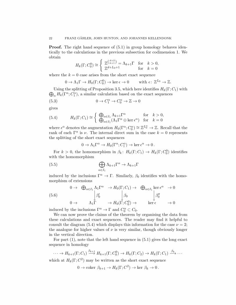
22 FRANZ GAHLER, JOHN HUNTON, AND JOHANNES KELLENDONK
Proof. The right hand sequence of (5.1) in group homology behaves iden-tically to the calculations in the previous subsection for codimension 1. Weobtain
Hk(Γ;C00 )
∼=
Z(d+2
k+1) = Λk+1Γ for k > 0,Zd+L0+1 for k = 0
where the k = 0 case arises from the short exact sequence
0 → Λ1Γ → H0(Γ;C00 ) → ker ǫ→ 0 with ǫ : ZL0 → Z.
Using the splitting of Proposition 3.5, which here identifiesHk(Γ;C1) with⊕
αHk(Γα;Cα1 ), a similar calculation based on the exact sequences
(5.3) 0 → Cα1 → Cα0 → Z → 0
gives
(5.4) Hk(Γ;C1) ∼=
⊕
α∈I1Λk+1Γ
α for k > 0,⊕
α∈I1(Λ1Γ
α ⊕ ker ǫα) for k = 0
where ǫα denotes the augmentation H0(Γα;Cα0 )
∼= ZLα0 → Z. Recall that the
rank of each Γα is ν. The internal direct sum in the case k = 0 representsthe splitting of the short exact sequences
0 → Λ1Γα → H0(Γ
α;Cα1 ) → ker ǫα → 0 .
For k > 0, the homomorphism in βk : Hk(Γ;C1) → Hk(Γ;C00 ) identifies
with the homomorphism
(5.5)⊕
α∈I1
Λk+1Γα → Λk+1Γ
induced by the inclusions Γα → Γ. Similarly, β0 identifies with the homo-morphism of extensions
(5.6)
0 →⊕
α∈I1Λ1Γ
α → H0(Γ;C1) →⊕
α∈I1ker ǫα → 0
y
β′0
y
β0
y
β′′0
0 → Λ1Γ → H0(Γ;C00 ) → ker ǫ → 0
induced by the inclusions Γα → Γ and Cα0 ⊂ C0.We can now prove the claims of the theorem by organising the data from
these calculations and exact sequences. The reader may find it helpful toconsult the diagram (5.4) which displays this information for the case ν = 2;the analogue for higher values of ν is very similar, though obviously longerin the vertical direction.
For part (1), note that the left hand sequence in (5.1) gives the long exactsequence in homology
· · · → Hk+1(Γ;C1)βk+1
−→ Hk+1(Γ;C00 ) → Hk(Γ;C2) → Hk(Γ;C1)
βk−→ · · ·
which at Hk(Γ;C2) may be written as the short exact sequence
0 → coker βk+1 → Hk(Γ;C2) → ker βk → 0 .

INTEGRAL COHOMOLOGY OF RATIONAL PROJECTION METHOD PATTERNS 23
This splits since ker βk ⊂ Hk(Γ;C1) is finitely generated free abelian.For part (2) it is sufficient to work with rational coefficients and count
ranks. Note that Rk is the rank of the image of βk and that β0 is surjective.For part (3), the torsion part of Hk(Γ;C2) must arise from coker βk+1
since ker βk is free. However, as the rank of Λk+2Γα is
(
νk+2
)
, for k > d/2 =ν− 1 this is trivial and so in this range the map βk+1 is zero and there is notorsion in its cokernel.
This final result, putting bounds on where torsion may appear, will be seento be a special case of a result for arbitrary codimension in Subsection 6.4.Examples suggest that these bounds are best possible.
A direct computation of ker β0 from the data encoded in ker β′0 and ker β′′0and the diagram (5.6) need not be immediate, a point which will becomea serious issue when we deal with the codimension 3 patterns later. Thediagram (5.6) gives a an exact sequence
0 → ker β′0 → ker β0 → ker β′′0∆0→ coker β′0 → 0
(coker β0 = 0 as β0 is surjective). In general there is no reason why the con-necting map ∆0 : ker β
′′0 → coker β′0 should be trivial. In fact, the Tubingen
Triangle Tiling [3, 32] tiling is an example in which coker β′0 = Z5 and hence∆0 is non-trivial. However, we do not need to compute ∆0 explicitly asthe coker β′0 term will only be comprised of torsion terms, which do notcontribute either to the torsion or the free rank of the cohomology of thetiling.

24 FRANZ GAHLER, JOHN HUNTON, AND JOHANNES KELLENDONK
Diagram 5.4. The entire computation for the case ν = 2, i.e., codimension= dimension = 2 can be summarized in the following diagram in which allrows and columns are exact.
0 =⊕
α∈I1Λ4Γ
α = H3(Γ;C1)
y
β3
Z = Λ4Γ = H3(Γ;C00 )
y
H2(Γ;C2) = H0(Ω)
y
0 =⊕
α∈I1Λ3Γ
α = H2(Γ;C1)
y
β2
Z4 = Λ3Γ = H2(Γ;C00 )
y
H1(Γ;C2) = H1(Ω)
y
ZL1 =⊕
α∈I1Λ2Γ
α = H1(Γ;C1)
y
β1
Z(2ν
2 ) = Λ2Γ = H1(Γ;C00 )
y
H0(Γ;C2) = H2(Ω)
y
0 →⊕
α∈I1Λ1Γ
α → H0(Γ;C1) →⊕
α∈I1ker ǫα → 0
y
β′0
y
β0
y
β′′0
0 → Λ1Γ → H0(Γ;C00 ) → ker ǫ → 0
y
0
5.3. Example computations. All examples discussed below have to someextent been calculated by computer. For this purpose, we have used thecomputer algebra system GAP [26], the GAP package Cryst [16, 17], as wellas further software written in the GAP language. It should be emphasizedthat these computations are not numerical, but use integers and rationals

INTEGRAL COHOMOLOGY OF RATIONAL PROJECTION METHOD PATTERNS 25
of unlimited size or precision. Neglecting the possibility of programmingerrors, they must be regarded as exact.
One piece of information that needs to be computed is the set of all in-tersections of singular affine subspaces, along with their incidence relations.This is done with code based on the Wyckoff position routines from theCryst package. The set of singular affine subspaces is invariant under theaction of a space group. Cryst contains routines to compute intersectionsof such affine subspaces and provides an action of space group elements onaffine subspaces, which allows to compute space group orbits. These rou-tines, or variants thereof, are used to determine the space group orbits ofrepresentatives of the singular affine subspaces, and to decompose them intotranslation orbits. The intersections of the affine subspaces from two trans-lation orbits is the union of finitely many translation orbits of other affinesubspaces. These intersections can be determined essentially by solving alinear system of equations modulo lattice vectors, or modulo integers whenworking in a suitable basis. With these routines, it is possible to generatefrom a space group and a finite set W of representative singular affine spacesthe set of all singular spaces, their intersections, and their incidences.
A further task is the computation of ranks, intersections, and quotientsof free Z-modules, and of homomorphisms between such modules, includingtheir kernels and cokernels. These are standard algorithmic problems, whichcan be reduced to the computation of Smith and Hermite normal forms ofinteger matrices, including the necessary unimodular transformations [13].GAP already provides such routines, which are extensively used.
The codimension 2 examples discussed here all have dihedral symmetryof order 2n, with n even. The lattice Γ⊥
n is given by the Z-span of thevectors in the star ei = (cos(2πi
n), sin(2πi
n)), i = 0, . . . , n − 1. The singular
lines have special orientations with respect to this lattice. They are parallelto mirror lines of the dihedral group, which means that they are eitheralong the basis vectors ei, or between two neighboring basis vectors, i.e.,along ei + ei+1. In all our examples below, with the single exception ofthe generalized Penrose tilings [36], one line from each translation orbitpasses through the origin. We denote the sets of representative singularlines by Wa
n and Wbn, for lines along and between the basis vectors ei. The
defining data of several well-known tilings can now be given as a pair of a(projected) lattice, and a set of translation orbit representatives of singularlines. Specifically, the Penrose tiling [15] is defined by the pair (Γ⊥
10,Wa10),
the Tubingen Triangle Tiling (TTT) [3, 32] by the pair (Γ⊥10,W
b10), the
undecorated octagonal Ammann-Beenker tiling [6] by the pair (Γ⊥8 ,W
a8 ), and
the undecorated Socolar tiling [41] by the pair (Γ⊥12,W
a12). For the decorated
versions of the Ammann-Beenker [41, 1, 22] and Socolar tilings [41], the set ofsingular lines Wa
n has to be replaced by Wan∪W
bn, n = 8 and 12, respectively.
These well-known examples are complemented by the coloured Ammann-Beenker tiling with data (Γ⊥
8 ,Wb8), which can be realised geometrically by

26 FRANZ GAHLER, JOHN HUNTON, AND JOHANNES KELLENDONK
Table 1. Cohomology of codimension 2 tilings with dihedral symmetry.
Tiling H2 H1 H0
Ammann-Beenker (undecorated) Z9 Z5 Z1
Ammann-Beenker (coloured) Z14 ⊕ Z2 Z5 Z1
Ammann-Beenker (decorated) Z23 Z8 Z1
Penrose Z8 Z5 Z1
generalized Penrose Z34 Z10 Z1
Tubingen Triangle Z24 ⊕ Z2
5Z5 Z1
Socolar (undecorated) Z28 Z7 Z1
Socolar (decorated) Z59 Z12 Z1
colouring the even and odd vertices of the classical Ammann-Beenker tilingwith two different colours, and the heptagonal tiling from [24], which is givenby the pair (Γ⊥
14,Wa14). Except for the coloured Ammann-Beenker tiling,
which had not been considered in the literature previously, the rationalranks of the cohomology of these tilings had been computed in [24]. Table 1shows their cohomology with integer coefficients, including the torsion partswhere present.
The generalized Penrose tilings [36] are somewhat different from the tilingsdiscussed above. They are built upon the decagonal lattice Γ⊥
10 too, but haveonly fivefold rotational symmetry. The singular lines do not pass throughthe origin in general, and their positions depend on a continuous parameterγ. For instance, the representative lines of the two translation orbits of linesparallel to e0 pass through the points −γe1 and γ(e1+e2). It turns out thatthese shifts of line positions always lead to the same line intersections andincidences. Even multiple intersection points remain stable, and are onlymoved around if γ is varied. Consequently, all generalized Penrose tilingshave the same cohomology, except for γ ∈ Z[τ ], which corresponds to thereal Penrose tilings [15]. This had already been observed by Kalugin [29],and is in contradiction with the results given in [24], which were obtaineddue to a wrong parametrisation of the singular line positions. Correctedresults are given in Table 1.
Among the tilings discussed above, only the TTT and the coloured Ammann-Beenker tiling have torsion in their cohomology. The set of singular lines ofthe TTT is constructed from the lines Wb
10. The translation stabilizers Γα
of all these lines are contained in a common sublattice Γ′⊥10 generated by the
star of vectors ei + ei+1; it has index 5 in Γ⊥10. It is therefore not too sur-
prising that coker β1 (Theorem 5.3) develops a torsion component Z25, which
shows up in the cohomology group H2 of the TTT, in agreement with theresults obtained using the method of Anderson-Putnam [2] which computesthe cohomology of TTT via its substitution structure. In much the same

INTEGRAL COHOMOLOGY OF RATIONAL PROJECTION METHOD PATTERNS 27
way, and for analogous reasons, a torsion component Z2 in H2 is obtainedalso for the coloured Ammann-Beenker tiling, and also the four-dimensional,codimension 2 tilings with data (Γ⊥
14,Wb14) have torsion components Z4
7 inH4, and Z3
7 in H3, in agreement with the bounds given in Theorem 5.3.There is an interesting relation between the TTT and the Penrose tiling.
Since the lattice Γ′⊥10 is rotated by π/10 with respect to Γ⊥
10, the TTT canalso be constructed from the pair (Γ′⊥
10 ,Wa10). However, the singular set
Γ′⊥10 + Wa
10 is even invariant under all translations from Γ⊥10, so that it is
equal to Γ⊥10 + Wa
10, which defines the Penrose tiling. In other words, theTTT and the Penrose tiling have the same set of singular lines, only thelattice Γ⊥ acting on it is different. The TTT is obtained by breaking thetranslation symmetry of the Penrose tiling to a sublattice of index 5. Thisexplains why the Penrose tiling is locally derivable from the TTT, but localderivability does not hold in the opposite direction [4]. A broken symmetrycan be restored in a local way, but the full lattice symmetry cannot bebroken to a sublattice in any local way, because there are no local means todistinguish the five cosets of the sublattice. Any tiling whose set of singularlines accidentally has a larger translation symmetry are likely candidates forhaving torsion in their cohomology.
For the coloured Ammann-Beenker tiling, the situation is completely anal-ogous. Geometrically, the coloured and the uncoloured version are the same,and thus have the same singular lines Wa
8 . For the coloured variant, we haveto restrict the lattice to the colour preserving translations, which form a sub-lattice Γ′⊥
8 of index 2 in Γ⊥8 . With respect to Γ′⊥
8 , the lines inWa8 are between
the generating vectors, so that the pair (Γ′⊥8 ,W
a8 ) is equivalent to the pair
(Γ⊥8 ,W
b8). Again, the uncoloured Ammann-Beenker tiling can be recovered
from the coloured one by restoring the translations broken by the colouring.
6. Patterns of codimension three
The case of projection patterns of codimension 3 is a good deal more com-plex than the codimension 2 theory, though the principles of computationremain the same. We shall initially consider almost canonical projectionpatterns with finitely generated cohomology (equivalently, that L0 is finite).Later we shall specialise to the rational projection patterns.
The dimension 3 space E⊥ now has families of singular lines and singularplanes. Following [21] we shall index by θ the lines and by α the planes.The rank of the main group Γ is N and, by Theorem 2.10, the rank of thestabiliser Γα of a singular plane is N − ν = 2ν, while the stabiliser Γθ of asingular line has rank ν.
The complex (3.2) in this case can be broken into two exact sequences
(6.1) 0 → C3 → C2 → C01 → 0 and 0 → C0
1 → C1 → C0 → Z → 0 .
The left hand sequence gives the long exact sequence
· · · → Hs(Γ;C3) → Hs(Γ;C2)φs−→ Hs(Γ;C
01 ) → Hs−1(Γ;C3) → · · ·

28 FRANZ GAHLER, JOHN HUNTON, AND JOHANNES KELLENDONK
computing H∗(Γ;C3) = Hd−∗(Ω) so long as we know the groups and homo-morphisms
φs : Hs(Γ;C2) → Hs(Γ;C01 )
and can solve the resulting extension problems. The groups Hs(Γ;C01 ) are
computed from the right hand sequence of (6.1) following exactly the sameprocedure we used to compute the codimension 2 examples from the analo-gous complex. We obtain
Lemma 6.1. There are equalities and short exact sequences
Hs(Γ;C01 ) = 0 for s > N − 1,
Hs(Γ;C01 ) = Λs+2Γ for N − 1 > s > ν,
0 → Λs+2Γ → Hs(Γ;C01 ) → ker γs → 0 , for ν > s > 1,
0 → coker γ1 → H0(Γ;C01 ) → ker γ0 → 0 ,
where, for s > 0,
γs : Hs(Γ;C1) =⊕
θ∈I1
Λs+1Γθ → Hs(Γ;C
00 ) = Λs+1Γ ,
and0 →
⊕
θ∈I1Λ1Γ
θ → H0(Γ;C1) →⊕
θ∈I1ker ǫθ → 0
y
γ′0
y
γ0
y
γ′′0
0 → Λ1Γ → H0(Γ;C00 ) → ker ǫ → 0
are both induced by the inclusions Γθ → Γ and Cθ0 ⊂ C0. Note that all theterms in (6.1) are free of torsion except possibly the coker γ1 summand.
By Proposition 3.5 the groups H∗(Γ;C2) split as⊕
α∈I2H∗(Γ
α;Cα2 ) andfor each singular plane Cα2 we have a sequence
0 → Cα2 → Cα1 → Cα0 → Z → 0 .
As before, we obtain
Lemma 6.2.
Hs(Γα;Cα2 ) = 0 for s > 2ν − 1,
Hs(Γα;Cα2 ) = Λs+2Γ
α for 2ν − 1 > s > ν,0 → Λs+2Γ
α → Hs(Γα;Cα2 ) → ker βαs → 0 , ν > s > 1
0 → coker βα1 → H0(Γα;Cα2 ) → ker βα0 → 0 ,
where, for s > 0,
βαs : Hs(Γ;Cα1 ) =
⊕
θ∈Iα1
Λs+1Γθ → Hs(Γ
α;Cα00 ) = Λs+1Γα ,
and
0 →⊕
θ∈Iα1Λ1Γ
θ → H0(Γ;Cα1 ) →
⊕
θ∈Iα1ker ǫθ → 0
y
βα0′
y
βα0
y
βα0′′
0 → Λ1Γα → H0(Γ;C
α00 ) → ker ǫα → 0.
INTEGRAL COHOMOLOGY OF RATIONAL PROJECTION METHOD PATTERNS 29
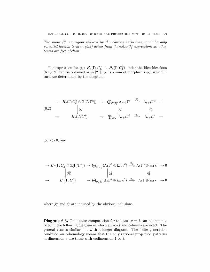
The maps βαs are again induced by the obvious inclusions, and the onlypotential torsion term in (6.2) arises from the coker βα1 expression; all otherterms are free abelian.
The expression for φs : Hs(Γ;C2) → Hs(Γ;C01 ) under the identifications
(6.1, 6.2) can be obtained as in [21]: φs is a sum of morphisms φαs , which inturn are determined by the diagrams
(6.2)
→ Hs(Γ;Cα2 ⊗ Z[Γ/Γα]) →
⊕
θ∈Iα1Λs+1Γ
θ βαs−→ Λs+1Γ
α →
y
φαs
y
jαs
y
ıαs
→ Hs(Γ;C01 ) →
⊕
θ∈I1Λs+1Γ
θ γs−→ Λs+1Γ →
for s > 0, and
→ H0(Γ;Cα2 ⊗ Z[Γ/Γα]) →
⊕
θ∈Iα1(Λ1Γ
θ ⊕ ker ǫθ)βα0−→ Λ1Γ
α ⊕ ker ǫα → 0
y
φα0
y
jα0
y
ıα0
→ H0(Γ;C01 ) →
⊕
θ∈I1(Λ1Γ
θ ⊕ ker ǫθ)γ0−→ Λ1Γ⊕ ker ǫ → 0
where jαs and ıαs are induced by the obvious inclusions.
Diagram 6.3. The entire computation for the case ν = 2 can be summa-rized in the following diagram in which all rows and columns are exact. Thegeneral case is similar but with a longer diagram. The finite generationcondition on cohomology means that the only rational projection patternsin dimension 3 are those with codimension 1 or 3.

30 FRANZ GAHLER, JOHN HUNTON, AND JOHANNES KELLENDONK
(6.3)
0 =⊕
α∈I2Λ6Γ
α = H4(Γ;C2)
y
Z = Λ6Γ = H4(Γ;C01 )
y
H3(Γ;C3) = H0(Ω) = Z
y
0 =⊕
α∈I2Λ5Γ
α = H3(Γ;C2)
y
Z6 = Λ5Γ = H3(Γ;C01 )
y
H2(Γ;C3) = H1(Ω)
y
0 →⊕
α∈I2Λ4Γ
α → H2(Γ;C2) → 0
y
φ′2
y
φ2
0 → Λ4Γ → H2(Γ;C01 ) → 0
y
H1(Γ;C3) = H2(Ω)
y
0 →⊕
α∈I2Λ3Γ
α → H1(Γ;C2) →⊕
α∈I2ker βα1 → 0
y
φ′1
y
φ1
y
φ′′1
0 → Λ3Γ → H1(Γ;C01 ) → ker γ1 → 0
y
H0(Γ;C3) = H3(Ω)
y
0 →⊕
α∈I2coker βα1 → H0(Γ;C2) →
⊕
α∈I2ker βα0 → 0
y
φ′0
y
φ0
y
φ′′0
0 → coker γ1 → H0(Γ;C01 ) → ker γ0 → 0
y
0

INTEGRAL COHOMOLOGY OF RATIONAL PROJECTION METHOD PATTERNS 31
As for the case n = 2 we shall compute first with rational coefficients andin so doing compute the ranks of the free abelian part of the integral coho-mology H∗(Ω), and second consider the torsion part. Although the rationalcomputation amounts to counting dimensions and using the extension
0 → coker φs+1 → Hs(Γ;C3) → kerφs → 0
the computation in terms of accessible numbers does not follow immediatelyby chasing Diagram 6.3 or its analogue for higher ν: for example, the rankof coker φs+1 is not automatically the sum of the ranks of coker φ′s+1 andcoker φ′′s+1, and likewise for the kernels. As before, a simple application ofthe snake lemma tells us that there are six term exact sequences
(6.4) 0→ker φ′s→kerφs→ker φ′′s∆s−→coker φ′s→coker φs→coker φ′′s→0.
As in the codimension 2 case, direct knowledge of ∆0 is unnecessary to solvefor either the rational ranks or the torsion. However, the maps ∆s, s > 0,enter into consideration in both cases; of course ∆s is trivial for s > ν sincekerφ′′s = 0 in these degrees.
The following lemma gives a useful link between the data required forcomputations using the set-up just described, based on the long exact se-quence (3.5), and the approach to computingH∗(Ω) which uses the sequence(3.9). Note that in the case of a rational projection pattern, j∗ is essentiallythe homomorphism α∗ of Corollary 4.10. It will give us a helpful criterionfor deciding when ∆s vanishes.
Lemma 6.4. For s > 0, the cokernel of j∗ : Hs+2(Γ;A∗⊗R) → Hs+2(Γ;T ∗⊗R) is identical to coker (φ′s)/im∆s. In particular, ∆s = 0 if and only ifcoker (j∗) = coker (φ′s).
Proof. By the exact sequence (3.9), coker (j∗) = im (m∗). As we can writem as the composite T ∗ → D2
∗ → D3∗ = C3[3] in M∗, we may identify the
composite
Λs+2Γ → Hs(Γ;C01 ) → Hs+2(Γ;C3[3]) = Hs−1(Γ;C3)
in Diagram 6.3 (or its analogue for higher values of ν) with m∗ in H∗(Γ;−).Thus im (m∗) = coker (j∗) can be identified with the image of the composite
coker (φ′s) → coker (φs) → Hs−1(Γ;C3)
which, by the exact sequence (6.4), is equal to coker (φ′s)/im∆s.
6.1. Rational computations. The computation of the rational ranks, i.e.,dimH∗(Γ;C3 ⊗Q), for an almost canonical projection pattern is now essen-tially straightforward, albeit longwinded. Clearly
dim Hs(Γ;C3 ⊗Q) = dim coker φs+1 + dim ker φs
and the computations follow from knowledge of the dimensions of the groupsH∗(Γ;C2 ⊗ Q) and H∗(Γ;C
01 ⊗ Q) obtained via the methods for n = 2,
together with a computation of the ranks of the maps φs. The latter are

32 FRANZ GAHLER, JOHN HUNTON, AND JOHANNES KELLENDONK
obtained relatively straightforwardly for s > ν, but for smaller values ofs the terms arising via φ′′s add a further degree of complexity and requireknowledge of ∆s. The following summarises the computation in the generalcase, and also corrects an error in the determination of the kernel of γ in[21] (middle of page 112). Applied to the Ammann-Kramer tiling [33], theseformulae evaluate to agree with the results of [29]. All of the terms usedin the statement can be calculated relatively easily on a computer provided∆s = 0, which we shall see below is the case for any rational projectiontiling when using rational coefficients.
Theorem 6.5. [Erratum1 to Theorem 2.7 of [21]] Given an almost canonicalprojection pattern with L0 finite, codimension 3 and dimension d = 3(ν −1), the following formulae give the ranks of the rational homology groupsH∗(Γ;C3 ⊗Q). All ranks are understood to be rational ranks. For s > 0,
rkHs(Γ;Cn ⊗Q) =
(
3ν
s+ 3
)
+ L2
(
2ν
s+ 2
)
+∑
α∈I2
Lα1
(
ν
s+ 1
)
+L1
(
ν
s+ 2
)
−Rs −Rs+1,
rkH0(Γ;Cn ⊗Q) =
3∑
j=0
(−1)j(
3ν
3− j
)
+ L2
2∑
j=0
(−1)j(
2ν
2− j
)
+∑
α∈I2
Lα1
1∑
j=0
(−1)j(
ν
1− j
)
+ L1
2∑
j=0
(−1)j(
ν
2− j
)
+e−R1 .
Here Rs = rkφs +∑
α∈I2rkβαs − rk γs + rk∆s which is given by, for s > 1
Rs = rk 〈Λs+2Γα : α ∈ I2〉+
∑
α∈I2
rk 〈Λs+1Γθ : θ ∈ Iα1 〉
−rk 〈Λs+1Γθ : θ ∈ I1〉+ rk∆s
and
R1 = rk 〈Λ3Γα/im βα : α ∈ I2〉+
∑
α∈I2
rk 〈Λ2Γθ : θ ∈ Iα1 〉
+rk 〈(⊕
θ∈Iα1
Λ2Γθ) ∩ ker γ1 : α ∈ I2〉 − rk 〈Λ2Γ
θ : θ ∈ I1〉+ rk∆1 .
Finally, the Euler characteristic e :=∑
s(−1)srkQHs(Γ;Cn) is given by
e = L0 −∑
α∈I2
Lα0 +∑
α∈I2
∑
θ∈Iα1
Lθ0 −∑
θ∈I1
Lθ0.
1The formulae given in [21] are correct only if the equation 〈im jαs ∩ ker γs : α ∈ I2〉 =ker γs in the middle of page 112 holds and rk∆s = 0. For the Ammann-Kramer tiling andthe dual canonical D6 tiling this is not so and the rank of the left hand side is one lowerthan that of the right.

INTEGRAL COHOMOLOGY OF RATIONAL PROJECTION METHOD PATTERNS 33
Remark 6.6. For s > ν the expression for Rs simplifies to Rs = rk 〈Λs+2Γα :
α ∈ I2〉. This follows from the fact that Λs+1Γθ vanishes for θ ∈ I1 or Iα1 as
the rank of Γθ is ν. For ν = 2, that is if the dimension is 3, the expressionfor R1 also simplifies slightly as imβα2 vanishes for similar reasons.
Now assume the projection pattern considered satisfies the rationality
conditions, and so we can use the geometric realisation Aα
−→ T of the
homomorphism A∗j
−→ T ∗ as in Theorem 4.9. In particular, Lemma 6.4tells us that ∆s = 0 if im (α∗) = im (φ′s).
Lemma 6.7. For a rational projection pattern, in computations of cohomol-ogy with any coefficient ring R a field of characteristic 0, the homomorphisms∆s = 0 for all s > 0.
Proof. Recall that A is given as a union of (N − ν)-tori Ti inside T. The
individual inclusions Ti → T combine to give a map factoring∐
Ti → Aα
−→T which shows that we always have the inclusion im (φ′s) ⊂ im (α∗); we provethe opposite inclusion. It is sufficient to work with the field F = R.
Consider a simplicial decomposition of the pair (T,A), that is, a simplicialdecomposition of T such that each (open) cell has either empty intersectionwith A or is contained in it. The map on simplicial chain groups givenby mapping the simplex (x0, . . . , xr) to (x1 − x0) ∧ · · · ∧ (xr − x0) ∈ ΛrRΓvanishes on boundaries and hence induces an isomorphism between Hr(T;R)and ΛrΓ⊗ R. Restricting to A = ∪Ti it follows that im (α∗) is contained inthe subgroup of ΛrΓ⊗R generated by the subgroups ΛrΓ
Di ⊗ R.
Corollary 6.8. For rational projection tilings rk∆s = 0 for all s > 0 andthe formulae in the statement of Theorem 6.5 correspondingly simplify.
6.2. Torsion and the integral computations. We turn to the determi-nation of the integral cohomology of almost canonical projection patternsand, given the results above for calculations with rational coefficients, thisentails an examination of the torsion groups which can arise in the compu-tations, and the solution of associated extension problems. As before, weassume throughout this subsection that the number L0 is finite, but do notas yet assume the rationality conditions.
The results of Lemmas 6.1 and 6.2 show that computations for Hs(Γ;C3)are relatively straightforward for s > ν; in these cases we have an extension
0 → coker(
φ′s+1 :⊕
α∈I2Λs+3Γ
α → Λs+3Γ)
→ Hs(Γ;C3)→ ker
(
(φ′s :⊕
α∈I2Λs+2Γ
α → Λs+2Γ)
→ 0
and this extension splits since the kernel term is free abelian. In fact asthe rank of Γα is 2ν we immediately recover the result of Corollary 4.12 forcodimension 3 patterns. As the cokernel term can in principle have torsion,this same observation about the rank of Γα gives the following analogueof the final line in Theorem 5.3; again examples suggest this result is bestpossible.
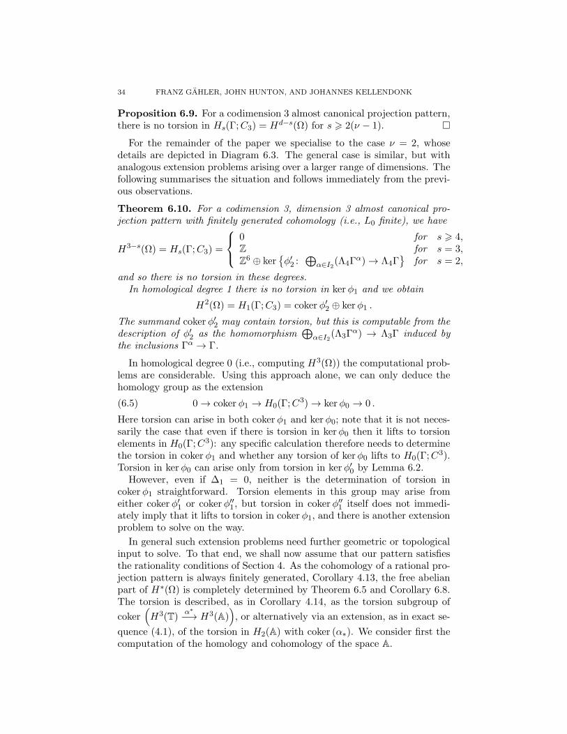
34 FRANZ GAHLER, JOHN HUNTON, AND JOHANNES KELLENDONK
Proposition 6.9. For a codimension 3 almost canonical projection pattern,there is no torsion in Hs(Γ;C3) = Hd−s(Ω) for s > 2(ν − 1).
For the remainder of the paper we specialise to the case ν = 2, whosedetails are depicted in Diagram 6.3. The general case is similar, but withanalogous extension problems arising over a larger range of dimensions. Thefollowing summarises the situation and follows immediately from the previ-ous observations.
Theorem 6.10. For a codimension 3, dimension 3 almost canonical pro-jection pattern with finitely generated cohomology (i.e., L0 finite), we have
H3−s(Ω) = Hs(Γ;C3) =
0 for s > 4,Z for s = 3,Z6 ⊕ ker
φ′2 :⊕
α∈I2(Λ4Γ
α) → Λ4Γ
for s = 2,
and so there is no torsion in these degrees.In homological degree 1 there is no torsion in ker φ1 and we obtain
H2(Ω) = H1(Γ;C3) = coker φ′2 ⊕ kerφ1 .
The summand coker φ′2 may contain torsion, but this is computable from thedescription of φ′2 as the homomorphism
⊕
α∈I2(Λ3Γ
α) → Λ3Γ induced bythe inclusions Γα → Γ.
In homological degree 0 (i.e., computing H3(Ω)) the computational prob-lems are considerable. Using this approach alone, we can only deduce thehomology group as the extension
(6.5) 0 → coker φ1 → H0(Γ;C3) → ker φ0 → 0 .
Here torsion can arise in both coker φ1 and ker φ0; note that it is not neces-sarily the case that even if there is torsion in kerφ0 then it lifts to torsionelements in H0(Γ;C
3): any specific calculation therefore needs to determinethe torsion in coker φ1 and whether any torsion of kerφ0 lifts to H0(Γ;C
3).Torsion in ker φ0 can arise only from torsion in ker φ′0 by Lemma 6.2.
However, even if ∆1 = 0, neither is the determination of torsion incoker φ1 straightforward. Torsion elements in this group may arise fromeither coker φ′1 or coker φ′′1 , but torsion in coker φ′′1 itself does not immedi-ately imply that it lifts to torsion in coker φ1, and there is another extensionproblem to solve on the way.
In general such extension problems need further geometric or topologicalinput to solve. To that end, we shall now assume that our pattern satisfiesthe rationality conditions of Section 4. As the cohomology of a rational pro-jection pattern is always finitely generated, Corollary 4.13, the free abelianpart of H∗(Ω) is completely determined by Theorem 6.5 and Corollary 6.8.The torsion is described, as in Corollary 4.14, as the torsion subgroup of
coker(
H3(T)α∗
−→ H3(A))
, or alternatively via an extension, as in exact se-
quence (4.1), of the torsion in H2(A) with coker (α∗). We consider first thecomputation of the homology and cohomology of the space A.

INTEGRAL COHOMOLOGY OF RATIONAL PROJECTION METHOD PATTERNS 35
⊕
α∈I2Λ4Γ
α
⊕
α∈I2Λ3Γ
α
⊕
α∈I2Λ2Γ
α ⊕⊕
θ∈I1Λ2Γ
θ⊕
α∈I2
⊕
θ∈Iα1Λ2Γ
θ
⊕
α∈I2Λ1Γ
α ⊕⊕
θ∈I1Λ1Γ
θ⊕
α∈I2
⊕
θ∈Iα1Λ1Γ
θ
ZL2 ⊕ ZL1 ⊕ ZL0⊕
α∈I2ZL
α1 ⊕
⊕
α∈I2ZL
α0 ⊕
⊕
θ∈I1ZL
θ0
⊕
α∈I2
⊕
θ∈Iα1ZL
θ0
Table 2. First page of the Mayer-Vietoris spectral sequencefor the homology of A.
We start with the homology of A. For elementary reasons, H0(A) = Z
and H1(A) = H1(T) = Z6. To compute the higher homology groups weuse the Mayer-Vietoris spectral sequence for the homology of the resolutionspace A∆. This considers A as the union of L2 4-tori, L1 2-tori and L0
0-tori (points). The E1-page of the spectral sequence has, as its rth columnE1r,∗, the homology of the disjoint union of those tori arising as (r + 1)-fold
intersections, as shown in Table 2.Knowledge of Hs(A) for r = 0 and 1 allows computation of the differ-
entials, and the only torsion that can arise is that in the cokernel of thedifferential d11,2 : E
11,2 → E1
0,2. This differential runs
d11,2 :⊕
α∈I2
(
⊕θ∈Iα1Λ2Γ
θ)
→ (⊕α∈I2Λ2Γ
α) ⊕ (⊕θ∈I1Λ2Γ
θ)
and is described explicitly on each component Λ2Γθ for θ ∈ Iα1 via the
canonical embeddings of the stabiliser subgroups Γθ into the correspondingΓα and Γθ in the target components. We obtain
Lemma 6.11. For a rational projection pattern with ν = 2, the only torsionwhich arise in H∗(A) is in H2(A) and is that which arises in the cokernelof the differential d11,2.
The cohomology calculations are formally dual to the above; note nowthat the important differential for torsion purposes runs d1,21 : E0,2
1 → E1,21 ,
giving potential torsion in its cokernel, the group E1,22 , that is, in cohomo-
logical dimension 3. This corresponds, via the universal coefficient theorem,to the identification of the torsion in H2(A) with that in H3(A).
In all the icosahedral tilings we consider below, this torsion group is non-trivial. For larger values of ν the corresponding Mayer-Vietoris spectralsequences are similar, though have more rows. Again, torsion can only arisefrom the cokernel of differentials d11,s where now 2 6 s 6 ν, and formulaefor these differentials are given by the analogues of the description for ν = 2above.

36 FRANZ GAHLER, JOHN HUNTON, AND JOHANNES KELLENDONK
Finally we note the following useful observation concerning a criterion forthe absence of torsion in the group coker (α∗). We state it for general valuesof ν.
Lemma 6.12. For a codimension 3 rational projection pattern and s > 0,if coker φ′s is torsion free then ∆s = 0 and hence coker (α∗) is torsion free.
Proof. By Lemma 6.7 we know that ∆s = 0 when working over R, andhence when working over Z the image of ∆s can only be a torsion group.If coker φ′s is torsion free then ∆s = 0 integrally. The result concerningcoker (α∗) now follows from Lemma 6.4
6.3. Codimension 3 examples with icosahedral symmetry. We illus-trate the above tools by considering the computations of the cohomologyof the four icosahedral tilings, the Danzer tiling [14], the Ammann-Kramertiling [33], the canonical D6 tiling [34] and the dual canonical D6 tiling [34],all of which are rational projection patterns. Preliminary results were an-nounced in [25], but, as we note below, at least in the case of the Danzertiling, the torsion component of the integral cohomology group H3(Ω) wasincorrectly computed there, as possibly were also the corresponding com-putations of H3 for the other three examples; the lower cohomology groupsannounced in [25] are correct. In this section we give details of these compu-tations. These examples also give a good overview of some of the differentphenomena that can occur in the determination of torsion.
We start by describing the relevant lattices Γ and families of singularplanes W. In three dimensions, there are three inequivalent icosahedrallattices of minimal rank 6.
The primitive lattice ΓP is generated by a star of vectors pointing fromthe center to the vertices of a regular icosahedron. We choose any basise1, . . . , e6 from this vector star. The lattice ΓF is then the sublattice ofthose integer linear combinations of the ei, whose coefficients add up to aneven integer. The lattice ΓI is given by the Z-span of the vectors in ΓP ,and the additional vector 1
2(e1 + . . . + e6). These lattices are analogues of
the primitive, F-centered, and I-centered cubic lattices.2 ΓF is an index-2sublattice of ΓP , which in turn is an index-2 sublattice of ΓI . The actionof the icosahedral group A5 on the three lattices gives rise to three integralrepresentations, which are inequivalent under conjugation in GL6(Z).
The singular planes of all four examples have special orientations, beingperpendicular either to a 5-fold, a 3-fold, or a 2-fold axis of the icosahedron(the latter are also parallel to a mirror plane). Moreover, each Γ-orbit ofsingular planes contains a representative which passes through the origin.We therefore define the families of planes Wn, n = 5, 3, 2, consisting of allplanes perpendicular to an n-fold axis, and passing through the origin. Thearrangements of singular planes of the icosahedral examples are then givenby the pair (ΓP ,W
2) for the Ammann-Kramer tiling, the pair (ΓF ,W2) for
2strictly speaking, 1
2ΓF is a centering of ΓP

INTEGRAL COHOMOLOGY OF RATIONAL PROJECTION METHOD PATTERNS 37
the dual canonical D6 tiling, the pair (ΓF ,W5) for the the Danzer tiling,
and the pair (ΓF ,W5 ∪ W3) for the canonical D6 tiling. Interestingly, the
sets ΓP +W2 and ΓF +W2 are invariant even under all translations fromΓI , which means that they are both equal to ΓI +W2. In other words, thesets of singular planes of the Ammann-Kramer tiling and the dual canonicalD6 tiling are the same, only the lattices acting on it by translation aredifferent. On the other hand, the sets of singular planes of the Danzer tilingand the canonical D6 tiling have a lattice of translation symmetries whichis equal to the lattice ΓF they are constructed from. With these data is itnow straightforward to evaluate the formulæ of Theorem 6.5 for the ranksof the rational homology groups. The results are summarized in Table 3. Ascan be seen, compared to previously published results the rational ranks ofH0 and H1 of the Ammann-Kramer tiling and the dual canonical D6 tilinghave been increased by 1, in agreement with Kalugin [29], whereas all otherrational ranks remain the same.
Next, we discuss the determination of torsion, which is potentially non-trivial only for H2 and H3, as noted by Proposition 6.9. The torsion in H2
is relatively straightforward, and can be computed, as in Theorem 6.10, asthe torsion in the cokernel of
φ2 : ⊕α∈I2 Λ4Γα → Λ4Γ .
Both the Ammann-Kramer and dual canonical D6 tilings have 2-torsion inH2(Ω) arising from this map; coker φ′2 is torsion free for the Danzer andcanonical D6 tilings, making their H2 groups free abelian.
This situation concerning the groups H3 is as follows. In each of thefirst three tilings coker φ′1 is torsion free and so by Lemma 6.12 the map∆1 is zero. This is not so for the dual canonical D6 tiling where additionalgeometric computation (such as that described in [25]) is needed to deducethat nevertheless coker (α∗) is still free. By Lemma 6.4, this implies thatthe map ∆1 is non-trivial, having image the whole of the torsion subgroupZ62 of coker φ′1.In every case there are 2-torsion components in coker φ′′1. For the first
three examples there is no other torsion arising in the computation via Di-agram (6.3), but there remains an extension problem of the form
0 → free abelian group → coker φ1 → coker φ′′1 → 0
which has more than one potential solution.For the dual canonical D6 tiling, the situation is more complicated. There
is torsion, Z72, in coker φ′′1, and an extension problem to decide its lift to
coker φ1, but there is also torsion, Z152 , in ker φ0, arising as the torsion in
kerφ′0. Then H3 is given by a further extension (6.5) running
(6.6) 0 → coker φ1 → H3(Ω) → Z328 ⊕ Z152 → 0 .
There is no direct way of solving such extension problems without someadditional geometric input, for example via the geometric realisation of the

38 FRANZ GAHLER, JOHN HUNTON, AND JOHANNES KELLENDONK
H3 ⊗Q H2 H1 H0 t′1 t′′1 t′0
Danzer Q20 Z16 Z7 Z 0 Z2 0
Ammann-Kramer Q181 Z72 ⊕ Z2 Z12 Z 0 Z2 0
canonical D6 Q205 Z72 Z7 Z 0 Z22 0
dual canonical D6 Q331 Z102 ⊕ Z42 ⊕ Z4 Z12 Z Z6
2 Z72 Z15
2
Table 3. [25] Integral cohomology H2, H1 and H0, andrational H3 of icosahedral tilings from the literature. Alsoindicated are details of the torsion arising at various pointsin the calculation via diagram (6.3). We use the notationthat t′1, t
′′1 and t′0 denote the torsion components of coker φ′1,
coker φ′′1 and kerφ′0 respectively.
rational projection pattern and computation of the corresponding torus ar-rangement A. Using the Mayer-Vietoris computation of H∗(A), it can beshown that, for this example, at least one of these extension is non-trivial.
Clearly each example at this point must be handled on a case by case basis.The Danzer tiling, arguably the simplest of these four, involves sufficientlysmall cell complexes that a complete solution is available. Computationsusing either Diagram (6.3) or the exact sequence (4.10) yield an extensionproblem for H3 with a single Z2 in the quotient: there is a simple dichotomy,that H3 is either Z20 ⊕ Z2 (the trivial extension), or is Z20 (the non-trivialone). However, for this tiling, a modified version of the Anderson-Putnamcomplex gives H3(Ω) as the direct limit of the cohomology H3(K) of acertain cell complex under an iterated self map f : K → K. Machine com-putation shows that there is no torsion in H3(K), and consequently therecan be none in the direct limit H3(Ω) = lim→H3(K). This determines theextension problem: it is the non-trivial one.
Corollary 6.13. The integral cohomology of the Danzer tiling is given by
H0(Ω) = Z H1(Ω) = Z7 H2(Ω) = Z16 H3(Ω) = Z20 .
6.4. K-theory and general codimension. We conclude with some re-marks on the general codimension case and the consequences of our workfor the K-theory of cut & project patterns. The first observation is anextension of the result of Corollary 4.12.
Proposition 6.14. For a general dimension d, codimension n, rational pro-jection tiling, the groups Hs(Ω) are free abelian of rank
(
Ns
)
if s < ν − 1,but the possibility of torsion exists for all s > ν − 1. For these values of s

INTEGRAL COHOMOLOGY OF RATIONAL PROJECTION METHOD PATTERNS 39
the torsion subgroup contains the torsion part of
coker
⊕
α
ΛN−sΓα α∗−→ ΛN−sΓ
and if s < 2ν − 1 then this is precisely the torsion term.
Sketch of Proof. By Corollary 4.10 we have an exact sequence
· · · → HN−s(A)α∗−→ HN−s(T) −→ Hs(Ω) −→ HN−s−1(A) → · · · .
If s < ν − 1, then N − s − 1 > (n − 1)ν and HN−s−1(A) = 0 since A isconstructed as the union of (n− 1)ν-dimensional tori. This proves the firstpart of the statement, a restatement of Corollary 4.12. The exact sequencealso shows that the cokernel term in the statement clearly injects in Hs(Ω),which forms the second part, and the final observation follows from a moredetailed computation of H∗(A). In brief, in the range s < 2ν−1, the groupsHN−s−1(A) are free abelian; this follows from a Mayer-Vietoris spectralsequence computation of H∗(A) as in [29], and uses the observation that thehighest homological dimension of intersection of the component (n−1)ν-torimaking up A is of dimension (n− 2)ν.
Examples lead us to conjecture that where this proposition indicates thatthere might be torsion, examples can be found where there is torsion.
We turn to consider the various forms of K-theory used in the study ofaperiodic tilings. Initial interest was in the K-theory of various noncommu-tative C∗-algebras associated to the tilings [7]. At the level of graded abeliangroups, the values of this K-theory is (modulo regrading) the same as thetopological K-theory of the tiling space, which we denote K∗(Ω) [18]. TheAtiyah-Hirzebruch spectral sequence (AHSS) provides a way of computingthe K-theory of Ω from its cohomology, and in the absence of torsion inH∗(Ω) it is a standard fact that this spectral sequence collapses and the K-theory is just the direct sum of the cohomology groups, K0(Ω) = ⊕sH
2s(Ω)and K1(Ω) = ⊕sH
2s−1(Ω). This is not necessarily so in the presence of tor-sion. However, for small values of d the situation remains straightforward.Standard topological arguments with the AHSS, using characterisation ofthe possible differentials yield
Proposition 6.15. For a dimension d 6 3 rational projection pattern,K0(Ω) = ⊕sH
2s(Ω) and K1(Ω) = ⊕sH2s−1(Ω).
Sketch of Proof. The smallest possible non-zero differential that can leadto the failure of this result is d3 : H
s(Ω) → Hs+3(Ω) and there must be 2-torsion in Hs+3(Ω). However, as H0(Ω) = Z and represents the connectivityelement, d3 can be non-trivial only for positive values of s; as we need anon-trival value of Hs+3(Ω) for d3 6= 0, we need the cohomology of Ω to benon-zero in some dimensions at least 4. This cannot happen if the tiling isonly 3 dimensional.

40 FRANZ GAHLER, JOHN HUNTON, AND JOHANNES KELLENDONK
As we know that ν must be an integer, the codimension of the pattern is3 or less, and torsion can only exist in cohomological dimensions 2 or 3; thisis enough to be sure that there are no extension problems and the K-theorysplits as the direct sum as claimed.
The possibility nevertheless exists for tilings in higher dimensions demon-strating significant differences between their cohomology and K-theory.
7. Appendix: realisation of H∗(Ω) as group (co)homology
We sketch briefly here the argument that H∗(Ω) can be realised as thegroup cohomology H∗(Γ;Cn) as noted at the start of Section 3. Thisidentification lies at the heart of the approach of [20, 21] and we directthe reader to [21] in particular for full details. It also enables us to jus-tify the identification of the homomorphisms µ∗ : H∗(T) → H∗(Ω) andm∗ : H
∗(Γ;T ∗) → H∗(Γ;Cn[n]) as mentioned in Remark 4.11.We recall from Section 2 that Ω can be considered as the completion
of q(NS) ⊂ T, the image of the non-singular points in the N -torus, withrespect to the pattern metric.
The translation action of E‖ on E passes to an action on T = E/Γ.Moreover, this action preserves S and NS and the resulting action on q(NS)is continuous in the pattern metric. Thus the dynamical system (q(NS), E‖)
extends to the completion yielding the dynamical system (Ω, E‖). Since
(q(NS), E‖) is a sub-system of a flow on the torus T, the system (Ω, E‖) isthe flow on the mapping torus of a Zd action.
To make this explicit, choose a splitting Γ = Γ1⊕Γ2 where Γ1 is of rank n,and Γ2 is of rank d. Then Γ1 spans a linear space F ⊂ E and we can pick afundamental domain X ⊂ F . Let Xc be the completion of q(X ∩NS) in thepattern metric and Fc the corresponding completion of q(F ∩NS). Then Ω isthe mapping torus of the action of Γ2
∼= Zd on Xc given on q(x) ∈ q(X∩NS)
by γ · q(x) = q(x− πF (γ)), where πF is the projection onto F along E‖.Identifying Ω with this mapping torus, it follows that the Cech coho-
mology of Ω can be identified with H∗(Γ2;C(Xc,Z)) the group cohomologyof Γ2 with values in the representation module C(Xc,Z), the continuousZ-valued functions on Xc, defined by this action. This can be seen, forexample, by viewing the mapping torus as a fibre bundle over the d-torusBΓ2 with fibre Xc: then the Serre spectral sequence of the bundle hasE2 = E∞-term H∗(Γ2;H
∗(Xc)), and the Cech cohomology H∗(Xc) of thetotally disconnected space Xc is precisely C(Xc,Z). Moreover, as Γ1 actsfreely on C(Fc,Z) by the analogous action, we can identify H∗(Γ2;C(Xc,Z))with H∗(Γ;C(Fc,Z)). Finally, the assumption of total irrational position al-lows us to identify C(Fc,Z) with C(E⊥
c ,Z)), as Γ-modules, where E⊥c is the
completion of E⊥ ∩NS in the pattern metric, as in Section 3. Summing up,we have the string of identifications
H∗(Ω) ∼= H∗(Γ2;C(Xc,Z)) ∼= H∗(Γ;C(Fc,Z)) ∼= H∗(Γ;C(E⊥c ,Z)) .

INTEGRAL COHOMOLOGY OF RATIONAL PROJECTION METHOD PATTERNS 41
As noted after Definition 3.1, we may identify C(E⊥c ,Z)) with the Γ-module
Cn. The equivalence Hs(Γ;Cn) ∼= Hd−s(Γ;Cn) in (3.1) follows from thePoincare duality property of the group Γ2.
We turn to the map µ : Ω → T. The identifications above allow us to viewΩ cohomologically as the fibre bundle over BΓ with fibre E⊥
c ; in the sameway, we can replace the space T by the bundle over BΓ with fibre E⊥ andthe homomorphism µ∗ is represented in cohomology by H∗(Γ;C(E⊥;Z)) →H∗(Γ;C(E⊥
c ;Z)) induced by the natural quotient E⊥c → E⊥. By the analo-
gous argument along the lines of the proof of Theorem 4.9, this is the samemap in cohomology as induced in H∗(Γ;−) by the map T ∗ → Cn[n].
References
[1] R. Ammann, B. Grunbaum, and G.C. Shephard, Aperiodic Tiles, Discrete Comput.
Geom. 8 (1992) 1–25.[2] J.E. Anderson and I.F. Putnam, Topological invariants for substitution tilings and
their associated C∗-algebras, Ergod. Th. & Dynam. Syst. 18 (1998) 509–537.[3] M. Baake, P. Kramer, M. Schlottmann, and D. Zeidler, Planar patterns with fivefold
symmetry as sections of periodic structure in 4-space, Int. J. Mod. Phys. B 4 (1990)2217–2268.
[4] M. Baake, M. Schlottmann and P.D. Jarvis, Quasiperiodic tilings with tenfold sym-metry and equivalence with respect to local derivability, J. Phys. A: Math. Gen. 24(1991) 4637–4654.
[5] M. Barge, H. Bruin, L. Jones and L. Sadun, Homological Pisot substitutions andexact regularity, math.DS 1001.2027.
[6] F.P.M. Beenker, Eindhoven University of Technology Report 82-WSK-04 (1982).[7] J. Bellissard, K-theory of C∗-algebras in solid state physics, Statistical Mechanics
and Field Theory: Mathematical aspects, ed. T. C. Dorlas, Springer Berlin (1986)99-156.
[8] J. Bellissard, R. Benedetti, J-M. Gambaudo, Spaces of tilings, finite telescopic ap-proximations and gap-labeling, Communications in Mathematical Physics, 261 (2006)1-41.
[9] J. Bellissard, D. Hermmann and M. Zarrouati, Hull of aperiodic solids and gap label-ing theorems, in Directions in Mathematical Quasicrystals, CRM Monograph Series,Volume 13, M.B. Baake and R.V. Moody, eds., Providence, RI: AMS 2000, pp. 207-259.
[10] J. Bellissard, J. Kellendonk, and A. Legrand, Gap-labelling for three dimensionalaperiodic solids. C. R. Acad. Sci. Paris, t.332, Serie I (2001) 1–5.
[11] M-T. Benameur, H. Oyono-Oyono, Index theory for quasi-crystals. I. Computationof the gap-label group. (English summary) J. Funct. Anal. 252 (2007), no. 1, 137170.
[12] A. Clark and L. Sadun, When shape matters: deformations of tiling spaces, ErgodicTheory and Dynamical Systems 26 (2006) 69-86.
[13] H. Cohen, A course in computational algebraic number theory, 2nd edition, Springer,Berlin, Heidelberg 1995.
[14] L. Danzer, Three dimensional analogues of the planar Penrose tilings and quasicrys-tals, Discrete Math. 76 (1989) 1-7.
[15] N.G. de Bruijn, Algebraic theory of Penrose’s aperiodic tilings of the plane, Math.
Proc. A84 (1981) 39-66.[16] B. Eick, F. Gahler and W. Nickel, Computing Maximal Subgroups and Wyckoff
Positions of Space Groups, Acta Cryst. A53 (1997) 467–474.

42 FRANZ GAHLER, JOHN HUNTON, AND JOHANNES KELLENDONK
[17] B. Eick, F. Gahler, and W. Nickel, Cryst – Com-puting with crystallographic groups, Version 4.1.6 (2008)(\protect\vrule width0pt\protect\hrefhttp://www.gap-system.org/Packages/cryst.htmlhttp://www.gap-system.org/Packages/cryst.html)
[18] A.H. Forrest and J.R. Hunton, The cohomology and K-theory of commuting homeo-morphisms of the Cantor set, Ergod. Th. and Dynam. Sys., 19 (1999) 611-625.
[19] A.H. Forrest, J.R. Hunton and J. Kellendonk, Topological invariants for projectionmethod patterns, Proc Int. Congress. Math. Phys. London 2000.
[20] A.H. Forrest, J.R. Hunton and J. Kellendonk, Cohomology of canonical projectiontilings, Comm. Math. Phys. 226 (2002) 289-322.
[21] A.H. Forrest, J.R. Hunton and J. Kellendonk, Topological invariants for projectionmethod patterns, Mem. Amer. Math. Soc. 758 (2002).
[22] G. Gahler, Matching Rules for Quasicrystals: The Composition-DecompositionMethod, J. Non-Cryst. Solids 153 & 154 (1993) 160–164.
[23] F. Gahler, Lectures and unpublished notes on torsion in the homology of the TubingenTriangle Tiling, Banff and elsewhere. (2004).
[24] F. Gahler and J. Kellendonk, Cohomology groups for projection tilings of codimension2, Materials Science and Engineering. 438-440 (2000) 294-296.
[25] F. Gahler, J.R. Hunton and J. Kellendonk, Integer Cech cohomology of icosahedralprojection tilings, Z. Kristallogr. 223 (2008) 801-804.
[26] The GAP Group GAP – Groups, Algorithms, and Programming, Version 4.4.12(2008) (\protect\vrule width0pt\protect\hrefhttp://www.gap-system.orghttp://www.gap-system.org).
[27] C. Irving, Euler characteristics and cohomology for quasiperiodic projection patterns,PhD thesis, University of Leicester, 2006.
[28] A. Julien, Complexity and cohomology for cut-and-projection tilings, Ergodic Theory
and Dynamical Systems, 30 (2010) 489-523.[29] P. Kalugin. Cohomology of quasiperiodic patterns and matching rules, J. Phys. A:
Math. Gen. 38 (2005) 3115–3132.[30] J. Kaminker and I. Putnam, A proof of the gap labelling conjecture, Mich. Math. J.,
51 (2003) 537-546.[31] J. Kellendonk, Pattern equivariant functions, deformations and equivalence of tiling
spaces, Ergodic Theory and Dynamical Systems 28 (2008) 1153-1176.[32] R. Klitzing, M. Schlottmann, and M. Baake, Perfect matching rules for undecorated
triangular tilings with 10-, 12-, and 8-fold symmtery, Int. J. Mod. Phys. B 7 (1993)1455–1473.
[33] P. Kramer and R. Neri, On periodic and non-periodic space fillings of Em obtainedby projection, Acta Cryst A 40 (1984) 580–587.
[34] P. Kramer and Z. Papadopolos, Models of icosahedral quasicrystals from 6d lattices,Proceedings of the International conference on Aperiodic Crystals, Aperiodic ’94(G. Chapuis et al., ed.), World Scientific, Singapore, 1995, pp. 70–76.
[35] R. Moody. Model sets: A Survey, From Quasicrystals to More Complex Systems, eds.F. Axel, F. Dnoyer, J.P. Gazeau, Centre de physique Les Houches, Springer Verlag,2000.
[36] A. Pavlovitch and M. Kleman, Generalised 2D Penrose tilings: structural properties,J. Phys. A: Math. Gen. 20 (1987) 687–702.
[37] I. Putnam. Non-commutative methods for the K-theory of C*-algebras of aperiodicpatterns from cut-and-project systems. Comm. Math. Phys., 294(2010), 703-729.
[38] L. Sadun and R.F. Williams, Tiling spaces are Cantor set bundles, Ergodic Theory
and Dynamical Systems, 23 (2003), 307–316.[39] L. Sadun, Topology of Tiling Spaces, University Lecture Series, AMS vol.46, (2008).[40] L. Sadun, Exact regularity and the cohomology of tiling spaces, math.DS 1004.2281.[41] J.E.S. Socolar. Simple octagonal and dodecagonal quasicrystals, Phys. Rev. B 39
(1989) 10519–10551.

INTEGRAL COHOMOLOGY OF RATIONAL PROJECTION METHOD PATTERNS 43
[42] W. Steurer and S. Deloudi, Crystallography of Quasicrystals, Springer Series in Ma-
terials Science 126, Springer 2009.[43] C. Wiebel. An introduction to homological algebra, Cambridge studies in advanced
mathematics 38 (1994), CUP.
Faculty of Mathematics, University of Bielefeld, D-33615 Bielefeld, Ger-many.
E-mail address: [email protected]
The Department of Mathematics, University of Leicester, Leicester, LE17RH, England.
E-mail address: [email protected]
Universite de Lyon, Universite Claude Bernard Lyon 1, Institut CamilleJordan, CNRS UMR 5208, 43 boulevard du 11 novembre 1918, F-69622 Villeur-banne cedex, France.
E-mail address: [email protected]