Integer Programming Model for Inventory … Programming Model for Inventory Optimization for a Multi Echelon System . ... A supply chain network ... simulation models and abstract

Integer Programming Model for Inventory

Optimization for a Multi Echelon System

Bassem H. Roushdy Basic and Applied Science, Arab Academy for Science and Technology, Cairo, Egypt

Email: [email protected]

Abstract—The interest in supply chain management and its

optimization as complex systems is rapidly growing. In this

research, the interaction among different entities in the

supply chain is considered where a repeated process of

orders and production occur. A supply chain network

consisting of multi-echelon manufacturing center and one

demand center is considered. A mixed integer programming

model is developed to determine production and inventory

decisions across different entities supply chain. The

objective here is to determine warehouse allocation places in

the supply chain to have minimum inventory cost of the

system.

Index Terms—supply chains, integer programming,

inventory coordination & optimization

I. INTRODUCTION

Inventory optimization remains one of the key

challenges in supply chain management. Typically, large

amounts of working capital are tied up in today’s supply

chains, restricting the opportunities for growth that are

essential for a company’s success in competitive markets.

However, researches have shown that inventories have a

high opportunity to reduce them within supply chain, and

hence increasing competiveness factors and reduce

production costs.

A supply chain may be defined as an integrated

process wherein a number of various business entities

like suppliers, manufacturers, distributors, and retailers

work together in an effort to: (1) acquire raw materials

and component, (2) transform these raw materials into

specified final products, and (3) transport these final

products to the customer. This process should be under

control, there are two types of control; first, the

Production Planning and Inventory Control Process; and

second, the Distribution and Logistics Process control.

The main task of managing a multi-stage supply chain

is to coordinate between different entities in the supply

chain. Lean supply chain management provides a means

of providing end-to-end synchronization of the supply

chain to improve flow and inventory.

Melo et al. (2009) classified supply chain network

design and optimization into four groups, based on the

following: (1) number of stages (single, multiple); (2)

number of commodities (single, multiple); (3) number of

Manuscript received June 5, 2014; revised August 26, 2014.

periods (single, multiple); (4) economic environment

(deterministic, stochastic).

Williams (1981, 1983) suggested seven heuristic

algorithms for scheduling production and distribution

operations in an assembly supply chain network, where

each node has only one successor and any number of

predecessors. The objective of each heuristic is to

determine a minimum production and inventory cost and

determine product distribution schedule that satisfies final

product demand. The total cost is a sum of average

inventory holding and fixed (ordering, delivery, or set-up)

costs. He constructed a dynamic programming algorithm

to determine the production and distribution batch sizes at

each node within a supply chain network.

Cohen and Lee (1989) developed a deterministic,

mixed integer, non-linear mathematical programming

model using the economic order quantity to develop a

global resource deployment policy.

Arntzen et al. (1995) presented a Global Supply Chain

Model using mixed integer programming model, which

can deal with multiple products, facilities, stages

(echelons), time periods, and transportation modes. The

objective of this model is to minimize a mathematical

objective function of: (1) activity days and (2) total fixed

and variable cost of manufacturing, material movement,

warhorse, and transportation costs.

Voudouris (1996) proposed a mathematical model

designed to improve efficiency responsiveness and

efficiency of the supply chain. Measurements are based

on sum of instantaneous differences between the

maximum capacities and the utilizations of two types of

inventory resources and activity resources.

Selçuk et al. (1999) suggested a set of decisions used

for coordination between different entities in the supply

chain. These decisions are applied in manufacturing

distribution supply chain. Sawik (2009) stated that

decisions concerning ordering, producing, scheduling and

distribution should be done simultaneously. Akanle and

Zhang (2008) presented a technique form a real

manufacturing case study to optimize supply chain

configurations to be more flexible with customer demand.

Arshinder et al. (2008) & Funaki (2010) proposed a

technique for dynamic inventory placement in the supply

chain to meet customer demand. The objective is to

minimize holding, manufacturing and setup costs.

Almeder et al. (2009) showed that combined complex

simulation models and abstract optimization models

47

Journal of Advanced Management Science Vol. 4, No. 1, January 2016

©2016 Engineering and Technology Publishingdoi: 10.12720/joams.4.1.47-52

allow the modeling and solving of more realistic

problems, which include dynamics and uncertainty.

Wagner et al. (2009) proposed copula approach that

acquires a positive supplier default dependencies in the

supply chain. They proved that default dependencies are

an important factor in risk mitigation strategies and

should be put in consideration when selecting suppliers.

Anosike and Zhang (2009) proposed an agent based

approach to utilize the resources used for manufacturing

under stochastic demand. Bilgen (2010) used a fuzzy

mathematical programming approach to determine the

optimum allocation of inventory in a manufacturing-

distribution supply chain. He applied the model in

consumer goods industry.

Benjamin (1989) proposed a simultaneous

optimization of production, transport and inventory using

a nonlinear programming model. Sousa et al (2008)

presented a two-level planning approach for the redesign

and optimization of production and distribution of an

agrochemicals supply chain network.

Recently, Amin and Zhang (2013) designed a close

loop supply chain where planning is carried in two phases.

Firstly, a qualitative approach is used to identify possible

entities that will integrate the network design phase;

secondly an integrated inventory control model that

comprises of integrated vendor buyer (IVB) and

integrated procurement production (IPP) systems.

The concept of “balancing allocation” in inventories

varies from model to model. See, for example, Eppen and

Schrage (1981), Federgreun and Zipkin (1984), Jonsson

and Silver (1987), Schwarz (1989), Chen and Zheng

(1994), Kumar, et al. (1995) and Lee (2005). Several

authors like Topkis (1969), Ha (1997) and Deshpande et

al. (2002) have suggested systems for allocating

inventory with successively arriving customers with

different priorities for serving classes in a centralized

setting.

Customer or demand push is usually defined as a

business response in anticipation of customer demand and

customer or demand pull as a response resulting from

customer demand.

In this paper a pull manufacturing- distribution supply

chain network is studied in order to optimize the system

under a centralized decision making process, to reach the

minimum inventory cost. The amount of inventory in the

supply chain can be reduced using a new allocation

method; the method is based on the fact that some nodes

in the supply chain can carry no inventory. The effect of

this decision is measured to examine its effect on lead

time, cost and performance. A mixed integer

programming model has been developed for solving this

problem.

The paper is organized as follows: section two presents

the model assumptions and notations used illustrated by

drawings; section three focuses on the integer model and;

section four, numerical results and analysis are shown;

finally section five displays the conclusion and the future

work recommended.

II. MODEL ASSUMPTIONS AND NOTATIONS

Notations Used :

: Demand at the most downstream node ( ) in

the supply chain.

Sh: Shortage cost per unit per unit time at the

distribution center.

: An integer value that is assigned to arrows at

level (k) connecting node with node

{

.

: The transportation time associated by the

arrow .

: The transportation time for receiving all

components at node (i) in level one.

Time required for producing one unit at node .

Number of units required from node to

satisfy one unit of its successor.

: The sum amount of demand ordered at node

from all the successors.

: An integer value assigned to node {

.

: Holding cost per unit per unit time for node ( ).

: Lead time for node

The time needed for node to receive all

components from suppliers.

A pull supply chain is considered where demand of the

marker is a pull of the system for manufacturing. A

supply chain is proposed, which consists of (m) vertical

echelon levels and (n) horizontal nodes at each level. All

nodes in the supply chain are considered to be

manufacturing nodes. The last echelon is a manufacturer

and demand center in the same time, where demand is

generated. Once order is made at the demand center, the

demand center begins manufacturing the order if

components are available at the warehouse.

Shortage cost occur only at the most upstream node;

this cost is related to the time until delivering the order. If

the manufacturer carries components required for

production, then it will be delivered instantaneously after

production. If the manufacturer does not carry inventory

then the customer should wait until the manufacturer

receive the components and begin production. It is

assumed that the waiting time until receiving the orders is

the lead time. As waiting time increases, then the

probability of losing the customer orders increases. This

value is translated to a shortage cost per unit per unit time.

All nodes in the supply chain deliver the required

quantity after manufacturing to the downstream nodes. If

the node does not carry inventory, then it will wait until it

receives all components from its supplier and then

production begins.

In this research, an (s-1, s) policy is conducted to

nodes in the supply chain that carry inventory. The

amount of inventory carried t each node is designed to

cover the demand during maximum supplier’s lead time.

The lead time from a node (i) to another node (j) is

determined according to whether it carries inventory or

not. If node (i) carries inventory then the lead time equals

its manufacturing time plus the transportation time to

48


©2016 Engineering and Technology Publishing

node (j). If the node does not carry inventory, then the

lead time is equal to the transportation time plus the

manufacturing time plus the maximum lead time for its

suppliers. Nodes do not begin production until they

receive all components from their suppliers.

Manufacturing time is determined by the quantity that

should be produced, multiplied by the time needed to

produce one unit.

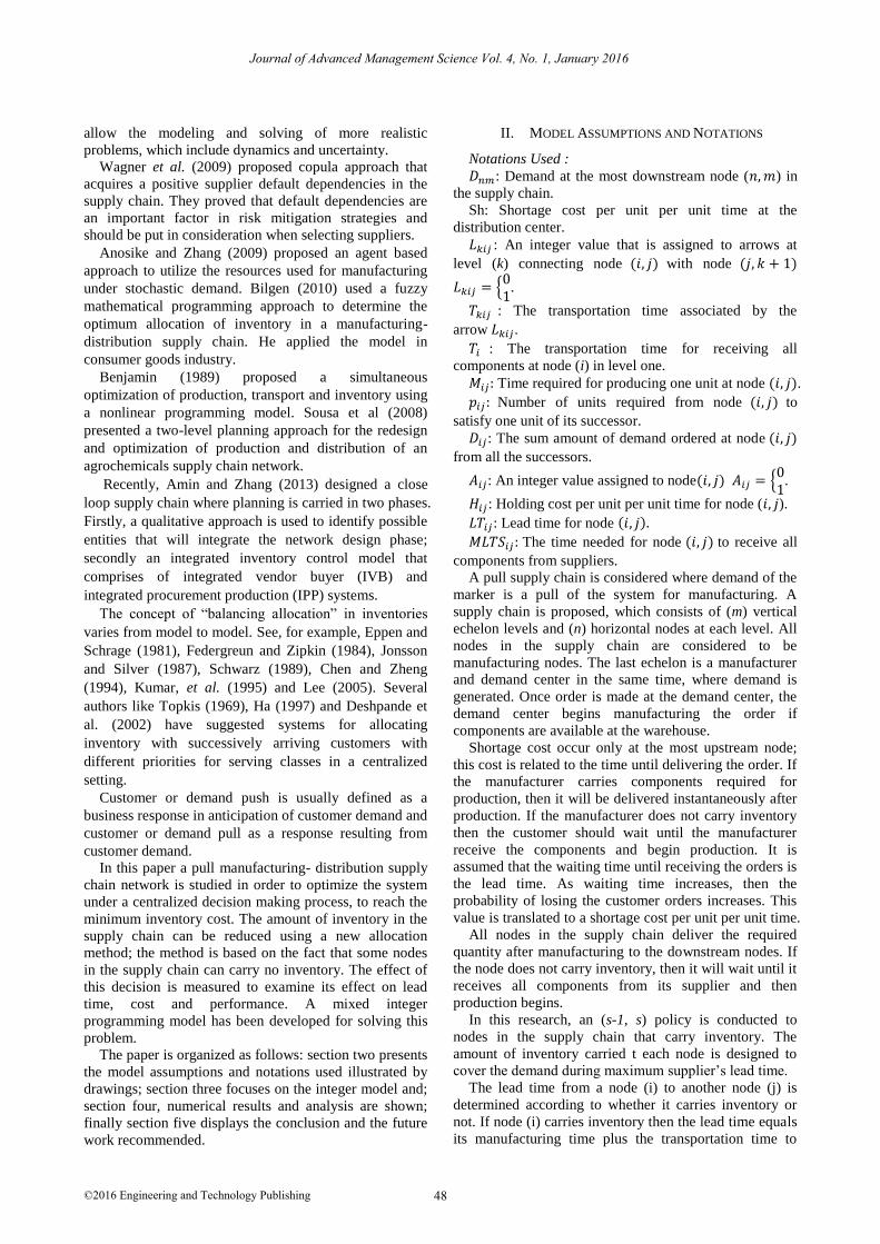
The supply chain is considered as network consisting

of nodes. Node’s location is determined by an (i) value

that determines its horizontal level and a (j) value that

determines its vertical level. An example is shown in Fig.

1.

Figure 1. Proposed supply chain structure

To figure axis labels, use words rather than symbols.

Do not label axes only with units. Do not label axes with

a ratio of quantities and units. Figure labels should be

legible, about 9-point type.

Color figures will be appearing only in online

publication. All figures will be black and white graphs in

print publication.

The location of each node in the supply chain is

determined by its value in the network. Arc

connecting different locations is determined by its

vertical location (L) in the supply and the two nodes from

the two ends. The symbol indicates the arc in level

one connecting between node (1, 1) and node (1, 2).

Arrow connects node and node .

An arrow ( ) either takes an integer value of {0 or

1}. If a zero is assigned to the arc, then there is no

connection between the nodes. If a one value is assigned

to the arc, then node is a supplier to node Each arrow holds information concerning the

transportation time to the predecessor node. The

transportation time ( ) on arc ( ) represents the unit

time for transporting products from node to

node . The transportation times to the nodes at

the first level ( ) are given by ).

Each node has an integer value ); whish either

takes the value {0 or 1}. The value zero indicates that this

node has warehouse and carry inventory. The value 1

indicated that no inventory is carried at this location.

Another value is assigned to each node ); which is

the time required to produce one unit of component. And

a value ) determines the number of units required by

manufacture to produce one unit of the most downstream

node demand.

The lead time of node is considered to be

the time required for manufacturing and receiving

components. In case the node carry inventory then it will

begin manufacturing directly, else it will wait until

components are received to begin production.

Each node has a Maximum Lead Time for its

Suppliers . This time determines the maximum

time for delivering all components, required for

manufacturing, to node The equals to the

maximum value of lead times of previous level,

plus its transportation time to node

III. MODEL IMPLEMENTATION

In this mode, the demand ( ) occurs only at the

most downstream node (demand center); this node is

considered to be manufacturer and distributor. The

shortage cost is assigned to this location as a function of

its lead time. Where (SH) is the shortage cost per unit per

unit time

(1)

The lead time ( ) for the demand center depends

on whether it has inventory or not. If it has inventory,

then the lead time equals to its manufacturing time. If it

does not have warehouse, and hence no inventory is

carried, then its lead time equals the maximum lead time

of its predecessors, plus the manufacturing time of the

required quantity. Since each node has different

transportation time to the demand center (most

downstream node) node, so there is no fixed value of lead

time to any successor. The determines the

maximum lead time of the suppliers to demand center,

which is equal to

{ } (2)

The lead time from the demand center to the customer

is the time required for the production of the ordered

amount, if the components are available; else it is

production time plus the lead time of its suppliers.

; (3)

Since each node has different transportation time to its

successor nodes, so there is no fixed value of lead time to

any successor. The ( ) determines the maximum

lead time of the suppliers to node including

transportation time to this node.

{ } (4)

Each node in the supply chain had a holding

cost ) per unit per unit time. The amount of inventory

carried at each location is supposed to be the quantity that

covers the lead time until orders are received from

supplier and then manufactured.

49



= ;

(5)

No holding cost will be incurred at a node that does not

carry inventory. While for nodes that carry inventory, the

holding cost will be the amount of inventory carried to

cover the demand during the . The is the

holding cost for the components required to produce one

unit demand ( per unit time.

(6)

The objective function for this model is to minimize

the total system cost. This cost consists of holding cost at

each node in the network, plus the shortage cost incurred

at the distribution center. The total cost is given by

∑∑

However, this system is constrained by several factors;

first, the demand at each node which is determined

according to the quantity ordered by its suppliers

(8)

Second, the lead times of nodes in level one of supply

chain are constrained by whether the node carry

inventory or not. This is shown in the next equation.

Max. { .

Max. { . .

Max. { .

Max. { (9)

Third factor is the maximum lead time of each node

from level ( ). The maximum lead time is

determined by

Max. {

(10)

The fourth factor is the lead time of the nodes from

level two to level (m) in the supply chain, lead time is

affected by whether it carries inventory or not. The lead

time equation for each node is given by

Max. {

Max. {

Max. {

Max. {

(11)

IV. NUMERICAL RESULTS

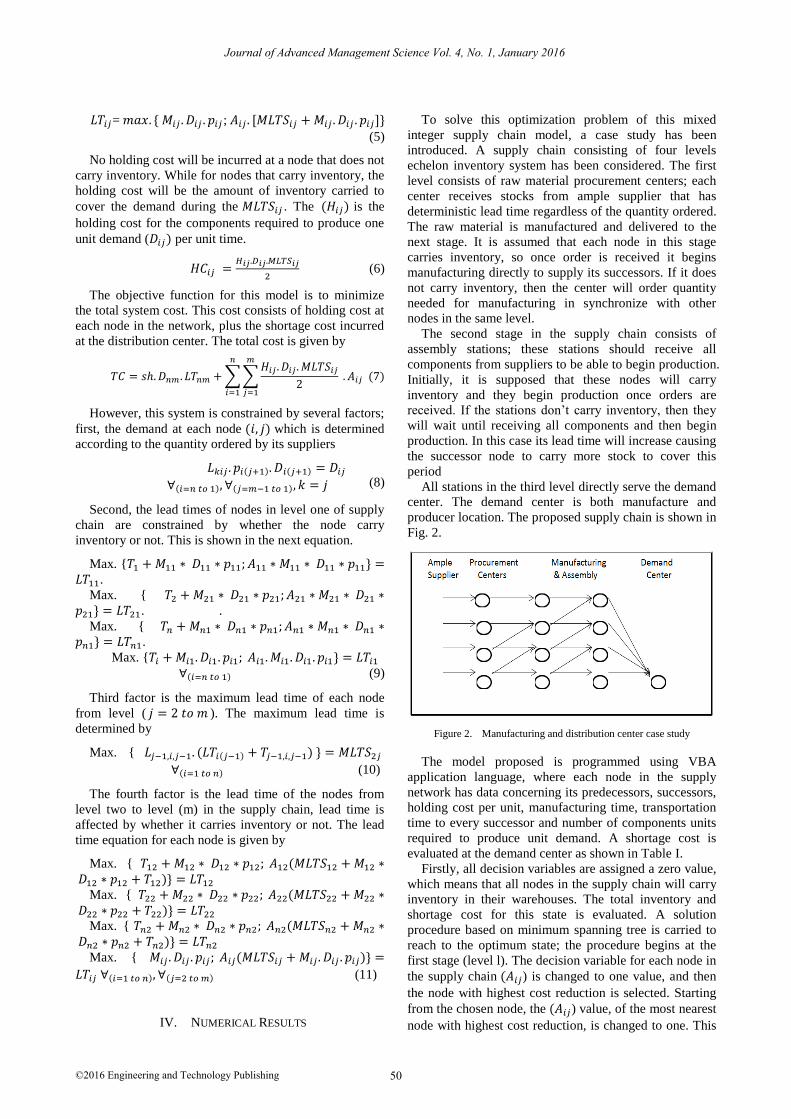
To solve this optimization problem of this mixed

integer supply chain model, a case study has been

introduced. A supply chain consisting of four levels

echelon inventory system has been considered. The first

level consists of raw material procurement centers; each

center receives stocks from ample supplier that has

deterministic lead time regardless of the quantity ordered.

The raw material is manufactured and delivered to the

next stage. It is assumed that each node in this stage

carries inventory, so once order is received it begins

manufacturing directly to supply its successors. If it does

not carry inventory, then the center will order quantity

needed for manufacturing in synchronize with other

nodes in the same level.

The second stage in the supply chain consists of

assembly stations; these stations should receive all

components from suppliers to be able to begin production.

Initially, it is supposed that these nodes will carry

inventory and they begin production once orders are

received. If the stations don’t carry inventory, then they

will wait until receiving all components and then begin

production. In this case its lead time will increase causing

the successor node to carry more stock to cover this

period

All stations in the third level directly serve the demand

center. The demand center is both manufacture and

producer location. The proposed supply chain is shown in

Fig. 2.

Figure 2. Manufacturing and distribution center case study

The model proposed is programmed using VBA

application language, where each node in the supply

network has data concerning its predecessors, successors,

holding cost per unit, manufacturing time, transportation

time to every successor and number of components units

required to produce unit demand. A shortage cost is

evaluated at the demand center as shown in Table I.

Firstly, all decision variables are assigned a zero value,

which means that all nodes in the supply chain will carry

inventory in their warehouses. The total inventory and

shortage cost for this state is evaluated. A solution

procedure based on minimum spanning tree is carried to

reach to the optimum state; the procedure begins at the

first stage (level l). The decision variable for each node in

the supply chain ) is changed to one value, and then

the node with highest cost reduction is selected. Starting

from the chosen node, the ) value, of the most nearest

node with highest cost reduction, is changed to one. This

50



process continues until reaching to the demand center,

and then repeated once more.

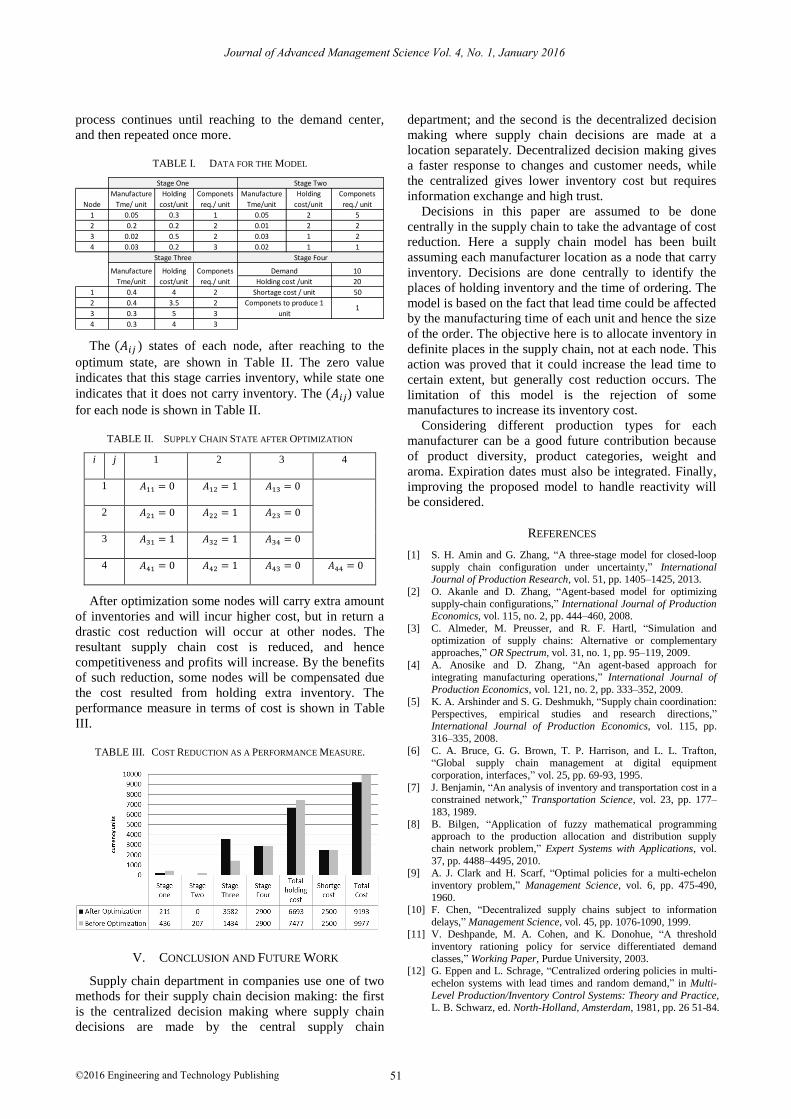
TABLE I. DATA FOR THE MODEL

The ) states of each node, after reaching to the

optimum state, are shown in Table II. The zero value

indicates that this stage carries inventory, while state one

indicates that it does not carry inventory. The ) value

for each node is shown in Table II.

TABLE II. SUPPLY CHAIN STATE AFTER OPTIMIZATION

i j 1 2 3 4

1

2

3

4

After optimization some nodes will carry extra amount

of inventories and will incur higher cost, but in return a

drastic cost reduction will occur at other nodes. The

resultant supply chain cost is reduced, and hence

competitiveness and profits will increase. By the benefits

of such reduction, some nodes will be compensated due

the cost resulted from holding extra inventory. The

performance measure in terms of cost is shown in Table

III.

TABLE III. COST REDUCTION AS A PERFORMANCE MEASURE.

V. CONCLUSION AND FUTURE WORK

Supply chain department in companies use one of two

methods for their supply chain decision making: the first

is the centralized decision making where supply chain

decisions are made by the central supply chain

department; and the second is the decentralized decision

making where supply chain decisions are made at a

location separately. Decentralized decision making gives

a faster response to changes and customer needs, while

the centralized gives lower inventory cost but requires

information exchange and high trust.

Decisions in this paper are assumed to be done

centrally in the supply chain to take the advantage of cost

reduction. Here a supply chain model has been built

assuming each manufacturer location as a node that carry

inventory. Decisions are done centrally to identify the

places of holding inventory and the time of ordering. The

model is based on the fact that lead time could be affected

by the manufacturing time of each unit and hence the size

of the order. The objective here is to allocate inventory in

definite places in the supply chain, not at each node. This

action was proved that it could increase the lead time to

certain extent, but generally cost reduction occurs. The

limitation of this model is the rejection of some

manufactures to increase its inventory cost.

Considering different production types for each

manufacturer can be a good future contribution because

of product diversity, product categories, weight and

aroma. Expiration dates must also be integrated. Finally,

improving the proposed model to handle reactivity will

be considered.

REFERENCES

[1] S. H. Amin and G. Zhang, “A three-stage model for closed-loop

supply chain configuration under uncertainty,” International Journal of Production Research, vol. 51, pp. 1405–1425, 2013.

[2] O. Akanle and D. Zhang, “Agent-based model for optimizing

supply-chain configurations,” International Journal of Production Economics, vol. 115, no. 2, pp. 444–460, 2008.

[3] C. Almeder, M. Preusser, and R. F. Hartl, “Simulation and

optimization of supply chains: Alternative or complementary approaches,” OR Spectrum, vol. 31, no. 1, pp. 95–119, 2009.

[4] A. Anosike and D. Zhang, “An agent-based approach for

integrating manufacturing operations,” International Journal of Production Economics, vol. 121, no. 2, pp. 333–352, 2009.

[5] K. A. Arshinder and S. G. Deshmukh, “Supply chain coordination:

Perspectives, empirical studies and research directions,” International Journal of Production Economics, vol. 115, pp.

316–335, 2008.

[6] C. A. Bruce, G. G. Brown, T. P. Harrison, and L. L. Trafton,

“Global supply chain management at digital equipment

corporation, interfaces,” vol. 25, pp. 69-93, 1995.

[7] J. Benjamin, “An analysis of inventory and transportation cost in a constrained network,” Transportation Science, vol. 23, pp. 177–

183, 1989.

[8] B. Bilgen, “Application of fuzzy mathematical programming approach to the production allocation and distribution supply

chain network problem,” Expert Systems with Applications, vol.

37, pp. 4488–4495, 2010. [9] A. J. Clark and H. Scarf, “Optimal policies for a multi-echelon

inventory problem,” Management Science, vol. 6, pp. 475-490,

1960. [10] F. Chen, “Decentralized supply chains subject to information

delays,” Management Science, vol. 45, pp. 1076-1090, 1999. [11] V. Deshpande, M. A. Cohen, and K. Donohue, “A threshold

inventory rationing policy for service differentiated demand

classes,” Working Paper, Purdue University, 2003. [12] G. Eppen and L. Schrage, “Centralized ordering policies in multi-

echelon systems with lead times and random demand,” in Multi-

Level Production/Inventory Control Systems: Theory and Practice, L. B. Schwarz, ed. North-Holland, Amsterdam, 1981, pp. 26 51-84.

1 0.05 0.3 1 0.05 2 5

2 0.2 0.2 2 0.01 2 2

3 0.02 0.5 2 0.03 1 2

4 0.03 0.2 3 0.02 1 1

10

20

1 0.4 4 2 50

2 0.4 3.5 2

3 0.3 5 3

4 0.3 4 3

1

Shortage cost / unit

Componets to produce 1

unit

Holding

cost/unit

Componets

req./ unit

Stage One Stage Two

Stage Three Stage Four

Demand

Holding cost /unit

Holding

cost/unit

Componets

req./ unit

Manufacture

Tme/unit

Manufacture

Tme/ unitNode

Holding

cost/unit

Componets

req./ unit

Manufacture

Tme/unit

51



[13] A. Federgruen and P. Zipkin, “Allocation policies and cost approximations for multi location production and inventory

problems,” Management Science, vol. 30, no. 1, pp. 69-84, 1984.

[14] K. Funaki, “Strategic safety stock placement in supply chain design with due-date based demand,” Int. J. Production

Economics, vol. 135, pp. 4–13, 2010.

[15] H. Jonsson and E. Silver, “Analysis of a two-echelon inventory-control system with complete redistribution,” Management

Science, vol. 33, no. 2, pp. 215-227, 1987.

[16] A. Kumar, L. B. Schwarz, and J. E. Ward, “Risk-pooling along a fixed delivery route using a dynamic inventory-allocation policy,”

Management Science, vol. 41, no. 2, pp. 344-362, 1995.

[17] M. T. Melo, S. Nickel, F. Saldanha-daGama, “Facility location and supply chain management—a review,” European Journal of

Operational Research, vol. 196, no. 2, pp. 401–412, 1991.

[18] T. Sawik, “Coordinated supply chain scheduling,” International Journal of Production Economics, vol. 120, pp. 437–451, 2009.

[19] L. B. Schwarz, “A model for assessing the value of warehouse

risk-pooling: Risk pooling over outside-supplier leadtimes,” Management Science, vol. 35, no. 7, pp. 828-842, 1989.

[20] S. S. Erenguç, N. C. Simpson, and A. J. Vakharia, “Integrated

production/distribution planning in supply chains: An invited review,” European Journal of Operational Research, vol. 115, pp.

219- 236, 1999.

[21] R. Sousa, N. Shah, and L. G. P. Georgiou, “Supply chain design and multilevel planning: An industrial case,” Computers &

Chemical Engineering, vol. 32, pp. 2643–2663, 2008.

[22] D. M. Topkis, “Optimal ordering and rationing policies in a non-stationary dynamic inventory model with n demand classes,”


[23] T. V. Vasilios, “Mathematical programming techniques to debottleneck the supply chain of fine chemical industries,”

Computers and Chemical Engineering, vol. 20, pp. S1269-S1274,

1996. [24] S. M. Wagner, C. Bode, and P. Koziol, “Supplier default

dependencies: Empirical evidence from the automotive industry,”

European Journal of Operational Research, vol. 199, no. 1, pp. 150–161, 2009.

[25] F. J. Williams, “Heuristic techniques for simultaneous scheduling

of production and distribution in multi-echelon structures: Theory and empirical comparisons,” Management Science, vol. 27, no. 3,

pp. 336-352, 1981.

[26] F. H. Williams, “A hybrid algorithm for simultaneous scheduling of production and distribution in multi-echelon structures,”


Bassem Roushdy is working as a lecturer in

the Department of Industrial Engineering in

the Arab Academy for Science and Technology, Cairo, Egypt. He is awarded his

Ph.D. form the Department of Mechanical

Engineering in Ain Shams University in 2012. Since that time he is working in the field of

supply chain optimization and jobs scheduling. Dr. Bassem has experience of

executive leadership in manufacturing,

supply chain management, quality control, continuous improvement and decision making.

52



Documents

Integer Programming Model for Inventory … Programming Model for Inventory Optimization for a Multi Echelon System . ... A supply chain network ... simulation models and abstract