Embed Size (px)
Citation preview

Master of Science ThesisStockholm, Sweden 2010
TRITA-ICT-EX-2010:305
W E I Z H E N M A
Instrumentation of Gait Analysis
K T H I n f o r m a t i o n a n d
C o m m u n i c a t i o n T e c h n o l o g y
Instrumentation of Gait Analysis
Weizhen Ma [email protected]
Master of Science Thesis 2010.12.8
Supervisor and Examiner: Prof. Gerald Q. Maguire Supervisor in Industry: Max J. Ortiz C.
Integrum AB
Kungliga Tekniska Högskolan (KTH)
Stockholm, Sweden
School of Information and Communication Technology, KTH
i
Abstract
This master’s thesis project “Instrumentation of Gait Analysis” was carried out at and funded by Integrum AB, Gothenburg, Sweden. Force analysis is critical during rehabilitation process of amputation patients, since overloading might place the bone-implant interface at risk; while underloading might extend unnecessarily the already long rehabilitation program [1]. Highly developed sensor and data acquisition technology provides an easy and reliable way to do force analysis. This thesis introduces the problem and provides background material regarding Orthotics and Prosthetics, including osseointegration. The existing gait analysis techniques and sensor technology will be described. Based upon the criteria that are introduced, a suitable sensor and integration platform was selected to implement a new gait analysis system. Several trials of different gait states are proposed using the prototype to do gait analysis, the results are presented and analyzed. The success of this prototype has lead to plans to design an Osseointegrated Prostheses for the Rehabilitation of Amputees(OPRA) product Keywords: Prosthetics, Osseointegration, Gait analysis, Sensor, Force analysis
School of Information and Communication Technology, KTH
ii
Abstrakt
Denna magisteruppsats projekt "Instrumentation av gånganalys" gjordes ut på och finansieras av Integrum AB, Göteborg, Sverige. Tryckmätning är kritisk under rehabiliteringsprocessen för amputation patienter, eftersom överbelastning kan innebära en ben-implantat gränssnitt på spel, medan underloading kan förlänga onödan redan långa rehabiliteringsprogram [1]. Högt utvecklade sensor och datainsamling teknik ger ett enkelt och tillförlitligt sätt att tvinga analys. Denna avhandling presenterar problemet och ger underlag för Ortopedteknik och proteser, inklusive osseointegration. Den befintliga gånganalys teknik och sensorteknik kommer att beskrivas. Grundval av de kriterier som introduceras, en lämplig sensor och integrationsplattform valdes att genomföra en ny gånganalys system. Flera försök med olika gångart stater föreslog att prototypen ska göra gånganalys är resultaten presenteras och analyseras. Framgången för denna prototyp har lett till planerar att konstruera en Osseointegrated Proteser för rehabilitering av Amputerade (OPRA) produkt Nyckelord: Proteser, Osseointegration, gånganalys, Sensor, tryckmätning
School of Information and Communication Technology, KTH
iii
Acknowledgements
I would like to warmly acknowledge Dr. Rickard Brånemark and Integrum AB in Gothenburg,
Sweden, for providing me with a wonderful opportunity and great financial support for my project.
I also want to especially thank Professor Gerald Q. Maguire Jr., who offered great help regarding
research methods and reviewing this thesis, and Mr. Max J. Ortiz C. who provided me with
necessary information about osseointegration prosthesis and valuable advice for both my hardware
design and my documentation of this system. Additionally, I thank the National Library of
Medicine (NLM), USA for providing the gait cycle image in Chapter 2.
I also received help from Professor Mark T. Smith, Mr. Thomas Nilsson, and my friend Dandan
Wei, my sincere thanks to you all.

School of Information and Communication Technology, KTH
iv
Table of Content
Abstract………………………………………………………………………………………………………………………………………..i
Abstrakt ............................................................................................................................................. ii
Acknowledgements .......................................................................................................................... iii
List of Figures ................................................................................................................................... vi
List of Tables ................................................................................................................................... viii
List of Acronyms and Abbreviations ................................................................................................. ix
Chapter 1. Introduction ..................................................................................................................... 1
1.1 Background ................................................................................................................... 1
1.2 Osseointegration and Integrum AB ............................................................................... 2
1.3 Project Proposal ............................................................................................................... 2
1.4 Project Organization ......................................................................................................... 3
1.5 Methods and Thesis Structure ............................................................................................ 4
Chapter 2. Review of Instrumented Gait Analysis ............................................................................. 5
Chapter 3. Selection of Sensors ........................................................................................................ 7
3.1 Force Sensor Review ..................................................................................................... 7
3.1.1 Theoretical Background ........................................................................................ 7
3.1.2 Structure of a Piezoelectric Sensor ....................................................................... 8
3.2 Sensor Selection ............................................................................................................ 9
3.3 Sensor Calibration ....................................................................................................... 10
Chapter 4. System Design and Implementation .............................................................................. 14
4.1 Integration Platform ....................................................................................................... 14
4.1.1 Platform Selection ............................................................................................... 15
4.1.2 Microcontroller and Board Features ................................................................... 16
4.2 Hardware Implementation ............................................................................................. 17
4.2.1 Driver Circuit Implementation ................................................................................ 17
4.2.2 Physical Packaging of the Device ............................................................................ 19
4.3 Device Fixture ................................................................................................................. 21
4.4 Software Design ............................................................................................................. 22

School of Information and Communication Technology, KTH
v
4.4.1 ADC Configuration .................................................................................................. 22
4.4.2 PC Application ........................................................................................................ 23
4.5 Data Format ...................................................................................................................... 24
4.6 System Test ........................................................................................................................ 26
4.6.1 Measurement Test ................................................................................................. 26
4.6.2 Power Consumption ............................................................................................... 27
Chapter 5. Trials .............................................................................................................................. 28
5.1 Methods ............................................................................................................................ 28
5.2 Trial of Standing State ....................................................................................................... 29
6.3 Dynamic Trials ............................................................................................................. 30
5.3.1 Straight Walking Trial.............................................................................................. 30
5.3.2 Turning Trial ............................................................................................................ 32
5.3.3 Jumping Trial .......................................................................................................... 33
Chapter 6. Analysis and Results ...................................................................................................... 34
6.1 Standing State Analysis ..................................................................................................... 34
6.2 Dynamic Gait Analysis ....................................................................................................... 38
6.2.1 Straight Walking Analysis ....................................................................................... 38
6.2.2 Turning Analysis ...................................................................................................... 39
6.2.3 Jumping Analysis .................................................................................................... 40
Chapter 7. Discussions .................................................................................................................... 42
7.1 Discussion of Environmental Factors ................................................................................. 42
7.2 Comparison ....................................................................................................................... 44
7.2.1 F-Scan® System Applications ................................................................................... 44
7.2.2 Gait Analysis in Medical Care ................................................................................. 44
7.2.3 Extensive Studies .................................................................................................... 45
Chapter 8 Conclusions ..................................................................................................................... 46
8.1 Conclusions ....................................................................................................................... 46
8.2 Future Work ...................................................................................................................... 47
References ...................................................................................................................................... 48
School of Information and Communication Technology, KTH
vi
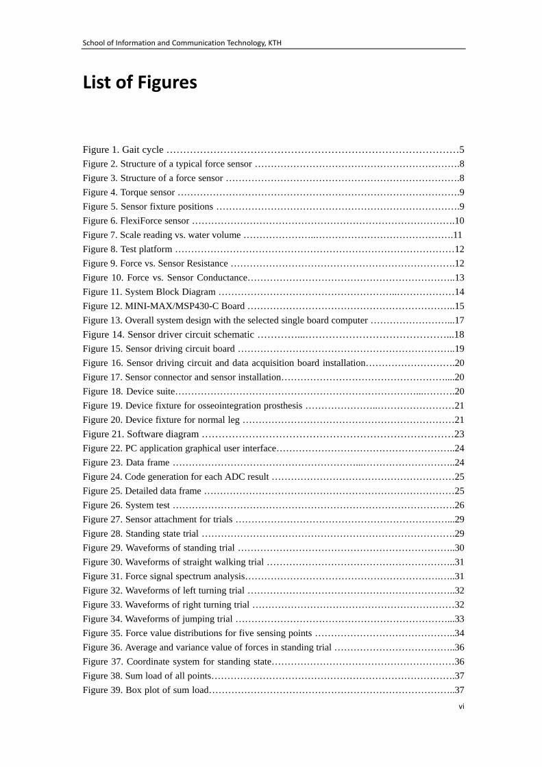
List of Figures
Figure 1. Gait cycle ……………………………………………………………………………5 Figure 2. Structure of a typical force sensor ……………………………………………………….8 Figure 3. Structure of a force sensor ……………………………………………………………….8 Figure 4. Torque sensor …………………………………………………………………………….9 Figure 5. Sensor fixture positions ………………………………………………………………….9 Figure 6. FlexiForce sensor ……………………………………………………………………….10 Figure 7. Scale reading vs. water volume …………………..…………………………………….11 Figure 8. Test platform ……………………………………………………………………………12 Figure 9. Force vs. Sensor Resistance …………………………………………………………….12 Figure 10. Force vs. Sensor Conductance………………………………………………………..13 Figure 11. System Block Diagram ………………………………………………..………………14 Figure 12. MINI-MAX/MSP430-C Board ………………………………………………………..15 Figure 13. Overall system design with the selected single board computer ……………………...17 Figure 14. Sensor driver circuit schematic …………...……………………………………...18 Figure 15. Sensor driving circuit board …………………………………………………………..19 Figure 16. Sensor driving circuit and data acquisition board installation……………………….20 Figure 17. Sensor connector and sensor installation……………………………………………....20 Figure 18. Device suite…………………………………………………………………...……….20 Figure 19. Device fixture for osseointegration prosthesis …………………..……………………21 Figure 20. Device fixture for normal leg …………………………………………………………21 Figure 21. Software diagram …………………………………………………………………23 Figure 22. PC application graphical user interface………………………………………………..24 Figure 23. Data frame …………………………………………………...………………………..24 Figure 24. Code generation for each ADC result …………………………………………………25 Figure 25. Detailed data frame ……………………………………………………………………25 Figure 26. System test …………………………………………………………………………….26 Figure 27. Sensor attachment for trials …………………………………………………………...29 Figure 28. Standing state trial …………………………………………………………………….29 Figure 29. Waveforms of standing trial …………………………………………………………..30 Figure 30. Waveforms of straight walking trial …………………………………………………..31 Figure 31. Force signal spectrum analysis…………………………………………………….…..31 Figure 32. Waveforms of left turning trial ………………………………………………………..32 Figure 33. Waveforms of right turning trial ………………………………………………………32 Figure 34. Waveforms of jumping trial …………………………………………………………...33 Figure 35. Force value distributions for five sensing points ……………………………………..34 Figure 36. Average and variance value of forces in standing trial ………………………………..36 Figure 37. Coordinate system for standing state…………………………………………………36 Figure 38. Sum load of all points………………………………………………………………….37 Figure 39. Box plot of sum load…………………………………………………………………..37
School of Information and Communication Technology, KTH
vii
Figure 40. Maximum and average values of forces in walking trial ……………………………...38 Figure 41. Maximum and average values of forces in left turning trial …………………………..39 Figure 42. Maximum and average values of forces in right turning trial ………………………...40 Figure 43. Maximum and average values of forces in forefoot contacting first jumping trial …...41 Figure 44. An experiment for rigid contact surfaces………………………………………………42 Figure 45. Walking trial results comparison………………………………………………………43

School of Information and Communication Technology, KTH
viii
List of Tables
Table 1. Break points for titanium fixture ………………………………………………………….3 Table 2. FlexiForce® A201 Specification ………………………………………………………...10 Table 3. Specification of BOLMEN IKEA Scale …………………………………………………11 Table 4. Feature of MSP430 ………………………………………………………………………16 Table 5. MINI-MAX/MSP430-C Specification …………………………………………………..16 Table 6. System test analysis ……………………………………………………………………...27 Table 7. Relevant sample physical condition ……………………………………………………..28 Table 8. Standing trial descriptive statistics …………...…………….……………………………36 Table 9. Maximum and average values of peak forces in walking trial …………………………..38 Table 10. Maximum and average values of peak forces in left turning trial ……………………...39 Table 11. Maximum and average values of peak forces in right turning trial …………………….40 Table 12. Maximum and average values of peak forces in forefoot first jumping trial …………..41 Table 13. Peak plantar pressure for 0kg load during walking……………………………..………43

School of Information and Communication Technology, KTH
ix
List of Acronyms and Abbreviations
2-D 2-Dimensional 3-D 3-Dimensional ADC Analog to Digital Converter BIOPAC BIOPAC Systems, Inc. BMI Body Mass Index BiPOM BiPOM Electronics Inc. CPU Central Processing Unit Chk Check sum byte EEM Embedded Emulation Module F-Scan® F-Scan in-shoe plantar pressure measurement system FES Functional Electrical Simulation FPI-6 Foot Posture Index FSR Force Sensing Resistor FTDI Future Technology Devices International Hz Hertz, unit of frequency I2C, Inter-Integrated Circuit IrDA Infrared Data Association JTAG Joint Test Action Group KB KiloByte KHz Kilo Hertz, unit of frequency KPa KiloPascal, unit of pressure Kohm KiloOhm, unit of resistance MHz Mega Hertz MTH1 Meta Tarsal Head 1 MTH3 Meta Tarsal Head 3 MTH5 Meta Tarsal Head 5 N Newton, unit of force NADC Result generated by Analog to Digital Converter OPRA Osseointegrated Prostheses for the Rehabilitation of Amputees PC Personal Computer R Resistor RAM Random Access Memory RISC Reduced Instruction Set Computer RS232 Recommended Standard 232 RTS/CTS Request To Send/Clear To Send Rf Feedback Resistance Rs Sensor’s Resistance SD Standard Deviation SEN1 Sensor wire pad 1 SEN2 Sensor wire pad 2
School of Information and Communication Technology, KTH
x
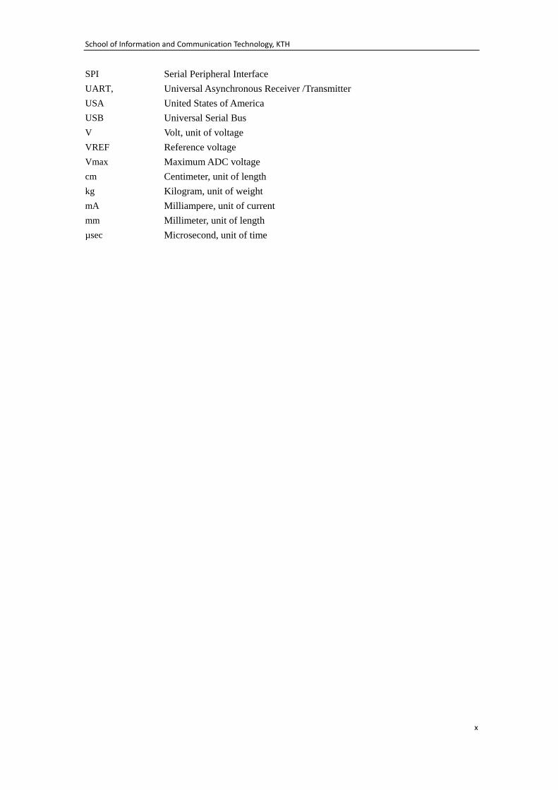
SPI Serial Peripheral Interface UART, Universal Asynchronous Receiver /Transmitter USA United States of America USB Universal Serial Bus V Volt, unit of voltage VREF Reference voltage Vmax Maximum ADC voltage cm Centimeter, unit of length kg Kilogram, unit of weight mA Milliampere, unit of current mm Millimeter, unit of length µsec Microsecond, unit of time
School of Information and Communication Technology, KTH
1
Chapter 1. Introduction
1.1 Background
Orthotics and prosthetics science is one of the most intimate meeting points between technology and human beings. The term orthotics is defined as “The field of design and fabrication of the devices to replace a body part”[2]. While the term prosthetics is defined as “The field of design and fabrication of any type of brace device” [2]. Amputation is the removal of a limb or other appendage or outgrowth of the body. Amputation frequently requires support from orthotics and prosthetics technology. These technologies enable the design and manufacture of safe, stable, and comfortable prostheses. Because “Amputation produces a deep physical and emotional response in the patient” [3], good prosthesis design helps amputees to live normal lives and regain their confidence. Lower limb amputations appear most frequently in medical amputation cases, “ There are at least 10 times more lower extremity amputations than there are upper extremity amputations” (in the US) [2]. A Lower Limb Amputation can be further classified as Syme’s, Transtibial, knee disarticulation, transfemoral, and hip disarticulation. Syme’s amputation removes the medial and lateral malleolus. While transtibial is the removal of the limb above the foot and below knee. Transfemoral is the amputation of the limb between knee and hip. Hip disarticulation removes whole lower limb including hip. There are various differences between these amputations for prosthesis designers regarding energy cost or force conduction. Because of these factors, well-designed or anatomical prostheses are highly desired by the Lower Limb Amputation patients. However, Pawlikowski, et al. point out that “a high number of custom-designed prostheses are prone to failure” due to designers’ limited “experience and knowledge of load transfer mechanism”[4]. As a consequence, it is necessary to analyze the force and load that will be applied to the prosthesis during the prosthesis design process. According to Florschutz, et al. study of osseointegrated tantalum implants, mechanical testing and histology shows tighter implant fixation over time, but “the implants had stiffness and maximum torque to failure measurements that were significantly lower than intact controls”.[5] The goal of this thesis project is to exploit highly developed modern sensor and mobile computing technologies to provide a method and tool to analyze the force and load on a prosthesis in a simple and reliable way.

School of Information and Communication Technology, KTH
2
1.2 Osseointegration and Integrum AB
For lower limb amputation patients, traditional socket prostheses tend to wear out after a period of wearing. The femoral head penetrates the polyethylene socket by 0.1 mm/year (in the case of a ceramic femoral head on polyethylene) and 0.2-0.6mm/year (in the case of a metal on polyethylene)[6]. In Hagberg et al. a study on hip range of motion, a transfemoral prosthetic socket significantly reduces the range of motion of the hip and an increase in discomfort when sitting is common among individuals wearing such prostheses[7]. In the 1950s, Per-Ingvar Brånemark studied the long-term stability of titanium implants in the canine jaw, and discovered that the titanium implants can be integrated into bone tissue[8]. Brånemark introduced the term “osseointegration” to describe the phenomenon. Osseointegration is defined as continuing structural and functional coexistence, possibly in a symbiotic manner, between differentiated, adequately remodeled, biologic tissues and strictly defined and controlled synthetic components, providing lasting, specific clinical functions without initiating rejection mechanisms[9]. Studies show that individuals wearing a bone-anchored prosthesis do not have restricted hip motion with the prosthesis and few have problems with discomfort when sitting[7]. Treatment with osseointegrated transfemoral prostheses have been shown to improve the patients’ quality of life. During the period 1990 to June 2008, 100 transfemoral amputation cases with 106 limbs have been treated in Sahlgrenska University Hospital Gothenburg, Sweden [10]. Integrum AB, a Swedish medical technology company develops devices for direct skeletal anchorage of amputation prostheses. This firm was founded by Richard Brånemark (the son of P.I. Brånemark) in 1998. The main product of the company is their Osseointegrated Prostheses for the Rehabilitation of Amputees system. This system consists of an anchoring element which is surgically inserted into the bone of the amputation stump. The outer part of the abutment is connected to the skin penetrating component that is attached to the fixture. [11]
1.3 Project Proposal
In the osseointegration process, there are typically two phases. In the first phase, the fixtures are installed in the bone tissue, then remain unloaded for healing for a period of 3-6 months, then in the second phase, the fixtures are connected to a superstructure and loaded[12]. The purpose of first phase is to enable the structural and functional connection of the fixture into the bone via the healing process, nevertheless, there exist breaking points with respect to both torques and pull-out or bending forces applying to the fixtures. In the study of rats, the break point values also vary in different periods of the healing. This is shown in Table 1.

School of Information and Communication Technology, KTH
3
Table 1. Break points for titanium fixture (Source from [12] Table 1. Mean, range and sample size for mechanical and histomorphometric results, by healing time) 0 week 2 weeks 4 weeks 8 weeks 16 weeks
Break point troque (10-3 Nm)
24 19 20 30.4 50.8
Pull-out load (N) 32.6 55.2 81.5 93.4 104.8
As it would be unethical to perform such experiments on human patients, it is desirable to monitor and record the biomechanical forces on the prostheses during patients’ daily activities, in which the most common one is gait (A definition of gait and further details about gait analysis are given in Chapter 2). This data can be used to support the rehabilitation process. Frossard L. et al. point that after second surgery of osseointegration in lower limb amputation, the patients have to perform an extensive rehabilitation program “including, but not limited to, static load bearing exercises” and “applying suitable stress during this period is critical” because “overloading might place the bone-implant interface at risk while underloading might extend unnecessarily the already long rehabilitation program.” The force data can also be used in the following dynamic load bearing exercises.[1] Furthermore, since the mechanical characteristics and forces on the prostheses would affect the level of comfort, range of motion, and the safety of the patients, it is desirable to have a device that can measure and record biomechanical data from the prostheses for further optimization and development of future prosthesis, as well as to potentially warn the patient if they are approaching the limits of their prosthesis. This project will develop a stand-alone system that can be worn by a trans-femoral amputation patient without compromising the mechanical integrity of the prosthesis. This device should be able to record forces exerted by the foot to the ground during gait. The data should be transmitted to a remote computer where it is displayed in real-time. Additionally, the system will acquire and store the force data in a portable memory card which is inserted in the device itself.
1.4 Project Organization
This project was funded by Integrum AB, Gothenburg, Sweden as a master’s thesis project at Royal Institute of Technology(KTH), Stockholm under the supervision of a bionics engineer from Integrum AB and professor from KTH. The timeline of this project was divided into five phases: 1. Research on the relevant current state-of-art and commercially available products 2. System design (in term of structure and function) 3. Implementation 4. Testing and calibration 5. Trials and analysis 6. Project presentation in both oral and written forms

School of Information and Communication Technology, KTH
4
The necessary information about the osseointegrated prosthesis and equipment were provided by Integrum AB. The testing was done using mechanical loads and did not involve any patients.
1.5 Methods and Thesis Structure
A brief review of relevant literatures was performed at the first phase of this project, it leaded to a clear scope identification and deep understanding of our topic “instrumentation of gait analysis”. A possible solution was proposed after the literature study. In the second phase, suitable materials and products were selected and purchased, after which the system was designed and implemented. Several trials related to gait analysis were conducted using developed prototype. According to the quantitative analysis of the samples collected from the trials, the results were given and discussed. Conclusion provided the summary of the system including pros and cons, followed by future work. This structure of this thesis report is as following. Review of instrumentation of gait analysis Selection of sensors System design and implementation Trials Analysis and results Discussions Conclusions and future work
School of Information and Communication Technology, KTH
5
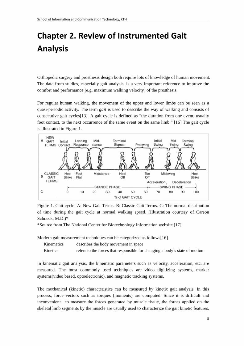
Chapter 2. Review of Instrumented Gait Analysis Orthopedic surgery and prosthesis design both require lots of knowledge of human movement. The data from studies, especially gait analysis, is a very important reference to improve the comfort and performance (e.g. maximum walking velocity) of the prosthesis. For regular human walking, the movement of the upper and lower limbs can be seen as a quasi-periodic activity. The term gait is used to describe the way of walking and consists of consecutive gait cycles[13]. A gait cycle is defined as “the duration from one event, usually foot contact, to the next occurrence of the same event on the same limb.” [16] The gait cycle is illustrated in Figure 1.
Figure 1. Gait cycle: A: New Gait Terms. B: Classic Gait Terms. C: The normal distribution of time during the gait cycle at normal walking speed. (Illustration courtesy of Carson Schneck, M.D.)* *Source from The National Center for Biotechnology Information website [17]
Modern gait measurement techniques can be categorized as follows[16].
Kinematics describes the body movement in space Kinetics refers to the forces that responsible for changing a body’s state of motion
In kinematic gait analysis, the kinematic parameters such as velocity, acceleration, etc. are measured. The most commonly used techniques are video digitizing systems, marker systems(video based, optoelectronic), and magnetic tracking systems. The mechanical (kinetic) characteristics can be measured by kinetic gait analysis. In this process, force vectors such as torques (moments) are computed. Since it is difficult and inconvenient to measure the forces generated by muscle tissue, the forces applied on the skeletal limb segments by the muscle are usually used to characterize the gait kinetic features.
School of Information and Communication Technology, KTH
6
Force platform systems are commonly used to measure the foot pressure against the ground. These measurements play an important role in ankle prosthesis design. Sensor based systems are most popular method of making force measurements of the upper or lower limbs prosthesis. This project does kinetic gait analysis based on a sensor system. There have been a lot of research experiments concerning prosthesis gait analysis. For example, S. Ingrosso et al. did gait analysis of an ankle prosthesis, in which the moments are measured and analyzed[18]; A. Merkur et al. investigated both kinematic and kinetic characteristics of an ankle food prosthesis during stair gaiting[19]; A. Boonstra et al. analyzed and compared two knee units[20]; and Åström and Stenström use questionnaires to study socket comfort in gait[21]. Instrumented gait analysis is becoming more and more important in gait event detection and clinical application. As stated by J. Rueterbories et al., “nowadays, the input data is obtained by electronic sensors that measure various parameters during the gait cycle” [13]. They also point out that “restoration of walking can be supported by functional electrical simulation (FES) which has become an accepted rehabilitation method”. [13] According to Rueterbories, “a number of methods for gait measurements are based on the force exerted by the body to the ground” and the position for sensors is “between the sole of foot and the ground.”[13] As an example, H. Wang et al. developed “a novel 3D platform system suitable for the measurement of human foot pressure distribution.” [14] They use ultra-thin, grid-based sensor arrays to measure the vertical force while using rows of conductors and semiconductors that are vertically laid on the surface of sensors to measure the horizontal forces. Another system using force sensing resistor is designed by Rana, he uses FSR sensors to measure the force against the ground by attaching them to the bottom of a shoe mat. Several measurement points are selected in order to measure peak force, the system was integrated with a BIOPAC MP100 data acquiring system and connected to a computer[15]. A method similar to Rana’s will be used in this project to perform force analysis. However, instead of using an expensive and general purpose data acquisition system, a dedicated data acquisition and storage system will be developed so that the final system will be more portable and much lower in cost.

School of Information and Communication Technology, KTH
7
Chapter 3. Selection of Sensors
For gait measurements that are based on the force exerted by the body to the ground, Rueterbories et al. point out that “the only possible position for the sensors is therefore between the sole of the foot and the ground”, the sensors are transducers which can be “mechanical, load dependent switches, capacitive or piezoelectric elements”[13].
3.1 Force Sensor Review
For robotic sensing, mainly two types of sensors are used: internal state sensors and external state sensors. External state sensors are “used to monitor the geometric and/or dynamic relation between robot and its task, environment, or the object that is handling. [22]” The most commonly used force sensors are made of piezoelectrical materials, the theory will be discussed in the following subsection. A sensor utilizing applying piezoelectricity can be extremely thin and sensitive.
3.1.1 Theoretical Background
Jacques and Pierre Curie discovered an special effect applying mechanical forces on certain type of crystal, the crystal became polarized electrically, and generated voltages of the opposite polarity proportional to the applied force. This effect was called the piezoelectric effect. Since then, piezoelectric materials have been commonly used in the power supplies [23], electrical measurement (microelectromechanical systems [24]), sensors (piezoresistive force sensors[25]), motors[26], frequency standards [27], etc. In classical piezoelectricity, the anisotropic resistivity tensor 𝜌 can be expressed as in equation (1) in terms of stress vector (ϭ), piezoresistive tensor (П), elasticity tensor (D), and strain vector (ε)[25]. 𝜌 = 𝜌�{𝐼� + П ϭ} = 𝜌�{𝐼� + П𝐷𝜀} (1) Where ϭ = 𝐷𝜀. From equation(1), the resistivity tensor is determined by the material stresses value. 𝐸 = 𝜌𝐽 (2) 𝐸 = −𝛻∅ (3)
School of Information and Communication Technology, KTH
8
Solving the simultaneous equations (2) and (3), the electric potential ∅ (corresponding to the electric field) and resistivity tensor 𝜌 (the mechanical stress applied on the material) can be related, therefore by measuring the electric potential we can measure the anisotropic resistivity tensor and based upon the known properties of the material we can compute the force vector.
3.1.2 Structure of a Piezoelectric Sensor
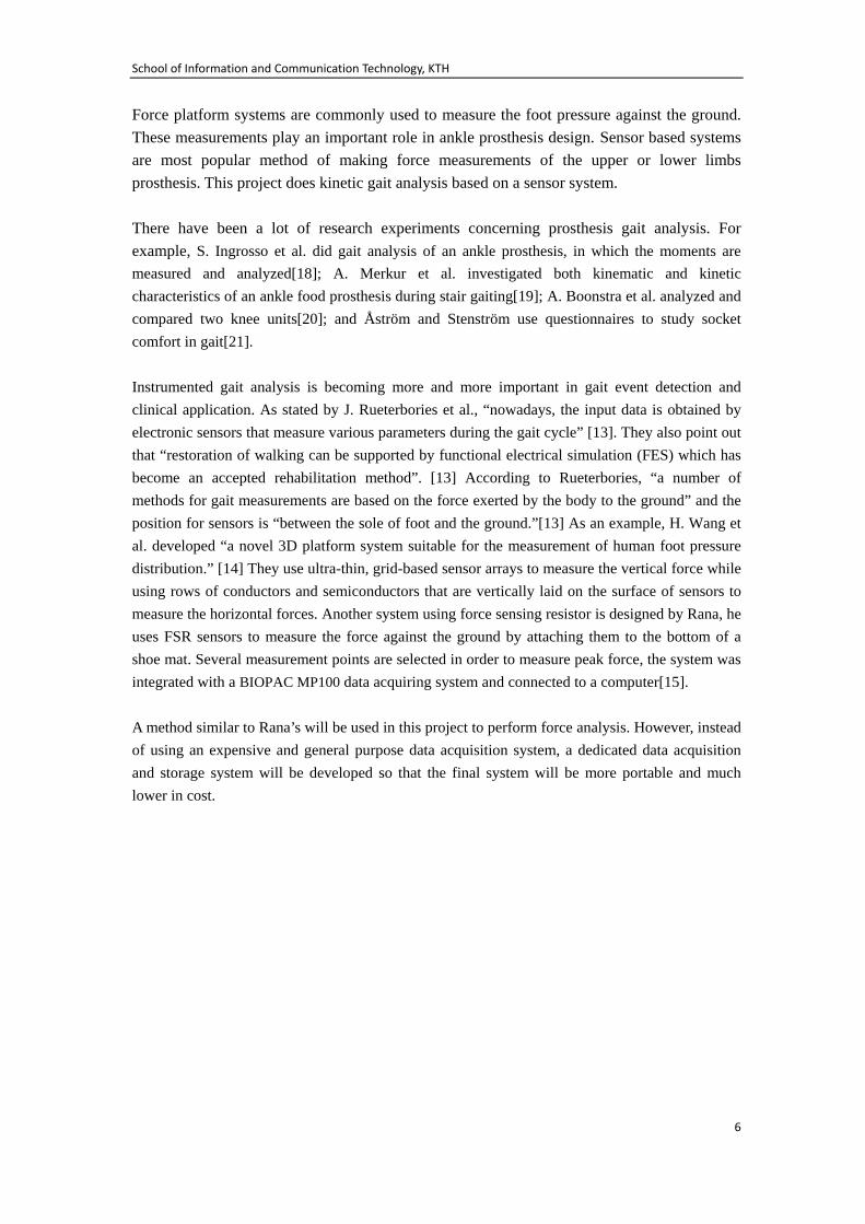
Piezoresistivity is commonly used in electronic measurements utilizing piezoelectric quartz crystals. A change in the mechanical stress on the crystal causes a change in the material’s resistivity, which can be measured by applying and electrical potential and then using Ohm’s Law [28]. The structure of a typical piezoelectric sensor [29] is shown in Figure 2.
Figure 2. Structure of a typical force sensor A charge-collection electrode is located between two crystal materials. The housing provides the other electrode. The voltage generated by the compressed quartz is used to sense the force applied to the quartz. When applying a vertical force on the impact cap of the Figure 2. The double-layer quartz structure will generate an electric potential between the electrodes and this voltage will be routed to an amplifier. The stud preloads are used to provide a stable initial state for the sensor by assure close contact of all parts.
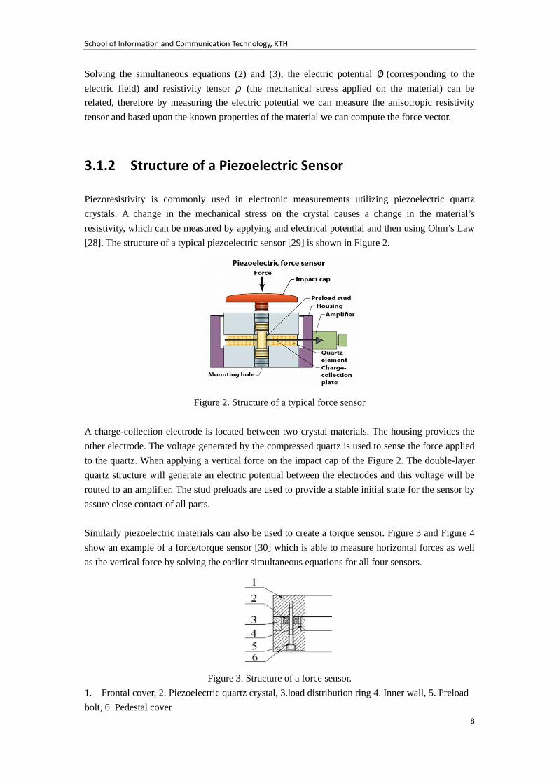
Similarly piezoelectric materials can also be used to create a torque sensor. Figure 3 and Figure 4 show an example of a force/torque sensor [30] which is able to measure horizontal forces as well as the vertical force by solving the earlier simultaneous equations for all four sensors.
Figure 3. Structure of a force sensor.
1. Frontal cover, 2. Piezoelectric quartz crystal, 3.load distribution ring 4. Inner wall, 5. Preload bolt, 6. Pedestal cover
School of Information and Communication Technology, KTH
9
Figure 4. Torque sensor
3.2 Sensor Selection
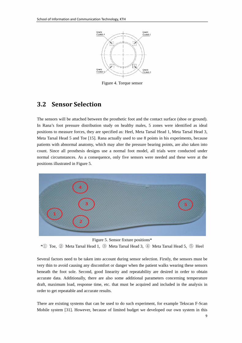
The sensors will be attached between the prosthetic foot and the contact surface (shoe or ground). In Rana’s foot pressure distribution study on healthy males, 5 zones were identified as ideal positions to measure forces, they are specified as: Heel, Meta Tarsal Head 1, Meta Tarsal Head 3, Meta Tarsal Head 5 and Toe [15]. Rana actually used to use 8 points in his experiments, because patients with abnormal anatomy, which may alter the pressure bearing points, are also taken into count. Since all prosthesis designs use a normal foot model, all trials were conducted under normal circumstances. As a consequence, only five sensors were needed and these were at the positions illustrated in Figure 5.
Figure 5. Sensor fixture positions*
*① Toe, ② Meta Tarsal Head 1, ③ Meta Tarsal Head 3, ④ Meta Tarsal Head 5, ⑤ Heel
Several factors need to be taken into account during sensor selection. Firstly, the sensors must be very thin to avoid causing any discomfort or danger when the patient walks wearing these sensors beneath the foot sole. Second, good linearity and repeatability are desired in order to obtain accurate data. Additionally, there are also some additional parameters concerning temperature draft, maximum load, response time, etc. that must be acquired and included in the analysis in order to get repeatable and accurate results. There are existing systems that can be used to do such experiment, for example Tekscan F-Scan Mobile system [31]. However, because of limited budget we developed our own system in this
School of Information and Communication Technology, KTH
10
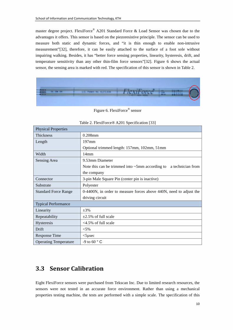
master degree project. FlexiForce® A201 Standard Force & Load Sensor was chosen due to the advantages it offers. This sensor is based on the piezoresistive principle. The sensor can be used to measure both static and dynamic forces, and “it is thin enough to enable non-intrusive measurement”[32], therefore, it can be easily attached to the surface of a foot sole without impairing walking. Besides, it has “better force sensing properties, linearity, hysteresis, drift, and temperature sensitivity than any other thin-film force sensors”[32]. Figure 6 shows the actual sensor, the sensing area is marked with red. The specification of this sensor is shown in Table 2.
Figure 6. FlexiForce® sensor
Table 2. FlexiForce® A201 Specification [33]
Physical Properties Thickness 0.208mm Length 197mm
Optional trimmed length: 157mm, 102mm, 51mm Width 14mm Sensing Area 9.53mm Diameter
Note this can be trimmed into ~5mm according to a technician from the company
Connector 3-pin Male Square Pin (center pin is inactive) Substrate Polyester Standard Force Range 0-4400N, in order to measure forces above 440N, need to adjust the
driving circuit Typical Performance Linearity ±3% Repeatability ±2.5% of full scale Hysteresis <4.5% of full scale Drift <5% Response Time <5µsec Operating Temperature -9 to 60 ° C
3.3 Sensor Calibration
Eight FlexiForce sensors were purchased from Tekscan Inc. Due to limited research resources, the sensors were not tested in an accurate force environment. Rather than using a mechanical properties testing machine, the tests are performed with a simple scale. The specification of this
School of Information and Communication Technology, KTH
11
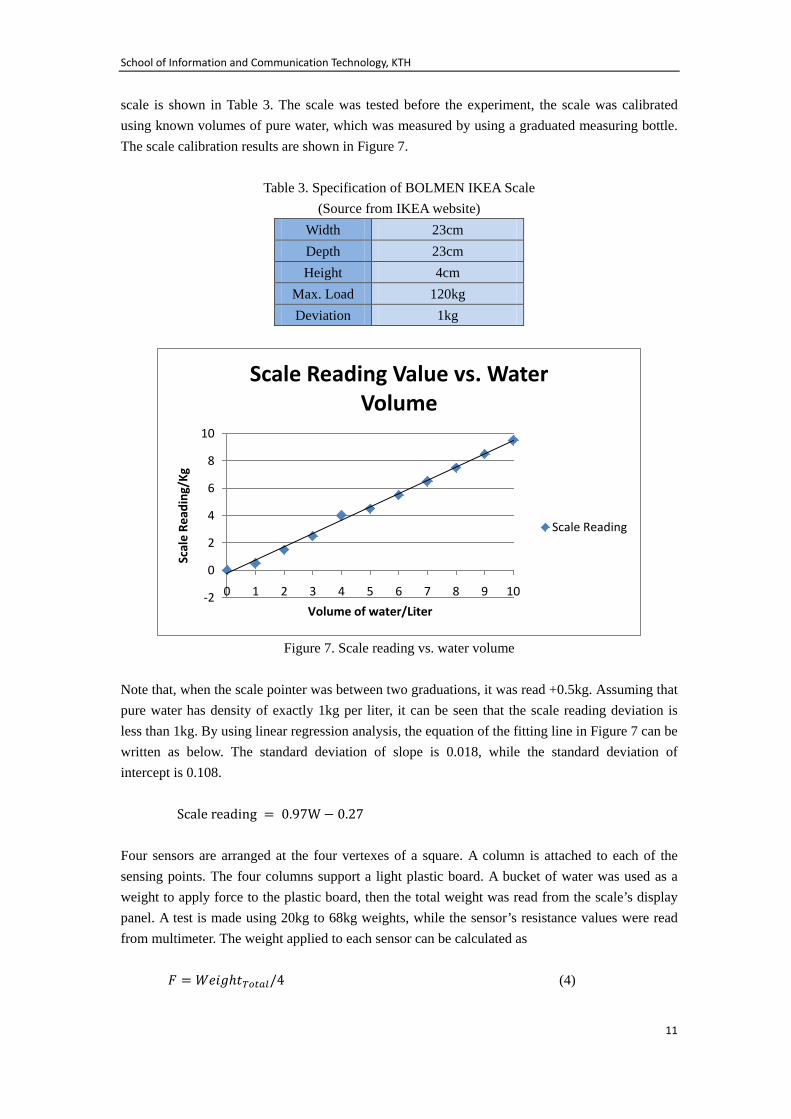
scale is shown in Table 3. The scale was tested before the experiment, the scale was calibrated using known volumes of pure water, which was measured by using a graduated measuring bottle. The scale calibration results are shown in Figure 7.
Table 3. Specification of BOLMEN IKEA Scale (Source from IKEA website)
Width 23cm Depth 23cm Height 4cm
Max. Load 120kg Deviation 1kg
Figure 7. Scale reading vs. water volume
Note that, when the scale pointer was between two graduations, it was read +0.5kg. Assuming that pure water has density of exactly 1kg per liter, it can be seen that the scale reading deviation is less than 1kg. By using linear regression analysis, the equation of the fitting line in Figure 7 can be written as below. The standard deviation of slope is 0.018, while the standard deviation of intercept is 0.108. Scale reading = 0.97W − 0.27 Four sensors are arranged at the four vertexes of a square. A column is attached to each of the sensing points. The four columns support a light plastic board. A bucket of water was used as a weight to apply force to the plastic board, then the total weight was read from the scale’s display panel. A test is made using 20kg to 68kg weights, while the sensor’s resistance values were read from multimeter. The weight applied to each sensor can be calculated as 𝐹 = 𝑊𝑒𝑖𝑔ℎ𝑡�����/4 (4)
-2
0
2
4
6
8
10
0 1 2 3 4 5 6 7 8 9 10
Scal
e Re
adin
g/Kg
Volume of water/Liter
Scale Reading Value vs. Water Volume
Scale Reading
School of Information and Communication Technology, KTH
12
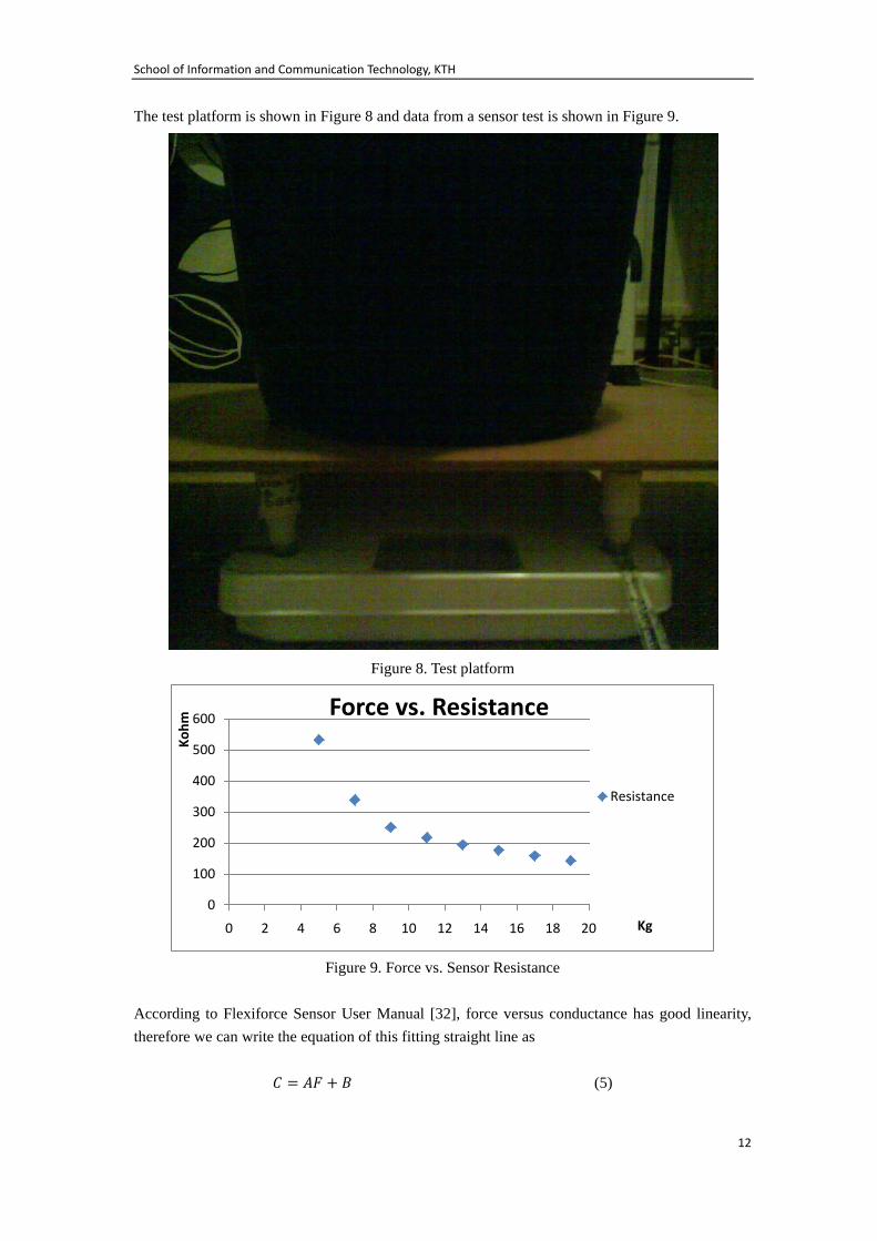
The test platform is shown in Figure 8 and data from a sensor test is shown in Figure 9.
Figure 8. Test platform
Figure 9. Force vs. Sensor Resistance
According to Flexiforce Sensor User Manual [32], force versus conductance has good linearity, therefore we can write the equation of this fitting straight line as
𝐶 = 𝐴𝐹 + 𝐵 (5)
0
100
200
300
400
500
600
0 2 4 6 8 10 12 14 16 18 20
Kohm
Kg
Force vs. Resistance
Resistance
School of Information and Communication Technology, KTH
13
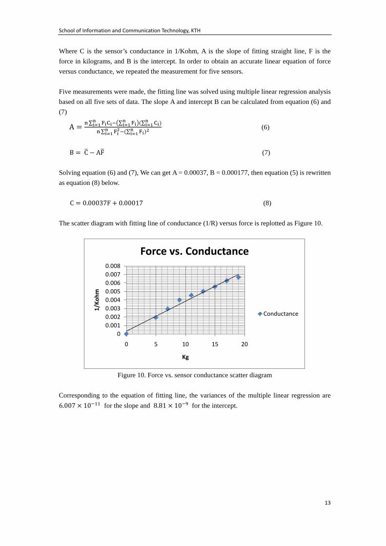
Where C is the sensor’s conductance in 1/Kohm, A is the slope of fitting straight line, F is the force in kilograms, and B is the intercept. In order to obtain an accurate linear equation of force versus conductance, we repeated the measurement for five sensors. Five measurements were made, the fitting line was solved using multiple linear regression analysis based on all five sets of data. The slope A and intercept B can be calculated from equation (6) and (7)
A = �∑ ������∑ ������ �(∑ ���
��� )�����∑ ��
��(∑ ������ )��
��� (6)
B = C� − AF� (7) Solving equation (6) and (7), We can get A = 0.00037, B = 0.000177, then equation (5) is rewritten as equation (8) below. C = 0.00037F + 0.00017 (8) The scatter diagram with fitting line of conductance (1/R) versus force is replotted as Figure 10.
Figure 10. Force vs. sensor conductance scatter diagram
Corresponding to the equation of fitting line, the variances of the multiple linear regression are 6.007 × 10��� for the slope and 8.81 × 10�� for the intercept.
00.0010.0020.0030.0040.0050.0060.0070.008
0 5 10 15 20
1/Ko
hm
Kg
Force vs. Conductance
Conductance
School of Information and Communication Technology, KTH
14
Chapter 4. System Design and
Implementation
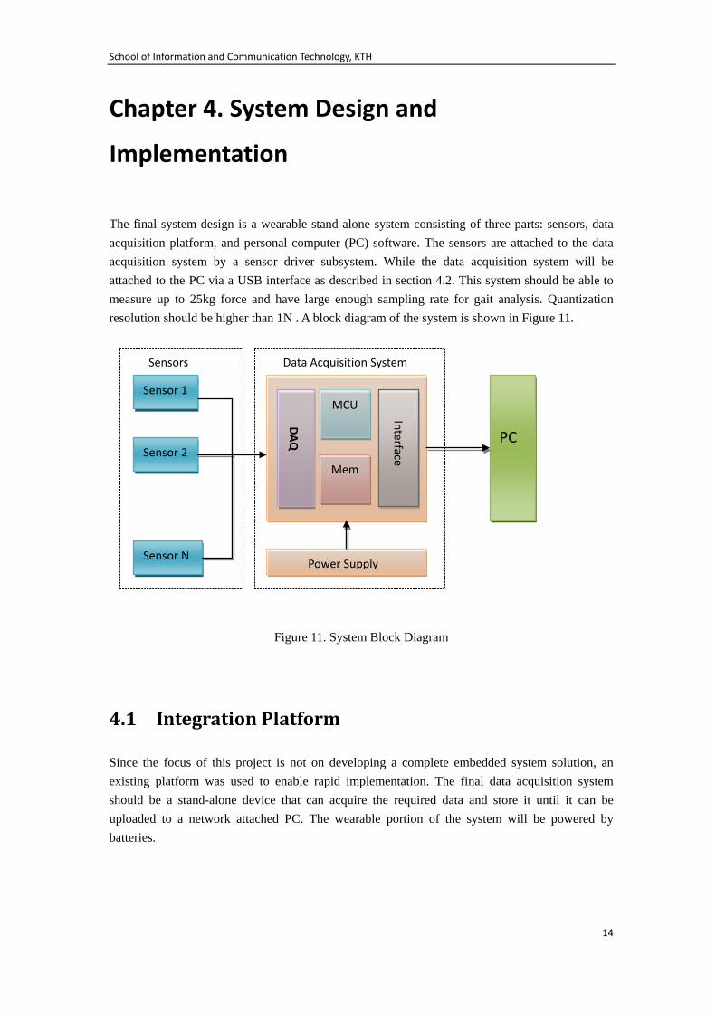
The final system design is a wearable stand-alone system consisting of three parts: sensors, data acquisition platform, and personal computer (PC) software. The sensors are attached to the data acquisition system by a sensor driver subsystem. While the data acquisition system will be attached to the PC via a USB interface as described in section 4.2. This system should be able to measure up to 25kg force and have large enough sampling rate for gait analysis. Quantization resolution should be higher than 1N . A block diagram of the system is shown in Figure 11.
Figure 11. System Block Diagram
4.1 Integration Platform
Since the focus of this project is not on developing a complete embedded system solution, an existing platform was used to enable rapid implementation. The final data acquisition system should be a stand-alone device that can acquire the required data and store it until it can be uploaded to a network attached PC. The wearable portion of the system will be powered by batteries.
Sensor 1
Sensor 2
Sensor N
DAQ
MCU
Mem
Interface
Power Supply
PC
Data Acquisition System Sensors
School of Information and Communication Technology, KTH
15
4.1.1 Platform Selection
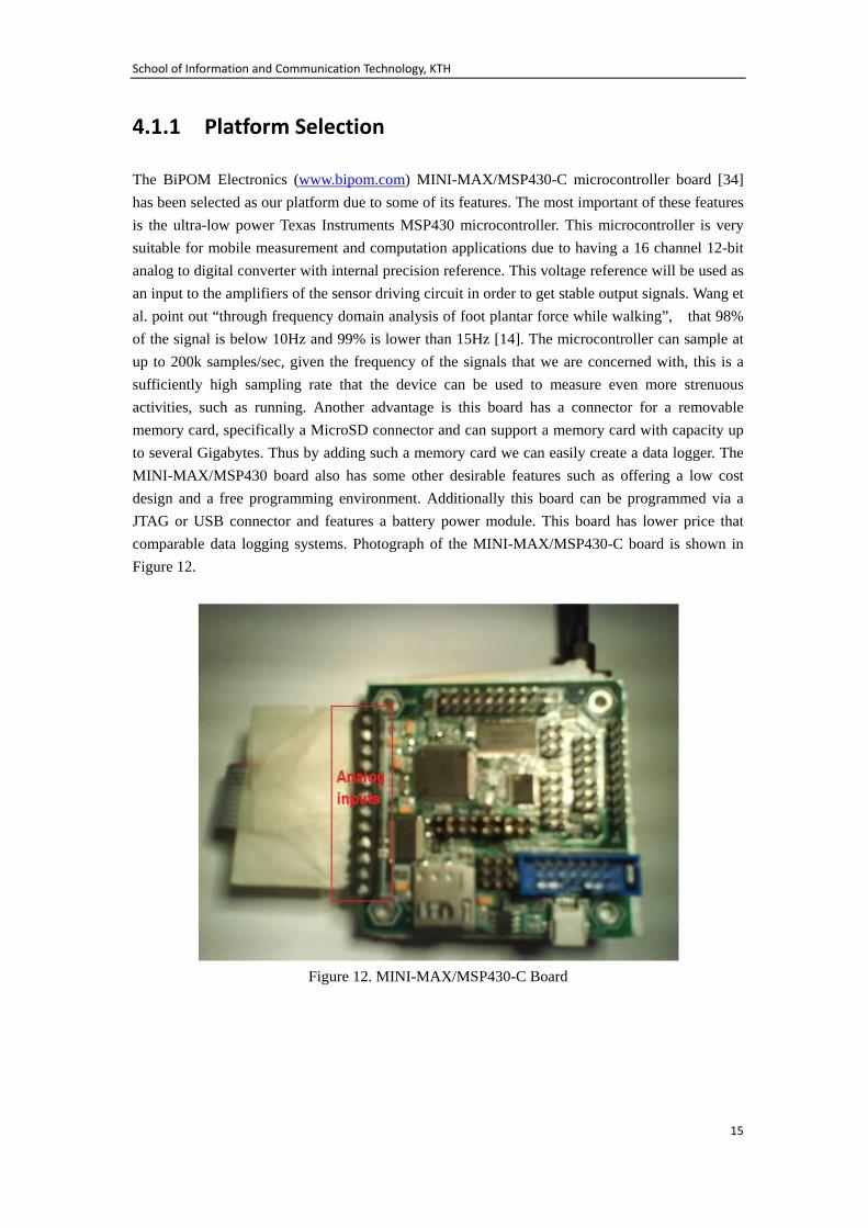
The BiPOM Electronics (www.bipom.com) MINI-MAX/MSP430-C microcontroller board [34] has been selected as our platform due to some of its features. The most important of these features is the ultra-low power Texas Instruments MSP430 microcontroller. This microcontroller is very suitable for mobile measurement and computation applications due to having a 16 channel 12-bit analog to digital converter with internal precision reference. This voltage reference will be used as an input to the amplifiers of the sensor driving circuit in order to get stable output signals. Wang et al. point out “through frequency domain analysis of foot plantar force while walking”, that 98% of the signal is below 10Hz and 99% is lower than 15Hz [14]. The microcontroller can sample at up to 200k samples/sec, given the frequency of the signals that we are concerned with, this is a sufficiently high sampling rate that the device can be used to measure even more strenuous activities, such as running. Another advantage is this board has a connector for a removable memory card, specifically a MicroSD connector and can support a memory card with capacity up to several Gigabytes. Thus by adding such a memory card we can easily create a data logger. The MINI-MAX/MSP430 board also has some other desirable features such as offering a low cost design and a free programming environment. Additionally this board can be programmed via a JTAG or USB connector and features a battery power module. This board has lower price that comparable data logging systems. Photograph of the MINI-MAX/MSP430-C board is shown in Figure 12.
Figure 12. MINI-MAX/MSP430-C Board

School of Information and Communication Technology, KTH
16
4.1.2 Microcontroller and Board Features
The features of the Texas Instruments MSP430F5437IPNR Ultra Low Power Microcontroller are shown in Table 4. The MINI-MAX/MSP430-C board complements the features of MSP430 processor by providing a USB connector, battery power module, external memory, JTAG programming interface, etc. The specification of the MINI-MAX/MSP430 board are shown in Table 5.
Table 4. Features of the Texas Instruments MSP430[34] Current consumption in Active Mode: 165 µA/MHz, Standby Mode: 2.60 µA 16 KB of on-chip static RAM and 256 KB of on-chip Flash for programs
16-bit RISC architecture Embedded Emulation Module (EEM) supports real-time in-system debugging
16 channel, 12-bit Analog to Digital Converter with internal precision reference
Low power Real-time clock with independent power and dedicated 32 kHz clock input. Dual serial port can be configured as UART, I2C, SPI or IrDA
One active mode and six software selectable low-power modes of operation
CPU operating voltage range: 2.2 V to 3.6 V
Table 5. MINI-MAX/MSP430-C Specification [34]
MINI-MAX/MSP430-C Board Specification
32.768 KHz crystal, with up to 18 MHz internal operation ( default is 1 MHz )
Ultra Low Power, USB or Battery operation possible, peripheral shutdown capability
Socket for MicroSD cards
Two RS232 Serial Ports with RTS/CTS handshake lines
USB Device port based on FTDI chipset JTAG programming interface
3.3 Volt on-board regulator Size: 5.97 cm x 6.10 cm
Working Temperature: 0 - 70° C
Storage Temperature: -40 - +85° C
Price: US$79
School of Information and Communication Technology, KTH
17
4.2 Hardware Implementation
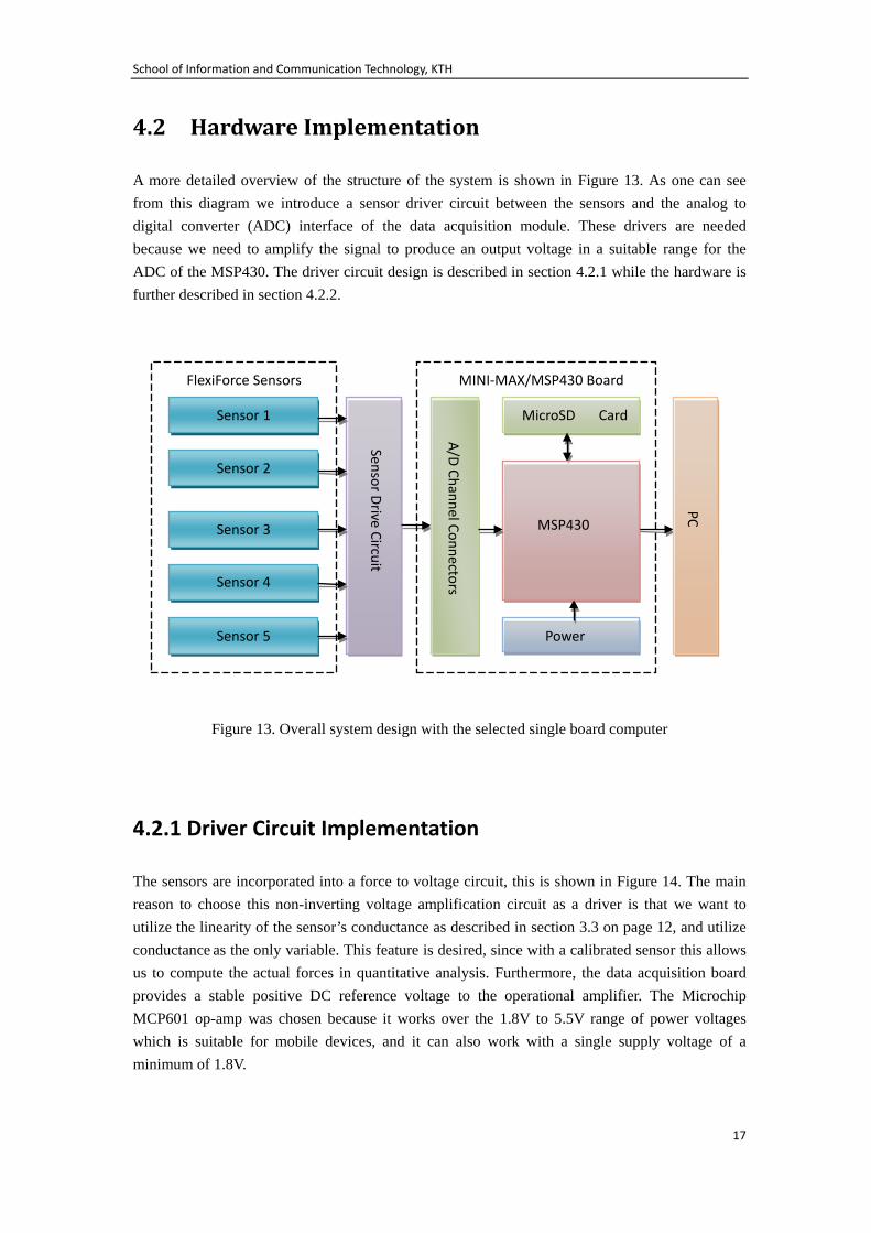
A more detailed overview of the structure of the system is shown in Figure 13. As one can see from this diagram we introduce a sensor driver circuit between the sensors and the analog to digital converter (ADC) interface of the data acquisition module. These drivers are needed because we need to amplify the signal to produce an output voltage in a suitable range for the ADC of the MSP430. The driver circuit design is described in section 4.2.1 while the hardware is further described in section 4.2.2.
Figure 13. Overall system design with the selected single board computer
4.2.1 Driver Circuit Implementation
The sensors are incorporated into a force to voltage circuit, this is shown in Figure 14. The main reason to choose this non-inverting voltage amplification circuit as a driver is that we want to utilize the linearity of the sensor’s conductance as described in section 3.3 on page 12, and utilize conductance as the only variable. This feature is desired, since with a calibrated sensor this allows us to compute the actual forces in quantitative analysis. Furthermore, the data acquisition board provides a stable positive DC reference voltage to the operational amplifier. The Microchip MCP601 op-amp was chosen because it works over the 1.8V to 5.5V range of power voltages which is suitable for mobile devices, and it can also work with a single supply voltage of a minimum of 1.8V.
Sensor 1
Sensor 2
Sensor 3
Sensor 5
Sensor Drive Circuit
MicroSD Card Reader
Power Supply
PC
A/D Channel Connectors
MSP430
MINI-MAX/MSP430 Board FlexiForce Sensors
Sensor 4
School of Information and Communication Technology, KTH
18
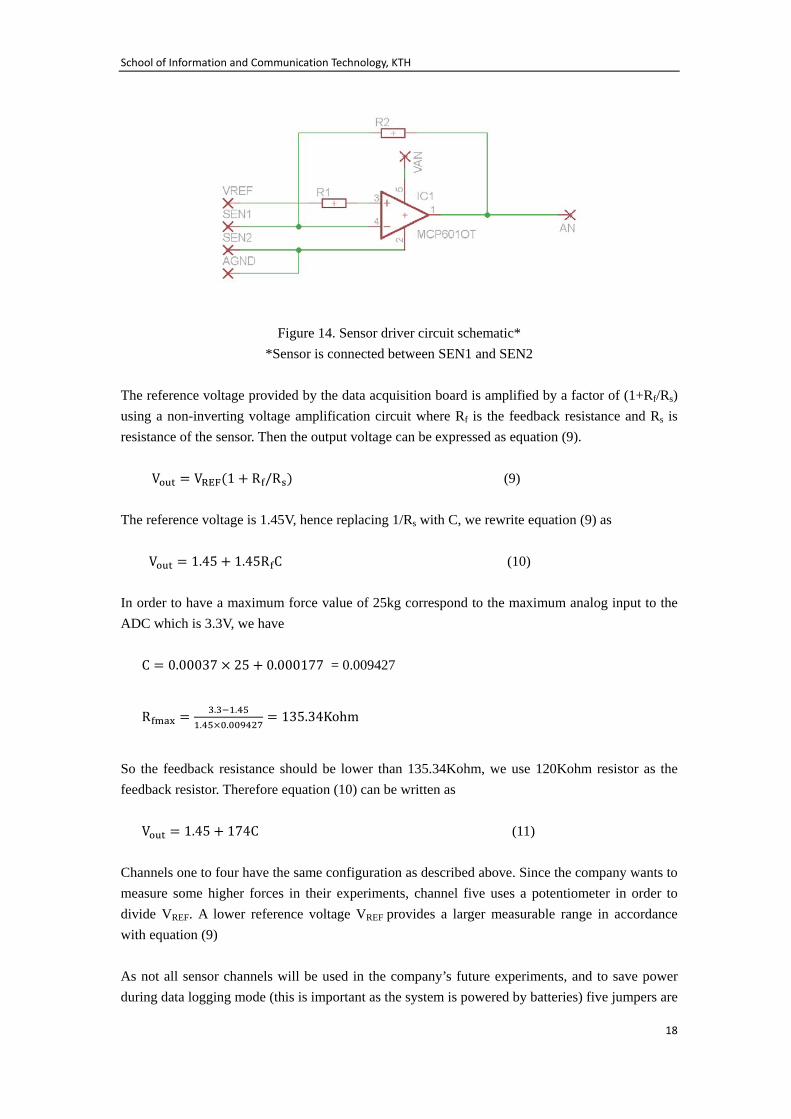
Figure 14. Sensor driver circuit schematic*
*Sensor is connected between SEN1 and SEN2 The reference voltage provided by the data acquisition board is amplified by a factor of (1+Rf/Rs) using a non-inverting voltage amplification circuit where Rf is the feedback resistance and Rs is resistance of the sensor. Then the output voltage can be expressed as equation (9). V��� = V���(1 + R�/R�) (9) The reference voltage is 1.45V, hence replacing 1/Rs with C, we rewrite equation (9) as V��� = 1.45 + 1.45R�C (10) In order to have a maximum force value of 25kg correspond to the maximum analog input to the ADC which is 3.3V, we have C = 0.00037 × 25 + 0.000177 = 0.009427
R���� = �.���.���.���.������
= 135.34Kohm
So the feedback resistance should be lower than 135.34Kohm, we use 120Kohm resistor as the feedback resistor. Therefore equation (10) can be written as V��� = 1.45 + 174C (11)
Channels one to four have the same configuration as described above. Since the company wants to measure some higher forces in their experiments, channel five uses a potentiometer in order to divide VREF. A lower reference voltage VREF provides a larger measurable range in accordance with equation (9) As not all sensor channels will be used in the company’s future experiments, and to save power during data logging mode (this is important as the system is powered by batteries) five jumpers are
School of Information and Communication Technology, KTH
19
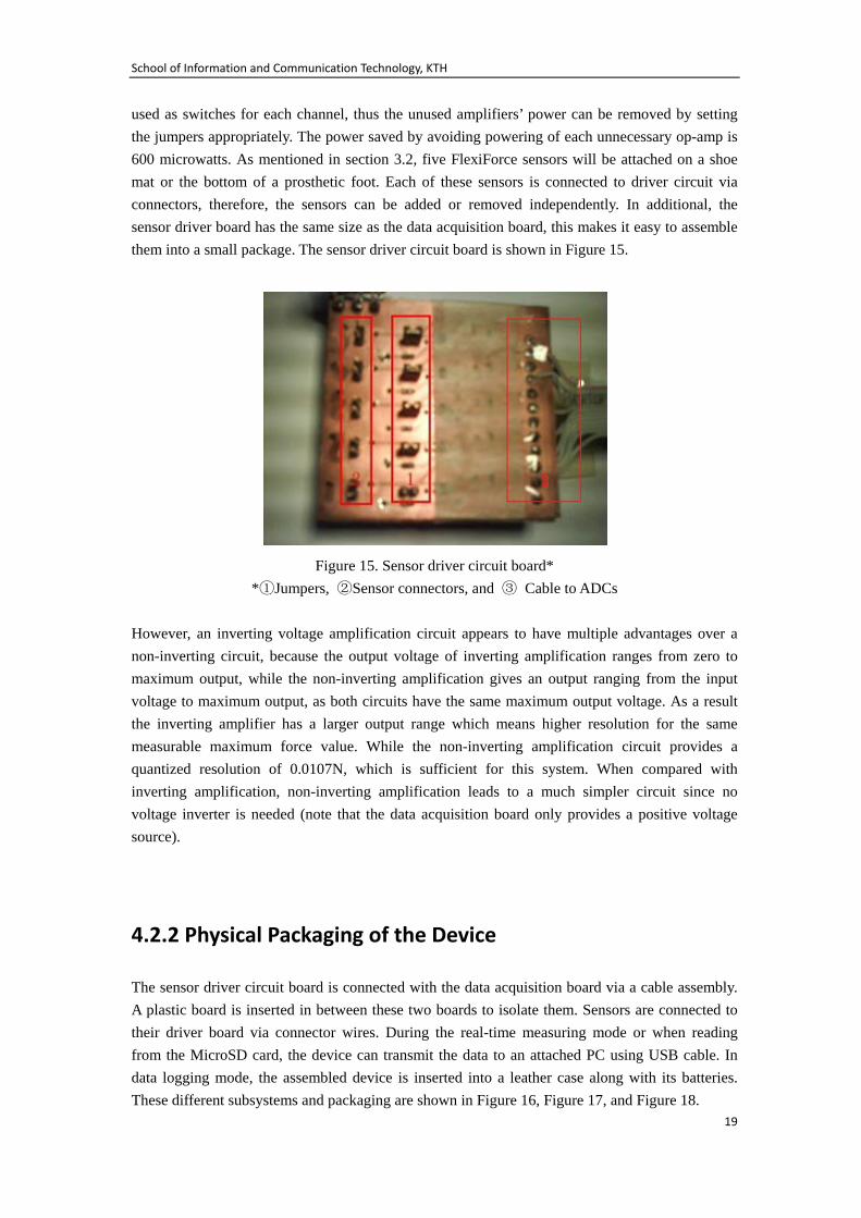
used as switches for each channel, thus the unused amplifiers’ power can be removed by setting the jumpers appropriately. The power saved by avoiding powering of each unnecessary op-amp is 600 microwatts. As mentioned in section 3.2, five FlexiForce sensors will be attached on a shoe mat or the bottom of a prosthetic foot. Each of these sensors is connected to driver circuit via connectors, therefore, the sensors can be added or removed independently. In additional, the sensor driver board has the same size as the data acquisition board, this makes it easy to assemble them into a small package. The sensor driver circuit board is shown in Figure 15.
Figure 15. Sensor driver circuit board* *①Jumpers, ②Sensor connectors, and ③ Cable to ADCs
However, an inverting voltage amplification circuit appears to have multiple advantages over a non-inverting circuit, because the output voltage of inverting amplification ranges from zero to maximum output, while the non-inverting amplification gives an output ranging from the input voltage to maximum output, as both circuits have the same maximum output voltage. As a result the inverting amplifier has a larger output range which means higher resolution for the same measurable maximum force value. While the non-inverting amplification circuit provides a quantized resolution of 0.0107N, which is sufficient for this system. When compared with inverting amplification, non-inverting amplification leads to a much simpler circuit since no voltage inverter is needed (note that the data acquisition board only provides a positive voltage source).
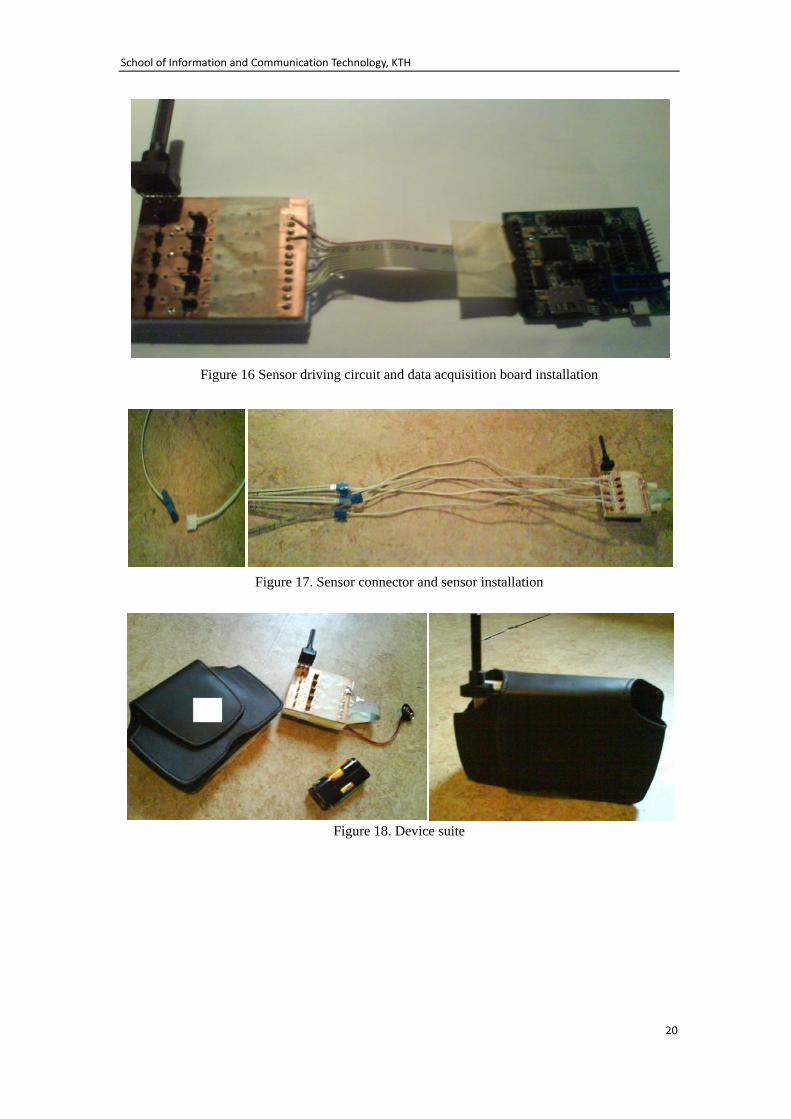
4.2.2 Physical Packaging of the Device
The sensor driver circuit board is connected with the data acquisition board via a cable assembly. A plastic board is inserted in between these two boards to isolate them. Sensors are connected to their driver board via connector wires. During the real-time measuring mode or when reading from the MicroSD card, the device can transmit the data to an attached PC using USB cable. In data logging mode, the assembled device is inserted into a leather case along with its batteries. These different subsystems and packaging are shown in Figure 16, Figure 17, and Figure 18.
School of Information and Communication Technology, KTH
20
Figure 16 Sensor driving circuit and data acquisition board installation
Figure 17. Sensor connector and sensor installation
Figure 18. Device suite
School of Information and Communication Technology, KTH
21
4.3 Device Fixture
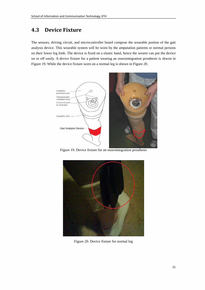
The sensors, driving circuit, and microcontroller board compose the wearable portion of the gait analysis device. This wearable system will be worn by the amputation patients or normal persons on their lower leg limb. The device is fixed on a elastic band, hence the wearer can put the device on or off easily. A device fixture for a patient wearing an osseointegration prosthesis is shwon in Figure 19. While the device fixture worn on a normal leg is shown in Figure 20.
Gait Analysis Device -
Figure 19. Device fixture for an osseointegration prosthesis
Figure 20. Device fixture for normal leg

School of Information and Communication Technology, KTH
22
4.4 Software Design
The software consists of two parts: data acquisition board software and PC application. As the ADC configuration directly influences other parts of data acquisition system design, it will be discussed in section 4.4.1, while PC application will be described in section 4.4.2.
4.4.1 ADC Configuration
We use the MSP430’s built-in analog to digital converter, which has been configured for 12-bit resolution. As a result, the resolution can be computed as follows: r = V���/4096 (12) Where Vmax is 3.3V. Therefore according to equation (11) the ADC result NADC can be calculated as N��� = 1.45/r + 174C/r = 1800 + 216000C (13) C = (N��� − 1800)/216000 (14) Then we introduce C from equation (14) to equation (8) (N��� − 1800)/216000 = 0.00037F + 0.00017 (15) Solve equation (15), the measuring force value F can be expressed as F = 0.01251N��� − 23 (16) F������� = 0.12271N��� − 225.55395 (17) Equation (17) is used to interpret the ADC result as the actual force value in Newtons. By using this setup, the maximum force can be measured is 277.1N. The ADC resolution in Newtons can be computed as
277.1/(4095-1800) = 0.12N (18) ADC module uses a sequence-of-channels mode and the USB serial port transmits data at the baud rate of 9600. So sample receiving rate for each ADC channel at PC side can be calculated as equation (19). Sample receiving rate = 9600/(8*13) = 92 samples/sec (19)* (*13-byte data frame is used, data format is described in section 4.5) Since in frequency domain, 99% plantar force signals are under 15Hz, the sampling rate should be larger than 30Hz. Hence a sampling rate of 92Hz is more than sufficient, and a low baud rate can save power.
School of Information and Communication Technology, KTH
23
4.4.2 PC Application
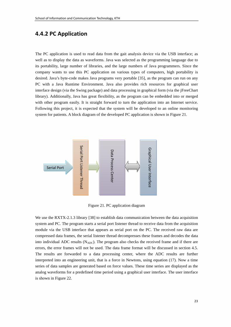
The PC application is used to read data from the gait analysis device via the USB interface; as well as to display the data as waveforms. Java was selected as the programming language due to its portability, large number of libraries, and the large numbers of Java programmers. Since the company wants to use this PC application on various types of computers, high portability is desired. Java’s byte-code makes Java programs very portable [35], as the program can run on any PC with a Java Runtime Environment. Java also provides rich resources for graphical user interface design (via the Swing package) and data processing in graphical form (via the jFreeChart library). Additionally, Java has great flexibility, as the program can be embedded into or merged with other program easily. It is straight forward to turn the application into an Internet service. Following this project, it is expected that the system will be developed to an online monitoring system for patients. A block diagram of the developed PC application is shown in Figure 21.
Figure 21. PC application diagram
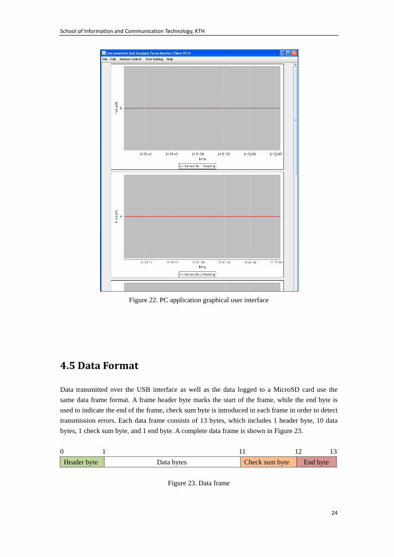
We use the RXTX-2.1.3 library [38] to establish data communication between the data acquisition system and PC. The program starts a serial port listener thread to receive data from the acquisition module via the USB interface that appears as serial port on the PC. The received raw data are compressed data frames, the serial listener thread decompresses these frames and decodes the data into individual ADC results (NADC). The program also checks the received frame and if there are errors, the error frames will not be used. The data frame format will be discussed in section 4.5. The results are forwarded to a data processing center, where the ADC results are further interpreted into an engineering unit, that is a force in Newtons, using equation (17). Now a time series of data samples are generated based on force values. These time series are displayed as the analog waveforms for a predefined time period using a graphical user interface. The user interface is shown in Figure 22.
Serial Port
Serial Port Listener Thread
Data Process Center
Graphical User Interface
School of Information and Communication Technology, KTH
24
Figure 22. PC application graphical user interface
4.5 Data Format
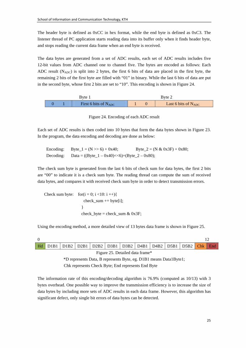
Data transmitted over the USB interface as well as the data logged to a MicroSD card use the same data frame format. A frame header byte marks the start of the frame, while the end byte is used to indicate the end of the frame, check sum byte is introduced in each frame in order to detect transmission errors. Each data frame consists of 13 bytes, which includes 1 header byte, 10 data bytes, 1 check sum byte, and 1 end byte. A complete data frame is shown in Figure 23. 0 1 11 12 13
Header byte Data bytes Check sum byte End byte
Figure 23. Data frame
School of Information and Communication Technology, KTH
25
The header byte is defined as 0xCC in hex format, while the end byte is defined as 0xC3. The listener thread of PC application starts reading data into its buffer only when it finds header byte, and stops reading the current data frame when an end byte is received. The data bytes are generated from a set of ADC results, each set of ADC results includes five 12-bit values from ADC channel one to channel five. The bytes are encoded as follows: Each ADC result (NADC) is split into 2 bytes, the first 6 bits of data are placed in the first byte, the remaining 2 bits of the first byte are filled with “01” in binary. While the last 6 bits of data are put in the second byte, whose first 2 bits are set to “10”. This encoding is shown in Figure 24. Byte 1 Byte 2
0 1 First 6 bits of NADC 1 0 Last 6 bits of NADC
Figure 24. Encoding of each ADC result Each set of ADC results is then coded into 10 bytes that form the data bytes shown in Figure 23. In the program, the data encoding and decoding are done as below:
Encoding: Byte_1 = (N >> 6) + 0x40; Byte_2 = (N & 0x3F) + 0x80; Decoding: Data = ((Byte_1 – 0x40)<<6)+(Byte_2 – 0x80);
The check sum byte is generated from the last 6 bits of check sum for data bytes, the first 2 bits are “00” to indicate it is a check sum byte. The reading thread can compute the sum of received data bytes, and compares it with received check sum byte in order to detect transmission errors.
Check sum byte: for(i = 0; i <10: i ++){ check_sum += byte[i];
} check_byte = check_sum & 0x3F;
Using the encoding method, a more detailed view of 13 bytes data frame is shown in Figure 25. 0 12 Hd D1B1 D1B2 D2B1 D2B2 D3B1 D3B2 D4B1 D4B2 D5B1 D5B2 Chk End
Figure 25. Detailed data frame* *D represents Data, B represents Byte, eg. D1B1 means Data1Byte1;
Chk represents Check Byte; End represents End Byte
The information rate of this encoding/decoding algorithm is 76.9% (computed as 10/13) with 3 bytes overhead. One possible way to improve the transmission efficiency is to increase the size of data bytes by including more sets of ADC results in each data frame. However, this algorithm has significant defect, only single bit errors of data bytes can be detected.
School of Information and Communication Technology, KTH
26
The data stored in MicroSD card used the same data format. Before the data frames were written into the card, they were accumulated to a data block with predefined size, it occurred when USB communication happened. When the data block was full, the whole block was written into MicroSD card once. Therefore the data logging rate equals to the USB transmission rate. The data were read out of the MicroSD card using the same transmission rate in order to have a sense of time.
4.6 System Test
Some tests were done on current version of prototype. Measurement tests were performed using known value forces applied on the scale platform, it provides early data related to the accuracy of this system. Power consumption tests gave relevant data for the operating time of this device.
4.6.1 Measurement Test
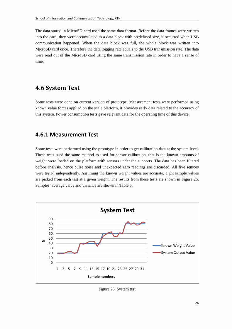
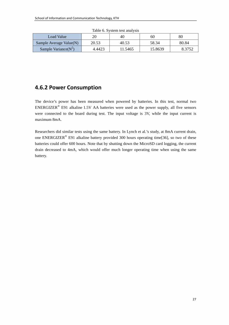
Some tests were performed using the prototype in order to get calibration data at the system level. These tests used the same method as used for sensor calibration, that is the known amounts of weight were loaded on the platform with sensors under the supports. The data has been filtered before analysis, hence pulse noise and unexpected zero readings are discarded. All five sensors were tested independently. Assuming the known weight values are accurate, eight sample values are picked from each test at a given weight. The results from these tests are shown in Figure 26. Samples’ average value and variance are shown in Table 6.
Figure 26. System test
0102030405060708090
1 3 5 7 9 11 13 15 17 19 21 23 25 27 29 31
N
Sample numbers
System Test
Known Weight Value
System Output Value
School of Information and Communication Technology, KTH
27
Table 6. System test analysis Load Value 20 40 60 80
Sample Average Value(N) 20.53 40.53 58.34 80.84 Sample Variance(N2) 4.4423 11.5465 15.8639 8.3752
4.6.2 Power Consumption
The device’s power has been measured when powered by batteries. In this test, normal two ENERGIZER® E91 alkaline 1.5V AA batteries were used as the power supply, all five sensors were connected to the board during test. The input voltage is 3V, while the input current is maximum 8mA. Researchers did similar tests using the same battery. In Lynch et al.’s study, at 8mA current drain, one ENERGIZER® E91 alkaline battery provided 300 hours operating time[36], so two of these batteries could offer 600 hours. Note that by shutting down the MicroSD card logging, the current drain decreased to 4mA, which would offer much longer operating time when using the same battery.
School of Information and Communication Technology, KTH
28
Chapter 5. Trials
The goal of this thesis project was to provide a system to do gait analysis. To avoid overloading or underloading during rehabilitation process of amputation, the peak force data are important. As a result, the research will focus on collecting and analyzing peak force values at five sensing points: Heel, Meta Tarsal Head 1, Meta Tarsal Head 3, Meta Tarsal Head 5, and Toe under different gait states.
5.1 Methods
Before the system is used by amputation patients, the research was conducted on a normal leg. As an initial study, the data of a normal person’s gait can be used as a sample of a larger future control group. The author acted as the first normal volunteer for a study sample for this research. The relevant physical data of author is shown in Table 7.
Table 7. Relevant sample physical condition Gender Male Height 173cm Weight 63kg
Right Foot Sole Maximum Length 24cm Right Foot Sole Maximum Width 9.5cm
Different genders may have different gait paces as well as foot dropping velocities, which can affect the force value applied on the contact surface between foot sole and ground. The height of the person can affect their gravity center changing the measuring results during gait movement. The person’s weight directly influences the measurement. Detail of the foot determines the actual positions of sensors’ attachments. Using body mass index (BMI) as indicator , the author has BMI of 21.0, which is within the normal range. In this research, the sensors are fixed to shoe mat suitably for the author’s right foot. Placement of the sensors is shown later in Figure 27 on page 27. During the trial, the stand still state will be measured first. The force value for each sensing point will be recorded, these results can be used as control group for further dynamic measurements. Next, some trials while in a straight walking state will be conducted, after which turning and jumping states will be studied. All of these trials were done on flat ground. The device was set to data logging mode and the data recorded in the MicroSD card. After transferring this data to the PC, the collected data were displayed as waveforms by using the PC application, and log files generated on the PC for the further analysis in Chapter 6. The trials and results will be discussed and compared with former works in this area in order to address limitations and problems.

School of Information and Communication Technology, KTH
29
5.2 Trial of Standing State
The sensors are attached to the shoe as shown in Figure 27. In the standing state, the study object is required to stand vertically with both feet together, and remain still for several minutes in order to obtain stable data sets. The measurement configuration during this trial is shown in Figure 28. Note that to improve the contact between sensing area and shoe, a metal puck was attached to each of the sensors’ sensing points. The puck has a diameter of 0.8mm which is slightly smaller than sensing area (diameter of 9.53mm). The pucks are made of aluminum with thickness of approximately 0.3mm.
Figure 27. Sensor attachment for trials*
*① Toe, ② Meta Tarsal Head 1, ③ Meta Tarsal Head 3, ④ Meta Tarsal Head 5, ⑤ Heel
Figure 28. Standing state trial
School of Information and Communication Technology, KTH
30
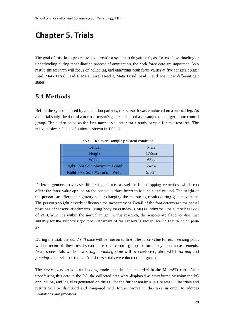
The measured force values for the five sensing points are read from the MicroSD card by the PC application, and the data displayed as waveforms. A view of all of these waveforms from a single trial is shown in Figure 29. Y-axis shows force values in Newtons.
Figure 29. Waveforms of standing trial
6.3 Dynamic Trials
In gait trials, straight slow walking state, turning state, and jumping state of study object will be measured.
5.3.1 Straight Walking Trial
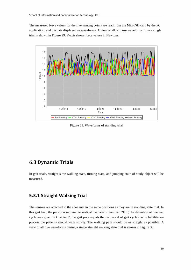
The sensors are attached to the shoe mat in the same positions as they are in standing state trial. In this gait trial, the person is required to walk at the pace of less than 2Hz (The definition of one gait cycle was given in Chapter 2, the gait pace equals the reciprocal of gait cycle), as in habilitation process the patients should walk slowly. The walking path should be as straight as possible. A view of all five waveforms during a single straight walking state trial is shown in Figure 30.
School of Information and Communication Technology, KTH
31
Figure 30. Waveforms of straight walking trial
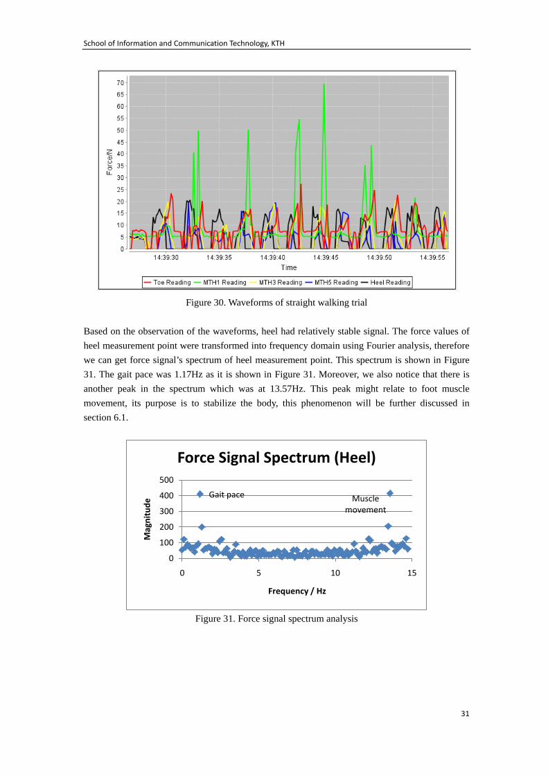
Based on the observation of the waveforms, heel had relatively stable signal. The force values of heel measurement point were transformed into frequency domain using Fourier analysis, therefore we can get force signal’s spectrum of heel measurement point. This spectrum is shown in Figure 31. The gait pace was 1.17Hz as it is shown in Figure 31. Moreover, we also notice that there is another peak in the spectrum which was at 13.57Hz. This peak might relate to foot muscle movement, its purpose is to stabilize the body, this phenomenon will be further discussed in section 6.1.
Figure 31. Force signal spectrum analysis
Gait pace Muscle movement
0
100
200
300
400
500
0 5 10 15
Mag
nitu
de
Frequency / Hz
Force Signal Spectrum (Heel)
School of Information and Communication Technology, KTH
32
5.3.2 Turning Trial
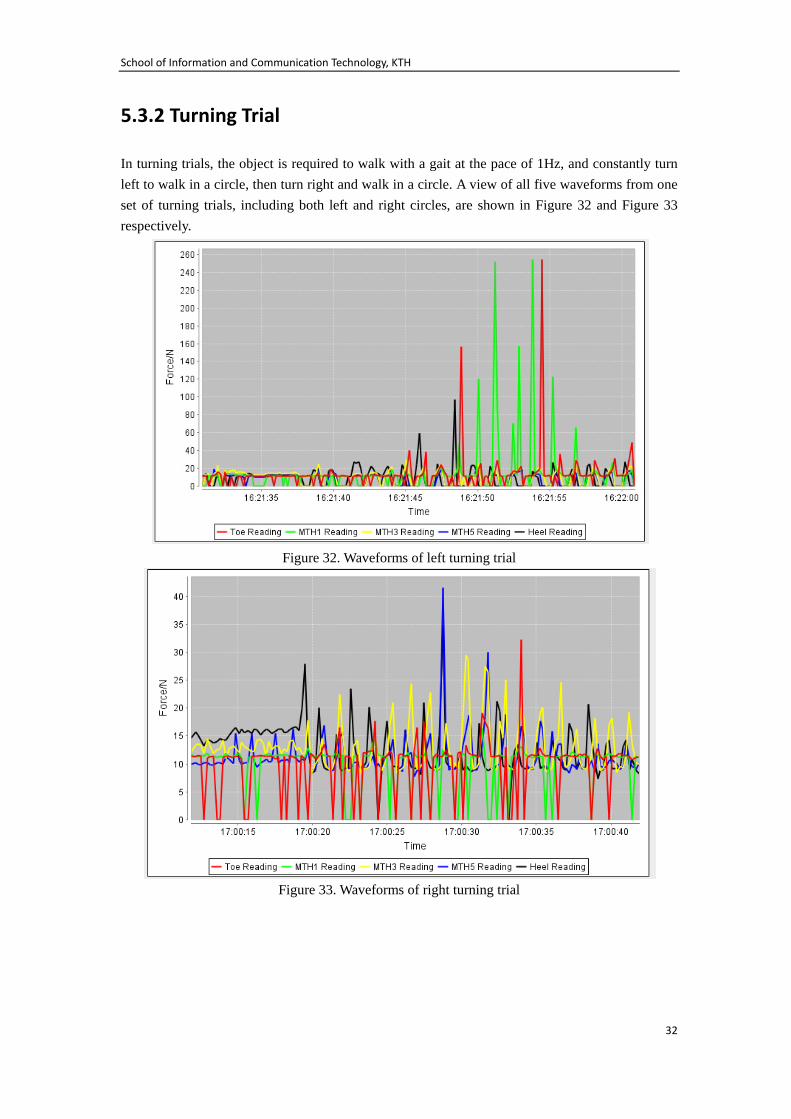
In turning trials, the object is required to walk with a gait at the pace of 1Hz, and constantly turn left to walk in a circle, then turn right and walk in a circle. A view of all five waveforms from one set of turning trials, including both left and right circles, are shown in Figure 32 and Figure 33 respectively.
Figure 32. Waveforms of left turning trial
Figure 33. Waveforms of right turning trial

School of Information and Communication Technology, KTH
33
5.3.3 Jumping Trial
In jumping trials, the suject stays at the same spot and jumps approximately 5 cm up or down. In the first phase of trial, the forefoot contacts the ground before the hind foot does during dropping, while in second phase the whole foot contacts the ground nearly at the same time. The waveforms in Figure 34 shows both phases in one of these trials.
Figure 34. Waveforms of jumping trial*
*① Forefoot contacting first ② Whole foot contacting
School of Information and Communication Technology, KTH
34
Chapter 6. Analysis and Results
Based on the different types of trials introduced in last chapter, the trial results are shown and analyzed in this chapter. Key factors such as average values, variance, and peak values are examined.
6.1 Standing State Analysis
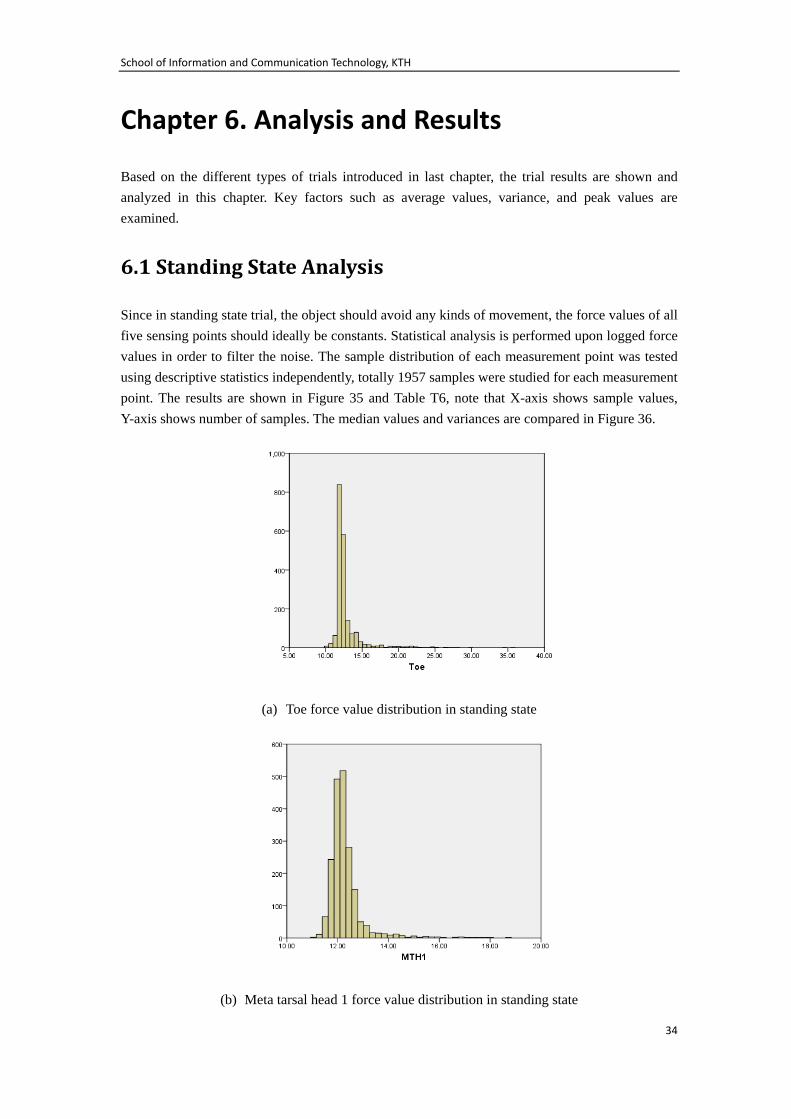
Since in standing state trial, the object should avoid any kinds of movement, the force values of all five sensing points should ideally be constants. Statistical analysis is performed upon logged force values in order to filter the noise. The sample distribution of each measurement point was tested using descriptive statistics independently, totally 1957 samples were studied for each measurement point. The results are shown in Figure 35 and Table T6, note that X-axis shows sample values, Y-axis shows number of samples. The median values and variances are compared in Figure 36.
(a) Toe force value distribution in standing state
(b) Meta tarsal head 1 force value distribution in standing state
School of Information and Communication Technology, KTH
35
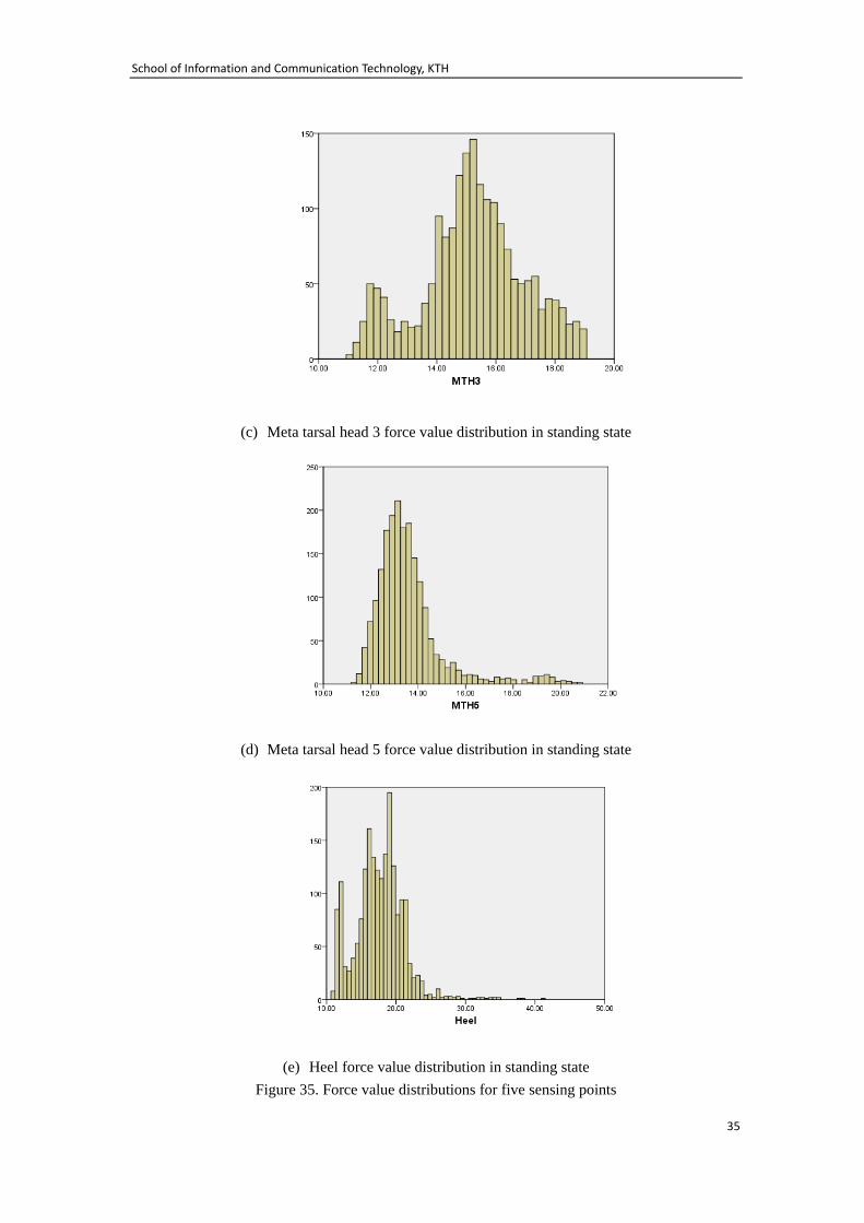
(c) Meta tarsal head 3 force value distribution in standing state
(d) Meta tarsal head 5 force value distribution in standing state
(e) Heel force value distribution in standing state
Figure 35. Force value distributions for five sensing points
School of Information and Communication Technology, KTH
36
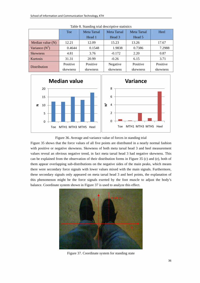
Table 8. Standing trial descriptive statistics Toe Meta Tarsal
Head 1 Meta Tarsal
Head 3 Meta Tarsal
Head 5 Heel
Median value (N) 12.21 12.09 15.23 13.26 17.67 Variance (N2) 0.4644 0.1548 1.9838 0.7386 7.2988 Skewness 4.81 3.76 -0.172 2.20 0.87 Kurtosis 31.31 20.99 -0.26 6.15 3.71
Distribution Positive
skewness Positive
skewness Negative skewness
Positive skewness
Positive skewness
Figure 36. Average and variance value of forces in standing trial Figure 35 shows that the force values of all five points are distributed in a nearly normal fashion with positive or negative skewness. Skewness of both meta tarsal head 3 and heel measurement values reveal an obvious negative trend, in fact meta tarsal head 3 had negative skewness. This can be explained from the observation of their distribution forms in Figure 35 (c) and (e), both of them appear overlapping sub-distributions on the negative sides of the main peaks, which means there were secondary force signals with lower values mixed with the main signals. Furthermore, these secondary signals only appeared on meta tarsal head 3 and heel points, the explanation of this phenomenon might be the force signals exerted by the foot muscle to adjust the body’s balance. Coordinate system shown in Figure 37 is used to analyze this effect.
Figure 37. Coordinate system for standing state
0
5
10
15
20
Toe MTH1 MTH3 MTH5 Heel
N
Median value
0
2
4
6
8
Toe MTH1 MTH3 MTH5 Heel
N2
Variance
X
Y Middle line
School of Information and Communication Technology, KTH
37
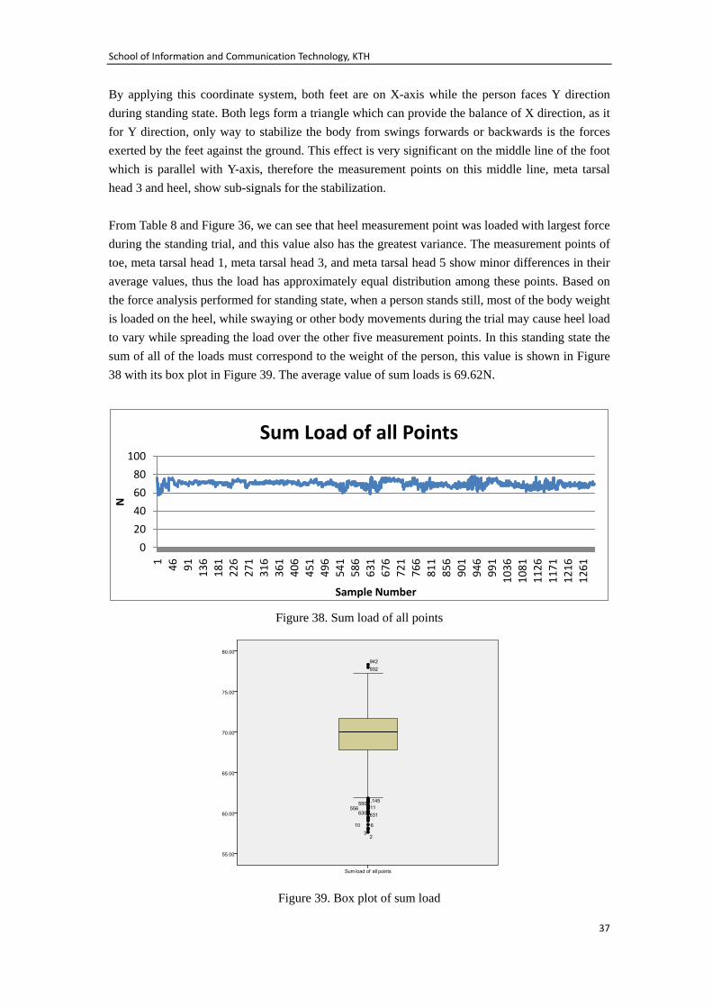
By applying this coordinate system, both feet are on X-axis while the person faces Y direction during standing state. Both legs form a triangle which can provide the balance of X direction, as it for Y direction, only way to stabilize the body from swings forwards or backwards is the forces exerted by the feet against the ground. This effect is very significant on the middle line of the foot which is parallel with Y-axis, therefore the measurement points on this middle line, meta tarsal head 3 and heel, show sub-signals for the stabilization. From Table 8 and Figure 36, we can see that heel measurement point was loaded with largest force during the standing trial, and this value also has the greatest variance. The measurement points of toe, meta tarsal head 1, meta tarsal head 3, and meta tarsal head 5 show minor differences in their average values, thus the load has approximately equal distribution among these points. Based on the force analysis performed for standing state, when a person stands still, most of the body weight is loaded on the heel, while swaying or other body movements during the trial may cause heel load to vary while spreading the load over the other five measurement points. In this standing state the sum of all of the loads must correspond to the weight of the person, this value is shown in Figure 38 with its box plot in Figure 39. The average value of sum loads is 69.62N.
Figure 38. Sum load of all points
Figure 39. Box plot of sum load
020406080
100
1 46 91 136
181
226
271
316
361
406
451
496
541
586
631
676
721
766
811
856
901
946
991
1036
1081
1126
1171
1216
1261
N
Sample Number
Sum Load of all Points
School of Information and Communication Technology, KTH
38
It can be observed from the box plot that the distances from the median value to both lower and upper quartiles are roughly equal, so to smallest observation and the largest observation. This means the body was trying to balance itself during the standing state, when the body swung towards certain direction, the measurement points on that direction took higher loads, ones on the contrary direction took lower loads, then the body bounced back. The sum of all points should be generally maintain a constant, the median value of sum loads is 70.00N.
6.2 Dynamic Gait Analysis
In this section, trials in which human movements are involved, such as straight walking state, turning walking state as well as jumping state, will be discussed.
6.2.1 Straight Walking Analysis
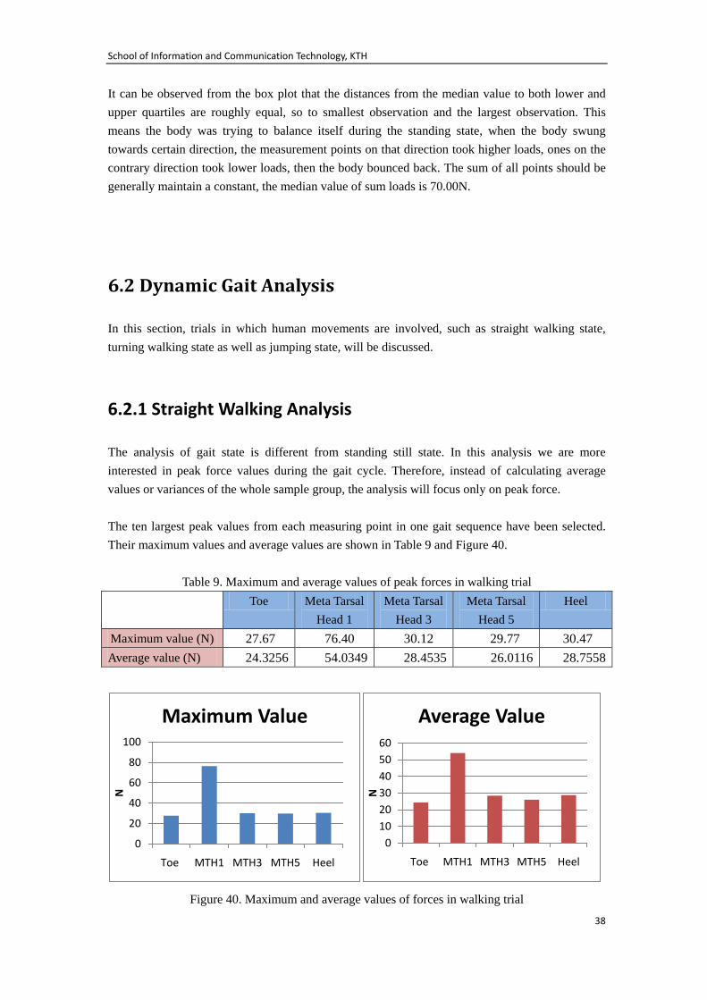
The analysis of gait state is different from standing still state. In this analysis we are more interested in peak force values during the gait cycle. Therefore, instead of calculating average values or variances of the whole sample group, the analysis will focus only on peak force. The ten largest peak values from each measuring point in one gait sequence have been selected. Their maximum values and average values are shown in Table 9 and Figure 40.
Table 9. Maximum and average values of peak forces in walking trial Toe Meta Tarsal
Head 1 Meta Tarsal
Head 3 Meta Tarsal
Head 5 Heel
Maximum value (N) 27.67 76.40 30.12 29.77 30.47 Average value (N) 24.3256 54.0349 28.4535 26.0116 28.7558
Figure 40. Maximum and average values of forces in walking trial
0
20
40
60
80
100
Toe MTH1 MTH3 MTH5 Heel
N
Maximum Value
0102030405060
Toe MTH1 MTH3 MTH5 Heel
N
Average Value
School of Information and Communication Technology, KTH
39
Comparing with standing state, all measurement points appear to have higher loads during walking. The load applied on the toe is 12N higher than in standing state, 41.9N higher for meta tarsal head 1, 13.8N higher for meta tarsal head 3, 12.8N higher for meta tarsal head 5, and 11.5N higher for the heel respectively. Meta tarsal head 1 also shows largest change from standing state, this indicates that the person may use the area of tarsal head 1 to push back when stepping forward. Dropping on the ground causes greater loads than in the standing trial for all five points. Note that dropping forces include both the force due the weight of the person and the their acceleration under gravity downward.
6.2.2 Turning Analysis
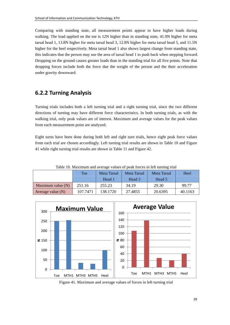
Turning trials includes both a left turning trial and a right turning trial, since the two different directions of turning may have different force characteristics. In both turning trials, as with the walking trial, only peak values are of interest. Maximum and average values for the peak values from each measurement point are analyzed. Eight turns have been done during both left and right turn trials, hence eight peak force values from each trial are chosen accordingly. Left turning trial results are shown in Table 10 and Figure 41 while right turning trial results are shown in Table 11 and Figure 42.
Table 10. Maximum and average values of peak forces in left turning trial Toe Meta Tarsal
Head 1 Meta Tarsal
Head 3 Meta Tarsal
Head 5 Heel
Maximum value (N) 251.16 255.23 34.19 29.30 99.77 Average value (N) 107.7471 138.1720 27.4855 20.6395 40.1163
Figure 41. Maximum and average values of forces in left turning trial
0
50
100
150
200
250
300
Toe MTH1 MTH3 MTH5 Heel
N
Maximum Value
0
20
40
60
80
100
120
140
160
Toe MTH1 MTH3 MTH5 Heel
N
Average Value
School of Information and Communication Technology, KTH
40
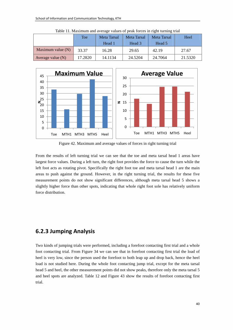
Table 11. Maximum and average values of peak forces in right turning trial Toe Meta Tarsal
Head 1 Meta Tarsal
Head 3 Meta Tarsal
Head 5 Heel
Maximum value (N) 33.37 16.28 29.65 42.19 27.67
Average value (N) 17.2820 14.1134 24.5204 24.7064 21.5320
Figure 42. Maximum and average values of forces in right turning trial
From the results of left turning trial we can see that the toe and meta tarsal head 1 areas have largest force values. During a left turn, the right foot provides the force to cause the turn while the left foot acts as rotating pivot. Specifically the right foot toe and meta tarsal head 1 are the main areas to push against the ground. However, in the right turning trial, the results for these five measurement points do not show significant differences, although meta tarsal head 5 shows a slightly higher force than other spots, indicating that whole right foot sole has relatively uniform force distribution.
6.2.3 Jumping Analysis
Two kinds of jumping trials were performed, including a forefoot contacting first trial and a whole foot contacting trial. From Figure 34 we can see that in forefoot contacting first trial the load of heel is very low, since the person used the forefoot to both leap up and drop back, hence the heel load is not studied here. During the whole foot contacting jump trial, except for the meta tarsal head 5 and heel, the other measurement points did not show peaks, therefore only the meta tarsal 5 and heel spots are analyzed. Table 12 and Figure 43 show the results of forefoot contacting first trial.
05
1015202530354045
Toe MTH1 MTH3 MTH5 Heel
N
Maximum Value
0
5
10
15
20
25
30
Toe MTH1 MTH3 MTH5 Heel
N
Average Value
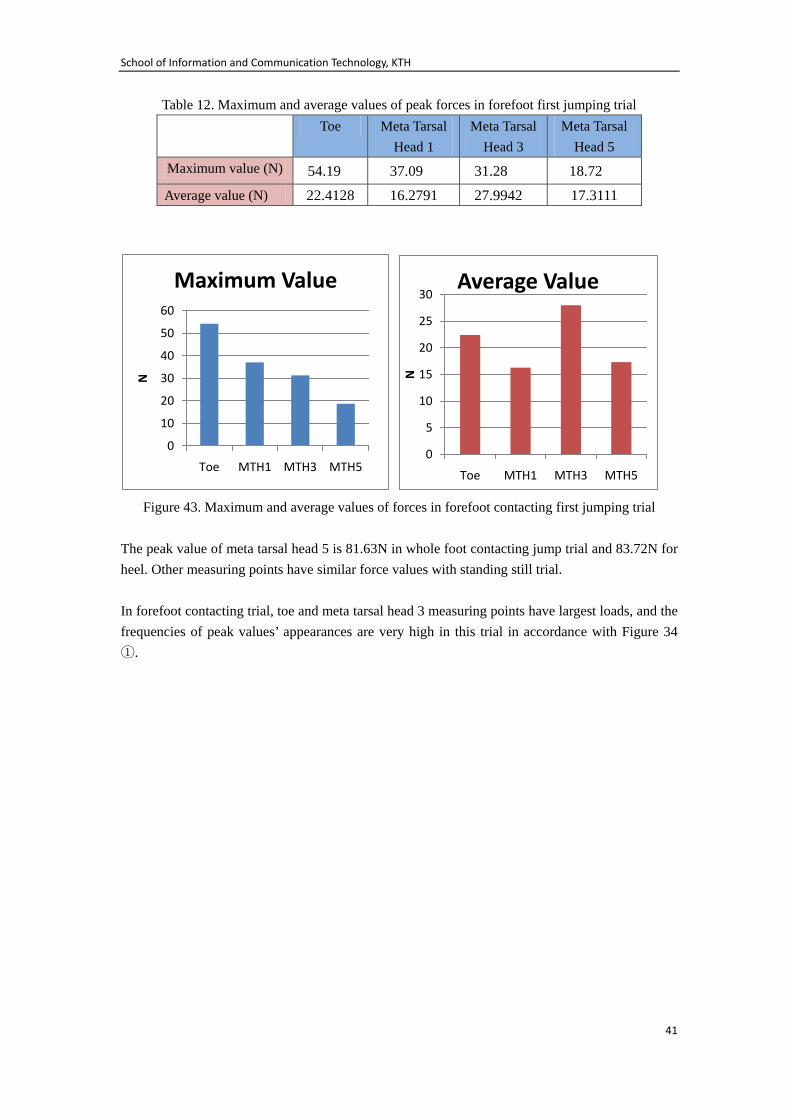
School of Information and Communication Technology, KTH
41
Table 12. Maximum and average values of peak forces in forefoot first jumping trial Toe Meta Tarsal
Head 1 Meta Tarsal
Head 3 Meta Tarsal
Head 5 Maximum value (N) 54.19 37.09 31.28 18.72
Average value (N) 22.4128 16.2791 27.9942 17.3111
Figure 43. Maximum and average values of forces in forefoot contacting first jumping trial
The peak value of meta tarsal head 5 is 81.63N in whole foot contacting jump trial and 83.72N for heel. Other measuring points have similar force values with standing still trial. In forefoot contacting trial, toe and meta tarsal head 3 measuring points have largest loads, and the frequencies of peak values’ appearances are very high in this trial in accordance with Figure 34 ①.
0
10
20
30
40
50
60
Toe MTH1 MTH3 MTH5
N
Maximum Value
0
5
10
15
20
25
30
Toe MTH1 MTH3 MTH5
N
Average Value
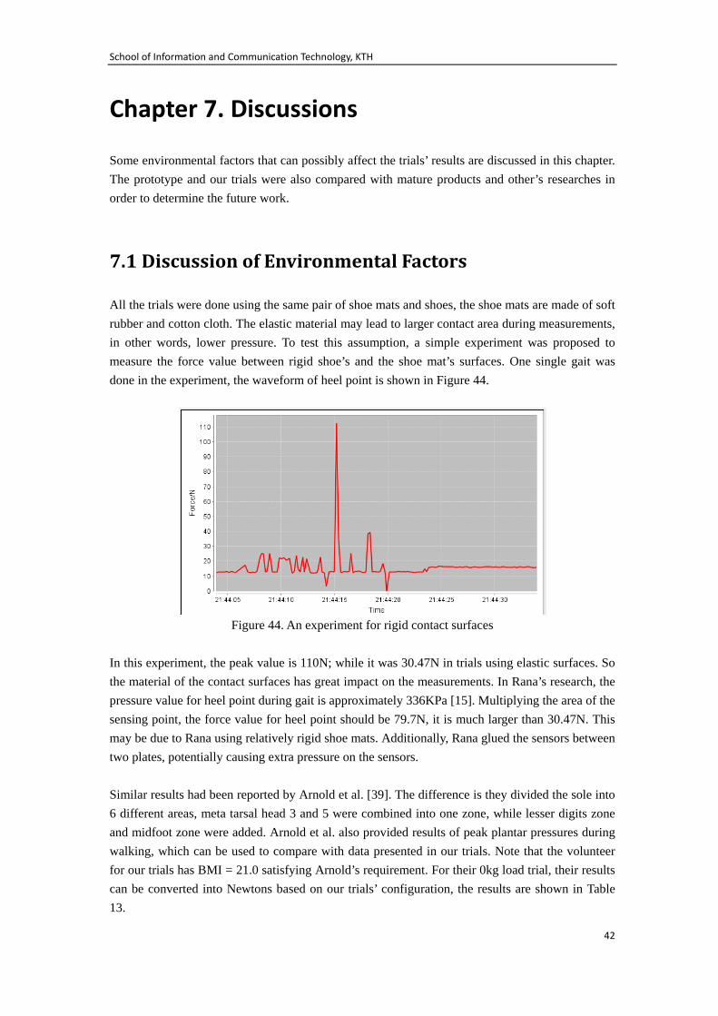
School of Information and Communication Technology, KTH
42
Chapter 7. Discussions
Some environmental factors that can possibly affect the trials’ results are discussed in this chapter. The prototype and our trials were also compared with mature products and other’s researches in order to determine the future work.
7.1 Discussion of Environmental Factors
All the trials were done using the same pair of shoe mats and shoes, the shoe mats are made of soft rubber and cotton cloth. The elastic material may lead to larger contact area during measurements, in other words, lower pressure. To test this assumption, a simple experiment was proposed to measure the force value between rigid shoe’s and the shoe mat’s surfaces. One single gait was done in the experiment, the waveform of heel point is shown in Figure 44.
Figure 44. An experiment for rigid contact surfaces
In this experiment, the peak value is 110N; while it was 30.47N in trials using elastic surfaces. So the material of the contact surfaces has great impact on the measurements. In Rana’s research, the pressure value for heel point during gait is approximately 336KPa [15]. Multiplying the area of the sensing point, the force value for heel point should be 79.7N, it is much larger than 30.47N. This may be due to Rana using relatively rigid shoe mats. Additionally, Rana glued the sensors between two plates, potentially causing extra pressure on the sensors. Similar results had been reported by Arnold et al. [39]. The difference is they divided the sole into 6 different areas, meta tarsal head 3 and 5 were combined into one zone, while lesser digits zone and midfoot zone were added. Arnold et al. also provided results of peak plantar pressures during walking, which can be used to compare with data presented in our trials. Note that the volunteer for our trials has BMI = 21.0 satisfying Arnold’s requirement. For their 0kg load trial, their results can be converted into Newtons based on our trials’ configuration, the results are shown in Table 13.
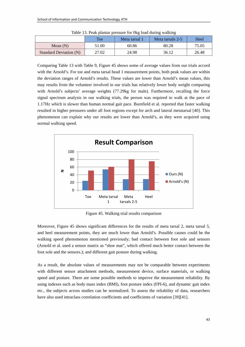
School of Information and Communication Technology, KTH
43
Table 13. Peak plantar pressure for 0kg load during walking Toe Meta tarsal 1 Meta tarsals 2-5 Heel
Mean (N) 51.00 60.86 80.28 75.05 Standard Deviation (N) 27.02 24.98 36.12 26.48
Comparing Table 13 with Table 9, Figure 45 shows some of average values from our trials accord with the Arnold’s. For toe and meta tarsal head 1 measurement points, both peak values are within the deviation ranges of Arnold’s results. These values are lower than Arnold’s mean values, this may results from the volunteer involved in our trials has relatively lower body weight comparing with Arnold’s subjects’ average weights (77.29kg for male). Furthermore, recalling the force signal spectrum analysis in our walking trials, the person was required to walk at the pace of 1.17Hz which is slower than human normal gait pace. Burnfield et al. reported that faster walking resulted in higher pressures under all foot regions except for arch and lateral metatarsal [40]. This phenomenon can explain why our results are lower than Arnold’s, as they were acquired using normal walking speed.
Figure 45. Walking trial results comparison
Moreover, Figure 45 shows significant differences for the results of meta tarsal 2, meta tarsal 5, and heel measurement points, they are much lower than Arnold’s. Possible causes could be the walking speed phenomenon mentioned previously; bad contact between foot sole and sensors (Arnold et al. used a sensor matrix as “shoe mat”, which offered much better contact between the foot sole and the sensors.); and different gait posture during walking. As a result, the absolute values of measurements may not be comparable between experiments with different sensor attachment methods, measurement device, surface materials, or walking speed and posture. There are some possible methods to improve the measurement reliability. By using indexes such as body mass index (BMI), foot posture index (FPI-6), and dynamic gait index etc., the subjects across studies can be normalized. To assess the reliability of data, researchers have also used intraclass correlation coefficients and coefficients of variation [39][41].
0
20
40
60
80
100
Toe Meta tarsal 1
Meta tarsals 2-5
Heel
N
Result Comparison
Ours (N)
Arnold's (N)

School of Information and Communication Technology, KTH
44
7.2 Comparison
In this section, our prototype and trials will be compared with several gait analysis instruments and other’s researches. The extensive studies can also help determine possible future development.
7.2.1 F-Scan® System Applications
The system Arnold et al. used in their research was F-Scan® System in-shoe plantar pressure analysis system (Tekscan, Inc., USA). There are some beneficial features offered by F-Scan® system. It utilizes a sensor matrix instead of single force sensor, the F-Scan® sensor is extremely thin, and highly sensitive[31]. The resolution is 50-75 Pascals, calculating with the sensing area used in our research, it offers 0.021N resolution in Newtons corresponding to our sensing area. Moreover, the sensor can be trimmed to fit various shoe sizes. For its software, it can display dynamic 2-D and 3-D forces in real time, force versus time curves can be generated. Different areas of sensor matrix can be separated to enable single zone analysis. Based on the literature review on plantar force analysis, F-Scan® system is one of the most popular devices that hasbeen used by researchers in this area, its reliability has also been explicitly and repeatedly tested. Regarding normal gait analysis, Young[42] and Mueller & Strube [43] used the F-Scan® system to investigate in-shoe pressure distribution or peak pressure for the normal person; Frykberg et al.[44] and Pitei et al.[45] performed studies on in-shoe pressures of diabetic foot using this system; researchers also used F-Scan® system to support orthotic design, such as Nowak et al.[46]. To sum up, the F-Scan® system has been widely used in plantar force analysis applications, it has significant advantages over our developed system regarding measurement accuracy, repeatability, data processing, etc. However, it was also reported that F-Scan® system lacks durability and suffers significant calibration error [47]. Based on Tekscan’s website, the data logging function of F-Scan® system are still under development, while our prototype can already store measurement data in a portable memory card. Meanwhile, F-Scan® system is extremely expensive compared with the cost of our prototype, and the PC application of our system is highly flexible, hence could be further developed to offer other applications or services inside Integrum AB.
7.2.2 Gait Analysis in Medical Care
Researchers also use gait analysis to support disease prediction and control. Wilhelmsen used sensor system based gait analysis to study the symptoms and signs in patients with long-lasting dizziness [48]. In Wilhelmsen’s study, she used body mounted accelerometers in gait analysis indicating that body accelerations are influenced by gait velocity, age and environmental conditions, and trunk accelerometry in ambulatory tasks were an indicator of balance control[48].
School of Information and Communication Technology, KTH
45
Our prototype and relevant trials also provided information about the plantar force signals for balance, according to Wilhelmsen’s work, accelerometers could be introduced into our system, hence the acceleration data can help explore more plantar functions for body stabilization. Moreover, Wu et al. presented a general architecture for a wearable sensor system that could be customized to an individual patient’s needs [49]. Their prototype had been developed based on a standard PDA, it included wireless sensor nodes equipped with Bluetooth radio components. Their system could be used for diseases prediction and diagnosis and monitoring. The highlights of their system are it could adapt various equipment with wireless capacity, the wireless capacity is also desired by our system, by then the remote measurement or monitor can be both feasible. Besides the early warning function could be used in our project by setting certain threshold of the force value to enable high loading precaution for the amputation patients.
7.2.3 Extensive Studies
Change et al. did a research to detect changes between overground and compliant-surface walking which is a condition known to affect stability, to determine their aptness as measures of dynamic stability[50]. They also used force sensing resistors and accelerometer that were connected to a customized, battery-operated portable datalogger. The core of the datalogger was a microcontroller board from Tern Inc., USA. The board had more analog input channels (up to 4) than ours. However its size was 9.1cm×8.9cm which is much larger than ours. And our microcontroller board uses MicroSD card with extremely high capacity (we used 8GB), while their memory card’s maximum capacity is only 1GB. Furthermore, our board is much cheaper comparing with theirs (US$169). In Altun and Barshan’s research, they performed a comparative study on the different techniques of classifying human activities using body-worn miniature inertial and magnetic sensors[51]. Multiple indicators detected by the sensors attaching on chests, arms and legs, were used to characterize the human daily and sports activities. The data were used to recognize the human activities. As a potential development, our system can be reconfigured by attaching more kinds of sensors, in order to detect the legs’ movement, therefore to recognize the person’s state of motion.
School of Information and Communication Technology, KTH
46
Chapter 8 Conclusions
On the basis of studies of gait analysis technology and sensor technology, a stand-alone system for gait analysis has been developed, several trials have also been performed using this system. The conclusions of the system development and trials based on this system are given in section 7.1, while possible future work related to this project is described in section 7.2.
8.1 Conclusions
The developed system consists of both hardware and software. The current prototype version of the hardware is a stand-alone device that can be worn on leg like objects, either a normal leg or a prosthesis. The device fixture mechanism enables noninvasive attachment. The sensors used in this system are extremely thin, foil-like sensing resistors making it easy to measure the force between contacting surfaces, such as the space between foot sole and shoe. The measured values can be transmitted to a PC via a USB interface in real-time and/or stored in a MicroSD card. The PC software can receive the data via a USB serial port interface, and translate the measurement values into engineering unit, that is Newtons in this case. The force values can be plotted as waveforms using the PC application’s graphical user interface. Plots of these waveforms can be saved. Using this system, several trials on foot sole load measurement during different body movement states have been performed. Some force and load characteristics have been summarized from these trials. Some initial data for force-based gait analysis have been collected. This data can be used as a part of control group for gait analysis of amputation patients. In summary, this system provides an extremely low cost solution for kinetic gait analysis with regard to force measurement. The total development cost of this system is less than US$300 while the average cost of a commercial gait system is around US$200,000 [37]. The hardware has great flexibility, as it can be connected to various resistance-based sensors to implement other kinds of measurements or monitoring applications. Additionally, the Java program of the PC application is open source for future developers in Integrum AB, hence it can be extended to or embedded in other programs or Internet based services by the company. However, due to the lack of precision calibration equipment, and a short testing period, the author does not yet have results regarding measurement accuracy or repeatability. Due to the noisy waveforms it will require additional signal processing to provide more accurate and repeatable measurements.

School of Information and Communication Technology, KTH
47
8.2 Future Work
A more reliable analog signal conditioning circuit could be used in order to achieve higher accuracy and better repeatability, while more sophisticated software algorithm can improve the data processing ability, perhaps eliminating the need for more complex signal conditioning. Additionally, more advanced research methods using indicators (BMI, FPI-6, intraclass correlation coefficients and coefficients of variation, etc.) can also help increase the measurement reliability or better assess data quality. Since the data format used for this prototype was defective, more reliable and efficient data format should be chosen in the next version. In the future, suitable sensors should be selected to measure forces between other parts of the prosthesis. Resistance-based sensors could be directly connected to the existing prototype and the software adapted appropriately. Other kinds of sensors such as accelerometers could be an option for future system, since it could provide more information of body’s state of motion, hence more indicators can be obtained to support our measurements. Early warning of overloading could be very useful for amputation patients during rehabilitation program. Wireless capacity is another appealing function, which offers a more convenient way to interact with other devices. This system should be also further developed to realize an Internet service. Services, such as remote diagnosis for amputation rehabilitation and distance monitor of patient and others, should be both feasible and attractive services.
School of Information and Communication Technology, KTH
48
References
[1] Frossard L., et al., Apparatus for monitoring load bearing rehabilitation exercises of a
transfemoral amputee fitted with an osseointegrated fixation: A proof-of-concept study, Gait & Posture, Vol.31, 2010, p223-228
[2] Uustal H. Essential Physical Medicine and Rehabilitation, Chapter 4 Prosthetics and Orthotics, Humana Press, 2006
[3] Marquardt E. & Correll J. Amputations and Prostheses for The Lower Limb, International Orthopaedics, International Society of Orthopardic Surgery and Traumatology (SICOT), 1984
[4] Pawlikowski M. , Skalski K.& Haraburda M. Process of hip joint prosthesis design including bone remodeling phenomenon, Computers & Structures, 2003.5
[5] Florschutz, A. V. et al. Osseointegratd Tantalum Implants for Fixation of Limb Prostheses, 52nd Annual Meeting of the Orthopaedic Research Society Paper No. 0951
[6] Bader R. J. & Willmann G., Effects of Socket Wear and Design on the Range of Motion of Total Hip Prostheses, Journal of Bone and Joint Surgery - British Volume, Vol. 84, 2002
[7] Hagberg K., et al, Socket versus bone-anchored transfemoral prostheses: hip range of motion and sitting comfort, Prosthet Orthot Int, Vol. 29, 2005
[8] Brånemark P. I., et al, Intra-Osseous Anchorage of Dental Prosthesis: I. Experimental Studies, Journal of Plastic Surgery and Hand Surgery, Vol. 3, No. 2, 1969
[9] Brånemark R. et al, Osseointegration in skeletal reconstruction and rehabilitation: A review, Journal of Rehabilitation Research and Development Vol. 38 No.2, 2001
[10] Hagberg K. & Brånemark R., One hundred patients treated with osseointegrated transfemoral amputation prostheses—Rehabilitation perspective, Journal of Rehabilitation Research and Development, Vol 46, No.3, 2009
[11] Integrum AB, official website Accessed 2010.11.18 [12] Brånemark R. et al, Biomechanical characterization of osseointegration during healing: an
experimental in vivo study in the rat, Biomaterials, Vol. 18. 1997 [13] Rueterbories J., et al., Review Methods for Gait Event Detection and Analysis in Ambulatory
Systems, Medical Engineering & Physics 32(2010) p545-552 [14] Wang H., Liu J., and Chen S., An Intelligent 3D Force Platform for plantar Pressure
Distribution Measurement, International Conference on Mechatronics and Automation, 2009, , pp. 4479-4483, DOI: 10.1109/ICMA.2009.5244849
[15] Rana N.K. Application of Force Sensing Resistor (FSR) in Design of Pressure Scanning System for Plantar Pressure Measurement, Second International Conference on Computer and Electrical Engineering 2009
[16] Begg R. Palaniswami M., Computational Intelligence for Movement sciences: Neural Networks and Other Emerging Techniques, Idea Group Inc, 2006
[17] The National Center for Biotechnology Information website Gait Analysis section, http://www.ncbi.nlm.nih.gov/bookshelf/br.fcgi?book=physmedrehab&part=A8414 Accessed 2010.11.20

School of Information and Communication Technology, KTH
49
[18] Ingrosso S., Benedetti M.G., Leardini A., Casanelli S., Sforza T., Giannini S., Gait analysis in patients operated with a novel total ankle prosthesis, Gait & Posture 2009
[19] Merkur A., Laetitia F., Frank B., Hans G. J., Sebanstian W., Kinematics and kinetics with an adaptive ankle foot system during stair ambulation of transtibial amputees, Gait & Posture 2009
[20] Boonstra A., Schrama J., Eisma W., HOF A., FIDLER V., Gait analysis of transfemoral amputee patients using prostheses with two different knee joints. Archives of Physical Medicine and Rehabilitation, 1996
[21] Åström I., Stenström A., Effect on gait and socket comfort in unilateral trans-tibial amputees after exchange to a polyurethane concept, Prosthetics and Orthotics International, Vol. 28, Number 1, April 2004, pp. 28-36.
[22] Purcaru D., Niculescu E., Gordan C., Electronic Mearsure Systems and Procedures for Optical Encoder and Force Sensor Studying, Journal of Electrical and Electronics Engineering, No.2, 2009
[23] Xu C.N., Akiyama M., Sun P., Watanable T., A novel approach to electrochromism in WO3 thin film using piezoelectric ceramics for power supply, Applied Physics Letters, Vol.70, 1997
[24] Park, S., Doll J.C., Pruitt B. L., Piezoresistive Cantilever Performance—Part I:Analytical Model for Sensitivity, Journal of Microelectromechanical System, Vol 19, 2010
[25] Rubio W.M., Emilio C.N., Nishiwaki S., Piezoresistive sensor design using topology optimization, Structural and Multidisciplinary Optimization, Vol. 36, 2008
[26] Koc B., Ko, H.P., Jeong H.S., A Miniature Piezoelectric Motor for Camera Phone Auto Focusing Applications, Actuator 08, Conference Proceedings, 2008
[27] Abdolvand R., Lavasani H.M., Ho G.K., Ayazi F., Thin-Film Piezoelectric-on-Silicon Resonators for High-Frequency Reference Oscillator Applications, IEEE transactions on ultrasonics, ferroelectrics, and frequency control Vol.55, 2008
[28] S. M. Sze, Semiconductor Sensors. John Wiley & Sons, Inc, ISBN 0-471-54609-7, 1994 [29] Repas R., Sensor Sense: Piezoelectric Force Sensors, Machine Design, Retrieved on
2010/4/20 [30] Li Y.J., Sun B.Y., Zhang J., Qian M., Jia Z.Y., A novel parallel piezoelectric six-axis heavy
force/torque sensor, Measurement, Vol.43, 2009 [31] Tekscan Inc. website http://www.tekscan.com/medical/system-mobile.html Accessed 2010.11.01 [32] Tekscan Inc., FlexiForce Sensors User Manual, 2009 [33] Tekscan Inc., FlexiForce A201 Standard Force & Load Sensors Datasheet, Rev H_040809 [34] BiPOM Electronics, MINI-MAX/MSP430-C Signal Board Computer Technical Manual, 2009 [35] Savitch W. Absolute Java, Second Edition, Pearson Educaton, Inc. 2006 [36] Lynch J. P., et al., Power-Efficient Data Management for a Wireless Structural Monitoring System, Proceedings of the 4th International Workshop on Structural Health Monitoring, Stanford, CA, USA, Sep. 15-17, 2003 [37] Ariel Dynamics company website http://www.arielnet.com/ Accessed 2010.11.20 [38] RXTX Main Page http://www.rxtx.org/ Accessed 2010.11.25 [39] Arnold J. B. et al., The impact of increasing body mass on peak and mean plantar pressure in
asymptomatic adult subjects during walking, Diabetic Foot and Ankle 2010, 1: 5518

School of Information and Communication Technology, KTH
50
[40] Burnfield J. M., et al., The influence of walking speed and footwear on plantar pressures in older adults, Clinical Biomechanics 2004,Vol. 19, p78-84.
[41] Zammit G. V., et al, Reliability of the TekScan MatScan system for the measurement of planar forces and pressures during barefoot level walking in healthy adults, Journal of Foot and Ankle Research, 2010, Vol.3, p11
[42] Young C. R., The F-Scan System of Foot Pressure Analysis, Clinics In Podiatric Medicine and Surgery, Jul., 1993, Vol.10, p455-461
[43] Mueller M. J., Strube M. J., Generalizability of In-Shoe Peak Pressure Measurement Using the F-Scan System, Clinical Biomechanics, 1996, Vol.11, p159-164
[44] Frykberg R. G., et al., Role of Neuropathy and High Foot Pressures in Diabetic Foot Ulceration, Diabetic Care, 1998, Vol.21, p1714-1719
[45] Pitei D. L., et al., Plantar Pressures are Elevated in the Neuroischemic and the Neuropathic Diabetic Foot, Diabetes Care, 1999, Vol.22, p1966-1970
[46] Nowak M. D., et al., Design Enhancement of a Solid Ankle-foot Orthosis: Real-time Contact Pressure Evaluation, Journal of Rehabilitation Research and Development, 2000, Vol.37, p273-281
[47] Woodburn J., Helliwell P. S., Observation on the F-Scan In-shoe Pressure Measuring System, Clinical Biomechanics, 1996, Vol.11, p301-304
[48] Wilhelmsen K. T., Symptoms and Signs in Patients with Long-lasting Dizziness, Dissertation for the degree philosophiae doctor at University of Bergen, 2010
[49]Wu W. H., et al., MEDIC: Medical Embedded Device for Individualized Care, Artificial Intelligence in Medicine, 2008, Vol.42, p137-152
[50] Chang M. D., et al., Measures of Dynamic Stability: Detecting Differences between Walking Overground and on a Compliant Surface, Human Movement Science, 2010, Vol.29, p977-986
[51] Altun K., Barshan B., Human Activity Recognition Using Inertial/Magnetic Sensor Units, Lecture Notes in Computer Science Human Behavior Understanding, 2010, Vol.6291, p38-51

www.kth.se
TRITA-ICT-EX-2010:305


![Reasons and Decision: In the Matter of Weizhen Tang · 1 REASONS AND DECISION I. BACKGROUND [1] On March 17, 2009, the Ontario Securities Commission (the “Commission”) issued](https://img.dokumen.tips/doc/110x75/5d20006f88c993ce268e1088/reasons-and-decision-in-the-matter-of-weizhen-tang-1-reasons-and-decision-i.jpg)