Instabilities of two-layer shallow-water ﬂows with

J. Fluid Mech. (2009), vol. 638, pp. 27–47. c© Cambridge University Press 2009

doi:10.1017/S0022112009990796

27

Instabilities of two-layer shallow-water flowswith vertical shear in the rotating annulus

J. GULA, V. ZEITLIN† AND R. PLOUGONVENLaboratoire de Meteorologie Dynamique, ENS and University P. and M. Curie, 24,

rue Lhomond 75005, Paris, France

(Received 28 July 2008; revised 13 June 2009; accepted 13 June 2009; first published online

18 September 2009)

Being motivated by the recent experiments on instabilities of the two-layer flowsin the rotating annulus with super-rotating top, we perform a full stability analysisfor such system in the shallow-water approximation. We use the collocation methodwhich is benchmarked by comparison with analytically solvable one-layer shallow-water equations linearized about a state of cyclogeostrophic equilibrium. We describedifferent kinds of instabilities of the cyclogeostrophically balanced state of solid-body rotation of each layer (baroclinic, Rossby–Kelvin (RK) and Kelvin–Helmholtz(KH) instabilities), and give the corresponding growth rates and the structure of theunstable modes. We obtain the full stability diagram in the space of parameters ofthe problem and demonstrate the existence of crossover regions where baroclinic andRK, and RK and KH instabilities, respectively, compete having similar growth rates.

1. IntroductionFor the study of frontal instabilities, there is a long tradition in geophysical fluid

dynamics (GFD) to consider experiments on fronts in differentially rotating annuli(Hide 1958; Fultz et al. 1959; Hide & Fowlis 1965; Hart 1972). Recently the interest tosuch experiments was revived in the context of the so-called spontaneous emission ofinertia-gravity waves by balanced flows (see Ford 1994; O’Sullivan & Dunkerton 1995and the references in the special collection of Journal of the Atmospheric Sciences onthis subject, Dunkerton, Lelong & Snyder 2008). Thus, short-wave patterns coupledto the baroclinic Rossby waves were observed in independent experiments (Lovegrove,Read & Richards 2000; Williams, Haine & Read 2005; Flor 2008) on instabilities ofthe two-layer rotating flows in the annulus at high enough Rossby numbers. Motivatedby these experiments we undertake in what follows a thorough stability analysis of atwo-layer shallow-water system in the rotating annulus. Classical baroclinic instabilityis of course recovered, but special attention is paid to unbalanced instabilities, andin particular to the RK one which we have also studied recently in the plane-parallelchannel (Gula, Plougonven & Zeitlin 2009) in the linear and nonlinear regimes. Theexperiments mentioned above are not strictly speaking shallow-water ones, althoughno pronounced vertical structure was observed, as to our knowledge. The results wepresent below may serve, nevertheless, to understand the vertically averaged behaviourof the full system. Moreover, Williams et al. (2005) interpreted their experiments interms of shallow-water dynamics, referring to Ford (1994). Being standard in GFD,the two-layer shallow-water approximation is a reasonable compromise between therealistic representation of the observed fluid flow and the computational effort (and

† Email address for correspondence: [email protected]

28 J. Gula, V. Zeitlin and R. Plougonven

amount of resources) necessary for a full stability analysis. It is, in addition, self-consistent and universal. On the contrary, the fine vertical structure of the flow mayvary from one experiment to another, as will be explained below.

The paper is organized as follows. We first benchmark the numerical method in§ 2 by comparing the analytic analysis for the one-layer shallow-water model in therotating annulus with the numerical one (it should be emphasized that the linearizedsystem is completely solvable ‘by hand’ in this case for the parabolic profile of the freesurface). This section also serves to identify the normal modes of the system. Thenin § 3 we present the results of numerical stability analysis for the two-layer shallowwater in the annulus. The instabilities in the two-layer case, as usual, result from theresonances between the lower layer and the upper layer normal modes (e.g. Cairns1979; Sakai 1989). We quantify different kinds of instabilities and demonstrate theexistence of crossover regions where the RK and baroclinic instabilities, and Kelvin–Helmholtz (KH) and RK instabilities, respectively, coexist having close growth rates.

2. One-layer shallow water in the rotating annulusWe consider the one-layer rotating shallow-water model on the f -plane in polar

coordinates and study the flow in the cylindrical channel with boundaries situated atr1 and r2 > r1. The system of equations is then written, in the rotating frame with therotation rate f = 2Ω:

Du −(

f +v

r

)v − rΩ2 = −g∂rh,

Dv +

(f +

v

r

)u = −g

∂θh

r,

Dh + h∇ · v = 0.

⎫⎪⎪⎪⎪⎪⎬⎪⎪⎪⎪⎪⎭

(2.1)

Here h is the depth of the layer, v = (u, v) are the radial and azimuthal velocitycomponents, D = ∂t + u∂r + v

r∂θ is the Lagrangian derivative, f is the constant Coriolis

parameter and g is the gravity acceleration. The boundary conditions are free-slip:u =0 at r = r1, r2.

We linearize these equations about the steady cyclogeostrophically balanced statewith the depth profile H (r), and corresponding velocity profile V (r):

f V +V 2

r+ rΩ2 = g∂rH. (2.2)

As usual, the centrifugal acceleration rΩ2 may be hidden by redefinition of H . Thelinearized equations, with the same notation for the perturbations as for the full fieldsin (2.1), are

∂tu +V

r∂θu − f v − 2

V v

r= −g∂rh,

∂tv + u∂rV +V

r∂θv + f u +

V u

r= −g

∂θh

r,

∂th +1

r(rHu)r +

1

rH∂θv +

V

r∂θh = 0.

⎫⎪⎪⎪⎪⎪⎬⎪⎪⎪⎪⎪⎭

(2.3)

By introducing the time scale f −1 = (2Ω)−1, the horizontal scale r0 = r2 − r1, thevertical scale H0 = H (r1) and the velocity scale V0 = r0Ω , we use non-dimensionalvariables from now on without changing notation. We thus obtain the following

Instabilities of two-layer shallow-water flows in the rotating annulus 29

non-dimensional equations:

∂tu +V

r∂θu − v − 2

V v

r= −Bu ∂rh,

∂tv + u∂rV +V

r∂θv + u +

V u

r= −Bu

∂θh

r,

∂th +1

r(rHu)r +

1

rH∂θv +

V

r∂θh = 0,

⎫⎪⎪⎪⎪⎪⎬⎪⎪⎪⎪⎪⎭

(2.4)

where Bu = (Rd/r0)2 is the Burger number and Rd = (gH0)

1/2/(2Ω) is the Rossbydeformation radius.

The normal modes are introduced in the standard way:

(u(r, θ), v(r, θ), h(r, θ)) = (u(r), v(r), h(r)) exp [ik(θ − ct)] + c.c., (2.5)

where k is the azimuthal wavenumber (k ∈ �) and c is the azimuthal phase velocity.Omitting tildes we thus get the following problem for eigenvalues c and eigenfunctionsu, v, h:

k

(V

r− c

)u −

(1 + 2

V

r

)v = −Bu hr,

−(

1 +V

r+ Vr

)u + k

(V

r− c

)v = −kBu

h

r,

− (rHu)rr

+ kH

rv + k

(V

r− c

)h = 0,

⎫⎪⎪⎪⎪⎪⎪⎪⎪⎬⎪⎪⎪⎪⎪⎪⎪⎪⎭

(2.6)

where here and below we denote the r-derivative by the corresponding subscript, if itdoes not lead to confusion. It is known that for parabolic profile of H the eigenvalueproblem (2.6) may be solved analytically (see Killworth 1983, where this problem wasconsidered for the parabolic lens). Indeed by eliminating u and v

u =Bu hrk

(Vr

− c)

+ Bur

kh(1 + 2V

r

)(1 + 2V

r

) (1 + V

r+ Vr

)− k2

(Vr

− c)2

,

v =k

(Vr

− c)

Bur

kh +(1 + V

r+ Vr

)Bu hr(

1 + 2Vr

) (1 + V

r+ Vr

)− k2

(Vr

− c)2

,

⎫⎪⎪⎪⎪⎪⎬⎪⎪⎪⎪⎪⎭

(2.7)

where we suppose that (1 + 2(V/r))(1 + (V /r) + Vr ) − k2((V/r) − c)2 �= 0, we obtainthe following ordinary differential equation for h:(

rH

(V

r− c

)hr

)r

−(

Vr − V

r

)Hhr + F (r) h = 0, (2.8)

with

F (r) =

[H

(1 + 2

V

r

)]r

− k2 H

r

(V

r− c

)− r

Bu

(V

r− c

)

×((

1 + 2V

r

)(1 +

V

r+ Vr

))− k2

(V

r− c

)2

. (2.9)

Assuming a solid-body rotation of the fluid,

V (r) = αr, H (r) = βr2, β =(1 + α)2

8Bu, (2.10)


consistently with the cyclogeostrophic balance (2.2), we get

(r3hr )r +

[21 + 2α

α − c− k2 − ((1 + 2α)2) − k2(α − c)2)

2βBu

]rh = 0. (2.11)

V (r) is the velocity relative to the rotating frame, the basic solid-body rotation ofthe fluid should then be given by α = 0, but we keep the parameter α for generality.

By defining for compactness

A =

[21 + 2α

α − c− k2 − ((1 + 2α)2) − k2(α − c)2)

2βBu

], (2.12)

we easily get the general solution of (2.11):

h(r) = C1rα+ + C2r

α−,

α± = −1 ±√

1 − A.

}(2.13)

Solutions of the eigenproblem (2.6) must satisfy the boundary conditions u(r1) =u(r2) = 0 which gives, using (2.7),

(α − c)hr +(1 + 2α)h(r)

r

∣∣∣∣r=r1,r2

= 0. (2.14)

With the help of (2.13), we get the following algebraic system for C1,2:

[α+(α − c) + (1 + 2α)]C1rα+−11 + [α−(α − c) + (1 + 2α)]C2r

α−−11 = 0,

[α+(α − c) + (1 + 2α)]C1rα+−12 + [α−(α − c) + (1 + 2α)]C2r

α−−12 = 0,

⎫⎬⎭ (2.15)

and the solvability condition

[α+(α − c) + (1 + 2α)][α−(α − c) + (1 + 2α)][r

α+−11 r

α−−12 − r

α−−11 r

α+−12

]= 0. (2.16)

Two different solutions for A, cf. (2.13), thus arise:

A = 21 + 2α

α − c−

(1 + 2α

α − c

)2

, (2.17)

or

A = 1 +

(nπ

log( r1r2

)

)2

, n = 0, 1, 2, . . . . (2.18)

2.1. Kelvin modes

The first solution (2.17) combined with (2.12) gives a fourth-order equation for thephase speed c:

(α − c)4 −(

βBu +

(1 + 2α

k

)2

(α − c)2 + βBu

(1 + 2α

k

)2)= 0, (2.19)

with the roots

c = α ±√

βBu, (2.20)

c = α ± 1 + 2α

k. (2.21)


(a) (b)

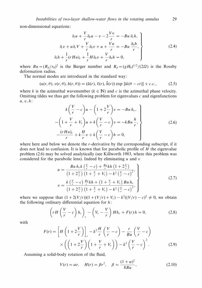
Figure 1. Pressure and velocity fields for Kelvin modes propagating along the outer (a) andthe inner (b) wall with wavenumber k = 2. These modes correspond to (b) and (d ), respectively,in figure 3.

The first pair of roots (2.20) are non-dispersive and correspond to the eigenfunctionu ≡ 0. They, thus, describe the two Kelvin modes concentrated at the inner and outerwalls respectively. We present the elevation profile

h(r) = C1r3 or h(r) = C2r

−3, (2.22)

and the corresponding velocity field obtained from (2.7) and (2.10) for Kelvin modes,with k = 2, in figure 1. The structure of the Kelvin waves with the wind parallel to theboundaries and pressure extrema near the lateral boundaries is clearly seen, as well asthe geostrophic character of the waves. The second pair of roots (2.21) correspond tothe degenerate case (1+2(V/r))(1+ (V/r) +Vr ) − k2((V/r) − c)2 = 0 (see the previoussection). As is easy to see from (2.6), or directly from (2.14) they do not correspondto any non-trivial eigenfunction and will be discarded in what follows.

2.2. Rossby and Poincare modes

The second solution (2.18) combined with (2.12) gives a third-order equation for thephase speed c for each value of n ∈ �:

k2

βBu(α − c)3 −

[k2 + 1 +

(nπ

log( r1r2

)

)+

1 + 2α

βBu

](α − c) + 2(1 + 2α) = 0. (2.23)

For each n ∈ � a set of solutions consists of one Rossby mode and two Poincare(inertia-gravity) modes of order n.

The solutions are given, cf (2.13), by

h(r) = C1r[inπ/log(r1/r2)−1] + C2r

−[inπ/log(r1/r2)−1] (2.24)

with the constraintC1

C2

= − (α − c)α− + (1 + 2α)

(α − c)α− + (1 + 2α)

rα−1

rα+

1

. (2.25)

It should be noted that the case n= 0 ⇒ A= 1 is degenerate: the corresponding fieldmay be obtained, as usual, by taking the limit and leads to the logarithmic in r

solution.The structure of the corresponding modes for k =2 is represented in figure 2: the

Rossby wave in figure 2(a) and the gravity wave in figure 2(b). The characteristic


(a) (b)

Figure 2. Pressure and velocity fields for n= 1 mode of the Rossby wave (a) and the Poincarewave (b) for wavenumber k = 2. These modes correspond to (c) and (a), respectively, in figure 3.

c

k

–1

0

0

1

2

2

3

4 6 8 10

(a)

(b)

(c)

(d)

Figure 3. Dispersion diagram c = c(k) for the solutions of (2.23) and (2.19) with α = 1/2. (a)Poincare modes (see figure 2b), (b) and (d ) Kelvin modes (see figure 1), (c) Rossby modes(see a zoom of this part in figure 4). Note the spectral gap, i.e. the fact that fast Poincare andKelvin modes are separated from slow Rossby modes. Although the spectrum of k is discrete,for the sake of visualization we present continuous curves c(k); it is to be kept in mind thatonly the values k ∈ � correspond to realizable solutions.

velocities and pressure fields of the Rossby wave are easily recognizable with windturning around pressure extrema according to the geostrophic balance.

In figure 3 we present the dispersion diagram for thus obtained eigensolutions ofthe problem (2.6). It is instructive to compare this diagram with the correspondingdiagrams for one-layer shallow-water flow with linear shear (Couette flow) in therectilinear channel in the absence of rotation, as obtained in Knessl & Keller (1995)and Balmforth (1999). In the latter case, Rossby and Kelvin modes are absent; there isno spectral gap and the dispersion curves for left-moving and right-moving Poincaremodes can intersect leading to instability, according to the standard rules (Cairns1979; Sakai 1989). In our case such intersections are not possible due to the spectralgap introduced by rotation, and the flow is stable.

We used the above-described analytic results in order to benchmark the numericalmethod which we are using. The eigenvalue problem of order 3 corresponding to


c

k0 2 4 6 8 10

0.35

0.40

0.45

0.50

0.55

n = 3n = 2

n = 1

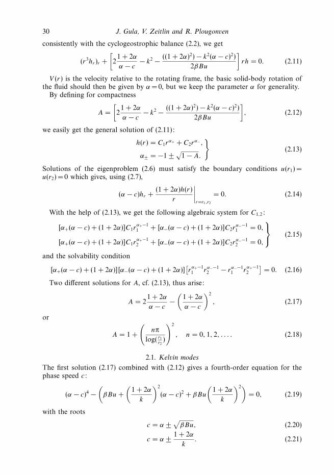
(c)

Figure 4. Zoom of the figure 3 on slow Rossby modes with varying n.

Ω

ΔΩ

ρ1

ρ2H0

r1 r20

Figure 5. Schematic representation of a two-layer flow in the annuluswith a super-rotating lid.

the system of equations (2.6) can be solved numerically by applying the spectralcollocation method as described in Trefethen (2000) and Poulin & Flierl (2003). Acomplete basis of Chebyshev polynomials is used to obtain a discrete equivalent of thesystem which is achieved by evaluating (2.6) on a discrete set of N collocation points(typically a rather low resolution N = 50 to 100 is sufficient, see below) and using theChebyshev differentiation matrix to discretize the spatial derivatives. The eigenvaluesand eigenvectors of the resulting operator are computed with the help of Matlabroutine ‘eig’. The occurrence of spurious eigenvalues is common in such discretizationprocedure. We therefore checked the persistence of the obtained eigenvalues byrecomputing the spectrum with increasing N . The comparison of numerical andanalytic results shows excellent agreement. We do not display it because of absenceof any differences. This means that the collocation method works remarkably welleven at rather low resolution.

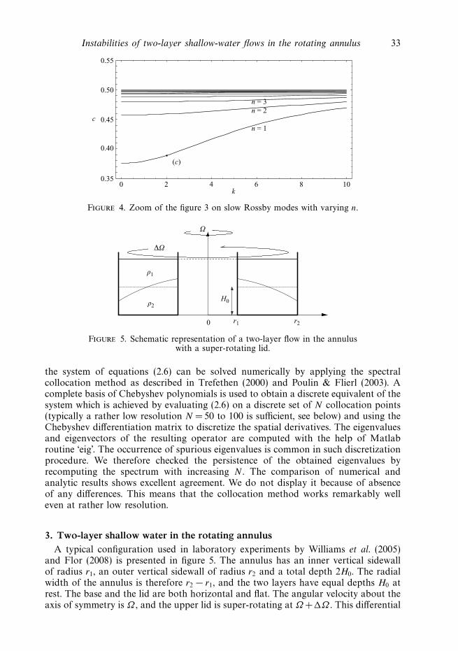
3. Two-layer shallow water in the rotating annulusA typical configuration used in laboratory experiments by Williams et al. (2005)

and Flor (2008) is presented in figure 5. The annulus has an inner vertical sidewallof radius r1, an outer vertical sidewall of radius r2 and a total depth 2H0. The radialwidth of the annulus is therefore r2 − r1, and the two layers have equal depths H0 atrest. The base and the lid are both horizontal and flat. The angular velocity about theaxis of symmetry is Ω , and the upper lid is super-rotating at Ω+�Ω . This differential


rotation provides a vertical velocity shear of the balanced basic state which is close tosolid body rotation of each fluid layer, with different angular velocities. In the stabilityanalysis which follows such state will be represented by a state of cyclogeostrophicequilibrium in each layer with linear radial profile of the azimuthal velocity in therotating two-layer shallow-water model in the f -plane approximation.

In order to fulfil a complete linear stability analysis we use below the collocationmethod, benchmarked in the one-layer case. We present the model, its linearizedversion and introduce the key parameters in § 3.1. We then display the instabilities,their growth rates and the structure of the unstable modes in § 3.2.

3.1. Overview of the model and the method

Consider the two-layer rotating shallow-water model on the f -plane. The momentumand continuity equations are written in polar coordinates as follows:

Djuj −(f +

vj

r

)vj − rΩ2 = ∂rΠj ,

Djvj +(f +

vj

r

)ui =

∂θΠi

r,

Djhj + hj ∇ · vj = 0,

⎫⎪⎪⎪⎬⎪⎪⎪⎭

(3.1)

where vj = (uj , vj ), hj and Πj are the (radial, azimuthal) velocity, thickness andpressure normalized by density (geopotential), in the j th layer (counted from the top)and j = 1, 2. Here, f = 2Ω is the dimensional background rotation and Dj denoteLagrangian derivatives in respective layers. The boundary conditions are u =0 atr = r1, r2.

By introducing the time scale 1/f , the horizontal scale r0 = r2 − r1, the verticalscale H0 and the velocity scale V0 = r0Ω , we use non-dimensional variables fromnow on without changing notation. By linearizing about a steady state with constantazimuthal velocities V1 �= V2, we obtain the following non-dimensional equations (theageostrophic version of the Phillips model in cylindrical geometry):

∂tuj +Vj

r∂θuj − vj − 2

Vjvj

r= −Bu∂rπj ,

∂tvj + uj∂rVj +Vj

r∂θvj + uj +

Vjuj

r= −Bu

∂θπj

r,

∂thj +1

r(rHjuj )r +

1

rHj∂θvj +

Vj

r∂θhj = 0,

⎫⎪⎪⎪⎪⎪⎬⎪⎪⎪⎪⎪⎭

(3.2)

where the pressure perturbations in the layers πj are related through the interfaceperturbation η, as usual:

π2 − π1 + s(π2 + π1) = Bu η, (3.3)

and Bu = (Rd/r0)2 is the Burger number, Ro = �Ω/(2Ω) is the Rossby number,

Rd = (g′H0)1/2/(2Ω) is the Rossby deformation radius, g′ = 2�ρg/(ρ1 + ρ2) is the

reduced gravity and s = (ρ2 − ρ1)/(ρ2 + ρ1) is the stratification parameter.Although the dissipative effects are totally neglected in our analysis we will also

use the following non-dimensional parameter:

d =

√νΩ

H�Ω(3.4)

for the sake of comparison with the experimental results, where for kinematic viscositywe choose the value ν = 1.18.10−6 m2 s−1 which corresponds to the experiments of


Williams et al. (2005). We will also use a parameter F = 1/Bu used as the Froudenumber in Williams et al. (2005) for the same reason.

The depth profiles Hj (r) and respective velocities Vj (r) in (3.2) correspond to steadycyclogeostrophically balanced state in each layer:

2 Vj +V 2

j

r+ r = ∂rΠj . (3.5)

In spite of the introduction of the parameter d , which serves uniquely for scalingpurposes, our analysis is purely inviscid. In the experiment, however, the meanaxisymmetric flow is controlled by friction. Indeed, there is a positive torque due tothe shear across the upper Ekman layer, and there are negative torques due to theshears across the lower Ekman layer and the Stewartson layers at the outer and innervertical sidewalls (Stewartson 1957) acting on the quasi-inviscid interiors of both theupper and lower layers. Because the Stewartson layers are very thin, it seems plausibleto neglect them and to study solutions where each layer rotates as a solid body. Therotation rates of the layers lie in the interval between the rotation rate of the base (0in the rotating frame) and that of the upper lid (Ro in the rotating frame). Therefore,in general,

V2 = α2 r, V1 = α1 r, (3.6)

and we get the following expressions for the heights in the state of cyclogeostrophicequilibrium for such mean flow:

Hj = Hj (0) + (−1)j[2α2 + α2

2 − 2α1 − α21 + s(2α2 + α2

2 + 2α1 + α21 + 2)

] r2

2Bu. (3.7)

Hart (1972) considered the top, bottom and interfacial friction layers and foundthat the rotations rates are α1 = (2 + χ)Ro/2(1 + χ) and α2 = Ro/2(1 + χ) whereχ =(ν2/ν1)

1/2 is the viscosity ratio between the two layers. If the two layers have closeviscosities χ = 1, it leads to (α1, α2) = (0.75 Ro, 0.25 Ro).

A calculation based on a layerwise balance of the torques in Williams, Read &Haine (2004) gives values for (α1, α2) about the same order but depending on theturntable angular velocity. The direct measurements of the radial velocity profiles byFlor (2008) are closer to (α1, α2) ≈ (0.9 Ro, 0.1 Ro). We will therefore keep these lastvalues throughout the paper, but this particular choice does not mean a generalityloss, as changing the relative rotation rate just means rescaling of the Rossby number.

Supposing a harmonic form of the solution in the azimuthal direction,

(uj (r, θ), vj (r, θ), πj (r, θ)) = (uj (r), vj (r), πj (r)) exp[ik(θ − ct)] + c.c., (3.8)

where k is the azimuthal wavenumber (k ∈ �), and omitting tildes we get from (3.2):

k(Vj − rc)iuj − (r + 2Vj )vj + r∂rπj = 0,

−(r + Vj + r∂r (Vj )iuj + k(Vj − rc)vj + kπj = 0,

−∂r (rHj iu) + kHjv + k(Vj − rc)(−1)j η = 0,

π2 − π1 + s(π2 + π1) = Bu η.

⎫⎪⎪⎪⎬⎪⎪⎪⎭

(3.9)

The system (3.9) is an eigenvalue problem of order 6 which can be solved byapplying the spectral collocation method similarly to the one-layer flow. In comparisonto the latter case, the dispersion diagrams we obtain show that the branches ofdispersion relation corresponding to different modes can intersect, thus creatinginstabilities of various nature. Namely, we will display below the instabilities resulting


(a)

(b)

(c)

(d)

10–2 10–1 100 101 102 10310–2

10–1

100

101

0.2

0.3

0.4

0.5

0.6

0.7

0.8

0.9

1.0

Ro

Bu

Outcropping

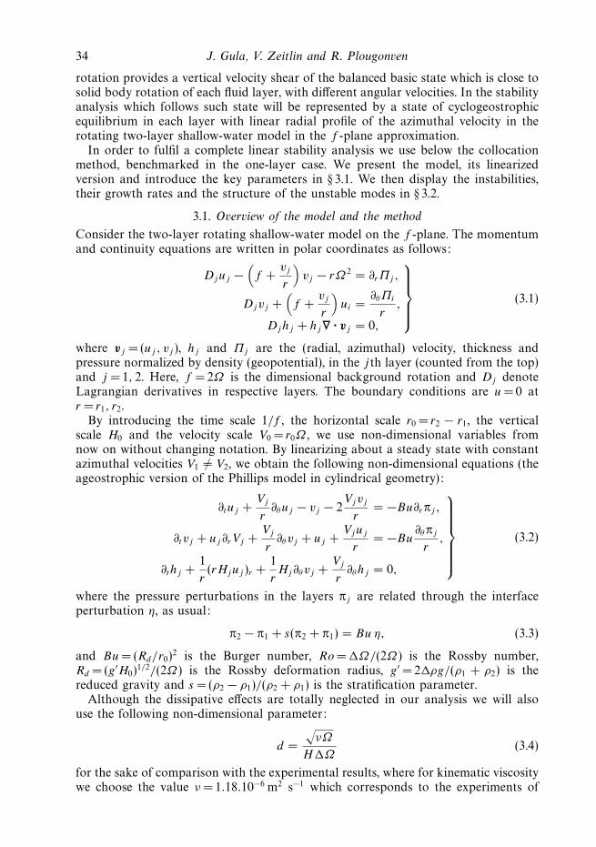
Figure 6. Growth rate of most unstable modes in (Ro,Bu) space. Darker zones correspondto higher growth rates. Contours displayed are 0.001, 0.01, 0.02 and further interval at 0.02.The thick upper frontier line marks the outcropping limit when the interface between the twolayers intersects the bottom or the top. The results for the outcropping configuration will benot discussed in this paper.

from the interaction between Rossby waves in upper and lower layer (the baroclinicinstability), the interaction between Rossby and Kelvin or Poincare waves in respectivelayers (RK instability) and the interaction between two Poincare, or Kelvin andPoincare, or two Kelvin modes (KH instability). Although each instability occupiesits proper domain in the parameter space, we will see that there exist crossover regionswhere two different instabilities coexist and may compete.

3.2. Instabilities and growth rates

We first present the overall stability diagram in the space of parameters of the model,and then illustrate different parts of this diagram by displaying the correspondingunstable modes and dispersion curves. The stability diagram was obtained bycalculating the eigenmodes and the eigenvalues of the problem (3.6), (3.9) for about50 000 points in the space of parameters (there are typically 200–300 points along eachaxis in the figures below) and then interpolating. As before, only discrete azimuthalwavenumbers correspond to realizable modes. We nevertheless present the results asif the spectrum of wavenumbers were continuous, for better visualization.

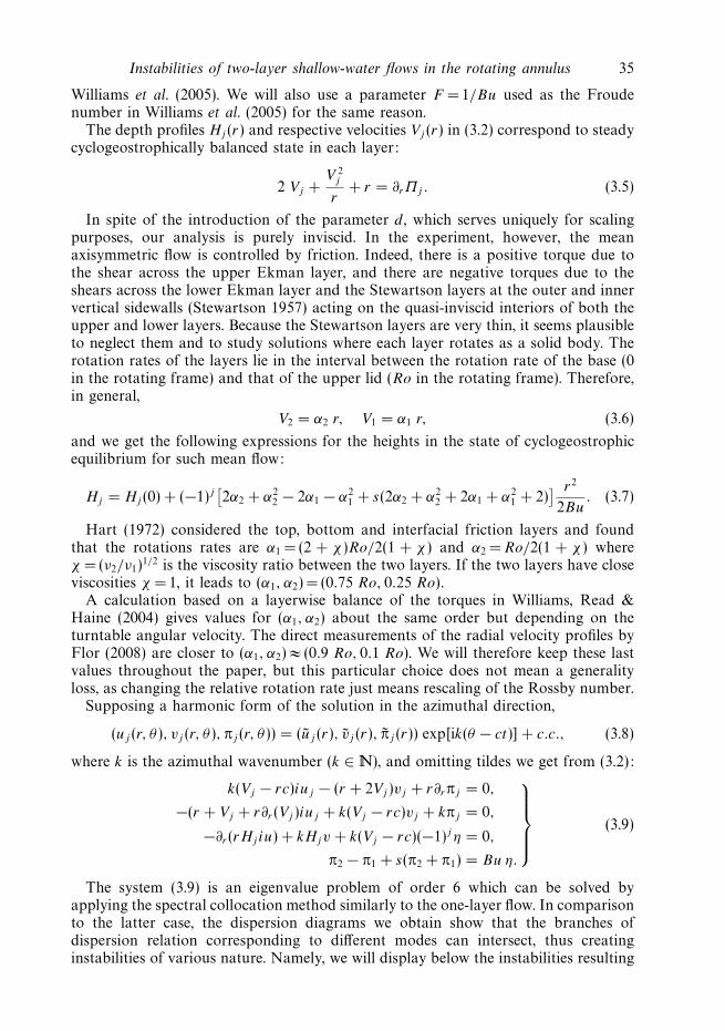
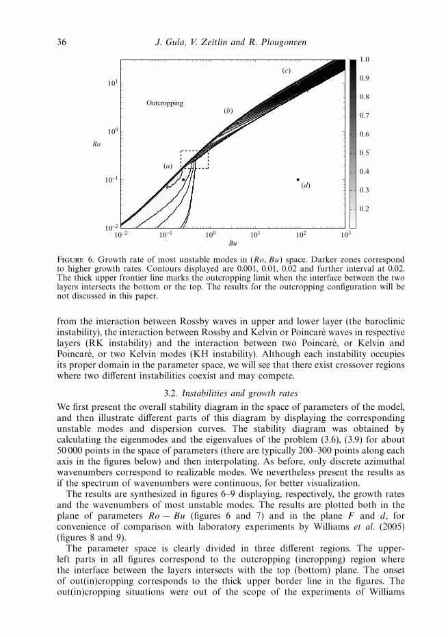
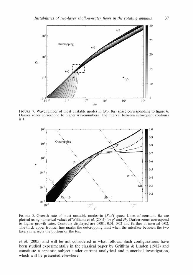
The results are synthesized in figures 6–9 displaying, respectively, the growth ratesand the wavenumbers of most unstable modes. The results are plotted both in theplane of parameters Ro − Bu (figures 6 and 7) and in the plane F and d , forconvenience of comparison with laboratory experiments by Williams et al. (2005)(figures 8 and 9).

The parameter space is clearly divided in three different regions. The upper-left parts in all figures correspond to the outcropping (incropping) region wherethe interface between the layers intersects with the top (bottom) plane. The onsetof out(in)cropping corresponds to the thick upper border line in the figures. Theout(in)cropping situations were out of the scope of the experiments of Williams


(a)

(b)

(c)

(d)

10

5

15

20

25

30

Outcropping

10–2

10–1

100

101

Ro

10–2 10–1 100 101 102 103

Bu

Figure 7. Wavenumber of most unstable modes in (Ro,Bu) space corresponding to figure 6.Darker zones correspond to higher wavenumbers. The interval between subsequent contoursis 1.

102

101

100

F

10–1

10–2

Outcropping (a)

(b)

(d)

(c)

Ro = 10 Ro = 1

Ro = 0.1

10–3

10–3 10–2

1.0

0.9

0.8

0.7

0.6

0.5

0.4

0.3

0.2

10–1

d

Figure 8. Growth rate of most unstable modes in (F, d) space. Lines of constant Ro areplotted using numerical values of Williams et al. (2005) for g′ and H0. Darker zones correspondto higher growth rates. Contours displayed are 0.001, 0.01, 0.02 and further at interval 0.02.The thick upper frontier line marks the outcropping limit when the interface between the twolayers intersects the bottom or the top.

et al. (2005) and will be not considered in what follows. Such configurations havebeen studied experimentally in the classical paper by Griffiths & Linden (1982) andconstitute a separate subject under current analytical and numerical investigation,which will be presented elsewhere.


102

101

100

F

10–1

10–2

10–3

10–3 10–2 10–1

d

30

25

20

15

10

5

Outcropping

(b)

Ro = 10

(a)

(c)

(d)

Ro = 1

Ro = 0.1

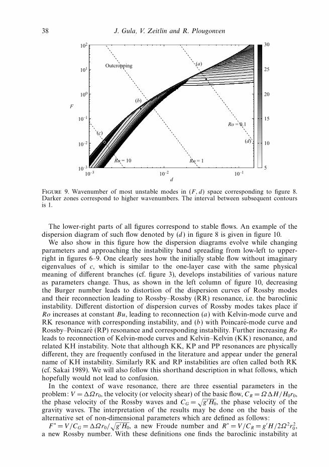
Figure 9. Wavenumber of most unstable modes in (F, d) space corresponding to figure 8.Darker zones correspond to higher wavenumbers. The interval between subsequent contoursis 1.

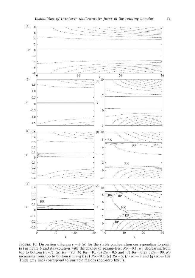
The lower-right parts of all figures correspond to stable flows. An example of thedispersion diagram of such flow denoted by (d ) in figure 8 is given in figure 10.

We also show in this figure how the dispersion diagrams evolve while changingparameters and approaching the instability band spreading from low-left to upper-right in figures 6–9. One clearly sees how the initially stable flow without imaginaryeigenvalues of c, which is similar to the one-layer case with the same physicalmeaning of different branches (cf. figure 3), develops instabilities of various natureas parameters change. Thus, as shown in the left column of figure 10, decreasingthe Burger number leads to distortion of the dispersion curves of Rossby modesand their reconnection leading to Rossby–Rossby (RR) resonance, i.e. the baroclinicinstability. Different distortion of dispersion curves of Rossby modes takes place ifRo increases at constant Bu, leading to reconnection (a) with Kelvin-mode curve andRK resonance with corresponding instability, and (b) with Poincare-mode curve andRossby–Poincare (RP) resonance and corresponding instability. Further increasing Ro

leads to reconnection of Kelvin-mode curves and Kelvin–Kelvin (KK) resonance, andrelated KH instability. Note that although KK, KP and PP resonances are physicallydifferent, they are frequently confused in the literature and appear under the generalname of KH instability. Similarly RK and RP instabilities are often called both RK(cf. Sakai 1989). We will also follow this shorthand description in what follows, whichhopefully would not lead to confusion.

In the context of wave resonance, there are three essential parameters in theproblem: V = �Ωr0, the velocity (or velocity shear) of the basic flow, CR = Ω�H/H0r0,the phase velocity of the Rossby waves and CG =

√g′H0, the phase velocity of the

gravity waves. The interpretation of the results may be done on the basis of thealternative set of non-dimensional parameters which are defined as follows:

F ∗ = V/CG = �Ωr0/√

g′H0, a new Froude number and R∗ = V/CR = g′H/2Ω2r20 ,

a new Rossby number. With these definitions one finds the baroclinic instability at


8

6

4

2

0

–2

–4

–6

–8100 20

10

5

0

10

8

6

4

2

0

10

8

6

4

2

0

–2

–2

c

c

c

–5

k 30

100

RR

RK

RK

RK RP

KK

KP

RP

RP RP

20

k

30 100 20

k

30

1.5

1.0

0.5

0

–0.5

–1.0

–1.5

0.5

0.4

0.3

0.2

0.1

0

–0.1

–0.2

–0.3

–0.4

0.4

0.3

0.2

0.1

0

–0.1

–0.2

–0.3

c

c

c

c

(a)

(b)

(c)

(d)

(e)

(f)

(g)

Figure 10. Dispersion diagram c − k (a) for the stable configuration corresponding to point(d ) in figure 6 and its evolution with the change of parameters: Ro = 0.1, Bu decreasing fromtop to bottom ((a–d ): (a) Bu =90, (b) Bu =10, (c) Bu =0.5 and (d ) Bu =0.25); Bu =90, Roincreasing from top to bottom ((a, e–g): (a) Ro = 0.1, (e) Ro = 5, (f ) Ro = 8 and (g) Ro =10).Thick grey lines correspond to unstable regions (non-zero Im(c)).


σ

c

k

RR

2 4 6 8 10 12 14 16 18 20

0.01

0.02

0.03

0.04

0.05

0.1

(a)

(b)

0

0

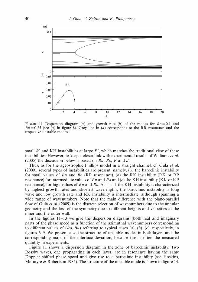
Figure 11. Dispersion diagram (a) and growth rate (b) of the modes for Ro = 0.1 andBu =0.25 (see (a) in figure 8). Grey line in (a) corresponds to the RR resonance and therespective unstable modes.

small R∗ and KH instabilities at large F ∗, which matches the traditional view of theseinstabilities. However, to keep a closer link with experimental results of Williams et al.(2005) the discussion below is based on Bu, Ro, F and d .

Thus, as for the ageostrophic Phillips model in a straight channel, cf. Gula et al.(2009), several types of instabilities are present, namely, (a) the baroclinic instabilityfor small values of Bu and Ro (RR resonance), (b) the RK instability (RK or RPresonance) for intermediate values of Bu and Ro and (c) the KH instability (KK or KPresonance), for high values of Bu and Ro. As usual, the KH instability is characterizedby highest growth rates and shortest wavelengths, the baroclinic instability is longwave and low growth rate and RK instability is intermediate, although spanning awide range of wavenumbers. Note that the main difference with the plane-parallelflow of Gula et al. (2009) is the discrete selection of wavenumbers due to the annulargeometry and the loss of the symmetry due to different heights and velocities at theinner and the outer wall.

In the figures 11–13 we give the dispersion diagrams (both real and imaginaryparts of the phase speed as a function of the azimuthal wavenumber) correspondingto different values of (Ro, Bu) referring to typical cases (a), (b), (c), respectively, infigures 6–9. We present also the structure of unstable modes in both layers and thecorresponding maps of the interface deviation, because this is often the measuredquantity in experiments.

Figure 11 shows a dispersion diagram in the zone of baroclinic instability. TwoRossby waves, one propagating in each layer, are in resonance having the sameDoppler shifted phase speed and give rise to a baroclinic instability (see Hoskins,McIntyre & Robertson 1985). The structure of the unstable mode is shown in figure 14.


RK

RP

RK

1.0

2.0(a)

(b)

0.2

0.4

0.6

0.8

0.5

1.5

0

0

σ

c

k2 4 6 8 10 12 14 16 18 20

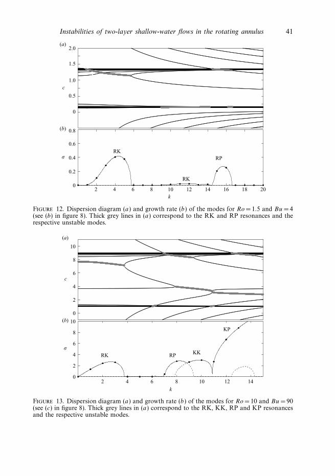
Figure 12. Dispersion diagram (a) and growth rate (b) of the modes for Ro = 1.5 and Bu = 4(see (b) in figure 8). Thick grey lines in (a) correspond to the RK and RP resonances and therespective unstable modes.

k

RK RPKK

KP

2

2

2

4

4

4

6

6

6

8

8

8

10

10

10

(a)

(b)

12 140

0

σ

c

Figure 13. Dispersion diagram (a) and growth rate (b) of the modes for Ro = 10 and Bu =90(see (c) in figure 8). Thick grey lines in (a) correspond to the RK, KK, RP and KP resonancesand the respective unstable modes.


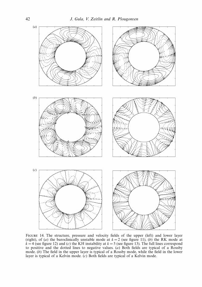
(a)

(b)

(c)

Figure 14. The structure, pressure and velocity fields of the upper (left) and lower layer(right), of (a) the baroclinically unstable mode at k =2 (see figure 11), (b) the RK mode atk = 4 (see figure 12) and (c) the KH instability at k = 5 (see figure 13). The full lines correspondto positive and the dotted lines to negative values. (a) Both fields are typical of a Rossbymode. (b) The field in the upper layer is typical of a Rossby mode, while the field in the lowerlayer is typical of a Kelvin mode. (c) Both fields are typical of a Kelvin mode.


(a)

(b)

(c)

Figure 15. Interface height for (a) baroclinic instability at k = 2 (see figure 11), (b) RKinstability at k = 4 (see figure 12) and (c) KH instability at k = 5 (see figure 13). The full linescorrespond to positive and the dotted lines to negative values. Contours are plotted at theinterval (a) 0.0137, (b) 0.015 and (c) 0.017.

Figure 12 shows a dispersion diagram in a pure RK instability area. A Rossbywave propagating in the upper layer resonates with a Kelvin wave propagating in thelower layer and give rise to a RK instability (see Sakai 1989; Gula et al. 2009). Thestructure of the unstable mode is shown in figure 14.


0.1

0.2

0.3

0.4

0.5

0.6

0.7

0.8

0.9

Ro

Bu

(e)

Figure 16. Growth rate of most unstable modes in (Ro,Bu) space. Zoom of the box infigure 6. Contours displayed are 0.001, 0.01, 0.02 and further interval at 0.02.

Figure 13 shows a dispersion diagram in a KH instability area. A Kelvin wavepropagating in the upper layer resonates with another Kelvin wave propagating inthe lower layer and gives rise to a KH instability. For these values of parameters wecan see that RP and RK instabilities are also present but with lower growth rates.The structure of the unstable mode is shown in figure 14.

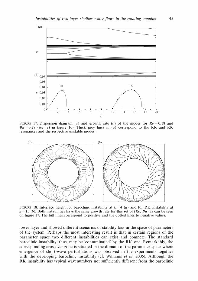
Thus RK and KH instabilities coexist for large Bu and Ro (small F and d) havingcomparable growth rates, although different characteristic wavenumbers. As followsfrom the last figure, and from the comparison of figures 8 and 9, or 6 and 7, in general,close values of the growth rates may correspond to essentially different wavelengthsof the most unstable modes. This means that different instabilities may coexist andcompete. A clear-cut crossover region is indicated by a box in figures 8 and 9, andcorresponds to coexisting baroclinic and RK instabilities. A zoom of the box is shownin figure 16.

Figure 17 shows the dispersion diagram corresponding to the (e) point in thecrossover region of figure 16. We see that in this area both baroclinic and RKinstability are present, having close growth rates. This means that the two instabilitiesare competing and that relatively high wavenumbers may be excited due to the RKinstability in this range of parameters. The interface deviations corresponding tocompeting RR and RK instabilities are presented in figure 18.

4. Summary and discussionThus, after having analytically resolved the problem of small perturbations around

cyclogeostrophycally balanced one-layer shallow-water Couette flow in the rotatingannulus, which allowed us (a) to identify the normal modes of the problem and (b) tobenchmark the numerical collocation scheme, we established a full stability diagramof the two-layer vertically sheared flow in the rotating annulus and identified themain instability modes. We established the origin of various instabilities resultingfrom phase-locking and resonance between the normal modes of the upper and the


RKRR

0.01

0.02

0.03

0.04

0.05

0.06

0

0

(a)

(b)

σ

c

k2 4 6 8 10 12 14 16 18 20

Figure 17. Dispersion diagram (a) and growth rate (b) of the modes for Ro = 0.18 andBu = 0.28 (see (e) in figure 16). Thick grey lines in (a) correspond to the RR and RKresonances and the respective unstable modes.

(a) (b)

Figure 18. Interface height for baroclinic instability at k = 4 (a) and for RK instability atk =15 (b). Both instabilities have the same growth rate for this set of (Ro, Bu) as can be seenon figure 17. The full lines correspond to positive and the dotted lines to negative values.

lower layer and showed different scenarios of stability loss in the space of parametersof the system. Perhaps the most interesting result is that in certain regions of theparameter space two different instabilities can exist and compete. The standardbaroclinic instability, thus, may be ‘contaminated’ by the RK one. Remarkably, thecorresponding crossover zone is situated in the domain of the parameter space whereemergence of short-wave perturbations was observed in the experiments togetherwith the developing baroclinic instability (cf. Williams et al. 2005). Although theRK instability has typical wavenumbers not sufficiently different from the baroclinic


one (cf. figure 17) and, thus, cannot directly explain the experimental observations ofsmall-scale waves on top of the developing baroclinic instability, the interaction of twodifferent unstable modes is worth studying in this context. Note that as shown in Gulaet al. (2009), the nonlinear saturation of the RK instability is totally different fromthat of baroclinic instability, with an important role being played by the mean flowreorganisation. Thus, although on general grounds one could expect manifestationsof the standard behaviour of the pair of nonlinear modes, like e.g. synchronization,it is difficult to make predictions without detailed studies of the nonlinear regime.The finite amplitude disturbances and the effects of nonlinearity as the nonlinearinteractions between the various waves will be investigated in future work, boththeoretically and by using a high-resolution finite-volume numerical scheme and amesoscale atmospheric model (WRF).

Coming back to the main motivation of our study, the comparison between ourresults and laboratory experiments shows good agreement in some parameter regions,and discrepancies in some other. Let us look at the figure 8 and at the correspondingfigure in Williams et al. (2005). While there is a very good agreement in the baroclinicinstability region, the region of the KH instability in figure 8 is relatively narrowcompared to Williams et al. (2005). As to the RK instability region, it is not clearlyidentifiable in the experiment.

An obvious explanation of the first discrepancy is that, in spite of the same physicalmechanism, the KH instabilities in shallow-water and in full primitive equations arenot quantitatively the same, especially in the large wavenumber domain. Anotherfactor is surface tension. According to Hart (1972) and James (1977), the interfacialsurface tension between the two layers is negligible for the long-wave instabilities,while it is stabilizing for short- wave ones. Indeed, the effect of interfacial surfacetension is inversely proportional to the wavelength square. The short-wave RKand KH instabilities are then likely to be stabilized, while the long-wave baroclinicinstability is unaffected.

Another possible explanation of non-manifestation of the RK instability is its rapidnonlinear saturation due to reorganisation of the mean flow and energy dissipationthrough small scale secondary KH instabilities (cf. Gula et al. 2009), which makes itmore difficult to identify in a laboratory experiment such as Williams et al. (2005),especially in view of the small dimensions of the apparatus.

As was already stressed in the Introduction, the two-layer rotating shallow-watermodel should be considered as a conceptual one, allowing to grasp the universalfeatures of destabilization of large-scale shear flows in GFD. In principle, a linearstability analysis of a full (three-dimensional, non-hydrostatic, viscous and surfacetension included) experimental flow is possible along the same lines. However, suchtask requires incommensurate (with respect to its ‘coarse-grained’ shallow-watercounterpart) computational efforts, and the results will depend on the fine structureof the mean flow (e.g. the parameters of the mixing layer between the layers) whichmay vary from one experiment to another.

The authors are grateful to anonymous reviewers for useful comments. This workwas supported by ANR project FLOWINg (BLAN06-3 137005) and Alliance project15102ZJ.

REFERENCES

Balmforth, N. J. 1999 Shear instability in shallow water. J. Fluid Mech. 387, 97–127.

Cairns, R. A. 1979 The role of negative energy waves in some instabilities of parallel flows. J. FluidMech. 92, 1–14.


Dunkerton, T., Lelong, P. & Snyder, C. (Ed.) 2008 Spontaneous imbalance. J. Atmos. Sci. webpage:http://ams.allenpress.com/perlserv/?request=get-collection&coll id=20&ct=1.

Flor, J. B. 2008 Frontal instability, inertia-gravity wave radiation and vortex formation. InProceedings of the ICMI International Conference on Multimodal Interfacings, London, UK.

Ford, R. 1994 Gravity wave radiation from vortex trains in rotating shallow water. J. Fluid Mech.281, 81–118.

Fultz, D., Long, R. R., Owens, G. V., Bohan, W., Kaylor, R. & Weil, I. 1959 Studies of thermalconvection in a rotating cylinder with some implications for large-scale atmospheric motions.Meteorol. Monogr. 4, 1–104.

Griffiths, R. W. & Linden, P. F. 1982 Part I. Density-driven boundary currents. Geophys. Astrophys.Fluid Dyn. 19, 159–187.

Gula, J., Plougonven, R. & Zeitlin, V. 2009 Ageostrophic instabilities of fronts in a channel inthe stratified rotating fluid. J. Fluid Mech. 627, 485–507.

Hart, J. E. 1972 A laboratory study of baroclinic instability. Geophys. Astrophys. Fluid Dyn. 3,181–209.

Hide, R. 1958 An experimental study of thermal convection in a rotating liquid. Phil. Trans. R. Soc.Lond. Ser. A, Math. Phys. Sci. 250 (983), 441–478.

Hide, R. & Fowlis, W. W. 1965 Thermal convection in a rotating annulus of liquid: effect of viscosityon the transition between axisymmetric and non-axisymmetric flow regimes. J. Atmos. Sci. 22,541–558.

Hoskins, B. J., McIntyre, M. E. & Robertson, A. W. 1985 On the use and significance of isentropicpotential vorticity maps. Quart. J. R. Meteorol. Soc. 111 (470), 877–946.

James, I. N. 1977 Stability of flow in a slowly rotating two-layer system. Occasional Note Met Office27/77/2 unpublished.

Killworth, P. D. 1983 On the motion of isolated lenses on a beta-plane. J. Phys. Oceanogr. 13,368–376.

Knessl, C. & Keller, J. B. 1995 Stability of linear shear flows in shallow water. J. Fluid Mech. 303,203–214.

Lovegrove, A. F., Read, P. L. & Richards, C. J. 2000 Generation of inertia-gravity waves in abaroclinically unstable fluid. Quart. J. R. Meteorol. Soc. 126, 3233–3254.

O’Sullivan, D. & Dunkerton, T. J. 1995 Generation of inertia-gravity waves in a simulated lifecycle of baroclinic instability. J. Atmos. Sci. 52 (21), 3695–3716.

Poulin, F. J. & Flierl, G. R. 2003 The nonlinear evolution of barotropically unstable jets. J. Phys.Oceanogr. 33, 2173–2192.

Sakai, S. 1989 Rossby–Kelvin instability: a new type of ageostrophic instability caused by aresonance between Rossby waves and gravity waves. J. Fluid Mech. 202, 149–176.

Stewartson, K. 1957 On almost rigid rotations. J. Fluid Mech. 3, 17–26.

Trefethen, L. N. 2000 Spectral Methods in Matlab. Society for Industrial and Applied Mathematics.

Williams, P. D., Haine, T. W. N. & Read, P. L. 2005 On the generation mechanisms of short-scaleunbalanced modes in rotating two-layer flows with vertical shear. J. Fluid Mech. 528, 1–22.

Williams, P. D., Read, P. L. & Haine, T. W. N. 2004 A calibrated, non-invasive method formeasuring the internal interface height field at high resolution in the rotating, two-layerannulus. Geophys. Astrophys. Fluid Dyn. 98, 453–471.

Documents

Instabilities of two-layer shallow-water ﬂows with