Innovative Growth AccountingINNOVATIVE GROWTH ACCOUNTING 3 We exploit ﬁrm and plant data on employment at all nonfarm businesses from 1983–2013 in the U.S. Census Bureau’s Longitudinal

Innovative Growth Accounting

Peter J. Klenow

Stanford University

Huiyu Li∗

Federal Reserve Bank of SF

March 23, 2020

Abstract

Recent work highlights a falling entry rate of new firms and a risingmarket share of large firms in the United States. To understand how thesechanging firm demographics have affected growth, we decompose produc-tivity growth into the firms doing the innovating. We trace how much eachfirm innovates by the rate at which it opens and closes plants, the marketshare of those plants, and how fast its surviving plants grow. Using data onall nonfarm businesses from 1982–2013, we find that new and young firms(ages 0 to 5 years) account for almost one-half of growth — three times theirshare of employment. Large established firms contribute only one-tenthof growth despite representing one-fourth of employment. Older firms doexplain most of the speedup and slowdown during the middle of our sam-ple. Finally, most growth takes the form of incumbents improving their ownproducts, as opposed to creative destruction or new varieties.

∗Klenow: Stanford University and NBER; Li: Federal Reserve Bank of San Francisco. Wethank Mark Bils, Chang-Tai Hsieh, and Erik Hurst for useful comments. We also thank AmberFlaharty and Gladys Teng for excellent research assistance. Any opinions and conclusions ex-pressed herein are those of the author(s) and do not necessarily represent the views of the U.S.Census Bureau or the Federal Reserve System. This research was performed at a Federal Statis-tical Research Data Center under FSRDC Project Number 1440. All results have been reviewedto ensure that no confidential information is disclosed.

2 KLENOW AND LI

1. Introduction

Solow (1956) famously decomposed output growth into contributions from cap-

ital, labor, and productivity. Mankiw, Romer and Weil (1992) further decom-

posed productivity into human capital versus residual productivity. We take this

residual productivity, routinely calculated by the U.S. Bureau of Labor Statistics,

as our starting point. We attribute productivity growth to innovation and ask:

what form does the innovation take, and which firms do most of the innovation?

Innovation can take the form of a stream of new varieties that are not close

substitutes for any existing varieties (Romer, 1990). Alternatively, growth could

be driven by creative destruction of existing products as in Aghion and Howitt

(1992). Examples include Walmart stores driving out mom-and-pop stores or

Amazon stealing business from physical stores. Yet another possibility is that

growth takes the form of existing producers improving their own products (e.g.,

successive generations of Apple iPhones or new car models). Even conditional

on the form of innovation, growth could be led by entrants and young firms

(e.g., Uber or Netflix) or by older and larger firms (e.g., Intel or Starbucks).

U.S. productivity growth has been lackluster in recent decades, except for

a decade-long surge from the mid-1990s through the mid-2000s.1 At the same

time, firm entry rates have fallen and reallocation of labor across incumbent

firms has slowed — coined “declining business dynamism” by papers such as

Decker, Haltiwanger, Jarmin and Miranda (2014). Large, established superstar

firms have captured a bigger share of markets. Is this declining dynamism and

rising concentration responsible for the growth slowdown? Have superstar firms

helped growth or hindered it?

We offer a new growth decomposition to shed light on these questions. We

decompose growth into three types of innovation: creative destruction, brand

new varieties, and innovation by incumbents on their own products. We further

decompose each of these sources into contributions by firm age and size.

1See Fernald (2015) for discussion on the timing of the productivity speedup and slowdown.

INNOVATIVE GROWTH ACCOUNTING 3

We exploit firm and plant data on employment at all nonfarm businesses

from 1983–2013 in the U.S. Census Bureau’s Longitudinal Business Database

(LBD). We treat each plant as a unique product (or set of products). This en-

ables us to observe the rate and importance of product entry and exit across

firms. We rely on a model in which employment at a plant is isoelastic with

respect to the quality of products produced at the plant.2 We use the size of

entering versus exiting plants to gauge the quality of brand new products and

the quality improvements made through creative destruction. We assess qual-

ity improvements by firms on their own products using changes in employment

over time at surviving incumbent plants. We also allow the lowest quality prod-

ucts (plants) to exit due to obsolescence (i.e, inability to keep up with overall

quality and variety growth) as in Hopenhayn (1992).3

We preview our findings as follows. Some 60% of growth on average comes

from incumbent innovations on their own products, whereas about 27% comes

from new varieties and 13% from creative destruction. Many exiting plants are

quite small, suggesting much of exit is due to obsolescence rather than creative

destruction. And new plants are smaller than incumbent plants on average,

making us infer that most plant entry takes the form of new varieties rather

than creative destruction.

We find that own innovation drove both the mid-1990s speedup and the

mid-2000s slowdown of growth. TFP growth averaged 1.15% per year from 1982–

1995, then sped up to 2.82% per year from 1996–2005 before falling back to

1.03% per year from 2006–2013. Own innovation accounted for 148 of the 167

basis point acceleration, and 144 of the 179 basis point deceleration. Even

though entry and job reallocation fell throughout the sample, growth from cre-

ative destruction accelerated modestly from 1996–2005 versus 1982–1995.

2We model product heterogeneity as coming from quality differences, but these will be iso-morphic to differences in process efficiency in our model setting.

3We do not model the arrival rates and step sizes of innovation, but rather back them outfrom data moments in the LBD. We allow them to vary over time and across firms. In this sense,we are not assuming these arrival rates and step sizes are exogenous. Instead, we are estimatingand carrying out a model-based growth decomposition.

4 KLENOW AND LI

New firms in a given year account for about 1/3 of growth on average. New

and young firms (ages 0–5 years) together contribute roughly 1/2 of all growth,

despite employing less than 1/5 of all workers. Older incumbents (ages 6 and

above) contribute the other half of growth. Such established firms played a big-

ger role in the speedup and slowdown of growth, however, accounting for 80%

of the pickup and 70% of the dropoff.

The largest firms — those with 5,000 or more workers — accounted for only

11% of growth on average. This is less than half of their 25% share of employ-

ment. Small firms, with fewer than 20 employees, explain over 60% of growth

despite employing only 21% of all workers. This is very much in the spirit of

Haltiwanger, Jarmin and Miranda (2013), who emphasize the outsized contri-

bution of young, small fast-growing firms (“gazelles”) to gross job creation.

The speedup and slowdown of growth occurred uniformly across the size

distribution. In particular, firms with (i) less than 20 employees, (ii) between 20

and 249 employees, (iii) between 250 and 4999 employees, and (iv) 5000 or more

employees, each produced a speedup and slowdown of around 40 basis points.

Thus, in this accounting, superstar firms did not generate the bulk of the boom

or bust. Focusing on the role of superstars in creating or hindering growth —

at least directly — seems misplaced. It is possible, of course, that the rise of

superstar firms discouraged innovation by other firms, as in Aghion, Bergeaud,

Boppart, Klenow and Li (2020).

The rest of the paper proceeds as follows. Section 2 relates our paper to the

existing literature. Section 3 lays out the model we use to do innovation ac-

counting. Section 4 presents the mapping from model parameters to the mo-

ments in the LBD. Section 5 provides our main results. Section 6 discusses fur-

ther results and directions for future research. Section 7 concludes.


2. Related Literature

The classic reference on creative destruction models is Aghion and Howitt (1992).

Klette and Kortum (2004) developed potential implications of creative destruc-

tion for firm dynamics. Lentz and Mortensen (2008) formally estimated a gen-

eralization of the Klette-Kortum model using data on Danish firms. See Aghion,

Akcigit and Howitt (2014) for a survey of the literature on both models and evi-

dence of creative destruction. Aghion, Bergeaud, Boppart, Klenow and Li (2019)

analyze how creative destruction can be missed in measures of aggregate pro-

ductivity growth. Hsieh, Klenow and Nath (2019) develop and calibrate a two-

country version of the Klette-Kortum model.

Romer (1990) is the seminal paper on expanding variety models. Rivera-

Batiz and Romer (1991) followed up with a two-economy version. Acemoglu

(2003) and Jones (2016) are two of many subsequent models built around va-

riety growth. Chapter 12 of Acemoglu (2011) provides a textbook treatment.

Feenstra (1994) and Broda and Weinstein (2006) estimate variety gains from im-

ports. Broda and Weinstein (2006) estimate growth in the range of consumer

products available.

Krusell (1998) was an early paper modeling innovation by incumbent firms

on their own products. Lucas and Moll (2014) can be interpreted to be in this

vein. See chapter 12 of Aghion and Howitt (2009) and chapter 14 of Acemoglu

(2011) for models combining own innovation with creative destruction. Other

papers with multiple types of innovation include Luttmer (2011), Akcigit and

Kerr (2018), and Peters (2019). Atkeson and Burstein (2019) analyze optimal

policy in the presence multiple innovation channels. They emphasize that the

social return to creative destruction is smaller than to own innovation or to the

creation of new varieties. From a policy perspective, therefore, we care about

the importance of each type of innovation in overall growth.

Perhaps the closest paper to ours is Garcia-Macia, Hsieh and Klenow (2019).

They too use LBD data to infer the types of innovation behind U.S. growth in

6 KLENOW AND LI

recent decades. The key distinction is that they look only at firms. By exploit-

ing data on plants and assuming plants proxy for varieties produced by a firm,

we are able to directly infer the sources of growth. Garcia-Macia et al. resort

to indirect inference, and also make simplifying assumptions such as that the

step-size of innovations is the same for own innovation and creative destruc-

tion. We are able to relax this assumption, and even allow step sizes for all types

of innovation to differ by the size and age of firms.

Our model also features exit of the lowest quality products due to obsoles-

cence. Hopenhayn (1992) is a pioneering model with this feature. Hopenhayn,

Neira and Singhania (2018) is a recent application to understand the falling en-

try rate. Akcigit and Ates (2019) and Peters and Walsh (2019) analyze the causes

of both falling entry and falling growth. Other efforts to explain lackluster recent

growth include Engbom (2017) and Liu, Mian and Sufi (2019).

Our approach builds on Feenstra (1994), which infers quality and variety

growth from a product’s market share. Feenstra showed that one can back out

underlying quality and variety using a CES demand elasticity and the market

share of a product. Hottman, Redding and Weinstein (2016) follow the Feen-

stra approach, and have the advantage of directly seeing products at a detailed

level. They also observe prices and quantities, so they can adjust for markups

when inferring a product’s quality. Due to data constraints, we abstract from

markup dispersion across products. The tradeoff is that we look beyond con-

sumer packaged goods to the entire nonfarm business sector.

With data on prices and quantities and products, one could adjust not only

for markups but for other factors driving a wedge between a plant’s employ-

ment and the quality and variety of its products. This includes adjustment

costs, financial frictions, and capital intensity of production. One could fo-

cus more narrowly on U.S. manufacturing and control for such factors. Follow-

ing Foster, Haltiwanger and Syverson (2008), one could separate “TFPQ” from

“TFPR” by netting out the influence of markups, adjustment costs, factor inten-

sity and so on — and then apply our direct inference to TFPQ data to determine


the sources of innovation. See Hsieh and Klenow (2009, 2014) and Eslava and

Haltiwanger (2019) for efforts along these lines.

Just as growth accounting does not require that capital or labor be deter-

mined exogenously, our innovative growth accounting does not require that in-

novation rates be exogenous. For this reason, our accounting is not inconsistent

with the literature arguing that innovation rates are sustained only because of

growth in research efforts. See, for example, Jones (1995) and Bloom, Jones,

Van Reenen and Webb (2017).

Less consistent with our approach are decompositions of productivity growth

into within-firm, reallocation, and entry-exit terms by Baily, Hulten and Camp-

bell (1992), Griliches and Regev (1995), Olley and Pakes (1996), and Melitz and

Polanec (2015). A prominent implementation is Foster, Haltiwanger and Krizan

(2001), and more recent versions are Decker, Haltiwanger, Jarmin and Miranda

(2017) and Gutierrez and Philippon (2019). Baqaee and Farhi (2020) show that

such statistical decompositions are not derived from explicit general equilib-

rium models. Thus, although these decompositions provide useful moments

that models should match, they do not provide a direct way to infer the sources

of innovation and growth.

In particular, the above decompositions use growth in firm labor productiv-

ity to evaluate innovation within firms. Figures 1 and 2 compare growth in rev-

enue per worker (labor productivity) to growth in employment for Walmart and

Amazon based on Compustat data.4 For Walmart, employment grew rapidly

while labor productivity grew comparatively little. For Amazon, revenue pro-

ductivity did grow markedly, but employment growth was much faster still. Fig-

ures 3 through 7 in the Appendix cover Microsoft, Google, Facebook, Apple and

Starbucks. In all of these firms employment growth dwarfed growth in revenue

per worker. All of these firms were famously innovative. The consistent byprod-

4The Census LBD, which we use for almost all of our estimates, does not have data on rev-enue, and the U.S. Census Bureau forbids us from revealing the identity of firms. Hence wecompare measures of revenue labor productivity with employment growth for innovative firmsin Compustat.

8 KLENOW AND LI

Figure 1: Walmart

Figure 2: Amazon

Source: WRDS Compustat and BEA Table 1.1.9. Revenue per worker = “REVT / (GDP Deflator x

EMP)”, Employment = “EMP” and Year = “FYEAR”. The graph displays revenue per worker and

employment relative to the first year when both series are available for the firm.


uct of their innovation would appear to be swift employment growth rather than

revenue productivity growth. This suggests their innovation may have taken

the form of adding more markets and products (which would could show up

in employment rather than necessarily boosting their price-cost markups and

showing up in revenue productivity).

In our framework, revenue productivity is actually the same across plants

and firms, as each plant chooses labor input to equate marginal revenue with a

common marginal cost of labor. Hence, in our setup, a firm’s revenue produc-

tivity does not contain any information about a firm’s contribution to growth.

Instead, a firm’s contribution to growth will manifest in its rising market share

(which we proxy with employment, as it is easy to observe and measure). From

this perspective, the rising market share of Walmart, Amazon, and other su-

perstar firms is consistent with their outsized innovation and contribution to

growth.

As stressed by Hsieh and Klenow (2017) and Garcia-Macia et al. (2019), how-

ever, not all market share gains are equal when it comes to their contribution to

growth. Creative destruction entails more job creation than growth, since only

the net improvement beyond existing technology adds to growth. For this rea-

son we are keen to use the entry and exit of plants to disentangle a firm’s own

innovation and variety creation versus from its creative destruction.

3. Innovation accounting

This section lays out a model wherein aggregate productivity growth comes

from innovation by firms. The model connects a firm’s growth contribution to

the market share of its entering, surviving, and exiting products. The market

share dynamics of its surviving products shed light, in particular, on the rate at

which the firm improves it’s own products.

10 KLENOW AND LI

3.1. Final goods production

There is a continuum of intermediate products i ∈ [0, Nt], with Nt denoting the

total measure of varieties in period t. Nt can change over time due to the intro-

duction of new varieties and the obsolescence of low quality products. Omit-

ting time subscripts, aggregate output Y in a given period is a CES aggregate of

intermediate varieties:

Y =

[∫ N

0

[q(i)y(i)]σ−1σ di

] σσ−1

,

where y(i) is the quantity of variety i and q(i) is its quality. Parameter σ > 1 is

the elasticity of substitution between varieties.

Profit maximization by competitive final goods producers generates the de-

mand function for variety i:

y(i) =

(P (i)

P

)−σq(i)σ−1 Y, (1)

where P (i) is the price of variety i and P is the aggregate price index

P =

[∫ N

0

[P (i)/q(i)]1−σ di

] 11−σ

. (2)

Let p(i) := P (i)P

denote the relative price of good i. Demand for a product in-

creases with its quality and decreases with its price.

3.2. Intermediate goods production

Each intermediate good i can be produced by a monopolistically competitive

producer at a constant marginal cost equal to the competitive wage W . The

profit-maximizing price given demand (1) is the familiar constant markup over

marginal cost:

P (i) = µ ·W,


where µ := σσ−1

> 1. The markup is lower when products are closer substitutes.

We can also write the relative price as

p(i) = µ · w

where w := W/P is the real marginal cost.

Substituting the aggregate price index (2) and the profit-maximizing price

into (1) yields the expenditure share (and employment share) of a product:

s(i) =P (i)y(i)

PY=

l(i)

L=

q(i)σ−1∫ N0q(i)σ−1di

. (3)

We can define an aggregate quality index as

Q :=

(∫ N

0

q(i)σ−1di

) 1σ−1

.

Substituting this definition into (3), a product’s market share can be written as

s(i) =

(q(i)

Q

)σ−1

.

The market share of a product increases with its relative quality with elasticity

σ − 1.

Growth in this model is due to growth in the aggregate quality indexQ. Using

y(i) = s(i)L in the aggregate production function, aggregate output is

Y =

[∫ N

0

(q(i)s(i))σ−1σ di

] σσ−1

L = Q · L.

We are interested in the growth rate of aggregate productivity Y/L:

gt := lnYtLt− ln

Yt−1

Lt−1

= lnQt

Qt−1

12 KLENOW AND LI

3.3. Innovation

We next describe the innovation process that drives the growth in Q. We are in-

terested in attributing growth to groups of firms or individual firms. LetMt de-

note the set of all firms in the economy in period t. The set of firms can change

over time from entry of new firms and exit of firms that lose all of their prod-

ucts. Let Et and Xt−1 denote the set of firms entering and exiting between t − 1

and t. Let Ct,t−1 denote the set of continuing firms that operate in both t and

t − 1. By construction, the set of firms in t is the union of new and continuing

firmsMt = Et ∪ Ct,t−1, and the set of firms in t − 1 is the union of exiting and

continuing firmsMt−1 = Xt−1 ∪ Ct,t−1.

We denote the set of products produced by firm f in period t as Nft set

of products. The complete set of products produced in t is therefore Nt =

{Nft}f∈Mt. The set of products produced by a firm and the quality of those

products can change due to innovation. There are three types of innovation: 1)

creative destruction, 2) own-innovation and 3) new varieties. With creative de-

struction, the producer of an existing product is replaced by a better producer.

With own-innovation, a producer innovates on one of its own products. A new

variety expands the set of products. We allow the arrival rate and step size of

each type of innovation to depend on the innovating firm. In addition, prod-

ucts disappear due to obsolescence when their quality is below a threshold κt.

Let NV t, CDt, OIt and Ot−1 denote the set of new varieties, creatively de-

stroyed products, products experiencing own innovation, and those becom-

ing obsolete between t and t − 1, respectively. Let St denote the set of prod-

ucts that are produced in t and t − 1 with constant quality. The set of prod-

ucts in t is Nt = NV t ∪ CDt ∪ OIt ∪ St, while the set of products in t − 1 is

Nt−1 = Ot−1 ∪ CDt ∪ OIt ∪ St.The timing of events in a period is as follows: firms hire labor and produce,

then obsolete products exit, then new varieties are created and existing prod-

ucts are creatively destroyed, and finally own-innovation occurs on surviving

incumbent products. Quality levels after innovation apply to production in the


next period. Our assumption that obsolete products exit before innovation en-

sures that firms only carry out innovation on products that are not obsolete.

More precisely, after production products with quality qt−1 < κt become

obsolete and exit the market. Let xOf,t−1 denote the share of products of firm

f ∈Mt−1 that exit due to obsolescence:

xOf,t−1 =

∫i∈Nf,t−1

1{qt−1(i) < κt}diNf,t−1

=: Gf,t−1(κt)

whereGf,t−1(q) is the cumulative distribution of quality for firm f in period t−1.

After exit of obsolete products, each surviving firm and new firm f ∈ Mt

brings in νftNt−1 new varieties for production in period t. The quality of a new

variety is drawn from the distribution of non-obsolete varieties in period t − 1

with a step size Vft. These firms may also replace existing producers of δftNt−1

non-obsolete products by improving on the quality of those products by step

size ∆ft. If the firm f was active in period t−1, then it loses some of the products

it produced in t− 1 to creative destruction and obsolescence. For the products

it keeps, it randomly innovates on share oft with step size Oft.

LetNVft, CDft andOIft denote the set of products of firm f that are new va-

rieties, acquired through creative destruction, or have enjoyed own-innovation,

respectively. Let XCDf,t−1 and XO

f,t−1 denote the set of products which firm f loses

through creative destruction and obsolescence, respectively. Finally, let Sft de-

note the set of products that f produces in both t and t−1 with constant quality.

The set of products f produces in t is thereforeNft = NVft ∪ CDft ∪OIft ∪ Sft,while the set it produces in t− 1 isNf,t−1 = XCD

f,t−1 ∪ XOf,t−1 ∪ Sft. A firm exits the

market when it does not have any products.

Thus, the share of products in t− 1 that is subject to creative destruction is

δt :=

∫f∈Mt

δft df.

14 KLENOW AND LI

Similarly, the rate of arrival of new varieties between t− 1 and t is

νt :=

∫f∈Mt

νft df.

We need to specify how firms lose their products to creative destruction. Let

xCDf,t−1Nf,t−1 be the number of products a firm active in t− 1 loses between t− 1

and t due to creative destruction. In equilibrium, the arrival rate of creative de-

struction equals the sum of the rate of product exit due to creative destruction.

That is,

δt =

∫f∈Mt−1

xCDf,t−1

Nf,t−1

Nt−1

df =

∫f∈Mt−1

xCDf,t−1 df,

where xCDf,t−1 := xCDf,t−1Nf,t−1

Nt−1. For simplicity we assume creative destruction is ran-

dom so that all firms lose the same fraction of non-obsolete products, denoted

by δt. This implies that, for all firms in t− 1,

xCDf,t−1 = δt [1−Gf,t−1(κt)] .

Therefore, the share of products of a firm in t − 1 that are not produced by the

firm in t is

xf,t−1 = xOf,t−1 + xCDf,t−1 = Gf,t−1(κt) + δt [1−Gf,t−1(κt)] ,

and the aggregate exit rate of product from producers at the end of t− 1 is

xt−1 =

∫f∈Mt−1

xf,t−1Nf,t−1

Nt−1

df = δt [1−Gt−1(κt)] + Gt−1(κt).

The net growth rate in the number of varieties Nt is the difference between

the rate of new variety arrival and the rate of obsolescence:

Nt = [1 + νt −Gt−1(κt)] ·Nt−1.

Recall that oft is the fraction of the products that survive both creative de-


struction and obsolescence which experience own innovation by incumbent

firm f . I.e., the share of products of firm f that experience own innovation is

oft · (1− xCDf,t−1 − xOf,t−1) = oft · (1− δt) · [1−Gf,t−1(κt)]

and the share of all products in t− 1 that experience own innovation is

(1− δt)∫f∈Mt−1

oft [1−Gf,t−1(κt)]Nf,t−1

Nt−1

df.

3.4. Aggregate productivity growth

Having laid out the innovation process, how does this process translate into

aggregate productivity growth? Using Nt = NV t ∪ CDt ∪ OIt ∪ St, we can de-

compose growth gt = ln QtQt−1

into innovation types:

eg =

( ∫i∈Nt qt(i)

σ−1di∫i∈Nt−1

qt−1(i)σ−1di

) 1σ−1

(4)

=

(∫i∈NVt qt(i)

σ−1di +∫i∈CDt qt(i)

σ−1di +∫i∈OIt qt(i)

σ−1di +∫i∈St qt(i)


qt−1(i)σ−1di

) 1σ−1

The first term on the right hand side captures new varieties. Since the quality

of new varieties is drawn randomly from the distribution of non-obsolete prod-

ucts (plus a firm-specific step size), this term simplifies to

∫i∈NVt qt(i)


qt−1(i)σ−1di=

∫f∈Mt

νfNt−1(Vf Qt−1)σ−1

Nt−1df

Qσ−1t−1

=

(∫f∈Mt

νfVσ−1f df

)(Q

Q

)σ−1

,

where Qσ−1 := Nt−1EGt−1(qσ−1 | q ≥ κt). Q is the aggregate quality of non-

obsolete products. Since Q ≥ Q, a given arrival rate of innovation (νt) generates

more growth when the innovation happens on non-obsolete products. Hence,

we will refer to ∫f∈Mt

νfVσ−1f df

16 KLENOW AND LI

as the growth contribution of new varieties and refer to

(∫f∈Mt

νfVσ−1f df

)(QQ

)σ−1

− 1

as the contribution of obsolescence to growth. This Hopenhayn term is the in-

teraction of selection of obsolete products and innovation on the non-obsolete

products.

With the assumption that creative destruction is random, we can simplify

the second term in (4) to∫f∈Mt

∆σ−1f

∫i∈CDft

qt−1(i)σ−1di df

Qσ−1t−1

=

(∫f∈Mt

δf∆σ−1f df

)(Q

Q

)σ−1

The third term in (4) is due to incumbent own innovation. This is a randomly

drawn oft fraction of incumbent f ’s products that survived obsolescence and

creative destruction. Therefore, the third term in (4) only applies to continuing

firms and is equal to

(1− δt)∫f∈Ct,t−1

oftOσ−1f

∫i∈Nft−1,qt−1(i)≥κt

qσ−1t−1 (i)

Qσ−1t−1

di df

= (1− δt)

(Q

Q

)σ−1 ∫f∈Ct,t−1

oft(1−Gf,t−1(κt))Oσ−1f

Nf,t−1EGf,t−1(qσ−1|q ≥ κt)

Qσ−1t−1

df

=

(Q

Q

)σ−1 ∫f∈Ct,t−1

oftOσ−1f

EGf,t−1(qσ−1|q ≥ κt)

EGt−1(qσ−1|q ≥ κt)

df

where oft := oft(1−δt)(1−Gf,t−1)Nf,t−1

Nt−1denotes the arrival rate of own innovation

by f relative to the total number of products in t− 1.


The fourth term in (4) contains products that survive creative destruction

and obsolescence but do not experience own innovation. This term is equal to

(1− δt)∫f∈Ct,t−1

(1− oft)∫i∈Nft−1,qt−1(i)≥κt

qσ−1t−1 (i)

Qσ−1t−1

di df

=

(Q

Q

)σ−1

(1− δt)∫f∈Ct,t−1

(1− oft)(1−Gf,t−1)Nf,t−1

Nt−1

EGf,t−1(κt)(qσ−1|q ≥ κt)


df.

The third and fourth terms in (4) combined equal the net change in quality of

products that are produced by the same producer in t and t− 1:

(Q

Q

)σ−1 ∫f∈Ct,t−1

oft(Oσ−1f − 1)

EGf,t−1(qσ−1|q ≥ κt)


df

+

(Q

Q

)σ−1

(1−Gt−1(κt)− δt)

Combining our derivations for the right hand side terms of (4), we can ex-

press aggregate growth in terms of arrival rates and step sizes. Using

δt =

∫f∈Mt

δft df = δt

∫f∈Mt−1

[1−Gf,t−1(κt)]Nf,t−1

Nt−1

df

we can write the growth rate as

eg(σ−1) = 1 +

∫f∈Mt

νfVσ−1f + δf (∆

σ−1f − 1) df +

∫f∈Ct,t−1

oft(Oσ−1f − 1)

EGf,t−1(qσ−1)

EGt−1(qσ−1)

df

+

(∫f∈Mt

νfVσ−1f + δf (∆

σ−1f − 1) df

)(QQ

)σ−1

− 1

+

∫f∈Ct,t−1

oft(Oσ−1f − 1)

EGf,t−1(qσ−1|q ≥ κt)− EGf,t−1

(qσ−1)

EGt−1(qσ−1)

df

−

1−

(Q

Q

)σ−1

[1−Gt−1(κt)]

. (5)

The first line of the right hand side of equation (5) is the sum of the growth con-

18 KLENOW AND LI

tributions from new varieties, creative destruction, and own innovation. The

second and third lines on the right hand side of equation (5) are positive contri-

butions from obsolescence through selection, while the last line is the negative

contribution based on the market share in t−1 of varieties lost to obsolescence.

3.5. Firm contribution to growth

In addition to decomposing growth into types of innovation and obsolescence,

we are also interested accounting for the contribution of firms or groups of

firms. Define the contribution of firm f ∈ Mt ∪ Xt−1 to growth between t and

t− 1 as

gf := νfVσ−1f + δf (∆

σ−1f − 1)

+ oftNt−1(Oσ−1f − 1)EGf,t−1

[st−1]

+ oftNt−1(Oσ−1f − 1)

(EGf,t−1

[st−1 | q ≥ κt]− EGf,t−1[st−1]

)+

(∫j∈Mt

νjVσ−1j + δj(∆

σ−1j − 1) dj

)(QQ

)σ−1

− 1

Gf,t−1(κt)Nf,t−1

Gt−1(κt)Nt−1

− EGf,t−1[st−1 | q < κt]Gf,t−1(κt)Nf,t−1, (6)

where st−1 is the market share of a product in t−1. The first two lines on the right

hand side of (6) are firm f ’s contribution through new varieties, creative de-

struction and own-innovation. The third line is the positive contribution from

own-innovation focusing on non-obsolete products. The fourth line captures

the contribution of obsolescence through improving the quality distribution

that new varieties and creative destruction build upon. To attribute the aggre-

gate contribution of obsolescence to individual firms, we multiply the fourth

line by firm f ’s share of obsolete products. The final line is firm’s f ’s negative

contribution to growth from losing its obsolete varieties.


For new firms, gf simplifies to their contributions from new varieties and

creative destruction, respectively:

gf = νfVσ−1f + δf (∆

σ−1f − 1).

Firms that exit, meanwhile, contribute only through obsolescence:

gf =

(∫j∈Mt

νjVσ−1j + δj(∆

σ−1j − 1) dj

)(QQ

)σ−1

− 1

Gf,t−1(κt)Nf,t−1

Gt−1(κt)Nt−1

− EGf,t−1[st−1|q < κt]Gf,t−1(κt)Nf,t−1

Using ln(1 + x)≈ x, we can approximate the growth rate by

g =1

σ − 1ln

(1 +

∫f∈Mt∪Xt−1

gf df

)≈ 1

σ − 1

∫f∈Mt∪Xt−1

gf df.

This allows us to define the share of growth coming from firm f as

cf :=gf∫

f∈Mt∪Xt−1gf df

.

Similarly, we define the contribution of a group of firms F ⊂ (Mt ∪ Xt−1) as

cF :=

∫f∈F gf df∫

f∈Mt∪Xt−1gf df

.

4. Calibration

In the previous section, we laid out our model of how product innovation con-

tributes to growth. In this section we will describe how to relate the arrival rates

and step sizes of innovation to moments we will observe in the data.

20 KLENOW AND LI

Let k be any non-negative number. For any group of products P , define the

kth noncentral moment of market share to be

S{k}Pt :=

∫i∈P

st(i)k di =

∫i∈P

(qt(i)

Qt

)k(σ−1)

di.

Given that CDft is the group of products that firm f creatively destroyed be-

tween t− 1 and t with step size ∆,

S{k}CDft =

∫i∈CDft

(∆qt−1(i)

Qt−1

Qt−1

Qt

)(σ−1)k

di

=

(∆

eg

)(σ−1)k ∫i∈CDft

(qt−1(i)

Qt−1

)(σ−1)k

di

=

(∆

eg

)(σ−1)k ∫i∈CDft

st−1(i)k di

= δf

(∆

eg

)(σ−1)k

EGt−1(skt−1 | q ≥ κt)Nt−1

The second-to-last equality holds because, conditional on non-obsolescence,

the arrival of creative destruction innovation is independent of qt−1(i).

Using thatNVft is the set of new varieties introduced by firm f ,

S{k}NVft = νf

(Vfeg

)(σ−1)k

EGt−1(skt−1 | q ≥ κt)Nt−1.

For a group of firms F , assume they have the same arrival rate and step size

for creative destruction and new varieties. Let EFt be the set of new products

introduced by these firms. Applying the above derivations, we map the kth mo-

ments of the employment share of these products to

S{k}EFt = S

{k}NVFt + S

{k}CDFt

S{k}EFt/EFt

EGt−1(skt−1 | q ≥ κt)

=

(Nt−1νFEFt

(VFeg

)(σ−1)k

+Nt−1δFEFt

(∆Feg

)(σ−1)k), (7)

where EFt is the number of new products introduced by F .


Equation (7) says the non-centered kth moment of entering products of firm

group F relative to the non-centered kth moment of all non-obsolete products

in the previous period is equal to the average step size of these products’ in-

novation relative to the aggregate growth rate. A group of products that have

higher innovation step size has higher relative kth moment. This relationship

holds for all k. We will use data on g (the aggregate TFP growth rate) and on Sk

moments for k = 0, 1, 2, 3, plus the restrictions VF > 0 and ∆F > 1, to infer νF ,

VF , δF , and ∆F .

To estimate the contribution of an incumbent’s own innovation, let Pf be

the set of products that f produces in both t− 1 and t. The market share growth

for these products is

SPftSPf,t−1

=

∫i∈P qt(i)

σ−1di∫i∈P qt−1(i)σ−1di

(Qt−1

Qt

)σ−1

=(1 + of (O

σ−1f − 1))(1− δt)

∫i∈Nf,t−1,qt−1(i)≥κt qt−1(i)σ−1di

(1− δt)∫i∈Nf,t−1,qt−1(i)≥κt qt−1(i)σ−1di

(Qt−1

Qt

)σ−1

=1 + oft(O

σ−1f − 1)

eg(σ−1). (8)

The market share of the firm’s continuing products grows if their realized aver-

age quality improvement exceeds the aggregate growth rate.

To estimate the negative contribution of obsolescence, we need to distin-

guish product exits due to obsolescence from product exits due to creative de-

struction. The share of firm f ’s products that it loses to obsolescence or creative

destruction is

xf,t−1Nt−1

Nft−1

= δt [1−Gf,t−1(κt)] + Gf,t−1(κt). (9)

The share of firm f ’s sales that belong to products it loses to obsolescence or

22 KLENOW AND LI

creative destruction is

SXf,t−1

Nf,t−1EGf,t−1(st−1)

= δt [1−Gf,t−1(κt)]EGf,t−1

(st−1 | q ≥ κt)

EGf,t−1(st−1)

+Gf,t−1(κt)EGf,t−1

(st−1 | q < κt)

EGf,t−1(st−1)

(10)

Since creative destruction is random while obsolescence is selected, the share

of firm f ’s sales belonging to products it loses is smaller than the share of prod-

ucts it loses when it loses some its products to obsolescence. The gap increases

with the share of exit that is obsolescence. This relationship helps us to distin-

guish between creative destruction and obsolescence.

Summing the exit rates across firms and summing the exiting product mar-

ket shares across firms yield the aggregate exit rate and aggregate market share

of exiting products:

xt =

∫f∈Mt−1

[δt + (1− δt)Gf,t−1(κt)

] Nft−1

Nt−1

df = δt + (1− δt)Gt−1(κt) (11)

SX ,t−1 = δt

∫i∈Nt−1qt−1>κt

st−1(i) di +

∫ κt

i∈Nt−1

st−1(i) di. (12)

Using equation (11), the exit rate can be rewritten as

δt =xt −Gt−1(κt)

1−Gt−1(κt).

Substituting this expression into (12) yields

SX ,t−1 =xt −Gt−1(κt)

1−Gt−1(κt)

∫i∈Nt−1,qt−1>κt

st−1(i) di +

∫ κt

i∈Nt−1

st−1(i) di. (13)

Holding fixed the exit rate, increasing κt lowers the market share of products ex-

iting due to obsolescence or creative destruction. Instead of randomly replac-

ing a fraction of the producers, making κt positive removes products with the

smallest market share. Conditional on δt, we can use (9) to back out Gf,t−1(κt).


Since the t− 1 market share of a firm’s continuing products is

(1− δt) [1−Gf,t−1(κt)]Nf,t−1EGf,t−1(st−1 | q ≥ κt),

we can use data on the t − 1 market share of a firm’s continuing products and

(10) to infer the market share of obsolete products of firm f and hence calculate

the negative contribution to growth from the firm.

We also need Q/Q to calculate the positive contribution of obsolescence.

This term can be rewritten as

Nt−1 [1−Gt−1(κt)]EGt−1(st−1 | q ≥ κt)

1−Gt−1(κt)(14)

This is none other than the market share of non-obsolete products divided by

the share of non-obsolete products. This can be calculated using δt, Gt−1(κt)

and data on the t− 1 market share of incumbent firms continuing products.

4.1. Measuring products

We calibrate the model to the Longitudinal Business Dynamics (LBD) plant-

level data from the Census Bureau. To make progress, we assume that each

plant produces one product and that all new varieties and creative destruction

occur through new plants. This enables us to use plant entry and exit to mea-

sure the arrival rate of new varieties and creative destruction within firms.

We partition firms in each period into groups. For example, a group can be

new firms (age 0) with less the 20 employees. Then the set of new and exiting

products by the firm group, EF ,t andXF ,t−1 respectively, maps into the set of new

and exiting plants of the firm group in the data. The set of all productsNt maps

to the total set of plants in the data. The arrival rates in the model map to the

arrival rate of plants in the data. The market share of products map into to the

employment shares of plants in the data. Table 1 summarizes the parameters

for calibration and the data targets.

24 KLENOW AND LI

Table 1: Parameters and data targets

Calibrated parameters

νF Arrival rate of NV by firm group F

VF Step size of NV by firm group F

δF Arrival rate of CD by firm group F

∆F Step size of CD by firm group F

oF(Oσ−1F − 1) Contribution of OI by firm group F

κ Cutoff quality of obsolescence

δ Total rate of creative destruction

Assigned parameter

σ Elasticity of substitution

Data targetsEFtNt−1

# of new plants by firm group FXF,t−1

Nt−1# of exiting plants by firm group F in t− 1

SEFt employment share of new plants by firm group F in t

SXF,t−1employment share of exiting plants by firm groups F in t− 1

SCFtSCFt−1

growth in employment share of continuing plants by firm group F

S{2}EFt 2nd moment of employment share of new plants by firm group F in t

S{3}EFt 3rd moment of employment share of new plants by firm group F in t

S{k}Nt−1

kth moment of employment share of all plants in t− 1 for k = 0, 1, 2, 3

g TFP growth rate

Notes: S{k}Pt :=∫P s

kt (i)di


We carry out calibration in four steps. First, we use (8) plus the change in

the employment share of surviving plants to calibrate the own innovation pa-

rameters relative to the aggregate growth rate. Given g and σ, these moments

map directly into the composite arrival rate and step size of own innovation by

a group of firms: (1 + oF[Oσ−1F − 1

])/eg(σ−1). Second, we calibrate the arrival

rate and step size of new varieties and creative destruction{vF , δF ,

VFeg, ∆Feg

}to

fit the employment share moments of entering plants in (7) for k = 0, 1, 2, 3.5

Third, we sum the calibrated δF across F to arrive at the aggregate rate of cre-

ative destruction δ. We substitute δ into the aggregate exit rate and exiting plant

employment share equations (11) and (13) to back out the rate of obsolescence

and the employment share associated with obsolescence. Fourth and finally,

we recover the level of step sizes by multiplying the relative step sizes by the

measured aggregate TFP growth rate in the data. When a resulting step size vio-

lates a minimum boundary condition, for example when it is negative or when

∆F < 1, we set that particular step size to the minimum. We check the validity

of our estimates by comparing the fit of the model to the growth rate.6

5We minimize the L2 distance between the kth moments in the data and that implied by (7)for k = 0, 1, 2, 3. We fit the k = 0 and k = 1 moments exactly while giving equal weight to k = 2, 3moments. Note that (7) by itself is symmetric in the new variety and creative destruction param-

eters and hence only identifies a pair of values. That is,{vF , δF ,

VFeg ,

∆Feg

}={vF , δF ,

VFeg ,

∆Feg

}and

{vF , δF ,

Vf

eg ,∆Feg

}={δF , vF ,

∆Feg ,

VFeg

}generate the same distance. Given the growth rate in

the data, restrictions ∆F > 1 and VF > 0 break the symmetry and help us choose between thetwo specifications. This identification does not work if both ∆F and VF exceed 1. Then we usethe aggregate exit rate for identification.

6We fit the growth rate by construction when the boundary conditions are not violated. Anygaps between the model-implied growth rate and the growth rate in the data reflect the extentto which we run into corners.

26 KLENOW AND LI

5. Results

5.1. Data

We use the Longitudinal Business Dynamics (LBD) data from the Census Bu-

reau to calculate moments related to firms. We use the BLS multifactor produc-

tivity series to calculate productivity growth. We have access to the LBD data

from 1977 to 2013. We partition the firms into age and size bins, where age is

the number of years since the first plant of the firm enters the dataset and size is

the total employment across all of plants of the firm in the previous year.7 The

age bins are 0, 1–5, 6–10 and 11+ while the size bins are 0, 1–19, 20–249, 250–999,

1000–4999, 5000–9999 and 10000+. New firms are in the age 0 and size 0 bin.

To observe firms aged 6+, the earliest year we can start is 1982. Productiv-

ity growth in the U.S. experienced a burst of high growth around the 1995 to

2005 period. Hence we divide the years into subperiods before the burst (1982–

1995, average 1.15% per year), the burst (1996–2005, average 2.82% per year)

and slowdown (2006–2013, average 1.03% per year). We target averages of en-

try, exit, productivity growth and so on over each subperiod.

5.2. Results: parameter estimates and model fit

Table 2 presents some of the key data moments from the LBD that we use to es-

timate estimate arrival rates and step sizes. For conciseness, we average them

across all years in the Table. The moments shown include the plant entry rate,

the employment share of new plants, and the employment share of continu-

ing plants in the current year relative to their share in the previous year. Size 0

plants are those of new firms.

Table 3 presents the parameters we estimate based on the moments in Table

2. As above, the lower cases are arrival rates and upper cases are step sizes. The

7We keep ownership of a plant to the firm that first owns the plant. We use employment inthe previous year because the current year employment is affected by innovation.


Table 2: Data moments by age-size groups, 1982–2013

Age Size Entryrate

Entryemp.share

S2E

S2N

S3E

S3N

Survivorgrowth

0 0 8.99 3.10 2.54 3.52 NA

1–5 1–19 0.12 0.06 0.04 0.05 1.15

1–5 20–249 0.11 0.10 0.02 0.01 1.00

1–5 250–999 0.04 0.06 0.02 0.00 0.97

1–5 1k–4999 0.03 0.04 0.04 0.02 0.95

1–5 5k–9999 0.01 0.02 0.05 0.08 0.86

6–10 1–19 0.11 0.05 0.09 0.17 0.99

6–10 20–249 0.07 0.06 0.02 0.02 0.91

6–10 250–999 0.04 0.04 0.01 0.00 0.90

6–10 1k–4999 0.03 0.04 0.04 0.04 0.91

6–10 5k–9999 0.01 0.02 0.01 0.01 0.89

6–10 10k+ 0.01 0.02 0.04 0.05 0.89

11+ 1–19 0.26 0.18 0.39 0.74 0.98

11+ 20–249 0.18 0.14 0.07 0.10 0.91

11+ 250–999 0.15 0.15 0.06 0.09 0.91

11+ 1k–4999 0.23 0.26 0.19 0.21 0.91

11+ 5k–9999 0.13 0.14 0.15 0.22 0.91

11+ 10k+ 0.58 0.76 0.72 0.87 0.90

Source: Census LBD. Firm size is the sum of employment across all of its plants. Firm age is the

difference between the year of observation minus the birth year of the firm’s first plant. “Entry

rate” = Number of new plant divided by lagged total number of plants, “Entry emp. share” =

Employment share of new plants, “ SlE

SkN

” = new plant kth moment relative to all plants. Units are

%. “Survivor growth” = continuing plants employment share in t over employment share in t−1

28 KLENOW AND LI

Table provides these statistics by age-size group.

In Table 4 we compare the growth rate in the data to that in our model. When

we do not hit any corners, our calibration strategy fits the growth rate by con-

struction. The Table shows that we deviate slightly from the actual growth rates.

This is because some parameters hit corner values (such as step sizes being no

lower than 1 for creative destruction). Overall, the deviation is small and the

model fits the data well. The largest deviation is in the 1982–1986 period.

5.3. Results: types of innovation

We first decompose growth by innovation type over the entire 1982–2013 period

in Table 5. We estimate that, on average, 60% of growth comes from own inno-

vation while new varieties contribute about 27% and creative destruction the

remaining 13%.

When we look at subperiods in Table 6, we see that own innovation gener-

ated close to 50% of growth in the slow-growth periods early on (1982–1995)

and more recently (2006–2013), but surged to 70% of growth in the high-growth

middle period (1996–2005). Table 7 shows that all three sources of growth rose

in the 1996–2005 period and fell back again afterward. But the bulk of the accel-

eration (91%) and the subsequent slowdown (82%) were due to innovation by

incumbent firms on their own products.

5.4. Results: firm age groups

Table 8 displays the contribution of each firm age group to growth. Age 0 firms,

who are in their first year of operation, contribute almost 1/3 of growth on av-

erage despite employing only 3% of workers. Firms ages 1–5 and 6–10 generate

similar amounts of growth as their share of employment. Firms age 11+, in con-

trast, contribute much less growth (41%) than their share of employment (72%).

Table 9 looks at growth contributions, in percentage points per year, for firm

age groups by subperiod. All age groups contributed to the acceleration of


Table 3: Calibrated innovation parameter by age-size groups, 1982–2013

Age Size vf Vf δf ∆f of (Of − 1)

0 0 0.081 0.602 0.009 1.184 0.000

1–5 1–19 0.001 0.657 0.000 1.032 0.213

1–5 20–249 0.001 0.985 0.001 1.009 0.056

1–5 250–999 0.000 1.113 0.000 1.116 0.027

1–5 1k–4999 0.000 1.210 0.000 1.211 0.013

1–5 5k–9999 0.000 0.916 0.000 1.351 0.000

6–10 1–19 0.001 0.301 0.000 1.193 0.123

6–10 20–249 0.001 0.929 0.000 1.046 0.039

6–10 250–999 0.000 1.071 0.000 1.070 0.027

6–10 1k–4999 0.000 1.202 0.000 1.102 0.033

6–10 5k–9999 0.000 1.297 0.000 1.184 0.014

6–10 10k+ 0.000 0.956 0.000 1.259 0.017

11+ 1–19 0.002 0.028 0.001 1.232 0.104

11+ 20–249 0.001 0.943 0.001 1.222 0.036

11+ 250–999 0.000 0.994 0.001 1.020 0.037

11+ 1k–4999 0.000 1.183 0.002 1.059 0.037

11+ 5k–9999 0.000 1.280 0.001 1.039 0.035

11+ 10k+ 0.000 1.164 0.006 1.119 0.029

Source: Census LBD. Firm size is the sum of employment across all of its plants. Firm age is the

difference between the year of observation minus the birth year of the firm’s first plant.

30 KLENOW AND LI

Table 4: Fit of model

Period Data g Model g

1982–1986 1.25 1.33

1987–1995 1.10 1.13

1996–2005 2.82 2.83

2006–2013 1.03 1.03

Source: BLS Multifactor Productivity series. Percentage points

of average yearly productivity growth within the specified period.

Yearly growth is the sum of R&D and IP contributions to BLS MFP

growth, converted into labor augmenting form.

growth from 1982–1995 to 1996–2005, as well as the subsequent deceleration

from 2006–2013. But, as displayed in Table 10, older firms drove the speedup

(70%) and the slowdown (59%). This is still smaller than their share of employ-

ment, but much larger than their share of growth in the slow-growth periods.

The growth slowdown did not stem from a falling rate of innovation by entering

and young firms, but rather by older established firms.

5.5. Results: firm size groups

Table 11 displays the contribution of each size group to growth. Size is based

on employment in the previous year. Size 0 firms are hence new firms. The

Table shows four firm size groups, each with roughly one-fourth of all employ-

ment: those with 0–19 employees in the prior year, 20–249 workers, 250–4,999

workers, and 5,000+ workers. The smallest firms account for over 60% of growth

on average. Each of the other size groups account for about one-half as much

growth as they do employment.

In Table 12 we show that small firms play an outsized role in all subperiods.

All size groups accelerated and decelerated along with aggregate TFP. In fact,


Table 5: Growth by innovation type, 1982–2013

g CD NV OI

1.64 0.21 0.38 1.06

13.0% 27.2% 59.8%

Source: BLS Multifactor Productivity series. Percentage points of average yearly produc-

tivity growth within the specified period. Yearly growth is the sum of R&D and IP contri-

butions to BLS MFP growth, converted into labor augmenting form. All other variables

are calculated using the Census LBD. CD = Creative Destruction, NV = New Varieties, and

OI = Own Innovation (incumbents improving on their own varieties).

Table 6: Growth by innovation type, subperiods

Period g CD NV OI

1982–1995 1.15 0.16 0.42 0.57

1996–2005 2.82 0.33 0.41 2.09

2006–2013 1.03 0.13 0.28 0.62

Source: BLS Multifactor Productivity series. Percentage points of average yearly productivity

growth within the specified period. Yearly growth is the sum of R&D and IP contributions to

BLS MFP growth, converted into labor augmenting form. All other variables are calculated us-

ing the Census LBD. CD = Creative Destruction, NV = New Varieties, and OI = Own Innovation

(incumbents improving on their own varieties).

Table 7: Share of the change in TFP growth from innovation types

Period ∆g CD NV OI

1982–1995 vs 1996–2005 1.67 9.8% -0.5% 90.8%

1996–2005 vs 2006–2013 -1.79 11.0% 7.1% 81.9%


growth within the specified period. Yearly growth is the sum of R&D and IP contributions to BLS

MFP growth, converted into labor augmenting form. All other variables are calculated using the

Census LBD. CD = Creative Destruction, NV = New Varieties, and OI = Own Innovation (incum-

bents improving on their own varieties).

32 KLENOW AND LI

Table 8: Growth by firm age groups, 1982–2013

Age 0 Age 1–5 Age 6–10 Age 11+

% of growth 30.3% 18.9% 9.7% 41.1%

% of employment 3.3% 13.4% 11.2% 72.1%

% of firms 10.7% 31.1% 18.5% 39.6%

Source: Census LBD. Average growth rate over the entire period is 1.66%. Firm age is the differ-

ence between the year of observation minus the birth year of the firm’s first plant.

Table 9: Growth by firm age groups, subperiods

Period g Age 0 Age 1–5 Age 6–10 Age 11+

1982–1995 1.15 0.45 0.25 0.10 0.35

1996–2005 2.82 0.52 0.47 0.31 1.51

2006–2013 1.03 0.31 0.17 0.09 0.46


growth within the specified period. Yearly growth is the sum of R&D and IP contributions to BLS

MFP growth, converted into labor augmenting form. All other variables are calculated using the

Census LBD. Firm age is the difference between the year of observation minus the birth year of the

firm’s first plant.

Table 10: Share of the change in TFP growth by age group

Period ∆g Age 0 Age 1–5 Age 6–10 Age 11+

1982–1995 vs 1996–2005 1.67 4.4% 13.4% 12.6% 69.6%

1996–2005 vs 2006–2013 -1.79 11.8% 17.0% 12.3% 58.9%

Source: BLS Multifactor Productivity series. Percentage points of average yearly productivity growth

within the specified period. Yearly growth is the sum of R&D and IP contributions to BLS MFP growth,

converted into labor augmenting form. All other variables are calculated using the Census LBD. Firm age

is the difference between the year of observation minus the birth year of the firm’s first plant.


Table 11: Growth by firm size groups, 1982–2013

Small(0–19)

Medium(20–249)

Large(250–4999)

Mega(5000+)

% of growth 62.2% 15.0% 12.2% 10.7%

% of employment 21.4% 26.3% 26.9% 25.4%

% of firms 88.0% 11.2% 0.8% 0.03%

Source: Census LBD. Average growth rate over the entire period is 1.66%. Firm size is the sum of

employment across all of its plants.

each size group contributed more or less equally to the speedup and slowdown

in Table 13. Thus the performance of mega firms does not directly explain the

rise and fall of growth.

Tables 14 and 15 focus on the prominent role played by new firms vs. small

young firms — and, for contrast, small old firms. Here we define young as ages

1–5 and small as having 1–19 employees. Small young firms contribute twice as

much to growth relative to their share of employment. Older small firms also

contribute more to growth than their share of employment, but the difference

is much less pronounced. This is reminiscent of the finding by Haltiwanger et

al. (2013) that, even conditional on size, young firms grow faster than old firms.

5.6. Results: innovation type for each age and size group

We know from Table 8 that new firms contribute disproportionately to growth

relative to their employment share. And we know they do no own innovation,

by definition. But they do contribute via creative destruction or new varieties?

Table 16 says that new firms mostly enter with new varieties. This seems in-

tuitive in that it might be hard for new firms to eclipse existing products. At

the other extreme, older firms (age 11+) contribute 40% of average growth, and

34 KLENOW AND LI

Table 12: Growth by firm size groups, subperiods

Period gSmall(0–19)

Medium(20–249)

Large(250–4999)

Mega(5000+)

1982–1995 1.15 0.85 0.14 0.08 0.08

1996–2005 2.82 1.30 0.55 0.51 0.46

2006–2013 1.03 0.63 0.15 0.14 0.10

Source: BLS Multifactor Productivity series. Percentage points of average yearly productivity growth

within the specified period. Yearly growth is the sum of R&D and IP contributions to BLS MFP growth,

converted into labor augmenting form. All other variables are calculated using the Census LBD. Firm size

is the sum of employment across all of its plants.

Table 13: Share of the change in TFP growth by size group

Period ∆gSmall(0–19)

Medium(20–249)

Large(250–4999)

Mega(5000+)

1982–1995 vs 1996–2005 1.67 27.0% 24.7% 25.5% 22.7%

1996–2005 vs 2006–2013 -1.79 37.5% 22.2% 20.2% 20.1%

Source: Census LBD. Firm size is the sum of employment across all of its plants.


Table 14: Contribution of new, young-small and old-small firms, 1982-2013

New Young small Old small

% of growth 29.9 14.1 11.6

% of employment 3.3 6.1 8.3

% of firms 10.7 28.8 32.0

Source: Census LBD. “New” = age 0, “Young” = age 1–5 and “Small” = employment 1–19.

Firm age is the difference between the year of observation minus the birth year of the firm’s

first plant. Firm size is the sum of employment across all of its plants.

Table 15: Contribution of new, young-small, and old-small firms by period

Period New Young small Old small

1982–1995 37.9 17.1 10.8

1996–2005 18.5 10.9 11.3

2006–2013 30.1 12.8 13.2

Source: Census LBD. “New” = age 0, “Young” = age 1–5 and “Small” = employment 1–19.

Firm age is the difference between the year of observation minus the birth year of the

firm’s first plant. Firm size is the sum of employment across all of its plants.

36 KLENOW AND LI

Table 16: Growth by innovation type for each age group, 1982–2013

Age CD NV OI Total % of Emp

0 7.2 23.0 0.0 30.3 3.3

1–5 0.7 1.2 17.1 18.9 13.4

6–10 0.7 0.9 8.1 9.7 11.2

11+ 4.4 2.1 34.6 41.1 72.1

Source: Census LBD. CD = Creative Destruction, NV = New Varieties, and OI = Own Innovation

(incumbents improving on their own varieties). Firm age is the difference between the year of

observation minus the birth year of the firm’s first plant.

Table 17: Growth contribution by innovation type and age groups, subperiods

Period Age CD NV OI Total % of Emp

1982–1995 0 7.8 31.0 0.0 38.8 3.9

1–5 0.9 1.9 19.0 21.8 15.5

6–10 0.4 1.5 7.2 9.1 12.1

11+ 5.1 1.9 23.4 30.4 68.5

1996–2005 0 5.1 13.4 0.0 18.5 3.1

1–5 0.8 0.1 15.9 16.8 12.7

6–10 1.0 0.6 9.5 11.2 11.1

11+ 4.6 0.4 48.5 53.5 73.0

2006–2013 0 8.9 21.2 0.0 30.1 2.5

1–5 0.1 1.2 15.3 16.6 10.6

6–10 0.7 0.4 8.0 9.1 9.5

11+ 2.9 4.5 36.9 44.2 77.3


(incumbents improving on their own varieties). Firm age is the difference between the year of

observation minus the birth year of the firm’s first plant.


more than 3/4 of this comes from their efforts to improve their own products.

They do comparatively little creative destruction and variety creation. The pic-

ture that emerges is that old firms improve their own products and new firms

introduce new varieties. Creative destruction is more evenly split among en-

trants and older firms.

Table 17 breaks the growth contribution of each age group into each innova-

tion type for each subperiod. Old firms were evidently responsible for the bulk

of the growth acceleration and slowdown. In Table 18 we assess the type of in-

novation pursued by each firm size group. For every group other than entrants

— from firms with 1–19 up through 10,000 or more employees — their main

source of growth is own innovation. Table 19, which gives contributions by in-

novation type and size groups in subperiods, reveals some interesting patterns.

The surge in own innovation from 1996–2005 occurred in firms with 20 or more

employees. Even though young firms typically do a lot of own innovation, this

increased relatively little in this fast-growth subperiod.

38 KLENOW AND LI

Table 18: Growth contribution by innovation type for each size group, 1982–2013

Size CD NV OI Total % of Emp

0 7.2 23.0 0.0 30.3 3.3

1–19 1.3 0.6 30.0 31.9 18.1

20–249 0.1 2.8 12.1 15.0 26.3

250–999 0.4 0.5 4.9 5.8 12.8

1k–4999 0.8 0.1 5.5 6.4 14.1

5k–9999 0.5 0.1 1.9 2.5 5.8

10k+ 2.6 0.1 5.5 8.2 19.6


(incumbents improving on their own varieties). Firm size is the sum of employment across all of

its plants.


Table 19: Growth contribution by innovation type and size groups, subperiods

Period Size CD NV OI Total % of Emp

1982–1995 0 7.8 31.0 0.0 38.8 3.9

1–19 0.5 1.2 33.5 35.2 19.0

20–249 0.1 3.7 8.1 11.9 25.8

250–999 0.5 0.0 2.5 3.0 12.0

1k–4999 1.0 0.1 2.9 4.0 13.5

5k–9999 0.7 0.1 0.8 1.5 5.8

10k+ 3.6 0.2 1.8 5.6 19.9

1996–2005 0 5.1 13.4 0.0 18.5 3.1

1–19 1.8 0.1 25.9 27.8 17.8

20–249 0.1 0.6 18.8 19.5 26.9

250–999 0.6 0.0 7.7 8.4 13.2

1k–4999 1.1 0.0 8.5 9.6 14.3

5k–9999 0.3 0.3 3.0 3.6 5.8

10k+ 2.6 0.1 10.0 12.7 18.9

2006–2013 0 8.9 21.2 0.0 30.1 2.5

1–19 2.2 0.2 28.9 31.4 17.0

20–249 0.1 3.9 10.7 14.7 26.3

250–999 0.1 1.8 5.4 7.3 13.4

1k–4999 0.4 0.0 6.3 6.7 15.0

5k–9999 0.2 0.0 2.5 2.7 5.8

10k+ 0.7 0.1 6.3 7.1 19.9


(incumbents improving on their own varieties). Firm size is the sum of employment across all

of its plants.

40 KLENOW AND LI

5.7. Obsolescence

As we described, our model features exit of the lowest quality products each

period. In the data, we observe both the exit rate of plants and the average

employment of exiting plants. We can calculate these moments separately by

firm age and size, as well.

How do we distinguish the rate of creative destruction — which also pro-

duces plant exit — from obsolescence? The key is our assumption that creative

destruction is undirected, or just as likely for how and high quality products. For

this reason, creatively destroyed plants should be of average size. In the data, in

contrast, exiting plants are smaller on average than plants operating in the pre-

vious year. As a result, we can infer the the fraction of exiting plants from the

size and number of plants in the left tail plus the difference between the average

size of exiting plants and all plants.

From the point of view of our accounting, these are “lost varieties” which

detract from growth.8 We do not subtract this obsolescence from any particular

innovation channel, but instead from all channels in equal proportion to their

contribution to growth. Table 20 provides our estimates of the fraction of plants

exiting due to obsolescence, and their share of employment. We infer that 3-4%

of employment is at the 9-10% of plants who will exit due to obsolescence in the

next year. These rates show no clear trend across subperiods.

Tables 22 and 23 trace the obsolescence to plants of varying ages and sizes.

There is no obsolescence among entering plants (age=0, size=0) by construc-

tion. Roughly one-half of obsolescence occurs at plants 6+ years old, and the

other half at plants 1–5 years old. Not surprisingly, most of obsolescence in-

volves the smallest plants, with 1–19 employees.

8A structural model might feature overhead labor to explain such exit.


Table 20: Obsolescence

Period % of Emp % of Plants contrib OB

1982–1995 4.15 10.34 -1.06

1996–2005 2.93 8.53 -0.29

2006–2013 2.83 9.01 -0.84

Source: Census LBD. Entries are percent of all employment or percent of

the overall number of plants.

6. Further results and future applications

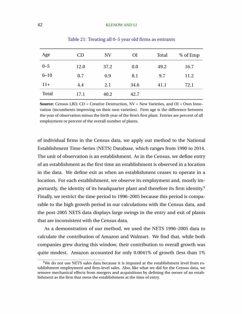
6.1. Treating all 0–5 year old firms as entrants

In Table 16, we show that new firms mostly contribute by introducing new vari-

eties, while young firms aged 1 to 5 contribute mostly through own-innovation.

In the presence of adjustment costs, however, what we infer as own innovation

by young firms may actually be the dynamics of accumulating inputs and ac-

quiring customers. We therefore check the robustness of our findings to treat-

ing age 1 to 5 firms as new firm. Doing so reinterprets the growth of young

firms to come from creative destruction and new varieties rather than own in-

novation. Table 21 displays the results. We find that new firms (aged 0 to 5) now

account for 49 percent of all growth, up from 30 percent. The contribution of

own innovation falls from 60 percent to 43 percent. That from creative destruc-

tion increases from 13 to 17 percent, while the contribution from new varieties

increases from 27 to 40 percent.

6.2. Contribution of superstar firms

One advantage of our method is that it can be used to quantify the contribu-

tion of individual firms to aggregate growth. Since we cannot reveal the identity

42 KLENOW AND LI

Table 21: Treating all 0–5 year old firms as entrants

Age CD NV OI Total % of Emp

0–5 12.0 37.2 0.0 49.2 16.7

6–10 0.7 0.9 8.1 9.7 11.2

11+ 4.4 2.1 34.6 41.1 72.1

Total 17.1 40.2 42.7

Source: Census LBD. CD = Creative Destruction, NV = New Varieties, and OI = Own Inno-

vation (incumbents improving on their own varieties). Firm age is the difference between

the year of observation minus the birth year of the firm’s first plant. Entries are percent of all

employment or percent of the overall number of plants.

of individual firms in the Census data, we apply our method to the National

Establishment Time-Series (NETS) Database, which ranges from 1990 to 2014.

The unit of observation is an establishment. As in the Census, we define entry

of an establishment as the first time an establishment is observed in a location

in the data. We define exit as when an establishment ceases to operate in a

location. For each establishment, we observe its employment and, mostly im-

portantly, the identity of its headquarter plant and therefore its firm identity.9

Finally, we restrict the time period to 1996–2005 because this period is compa-

rable to the high growth period in our calculations with the Census data, and

the post-2005 NETS data displays large swings in the entry and exit of plants

that are inconsistent with the Census data.

As a demonstration of our method, we used the NETS 1996–2005 data to

calculate the contribution of Amazon and Walmart. We find that, while both

companies grew during this window, their contribution to overall growth was

quite modest. Amazon accounted for only 0.0041% of growth (less than 1%

9We do not use NETS sales data because it is imputed at the establishment level from es-tablishment employment and firm-level sales. Also, like what we did for the Census data, weremove mechanical effects from mergers and acquisitions by defining the owner of an estab-lishment as the firm that owns the establishment at the time of entry.


of all growth), while Walmart contributed 0.80% (closer to 1% of all growth, or

over 2 basis points of annual TFP growth). Nonetheless, Amazon’s contribution

was three times its employment share, while Walmart’s growth contribution was

twice its employment share.

6.3. Future applications

Our innovation accounting is distinct from gross job creation, gross job destruc-

tion, or net job creation. It can therefore be helpful to contrast our results to

these statistics, which have garnered substantial attention. For example, young

fast-growing firms — so-called “gazelles” — are responsible for a notable frac-

tion of gross and net job creation. How much growth do they generate on aver-

age? And how much of gross job destruction is due to creative destruction, as

opposed to obsolescence?

We could carry out several important robustness checks. We could follow

Aghion, Bergeaud, Boppart, Klenow and Li (2019) and distinguish between mea-

sured and true growth. They argue that measured growth mostly captures own

innovation by incumbents, and misses most growth from new varieties and cre-

ative destruction. We could re-estimate parameters under this hypothesis.

For manufacturing the Census has data on revenue and capital as well as

labor at the plant level. Thus for manufacturing we could back out underlying

productivity, rather than assume sales are proportional to employment and the

absence of adjustment costs and distortions. We could apply our innovation

accounting on directly to this underlying productivity measure, and see how

our inference compares to that with employment alone.

Future work could implement our approach to assess the contribution of

locations (states, cities) to aggregate growth. It could also decompose growth

within industries such ICT or retail. One could also look at which cohorts of

entering firms have contributed the most to growth. Our method does not me-

chanically count firm employment growth due to mergers and acquisitions as

44 KLENOW AND LI

contributing to growth. But one could investigate whether targets of M&A activ-

ity become more innovative after they are taken over. This could obtain results

at odd with existing analyses, which focus on revenue productivity.

7. Conclusion

We exploited U.S. Census data on employment at plants across all firms in the

nonfarm business sector from 1982–2013. We traced aggregate TFP growth to

the innovation efforts of firms by their size and age. We arrived at three main

findings. First, young firms (ages 0 to 5) generate one-half of growth, roughly

three times more than their share of employment might suggest. Second, large

firms are at the other end of the spectrum, contributing notably less to growth

than their share of employment. Third, a majority of growth takes the form of

quality improvements by incumbents on their own products. New varieties and

creative destruction contribute less, but are still important. Such own innova-

tion accounts for the bulk of the growth speedup and slowdown in the middle

of our sample.

Our study comes with many caveats that we hope future work, with better

data, can address. We used a plant as a proxy for a product. With more de-

tailed data on products sold within plants, this can be relaxed. See, for exam-

ple, Bernard, Redding and Schott (2010) on manufacturing and Hottman et al.

(2016) on packaged consumer goods.

We gauged a plant’s size by its employment rather than its sales and com-

bined plants with a CES aggregator. Though they are highly correlated in man-

ufacturing, where we can see both, some innovation surely tilts toward capital

and away from labor (automation). And a richer analysis could place industries

into CES nests and entertain non-CES aggregation.

Even under CES aggregation, a plant’s sales are a perfect reflection of its un-

derlying productivity only in the absence of adjustment costs and distortions

such as markups, markdowns, and financial frictions. Adjustment costs could


include those for inputs, or to acquiring a customer base. We could be overstat-

ing the importance of young firms for innovation (overall and by incumbents on

their own products) if their fast growth is due, in part, to adjusting their inputs

and stock of customers.

We assumed that creative destruction was untargeted. That is, higher quality

products are just as likely to be creatively destroyed as lower quality products.

One can think of a priori reasons why creative destruction would target higher

quality products (more sales to gain) or lower quality products (perhaps easier

to improve upon).

We made the arrival rates and step sizes of innovation depend only on the

size and age of innovating firms . Studies such as Akcigit and Kerr (2018) have

argued that innovation by new and young firms generates bigger spillovers. This

would reinforce our conclusion that younger firms punch above their weight

class in terms of growth.

Our innovation accounting is silent on the determinants of arrival rates and

step sizes of innovation. Knowing the structural parameters that drive these

variables is vital for drawing policy lessons. See Atkeson and Burstein (2019).

One key question for future research is whether creative destruction is a strate-

gic complement or substitute for own innovation by incumbents. If they are

substitutes, as in Peters (2019) and Akcigit and Ates (2019), then a falling rate of

creative destruction may be offset by a rising rate of own innovation. If they are

complements, however, then perhaps the threat of creative destruction spurs

innovative efforts by incumbents. This is the spirit of the model in Aghion,

Bloom, Blundell, Griffith and Howitt (2005) in which the threat of being over-

taken by followers or entrants leads to more innovation by leaders.

46 KLENOW AND LI

8. Appendix with Extra Figures and Tables

Figure 3: Microsoft





Figure 4: Google




Figure 5: Facebook




48 KLENOW AND LI

Figure 6: Apple




Figure 7: Starbucks





Table 22: Obsolescence by age groups

Period Age % of Emp % of Plants contrib OB

1982–1995 0 0.0 0.0 0.0

1–5 2.1 5.8 -0.5

6–10 0.7 1.7 -0.2

11+ 1.3 2.9 -0.3

1996–2005 0 0.0 0.0 0.0

1–5 1.3 4.4 -0.1

6–10 0.5 1.4 -0.0

11+ 1.1 2.8 -0.1

2006–2013 0 0.0 0.0 0.0

1–5 1.5 4.6 -0.4

6–10 0.6 1.5 -0.2

11+ 0.8 2.9 -0.2

Source: Census LBD. Firm age is the difference between the year of observation minus the birth

year of the firm’s first plant. Units are percent of total employment or total number plants

50 KLENOW AND LI

Table 23: Obsolescence by size groups

Period Size % of Emp % of Plants contrib OB

1982–1995 0 0.0 0.0 0.0

1–19 2.6 9.2 -0.7

20–249 0.9 0.3 -0.2

250–999 0.1 0.1 -0.0

1k–4999 0.1 0.2 -0.0

5k–9999 0.1 0.1 -0.0

10k+ 0.4 0.4 -0.1

1996–2005 0 0.0 0.0 0.0

1–19 1.5 7.4 -0.2

20–249 0.6 0.2 -0.1

250–999 0.1 0.1 -0.0

1k–4999 0.1 0.2 -0.0

5k–9999 0.1 0.1 -0.0

10k+ 0.5 0.6 -0.0

2006–2013 0 0.0 0.0 0.0

1–19 2.0 8.3 -0.6

20–249 0.7 0.1 -0.2

250–999 0.0 0.0 0.0

1k–4999 0.0 0.1 0.0

5k–9999 0.0 0.1 0.0

10k+ 0.2 0.5 -0.0

Source: Census LBD. Firm size is the sum of employment across all of its plants. Units are percent

of total employment or total number plants


Table 24: Contribution by age-size groups, 1982–1995

Size Age CD NV OI Total % of Emp

0 0 7.6 30.3 0.0 37.9 3.9

1–19 1–5 0.1 0.7 16.4 17.1 7.2

1–19 6–10 0.3 0.4 6.1 6.8 4.2

1–19 11+ 0.4 0.0 10.4 10.8 7.7

20–249 1–5 0.0 1.1 2.2 3.4 5.6

20–249 6–10 0.0 0.8 1.3 2.1 4.6

20–249 11+ 0.1 1.6 4.4 6.1 15.5

250–999 1–5 0.3 0.0 0.0 0.3 1.3

250–999 6–10 0.2 0.0 0.0 0.2 1.4

250–999 11+ 0.1 0.0 2.5 2.6 9.3

1k–4999 1–5 0.2 0.0 0.0 0.2 0.9

1k–4999 6–10 0.4 0.0 0.2 0.6 1.1

1k–4999 11+ 0.6 0.1 2.6 3.4 11.5

5k–9999 1–5 0.2 0.0 0.0 0.2 0.5

5k–9999 6–10 0.2 0.0 0.0 0.2 0.3

5k–9999 11+ 0.4 0.0 0.7 1.2 5.1

10k+ 6–10 1.4 0.0 0.0 1.4 0.4

10k+ 11+ 3.5 0.2 1.7 5.4 19.5

Source: Census LBD. CD = Creative Destruction, NV = New Varieties, and OI = Own Innovation (in-cumbents improving on their own varieties). Firm size is the sum of employment across all of itsplants. Firm age is the difference between the year of observation minus the birth year of the firm’sfirst plant.

52 KLENOW AND LI



0 0 5.1 13.4 0.0 18.5 3.1

1–19 1–5 0.0 0.1 10.8 10.9 5.6

1–19 6–10 0.4 0.0 5.1 5.5 3.6

1–19 11+ 1.3 0.0 10.0 11.3 8.5

20–249 1–5 0.1 0.0 4.1 4.2 4.6

20–249 6–10 0.0 0.6 2.9 3.5 4.2

20–249 11+ 0.0 0.0 11.8 11.8 18.0

250–999 1–5 0.2 0.0 0.7 0.9 1.2

250–999 6–10 0.1 0.0 0.7 0.8 1.3

250–999 11+ 0.3 0.0 6.4 6.6 10.7

1k–4999 1–5 0.3 0.0 0.3 0.6 0.8

1k–4999 6–10 0.2 0.0 0.6 0.8 1.1

1k–4999 11+ 0.6 0.0 7.7 8.2 12.4

5k–9999 1–5 0.2 0.0 0.0 0.2 0.4

5k–9999 6–10 0.1 0.0 0.1 0.2 0.3

5k–9999 11+ 0.1 0.3 2.9 3.3 5.0

10k+ 6–10 0.2 0.0 0.2 0.4 0.5

10k+ 11+ 2.4 0.1 9.8 12.3 18.4

Source: Census LBD. CD = Creative Destruction, NV = New Varieties, and OI = Own Innovation (in-

cumbents improving on their own varieties). Firm size is the sum of employment across all of its

plants. Firm age is the difference between the year of observation minus the birth year of the firm’s

first plant.




0 0 8.9 21.2 0.0 30.1 2.5

1–19 1–5 0.0 0.2 12.6 12.8 4.8

1–19 6–10 0.2 0.0 5.2 5.4 3.2

1–19 11+ 2.1 0.0 11.1 13.2 9.0

20–249 1–5 0.0 0.9 2.4 3.3 4.0

20–249 6–10 0.1 0.4 1.8 2.3 3.7

20–249 11+ 0.0 2.5 6.6 9.1 18.6

250–999 1–5 0.0 0.0 0.3 0.3 1.0

250–999 6–10 0.1 0.0 0.5 0.6 1.2

250–999 11+ 0.0 1.8 4.5 6.3 11.2

1k–4999 1–5 0.1 0.0 0.0 0.1 0.6

1k–4999 6–10 0.1 0.0 0.4 0.4 0.9

1k–4999 11+ 0.2 0.0 5.9 6.2 13.6

5k–9999 1–5 0.0 0.0 0.0 0.0 0.3

5k–9999 6–10 0.1 0.0 0.0 0.1 0.2

5k–9999 11+ 0.1 0.0 2.5 2.6 5.3

10k+ 6–10 0.2 0.0 0.1 0.2 0.3

10k+ 11+ 0.5 0.1 6.3 6.9 19.6

Source: Census LBD. CD = Creative Destruction, NV = New Varieties, and OI = Own Innovation (in-

cumbents improving on their own varieties). Firm size is the sum of employment across all of its

plants. Firm age is the difference between the year of observation minus the birth year of the firm’s

first plant.

54 KLENOW AND LI

References

Acemoglu, Daron, “Labor- and Capital-Augmenting Technical Change,” Journal of the

European Economic Association, 2003, 1 (1), 1–37.

, Introduction to Modern Economic Growth, Princeton University Press, 2011.

Aghion, Philippe and Peter Howitt, “A Model of Growth Through Creative Destruction,”

Econometrica, 1992, 60 (2), 323–351.

and , The Economics of Growth, Massachusetts Institute of Technology (MIT)

Press, 2009.

, Antonin Bergeaud, Timo Boppart, Peter J. Klenow, and Huiyu Li, “Missing Growth

from Creative Destruction,” American Economic Review, 2019, 109 (8), 2795–2822.

, , , , and , “A Theory of Falling Growth and Rising Rents,” NBER Working

Paper 26448, 2020.

, Nick Bloom, Richard Blundell, Rachel Griffith, and Peter Howitt, “Competition and

Innovation: An Inverted-U Relationship,” Quarterly Journal of Economics, 2005, 120

(2), 701–728.

, Ufuk Akcigit, and Peter Howitt, “What Do We Learn from Schumpeterian Growth

Theory?,” Handbook of Economic Growth, 2014, 2, 515–563.

Akcigit, Ufuk and Sina T. Ates, “What Happened to U.S. Business Dynamism?,” NBER

Working Paper 25756, 2019.

and William R. Kerr, “Growth through Heterogeneous Innovations,” Journal of Polit-

ical Economy, 2018, 126 (4), 1374–1443.

Atkeson, Andrew and Ariel Burstein, “Aggregate Implications of Innovation Policy,”

Journal of Political Economy, 2019, 127 (6), 2625–2683.

Baily, Martin Neil, Charles Hulten, and David Campbell, “Productivity Dynamics in

Manufacturing Plants,” Brookings Papers: Microeconomics, 1992, 4, 187–267.


Baqaee, David Rezza and Emmanuel Farhi, “Productivity and Misallocation in General

Equilibrium,” Quarterly Journal of Economics, 2020, 135 (1), 105–163.

Bernard, Andrew B., Stephen J. Redding, and Peter K. Schott, “Multi-Product Firms and

Product Switching,” American Economic Review, 2010, 100 (1), 70–97.

Bloom, Nicholas, Charles I. Jones, John Van Reenen, and Michael Webb, “Are ideas get-

ting harder to find?,” NBER Working Paper 23782, 2017.

Broda, Christian and David E Weinstein, “Globalization and the Gains from Variety,”

Quarterly Journal of Economics, 2006, 121 (2), 541–585.

Decker, Ryan A., John Haltiwanger, Ron S. Jarmin, and Javier Miranda, “Declining Dy-

namism, Allocative Efficiency, and the Productivity Slowdown,” American Economic

Review, 2017, 107 (5), 322–26.

Decker, Ryan, John Haltiwanger, Ron Jarmin, and Javier Miranda, “The Role of En-

trepreneurship in U.S. Job Creation and Economic Dynamism,” Journal of Economic

Perspectives, 2014, 28 (3), 3–24.

Engbom, Niklas, “Firm and Worker Dynamics in an Aging Labor Market,” unpublished

paper, 2017.

Eslava, Marcela and John Haltiwanger, “The Life-Cycle Growth of Plants: The Role of

Productivity, Demand and Distortions,” unpublished paper, 2019.

Feenstra, Robert C., “New Product Varieties and the Measurement of International

Prices,” American Economic Review, 1994, 84 (1), 157–177.

Fernald, John G, “Productivity and Potential Output Before, During, and After the Great

Recession,” NBER Macroeconomics Annual, 2015, 29, 1–51.

Foster, Lucia, John C. Haltiwanger, and C.J. Krizan, “Aggregate Productivity Growth:

Lessons from Microeconomic Evidence,” New Developments in Productivity Analy-

sis, 2001, 8, 303–372.

56 KLENOW AND LI

, John Haltiwanger, and Chad Syverson, “Reallocation, Firm Turnover, and Efficiency:

Selection on Productivity or Profitability?,” American Economic Review, 2008, 98 (1),

394–425.

Garcia-Macia, Daniel, Chang-Tai Hsieh, and Peter J. Klenow, “How Destructive is Inno-

vation?,” Econometrica, 2019, 87 (5), 1507–1541.

Griliches, Zvi and Haim Regev, “Firm Productivity in Israeli Industry 1979–1988,” Jour-

nal of Econometrics, 1995, 65 (1), 175–203.

Gutierrez, German and Thomas Philippon, “Fading Stars,” AEA Papers and Proceedings,

2019, 109, 312–316.

Haltiwanger, John, Ron S. Jarmin, and Javier Miranda, “Who Creates Jobs? Small versus

Large versus Young,” Review of Economics and Statistics, 2013, 95 (2), 347–361.

Hopenhayn, Hugo A., “Entry, Exit, and Firm Dynamics in Long Run Equilibrium,”

Econometrica, 1992, 60 (5), 1127–1150.

Hopenhayn, Hugo, Julian Neira, and Rish Singhania, “From Population Growth to Firm

Demographics: Implications for Concentration, Entrepreneurship and the Labor

Share,” NBER Working Paper 25382, 2018.

Hottman, Colin J., Stephen J. Redding, and David E. Weinstein, “Quantifying the

Sources of Firm Heterogeneity,” Quarterly Journal of Economics, 2016, 131 (3), 1291–

1364.

Hsieh, Chang-Tai and Peter J. Klenow, “Misallocation and Manufacturing TFP in China

and India,” Quarterly Journal of Economics, 2009, 124 (4), 1403–1448.

and , “The Life Cycle of Plants in India and Mexico,” Quarterly Journal of Eco-

nomics, 2014, 129 (3), 1035–1084.

and , “The Reallocation Myth,” Fostering a Dynamic Global Economy, 2017.

, , and Ishan B. Nath, “A Global View of Creative Destruction,” NBER Working Paper

26461, 2019.


Jones, Charles I., “R&D-Based Models of Economic Growth,” Journal of Political Econ-

omy, 1995, 103 (4), 759–784.

, “Life and Growth,” Journal of Political Economy, 2016, 124 (2), 539–578.

Klette, Tor Jakob and Samuel Kortum, “Innovating Firms and Aggregate Innovation,”

Journal of Political Economy, 2004, 112 (5), 986–1018.

Krusell, Per, “How is R&D Distributed Across Firms? A Theoretical Analysis,” unpub-

lished paper, 1998.

Lentz, Rasmus and Dale T. Mortensen, “An Empirical Model of Growth through Product

Innovation,” Econometrica, 2008, 76 (6), 1317–1373.

Liu, Ernest, Atif Mian, and Amir Sufi, “Low Interest Rates, Market Power, and Produc-

tivity Growth,” NBER Working Paper 25505, 2019.

Lucas, Robert E. Jr. and Benjamin Moll, “Knowledge Growth and the Allocation of

Time,” Journal of Political Economy, 2014, 122 (1), 1–51.

Luttmer, Erzo G.J., “On the Mechanics of Firm Growth,” Review of Economic Studies,

2011, 78 (3), 1042–1068.

Mankiw, N. Gregory, David Romer, and David N. Weil, “A Contribution to the Empirics

of Economic Growth,” Quarterly Journal of Economics, 1992, 107 (2), 407–437.

Melitz, Marc J. and Saso Polanec, “Dynamic Olley-Pakes Productivity Decomposition

with Entry and Exit,” The RAND Journal of Economics, 2015, 46 (2), 362–375.

Olley, G. Steven and Ariel Pakes, “The Dynamics of Productivity in the Telecommuni-

cations Equipment Industry,” Econometrica, 1996, 64 (6), 1263–1297.

Peters, Michael, “Heterogeneous Mark-Ups, Growth and Endogenous Misallocation,”

forthcoming in Econometrica, 2019.

and Conor Walsh, “Declining Dynamism, Increasing Markups and Missing Growth:

The Role of the Labor Force,” unpublished paper, 2019.

58 KLENOW AND LI

Rivera-Batiz, Luis A. and Paul M. Romer, “Economic Integration and Endogenous

Growth,” Quarterly Journal of Economics, 1991, 106 (2), 531–555.

Romer, Paul M., “Endogenous Technological Change,” Journal of Political Economy,

1990, 98 (5, Part 2), S71–S102.

Solow, Robert M., “A Contribution to the Theory of Economic Growth,” Quarterly Jour-

nal of Economics, 1956, 70 (1), 65–94.

Documents

Innovative Growth AccountingINNOVATIVE GROWTH ACCOUNTING 3 We exploit ﬁrm and plant data on employment at all nonfarm businesses from 1983–2013 in the U.S. Census Bureau’s Longitudinal