lable at ScienceDirect

Renewable Energy 99 (2016) 602e613

Contents lists avai

Renewable Energy

journal homepage: www.elsevier .com/locate/renene

Influence of winter North-Atlantic Oscillation on Climate-Related-Energy penetration in Europe

B. François a, b, *

a Universit�e de Grenoble-Alpes, LTHE, 38041 Grenoble, Franceb CNRS, LTHE, 38041 Grenoble, France

a r t i c l e i n f o

Article history:Received 9 March 2016Received in revised form21 June 2016Accepted 7 July 2016

Keywords:Climate-Related EnergyPenetrationLow frequency variabilityNAO index

* Universit�e de Grenoble-Alpes, LTHE, 38041 GrenoE-mail address: baptistefrancois51@gmail.com.

http://dx.doi.org/10.1016/j.renene.2016.07.0100960-1481/© 2016 Elsevier Ltd. All rights reserved.

a b s t r a c t

When considering 100% renewable scenarios, backup generation is needed for stabilizing the networkwhen Climate Related Energy (CRE) such as wind, solar or run-of-the river hydropower are not sufficientfor supplying the load. Several studies show that, over relatively short time period (less than 10 years),backup generation needs are reduced by dissipating power densities either in space through grids ortime through storage. This study looks at the impact of low time frequency variations of CRE with aspecific focus on the time variability induced by the North Atlantic Oscillation (NAO) teleconnectionpattern during winter season. A set of eleven regions in Europe and Tunisia is used for highlighting spacevariability of the winter NAO’s impact. For each of these regions, we combine data from the WeatherResearch and Forecasting Model and the European Climate Assessment & Dataset for estimating solar-power, wind-power, run-of-the-river hydro-power and the energy load over the 1980e2012 timeperiod. Results show that NAO’s impact on winter penetration rate depends on both the consideredenergy source and the location. They also highlight a non-linear relation between the NAO’s impact onCRE penetration rates and the level of equipment used for harvesting the CRE sources.

© 2016 Elsevier Ltd. All rights reserved.

1. Introduction

The UNFCCC (United Nations Framework Convention on ClimateChange) Paris Agreement promotes the transition to low carboneconomy by replacing conventional energies by Climate-RelatedEnergies (hereafter called CRE) such as wind-power, solar-powerand hydro-power. Several European countries such as Norway,Sweden, Spain and Austria have already achieved an important stepforward to the transition with already a high rate of renewablegeneration [25]. The European Climate foundation now typicallydates for 2050 optimistic scenarios with close to 100% renewableenergy in Europe [4].

Following the driving weather variables (i.e. solar radiationwind speed, precipitation, and temperature), CRE power generationfluctuates in time and space and can synchronize or desynchronizewith the load [6]. With increasing rate of CRE equipment, balancingthe energy network requires solution of challenging backup gen-eration and energy storage issues due to the intermittent nature ofwind, solar and to a lesser extent, hydro-power [6]. Backup needs

ble, France.

must cover the wide range of time scales within which CRE drivingweather variables are fluctuating. The high frequency time vari-ability (i.e. from second to hour) is well known and quite welldocumented. For instance, wind and solar power generation mayexperience large and rapid variations, usually called ‘ramps’, linkedwith wind variability and cloud evolution and movement [5,13].This range of time variability may be handled by using fast rampingenergy storage technologies or backup generation (see for instance[12] for wind power balancing). The intermediate variability range(i.e. from hourly to seasonal) results from astronomic drivers (i.e.diurnal and seasonal cycles) and mesoscale atmospheric circula-tions (e.g. storms, fronts). Most of the published studies related tothis time range are based on relatively short time periods, usuallyshorter than ten years. These studies highlighted for instancedifferent degrees of complementarity among CREs at different timescales (e.g. Ref. [28] for solar andwind complementarity and Ref. [7]for solar and small hydro complementarity). They also discussedmethods for optimizing these complementarities (e.g. Ref. [18] foroptimizing solar and small hydro power complementarity), the roleof the energy grid (e.g. [35,19,30]); and the role of the energystorage (e.g. [35,29]).

Interestingly, low frequency time variability (from annual to

B. François / Renewable Energy 99 (2016) 602e613 603

decades) is less studied, although it plays a major role from thepoint of view of the equilibrium between energy generation andload. Assuming that CRE would be massively used to meet elec-tricity consumption, what is the risk of ending up in a situation inwhich the level of production of one or more CRE is exceptionallylow or exceptionally high for a long period of time and/or over alarge area? What would be the risk for an investor if the return oninvestment has been calculated on a high energy productionperiod? What would be the carbon emissions associated with themobilization of conventional means of production to compensatefor CRE in production resulting from a low-production period?Even though it might be partially explained by astronomic factors(e.g. solar activity cycle [26]); and geological events (e.g. volcanism;[31]), low frequency time variability results mainly from differentlarge-scale teleconnection patterns impacting the climate at globalscale (e.g. El Ni~no e Southern Oscillation (ENSO) in the tropics andin North America; the North Atlantic Oscillation (hereafter, NAO) inNorth America and Europe).

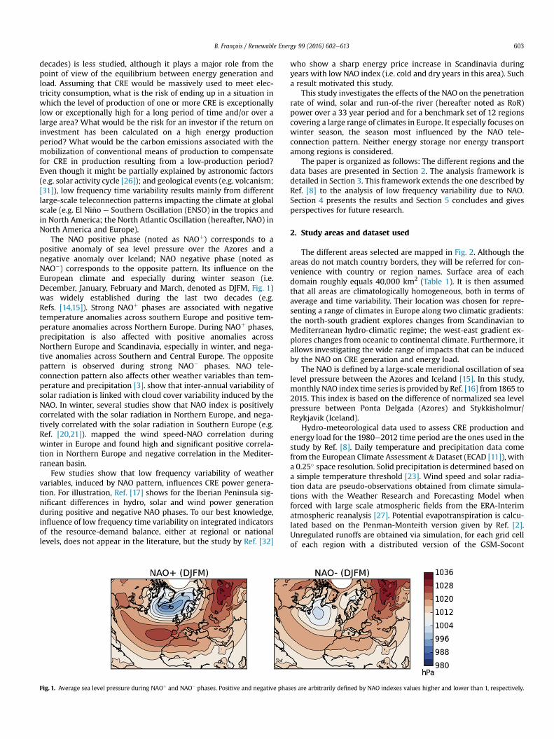
The NAO positive phase (noted as NAOþ) corresponds to apositive anomaly of sea level pressure over the Azores and anegative anomaly over Iceland; NAO negative phase (noted asNAO�) corresponds to the opposite pattern. Its influence on theEuropean climate and especially during winter season (i.e.December, January, February and March, denoted as DJFM, Fig. 1)was widely established during the last two decades (e.g.Refs. [14,15]). Strong NAOþ phases are associated with negativetemperature anomalies across southern Europe and positive tem-perature anomalies across Northern Europe. During NAOþ phases,precipitation is also affected with positive anomalies acrossNorthern Europe and Scandinavia, especially in winter, and nega-tive anomalies across Southern and Central Europe. The oppositepattern is observed during strong NAO� phases. NAO tele-connection pattern also affects other weather variables than tem-perature and precipitation [3]. show that inter-annual variability ofsolar radiation is linked with cloud cover variability induced by theNAO. In winter, several studies show that NAO index is positivelycorrelated with the solar radiation in Northern Europe, and nega-tively correlated with the solar radiation in Southern Europe (e.g.Ref. [20,21]). mapped the wind speed-NAO correlation duringwinter in Europe and found high and significant positive correla-tion in Northern Europe and negative correlation in the Mediter-ranean basin.

Few studies show that low frequency variability of weathervariables, induced by NAO pattern, influences CRE power genera-tion. For illustration, Ref. [17] shows for the Iberian Peninsula sig-nificant differences in hydro, solar and wind power generationduring positive and negative NAO phases. To our best knowledge,influence of low frequency time variability on integrated indicatorsof the resource-demand balance, either at regional or nationallevels, does not appear in the literature, but the study by Ref. [32]

Fig. 1. Average sea level pressure during NAOþ and NAO� phases. Positive and negative pha

who show a sharp energy price increase in Scandinavia duringyears with low NAO index (i.e. cold and dry years in this area). Sucha result motivated this study.

This study investigates the effects of the NAO on the penetrationrate of wind, solar and run-of-the river (hereafter noted as RoR)power over a 33 year period and for a benchmark set of 12 regionscovering a large range of climates in Europe. It especially focuses onwinter season, the season most influenced by the NAO tele-connection pattern. Neither energy storage nor energy transportamong regions is considered.

The paper is organized as follows: The different regions and thedata bases are presented in Section 2. The analysis framework isdetailed in Section 3. This framework extends the one described byRef. [8] to the analysis of low frequency variability due to NAO.Section 4 presents the results and Section 5 concludes and givesperspectives for future research.

2. Study areas and dataset used

The different areas selected are mapped in Fig. 2. Although theareas do not match country borders, they will be referred for con-venience with country or region names. Surface area of eachdomain roughly equals 40,000 km2 (Table 1). It is then assumedthat all areas are climatologically homogeneous, both in terms ofaverage and time variability. Their location was chosen for repre-senting a range of climates in Europe along two climatic gradients:the north-south gradient explores changes from Scandinavian toMediterranean hydro-climatic regime; the west-east gradient ex-plores changes from oceanic to continental climate. Furthermore, itallows investigating the wide range of impacts that can be inducedby the NAO on CRE generation and energy load.

The NAO is defined by a large-scale meridional oscillation of sealevel pressure between the Azores and Iceland [15]. In this study,monthly NAO index time series is provided by Ref. [16] from1865 to2015. This index is based on the difference of normalized sea levelpressure between Ponta Delgada (Azores) and Stykkisholmur/Reykjavik (Iceland).

Hydro-meteorological data used to assess CRE production andenergy load for the 1980e2012 time period are the ones used in thestudy by Ref. [8]. Daily temperature and precipitation data comefrom the European Climate Assessment& Dataset (ECAD [11]), witha 0.25� space resolution. Solid precipitation is determined based ona simple temperature threshold [23]. Wind speed and solar radia-tion data are pseudo-observations obtained from climate simula-tions with the Weather Research and Forecasting Model whenforced with large scale atmospheric fields from the ERA-Interimatmospheric reanalysis [27]. Potential evapotranspiration is calcu-lated based on the Penman-Monteith version given by Ref. [2].Unregulated runoffs are obtained via simulation, for each grid cellof each region with a distributed version of the GSM-Socont

ses are arbitrarily defined by NAO indexes values higher and lower than 1, respectively.

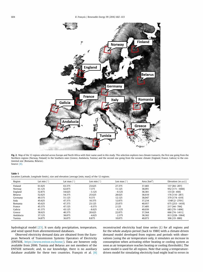
Fig. 2. Map of the 12 regions selected across Europe and North Africa with their name used in this study. This selection explores two climate transects, the first one going from theNorthern regions (Norway, Finland) to the Southern ones (Greece, Andalucía, Tunisia) and the second one going from the oceanic climate (England, France, Galicia) to the con-tinental one (Romania, Belarus).Source: [8].

Table 1Location (Latitude, Longitude limits), size and elevation (average [min, max]) of the 12 regions.

Region Lat min (�) Lat max (�) Lon min (�) Lon max (�) Area (km2) Elevation (m a.s.l.)

Finland 61.625 63.375 23.625 27.375 37,465 137 [84e207]Norway 61.125 62.875 7.375 11.125 38,091 952 [171e1660]England 52.875 54.625 �3.125 �0.125 38,381 133 [0e450]Belarus 52.625 54.375 25.625 28.625 38,610 176 [116e287]Germany 49.375 51.125 9.375 12.125 38,047 379 [174e619]Italy 45.625 47.375 10.375 12.875 37,234 1348 [2e2701]Romania 45.625 47.375 23.125 25.875 40,957 675 [253e1410]France 45.375 47.125 �0.375 2.125 37,405 217 [44e784]Galicia 41.375 43.125 �8.625 �6.125 40,039 683 [79e1496]Greece 38.625 40.375 20.625 22.875 37,564 666 [74e1411]Andalucia 37.125 38.875 �4.625 �2.375 38,362 813 [228e1964]Tunisia 34.875 36.875 8.875 10.875 40,073 306 [19e880]

B. François / Renewable Energy 99 (2016) 602e613604

hydrological model [23]. It uses daily precipitation, temperature,and wind speed from aforementioned databases.

Observed electricity demand data are obtained from the Euro-pean Network of Transmission Systems Operators of Electricity(ENTSOE, https://www.entsoe.eu/home/). Data are however onlyavailable from 2006. Tunisia and Belarus are not members of theENTSOE network; and, to our knowledge, there is no auxiliarydatabase available for these two countries. François et al. [8]

reconstructed electricity load time series (L) for all regions andfor the whole analysis period (back to 1980) with a climate-drivendemand model developed from regions and periods with obser-vations (using the air temperature only, it simulates an increase inconsumption when activating either heating or cooling system assoon as air temperature reaches heating or cooling thresholds). Thesame model is used for all regions. Note that using a temperature-driven model for simulating electricity load might lead to errors in

B. François / Renewable Energy 99 (2016) 602e613 605

some regions, especially where heating is mainly based on gas orbiomass burning. In such as case, the energy consumption sea-sonality should be weak and should result to an almost constantconsumption during the whole year. However, as pointed byRef. [8]; such a misestimate should not alter the interpretationsmade in this study since CRE generation time variability is muchhigher than load time variability.

Solar, wind and RoR power generation are computed for eachgrid cell of ECAD reanalysis data set and are then summed for eachregion [8]. The data bases used for modeling power generationfrom each energy source are the aforementioned weather variablesafter being re-meshed to ECAD grid. For the sake of simplicity, allgrid cells have the same power capacity. Solar power generationfrom a photovoltaic generator (PPV) depends on global solar irra-diance and air temperature. Daily wind power generation (PW) isobtained from mean daily wind speed at 70 m altitude. The windpower curve used for converting wind speed towind-power outputwas obtained by taking into account wind speed variability at 3 htime step [8]. RoR power (PRoR) is derived from the energy of fallingwater along the river network.

3. Study framework

The study framework used in this study extends the oneestablished by Ref. [8] to the analysis of low frequency variabilityrelated to the NAO pattern. Each region is considered as autono-mous in a sense that the regional demand can be only satisfied (ornot) with the production obtained within the region from thesethree energy sources: there is no energy import/export withneighboring regions. Furthermore, each region is considered asbeing a ‘copper plate’ grid, meaning that the energy can circulatewithin the regions without loses. For each energy source and eachregion, we explore equipment scenarios covering from 0 to 300% ofthe average energy load. For a given equipment level, power gen-eration time series are obtained following the equation:

pðt;gÞ ¼ gPðtÞ⟨PðtÞ⟩ ⟨LðtÞ⟩; (1)

with P the energy generation from one energy source in a givenregion (Wh), L the in situ energy load (Wh) and p the scaled energyproduction (Wh). ⟨⟩ is the temporal mean operator. The factor g (nodimension), further referred to as the average CRE productionfactor, corresponds to the level of CRE equipment. This coefficientallows exploring scenarios of under- (respectively over-) produc-tion by defining the ratio between generation and load over theconsidered period:

⟨pðt;gÞ⟩ ¼ g ⟨LðtÞ⟩: (2)

It equals 1 when the mean energy production fits the meanenergy load over the 1980e2012 time period. It is greater than 1when the mean inter-annual production exceeds the mean inter-annual load and conversely.

The penetration rate over the 1980e2012 time period is definedas the percentage of the energy load that is instantaneously sup-plied without any storage or backup facilities. For a given value ofthe average CRE generation factor g, the penetration rate PE (%) isestimated from daily time series by:

PEðgÞ ¼�1�

Ptðmax½LðtÞ � pðt;gÞ;0�ÞP

tLðtÞ�� 100; (3)

where max [ ] is the maximum operator. In the following, thepenetration function will refer to the function PE (g). It is definedwith penetration rates obtained for average CRE generation factor g

ranging from 0 to 3. For illustration, Fig. 3 gives penetration func-tions of solar, wind and RoR power for England, Belarus, Germanyand Andalucía regions over 1980e2012 period. Increasing averageCRE generation factor along the x-axis may be seen as increasinglevel of CRE equipment throughout energy transition process, i.e.moving from 0% of CRE power generation to a generation equal to300% of the energy load, on average and over the studied period.For a given level of equipment g, the penetration rate indicator mayintegrate interactions between generation and load which cannotbe highlighted when focusing only on generation. For the fourillustrated regions, for instance, Fig. 3 shows that penetration ratesdo not differ from one energy source to another up to g ¼ 0.4meaning that, i) whatever the chosen CRE for supplying the energyload, the penetration is the same, and that ii) linear relation be-tween penetration and load exists at these equipment levels (seeFig. 4). This linear relation exists as long as the power generationdoes not exceed the load at any time [29]. Above this threshold,François et al. [8] show that for a given energy source (and even agiven energy mix), the higher the energy balance variability(defined as the energy load e energy generation deviations), thelower the penetration rate; in some cases, significant correlation(or anti-correlation) between load and generation can slightlymodulate this relation. This turns into non-linear relation betweenpenetration rate and generation. For illustration Fig. 4 shows, forFinland region, that annual penetration rates obtained for differentyears with similar annual power generation can be significantlydistinct. This means that energy abundancy does not necessarilytranslate into high penetration rate. In that sense, focusing on anintegrated indicator of the energy balance such as the penetrationrate, rather than only a power generation indicator, is a step for-ward to better understanding how CREmight be used for supplyingelectricity needs.

In this study, we focus on the inter-annual variability of thepenetration rates during the DJFM season and its connection withthe NAO pattern. Note that the DJFM season is defined as Decemberduring the year k-1 and January, February and March during theyear k. In the following, penetration functions are estimated duringthe DJFM season for each year of the studied period. It thus givesthe percentage of satisfied load during the DJFM season for a givenyear k, hereafter noted as PEDJFM,k:

PEDJFM;kðgÞ ¼"1�

Pt2DJFM;kðmax½LðtÞ � pðt;gÞ;0�ÞP

t2DJFM;kðLðtÞÞ

#� 100;

(4)

with year k ranging from 1981 to 2012. Further, the averageDJFM penetration function, referred as PEDJFM(g), is simply definedas the mean of the PEDJFM,k(g) functions. Annual differences be-tween DJFM penetration rates are further discussed in terms ofanomalies, hereafter noted as DPEDJFM,k. They are obtained bysubtracting the average DJFM penetration function PEDJFM(g) fromthe DJFM penetration functions PEDJFM,k(g):

DPEDJFM;kðgÞ ¼ PEDJFM;kðgÞ � PEDJFMðgÞ; (5)

For a given year k, high positive or negative penetrationanomalies indicate important energy transport operations andbackup generation (i.e. in case of negative anomalies) or storageoperations and generation curtailment by disconnecting powerplants from the grid (i.e. in case of positive anomalies). Both optionsmay induce important extra management costs. Further, largeDPEDJFM,k(g) values, either positive or negative, will be considered aproxy for system vulnerability to low-frequency variability inducedby the NAO teleconnection pattern.

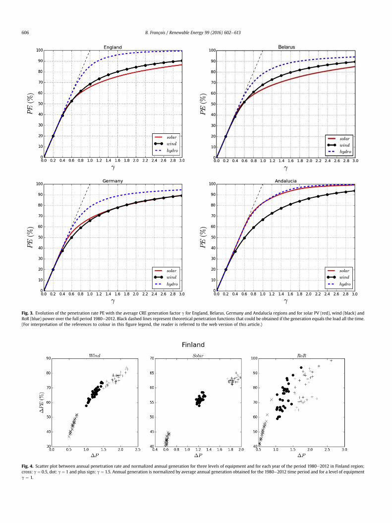
Fig. 3. Evolution of the penetration rate PE with the average CRE generation factor g for England, Belarus, Germany and Andalucía regions and for solar PV (red), wind (black) andRoR (blue) power over the full period 1980e2012. Black dashed lines represent theoretical penetration functions that could be obtained if the generation equals the load all the time.(For interpretation of the references to colour in this figure legend, the reader is referred to the web version of this article.)

Fig. 4. Scatter plot between annual penetration rate and normalized annual generation for three levels of equipment and for each year of the period 1980e2012 in Finland region;cross: g ¼ 0.5, dot: g ¼ 1 and plus sign: g ¼ 1.5. Annual generation is normalized by average annual generation obtained for the 1980e2012 time period and for a level of equipmentg ¼ 1.

B. François / Renewable Energy 99 (2016) 602e613606

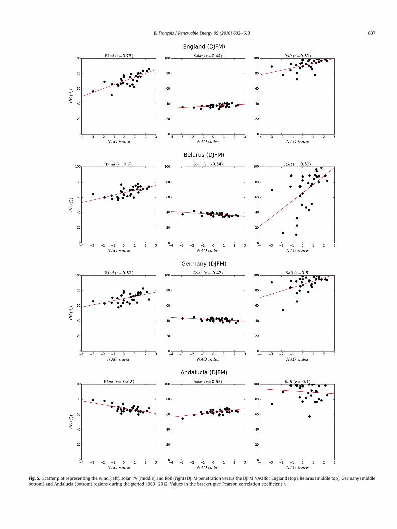
Fig. 5. Scatter plot representing the wind (left), solar PV (middle) and RoR (right) DJFM penetration versus the DJFM NAO for England (top), Belarus (middle top), Germany (middlebottom) and Andalucía (bottom) regions during the period 1980e2012. Values in the bracket give Pearson correlation coefficient r.

B. François / Renewable Energy 99 (2016) 602e613 607

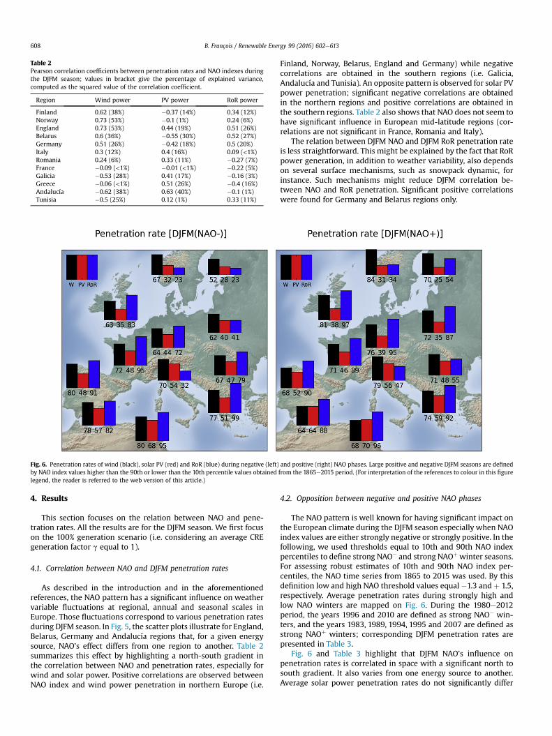
Table 2Pearson correlation coefficients between penetration rates and NAO indexes duringthe DJFM season; values in bracket give the percentage of explained variance,computed as the squared value of the correlation coefficient.

Region Wind power PV power RoR power

Finland 0.62 (38%) �0.37 (14%) 0.34 (12%)Norway 0.73 (53%) �0.1 (1%) 0.24 (6%)England 0.73 (53%) 0.44 (19%) 0.51 (26%)Belarus 0.6 (36%) �0.55 (30%) 0.52 (27%)Germany 0.51 (26%) �0.42 (18%) 0.5 (20%)Italy 0.3 (12%) 0.4 (16%) 0.09 (<1%)Romania 0.24 (6%) 0.33 (11%) �0.27 (7%)France �0.09 (<1%) �0.01 (<1%) �0.22 (5%)Galicia �0.53 (28%) 0.41 (17%) �0.16 (3%)Greece �0.06 (<1%) 0.51 (26%) �0.4 (16%)Andalucía �0.62 (38%) 0.63 (40%) �0.1 (1%)Tunisia �0.5 (25%) 0.12 (1%) 0.33 (11%)

Fig. 6. Penetration rates of wind (black), solar PV (red) and RoR (blue) during negative (left) and positive (right) NAO phases. Large positive and negative DJFM seasons are definedby NAO index values higher than the 90th or lower than the 10th percentile values obtained from the 1865e2015 period. (For interpretation of the references to colour in this figurelegend, the reader is referred to the web version of this article.)

B. François / Renewable Energy 99 (2016) 602e613608

4. Results

This section focuses on the relation between NAO and pene-tration rates. All the results are for the DJFM season. We first focuson the 100% generation scenario (i.e. considering an average CREgeneration factor g equal to 1).

4.1. Correlation between NAO and DJFM penetration rates

As described in the introduction and in the aforementionedreferences, the NAO pattern has a significant influence on weathervariable fluctuations at regional, annual and seasonal scales inEurope. Those fluctuations correspond to various penetration ratesduring DJFM season. In Fig. 5, the scatter plots illustrate for England,Belarus, Germany and Andalucía regions that, for a given energysource, NAO’s effect differs from one region to another. Table 2summarizes this effect by highlighting a north-south gradient inthe correlation between NAO and penetration rates, especially forwind and solar power. Positive correlations are observed betweenNAO index and wind power penetration in northern Europe (i.e.

Finland, Norway, Belarus, England and Germany) while negativecorrelations are obtained in the southern regions (i.e. Galicia,Andalucía and Tunisia). An opposite pattern is observed for solar PVpower penetration; significant negative correlations are obtainedin the northern regions and positive correlations are obtained inthe southern regions. Table 2 also shows that NAO does not seem tohave significant influence in European mid-latitude regions (cor-relations are not significant in France, Romania and Italy).

The relation between DJFM NAO and DJFM RoR penetration rateis less straightforward. This might be explained by the fact that RoRpower generation, in addition to weather variability, also dependson several surface mechanisms, such as snowpack dynamic, forinstance. Such mechanisms might reduce DJFM correlation be-tween NAO and RoR penetration. Significant positive correlationswere found for Germany and Belarus regions only.

4.2. Opposition between negative and positive NAO phases

The NAO pattern is well known for having significant impact onthe European climate during the DJFM season especially when NAOindex values are either strongly negative or strongly positive. In thefollowing, we used thresholds equal to 10th and 90th NAO indexpercentiles to define strong NAO� and strong NAOþ winter seasons.For assessing robust estimates of 10th and 90th NAO index per-centiles, the NAO time series from 1865 to 2015 was used. By thisdefinition low and high NAO threshold values equal �1.3 and þ 1.5,respectively. Average penetration rates during strongly high andlow NAO winters are mapped on Fig. 6. During the 1980e2012period, the years 1996 and 2010 are defined as strong NAO� win-ters, and the years 1983, 1989, 1994, 1995 and 2007 are defined asstrong NAOþ winters; corresponding DJFM penetration rates arepresented in Table 3.

Fig. 6 and Table 3 highlight that DJFM NAO’s influence onpenetration rates is correlated in space with a significant north tosouth gradient. It also varies from one energy source to another.Average solar power penetration rates do not significantly differ

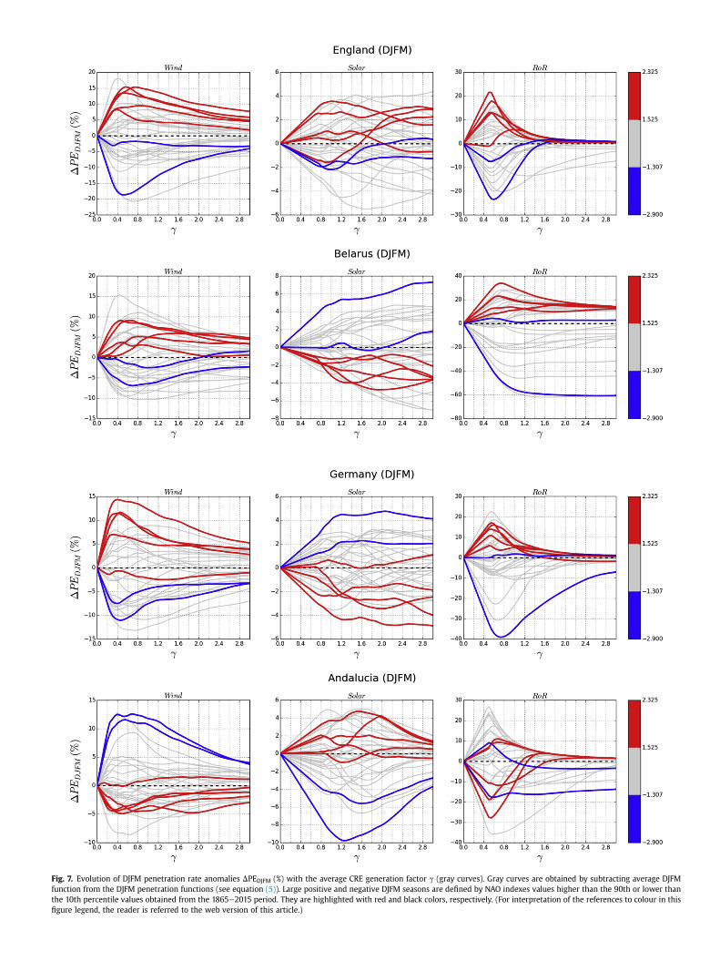
Fig. 7. Evolution of DJFM penetration rate anomalies DPEDJFM (%) with the average CRE generation factor g (gray curves). Gray curves are obtained by subtracting average DJFMfunction from the DJFM penetration functions (see equation (5)). Large positive and negative DJFM seasons are defined by NAO indexes values higher than the 90th or lower thanthe 10th percentile values obtained from the 1865e2015 period. They are highlighted with red and black colors, respectively. (For interpretation of the references to colour in thisfigure legend, the reader is referred to the web version of this article.)

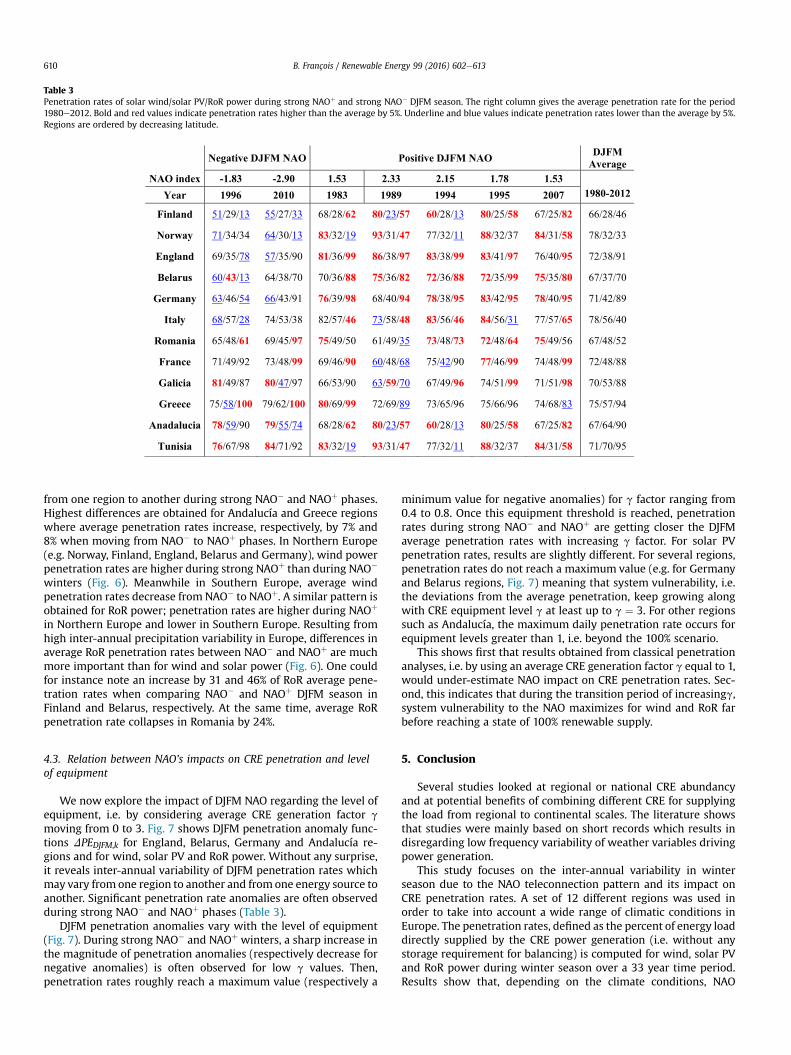
Table 3Penetration rates of solar wind/solar PV/RoR power during strong NAOþ and strong NAO� DJFM season. The right column gives the average penetration rate for the period1980e2012. Bold and red values indicate penetration rates higher than the average by 5%. Underline and blue values indicate penetration rates lower than the average by 5%.Regions are ordered by decreasing latitude.

B. François / Renewable Energy 99 (2016) 602e613610

from one region to another during strong NAO� and NAOþ phases.Highest differences are obtained for Andalucía and Greece regionswhere average penetration rates increase, respectively, by 7% and8% when moving from NAO� to NAOþ phases. In Northern Europe(e.g. Norway, Finland, England, Belarus and Germany), wind powerpenetration rates are higher during strong NAOþ than during NAO�

winters (Fig. 6). Meanwhile in Southern Europe, average windpenetration rates decrease from NAO� to NAOþ. A similar pattern isobtained for RoR power; penetration rates are higher during NAOþ

in Northern Europe and lower in Southern Europe. Resulting fromhigh inter-annual precipitation variability in Europe, differences inaverage RoR penetration rates between NAO� and NAOþ are muchmore important than for wind and solar power (Fig. 6). One couldfor instance note an increase by 31 and 46% of RoR average pene-tration rates when comparing NAO� and NAOþ DJFM season inFinland and Belarus, respectively. At the same time, average RoRpenetration rate collapses in Romania by 24%.

4.3. Relation between NAO’s impacts on CRE penetration and levelof equipment

We now explore the impact of DJFM NAO regarding the level ofequipment, i.e. by considering average CRE generation factor g

moving from 0 to 3. Fig. 7 shows DJFM penetration anomaly func-tions DPEDJFM,k for England, Belarus, Germany and Andalucía re-gions and for wind, solar PV and RoR power. Without any surprise,it reveals inter-annual variability of DJFM penetration rates whichmay vary from one region to another and from one energy source toanother. Significant penetration rate anomalies are often observedduring strong NAO� and NAOþ phases (Table 3).

DJFM penetration anomalies vary with the level of equipment(Fig. 7). During strong NAO� and NAOþ winters, a sharp increase inthe magnitude of penetration anomalies (respectively decrease fornegative anomalies) is often observed for low g values. Then,penetration rates roughly reach a maximum value (respectively a

minimum value for negative anomalies) for g factor ranging from0.4 to 0.8. Once this equipment threshold is reached, penetrationrates during strong NAO� and NAOþ are getting closer the DJFMaverage penetration rates with increasing g factor. For solar PVpenetration rates, results are slightly different. For several regions,penetration rates do not reach a maximum value (e.g. for Germanyand Belarus regions, Fig. 7) meaning that system vulnerability, i.e.the deviations from the average penetration, keep growing alongwith CRE equipment level g at least up to g ¼ 3. For other regionssuch as Andalucía, the maximum daily penetration rate occurs forequipment levels greater than 1, i.e. beyond the 100% scenario.

This shows first that results obtained from classical penetrationanalyses, i.e. by using an average CRE generation factor g equal to 1,would under-estimate NAO impact on CRE penetration rates. Sec-ond, this indicates that during the transition period of increasingg,system vulnerability to the NAO maximizes for wind and RoR farbefore reaching a state of 100% renewable supply.

5. Conclusion

Several studies looked at regional or national CRE abundancyand at potential benefits of combining different CRE for supplyingthe load from regional to continental scales. The literature showsthat studies were mainly based on short records which results indisregarding low frequency variability of weather variables drivingpower generation.

This study focuses on the inter-annual variability in winterseason due to the NAO teleconnection pattern and its impact onCRE penetration rates. A set of 12 different regions was used inorder to take into account a wide range of climatic conditions inEurope. The penetration rates, defined as the percent of energy loaddirectly supplied by the CRE power generation (i.e. without anystorage requirement for balancing) is computed for wind, solar PVand RoR power during winter season over a 33 year time period.Results show that, depending on the climate conditions, NAO

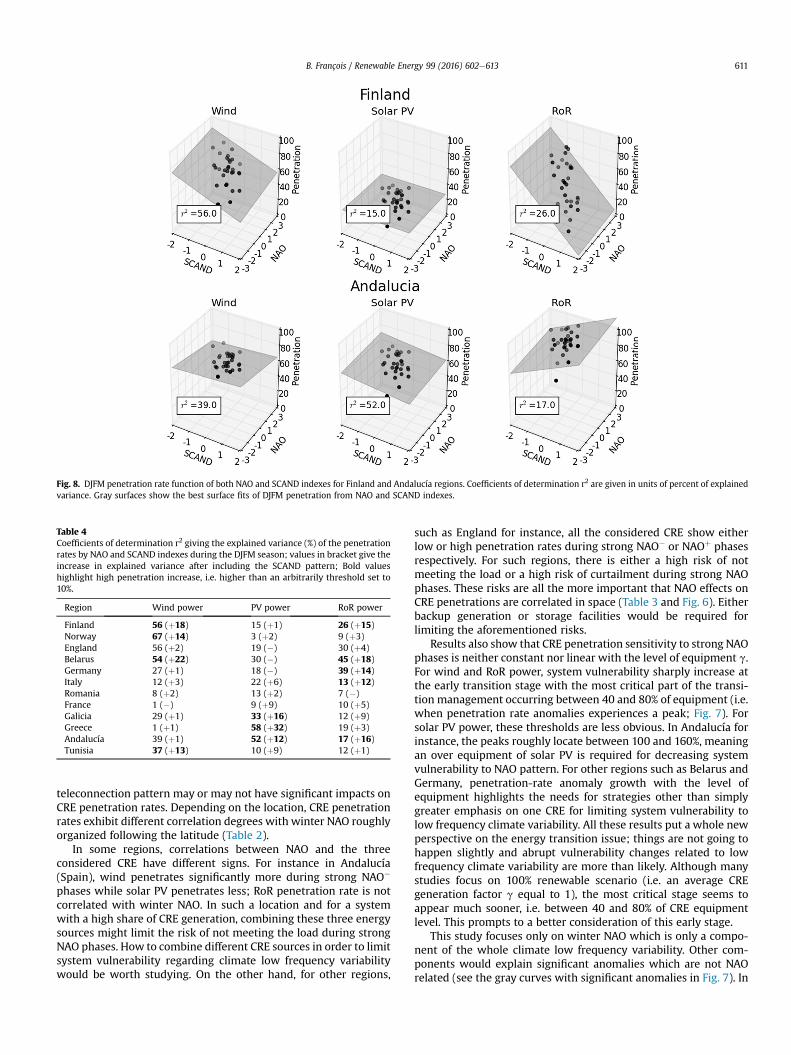
Fig. 8. DJFM penetration rate function of both NAO and SCAND indexes for Finland and Andalucía regions. Coefficients of determination r2 are given in units of percent of explainedvariance. Gray surfaces show the best surface fits of DJFM penetration from NAO and SCAND indexes.

Table 4Coefficients of determination r2 giving the explained variance (%) of the penetrationrates by NAO and SCAND indexes during the DJFM season; values in bracket give theincrease in explained variance after including the SCAND pattern; Bold valueshighlight high penetration increase, i.e. higher than an arbitrarily threshold set to10%.

Region Wind power PV power RoR power

Finland 56 (þ18) 15 (þ1) 26 (þ15)Norway 67 (þ14) 3 (þ2) 9 (þ3)England 56 (þ2) 19 (�) 30 (þ4)Belarus 54 (þ22) 30 (�) 45 (þ18)Germany 27 (þ1) 18 (�) 39 (þ14)Italy 12 (þ3) 22 (þ6) 13 (þ12)Romania 8 (þ2) 13 (þ2) 7 (�)France 1 (�) 9 (þ9) 10 (þ5)Galicia 29 (þ1) 33 (þ16) 12 (þ9)Greece 1 (þ1) 58 (þ32) 19 (þ3)Andalucía 39 (þ1) 52 (þ12) 17 (þ16)Tunisia 37 (þ13) 10 (þ9) 12 (þ1)

B. François / Renewable Energy 99 (2016) 602e613 611

teleconnection pattern may or may not have significant impacts onCRE penetration rates. Depending on the location, CRE penetrationrates exhibit different correlation degrees with winter NAO roughlyorganized following the latitude (Table 2).

In some regions, correlations between NAO and the threeconsidered CRE have different signs. For instance in Andalucía(Spain), wind penetrates significantly more during strong NAO�

phases while solar PV penetrates less; RoR penetration rate is notcorrelated with winter NAO. In such a location and for a systemwith a high share of CRE generation, combining these three energysources might limit the risk of not meeting the load during strongNAO phases. How to combine different CRE sources in order to limitsystem vulnerability regarding climate low frequency variabilitywould be worth studying. On the other hand, for other regions,

such as England for instance, all the considered CRE show eitherlow or high penetration rates during strong NAO� or NAOþ phasesrespectively. For such regions, there is either a high risk of notmeeting the load or a high risk of curtailment during strong NAOphases. These risks are all the more important that NAO effects onCRE penetrations are correlated in space (Table 3 and Fig. 6). Eitherbackup generation or storage facilities would be required forlimiting the aforementioned risks.

Results also show that CRE penetration sensitivity to strong NAOphases is neither constant nor linear with the level of equipment g.For wind and RoR power, system vulnerability sharply increase atthe early transition stage with the most critical part of the transi-tion management occurring between 40 and 80% of equipment (i.e.when penetration rate anomalies experiences a peak; Fig. 7). Forsolar PV power, these thresholds are less obvious. In Andalucía forinstance, the peaks roughly locate between 100 and 160%, meaningan over equipment of solar PV is required for decreasing systemvulnerability to NAO pattern. For other regions such as Belarus andGermany, penetration-rate anomaly growth with the level ofequipment highlights the needs for strategies other than simplygreater emphasis on one CRE for limiting system vulnerability tolow frequency climate variability. All these results put a whole newperspective on the energy transition issue; things are not going tohappen slightly and abrupt vulnerability changes related to lowfrequency climate variability are more than likely. Although manystudies focus on 100% renewable scenario (i.e. an average CREgeneration factor g equal to 1), the most critical stage seems toappear much sooner, i.e. between 40 and 80% of CRE equipmentlevel. This prompts to a better consideration of this early stage.

This study focuses only on winter NAO which is only a compo-nent of the whole climate low frequency variability. Other com-ponents would explain significant anomalies which are not NAOrelated (see the gray curves with significant anomalies in Fig. 7). In

B. François / Renewable Energy 99 (2016) 602e613612

Europe, several other teleconnection patterns were identifiedduring the last decades, and some of themwould deserve attention,such as the Scandinavia pattern (noted as SCAND, it was previouslyreferred as Eurasia-1 pattern; [1]). Its positive phase is associatedwith positive height anomalies over Scandinavia and westernRussia, while the negative phase is associated with negative heightanomalies in these regions. For illustration only, Fig. 8 shows pre-liminary results highlighting multivariate linear regressions of CREpenetration rates from NAO and SCAND indexes. Depending onclimate context, considering SCAND pattern in addition to NAOpattern allows better explanation of the penetration rates. In-creases in explained variances are reported on Table 4. Futureworks should extend this analysis to other climate patterns in orderto better understand the relation between CRE penetration andclimate variability.

Presented results and discussed interpretations therefore needto be validated over a longer time period. Indeed, as discussed byRef. [9]; taking into account the long payback periods of CRE gen-eration and storage technologies, a long term perspective isnecessary. A succession of either strong NAOþ or NAO� and theirimpact on CRE penetration must be investigated in future works(see for instance consecutive 1994 and 1995 years with strongwinter NAO� phases). Such a study could for instance benefits ofthe new large-scale reanalysis data [33,34]. Such large scale studiesshould motivate to prospective analyses related to seasonal todecadal predictions of the winter NAO [22,24]. These studies couldeventually help stakeholders for planning energy transport, storageand backup generation operations for reducing vulnerabilityrelated to low-frequency weather variability.

Finally, by considering that all the grid cells have the same po-wer capacity, this study only focuses on the weather component ofthe system vulnerability. Taking into account land-use and orog-raphy constraints might lead to a more realistic assessment ofsystem vulnerability related to low-frequency induced by tele-connections patterns. For instance Hansen and Thorn [10] mappedthe share of land area available for solar PV-panel installations inEurope. They show that some of the considered regions are notsuitable for solar PV installations (e.g. Finland and Greece). For suchregions, this implies that high CRE equipment levels g are notrealistic. Future researches should take into account this point forthe vulnerability assessment.

Acknowledgements

This work is part of the FP7 project COMPLEX (Knowledge basedclimate mitigation systems for a low carbon economy; Project FP7-ENV-2012 number: 308601; http://www.complex.ac.uk/). This pa-per also benefited from comments and suggestions from twoanonymous reviewers.

References

[1] A. Barnston, R.E. Livezey, Classification, seasonality and persistence of low-frequency atmospheric circulation patterns, Mon. Weather Rev. 115 (1987)1083e1126.

[2] R. Burman, L.O. Pochop, Evaporation, Evapotranspiration and Climatic Data,Elsevier, Amsterdam, 1994, 278pp.

[3] M. Chiacchio, M. Wild, Influence of NAO and clouds on long-term seasonalvariations of surface solar radiation in Europe, J. Geophys. Res. 115 (2010)D00D22, http://dx.doi.org/10.1029/2009JD012182.

[4] ECF, Roadmap 2050: a practical guide to a prosperous, low-carbon Europe,Eur. Clim. Found. 1 (2010) 100. Available online: http://www.roadmap2050.eu/. Last access November 2014.

[5] N. Francis, Predicting sudden changes in wind power generation, North Am.Wind 5 (2008) 58e60.

[6] B. François, M. Borga, S. Anquetin, J.D. Creutin, K. Engeland, A.C. Favre,B. Hingray, M.H. Ramos, D. Raynaud, B. Renard, E. Sauquet, J.F. Sauterleute,J.P. Vidal, G. Warland, Integrating hydropower and intermittent climate-related renewable energies: a call for hydrology, Hydrol. Process 28 (2014)

5465e5468.[7] B. François, M. Borga, J.D. Creutin, B. Hingray, D. Raynaud, J.F. Sauterleute,

Complementarity between solar and hydro power: sensitivity study to climatecharacteristics in Northern-Italy, Renew. Energy 86 (2016a) 543e553, http://dx.doi.org/10.1016/j.renene.2015.08.044.

[8] B. François, B. Hingray, D. Raynaud, M. Borga, J.D. Creutin, Increasing climate-related-energy penetration by integrating run-of-the river hydropower towind/solar mix, Renew. Energy 87 (2016b) 686e696.

[9] L. Gaudard, J. Gabbi, A. Bauder, F. Romerio, Long-term uncertainty of hydro-power revenue due to climate change and electricity prices, Water Resour.Manag. 30 (2016) 1325e1343.

[10] A.C. Hansen, P. Thorn, PV Potential and Potential PV Rent in European Regions,Roskilde University, Denmark, 2013. Tech. Report. Available at: http://rossy.ruc.dk/ojs/index.php/grec/article/view/3059/1322. Last access: June 2016.

[11] M.R. Haylock, N. Hofstra, A.M.G. Klein Tank, E.J. Klok, P.D. Jones, M. New,A European daily high-resolution gridded data set of surface temperature andprecipitation for 1950e2006, J. Geophys. Res. 113 (2008) D20119, http://dx.doi.org/10.1029/2008JD010201.

[12] E. Hittinger, J. Whitacre, J. Apt, Compensating for wind variability using co-located natural gas generation and energy storage, Energy Syst. 1 (4) (2010)417, http://dx.doi.org/10.1007/s12667-010-0017-2.

[13] T.E. Hoff, R. Perez, Quantifying PV power output variability, Sol. Energy 84(2010) 1782e1793.

[14] J.W. Hurrell, H. van Loon, Decadal variations in climate associated with theNorth Atlantic Oscillation, Clim. Change 36 (1997) 301e326.

[15] J.W. Hurrell, Decadal trends in the North Atlantic Oscillation: regional tem-peratures and precipitation, Science 269 (1995) 676e679.

[16] Hurrell, NAO Index Data provided by the Climate Analysis Section, NCAR,Boulder, USA, 2003. Available online: https://climatedataguide.ucar.edu/climate-data/hurrell-north-atlantic-oscillation-nao-index-station-based(Accessed 01/01/2016).

[17] S. Jerez, R.M. Trigo, S.M. Vicente-Serrano, D. Pozo-V�azquez, R. Lorente-Plazas,J. Lorenzo-Lacruz, F. Santos-Alamillos, J.P. Mont�avez, The impact of the NorthAtlantic Oscillation on renewable energy resources in Southwestern Europe,J. Appl. Meteorol. Climatol. 52 (2013) 2204e2225.

[18] I. Kougias, S. Szab�o, F. Monforti-Ferrario, T. Huld, K. B�odis, A methodology foroptimization of the complementarity between small-hydropower plants andsolar PV systems, Renew. Energy 87 (2015) 1023e1030.

[19] A.E. MacDonald, C.T.M. Clack, A. Alexander, A. Dunbar, J. Wilczak, Y. Xie,Future cost-competitive electricity systems and their impact on US CO2emissions, Nat. Clim. Change 6 (2016) 526e531.

[20] D. Pozo-V�azquez, J. Tovar-Pescador, S.R. G�amiz-Fortis, M.J. Esteban-Parra,Y. Castro-Díez, NAO and solar radiation variability in the European NorthAtlantic region, Geophys. Res. Lett. 31 (2004) L05201.

[21] D. Pozo-V�azquez, F.J. Santos-Alamillos, V. Lara-Fanego, J.A. Ruiz-Arias, J. Tovar-Pescador, The impact of the NAO on the solar and wind energy resources inthe Mediterranean area, in: S.M. Vicente-Serrano, R.M. Trigo (Eds.), Advancesin Global Change Research: Hydrological, Socio-economic and Ecological Im-pacts of the North Atlantic Oscillation in the Mediterranean Region, Springer,2011, pp. 213e231.

[22] A.A. Scaife, A. Arribas, E. Blockley, A. Brookshaw, R.T. Clark, N. Dunstone,R. Eade, D. Fereday, C.K. Folland, M. Gordon, L. Hermanson, J.R. Knight, D.J. Lea,C. MacLachlan, A. Maidens, M. Martin, A.K. Peterson, D. Smith, M. Vellinga,E. Wallace, J. Waters, J. Williamns, Skillful long-range prediction of Europeanand North American winters, Geophys. Res. Lett. 41 (7) (2014) 2514e2519.

[23] B. Schaefli, B. Hingray, M. Niggli, A. Musy, A conceptual glacio-hydrologicalmodel for high mountainous catchments, Hydrol. Earth Syst. Sci. 9 (2005)95e109.

[24] D.M. Smith, A.A. Scaife, R. Eade, J.R. Knight, Seasonal to decadal prediction ofthe winter North Atlantic Oscillation: emerging capability and future pros-pects, Q.J.R. Meteorol. Soc. (2014), http://dx.doi.org/10.1002/qj.2479.

[25] M. Sturc, Renewable Energy: Analysis of the Latest Data on Energy fromRenewable Sources (Eurostat - European Union), 2012, 8pp (Available online:http://epp.eurostat.ec.europa.eu/. Last access: November 2014.

[26] R. Thi�eblemont, K. Matthes, N.-E. Omrani, K. Kodera, F. Hansen, Solar forcingsynchronizes decadal North Atlantic climate variability, Nat. Commun. 6(2015) 8268.

[27] R. Vautard, F. Thais, I. Tobin, F.-M. Br�eon, J.-G.D. de Lavergne, A. Colette,P. Yiou, P.M. Ruti, Regional climate model simulations indicate limited cli-matic impacts by operational and planned European wind farms, Nat. Com-mun. 5 (2014) 3196, http://dx.doi.org/10.1038/ncomms4196.

[28] L. von Bremen, Large-scale Variability of Weather Dependent RenewableEnergy Sources. In Management of Weather and Climate Risk in the EnergyIndustry, Springer, 2010, pp. 189e206.

[29] S. Weitemeyer, D. Kleinhans, T. Vogt, C. Agert, Integration of Renewable En-ergy Sources in future power systems: the role of storage, Renew. Energy 75(2015a) 14e20.

[30] S. Weitemeyer, D. Kleinhans, L. Wienholt, T. Vogt, C. Agert, A Europeanperspective: potential of grid and storage for balancing renewable powersystems, Energy Technol. 4 (2015b) 114e122.

[31] G.A. Zielinski, Use of paleo-records in determining variability within thevolcanismeclimate system, Quat. Sci. Rev. 19 (2000) 417e438.

[32] J. Cherry, H. Cullen, M. Visbeck, A. Small, C. Uvo, Impacts of the North AtlanticOscillation on Scandinavian hydropower production and energy markets,Water Resour. Manag. 19 (2005) 673e691, http://dx.doi.org/10.1007/s11269-

B. François / Renewable Energy 99 (2016) 602e613 613

005-3279-z.[33] G.P. Compo, J.S. Whitaker, P.D. Sardeshmukh, N. Matsui, R.J. Allan, X. Yin,

B.E. Gleason, R.S. Vose, G. Rutledge, P. Bessemoulin, S. Br€onnimann, M. Brunet,R.I. Crouthamel, A.N. Grant, P.Y. Groisman, P.D. Jones, M.C. Kruk, A.C. Kruger,G.J. Marshall, M. Maugeri, H.Y. Mok, ø. Nordli, T.F. Ross, R.M. Trigo, X.L. Wang,S.D. Woodruff, S.J. Worley, The twentieth century reanalysis project, Q. J. R.Meteorol. Soc. 137 (2011) 1e28, http://dx.doi.org/10.1002/qj.776.

[34] D.P. Dee, M. Balmaseda, G. Balsamo, R. Engelen, A.J. Simmons, J.-N. Th�epaut,Toward a consistent reanalysis of the climate system, Bull. Am. Meteorol. Soc.(2013), http://dx.doi.org/10.1175/BAMS-D-13-00043.1, 131220083903001.

[35] F. Steinke, P. Wolfrum, C. Hoffmann, Grid vs. storage in a 100% renewableEurope, Renew. Energy 50 (2013) 826e832, http://dx.doi.org/10.1016/j.renene.2012.07.044.