Embed Size (px)
Citation preview
INFLUENCE OF SURFACE ROUGHNESS
AND WAVINESS UPON THERMAL CONTACT
RESISTANCE
Milan M. Yovanovich
Warren M. Rohsenow
Report No. 76361-48
Contract No. NAS7-100
Department of Mechanical
Engineering
Engineering Projects LaboratoryMassachusetts Institute of
Technology
_une 1967
W'dOd ALllI:)Yd
ENGINEERING
_,NGINEERING
qGINEERING
";INEERING
NEERING
"EERING
ERING
RING
ING
qG
7
PROJECTS
PROJECTS
PROJECTS
PROJECTS
PROJECTS
PROJECTS
PROJECTS
PROJECTS
PROJECTS
PROJECTS
PROJECTS
PROJECT"
ROJEC _
OJErTr
LABORATORY
LABORATOR*
LABORATO"
LABORAT'
LABORA"
LABOR
LABO'
LAB _
L_
L
https://ntrs.nasa.gov/search.jsp?R=19680003701 2020-03-19T21:01:51+00:00Z

RE-ORDER NO. _:_ 7"_/'_
Technical Report No. 6361-_8
INFLUENCE OF SURFACE ROUGHNESS AND WAVINESS
UPON THERMAL CONTACT RESISTANCE
by
M. Michael Yovanovich
Warren M. Rohsenow
Sponsored by the National Aeronautics
and Space Administration
951621
Contract No. Nas T-lOO
June 1967
Department of Mechanical Engineering
Massachusetts Institute of Technology
Cambridge, Massachusetts 0P-139

-2-
ABSTRACT
This work deals with the phenomenonof thermal resistance between
contacting solids. Attention is directed towards contiguous solids
possessing both surface roughness and wBviness. ]_en two such surfaces
are brought together under load, they actually touch at isolated micro-
contacts, and the resulting real area is the sumof these microcontacts.
Because of the waviness the microcontacts are confined to a region
called the contour area which mayoccupy some fraction of the total
available area. The non-uniformpressure distribution over the con-
tour area results in microcontacts which vary in size and density. In
the absence of an interstitial fluid and negligible radiation heat trans-
fer, all the heat crossing the interface must flow through the microcon-
tacts. A thermal analysis, based on size and spatial distribution,
results in a thermal resistance equation which differs from previously
developed theories. The equation is verified by liquid analog tests
which show that the size and spatial distribution_revery significant.
A surface deformation analysis considers the influence of surface
roughness upon the elastic deformation of a rough hemisphere. An equa-
tion is developed which shows the extent of the contour area as a func-
tion of the surface geometry, the material properties, and the applied
load. The equation is comparedwith existing theories and qualitatively
checked against experimental results.
Experimental heat transfer data were obtained to verify the thermal
and deformation theories. The agreementbetween theory and test is
quite good over a large range of surface geometry and applied loads.

-S-
ACKNOWLED(_ENTS
The author wishes to acknowledge the assistance and _Ivice of
his Thesis Committee which consists of Professors Warren M. Rohsenow,
Henri Fenech, Brandon G. Rightmlre, and Michael Cooper. He particularly
wishes to acknowledge the encouragement of his thesis supervisor, Pro-
fessor Warren M. Rohsenow, and the many long and fruitful discussions
with Professor Michael Cooper.
The author also extends his heartfelt thanks to his colleagues in
thermal contact resistance research: Professor Bora Mikic of the Depart-
ment of Mechanical Engineering, Dr. Thomas J. Lardner of the Department
of Mathematics, and Slmjros Flengas. Professor Mikic and Mr. Fleng_s
shared with me the results of their liquid analog tests. Dr. Lardner
acted as a sounding board for some of my ideas on contact resistance and
the deformation of solids.
The author would be remlse if he did not acknowledge the mlvice
and aid of Mr. Frederick Johnson of the Heat Transfer Laboratory, whose
experience enabled the author to accomplish quickly and efficiently some
of the fabrication work.
Finally the author expresses his thanks to his wife for her patience
and encouragement.
Sincere appreciation is expressed for the financial support of the
National Aeronautics and Space Administration under NASA Contract NAS 7-100
which made this work possible.
-4-
TABLE OF CONTENTS
Page
ABSTRACT ............................ 2
ACKNOWLE_ ........................ 3
_LEOF_NTENTS ....................... 4
LIST OF FIGURES ....................... 7
NOMENCLAZJaE ......................... 9
I. INTRODUCTION ........................ 12
1.1 Historical Background
1.2 Review of Parameters Affecting Thermal ContactResistance
1.2.1 Effect of Apparent Contact Pressure
1.2.2 Effect of Metal Thermal Conductivities
1.2.3 Effect of Surface Roughness1.2.4 Effect of Surface Waviness
12
14
15
17
1718
1.2.5 Effect of Interstitial Fluid Thermal Conductivity 19
1.2.6 Effect of Material Hardness 19
1.2.7 Effect of Modulus of Elasticity1.2.8 Effect of Mean Contact Temperature Level1.2.9 Effect of Interstitial Fluid Pressure
1.2.10 Effect of Relaxation Time
1.2.11 Effect of Filler Material1.2.12 Directional Effect
1.3 Summary of Parameters Influencing Thermal ContactResistance
192O
21
22
22
23
2. _ CON_ACT RESISTANCE ................. 27
2.1 Introduction
2.2 General Theory of Thermal Contact Resistance
2.3 Thermal Contact Resistance for an ElementalHeat Channel
3. THE EFFECTS OF CONTACT SPOT SIZE AND MALDISTRIBUTION ....
2730
34
41
3.1 Contact Between Nominally Flat, Rough Surfaces3.2 Elemental Heat Flux Tube
3.3 Effect of Variable Contact Spot Size
3.4 Effect of Maldistribution of Contact Spots
3.5 Contact Resistance Between Rough, Wavy Surfaces
41
42_6
29
51
-5-
4. SURFACE DEFOI_4ATION ....................
4.I Introduction
4.2 Elastic Deformation of a Smooth Hemispherical Surface
4.3 Contact Between Nominally Flat, Rough Surfaces4.4 Depth of Distributed Stress Region
4.5 Local Displacements Due to Plastic Deformation of
Asperities4.6 Elastic Deformation of a Rough Hemispherical Surface
5. DESCRIPTION OF THE APPARA._JS ...............
5.1 Introduction
5.2 Surface Preparation Device
5.3 Surface Measurement Device5.4 Experimental Apparatus for Obtaining Contact
Resistance Data
5.5 Surface Deformation Apparatus5.6 Liquid Analog Apparatus
6. EXPFffUMENTALPROCEDUREANDTEST_TS
6.1 Liquid Analog Tests
6. i.1 Maldistribution Tests
6.1.2 Effect of Variable Contact Spot Size
6.2 Thermal Contact Resistance Tests
6.2.1 Preparation of Test Specimens6.2.2 Vacuum Tests
6.3 Surface Deformation Tests
7. SURFACE PROFILE ANALYSIS .................
7.1 Introduction
7.2 Surface Profile Theory
7.3 Number, Size, and Real Area of Contact Spots
8. COMPARISON OF PREDICTED AND EXPERIMENTAL RESULTS .....
8.1 Introduction
8.2 Theoretical Heat Transfer Models
8.3 Comparison of Models with Heat Transfer Data8.4 Surface Deformation Models
9. CONCLUSIONS ........................
9-i Discussion of Results
9-2 Recommendations for Future Research
Page
56
56586269
7O
73
8O
8o
8o81
82
8484
86
86
86
87
88
88
89
9o
92
92
9293
96
9696
i00
I02
io_
lO4io5
-6-
Page
BIBLIOGRAPHY .......................... 107
APP_DIX A - CONTACT SPOTS ARE ALL ISO_ ......... llO
APP_DIX B - ASYMMETRIC HEAT FLUX TUBE ............. ll8
APPENDIX C - AVERAGE CONTACT SIZE INDEPENDENT OF LOAD ..... 123
APPENDIX D - HEAT TRANSFER DATA ................ 128
BIOGRAPHICAL NOTE ....................... 138
-7-
LIST OF FIGURES
Fig. 1
Fig. 2
Fig. 3
Fig. 4
Fig- 5
Fig. 6
Fig. 7
Fig. 8
Fig. 9
Fig. i0
Fig. ii
Fig. 12
Fig. 13
Fig. 14
Fig. 15
Fig. 16
Fig. 17
Fig. 18
Fig. 19
Fig. 20
Fig. 21
Fig. 22
Fig. 23
Fig. 24
Temperature Distribution in Contacting Solids
Effect of Various Parameters on Thermal Contact Resistance
Typical Linear Profile of Blanchard Ground Surface
Typical Linear Profile of Bead Blasted Surface
Typical Linear Profile of Bead Blasted Surface
Typical Linear Profile of Wavy, Rough Surface
Distribution of Asperity Heights
Enlargement of Exposed X-Ray Film
Elemental Heat Flux Tube with One Contact Spot
Elemental Heat Flux Tube with Two Unequal Contacts
Elemental Heat Flux Tube for Concentric Cylinders
Geometric Factor for Syn_uetric Contact
Asymmetric Heat Flux Tube
Disturbed Temperature Regions
Asyn_etric Constriction Resistance Model
Spherical Contact Model
Effect of Contact Spot Asymmetry
Displacement Region for Nominal Asymmetry Effect
Heat Flux Tube Boundary for Small Contact Spots
Liquid Analog Apparatus to Test for Asymmetry
Liquid Analog Apparatus to Test Variable Size Effect
Contact Between Smooth Hemispherical Solids
Stress Distribution in Half Space Under a Rigid Circular Contact
Vertical Displacement of Free Surface Due to a Rigid Circular Contact

-8-
Fig. 25
Fig. 26
Fig. 27
Fig. 28
Fig. 29
Fig. 30
Fig. 31
Fig. 32
Fig. 33
Fig. 34
Fig. 35
Fig. 36
Fig. ST
Contact Between Two Rough Hemispherical Solids
Contact Model for Rough Hemispherical Solids
Separation Between Mean Planes Vs. Real Area Ratio
Contour Ratio Based Upon Smooth Contact
Roughness Influence Factor
Effect of Roughness on Contour Radius
Schematic of Glass Bead Blasting Device
Thermal Conductance Data Vs. Apparent Area
Thermal Conductance Number Vs. Area Ratio
Thermal Conductance Number Vs. Area Ratio
Thermal Conductance Number Vs. Area Ratio
Heat Flows Through Two Unequal Contact Spots
Contact Model for Equal Contact Spot Temperatures
-9-
NOMENCLA_RE
A,
a
B
b
C
C
E
E'
F
g
H
h
J
K'
L
P
Q
q
R
r
S
T
V
X
_rea
apparent radius
curvature, Eq. (4.4)
channel radius
contour radius
contact spot radius
modulus of elasticity
complete elliptic integral, Eq. (4.16)
force
distance between isothermal planes
material hardness
thermal conductance
Bessel Function
complete elliptic integral, Eq. (4.16)
length
pressure
heat flow per unit time
heat flux
thermal resistance
coordinate
number of intersections, Eq. (7.3)
temperature
potential, Eq. (2.1)
coordinate
-lO-
Y
YO
Y
distance between mean planes
separation at zero load, Eq. (4.19a)
coordinate
Greek letters
o(
J
E
7
7
P
_r
Subscripts
a
e
compliance, Eq. (4.21)
maldistribution factor, Eq. (3. l)
absolute displacement
real area ratio, _2 = Ar/A a
variable, Eq. (4.5a)
dimensionless compliance, Eq. (4.28)
contour area ratio, _2 = Ac/A a
Poisson's Ratio, Eq. (4.5a)
variable, Eq. (4.5a)
pi
radius of curvature
surface roughness, (rms or CLA)
geometric factor, Eq. (2.8); Eq. (2.i0)
roughness influence factor, Eq. (4.28)
vertical displacement, Eq. (4.4)
apparent
contour
elastic or Hertzian
i ith component
J jth component
-ii-
m
0
r
t
Y
mean harmonic value
reference
real
total
yield
solids i and 2
-12-
i. INTRODUCTION
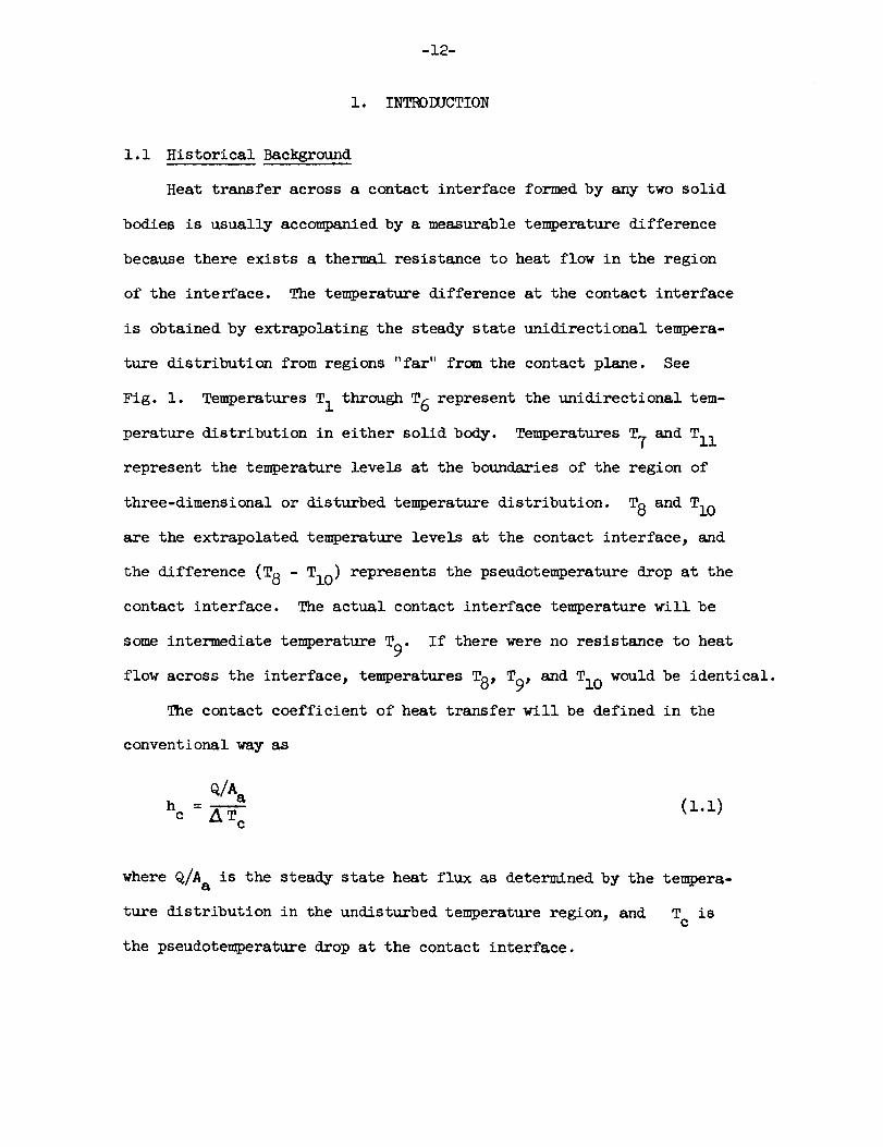
i. i Historical Background
Heat transfer across a contact interface formed by any two solid
bodies is usually accompanied by a measurable temperature difference
because there exists a thermal resistance to heat flow in the region
of the interface. The temperature difference at the contact interface
is obtained by extrapolating the steady state unidirectional tempera-
ture distribution from regions "far" from the contact plane. See
Fig. 1. Temperatures T1 through T6 represent the unidirectional tem-
perature distribution in either solid body. Temperatures T 7 and Tll
represent the temperature levels at the boundaries of the region of
three-dimensional or disturbed temperature distribution. T8 and Tlo
are the extrapolated temperature levels at the contact interface, and
the difference (T8 - Tlo ) represents the pseudotemperature drop at the
contact interface. The actual contact interface temperature will be
some intermediate temperature T9. If there were no resistance to heat
flow across the interface, temperatures T8, T9, and Tlo would be identical.
The contact coefficient of heat transfer will be defined in the
conventional way as
Q/Aahc: A (1.1)
where Q/A a is the steady state heat flux as determined by the tempera-
ture distribution in the undisturbed temperature region, and T isc
the pseudotemperature drop at the contact interface.
-13-
Using the electrical analog the thermal contact resistance is
defined by
R = Z To/Q (1.2)
and can be related to the contact coefficient of heat transfer or con-
ductance as defined by Eq. (i.i) as
1 (1.3)hAc a
It is seen that the thermal contact resistance is the reciprocal of
the contact conductance. Thus, whenever reference is made to the con-
tact conductance, the reciprocal of the thermal contact resistance is
implied. The thermal contact resistance concept will be used through-
out the body of this work since this concept lends itself to nBthemati-
cal analysis.
Over the last two decades and in particular the past ten years,
a large body of literature has been published which deals, with a few
exceptions, primarily with experimental investigations concerning the
thermal resistance between contacting solids. The emphasis on experi-
mental investigations indicates that there was a lack of fundament_l
understanding of the thermal contact phenomenon. The result is that
all the experimental data gathered by the various investigators cannot
be used to predict thermal contact resistance for joints which differ
from those investigated. The experimental data can, however, be used
to show the trends as various parameters are changed. The influence
of these various parameters is shown in Fig. 2. For a more complete
-14°
description of the materials investigated and details of the experi-
mental procedure, this author refers the reader to the very complete
bibliographies of references 9, lO, and ll.
1.2 Review of Parameters Affecting Thermal Contact Resistance
Figure 2 shows the influence on the thermal contact resistance
as the indicated parameters are increased over some range of values.
It is seen that some parameters have a negative influence, i.e., tend
to decrease the thermal resistance while others have a positive influ-
ence. It will be assumed that whenever the influence of one parameter
is considered, all other parameters are constant and, therefore, do
not explicitly affect the discussion.
It should be borne in mind that throughout this discussion we
will be dealing with real or worked engineering surfaces. By this we
mean surfaces which have undergone some engineering process. It is a
well-known fact that all "worked" surfaces exhibit waviness and rough-
ness. These surface characteristics can be determined rather easily
by means of a surface profilometer, and Fig. 6 shows a typical linear
profile of a solid having a wavy, rough surface. An analysis of many
linear profiles indicates that most surfaces have essentially a Gaussian
distribution of asperity heights about some mean plane lying in the
surface, irrespective of the manner in which the surface was prepared,
i.e., milling, grinding, lapping. There is, however, a large differ-
ence in the way the asperities are distributed over the mean plane.
The surface irregularities are the result of the inherent action
of production processes, machine or work deflections, vibrations, and
warping strains. The surface irregularities with the large wavelength
-15-
are termed waviness, the length of these waves depending upon a num-
ber of conditions varying from 0.04 to 0.40 inch. The height can vary
from 80 to 1600 microinches. In general, the longer waves (waviness)
cannot be seen by either eye or microscopic examination. They may,
however, play a controlling part in the behavior of the interface.
In addition to these, most surfaces exhibit finely spaced roughness
that is superimposed on the waviness and is responsible for the finish
of the surface. The finely spaced irregularities are termed roughness
and can range from 2 x lO "6 in. rms for the very smooth surfaces to
about 600 x lO -6 in. rms for the very rough surfaces. Whenever refer-
ence is made to surface asperities, surface roughness is implied. The
curvature of all asperities relative to their height is very large;
i.e., if the asperities are thought to have peaks, the most characteris-
tic range of the included angle at the peak is between 160 ° and 164 °.
The smallest included angle which occurs with the roughest surfaces
would seldom be smaller than 150 °.
It can be seen that when two solid bodies, exhibiting surface
characteristics described above, are brought together under a load,
there will be intimate contact at many small discrete spots, and a
gap will exist in the regions of no real contact. The gap region will
normally be occupied by a fluid, such as air. This brief explanation
will suffice to make clear the discussion on the influence of the vari-
ous parameters on the thermal contact resistance, Fig. 2.
1.2.1 Effect of Apparent Contact Pressure
The first and most obvious parameter to be investigated was the
logd holding the solid bodies together. As the load was increased,
°16-
it was observed that the thermal contact resistance decreased. The
decrease was large initially and becameless as the apparent contact
pressure became quite large. It is expected, from a basic knowledge
of strength of materials, that an increase in apparent contact pressure
would result in a displacement of one surface relative to the other
in the direction of load. This would bring the two surfaces closer
together, thus reducing the size of the gap. A reduction in the size
of the gap means that the surfaces must be in real contact over a
larger region_ i.e., the real area of contact has increased. The rate
of gap decrease and the rate of real area increase should be large
initially when relatively few asperities are in contact, and then the
rate of change should decrease as the number of contacts becomes large.
Also, as the gap size decreases, the thermal resistance through the
fluid in the gap should decrease.
Several attempts were made to correlate the thermal contact resist-
ance against the apparent contact pressure (R o_ pa-m). It was observed
that the exponent varied from practically zero to almost one depending
on several parameters. Even for a fixed system, the exponent would
sometimes be quite different over particular load values. It was noted
that initially m was 1/3 and then increased to one when the load was
quite large. When the contacting surfaces are very smooth but possess
spherical waviness, the contact resistance depends on the load to the
minus 1/S power at moderate contact pressures. This shows that the
physical interaction between the solids is primarily elastic. When
the contacting surfaces exhibit large roughness with essentially no
waviness, the contact resistance varies inversely with the contact
-17-
pressure. This indicates that plastic deformation of the asperities
is important. When the contacting surfaces are very smooth and a fluid
such as air fills the gaps, the contact resistance at high contact
pressures is almost independent of load changes.
A loading-unloading effect has been observed by several inves_±ga-
tors and studied exclusively by Cordier, et al. (13), at the University
of Poitiers. They obtained experimental data for a series of tests
in which the contact pressure was increased stepwise by approximately
300 psi over a range from 0 to 1800 psi; then the contact pressure was
decreased by the same increments until the load wBs again zero. The
measurements were taken at the rate of one every hour. It was noted
that the contact resistance could take on either of two values for any
contact pressure, depending upon whether the measurement is made dur-
ing the loading or unloading cycle.
1.2.2 Effect of Metal Thermal Conductivities
The next obvious parameter to be investigated was the effect of
metal thermal conductivities. It was found that the influence of the
harmonic mean thermal conductivity was practically linear. The reason
that the correlation of thermal resistance with thermal conductivity
is not exactly linear is because the mechanical properties of the solid
bodies cannot be kept constant as the thermal conductivity is changed.
The thermal conductivity effect will not be changed by altering any
of the other parameters.
1.2.3 Effect of Surface Roughness
Considering the influence of surface roughness before the influ-
ence of surface waviness does not imply that roughness effects are
-18-
more pronounced than waviness effects. On the contrary, there are
situations where waviness effects dominate. One should, however,
recognize that the waviness effect can be minimized or reduced com-
pletely by proper preparation of the surface (no waviness present)
or by increasing the load on the contact so that the contact occurs
over the entire apparent area. Roughness, however, cannot be com-
pletely removed by lapping, and its influence on the heat transfer
persists even under the largest contact pressures.
It has been observed that roughness pl_ys an important part in
determining the thermal resistance of a contact interface. The influ-
ence is positive, i.e., increases the resistance. A twofold increase
in roughness can result in a four to fivefold increase in the thermal
resistance. The influence is greatest when the apparent contact pres-
sures are light and the surfaces are relatively smooth, and least when
the contact pressures are high and the surfaces are rougher.
1.2.4 Effect of Surface Waviness
As discussed earlier the influence of surface waviness upon the
thermal contact resistance is dominant under certain conditions of sur-
face geometry and/or apparent contact pressure. It has _been observed
that waviness has a positive influence upon the thermal resistance.
The effect is small for small waviness and becomes very important when
the waviness is large. It has also been noted that a small amount of
surface roughness (which is always present) has a pronounced effect
upon the waviness at light apparent contact pressures. Generally the
presence of some roughness reduces the waviness influence. This sug-
gests that roughness may act as negative influence on the waviness
-19-
because there is an interaction between surface roughness and waviness.
By this we mean that the surface waviness influence upon the thermal
contact resistance cannot be determined without also considering the
effect of surface roughness upon the waviness. Only under limiting
conditions, such as very smooth, very wavy surfaces and very light
apparent pressures, can surface roughness be neglected.
1.2.5 Effect of Interstitial Flui_____dThermal Conductivit_
As observed under Item 1.2.22 there is a negative influence of
interstitial fluid (usually a gas) thermal conductivity. The effect
is linear indicating that the heat transfer is due entirely to conduc-
tion of heat through the fluid layer; i.e., there are no convection
effects in the fluid. A change in the apparent contact pressure, sur-
face characteristics (roughness), and material properties does not
affect the basic influence of fluid conductivity on the thermal resist-
ance.
1.2.6 Effect of Material Hardness
It has been observed that material hardness has a positive influ-
ence upon the thermal contact resistance. By hardness we mean the
pressure at which the material will yield under a compressive load as
determined by any of the standard hardness tests (Brinell, Rockwell,
Knoop, Vickers). There is a good linear correlation between the hard-
ness and the thermal resistance for very rough, very flat (no waviness)
surfaces over a large, apparent contact pressure range.
1.2.7 Effect of Modulus of Elasticit_
A correlation between the thermal contact resistance and Young's
modulus or elastic modulus has been noted. _nere appears to be a
-20-
stronger dependence of the resistance on the elastic modulus as the
surfaces exhibit more waviness and less roughness. In fact, Clausing
and Chao (14) were able to predict the thermal contact resistance for
smooth hemispherical contacts using a contact radius calculated by the
classical Hertzian theory. Their theory failed to predict the resist-
ance for hemispherical contacts which had substantial surface roughness
or when the apparent contact pressure became quite large. The influence
of the elastic modulus is positive; i.e., the thermal resistance increases
with increasing elastic modulus (increasing mechanical resistance). It
is apparent that for certain surface characteristics and load on the
contact, Young's modulus will be important, and the classical elastic
theory may be used to predict the important parameters determing the
thermal contact resistance.
1.2.8 Effect of Mean Contact Temperature Level
It has been observed that there is a correlation between the thermal
contact resistance and the mean contact temperature level. The tempera-
ture influence is negative; i.e., as the temperature level increases,
the thermal resistance decreases. The temperature effect is not very
strong over a large temperature range and only becomes significant when
the temperature level exceeds lO00 OF. The temperature trend is not
unexpected when one considers the various parameters which can influ-
ence the thermal contact resistance and which in turn can be affected
by the temperature level. Both metal and interstitial fluid thermal
conductivities are affected by the temperature level and thus influence
the thermal resistance of the contact. Generally, the metal conduc-
tivity influence is slightly positive while the fluid conductivity
-21-
influence is negative as the temperature level increases. But more
important, the material properties, such as the hardness and the elas-
tic modulus, are influenced by the temperature level. Both effects
are negative; i.e., the hardness and elastic modulus tend to decrease
the thermal contact resistance with increasing temperature level.
This effect is implicitly taken into account when either plastic or
elastic deformation of the surfaces is considered.
For mean contact temperature levels which exceed 1000 OF, radia-
tion heat transfer across the gap becomes significant; i.e., the thermal
contact resistance is determined primarily by the ra_liation resistance.
Since this thermal resistance depends upon the mean temperature to the
1/B power in the linearized form of the radiation equation, it is seen
that the thermal resistance will have a very strong negative dependence
on the temperature level.
Since most engineering problems are concerned with mean contact
temperature levels below lO00 OF, the temperature influence will be
small and will be taken into consideration through the deformation
analysis.
1.2.9 Effect of Interstitial Flui____ddPressure
There is a striking dependence of the thermal contact resistance
upon the interstitial fluid pressure when the fluid is a gas. Consider
the typical thermal resistance-gas pressure relationship shown in Fig. 2i.
The high, horizontal resistance level corresponds to the thermal resist-
ance for surfaces in a hard vacuum, while the low, horizontal resist-
ance level is typical of surfaces at or near atmospheric pressure. The
transition region extends over a very narrow pressure range (about
-22-
lO0 mm Hg) and will be shifted to the left or right depending upon the
surface geometry, the type of gas in the gaps, and the load on the con-
tact. For smoother surfaces the shift is to the left. As the load
on the contact increases, the transition region also shifts to the left.
Also, as the apparent contact pressure increases, the difference between
the two horizontal regions decreases. Generally the higher level (vacuum
region) decreases sharply while the lower level (atmospheric region)
increases slightly. This interesting phenomenon depends upon the rela-
tionship between the mean free path of the gas molecules and the aver-
age or mean gap width. The gap width depends upon the initial surface
geometry, the material properties of the contacting bodies, and the
applied load on the contacting interface.
1.2.10 Effect of Relaxation Time
This phenomenon of relaxation time has been investigated exten-
sively by Cordier. He has observed that the thermal contact resistance
changes with time after initial contact. The influence is negative
and usually takes place over a period of weeks or even months. If
the thermal resistance is plotted against contact time, it is observed
that the resistance decreases continuously and finally assumes a con-
stant level. It is believed that this phenomenon is intimately con-
nected with the hardness of the material and the initial surface geometry.
1.2. ll Effect of Filler Material
By filler material we mean any solid material which is placed
between contacting solid bodies to either reduce or increase the thermal
resistance. It is usually assumed that the filler material is smooth
and uniform in thickness.
-23-
The shaded area in Fig. 2k indicates that there are many ways in
which the filler material can influence the thermal contact resistance.
The variables at one's disposal are the filler thickness, filler thermal
conductivity, and filler hardness or elasticity. It has been observed
that increasing the filler material thickness generally decreases the
thermal resistance (if the original thickness is small _ 1 mil). As
the thickness is increased further, the resistance goes through a mini-
mum value and then begins to increase. Any further increase in filler
material results in yet a higher resistance. The thickness of filler
material at which the thermal resistance is a minimum depends on the
surface geometry, the filler material properties, and the apparent con-
tact pressure. The filler thermal conductivity can have a negative,
zero, or positive influence upon the thermal resistance depending upon
several things such as filler thickness, hardness, and the applied
load. When the filler thickness is large ( _ lO0 mil), the filler
conductivity can have either a negative or positive influence depend-
ing upon the ratio of the solid body/filler thermal conductivity.
When the filler thickness is quite small (_ 1 rail), the filler thermal
conductivity has negligible influence, as the material properties are
more important in determining the effect on the thermal resistance.
It is apparent that a knowledge of the physical interaction between
a filler and the two solid bodies is needed in order to be able to pre-
dict what influence the filler material can have on the thermal con-
tact resistance.
1.2.12 Directional Effect
By directional effect we mean the influence on the thermal contact
resistance which may result from heat flowing from A to B, or from B
to A, where A and B are two dissimilar contacting bodies. It has been
observed by several investigators that there is a significant direc-
tional effect on the thermal resistance whenheat flows between alumi-
numand stainless steel placed in a vacuum. For the sameheat flux
and apparent contact pressure, there may be over lO0 percent differ-
ence in the thermal contact resistance for heat flowing from aluminum
to stainless steel than from stainless steel to aluminum. The magni-
tude of this difference is seen to depend upon the surface geometry
(roughness, waviness), the material properties, the apparent contact
pressure, and the level of heat flux.
It is believed that this phenomenon is the result of local thermal
strains due to the relative temperature gradients between the actual
contact spots and surrounding material. Due to local thermal strains,
the number and size of contacts will be influenced differently as the
heat flows from A to B or from B to A. This may result in significant
changes in the thermal contact resistance. In order to predict this
phenomenon, it is necessary to have knowledge of the interaction of
solid bodies under various heating conditions. This includes knowing
the effect of surface roughness and waviness, as well as the material
properties.
1.3 Summary of Parameters Influencing Thermal Contact Resistance
The brief review of the many parameters which have some influence
on the thermal contact resistance clearly shows that this contact phe-
nomenon is quite complex. One would be rather naive to think that any
one theory could predict the thermal resistance over all possible ranges
of the many parameters considered to be important. Each area of interest
-25-
will require special consideration in order to evaluate the relative
importance of one parameter over another, e.g., influence of inter-
stitial fluid relative to the influence of the contact spots.
One underlying theme runs through all of the discussions. It
becomes very clear that the interaction of solid bodies under loading
conditions is of paramount importance. The influence of interstitial
fluid, filler material, the radiation effect, and the directional effect
will depend upon the gap and, therefore, upon the surface geometry and
the interaction of the solid bodies.
The factors which determine the real contact area between contigu-
ous solids can be divided into two areas of importance: surface geome-
try (roughness, wBviness) and surface interaction (plasticity, elasticity,
hardness). It is obvious that during the development of contact, both
areas are mutually interrelated, and it is impossible to determine some
of them without a knowledge of others. For example, the size of the
actual contact area, which depends upon the geometrical properties of
the contacting surfaces, determines the actual pressure acting on the
asperities, while the roughness determines the asperity density over
the contacting area. The present knowledge of surface interactions
does not permit one to use either the classical elasticity or plasticity
theory unless the compressed surfaces are of regular geometrical form
_ith either perfectly elastic properties or for the case of plasticity
without roughness.
The contact process for real surfaces cannot be reduced to purely
elastic or to purely plastic deformation of the microscopic asperities.
Contact interactions of two solids are generally of an elastoplastic
-26-
or elastoviscous nature. This is due to the fact that the initial con-
tact usually occurs between the highest asperities which are few in
number and which must bear all the applied load. There is subsequent
redistribution of the pressure to the other asperities after the first
contacting asperities have been crushed, and the total applied load
is finally supported by the entire surface layer of the bodies. The
possibility is not excluded that the macroscopic surface deviations
(waviness) can change during the loading. Also, there may be a perma-
nent change in the characteristics of the roughness during the com-
pression.
It is evident (and bears repeating) that the shape, height, and
distribution of the macroscopic (wBviness) and microscopic (roughness)
surface irregularities are some of the most important'factors deter-
mining the real contact area under loading conditions.
The most important physical (mechanical) properties are the modu-
lus of elasticity, the hardness or yield pressure of the asperities,
and the plasticity in the determination of the following: l) real
contact pressure; 2) the displacement or approach of the surfaces as
a result of the deformation of the surfaces under compression; and
3) the actual area of contact (number and size of contact spots).
-27-
2. THERMAL CONTACT RESISTANCE
2.1 Introduction
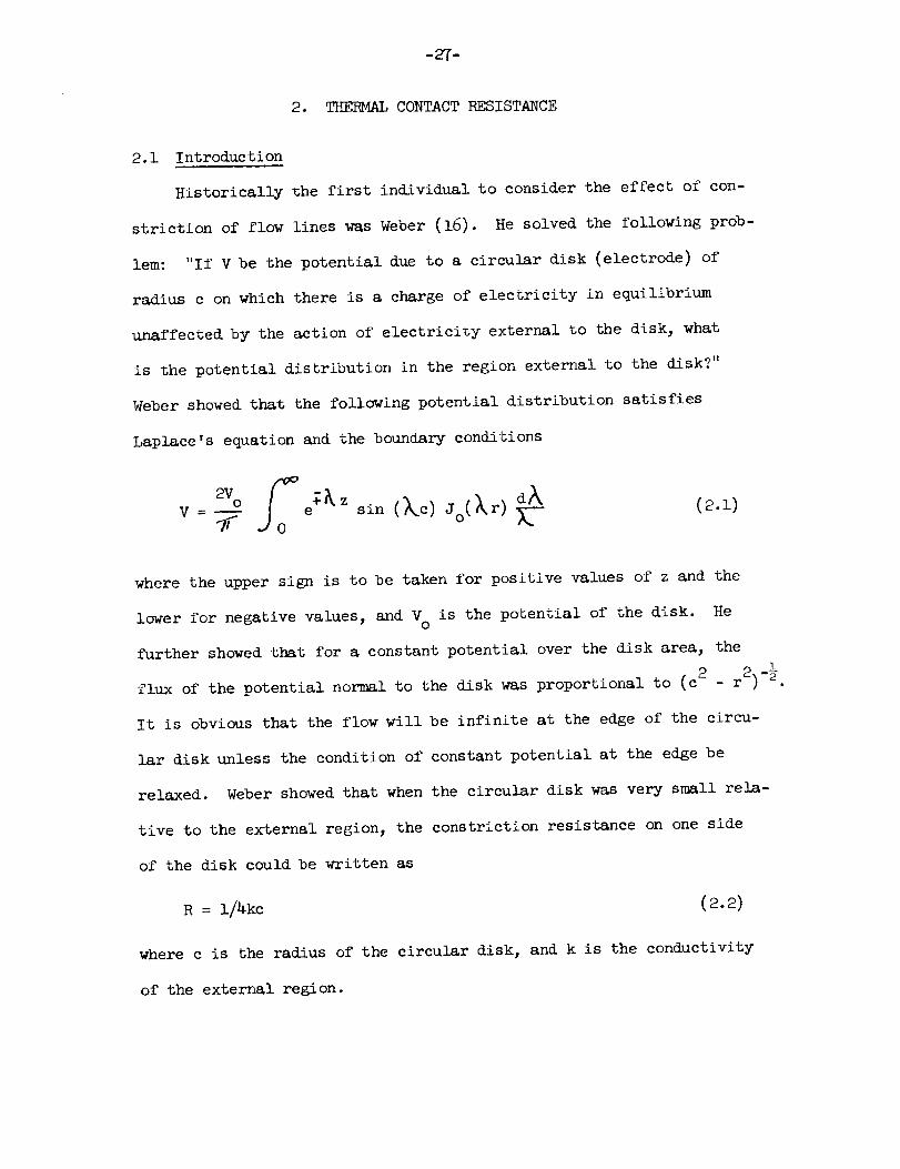
Historically the first individual to consider the effect of con-
striction of flow lines was Weber (16). He solved the following prob-
lem: "If V be the potential due to a circular disk (electrode) of
radius c on which there is a charge of electricity in equilibrium
unaffected by the action of electricity external to the disk, what
is the potential distribution in the region external to the disk?"
Weber showed that the following potential distribution satisfies
Laplace's equation and the boundary conditions
2V° e sin (kc) Jo(kr) _-- (2.1)v= 7
where the upper sign is to be taken for positive values of z and the
lower for negative values, and V° is the potential of the disk. He
further showed that for a constant potential over the disk area, the
flux of the potential normal to the disk was proportional to (c2 - r2) -½.
It is obvious that the flow will be infinite at the edge of the circu-
lar disk unless the condition of constant potential at the edge be
relaxed. Weber showed that when the circular disk was very small rela-
tive to the external region, the constriction resistance on one side
of the disk could be written as
R = I/4kc (2.2)
where c is the radius of the circular disk, and k is the conductivity
of the external region.
-28-
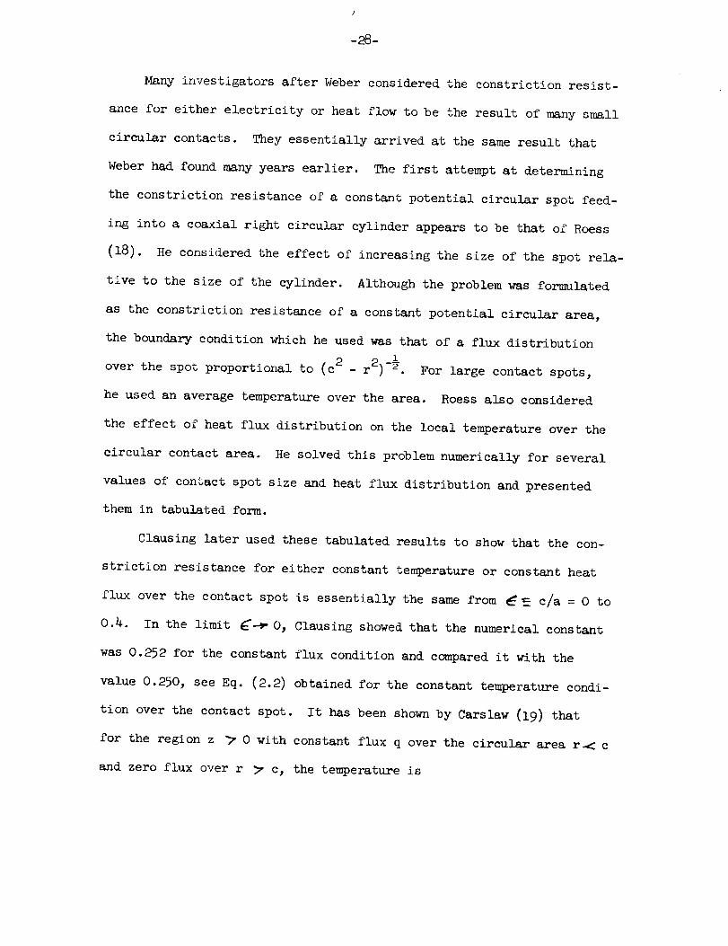
Many investigators after Weber considered the constriction resist-
ance for either electricity or heat flow to be the result of many small
circular contacts. They essentially arrived at the same result that
Weber had found many years earlier. The first attempt at determining
the constriction resistance of a constant potential circular spot feed-
ing into a coaxial right circular cylinder appears to be that of Roess
(18). He considered the effect of increasing the size of the spot rela-
tive to the size of the cylinder. Although the problem was formulated
as the constriction resistance of a constant potential circular area,
the boundary condition which he used w_s that of a flux distribution
over the spot proportional to (c 2 - r2) -½. For large contact spots,
he used an average temperature over the area. Roess also considered
the effect of heat flux distribution on the local temperature over the
circular contact area. He solved this problem numerically for several
values of contact spot size and heat flux distribution and presented
them in tabulated form.
Clausing later used these tabulated results to show that the con-
striction resistance for either constant temperature or constant heat
flux over the contact spot is essentially the same from E_ c/a = 0 to
0.4. In the limit _-_0, Clausing showed that the numerical constant
was 0.252 for the constant flux condition and compared it with the
value 0.250, see Eq. (2.2) obtained for the constant temperature condi-
tion over the contact spot. It has been shown by Carslaw (19) that
for the region z _ 0 with constant flux q over the circular area r< c
and zero flux over r _ c, the temperature is
_0 _
T= qc e-_ zk
-29-
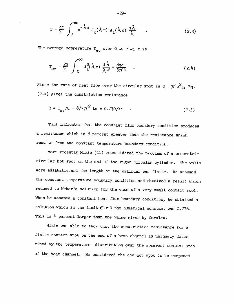
jo(_r) jl(kC) d_ (2.3)
The average temperature Tav over O_ r< c is
Since the rate of heat flow over the circular spot is Q =_c2q, Eq.
(2.4) gives the constriction resistance
R = Tav/Q = 8/3_ "2 kc = 0.270/kc (2.5)
This indicates that the constant flux boundary condition produces
a resistance which is 8 percent greater than the resistance which
results from the constant temperature boundary condition.
More recently Mikic (ll) reconsidered the problem of a concentric
circular hot spot on the end of the right circular cylinder. The walls
were adiabatic, and the length of the cylinder was finite. He assumed
the constant temperature boundary condition and obtained a result which
reduced to Weber's solution for the case of a very small contact spot.
When he assumed a constant heat flux boundary condition, he obtained a
solution which in the limit _-_0 the numerical constant was 0.276.
This is 4 percent larger than the value given by Carslaw.
Mikic was able to show that the constriction resistance for a
finite contact spot on the end of a heat channel is uniquely deter-
mined by the temperature distribution over the apparent contact area
of the heat channel. He considered the contact spot to be composed
-30-
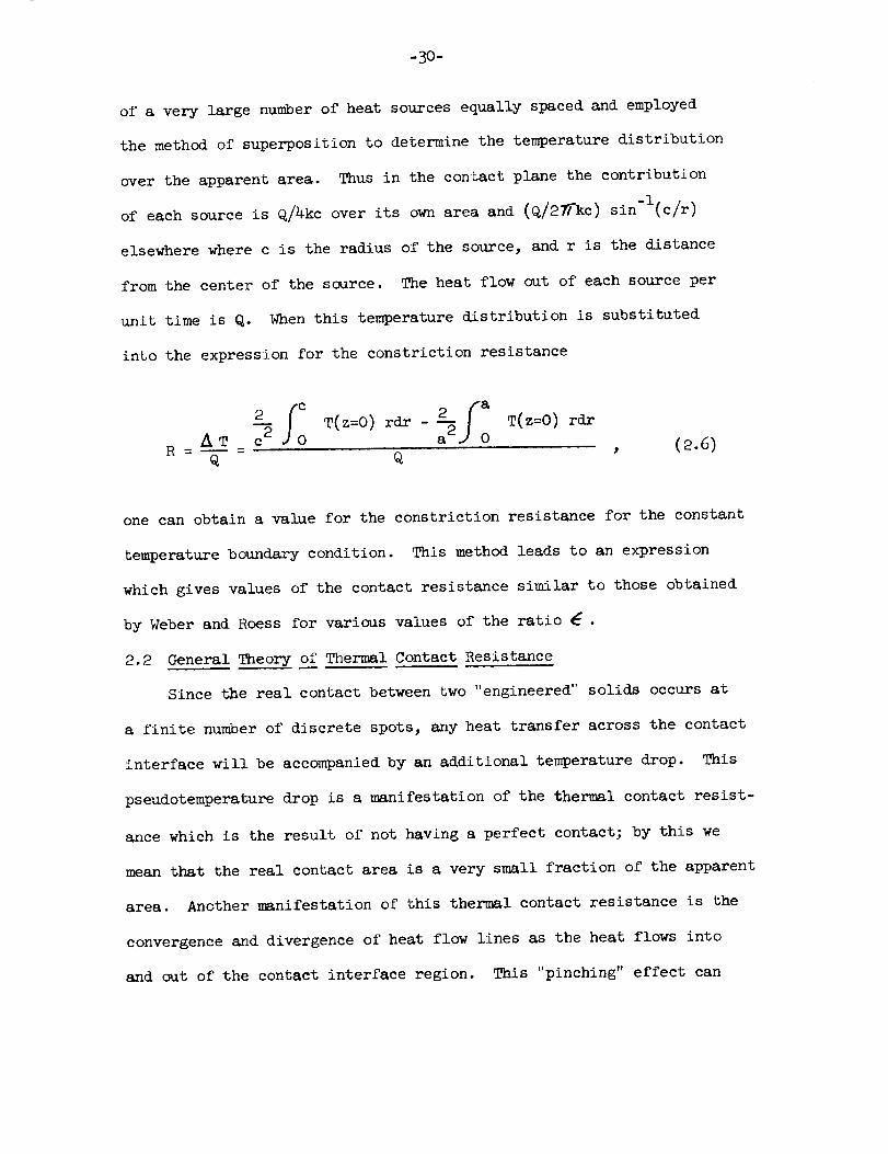
of a very large numberof heat sources equally spaced and employed
the method of superposition to determine the temperature distribution
over the apparent area. Thus in the contact plane the contribution
of each source is Q/4kc over its ownarea and (Q/2_kc) sin-l(c/r)
elsewhere where c is the radius of the source, and r is the distance
from the center of the source. The heat flow out of each source per
unit time is Q. Whenthis temperature distribution is substituted
into the expression for the constriction resistance
_ fc 2 f_ T(z=O) rdrT(z=O) rdr - -_AT c 0 a (2.6)
R= Q Q
one can obtain a value for the constriction resistance for the constant
temperature boundary condition. This method leads to an expression
which gives values of the contact resistance similar to those obtained
by Weber and Roess for various values of the ratio _ •
2.2 General Theory_of Thermal Contact Resistance
Since the real contact between two "engineered" solids occurs at
a finite number of discrete spots, any heat transfer across the contact
interface will be accompanied by an additional temperature drop. This
pseudotemperature drop is a manifestation of the thermal contact resist-
ance which is the result of not having a perfect contact; by this we
mean that the real contact area is a very small fraction of the apparent
area. Another manifestation of this thermal contact resistance is the
convergence and divergence of heat flow lines as the heat flows into
and out of the contact interface region. This "pinching" effect can
-31-
be visualized more easily if we restrict our discussion to contiguous
surfaces in a hard vacuum environment and also assume that radiation
heat transfer across the gaps is negligible; i.e., the radiation
thermal resistance is extremely large relative to the "pinching"
effect. All the heat crossing the contact interface can flow only
through the real contact area. The pinching effect is maximum when
the contact spots are few in number and small in size. It will be
shown later in this discussion that the number, size, and distribu-
tion of contact spots are more important than the magnitude of the
total real area in reducing the thermal contact resistance.
The presence of a fluid in the gaps or radiation effects tends
to alleviate the "pinching" effect and thus reduce the thermal con-
tact resistance. The presence of a very thin, very soft metal foil
also tends to alleviate the "pinching" effect by increasing the density
of contacts over the value without the presence of the foil.
With this "pinching" effect in mind, let us examine closely the
physical interaction of two nominally flat, rough surfaces (no wavi-
ness present). Since there is no waviness, the small contact spots
will appear randomly over the entire apparent area. This picture w-ill
not be true if the contiguous surfaces have a definite lay, and they
are mated either parallel or perpendicular to this lay. We shall
restrict ourselves to a random distribution of contact spots over the
apparent area. The diameter of these contact spots will vary over
some range from the smallest diameter (probably determined from sur-
face energy conditions) to some maximum diameter (which cannot be
determined at this moment). It is expected that the largest diameter
-32-
can be (and often is) an order of magnitude larger than the smallest.
The frequency of occurrence of the smallest can be orders of magni-
tude larger than the occurrence of the largest diameter, so that ulti-
mately the total real area due to the smallest contact spots is practi-
cally equal to the real area of the largest. But most important, the
bulk of the real contact area is due to the manycontact spots having
somemeancontact diameter which is approximately the average of the
smallest and largest diameter.
It has been observed that the meancontact spot diameter is practi-
cally independent of the apparent contact pressure. This does not mean
that the sizes of the contact spots do not change. The smallest diame-
ter may change slightly, and it is expected that the largest size will
change significantly as the load on the contact interface is increased.
With every increase in apparent pressure, there is an increase in the
total number of contacts. The result is that the bulk of the total
real area is still due to those contacts having a diameter intermedi-
ate to the smallest and largest diameter. This new meandiameter
corresponding to the new larger apparent pressure is practically
unchanged.
It mast be realized that a rough surface consists of manyvery
small peaks and valleys, which are randomly distributed about somemean
plane lying in the surface. It has been shownthat the contained angle
at the peaks is seldom smaller than 150° and is usually about 162°.
The value of 150° corresponds to the_roughest surface which one may
encounter. This meansthat the peaks are more like very long rolling
plains than high mountains. Whentwo such peaks or asperities come
-33-
into contact, it resembles the contact between two very large hemi-
spheres touching over a small (relative to the radii of curvature of
the asperities) circular spot.
Since we are examining the case of heat transfer only through the
contacts (hard vacuum, negligible radiation effect), the heat transfer
model which suggests itself for the case of few and smll contacts is
that of a contact spot on a semi-infinite body. As the apparent con-
tact pressure increases, the number of contacts increases greatly, and
the heat transfer model must be changed. Here we can assume that each
contact spot is fed by a heat channel having adiabatic walls; i.e.,
all the heat passing some plane contained by the heat channel and which
is far from the contact zone must pass through the contact spot. The
mthematic solution to this model should go into the solution for the
first model in the limit as the diameter of the contact spot becomes
verymuch smaller than the heat channel diameter.
Throughout this discussion we have referred to contact spot diame-
ter implying that the contacts are circular. We expect the contact-
ing asperities (which need not be hemispherical) will seldom touch
along an axis passing through their centers of curvature. They will
touch on their shoulders thus producing elliptical contact spots. We
believe that these will differ only slightly from circular spots, and,
therefore, to facilitate the mathematics we assume circular contact
spots throughout the discussion.
It will further be assumed that the contact interface (it is rea-
sonable to assume that the interface can be slightly curved, due to a
very hard curved solid contacting a flat soft solid) lies in a surface
-34-
which if the contact were perfect would be an isothermal surface.
This assumption is important to the argument presented in Appendix A.
Here it is shown that the contact spots are all at a uniform tempera-
ture (this will yield a particular solution for the thermal contact
resistance of an elemental heat channel). It is further shown that
all contact spots, irrespective of size, shape, or distribution over
the apparent contact area, have the same uniform temperature. This
is true only for the restrictions stated above.
2.3 Thermal Contact Resistance for an Elemental Heat Channel
The following discussion will follow closely the work done by
Mikic (ll), who determined the thermal contact resistance for an ele-
mental heat channel. He assumed that all the contact spots have the
same circular area and also that the contact spots are uniformly dis-
tributed over the contact interface. This picture of the contact spot
size and distribution is not strictly valid and will be discussed later.
For contacts in a vacuum and because the contacting asperities usually
have a very small slope, Mikic assumed the elemental heat channel to
consist of a circular hot spot on the end of a right circular cylinder.
For negligible radiation heat transfer, the area beyond the contact
spot can be considered to be adiabatic. The sides of the heat channel
by definition will also be adiabatic. The radius of the heat channel
will be calculated by means of the contact spot density as defined by
the constant radius, uniformly distributed contact spot model. One
half of the elemental heat channel is shown in Fig. 9 with the boundary
conditions which must be satisfied by the solution to Laplace's
-35-
differential equation over the entire region defined by the elemental
heat channel.
The two cases which he solved differed only in the boundary condi-
tions prescribed over the contact spot. The first case considered a
uniform temperature over the contact spot (this requires that the heat
1/2 2flux over the contact spot be hemispherical, i.e., q = Q/27Tc - r
where c is the contact spot radius). In the second case it was assumed
that the heat flux over the contact spot was uniform. These two boundary
conditions will determine the minimum and maximum thermal resistances
which can be developed due to the contact spot. Any other temperature
or heat flux distribution over the contact spot will produce a thermal
resistance whose magnitude will lie between the limiting values. It
is for this reason that the two cases were studied in great detail.
The complete details can be found in reference (ll).
0nly the salient features of the theory will be presented here
in order to show which geometric parameters are needed. It has been
shown that the thermal contact resistance for one half an elemental
heat channel can be expressed as
frkE
where k is the thermal conductivity of the heat channel material,
is the average contact spot radius, and _(_/a) is the dimensionless
factor which depends upon the boundary condition over the contact spot
and the ratio of the spot radius to the heat channel radius.
For the case of uniform contact spot temperature or hemispherical
heat flux over the contact spot, _ can be expressed as
-36-
c c_i(_) i a _in(O<n a E) Jl(O<na g)
n=l (O_a)3 O.2(O<n_)o
(2.8)
with Jl(O<'na ) = 0 . (2.9)
For the case of uniform heat flux over the contact spot, _ can
be expressed as
oo
n=l
m
n E
(2.lO)
As in Eq. (2.8) the roots are determined by Jl(C_na ) = 0.
An examination of Eqs. (2.8) and (2.10) shows that _2 exceeds _i
over the entire range of the ratio _/a. The maximum difference is
just slightly less than lO percent; i.e., the thermal contact resist-
ance for the constant heat flux boundary exceeds the constant tempera-
ture boundary condition by about lO percent.
Since all physical phenomena appear to follow the path of least
resistance, it would not be premature to assume that the constant tem-
perature boundary condition is the appropriate one. This boundary
condition, however, requires a hemispherical heat flux distribution
which has a singularity at the very edge of the boundary, i.e., r = _.
It might be more reasonable to assume that the constant temperature
condition is valid over the major portion of the real contact and that
in the vicinity of the edge, another condition is valid, say a constant
flux. We shall, however, assume throughout the discussion that the
-37-
constant temperature condition prevails over the entire real contact
area.
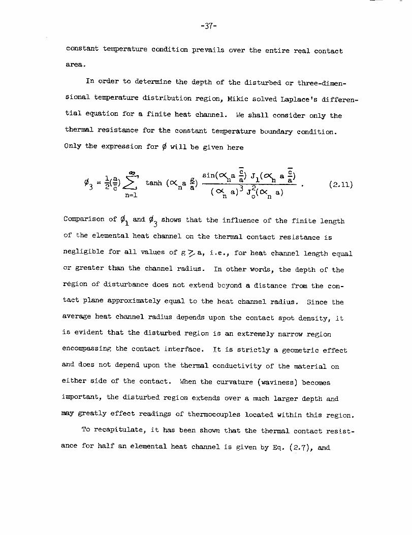
In order to determine the depth of the disturbed or three-dimen-
sional temperature distribution region, Mikic solved l_place's differen-
tial equation for a finite heat channel. We shall consider only the
thermal resistance for the constant temperature boundary condition.
Only the expression for _ will be given here
n=l
sin(O_a _) Jl(O_ a _) (2.11)
(O<na (% a)3Jo2(O<na) "
Comparison of _i and _3 shows that the influence of the finite length
of the elemental heat channel on the thermal contact resistance is
negligible for all values of g _ a, i.e., for heat channel length equal
or greater than the channel radius. In other words, the depth of the
region of disturbance does not extend beyond a distance from the con-
tact plane approximately equal to the heat channel radius. Since the
average heat channel radius depends upon the contact spot density, it
is evident that the disturbed region is an extremely narrow region
encompassing the contact interface. It is strictly a geometric effect
and does not depend upon the thermal conductivity of the material on
either side of the contact. When the curvature (waviness) becomes
important, the disturbed region extends over a much larger depth and
may greatly effect readings of thermocouples located within this region.
To recapitulate, it has been shown that the thermal contact resist-
ance for half an elemental heat channel is given by Eq. (2.7), and
-38-
the geometric factor _ is given by Eq. (2.8) for the constant tempera-
ture boundary condition. The analysis was based on steady-state condi-
tions, hard vacuum, negligible radiation, and the absence of an oxide
film. The model is based on the physical contact between typical hemi-
spherical asperities assuming that the circular contact spot is much
smaller than the radii of curvature of the contacting asperities.
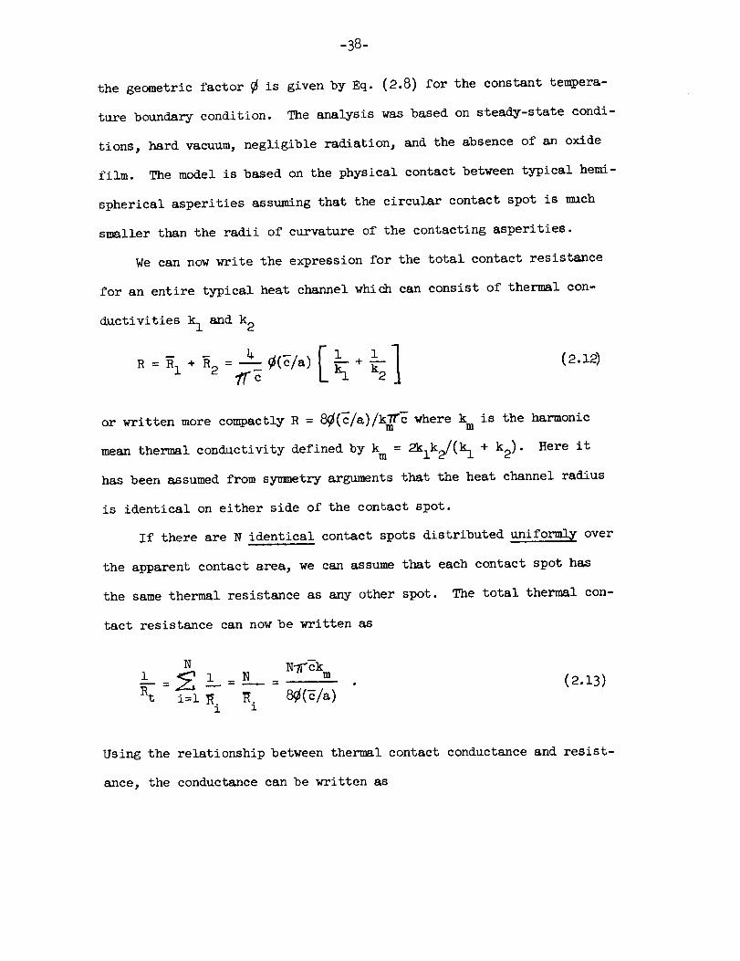
We can now write the expression for the total contact resistance
for an entire typical heat channel which can consist of thermal con-
ductivities kI and k 2
R = R1 + R2 = 4._¢(_/a) +?"re
or written more compactly R = where k is the harmonic
mean thermal conductivity defined by k = 2klk2/(k I + k2). Here it
has been assumed from sy_netry arguments that the heat channel radius
is identical on either side of the contact spot.
If there are N identical contact spots distributed uniformly over
the apparent contact area, we can assume that each contact spot has
the same thermal resistance as any other spot. The total thermal con-
tact resistance can now be written as
N NV_k
1 _l__N m1 1
(2.13)
Using the relationship between thermal contact conductance and resist-
ance, the conductance can be written as
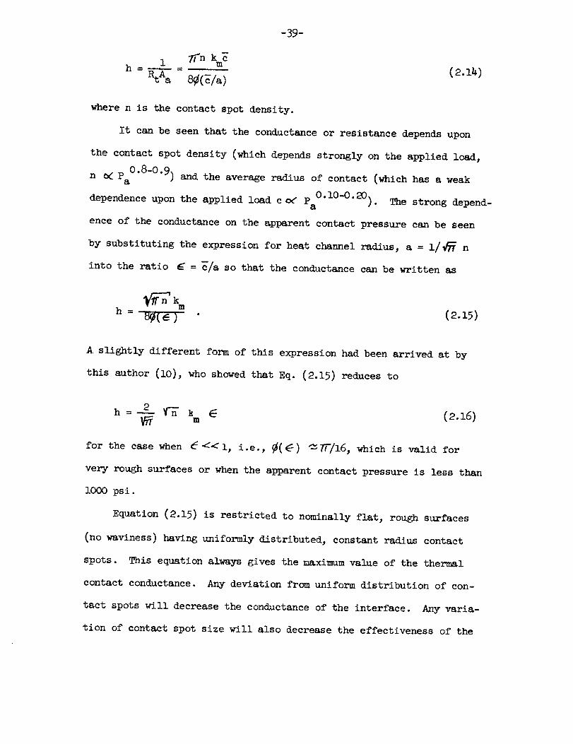
-39-
(2.14)
where n is the contact spot density.
It can be seen that the conductance or resistance depends upon
the contact spot density (which depends strongly on the applied load,
n _Pa 0"8-0"9) and the average radius of contact (which has a weak
0.10-0.20) The strong depend-dependence upon the applied load cog Pa
ence of the conductance on the apparent contact pressure can be seen
by substituting the expression for heat channel r_dius, a = i/_ n
into the ratio 6 = _/a so that the conductance can be written as
h
m
" (2.15)
A slightly different form of this expression had been arrived at by
this author (lO), who showed that Eq. (2.15) reduces to
2 V-_ _ 6 (2.16)h=-_- m
for the case when _I, i.e., _(_) _77-/16, which is valid for
very rough surfaces or when the apparent contact pressure is less than
lO00 psi.
Equation (2.15) is restricted to nominally flat, rough surfaces
(no w_viness) having uniformly distributed, constant radius contact
spots. This equation always gives the maximum value of the thermal
contact conductance. Any deviation from uniform distribution of con-
tact spots will decrease the conductance of the interface. Any varia-
tion of contact spot size will also decrease the effectiveness of the
-4o-
contacts thus reducing the conductance of the interface. The devia-
tion from uniform distribution of constant size contact spots becomes
more evident with decreasing surface roughness and/or increasing con-
tact pressure. These effects on the overall thermal contact resist-
ance will be examined in great detail in the following chapter.
When the contiguous surfaces exhibit large curvature (waviness)
as well as roughness, the contact spots are confined to a portion of
the apparent area, which is called the contour area. The contour area
is the projected area determined by the outer limits of the microcon-
tacts. In the region beyond the contour area, there is no physical
contact between the touching surfaces. The contour area lying wholly
within the apparent area can occupy a fraction or the entire portion
of the apparent area depending upon the surface characteristics, the
mterial properties, and the load on the interface. The effect of
surface waviness will be discussed in some detail later.
-41-
3. THE EFFECTS OF CONTACT SPOT SIZE AND MALDISTRIBUTION
3.1 Contact Between Nominally Flat, Rough Surfaces
Worked metallic surfaces, whether turned, ground, or sandblasted,
exhibit a random distribution of asperity heights about some mean plane
lying in the surface ( 9 ). The distribution of the asperities over
the apparent area, in general, will not be random, but will exhibit
a lay. The lay or predominant direction of the asperities will depend
upon the process (turning, grinding, blasting). A turning process
will produce a circular pattern, while a grinding process will produce
a linear pattern.
Unless two identical surfaces are matched exactly, it is expected
that even those surfaces having a lay will produce microcontaets which
are randomly distributed over the apparent area. Since the contacting
surfaces are nominally flat, the microcontacts will be found anywhere
in the total region defined by the total apparent area.
Let us consider the interaction of two nominally flat, rough sur-
faces, bearing in mind the facts just presented. Initially the con-
tact will occur at the few highest asperities. As the load increases,
these initial contact spots increase in size, and newer and smaller
contacts just begin to form. Upon increasing the load still further,
the first contacts grow even larger, the second group of contacts also
increases in size, and still newer and smaller contacts appear. The
process is repeated with each increase of the pressure on the contact
interface.
One can see from this description that as nominally flat, rough
surfaces come into contact under a load, there will be real contact
-42-
over a large number of discrete microcontacts which differ in size,
density, and probably shape.
Autoradiographical data (8), Figure 8, show that the microcon-
tacts are almost circular and that they vary in size and frequency
of occurrence. The largest microcontacts are sparce, while the smaller
ones are many. This is further substantiated by the friction and wear
work of Rabinowicz (22) who measured the size distribution of wear
particles formed during the relative slip of one metallic solid over
another under a contact pressure. He also demonstrated that the size
of wear particles formed is directly related to the size of microcon-
tacts present. It was also observed that the size of the largest parti-
cle can be an order of magnitude larger than the smallest particle size.
In the following discussion it _ili be assumed that the microcon-
tacts are circular in shape. This is done because circular shapes
are amenable to mathematical analysis, and it is unlikely that the
actual shapes differ much from elliptical shapes having major and
minor axes approximately equal. Based on these outstanding facts,
it is necessary for us to re-examine the existing thermal contact
resistance theory to determine whether the contact size distribution
is significant.
3.2 Elemental Heat Flux Tube
We define an elemental heat flux tube as a volume which encom-
passes a contact spot and extends some distance into either solid
forming the contact. The surface which bounds the heat flux tube is
called the control surface; it is always a closed suri_ce. The sur-
faces through which the heat enters and leaves the heat flux tube will
-43-
be isothermal surfaces while the remaining surface will always be adia-
batic. One isothermal surface will be in one solid while the other
isothermal surface will be in the second solid. The axis of the heat
flux tube will be parallel to the axis of the contact spot. Every ele-
mental heat flux tube can be separated, in the surface of contact, into
two parts because the heat flow pattern on either side of the contact
is similar, and the surface of contact, as well as the contact spot, is
isothermal. The bounda_# conditions over the surface of contact can
be used to determine the contact or constriction resistance. The total
resistance of the elemental heat flux tube will be the sum of the
resistances of the two parts considered separately. It will be shown
shortly that the linear dimension of the contact spot determines the
size of the heat flux tube and, therefore, the quantity of heat flow-
ing through the surface of contact. In the absence of an interstitial
fluid and negligible radiation heat transfer across the gaps, all the
heat entering the heat flux tube must pass through the contact spot.
The larger contact spots will conduct more heat than the smaller con-
tacts, Figure i0.
We shall consider in this work that the elemental heat flux tube
is a right circular cylinder. The ends of the cylinder are the iso-
thermal surfaces (planes) while the sides which are parallel to the
axis of the cylinder are adiabatic. Other shapes of heat flux tubes
can arise which are but modifications of the one which we shall use.
As examples, consider the contact between concentric pipes or concen-
tric spheres, Figure ii.
-44-
There are two possible types of heat flux tubes: one in which
the contact spot is placed right in the center of the contact plane
or one in which the contact spot is not equidistant to the boundary
of the contact plane. We define the symmetric heat flux tube or sym-
metric contact as the one in which the axis of the contact spot is
coincident with the axis of the heat flux tube. There is symmetry
in any plane perpendicular to the contact plane. As stated earlier
this problem was first considered by Weber (16) who obtained the con-
striction resistance for a small circular isothermal spot. Later
several other investigators considered the effect of the relative
size of the contact spot. They showed that when the contact spot
was large, the resistance was not only a function of the linear dimen-
sion of the contact, but also a function of the relative size of the
contact. Thus a contact spot whose radius is 1 percent of the heat
flux tube radius would offer 26.5 times more resistance than a contact
spot whose radius is 20 percent of the heat flux tube radius. This
is 32 percent greater because of the relative size effect, Figure 12.
We now define an asymmetric heat flux tube as one in which the
axis of the contact spot is not coincident with the axis of the heat
flux tube. There is a finite distance between the axes, and there is
sy_netry in only one plane--the perpendicular plane which is co-planar
with the two axes. The temperature distribution will be different in
every other perpendicular plane. The contact plane, as well as the
contact spot, will remain isothermal even when the asymmetry is a
maxirf_Im.
-45-
Intuitively one feels that the asymmetric contact should not be
able to conduct as much heat as the symmetric contact, especially when
the contact spot is in the vicinity of the boundary of the heat flux
tube. Also a relatively large contact spot should be more sensitive
to small displacements from its symmetric position, while a very small
contact spot would be relatively insensitive to a similar displacement.
A series of liquid analog tests were conducted to determine the
effect of asymmetry for a typical heat flux tube. An analysis was
made to correlate the experimental data with the relative displacement
and the relative size of the contact spot, Appendix B. The experimental
data showed that the relatively large contact spots are quite sensi-
tive to small displacements, while the relatively small contact spots
were less influenced by the asymmetry. It was observed that the asym-
metric effect was a maximum when the contact spot displacement was a
maximum and that this effect was a constant _, independent of the
relative size of the contact spot, Figure 13.
There are two ways of viewing the asymmetric effect when the con-
tact spot is relatively small. One way is to fix the boundary; then
the asym_netric effect can be represented by an area over which the
contact could be moved to have only a nominal increase in the resist-
ance, Figure 18. The second way is to fix the contact spot in space
and allow the boundary to alter its shape about the usual circular
boundary, Figure 19. In short, the constriction resistance of a very
small contact spot is independent of the shape of the boundary of the
heat flux tube as long as the minimum or maximum distance from the
contact spot to the boundary is not less than (b -_ ) or greater
-46-
than (b + J) where b is the linear dimension of the plane of contact,
and _ is the displacement corresponding to a nominal increase in the
resistance.
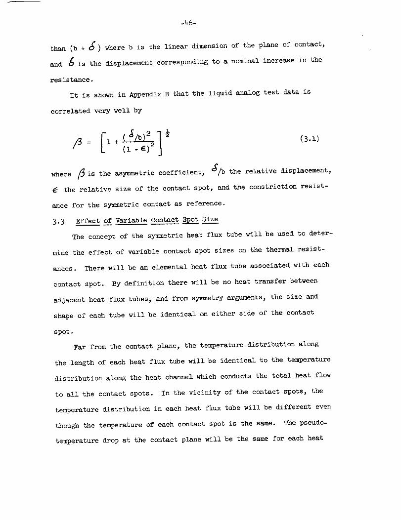
It is shown in Appendix B that the liquid analog test data is
correlated very well by
l
_ --- _i ÷ ( _/b)_ 1_(i - g=)_ (3.1)
where _ is the asymmetric coefficient, J/b the relative displacement,
the relative size of the contact spot, and the constriction resist-
ance for the symmetric contact as reference.
3.3 Effect of Variable Contact Spot Siz____e
The concept of the symmetric heat flux tube will be used to deter-
mine the effect of variable contact spot sizes on the thermal resist-
ances. There will be an elemental heat flux tube associated with each
contact spot. By definition there will be no heat transfer between
adjacent heat flux tubes, and from sy_netry arguments, the size and
shape of each tube will be identical on either side of the contact
spot.
Far from the contact plane, the temperature distribution along
the length of each heat flux tube will be identical to the temperature
distribution along the heat channel which conducts the total heat flow
to all the contact spots. In the vicinity of the contact spots, the
temperature distribution in each heat flux tube will be different even
though the temperature of each contact spot is the same. The pseudo-
temperature drop at the contact plane will be the same for each heat
-47-
flux tube.
immediately write
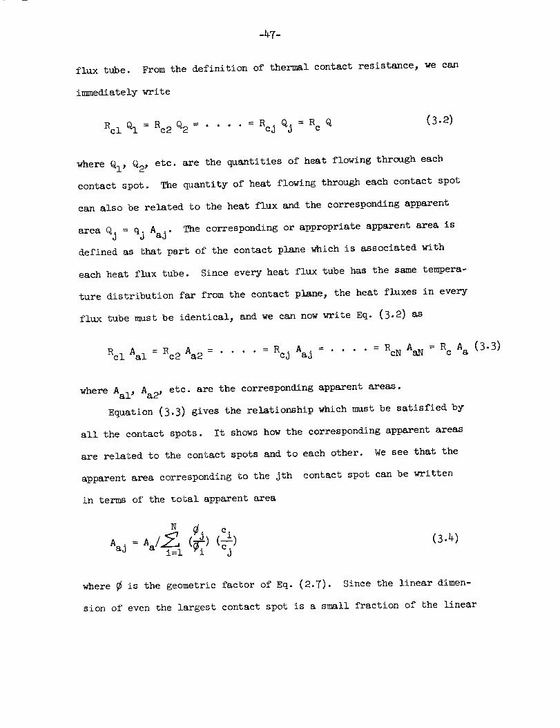
From the definition of thermal contact resistance, we can
Rcl Q1 = Rc2 Q2 ..... = Rej QJ = Rc Q(3.2)
where Ql' Q2' etc. are the quantities of heat flowing through each
contact spot. The quantity of heat flowing through each contact spot
can also be related to the heat flux and the corresponding apparent
The corresponding or appropriate apparent area isarea Qj = qj Aaj.
defined as that part of the contact plane which is associated with
each heat flux tube. Since every heat flux tube has the same tempera-
ture distribution far from the contact plane, the heat fluxes in every
flux tube must be identical, and we can now write Eq. (3.2) as
Rc I Aa I = Rc 2 Aa 2 ..... = Rc j Aa j ..... = RcN AaN = Rc Aa (3.3)
where Aal, Aa2, etc. are the corresponding apparent areas.
Equation (3.3) gives the relationship which must be satisfied by
all the contact spots. It shows how the corresponding apparent areas
are related to the contact spots and to each other. We see that the
apparent area corresponding to the jth contact spot can be written
in terms of the total apparent area
N °iAaj: Aa/ ( )i=l " j
(3.4)
where _ is the geometric factor of Eq. (2.7). Since the linear dimen-
sion of even the largest contact spot is a small fraction of the linear
-48-
dimension of the corresponding apparent area, _j/_i _ 1.0 for any
two contact spots. This means that the size of any corresponding
apparent area is determined by the linear dimensions of the corres-
ponding contact spot and the entire set of contact spots. The total
apparent area is subdivided among the contact spots according to the
relation given in Eq. (3.4).
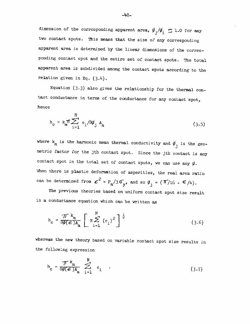
Equation (3.3) also gives the relationship for the thermal con-
tact conductance in terms of the conductance for any contact spot,
hence
N
hc : ci/ jAa (3.5)i=l
where km is the harmonic mean thermal conductivity and _j is the geo-
metric factor for the jth contact spot. Since the jth contact is any
contact spot in the total set of contact spots, we can use any _.
When there is plastic deformation of asperities, the real area ratio
can be determined from E2 = pa/3%, and so _j = (-_/16 - E/4).
The previous theories based on unifo_n contact spot size result
in a conductance equation which can be written as
h = m N_
c 8¢(_)A a i=l (3.6)
whereas the new theory based on variable contact spot size results in
the following expression
c 8¢(_)A a i:l _ (3.7)
-49-
Liquid analog tests clearly demonstrate that for the same number of
contact spots and the same total real area, Eq. (3.6) will over pre-
dict the conductance by as much as 34 percent while Eq. (3.7) agrees
extremely well with the tests. As the variation in contact spot size
becomes smaller, both Eqs. (3.6) and (3.7) predict conductances which
agree with test data, and in the limit when all contacts are the same
size, Eq. (3.6) reduces to Eq. (3.7).
3.4 Effect of Maldistribution of Contact Spot__ss
We have shown that a certain fraction of the total apparent area
corresponds to each contact spot. This function is determined by the
linear dimension of the contact spot relative to the sum of the linear
dimensions of all the contact spots. The position of the jth corres-
ponding apparent area is determined by every contact spot. Not only
the neighboring contact spots but also the most distant contact spots
contribute towards determining where the jth corresponding apparent
area will be located. If the jth contact spot falls on the center of
the jth corresponding apparent area, it forms a symmetric contact, and
it is properly distributed. Should the jth contact spot not fall on
the center of the jth corresponding apparent area, it forms an asym-
metric contact, and it is not properly distributed but maldistributed.
The maldistribution will be determined by the relative displacement
between the axes of the contact spot and the corresponding heat flux
tube.
The constriction resistance for a maldistributed contact spot is
now given by
-50-
(3.7)Rcj cj .
Suppose that all the other contact spots are properly distributed,
then only the jth contact spot is maldistributed. The temperature
distribution far from the contact plane is the same in the jth asym-
metric heat flux tube as in any other heat flux tube. This means
that the flux through the jth corresponding apparent area is the same
as any other corresponding apparent area; i.e., (Qj/Aaj) = (Q1/Aal)"
_epseudotemperature drop at the contact plane must be the same for
every heat flux tube including the jth tube, therefore,
Aal c 3 (3.8)
AaJ : cI /3j
where Cj $ ¢I" The contribution of the jth contact spot has been
reduced due to its maldistribution. Every contact spot which is mal-
distributed can be treated in a similar fashion. If every contact of
the total set of contact spots shows some maldistribution but there
is no preferred direction, the conductance can now be written as
N
hc: i:l(3.9)
It is seen that the maldistribution correction appears as a reduction
in the linear dimension of the contact spot; i.e., the effective radius
of the contact spot is smaller than the actual radius by the factor_ •
_¢nen the maldistribution is such that all the contact spots are dis-
placed in a particular pattern, then an additional correction will
-51-
have to be made. This can occur with a wBvy surface where the contact
spots are crowded together towards the center of the apparent area.
This situation cannot be handled directly by the maldistribution fac-
tor _.
A series of liquid analog tests were conducted to check the validity
of Eq. (3.9)- In one series the numberand size of the contact spots
were fixed, but their position in the contact plane was varied. It is
seen that a positive or negative displacement in the radial direction
results in an increase in the contact resistance. For the tests con-
ducted the maldistribution varied from 9 to 18 percent, and the theory
agreed reasonably well with the test data. As stated above the theory
would not predict the effect of displacing all the contact spots to
the boundary or to the center of the apparent area.
3.5 Contact Resistance Between Rough, Wavy Surfaces
It was noted earlier that the contact spots are confined to a
particular region of the apparent area if the contacting surfaces have
large curvature (wmviness). For hemispherical waviness, the contact
spots will appear in a circular region which is defined as the contour
area. The contour area is determined by the outer limits of the con-
tact spots, Figure 16. By definition there is no physical contact
beyond the contour area. In the absence of an interstitial fluidand
negligible radiation heat transfer across the gaps, the heat flow across
the interface will be confined to the contour region in the vicinity of
the contact plane. The total resistance _ is postulated to consist of
the waviness resistance (constriction of the heat flow lines to the con-
tour area) and the roughness resistance (pinching of the heat flow lines
-52-
due to the contact spots). Weassumethat these two effects can be
linearly added to obtain the overall thermal contact resistance.
It has been proved that the contact spots are all at a uniform
and commontemperature independent of their size, shape, and distribu-
tion. The only restrictions are that they be in a plane which would
be an isothermal plane if the contact were perfect. If there is no
waviness, the contour area is identical with the apparent area, and
the contact spots by definition will be found over the entire contact
plane. An isothermal plane (1) will exist at some distance gl from
the contact plane (0). This distance is quite small being proportional
to the radius of the elemental heat flux tube (the contact spot radius
is much smaller than the heat flux tube radius; i.e., E_< 1). If the
contact were perfect, planes (0) and (1) would be coincident, and there
would be no thermal contact resistance.
Consider now the situation where the contact spots completely fill
the contour area, but the conto_mr area is smaller than the apparent area.
Planes (0) and (1) are coincident and isothermal. Another isothermal
plane (2) will exist at some distance g2 from the contact plane (0).
'Fnis distance is large, being proportional to the radius of the heat
channel if the contour area is very small. In the limit as the contour
area becomes as large as the apparent area, plane (2) is coincident with
the contact plane and, therefore, coincident with planes (0) and (1).
Thus for perfect contact, all three isothermal planes are coincident
(gl = 0 and g2 = 0), and there is no contact resistance.
'When both roughness and waviness are present, we hypothesize that
all three isothermal planes exist and that the effect of roughness can
-53-
be determined by considering the thermal contact resistance between
planes (0) and (1), while the effect of waviness can be determined by
considering the thermal contact resistance between planes (1) and
(2). The total contact resistance will be the sum of the two resist-
ances.
We also assume that the distances gl and g2 are linearly propor-
tional to the difference between the radius of the heat channel (or
flux tube) and the contour radius (or contact spot radius). It is
obvious that as the contour area approaches the size of the apparent
area, g2 decreases, becoming zero in the limit, and, therefore, the
waviness resistance is zero.
Since the contact spot is always much smaller than the heat flux
tube area, gl_ O, and it is approximately equal to the heat flux tube
radius. Only in the limit of very smooth surfaces (mirror finish) does
gl _ O. We conclude that the effect of surface roughness is always
present, but that its overall effect will be dependent upon the magni-
tude of the waviness resistance. For lightly loaded, very wavy "smooth"
surfaces, the waviness resistance will be dominant, and the roughness
resistance will be negligible. The surface roughness may, however, have
a significant effect upon the size of the contour area. _en the con-
tacting surfaces are very rough with slight " t "ou -of-flatness, and
heavily loaded, the roughness resistance will be dominant while the
waviness resistance is negligible. The surface waviness may be quite
important in determining the pressure distribution over the contact
plane and thus indirectly affects the roughness resistance.
-54-
We can now state that for rough, wavy contacting surfaces in a
vacuum and negligible radiation heat transfer, the overall thermal
contact resistance is
R
1 2
°i ii=l
(3.1o)
where the first term represents the thermal resistance due to the con-
tact spots, and the second term represents the thermal resistance due
to the contour area. We have shown that because of the wBvlness influ-
ence, the resistance of the contact spots will have to be corrected for
size variation as well as maldistrlbution. The geometric factor for
the contact spots can be approximated by _l = (q_/16 - _/4). The
thermal resistance Of the contour area is inversely proportional to the
contour radius. This radius will depend upon the geometry of the con-
tacting surfaces, the material properties, and the applied load. Unless
the surfaces are quite smooth and quite wavy, the contour radius will
generally be a large fraction of the apparent radius. The contour geome-
tric factor _2 can be obtained from Figure 12.
An equation similar to Eq. (3.10) has been proposed by Holm (21)
and Kragel'ski (29) for the total contact resistance of rough spheres
1 1 (3.11)R = 2Nks c 2ksC
where c is the radius of a contact spot, and C is the contour radius.
This equation is restricted to a contact which consists of many very
-55-
small contact spots (all the samesize) properly distributed in a very
small contour area. A contact which satisfies these conditions is quite
uncommon and would occur only if the contacting surfaces were quite rough
and quite _Bvy, and the contact load were very light. It can be seen
that Eq. (3.10) will reduce to Eq. (3.11) when all these restrictive
conditions are met. Eq. (3.10) is therefore a more general expression
for the overall thermal contact resistance for a rough, wavy contact.
Multiple contour regions will occur whenever periodic waviness is
present. Equation (3.10) should then be changed to take this into con-
sideration. For small out-of-flatness, the contour areas will be almost
as large as the corresponding apparent areas, and the maldistribution
correction will have to be applied to the contour resistance. It has
been shown that the asymmetry effect is most important when the contour
area is large relative to the apparent area. We believe that the con-
tour asy_netry effect will not directly affect the roughness resistance.
Since the contour asymmetry effect becomes important for large contour
areas when the roughness resistance is usually dominant, the overall
resistance may be little influenced by maldistribution of contour areas.
-56-
4. SURFACE DEFOHMATION
4. i Introduction
Real surfaces exhibit roughness and wBviness. As a consequence
of the roughness, the real contact between two solids always occurs
at discrete spots which are finite in number and very small. As a
consequence of the waviness, the discrete contact spots are generally
confined to a particular region of the apparent area called the con-
tour area. The extent of the contour area will depend upon the sur-
face waviness, roughness, material properties, and the applied load.
At the points of real contact, generally at the highest parts of con-
tacting asperities, the local pressure is extremely large, resulting
in plastic yielding of the softer material (if a soft and hard material
are in contact). The stress over the contour area will usually be
very much less than the local stresses, so that the formation of the
contour area can be considered as an elastic process. The application
of a greater load decreases the distance and separation between the
surfaces, thereby increasing the number of discrete contact spots and
also increasing the contour area. The contacting asperities themselves,
however, may either be deformed plastically, with some workhardening
taking place, or elastically. Elastic deformation occurs only in those
asperities, usually those coming into contact last, in which the local
stresses are relatively low. They generally occur at the boundary of
the contour area where the stress distribution over the contour area
approaches a zero value.
Since the shape and size of the asperities depend upon the mechani-
cal process used to generate the surface, the number, shape, and size
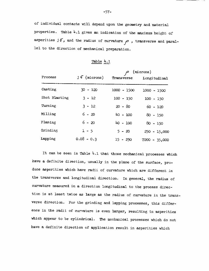
-57-
of individual contacts will depend upon the geometry and material
properties. Table 4.1 gives an indication of the maximum height of
asperities j _-, and the radius of curvature p , transverse and paral-
lel to the direction of mechanical preparation.
Table 4.1
Process j_ (microns)
(microns)
Trans verse Longitudinal
Casting 30 - 120 i000 - 1500 I000 - 1500
Shot Blasting 3 - 12 I00 - 150 i00 - 150
Turning 3 - 12 20 - 80 60 - 120
Milling 6 - 20 40 - i00 80 - 150
Planing 6 - 20 40 - lO0 80 - 150
Grinding 1 - 5 5 - 20 250 - 15,000
Lapping 0.08 - 0.3 15 - 250 7000 - 35,000
It can be seen in Table 4.1 that those mechanical processes which
have a definite direction, usually in the plane of the surface, pro-
duce asperities which have radii of curvature which are different in
the transverse and longitudinal direction. In general, the radius of
curvature measured in a direction longitudinal to the process direc-
tion is at least twice as large as the radius of curvature in the trans-
verse direction. For the grinding and lapping processes, this differ-
ence in the radii of curvature is even larger, resulting in asperities
which appear to be cylindrical. The mechanical processes which do not
have a definite direction of application result in asperities which
-58-
have radii of curvature which are the same in mutually perpendicular
directions. These asperities can be considered to have a hemispheri-
cal shape. Since the surfaces used in this study have been prepared
by glass blasting, it will be assumed that we always have hemispheri-
cal asperities coming into contact.
The waviness of surfaces encountered in practice is the result
of many mechanical and thermal factors and is, therefore, quite varia-
ble. When the surface waves are smooth and have regular shapes, such
as semicylinders or hemispheres, the contour area can be calculated
from the classical Hertz theory. If the waviness is not regular, then
the contour area must be determined empirically. In this work it will
be assumed that the waves are hemispherical, so that when two such
waves contact, the resulting contour area will be circular.
_.2 Elastic Deformation of a Smooth Hemispherical Surface
In this section we shall review the basic theory of the elastic
deformation of smooth hemispherical surfaces. The results of this
analysis will be used to determine the deformation of a rough, hemispheri-
cal surface. Let two smooth solid hemispheres be in contact at a point
0 as shown in Figure 22. The surfaces have a common tangent pBane at
O, which we take as the xy-plane. Take the positive Z-direction as
being in either solid and denote the corresponding coordinates as Z 1
and Z 2. Near a point of ordinary contact with the xy-plane, the equa-
tion of the surfaces can be written with sufficient accuracy as
2 f z2 rR/2f (4.1)zI = r /2 1 ' = 2
where/1 and /2 are the radii of curvature of the two solids.
-59-
Let us assume that the two solids are now pressed together by an
applied force and approach each other by a short distance 0(. A deforma-
tion occurs near the original point of contact, and the two solids will
be in contact over a small but finite portion of their surfaces. Let
_l and_r2 be the components (along the Z 1 and Z 2 axes, respectively)
of the corresponding displacements for points on the surfaces of the
two solids. The broken lines in Figure 22 show the surfaces as they
would be in the absence of any deformation, while the solid lines show
the surfaces of the deformed bodies. It is seen from the figure that
the equation
(z I + _I) + (z 2 +_2) =
holds everywhere in the region of contact.
of contact, we have
Zl + _J-1 + z2 +_2 7 o<
(4.2)
At points outside the region
(4.3)
The local displacement can be related to the approach of the solids
and the equation of the surfaces as
f.,O"l+_Y2= o<-- F- + = --_ .(4.4)
We denote by Pz(X, Y) the pressure between the two deformed solids at
points in the region of contact; outside this region, Pz = O. To
determine the relation between Pz and the local displacements_ 1 and
6j-2, we can with sufficient accuracy regard the surfaces as plane
and use the results of point loading on the half space.
-60-
A. E. H. Love (23) has shownthat Boussinesq's solution for a
point load can be extended to the case of a distributed load of
intensity Pz(_, _ ) acting on the bound_ of the half space, where
}, _ are the coordinates of a point in the loaded region of the
boundary.
Summingup the effects of such forces, we obtain the displace-
ments in the elastic half space due to the given distributed load.
1- l P (I'7)(4.5a)
2 = _fT_ 2 r d
where _-and E are the Poisson ratio and the elastic modulus, respec-
tively, of the two solids, and r = {(x- I )2+ (y _ 2)2 _. Since
Pz = 0 outside the region of contact, the integration extends only
over the loaded region. It should be noted that from these formulae,
the ratio 6_-1/_ 2 is constant, independent of loading,
1 - q-2 2l) (z - g2)
(4.6)
and are identical for the same materials.
The relations (4.2) and (4.6) together give the displacements
6J_l and_ 2 at every point of the contact region, while relations
(4.5a, b) and (4.6) relate to points outside the contact region.
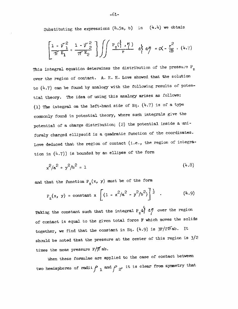
-61-
Substituting the expressions (4.5a, b) in (4.4) we obtain
Ii i 2 IE1 _E 2 r
(4.7}
This integral equation determines the distribution of the pressure Pz
over the region of contact. A. E. H. Love showed that the solution
to (4.7) can be found by analogy with the following results of poten-
tial theory. The idea of using this analogy arises as follows:
(1) The integral on the left-hand side of Eq. (4.7) is of a type
co_nonly found in potential theory, where such integrals give the
potential of a charge distribution; (2) the potential inside a uni-
formly charged ellipsoid is a quadratic function of the coordinates.
Love deduced that the region of contact (i.e., the region of integra-
tion in (4.7)) is bounded by an ellipse of the form
x2/a2+ y2/b2 = 1(_..8)
and that the function Pz(X, Y) must be of the form
pz(X, y) = constant x (1 - x2/a 2 - Y
Taking the constant such that the integral Pzd_ d_ over the region
of contact is equal to the given total force F which moves the solids
together, we find that the constant in Eq. (4.9) is 3F/27_ab. It
should be noted that the pressure at the center of this region is 3/2
times the mean pressure F_ab.
When these formulae are applied to the case of contact between
it is clear from sy_netry thattwo hemispheres of radii f 1 and f 2'
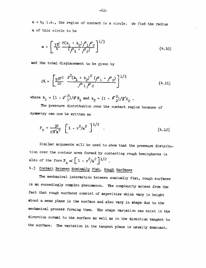
-62-
a = b; i.e., the region of contact is a circle. Wefind the radius
a of this circle to be
.{. + (4.1o)
and the total displacement to be given by
[gz__ F2(5 + _2)2 (f I + F 2)] 1/3o<= Pip2 (4.n)
wherek1 = (1 - 1]-_)/_ _'l andk2 : (1 - 6_)/_. 2 .
The pressure distribution over the contact region because of
symmetry can now be written as
Pz 2,_a2 (_.12)
Similar arguments will be used to show that the pressure distribu-
tion over the contour area formed by contacting rough hemispheres is
also of the fo1_ Pz _ I1 - r2/a 2]1/2
4.3 Contact Between Nominally Flat, Rough Surfaces
The mechanical interaction between nominally flat, rough surfaces
is an exceedingly complex phenomenon. The complexity arises from the
fact that rough surfaces consist of asperities which vary in height
about a mean plane in the surface and also vary in shape due to the
mechanical process forming them. The shape variation can exist in the
direction normal to the surface as well as in the direction tangent to
the surface. The variation in the tangent plane is usually dominant.
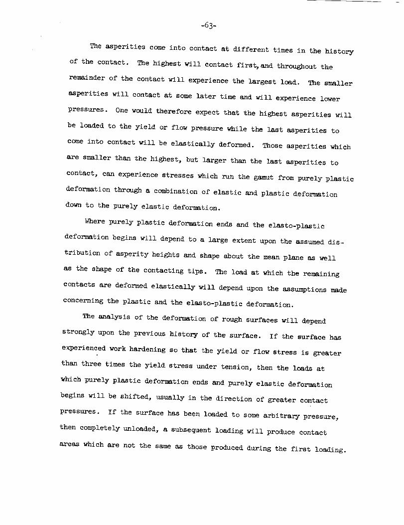
i63-
The asperities come into contact at different times in the history
of the contact. The highest will contact first, and throughout the
remainder of the contact will experience the largest load. The smaller
asperities will contact at some later time and will experience lower
pressures. One would therefore expect that the highest asperities will
be loaded to the yield or flow pressure while the last asperities to
come into contact will be elastically deformed. Those asperities which
are smaller than the highest, but larger than the last asperities to
contact, can experience stresses which run the gamut from purely plastic
deformation through a combination of elastic and plastic deformation
down to the purely elastic deformation.
Where purely plastic deformation ends and the elasto-plastic
deformation begins will depend to a large extent upon the assumed dis-
tribution of asperity heights and shape about the mean plane as well
as the shape of the contacting tips. The load at which the remaining
contacts are deformed elastically will depend upon the assumptions made
concerning the plastic and the elasto-plastic deformation.
The analysis of the deformation of rough surfaces will depend
strongly upon the previous history of the surface. If the surface has
experienced work hardening so that the yield or flow stress is greater
than three times the yield stress under tension, then the loads at
which purely plastic deformation ends and purely elastic deformation
begins will be shifted, usually in the direction of greater contact
pressures. If the surface has been loaded to some arbitrary pressure,
then completely unloaded, a subsequent loading will produce contact
areas which are not the same as those produced during the first loading.
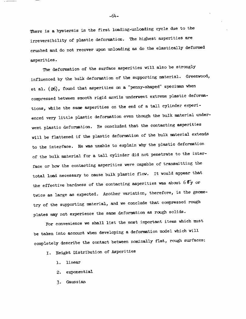
-64-
There is a hystersis in the first loading-unloading cycle due to the
irreversibility of plastic deformation. The highest asperities are
crushed and do not recover upon unloading as do the elastically deformed
asperities.
The deformation of the surface asperities will also be strongly
influenced by the bulk deformation of the supporting material. Greenwood,
et al. (26), found that asperities on a "penny-shaped" speciman when
compressed between smooth rigid anvils underwent extreme plastic deforma-
tions, while the same asperities on the end of a tall cylinder experi-
enced very little plastic deformation even though the bulk material under-
went plastic deformation. He concluded that the contacting asperities
will be flattened if the plastic deformation of the bulk material extends
to the interface. He was unable to explain why the plastic deformation
of the bulk material for a tall cylinder did not penetrate to the inter-
face or how the contacting asperities were capable of transmitting the
total load necessary to cause bulk plastic flow. It would appear that
the effective hardness of the contacting asperities was about 6 _-y or
twice as large as expected. Another variation, therefore, is the geome-
try of the supporting material, and we conclude that compressed rough
plates may not experience the same deformation as rough solids.
For convenience we shall list the most important items which must
be taken into account when developing a deformation model which will
completely describe the contact between nominally flat, rough surfaces:
I. Height Distribution of Asperities
i. linear
2. exponential
3. Gaussian
-65-
II. Shape of Asperity Tips
i. cones
2. spheroids
3. ellipsoids
III. Material Deformation
I. plastic
2. elastic
3 • elasto-plastic
IV. Deformation History
i. initi_l lo_ding
2. subsequent loading
3- work hardening
V. Bulk Geometry
1. very thin plates
2. thick plates
We might add under the heading "Shape of Asperity Tips" that we must
make some assumption concerning the distribution of the radii of curva-
ture of the contacting asperities, usually assumed to be constant.
Most worked surfaces have a Gaussian distribution of asperity
heights. Some surfaces, e.g., bead-blasted ones, are Gaussian while
some are not. Over a limited range the Gaussian distribution approxi-
mates to an exponential distribution. This occurs in the highest
asperity range where the distribution may be exponential. Thus a
Gaussian distribution is a good approximation even for the exponential
distribution. Of course, the distribution will be neither Gaussian or
exponential if the asperities have experienced plastic deformation
-66°
during some previous contact. Most deformation theories have been based
on a Gaussian distribution of asperity heights about some mean plane.
The assumption that the contacting asperities are spheroids has
been used by almost all the investigators. It was further assumed that
the force between the contacting asperities Ms transmitted along a line
passing through the centers of the spheroids. This assumption precludes
any contact _hich might occur on the shoulders of the asperities. For
bead-blasted surfaces these assumptions are probably quite good in pre-
dicting the physical interaction between nominally flat 3 rough surfaces
over a large load range. For surfaces prepared in some other _nner,
new assumptions will have to be made.
If plastic deformation of the contacting asperities is assumed,
then only the yield pressure of the softer material (if a soft and hard
material are in contact) is required to predict the total real area of
contact. No infor_Btion about the height distribution nor the shape of
the asperity tips is required for purelyplastic deformation. On the
other hand, the plastic deformation theory will not yield any informa-
tion regarding the number or sizes of the contact spots which make up
the total real area. In conjunction with the plastic deformation theory,
we need some information about the topography of the contacting surfaces
and how the topography chauges with relative approach of the contacting
surfaces. Only in this way can information be obtained about the num-
ber and size of the individual contact spots.
If one assumes elastic deformation of the contacting asperities,
then both height distribution and asperity shape are necessary to pre-
dict the contact size, the number of contacts, and the relative approach
-6T-
of the contacting surfaces. These three parameters can be related to
the radii of curvature of the contacting asperities and the compliance
of the contacting surfaces. Greenwood and Williamson (26) used this
approach to determine the criterion for the onset of plastic deformation
of the asperities. They were able to show that the contact behavior of
a surface can be described in terms of two material properties: the
hardness or flow pressure at the asperity tips and the elastic modulus;
and two topographic parameters: the radii of curvature of the contact-
ing asperities and the spread of asperity heights. They have called
this parameter the plasticity index. The plasticity index merely deter-
mines the load at which the asperity deformation changes from purely
elastic to plastic. They concluded that actually the plasticity index
completely dominates the behavior, and the load has little effect. _._en
the plasticity index is less than 0.6 (very smooth surfaces), plastic
contact could be caused only if the surfaces were forced together under
very large nominal pressures. _en the index exceeds 1.O (most worked
surfaces fall in this category), plastic flow of contacting asperities
will occur at even the lowest nominal pressures.
Mikic (ll) also concluded that during initial contact over 95 per-
cent of the total real area results from plastic deformation of the con-
tacting asperities while 5 percent of real area is due to elastic deforma-
tion. His analysis was based on arguments similar to the ones used by
Greenwood.
No theory to date has taken into consideration the effects of subse-
quent loadings or work hardening. It is well known that when the load
on a contact is reduced to some lower level, the real area of contact
-68-
is larger than the value which would correspond to the same load on
the first loading cycle. This agrees with the assumption that there
is plastic deformation of asperities during the initial loading. After
several loading-unloading cycles, the contact between the surfaces
becomes completely elastic. The topography has been altered due to
the plastic deformation, and the distribution of the highest asperities
is no longer exponential or Gaussian. The radii of curvature have
become very large, almost infinite for those asperities which have
been completely flattened.
Work hardening is always present to a small or large degree depend-
ing upon the material and the method of preparation. It is not clearly
understood how important work hardening is or when it becomes important
in the loading/deformation cycle.
No surface deformation theory has included the effect of bulk
geometry, i.e., the effect of the support material upon the deformation
of the contacting asperities. As stated earlier, it has been observed
experimentally that asperities which rest on a very thick layer of
material can support very large loads before plastic deformation occurs.
On the other hand, asperities which rest on a very thin layer of material
will undergo complete plastic deformation.
It can be seen that the mechanical interaction between nominally
flat, rough surfaces is quite complex, and no theory has been developed
which can predict the number and size of individual contact spots under
any load condition. We shall, therefore, restrict our attention to
bead-blasted surfaces (Gaussian distribution, spheroidal asperity tips),
undergoing initial loading (predominantly plastic deformation). The
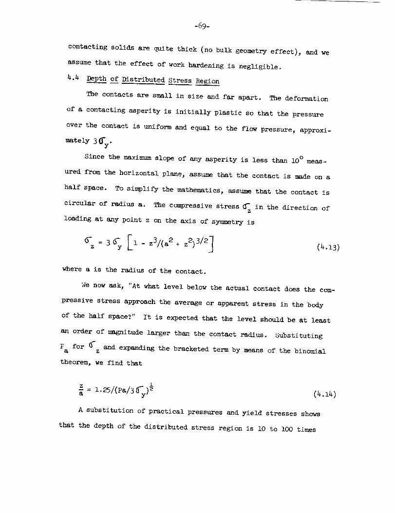
-69-
contacting solids are quite thick (no bulk geometry effect), and we
assume that the effect of work hardening is negligible.
4.4 Depth of Distributed Stress Region
The contacts are small in size and far apart. The deformation
of a contacting asperity is initially plastic so that the pressure
over the contact is uniform and equal to the flow pressure, approxi-
mately 3 _y.
Since the maximum slope of any asperity is less than lO ° meas-
ured from the horizontal plane, assume that the contact is made on a
half space. To simplify the mathematics, assume that the contact is
circular of radius a. The compressive stress _z in the direction of
loading at any point z on the axis of symmetry is
+ (4.13)
where a is the radius of the contact.
We now ask, "At what level below the actual contact does the com-
pressive stress approach the average or apparent stress in the body
of the half space?" It is expected that the level should be at least
an order of magnitude larger than the contact radius. Substituting
P for _ and expanding the bracketed term by means of the binomialZ
theorem, we find that
z = 1.25/(P /3a (4.14)
A substitution of practical pressures and yield stresses shows
that the depth of the distributed stress region is lO to lOO times
-70-
the radius of the contact. Wecan arrive at a more interesting expres-
sion which relates the depth to the radius of the corresponding appar-
ent area by means of Pa/3(_y
z/b= 1.25
= _ 2 a2/b 2P
(4.15)
It is obvious that the distributed stress region is very thin.
For most engineering surfaces the maximum depth will range from about
lO0 mils for very light loading down to about lO mils for large con-
tact pressures. When the thickness of the distributed stress region
is compared with the radius of curvature of the waviness component of
the surface finish, it is seen that the ratio is m_ch less than unity.
We can now consider the deformation of a rough,_avy surface to con-
sist of two parts; the plastic or elasto-plastic deformation of the
contacting asperities (which is a local phenomenon), and the elastic
deformation of the surface lying beyond the distributed stress region.
4.5 Local Displacements Du___eto Plastic Deformation of Asperities
_Wnenever a region of the half space is loaded, there occur local
displacements in the direction of loading. The surface of the half space
at some distance from the axis of loading will also experience displace-
ments in the vertical direction, Figure 24. We ask, "At what distance
from the axis of symmetry does this effect become negligible?"
We again consider the case of a uniform load (due to plastic
deformations of contacting asperities) distributed over the area of
a circle of radius a and consider the displacement, in the direction
of loading, of a point P on the surface of the half space at a distance
r from the center of the circle. By superposition of point loads, the
total displacement at P is given by (24)
-71-
(' 4 ='1= /rE _ -r
(4.16)
where _-and E are the material properties, q is the pressure on the
circle, and E' and K' are the complete elliptic integrals with modulus
k= a/r
K ! ___2 dx andE' = xdx
-
_'-l- k 2 sin 2 x
To obtain the displacement at the boundary of the loaded circle,
we take r = a in Eq. (4.16) and find
(r = a) 4(1 - v-I)qa (4.17)= ' ]_E
A more interesting and useful expression can be obtained by tak-
ing the ratio of the displacements at point P and at the boundary
2 1_(r) r [E' -(i- 2)K' (4o18)_(r = a) = K _ r
This expression is independent of the material properties and the
magnitude of the uniform stress over the circle. The _isplacement at
any point P depends upon the radius of the loaded circle. Equation (4.18)
could be rewritten, replacing the term r/a by (r_)(b/a) and letting
r_b. The expression would then give the ratio of the displacement
at r = b to the displacement at the boundary of the loaded circle.
The displacement ratio then becomes a function of the ratio of the
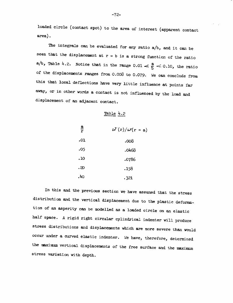
-72-
loaded circle (contact spot) to the area of interest (apparent contact
8_rea ).
The integrals can be evaluated for any ratio a/b, and it can be
seen that the displacement at r = b is a strong function of the ratio
aa/b, Table 4.2• Notice that in the range 0.O1-< _ _ O.10, the ratio
of the displacements ranges from 0.008 to 0.079. We can conclude from
this that local deflections have very little influence at points far
away, or in other words a contact is not influenced by the load and
displacement of an adjacent contact.
Table 4.2
a
_-(r)/ar(r = a)
.01 .008
•O5 .O468
.i0 •0786
._o .158
• 4o .32l
In this and the previous section we have assumed that the stress
distribution and the vertical displacement due to the plastic deforma-
tion of an asperity can be modelled as a loaded circle on an elastic
half space. A rigid right circular cylindrical indenter will produce
stress distributions and displacements which are more severe than would
occur under a curved elastic indenter. We have, therefore, determined
the maximum vertical displacements of the free surface and the maximum
stress variation with depth•
-73-
4.6 Elastic Deformation of a Rough Hemispherical Surface
We shall consider the mechanical interaction of two rough hemispheri-
cal surfaces bearing in mind the conclusions of the previous sections.
In Figure 25 we have shown how two rough hemispheres would first contact.
The roughness and out-of-flatness have been exaggerated in this sketch.
Actually, the slopes of the asperities are much less ( _ 10 °) and the
out-of-flatness less pronounced. The roughness, out-of-fLatness, and
the contour rs_lius will be much smaller than the radii of curvature of
the rough hemispheres. As shown in the sketch, there is a mean surface
running through the asperities of either surface and an envelope which
is tangent to the highest asperities. The mean surface is defined as
that surface about which the distribution of asperity heights is normal
or Gaussian. If there were no gross curvature (out-of-flatness), the
contacting surfaces would be called nominally flat surfaces, and the
mean surface would be called the mean plane. Since the radii of curva-
ture are considerably greater than the roughness, it is immaterial
whether the mean surface or the envelope is used as a reference. In
this analysis we have used the mean surface as the reference.
It is a well-known fact that the interaction of two rough surfaces
can be mathematically treated as the interaction between a smooth sur-
face and a new rough surface which has the characteristics of the two
original rough surfaces. In Figure 26 we have shown the contact model
which will be used in the remainder of this discussion. _en the sur-
faces contact under a very light load (essentially zero load contact),
the smooth surface and the envelope will contact at one point 0 located
on the tangent plane. The tangent plane will be fixed in space during
-74-
the deformation, and the origin will be taken from the point of first
contact between the envelope and the tangent plane. The distances from
the tangent plane of points, such as M and N, on a meridian section of
the hemispheres at a very small distance r from the axes Z1 and Z 2 can
be represented with sufficient accuracy by the formulae
Zl = Yo + r2/2_i'
where Yo
(4.19a,b)
r I +l__
Zl + z2 = Yo + _- f2 = Yo + r2/2B "
- + :zI+z2
Let _rl(r ) denote the displacement due to the local deformation in
the direction Z1 of a point, such as M on the mean surface of the upper
hemisphere, and _)-2(r) denote the same displacement in the direction Z 2
for a point, such as N on the lower hemisphere. Assuming that the tangent
plane at 0 remains immovable during local compression, then, due to this
compression, any two points of the bodies on the axes Z 1 and Z 2 at large
distances from 0 will approach each other by a certain amount C_, and
the distance between two points, such as M and N, will decrease by
C_ - (_ + _J-2). If finally, due to local compression, the points M
and N come inside the area of contact (i.e., r = Cl) , we have
(4.21)
Thus from purely geometric considerations, we find for any point
of the surface of contact, that the total elastic displacement in the
direction of loading is
lope. The _tual distance between these two points is
is the initial separation between the mean plane and the enve-
2c1
60-(r) = _ (2 - r2/cl2) - Yo'
-75-
r (4.e2)
where cI is the contour radius. This equation does not imply that there
is perfect contact in the region r --<_Cl; on the contrary, the real area
will consist of many discrete contact spots varying in size and number
over the region. Locally at the surface the pressure will be discontinu-
ous, being mximum at the contact spots 8md much smaller over the free
surface. A_ a very small distance below the contact surface, however,
the pressure will be continuous and elastic. Although the contour radius
is well defined mathematically, in reality it is rather difficult to
directly measure this quantity. The contour radius is determined by
the presence of contact spots which at the edge of a contour region are
sparsely distributed and small in size. These shortcomings of the analy-
ses are minor when it is realized that the contour radius can, and often
is, several times larger than the Hertzian radius.
The compliance ratio for any point of the surface of contact can be
expressed as
(4.23)
and for smooth hemispherical contacting surfaces, the total elastic dis-
placement in the direction of load is found to be
O((r) = c2(2 - r2/c 2)/2B, r4c e (4.24)
where ce is the radius of contact as predicted using the classical
Hertzian theory.
-76-
The radius of contact for rough hemispheres can be expressed as a
function of the elastic displacement at the origin (r = O)
2 _(o)/Yo) ,eI = BYo(I +
(4.25)
and for smooth hemispheres as
2ee
i/3
IF 1 ] B= BC<= 1.23 E-_m
where F is the total load on the interface, and Em = 2EIE2/E 1 + E 2 is
the harmonic mean modulus of elasticity. We can now very easily obtain
the ratio of the contour radius to the radius of contact between smooth
hemispheres
2 2 Yo(I+ _(°)/Yo)cl/ee = I-F 2 1 71/_ : l_2
m
(_._)
This equation can be rewritten into a more useful form by letting
; be the compliance ratio at the origin, fl = bR/2dl , _ = b2/2d2
where b is the radius of the apparent area, and dl, d2 are the out-of-
7_b 2, we can writeflatness values. Realizing that F = Pa
bR l +%) ]?2__yo( + ;m
i/3
(_.28)
The compliance ratio _ takes on values from 0 to a maximum of I. It
depends upon the surface geometry, the material properties, and the
-77-
applied load. We now have an expression which can be used to predict
the contour radius which depends upon the surface geometry (b, d, Yo),
the material properties (E, H), and the applied load Pa" The dimension-
less ratio 7 can only be determined by iterative means as it depends
upon the maximum pressure at the origin, and the pressure at the origin
depends upon the load and the contour radius which depends upon _ •
If we define _2 = Ac/A a or k = Cl/b, then we can say that
cI ce
c be
where _ e is the ratio of the radius of contact to the apparent area
radius based solely on the smooth surface theory
Pa b 1= 1.285
1/3(4.30)
As stated earlier the pressure distribution over the surface is dis-
continuous, but some small distance below the surface, the stresses are
elastic and continuous. The pressure distribution because of the surface
roughness will extend over a much larger region than would be predicted
by the smooth surface theory. The pressure will be lower at the center
of the contour region and go to zero at the edge. It will be a modified
parabolic distribution and can be written as
2] 1/2 2 "Pc(r) : _ 1 - _ ( ) _27_Ce
-78-
As in the smooth surface case, the maximum pressure Pc(O) = 3 Pc
(average). It is obvious that the maximum pressure can be written in
terms of the apparent pressure and the dimensionless ratio )k as
(4.32)
We note that due to surface waviness, the pressure at the origin is
greater than the average pressure in the bulk of the material. When
the contour area fills the entire apparent area, then the pressure at
the origin becomes equal to the apparent pressure.
It is obvious that during initial loading the contour area will be
small and the contact spots few in number. They will deform plastically.
If the hardness or flow pressure is approximately 3 _y where O_- is theY
yield stress under tensile lo_ding, then the real area ratio at the ori-
gin can be written as
P
3 __i .= _ _k,2 (4.33)
To generate this real area, the surfaces must have approached each other
a certain amount. At light loads ( _ small) the approach is due to the
flattening of the asperities, while at large loads ( _ l) the approach
is the result of bulk elastic deformation, and the flattening of asperi-
ties is negligible.
Using linear profiles of rough surface_ one can determine the rela-
tionship between E 2 and the distance y between mean surfaces (or planes),
Figure 27. Knowing E 2 one can determine the relative displacement from
°79i
Figure 30 sho_s in detail the relationship between the Hertzian radius,
the contour radius, and the apparent radius as the roughness and load
are varied. It can be seen that during the initial portion of the load-
ing cycle, the contour radius can be two-five times as large as the
Hertzian radius. The difference is largest with the surface which has
the larger roughness. As a result of this roughness effect, the pressure
distribution over the contour area is greatly altered from the pressure
distribution predicted by the smooth surface theory. Since the force on
the interface acts over a larger region, the pressure at the origin will
be somewhat smaller than would be predicted by the smooth surface theory.
As the load on the interface is increased, the difference between the
contour and Hertzian radius becomes less; for the surfaces studied in
Figure 30, the difference disappears at about a nominal pressure of 5500
psi. For pressures above 5500 psi, the two radii are identical, and,
therefore, the pressure distribution is also identical.
-8o-
5. DESCRIPTION OF THE APPARATUS
5.1 Introduction
Several devices were required to verify experimentally the validity
of the conclusions arrived at from the thermal and defornBtion analyses°
These devices can be separated into five distinct categories.
1. Preparation of the specimen surfaces by blasting_ith glass
beads.
2. Measurement of the surface geometry.
3. Experimental determination of contact resistance.
4. Experimental determination of surface deformation.
5. Liquid analog apparatus.
Some of the devices had been designed and fabricated by previous investiga-
tors, some were purchased, while others were designed'and fabricated by
the author.
5.2 Surface Preparation Device
The system shown schematically in Figure 31, used to prepare the
specimen surfaces, was designed and built by the author. This device
can produce a stream of high velocity glass beads which can be directed
normal to the specimen surface. The system consisted of a hardened
1/4-inch, stainless steel nozzle connected to a venturi. A regulator
and a valve located before the nozzle controlled the air pressure and
flow rate at the nozzle outlet. A specimen holder was attached to a
long, finely threaded rod, so that the distance between the nozzle out-
let and the specimen surface could be adjusted.
-81-
The nozzle which was part of a flange connection was located at
one end of a 5-5/8-inch CD steel shell and a threaded open holder was
located at the other end. A large hopper was located beneath the out-
let of the steel shell. The hopper served two purposes: to catch the
glass beads which had come from the nozzle and to act as the supply for
the return line. The return line was connected to the venturi and to
an air breathing pipe which was located at the bottom of the hopper.
The entire system was covered with a hood to prevent the glass dust from
contaminating the air.
The three variables in order of importance were: (1) the size of
the glass beads; (2) the air pressure (0-120 psi); and (3) the distance
between the nozzle outlet and the specimen surface.
5.3 Surface Measurement Device
A surface analyzer had been designed and built by Henry (9) which
is capable of producing voltages analogous to the vertical variations
of the surface asperities. The specimen is drawn at a constant speed
of 0.1 inch per minute under a diamond stylus having a tip radius of
O.1 to 0.5 mil and a tip angle of 60 ° . In order to isolate the speci-
men from background noise and mechanical vibrations of the drive mechanism,
the specimen holder rests on a foam rubber cushion, and the specimen is
drawn by a length of polyester tape. The stylus is attached to the core
of a linear variable differential transformer and can be adjusted by
means of a micrometer. With a primary excitation of 3 volts at 2400 cps
provided by a Sanborn recorder carrier preamplifier, the secondary volt-
age varies approximately three millivolts per rail core displacement.
-82-
The basic vertical sensitivity of the analyzer was determined to be
0.94 in. per mmSanborn recorder deflection.
5.4 Experimental Apparatus fo__!rObtaining Contact Resistance Dat___a
The experimental apparatus for obtaining contact resistance data
is shown in Figure and consists of: (1) a vacuum system; (2) power
supply; (B) refrigeration unit; (4) loading mechanism; and (5) an instru-
ment console. Each of these will be discussed separately below.
Vacuum System
All tests were performed in a chamber which is vacuum tight. The
chamber consists of a top plate and upper cylinder and a baseplate
bolted to the support structure. The vacuum components are attached to
the baseplate and consist of a mechanical forepump, a _-inch diffusion
pump with a water-cooled optical baffle, and a three- _way vacuum valve.
Pressures between 5 and lOO0 microns Hg are read with a thermocouple
vacuum gauge, and the pressure between 5 microns and 10 -7 mm Hg is deter-
mined by means of an ionization gauge. The foreline pressure between the
mechanical forepump and the diffusion pump is obtained by means of a
thermocouple vacuum gauge. An adjustable leak is available to provide
a variation in the chamber pressure from lO -6 mm Hg when fUlly closed to
lO -3 mm Hg when fully open. The range between lO "3 mm Hg stud 1 atmos-
phere may be obtained by throttling the pumping system.
Power Suppl I
The heat supplied to the test specimens was provided by impressing
a constant voltage across a Chromalox Ring Heater Element. The element
consists of nickel chromium alloy resistor embedded in a special high
density refractory. The ring element was used so that high loads could
-83°
be transmitted to the test specimens without loading the element. The
voltage source was the main 220 volt direct current line. The voltage
to the heater element was controlled by a voltage regulator and a variac.
The ring element was encased in an aluminum can which was completely
insulated except for the region where the aluminum can contacted the test
specimens. This assembly insured that practically all the heat produced
in the heater element went to the test specimens.
Refrigeration Unit
A closed cycle refrigeration unit was used to ensure that we had a
constant low temperature sink. Theunit consisted of a Copeland Corporation
Unit, Model 155 WFC, l-l/2 HP water cooled. It is capable of handling
16,840 B_U/HR at 25°F evaporator temperature. The refrigerant fluid used
was Freon-12. With this particular unit we were able to maintain the con-
tact interface temperature as low as 150°F and still produce large heat
fluxes through the specimens. The large heat fluxes were required for
highly loaded specimens such as aluminum. At the high loads a large heat
flux is necessary to produce measurable temperature drops across the inter-
face.
Loading Mechanism
A relatively rigid structure is provided to support the system. A
welded steel frame supports the lever system which provides the dead
weight loading to the test section. Dead weight loading is independent
of thermal strains resulting when the test section is heated. The mechani-
cal advantage of the level system is designed to be lO0:l. The load to
the test section is applied through a bellows attached to the top plate.
The force is transmitted to the test section by a rod which is aligned
-84-
by means of a bushing. The system is balanced so that when now eights
are on the lever, no load is transmitted to the test section. For tests
at one atmosphere the load range is 0-20,000 pounds. When the tests are
run in a vacuum environment, the minimum load becomes 103 pounds (or 1B1
psi in the 1-inch diameter test section) due to atmospheric pressure act-
ing across the B-inch diameter bellows.
5.5 Surface Deformation Apparatus
The apparatus for the surface deformation was very simple because
only the contour radius was needed to check the validity of the eqaation
which had been developed. The apparatus consisted of a dead weight load-
ing mechanism, a rigid, smooth flat support surface, bond paper (4-1/2-
mil thick), and carbon paper (1-1/2-mil thick). With this simple arrange-
ment it was possible to obtain qualitative data on the contour radius
for smooth and for rough hemispherical surfaces.
5.6 Liquid Analog Apparatus
Liquid analog tests were conducted to substantiate the assumptions
made in Chapter 3 regarding the effects of variable contact spot size
and contact spot distribution upon the overall contact resistance. The
size effect tests were conducted using the apparatus shown schematically
in Figure 21, reference (l_. The heat flux tube was represented by the
plexiglass tube. The copper electrodes at the ends of the tube repre-
sented the isothermal planes which exist at distances from the interface
equal to the channel radius. The interface was simulated by a perforated
5_mil thickMylar sheet located midway between the two electrodes. The
holes in the Mylar sheet were punched out and ranged in slze from 16 to
209 mils diameter. The fluid through which the current flowed was
-85-
distilled waterwith a few grams of table salt. Since both the plexi-
glas and Mylar have resistivities orders of magnitude larger than the
resistivity of the fluid, the current was, therefore, constrained to
flow from one electrode to the other through the holes in the Mylar via
the conducting fluid. The overall resistance wms measured with an AC
Impedance Bridge. The use of a DCBridge would have allowed electroysis
to occur, which would result in erratic, nonreproducible data.
The apparatus used to show the effect of maldistribution of contact
spots is shown in Figure 20. Two identical devices were constructed.
One had no barrier to electrical flow at the interface and gave the total
resistance of the material forming the elemental heat channel. This one
is called the reference heat channel. The second device had a Mylar
sheet placed at the interface. The sheet had one hole to simulate a
single contact spot.
-86-
6. EXPERIMENTAL PROCEDURE AND TEST RESULTS
6.1 Liquid Analog Tests
6.1.1 Maldistribution Tests
The first series of liquid analog tests employed the device shown
schematically in Figure 20. Initially one contact spot was considered,
and the effect of asymmetry was obtained as the spot was moved from its
sy_netric position to the boundary of the test device. The variables
for this series of tests were the relative size of the contact spot and
its relative displacement from the central location. The reference
resistance for each contact spot was the constriction resistance for a
centrally located contact. The results of these tests are shown on
Figure 17 where the dimensionless constriction resistance is plotted
against the dimensionless displacement with the dimensionless contact
spot size as a parameter. The results of these tests were used to pre-
dict the effect of maldistribution of multiple contact spots.
In the second series of tests, several contact spots all of equal
size were tested for maldistribution. Two tests were conducted. In
both cases we considered seven equal size contact spots with one of them
located in the middle of the contact plane. The remaining six contacts
were located on a circle. In the first test we obtained the constric-
tion resistance for what we considered to be the appropriate spatial
distribution. Then the six contact spots were placed on a smaller diame-
ter circle, and the new constriction resistance was measured. Next the
six contact spots were placed on a larger diameter circle, and again we
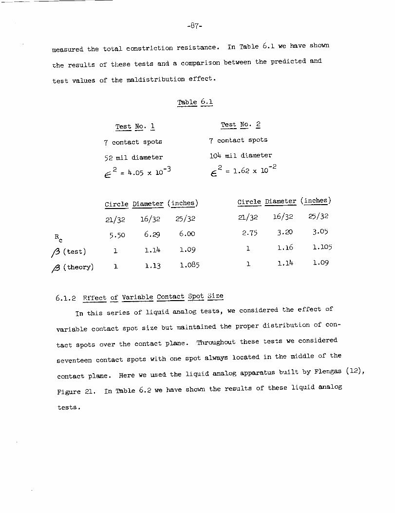
-87-
measured the total constriction resistance. In Table 6.1 we have shown
the results of these tests and a comparison between the predicted and
test values of the maldistribution effect.
Table 6.1
Test No. 1
7 contact spots
52 mil diameter
_2 : 4.o5 x 10-3
Test No. 2
7 contact spots
104 mil diameter
2= 1.62 x i0 -2
Circle Diameter (inches) Circl_____eDiameter (.inches)
21/32 16/32 25/32 21/32 16/32 25/32
R 5.50 6.29 6.00 2.75 3.20 3.05c
(test) 1 1.14 1.09 1 1.16 1.105
(theory) i 1.13 1.085 i 1.14 1.09
6.1.2 Effect of Variable Contact Spo____tSiz____ee
In this series of liquid analog tests, we considered the effect of
variable contact spot size but maintained the proper distribution of con-
tact spots over the contact plane. Throughout these tests we considered
seventeen contact spots with one spot always located in the middle of the
contact plane. Here we used the liquid analog apparatus built by Flengas (12),
Figure 21. In Table 6.2 we have shown the results of these liquid analog
tests.
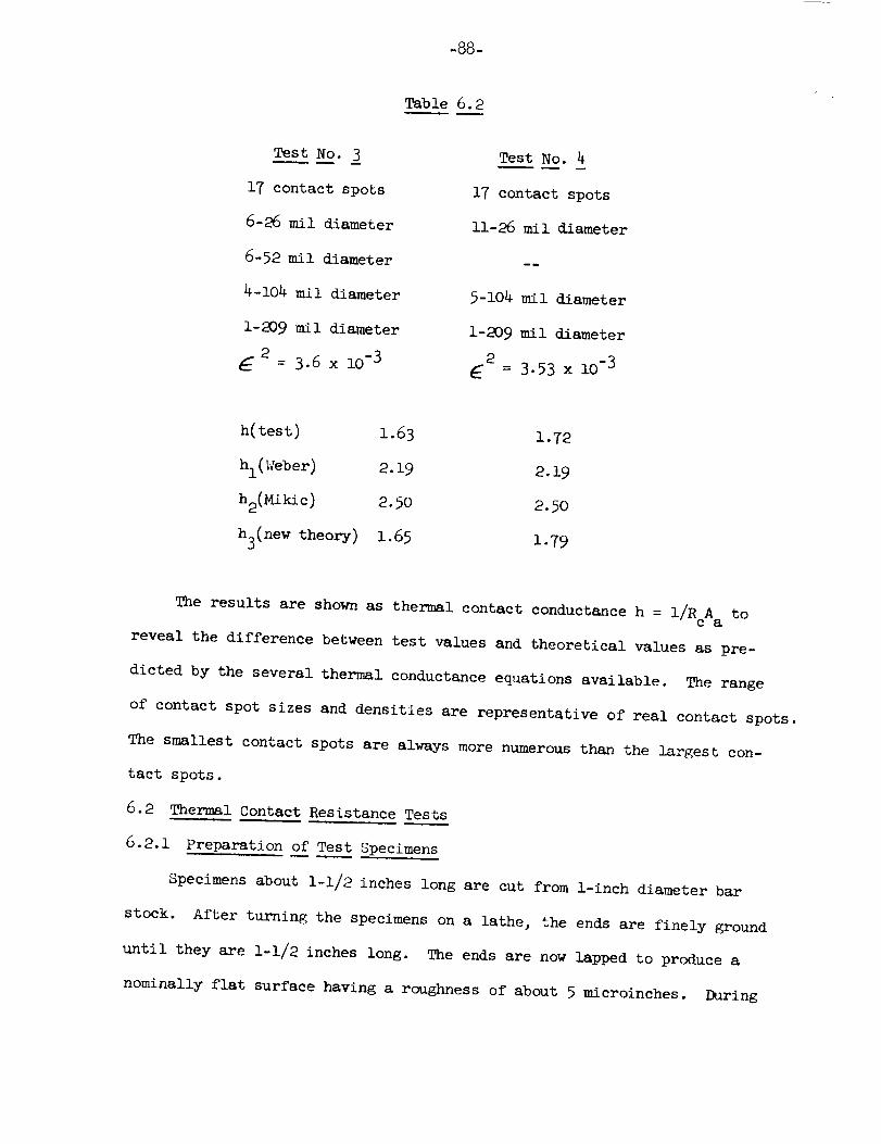
-88-
Table 6.2
Test No. 3
17 contact spots
6-26 mil diameter
6-52 rail diameter
4-104 rail diameter
1-209 mil diameter
_2 = 3.6 x i0 -3
Test No. 4
17 contact spots
11-26 mil diameter
--m
5-104 rail diameter
1-209 mil diameter
2E = 3.53 x lO-3
h(test) 1.63 1.72
hl(Weber) 2.19 2.19
h2(m_c) 2.50 2.50
h3(new theory) 1.65 1.79
The results are shown as thermal contact conductance h = I/R A toca
reveal the difference between test values and theoretical values as pre-
dicted by the several thermal conductance equations available. The range
of contact spot sizes and densities are representative of real contact spots.
The smallest contact spots are always more numerous than the largest con-
tact spots.
6.2 Thermal Contact Resistance Tests
6.2.1 Preparation of Test Specimens
Specimens about l-l/2 inches long are cut from 1-inch diameter bar
stock. After turning the specimens on a lathe, the ends are finely ground
until they are l-l/2 inches long. The ends are now lapped to produce a
nominally flat surface having a roughness of about 5 microinches. During
-90-
surfaces. The thermocouples (four in each specimen) are placed and
secured by means of Sauereisen. To insure proper alignment, the speci-
mens are placed in a holder which is removed once the specimens are loca-
ted in the test section. The holder keeps the specimens aligned (in
particular the wavy, rough surfaces) and insures there is no relative
slip between the surfaces. Having aligned the complete test section,
the vacuum chamber is closed, and a vacuum of about 5 x lO -6 mm Hg is
attained by means of the mechanical and diffusion pumps. At a nominal
pressure of 131 psi (determined by the load bellows), the heater is
turned on to produce an interface temperature of about 500°F. The sys-
tem and interface are permitted to outgas for about thirty-six hours.
After the outgassing has been accomplished, the heaters and cool-
ing syste_ are adjusted to give the desired heat flu_. The thermo-
couple readings are taken every half hour. After two identical succes-
sive readings, it is assumed that steady state conditions prevail. The
loads are increased by increments of about 500 psi until the maximum
load is obtained. The temperature at the interface is maintained rela-
tively constant by increasing the power to the heaters.
The results of tests performed with different materials and various
surface geometries are shown in tables and curves and will be discussed
in detail in Chapters 8 and 9.
6.3 Surface Deformation Tests
The specimens are prepared in exactly the same manner used in the
thermal contact resistance tests. Since the object of these tests was
to check the validity of the equation which predicts the relation between
the contour and Hertzian radius, two specimens were prepared having
-89-
the lapping process the surfaces are periodically checked for waviness;
the lapping process is continued until no waviness is present. For the
nominally flat, rough surface tests, the lapped surfaces are blasted
with glass beads with the apparatus shown in Figure 31. The surface
characteristics are obtained by means of the Talysurf. The prepared
specimens are stored in dessicators to prevent oxidationuntil they are
used in the heat transfer tests.
The _Bvy, rough surfaces are prepared in a slightly different manner.
After the lapping process, one end is made hemispherical by placing the
specimens in a lathe and spinning them at very high rpm against a polish-
ing cloth supported by a rigid, flat support. The cloth is covered with
varying coarseness polishing compounds, beginning with the coarse and
ending with the extremely fine compound. Because of the relative speeds
of the points on the surface, the points at the periphery wear more than
those located near the center. In this manner hemispherical waviness
can be generated. The out-of-flatness is now obtained by means of the
Talysurf. The surfaces are now blasted with the glass beads to produce
a rough, wavy surface. It is assumed that the waviness or out-of-flat-
ness is not drastically altered by the blasting process. The waviness
of the blasted surface is taken to be the same as the waviness before
blasting. As in the case of the nominally flat, rough specimens, the
wavy, rough specimens are stored in dessicators until used in the heat
transfer tests.
6.2.2 Vacuum Tests
The procedure for obtaining thermal contact resistance data is the
same whether the specimens have nominally flat, rough or wavy, rough
°91-
approximately the same_aviness. One specimenwas smooth, and the other
was bead blasted. It was determined by meansof the equation at what
nominal pressure there would be contact over the entire apparent area
for the wavy, rough surface. For the samenominal pressure, the smooth
surface would contact over a small fraction of the apparent area. The
bond paper is placed upon the rigid, flat smooth support. The carbon
paper is now placed face downupon the bond paper. One of the specimens
is placed on top of the carbon paper, and the system is placed in a holder
until loaded. The holder is removedafter a small load is placed on the
system. The desired load is placed on the system and held for a few
minutes. Upon removal of the load, the bond paper is examined to deter-
mine the extent of the region over which the specimens contacted. This
procedure showedqualitatively the effect of roughness upon the contact
of a wavy surface.
-92-
7. SURFACEPROFILEANALYSIS
7.1 Introduction
The mathematical analysis of the thermal contact resistance of many
small circular contact spots requires a knowledge of their number, size,
and spatial distribution. In the absence of surface waviness, only their
number and radii are necessary to determine completely their resistance
to heat transfer for the vacuum case. The surface deformation analysis,
for the completely plastic yielding of contacting asperities, requires
only a knowledge of the total real area of contact. Thus, it is seen
that in order to correlate thermal contact resistance (or conductance)
with the nominal contact pressure (or load, it is necessary that we
obtain information on the total real area and the number and radii of
all the contacts corresponding _o the surface geometry and the material
properties of the surface. In this analysis it is assumed that the sur-
faces do not have a dominant lay.
7.2 Surface Profile Theor_
There are two methods of measuring the surface topography. One
method employs optical techniques while the second method employs mechani-
cal means to probe the surface. In the first method a beam of collimated
light is projected at the surface, and then the diffuse reflected beam
is inspected by means of a photocell. Irregularities in the surface
appear as features in the reflected beam. This method does not damage
the surface being examined but is restricted by the wavelength of light
to surfaces which are rougher than 20 x lO -6 inches. The most widely
-93-
used method of measuring surface roughness employs a diamond stylus.
The surface is drawn under the stylus or the stylus is passed over the
surface. The vertical movements of the probe are amplified electronically
and recorded on a chart. It has been sho_m by Dr. J. B. P. Williamson
that with proper care even the softest metals can be probed_rith negligi-
ble damage to the surface. The performance characteristics are deter-
mined by the shape and size of the probe. The basic resolution in the
vertical direction is of the order of a microinch. Although it is highly
improbable that a single trace of a surface will reveal the highest points
of the traversed asperities, it is highly probable that the linear pro-
file does represent the surface to a high degree, in particular, the
spatial distribution of the asperities.
7.3 Number, Size, and Real Area of Contact Spots
Consider an arbitrarytraverse of length L across a surface. We
assume that the probed length L is a representative sample of the sur-
face and that the contact spots are distributed randomly over the nominal
contact area. When a nominally flat, smooth plane is brought into con-
tact with the representative profile, we note that the profile penetrates
the plane at a number of locations. It is also noted that the lengths
of the intersection vBry in magnitude. As the plane is moved closer to
the profile (simulating a load on the surface), the intersections increase
in number, and the variation in the incremental intersections becomes
more pronounced. For every trace through the surface at a particular
separation of the two planes, it can be shown from probability arguments
that the sum of the intersects per unit length of trace is proportional
to the real area ratio, Cooper (31),
N i. A2; •
ai=l
-94-
(7.1)
This statement is true for any trace as long as the trace length L is
representative of the surface.
If the real area is produced by the plastic deformation of the con-
tacting asperities, we can immediately write the relationship between
the nominal pressure, the yield pressure of the asperities, and the
measured quantity
N Ii
7__ _-=Pa/3_y (7.2)i=l
Following similar probability arguments, we can show that the num-
ber of contacts per unit apparent area can be written in terms of the
measured number of intersections per unit length of trace and the real
area ratio
A L _.a
Cooper (31) very elegantly showed that the number of intersections
per unit length of trace could be expressed as
N 2c.
L Aa
i=l
(7.4)
where the c. represents the radii of all the contact spots.1
-95-
We now recall that the thermal conductance Equation (3.7) forN
properly distributed contact spots is expressed in terms of Z ci/Aa"i=l
This means that the thermal conductance of a nominally flat, rough sur-
face can be obtained directly from a trace.
-96-
8. COMPARISON OF PREDICTED AND F_ERIM_AL RESULTS
8.1 Introduction
We shall in this chapter make a comparison between the published
studies and the present analysis in the light of the previously obtained
test data and the newly acquired experimental results.
8.2 Theoretical Heat Transfer Models
Almost all previously published analyses on thermal contact resist-
ance were based upon the assumption that the real area of contact con-
sisted of a large number of small equal size contact spots distributed
uniformly over the contact area whether it be the entire apparent area
or a fraction of the apparent area. The one major exception is the
macroscopic resistance theory proposed by Clausing (14). He states that
the macroscopic constriction effect is of importance and dominates the
thermal contact resistance of a majority of engineering surfaces. Clausing's
model is based upon the assumption that the apparent contact area can be
separated into a contact and noncontact region. In the noncontact region
there are few or no microcontacts while the contact region contains a
high density of microcontacts. He further assumes that the thermal resist-
ance of the macroscopic area is much greater than the pinching effect of
the microcontacts. He determines the macroscopic area by assuming it is
the result of elastic contact between hemispheres. As expected he found
good agreement between his theory and his test data; in particular, those
surfaces which were very smooth, very wuvy, and which had a high elastic
modulus. With aluminum specimens he had far less success; his theory
-97-
predicted thermal resistance orders of magnitude lower than actually
observed. Other investigators were even less successful in applying
his theory to their problems. This was especially true when the sur-
faces possessed roughness as well as waviness, and the nominal contact
pressures were in excess of lO00 psi. We conclude that Clausing's macro-
scopic constriction resistance theory is valid only under very restric-
tive conditions not generally met in industry.
Let us now return to the theories based on the pinching effect of
the contacting asperities. Some of the first attempts at predicting
contact resistance of rough surfaces in a vacuum were based on the
assumption that the constriction resistance of a single circular con-
tact spot is inversely proportional to the contact spot size (Weber solu-
tion). Assuming uniform distribution of equal size contact spots over
the apparent area, they obtained the following equation for the thermal
contact conductance
/N(cl2 2 22 km + c 2 + .... + aN (8.1)
hl(Weber) = Aa
We have written the conductance in this form so that it can be compared
with the other theories. Since the contact spots are all the same size,
the term under the square root is actually Nc.
More recently Mikic (Ii) and Roess (18) considered the effect of
the relative size of a single contact spot. They obtained a geometric
factor and applying it obtained a new expression for the thermal con-
ductance, again assuming equal size and uniform distribution,
-98-
_N( 2 2/Tk m cI + c2 + • • . CN2
h2 = Aa _ (8.2)
Equation (8.2) reduces to Eq. (8.1) in the limit when the contact spots
are very small.
We have proposed that both the actual sizes of the contact spots
as well as spot maldistribution must be considered in determining the
thermal contact conductance. Whenever the contact spots are properly
distributed, the thermal conductance can be written as
(Cl + °2 + .... %)h 3 - Aa _ (8.3)
but when maldistribution is also present to some degree, the conductance
wi ll be
_Z/_km (Cl//_ 1 + c2/_2 + .... CN/_N)
= • (8.4)A a
The liquid analog test results in Table 6.2 clearly demonstrate the
importance of the actual sizes of the contact spots. It is interest-
ing to note that the thermal conductance equation based on the Weber
solution overpredicts by 34 percent while the thermal conductance equa-
tion based upon a more realistic model overpredicts by 54 percent.
None of the previous theories considered maldistribution which can
reduce the thermal conductance even more. The liquid analog test results
in Table 6.1 show that this effect can be as large as 16 percent for a
moderately small amount of maldistribution.
-99-
When the contact spots appear as a number of clusters, and the
clusters are distributed over the apparent area, we have to propose
that the total resistance consists of the constriction resistance
based upon the size of the cluster (contour area) and the pinching
effect of the contact spots. Several investigators, notably Barkan (20),
Holm (21), Kragel'ski (29), and Greenwood (30), have proposed the follow-
ing expression for the thermal contact resistance of one cluster of
contact spots
e ____
1 1
-- - (8.5)
It is obvious that this is based on the Weber solution and is applica-
ble to a very special contact.
We have proposed the following expression which is based upon the
actual size of the contact spots and also takes into consideration the
relative size of the contact spots and also of the contour area
R i +
N cci
i=l
(8.6)
This equation reduces to the above equation in the limit that the
contact spots are very small, and the contour area is extremely small
relative to the apparent area. The equation agrees quite well with the
liquid analog test data obtained by Flengas (12). The geometric factor
_l for very small contact spots can be approximated by VT/16, but the
geometric factor _2 must be obtained from Figure (12) especially when _0.2.
-100-
8.3 Comparison of Models with Heat Transfer Data
In Figure 32 we have shown the heat transfer data plotted against
the nominal pressure on the interface. Although data were obtained for
several different materials, we have chosen to show only the data for
the stainless steel specimens. It can be seen that for a particular
nominal pressure the thermal contact conductance can differ by as much
as lO0 percent. This difference is due primarily to the difference in
the surface roughness. The smoother the surface, the greater the thermal
contact conductance appears to be the dou_inant feature of Figure 32.
We next plotted the same data in a slightly different manner to
show how strongly the thermal contact conductance depends upon the sur-
face geometry and the hardness of the material. We chose the surface
roughness and the slope of the asperities to be characteristic of the
surface and the yield strength under tensile loading to be characteris-
tic of the material. If we assume plastic deformation of the contact-
ing asperities, the ratio of nominal pressure to yield pressure can be
related to the area ratio E 2 Figure 33 shows the data plotted as a
2
thermal conductance number (_h/tan @ k ) versus the area ratio Em
It is interesting to note how well this correlates the test data over
the pressure range. It appears that for values of the area ratio exceed-
ing 2 x lO -3, all the data fall with a narrow band (_ 25 percent) on
a straight line having a slope of about 0.89 indicating that the con-
ductance is practically proportional to the nominal pressure. This
implies that the deformation of the asperities is most probably plastic
for the high loads. It is not surprising that we get such a good correla-
tion when it is realized that the parameter (_/tan @) is a measure of
-i01-
the size of the most probable contact. Since it does not change with
loading, the increase in the conductance must be due to the increase
in the number of contact spots. But it has been shown that the number
of contact spots is almost proportional to the nominal pressure (8).
For values of the area ratio below 2 x lO-3, the spread between
the data is muchgreater, and the slope is considerably less, about
0.49. It is believed that for nominal pressures below those corres-
ponding to _2 = 2 x lO-3, the contact is not strictly a contact between
nominally flat, rough surfaces. The waviness (which may not be detected
by examinations of linear profiles) may be present to some degree. If
the waviness were dominant, the slope of the data versus the load would
be about 0.33. Since the slope is actually between the slopes for com-
pletelywavyand nominally flat surfaces, we conclude that the contact
occurs over a contour area which is relatively large, but the pressure
distribution over the contour area produces many contacts near the center
of contact and fewer near the edge of the contact.
We have shown in Figure 34 the same test data used in Figure 33.
In this case we have used the equation developed by Mikic (ii) which is
based on the solution for an elemental heat channel, equal size contact
spots uniformly distributed over the apparent area, and plastic deforma-
tion of the contacting asperities. For all the test data for values of
the area ratio greater than 2 x 10 -3 , the theory predicts values greater
than observed. The discrepancy between theory and test data increases
with increasing load, and there can be as much as 125 percent difference
between the two values. It was believed that neglecting the variable
contact spot size and the spatial distribution resulted in the
-102-
discrepancy between theory and test data. It can also be seen in Figure
34 that the theory underpredicts for values of E2_ 2 x lO-3. As
noted above this is probably due primarily to the waviness effect, i.e.,
the pressure distribution over the contour area.
In Figure 35 we have shownhow the thermal contact conductance pre-
diction is affected by considering the variable contact spot size and
the maldistribution. The contact spot size variation can be determined
by examination oi' linear profiles. The maldistribution effect, however,
cannot be determined from the linear profiles. Wehave showna band of
the probable predicted values which is based upon assuming little or no
maldistribution for the smaller values of the area ratio and almost the
maximumcorrection for maldistribution for the very large values of the
area ratio. It is seen that the test data agree quite well with the
predicted band.
8.4 Surface Deformation Model____s
Several investigators have considered the effect of surface roug_h-
hess upon the contact between hemispheres (or spheres). Barkan (20)
showed experimentally that the contour size can be considerably larger
than the size predicted using the classical elasticity theory. He
showed that there can be contact because of the roughness beyond the
Hertzian radius. In his theory of contact resistance between hemispheres,
he assumed that the contour radius was always 1.7 times as large as the
Hertzian radius. Greenwood, et al., (27) developed a mathematical theory
which showed that the Hertzian results are valid at sufficiently high
loads, but at lower loads the effective pressure distribution is much
lower and extends much further than for smooth surfaces. They showed
-i03-
that the contour radius could be five times as large as the Hertzian
radius. Their equation is very difficult to use as it depends upon a
complex iterative procedure. For the example considered in their paper,
we were able to show that their theory and ours are approximately the
same. The other investigator is Goodman(28) who considered the con-
tact stress of normally loaded rough spheres. His analysis did not
result in an equation which would predict the contact region as a func-
tion of the surface geometry, the material properties, and the applied
load. In one figure he showedthat for low contact loads, the observed
compliance at the origin _as smaller than predicted using the Hertz
theory. This corresponds to the fact that since the load is distribu-
ted over a larger region, the pressure at the origin is _uch smaller,
and hence the compliance at the origin will be smaller.
-lo4-
9. CONCLUSIONS
9.1 Discussion of Results
It has been shown that the temperature of the microcontacts is uni-
form and equal for all microcontacts irrespective of their shape, rela-
tive size, or spatial distribution. It has also been shown that the
total apparent area is subdivided among the microcontacts according to
their size (radius). Every microcontact in the total field of microcon-
tacts contributes towards determining what portion of the total apparent
area corresponds to a particular microcontact. A thermal contact resist-
ance equation was developed for appropriately distributed microcontacts.
It was seen that the resistance is inversely proportional to the sum of
the radii of all the microcontacts. Theequation agreed extremely well
with liquid analog tests.
It was next shown that a single microcontact could be maldistribu-
ted within its corresponding apparent area. The maldistribution effect
is more apparent with relatively large microcontacts, but the maximum
change in the constriction resistance appeared to be about _-2whenever
the microcontact was displaced to the boundary of the heat flux tube.
We were able to correlate the maldistribution effect with the relative
size and relative displacement of the microcontact by postulating that
the distance between the isothermal surfaces which bound the disturbed
temperature region is proportional to the difference between the radii
of the corresponding apparent area and the microcontact. The maldistribu-
tion effect appears as a reduction in the effective size of a maldistributed
microcontact. The theory was compared with liquid analog tests, and the
agreement was excellent.
-lO5-
It was next assumed that the thermal resistance of a wavy, rough
contact was due to two resistances which could be added linearly. This
result is based upon the assumption that there exist three isothermal
planes: one in the plane of contact, one a small distance from the con-
tact plane, and one a large distance away. When no waviness is present,
the second and third planes are coincident, and there is no waviness resist-
ance. This assumption was checked with liquid analog tests and proved
to be an accurate description of the real situation.
The surface deformation analysis showed that the surface roughness
can have a significant influence upon the deformation of an hemispheri-
cal surface. When the loads are light and the surface roughness large,
the contour radius can be five times as large as the Hertzian radius.
For sufficiently large nominal pressures, the contour radius is identi-
cal to the Hertzian radius, and the pressure distribution over the con-
tact area is the Hertzian pressure distribution. The theory agreed qualita-
tively with test data for the conditions that were examined.
The thermal analysis and deformation analysis agreed with the thermal
contact resistance data. In particular, the theory showed that the assump-
tion of plastic deformation of contacting asperities is valid after the
entire apparent area has come into contact. The thermal analysis showed
why the previously developed theories overpredict the thermal contact con-
ductance at large nominal pressures.
9.2 Recommendations for Future Research
It is recommended that further work be done to extend the concept
of size effect and appropriate distribution to contacts made in a fluid
-lO6-
environment. The author recommends that a study be undertaken to see
whether the basic concept of an as3nmetric heat flux tube can be extended
to include the wavy, rough contact. A preliminary study along these
lines resulted in an equation which had the same shape as the liquid
analog test data, but underpredicted the thermal resistance by about 30
percent.
It is also recommended that the surface deformation of rough, wavy
surfaces be compared with heat transfer data for nominal pressures in
the 1 to 50 psi range. In this pressure range the surface roughness has
significant influence upon the material deformation and upon the thermal
resistance •
This work considered the case of bead-blasted hemispherical surfaces
in which there were no lay. It is recommended that the thermal and
deformation analyses be performed upon surfaces which have a predominant
lay.
-io7-
BIBLIOGRAPHY
Section l: M.I.T. Theses
1. Fenech, Henri, "The Thermal Conductance of Metallic Surfaces in Con-
tact," M.I.T. Sc.D. Thesis, May, 1959.
2. Henry, John Jewett, "Thermal Resistance of Metals in Contact," M.I.T.
M.S. Thesis, August, 1961.
3- Carroll, Tom Wentworth, "Statistical Calculation of Geometric Parame-
ters for Semi-Smooth Contiguous Surfaces," M.I.T.M.S. Thesis, Janu-
ary, 1962.
4. Kaszubinski, Leonard Joseph, "DeterT_nation of the Number of Contacts
Between Two Surfaces Pressed Together," M.I.T.M.S. Thesis, August,
1963.
5. Velissaropoulos, Pandelis D., "Apparatus for Measurement of Contact
Resistance," M.I.T.M.S. Thesis, August, 1963.
6. Horn, Stefau Schulze, "Thermal Contact Resistance of Graphite," M.I.T.
M.S. Thesis, September, 1963.
7. Flamm_ng, Dennis Craig, "The Use and Comparison of Autoradiographi-
cal and Statistical Methods of Determining the Number of Contacts
Between Two Surfaces Pressed Together," M.I.T.B.S. Thesis, June 1963.
8. Foster, Edward Terence, "Prediction of Contact Population in Bimetallic
Surface Junctions," M.I.T.M.S. Thesis, August, 1964.
9- Henry, John Jewett, "Thermal Contact Resistance," M.I.T. Sc.D. Thesis,
August, 1964.
Yovanovich, M° M., "Thermal Contact Conductance in a Vacuum," M.I.T.
M.E. Thesis, February, 1966.
10.
-lO8-
Ii. Mikic, B. B., "Thermal Contact Resistance," M.I.T. Sc.D. Thesis,
September, 1966.
12. Flengas, S., "Analog Study of Thermal Contact Resistance for Wavy
and Rough Surfaces," M.I.T.M.S. Thesis, June, 1967.
Section 2: Other Contact Resistance References
13. Cordier, H., "Experimental Study of the Influence of Pressure on
Contact Thermal Resistance," Redstone Scientific Information Center,
(RSIC - ll6) 1961. (Translated from Acad. des Sciences, Compts.
Rendus 250, April 25, 1960.)
Clausing, A. M. and Chao, B. T., "Thermal Contact Resistance in a
Vacuum Environment," University of Illinois, ME-TN-242-1, August,
1963.
Clausing, A. M., "Some Influences of Macroscopic Constrictions on
Thermal Contact Resistance," University of Illinois, ME-TN-242-2,
April, 1965.
Weber, H., "Ueber Bessel'sche Functionen und ihre Anwendung auf
die Theorie der elektrischen Strome," Crelle, Bd. 75, 1873. See
reference (17).
Gray, A. and Mathews, G. B., A Treatise on Bessel Functions and
Their Applications to Physics," Dover Publications, Inc., New York,
1966.
Roess, L. C., "Theory of Spreading Conductance," Appendix A of an
unpublished report of the Beacon Laboratories of Texas Company,
Beacon, New York.
Carslaw, H. S. and Jaeger, J. C., Conduction of Heat in Solids,
London: Oxford University Press, Second Edition, 1959.
14.
15.
16.
17.
18.
19.
-lO9-
"A20. Barkan, P. and Tuohy, E.J., Contact Resistance Theory for Rough
Hemispherical Silver Contacts in Air and in Vacuum," IEEE Trans. on
Power Apparatus and Systems, Vol. PAS-8_, No. 12, December 1965.
21. Holm, R., Electric Contacts Handbook, Springer-Verlag,
Berlin/Gottingen/Heidelberg, 1958.
Section 3: Subjects Pertinent to Contact Resistance
22. Rabinow-icz, E., "A Quantitative Study of the Wear Proeess," Proceed-
ings of the Physical Society, B, Vol. LXVI, 1953.
23. Love, A. E. H., Th___eMathematical Theory of Elasticity, Dover Publica-
tions, Inc., New York, 1944.
24. Timoshenko, S. and Goodier, J. N., Theory of Elasticity, McGraw-Hill
Book Company, Inc., New York, 1951.
25. Greenwood, J. A., "On Area of Contact Between Rough Surfaces and
Flats," A.S.M.E. Paper No. 65-Lub-lO, 1965.
26. Greenwood, J. A. and Williamson, J. B. P., "Contact of Nominally
Flat Surfaces," Proc. Roy. Soc., A, vol. 295, 1966.
27. Greenwood, J. A. and Tripp, J. H., "The Elastic Contact of Rough
Spheres," A.S.M.E. Paper No. 66-WA/APM-28, 1966.
28. Goodman, L. E., "Contact Stress Analysis of Normally Loaded Rough
Spheres," Jour. of Appl. Mech., pp. 515-522, September, 1962.
29. Kragel'ski, IV. and Demkin, N. B., "Contact Area of Rough Surfaces,"
Wear, Vol. 3, PP. 170-187, 1960.
30. Greenwood, J. A., "Constriction Resistance and the Real Area of
Contact," Brit.J. Appl. Phys., Vol. 17, 1966.
31. Cooper, M. G., "Interfacial Contact Resistance: Some Mathematical
Notes," M.I.T. Report.
-llO-
APPENDIX A
CONTACT SPOTS ARE ALL ISOTHERMAL
When the contact spots lie in a surface which, if there were com-
plete physical contact, is an isothermal surface, then the actual con-
tact spots are at a uniform and common temperature irrespective of
their relative shape and size, their distance from each other, and
the thermal conductivities of the materials forming the contact.
Let us consider a typical heat channel which consists of two
materials of different thermal conductivities touching only at two
circular (the argument is not dependent upon the shape of the contact
spot) contact spots having different radii, Figure i0.
The apparent contact area A a consists of two regions: the non-
contacting area Ab and the contacting area Ac. Let us assume Ab is
thermally insulated; i.e., _ T/_ n = 0 over A b. This is true only
in the limit when there is a perfect vacuum in the voids and the radia-
tion transfer across the voids is negligible. Over A there will bec
heat transfer, and we assume that each contact spot is uniform in tem-
perature. (It is intuitively difficult to believe that radial heat
transfer can exist in the plane of the contact.)
Far upstream of the contact plane, there will exist a surface 1
with constant temperature v I. The heat flux over 5his surface is uni-
form, and the quantity of heat which passes through this surface in
unit time is Ql" Similarly far downstream of the contact plane, there
will exist a surface 3 with constant temperature v 3. Here also the
heat flux is uniform, and the heat which flows through the surface in
-iii-
unit time is Q3" All other bounding surfaces are defined by heat flow
lines and are, therefore, thermally insulated; i.e., _T/_n = 0 every-
where. In the absence of sources or sinks within the defined boundaries,
QI = Q3"
Let us assume that one contact spot is several times larger than
the second contact spot and that they are at some finite distance apart.
They are in thermal communication with either isothermal surface 1 and
3 and with each other through the two solids having thermal conductivi-
ties kI and k2, where k I = k 2. There is no thermal communication between
the contact spots in the contact plane, i.e., through the plane of Ab.
Let the larger contact spot with radius cI have uniform tempera-
ture v' and the smaller contact spot vith radius c2 have the uniformcl'
temperature v' where v' v' A certain quantity of heat _clWillc2' cl _ c2"
flow in unit time between the surface 1 and the larger contact spot.
This quantity of heat will be dependent upon the temperature difference
(vI - V_l) and the total therm_l resistance Rlt I to heat flow between
the two isothermal planes. The total resistance Rlt I is the sum of
two thermal resistances, the bulk resistance Rlml, and the constric-
tion resistance due to the contact spot Cl; i.e., Rlt I = Rlml + Rlcl"
Similarly the heat flow per unit time between surface 1 and the second
contact spot will be ' and it also will depend upon the temperatureQlc2'
T
difference (vI - Vc2) and the total resistance Rlt 2 = Rlm2 + Rlc2"
The heat which flows across surface i must flow through the contact
spot; i e., QI Qlcl + '• = Qlc2" Following the same reasoning, it can
be shown that the heat which passes through the contact spots must
flow through surface 3; i.e., Q'ic3 + = Q3 The net heat flowQ2c3
-112-
per unit time between the larger contact spot and surface 3 is Q{c3
which depends upon V'cl - v3 and Rlt 3 = Rim3 + Rlc 3. Also, the net
heat flow per unit time between the smaller contact spot and surface
3 is Q2c3'with corresponding temperature difference V'c2 - v3 and total
resistance R2t3 = R2m3 + R2c3-
Since we assumedthat the temperature of the larger contact spot
is greater than the temperature of the smaller contact spot, there
will be heat flow between the contact spots. The quantity of heat
flowing per unit time will depend upon the temperature difference
' - v_2) and the thermal resistance between these two contact spots.(Vcl
The heat flow through solid 1 will be QII2 = (Vcl - Vc2)/Rll2 and
!
through solid 2 will be Q122 = (V'cl - Vc2)/R122" Qll2 need not be
equal to Q122 as Rll 2 need not be equal to R122. Figure36shows the
quantities of heat exchanged between the various isothermal surfaces
and the corresponding thermal resistances.
Let us assume that the two contact spots are at uniform tempera-
tures Vcl and Vc2 , respectively, where Vcl_V'cl and Vc2 _ V'c2 and
also Vcl = Vc2. In the light of the previous discussion, the heat
flows become Qlcl_ O'Icl and Qlc3 _ 0'_Ic3for the larger contact spot,
and Qlc2_ Q{c2 and Q2c3 _ Q2c3 for the smaller contact spot. Since
Vcl = Vc2 , the net flow of heat between the contact spots through either
solid goes to zero; i.e., QII2 = Q122 = O.
Let us now consider the steady-state heat transfer per unit time
through two control surfaces completely surrounding either contact spot.
One can determine the following two heat balances for the case of unequal
contact spot temperatures
-113-
T
- Qicl + QII2 + Q122 + Qlc3 0(A.1)
- Q_c2 - QII2 - Q122 + Q2c3 = 0(A.2)
Adding and transposing terms result in
2(%12+ %22) : (Qiol- Qic3) " (Qia2- Q_o3) (A.3)
Since Qicl _ Qlcl and Qic3 _ Qlc3' one can write (Qicl - Qic3 )< (Qlcl - Qlc3 )'
and similarly one can write - (Qic2 - Q2c3 )_ - (Qlc2 - Q2c3 )"
Equation (A.3) can now be rewritten in quantities which relate
the heat flow between contacts to the heat flow into and out of each
contact spot under steady-state conditions.
2(QI12 + Q122 ) _ (Qlci - Qlc3 ) - (Qlc2 - Q2e3 ) (A.4)
For steady-state conditions and equal contact spot temperatures, the
total heat flow per unit time into and out of the control surfaces
must be equal
Qlcl + QIc2 = QIc3 + Q2c3 (A.5)
which can be rewritten as
(QIc2 - Q2c3 ) = (QIc3 - Qlcl ) (A.6)
Substituting Eq. (A.6) into (A.4), one obtains the following relation-
ship.
QII2 + Q122 _ _Icl " QIc3 = O (A.7)
-i14-
This inequality can only be satisfied if one or the other quantity is
negative_ i.e., the heat flow takes place in a direction which is oppo-
site to the assumed direction. This would require that the tempera-
ture of one contact spot be greater than the other when considering
heat flow in one solid and that the temperature inequality be reversed
when considering heat flow in the second solid. This is physically
impossible, and, therefore, the two contact spot temperatures must be
identical.
The argument can be extended to include a third contact spot lying
in the same plane and having yet another size quite different from the
sizes of the other two spots. It can be shown that Vcl = Vc2 = Vc3.
By inductive reasoning it can be shown that the temperature of all the
contact spots must be the same value independent of the contact spot
shape, size, distance between contacts, and the quantity of heat flow-
ing through the spot. The assumption of equality of contact spot tem-
perature is valid whether the materials forming the contact have equal
thermal conductivities or not. This argument can now be used to prove
the assumption that the temperature over the contact spot is uniform.
A uniform temperature over a circular contact spot requires a parabolic
heat flux distribu5ion over the contact spot.
In this analysis it was assumed that the isothermal planes were
flat and parallel to the contact plane. The adiabatic w_lls of the
heat channel were defined by the outermost heat flow lines which pass
through the contact and are assumed to be parallel. Two special cases
arise in which the isothermal planes and contact plane are not flat
and the adiabatic heat channel walls are not parallel. Figure ii
-n5-
shows either the case for coaxial cylinders or concentric spheres.
The inner surface is isothermal at temperature v l, and the outer sur-
face is isothermal at temperature v2 where Vl_ v2. The broken sur-
face represents either a coaxial cylinder or a concentric sphere. If
there were perfect contact along this surface, it would be an iso-
thermal surface. Based on the arguments developed for flat surfaces,
we can assume that contact spots distributed on this surface will be
uniform in temperature and will all be at the same temperature inde-
pendent of their shape, size, distribution, and magnitude of the heat
flow through the contact spots and the thermal conductivities of the
materials on either side of the contact surface.
-116-
APPENDIXA
ALTERNATEARGUMENT
Consider the contact problem shown in Figure 37, which shows
two unequal sized contact spots transferring all the heat which flows
between isothermal surfaces i and 2 which are parallel to the contact
plane and the samedistance from the plane. There is no flow of heat
through the bounding walls of the heat channel and none through the
contact plane beyond the contact spots. Let the broken lines indicate
the heat flux tubes feeding heat to the contact spots. By definition
no net heat will flow across the commonboundary.
Separate the problem shownin Figure 37 into two sections at the
contact plane as shownin Figure 37. The two sections are coupled
by the fact that the temperature of the smaller contact spot a and a'
must be the same, and the heat flow out of a must be equal to the heat
flow in a'. Similar statements can be made concerning contact spot b
and b'. Assume isothermal surface I is at temperature I while iso-
thermal surface 2 is at temperature 0 and that the thermal conductivi-
ties of the two sections are identical. Further assume that the thermal
conductivity is independent of the temperature.
Consider the heat transfer problem through contact spot 2 (the
larger one). In the upper section one can write that Q2 = (I - b)/R 2
where R2 is the thermal resistance of heat flux 2 in the upper section.
A similar expression can be _ritten for the lower section, Q2 = (b' - O)/R_.
The thermal resistance is directly proportional to the normal flow area
and the distance through which the heat flows. _;e assume that there is
-117-
symmetry of heat flow about the contact plane; i.e., the heat flow
pattern in the heat flux tube 2' is the mirrorimage of the heat flow
pattern in heat flux tube 2. From this we conclude that the total
thermal resistances of the heat flux tubes 2 and 2' are identical;
i.e., R2 = R_. Thenb + b' = i. Since b = b', b = b' = 0.5.
Wenow consider heat flux tubes 1 and i'. In the upper section
the heat flow is related to the thermal resistance R1 and the tempera-
ture difference (1 - a) by Q1 = (i- a)/RI. Similarly for the lower
section, Q1 = (a' - O)/R_. Since the heat flow pattern in the heat
flux tubes feeding contact spot 2 is identical in sections 1 and 2,
we conclude that the heat flow pattern in the heat flux tube feeding
= ' Therefore,contact spot 1 is identical. This meansthat R1 R1.
a + a' = 1 from the coupling of Ql' But a = a', and this meansthat
a = a' = 0.5, the sameas the larger contact spot.
The argument can be extended to contacts which consist of dissimi-
lar materials; i.e., the thermal conductivities are unequal. The
assumption of heat flow symmetryabout the contact plane is still valid.
It can be shownthat the temperatures of the contact spots are equal
but that because of the different thermal conductivities, their levels
will be higher or lower than the value determined for identical thermal
conductivities.
The assumption of heat flow symmetrywill always be true if there
is perfect contact.
-I18-
APPENDIXB
ASYMMETRICHEATFLUXTUBE
Whenthe definition of an elemental heat flux tube was established,
it was noted that the existence of an asymmetric contact was possible.
The asymmetric contact was defined as that contact spot whoseaxis of
symmetry is not coincident with the axis of the elemental heat flux
tube. Weask the following questions:
1. )_at is the effect of asymmetry on the contact resistance?
2. Howdoes the relative size of the contact spot affect the change
in the congact resistance?
Ideally we should resolve this problem by finding solutions to
Laplace's equation which satisfy the appropriate boundary conditions.
Since by definition there is no axis of symmetry, the solution will
depend upon three coordinates. The problem is not amenable to a rigor-
ous mathematical approach, and, therefore, we must resort to someengi-
neering approximations.
First, let us establish the fact that _he temperature of the con-
tact spot is uniform irrespective of its relative size (E), its shape
(we assumecircular contacts), and its asymmetry. Consider a small
circular contact spot which lies near the boundary of the elemental
heat flux tube. There is no heat transfer in the regton outside the
contact spot. All the heat passing through an isothermal plane some
distance above the contact flows through the contact spot and out
through another isothermal plane somedistance below the contact spot.
The heat flow pattern on either side of the contact spot will be
-ll9-
identical, and the isotherms will have the same spacing if the thermal
conductivity on either side of the contact is the same. If the thermal
conductivities are not the same, the heat flow pattern on either side
will still be the same, but now isotherms will not have the same spac-
ing on both sides of the contact. The only way that the flow pattern
and temperature distribution can be satisfied on both sides of the con-
tact is to have a uniform temperature over the contact spot.
The potential problem has now been reduced to a three-dimensional
region bounded by an isothermal plane, adiabatic walls, and a second
plane which consists of a small circular isothermal spot surrounded by
an adiabatic region, Figure 15. This represents one half of the asym-
metric problem. The region between the two planes is the region of
three-dimensional temperature distribution. Heat passing between the
isothermal planes experiences a resistance to flow. The total resist-
ance can be separated into the material resistance and the constric-
tion or contact resistance.
It was shown earlier for the symmetric contact that when the con-
tact spot is very small (E_<I), the distance from the contact plane
to the isothermal plane is equal to the radius of the lemen_al heate J-
flux tube. It is obvious that as the size of the contact spot increases,
the isothermal plane will approach the contact plane, and in the limit
when the contact spot fills the conbact plane (6_ i), the isothermal
plane will be coincident with the contact plane. This implies that
as the contact spot becomes larger the disturbed temperature region
becomes thinner, Figure 14. As a first approximation assume that the
distance between the contact plane and the isothermal plane is linearly
-120-
related to the difference between the heat flux tube radius and the
contact spot radius; i.e., g/b = (1 - E). This relation satisfies
the limiting values of E and probably gives a good approximation for
intermediate values of 6.
The effect of asymmetrywill be resolved by using the concept of
thermal resistance as a function of the flow area and the flow path.
The total resistance will be an integrated value of the elemental
resistance between the isothermal planes. It is obvious that the
optimum situation occurs when the contact is symmetric; i.e., the
integrated value of the combinatLon of flow area and flow path is a
minimum, and hence the resistance is a minimum. Whenthe contact spot
is displaced from its symmetric position, the flow area and the path
are both changed, and it is expected that the integrated value should
be larger. The maximtunvalue will occur when the contact spot has
been displaced to within a contact spot radius of the boundary. For
each displaced position of the contact spot, there will be a differ-
ent value for the resistance. If we assumethat the integrated flow
area does not change significantlybetween the symmetric and maximum
asymmetric cases for all contact sizes, then the resistance will be
proportional to the integrated flow path. As a first approximation
assumethat the integrated flow path can be represented by the straig_ht
line joining the center of the contact spot, Figure 15. The total
resistance at any displaced position _ relative to the total resist-
ance for the symmetric case can be written asi
-: + )-2j
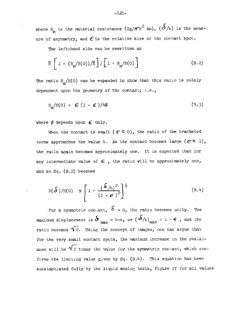
-121-
where R is the material resistance (2g/y['b 2 kln), (_/b) is the meas-m
ure of asymmetry, and E is the relative size of the contact spot.
The left-hand side can be rewritten as
The ratio Rm/R(O ) can be expanded to show that this ratio is solely
dependent upon the geometry of the contact; i.e.,
Rm/ (O) : & (1 - E (B.3)
where ¢ depends upon E only.
When the contact is small (EGO), the ratio of the bracketed
terms approaches the value 1. As the contact becomes large (_:_ 1),
the ratio again becomes approximately one. It is expected that for
any intermediate value of 6 , the ratio will be approximately one,
and so Eq. (B.2) becomes
R(_)/R(O) _ I I + (l(_/b)2I_--E )2
For a symmetric contact, _ = O, the ratio becomes unity.
maximum displacement is _ max J/b)max= b-c, or ( = i -
ratio becomes _.
(B.4)
The
, and the
Using the concept of images, one can arg_ae that
for the very small contact spots, the maximum increase in the resist-
ance will be _2 times the value for the symmetric contact, which con-
firms the limiting value given by Eq. (B.4). This equation has been
substantiated fully by the liquid analog tests, Figure 17 for all values
-122-
of E and the range of _/b. Equation (B.4) can be rewritten to give
the maximumasy_netry allowable for a particular value of the ratio
R(J)/R(O)
1
(S/b) = (1 - _) (R(g)/R(O)) 2 - 1 (B._)
It is seen that the small contacts can be displaced a large dis-
tance from the symmetric position before there is a significant increase
in the resistance. This means that the small contact spots are rela-
tively insensitive to the boundary of the heat flux tube; i.e., the
boundary could have the shape shown in Figure 19, and the assumption
of a circular heat flux tube is a very good approximation. The large
contact spots are very sensitive to the boundary of the heat flux tube,
and a relatively small displacement is reflected in a large change in
the resistance.
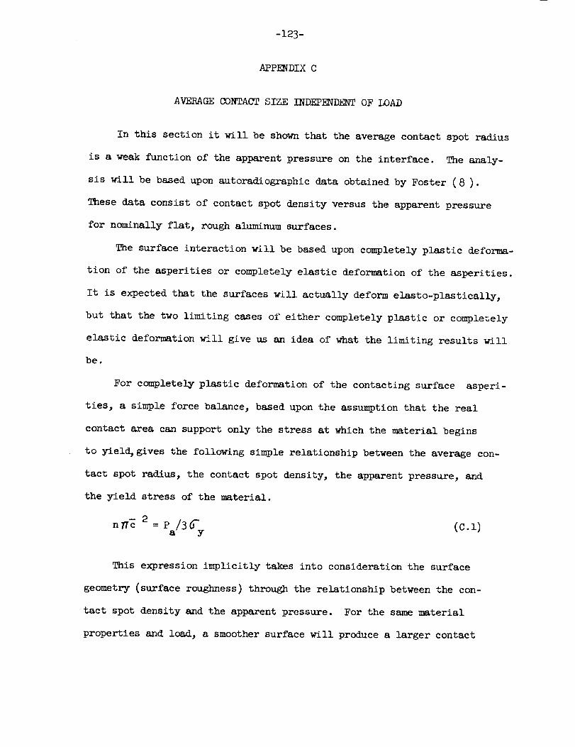
-123-
APPENDIX C
AVERAGE CONTACT SIZE INDEPENDENT OF LOAD
tact spot radius, the contact spot density,
the yield stress of the material.
In this section it will be shown that the average contact spot radius
is a weak function of the apparent pressure on the interface. The analy-
sis will be based upon autoradiographic data obtained by Foster (8).
These data consist of contact spot density versus the apparent pressure
for nominally flat, rough aluminum surfaces.
The surface interaction will be based upon completely plastic deforma-
tion of the asperities or completely elastic deformation of the asperities.
It is expected that the surfaces will actually deform elasto-plastically,
but that the two limiting cases of either completely plastic or completely
elastic deformation will give us an idea of what the limiting results will
be.
For completely plastic deformation of the contacting surface asperi-
ties, a simple force balance, based upon the assumption that the real
contact area can support only the stress at which the material begins
to yield, gives the following simple relationship between the average con-
the apparent pressure, and
nD'_ 2 = Pa/3G (C.l)
This expression implicitly takes into consideration the surface
geometry (surface roughness) through the relationship between the con-
tact spot density and the apparent pressure. For the same material
properties and load, a smoother surface will produce a larger contact
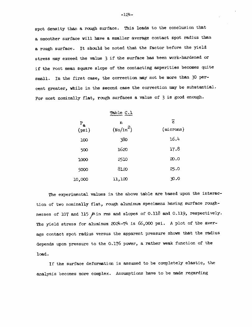
-124-
spot density than a rough surface. This leads to the conclusion that
a smoother surface will have a smaller average contact spot radius than
a rough surface. It should be noted that the factor before the yield
stress may exceed the value 3 if the surface has been work-hardened or
if the root mean square slope of the contacting asperities becomes quite
small. In the first case, the correction may not be more than 30 per-
cent greater, while in the second case the correction may be substantial.
For most nominally flat, rough surfaces a value of 3 is good enough.
Table C.1
Pa n c
(psi) (No/in 2) (microns )
too 38o 16.4
5OO ]_62O 17.8
i000 2510 20.0
5000 8120 25.0
i0, OOO ii, 120 30.0
The experimental values in the above table are based upon the interac-
tion of two nominally flat, rough aluminum specimens having surface rough-
nesses of 107 and ll5 _in rms and slopes of O.118 and O.119, respectively.
The yield stress for aluminum 2024-T4 is 66,000 psi. A plot of the aver-
age contact spot radius versus the apparent pressure shows that the radius
depends upon pressure to the 0.176 power, a rather weak function of the
load.
If the surface deformation is assumed to be completely elastic, the
analysis becomes more complex. Assumptions have to be made regarding
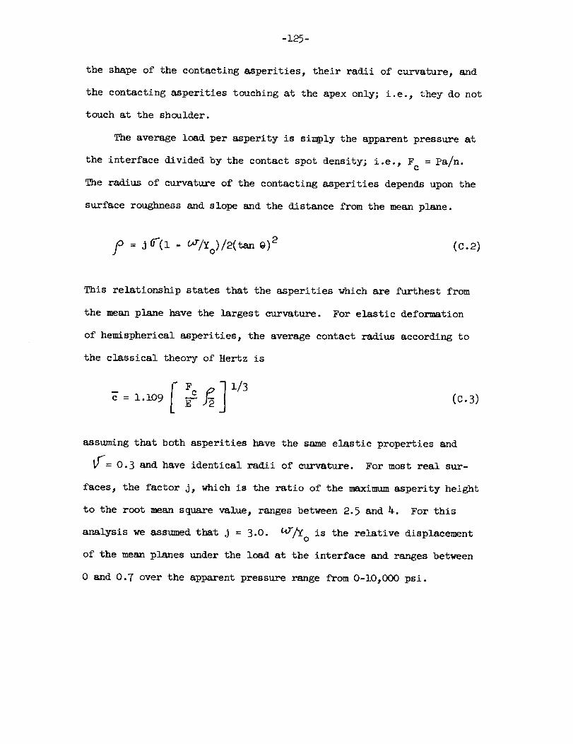
-125-
the shape of the contacting asperities, their radii of curvature, and
the contacting asperities touching at the apex only; i.e., they do not
touch at the shoulder.
The average load per asperity is simply the apparent pressure at
the interface divided by the contact spot density; i.e., F c = Pa/n.
The radius of curvature of the contacting asperities depends upon the
surface roughness and slope and the distance from the mean plane.
p : j - Q)2 (c.2)
This relationship states that the asperities which are furthest from
the mean plane have the largest curvBture. For elastic deformation
of hemispherical asperities, the average contact radius according to
the classical theory of Hertz is
_ Ec = 1.109 _-- (C.3)
assuming that both asperities have the same elastic properties and
_= 0.3 and have identical radii of curvature. For most real sur-
faces, the factor j, which is the ratio of the maximum asperity height
to the root mean square value, ranges between 2.5 and 4. For this
analysis we assumed that j = 3.0. _//Yo is the relative displacement
of the mean planes under the load at the interface and ranges between
0 and 0.7 over the apparent pressure range from O-lO,O00 psi.
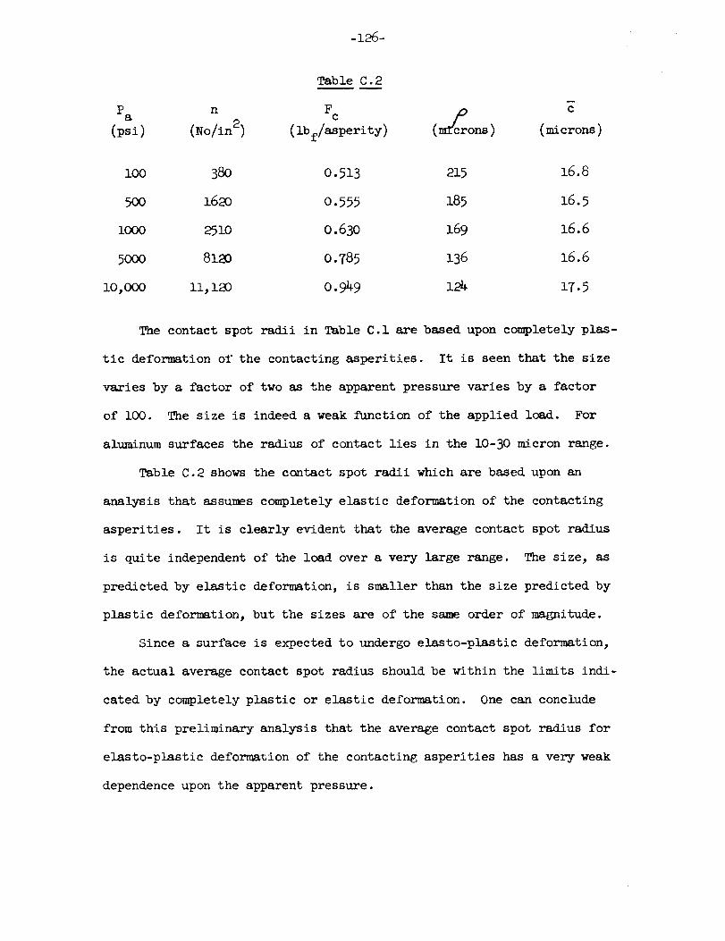
-126-
Table C.2
Pa n Fc(No/in 2) (lbf/asperity) (m_crons) (microns)(psi)
i00 380 O. 513 215 16.8
500 1620 O. 555 185 16.5
i000 25 i0 O. 630 169 16.6
5000 8120 O. 785 136 16.6
i0,000 ii, 120 O. 949 124 17.5
The contact spot radii in Table C. 1 are based upon completely plas-
tic deformation of the contacting asperities. It is seen that the size
varies by a factor of two as the apparent pressure varies by a factor
of lO0. The size is indeed a weak function of the applied load. For
aluminum surfaces the radius of contact lies in the 10-30 micron range.
Table C.2 shows the contact spot radii which are based upon an
analysis that assumes completely elastic deformation of the contacting
asperities. It is clearly evident that the average contact spot radius
is quite independent of the load over a very large range. The size, as
predicted by elastic deformation, is smaller than the size predicted by
plastic deformation, but the sizes are of the same order of magnitude.
Since a surface is expected to undergo elasto-plastic deformation,
the actual average contact spot radius should be within the limits indi-
cated by completely plastic or elastic deformation. One can conclude
from this preliminary analysis that the average contact spot radius for
elasto-plastic deformation of the contacting asperities has a very weak
dependence upon the apparent pressure.
-127°
It should be borne in mind that for any particular load and surface
geometry, there will be a spectrum of contact spot sizes. The avers_e
contact spot size represents the largest percentage of actual contacting
asperities. It is as yet unknown what the maximum contact spot could be
produced, and it is believed that the minimum size may be related to the
surface energy of the contacting asperities (22). As the load is increased,
the total number of contacting asperities increases, and although the
average contact spot size increases very little, the range of contact
spot size increases.

-128-
APPENDIX D
HEAT TRANSFER DATA
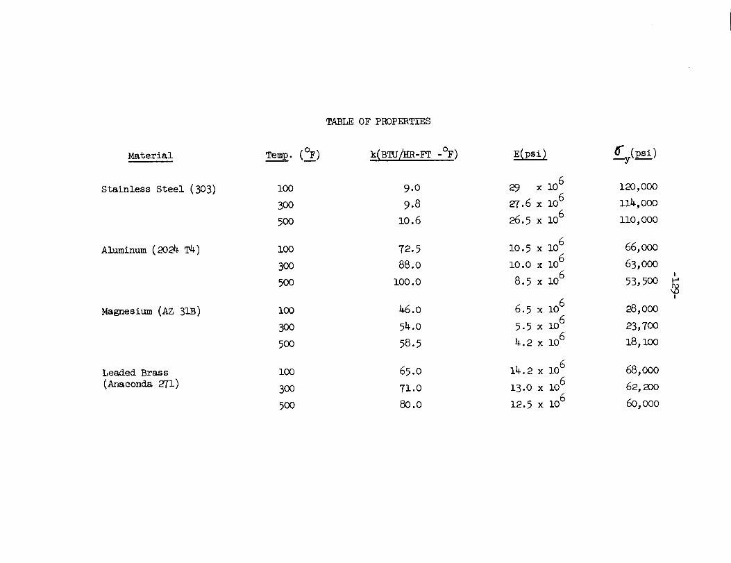
TABLEOFPROPERTIES
Material
Stainless Steel (303)
Aluminum (2024 T4)
Magnesium (AZ 31B)
Leaded Brass
(Anaconda 271)
Temp.(OF)
lO0
3oo
500
lO0
BOO
5OO
lO0
Boo
5oo
lO0
300
5OO
(B /HR-FT-°F)
9.0
9.8
10.6
72.5
88.O
i00.0
46.0
54.0
58.5
65.0
71.0
80.0
29 x lO6
27.6 x lO6
26.5 x lO6
10.5 x lO6
10.O x l06
8.5 x lO6
6.5 x 10⁶
5.5 x lO6
4.2 x lO6
14.2 x 10⁶
13.0 x 10⁶
12.5 x 10⁶
120,000
I14,000
ii0,000
66,000
63,000
53,500
28,000
23,700
18, I00
68,000
62, 200
60,000
!
!
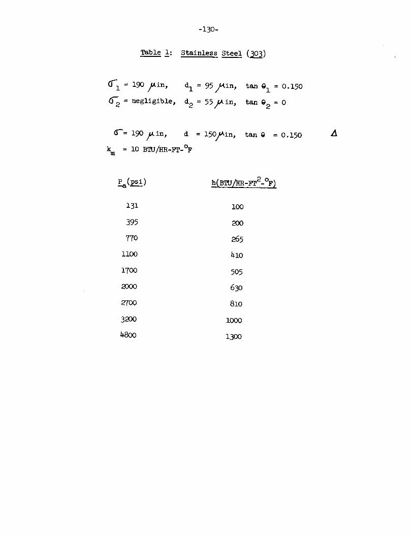
-13o-
Table i: Stainless Steel (303)
_-i = 190 /_in,
_= negligible,
dI = 95/_in,
d2 = 55/LAin,
tan @I = 0.150
tan @2 = 0
_": 190 _in, d = 150_Ain, tan @ = 0.150
P(psi)
131
395
77O
ii00
17OO
2OOO
2700
32OO
lO0
2OO
265
41o
505
63o
81o
1000
13oo
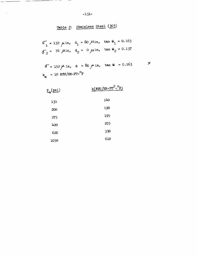
-131-
Table 2: Stainless Stee_____!l(30__3)
6"-2= 76 /Ain, d2 = O,/_in,
tan @i = 0.163
tan @2 = 0.137
d'-= 152_in, d = 80_in,
k = lO BTU/HR -_T-°Fm
tan @ = 0.163
_Cp____.)
131
275
620
lO5O
h(BTU/_-_2-°F}
14o
19o
195
e55
3_
61o
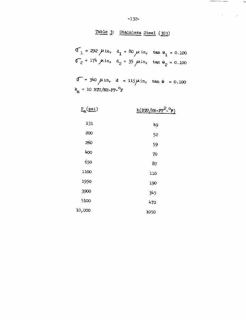
-132-
Table 3: Stainless Steel (303)
tan @i = 0. i00
tan @2 = 0.i00
d--=340/_in,d = ll5_in,
km : lOB_/_-_-°F
tan @ = 0.I00
131
2oo
_oo
4oo
65o
ii00
195o
39oo
5100
i0,000
49
52
59
7O
87
llO
190
345
47O
i050
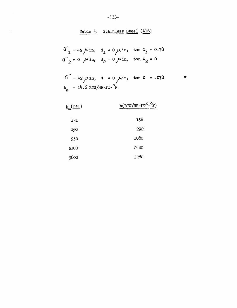
-133-
Table 4: Stainless Steel (416)
tan @i = 0.78
tan @2 = 0
= 42/_Ain, d = O/_in,
k = 14.6 B_J/HR-_T-°Fm
tan @ = .078 0
P_a(Psi )
131
190
95o
2100
38OO
h(B /HR-n2-°F)
158
292
1080
2480
328O
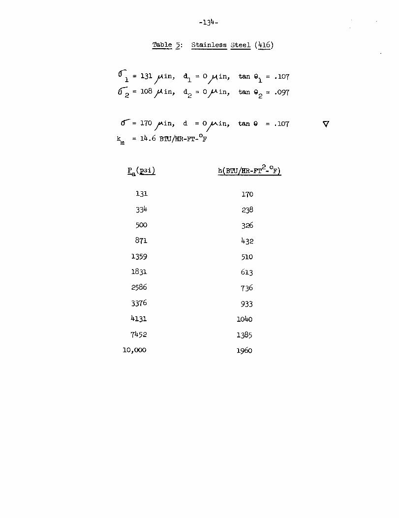
Table 5:
-134-
Stainless Steel (416)
i = 131/in,
_2 = 108 _Ain,
= O/_in, tan @l = .107
d2 = O/4Ain, tan @2 = .097
d" = 170/_in, d = O/_in,
k : 14.6 B%I//HR-_T-°Fm
tan @ = •107
131
334
5OO
871
1359
1831
2586
3376
4131
7452
i0,000
170
238
326
432
510
613
736
933
lO4O
1385
196o
V
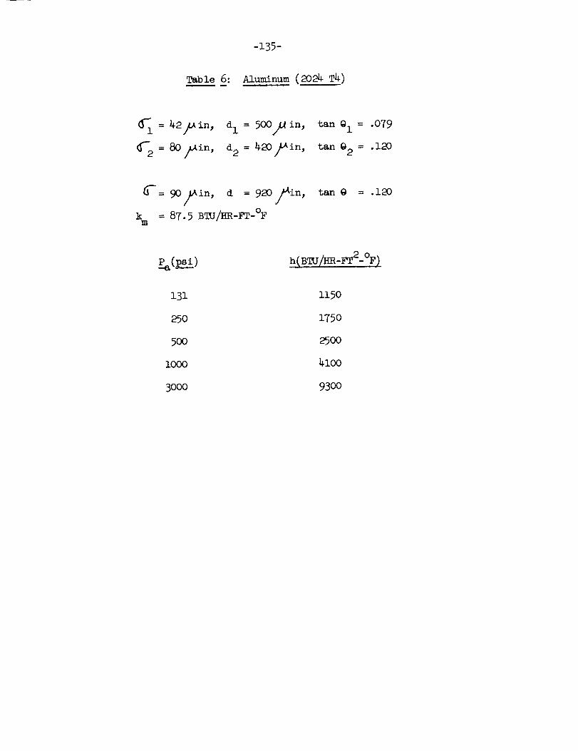
-135-
Table 6: Aluminum (2024 T4)
d I = 500/_ in,
d 2 = 420_in,
tan @i = .079
tan @2 = .120
_-= 90_in, d = 920_in,
k = 87.5 B_J/HR -FT-°Fm
tan @ = .120
h(B_J/HR-FT2- °F)
131
25O
5OO
lOOO
3ooo
i150
175o
25oo
41oo
93OO
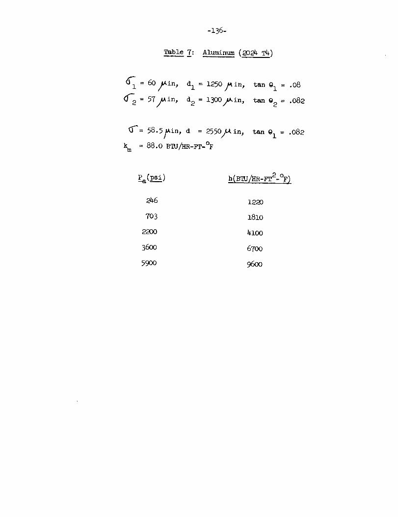
-136-
Table 7: Aluminum (2024 T4)
_i : 60/Ain, dI : 1250_in,
= 57/_in, d 2 = 1300_in,
tan @i = .08
tan @2 = .082
_'_= 58.5#in, d = 2550/L& in,
k = 88.0 BEI3/HR-FT-°Fm
tan @i = .082
h (BTU/HR-FT2-°F)
246
703
220O
36oo
59OO
1220
1810
4100
6700
960o
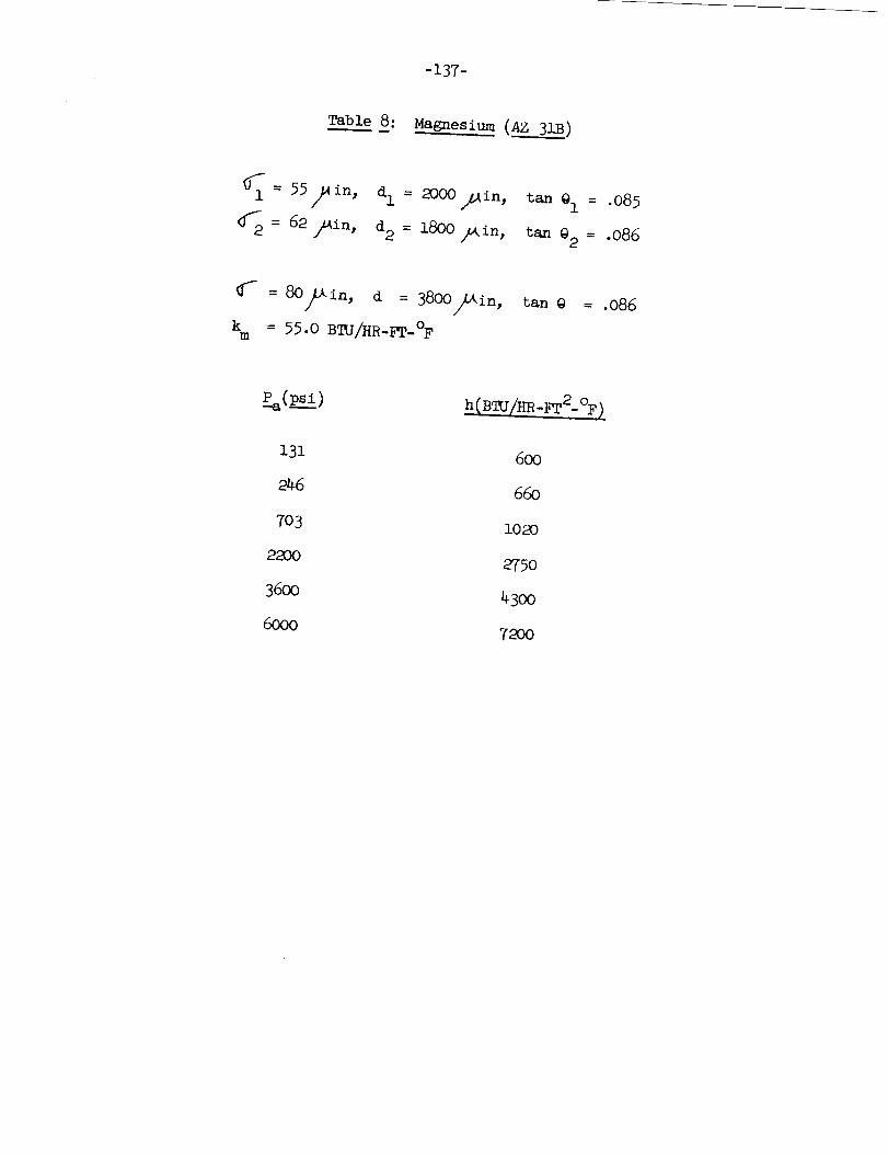
-137-
Table 8: Magnesium (A_Z 31B)
= 55/_ in,
G = 62/_in,
dI = 2000///in,
d2 = 1800 2u_in,
tan @l = .085
tan @2 = .086
_- : 80/_in,d : 3800/_in,
k = 55.0 BTU/HR-_T_°Fm
tan @ = .086
_(psi)
131
m6
703
22O0
3600
6000
6oo
660
lO2O
2750
43OO
72O0

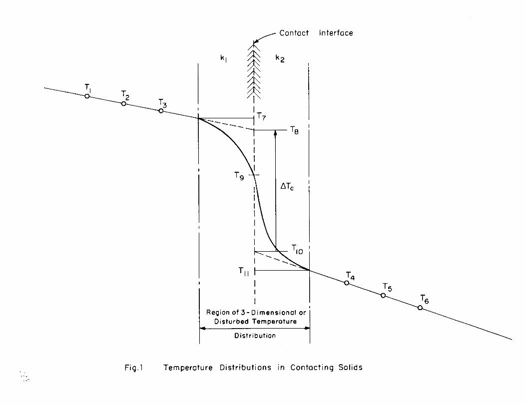
TI
k I
/ Contactj,,
/ \
_ k2
\
\t"\\\
T7
T8II
Interface
T 9
I _TcIIIIII
I
Region of 3- D
Disturbed
imensionol o=I
Temperoture
Distribution
7 5
Fig.1 Temperature Distributions in Contacting Solids
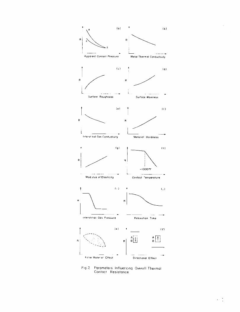
c_ (a]
b
Apparent Contact Pressure
(b)
Metal Thermal Conductivity
(c)
Surface Roughness Surface Waviness
(d)
le,T
Material HardnessInterstitial Gas Conductivity
(f)
Modulus of Elasticity
(g) ,_
~ 1000 °F
Contact Temperature
(h)
irlterstlha_ Gas Pressure
(i) (j)
Relaxation Time
T (k) ], C >'_, AmR \- R _ B L_
L[ . _
Filler Material Effect Direchonal Effect
(t)
B
F_g.2 Parameters Influencing Overall Thermal
Contact Resistance
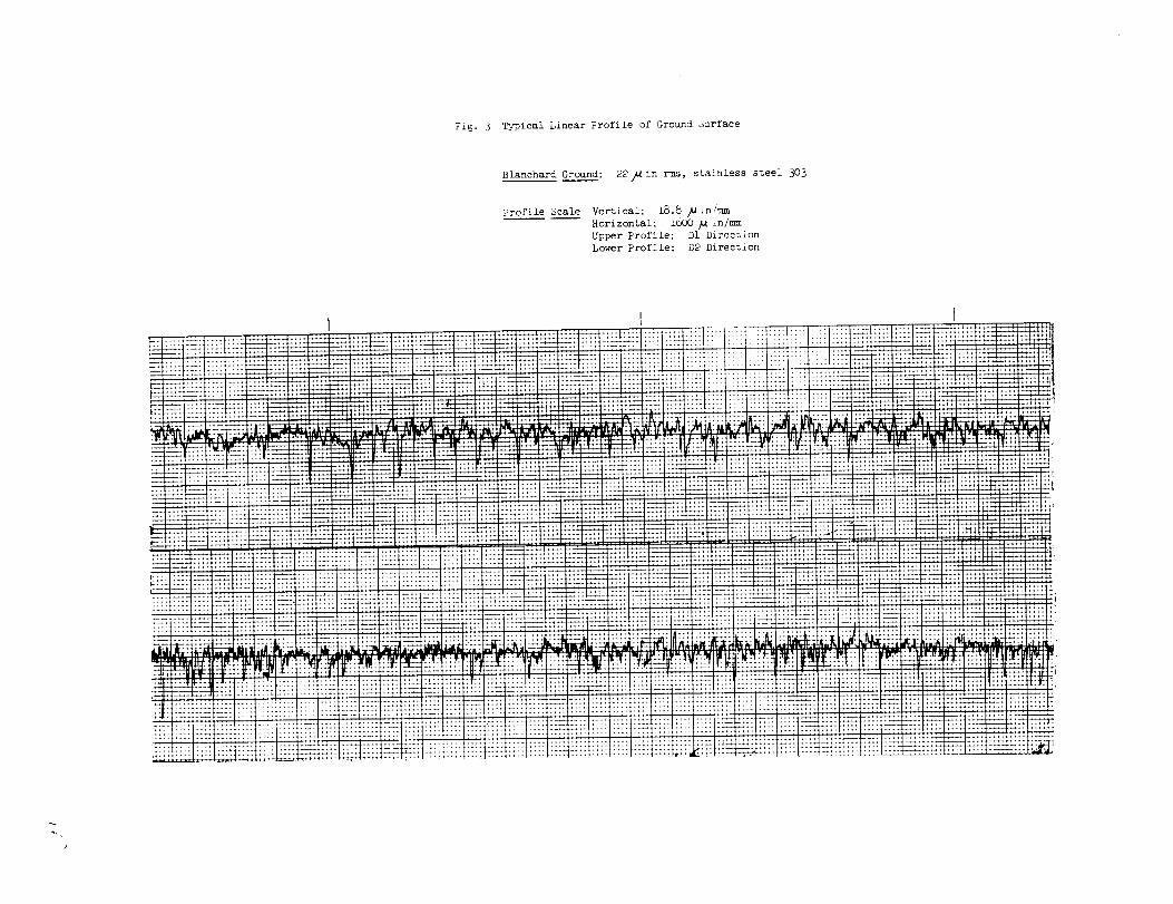
Fig. 3 '_ypical Linear Profile of Ground Surface
Blanchard Ground: 22]_in rms, stainless steel 303
Profile Scale Vertical: 18.8 _inlmm
Horizontal: iOOO jutin/ram
Upper Profile: D1 Direction
Lower Profile: D2 Direction
I I
[ .... :=::::_=::_2!ii:::'i :::::: _:!_:iii_! _ _.i
: ::::::::::::::::::: : I: ',!_ _I_ !:: ....... ,:_ _ _: ......
:_!iil!_: :_:2:_i_:ii!i i:.77.... :::: :::" :::: :::: ........ =:: :::: ..... "........ ::= =:: ::= :::: .......
,i.
z
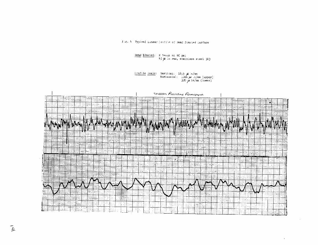
_'ig. & ?ypical Linear i:roliie of Bead Blasted Surface
Bead Blasted: H Beads at _0 psi
45_ in rms, stainless steel 303
P:'ofile Scale: Vertical: 18.8 _ _n/mz
Horizontal: i60b/u [n/mm (upper)
3_3/_in/mm (lower)
IL_ :::
---: ::l
it 2:_. ::
ii :i
7: i!L/ ..
l:ii L
L
'- Z
2_2 12 ="
2
::i ::
i!i 77
&
-i :i Z: ......::: :2: "_ :r: ::7 _ :2:
+_ ._ :: _ ::2 _
_: '_ _: 7: ::/ * -_
72 :: "- ....
T- -- .. :7 gTJ ....
:7 ii _I'- 72"
=."-: i[ =:........ : i!
[ .1
t_: :q :: n
-2 i: ii !! _i.
22 :i :': :12
.: L_
=: ::_
[21 2=
• i
7:
2: _.2
÷- r"
= =
:: t]?:1
:2 ::2
21 :'2
i] :2i
:: ii2.* ..
21 ::
22 :.
:: !!
:_L_::_:-:::=:::7:_:77::::::::::::,:::: Iili,_,,,:,_::£J: ; :
: : :2
:: 2_.
,.f.f
12 =2-
2:: :2
":_ 172
÷.
:2-
27 "1
:± l±
L._ 2.
',:: ::
::: ::
:L: 77
::: ::
__
:: 72
ii "
i: i2
!!i i.::: 11
i! ii, J
"_ii
ii i
!!:
::i:"
i.i i!.
2--
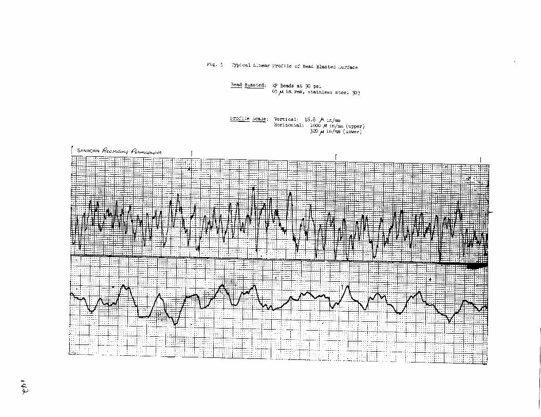
Fig. 5 Typical Linear Profile of Bead Blasted Ourface
Bead B±asted: XP Beads at 90 psi
65/Ai_ r ms, stainless steel 30 3
Profile Scale: Vertical: 18.8 /A in/rmm
Horizontal: 16OO_ in/mm (upper)
32024in/= (lower)
:'.: :;:
:::: i: i::ii:_L!i!ii;i
,,i "'!'
",l:JJ-i!l!l'ltriilii;il[
N!i ":..'_
_._
.... ÷__.
.... + ....
i
....T-:;÷
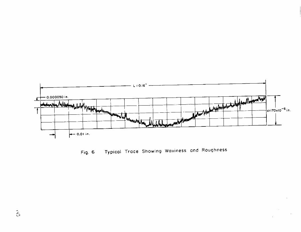
0.000050 in
.-_ _-- 0.01 in.
• l
II
L - V,iv
IAl
I , _._,_£-
l
-6.d:17OxlO in.
Fig. (5 Typical Trace Showing Waviness and Roughness
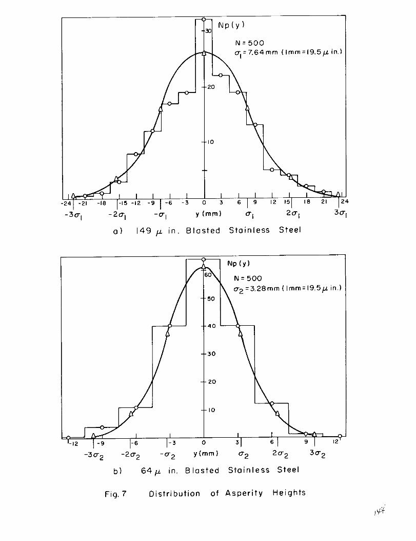
I I
-24 -21 -18 1-15-12 -9 I-6-30- I - 2o- I -o- I
I I
a) 149 /.L in.
,_Np(y )N : 500
0-1= 7,64 mm( Irnm : 19,5/_ in.)
\
-20
I0
I I-3 0 3
y (ram)
I I I6 I 9 12 15 18 21 24
0-1 2°'1 :5°'1
Blasted Stainless Steel
_j-30- 2 -20- 2
b)
---%
/ Np (y)N= 500
0-2 =3.28 rnm (Imm=19.5_ in.)'50
.40
-3O
I
t-2o
64/.z in.
-_-I0
i
y (ram) 0"2
Blasted
20- 2
Stainless Steel
Fig, 7 Distribution of Asperity Heights
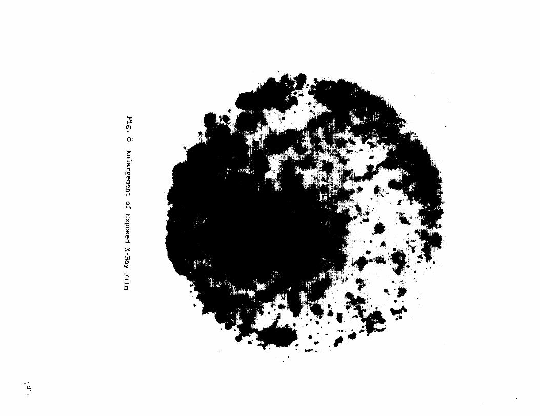
o_i
Co
O_
c+
0
o
!
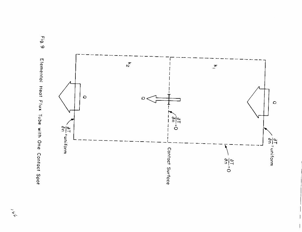
7"I--.
rrl
11)3
I"7
7-I'D0
77
I'-X
l-l:Jr11)
IEm_
0
C)0
0¢)
(./)
0
0
3
I
I ii
I 0III
c_i")
(./)r-
"-h
0¢)¢D
II
0
c)
\II
o-
_h
0
3
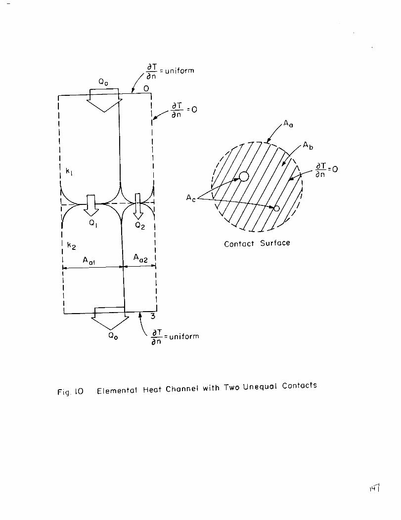
Qo
aT= uniform
/0 On
II OT
i1_-g _- =o
I kI t
_ Q2 I
I i
I k2 II I
I Aol Ao2 I
I II II II It J
Qo OT =uniforman
/
Ac Z
Ao
-', i /\ aT
Contact Surface
Fig. I0 Elemental Heat Channel with Two Unequal Contacts
,4
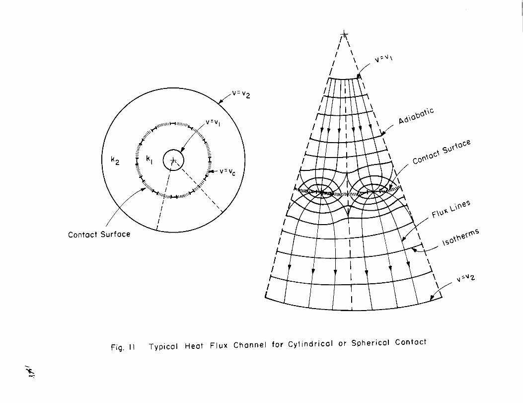
v 2
/k2 k I
_,,,,. / ".,,,-_- /
Contact Surface/
I/
/
/
/
/ \/ \ _¢'g\
/ \
\
\
Fig. 1] Typical Heat Flux Chonnel for Cylindricol or Spherical Contact
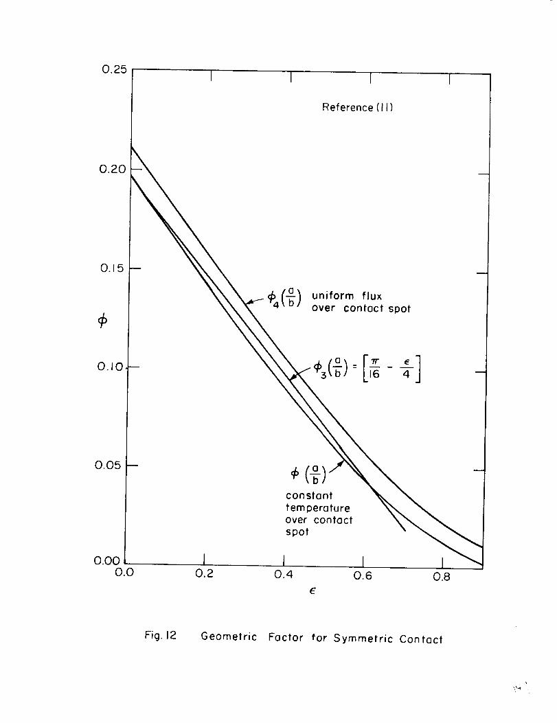
0.25I I I I
Reference (11)
0.20
0.15
"6- uniform fluxover contact spot
0. I0
0.05
constant
temperature
over contactspot
0.00 I I I 10.0 0.2 0.4 0.6 0.8
Fig. 12 Geometric Factor tar Symmetric Contact
\_.J, ,
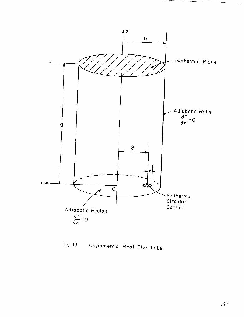
g
Adiabatic RegionaT
_=0az
--- Isothermal Plane
Adiabatic WallsaT
_=0ar
Isothermo_Circular
Contact
Fig. 13 Asymmetric Heat Flux Tube
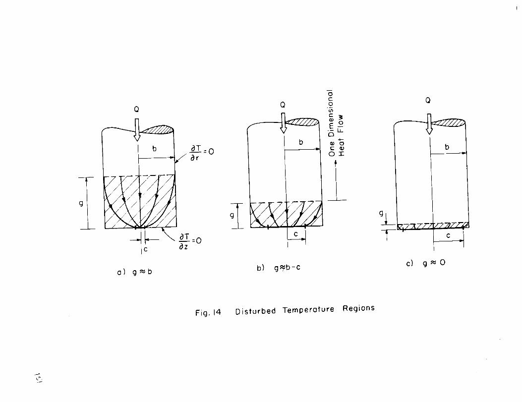
Q
a) g_,b
Q
(3c-O
_oEIT
b _ o
ol-
bl g_/b-c
Q
I "
b
C
c) g_O
Fig. 14 Disturbed Temperature Regions
L"

\
\
\
\
\
\
\
\
\
\
\
\
\
\
\
\ L
,\\\\\_Lc
I-
b
I\\l I
\ \
\ \
\ \
\ Isothermal \\
Surface \\\
\ \\ \N \N \\ \\ \\\ \ !
Fig. 15 Asymmetric Constriction Resistance Model
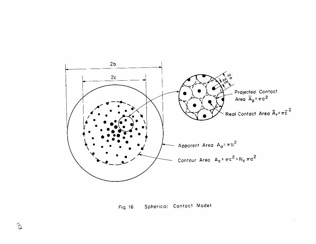
2b
2c O
Apparent Area
Contour Area
Projected Contact
Area Ap = Tra2
_2Real Contact Area Ar='n'c
Ao = Trb 2
A c : .n-c2 = N c 77-o2
Fig. 16 Spherical Contact Model
J
VkL4
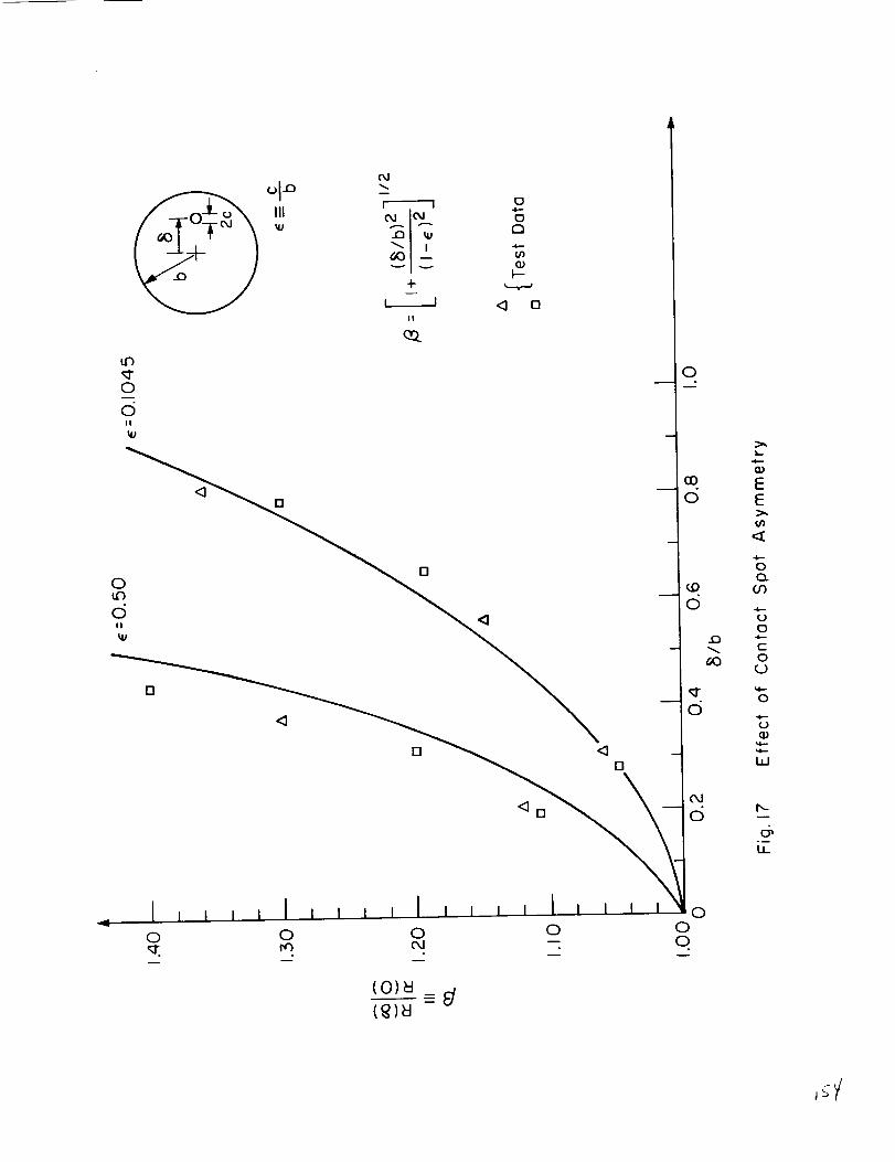
_ro
dII
_1_III
4-
L_JII
o
oQ
,4,--
(/1Q)
t--
[] _ _0
_ Illlllll,,lll,,l'll'o 0 0 o
0
03
0
_O
0
6O
,<r
c5
OJ
d
0
(0)_ -J
EE
0o.
,4--
uI3
co
(J
o
,4---
tj
I,I
d,°-
lJ--
IIri
//
//
//I
\\\\
\\
\
ff
f
\\
\\\\
II/
//
//
//
/
............ ....I Boundary of
Apparent Area
Fig. 18 Displacement Region for Nominal Asymmetry Effect
15b
6
m
7 =
0
7"1
CX
C
0c
o.o
0
3121
0
Q
U)"U0
O0
BrassElectricalConnection
CopperElectrode
iIIIIIIII
II
11
5 mil
Plexiglas Tubes
iI II II I
II II II II I
I II II 1
Mylar Sheet
IIIIIIII
I
II
Fig. 20 Liquid Analog Apparatus to Test for Asymmetry
JVk
5mil. Mylar Sheet
Plexiglos TubeL/2
Distilled Water with
Few Groins of Salt
L = 16.31 in.
D = 5.46 in. CopperElectrode
Fig. 21 Liquid Analog Apparatus to Test Variable Size Effect
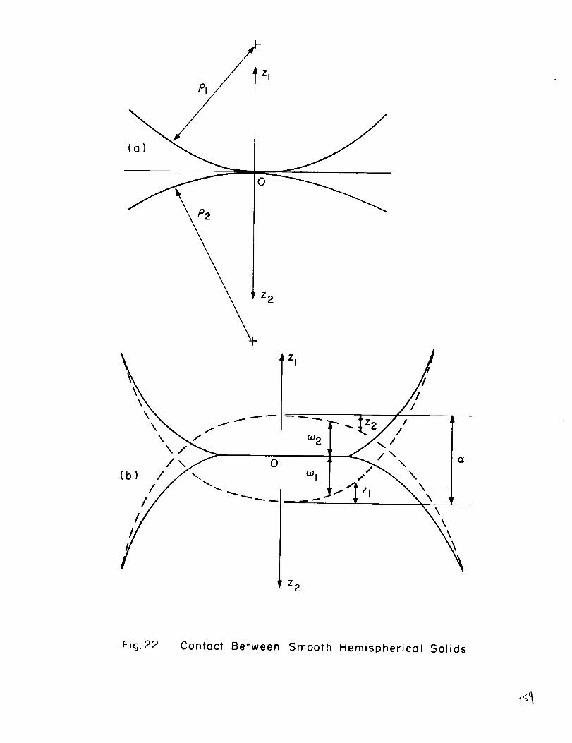
.q-
PI/ zl
z I
7
i I
\/
o
2 2
Fig. 22 Contoct Between Smooth Hemispherical Solids
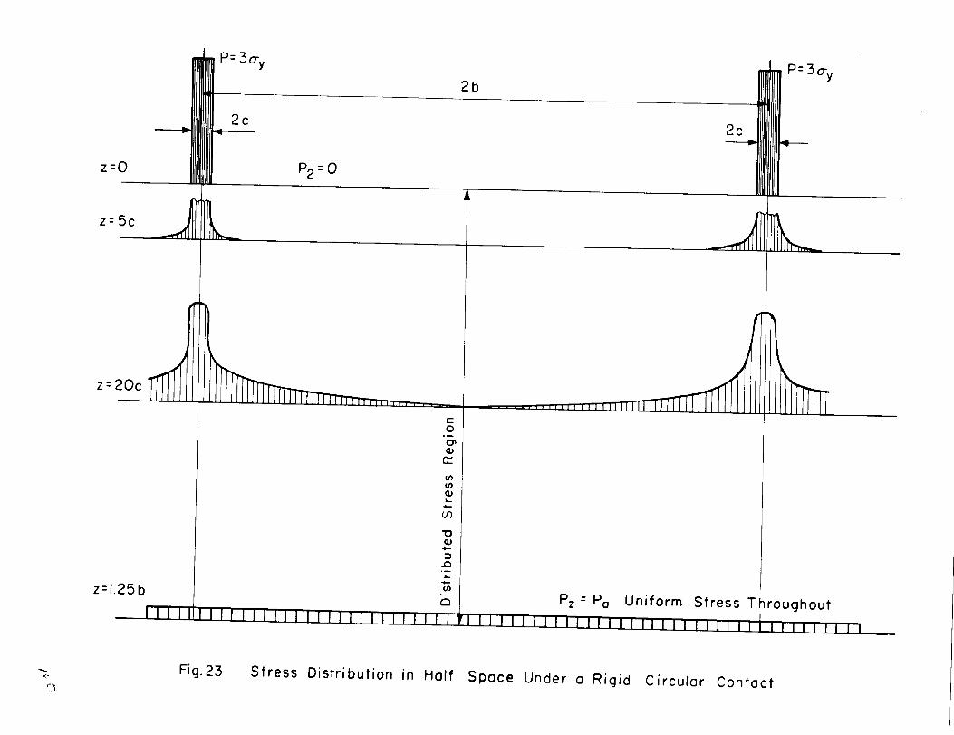
P= 3O'y
2c
2b
2c
P= 3O'y
z=O P2= O
Z:SC
20Cz:
z=l.25b
t-O
cr
u3
¢.,,
°__
Q Pz = Po Uniform Stress Throughout
Fig. 23Stress Distribution in Holt Spoce Under o Rigid Circulor Contoct
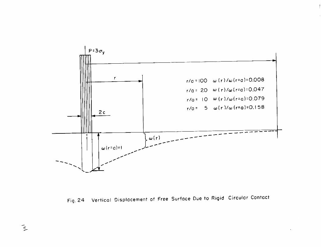
P=3o'y
(_(r=a)=l
rio =I00
rio = 20
r/a = I0
r/a = 5
(r)/_(r=a)=O.O08
( r)/_(r=a):O.047
(r)/_j(r=a):O.079
(_(r)/_ (r=a)=O.158
_ _ m _ _ _ __
Fig. 24 Vertical Displacement of Free Surface Due to Rigid Circular Contact
f
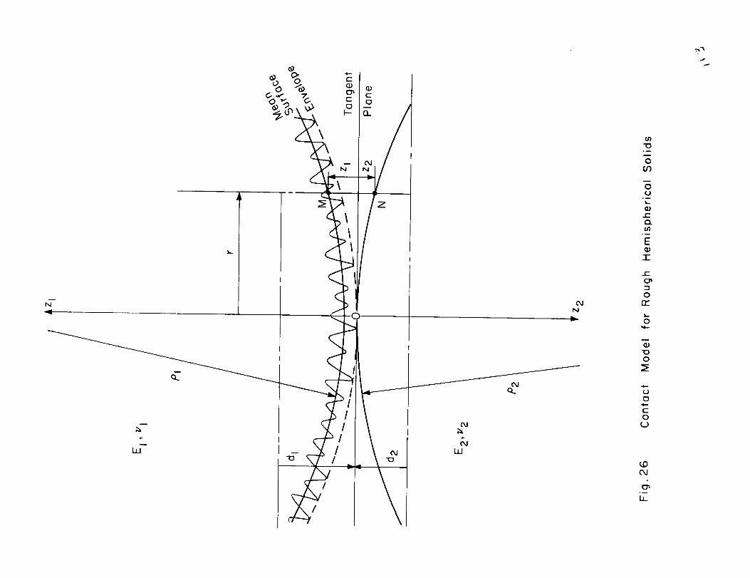
0
m
N
I
CL
WAJ
W
(xJN
007oo_
0O0
m
ou°D
o.
E
"I-
0rr
o
o
o
Eo(J
_0
b_
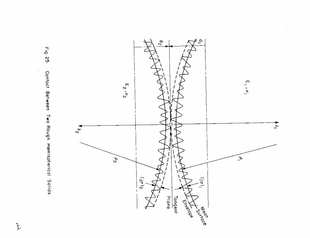
"rl--.
00
Q
CO
¢D
"-'1
-I
0
0
.-r_D
3
m°
O
CO0
0
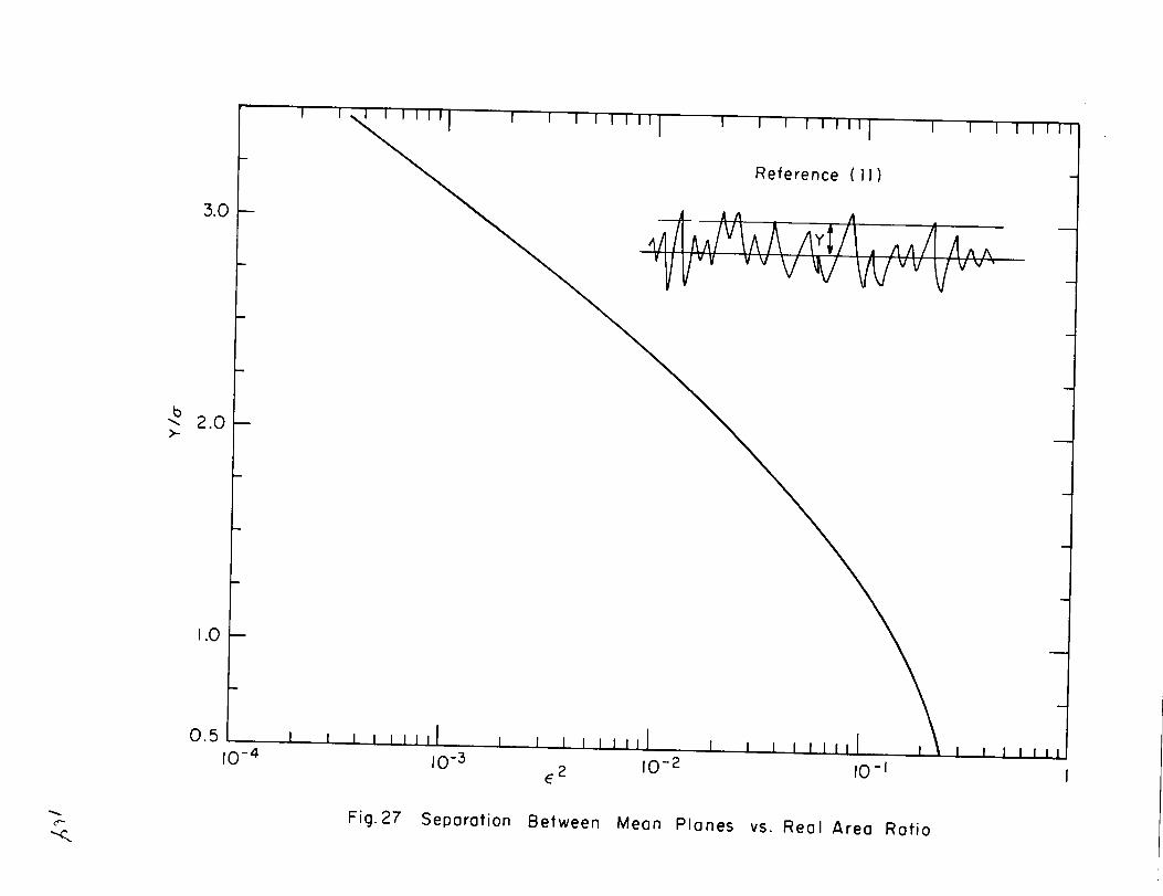
3.0--
b"_ 2.0-->,-
1.0 --
0.5
10-4
1_, I I II I r i i i i i ii I t i i i i lil I I I I
Reference (ll)
v',5
IO-3 2 lO-2 tO -t
I I 11
I I ill
Fig. 27 Separation Between Mean Planes vs. Real Area Ratio
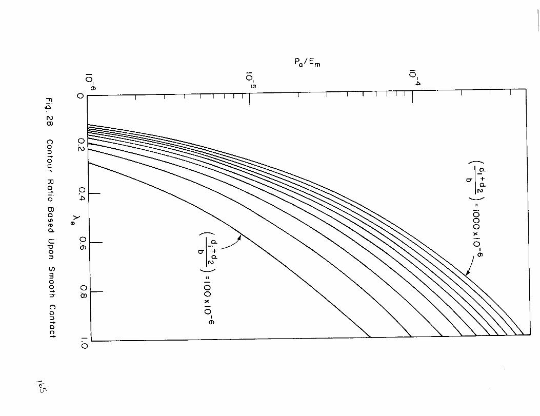
77
GO
0
0f-
0
0
0
O.
C'100
300
0
0
0"-L_
0
0
0
000
I 1 I I I
m
O,
PolEm
I I I I I
m
0I
11
000
0I
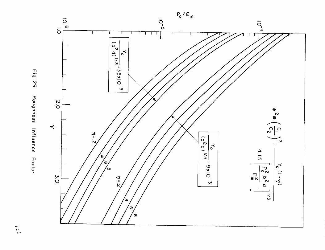
"1"I_o
uo
rO_D
::0Oc-
_oo_o_
m
r-
(-)
-qo
o
8,
fO
b
b
I i i I
I!
O0X
C>!
b_
i!
I!
C)!
i I I i I
i
Po/Em
II
_0
CDIoJ
m
O!
HI
roII
I •
%r_
i j
0
N-
v
_0
r_TM
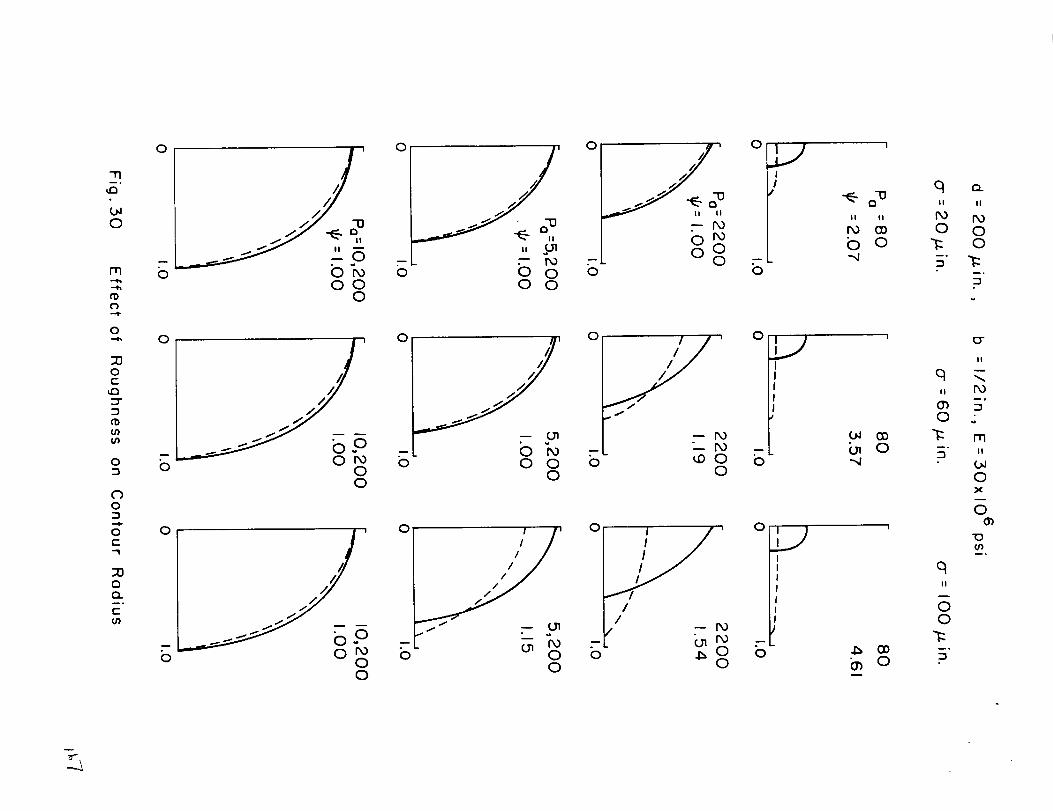
-tl_°
,rm
0
m
¢D
o
or-
_r
¢DcJ)
0
0
oI #iOl/oZ -D _ '
-1 -____.__ "_ L o_ .-b '--"'-- b_ o o oO0 0 o
0
°.LII
t-O
, 01 @,, 0 0 I
o OnO o 0 0 o i.oO o0 0 00
,-I,,
0
"1
;130O._°
i-
II II
PO (3O
b o",4
_ 0"-4
q e'_
II II
PO PO
0 0"_ 0
5" "I_
II
qii IX)
_o
0
0X
0
_°
qII
00
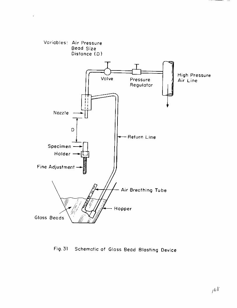
Variables: Air Pressure
Bead Size
Distance (D)
IIII
Nozzle
Va I ve Pressure
Regulator
Glass
Hopper
Return Line
Air Breathing Tube
High PressureAir Line
Fig. 3l Schematic of Glass Bead Blasting Device
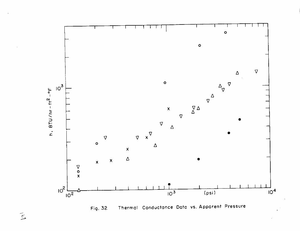
u_ 10 3o
I
I
f-
F--
m
102
m
m
VO
X
10 2
O
X
I I I I I I I I I I 1 II
O
o
X
VA
O
A
V
VAA
V
V V x
X
XA
A
I I I I I I I I I I I
10 3 (psi)
I I I
V
I I I I
m
104
Cr
Fig. 32 Thermal Conductance Data vs. Apparent Pressure

0.4,--
_c
b
I0 -I
-2I0
10-3
B
f I I I I I I I
10 .4
I0 -4
• X _7
I I I I II I'1 I I I I I I I II
m
m
m
, I , I ,,_ll t I I _ ,,ill , j , , ,,,,
10-3 e2 I0 -2 IO -I
Fig :5:5 Thermal Conductance Number vs. Area Ratio
t 7C_
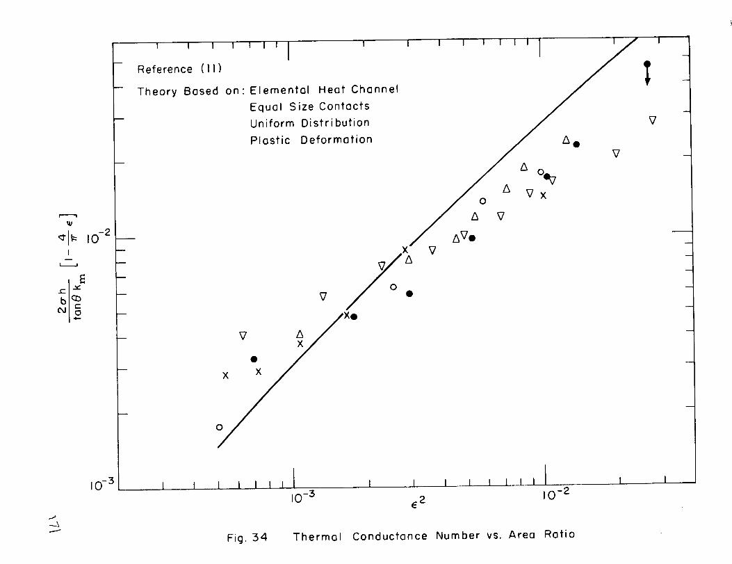
I
_u
_rl:= iO -2I
b
10 -3
-- Reference (il)
-- Theory Based on' Elemental Heat Channel
Equal Size Contacts
-- Uniform Distribution
Plastic Deformation / A e%7/
AVe- x _7
-- V •
- V _/xo
III i i i i I II I i i i , i , ii
IO -5 2 IO-2E
Fig. 34 Thermal Conductance Number vs. Area Ratio
i
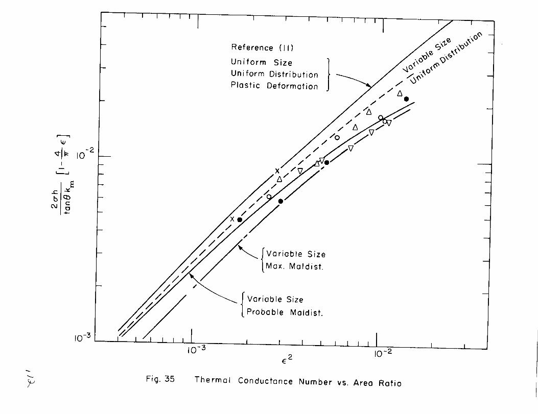
I i I i
Reference (11)
Uniform Size ]Uniform Distribution
Plastic Deformation
//
/X s
I I I I j
Variable SizeMax. Maldist.
Variable SizeProbable Moldist.
Fig. 35
I I I I I I I I I
I0 -3 10-22
E
Thermal Conductance Number vs. Area Ratio
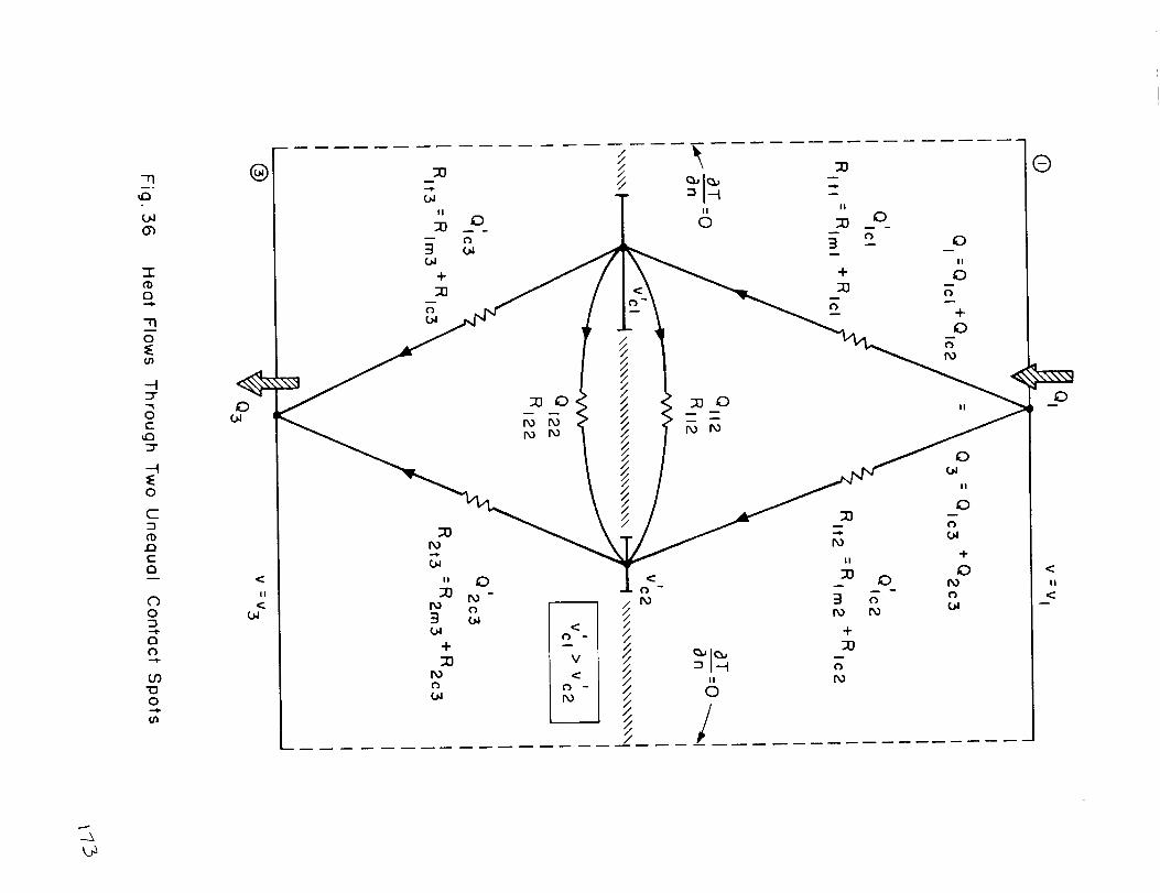
77
(JJO_
7"¢1)0
"11
0:E
.-q
0c
_c_
-q_Eo
C-7(1).Q(-c}
C)o
m o.
0c)
Ch"o0
fit}
J
®
II
o
®
I!
--1
L_
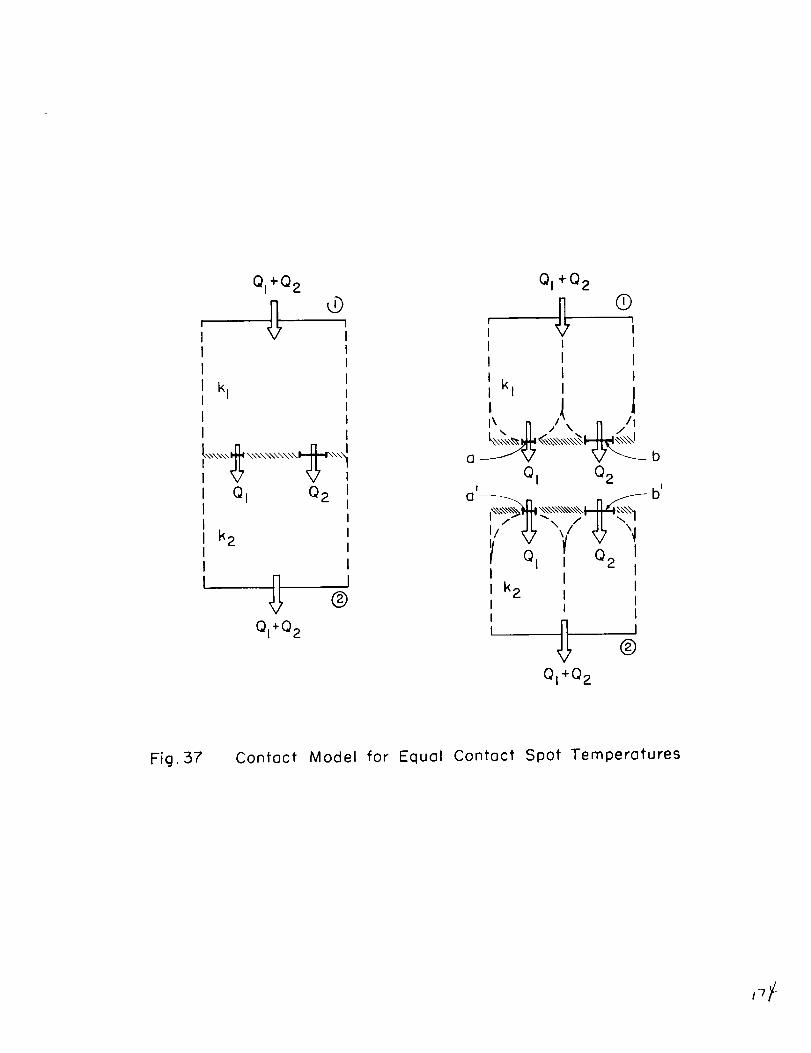
QH+Q2
o1 iI II I
I i
I k I II III II i
I V V i
I QIIII k2III
Q2 IIIIIIJ®
QI+Q2
Q +Q2
(:!:)
l lt li I
QI Q2a' b'
n /fll"\ /" II \i
t QI I Q2I II k 2 II II
' _ ®QI+Q2
Fig.37 Contact Model for Equal Contact Spot Temperatures
#v/¢