Infinite labeled trees: From rational to Sturmian trees

Theoretical Computer Science 411 (2010) 1146–1166

Contents lists available at ScienceDirect

Theoretical Computer Science

journal homepage: www.elsevier.com/locate/tcs

Infinite labeled trees: From rational to Sturmian treesNicolas Gast a,b,∗, Bruno Gaujal a,ca Laboratoire Informatique de Grenoble, UMR 5217, 110 av. de la Chimie, 38041 Grenoble, Franceb Grenoble Universités, 38041 Grenoble, Francec INRIA Grenoble - Rhône-Alpes, 655 avenue de l’Europe, 38 334 Saint Ismier Cedex, France

a r t i c l e i n f o

Article history:Received 22 April 2009Received in revised form 2 October 2009Accepted 13 December 2009Communicated by M. Crochemore

Keywords:Infinite treesSturmian wordsSturmian trees

a b s t r a c t

This paper studies infinite unordered d-ary treeswith nodes labeled by {0, 1}.We introducethe notions of rational and Sturmian trees along with the definitions of (strongly) balancedtrees and mechanical trees, and study the relations among them.In particular,we show that (strongly) balanced trees exist and coincidewithmechanical

trees in the irrational case, providing an effective construction. Such trees also have aminimal factor complexity, hence are Sturmian. We also give several examples illustratingthe inclusion relations between these classes of trees.

© 2009 Elsevier B.V. All rights reserved.

1. Introduction

Let us consider the following question: how to distribute ones and zeros over an infinite sequencew = (wn)n∈N such thatthe ones (and the zeros) are spread as evenly as possible. In a more formal way, the sequence w is balanced if the numberof ones in a factor wi, . . . , wi+`−1 of length `, does not vary by more than 1, for all i and all `. Such sequences exist and arecalled Sturmian wordswhen they are not periodic.Sturmian words are quite fascinating binary sequences: they have many different characterizations formulated in terms

coming from as many mathematical frameworks, in which they always prove very useful. For example, Sturmian wordshave a geometric description as digitalized straight lines and as such have been used in computer visualization (see [15] fora review). They can also be defined with an arithmetic characterization using a repetitive rotation on a torus or continuedfraction decompositions. From a combinatorial point of view, yet another characterization of Sturmianwords is based on thebalance between ones and zeros in all factors, as mentioned before. They are also used in symbolic dynamic system theorybecause they are aperiodic words with minimal factor complexity or because they have palindromic properties. Most ofthese equivalences have been known since the seminal work in [18]. More recently, Sturmian sequences have also beenused for optimization purposes: they are extreme points of multimodular functions [14,2,13] and this has applications inscheduling theory [12].Since then, there have been several constructions of generalized Sturmian words in the literature.The first one concerns words over more than two letters. Billiard sequences in hypercubes extend the torus definition

of Sturmian sequences while episturmian sequences [3] extend the palindromic characterization of Sturmian words,however, the other characterizations of Sturmian words are lost in both cases. Another extension is to two dimensions.A complete characterization of two-dimensional non-periodic sequences with minimal complexity is given in [7], hereagain the alternative characterizations are lost. Yet another extension of Sturmian words concerns discrete planes. Indeed,

∗ Corresponding author at: Laboratoire Informatique de Grenoble, UMR 5217, 110 av. de la Chimie, 38041 Grenoble, France. Tel.: +33 476612031; fax:+33 476612099.E-mail addresses: [email protected] (N. Gast), [email protected] (B. Gaujal).

0304-3975/$ – see front matter© 2009 Elsevier B.V. All rights reserved.doi:10.1016/j.tcs.2009.12.009

http://www.elsevier.com/locate/tcs

http://www.elsevier.com/locate/tcs

mailto:[email protected]

mailto:[email protected]

http://dx.doi.org/10.1016/j.tcs.2009.12.009

N. Gast, B. Gaujal / Theoretical Computer Science 411 (2010) 1146–1166 1147

several characterizations of Sturmian lines can be extended to discrete planes. There exist interesting relations betweenmultidimensional continued fraction decomposition of the normal direction of an hyperplane and the patterns of itsdiscretization. These relations mimic what happens for Sturmian sequences, [10]. Finally, another generalization is toordered trees [4], where Sturmian trees are defined as infinite binary automata such that the number of factors (subtrees)of size n is n+ 1. The other characterizations of Sturmian words are lost once more.The aim of this paper is to do the same for unordered trees where things work better in the sense that several extensions

coincide. We introduced in [11] a new type of infinite tree: unordered labeled trees, for which the left and right children ofeach node are not distinguishable and gave a brief presentation of their main properties. Here, wemake an exhaustive studyof such trees. We show that the balance property (even distribution of the labels over the vertices of the tree) coincides witha characterization of trees using integer parts of affine functions (called mechanicity). Furthermore these strongly balancedtrees have a minimal factor complexity. Therefore, they can be seen as a natural extensions of Sturmian sequences in morethan one aspect. This brings some hope to use them as extreme points for adapted optimization problems.Our purpose in the paper is two-fold. The first part of the paper is dedicated to the study of general unordered infinite

treeswith binary labels. In Section 2,we provide definitions of themain concepts aswell as the basic properties of unorderedtrees with a special focus on the notion of density (the average number of ones) and rationality. Section 3 is dedicated to thestudy of the rational trees.The second part of the paper investigates balanced unordered trees and their properties. In particular, we show that

strongly balanced trees (defined in Section 4) are mechanical (so that they have a density and all labels can be constructedin almost constant time). Furthermore their factor complexity is minimal among all non-periodic trees. We also investigatethe general shape of strongly balanced rational trees (Section 5). We show that there essentially exists a unique stronglybalanced tree with a given rational density. Also, once a strongly balanced tree is given, its density is easy to compute andwe provide an efficient algorithm with polynomial complexity to test whether a rational tree is strongly balanced. Finally,Section 6 presents several examples and counter examples that illustrate the different notions presented in the paper.

2. Infinite trees

2.1. Ordered infinite trees or tree-automata

Ordered infinite trees (also called tree-automata here) have been studied in [8,4]. Ordered infinite trees are automata withan infinite number of states. An automaton is a tree-automaton if it has one initial state and each state has a uniform in-degree equal to one (except for the initial state, whose in-degree is 0) and a uniform out-degree dwith labels a1, . . . , ad onthe arcs. Every node v is labeled by `(v) = 1 (resp. 0) if it is final (resp. non-final).The language accepted by the tree-automaton T is a subset ofA∗ (where the alphabetA = {a1, . . . ad}) and is denoted

byL(T ). Thus, a wordw in the free monoidA∗ corresponds to a node in T , and a wordw inL(T ) corresponds to a node inT with label 1. Conversely, a unique tree-automaton can be associated to any subset L ofA∗, by labeling by one the nodescorresponding to the words in L.Classically for automata, a family of equivalence relations can be defined over the nodes of tree T : v ∼0 u if `(v) = `(u),

v ∼n+1 u if v ∼n u and for all i, the ith child of u, uai and the ith child of v, vai satisfy uai ∼n vai. By definition of∼n, u ∼n vif and only if the subtree rooted in u of height n is the same as the subtree rooted in v of height n.

L(T ) is recognized by its minimal deterministic automaton (possibly infinite), say A(T ). Actually, A(T ) can be obtainedfrom the tree T by merging all the states in the tree in the same equivalence class of∼n for all n.An example is given in Fig. 1 where the infinite tree-automaton and the minimal automaton recognizing all the prefixes

of the Fibonacci1 word over the alphabet {a, b} is given together with the corresponding minimal automaton (which has aninfinite number of states).The number of distinct subtrees of height n in T is called the complexity P(n), of T . P(n) is the number of equivalence

classes of∼n. If P(k) ≤ k for at least one k, then it can be shown [4] that the complexity P(n) is bounded by k. This impliesthat theminimal automaton A(T ) has less than k states. The tree is therefore rational, since it recognizes a rational language.If a tree-automaton T is such that P(n) = n + 1 for all n, then it has a minimal complexity among all non-rational

trees. Such trees have been shown to exist and are called Sturmian in [4] by analogy with the factor complexity definitionof Sturmian words (Fig. 1 gives an example). In [4] several classes of Sturmian tree-automata are presented. However suchtrees are not balanced and no constructive definition (as the mechanical construction for words) is known.

2.2. Unordered trees and minimal graph

In this paper, we rather consider a different type of tree, namely infinite directed graphswith labels 0 or 1 on nodes andwith uniform in-degree 1 and out-degree d ≥ 2. Up to our knowledge, these types of tree have not yet been considered inthe literature. The similarities as well as the discrepancies with ordered trees will be discussed all along the paper.

1 The Fibonacci word is the limit of the sequence fn+2 = fnfn+1 with f0 = a and f1 = b, see [16] for more details.

1148 N. Gast, B. Gaujal / Theoretical Computer Science 411 (2010) 1146–1166

Fig. 1. The tree-automaton recognizing the Fibonacci word f and the corresponding minimal automaton. The states of this latter are 0, 1 . . . ,∞. The finalnodes are filled in black. There is a transition between nodes i and i+1 labeled by the ith letter of f and one between nodes i and∞ labeled by the oppositeof this ith letter.

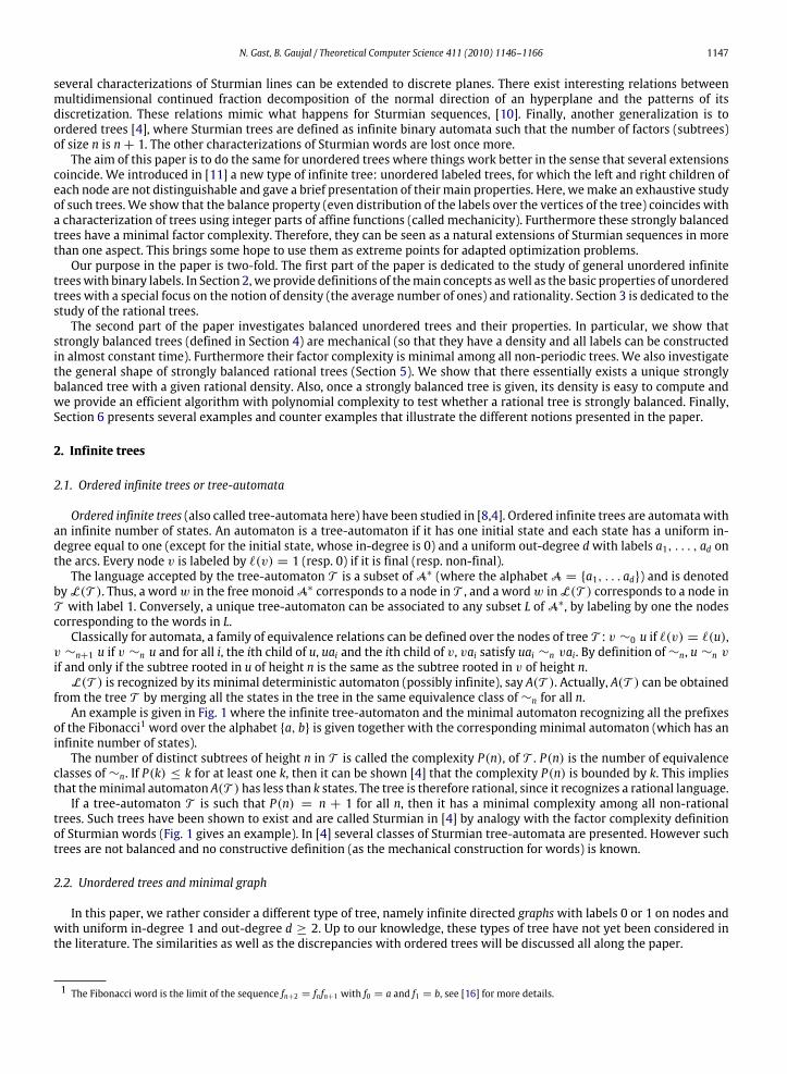
Fig. 2. A tree T and the associatedminimalmultigraph G(T ). The label of the black (white) nodes is 1 (0). The arcs are implicitly directed from top to bottom.

In such trees, one node is special (with in-degree 0) and is called the root. Also, the children of a node are not ordered.Thus, the main difference with the previous type of tree is the fact that arcs are not labeled. Therefore such trees cannot bebijectively associated with languages.We define the minimal multigraph (i.e.with multiple arcs) G(T ), associated with the tree T , mimicking the construction

of the minimal automaton for ordered trees. To do that, we first introduce a family of equivalence relations ≡n over thenodes of T :

• v ≡0 u if u and v have the same label: `(u) = `(v)• v ≡n+1 u if v ≡n u and if there exists a bijection F between the children of v and the children of u such that for all childw of v,w ≡n F(w).

Therefore, v ≡n u if and only if the subtree with root v of height n is isomorphic to the subtree with root u of height n. Bymerging the nodes of T when they belong to the same equivalence class of ≡n for all n, one gets the minimal multigraphG(T ) of the factors of T : all nodes merged in the same vertex of G(T ) are roots of the same subtrees, of every height. In G(T ),the node corresponding to the root of T is distinguished. (graphically, this is done by adding an arrow pointing to the node).An example of an unordered tree T is given in Fig. 2. Actually, most figures in this paper will represent binary trees

(with out-degree d = 2), although all the discussion is carried throughout for arbitrary degrees. The nodes of the associatedmultigraph G(T ) are numbered arbitrarily and nodes with label 1 are displayed with a bold circle. The node correspondingto the root of the tree is pointed by an arrow.There exists a way to associate an ordered tree-automaton T to a tree T by choosing an order on the children of each

node. This can be done by seeing G(T ) as an automaton by labeling arcs in G(T )with letters a1, . . . ad in an arbitrary fashion.Conversely, a tree-automaton T can be converted into a graph T by removing the labels on the arcs. This graph is called theunordered version of T . Fig. 2 is the unordered version of the tree recognizing the Fibonacci word displayed in Fig. 1. Notethat while the minimal automaton is infinite, the minimal graph G(T ) is finite, with only two nodes; one corresponds tothe subtree where all labels are 0 and the other one to the subtree with a branch with label 1 everywhere and all the othernodes with label 0 (Fig. 2).

2.3. Irreducibility and periodicity

By analogy with Markov chains, we say that a tree T is irreducible if G(T ) is strongly connected.


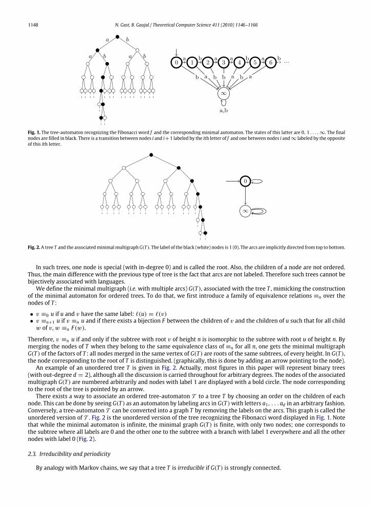
Fig. 3. Example of factors of a tree. On the left a factor of height 3 (and base 0) is surrounded in black. On the right is a factor of height 2 and base 2.

A non-irreducible tree, G(T ) is made of strongly connected components , inter-connected by an acyclic graph. Also, anirreducible tree T is periodicwith period p if the greatest common divisor of the lengths of all cycles in G(T ) is p. A tree withperiod 1 is also called aperiodic.

2.4. Factors, complexity and Sturmian trees

In this paper, we will study the properties of factors of infinite trees. For this purpose, we introduce two definitions:

• A factor of height n (and base 0, by default) is a subgraph of T which is a complete subtree of height n. The number of nodesin a factor of height n is denoted by S(n) def= dn−1

d−1 .• A factor of height n and base k (with root v), is a subgraph of T which is the subtree of height k+ n rooted in v minus thesubtree of height k, rooted in v (see Fig. 3 for an illustration). Such a subgraph is also called a factor of shape (n, k) in thefollowing. The number of nodes in a factor of height n and base k is S(n, k) def= dn+k−dk

d−1 .

Similarly to what has been done for words or ordered trees, the factor complexity PT (n) of a tree T is the number ofdistinct factors of height n and base 0.The complexity of a tree PT (n) can be bounded by the total number of ways to label trees of height n and degree d, say

An. It should be clear that A1 = 2 (a node can be labeled 0 or 1) and that An+1 = 2M(An, d) whereM(x, y) is the number ofmultisets with y elements taken from a set with x elements. Therefore using binomial coefficients,

An+1 = 2(An + d− 1An − 1

).

This is a polynomial recurrence equation of degree d. A change of variable, un = log An + 1d−1 log

2d! yields a new recurrence

equation un+1 = (d+ εn)un where εn = o(1). This implies that An = φdn+o(dn) for some φ with 1 < φ < 2.

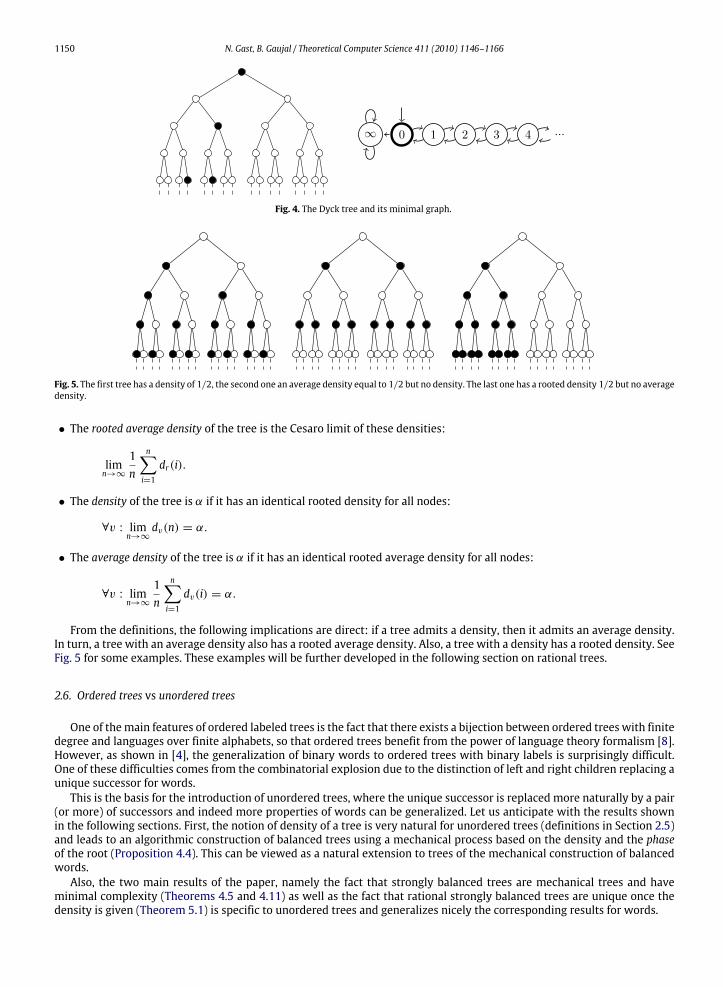
As for lower bounds on the complexity of a tree, it will be shown in Section 3 that trees such that PT (n) ≤ n for atleast one n are rational, i.e. have a bounded number of factors of any size (this implies that its minimal multigraph is finite).Therefore, trees T such that G(T ) are infinite and with a minimal complexity should satisfy PT (n) = n+ 1. These trees willbe called Sturmian trees by analogy with words. This definition is close to that of [4] for ordered trees. It is not difficult toexhibit such trees. For example, for any Sturmianwordw, a d-ary tree such that all nodes on level i have labelwi is Sturmian.Another more interesting example is the Dyck tree, represented on Fig. 4. This tree is the unordered version of the tree-

automata recognizing the Dyck language (language generated by the context-free grammar S → aSbS|ε), introduced in [4]and it is not hard to see that this tree is Sturmian. For that, consider the graph G(T ) associated with the Dyck tree T , alsodisplayed in Fig. 4. There are two factors of height 1 in T : those with a root labeled 1 (all associated with node 0 in G(T ))and those with a root labeled 0 (associated with nodes∞, 1, 2, . . . in G(T )). This corresponds to the equivalence classesfor ≡1. All factors of height n with a root associated to nodes∞, n, n + 1, n + 2, . . . have labels equal to 0: no path oflength n in G(T ) reaches the only node with label 1, namely node 0. The factors of height n starting with a root i of G(T )with 0 ≤ i < n are distinct: their first node with label 1 is at level i+ 1. In other words, the equivalence classes for≡n are{∞, n, n+ 1, . . .}, {0}, {1}, . . . , {n− 1}. The number of distinct factors of height n is n+ 1.

2.5. Density

The density of a tree T is meant to capture the proportion of ones in the tree. For any node v and any height n ≥ 0, theproportion of nodes with label 1 in the factor of height n with root v is denoted by dv(n). Let r be the root of the tree T . Ifthe following limits exist, they define four notions of density:

• The rooted density of the tree is the limit of the density of the subtrees of the root r:

limn→∞

dr(n).


Fig. 4. The Dyck tree and its minimal graph.

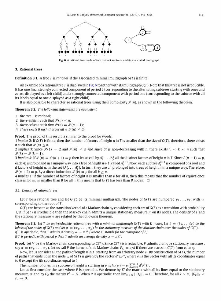
Fig. 5. The first tree has a density of 1/2, the second one an average density equal to 1/2 but no density. The last one has a rooted density 1/2 but no averagedensity.

• The rooted average density of the tree is the Cesaro limit of these densities:

limn→∞

1n

n∑i=1

dr(i).

• The density of the tree is α if it has an identical rooted density for all nodes:

∀v : limn→∞

dv(n) = α.

• The average density of the tree is α if it has an identical rooted average density for all nodes:

∀v : limn→∞

1n

n∑i=1

dv(i) = α.

From the definitions, the following implications are direct: if a tree admits a density, then it admits an average density.In turn, a tree with an average density also has a rooted average density. Also, a tree with a density has a rooted density. SeeFig. 5 for some examples. These examples will be further developed in the following section on rational trees.

2.6. Ordered trees vs unordered trees

One of themain features of ordered labeled trees is the fact that there exists a bijection between ordered trees with finitedegree and languages over finite alphabets, so that ordered trees benefit from the power of language theory formalism [8].However, as shown in [4], the generalization of binary words to ordered trees with binary labels is surprisingly difficult.One of these difficulties comes from the combinatorial explosion due to the distinction of left and right children replacing aunique successor for words.This is the basis for the introduction of unordered trees, where the unique successor is replaced more naturally by a pair

(or more) of successors and indeed more properties of words can be generalized. Let us anticipate with the results shownin the following sections. First, the notion of density of a tree is very natural for unordered trees (definitions in Section 2.5)and leads to an algorithmic construction of balanced trees using a mechanical process based on the density and the phaseof the root (Proposition 4.4). This can be viewed as a natural extension to trees of the mechanical construction of balancedwords.Also, the two main results of the paper, namely the fact that strongly balanced trees are mechanical trees and have

minimal complexity (Theorems 4.5 and 4.11) as well as the fact that rational strongly balanced trees are unique once thedensity is given (Theorem 5.1) is specific to unordered trees and generalizes nicely the corresponding results for words.


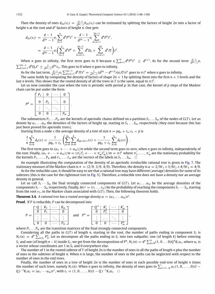
Fig. 6. A rational tree made of two distinct subtrees and its associated multigraph.

3. Rational trees

Definition 3.1. A tree T is rational if the associated minimal multigraph G(T ) is finite.

An example of a rational tree T is displayed in Fig. 6 togetherwith itsmultigraphG(T ). Note that this tree is not irreducible.It has one final strongly connected component of period 2 (corresponding to the alternating subtrees starting with ones andzeros, displayed as a left child) and a strongly connected component with period one (corresponding to the subtree with allits labels equal to one displayed as a right child).It is also possible to characterize rational trees using their complexity P (n), as shown in the following theorem.

Theorem 3.2. The following statements are equivalent

1. the tree T is rational;2. there exists n such that P (n) ≤ n;3. there exists n such that P (n) = P (n+ 1);4. There exists B such that for all n, P (n) ≤ B.

Proof. The proof of this result is similar to the proof for words.1 implies 2: If G(T ) is finite, then the number of factors of height n in T is smaller than the size of G(T ), therefore, there existsn such that P (n) ≤ n.2 implies 3: Since P (1) = 2 and P (n) ≤ n and since P is non-decreasing with n, there exists 1 < k < n such thatP (k) = P (k+ 1).3 implies 4: IfP (n) = P (n+ 1) = p then let us call by An1, . . . A

np all the distinct factors of height n in T . Since P(n+ 1) = p,

each Ani is prolonged in a uniqueway into a tree of height n+1, called An+1i . Now, each subtree An+1i is composed of a root and

d factors of height n, in the set {An1, . . . Anp}. In turn, they are all prolonged into trees of height n in a unique way. Therefore,

P (n+ 2) = p. By a direct induction, P (k) = p for all k ≥ n.4 implies 1: If the number of factors of height n is smaller than B for all n, then this means that the number of equivalenceclasses for≡n is smaller than B for all n, this means that G(T ) has less than B nodes. �

3.1. Density of rational trees

Let T be a rational tree and let G(T ) be its minimal multigraph. The nodes of G(T ) are numbered v1 . . . , vK , with v1corresponding to the root of T .G(T ) can be seen as the transition kernel of aMarkov chain by considering each arc ofG(T ) as a transitionwith probability

1/d. If G(T ) is irreducible then the Markov chain admits a unique stationary measure π on its nodes. The density of T andthe stationary measure π are related by the following theorem.

Theorem 3.3. Let T be an irreducible rational tree with a minimal multigraph G(T ) with K nodes. Let ` = (`1, . . . `K ) be thelabels of the nodes of G(T ) and let π = (π1, . . . , πK ) be the stationary measure of the Markov chain over the nodes of G(T ).If T is aperiodic, then T admits a density α = π`t (where `t stands for the transpose of `).If T is periodic with period p then T admits an average density α = π`t .

Proof. Let V be the Markov chain corresponding to G(T ). Since G(T ) is irreducible, V admits a unique stationary measure ,say π = (π1, . . . , πK ). Let us call P the kernel of this Markov chain: Pi,j = a/d if there are a arcs in G(T ) from vi to vj.Now, let us consider all the paths of length n in T , starting from an arbitrary node vi. By construction of G(T ), the number

of paths that ends up in the node vi of G(T ) is given by the vector dneiPn, where ei is the vector with all its coordinates equalto 0 except the ith coordinate, equal to 1.The number of ones in a subtree of height n starting in vi is hn(vi) = ei

∑n−1k=0 d

kPk`t .Let us first consider the case where P is aperiodic. We denote by Π the matrix with all its lines equal to the stationary

measure, π and by Dk the matrix Pk −Π . When P is aperiodic, then limk→∞ ||Dk||1 = 0. Therefore, for all k > n, ||Dk||1 <εn → 0.


Then the density of ones d2n(vi) = d−1d2n−1

h2n(vi) can be estimated by splitting the factors of height 2n into a factor ofheight n at the root and dn factors of height n. One gets

d2n(vi) =d− 1d2n − 1

ein∑k=1

dkPk`t +d− 1d2n − 1

ei2n−1∑k=n+1

dkPk`t ,

=d− 1d2n − 1

ei

( n∑k=1

dkPk +2n−1∑k=n+1

dkDk +2n∑

k=n+1

dkΠ)`t .

When n goes to infinity, the first term goes to 0 because ei∑nk=1 d

kPk`t ≤ dn+1. As for the second term d−1d2n−1

ei∑2n−1k=n+1 d

kDk`t ≤ 1d2n−1

d2nεn. This goes to 0 when n goes to infinity.

As for the last term, d−1d2n−1

ei∑2n−1k=n+1 d

kΠ`t = 1d2n−1

(d2n − dn+2)(eiΠ)`t goes to π`t when n goes to infinity.The same holds by computing the density of factors of shape 2n+ 1 by splitting them into the first n+ 1 levels and the

last n levels. This shows that the rooted density of all the trees in T is the same, equal to π`t .Let us now consider the case when the tree is periodic with period p. In that case, the kernel of p steps of the Markov

chain can be put under the form

Pp =

P1 0 · · · 0

0 P2. . . 0

.... . .

. . ....

0 0 . . . Pm

.The submatrices P1 . . . Pm are the kernels of aperiodic chains defined on a partition S1 . . . Sm of the nodes of G(T ). Let us

denote by α1 . . . αm the densities of the factors of height np, starting in S1 . . . Sm, respectively (they exist because this hasjust been proved for aperiodic trees).Starting from a node v the average density of a tree of size n = pqn + rn, rn < p is

1n

n∑k=0

dk(v) =1

pqn + rn

(qn∑a=0

p∑b=0

dap+b+r(v)+1

pqn + rn

rn∑k=0

dk(v)

).

The first term goes to (α1 + · · · + αm)/mwhile the second term goes to zero, when n goes to infinity, independently ofthe root. Finally, (α1 + · · · + αm)/m = (π ′1`

t1 + · · · + π

′m`tm)/m = π`

t where π ′1, . . . , π′m are the stationary probability for

the kernels P1, . . . , Pm and `1, . . . `m are the vectors of the labels in S1 . . . Sm. �

An example illustrating the computation of the density of an aperiodic irreducible rational tree is given in Fig. 7. Thestationarymeasure of theMarkov chain isπ = (2/9, 3/9, 4/9). Therefore, the density is α = 2/9`1+3/9`2+4/9`3 = 4/9.As for the reducible case, it should be easy to see that a rational treemay have different (average) densities for some of its

subtrees (this is the case for the rightmost tree in Fig. 5). Therefore, a reducible tree does not have a density nor an averagedensity in general.Let us call S1 · · · Sm the final strongly connected components of G(T ). Let α1 . . . αm be the average densities of the

components S1 · · · Sm respectively. Finally, let r = (r1 . . . rm) be the probability of reaching the components S1 · · · Sm startingfrom the root v1, in the Markov chain associated with G(T ). Then, the following theorem holds.Theorem 3.4. A rational tree has a rooted average density α = (α1, . . . αm)r t .Proof. If P is reducible, P can be decomposed into

P =

Q K1 · · · Km0 P1 · · · 0... · · ·

. . ....

0 0 · · · Pm

and Pn =

Q n K ′1 · · · K ′m0 Pn1 · · · 0... · · ·

. . ....

0 0 · · · Pnm

,where P1 . . . Pm are the transition matrices of the final strongly connected components.Considering all the paths in G(T ) of length n, starting in the root, the number of paths ending in component S` is

N`(n) = dn∑i∈S`Pn1i. Let us decompose all the paths ending in S` into two subpaths: one (of length k) before entering

S` and one (of length n− k) inside S`, we get from the decomposition of Pn, N`(n) = dn∑nk=0(1, 0 . . . 0)Q

kKù`, where u` isa vector whose coordinates are 1 in S` and 0 everywhere else.The number of 1 in the rooted subtree of T of height 2n is the number of ones in all the paths of length n plus the number

of ones in the subtrees of height n. When n is large, the number of ones in the paths can be neglected with respect to thenumber of ones in the end trees.Finally, the number of ones in a tree of height 2n is the number of ones in each possible end-tree of height n times

the number of such trees, namely N`(n). When n goes to infinity, the density of ones goes to∑

`=1...m α`(1, 0, . . . , 0)(I −Q )−1Kù` = (α1 · · ·αm)r t , with r` = (1, 0, . . . , 0)(I − Q )−1Kù`. �


Fig. 7. An irreducible aperiodic rational tree and its minimal graph. The stationary probabilities over the associated Markov chain are π = (2/9, 3/9, 4/9).The density of the tree is α = 4/9.

An example of a reducible rational tree is given in Fig. 6. The previous result can be used to compute its rooted averagedensity. The graph G(T ) has two final components, one aperiodic component with density 1 and another one with period 2with average density 1/2. Starting from the root, both components are reached with probability 1/2. Therefore, such a treehas an average rooted density α = 1/2.(1/2)+ 1/2 = 3/4.Also, it is not difficult to show that if all final components have a density (rather than an average density), then the tree

has a rooted density, given by the formula given by Theorem 3.4.Finally, it is fairly straightforward to prove that since the transition matrix P of the Markov chain associated with G(T )

has all its elements of the form a/d, then the stationary probabilities π as well as the average rooted density α of a rationaltree are rational numbers of the form c/bwith 0 ≤ c ≤ b ≤ dK+1. This fact will be used in the algorithmic Section 5 tomakesure that the complexities of the algorithms do not depend on the size of the numbers.

4. Balanced and mechanical trees

In this section, we introduce the notions of strongly balanced trees and mechanical trees and explore the relationsbetween them. In particular we will prove that in the irrational case they represent the same set of trees, giving us aconstructive representation of this class of trees. These results are very similar to the ones on words, which are summarizedbelow.

4.1. Sturmian, balanced and mechanical words

One definition of a Sturmian word uses the complexity of a word. The complexity of an infinite word w is a functionPw : N → N where Pw(n) is the number of distinct factors of length n of the word w. A word is periodic if there exists nsuch that Pw(n) ≤ n. Sturmian words are aperiodic words with minimal complexity, i.e such that for any n:

Pw(n) = n+ 1. (1)

If x is a factor ofw, its height h(x) is the number of letters equal to 1 in x. A balanced word is a word where the letters 1 aredistributed as evenly as possible:

∀x, y factors ofw, |x| = |y| ⇒ |h(x)− h(y)| ≤ 1. (2)

A mechanical word can be constructed using integer parts of affine functions. Let α ∈ [0; 1] and φ ∈ [0; 1). The lower (resp.upper) mechanical word of slope α and phase φ,w = w1w2 . . . (resp.w′ = w′1w

′

2 . . . ) is defined by:

∀i ≥ 1 wi = b(i+ 1)α + φc − biα + φc,w′i = d(i+ 1)α + φe − diα + φe.

(3)

These three definitions represent almost the same set of words. In the case of aperiodic words, they are equivalent: aword is Sturmian if and only if it is balanced and aperiodic if and only if it is mechanical of irrational slope. For periodicwords, there are similar relations:

• A rational mechanical word is balanced.• A periodic balanced word is ultimately mechanical.

A word is called ultimately mechanical if it can be written as xw where x is a finite word and w is a mechanical word. Anexample of a balanced word which is not mechanical (and just ultimately mechanical) is the infinite word only made ofzeros except for one letter 1. For a more complete description of Sturmian words, we refer to [16].

4.2. Balanced and strongly balanced trees

Using the two definitions of factors of a tree, we define two notions of balance for trees: the first one and probably themost natural one, is what we call balanced trees and the other one is called strongly balanced trees.


Definition 4.1 (Balanced and Strongly Balanced Trees). A tree is balanced if for all n ≥ 0, the number of nodes with label 1in any two factors of height n, differs by at most 1.A tree is strongly balanced if for all n, k ≥ 0, the number of nodes with label 1 in any two factors of height n and base k,

differs by at most 1.

As the name suggests, strong balance implies balance (by taking k = 0). Actually, this notion is strictly stronger (Section 6displays an example of a balanced tree that is not strongly balanced). Although the balance property is weaker and seemsmore natural for a generalization fromwords, the following mostly focuses on strongly balanced trees that have almost thesame properties as their counterparts on words.

4.2.1. Density of a balanced treeBefore beginning the full investigation of balanced trees, we start with a rather straightforward property: a balanced tree

has a density.Let us recall the definition of the density (Section 2.5): for all node v and all height n, we call hv(n) the number of 1 in

the factor of root v of height n and dv(n) the density of this factor, dv(n)def=

1S(n)hv(n). Using this notation, we can write the

following result.

Proposition 4.2 (Density of Balanced Tree). A balanced tree has a density α.Moreover for all nodes v and for all heights n:

|hv(n)− bS(n)αc| ≤ 1. (4)

Proof. Letmn be the minimal number of 1 in all factors of height n. Since the tree is balanced, for all nodes v and n ≥ 1:

mn ≤ hv(n) ≤ mn + 1. (5)

Now let us consider a factor of height n+k and root v. It can be decomposed into a factor of height k of root v and dk factors ofheight n at the leaves of the previous factor. The number of ones in these factors can be bounded by expressions dependingonmn andmk:

mk + dkmn ≤ mn+k ≤ mk + 1+ dk(mn + 1). (6)

The density of a factor of height n is mnS(n) ≤ dv(n) =hv(n)S(n) ≤

mn+1S(n) . Using these facts, we can bound dv(n+ k)− dv(n):

mn+kS(n+ k)

−mn + 1S(n)

≤ dv(n+ k)− dv(n) ≤mn+k + 1S(n+ k)

−mnS(n)

.

Using (6), the left inequality can be lower bounded by

(d− 1)(dkmn +mkdn+k − 1

−mn + 1dn − 1

)= (d− 1)

(mn +mk/dk

dn − 1/dk−mn + 1dn − 1

)≥ (d− 1)

(mndn − 1

−mn + 1dn − 1

)≥ −

1S(n)

.

The samemethod can be used to prove that dv(n+k)−dv(n) ≤ 1S(n) , which shows that for n big enough, |dv(n+k)−dv(n)|

is smaller than ε, regardless of k. Thus dv(n) is a Cauchy sequence and has a limit α = limn→∞ mnS(n) . Because of Eq. (5), this

limit does not depend on v and the tree has a density.Let us now prove that |dv(n) − bS(n)αc| ≤ 1: dividing the Inequality (6) by S(n, k) and taking the limit when k goes to

∞ leads to:

(d− 1)mn + αdn

≤ α ≤(d− 1)mn + 1+ α

dn.

This shows that: S(n)α − 1 ≤ mn ≤ S(n)α, which implies Eq. (4). �

Similar ideas can be used to show that Eq. (4) can be improved in the case of strongly balanced trees. In a strongly balancedtree, for all bases and heights k, n ≥ 0, the number of ones h(n, k) in a factor of height n and base k satisfies:∣∣h(n, k)− bS(n, k)αc∣∣ ≤ 1. (7)

This is false in general for balanced trees.


4.3. Mechanical trees

Building a balanced tree is not that easy. According to the formula (4), each factor of height n must have bαS(n)c orbαS(n)c + 1 or dαS(n)e − 1 nodes labeled one. This leads to the following construction, inspired by the construction ofmechanical words.

Definition 4.3 (Mechanical Tree). A tree is mechanical with density α ∈ [0; 1] if for all nodes v, there exists a phase φv ∈[0; 1) that satisfies one of the two following properties:

∀n : hv(n) =⌊S(n)α + φv

⌋, (8)

or ∀n : hv(n) =⌈S(n)α − φv

⌉. (9)

In the first case, φv is an inferior phase of v. In the second case, φv is a superior phase of v.

This definition suggests that the phases of all nodes could be arbitrary. In fact, we will see that there exists a uniquemechanical tree once the phase of the root is given. The second question raised by this definition is the existence anduniqueness of the phase: we call φv ‘‘a’’ phase of a node φv and not ‘‘the’’ phase of φv since there may exist several phasesleading to the same tree. This is further discussed at the end of this section.We begin by a characterization of mechanical trees.

Proposition 4.4 (Characterization of Mechanical Trees). Given α ∈ [0; 1] and φ ∈ [0; 1), there exists a unique mechanical treeof density α such that φ is an inferior (resp. superior) phase of the root.Moreover, if φ is an inferior (resp. superior) phase of a node then φ0 ≤ · · · ≤ φd−1 are inferior (resp. superior) phases of its d

children, with

φi =φ + α + i− bα + φc

d

(resp. φi =

φ − α + i− dα − φed

). (10)

Proof. The proofwill be done in two steps. First,wewill see that ifwe define the phases as in (10) then the tree ismechanical.Second, we will see that this is the only way to do so.

Existence. Let α ∈ [0; 1] and φ ∈ [0; 1). We want to build a mechanical tree whose root has an inferior phase φ (thecase of a superior phase if similar and is not detailed here). LetA be an infinite tree. To each node v, we associate a numberφv defined by:

• φroot = φ.• If the phase of a node v is φv , its d children satisfy Eq. (10).

Then we build a labeled tree by putting to each node v the label bα+ φvc. Let us prove by induction on n that the followingrelation holds.

For all v: hv(n) =⌊S(n)α + φv

⌋. (11)

By definition of the labels, (11) holds when n = 1. Let n ≥ 0 and let us assume that (11) holds for n. Let v be a node withphase φv and let φ0 . . . φd−1 be the phases of its children. We assume that α + φv < 1 , which means that the label of thenode is 0 (a similar calculation can be done in the other case (α + φv > 1)).Using the well-known formula

∑d−1i=0 bx+

idc = bdxc, we can compute hv(n+ 1):

hv(n+ 1) =d−1∑i=0

bS(n)α + φic

=

d−1∑i=0

⌊dn − 1d− 1

α +α + φ + id

⌋=

⌊d(dn − 1d− 1

α +α + φ

d

)⌋= bS(n+ 1)α + φc.

Therefore, (11) holds for all nwhich means that the tree is mechanical.Uniqueness. Now, letA be a mechanical tree of density α. Let v be a node and φ0, . . . , φd−1 be the phases of its children.

Let i and j be two children and let hi(n) be the number of ones in the ith subtree (of phase φi). We want to prove that either(for all n: hi(n) ≤ hj(n)) or (for all n: hi(n) ≥ hj(n)). If the two nodes are both inferior (resp. superior), this is clearly true:


hi(n) ≤ hj(n) if and only if φi ≤ φj (resp. φi ≥ φj). If i is inferior and j is superior, it is not difficult to show that φi < 1− φjimplies hi(n) ≤ hj(n) and φi ≥ 1− φj implies hi(n) ≥ hj(n).Therefore we can assume (up to an exchange of the order of the children) that for all n:

h0(n) ≤ h1(n) ≤ · · · ≤ hd−1(n).

Moreover as hd−1(n) − h0(n) ≤ 1, there exists k such that h0(n) = h1(n) = · · · = hk(n) < hk+1(n) = · · · = hd−1(n).As∑d−1i=0 hi(n) does not depend on φ0, . . . , φd−1, then for each n there is only one k that works and therefore there is only

one possibility for hi(n) for all n and all i. By induction of the depth of the children, this implies that for every node v′ in thesubtree of root v, hv′(n) is fixed and therefore the tree with root v is unique.As we have seen in the beginning of the proof, the phases φi defined in (10) provide correct values for hi(·). Therefore

such a phase φi is a possible phase for the ith child. �

This theorem shows that when the phase is fixed the tree is unique. The converse is false and one can find several phasesthat lead to the same tree (for example, when α = 0 all phases define the tree with label 0 everywhere) but we will shownext that the set of densities α for which the phases are not necessarily unique has Lebesgue measure zero.If for all n, S(n)α + φ 6∈ N, then bS(n)α + φc = dS(n)α + φ − 1e. In that case, if φ is an inferior phase of a node then

1− φ is a superior phase of the node. Therefore – except for particular cases – there exist at least two phases of a node: oneinferior and one superior. Let us now look at the possible uniqueness of the inferior phase.Let us denote frac(x) ∈ [0; 1) the fractional part of a real number x and let us consider the sequence {frac(S(n)α + φ)}n∈N.

If this sequence can be arbitrarily close to 0, thismeans that for allψ < φ, there exists k such that bS(k)α+ψc < bS(k)α+φcand ψ cannot be a phase of the tree. Also, if this sequence can be arbitrarily close to 1, then one can show similarly that forall ψ > φ, ψ is not a phase of the node. Conversely, if there exists δ > 0 such that frac(S(n)α + φ) > δ (resp.< 1− δ) forall n and if we set φ′ = φ − ε (resp. φ′ = φ + ε), with ε < δ, then bS(n)α + φc = bS(n)α + φ′c for all n.Thus, a phase φ is unique if and only if 0 and 1 are accumulation points of the sequence {frac(S(n)α + φ)}n.Let us call x def= 1

d−1α and ydef= φ − x and x1, . . . , xk, . . . (resp. y1, y2, . . . ) be the sequence of the digits of x (resp. y) in

base d (also called the d-decomposition). We want to study the sequence frac(S(n)α + φ) = frac(xdn − y).

xdn − y =n∑k=1

xkdn−k︸︷︷︸∈N

+

∞∑k=1

(xk+n − yk)d−k.

Therefore, frac(xdn − y) is arbitrarily close to 0 implies that for arbitrarily big k, there exists n such that

xn . . . xn+k−2 = y1 . . . yk−1, xn+k−1 > yk, or frac (xdn − y) = 0. (12)

Also, frac(xdn − y) is arbitrarily close to 1 which implies that for arbitrarily big k, there exists n such that

xn, . . . , xn+k−2 = y1, . . . , yn−1, xn+k−1 < yn,

or the d-development of y is finite (i.e.with only zeros after some point ` : y = y1, . . . , y`, 1, 0, 0 . . .) and that for arbitrarilybig k, there exists n such that

xn, . . . , xn+k−2 = y1, . . . , y`, 0, 1, . . . , 1. (13)

Using this characterization, three cases can be distinguished.

• If αd−1 is a number such that all finite sequences over 0, . . . , d − 1 appear in its d-decomposition, then every phase is

unique. In particular, all normal numbers2 in base d verify this property and it is known that almost every number in [0, 1]is normal (see [6] or [9]).• If α ∈ Q, then the sequence frac(S(k)α + φ)

)is periodic and there is no phase φ such that φ is unique.

• If α is neither rational nor has the property that all d-sequences appear in α, then some φ can be unique and some othersmay not. For example, for d = 2, if α is (in base 2) the number

α = 0.101100111000111100001111100000 . . . ,

then if frac(α − φ) = 0, φ is unique (because α satisfies both Eqs. (12) and (13)). However φ1 and φ2 such thatfrac(α − φ1) = 0.10100 and frac(α − φ2) = 0.1010 are equivalent (generate the same tree).Other examples of the same type are the rewind trees, drawn on Fig. 16. The sequence of digits in base 2 of the density

of such a tree is a Sturmian word. Half of the nodes of the tree are associated with node 0 in the minimal graph andtherefore could have the same phase whereas the phases computed using Eq. (10) are not all the same. Therefore, phasesare not unique here.

2 A number is normal in base d if all sequences of length k appear uniformly in its d-decomposition.


4.3.1. Phases of a treeLet us call Φv the set of numbers that can be phases of a node v and Φ the set of the possible phases of a tree. Φ is the

union of all possible phases of its nodes:Φ = ∪vΦv . The setΦ may be countable or uncountable. Countable for example iswhen α/(d− 1) is normal since there are at most as many phases as nodes. Uncountable for example is for the tree with alllabels 0, for which for each node, all phases in [0; 1)work.In all cases, the set of possible phases is dense is [0; 1). Indeed, at least all phases defined by the relation (10) are inΦ . If

φ is the phase of the root, then all nodes at level k have a phase which is the fractional part of:

φ+α+ikd +α+ik−1

d + · · · + α + i1d

= α

(1dk. . .1d

)+φ

dk+ikdk+ · · · +

i1d1, (14)

with 0 ≤ ij < d for all j. Conversely all of these numbers are the phases of some node at level k.As k goes to infinity and using a proper choice of i1, . . . , ik the fractional part of this number can be as close as possible

to any number in [0; 1]. Thus the set of phases of the tree is dense in [0; 1].If the density is p(d−1)

dn+k−dk(with n + k minimal) one can show that the set of all possible phases for a given node is

[dm−1d−1 α;min(

dm+1−1d−1 α, 1)) for somem ∈ 0, . . . , n+ k− 1. AsΦ is dense in [0; 1), it contains all these intervals. Therefore,

Φ = [0; 1) and the tree has exactly n+ k different factors of height greater than n+ k. Hence its minimal graph has exactlyn+ k nodes.

4.4. Equivalence between strongly balanced and mechanical trees

As seen in Section 4.1, there are strong relations between balanced and mechanical words. This part shows the sameresults between strongly balanced and mechanical trees. This result is formally stated in the following theorem.A tree is ultimately mechanical if all nodes are mechanical (i.e. satisfies Eqs. (8) or (9)), except finitely many.

Theorem 4.5. The following statements are true.

(i) A mechanical tree is strongly balanced.(ii) An irrational strongly balanced tree is mechanical.(iii) A rational strongly balanced tree is ultimately mechanical.

This theorem is the analog of the theorem linking balanced and mechanical words. The word 0k10∞ is balanced but notmechanical, only ultimately mechanical. Its counterpart for trees would be a tree with all labels equal to 0 except for onenode which has the label 1. The label 1 can be put as deep as desired, which shows that we cannot bound the size of the‘‘non-mechanical’’ beginning of the tree. A more complicated example is drawn in Fig. 8.Let us begin by the proof of the first part of the theorem:

Lemma 4.6. A mechanical tree is strongly balanced.

Proof. Let n, k ∈ N. For all nodes v, hv(n, k) is the number of 1 in the factor of height n and base k rooted in v. We want toprove that for all pairs of nodes v and v′: |hv(n, k)− hv′(n, k)| ≤ 1.By Proposition 4.4, we can assume that all phases of the tree are inferior (the casewhere all phases are superior is similar).

We call φ (resp. φ′) a phase of the node v (resp. v′).

hv(n, k)− hv′(n, k) =⌊dn+k − 1d− 1

α + φ

⌋−

⌊dk − 1d− 1

α + φ

⌋−

⌊dn+k − 1d− 1

α + φ′⌋+

⌊dk − 1d− 1

α + φ′⌋.

Using the well-known inequality x− x′ − 1 < bxc − bx′c < x− x′ + 1, one can show that

−2 < hv(n, k)− hv′(n, k) < 2.

As hv(n, k) and hv′(n, k) are integers, we have−1 ≤ hv(n, k)− hv′(n, )k ≤ 1 which ends the proof of the lemma. �

Wewill see in the next Section 4.5 that a strongly balanced tree is rational if and only if its density can be written as pS(n,k)

(p, k, n ∈ N), therefore we will do the proof of Theorem 4.5 distinguishing strongly balanced tree with density of this formfrom the others.

Lemma 4.7. IfA is a strongly balanced tree of density α which cannot be written as pS(n,k) (p, k, n ∈ N) thenA is mechanical.


Proof. Let τ be a real number and v a node. At least one of the two following properties is true:

∀n ≥ 1 : hv(n) ≤ bS(n)α + τc, (15)∀n ≥ 1 : hv(n) ≥ bS(n)α + τc. (16)

To prove this, assume that it is not true. Then there exists k, n such that hv(n) < bS(n)α + τc and hv(k) > bS(k)α + τc.In that case the number of 1 in the factor of height n and base n − k (or k, k − n if k > n) is hv(n) − hv(k) ≤bS(n)α + φc − bS(k)α + φc − 2 < dn−dk

d−1 α − 1 which violates Formula (7).Let us now define the number φ as the minimum τ that satisfies (15):

φ = infτ

{For all n : hv(n) ≤ bS(n)α + τc

}.

For all τ > φ, the Eq. (15) is true, while for all τ ′ < φ, the Eq. (16) is true. This means that for all ε > 0 and all n:

S(n)α + φ − ε − 1 ≤ bS(n)α + φ − εc ≤ hv(n) ≤ bS(n)α + φ + εc ≤ S(n)α + φ + ε. (17)

Taking the limit when ε tends to 0 shows that:

S(n)α + φ − 1 ≤ hv(n) ≤ S(n)α + φ. (18)

Therefore, unless S(n)α + φ ∈ N, hv(n) = bS(n)α + φc = dS(n)α + φ − 1e.If there exists n ∈ N such that S(n)α + φ ∈ N, then, as α /∈ { p

S(n,k) , p, k, q ∈ N}, there are no other k ∈ N (k 6= n) suchthat S(k)α + φ ∈ N. If for this particular n hv(n) = S(n)α + φ = bS(n)α + φc, the node is inferior of phase φ. Otherwise,hv(n) = S(n)α + φ − 1 = dS(n)α + φ − 1e and the node is superior of phase 1− φ. �

Lemma 4.8. Let A be a strongly balanced tree such that there exist n and k such that all factors of shape (n, k) have the samenumber of nodes with label 1. Then the tree is mechanical.

Proof. Let us take n and k satisfying the property, such that n + k is minimal and let p be the common number of ones inthe factors of shape (n, k). Obviously, the tree has a density α = p(d−1)

dk(dn−1).

Let v be the root of the tree. The same proof as in the irrational case can be used to establish that there exists φ such that

S(n)α + φ − 1 ≤ hv(n) ≤ S(n)α + φ,

and that the root is inferior of phase φ if there is no j such that hv(j) = dj−1d−1 α+φ−1 — resp. superior of phase 1−φ if there

is no i such that hv(i) = di−1d−1 α+ φ. Therefore the tree is mechanical unless there exist i and j satisfying these equalities. Let

us show that if there exist such i and j, there is a contradiction.Let i = mini′{hv(i′) = di

′−1d−1 α + φ} and j = minj′{hv(j

′) = dj′−1d−1 α + φ − 1}. Either i < j or i > j, let us assume that j < i,

the other case is similar. The number of ones in the factor of height i− j and base j is p′ = di−djd−1 α + 1. In that case we have

i ≥ k + n, otherwise this would violate the minimal property of n + k. If j − i > n the factor of height i − j and base j iscomposed of a factor of height i− n and base j and di−n−k factors of height n and base k – that have exactly p nodes labeledone as assumed in the previous paragraph – and then the number of 1 in this subtree is:

hv(i)− hv(j)− di−n−kp+ φ + 1 = αdi−n − dj

d− 1+ φ + 1,

which violates the minimality of i.Then if all factors of shape (k, n) have exactly p nodes labeled 1, the tree is mechanical. �

Lemma 4.9. If A is a strongly balanced tree with a density α = pS(n,k) then it has at most n factors of shape (n, k) with p + 1

ones or p− 1 ones.

Proof. Using Eq. (7), each factor of shape (n, k) has p − 1, p or p + 1 nodes labeled by 1. As the tree is strongly balanced,either there is no factor with p− 1 ones or no factor with p+ 1 ones. Let us assume that there is no factor with p− 1 ones(the other case is similar). We claim that there are at most n factors of shape (n, k)with p+ 1 nodes labeled by 1.Indeed, let f be a factor of shape (n′, k′) with n′ = `n, i ∈ N, k′ ≥ k. This tree is composed of j blocks of shape (n, k)

(where j depends on ` and k′) and using Eq. (7) again, the number of nodes with label 1 is either jp−1, jp or jp+1. Thereforeat most one of the (n, k) blocks has p+ 1 nodes labeled by 1.If there were more than n+ 1 blocks of shape (n, k)with p+ 1 ones in the whole tree, starting respectively at line l1, . . .

and ln+1, there would be two blocks with li = lj mod n and the block of height lj − li + n, li would have jp+ 2 ones, whichis not possible. Therefore there are at most n blocks of shape n, kwith p+ 1 nodes labeled by 1 in the whole tree. �

An example of a rational tree strongly balanced but not mechanical is presented in Fig. 8.

Lemma 4.10. A strongly balanced tree with density α = pS(n,k) , p, n, k ∈ N, is ultimately mechanical. Furthermore, if the tree is

irreducible, it is mechanical.


Fig. 8. Example of a rational tree that is strongly balanced but not mechanical. On the left is the tree itself. In the middle the mechanical suffixes of thetree are displayed and its minimal graph (reducible) is displayed on the right. There is one strongly connected component – the one corresponding to thenodes 3-4 – and two corresponding suffixes: A3 , starting with a 0, and A4 , starting with a 1. One can verify on the picture that the beginning of this treeis strongly balanced and as it continues with density exactly 1/3, the whole tree is strongly balanced. However this tree is ultimately mechanical but notmechanical since in a mechanical tree of density 1/3, all factors of height 2 should have b1+ φc = 1 node labeled by one.

Proof. Using Lemma 4.9, there are at most n factors of height n and base kwith p+ 1 nodes labeled 1, in the rest of the treeall factors of shape (n, k) have exactly p ones. Then the tree is ultimately mechanical by Lemma 4.8.If the tree is irreducible, a factor appears either 0 or an infinite number of times. As there are at most n factors of shape

(k, n)with p+ 1 nodes labeled 1, there are no such factors and the tree is mechanical by Lemma 4.8.Note that this lemma concludes the proof of Theorem 4.5. �

4.5. Link with Sturmian trees

In the case of words, Sturmian words are exactly the balanced (or mechanical) aperiodic words. The case of trees doesnot work as well since the Dyck Tree (Fig. 4) andmore generally all examples of Sturmian trees given in [4] are not balanced.However, the reverse implication holds as seen in the following theorem:

Theorem 4.11. The following propositions are true.

• A strongly balanced tree of density different from pS(n,k) (for any p, n, k ∈ N) is Sturmian.

• A strongly balanced tree of density pS(n,k) (p, n, k ∈ N) is rational.

This result has a simple implication: a strongly balanced tree is rational if and only if there exist p, n, k ∈ N such that itsdensity is p

S(n,k) .

Proof. Let us consider the case of inferior mechanical trees (the superior case being similar).LetA be a mechanical tree of density α, let v be a node and let n ≥ 0. According to Proposition 4.4, the factor of root v of

height n only depends on the phase φv of its root. In fact, one can show in the proof of Proposition 4.4 that this factor onlydepends on the values b d

i−1d−1 α+φvc (1 ≤ i ≤ n). If we write fi(φ)

def= b

di−1d−1 α+φc (i ≥ 0, φ ∈ [0 : 1]), the number of factors

of height n only depends on the values f1(φ) . . . fn(φ).As seen in (14), the set of phases is dense in [0; 1], therefore they are exactly as many trees as tuples f1(φ), . . . , fn(φ)

when φ ∈ [0; 1) by right-continuity of fi.Each fi is an increasing functions taking integer values and hi(1)−hi(0) = 1. Thus there are at most n+1 different tuples

and then at most n+ 1 factors of height n and a mechanical tree is either rational or Sturmian.Moreover if α 6∈

{p

dkS(n)/p, n, k ∈ N

}, we cannot have i 6= j and d

i−1d−1 α + φ,

dj−1d−1 α + φ ∈ N and then there are exactly

n+ 1 factors of height n.If α = p

S(n,k) , then the number of factors of height n is at most n. Therefore the tree is rational using Theorem 3.2 (seeSection 4.3.1).If the tree is not mechanical, then Theorem 4.5 says that the tree has a density α = p

S(n,k) and is ultimately mechanical:there exists a depth D ≥ 1 after which the tree is mechanical. Therefore, there are at most S(D) + n factors of any height(n in the mechanical children because of the value of α plus S(D) in the prefix subtree). In that case the tree is rational byTheorem 3.2. �

5. Algorithmic issues

5.1. Testing if a rational tree is strongly balanced

Given a finite description of a rational tree, let us consider the problem of checkingwhether this tree is strongly balanced.An algorithm that works in time 0(N3)where N is the number of vertices of the minimal graph of the tree is presented.The first focus is on the description of the special structure of the minimal graph of a rational strongly balanced tree.

Then an algorithm for irreducible rational trees is described as well as a sketch of the algorithm for the general case.


Fig. 9. All mechanical trees of the same density α have the same minimal graph Gα . These graphs represent Gα for α = 1/3, 1/7, 4/15 and 6/15 = 2/5.For all graphs with n nodes, there are exactly n different mechanical trees of this particular density, depending on which node is associated to the root.Note that the first three graphs have a very similar structure (Fig. 16 displays more mechanical trees with this structure).

Fig. 10. General form of the graph of a reducible strongly balanced tree: an acyclic graph ending in a unique strongly connected component.

5.1.1. Graphs of rational strongly balanced treesThe aim of this section is to study the general form of the minimal graphs of rational strongly balanced trees. In fact, we

will see that they have a very particular form. Themain results of this section are summarized in Theorem 5.1 and illustratedby Figs. 9 and 10.

Theorem 5.1. (i) Two rational mechanical trees of the same density α have the same minimal graph Gα , up to the choice of theinitial node of this graph. Moreover Gα is irreducible.

(ii) The minimal graph of a strongly balanced tree of density α has a unique strongly connected component that is final, Gα .

Proof. (i) Let us first consider a rational mechanical tree of density α. We know that there exist p, k, n ≥ 0 such thatα =

p(d−1)dk(dn−1)

. Using Section 4.3.1, the minimal graph has exactly n + k nodes, and for any node, the set of all possiblephases of all its descendants is [0; 1). Therefore, the graph is strongly connected and unique. The only difference betweentwo rational mechanical trees of the same density is to which node the root of the tree is associated. Fig. 9 displays severalexamples. The (unique) minimal graph of the mechanical trees of density 1/3, 1/7, 4/15 and 2/15 are displayed.(ii) If the tree is strongly balanced but not mechanical, it is ultimately mechanical (see Proposition 4.10) which means

that after a finite depth k, all suffixes are mechanical trees with the same density. All of these trees have the same graph,therefore theminimal graph has a unique final strongly connected componentwhich is reached in atmost k steps. Therefore,theminimal graph of a strongly balanced tree can be decomposed into a finite acyclic graph and one final strongly connectedcomponent, like in Fig. 10. �

5.1.2. Irreducible treesTesting if two graphs with a given fixed out-degree are isomorphic can be done in polynomial time [17]. Therefore using

the result shown in the previous Section 5.1.1, an algorithm to test if a graph represents a mechanical tree can be obtainedby computing the density α of the graph and testing if the graph is isomorphic to the graph of all mechanical trees withdensity α. However this is not very efficient and here we propose an algorithm that tests the balance property directly.Consider an irreducible rational treeA and let n0 be the number of vertices of its minimal graph. Theorem 4.11 says that

it is strongly balanced if and only if it is mechanical. In that case its density is pS(n0,k0)

for some p, k0 ∈ N and all subtrees ofshape (k0, n0) have exactly p nodes with label 1. Such factors will be called basic blocks in the following.Recall that the tree is strongly balanced if all factors of shape (n, k) have bαS(n, k)c or bαS(n, k)+ 1c nodes of label one.

We want to show that testing it for all n, k < n0 + k0 is sufficient.Let v be a node and n, k ≥ 0 and let hv(F) be the number of labels 1 in the factor F of shape (n, k)with root v.Starting from F , we construct a new factor F ′ by adding a new factor on top of F of shape n0, k − n0. This new factor

can be partitioned into dk−n0−k0 basic blocks. The total factor F ′ is of shape (n + n0, k − n0) and its number of ones ishv(F ′) = hv(F)+ dk−n0−k0p (see Fig. 11).The augmentation of the factor can be repeated until its shape n′, k′ is such that k′ ≤ k0 + n0. Its number of ones is

hv(F ′) = hv(F)+ H where H does not depend on v.The second phase consists of building a new factor F ′′ by removing a factor from F ′ of shape n0, k′+n′−n0. The removed

part can be partitioned into dn′−n0−k0 basic blocks. Therefore the number of ones in F ′′ is hv(F ′′) = hv(F ′)− dn

′−n0−k0p. This

transformation is illustrated in Fig. 12.By repeating this transformation as long as n′′ > n0+k0, we get a final factor F ′′whose shape is (n′′, k′′)with n′′ < n0+k0,

k′′ < n0+ k0 and whose number of ones is hv(F ′′) = hv(F)+H−K , where H and K do not depend on v but only on n and k.


Fig. 11. The first transformation: if k > n0 + k0 , we add a level of factors of shape n0, k0 that all contain exactly p ones. The shape of the factor becomes(n+ n0, k− n0). We repeat the transformation until the shape is (n′, k′)with k′ < n0 + k0 . In the figure, Tk stands for pdk−n0−k0p.

Fig. 12. The second transformation: if n′ > n0 + k0 , we can remove a level of factors of shape (n0, k0). The shape of the factor becomes (n′ − n0, k′). Werepeat the transformation until the shape is (n′, k′)with n′ < n0 + k0 (here, Tn′ = pdn

′−n0−k0 ).

Since hv(F) = hv(F ′′) − H + K , it is enough to compute the number of ones in all factors with shape (n′′, k′′) wheren′′ < n0 + k0, k′′ < n0 + k0, to be able to obtain the number of ones in all factors on any shape.Also, it is enough to test if all factors with shape (n′′, k′′) where n′′ < n0 + k0, k′′ < n0 + k0 satisfy the strong balance

property for all factors on any shape to have the same property.There are at most n factors of a given height and base. For b < m, let us call hi,h,m the number of 1 in the ith factor of

height b and base b + m. Let us call v(i) = (v1(i), . . . , vd(i)) the set of the d children of the tree rooted in i. hi,b,m can becomputed using the formula:

hi,b,m =

hi,1,0 = `(i)hi,b,0 = `(i)+∑j∈v(i) hj,b−1,0

hi,b,m =∑j∈v(i) hj,b−1,m−1.

(19)

These considerations yield the Algorithm 1. The main steps of the algorithm are:

1. Compute the density α of the tree (cf Theorem 3.4).2. If α cannot be written as p d−1

dN−dk, the tree is not strongly balanced.

3. Check the strongly balanced property on the factors of shape (n, k) < (N,N).

Solving the Markov chain to get α takes at most O(N3) operations. Writing the density under the form pdN−dk

is linear inN and computing all hi,b,m takes O(N3) operations using the formula (19). Therefore the algorithm runs in time O(N3).

5.1.3. General caseThe general case is more complicated since there can be some factors of shape (n0, k0)with p+1 (or p−1) nodes labeled

by 1. However the structure of the minimal graph of strongly balanced trees made in Section 5.1.1 can be useful.

• Indeed, the minimal graph must have only one strongly connected component and it must correspond to a stronglybalanced tree.• If the density of the strongly connected component is p

2n0Ck0, all factors of shape n0, k0 in the strongly component have

exactly p nodes labeled by 1.

Therefore, using the same techniques of reduction of the size as in Fig. 11, one can show that we just have to test thebalanced property for factors of shape at most (N,N)where N is the number of vertices in the graph.


Algorithm 1 Testing if an irreducible rational tree is strongly balancedRequire: Minimal graph G of an irreducible rational treeEnsure: The tree corresponding to G is strongly balancedN:= number of vertices of GCompute the density α of the Markov Chainif for all k: d

N−dkd−1 α 6∈ N then

return ‘‘not strongly balanced’’end iffor 1 ≤ i, n, k ≤ N doCompute hi,n,k according to (19)if hi,n,k 6= b d

n−dkd−1 αc and hi,n,k 6= b

dn−dkd−1 αc + 1 then

return ‘‘not strongly balanced’’end if

end forreturn ‘‘strongly balanced’’

5.2. Counting

In this part, we address the problem of counting all possible factors of a mechanical tree. Wewill focus on trees of degree2 and will compare this to the total number of possible factors of binary trees.There are 2n finite words on a binary alphabet of length n. Not all these words can be factors of a Sturmian words, for

example 0011 cannot since it is not balanced. In fact, the number of factors of length n of Sturmian words (see for example[5]) is:

1+n∑i=1

(n− i+ 1)φ(i), (20)

where φ is the Euler function (φ(i) is the number of integers less than i and coprime with i). Asymptotically, the number offactors is equivalent to n3/π2.The number an of unordered complete binary trees of height n satisfies the equation:

an+1 = an(an + 1). (21)

According to [19], there is no simple solution of this equation but using the method described in [1], one can show thatan is the nearest integer close to θ2

n− 1/2, where θ ≈ 1.597910218 . . . is the exponential of the rapidly convergent series

ln(3/2)+∑n≥0 ln(1+ (2an + 1)

−2).In Section 4.5, we have seen that the number of factors of height n of a mechanical tree is the number of tuples

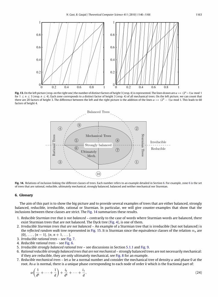
(f1(φ, α), . . . , fn(φ, α))where fi(φ, α) = b(2n − 1)α + φc. Let us call un this number.To count the number of these tuples, consider the lines α 7→ (2n− 1)α mod 1, with 0 ≤ α ≤ 1 (see Fig. 13). The number

of tuples is the number of different zones in this figure.An exact computation of un is cumbersomebut good bounds can be computed easily. un+1−un corresponds to the number

of zones added by adding the lines α 7→ (2n+1 − 1)α − i. Each of these 2n+1 − 1 lines:

• adds at least a new zone if it only crosses other lines at points φ = 0 or φ = 1. This is a very low estimate since it is onlytrue for i = 0 or i = 2n − 2, in the other cases it crosses at least the line α 7→ φ.• adds at most 1+ n zones if it crosses the n lines corresponding to α 7→ (2j − 1)α − ij, 1 ≤ j ≤ n and if all these pointsare pairwise distinct.

Therefore we have an estimation for all n ≥ 2:

2+ 2(2n+1 − 3) ≤ un+1 − un ≤ (n+ 1)(2n+1 − 1). (22)

This leads to the bounds for n ≥ 3:

2n+2 ≤ un ≤ n2n+1. (23)

Improving these bounds seems difficult. To do so, one would have to count whether a ‘‘new’’ intersection has alreadybeen counted or if it is on the boundary φ = 0. By simulation, it seems that the number of trees is closer to n2n+1 than to2n+1.


1

1

0.8

0.8

0.6

0.6

0.4

0.4

0.2

0.20

1

0.8

0.6

0.4

0.2

00 10.80.60.40.20

Fig. 13.On the left picture (resp. on the right one) the number of distinct factors of height 3 (resp. 4) is represented. The lines drawnareα 7→ (2n−1)α mod 1for 1 ≤ n ≤ 3 (resp. n ≤ 4). Each zone corresponds to a distinct factor of height 3 (resp. 4) of all mechanical trees. On the left picture, we can count thatthere are 20 factors of height 3. The difference between the left and the right picture is the addition of the lines α 7→ (24 − 1)α mod 1. This leads to 60factors of height 4.

Fig. 14. Relations of inclusion linking the different classes of trees. Each number refers to an example detailed in Section 6. For example, zone 6 is the setof trees that are rational, reducible, ultimately mechanical, strongly balanced, balanced and neither mechanical nor Sturmian.

6. Glossary

The aim of this part is to show the big picture and to provide several examples of trees that are either balanced, stronglybalanced, reducible, irreducible, rational or Sturmian. In particular, we will give counter-examples that show that theinclusions between these classes are strict. The Fig. 14 summarizes these results.

1. Reducible Sturmian tree that is not balanced – contrarily to the case of words where Sturmian words are balanced, thereexist Sturmian trees that are not balanced. The Dyck tree (Fig. 4), is one of them.

2. Irreducible Sturmian trees that are not balanced – An example of a Sturmian tree that is irreducible (but not balanced) isthe reflected random walk tree represented in Fig. 15. It is Sturmian since the equivalence classes of the relation≡n are{0}, . . . , {n− 1}, {n, n+ 1, . . . }.

3. Irreducible rational trees – see Fig. 7.4. Reducible rational trees – see Fig. 6.5. Irreducible strongly balanced rational tree – see discussions in Section 5.1.1 and Fig. 9.6. Rational reducible strongly balanced trees that are notmechanical – strongly balanced trees are not necessarilymechanical:if they are reducible, they are only ultimately mechanical, see Fig. 8 for an example.

7. Reducible mechanical trees – let α be a normal number and consider the mechanical tree of density α and phase 0 at theroot. As α is normal, there is a unique phase corresponding to each node of order kwhich is the fractional part of:

α

(1dk+ · · · +

1d

)+ikdk+ · · · +

i1d, (24)


Fig. 15. The reflected randomwalk tree: each node of type n is followed by one of type n−1 and one of type n+1 (except for 0 that is followed by 0 and 1).

Fig. 16. Example of the restart tree corresponding to the word aabaaab . . . .

Fig. 17. Number of ones in a factor of the restart tree of height 5.

for a unique sequence i1, . . . , ik (see the end of Section 4.3 for details about normal numbers and phases). If two phasescorresponding to i1, . . . , ik and i′1, . . . , i

′

k′ are equal, then we have

frac

(α

(1dk+ · · · +

1dk′+1

)+

k∑j=1

ijdj−

k′∑j=1

i′jdj

)= 0.

As α is normal, it is irrational. Therefore k = k′ and frac(∑j≤k

ijdj−∑j≤k′

i′jdj) = 0. By uniqueness of the decomposition of

a number in base d, this implies that the two sequences are equal. This shows that two different nodes in the tree have adifferent phase. Thus the minimal graph of this tree is exactly the tree itself which is in a sense the most reducible tree.

8. Irreducible mechanical trees – letw be a mechanical word and consider a graph with vertices {0, 1, . . . , }, where a nodei ≥ 0 has label one if and only ifwi = 1. The node i has two outgoing arcs: one ending in i+ 1, one ending in 0. We callthis graph a restart tree since for a node n, we have the choice between restarting back in 0 or continuing in n + 1, anexample is displayed in Fig. 16.As seen in Fig. 17, the number of ones in a factor of height n that corresponds to the node i is

hi(n) = wi + · · · + wi+n−1 + h0(n− 1)+ · · · + h0(1), (25)

and the number of ones in a factor of height n and base k is

hi(n, k) = hi(n)− hi(k) = wk + · · · + wi+n−1 + h0(n− 1)+ · · · + h0(k). (26)

Therefore the tree is strongly balanced if and only if the word w is balanced. Since the tree is irreducible, in that casethe tree is also mechanical. Moreover one can show that for any wordw the tree has a density which is limn→∞

h0(n)2n−1 =

w02 +

w14 +

w28 + · · · .

Thus for any aperiodic balanced word, this provides an example of an irreducible irrational strongly balanced tree.9. Rational balanced tree that is not strongly balanced – An example of a rational tree that is balanced but not stronglybalanced is presented in Fig. 18. One can show that all of its factors of height 3 have exactly 4 nodes with label one.Using this fact, one can show that the number of ones in a factor of height 3n+ i (0 ≤ i ≤ 3) rooted in a node j is:

Height Node 1 Node 2 Node 3 Node 43n 4 8

n−17 4 8

n−17 4 8

n−17 4 8

n−17

3n+ 1 1+2.4 8n−17 0+ 2.4 8

n−17 0+ 2.4 8

n−17 1+2.4 8

n−17

3n+ 2 1+4.4 8n−17 1+ 4.4 8

n−17 2+ 4.4 8

n−17 2+4.4 8

n−17


Fig. 18. A rational balanced tree that is not strongly balanced.

This shows that the tree is balanced. It is not strongly balanced since there are factors of shape (1, 1) with 2 nodeslabeled by one and others with 0 nodes labeled by one as seen in the bottom right part of Fig. 18. Also its minimalgraph is not isomorphic to the unique minimal graph of a mechanical tree of density 4/7 that has only 3 nodes (see thediscussion about graphs of strongly balanced tree in Section 5.1.1).

10. Irrational balanced tree that is not strongly balanced – Building an irrational tree not strongly balanced requires morework. We consider a tree which has a root r labeled by 0 and two children that are mechanical trees of density α andrespective phases φ and φ+ a. We will see that under some conditions on α, φ and a, this will be an irrational tree thatis balanced but not strongly balanced nor rational, nor Sturmian.

The two children of the root are balanced trees which means that the tree is balanced if and only if for all n:

b(2n+1 − 1)αc ≤ hr(n+ 1) ≤ b(2n+1 − 1)αc + 1. (27)

Let us call k = b(2n − 1)α + φc and x = frac((2n − 1)α + φ).

hr(n+ 1) = b(2n − 1)α + φc + b(2n − 1)α + φ + ac= k+ bk+ x+ ac.

As (2n+1 − 1)α = 2k+ 2x+ α − 2φ, the Eq. (27) holds if for all x ∈ [0; 1), we have:

0 ≤ k+ bk+ x+ ac − b2k+ 2x+ α − 2φc ≤ 1.

which holds if for all x ∈ [0; 1):

0 ≤ bx+ ac − b2x+ α − 2φc ≤ 1.

This equation is satisfied if and only if

(x+ a < 1 and − 1 ≤ 2x− 2φ + α < 1) or (x+ a ≥ 1 and 0 ≤ 2x− 2φ + α < 2).

Looking at the extremal cases for x+ a < 1 and x+ a ≥ 1 which are x = 0, 1− a, 1, one gets 4 relations:

2(1− a)− 2φ + α < 1−1 ≤ −2φ + α2− 2φ + α < 20 ≤ 2(1− a)− 2φ + α.

Therefore the tree is balanced if and only if

α

2< φ ≤

α + 12

< φ + a < 1. (28)

Moreover if α + φ ≥ 1 and 3α + φ < 2, the tree is not strongly balanced since its beginning is

There are lots of triples α, φ, a satisfying conditions (28). For example a tree with α = 13 + ε, φ = 0.6 and a = 0.2

where ε ∈ R \ Q with ε small enough (for example ε < 0.01 works since α2 ≈ 0.21 < 0.6 <α+12 ≈ 0.71 ≤ 0.8 < 1

and α + φ > 1, 3α + φ ≈ 1.9 < 2).


References

[1] A.V. Aho, N.J.A. Sloane, Some doubly exponential sequences, Fibonacci Quarterly 11 (4) (1973) 429–437.[2] E. Altman, B. Gaujal, A. Hordijk, Discrete-Event Control of Stochastic Networks: Multimodularity and Regularity, in: LNM, vol. 1829, Springer-Verlag,2003.

[3] J. Berstel, Sturmian and episturmian words (a survey of some recent result results), in: G. Rahonis, S. Bozapalidis (Eds.), Conference on AlgebraicInformatics, in: Lecture Notes Comput. Sci., vol. 4728, 2007, pp. 23–47.

[4] J. Berstel, L. Boasson, O. Carton, I. Fagnot, Sturmian trees, Theory of Computing Systems (2009) 1–36.[5] J. Berstel, M. Pocchiola, Random generation of finite sturmian words, in: LIENS - 93 -8, DMI, ENS, LITP - Institute Blaise Pascal, 1993.[6] E. Borel, Les probabilités dénombrables et leurs applications arithmétiques, Rendiconti del Circolo Matematico di 27 (1909) 247–271.[7] J. Cassaigne, Double sequences with complexitymn+ 1, Journal of Automata, Languages and Combinatorics 4 (3) (1999) 153–170.[8] B. Courcelle, Fundamental properties of infinite trees, Theoretical Computer Science 25 (2) (1983) 95–169. Fundamental study.[9] R. Durrett, Probability: Theory and Examples, Wadsworth & Brooks/Cole, 1991.[10] T. Fernique, Pavages, Fractions continues et géométrie discrète, Ph.D. Thesis, University of Montpellier, 2007.[11] N. Gast, B. Gaujal, Balanced labeled trees: Density, complexity and mechanicity, in: Words, 6th international conference on words, Marseille, France,

2007.[12] B. Gaujal, A. Hordijk, D. Van der Laan, On the optimal open-loop control policy for deterministic and exponential polling systems, Probability in

Engineering and Informational Sciences 21 (2007) 157–187.[13] B. Gaujal, E. Hyon, Optimal routing policy in two deterministic queues, Calculateurs Parallèles (2001).[14] B. Hajek, Extremal splittings of point processes, Mathematics of Operation Research 10 (4) (1985) 543–556.[15] R. Klette, A. Rosenfeld, Digital straightness— a review, Discrete Applied Mathematics 139 (2004) 197–230.[16] M. Lothaire, Algebraic Combinatorics on Words, Cambridge University Press, New York, 2002.[17] E. Luks, Isomorphism of graphs of bounded valence can be tested in polynomial time, Journal of Computer and System Sciences 25 (1982) 42–65.[18] M. Morse, G.A. Hedlund, Symbolic dynamics ii. sturmian trajectories, American Journal of Mathematics 62 (1940) 1–42.[19] N.J.A. Sloane, et al. The on-line encyclopedia of integer sequences, 2009. URL www.research.att.com/~njas/sequences/.

http://www.research.att.com/~njas/sequences/

Documents

Infinite labeled trees: From rational to Sturmian trees