inferences on stress-strength reliabilityfrom lindley distributions

D.K. Al-Mutairi†, M.E. Ghitany† & Debasis Kundu‡

Abstract

This paper deals with the estimation of the stress-strength parameter R = P (Y < X)when X and Y are independent Lindley random variables with different shape param-eters. The uniformly minimum variance unbiased estimator has explicit expression,however, its exact or asymptotic distribution is very difficult to obtain. The maximumlikelihood estimator of the unknown parameter can also be obtained in explicit form.We obtain the asymptotic distribution of the maximum likelihood estimator and it canbe used to construct confidence interval of R. Different parametric bootstrap confi-dence intervals are also proposed. Bayes estimator and the associated credible intervalbased on independent gamma priors on the unknown parameters are obtained usingMonte Carlo methods. Different methods are compared using simulations and one dataanalysis has been performed for illustrative purposes.

Key Words and Phrases Lindley distribution; Maximum likelihood estimator; Asymp-

totic distribution; Uniformly minimum variance unbiased estimator; Prior distribution; Pos-

terior analysis; Credible intervals.

† Department of Statistics and Operations Research, Faculty of Science, Kuwait University,

P.O. Box 5969 Safat, Kuwait 13060; e-mails: dhaif@stat.kuniv.edu & meghitany@yahoo.com.

‡Department of Mathematics and Statistics, Indian Institute of Technology Kanpur, Pin

208016, India; e-mail: kundu@iitk.ac.in.

1

2

1. Introduction

The Lindley distribution was originally proposed by Lindley (1958) in the context of Bayesian

statistics, as a counter example of fudicial statistics. The Lindley distribution has the fol-

lowing probability density function (PDF)

f(x; θ) =θ2

1 + θ(1 + x)e−θx, x > 0, θ > 0. (1)

From now on if a random variable (RV) X has the PDF (1), then it will be denoted by

Lindley(θ). The corresponding cumulative distribution function (CDF) and hazard rate

function (HRF) are

F (x; θ) = 1−(1 +

θ

1 + θx

)e−θx, (2)

and

h(x; θ) =f(x; θ)

1− F (x; θ)=

θ2(1 + x)

1 + θ(1 + x), (3)

respectively. Ghitany et al. (2008) showed that the PDF of the Lindley distribution is

unimodal when 0 < θ < 1, and is decreasing when θ ≥ 1. They have also shown that the

shape of the HRF of the Lindley distribution is an increasing function and the mean residual

life function

µ(x) = E(X − x|X > x) =1

θ+

1

θ(1 + θ + θx), (4)

is a decreasing function of x. It may be mentioned that the Lindley distribution belongs to

an exponential family and it can be written as a mixture of an exponential and a gamma

distribution with shape parameter 2. Therefore, many properties of the mixture distributions

can be translated for the Lindley distribution. Ghitany et al. (2008) also developed different

properties and the necessary inferential procedure for the Lindley distribution.

The main aim of this paper is to develop the inferential procedure of the stress-strength

parameter R = P (Y < X), when X and Y are independent Lindley (θ1) and Lindley (θ2),

respectively. Note that the stress-strength parameter plays an important role in the reliability

3

analysis. For example if X is the strength of a system which is subjected to stress Y , then

the parameter R measures the system performance and it is very common in the context of

mechanical reliability of a system. Moreover, R provides the probability of a system failure,

if the system fails whenever the applied stress is greater than its strength.

This problem has a long history starting with the pioneering work of Birnbaum (1956) and

Birnbaum and McCarty (1958). The term stress-strength was first introduced by Church and

Harris (1970). Since then significant amount of work has been done both from parametric

and non-parametric point of view. A comprehensive treatment of the different stress-strength

models till 2001 can be found in the excellent monograph by Kotz et al. (2003). Some of

the recent work on the stress-strength model can be obtained in Kundu and Gupta (2005,

2006), Raqab and Kundu (2005), Kundu and Raqab (2009), Krishnamoorthy et al. (2007)

and the references cited therein.

In this paper, first we obtain the distribution of sum of n independent identically dis-

tributed (IID) Lindley RVs, which is not available in the literature and it is useful to obtain

the uniformly minimum variance unbiased estimator (UMVUE) of R. It is observed that

the distribution of the sum of n IID RVs can be obtained as a mixture of n gamma RVs

with different shape, but same scale parameters. It is possible to obtain the UMVUE of R

in explicit form, however, the exact or asymptotic distribution of the UMVUE of R is very

difficult to obtain, and it is not pursued further. On the other hand the MLE of R also can

be obtained in explicit form and is very convenient to use in practice. The asymptotic distri-

bution of the MLE of R can be easily obtained and based on that, we obtain the asymptotic

confidence interval of R. We also propose three different parametric bootstrap confidence

intervals of R, which are also very easy to use in practice.

We further consider the Bayes estimator of R and the associated credible interval un-

der the assumption of independent gamma priors on the unknown parameters. We have

4

restricted our attention mainly on the squared error loss function, although any other loss

functions also can be easily incorporated. The Bayes estimator of R cannot be obtained in

explicit form, we have proposed to use the Monte Carlo techniques to compute the Bayes

estimate of R and the associated credible interval. Different methods are compared using

Monte Carlo simulations and one data set has been analyzed for illustrative purposes.

The rest of the paper is organized as follows. In Section 2, we provide the UMVUE

and MLE of R. Confidence interval based on the asymptotic distribution of the MLE and

three other bootstrap confidence intervals are discussed in Section 3. In Section 4 we discuss

Bayesian inference on R. Monte Carlo simulation results and data analysis are presented in

Section 5 and Section 6, respectively. Finally, we conclude the paper in Section 7.

2. UMVUE and MLE of R

Suppose that X and Y are two independent Lindley RVs with respective parameters θ1 and

θ2 having PDFs fX(·) and fY (·). Then

R = P (Y < X)

=∫ ∞

0P (Y < X|Y = y) fY (y) dy

= 1− θ21[θ1(θ1 + 1) + θ2(θ1 + 1)(θ1 + 3) + θ22(2θ2 + 3) + θ32]

(θ1 + 1)(θ2 + 1)(θ1 + θ2)3. (5)

5

2.1 UMVUE of R

We need the following results for further development.

Theorem 1: If X1, · · · , Xn are IID RVs from Lindley (θ), then the PDF of Z = X1+· · ·+Xn

is

g(z;n, θ) =n∑

k=0

pk,n(θ) fGA(z; 2n− k, θ), (6)

where pk,n(θ) =

(n

k

)θk

(1 + θ)nand fGA(z;m, θ) = θm

Γ(m)zm−1e−θz, z > 0, is the PDF of gamma

distribution with shape and scale parameters m and θ, respectively.

Proof: Recall that X1 has the PDF

fX1(x; θ) =θ2

1 + θ(1 + x)e−θx =

θ

1 + θfGA(x; 1, θ) +

1

1 + θfGA(x; 2, θ).

The moment generating function (MGF) X1 for |t| < θ is

MX1(t) = E(etX1

)=

θ

1 + θ

(1− t

θ

)−1

+1

1 + θ

(1− t

θ

)−2

.

Hence, the MGF of Z for |t| < θ is

MZ(t) = E(etZ)

=

{θ

1 + θ

(1− t

θ

)−1

+1

1 + θ

(1− t

θ

)−2}n

=n∑

k=0

(n

k

)θk

(1 + θ)n

(1− t

θ

)−(2n−k)

.

Therefore, the result follows using the fact that(1− t

θ

)−(2n−k)

is the MGF of a gamma RV

with shape and scale parameters 2n− k and θ, respectively.

Lemma 1: If X1, · · · , Xn are n IID Lindley (θ) RVs, then the conditional PDF of X1 given

Z =∑n

i=1Xi, is

fX1|Z=z(x) =1 + x

An(z)

n−1∑k=0

Ck,n (z − x)2n−3−k, 0 < x < z,

where Ck,n =(n−1

k )Γ(2n−2−k)

and An(u) =∑n

j=0

(nj

)u2n−j−1

Γ(2n−j).

6

Proof: It mainly follows from the fact that

fX1|Z=z(x) =f(x; θ) g(z − x;n− 1, θ)

g(z;n, θ),

and using Theorem 1.

Theorem 2: Suppose u =∑n1

i=1 xi and v =∑n2

j=1 yj.

(i) For u ≤ v, the UMVUE of R is

RUMV UE =1

An1(u) An2(v)

n1−1∑m=0

n2−1∑n=0

Cm,n1 Cn,n2 I1(u, v, 2n1 − 3−m, 2n2 − 3− n),

where

I1(u, v, k, ℓ) =ℓ∑

t=0

(ℓ

t

)(v − u)ℓ−t uk+t+2

(k + 2)(k + t+ 3)(k + t+ 4) + (k + t+ 4 + u)(3k + t+ 6)u

(k + 1)(k + 2)(k + t+ 2)(k + t+ 3)(k + t+ 4).

(ii) For u > v, the UMVUE of R is

RUMV UE =1

An1(u) An2(v)

n1−1∑m=0

n2−1∑n=0

Cm,n1 Cn,n2 I2(u, v, 2n1 − 3−m, 2n2 − 3− n),

where

I2(u, v, k, ℓ) =k+1∑s=0

(k + 1

s

)(u− v)k−s+1 vℓ+s+1

(ℓ+ s+ 3)[(ℓ+ s+ 2)(k + u+ 2) + (2k + u+ 3)v] + 2(k + 1)v2

(k + 1)(k + 2)(ℓ+ s+ 1)(ℓ+ s+ 2)(ℓ+ s+ 3).

Proof: Let us denote U =n1∑i=1

Xi and V =n2∑j=1

Yj. Since U and V are complete and sufficient

statistics for θ1 and θ2, respectively, the UMVUE of R can be obtained as

RUMV UE = E [ϕ(X1, Y1) | U = u, V = v ] ,

where

ϕ(X1, Y1) =

1, if Y1 < X1,

0, if Y1 > X1.

7

Therefore, the UMVUE of R is given by

RUMV UE =∫ min(u,v)

0

∫ u

yfX1|U=u(x) fY1|V=v(y) dxdy.

From Lemma 1, we have

RUMV UE =∫ min(u,v)

0

∫ u

yfX1|U=u(x) fY1|V=v(y) dxdy

=1

An1(u) An2(v)

n1−1∑m=0

n2−1∑n=0

Cm,n1 Cn,n2 I(u, v, 2n1 − 3−m, 2n2 − 3− n),

where, using the substitution z = u− x,

I(u, v, k, ℓ) =∫ min(u,v)

0

∫ u

y(1 + x)(u− x)k dx (1 + y)(v − y)ℓ dy

=∫ min(u,v)

0

∫ u−y

0(1 + u− z)zk dz (1 + y)(v − y)ℓ dy

=∫ min(u,v)

0

(1 + u

k + 1− u− y

k + 2

)(u− y)k+1(1 + y)(v − y)ℓ dy.

(i) For u ≤ v, we have, using the substitution w = u− y,

I1(u, v, k, ℓ) =∫ u

0

(1 + u

k + 1− w

k + 2

)wk+1(1 + u− w)(v − u+ w)ℓ dw

=ℓ∑

t=0

(ℓ

t

)(v − u)ℓ−t vℓ+s+1

∫ u

0

(1 + u

k + 1− w

k + 2

)wk+t+1(1 + u− w) dw.

Calculation of the last integral gives the required result.

(ii) For u > v, the proof is similar to part (i).

Note that each of the expressions I1(u, v, k, ℓ) and I2(u, v, k, ℓ) is strictly positive.

8

2.2 MLE of R and its asymptotic distribution

Suppose that x1, · · · , xn1 and y1, · · · , yn2 are independent random samples from Lindley (θ1)

and Lindley (θ2), respectively. Let x and y be the corresponding sample means.

Ghitany et al. (2008) showed that the MLEs of θ1 and θ2 are given by

θ1 =−(x− 1) +

√(x− 1)2 + 8x

2x, (7)

θ2 =−(y − 1) +

√(y − 1)2 + 8y

2y. (8)

Hence, using the invariance property of the MLE, the MLE R of R can be obtained by

substituting θk in place of θk, in (5) for k = 1 and 2. Ghitany et al. (2008) also showed that

√nk (θk − θk)

D−→ N(0,1

σ2k

), σ2k =

θ2k + 4θk + 2

θ2k (θk + 1)2, k = 1, 2.

Therefore, it easily follows as n1 → ∞ and n2 → ∞ that

R−R√d21

n1 σ21+

d22n2 σ2

2

D−→ N(0, 1), (9)

where

d1 =∂R

∂θ1= −θ1θ

22 [θ31 + 2θ21(θ2 + 3) + θ1(θ2 + 2)(θ2 + 6) + 2(θ22 + 3θ2 + 3)]

(θ1 + 1)2(θ2 + 1)(θ1 + θ2)4,

d2 =∂R

∂θ2=

θ21θ2 [6 + θ21(θ2 + 2) + 2θ1(θ2 + 1)(θ2 + 3) + θ2(θ22 + 6θ2 + 12)]

(θ1 + 1)(θ2 + 1)2(θ1 + θ2)4.

Although, R can be obtained in explicit form, the exact distribution of R is difficult to

obtain. Due to this reason, to construct the confidence interval of R we mainly consider

the confidence interval based on the asymptotic distribution of R and different parametric

bootstrap confidence intervals.

9

3. Confidence intervals of R

In this section we consider four different confidence intervals of R. First one is the confidence

interval obtained using the asymptotic distribution of the MLE of R and three parametric

bootstrap confidence intervals.

Asymptotic Confidence Interval:

Using the asymptotic distribution of R, 100(1 − α)% confidence interval for R can be

easily obtained as

R∓ zα2

√√√√ d 21

n1 σ21

+d 22

n2 σ22

, (10)

here σ2k and dk are the MLEs of σk and dk, respectively, for k = 1, 2.

Since, in this case 0 < R < 1, a better confidence interval may be obtained (as suggested

by the associate editor) by carrying out the large sample inference in the logit scale, and then

switching back to the original scale. We have performed a detailed simulation experiments

in the logit scale also in Section 5.

Bootstrap Confidence Interval of R

We propose to use the following method to generate parametric bootstrap samples, as

suggested by Efron and Tibshirani (1998), of R, from the given independent random samples

x1, · · · , xn1 and y1, · · · , yn2 obtained from Lindley (θ1) and Lindley (θ2), respectively.

Algorithm: (Parametric bootstrap sampling)

• Step 1: From the given samples x1, · · · , xn1 and y1, · · · , yn2 compute the MLE (θ1, θ2)

of (θ1, θ2).

• Step 2: Generate independent bootstrap samples x∗1, · · · , x∗

n1and y∗1, · · · , y∗n2

from

Lindley(θ1) and Lindley(θ2), respectively. Compute the MLE (θ∗1, θ∗2) of (θ1, θ2) as

10

well as R∗ = R(θ∗1, θ∗2) of R.

• Step 3: Repeat Step 2, B times to obtain a set of bootstrap samples of R, say {R∗j , j =

1, · · · , B}.

Using the above bootstrap samples of R we obtain three different bootstrap confidence

interval of R. The ordered R∗j for j = 1, · · · , B will be denoted as:

R∗(1) < · · · < R∗(B).

(i) Percentile bootstrap (p-boot) confidence interval:

Let R∗(τ) be the τ percentile of {R∗j , j = 1, 2, . . . , B}, i.e. R∗(τ) is such that

1

B

B∑j=1

I(R∗j ≤ R∗(τ)) = τ, 0 < τ < 1,

where I(·) is the indicator function.

A 100(1− α)% p-boot confidence interval of R is given by

(R∗(α/2), R∗(1−α/2)).

(ii) Student’s t bootstrap (t-boot) confidence interval:

Let se∗(R) be the sample standard deviation of {R∗j , j = 1, 2, . . . , B}, i.e.

se∗(R) =

√√√√√ 1

B

B∑j=1

(R∗j − R∗)2.

Also, let t∗(τ) be the τ percentile of { R∗j−R

se∗(R), j = 1, 2, . . . , B}, i.e. t∗(τ) is such that

1

B

B∑j=1

I(R∗

j − R

se∗(R)≤ t∗(τ)) = τ 0 < τ < 1.

11

A 100(1− α)% t-boot confidence interval of R is given by

R± t∗(α/2) se∗(R).

(iii) Bias-corrected and accelerated bootstrap (BCa-boot) confidence interval:

Let z(τ) and z0, respectively, be such that z(τ) = Φ−1(τ) and

z0 = Φ−1( 1B

B∑j=1

I(R∗j ≤ R)

),

where Φ−1(.) is the inverse CDF of the standard normal distribution. The value z0 is called

bias-correction. Also, let

a =

∑ni=1

(R(.) − R(i)

)36[ ∑n

i=1

(R(.) − R(i)

)2 ]3/2where R(i) is the MLE of R based of (n− 1) observations after excluding the ith observation

and R(·) =1

n

n∑i=1

R(i). The value a is called acceleration factor.

A 100(1− α)% BCa-boot confidence interval of R is given by

(R∗(ν1), R∗(ν2)),

where

ν1 = Φ(z0 +

z0 + z(α/2)

1− a(z0 + z(α/2))

), ν2 = Φ

(z0 +

z0 + z(1−α/2)

1− α(z0 + z(1−α/2))

).

It may be mentioned that all the bootstrap confidence intervals can be obtained even in

the logit scale also, and we have presented those results in Section 5.

4. Bayesian inference of R

In this section we provide the Bayesian inference of R. First we obtain the Bayes estimate

and then we provide the associated credible interval of R. We have mainly considered the

12

squared error loss function. It is assumed apriori that θ1 and θ2 are two independent gamma

RVs, each with shape and scale parameters a1 and b1 (a2 and b2). Based on the observations,

the likelihood function becomes

l(data|θ1, θ2) ∝ θ2n11 θ2n2

2

(1 + θ1)n1(1 + θ2)n2exp

(− θ1

n1∑i=1

xi − θ2

n2∑j=1

yj). (11)

From (11) and using the prior density of θ1 and θ2, we obtained the posterior density function

of θ1 and θ2 as

l(θ1, θ2|data) =c

(1 + θ1)n1(1 + θ2)n2fGA

(θ1; a1 + 2n1 − 1, b1 +

n1∑i=1

xi

)fGA

(θ2; a2 + 2n2 − 1, b2 +

n2∑i=j

yj), (12)

where c is the normalizing constant. It is clear from (12) that a posteriori θ1 and θ2 are

independent. Let us denote

l(θ1, θ2|data) = l1(θ1|data) l2(θ2|data),

where

l1(θ1|data) =c1

(1 + θ1)n1fGA

(θ1; a1 + 2n1 − 1, b1 +

n1∑i=1

xi

), (13)

l2(θ2|data) =c2

(1 + θ2)n2fGA

(θ2; a2 + 2n2 − 1, b2 +

n2∑i=1

yi), (14)

with c1 and c2 being normalizing constants. Therefore, the Bayes estimator RBayes of R =

R(θ1, θ2), as defined in (5), under the squared error loss function, is given by the posterior

mean:

RBayes =

∫∞0

∫∞0 R(θ1, θ2) l1(θ1|data) l2(θ2|data) dθ1dθ2∫∞0 l1(θ1|data) dθ1

∫∞0 l2(θ2|data) dθ2

. (15)

Note that RBayes cannot be obtained in explicit form and must be calculated numerically.

Alternatively some approximation like Lindley’s approximation may be used to approximate

the ratio of two integrals. Although we can obtain the Bayes estimate using numerical

integration or approximation, but we will not be able to obtain the credible interval of R.

13

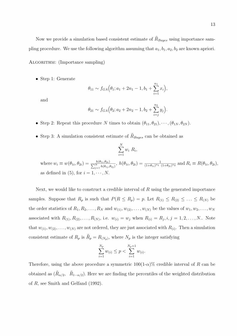
Now we provide a simulation based consistent estimate of RBayes using importance sam-

pling procedure. We use the following algorithm assuming that a1, b1, a2, b2 are known apriori.

Algorithm: (Importance sampling)

• Step 1: Generate

θ11 ∼ fGA

(θ1; a1 + 2n1 − 1, b1 +

n1∑i=1

xi

),

and

θ21 ∼ fGA

(θ2; a2 + 2n2 − 1, b2 +

n2∑i=j

yj).

• Step 2: Repeat this procedure N times to obtain (θ11, θ21), · · · , (θ1N , θ2N).

• Step 3: A simulation consistent estimate of RBayes can be obtained as

N∑i=1

wi Ri,

where wi ≡ w(θ1i, θ2i) =h(θ1i,θ2i)∑N

j=1h(θ1j ,θ2j)

, h(θ1i, θ2i) =1

(1+θ1i)n1 (1+θ2i)n2andRi ≡ R(θ1i, θ2i),

as defined in (5), for i = 1, · · · , N.

Next, we would like to construct a credible interval of R using the generated importance

samples. Suppose that Rp is such that P (R ≤ Rp) = p. Let R(1) ≤ R(2) ≤ . . . ≤ R(N) be

the order statistics of R1, R2, . . . , RN and w(1), w(2), . . . , w(N) be the values of w1, w2, . . . , wN

associated with R(1), R(2), . . . , R(N), i.e. w(i) = wj when R(i) = Rj, i, j = 1, 2, . . . , N.. Note

that w(1), w(2), . . . , w(N) are not ordered, they are just associated with R(i). Then a simulation

consistent estimate of Rp is Rp = R(Np), where Np is the integer satisfying

Np∑i=1

w(i) ≤ p <Np+1∑i=1

w(i).

Therefore, using the above procedure a symmetric 100(1-α)% credible interval of R can be

obtained as (Rα/2, R1−α/2). Here we are finding the percentiles of the weighted distribution

of R, see Smith and Gelfand (1992).

14

An alternative approach that replaces the importance sampling algorithm is to sample

directly from the joint posterior density of θ1 and θ2 using the acceptance-rejection method

as given by Smith and Gelfand (1992). This is mainly possible since in equations (13) and

(14), we have1

(1 + θ1)n1≤ 1 and

1

(1 + θ2)n2≤ 1 which imply that

l(θ1|data) ≤ c1 fGA

(θ1; a1 + 2n1 − 1, b1 +

n1∑i=1

xi

),

and

l(θ2|data) ≤ c2 fGA

(θ2; a2 + 2n2 − 1, b2 +

n2∑i=1

yi).

Once the posterior samples have been obtained, the Bayes estimate RBayes of R = (θ1, θ2),

as defined by (5), and the associated credible interval can be easily constructed. It may be

mentioned that for small values of n1 and n2, the acceptance rejection method can be very

effective in this case. On the other hand, for very large values of n1 and n2 this method can

be very inefficient, since in that case the proportion of rejection will be very large. Note that

once we generate samples directly from the joint posterior distribution, it is quite simple to

compute simulation consistent Bayes estimate with respect to other loss function also. For

example, if we want to compute the Bayes estimate under the absolute error loss function, i.e.

the posterior median, RBayes, it can be easily obtained from the generated samples obtained

from the posterior distribution. Detailed comparisons of the different Bayes estimators have

been presented in Section 5.

5. Simulation results

In this section we perform some simulation experiments to see the behavior of the proposed

methods for various sample sizes and for different sets of parameter values. We have taken

sample sizes namely (n1, n2) = (15, 20), (20, 15), (20, 20), (25, 30), (30, 25), (30, 30) and

two different sets of parameter values namely; (θ1, θ2) = (1.0, 1.0) and (0.1, 1.0), so that the

15

true reliability parameter values are 0.5 and 0.972, respectively.

For each pair of (n1, n2), we have generated samples from Lindley (θ1) and Lindley (θ2)

accompanied with B = 5000 bootstrap samples over 10,000 replications. Then, we report

for all sample sizes (a) the average bias and mean squared error of UMVUE and MLE (in

the logit scale), parametric bootstrap (Boots), and (b) the coverage probability (average

confidence length) of the simulated confidence intervals of R = P (Y < X) for different

values of θ1 and θ2. The calculations of those quantities in (a) and (b) above are given in

Tables 1, 2, 6, and 7.

For Bayes estimates we have taken different hyper-parameters of the priors, namely:

Prior-1: a1 = b1 = a2 = b2 = 0.0,

Prior-2: a1 = 4.0, b1 = 8.0, a2 = b2 = 4.0,

Prior-3: a1 = b1 = a2 = b2 = 4.0.

While Prior-1 is a non-informative prior, Prior-2 and Prior-3 are informative priors. We

have used both the algorithms mentioned in Section 4 to generate posterior samples, and

we denote them as Bayes-1 and Bayes-2, respectively. In computing the Bayes estimate

and the associated credible interval we have used N = 5000 importance sampling. In this

case also, we have computed the average biases and the mean squared errors of the Bayes

estimates and for the credible intervals we have computed the coverage percentages and

average lengths of the simulated intervals of R over 10,000 replications. For comparison

purposes, we have considered two different loss functions, namely squared error and absolute

error loss functions. The Bayesian simulation results are reported in Tables 3, 4, 5, 8, 9, and

10.

Some of the points are quite clear from the simulation results. For all the methods, as

the sample size increases the biases and the mean squared errors decrease. It verifies the

16

consistency properties of all the methods. Comparing the results from Tables 1 and 6, it

is observed that even for very small sample sizes the biases for all the estimators are quite

small and the absolute value of the bias of RUMV UE is much smaller than RMLE and RBoot.

The bias of RUMV UE seems not large enough even for small sample sizes. Indeed, Table 1

(Table 6) shows that discrepancies among the biases of the RUMV UE are in the fourth (fifth)

decimal places for all sample sizes.

RUMV UE is of course, unbiased by construction, and the very small biases that do show

up are the consequence of round off and finite number of iterations. This observation was

reported in Awad and Gharraf (1986) and Reiser and Guttman (1987) in the context of the

UMVUE of R in the Burr XII and normal cases, respectively.

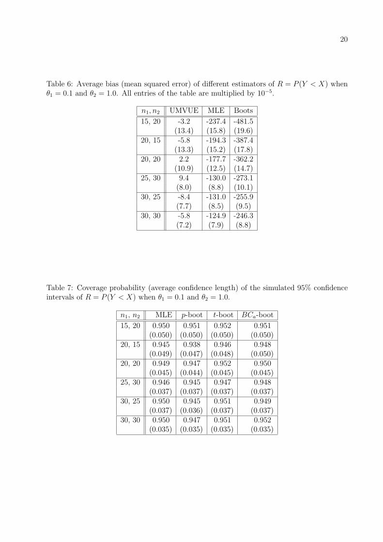
Now, we compare the MSE of R using UMVUE, MLE and parametric bootstrapping.

From Table 1, where R = 0.5, we observe that

MSE(RUMV UE) > MSE(RMLE) > MSE(RBoot).

From Table 6, where R = 0.972, we observe that

MSE(RUMV UE) < MSE(RMLE) < MSE(RBoot).

Reiser and Guttman (1987) reported similar simulation results for estimatingR using UMVUE

and MLE in the normal case.

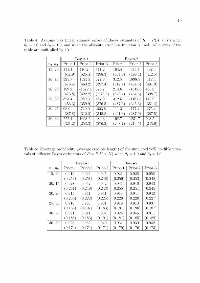
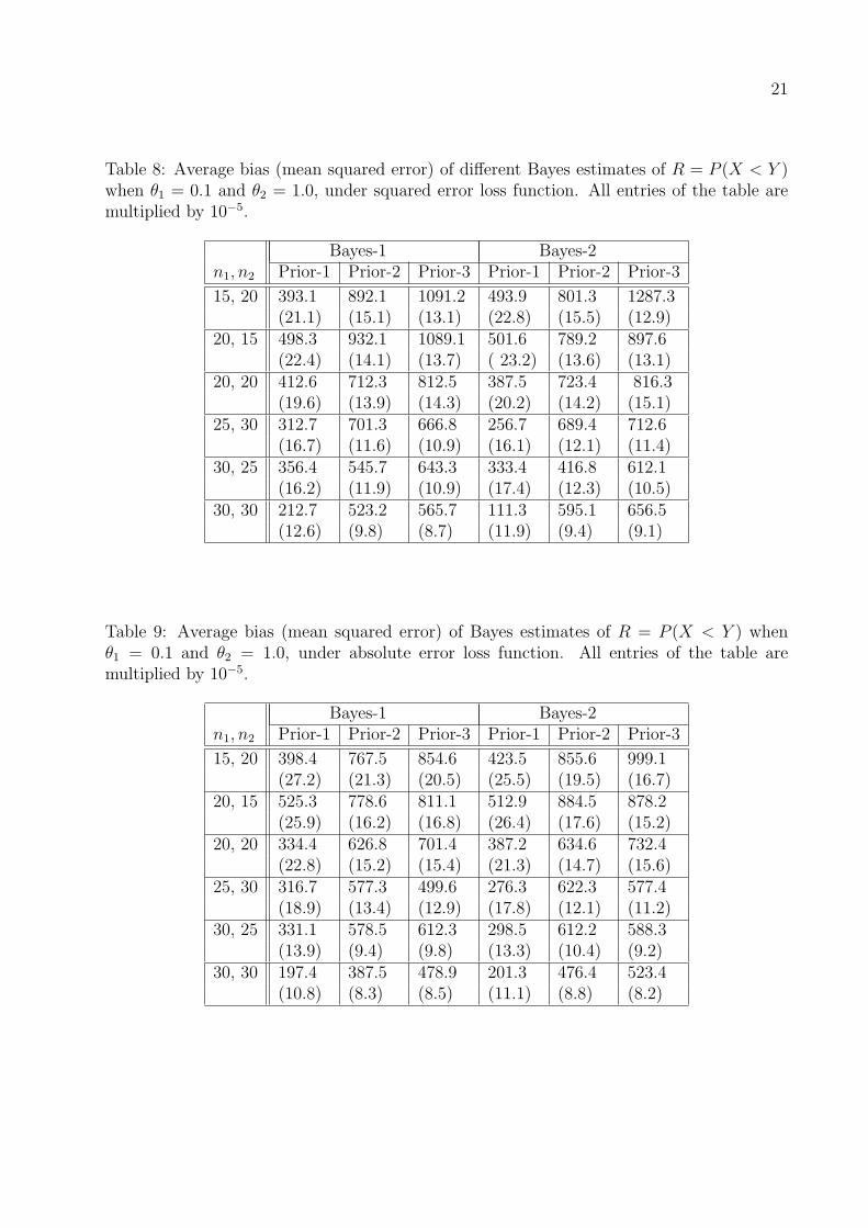
From the Tables 3, 4, 8, and 9, it is clear that both the Bayes estimators (Bayes-1 and

Bayes-2) behave quite similarly for each of the square and absolute error loss functions. As

expected, in most of the cases, it is observed that the Bayes estimators for Prior 2 or Prior 3

have a lower mean squared errors than the Bayes estimators obtained under Prior 1. Since

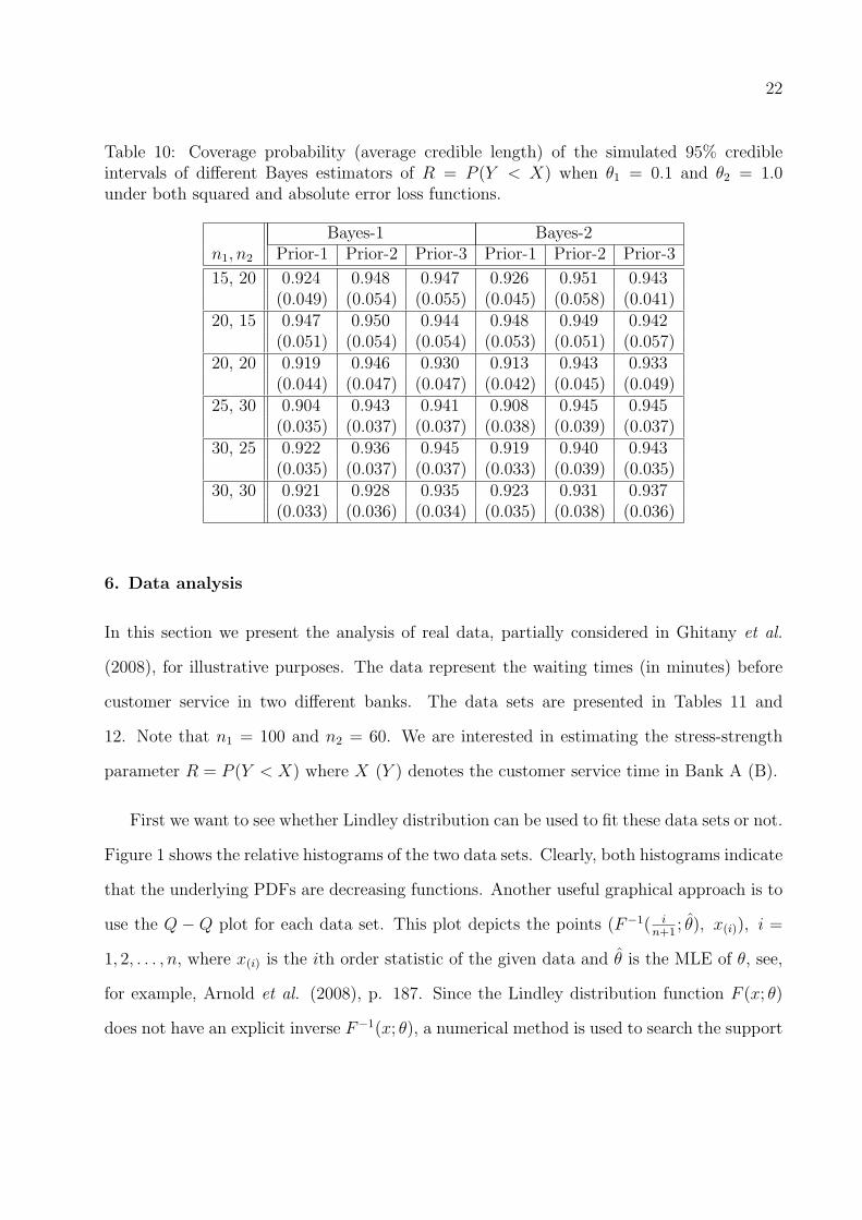
the credible intervals of R are based on its posterior distribution, the coverage probability

and average credible length do not depend on the error loss function used.

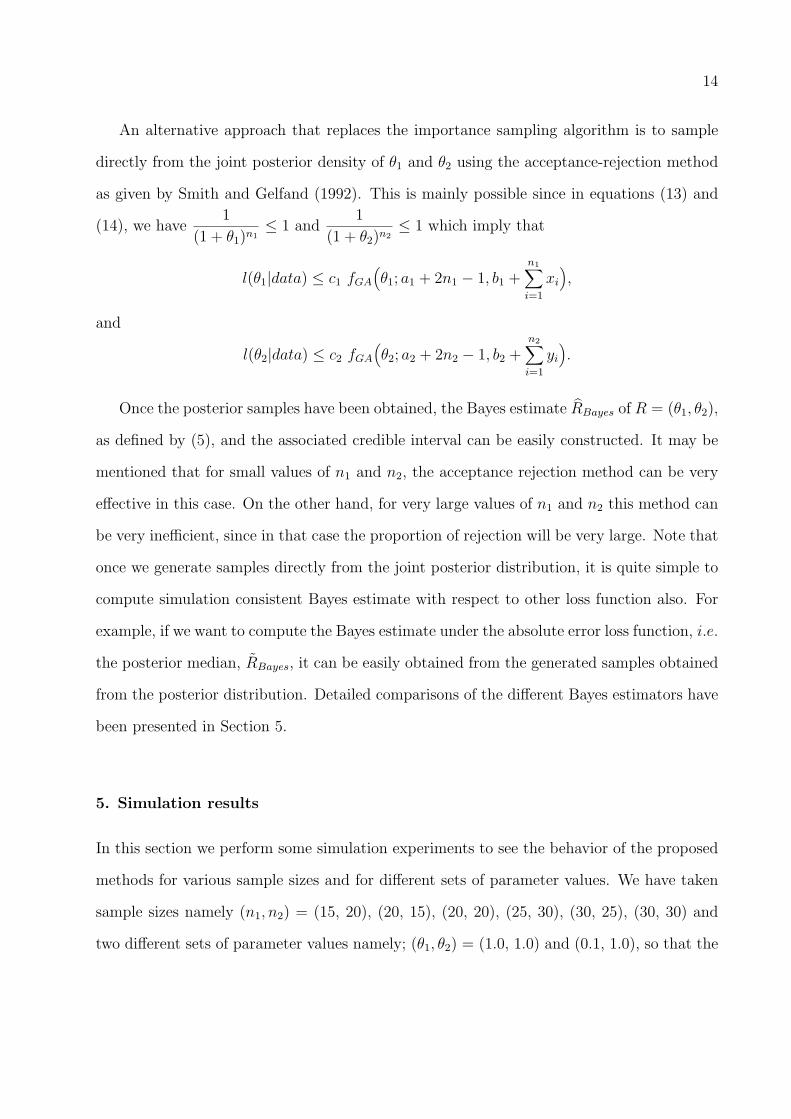
17

Table 1: Average bias (mean squared error) of different estimators of R = P (Y < X) whenθ1 = 1.0 and θ2 = 1.0. All entries of the table are multiplied by 10−5.

n1, n2 UMVUE MLE Boots

15, 20 54.4 -114.8 -274.8(806.2) (764.2) (727.9)

20, 15 -51.5 117.7 278.9(786.5) (745.6) (710.2)

20, 20 -13.4 -13.2 -13.9(697.4) (666.1) (637.9)

25, 30 19.6 -48.4 -114.5(496.9) (480.4) (465.4)

30, 25 -15.6 52.4 118.1(506.6) (489.8) (474.2)

30, 30 20.5 20.3 21.0(453.8) (440.1) (427.2)

The performances of the MLEs are very similar with the corresponding Bayes estimators

when the non-informative prior is used, and for both the loss functions used here. Interest-

ingly when the prior means are exactly equal to the true means, then the performances of

the Bayes estimators are slightly better than the MLEs, otherwise they are usually worse.

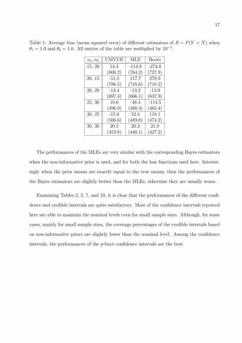
Examining Tables 2, 5, 7, and 10, it is clear that the performances of the different confi-

dence and credible intervals are quite satisfactory. Most of the confidence intervals reported

here are able to maintain the nominal levels even for small sample sizes. Although, for some

cases, mainly for small sample sizes, the coverage percentages of the credible intervals based

on non-informative priors are slightly lower than the nominal level. Among the confidence

intervals, the performances of the p-boot confidence intervals are the best.

18

Table 2: Coverage probability (average confidence length) of the simulated 95% confidenceintervals of R = P (Y < X) when θ1 = 1.0 and θ2 = 1.0.

n1, n2 MLE p-boot t-boot BCa-boot

15, 20 0.950 0.957 0.950 0.952(0.326) (0.337) (0.331) (0.331)

20, 15 0.950 0.948 0.950 0.951(0.326) (0.325) (0.331) (0.332)

20, 20 0.948 0.951 0.949 0.949(0.304) (0.308) (0.308) (0.309)

25, 30 0.948 0.952 0.949 0.948(0.265) (0.270) (0.267) (0.267)

30, 25 0.950 0.950 0.950 0.950(0.264) (0.265) (0.267) (0.267)

30, 30 0.947 0.949 0.948 0.947(0.253) (0.255) (0.255) (0.256)

Table 3: Average bias (mean squared error) of different Bayes estimates of R = P (X < Y )when θ1 = 1.0 and θ2 = 1.0. The loss function is squared error loss function. All entries ofthe table are multiplied by 10−5.

Bayes-1 Bayes-2n1, n2 Prior-1 Prior-2 Prior-3 Prior-1 Prior-2 Prior-3

15, 20 112.4 398.2 501.5 145.6 365.1 576.2(573.1) (511.1) (387.4) (512.5) 513.9 (394.5)

20, 15 331.8 -2318.3 392.5 298.6 -1873.5 367.8(498.5) (456.6) (398.7) (476.5) (298.5) (401.1)

20, 20 127.7 -2483.6 318.3 106 - 2674.3 402.5(499.3) (398.6) (278.6) (499.4) (401.3) (411.3)

25, 30 364.3 -2198.1 151.2 293.4 -2289.3 111.6(432.6) (299.3) (298.3) (451.2) (345.2) (401.4)

30, 25 192.5 -167.3 197.5 198.5 -156.7 149.2(398.6) (298.4) (305.3) (406.4) (265.2) (293.4)

30, 30 311.3 -1798.3 143.8 301.4 - 1789.3 131.2(321.8) (292.3) (287.5) (267.8) (298.1) (287.9)

19

Table 4: Average bias (mean squared error) of Bayes estimates of R = P (X < Y ) whenθ1 = 1.0 and θ2 = 1.0, and when the absolute error loss function is used. All entries of thetable are multiplied by 10−5.

Bayes-1 Bayes-2n1, n2 Prior-1 Prior-2 Prior-3 Prior-1 Prior-2 Prior-3

15, 20 111.4 410.2 511.2 104.4 375.4 487.4(641.9) (525.4) (398.3) (664.3) (499.4) (412.5)

20, 15 325.7 1323.2 377.8 312.5 1898.5 412.4(476.4) (463.2) (397.4) (512.4) (454.3) (401.9)

20, 20 189.2 -1672.4 376.7 214.6 -1512.8 435.6(476.8) (422.2) ( 376.3) (525.4) (434.6) (398.7)

25, 30 323.4 -989.3 187.9 312.5 -1167.5 112.9(456.3) (359.9) (376.5) (487.6) (345.6) (351.4)

30, 25 98.9 -749.9 -303.8 111.3 -777.4 -275.4(387.8) (312.2) (345.8) (401.3) (287.9) (367.5)

30, 30 222.4 1098.2 289.3 198.7 1231.7 268.5(321.2) (253.3) (276.3) (298.7) (214.5) (245.6)

Table 5: Coverage probability (average credible length) of the simulated 95% credible inter-vals of different Bayes estimators of R = P (Y < X) when θ1 = 1.0 and θ2 = 1.0.

Bayes-1 Bayes-2n1, n2 Prior-1 Prior-2 Prior-3 Prior-1 Prior-2 Prior-3

15, 20 0.919 0.923 0.945 0.921 0.926 0.958(0.253) (0.251) (0.246) (0.256) (0.253) (0.248)

20, 15 0.928 0.942 0.942 0.931 0.946 0.943(0.251) (0.249) (0.243) (0.255) (0.251) (0.245)

20, 20 0.915 0.941 0.941 0.918 0.944 0.942(0.230) (0.223) (0.225) (0.228) (0.220) (0.227)

25, 30 0.916 0.936 0.931 0.919 0.913 0.937(0.186) (0.197) (0.183) (0.191) (0.190) (0.187)

30, 25 0.921 0.941 0.904 0.928 0.946 0.911(0.185) (0.183) (0.191) (0.181) (0.185) (0.189)

30, 30 0.928 0.932 0.940 0.931 0.939 0.942(0.174) (0.174) (0.171) (0.179) (0.176) (0.173)

20

Table 6: Average bias (mean squared error) of different estimators of R = P (Y < X) whenθ1 = 0.1 and θ2 = 1.0. All entries of the table are multiplied by 10−5.

n1, n2 UMVUE MLE Boots

15, 20 -3.2 -237.4 -481.5(13.4) (15.8) (19.6)

20, 15 -5.8 -194.3 -387.4(13.3) (15.2) (17.8)

20, 20 2.2 -177.7 -362.2(10.9) (12.5) (14.7)

25, 30 9.4 -130.0 -273.1(8.0) (8.8) (10.1)

30, 25 -8.4 -131.0 -255.9(7.7) (8.5) (9.5)

30, 30 -5.8 -124.9 -246.3(7.2) (7.9) (8.8)

Table 7: Coverage probability (average confidence length) of the simulated 95% confidenceintervals of R = P (Y < X) when θ1 = 0.1 and θ2 = 1.0.

n1, n2 MLE p-boot t-boot BCa-boot

15, 20 0.950 0.951 0.952 0.951(0.050) (0.050) (0.050) (0.050)

20, 15 0.945 0.938 0.946 0.948(0.049) (0.047) (0.048) (0.050)

20, 20 0.949 0.947 0.952 0.950(0.045) (0.044) (0.045) (0.045)

25, 30 0.946 0.945 0.947 0.948(0.037) (0.037) (0.037) (0.037)

30, 25 0.950 0.945 0.951 0.949(0.037) (0.036) (0.037) (0.037)

30, 30 0.950 0.947 0.951 0.952(0.035) (0.035) (0.035) (0.035)

21

Table 8: Average bias (mean squared error) of different Bayes estimates of R = P (X < Y )when θ1 = 0.1 and θ2 = 1.0, under squared error loss function. All entries of the table aremultiplied by 10−5.

Bayes-1 Bayes-2n1, n2 Prior-1 Prior-2 Prior-3 Prior-1 Prior-2 Prior-3

15, 20 393.1 892.1 1091.2 493.9 801.3 1287.3(21.1) (15.1) (13.1) (22.8) (15.5) (12.9)

20, 15 498.3 932.1 1089.1 501.6 789.2 897.6(22.4) (14.1) (13.7) ( 23.2) (13.6) (13.1)

20, 20 412.6 712.3 812.5 387.5 723.4 816.3(19.6) (13.9) (14.3) (20.2) (14.2) (15.1)

25, 30 312.7 701.3 666.8 256.7 689.4 712.6(16.7) (11.6) (10.9) (16.1) (12.1) (11.4)

30, 25 356.4 545.7 643.3 333.4 416.8 612.1(16.2) (11.9) (10.9) (17.4) (12.3) (10.5)

30, 30 212.7 523.2 565.7 111.3 595.1 656.5(12.6) (9.8) (8.7) (11.9) (9.4) (9.1)

Table 9: Average bias (mean squared error) of Bayes estimates of R = P (X < Y ) whenθ1 = 0.1 and θ2 = 1.0, under absolute error loss function. All entries of the table aremultiplied by 10−5.

Bayes-1 Bayes-2n1, n2 Prior-1 Prior-2 Prior-3 Prior-1 Prior-2 Prior-3

15, 20 398.4 767.5 854.6 423.5 855.6 999.1(27.2) (21.3) (20.5) (25.5) (19.5) (16.7)

20, 15 525.3 778.6 811.1 512.9 884.5 878.2(25.9) (16.2) (16.8) (26.4) (17.6) (15.2)

20, 20 334.4 626.8 701.4 387.2 634.6 732.4(22.8) (15.2) (15.4) (21.3) (14.7) (15.6)

25, 30 316.7 577.3 499.6 276.3 622.3 577.4(18.9) (13.4) (12.9) (17.8) (12.1) (11.2)

30, 25 331.1 578.5 612.3 298.5 612.2 588.3(13.9) (9.4) (9.8) (13.3) (10.4) (9.2)

30, 30 197.4 387.5 478.9 201.3 476.4 523.4(10.8) (8.3) (8.5) (11.1) (8.8) (8.2)

22

Table 10: Coverage probability (average credible length) of the simulated 95% credibleintervals of different Bayes estimators of R = P (Y < X) when θ1 = 0.1 and θ2 = 1.0under both squared and absolute error loss functions.

Bayes-1 Bayes-2n1, n2 Prior-1 Prior-2 Prior-3 Prior-1 Prior-2 Prior-3

15, 20 0.924 0.948 0.947 0.926 0.951 0.943(0.049) (0.054) (0.055) (0.045) (0.058) (0.041)

20, 15 0.947 0.950 0.944 0.948 0.949 0.942(0.051) (0.054) (0.054) (0.053) (0.051) (0.057)

20, 20 0.919 0.946 0.930 0.913 0.943 0.933(0.044) (0.047) (0.047) (0.042) (0.045) (0.049)

25, 30 0.904 0.943 0.941 0.908 0.945 0.945(0.035) (0.037) (0.037) (0.038) (0.039) (0.037)

30, 25 0.922 0.936 0.945 0.919 0.940 0.943(0.035) (0.037) (0.037) (0.033) (0.039) (0.035)

30, 30 0.921 0.928 0.935 0.923 0.931 0.937(0.033) (0.036) (0.034) (0.035) (0.038) (0.036)

6. Data analysis

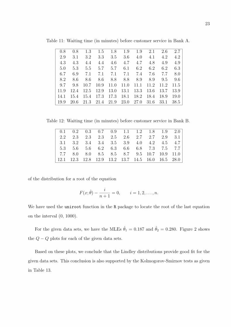
In this section we present the analysis of real data, partially considered in Ghitany et al.

(2008), for illustrative purposes. The data represent the waiting times (in minutes) before

customer service in two different banks. The data sets are presented in Tables 11 and

12. Note that n1 = 100 and n2 = 60. We are interested in estimating the stress-strength

parameter R = P (Y < X) where X (Y ) denotes the customer service time in Bank A (B).

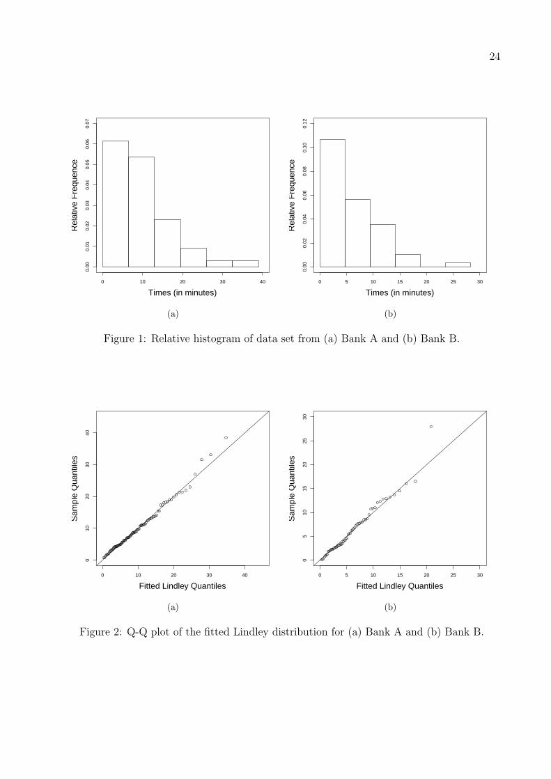
First we want to see whether Lindley distribution can be used to fit these data sets or not.

Figure 1 shows the relative histograms of the two data sets. Clearly, both histograms indicate

that the underlying PDFs are decreasing functions. Another useful graphical approach is to

use the Q − Q plot for each data set. This plot depicts the points (F−1( in+1

; θ), x(i)), i =

1, 2, . . . , n, where x(i) is the ith order statistic of the given data and θ is the MLE of θ, see,

for example, Arnold et al. (2008), p. 187. Since the Lindley distribution function F (x; θ)

does not have an explicit inverse F−1(x; θ), a numerical method is used to search the support

23

Table 11: Waiting time (in minutes) before customer service in Bank A.

0.8 0.8 1.3 1.5 1.8 1.9 1.9 2.1 2.6 2.72.9 3.1 3.2 3.3 3.5 3.6 4.0 4.1 4.2 4.24.3 4.3 4.4 4.4 4.6 4.7 4.7 4.8 4.9 4.95.0 5.3 5.5 5.7 5.7 6.1 6.2 6.2 6.2 6.36.7 6.9 7.1 7.1 7.1 7.1 7.4 7.6 7.7 8.08.2 8.6 8.6 8.6 8.8 8.8 8.9 8.9 9.5 9.69.7 9.8 10.7 10.9 11.0 11.0 11.1 11.2 11.2 11.511.9 12.4 12.5 12.9 13.0 13.1 13.3 13.6 13.7 13.914.1 15.4 15.4 17.3 17.3 18.1 18.2 18.4 18.9 19.019.9 20.6 21.3 21.4 21.9 23.0 27.0 31.6 33.1 38.5

Table 12: Waiting time (in minutes) before customer service in Bank B.

0.1 0.2 0.3 0.7 0.9 1.1 1.2 1.8 1.9 2.02.2 2.3 2.3 2.3 2.5 2.6 2.7 2.7 2.9 3.13.1 3.2 3.4 3.4 3.5 3.9 4.0 4.2 4.5 4.75.3 5.6 5.6 6.2 6.3 6.6 6.8 7.3 7.5 7.77.7 8.0 8.0 8.5 8.5 8.7 9.5 10.7 10.9 11.012.1 12.3 12.8 12.9 13.2 13.7 14.5 16.0 16.5 28.0

of the distribution for a root of the equation

F (x; θ)− i

n+ 1= 0, i = 1, 2, . . . , n.

We have used the uniroot function in the R package to locate the root of the last equation

on the interval (0, 1000).

For the given data sets, we have the MLEs θ1 = 0.187 and θ2 = 0.280. Figure 2 shows

the Q−Q plots for each of the given data sets.

Based on these plots, we conclude that the Lindley distributions provide good fit for the

given data sets. This conclusion is also supported by the Kolmogorov-Smirnov tests as given

in Table 13.

24

Times (in minutes)

Rel

ativ

e F

requ

ence

0 10 20 30 40

0.00

0.01

0.02

0.03

0.04

0.05

0.06

0.07

(a)

Times (in minutes)R

elat

ive

Fre

quen

ce0 5 10 15 20 25 30

0.00

0.02

0.04

0.06

0.08

0.10

0.12

(b)

Figure 1: Relative histogram of data set from (a) Bank A and (b) Bank B.

0 10 20 30 40

010

2030

40

Fitted Lindley Quantiles

Sam

ple

Qua

ntile

s

(a)

0 5 10 15 20 25 30

05

1015

2025

30

Fitted Lindley Quantiles

Sam

ple

Qua

ntile

s

(b)

Figure 2: Q-Q plot of the fitted Lindley distribution for (a) Bank A and (b) Bank B.

25

Table 13: Kolmogorov-Smirnov distances and the associated p−values.

Data set K-S statistic p-value

Bank A 0.068 0.750Bank B 0.080 0.840

Now we compute the UMVUE, MLE and Bayes estimates of R. Since we do not have any

prior information, we have used non-informative prior only. For the given data, RUMV UE =

0.647, RMLE = 0.645, Bayes-1 estimate of R is 0.631 under the squared error loss function

(0.637 under the absolute error loss function), and Bayes-2 estimate of R is 0.629 under the

squared error loss function (0.633 under the absolute error loss function).

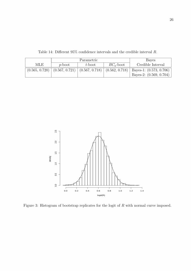
Different 95% confidence intervals and the credible interval of R based on logit trans-

formation are provided in Table 14. It is quite interesting to see that all the intervals are

virtually indistinguishable. To explore an explanation for this observation, we provide the

histogram of the bootstrap replicates for the logit of R based on B=5000 in Figure 3. Clearly,

the histogram resembles that of a normal distribution with approximate mean 0.6031 and

standard deviation 0.1752. A formally K-S test yields distance statistic 0.009 and p-value

= 0.854, confirming the normality of the bootstrap replicates for the logit of R. This can

be the reason that the confidence and credible intervals are almost indistinguishable for the

given data.

It is clear that the MLE and Bayes estimator with respect to non-informative prior

behave quite similarly, although the length of the credible interval is slightly shorter than

the corresponding confidence intervals obtained by different methods.

26

Table 14: Different 95% confidence intervals and the credible interval R.

Parametric BayesMLE p-boot t-boot BCa-boot Credible Interval

(0.565, 0.720) (0.567, 0.721) (0.567, 0.718) (0.562, 0.718) Bayes-1: (0.573, 0.706)Bayes-2: (0.569, 0.704)

0.0 0.2 0.4 0.6 0.8 1.0 1.2 1.4

0.0

0.5

1.0

1.5

2.0

2.5

logit(R)

dens

ity

Figure 3: Histogram of bootstrap replicates for the logit of R with normal curve imposed.

27

7. Conclusions

In this paper we have studied several point and interval estimation procedures of the stress-

strength parameter of the Lindley distribution. We have obtained the UMVUE of the stress-

strength parameter, however the exact or asymptotic distribution of it is very difficult to

obtain. We have derived the MLE of R and its asymptotic distribution. Also, different

parametric bootstrap confidence intervals are proposed and it is observed that the p-boot

estimate works the best even for small sample sizes.

We have computed the Bayes estimate of R based on the independent gamma priors and

using squared and absolute error loss functions. Since the Bayes estimate cannot be obtained

in explicit form, we have used the MCMC technique to compute the Bayes estimate and also

the associated credible interval. Simulation results suggest that the performance of the

Bayes estimator based on the non-informative prior works very well and it can be used for

all practical purposes.

Acknowledgements

The authors would like to thank the Associate editor and the reviewer for their helpful

comments which improved an earlier draft of the manuscript. The first author would like

to thank Kuwait Foundation for the Advancement of Sciences (KFAS) for financial support.

Part of the work of the third author has been supported by a grant from the Department of

Science and Technology, Government of India.

References

Arnold,B. C., Balakrishnan, N. and Nagaraja, H. N. (2008). A First Course in Order

Statistics. Philadelphia: SIAM.

28

Awad, A.M., Gharraf, M.K. (1986). Estimation of P (Y < X) in the Burr case: A compara-

tive study. Communications in Statistics-Simulation 15:389–403.

Birnbaum, Z.W. (1956). On a use of the Mann-Whitney statistic. In: Proceedings of Third

Berkeley Symposium on Mathematical Statistics and Probability, vol. 1, pp. 13–17, Univer-

sity of California Press, Berkeley, CA.

Birnbaum, Z.W., McCarty, R.C. (1958). A distribution-free upper confidence bound for

P{Y < X}, based on independent samples of X and Y . Annals of Mathematical Statistics

29:558–562.

Church, J.D., Harris, B. (1970). The estimation of reliability from stress-strength relation-

ships. Technometrics 12:49–54.

Efron, B., Tibshirani, R.J. (1998). An Introduction to Bootstrap. New York: Chapman &

Hall.

Ghitany, M.E., Atieh, B., Nadarajah, S. (2008). Lindley distribution and its application,

Mathematics and Computers in Simulation 78:493–506.

Kotz, S., Lumelskii, Y., Pensky, M. (2003). The Stress-Strength Model and its Generaliza-

tions: Theory and Applications. Singapore: World Scientific Press.

Krishnamoorthy, K., Mukherjee, S., Guo, H. (2007). Inference on reliability in two-parameter

exponential stress-strength model. Metrika 65:261–273.

Kundu, D., Raqab, M.Z. (2009). Estimation of R = P (Y < X) for three-parameter Weibull

distribution. Statistics and Probability Letters 79:1839–1846.

Kundu, D., Gupta, R.D. (2006). Estimation of R = P [Y < X] for Weibull distributions.

IEEE Transactions on Reliability 55:270–280.

29

Kundu, D., Gupta, R.D. (2005). Estimation of P [Y < X] for generalized exponential distri-

bution. Metrika 61:291–308.

Lindley, D.V. (1958). Fudicial distributions and Bayes’ theorem. Journal of the Royal

Statistical Society B 20:102–107.

Raqab, M.Z., Kundu, D. (2005). Comparison of different estimators of P [Y < X] for a

scaled Burr type X distribution. Communications in Statistics-Simulation and Computation

34:465–483.

Reiser, B., Guttman, I. (1987). A comparison of three different point estimators for P (Y <

X) in the normal case. Computational Statistics and Data Analysis 5:59–66.

Smith, A.F.M., Gelfand, A.E. (1992). Bayesian sampling without tears: a sampling-resampling

perspective. The American Statistician 46:84–88.