1 

Inference from ecological models: estimating the relative risk of stroke from air pollution exposure using small area data.

Robert Haining Department of Geography,

University of Cambridge, UK.

Guangquan Li Department of Epidemiology and Biostatistics,

Imperial College, London, UK.

Ravi Maheswaran Public Health GIS Unit, ScHARR,

University of Sheffield, UK.

Marta Blangiardo Department of Epidemiology and Biostatistics,

and MRC Centre for Environment and Health

Imperial College, London, UK.

Jane Law Department of Health Studies and Gerontology,

University of Waterloo, Canada

Nicky Best Department of Epidemiology and Biostatistics,

and MRC Centre for Environment and Health

Imperial College, London, UK.

Sylvia Richardson Department of Epidemiology and Biostatistics,

and MRC Centre for Environment and Health

Imperial College, London, UK.

Author for correspondence: R.Haining (rph26@cam.ac.uk)

  2 

Abstract:

Maheswaran et al. (2006) analysed the effect of outdoor modelled NOx levels, classified into quintiles, on stroke mortality using a Poisson Bayesian hierarchical model with spatial random effects. An association was observed between higher levels of NOx and stroke mortality at the small area (enumeration district) level.

As this model is framed in an ecological perspective, the relative risk estimates suffer from ecological bias. In this paper we use a different model specification based on Jackson et al. (2008), modelling the number of cases of mortality due to stroke as a binomial random variable where p(i) is the probability of dying from stroke in area i. The within-area variation in outdoor modelled NOx levels is used to determine the proportion of the population in area i falling into each of the five exposure categories in order to estimate the probability of an individual dying from stroke given the kth level of NOx exposure assuming a homogeneous effect across the study region. The inclusion of within area variability in an ecological regression model has been demonstrated to help reduce the ecological bias (Jackson et al., 2005, 2008). Revised estimates of relative risk are obtained and compared with previous estimates.

Key words: ecological bias; random effects; relative risk estimation; binomial regression; poisson regression

  3 

1. Introduction

Small area ecological studies are frequently undertaken to investigate associations between risk factors and health outcomes especially when the absolute number of cases of a disease is small. Where the effect of the risk factor is expected to be small, it may be difficult to attain standard levels of adequacy for the power of a test in a cohort study without a prohibitively large and possibly expensive sample. These circumstances often arise when attempting to assess an environmental risk factor in relation to health.

Small area ecological studies have certain advantages when studying the health impacts of exposure to air pollution. They provide an alternative way of looking at the risk-outcome relationship compared with, for example, studying severe pollution episodes where health outcomes will often reflect the harvesting of both acute and chronic cases. Small area studies also make it possible to study very large populations at a relatively low cost, compared to a cohort study. Although analyses of small area data may be affected by the small number problem, such areas are likely to be more homogeneous (than large areas) in terms of population characteristics thus reducing the risk of ecological bias (Gotway and Young, 2002). Also, analyses of populations, imputing to them air pollution exposure levels based on where they live, may be less affected by measurement error than analyses of individuals, imputing air pollution exposure levels from the same or similar data, since at the population level some of the individual level error might be expected to average out. For a review of methods of air pollution monitoring see for example Williams (1995) and for studies based on individual level data and estimates of air pollution exposure see for example Miller et al. (2007) and Jerrett et al. (2005).

Notwithstanding these remarks, the risk of aggregation or ecological bias underlies all ecological studies. As a consequence, whilst many epidemiologists may concede that small area level studies have a useful role to play in initial explorations of certain types of exposure-outcome relationships, relative risk estimates obtained from such studies are viewed with suspicion. They are population level estimates where the populations comprise unspecified levels of heterogeneity in terms of the other factors that may impact on health status. Treating such estimates as measures of risk at the individual level would represent an example of the ecological fallacy.

Whilst small area ecological studies continue to be used for analysing certain types of environmental exposure-health outcome relationships “statistical tools are needed to provide the best possible analyses under these circumstances, and the limitations of such analyses need to be fully documented” (Young et al. 2009, p.82).

Recently several approaches have been proposed to combine information from individual level and aggregated data, with the aim of correcting the ecological bias. Haneuse and Wakefield (2007, 2008) propose an approach that takes advantage of case-control individual level data to estimate a relationship between exposure and the outcome of interest. Their method evaluates the conditional distribution of aggregated data (what they call incomplete

  4 

data) given the individual level data (complete data), in a frequentist (Haneuse and Wakefield, 2007) or Bayesian framework (Haneuse and Wakefield, 2008).

Adopting a different perspective, Jackson et al. (2005, 2008) propose a methodology to combine aggregated and individual level data from epidemiological studies in a Bayesian hierarchical framework: the individual level data provide information on the true dose-response between exposure and outcome, correcting for the ecological bias which arises when the exposure is accounted for only at the aggregate level. They present several examples where small area exposure is combined with individual level covariates and outcomes. They specify two joint regression models in which the dose-response coefficient is assumed to be the same. The individual level data inform the coefficient and therefore correct the ecological bias.

The same principle can be followed when only covariates are available at the individual level and a binomial likelihood is assumed on the data. The proportion of individuals in each category is used as an estimate of the within-area distribution which corrects for the bias (see Jackson at al., 2008 for examples using three dichotomous covariates available at the individual level).

Maheswaran et al. (2006) analyse the effect of outdoor modelled NOx levels, classified into quintiles, on stroke mortality in Sheffield, England using a Poisson Bayesian hierarchical model with spatial random effects to model the small area counts and estimate the relative risk associated with increasing levels of NOx exposure. Stroke is the third most common cause of death in England and Wales and accounts for 9% of all deaths in men and 13% in women in the UK (http://www.stroke.org.uk/media_centre/facts_and_figures/index.html). Links to exposure to air pollution have generally been studied either focusing on severe pollution episodes such as the London smog of 1952 (Logan, 1953), or analysing daily time series such as Kan et al.’s (2003) study of Shanghai or cohort studies such as Nafstad et al.’s (2004) study of Norwegian males. In this paper we modify the modelling framework to take into account the within-area variation in exposure, following Jackson et al. (2008) and we specify a binomial Bayesian hierarchical model for the small area counts of stroke mortality. We then compare the results of the two modelling frameworks.

The paper is structured as follows: in the next section we briefly review the data sources used to explore the association between exposure to nitrogen oxides (NOx) and stroke mortality in Sheffield, England between 1994 and 1998; then we present the Bayesian model, followed by the results and concluding remarks.

2. Data Sources

The stroke mortality data is based on ICD9 codes 430-438. Between 1994 and 1998 there were approximately 3,000 deaths in Sheffield’s over 45 population of 200,000. Counts were aggregated by nine, 5 year age cohorts (from 45 to 85+), by sex and by enumeration districts (EDs) which comprise on average 150 households. There were approximately 2.89 deaths per ED and the minimum and maximum expected counts given the age-sex composition were 0.1 and 10.9 respectively.

  5 

The 1991 UK Census provided data on demography and deprivation for the n=1030 EDs. Population counts were corrected for under-enumeration at the Census and then scaled to the Sheffield Health Authority’s mid-year estimates for 1994-8. The Townsend index was used to measure material deprivation (Townsend et al. 1988). The index is a standardized combination of four Census variables measured as the percentage of households: with no car; where the head of household is unemployed; with more than one person per room; not owner occupied. The Townsend index calculated at the ED level was obtained from MIMAS (Manchester Information and Associated Services).

In the original study, data from the Sheffield Health and Illness Prevalence Survey in 2000 was used to provide a measure of smoking prevalence. However smoking prevalence was found not to be statistically significant and has been omitted from the present study. This was and remains a weakness in this study. For more information on the smoking prevalence data and possible reasons as to why it was not found to be significant in the earlier study see Maheswaran et al. (2006, p.503-4; 512-3).

Modelled NOx data were supplied by Sheffield City Council. The Indic Airviro model (SMHI Inc) provided these data taking as inputs data from point (e.g. factories), line (e.g. roads) and area (e.g. emissions from housing estates) sources of outdoor NOx. Information on photochemical processes and meteorological variables (temperature, radiation, wind speed and direction) was incorporated in the model. The NOx modelled values were output to a 200m grid square resolution for each of the years 1994-9 (excluding 1998 due to incomplete weather data) and then averaged.

Modelled NOx values were consistently higher than monitored values. Modelled values were rescaled to monitored equivalent values using linear regression. However absolute values of NOx and calculating relative risk in terms of unit increases in NOx were deemed unreliable so the data were converted to quintiles. This approach has the further advantage of avoiding assuming a linear relationship between NOx exposure and stroke mortality risk. For more detail on the construction of the NOx data values see Brindley et al. (2004).

Figure 1 shows a plot of ED level stroke mortality rates classified by NOx quintile. Within quintiles 4 and 5 there are some EDs with much higher stroke mortality rates and their presence raises the mean stroke mortality rate (red dots) for these two quintiles compared to quintiles 1-3. This provides some evidence of an association between higher rates of NOx exposure and higher stroke mortality rates but models are needed to assess this variability properly.

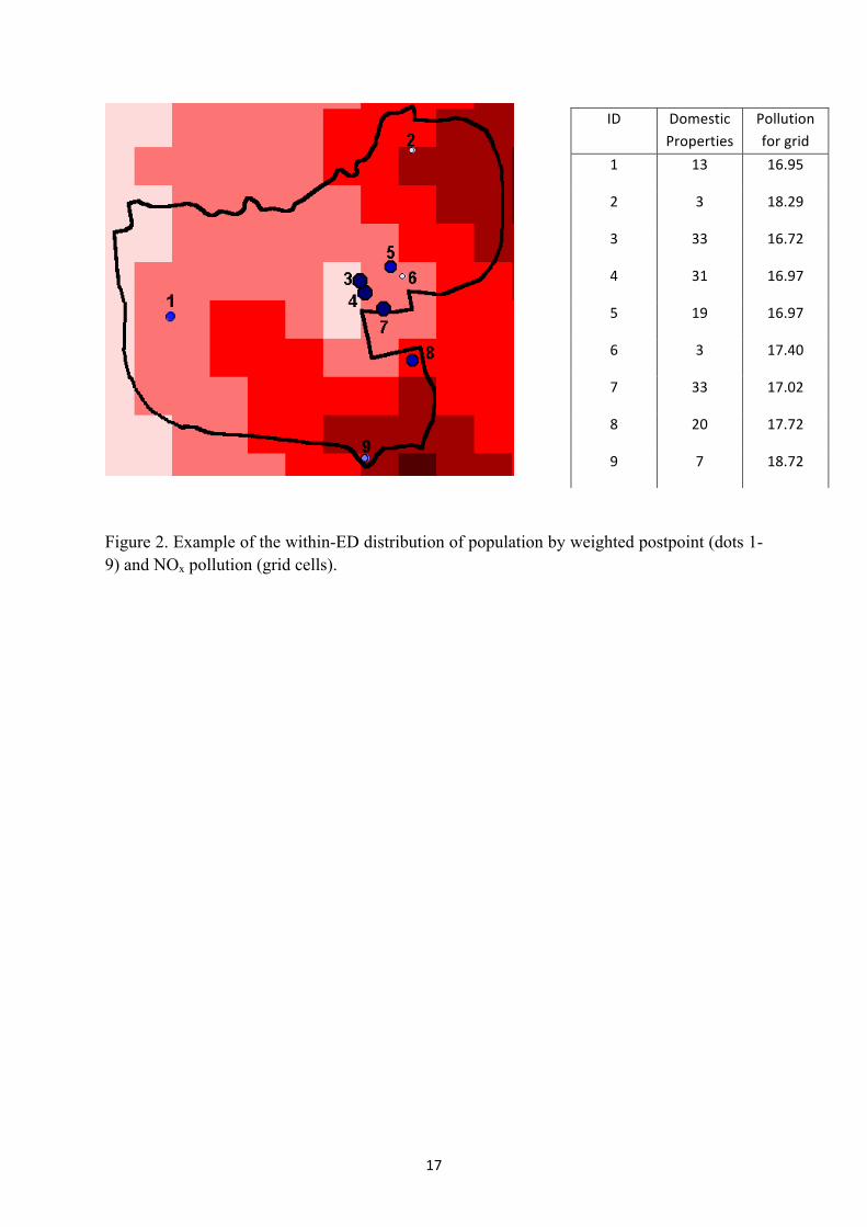
Figure 2 shows for one of Sheffield’s EDs the location and number of the domestic mail delivery points (postpoints) for each postcode superimposed on the scaled NOx values for 200m grid squares. In Maheswaran et al. (2006) each ED was assigned a single population weighted average NOx pollution value which was calculated as the product of the grid pollution value and the number of domestic properties attached to that cell, summing over all postpoints and then dividing by the number of domestic properties. For a description and assessment of this methodology see Brindley et al. (2005). In this study, however we retain

  6 

the information on the within-area distribution of NOx pollution and the within-area distribution of population in order to calculate the proportion of the population exposed to different (quintile) levels of pollution at the ED level.

The dataset was divided into five categories using quintiles of NOx, with an approximately equal number of EDs within each category. The same cut-off values were used to investigate the proportion of the population that fell into each NOx category within a CED and the cut-off values were the same as those used in previous work (Maheswaran et al 2006). Note that the variation of the within-area NOx exposure is quite small in the present data. 743 EDs (72% of a total 1030 EDs) have more than 70% of the population exposed to one of the 5 levels of NOx pollution. For a majority of the remaining 287 EDs the population is mainly distributed into two exposure levels; an example of the population distribution would be 0%, 8%, 56%, 36% and 0% for the first (the lowest exposure) level to the fifth (the highest exposure) level, respectively. There are only 23 (2%) EDs with a population somewhat equally spread across the 5 exposure levels.

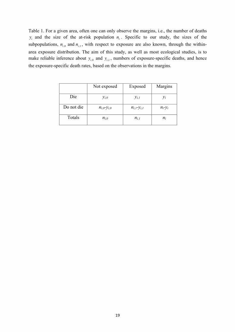
Table 1 illustrates the difference in the two approaches using a simple binary distinction (exposed or not exposed to air pollution). The variables yi and ni denote the total number of stroke deaths and the total population in the ith ED respectively – both were observed and were used in Maheswaran et al (2006). Of the other four variables, data for ni,0 and ni,1 were available (the within-ED count of the exposed and non-exposed population ) but not used. The variables yi,0 and yi,1 are unknown but are of interest.

3. Data Modelling and Analysis

To incorporate the within-area exposure information, we start with the underlying individual-level model and then aggregate up to the area-level. At the individual level, we have a binary outcome associated with an exposure variable for person in area . Let be the

stroke risk for this person and we have

. (1)

Using the logit link function, is modeled linearly by , an intercept, , an area-

specific age-sex adjusted fixed offset (see below), the effect of exposure and ,

effects contributed from other observed area-level covariates such as deprivation. We include a random effect term , which is a surrogate for other unmeasured, area-level risk factors and helps to explain a proportion of the random error unaccounted for by the exposure and other covariates. In this study, xi,j is the NOx exposure category for person j in area i (taking the lowest category as the reference level) and zi is the Townsend deprivation quintile, anchored at the first quintile (the most affluent group). The offsets, , were fixed to

where is the age-sex adjusted risk of stroke mortality calculated using indirect standardization with internal reference rates based on 18 age and sex strata. The

  7 

intercept, , is the (logit) risk, adjusted for age and sex, for the most affluent people in the city exposed to the lowest level of NOx pollution.

Since stroke is not contagious, independent Bernoulli random variables are aggregated to binomial random variables at the ED level. Therefore we have

(2)

where and are the observed stroke deaths and population at risk, respectively. The area-level stroke risk is given by the expectation of the individual-level risks

and the expectation is taken with respect to the exposure distribution in area ,

i.e.,

. (3)

The second equality is obtained by assuming that the exposure variable is categorized into levels so that is the proportion of people in the area who are exposed to NOx level

, representing the within-area exposure distribution. The exposure-specific risk, in area is obtained by replacing in Equation (1) by the effect of exposure at the

level, namely

(4)

where is the inverse of the logit function. We fitted the model defined by Equations (2-4) to two sets of data, one with two exposure categories and one with five exposure categories . In both cases, the first (lowest) level of exposure is set to be the reference group so and for is the odds ratio associated

with the level of exposure. For comparison, we also fitted a binomial model (with both unstructured and spatially structured random effects) where exposure was defined by the population-weighted average NOx level in each ED, categorized into quintiles. In this case, ecological bias is introduced as we wish to make inference at the individual level while the exposure is aggregated to the ED level. Figure 3 presents the Directed Acyclic graphs (DAG) for the above two models: (a) the binomial model incorporating the within-area exposure information and (b) the binomial model with an area-level categorical exposure. Circles represent unknown parameters (e.g., effects of exposure) whereas squares are observations (e.g., observed cases and covariates). Solid arrows denote stochastic dependence, while dashed arrows indicate functional relationship. In Model (a), the incorporation of the within-area exposure distribution allows the inference of stroke risk from the area-level ( ) down to the individual-level ( ). However, for Model (b) inference remains at the area-level.

To account for the uncertainty regarding the NOx measurements, we extend Equation (3) so that becomes a latent variable, representing the true proportions as if the NOx exposure could be measured without errors. Specifically, for each ED, we model the numbers of people

  8 

in each exposure category, , obtained by multiplying the observed proportions by the total number of people in that ED, by a multinomial distribution. That is,

. (5)

A vague Dirichlet prior, where (for data with 5 categories), is then assigned to the latent proportions. Prior distributions are required to complete the model specified in Equations (2)-(4). A Normal(0,10) is used for and a flat prior Normal(0,100) is used for the exposure effect and the coefficients associated with the Townsend index of deprivation. For the random effect term two priors are considered, namely a spatially

unstructured normal prior and a spatially structured prior

, where is the number of neighbours of area and

denotes a set of indicators of its neighbours. This is a typical representation of the intrinsic conditional autoregressive model (CAR) (Besag et al, 1991). A model without any random effect term and a model with both the unstructured and spatially structured random effects are also fitted. We have assessed the influence of the prior specification for the random effect variance by using two vague priors, a) a Gamma(0.5,0.005) on the precision and b) a uniform(0.01,1) on the standard deviation (Gelman 2006).

Inference for parameters of interest is drawn from the joint posterior density,

.

Since the above density is usually not analytically tractable, simulation-based methods are often employed for making posterior inference. The models described above have been implemented in WinBUGS (Lunn et al. 2000) and the code for a version of Model (a) is attached in Appendix 1. For each model, two chains with different starting values were run for 20,000 iterations with the first half discarded as burn-in (for the binomial model with no within-area distribution and with both types of random effects (one in column 3 of Table 4), 70,000 iterations with 60,000 burn-in were required for reasonable convergence). Convergence was checked using routine tools such as the trace plots and the Gelman-Rubin statistics (Gelman and Rubin, 1992 and Brooks and Gelman, 1997) provided in the software.

4. Results

The modelling in this paper utilises the information on within-area NOx exposure. Table 2 reports estimates of the relative risk from fitting four binomial models to data with 9x2 age-sex cohorts and either 2 or 5 exposure categories. Deprivation is controlled by using the Townsend index as an area-level covariate. Although different specifications for the random effects term were used, the first three models consistently show that high NOx levels are

  9 

associated with increased stroke mortality, after adjusting for the effects of age, sex and deprivation. Furthermore, incorporation of the uncertainty in the NOx measurements has little impact on this conclusion (last column of Table 2).

The estimation of the risks, however, is quite sensitive to the model specifications. When either only the unstructured or both the unstructured and spatially-structured random effects were included, the relative risks for categories 2-5 are all considerably reduced compared to those from the model without any random effects (Table 2). Similar estimates were obtained from fitting the models with the two types of random effects. Inclusion of the uncertainty in the NOx measurements, as formulated in Equation (5) yields estimates that are virtually identical to those in columns 4 and 5 but the credible intervals are slightly wider. We have performed a sensitivity analysis on how the relative risk estimates would be affected by the ways of constructing the exposure categories. More specifically, categories 4 and 5 are grouped as the exposed category while categories 1-3 are combined to form the non-exposed category. Estimated from the model with only the unstructured random effects and no measurement error component (Table 2), we obtained a slightly lower yet significant risk (1.18 and 95% CI 1.03 – 1.35) associated with people in the exposed category. The same conclusion can be drawn from the other three models but the risk estimate is again much higher for the model without random effects. It should be noted that we have experienced difficulties in fitting models with the measurement error component, in particular when including the spatially-structured random effects. Given that the uncertainty in exposure has little impact on the risk estimates, we will present results from models without this component.

We have investigated the performance of different types of models using the Deviance Information Criterion (DIC, Spiegelhalter et al. 2002) presented in Table 3. and

respectively measure the goodness of fit and the model complexity; a smaller value of DIC indicates a better fit of the model. The much larger DIC value from a model with no random effects suggests that it is necessary to account for unmeasured covariates in the analysis. Three types of random effects were examined, namely, (a) the unstructured random effects, (b) the spatially-structured random effects and (c) a combination of the unstructured and spatially-structured random effects. Comparing the three models, when fitted to data with either 2 or 5 exposure categories, (a) and (c) performed equally well and both are better than (b) (Table 3). From model (c), the estimated spatial fraction, measuring the percentage of variability explained by the spatially-structured random effects relative to the unstructured random effects, is small (0.013 with 95% CI 0.001 – 0.060). This indicates that the residual relative risks are dominated by the unstructured heterogeneity, consistent with the study by Maheswaran et al. (2006). Results in Table 4 are obtained from fitting two more sets of models in which we assigned each ED to one of the 5 exposure categories, defined by quintile. These models are similar to those fitted in Maheswaran et al. (2006) and are prone to ecological bias as the information on the within-area distribution is ignored. Besides the binomial distribution, we also considered the Poisson distribution as the sampling distribution. Two types of random effects

  10 

were used (specified in the column description of Table 4). Apart from the binomial model with both the unstructured and spatially structured random effects which clearly did not fit the data well (with a large DIC value) and also poor mixing, the risk estimates are virtually identical for the remaining three models (Table 4). Furthermore, for the binomial model with the unstructured random effects only, incorporation of the proportional information on exposure leads to moderate increments in risk for categories 2-4 (column 4 in Table 2), compared to those when the information was ignored (column 2 in Table 4). The risk for the highest exposure category, however, was reduced slightly. These changes are quantified in Table 5. In addition, comparable fits were obtained from the two sampling distributions, the binomial and Poisson models (DIC values in Table 4), indicating that the Poisson model is a reasonably good approximation to the binomial for this set of data.

The results reported here all use the Gamma(0.5,0.005) prior for the precision of the random effects. A uniform prior produced similar results (not shown).

5. Discussion and conclusions

The current approach uses within area information as a proxy for individual level information, i.e. the proportion of people exposed to different NOx categories in each ED, to reduce potential bias in the estimation of relative risk associated with environmental exposures that might be harmful to health. Using a more appropriate statistical framework, we are more confident in the finding that exposure to high levels of outdoor NOx is significantly associated with an elevated risk of stroke at the individual level.

Salway and Wakefield (2005, see also Wakefield and Salway, 2001) discuss that one of the sources of ecological bias comes when one ignores the within-area variability in its presence. The model applied here aims to reduce the bias by incorporating the within-area distribution of NOx exposure, which was not utilized in the previous study. It has been shown that for a continuous exposure, reduction of bias in parameter estimates can be achieved by including a small set of individual data, which facilitate the estimation of within-area variation (simulation cases 12-13 in Jackson et al. 2006). Here with a categorical exposure, information on the proportions of people exposed to different NOx categories is sufficient to provide this estimate (Jackson et al. 2008) and hence to improve the validity of individual-level inference. Although not substantial, differences in the risk estimates have been observed from comparing models with/without incorporation of the within-area exposure distribution. The changes are minor due to the small within-area variability present in the current dataset. For most EDs, the level of exposure across the population is quite homogeneous with the majority of people exposed to only one of the five NOx levels. Therefore, albeit prone to ecological bias, the models without consideration of the within-area exposure distribution (those presented in Table 4) can still provide somewhat reliable individual-level risk estimates. However, when sizable within-area variability in exposure is present, the individual-level inference from the above models becomes less accurate because of ecological bias and one should try to combine additional individual data (usually obtained from surveys and cohort studies) to strengthen the inference.

  11 

The model framework considered here is flexible to deal with many difficulties that arise from studies in environmental epidemiology. Different types of random effects can be used to account for unmeasured covariates, that if omitted can lead to less accurate inference (Salway and Wakefield 2005). In our study, if one were to conclude from results without accounting for the potential effects of unobserved covariates, the effect of NOx on stroke risks would be over-interpreted by an average of 10%. Being in a Bayesian framework, measurement errors (in exposure), inevitable in environmental epidemiology, can be easily dealt with (e.g., Richardson and Gilks, 1993). We have shown that the uncertainty in NOx measurements appears to have a minimal impact on the results but one should note that this additional modeling only allows for sampling variation in the NOx exposures, and that there may be more systematic misclassification that has not been accounted for.

The binomial distribution used in the present study has two additional advantages. Firstly, the binomial distribution is the true underlying sampling distribution for the present type of data, where the number of cases and the size of the population are available. The Poisson distribution, though commonly used, is only an approximation to the binomial. Secondly, we can express the area-level stroke risk as a weighted average of the exposure-specific risks (as in Equation 3) in the binomial setting as we are operating on probabilities. This operation, however, cannot be done on relative risks from a Poisson model, although Jackson et al (2006) do show how a Poisson version of the model with within-area exposures can be formulated for rare diseases.

For any Bayesian analysis, it is always a good practice to perform a sensitivity analysis on the impact from prior specification. Our conclusions are robust to the different priors we have considered.

Although cigarette smoking is a known risk factor for stroke, one of the findings from Maheswaran et al. (2006) is that smoking appears to have little effect on stroke mortality in the given data. Following their consideration, smoking was therefore not included in our analysis. Various methods have been proposed to use lung cancer mortality as a proxy for smoking (Peto et al. 1992; Ezzati and Lopez, 2003; and Best and Hansell, 2009). Problems related to the quality of the available smoking data (see Maheswaran et al. (2006)) could potentially be overcome. However, there is some evidence suggesting that exposure to air pollution increases lung cancer risk and adjustment based on lung cancer mortality might therefore inappropriately remove some of the excess stroke risk associated with air pollution (Vineis et al. 2004).

In conclusion, the finding that exposure to high levels of NOx significantly increases stroke mortality is robust, that is, it is not affected by ecological biases created as a result of ignorance about within-area exposure information and potential measurement errors. In addition, the current modeling framework should be used for quantifying the individual risks because it properly accounts for the within-area variability, potential effects of unobserved covariates and can be easily extended to deal with measurement errors.

Appendix 1.

  12 

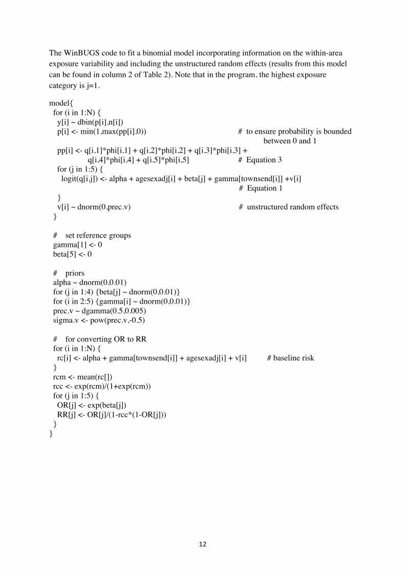
The WinBUGS code to fit a binomial model incorporating information on the within-area exposure variability and including the unstructured random effects (results from this model can be found in column 2 of Table 2). Note that in the program, the highest exposure category is j=1.

model{ for (i in 1:N) { y[i] ~ dbin(p[i],n[i]) p[i] <- min(1,max(pp[i],0)) # to ensure probability is bounded between 0 and 1 pp[i] <- q[i,1]*phi[i,1] + q[i,2]*phi[i,2] + q[i,3]*phi[i,3] + q[i,4]*phi[i,4] + q[i,5]*phi[i,5] # Equation 3 for (j in 1:5) { logit(q[i,j]) <- alpha + agesexadj[i] + beta[j] + gamma[townsend[i]] +v[i] # Equation 1 } v[i] ~ dnorm(0,prec.v) # unstructured random effects } # set reference groups gamma[1] <- 0 beta[5] <- 0 # priors alpha ~ dnorm(0,0.01) for (j in 1:4) {beta[j] ~ dnorm(0,0.01)} for (i in 2:5) {gamma[i] ~ dnorm(0,0.01)} prec.v ~ dgamma(0.5,0.005) sigma.v <- pow(prec.v,-0.5) # for converting OR to RR for (i in 1:N) { rc[i] <- alpha + gamma[townsend[i]] + agesexadj[i] + v[i] # baseline risk } rcm <- mean(rc[]) rcc <- exp(rcm)/(1+exp(rcm)) for (j in 1:5) { OR[j] <- exp(beta[j]) RR[j] <- OR[j]/(1-rcc*(1-OR[j])) } }

  13 

Acknowledgements

The work reported used data provided with the support of the ESRC and JISC, and census and boundary material and road vector data, which are copyright of the Crown, the Post Office, the ED-LINE Consortium, the Automobile Association and Ordnance Survey. Part of the study was funded by a grant from the Trent Research Scheme and part of the analysis was carried out by members of the Imperial College BIAS node of the ESRC National Centre for Research Methods (grant numbers RES-576-25-5003 and RES-576-25-0015). We would like to thank Sheffield City Council for providing the air pollution data.

The views expressed in this publication are those of the authors and not necessarily those of the funding organizations or data providers.

  14 

References Besag J, York J, Mollie A. Bayesian image restoration with two applications in spatial statistics. Ann. Inst. Stat. Math. 1991; 43: 1-59. Best N and Hansell AL. Geographic variations in risk: adjusting for unmeasured confounders through joint modeling of multiple diseases. Epidemiology 2009. 20:400-41 Brindley P, Maheswaran R, Pearson T, Wise S, Haining R. Using modeled outdoor air pollution data for health surveillance. In R.Maheswaran and M. Craglia (eds) GIS in Public Health Practice, Boca Raton, CRC Press, 2004, p.125-149. Brindley P, Wise SM, Maheswaran R, Haining R. The effect of alternative representations of population location on the areal interpolation of air pollution exposure. Computers, Environment and Urban Systems 2005; 29: 455-9.

Brooks, SP. and Gelman, A. General methods for monitoring convergence of iterative simulations, Journal of Computational and Graphical Statistics, 1997, 7:434–455.

Ezzati, M. and Lopez, AD. Estimates of Global Mortality Attributable to Smoking in 2000 Lancet 2003, 362 : 9387 847 – 52.

Gelman A. Prior distributions for variance parameters in hierarchical models. Bayesian Analysis 2006; 1(3): 515-533

Gelman, A. and Rubin, DB, Inference from iterative simulation using multiple sequences, Statistical Science, 1992, 7:457–472.

Gotway C.A. and Young L.J. Combining incompatible spatial data. Journal of the American Statistical Association 2002, 97(458): 632-648.

Haneuse S and Wakefield J. Hierarchical models for combining ecological and case-control data. Biometrics 2007; 63(1): 128-136

Haneuse S and Wakefield J. The combination of ecological and case-control data. Journal of the Royal Statistical Society, B 2008; 70(1): 73-93

Jackson, C., Best N. and Richardson, S. Improving ecological inference using individual-level data. Statistics in Medicine, 2005; 25, 2136-2159.

Jackson C, Best N and Richardson S. Hierarchical related regression for combining aggregate and individual data in studies of socio-economic disease risk factors. Journal of the Royal Statistical Society A 2008; 171(1): 159-178.

Jerrett M, Burnett RT, Ma RJ, Pope CA, Krewski D, Newbold KB, Thurston G, Shi YL, Finkelstein N, Callee EE, Thun MJ. Spatial analysis of air pollution and mortality in Los Angeles. Epidemiology 2005; 16 (6): 727-736.

  15 

Logan WPD. Mortality in the London fog incident, 1952. Lancet 1953; 1: 336-8.

Lunn, D.J., Thomas, A., Best, N., and Spiegelhalter, D. (2000) WinBUGS -- a Bayesian modelling framework: concepts, structure, and extensibility. Statistics and Computing, 10:325-337. Maheswaran R, Haining R, Pearson T, Law J, Brindley P, Best N. Outdoor NOx and stroke mortality: adjusting for small area level smoking prevalence using a Bayesian approach. Statistical Methods in Medical Research 2006; 15 (5): 499-516.

Miller KA, Siscovick DS, Sheppard L, Shepherd K, Sullivan JH, Anderson GL, Kaufman JD Long term exposure to air pollution and incidence of cardiovascular events in women. The New England Journal of Medicine 2007; 356 (5): 447-458.

Peto R., Lopez A.D., Boreham J., Thun M. and Heath Jr C. Mortality from tobacco in developed countries: indirect estimation from national vital statistics. Lancet 1992; 339:1268-78. Richardson S and Gilks WR. A Bayesian approach to measurement error problems in epidemiology using conditional independence models. International Journal of Epidemiology. 1993, 138(6): 430-442. Salway R. and Wakefield J. Sources of bias in ecological studies of non-rare events. Environmental and Ecological Statistics 2005; 12: 321-347.

Spiegelhalter, D. J., Best, N. G., Carlin, B. P., and Van der Linde, A. 2002. Bayesian Measures of Model Complexity and Fit (with discussion), Journal of the Royal Statistical Society, Series B, 64(4): 583-616.

Townsend P, Phillimore P, Beattie A. Health and deprivation: inequality and the North. London, Croom Helm, 1988.

Vineis P, Forastiere F, Hoek G, Lipsett M. Outdoor air pollution and lung cancer: recent epidemiologic evidence. International Journal of Cancer. 2004;111:647-52.

Wakefield, J. and Salway, R. A statistical framework for ecological and aggregate studies, Journal of the Royal Statistical Society, Series A; 164: 119-137.

Williams ML. Monitoring of exposure to air pollution. Science of the Total Environment 1995; 168 (2): 169-174. Young LJ, Gotway C, Yang J, Kearney G, DuClos C. Linking health and environmental data in geographical analysis: It’s so much more than centroids. Spatial and Spatio-Temporal Epidemiology, 2009; 1(1): 73-84

  16 

Figure 1. ED level raw mortality rates for stroke classified by NOx quintile.

  17 

  

 

Figure 2. Example of the within-ED distribution of population by weighted postpoint (dots 1-9) and NOx pollution (grid cells).

ID  Domestic Properties 

Pollution for grid 

1  13  16.95 

2  3  18.29 

3  33  16.72 

4  31  16.97 

5  19  16.97 

6  3  17.40 

7  33  17.02 

8  20  17.72 

9  7  18.72 

 

  18 

Figure 3. Graphical representations of the two models compared in this study: (a) a binomial model incorporating the within-area exposure distribution and (b) a binomial model with area-level average exposure. Circles represent unknown parameters (e.g., effects of exposure) whereas squares are observations (e.g., observed cases and covariates).

  19 

Table 1. For a given area, often one can only observe the margins, i.e., the number of deaths and the size of the at-risk population . Specific to our study, the sizes of the

subpopulations, , with respect to exposure are also known, through the within-area exposure distribution. The aim of this study, as well as most ecological studies, is to make reliable inference about and , numbers of exposure-specific deaths, and hence the exposure-specific death rates, based on the observations in the margins.

Not exposed Exposed Margins

Die yi,0 yi,1 yi

Do not die ni,0-yi,0 ni,1-yi,1 ni-yi

Totals ni,0 ni,1 ni