Inference: Confidence Intervals

© 2009 W.H. Freeman and Company

Learning Objectives

By the end of this lecture, you should be able to:– Describe why we express our inference as an interval as opposed to a

single value. – Describe the difference between a confidence interval and a confidence

level.– Describe what we mean when we say that there is a “tradeoff” between

the size of the confidence interval and the chosen confidence level.– Describe the formula for calculating a confidence interval.– Determine a value for z* from a z* table. – Calculate and describe a confidence interval description using the form “I

am _____ % certain that the true value falls between ________ and _________.”

– Describe the most realistic technique that might be used for reducing margin of error.

– Given a desired margin of error, be able to calculate the size of the sample needed to obtain that margin.

Concept Overview• Perhaps the two most fundamental types of statistical

inference are the calculation of confidence intervals, and significance testing. In this lecture, we will focus on confidence intervals.

– Confidence Intervals: This is where we estimate the value of some population variable by using data obtained from a sample.

• Because the process of inference begins with a sample, and because we recognize that all samples vary, we estimate the true (population) value by providing not one single value, but rather, an interval.

• In addition to providing an interval, we also state how confident we are that our interval does indeed contain the true (population) value.

– Tests of Significance: Assessing the evidence for a claim. • Estimating the possibility that the value we got from our sample was

unrealistically high or low due to a “fluky” sample. • This will be discussed in an upcoming lecture.

Mean and SD of the Population

• Important Note: Recall that for our current discussion of inference, this section assumes we know the mean and SD of the population even though in the real world, we typically do not. – As has been mentioned, a later discussion in a statistics course covers how to

do statistical inference and confidence intervals even when we don’t know the sd of the population. It is not an overly difficult subject, but we will not have the time to cover it in this 10-week course.

• Also recall that if we have been given a population SD, but need to know the SD of a sample, we must divide the population SD by the squre root of ‘n’.

Overview of inference1. Statistical inference is all about using the information from your sample to draw

conclusions about your population.– Sample information Population information– E.g. Average undergrad loan amount at DePaul: Given a survey of 200 randomly

sampled DePaul students, what can we infer is the average loan amount for all DePaul students?

2. We begin the inference process by generating a confidence interval. Reporting this interval should take a form similar to the following:– We will do this by expressing our conclusion in a format similar to: “I am 95% confident

that the true average DePaul loan amount lies in the interval between $18,265 and $83,228.

– Each of the underlined terms has its own particular importance which will be discussed.

Let’s start with one of these terms now: The word “true”: Whenever you see the word ‘true’ in a discussion of confidence intervals, it refers

to the population value, i.e. the value we are hoping to discover. (Essentially, you can replace the word ‘true’ with the word ‘population’).

Overview Example• Suppose in your survey of 200 DePaul students, you come up with a mean loan

amount of $43,842 . • If you had to guess, which of the two options presented here is likely to be the

more accurate way of reflecting the true (i.e. population) average?a) The population mean is $43,842b) The population mean is somewhere between $41,000 and $45,000

I would suggest the second one. The reason is that the $43,842 amount we came up with only comes from a single sample of students. Obviously a different example would give a different value.

The technique is to take the value from our sample and with that value, calculate a confidence interval. This is the value that we report.

The way to report our conclusion then, would be: “Based on our sample, we believe with 95% certainty* that the true (ie. population) value lies somewhere between $41,000 and $45,000.

* We’ll discuss the “95% certainty” part shortly…

Just HOW certain are we? Stating your Confidence Level

EXAMPLE: We look at a random sample of eggs and come up with a “confidence interval” that says the average egg size ranges between 61.12 and 66.88 grams.–Confidence Interval = 61.12 to 66.88

• The point is that we are pretty sure that the true population value lies somewhere inside this range.

• But HOW sure? 99%? 90%? 80%?–We need to quantify our degree of certainty that the confidence interval contains the true (population) mean. –We quantify our degree of certainty by the ‘Confidence Level’. We FIRST decide on our desired confidence level, and THEN we calculate the confidence interval. –We get to choose ANY confidence level we want. The penalty we pay for choosing a higher confidence level, is a wider confidence interval.

Confidence Interval v.s. Confidence Level• In order to calculate a confidence interval, we must FIRST decide on our confidence level (C’).

• The confidence interval is the range of values that (we hope) contains the true value.

• The size of the confidence interval is determined by the size of the confidence level we choose. If we choose a higher C, we end up with

a larger interval and vice-versa.

• Key Point: The confidence level states how sure we are that the confidence interval we calculated contains the true population value.

Choosing a higher confidence level means ending up with a wider confidence interval

• Obviously we would prefer to state our conclusions with a higher degree of certainty. Which of the following two levels would you prefer?

– I am 80% sure that the average height of DePaul women is between 54” and 57”

– I am 99% sure that the average height of DePaul women is between 45” and 75”

• However you may have observed that there IS a price to pay. When you choose a higher confidence level, you end up with a wider interval.

– Not surprisingly, we MUCH prefer narrower confidence intervals over wide intervals!

– In the example above, the 99% confidence level seems much more desirable, until you recognize the fact that you have a much wider interval.

– If a confidence interval is too wide, the information may well be useless!

• Eg: I am 99.99% certain that the true (population) income of DePaul undergraduate ranges from $0 per year to $473,000 per year.

• So there is a tradeoff between a higher C and a wider interval.

Why do we keep choosing 95% as our value for C?

• At some point, you may notice that people frequently choose 95% as their confidence level (‘C’).

• The reason is that most scientific journals have accepted 95% as a somewhat optimal “tradeoff” between confidence level and size of the interval.

Downside to Lower C

• Make sure you are absolutely clear on what ‘C’ represents:– It represents the certainty that your interval contains the true

population value.

Example: What do we mean if we report a 90% confidence level?– If C = 90%, then we are saying: “I am 90% sure that the interval

contains the true population value.”– However, we are ALSO saying that “There is a 10% chance that the

interval I’ve provided completely misses the true population value!”

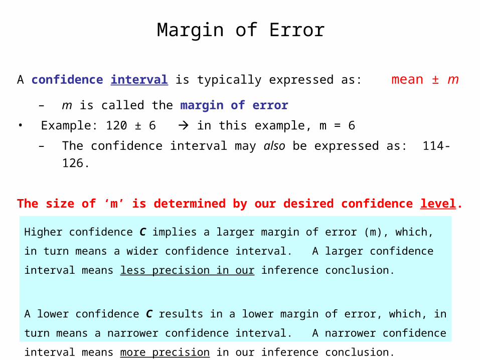
A confidence interval is typically expressed as: mean ± m

– m is called the margin of error

• Example: 120 ± 6 in this example, m = 6

– The confidence interval may also be expressed as: 114-126.

The size of ‘m’ is determined by our desired confidence level.

Margin of Error

Higher confidence C implies a larger margin of error (m), which, in turn means a wider confidence

interval. A larger confidence interval means less precision in our inference conclusion.

A lower confidence C results in a lower margin of error, which, in turn means a narrower

confidence interval. A narrower confidence interval means more precision in our inference

conclusion.

Tradeoff between C and m• The calculated margin of error (m) depends directly on the value we choose

for our confidence level (C). A higher C means a higher m and vice versa. • If you want a higher confidence level (e.g. 99%), then you will have a to accept a

wider margin of error. • Eg: At 95% you may end up with m = 4.2• If you later decided to increase C to 99% you may end up with m = 6.3• We will learn how to determine m shortly.

• Similarly, if you are willing to accept a lower confidence level (e.g. 90%), then you will have the benefit of a smaller margin of error:

• Eg: At C=95% you may end up with m = 3.9• If you later decided to decrease C to 90% you may end up with m = 2.3

Restated: It’s great to have a higher confidence level, but the cost is that we end up with a higher margin of error (i.e. a wider confidence interval).

Calculating the margin of error

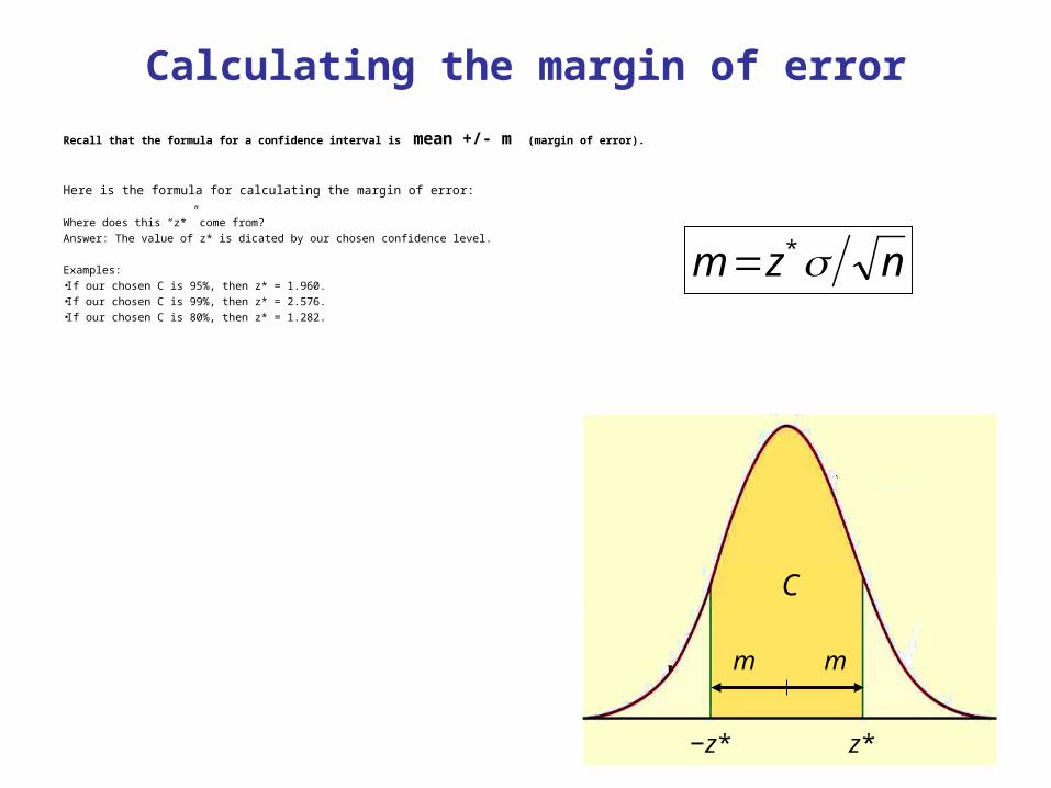
Recall that the formula for a confidence interval is mean +/- m (margin of error).

Here is the formula for calculating the margin of error:

Where does this “z*” come from? Answer: The value of z* is dicated by our chosen confidence level.

Examples: •If our chosen C is 95%, then z* = 1.960.•If our chosen C is 99%, then z* = 2.576.•If our chosen C is 80%, then z* = 1.282.

nzm *

C

z*−z*

m m

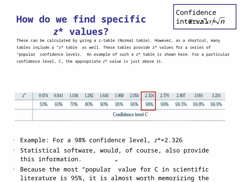
How do we find specific z* values?

These can be calculated by using a z-table (Normal table). However, as a shortcut, many tables include a “z*

table” as well. These tables provide z* values for a series of “popular” confidence levels. An example of such

a z* table is shown here. For a particular confidence level, C, the appropriate z* value is just above it.

• Example: For a 98% confidence level, z*=2.326• Statistical software, would, of course, also provide this information. • Because the most “popular” value for C in scientific literature is 95%, it is almost

worth memorizing the corresponding z* which is 1.96.

nzx *Confidence interval =

Calculating the z*

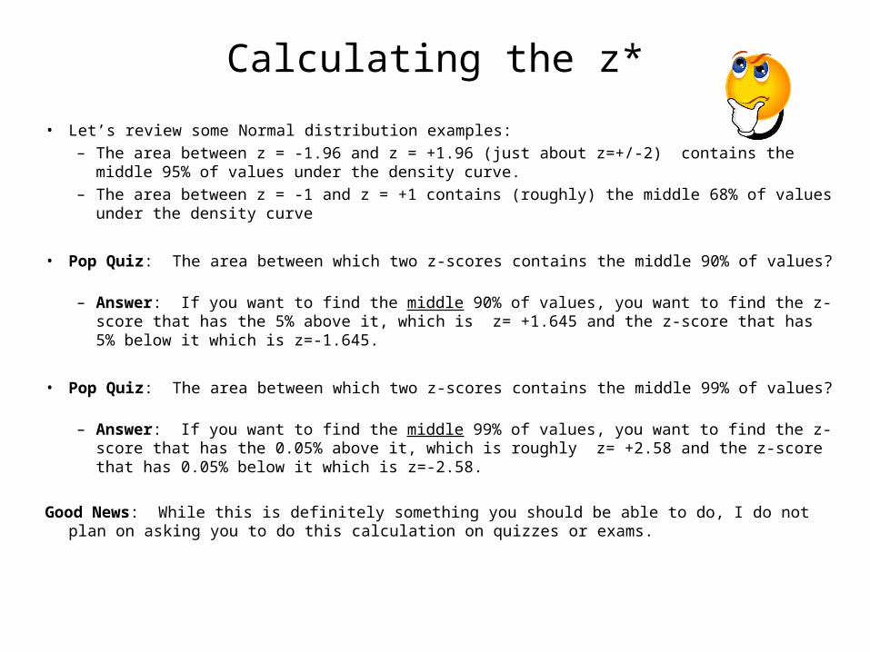
• Let’s review some Normal distribution examples:– The area between z = -1.96 and z = +1.96 (just about z=+/-2) contains the middle 95% of values

under the density curve.– The area between z = -1 and z = +1 contains (roughly) the middle 68% of values under the

density curve

• Pop Quiz: The area between which two z-scores contains the middle 90% of values? – Answer: If you want to find the middle 90% of values, you want to find the z-score that has the

5% above it, which is z= +1.645 and the z-score that has 5% below it which is z=-1.645.

• Pop Quiz: The area between which two z-scores contains the middle 99% of values? – Answer: If you want to find the middle 99% of values, you want to find the z-score that has the

0.05% above it, which is roughly z= +2.58 and the z-score that has 0.05% below it which is z=-2.58.

Good News: While this is definitely something you should be able to do, I do not plan on asking you to do this calculation on quizzes or exams.

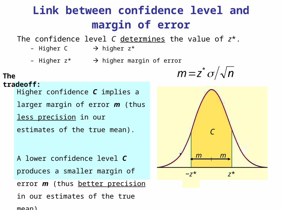
Link between confidence level and margin of error

The confidence level C determines the value of z*. – Higher C higher z*

– Higher z* higher margin of error

nzm *

C

z*−z*

m m

Higher confidence C implies a larger margin

of error m (thus less precision in our

estimates of the true mean).

A lower confidence level C produces a

smaller margin of error m (thus better

precision in our estimates of the true mean).

The tradeoff:

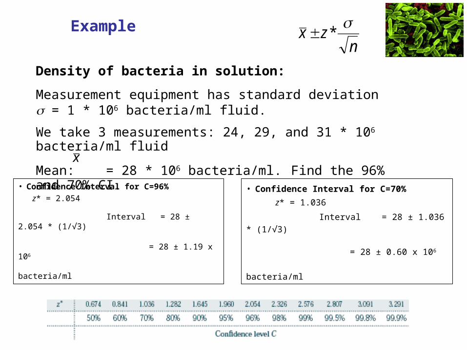
Example

• Confidence Interval for C=96% z* = 2.054

Interval = 28 ± 2.054 * (1/√3)

= 28 ± 1.19 x 106

bacteria/ml

• Confidence Interval for C=70%

z* = 1.036

Interval = 28 ± 1.036 * (1/√3)

= 28 ± 0.60 x 106

bacteria/ml

Density of bacteria in solution:

Measurement equipment has standard deviation = 1 * 106 bacteria/ml fluid.

We take 3 measurements: 24, 29, and 31 * 106 bacteria/ml fluid

Mean: = 28 * 106 bacteria/ml. Find the 96% and 70% CI.

nzx

*

x

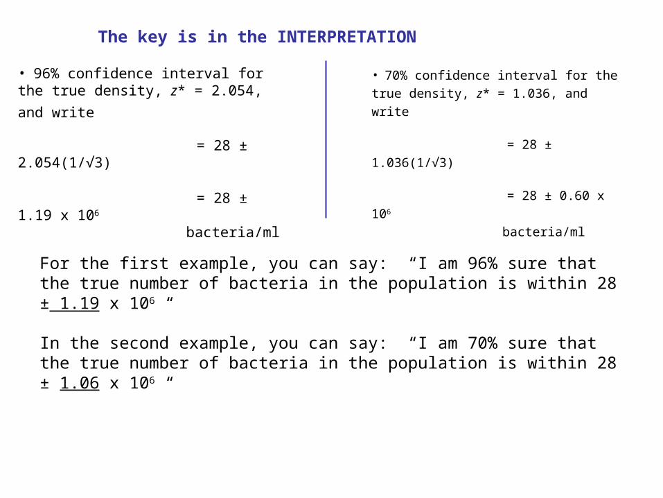
The key is in the INTERPRETATION

• 96% confidence interval for the true

density, z* = 2.054, and write

= 28 ± 2.054(1/√3)

= 28 ± 1.19 x 106

bacteria/ml

• 70% confidence interval for the true density, z* = 1.036, and write

= 28 ± 1.036(1/√3)

= 28 ± 0.60 x 106

bacteria/ml

For the first example, you can say: “I am 96% sure that the true number of bacteria in the population is within 28 ± 1.19 x 106 “

In the second example, you can say: “I am 70% sure that the true number of bacteria in the population is within 28 ± 1.06 x 106 “

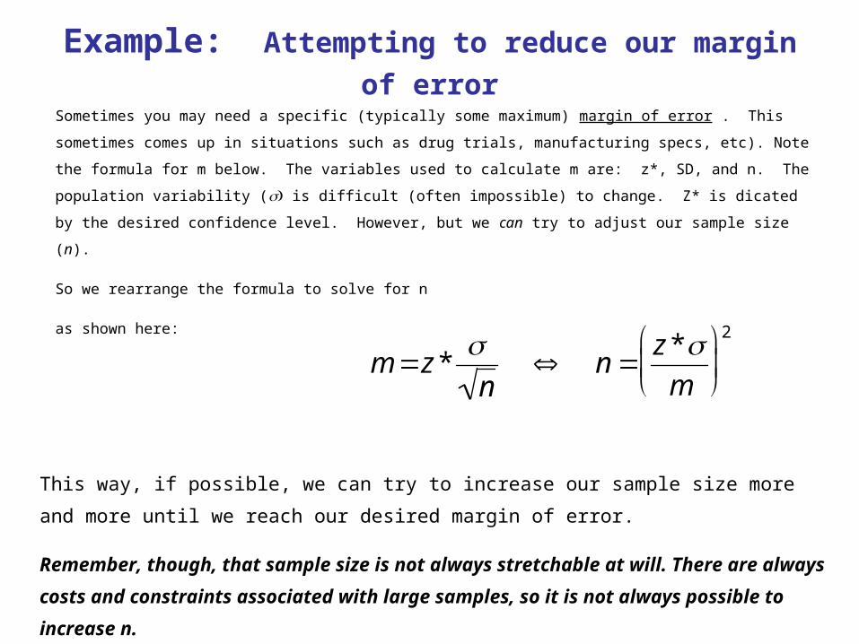
Example: Attempting to reduce our margin of error

Sometimes you may need a specific (typically some maximum) margin of error . This sometimes comes up

in situations such as drug trials, manufacturing specs, etc). Note the formula for m below. The variables

used to calculate m are: z*, SD, and n. The population variability ( is difficult (often impossible) to

change. Z* is dicated by the desired confidence level. However, but we can try to adjust our sample size

(n).

So we rearrange the formula to solve for n

as shown here:

m z *n

n z *

m

2

This way, if possible, we can try to increase our sample size more and more until we reach our desired

margin of error.

Remember, though, that sample size is not always stretchable at will. There are always costs and

constraints associated with large samples, so it is not always possible to increase n.

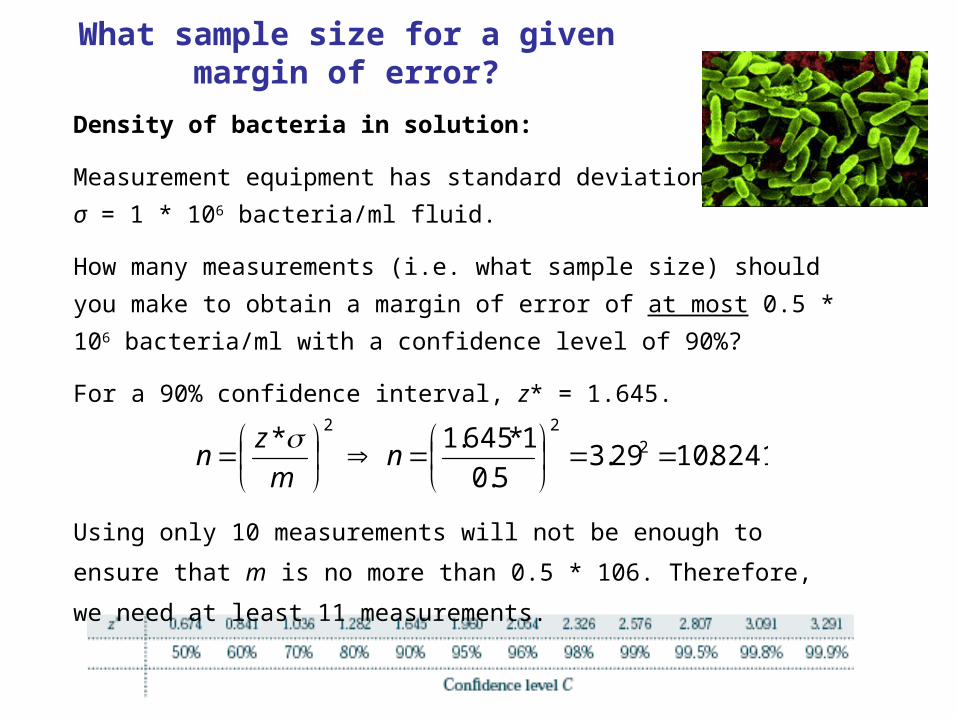
What sample size for a given margin of error?

Density of bacteria in solution:

Measurement equipment has standard deviation

σ = 1 * 106 bacteria/ml fluid.

How many measurements (i.e. what sample size) should you make to

obtain a margin of error of at most 0.5 * 106 bacteria/ml with a

confidence level of 90%?

For a 90% confidence interval, z* = 1.645.

8241.1029.35.0

1*645.1

* 222

n

m

zn

Using only 10 measurements will not be enough to ensure that m is no

more than 0.5 * 106. Therefore, we need at least 11 measurements.