Embed Size (px)
Citation preview

Indoor Navigation System for Handheld Devices
A Major Qualifying Project Report
Submitted to the faculty
of the
Worcester Polytechnic Institute
Worcester, Massachusetts, USA
In partial fulfillment of the requirements of the
Degree of Bachelor of Science
on this day of October 22, 2009
by
__________________________
Manh Hung V. Le
__________________________
Dimitris Saragas
__________________________
Nathan Webb
Advisor __________________________ Advisor __________________________
Professor Alexander Wyglinski Professor Richard Vaz
i
Abstract
This report details the development of an indoor navigation system on a web-enabled smartphone.
Research of previous work in the field preceded the development of a new approach that uses data
from the device’s wireless adapter, accelerometer, and compass to determine user position. A routing
algorithm calculates the optimal path from user position to destination. Testing verified that two meter
accuracy, sufficient for navigation, was achieved. This technique shows promise for future handheld
indoor navigation systems that can be used in malls, museums, hospitals, and college campuses.

ii
Acknowledgements
We would like to sincerely thank the individuals who guided us through our Major Qualifying Project and
who made our experience a memorable one.
We would like to thank our project sponsors, Dr. Sean Mcgrath and Dr. Michael Barry, for providing us
with the necessary information and resources to complete our project.
We would also like to thank our advisors, Professor Richard Vaz and Professor Alexander Wyglinski for
their continuous help and support throughout the project.
iii
Executive Summary
Dashboard mounted GPS receivers and online mapping services have replaced paper maps and atlases
in modern society. Contrasting these advances in automobile navigation, wall mounted maps and signs
continue to be the primary reference for indoor navigation in hospitals, universities, shopping malls, and
other large structures. In this project the development, implementation, and testing of a smartphone-
based indoor navigation system are described.
The HTC Hero was selected as the development platform for this project. Reasons for its selection
include the open-source nature of the Google Android operating system, the large number of sensors
built in to the phone, and the high computational power of the device. Apple iPhone OS was also
considered.
Three primary objectives were identified that summarize the challenges faced in this project. First, the
device must be capable of determining its location in the building. Second, it must be capable of
determining the optimal route to a destination. Third, an intuitive user interface must provide the user
with access to these features.
Numerous candidate positioning techniques and technologies were considered for meeting the first
objective. The decision was made to implement an integrated positioning system making use of multiple
sources of information common to modern smartphones. Signal strength measurements from the
device’s wireless adapter are used to estimate position based on the known locations of wireless access
points. The method used is similar to the calibration-heavy technique of location fingerprinting, but a
pre-generated wireless propagation model is used to alleviate the calibration requirement.
Measurements of acceleration and orientation from the device’s accelerometer and magnetic compass
are used to repeatedly approximate the device’s motion. These sources of information are combined
with information from past sample periods to continually estimate the user location.
To overcome the challenge of determining an optimal path to the user’s destination, the rooms and
hallways of the building were represented as graphical nodes and branches. Many common routing
algorithms were considered for use in determining the best path to the user’s destination in the defined
graph. Dijkstra’s algorithm was chosen for its low computational complexity, its guarantee of
determining the optimal path, and its potential for efficient handling of sparse graphs.
iv
The user interface was developed using the Google Android software development kit and provides the
user with the ability to determine their location, select a destination from a database of people and
places, and follow the route that the phone determines.
Device testing showed that the three primary objectives were accomplished. The integrated positioning
techniques achieved an average deviation between estimated positions and the user’s path of less than
two meters. Matching these position estimates to known paths and locations in the building further
increased the accuracy. Additionally, the location database and routing algorithm accomplished the
objective of optimal routing. A user interface was constructed that allowed access to these functions.
Contributions made through the completion of this project include the use of an integrated propagation
model to simulate wireless propagation and hence negate the need for data collection in a WiFi-
fingerprinting like system. Also, a statistical method was developed for estimating position based on
successive, unreliable, measurements from WiFi positioning and inertial navigation sensors. The
development of these techniques made possible an innovative approach to the challenge of indoor
positioning and navigation that is less difficult to implement and is compatible with existing handheld
devices.
Future directions for research in this area were identified. These include development of an application
that automates conversion of map images into wireless propagation information, incorporation of a
more robust propagation model, and automated accessing of map files hosted on local or remote
servers. Progress in these three areas is deemed necessary for a handheld device application to greatly
improve upon current techniques for indoor navigation.
v
Table of Contents
Abstract ................................................................................................................................................... i
Acknowledgements ................................................................................................................................ ii
Executive Summary ............................................................................................................................... iii
Table of Contents.................................................................................................................................... v
Table of Figures...................................................................................................................................... ix
Table of Tables ....................................................................................................................................... xi
1 Introduction .................................................................................................................................... 1
2 Background Research ...................................................................................................................... 4
2.1 Potential Technologies ................................................................................................................ 4
2.1.1 Satellites............................................................................................................................. 4
2.1.2 Cellular Communication Network ....................................................................................... 5
2.1.3 WiFi .................................................................................................................................... 5
2.1.4 Bluetooth ........................................................................................................................... 6
2.1.5 Infrared .............................................................................................................................. 7
2.1.6 Ultra Wide Band ................................................................................................................. 7
2.1.7 Potential Technology Summary .......................................................................................... 9
2.2 Positioning Techniques ............................................................................................................. 10
2.2.1 Cell of Origin ..................................................................................................................... 10
2.2.2 Angle of Arrival ................................................................................................................. 10
2.2.3 Angle Difference of Arrival ................................................................................................ 11
2.2.4 Time of Arrival .................................................................................................................. 12
2.2.5 Time Difference of Arrival ................................................................................................. 13
2.2.6 Triangulation .................................................................................................................... 14
2.2.7 Location Fingerprinting ..................................................................................................... 14
2.2.8 Positioning Technique Summary ....................................................................................... 15
2.3 Indoor Propagation Models ...................................................................................................... 16
2.3.1 Free Space Model ............................................................................................................. 16
2.3.2 One Slope Model .............................................................................................................. 16
2.3.3 Multi-Wall Model ............................................................................................................. 17

vi
2.3.4 The New Empirical Model ................................................................................................. 18
2.3.5 Modeling Multipath Effects .............................................................................................. 21
2.3.6 Propagation Model Summary ........................................................................................... 22
2.4 Inertial Navigation System ........................................................................................................ 23
2.4.1 Dead Reckoning ................................................................................................................ 24
2.4.2 Map Matching .................................................................................................................. 24
2.5 Mapping Techniques ................................................................................................................. 27
2.5.1 Mapping Information Formats .......................................................................................... 27
2.5.2 Map Creation Techniques ................................................................................................. 28
2.5.3 Graphing Representation .................................................................................................. 28
2.5.4 Routing Algorithm ............................................................................................................ 28
2.6 Mobile Platforms ...................................................................................................................... 37
2.6.1 Apple iPhone OS ............................................................................................................... 37
2.6.2 Google Android ................................................................................................................ 38
2.6.3 Mobile Platform Summary ................................................................................................ 39
2.7 Chapter Summary ..................................................................................................................... 41
3 Project Overview and Design ........................................................................................................ 42
3.1 Goal .......................................................................................................................................... 42
3.2 Objectives ................................................................................................................................. 42
3.3 Design Requirements ................................................................................................................ 43
3.4 Design ....................................................................................................................................... 44
3.5 Positioning Techniques ............................................................................................................. 45
3.6 Mobile Platform ........................................................................................................................ 46
3.7 Summary .................................................................................................................................. 46
4 Positioning .................................................................................................................................... 48
4.1 WiFi Positioning ........................................................................................................................ 48
4.1.1 Propagation Model ........................................................................................................... 48
4.1.2 Accuracy Assessment and Calibration ............................................................................... 49
4.1.3 Location Search Algorithm ................................................................................................ 52
4.2 Inertial Navigation System ........................................................................................................ 55
vii
4.2.1 Calibration ........................................................................................................................ 56
4.2.2 Alignment ......................................................................................................................... 58
4.2.3 Initial Value ...................................................................................................................... 61
4.2.4 Evaluation ........................................................................................................................ 61
4.3 Combining Outputs of WiFi and Inertial Systems ....................................................................... 63
4.3.1 Inertial Navigation Likelihood Function ............................................................................. 63
4.3.2 Combining INS Likelihood Function with Previous Position Estimate ................................. 65
4.3.3 Combining INS-updated Position and WiFi Position Estimate ............................................ 66
4.4 Summary .................................................................................................................................. 66
5 Navigation ..................................................................................................................................... 68
5.1 Graphing ................................................................................................................................... 68
5.2 Routing Algorithm ..................................................................................................................... 69
5.3 Map Matching .......................................................................................................................... 69
5.4 Summary .................................................................................................................................. 71
6 Prototype Implementation ........................................................................................................... 72
6.1 Android Platform Architecture .................................................................................................. 72
6.2 Software System Design ............................................................................................................ 72
6.2.1 Threading and Synchronization ......................................................................................... 73
6.2.2 Source Code Structure ...................................................................................................... 75
6.3 Functional Blocks ...................................................................................................................... 77
6.3.1 Inertial Navigation System ................................................................................................ 77
6.3.2 WiFi Positioning ................................................................................................................ 78
6.3.3 Positioning Fusion ............................................................................................................ 79
6.3.4 Database .......................................................................................................................... 79
6.3.5 Routing ............................................................................................................................. 79
6.4 Graphical User Interface ........................................................................................................... 83
6.4.1 Directory .......................................................................................................................... 85
6.4.2 Routing ............................................................................................................................. 86
6.4.3 Map View ......................................................................................................................... 88
6.5 Summary .................................................................................................................................. 89
viii
7 Testing and Results ....................................................................................................................... 90
7.1 Inertial Navigation System Testing ............................................................................................ 90
7.1.1 Quantitative Inertial Navigation System Testing................................................................ 90
7.1.2 Qualitative Inertial Navigation System Testing .................................................................. 93
7.2 WiFi Positioning System Testing ................................................................................................ 94
7.3 Integrated Positioning System Testing....................................................................................... 95
7.4 Summary .................................................................................................................................. 96
8 Conclusion ..................................................................................................................................... 97
9 Recommendations ........................................................................................................................ 99
9.1 Future Directions ...................................................................................................................... 99
9.2 Opportunity Analysis................................................................................................................. 99
Bibliography........................................................................................................................................ 100
Appendices ......................................................................................................................................... 102
Appendix A: MATLAB Propagation Simulation.................................................................................. 102
Propagation Modeling Function ................................................................................................... 102
Supporting Functions ................................................................................................................... 107
Appendix B: HTC Android Application Source Code .......................................................................... 114
Activity ........................................................................................................................................ 114
Map ............................................................................................................................................. 127
Positioning ................................................................................................................................... 151
View ............................................................................................................................................ 169
Utilities ........................................................................................................................................ 174
Appendix C: Database files............................................................................................................... 182
Nodes.txt ..................................................................................................................................... 182
Edges.txt ...................................................................................................................................... 184
Walls.txt ...................................................................................................................................... 186

ix
Table of Figures
Figure 2-1: Time of Arrival 12
Figure 2-2: Time Difference of Arrival 13
Figure 2-3: Triangulation 14
Figure 2-4: Angle Dependence of Propagation Model: Non-normal Paths Experience Greater Loss 18
Figure 2-5: Partial Obstruction of First Fresnel Zone by Floor and Ceiling 20
Figure 2-6: Simple Diffraction Diagram 22
Figure 2-7: Integration Drift 23
Figure 2-8: Using map matching to estimate the position of the device 25
Figure 2-9: This picture shows possible errors in a map matching algorithm 26
Figure 2-10: Dijkstra’s Diagram at Time 0 after Initialization 29
Figure 2-11: Dijkstra's Diagram Starting from Node 1 30
Figure 2-12: Dijkstra's Diagram when Node 2 is optimized 31
Figure 2-13: Dijkstra's Diagram when Node 4 is optimized 32
Figure 2-14: Dijkstra's Diagram when Node 3 is optimized 32
Figure 2-15: Dijkstra's Diagram when Node 5 is optimized 33
Figure 2-16: Dijkstra's Diagram when the Destination Node is optimized 34
Figure 2-17: The four platform software layers of the iPhone OS (from [20]) 37
Figure 2-18: Google Android Operating System Architecture Framework (from [21]) 39
Figure 2-19: Consumer Popularity of Mobile Platform in July 2009 40
Figure 2-20: Developer Popularity of Mobile Platform in July 2009 41
Figure 3-1: System Design Block Diagram 44
Figure 4-1: Propagation Model Software Flowchart 49
Figure 4-2: Accuracy Testing Points 50
Figure 4-3: Test Results Showing Moderate Correlation between Measured and Predicted Values 50
Figure 4-4: Test Results Showing Strong Correlation between Measured and Predicted Values 51
Figure 4-5: Example Signal Strength Variation 52
Figure 4-6: Received Signal Strength with PDF 54
Figure 4-7: Sample Likelihood Plot (Single WAP) 54
Figure 4-8: Sample Likelihood Plot (Multiple WAPs) 55
Figure 4-9: An inertial navigation system design 55
Figure 4-10: The Earth’s coordination system in three dimensions 59

x
Figure 4-11: Motion Detection from Inertial Navigation System 62
Figure 4-12: Sample INS Likelihood Distribution 65
Figure 4-13: Example Positioning Functionality 67
Figure 5-1: The graph of the 2nd floor of Engineering Research Building 70
Figure 5-2: Map Matching Algorithm example 71
Figure 6-1: Application Software General Functional Blocks 73
Figure 6-2: Application Main Threads and Functions 74
Figure 6-3: Threads & Static Memories Dependencies 75
Figure 6-4: Application Source Code Structure 76
Figure 6-5: Inertial Navigation System Software Flowchart 78
Figure 6-6: Non-optimized Dijkstra Software Flow Chart 80
Figure 6-7: Optimized Dijkstra with Fibonacci Heap Software Flow Chart 82
Figure 6-8: HTC Hero Physical I/O Device for User Interaction 83
Figure 6-9: Application Home Screen 84
Figure 6-10: Application State Map 84
Figure 6-11: Directory View Home Screen and is expanded view 85
Figure 6-12: Direction Pop Up Menu & View Menu Option 86
Figure 6-13: Linking from the Directory screen to Get Direction screen 87
Figure 6-14: Auto-complete feature in Routing GUI 87
Figure 6-15: Map View screen with and without route directions 88
Figure 6-16: Finding the current position of the user and display it on the screen 89
Figure 7-1: INS Test Locations 91
Figure 7-2: Quad-Directional INS Test Results for Standing and Walking Trials 91
Figure 7-3: Direction-Normalized INS Test Results for Standing and Walking Cases 92
Figure 7-4: Histograms of Radial and Angular Data from INS Testing 93
Figure 7-5: Instantaneous WiFi Positioning Plot 94
Figure 7-6: HTC Position Estimates 95
Figure 7-7: Nodes and Links for Map Matching 96
Figure 7-8: Map Matched Position Estimates 96
xi
Table of Tables
Table 2-1: Common RSSI to RSS conversions [10] 6
Table 2-2: Pros and cons of the possible reference signals 9
Table 2-3: Pros and cons of each positioning technique 15
Table 2-4: One Slope Model Exponent Values [7] 17
Table 2-5: Breakpoint Distances for Common Frequencies 20
Table 2-6: Diffraction Coefficients [16] 21
Table 2-7: Pros and cons of each propagation model 22
Table 2-8: Pros and cons of each possible routing algorithm 36
Table 2-9: Pros and cons of each mobile platform 41
Table 3-1: The design requirements include four subsystems and their descriptions 43
Table 3-2: The HTC Hero specification sheet [23] 47
Table 4-1: The accelerometer output in the three positions 57
Table 4-2: A sample of the compass’ output 58
1
1 Introduction
Technological advances within the past decade have caused a surge in the proliferation of personal
locating technologies. Early consumer grade locating systems manifested as Global Position System
(GPS) receivers fit for mounting on automobiles, aircraft, and watercraft. As computing and
communication technologies have advanced, companies including Garmin Ltd., TomTom International,
and Magellan Navigation Inc. have offered systems with increased usability and functionality. Current
systems on the dashboard mounted, handheld, and wristwatch scales provide users the ability to
determine their current location and find their way to their destination. Today’s advanced systems use
measurements of signals from GPS, cellular communication towers, and wireless internet (WiFi) access
points to locate the user.
Internet enabled mobile devices are becoming ubiquitous in the personal and business marketplaces.
Integration of locating technologies into these smartphones has made the use of handheld devices that
are dedicated to positioning obsolete. The availability of powerful communication and computing
systems on the handheld scale has created many opportunities for readdressing problems that have
historically been solved in other ways.
One such problem is indoor navigation. The signals used by outdoor locating technologies are often
inadequate in this setting. Systems that rely on the use of cellular communication signals or
identification of nearby WiFi access points do not provide sufficient accuracy to discriminate between
the individual rooms of a building. GPS based systems can achieve sufficient accuracy, but are unreliable
indoors due to signal interference caused by walls, floors, furniture, and other objects. Due to these
limitations, navigation inside unfamiliar buildings is still accomplished by studying large maps posted in
building lobbies and common areas. If created, a system capable of locating a person and directing
them to their destination would be more convenient and would provide functionality that a static wall
map cannot.
Research into indoor positioning systems has identified some possible technologies, but none of these
has been developed and distributed to consumers. One possibility is to install transmitters in the
building to reproduce GPS signals. Implementation of this approach, called Pseudolite GPS, can yield
high accuracy [1]. An alternate approach is to install electromagnetic reference beacons within the
building that can be used to triangulate a devices position. This approach has been tested using a
2
variety of reference signals; Ultra-Wideband [2], Bluetooth [3], and Radio Frequency [4] are among the
most common. WiFi access point fingerprinting is a third approach. It is desirable because it does not
necessitate the installation of additional transmitters; it makes use of existing WiFi access points [5].
Though there is no hardware installation requirement, implementing a WiFi fingerprinting based system
requires the user to characterize their indoor environment by taking myriad measurements throughout
the structure. It was determined that an indoor location system based on any of these techniques was
feasible, but they present implementation and compatibility challenges that make them unfit for use in
an ubiquitous handheld device based system.
In this project, an indoor navigation system that provides positioning and navigation capabilities is
proposed and tested. The hardware installation requirement is alleviated through the use of existing
WiFi access points and through the integration of the final software application with a popular
smartphone. While previous systems that make use of WiFi access points require a lengthy period of
data collection and calibration, this system does not. Data on the positions of walls and WiFi access
points in the building is used to simulate WiFi fingerprint data without a time-consuming measurement
requirement.
The WiFi positioning capability is augmented through the use of two other sensors common to
smartphones: an inertial sensor typically used to characterize phone motion, and a magnetic sensor that
acts as the phones compass in traditional navigation applications. Taken together, these sensors can be
used to form a rudimentary inertial navigation system (INS) that estimates the nature and direction of a
user’s motion. Tracking a moving user’s location in the building is better accomplished by combining
this information with the output of the WiFi positioning system.
In addition to the positioning subsystem, a database and a navigation system are implemented to
increase system usability. The database allows the user to search a directory of people and places
within the building. The navigation subsystem informs the user of the optimal route to their
destination. These system components form a software application that is accessible through an
intuitive user interface.
Through completion of this project, contributions have been made to the indoor positioning knowledge
base. An integrated propagation model was used to simulate wireless propagation and negate the need
for data collection in a WiFi-fingerprinting like system. Also, a statistical method was developed for
estimating position based on successive, unreliable, measurements from WiFi positioning and inertial
3
navigation sensors. The development of these techniques made possible an innovative approach to the
challenge of indoor navigation.
The remainder of this report is structured to first provide the reader with background information
(Chapter 2) in the relevant areas of wireless positioning technologies, common positioning techniques,
WiFi propagation, mapping, INS, navigation, and smartphone platforms. Chapter 3 contains an overview
of the project including goals, and objectives. It also details the design choices and system architecture,
as well as the design requirements that led to them. Chapters 4, 5, and 6 are detailed descriptions of
the positioning, navigation, and software application, respectively. Chapter 7 describes system testing.
Chapter 8 contains conclusions drawn about the process used and result reached, with regards to the
design choices made, as well as the overall system. Chapter 9 contains recommendations for future
work, as well as an analysis of opportunities to apply knowledge gained through designing this system.
Following the body of the report, appendices contain relevant information that was either unnecessary
or too large to include in the main text.
4
2 Background Research
The proliferation of mobile devices and the growing demand for location aware systems that filter
information based on current device location have led to an increase in research and product
development in this field [4]. However, most efforts have focused on the usability aspect of the
problem and have failed to develop innovative techniques that address the essential challenge of this
problem: the positioning technique itself. This section describes various techniques for positioning and
navigation that have been researched before and are applicable to this project.
2.1 Potential Technologies
The follow section describes reference signals considered for use in this system.
2.1.1 Satellites
Satellite navigation systems provide geo-spatial positioning with global coverage. Currently there are
several global navigation satellite systems dedicated to civil positioning including the US NAVSTAR
Global Positioning System (GPS), the Russian GLONASS, and the European Union’s Galileo [6]. The
advantage of satellite systems is that receivers can determine latitude, longitude, and altitude to a high
degree of accuracy. However, line of sight (LOS) is required for the functioning of these systems. This
leads to an inability to use these systems for an indoor environment where the LOS is blocked by walls
and roofs.
GPS is a semi-accurate global positioning and navigating system for outdoor applications [7]. The GPS
system consists of 24 satellites equally spaced in six orbital planes 20,200 km above the Earth [8]. The
accuracy of GPS devices is consistently improving but is still in the range of 5-6 meters in open space. A
GPS device cannot be used for an indoor environment because the LOS is blocked.
Methods have been developed to overcome the LOS requirement of GPS by setting up pseudolite
systems that imitate GPS satellites by sending GPS-like correction signals to receiver within the building.
A system has been developed by the Seoul National University GPS Lab, which achieves sub-centimeter
accuracy for indoor GPS navigation system [1]. This system has a convergence time of under 0.1
seconds, which helps to increase the responsiveness for a mobile user. This system uses pseudolites and
a reference station to assist a GPS mobile vehicle in an indoor environment. The pseudolites have a
fixed position and use an inverse carrier phase differential GPS to calculate the mobile user’s position.
The reference station is also fixed and transmits carrier phase correction to the mobile user. The system

5
faces several challenges including serious multipath propagation errors and strict pseudolite
synchronization requirements. The multipath propagation is addressed through the use of a pulse
scheme. Using a center pseudolite solves the synchronization problem. The prototype has achieved
0.14 cm static error and 0.79 cm dynamic error. However, this system is very financially costly to
implement, due to the requirement for a large number of pseudolites.
Assisted GPS (A-GPS) is primarily used in cellular phones [7]. The A-GPS method uses assistance from a
third party service provider, such as a cell phone network, to assist the mobile device by instructing it to
search for particular satellite. Also, data from the device itself is used to perform positioning calculations
that might not otherwise be possible due to limited computational power. A-GPS is useful when some
satellite signals are weak or unavailable. The cell tower provides information that assists the GPS
receiver. When using A-GPS, accuracy is typically around 10-20 meters but suffers similar indoor
limitations to standalone GPS [7].
2.1.2 Cellular Communication Network
A Cellular Communication Network is a system that allows mobile phones to communicate with each
other. This system uses large cell towers to wirelessly connect mobile devices. The range of cellular
communication networks depends on the density of large buildings, trees and other possible
obstructions. Maximum range for a cell tower is 35 kilometers in an open rural area [9]. This method is
a basic technique using Cell-ID, also called Cell of Origin, to provide location services for cell phone users
[8]. This method is based on the capability of the network to estimate the position of a cell phone by
identifying the cell tower that the device is using at a specific time. The advantage of this technique is
its ubiquitous distribution, easy implementation and the fact that all mobile cell phones support it. The
accuracy of this technique is very low due to the fact that cell towers can support ranges of 35
kilometers or more. In urban environments cell towers are distributed more densely.
2.1.3 WiFi
Wireless Fidelity (WiFi) is the common nickname for the IEEE 802.11 standard. Wireless connectivity is
more prevalent than ever in our everyday lives. Each wireless router broadcasts a signal that is received
by devices in the area. Wireless devices have the capability to measure the strength of this signal. This
strength is converted to a number, known as received signal strength indicator (RSSI). A user’s device
can detect the RSSI and MAC address of multiple routers at one time.
6
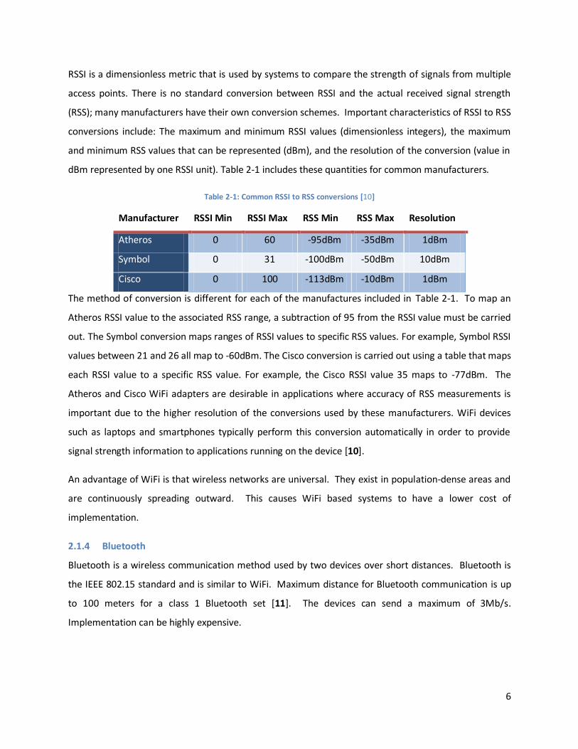
RSSI is a dimensionless metric that is used by systems to compare the strength of signals from multiple
access points. There is no standard conversion between RSSI and the actual received signal strength
(RSS); many manufacturers have their own conversion schemes. Important characteristics of RSSI to RSS
conversions include: The maximum and minimum RSSI values (dimensionless integers), the maximum
and minimum RSS values that can be represented (dBm), and the resolution of the conversion (value in
dBm represented by one RSSI unit). Table 2-1 includes these quantities for common manufacturers.
Table 2-1: Common RSSI to RSS conversions [10]
Manufacturer RSSI Min RSSI Max RSS Min RSS Max Resolution
Atheros 0 60 -95dBm -35dBm 1dBm
Symbol 0 31 -100dBm -50dBm 10dBm
Cisco 0 100 -113dBm -10dBm 1dBm
The method of conversion is different for each of the manufactures included in Table 2-1. To map an
Atheros RSSI value to the associated RSS range, a subtraction of 95 from the RSSI value must be carried
out. The Symbol conversion maps ranges of RSSI values to specific RSS values. For example, Symbol RSSI
values between 21 and 26 all map to -60dBm. The Cisco conversion is carried out using a table that maps
each RSSI value to a specific RSS value. For example, the Cisco RSSI value 35 maps to -77dBm. The
Atheros and Cisco WiFi adapters are desirable in applications where accuracy of RSS measurements is
important due to the higher resolution of the conversions used by these manufacturers. WiFi devices
such as laptops and smartphones typically perform this conversion automatically in order to provide
signal strength information to applications running on the device [10].
An advantage of WiFi is that wireless networks are universal. They exist in population-dense areas and
are continuously spreading outward. This causes WiFi based systems to have a lower cost of
implementation.
2.1.4 Bluetooth
Bluetooth is a wireless communication method used by two devices over short distances. Bluetooth is
the IEEE 802.15 standard and is similar to WiFi. Maximum distance for Bluetooth communication is up
to 100 meters for a class 1 Bluetooth set [11]. The devices can send a maximum of 3Mb/s.
Implementation can be highly expensive.
7
2.1.5 Infrared
Infrared (IR) wireless networking was a pioneer technology in the field of indoor positioning [4].
However, this system has faced several fundamental problems. The primary challenge is the limited
range of an IR network. Also, Infrared does not have any method for providing data networking
services.
An early implementation of an IR technique is the Active Badge System. This is a remote positioning
system in which the location of a person is determined from the unique IR signal emitted every ten
seconds by a badge they are wearing. The signals are captured by sensors placed at various locations
inside a building and relay information to a central location manager system. The accuracy achieved
from this system is fairly high in indoor environments. However, the system suffers from several
limitations such as the sensor installation cost due to the limited range of IR, maintenance cost, and the
receiver’s sensitivity to sunlight, which often occurs in rooms with windows.
2.1.6 Ultra Wide Band
Ultra-wideband (UWB) signals used for positioning are receiving increased attention recently due to
their capability of providing centimeter accurate positioning information [2]. UWB advantages include
low power density and wide bandwidth, which increases the reliability. The use of a wide range of
frequency components increases the probability that a signal will go around an obstacle, offering higher
resolution. Also, the system is subject to less interference from other radio frequencies that are in use in
the area. The nature of the UWB signal allows the time delay approach to provide higher accuracy than
signal strength or directional approaches because the accuracy of time delay positioning is inversly
proportional to the effective bandwidth of the signals. This is shown in the formulas given below.
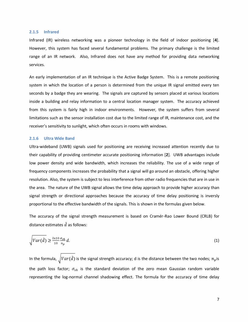
The accuracy of the signal strength measurement is based on Cramér-Rao Lower Bound (CRLB) for
distance estimates as follows:
. (1)
In the formula, is the signal strength accuracy; d is the distance between the two nodes; is
the path loss factor; is the standard deviation of the zero mean Gaussian random variable
representing the log-normal channel shadowing effect. The formula for the accuracy of time delay
8
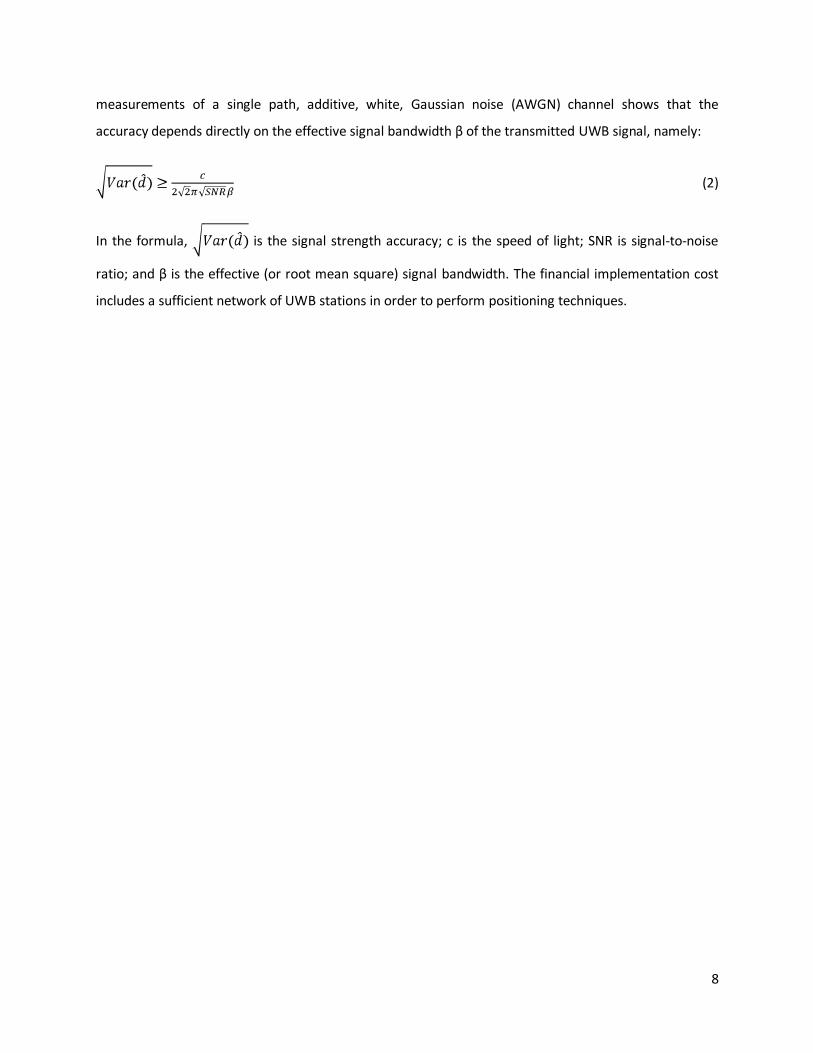
measurements of a single path, additive, white, Gaussian noise (AWGN) channel shows that the
accuracy depends directly on the effective signal bandwidth β of the transmitted UWB signal, namely:
(2)
In the formula, is the signal strength accuracy; c is the speed of light; SNR is signal-to-noise
ratio; and β is the effective (or root mean square) signal bandwidth. The financial implementation cost
includes a sufficient network of UWB stations in order to perform positioning techniques.
9
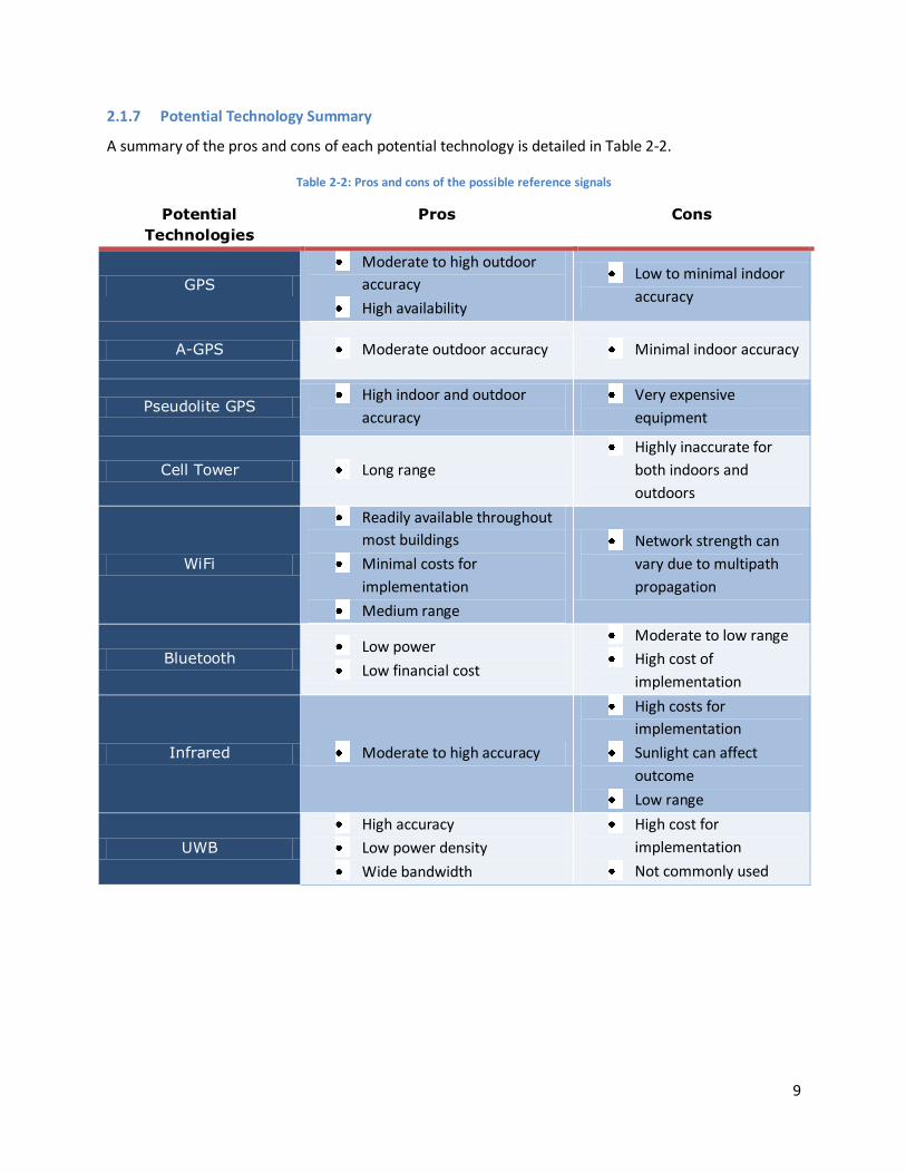
2.1.7 Potential Technology Summary
A summary of the pros and cons of each potential technology is detailed in Table 2-2.
Table 2-2: Pros and cons of the possible reference signals
Potential
Technologies
Pros Cons
GPS
Moderate to high outdoor
accuracy
High availability
Low to minimal indoor
accuracy
A-GPS Moderate outdoor accuracy Minimal indoor accuracy
Pseudolite GPS High indoor and outdoor
accuracy
Very expensive
equipment
Cell Tower Long range
Highly inaccurate for
both indoors and
outdoors
WiFi
Readily available throughout
most buildings
Minimal costs for
implementation
Medium range
Network strength can
vary due to multipath
propagation
Bluetooth Low power
Low financial cost
Moderate to low range
High cost of
implementation
Infrared Moderate to high accuracy
High costs for
implementation
Sunlight can affect
outcome
Low range
UWB
High accuracy
Low power density
Wide bandwidth
High cost for
implementation
Not commonly used
10
2.2 Positioning Techniques
In order to navigate within a building, one must first determine one’s current location. In this section,
multiple positioning techniques are described. Two factors of particular importance in the consideration
of positioning techniques are accuracy and convergence time. These factors should be for the case in
which the device determining the position is stationary and for the case in which the device is moving.
There are two different methods for implementing a positioning system: self and remote positioning [8].
In self-positioning, the physical location is self-determined by the user’s device using transmitted signals
from terrestrial or satellite beacons. The location is known by the user and can be used by applications
and services operating on the user’s mobile device. In remote positioning, the location is determined at
the server side using signals emitted from the user device. The location is then either used by the server
in a tracking software system, or transmitted back to the device through a data transfer method.
The performance of a positioning and navigation system is typically rated on four different aspects that
civil aviation authorities have defined for their systems: accuracy, integrity, availability and continuity
[12]. These parameters focus on addressing the service quality for the mobile user including navigation
service and coverage area. The accuracy of a system is a measure of the probability that the user
experiences an error at a location and at a given time. The integrity of a system is a measure of the
probability that the accuracy error is within a specified limit. The availability of a system is a measure of
its capability to meet accuracy and integrity requirements simultaneously. The continuity of a system is
a measure of the minimum time interval for which the service is available to the user. These concepts
will be used later to evaluate the quality of service of the system created in this project. The errors and
capabilities of this system will be analyzed and stated explicitly.
2.2.1 Cell of Origin
Cell-of-origin systems use information from cellular information towers to inform a user of their
approximate location [7]. COO determines the Cell tower to which the user is closest. Cell sizes can
range from hundreds of meters to dozens of kilometers [9]. While directionality and timing
measurements can be used to improve accuracy, indoor accuracy remains in the hundreds of meters at
best.
2.2.2 Angle of Arrival
Angle of arrival (AOA) is a remote positioning method that makes use of multiple base stations to
approximate a user’s location [7]. In an AOA remote positioning system, two base stations of known
11
position and orientation must determine the angle at which the signal from the user arrived. The angle
is determined by steering a directional antenna beam until the maximum signal strength acquired or its
coherent phase is detected. The position is determined by the intersection of the locus of each of base
station AOA measurement, which is a straight line. If the user and the base stations are not coplanar
then three-dimensional directional antennas are required. The use of more base stations than required
can greatly improve accuracy. The overall accuracy of the system depends on signal propagation, the
accuracy of the directional antennas used and the distance from the antennas to the device.
2.2.3 Angle Difference of Arrival
Angle difference of arrival (ADOA) is a self-positioning method that makes use of multiple base stations
to approximate a user’s location [13]. In an ADOA positioning system a device equipped with a
directional antenna must determine the relative angle at which signals from three base stations of
known location arrived. The requirement for an additional base station develops due to the unknown
orientation of the user. If the user and the base stations are not coplanar then three-dimensional
directional antennas are required. Otherwise, two-dimensional arrays are sufficient. The use of more
base stations than required can greatly improve accuracy. The overall accuracy of the system depends
on signal propagation and the accuracy of the directional antennas used.
12
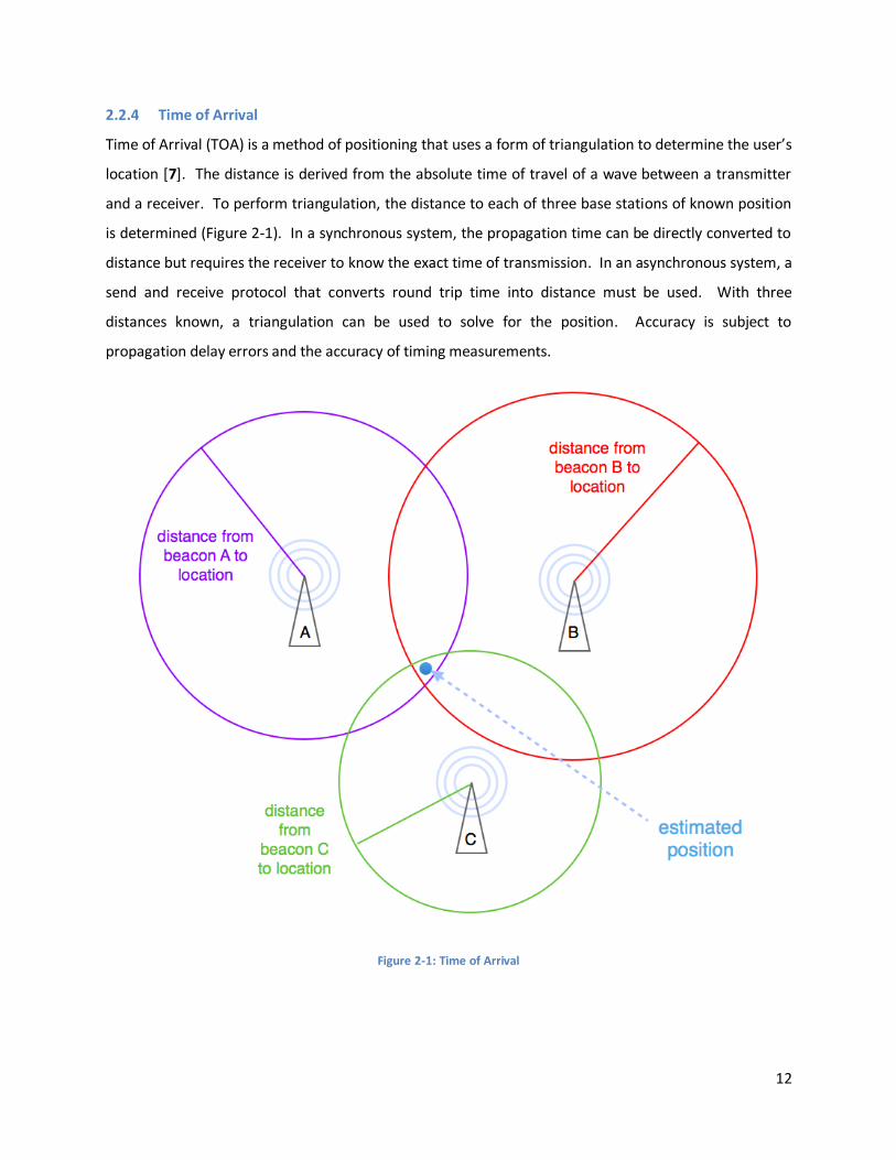
2.2.4 Time of Arrival
Time of Arrival (TOA) is a method of positioning that uses a form of triangulation to determine the user’s
location [7]. The distance is derived from the absolute time of travel of a wave between a transmitter
and a receiver. To perform triangulation, the distance to each of three base stations of known position
is determined (Figure 2-1). In a synchronous system, the propagation time can be directly converted to
distance but requires the receiver to know the exact time of transmission. In an asynchronous system, a
send and receive protocol that converts round trip time into distance must be used. With three
distances known, a triangulation can be used to solve for the position. Accuracy is subject to
propagation delay errors and the accuracy of timing measurements.
Figure 2-1: Time of Arrival
13
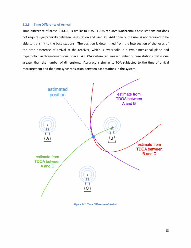
2.2.5 Time Difference of Arrival
Time difference of arrival (TDOA) is similar to TOA. TDOA requires synchronous base stations but does
not require synchronicity between base station and user [7]. Additionally, the user is not required to be
able to transmit to the base stations. The position is determined from the intersection of the locus of
the time difference of arrival at the receiver, which is hyperbolic in a two-dimensional plane and
hyperboloid in three-dimensional space. A TDOA system requires a number of base stations that is one
greater than the number of dimensions. Accuracy is similar to TOA subjected to the time of arrival
measurement and the time synchronization between base stations in the system.
Figure 2-2: Time Difference of Arrival
14
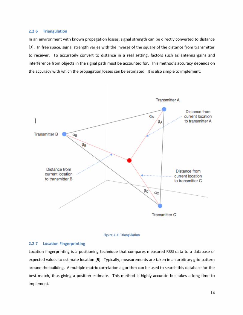
2.2.6 Triangulation
In an environment with known propagation losses, signal strength can be directly converted to distance
[7]. In free space, signal strength varies with the inverse of the square of the distance from transmitter
to receiver. To accurately convert to distance in a real setting, factors such as antenna gains and
interference from objects in the signal path must be accounted for. This method’s accuracy depends on
the accuracy with which the propagation losses can be estimated. It is also simple to implement.
Figure 2-3: Triangulation
2.2.7 Location Fingerprinting
Location fingerprinting is a positioning technique that compares measured RSSI data to a database of
expected values to estimate location [5]. Typically, measurements are taken in an arbitrary grid pattern
around the building. A multiple matrix correlation algorithm can be used to search this database for the
best match, thus giving a position estimate. This method is highly accurate but takes a long time to
implement.
15
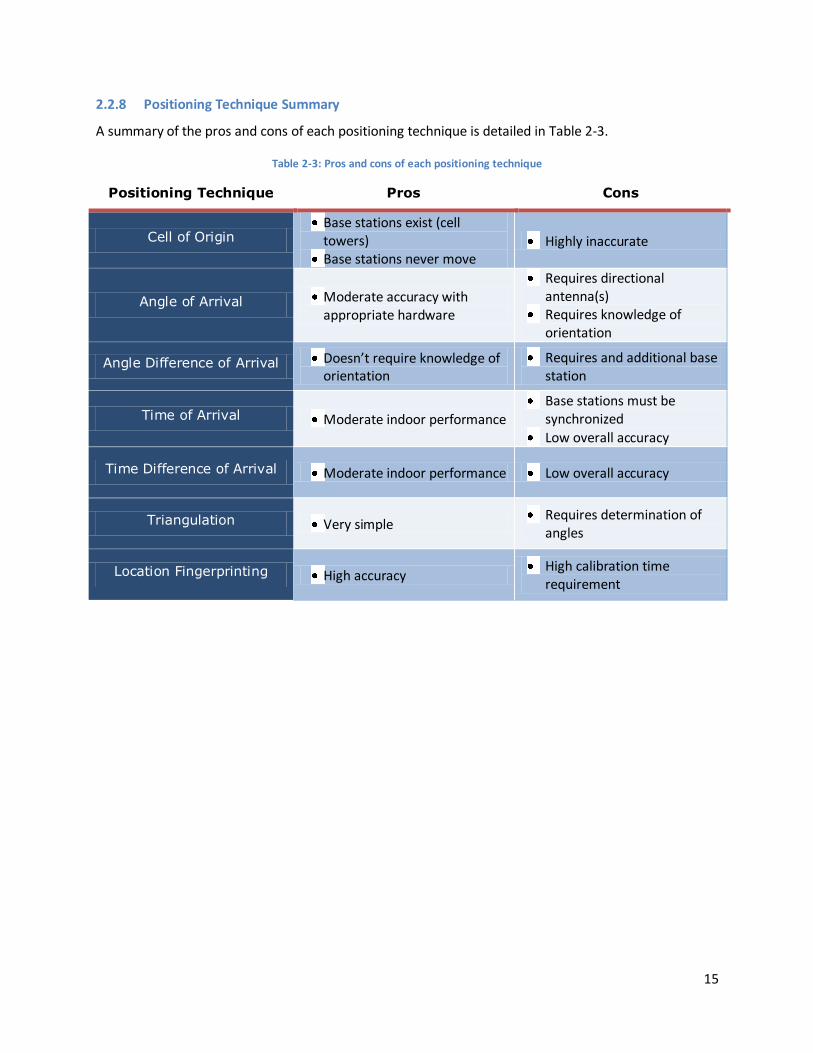
2.2.8 Positioning Technique Summary
A summary of the pros and cons of each positioning technique is detailed in Table 2-3.
Table 2-3: Pros and cons of each positioning technique
Positioning Technique Pros Cons
Cell of Origin Base stations exist (cell towers)
Base stations never move Highly inaccurate
Angle of Arrival Moderate accuracy with appropriate hardware
Requires directional antenna(s)
Requires knowledge of orientation
Angle Difference of Arrival Doesn’t require knowledge of orientation
Requires and additional base station
Time of Arrival Moderate indoor performance
Base stations must be synchronized
Low overall accuracy
Time Difference of Arrival Moderate indoor performance Low overall accuracy
Triangulation Very simple Requires determination of
angles
Location Fingerprinting High accuracy High calibration time
requirement
16
2.3 Indoor Propagation Models
To accurately determine an indoor location using wireless signals as references, an accurate model of
signal propagation is necessary. Received signal strengths are affected by walls, people, furniture, and
other objects, as well as multipath phenomenon. To accurately simulate these effects, multiple models
are considered.
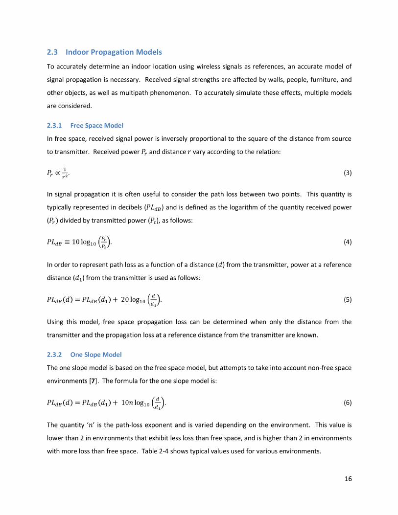
2.3.1 Free Space Model
In free space, received signal power is inversely proportional to the square of the distance from source
to transmitter. Received power and distance vary according to the relation:
. (3)
In signal propagation it is often useful to consider the path loss between two points. This quantity is
typically represented in decibels ( ) and is defined as the logarithm of the quantity received power
( divided by transmitted power ( ), as follows:
. (4)
In order to represent path loss as a function of a distance ( ) from the transmitter, power at a reference
distance ( ) from the transmitter is used as follows:
. (5)
Using this model, free space propagation loss can be determined when only the distance from the
transmitter and the propagation loss at a reference distance from the transmitter are known.
2.3.2 One Slope Model
The one slope model is based on the free space model, but attempts to take into account non-free space
environments [7]. The formula for the one slope model is:
. (6)
The quantity ‘ ’ is the path-loss exponent and is varied depending on the environment. This value is
lower than 2 in environments that exhibit less loss than free space, and is higher than 2 in environments
with more loss than free space. Table 2-4 shows typical values used for various environments.
17
Table 2-4: One Slope Model Exponent Values [7]
Environment Path-loss exponent
Free Space 2.0
Urban Area Cellular 2.7 – 4.0
Shadowed Urban Cellular 3.0 – 5.0
In-Building Line of Sight 1.6 – 1.8
In-Factory Line of Sight 1.6 – 2.0
In-Building One-Floor non-Line of Sight 2.0 – 4.0
Obstructed In-Building 4.0 – 6.0
Obstructed In-Factory 2.0 – 3.0
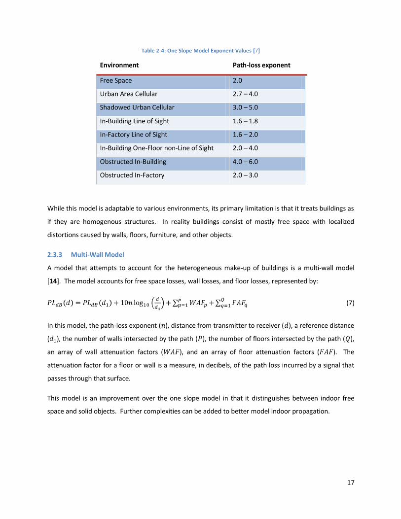
While this model is adaptable to various environments, its primary limitation is that it treats buildings as
if they are homogenous structures. In reality buildings consist of mostly free space with localized
distortions caused by walls, floors, furniture, and other objects.
2.3.3 Multi-Wall Model
A model that attempts to account for the heterogeneous make-up of buildings is a multi-wall model
[14]. The model accounts for free space losses, wall losses, and floor losses, represented by:
(7)
In this model, the path-loss exponent ( ), distance from transmitter to receiver ( ), a reference distance
( ), the number of walls intersected by the path ( ), the number of floors intersected by the path ( ),
an array of wall attenuation factors ( ), and an array of floor attenuation factors ( ). The
attenuation factor for a floor or wall is a measure, in decibels, of the path loss incurred by a signal that
passes through that surface.
This model is an improvement over the one slope model in that it distinguishes between indoor free
space and solid objects. Further complexities can be added to better model indoor propagation.
18
2.3.4 The New Empirical Model
Cheung et al. have proposed a model that takes into account angles of incidence on walls and floors, as
well as a commonly observed break point phenomenon [14]. The reasons for these additions are
further explained in sections 2.3.4.1 and 2.3.4.2. In the model:
, (8)
there are two path-loss exponents ( ) and ( ). The first exponent models losses at distances (d)
between the reference distance (d1) and the break point distance ( ). The second exponent models
losses at distances (d) greater than the breakpoint distance. As in the multi-wall model, other included
terms are: the number of walls intersected by the path ( ), the number of floors intersected by the path
( ), an array of wall attenuation factors ( ), and an array of floor attenuation factors ( ). The
angles and are angles of incidence between the propagation path and the surfaces it passes
through.
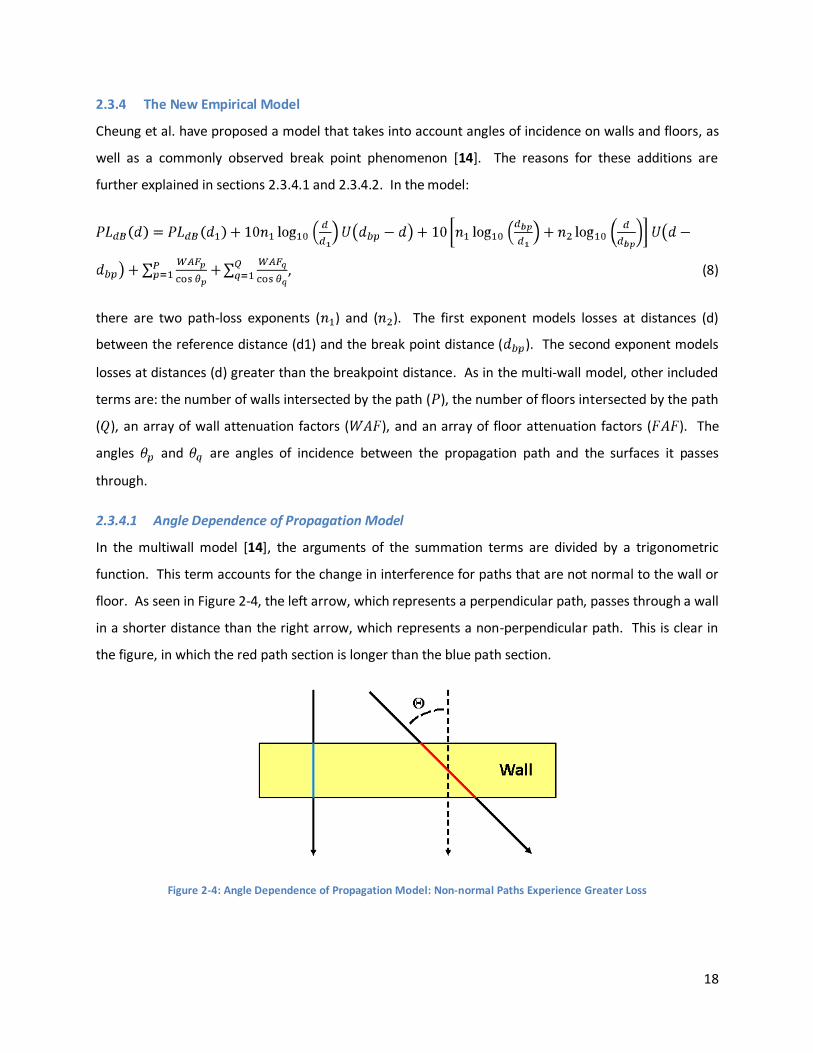
2.3.4.1 Angle Dependence of Propagation Model
In the multiwall model [14], the arguments of the summation terms are divided by a trigonometric
function. This term accounts for the change in interference for paths that are not normal to the wall or
floor. As seen in Figure 2-4, the left arrow, which represents a perpendicular path, passes through a wall
in a shorter distance than the right arrow, which represents a non-perpendicular path. This is clear in
the figure, in which the red path section is longer than the blue path section.
Figure 2-4: Angle Dependence of Propagation Model: Non-normal Paths Experience Greater Loss
19
2.3.4.2 Break Point Phenomenon
The break point concept incorporated into the new empirical model hinges on the concept of Fresnel
zones [14]. To develop the concept of Fresnel zones, first consider the straight line path TR between a
transmitter T and a receiver R. Next consider a plane P that intersects and is perpendicular to TR. Next,
in plane P, construct a circle C with its center at the intersection of P and TR. Any path TCR that passes
from point T to a point on C, and then from a point on C to point R is longer than the straight line path
TR. The path-length difference between TR and TCR increases from zero to infinity as the radius of C is
increased. There then exists for any signal frequency a family of circles with the property that the path
TCR is an odd multiple of radians out of phase with the straight-line path (for example: , , , and so
forth). It is clear that the radius of varies according to the location of plane P along path TR. Each circle
will have its greatest radius at the midpoint of TR. It can be shown that the set of each circle C, one
located at each of the infinite set of locations of P between T and R, defines an ellipsoid of revolution E
with foci at T and R. It is clear that as there is a set of concentric circles in each plane, there is also a set
of concentric ellipsoids. The region within the smallest ellipsoid and the regions that lay between each
consecutive pair of ellipsoids are called Fresnel zones and are denoted F1, F2, F3, and so forth.
Contributions from signals passing through successive Fresnel zones are in phase opposition due to the
difference in path lengths. Signals passing through odd Fresnel zones are between and radians out
of phase with the path TR and so contribute constructive interference. Signals passing through even
Fresnel zones are between and radians out of phase with the path TR and so contribute destructive
interference. Signal density is greatest near the straight line path, so interference with lower numbered
Fresnel zones causes greater effects. Interference with the zone F1 can lead to path losses far greater
than those experienced in free space. For this reason, it is desirable to keep the first Fresnel zone free
of obstruction in radio communication systems [15].
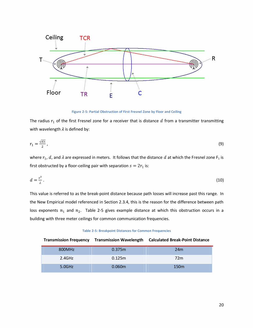
In the case of indoor propagation, line-of-sight paths between transmitter and receiver often do not
exist. While it is impractical to calculate the impact of all obstacles on the infinite number of Fresnel
zones, a common simplification in indoor settings is to determine the distance between transmitter and
receiver at which the floor and ceiling begin to obstruct the first Fresnel zone. An example of this
situation is illustrated in Figure 2-5.
20
Figure 2-5: Partial Obstruction of First Fresnel Zone by Floor and Ceiling
The radius of the first Fresnel zone for a receiver that is distance from a transmitter transmitting
with wavelength is defined by:
, (9)
where , , and are expressed in meters. It follows that the distance at which the Fresnel zone F1 is
first obstructed by a floor-ceiling pair with separation is:
. (10)
This value is referred to as the break-point distance because path losses will increase past this range. In
the New Empirical model referenced in Section 2.3.4, this is the reason for the difference between path
loss exponents and . Table 2-5 gives example distance at which this obstruction occurs in a
building with three meter ceilings for common communication frequencies.
Table 2-5: Breakpoint Distances for Common Frequencies
Transmission Frequency Transmission Wavelength Calculated Break-Point Distance
800MHz 0.375m 24m
2.4GHz 0.125m 72m
5.0GHz 0.060m 150m

21
As can be seen in Table 2-5, the breakpoint is typically distant at high frequencies when the floor-ceiling
separation limits the Fresnel zone’s major diameter. Other limitations, most notably widths of hallways,
can cause the observed breakpoint distance to be smaller than the calculated distance.
2.3.5 Modeling Multipath Effects
In non free-space environments, paths other than the direct path from transmitter to receiver must be
considered. Though the breakpoint phenomenon discussed in Section Paths that include reflection and
diffraction can often increase or decreases the signal strength at a point.
In a typical indoor setting there exist many corners and edges that can contribute to diffraction. To
model this phenomenon in simulations, the diffracted path is usually divided into sections. As in:
, (11)
separate terms are used for propagation from source to edge, diffraction at the edge, and propagation
from edge to destination. The quantities and are the distance from the
signal source to the edge at which diffraction will occur and the distance from that edge to the signal
destination, respectively.
Table 2-6: Diffraction Coefficients [16]
Diffraction Coefficient Formula
Sommerfield – perpendicular
Sommerfield – parallel
Felsen Absorber
KED Screen
The new empirical model presented above is well suited to calculate the first and third terms, but
additional calculation is necessary to simulate diffraction at the edge. This is accomplished through the
use of a diffraction coefficient term ( above) that models the diffraction phenomenon. (The
term coefficient is used because absolute path loss is in fact the product of the three terms above; the
22
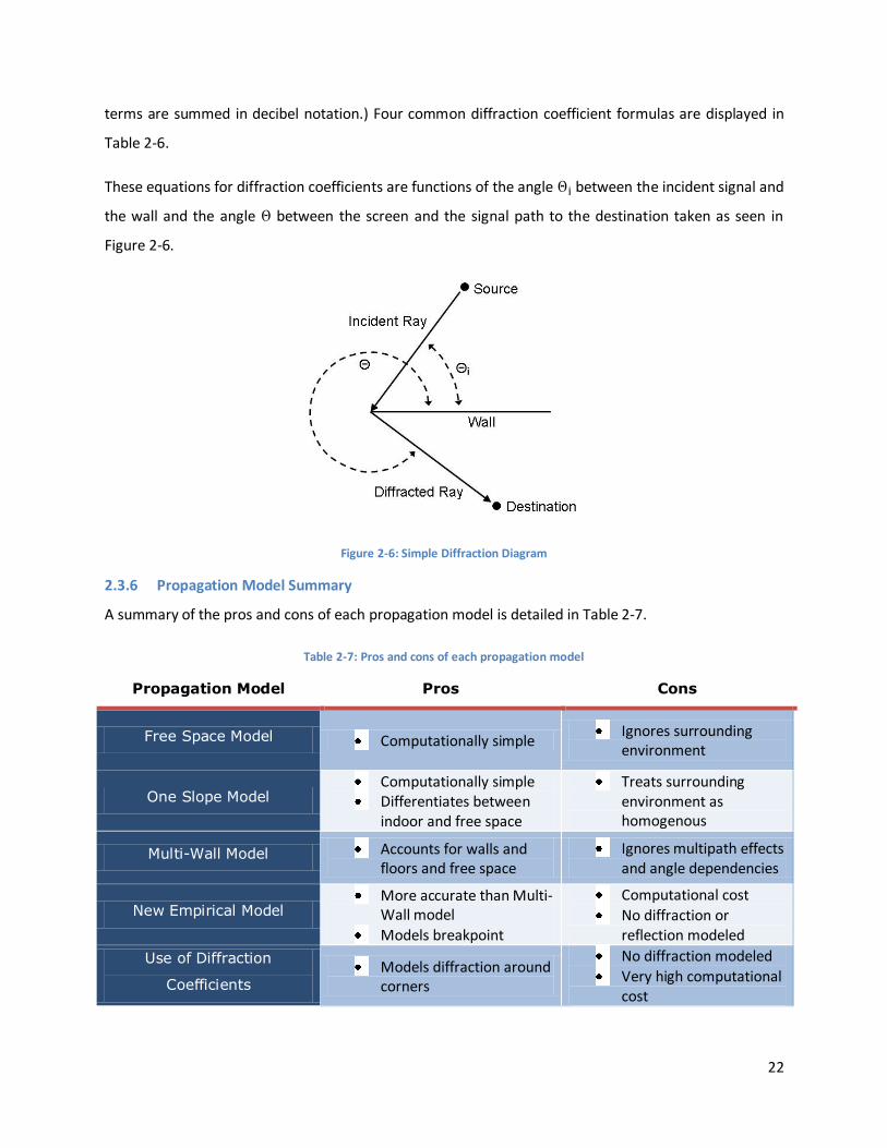
terms are summed in decibel notation.) Four common diffraction coefficient formulas are displayed in
Table 2-6.
These equations for diffraction coefficients are functions of the angle between the incident signal and
the wall and the angle between the screen and the signal path to the destination taken as seen in
Figure 2-6.
Figure 2-6: Simple Diffraction Diagram
2.3.6 Propagation Model Summary
A summary of the pros and cons of each propagation model is detailed in Table 2-7.
Table 2-7: Pros and cons of each propagation model
Propagation Model Pros Cons
Free Space Model Computationally simple Ignores surrounding
environment
One Slope Model Computationally simple Differentiates between
indoor and free space
Treats surrounding environment as homogenous
Multi-Wall Model Accounts for walls and floors and free space
Ignores multipath effects and angle dependencies
New Empirical Model More accurate than Multi-
Wall model
Models breakpoint
Computational cost
No diffraction or reflection modeled
Use of Diffraction
Coefficients Models diffraction around
corners
No diffraction modeled
Very high computational cost
23
2.4 Inertial Navigation System
An Inertial Navigation System (INS) is a navigation system that estimates the devices current position
relative to the initial position by incorporating the acceleration, velocity, direction and initial position.
An INS system typically needs an accelerometer to measure motion, a gyroscope or similar sensing
devices to measure direction, and a computer to perform calculations. The position relative to initial
position can be calculated from the accelerometer measurements, which provides movement
information relative to a previous location. With the accelerometer alone, the system could detect
relative motion. The use of additional hardware such as a compass is necessary to tell the direction of
movement.
The output of the accelerometer is a measure of the acceleration in three dimensions; the velocity in an
inertial reference frame can be calculated by integrating the inertial acceleration over time. Then the
position can be deduced by integrating the velocity.
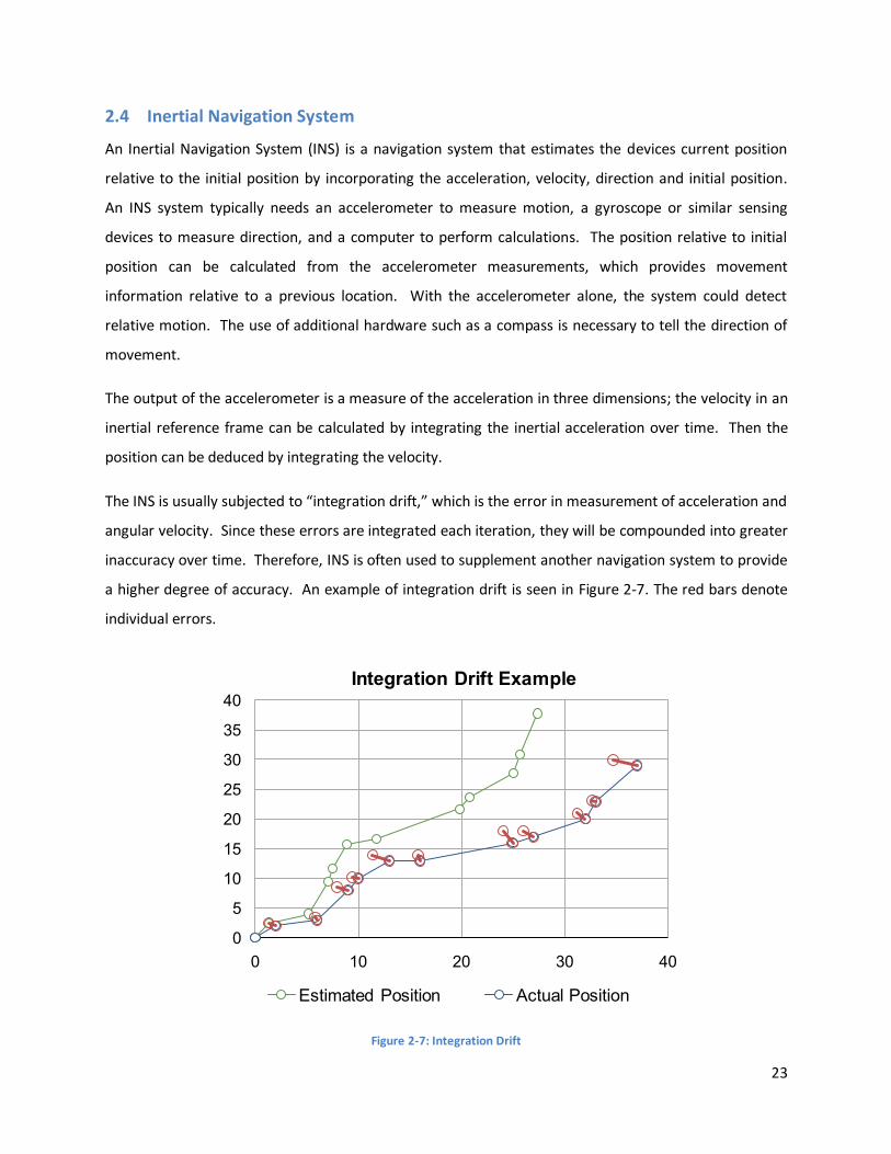
The INS is usually subjected to “integration drift,” which is the error in measurement of acceleration and
angular velocity. Since these errors are integrated each iteration, they will be compounded into greater
inaccuracy over time. Therefore, INS is often used to supplement another navigation system to provide
a higher degree of accuracy. An example of integration drift is seen in Figure 2-7. The red bars denote
individual errors.
Figure 2-7: Integration Drift
0
5
10
15
20
25
30
35
40
0 10 20 30 40
Integration Drift Example
Estimated Position Actual Position
24
2.4.1 Dead Reckoning
Dead Reckoning (DR) is the process used to estimate the position of an object relative to an initial
position, by calculating the current position from the estimated velocity, travel time and direction
course. Modern inertial navigation systems depend on DR in many applications, especially automated
vehicle applications.
A disadvantage of dead reckoning is that the errors could be potentially large due to its cumulative
nature. The reason is that the new position is estimated only from the knowledge of a correct previous
position; therefore any probability of error will grow exponentially over time. Another challenge of this
approach is that while it is used widely for inertial navigation systems, implementation on personal
device is difficult due to the low quality sensors available [12]. The sensor noise will blur the signal and
increase the potential error.
A method developed by the Geodetic Engineering Laboratory of EPFL utilizes a low cost inertial system
that detects human steps and identifies the step length based on biomechanical characteristic of the
step. The type of step can depend on different factors such as gender, age, height and weight of the
person. Their model is constructed and tested with blind people whose steps vary greatly depending on
familiarity with the area.
2.4.2 Map Matching
Map matching is a method for merging data from signal positioning and the digital map network to
estimate the location of the mobile object that best matches the digital map. The reason that such
techniques are necessary is that the location acquired from positioning techniques is subject to errors.
Map matching is often helpful when the position is expected to be on a certain path, such as in the
problem of tracking a moving vehicle on the route of GPS device.
Figure 2-8 provides a general system block diagram of a map matching process. The inputs of the
process are a digital map and positioning data. The digital map data is not a graphical picture
representation of an area but often in the form of a list of polylines in a graph [17]. The positioning
estimates are often not on the polyline provided, but scattered due to errors in the positioning system.
The map matching process will produce outputs that lay on the polyline. An example output is a GPS
device in a driving vehicle that matches the position of the car to the nearest road.

25
Figure 2-8: Using map matching to estimate the position of the device
There are two forms of map matching algorithms: online and offline. The online map matching
algorithm deals with situations in which only current and past data available to estimate the position
similar to the GPS device in a car. The offline map-matching algorithm is used when there is some or all
future data is available, such as a recorded track of a moving object.
The process of matching often involves three different phases: nomination, selection and calculation. In
the nomination phase, with the given positioning data, the algorithm will choose all the potential
polylines in the graph that the position could be on. The criterion for choosing a polyline is the normal
distance between the point and the polyline. If the distance is within the considered threshold, the
polyline will be chosen for the next step. The purpose of the nomination is to filter out all the polylines
that are too far away and unlikely to be the correct one. In the selection phase, a best polyline will be
chosen from the set of polylines filtered in the previous phase. This is the important part of the
algorithm to determine which one is the correct polyline. The criteria to consider can include last
positions, last correct polylines, estimation of future position, normal distance between the points and
the line. After a polyline is chosen, in the last phase, calculation, the estimated position on the polyline
of the point is computed and is given as the output of the process.
The error that is often exhibited in the map matching algorithm, specifically with online map matching,
is when the position is close to an intersection where the chosen polyline based on shortest distance
method may not be the correct polyline to map the mobile object to. This type of error is illustrated in
the Figure 2-9.

26
Figure 2-9: This picture shows possible errors in a map matching algorithm
In Figure 2-9, the green points represent the actual positioning data recorded from time zero from left
to right. The red point is the positioning data recorded that has received an incorrect map matching
estimation. The lines are the polylines in the graph that fall within the threshold range. The green line is
the polyline that has been chosen for previous positions. In this case, the map matching algorithm
mistakes the black line as the closest polyline to the red point. This would not be considered an error if
we do not know the next point, which for illustration purpose, is shown as the point on the right side of
the black line. When the position is close to an intersection, it will create an ambiguous situation where
the object could go straight or make a turn at the intersection. No correct position can be determined,
given the limited information available to the online map matching method for use in guaranteeing
which line the point should be on. However, for offline map matching with the information of future
points, we can safely deduct that the red point should be on the green line despite a closer distance to
the black line. Offline algorithm can provide a better estimation when future information is considered
with correction by combining previous and future matched points. This problem is inherent within
online map matching and can only be solved in offline map matching. A possible solution is to trade off
the responsiveness of the system with additional delay when considering future information, which can
minimize the error.
Yin and Wolfson propose a weighted-based offline map-matching algorithm [18]. Their approach is to
find the matched route so that the total distance between the matched route and real trajectory route
is the smallest. The weight is assigned to each edge on the graph using a 3 dimensional model by
combining two dimensional coordinates and time. The weight is be the integral of Euclidean distance
27
between the trajectory route and the matched route for the sub trajectory route during the interval
from ti to tj, divided by | tj - ti |.
There is a lot of research about map matching for navigation on roads with GPS. However, there is
limited research of the applicability of that algorithm for indoor navigation. These two environments
share the same nature. Therefore it is possible to use a similar approach for map matching in outdoor
environments and indoor navigation.
2.5 Mapping Techniques
Mapping a building involves gathering information that describes the building’s layout and converting
this information into a form that is usable by other processes. Types of data typically extracted include:
The location and size of walls, hallways, doors, floors, staircases, elevators, windows, etc.
Position of the map relative to other locations (latitude and longitude, elevation, floor number,
orientation)
The navigation process finds the shortest path from the current location determined by positioning
techniques to a desired destination within an unfamiliar area.
2.5.1 Mapping Information Formats
There are currently two common formats for building mapping information:
Two-dimensional map images are often posted to provide aid in navigation or to show fire
escape routes. The appearance of these maps varies depending on the software used to create
them or applicable building standards. The information that can be gathered from a map image
is primarily the floor plan of a building. The scale and coordination are generally not present,
but can be found in more technical maps such as printed blueprints.
Three-dimensional building models are available for structures constructed recently that were
designed with 3-D modeling utilities. This form of building mapping stores much more
information than the two dimensional images. Scale, Height, and connections to other floors
are all available. These models do not provide information regarding the location and
orientation of the building. The primary limitation of this file format as a resource is that it is
available for few buildings.
28
2.5.2 Map Creation Techniques
To make map images or models useful in software applications they are often converted into a new data
structure, which provides the necessary information in an accessible format. There are four aspects of
spatial relationship that a map data structure often needs to represent: connectivity, proximity,
intersection and membership. Different map data structures may focus on some aspects more than
others. In one example a map creation process was used to convert to a data structure composed of
points, arcs and polylines that represent different objects like rooms, doors, corridors, and stairs [12]. If
the raw data is a CAD file, the process is simpler because the structure has already been decomposed
into simple elements. Less complex processing techniques are necessary. If the map layout is in an
image format such as .jpg, .png, or .pdf the process of converting from raw data to a primitive data
structure requires the use of image processing techniques including object recognition and data
filtering. If a lower quality format is obtained (i.e. a photograph) further steps to correct skewed
perspectives or discoloring could be necessary.
2.5.3 Graphing Representation
In order to perform graphing algorithms to determine the shortest path between two locations, it is
necessary to convert the representation of a map data structure from layout with walls, halls, and doors
structure into nodes and links. In graphing representation, rooms, intersections, staircases, elevators
and other building units will be represented by nodes while the hallway will be represented by links that
connect between nodes. A node will also carry information related to the location including
coordination, and a link to a software database so that a user can get more information about the
person which the room belongs to. A link between two nodes represents an existing path in the building
where a person can walk between two locations directly. The assignment of the nodes is constructed so
that every link must be a straight line and represents the actual direct line of sight path. Curves and
turns will be represented by more than one link. The reason for this design is for the algorithm to
perform effectively. More information can be found in the system design chapter.
2.5.4 Routing Algorithm
Routing techniques use algorithms that find the shortest path between two locations. Typically a link
relationship between nodes in a graph will be represented by a two dimensional matrix. The
relationship between nodes is the weight or the cost of traveling from one to the other such as distance,
time, or degree of convenience. The relationship can also be represented by a list of edges. The choice
of data structure will affect the size of the database as well as the performance of the algorithm. Some
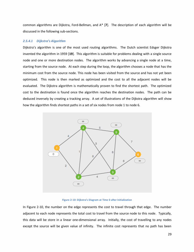
29
common algorithms are Dijkstra, Ford-Bellman, and A* [7]. The description of each algorithm will be
discussed in the following sub-sections.
2.5.4.1 Dijkstra’s Algorithm
Dijkstra’s algorithm is one of the most used routing algorithms. The Dutch scientist Edsger Dijkstra
invented the algorithm in 1959 [19]. This algorithm is suitable for problems dealing with a single source
node and one or more destination nodes. The algorithm works by advancing a single node at a time,
starting from the source node. At each step during the loop, the algorithm chooses a node that has the
minimum cost from the source node. This node has been visited from the source and has not yet been
optimized. This node is then marked as optimized and the cost to all the adjacent nodes will be
evaluated. The Dijkstra algorithm is mathematically proven to find the shortest path. The optimized
cost to the destination is found once the algorithm reaches the destination nodes. The path can be
deduced inversely by creating a tracking array. A set of illustrations of the Dijkstra algorithm will show
how the algorithm finds shortest paths in a set of six nodes from node 1 to node 6.
Figure 2-10: Dijkstra’s Diagram at Time 0 after Initialization
In Figure 2-10, the number on the edge represents the cost to travel through that edge. The number
adjacent to each node represents the total cost to travel from the source node to this node. Typically,
this data will be store in a linear one-dimensional array. Initially, the cost of travelling to any nodes
except the source will be given value of infinity. The infinite cost represents that no path has been
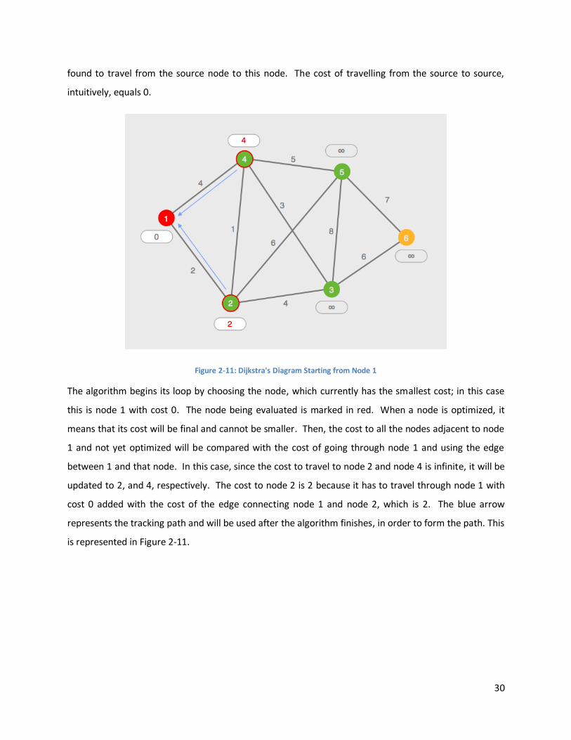
30
found to travel from the source node to this node. The cost of travelling from the source to source,
intuitively, equals 0.
Figure 2-11: Dijkstra's Diagram Starting from Node 1
The algorithm begins its loop by choosing the node, which currently has the smallest cost; in this case
this is node 1 with cost 0. The node being evaluated is marked in red. When a node is optimized, it
means that its cost will be final and cannot be smaller. Then, the cost to all the nodes adjacent to node
1 and not yet optimized will be compared with the cost of going through node 1 and using the edge
between 1 and that node. In this case, since the cost to travel to node 2 and node 4 is infinite, it will be
updated to 2, and 4, respectively. The cost to node 2 is 2 because it has to travel through node 1 with
cost 0 added with the cost of the edge connecting node 1 and node 2, which is 2. The blue arrow
represents the tracking path and will be used after the algorithm finishes, in order to form the path. This
is represented in Figure 2-11.
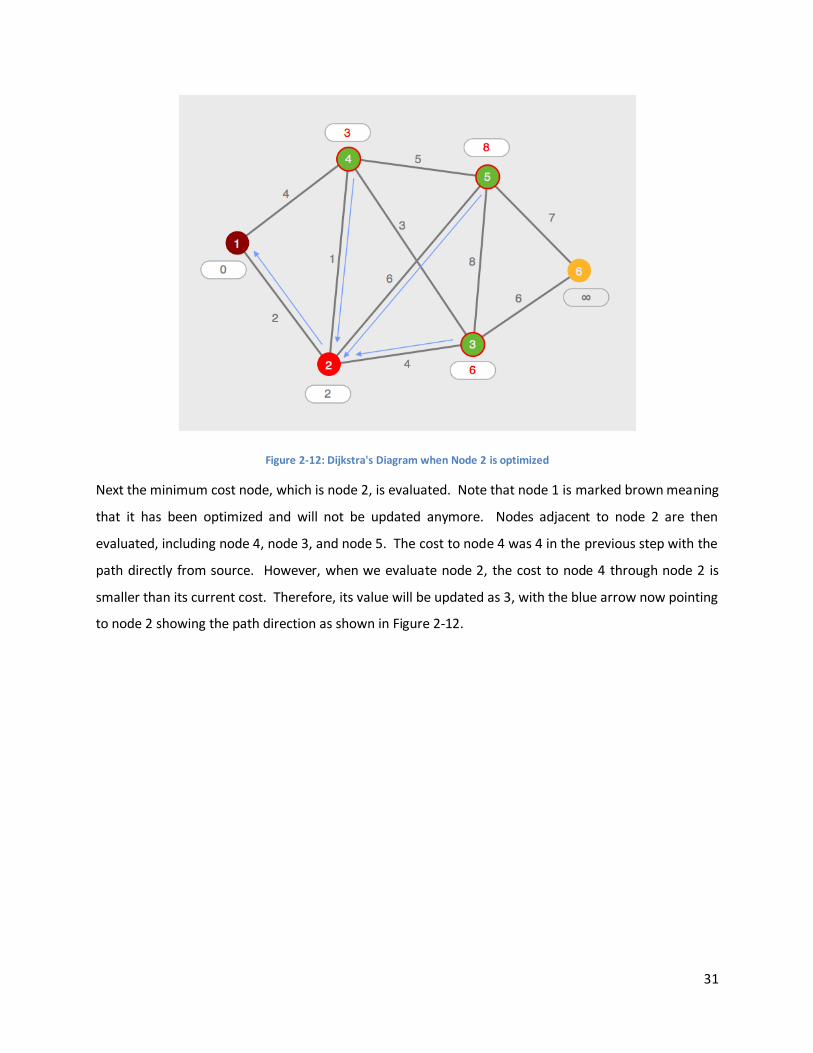
31
Figure 2-12: Dijkstra's Diagram when Node 2 is optimized
Next the minimum cost node, which is node 2, is evaluated. Note that node 1 is marked brown meaning
that it has been optimized and will not be updated anymore. Nodes adjacent to node 2 are then
evaluated, including node 4, node 3, and node 5. The cost to node 4 was 4 in the previous step with the
path directly from source. However, when we evaluate node 2, the cost to node 4 through node 2 is
smaller than its current cost. Therefore, its value will be updated as 3, with the blue arrow now pointing
to node 2 showing the path direction as shown in Figure 2-12.
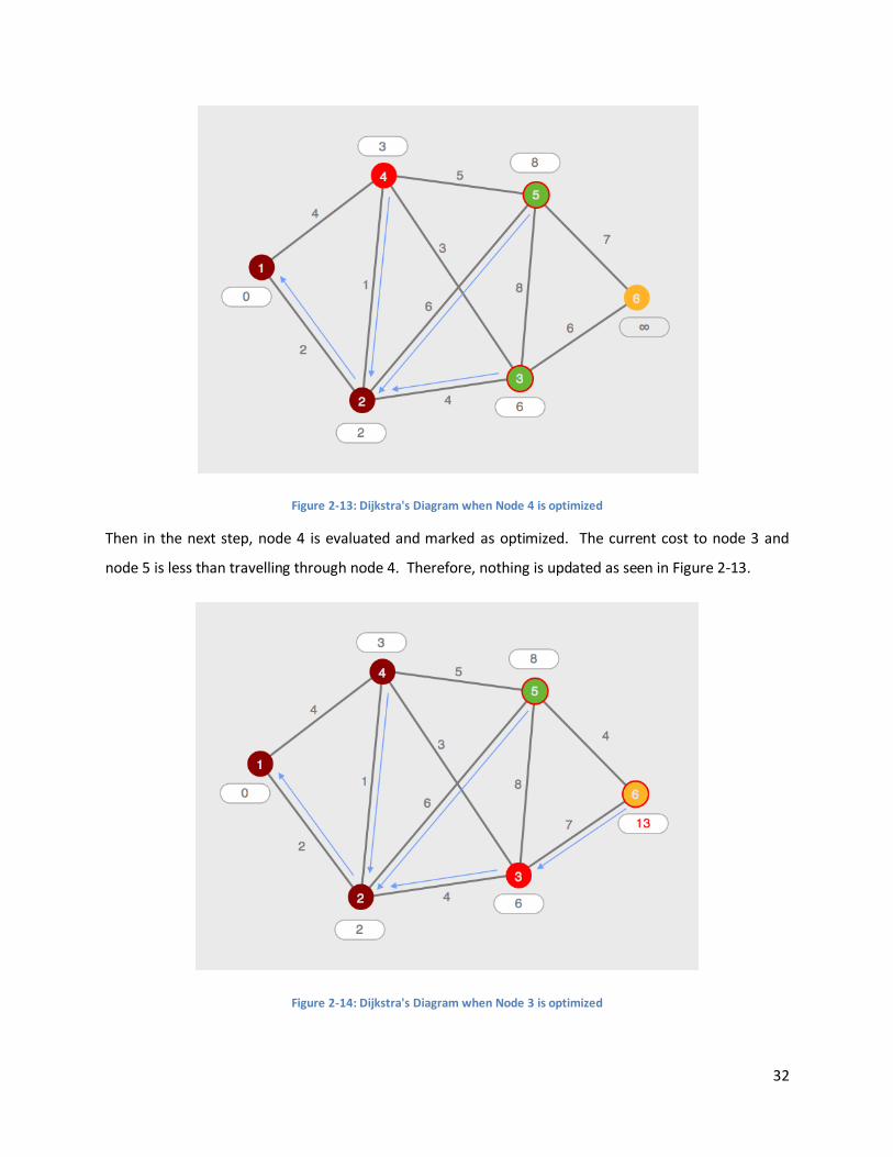
32
Figure 2-13: Dijkstra's Diagram when Node 4 is optimized
Then in the next step, node 4 is evaluated and marked as optimized. The current cost to node 3 and
node 5 is less than travelling through node 4. Therefore, nothing is updated as seen in Figure 2-13.
Figure 2-14: Dijkstra's Diagram when Node 3 is optimized
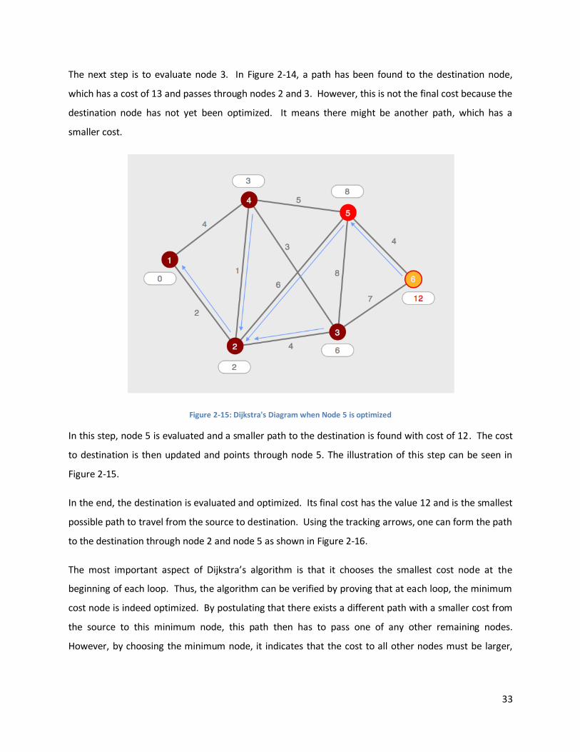
33
The next step is to evaluate node 3. In Figure 2-14, a path has been found to the destination node,
which has a cost of 13 and passes through nodes 2 and 3. However, this is not the final cost because the
destination node has not yet been optimized. It means there might be another path, which has a
smaller cost.
Figure 2-15: Dijkstra's Diagram when Node 5 is optimized
In this step, node 5 is evaluated and a smaller path to the destination is found with cost of 12. The cost
to destination is then updated and points through node 5. The illustration of this step can be seen in
Figure 2-15.
In the end, the destination is evaluated and optimized. Its final cost has the value 12 and is the smallest
possible path to travel from the source to destination. Using the tracking arrows, one can form the path
to the destination through node 2 and node 5 as shown in Figure 2-16.
The most important aspect of Dijkstra’s algorithm is that it chooses the smallest cost node at the
beginning of each loop. Thus, the algorithm can be verified by proving that at each loop, the minimum
cost node is indeed optimized. By postulating that there exists a different path with a smaller cost from
the source to this minimum node, this path then has to pass one of any other remaining nodes.
However, by choosing the minimum node, it indicates that the cost to all other nodes must be larger,
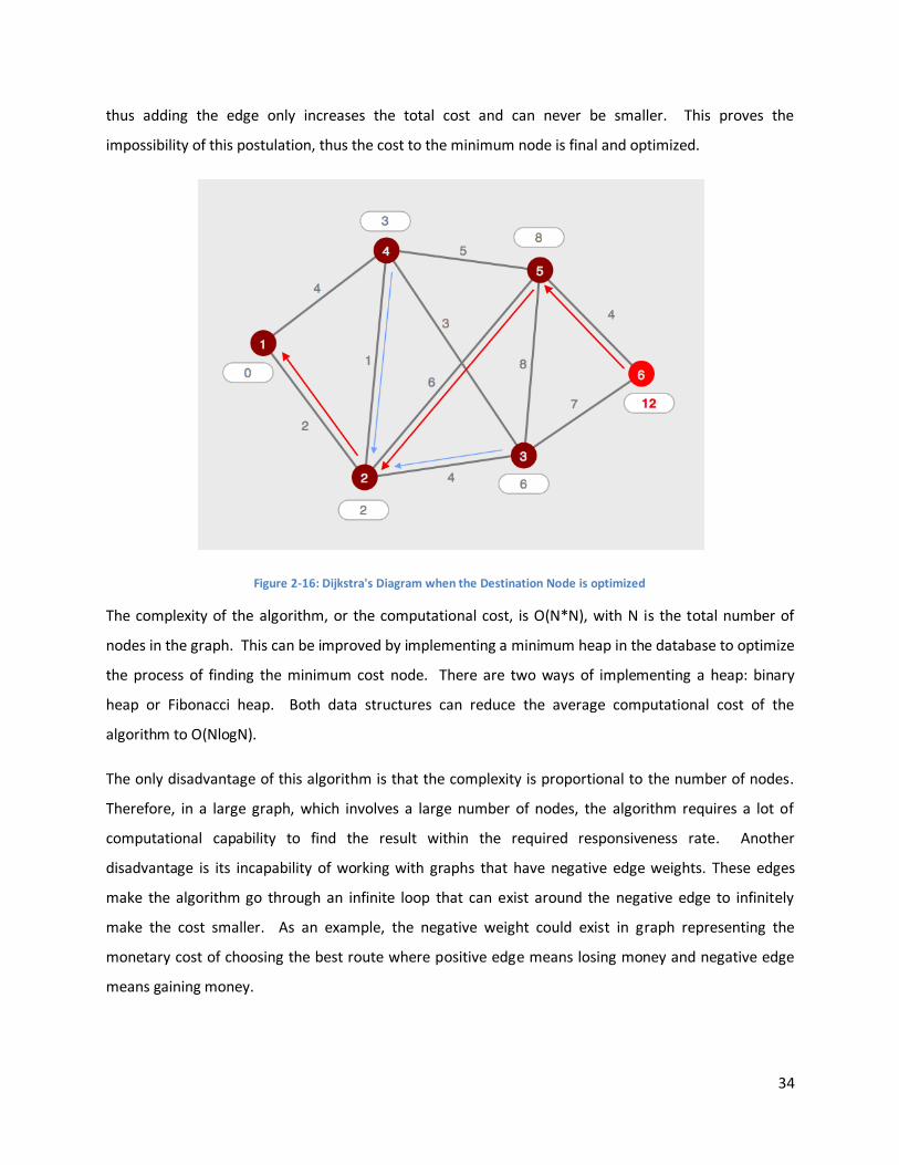
34
thus adding the edge only increases the total cost and can never be smaller. This proves the
impossibility of this postulation, thus the cost to the minimum node is final and optimized.
Figure 2-16: Dijkstra's Diagram when the Destination Node is optimized
The complexity of the algorithm, or the computational cost, is O(N*N), with N is the total number of
nodes in the graph. This can be improved by implementing a minimum heap in the database to optimize
the process of finding the minimum cost node. There are two ways of implementing a heap: binary
heap or Fibonacci heap. Both data structures can reduce the average computational cost of the
algorithm to O(NlogN).
The only disadvantage of this algorithm is that the complexity is proportional to the number of nodes.
Therefore, in a large graph, which involves a large number of nodes, the algorithm requires a lot of
computational capability to find the result within the required responsiveness rate. Another
disadvantage is its incapability of working with graphs that have negative edge weights. These edges
make the algorithm go through an infinite loop that can exist around the negative edge to infinitely
make the cost smaller. As an example, the negative weight could exist in graph representing the
monetary cost of choosing the best route where positive edge means losing money and negative edge
means gaining money.
35
2.5.4.2 Bellman-Ford Algorithm
The Bellman-Ford algorithm is specifically designed to solve the problem of finding the shortest path in a
graph containing negative weight edges [7]. It addresses the incapability of Dijkstra to work with
negative edges by adding a protection that prevents the path from passing through a negative cycle.
Instead of choosing the minimum cost node at each loop and updating all of its adjacent nodes as in
Dijkstra’s algorithm, the Bellman-Ford algorithm updates all possible edges existing in the graph. This
prevents the algorithm from choosing the same minimum node infinitely. The amount of updating time
in the algorithm is equivalent to the maximum length of the shortest path to be considered. By
updating n times, which is the number of the vertices in the graph, the algorithm can find the optimal
solution. While the Bellman-Ford algorithm can work with weighted graphs, its running time is worse
than the Dijkstra algorithm because it has to update all possible edges in the graph instead of just edges
adjacent to the minimum cost node. Therefore, it increases the total complexity of the algorithm to
O(N3). Because of its high complexity, Bellman-Ford should only be used when the graph contains
negative weight edges.
2.5.4.3 A* Algorithm
The A*, or A star, algorithm is a different algorithm to solve the problem of finding the shortest path
between two nodes in a graph [7]. Similar in concept to Dijkstra’s algorithm, it finds the shortest path
by advancing one node at a time from the source. The difference between the A* algorithm and Dijkstra
algorithm is in its shortest path formula and its updating process. Instead of updating all the adjacent
nodes, the A* algorithm only updates nodes that have not been visited before with an optimistic hope
that this is the shortest path because it comes from the shortest “estimated path”. The shortest path in
the A* at each step is not absolute. Instead it is a sum of the absolute path from the source to the node
and a heuristic estimation of the distance from this node to the destination. The optimal performance
of the A* algorithm depends on the heuristic model. The heuristic estimation has to be reasonable, and
should not overestimate the distance between the node and the destination. The heuristic formula of
the distance between the node and the destination must satisfy the condition that there is no path in
the graph that could be smaller than the heuristic estimation. However it should not overestimate the
distance by assigning a very small value, which affects the process of choosing the minimum node. For
example, a good heuristic model can be developed when the graph is in Earth coordinates. The heuristic
model can be natively computed as the Euclidean distance between two coordinates. Although the A*
algorithm provides a lower complexity cost than Dijkstra algorithm, the solution determined by this
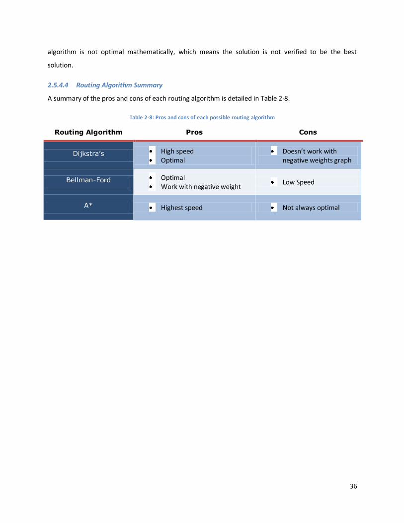
36
algorithm is not optimal mathematically, which means the solution is not verified to be the best
solution.
2.5.4.4 Routing Algorithm Summary
A summary of the pros and cons of each routing algorithm is detailed in Table 2-8.
Table 2-8: Pros and cons of each possible routing algorithm
Routing Algorithm Pros Cons
Dijkstra’s High speed Optimal
Doesn’t work with negative weights graph
Bellman-Ford Optimal Work with negative weight
Low Speed
A* Highest speed Not always optimal
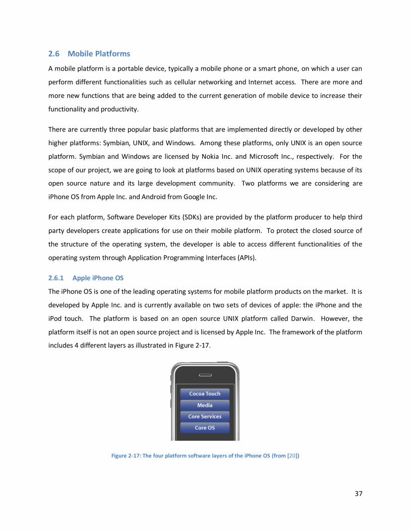
37
2.6 Mobile Platforms
A mobile platform is a portable device, typically a mobile phone or a smart phone, on which a user can
perform different functionalities such as cellular networking and Internet access. There are more and
more new functions that are being added to the current generation of mobile device to increase their
functionality and productivity.
There are currently three popular basic platforms that are implemented directly or developed by other
higher platforms: Symbian, UNIX, and Windows. Among these platforms, only UNIX is an open source
platform. Symbian and Windows are licensed by Nokia Inc. and Microsoft Inc., respectively. For the
scope of our project, we are going to look at platforms based on UNIX operating systems because of its
open source nature and its large development community. Two platforms we are considering are
iPhone OS from Apple Inc. and Android from Google Inc.
For each platform, Software Developer Kits (SDKs) are provided by the platform producer to help third
party developers create applications for use on their mobile platform. To protect the closed source of
the structure of the operating system, the developer is able to access different functionalities of the
operating system through Application Programming Interfaces (APIs).
2.6.1 Apple iPhone OS
The iPhone OS is one of the leading operating systems for mobile platform products on the market. It is
developed by Apple Inc. and is currently available on two sets of devices of apple: the iPhone and the
iPod touch. The platform is based on an open source UNIX platform called Darwin. However, the
platform itself is not an open source project and is licensed by Apple Inc. The framework of the platform
includes 4 different layers as illustrated in Figure 2-17.
Figure 2-17: The four platform software layers of the iPhone OS (from [20])
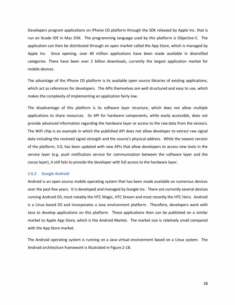
38
Developers program applications on iPhone OS platform through the SDK released by Apple Inc. that is
run on Xcode IDE in Mac OSX. The programming language used by this platform is Objective-C. The
application can then be distributed through an open market called the App Store, which is managed by
Apple Inc. Since opening, over 40 million applications have been made available in diversified
categories. There have been over 2 billion downloads, currently the largest application market for
mobile devices.
The advantage of the iPhone OS platform is its available open source libraries of existing applications,
which act as references for developers. The APIs themselves are well structured and easy to use, which
makes the complexity of implementing an application fairly low.
The disadvantage of this platform is its software layer structure, which does not allow multiple
applications to share resources. Its API for hardware components, while easily accessible, does not
provide advanced information regarding the hardware layer or access to the raw data from the sensors.
The WiFi chip is an example in which the published API does not allow developer to extract raw signal
data including the received signal strength and the source’s physical address. While the newest version
of the platform, 3.0, has been updated with new APIs that allow developers to access new tools in the
service layer (e.g. push notification service for communication between the software layer and the
cocoa layer), it still fails to provide the developer with full access to the hardware layer.
2.6.2 Google Android
Android is an open source mobile operating system that has been made available on numerous devices
over the past few years. It is developed and managed by Google Inc. There are currently several devices
running Android OS, most notably the HTC Magic, HTC Dream and most recently the HTC Hero. Android
is a Linux based OS and incorporates a Java environment platform. Therefore, developers work with
Java to develop applications on this platform. These applications then can be published on a similar
market to Apple App Store, which is the Android Market. The market size is relatively small compared
with the App Store market.
The Android operating system is running on a Java virtual environment based on a Linux system. The
Android architecture framework is illustrated in Figure 2-18.

39
Figure 2-18: Google Android Operating System Architecture Framework (from [21])
The advantage of Android is that it is open source and it provides full accessibility to many hardware
layers. Moreover, the operating system structure allows developer to easily access the core services of
the platform as well as channel information between applications, which is not possible under the
iPhone OS platform.
The disadvantage of this platform is that there are currently not many users as well as few developers.
This limits the potential for implementation on a larger scale. However, the platform is expected to gain
popularity in the near future as more mobile devices are currently being developed for this platform.
2.6.3 Mobile Platform Summary
Consumer popularity indicates how many available devices on the market are using each platform. This
is important because it affects how well the final application can reach customers and how easily it can
be implemented and distributed. According to an industry study in June 2009 by Flurry Inc. (Figure
2-19), the consumer usage for the mobile platform is [22]:
40
Figure 2-19: Consumer Popularity of Mobile Platform in July 2009
While it is clearly shows that the iPhone is the leader in terms of popularity and Android’s share is
relatively small, we should be aware that the Android is still new to the market, and one year younger
than the iPhone, with its first product released November 2008.
Developer popularity indicates the number of developers that are currently researching and developing
applications for each platform. While this does not contribute to the end usage side, it directly affects
our application because of the open source nature of Google Android, where developers could share
resources and experiences. Higher the developer popularity indicates faster implementation potential.
It also shows that it is more likely that future improvement could occur.
As seen in Figure 2-20, the 22% share of developers who use Android indicates that while this platform
is relatively new, there are more developers seeing the potential performance of this platform. It
indicates that new mobile devices will be improved to exploit the potential of this platform.
iPhone91%
Android7%
Others2%
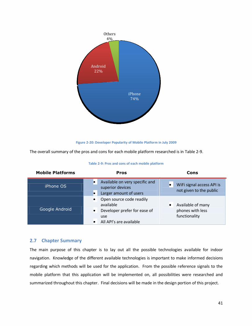
41
Figure 2-20: Developer Popularity of Mobile Platform in July 2009
The overall summary of the pros and cons for each mobile platform researched is in Table 2-9.
Table 2-9: Pros and cons of each mobile platform
Mobile Platforms Pros Cons
iPhone OS Available on very specific and
superior devices
Larger amount of users
WiFi signal access API is not given to the public
Google Android
Open source code readily available
Developer prefer for ease of use
All API’s are available
Available of many phones with less functionality
2.7 Chapter Summary
The main purpose of this chapter is to lay out all the possible technologies available for indoor
navigation. Knowledge of the different available technologies is important to make informed decisions
regarding which methods will be used for the application. From the possible reference signals to the
mobile platform that this application will be implemented on, all possibilities were researched and
summarized throughout this chapter. Final decisions will be made in the design portion of this project.
iPhone74%
Android22%
Others4%

42
3 Project Overview and Design
This chapter presents the project overview, which contains the goals and objectives of the project, as
well as the general design of the system.
3.1 Goal
The main goal of this system is to facilitate indoor navigation for able-bodied and impaired persons. In
the intended application, handheld devices will be given the capability to guide a person along the most
desirable path to their selected destination. The system will be easy to implement in buildings that have
existing wireless connectivity.
3.2 Objectives
To function as intended, the system must meet three primary objectives:
The device must be able to accurately determine its location in a building
The device must guide a user along an optimal path to their destination
The device must have an intuitive user interface
These objectives will be accomplished through the design and integration of a number of subsystems.
The first objective is to be able to locate the handheld device in a building. The device should be able to
use signal strength measurements of the available wireless networks to accurately locate itself in a
building. The device should be able to look up its exact location in relation to the map according to the
wireless propagation model.
The second objective is to use routing algorithms to be able to lead the user to their final destination by
finding the shortest possible route and leading the user along it. Finding the optimal algorithm for
determining the correct path with a minimum requirement for computing resources is necessary.
The third and final objective is to create a user interface that is intuitive. The user should be able to look
up a desired destination and the device should be able to show the user a route to it. A database of
possible destinations should be provided. In the building that we will be testing this application in, the
device should support searching of the database by multiple parameters.
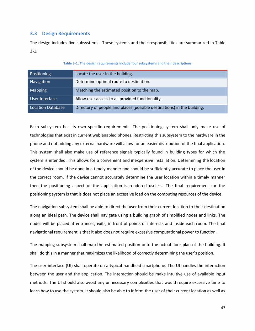
43
3.3 Design Requirements
The design includes five subsystems. These systems and their responsibilities are summarized in Table
3-1.
Table 3-1: The design requirements include four subsystems and their descriptions
Positioning Locate the user in the building.
Navigation Determine optimal route to destination.
Mapping Matching the estimated position to the map.
User Interface Allow user access to all provided functionality.
Location Database Directory of people and places (possible destinations) in the building.
Each subsystem has its own specific requirements. The positioning system shall only make use of
technologies that exist in current web enabled phones. Restricting this subsystem to the hardware in the
phone and not adding any external hardware will allow for an easier distribution of the final application.
This system shall also make use of reference signals typically found in building types for which the
system is intended. This allows for a convenient and inexpensive installation. Determining the location
of the device should be done in a timely manner and should be sufficiently accurate to place the user in
the correct room. If the device cannot accurately determine the user location within a timely manner
then the positioning aspect of the application is rendered useless. The final requirement for the
positioning system is that is does not place an excessive load on the computing resources of the device.
The navigation subsystem shall be able to direct the user from their current location to their destination
along an ideal path. The device shall navigate using a building graph of simplified nodes and links. The
nodes will be placed at entrances, exits, in front of points of interests and inside each room. The final
navigational requirement is that it also does not require excessive computational power to function.
The mapping subsystem shall map the estimated position onto the actual floor plan of the building. It
shall do this in a manner that maximizes the likelihood of correctly determining the user’s position.
The user interface (UI) shall operate on a typical handheld smartphone. The UI handles the interaction
between the user and the application. The interaction should be make intuitive use of available input
methods. The UI should also avoid any unnecessary complexities that would require excessive time to
learn how to use the system. It should also be able to inform the user of their current location as well as
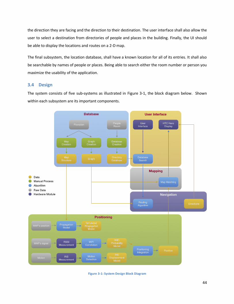
44
the direction they are facing and the direction to their destination. The user interface shall also allow the
user to select a destination from directories of people and places in the building. Finally, the UI should
be able to display the locations and routes on a 2-D map.
The final subsystem, the location database, shall have a known location for all of its entries. It shall also
be searchable by names of people or places. Being able to search either the room number or person you
maximize the usability of the application.
3.4 Design
The system consists of five sub-systems as illustrated in Figure 3-1, the block diagram below. Shown
within each subsystem are its important components.
Figure 3-1: System Design Block Diagram
45
The database block takes information about the local environment and provides it in a format that can
be used by other subsystems. The map floor plan is used to create the building walls structure that is
necessary for creation of the propagation model. The map floor plan is also used to create a graph
system to use in the routing algorithm.
Displaying the information including the map of the building, current location and the directions to get
to the destination is in the User Interface subsystem. It also handles interactions between the user and
the system. The database and user interface subsystem will be mention in Chapter 6.
The hardware layer consists of sensors in the HTC Hero. These include: the WiFi chipset, the
accelerometer and the magnetic compass. Raw data from these sensors is converted into useful
information, and processed by the positioning subsystem.
In the positioning layer, two methods are used in conjunction with one another in order to determine
the devices position: WiFi positioning and the Inertial Navigation System (INS). The WiFi positioning
system correlates measured WiFi signal strengths to a pre-generated database of simulated signal
strengths values for WAPs that are known to be in the area. The database is generated using a simulated
propagation model that models the signal strength from the building structure and the location of the
Wireless Access Points inside the building. The INS method determines the relative change in position by
accumulating measurements of the devices motion. Information from these two systems is combined in
order to provide an accurate approximation of the devices position. This information is then matched to
the map of the building in order to facilitate calculation of a route to the user’s final destination. The
positioning subsystem is described in Chapter 4. The Navigation and mapping subsystem, which handles
routing algorithm and map matching algorithm are described in Chapter 5.
3.5 Positioning Techniques
Following consideration of the positioning techniques identified during background research and of the
capabilities of handheld devices, the choice was made to use a combination of two techniques to
determine position.
An RF positioning technique similar to location fingerprinting will be used to determine location based
on received signal strengths from WAPs in the building. This system will use a propagation model to
create a database of simulate RSSI fingerprints. The use of a model makes the large amount of empirical
data typically associated with fingerprinting unnecessary.
46
An Inertial navigation system will be used to detect changes in position. By measuring the devices
acceleration and orientation in three dimensions, an estimate of changes in velocity and displacement
can be obtained. This type of positioning system relies on periodic updates of absolute position in order
to correct errors that accumulate in its estimate of relative position.
3.6 Mobile Platform
Of the two platforms that we have considered, Apple iPhone OS and Google Android, each has strengths
in different areas. While each area is weighted differently according to the scope of our research and its
importance to the final application, we must choose the best possible platform.
The most important factor is the technical specifications. The platform must have the capabilities
required for our application. The platform must support accessibility to the hardware that is used for
our project such as the WiFi hardware chipset and the accelerometer. Also, the accuracy of the chipset
and the sample rate are big contributing factor.
The overall usage of each platform is also an important factor. As seen in Figure 2-19 the consumer
popularity is extremely high for the Apple iPhone while the Google Android is significantly lower.
However, in Figure 2-20 it is seen that the developer popularity has a much larger proportion, even
though it is not close to the majority, which shows a potential for future growth.
The biggest drawback that makes the iPhone platform undesirable is that the iPhone API’s do not
provide full accessibility to the WiFi chipset to return the raw data of a wireless scan including the
Received Signal Strength Indicator (RSSI). This immediately makes the iPhone platform unusable for the
scope of our project. However, if future iPhone OS support this requirement, it would be another
option that should be fully explored to migrate the system from Android to the iPhone OS due to the
large market share and developers.
Therefore, the Android is the platform chosen for our project. We chose the newest mobile device
running Android to implement our prototype: the HTC Hero. The HTC Hero is developed by HTC Inc. and
runs Android as its core operating system with additional functionality. The specifications of the HTC
Hero are shown in Table 3-2 below.
3.7 Summary
Three primary objectives were identified that the system must meet; it must locate the user, determine
a route to the user’s destination, and interface with the user in an intuitive way. To meet these
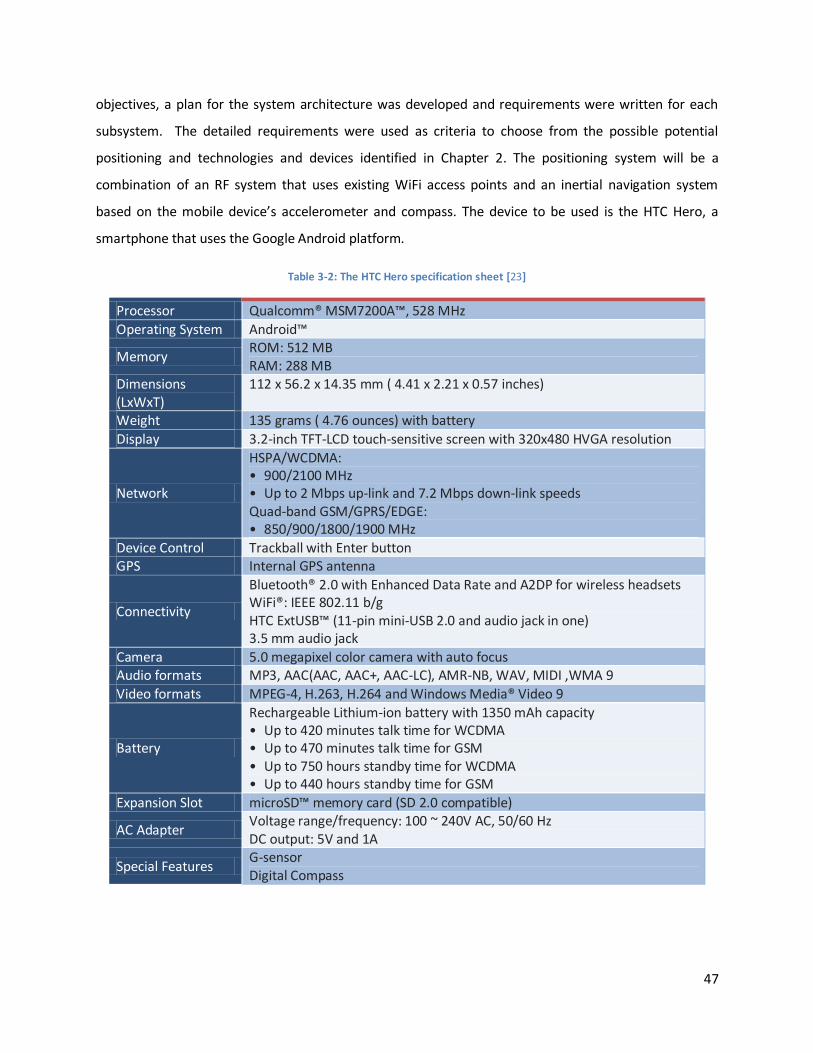
47
objectives, a plan for the system architecture was developed and requirements were written for each
subsystem. The detailed requirements were used as criteria to choose from the possible potential
positioning and technologies and devices identified in Chapter 2. The positioning system will be a
combination of an RF system that uses existing WiFi access points and an inertial navigation system
based on the mobile device’s accelerometer and compass. The device to be used is the HTC Hero, a
smartphone that uses the Google Android platform.
Table 3-2: The HTC Hero specification sheet [23]
Processor Qualcomm® MSM7200A™, 528 MHz
Operating System Android™
Memory ROM: 512 MB RAM: 288 MB
Dimensions (LxWxT)
112 x 56.2 x 14.35 mm ( 4.41 x 2.21 x 0.57 inches)
Weight 135 grams ( 4.76 ounces) with battery
Display 3.2-inch TFT-LCD touch-sensitive screen with 320x480 HVGA resolution
Network
HSPA/WCDMA: • 900/2100 MHz • Up to 2 Mbps up-link and 7.2 Mbps down-link speeds Quad-band GSM/GPRS/EDGE: • 850/900/1800/1900 MHz
Device Control Trackball with Enter button GPS Internal GPS antenna
Connectivity
Bluetooth® 2.0 with Enhanced Data Rate and A2DP for wireless headsets WiFi®: IEEE 802.11 b/g HTC ExtUSB™ (11-pin mini-USB 2.0 and audio jack in one) 3.5 mm audio jack
Camera 5.0 megapixel color camera with auto focus Audio formats MP3, AAC(AAC, AAC+, AAC-LC), AMR-NB, WAV, MIDI ,WMA 9
Video formats MPEG-4, H.263, H.264 and Windows Media® Video 9
Battery
Rechargeable Lithium-ion battery with 1350 mAh capacity • Up to 420 minutes talk time for WCDMA • Up to 470 minutes talk time for GSM • Up to 750 hours standby time for WCDMA • Up to 440 hours standby time for GSM
Expansion Slot microSD™ memory card (SD 2.0 compatible)
AC Adapter Voltage range/frequency: 100 ~ 240V AC, 50/60 Hz DC output: 5V and 1A
Special Features G-sensor Digital Compass
48
4 Positioning
The capability to determine a user’s position within a building is a necessary part of a navigation system.
The system described in this project uses measurements from WiFi, magnetic, and acceleration sensors
to estimate the user’s position. In this chapter the WiFi positioning subsystem is presented first,
followed by the inertial navigation system consisting of the acceleration and magnetic sensors. The last
section describes the technique that is used to combine the information from these two systems in
order to produce a continuous position estimate.
4.1 WiFi Positioning
The WiFi positioning system consists of two primary subsystems, the propagation model and the
location search algorithm. The propagation model is run on a computer and is used to pre-generate an
estimate of wireless signal strengths at each location. The location search algorithm combines
information from all detected wireless access points in order to determine the likelihood of the device
receiving a set of measurements at various locations in the building. This search function is
implemented on the mobile device.
4.1.1 Propagation Model
From the list of potential propagation models identified in Section 2.3, the pros and cons of each were
weighed and it was determined that the New Empirical model [14] would be used in combination with
the KED Screen diffraction model [16]. Due to the fact that propagation simulations are carried out in
advance, the high computational costs of the New Empirical model were deemed to be acceptable. For
an explanation of these models, consult Section 2.3.
The mathematical propagation and diffraction models were used to create a propagation simulation in
MATLAB. As inputs, this simulation requires a list of wall elements that define the building layout, as
well as the location and power of a wireless access point. The output is a .txt file that is transferred to
the HTC hero. To accelerate computations, the calculations were carried out using array operations
available in MATLAB. Figure 4-1 shows a top level flowchart of the simulation. Operations highlighted in
blue are array operations that would typically be implemented as loops in other programming
languages. The lowest blue operation is a loop in which each execution consists of a set of array
operations. With the propagation losses simulated, the estimate of received signal strength can be
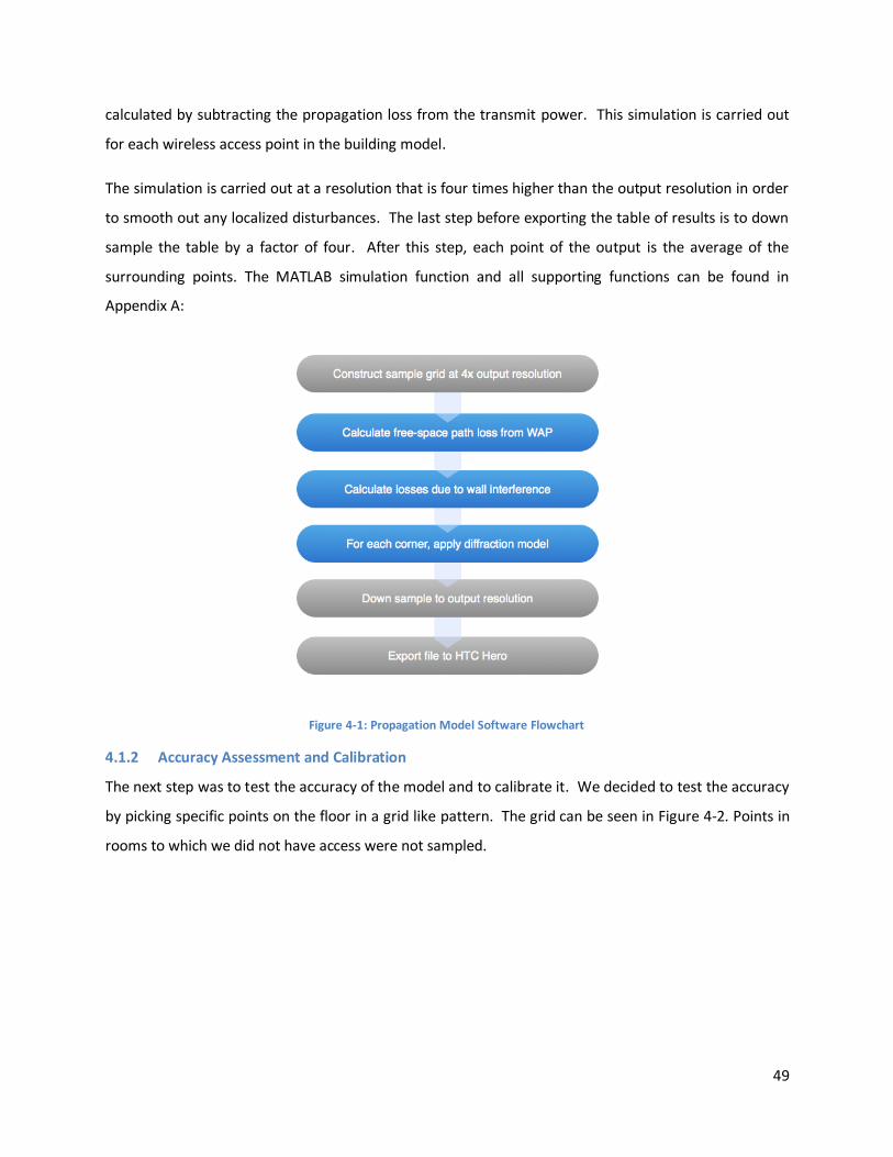
49
calculated by subtracting the propagation loss from the transmit power. This simulation is carried out
for each wireless access point in the building model.
The simulation is carried out at a resolution that is four times higher than the output resolution in order
to smooth out any localized disturbances. The last step before exporting the table of results is to down
sample the table by a factor of four. After this step, each point of the output is the average of the
surrounding points. The MATLAB simulation function and all supporting functions can be found in
Appendix A:
Figure 4-1: Propagation Model Software Flowchart
4.1.2 Accuracy Assessment and Calibration
The next step was to test the accuracy of the model and to calibrate it. We decided to test the accuracy
by picking specific points on the floor in a grid like pattern. The grid can be seen in Figure 4-2. Points in
rooms to which we did not have access were not sampled.
50
Figure 4-2: Accuracy Testing Points
4.1.2.1 Single WAP Laptop-Based Propagation Model Test
The first test was conducted using a laptop to test RSSI values at each location. The first test yielded the
following results.
Figure 4-3: Test Results Showing Moderate Correlation between Measured and Predicted Values
The results show an R2 value of .725, which can be interpreted as a moderate correlation between
predicted and measured values. Using this information, unknown transmit powers of the WAPs were
determined.
y = 1.1034x - 6.9612R² = 0.7246
40
50
60
70
80
90
100
40 50 60 70 80 90 100
Pre
dic
ted
Va
lue
Measured Value
Propagation Model Accuracy
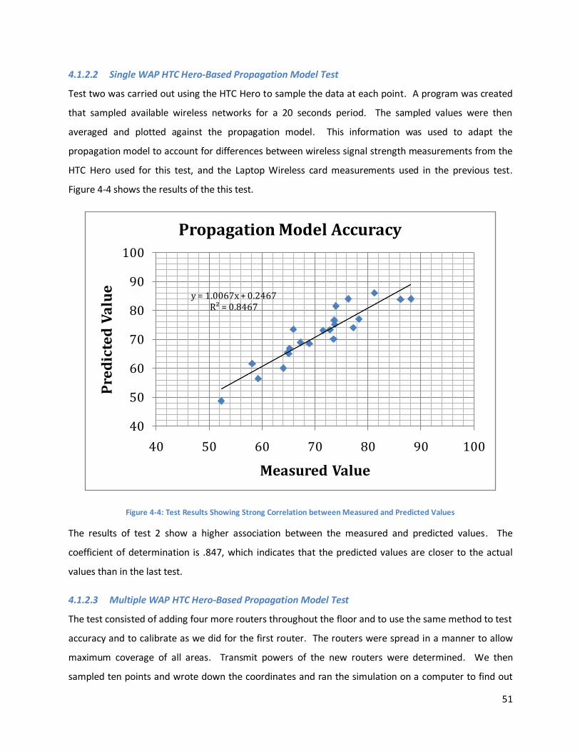
51
4.1.2.2 Single WAP HTC Hero-Based Propagation Model Test
Test two was carried out using the HTC Hero to sample the data at each point. A program was created
that sampled available wireless networks for a 20 seconds period. The sampled values were then
averaged and plotted against the propagation model. This information was used to adapt the
propagation model to account for differences between wireless signal strength measurements from the
HTC Hero used for this test, and the Laptop Wireless card measurements used in the previous test.
Figure 4-4 shows the results of the this test.
Figure 4-4: Test Results Showing Strong Correlation between Measured and Predicted Values
The results of test 2 show a higher association between the measured and predicted values. The
coefficient of determination is .847, which indicates that the predicted values are closer to the actual
values than in the last test.
4.1.2.3 Multiple WAP HTC Hero-Based Propagation Model Test
The test consisted of adding four more routers throughout the floor and to use the same method to test
accuracy and to calibrate as we did for the first router. The routers were spread in a manner to allow
maximum coverage of all areas. Transmit powers of the new routers were determined. We then
sampled ten points and wrote down the coordinates and ran the simulation on a computer to find out
y = 1.0067x + 0.2467R² = 0.8467
40
50
60
70
80
90
100
40 50 60 70 80 90 100
Pre
dic
ted
Va
lue
Measured Value
Propagation Model Accuracy
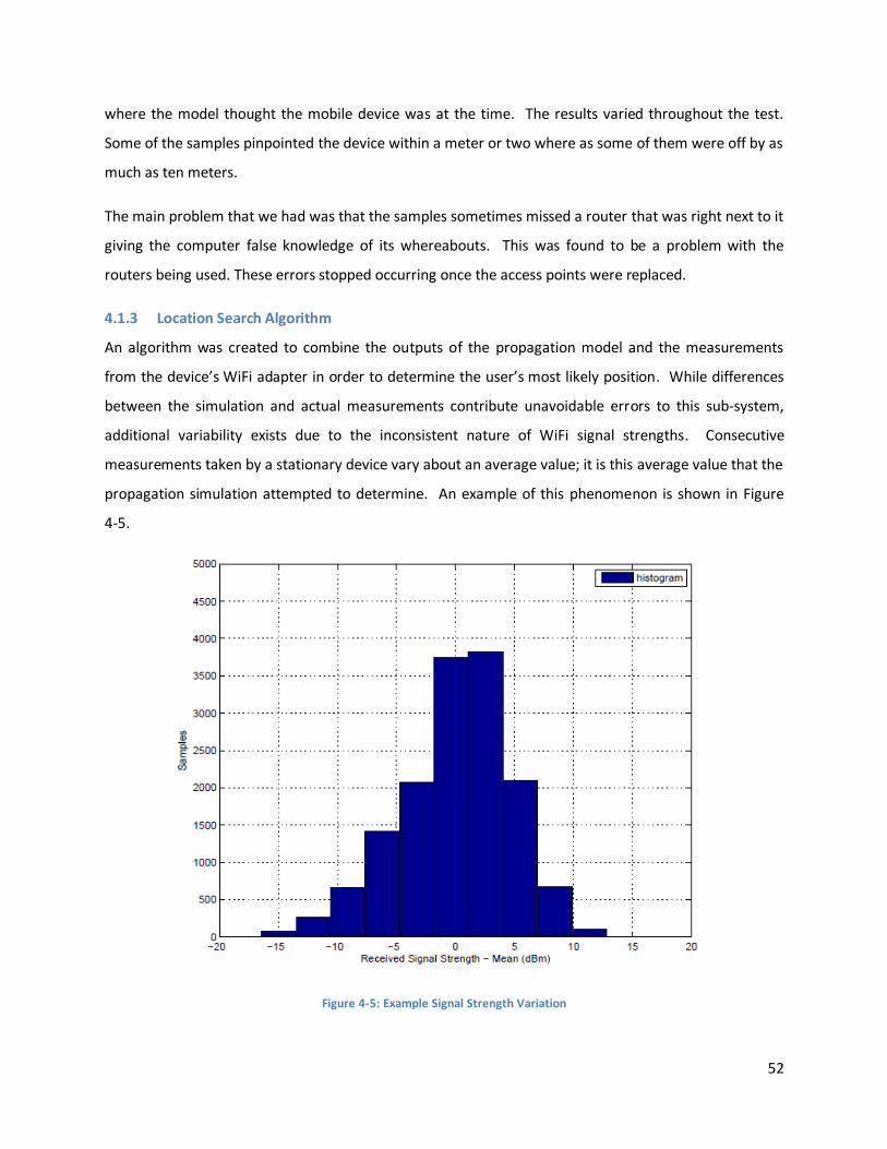
52
where the model thought the mobile device was at the time. The results varied throughout the test.
Some of the samples pinpointed the device within a meter or two where as some of them were off by as
much as ten meters.
The main problem that we had was that the samples sometimes missed a router that was right next to it
giving the computer false knowledge of its whereabouts. This was found to be a problem with the
routers being used. These errors stopped occurring once the access points were replaced.
4.1.3 Location Search Algorithm
An algorithm was created to combine the outputs of the propagation model and the measurements
from the device’s WiFi adapter in order to determine the user’s most likely position. While differences
between the simulation and actual measurements contribute unavoidable errors to this sub-system,
additional variability exists due to the inconsistent nature of WiFi signal strengths. Consecutive
measurements taken by a stationary device vary about an average value; it is this average value that the
propagation simulation attempted to determine. An example of this phenomenon is shown in Figure
4-5.
Figure 4-5: Example Signal Strength Variation
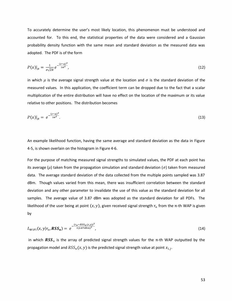
53
To accurately determine the user’s most likely location, this phenomenon must be understood and
accounted for. To this end, the statistical properties of the data were considered and a Gaussian
probability density function with the same mean and standard deviation as the measured data was
adopted. The PDF is of the form
, (12)
in which is the average signal strength value at the location and is the standard deviation of the
measured values. In this application, the coefficient term can be dropped due to the fact that a scalar
multiplication of the entire distribution will have no effect on the location of the maximum or its value
relative to other positions. The distribution becomes
. (13)
An example likelihood function, having the same average and standard deviation as the data in Figure
4-5, is shown overlain on the histogram in Figure 4-6.
For the purpose of matching measured signal strengths to simulated values, the PDF at each point has
its average ( ) taken from the propagation simulation and standard deviation ( ) taken from measured
data. The average standard deviation of the data collected from the multiple points sampled was 3.87
dBm. Though values varied from this mean, there was insufficient correlation between the standard
deviation and any other parameter to invalidate the use of this value as the standard deviation for all
samples. The average value of 3.87 dBm was adopted as the standard deviation for all PDFs. The
likelihood of the user being at point , given received signal strength from the -th WAP is given
by
, (14)
in which is the array of predicted signal strength values for the -th WAP outputted by the
propagation model and is the predicted signal strength value at point .
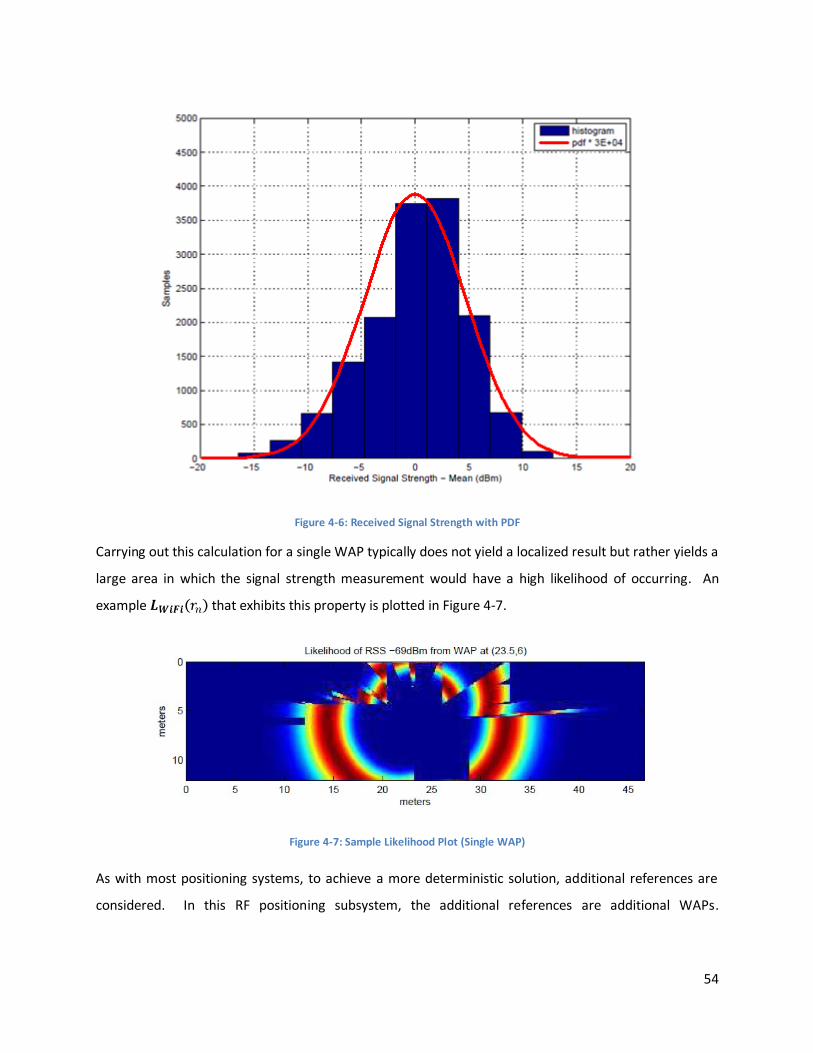
54
Figure 4-6: Received Signal Strength with PDF
Carrying out this calculation for a single WAP typically does not yield a localized result but rather yields a
large area in which the signal strength measurement would have a high likelihood of occurring. An
example that exhibits this property is plotted in Figure 4-7.
Figure 4-7: Sample Likelihood Plot (Single WAP)
As with most positioning systems, to achieve a more deterministic solution, additional references are
considered. In this RF positioning subsystem, the additional references are additional WAPs.
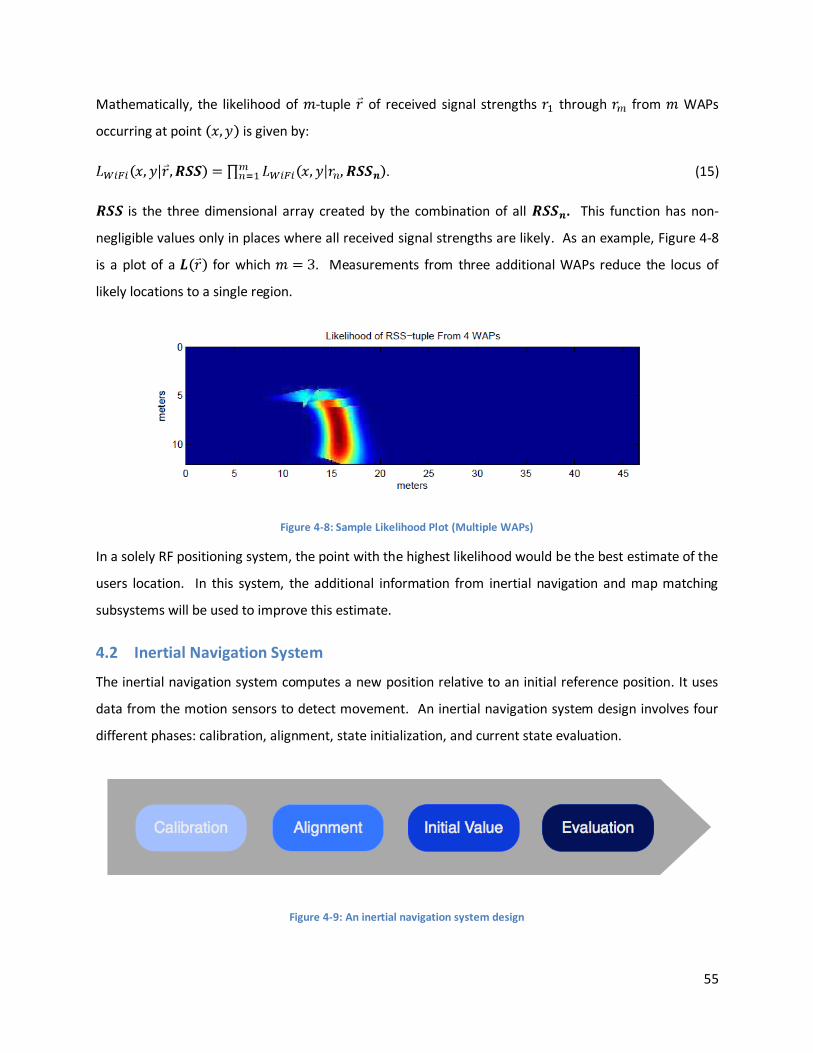
55
Mathematically, the likelihood of -tuple of received signal strengths through from WAPs
occurring at point is given by:
. (15)
is the three dimensional array created by the combination of all . This function has non-
negligible values only in places where all received signal strengths are likely. As an example, Figure 4-8
is a plot of a for which . Measurements from three additional WAPs reduce the locus of
likely locations to a single region.
Figure 4-8: Sample Likelihood Plot (Multiple WAPs)
In a solely RF positioning system, the point with the highest likelihood would be the best estimate of the
users location. In this system, the additional information from inertial navigation and map matching
subsystems will be used to improve this estimate.
4.2 Inertial Navigation System
The inertial navigation system computes a new position relative to an initial reference position. It uses
data from the motion sensors to detect movement. An inertial navigation system design involves four
different phases: calibration, alignment, state initialization, and current state evaluation.
Figure 4-9: An inertial navigation system design

56
1. Calibration: This stage provides coefficients for use in the interpretation of the raw motion
sensor output.
2. Alignment: This stage provides the axis and orientation to interpret the calibrated data in
relation to the Earths coordination.
3. State Initialization: This stage provides the initial position and velocity, which it gets from
another reference positioning method.
4. Current State Evaluation: This stage computes the position relative to the reference position.
4.2.1 Calibration
The HTC Hero sensors, including the accelerometer and the digital compass, need to be calibrated to
correct errors before the data is processed in the alignment phase. The accelerometer chip, built-in to
the HTC Hero, is the Bosch Sensortec’s 3-axis BMA150 and the digital compass is the Asahi Kasei's
AK8973. Before calibrating the sensor data from the phone, we performed several tests to analyze the
accuracy of the sensor.
The testing software module, implemented in java on the Android operating system, takes samples from
the accelerometer and the digital compass at the fastest rate allowed by Android, which is
approximately 10 – 20 milliseconds per sample. The accelerometer measures the acceleration in three
axes in m/s2. The axes output of the accelerometer is relative to the phone’s orientation and will be
referred to as “the device’s coordination system.” The output of the accelerometer is such that when
the device is free falling in a vacuum, the chip will not detect any force exerted on the device, which will
produce zeros for all three outputs.
We calibrated the device’s accelerometer by placing it still on a horizontal plane parallel to the Earth’s
surface. In this case the device is only subjected to the gravity of the Earth, which is approximately
9.807 m/s2 in the z-axis of the device’s coordination system.
When the device is lying flat, the accelerations in three axes of the device should be:
(16)
The g in the formula is the gravity of the Earth. Therefore, we use this assumption to calibrate by setting
a coefficient offset:
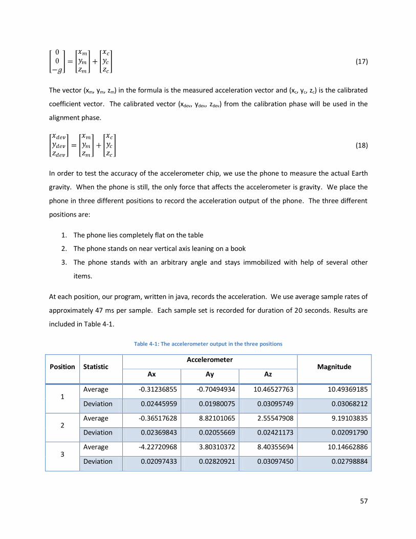
57
(17)
The vector (xm, ym, zm) in the formula is the measured acceleration vector and (xc, yc, zc) is the calibrated
coefficient vector. The calibrated vector (xdev, ydev, zdev) from the calibration phase will be used in the
alignment phase.
(18)
In order to test the accuracy of the accelerometer chip, we use the phone to measure the actual Earth
gravity. When the phone is still, the only force that affects the accelerometer is gravity. We place the
phone in three different positions to record the acceleration output of the phone. The three different
positions are:
1. The phone lies completely flat on the table
2. The phone stands on near vertical axis leaning on a book
3. The phone stands with an arbitrary angle and stays immobilized with help of several other
items.
At each position, our program, written in java, records the acceleration. We use average sample rates of
approximately 47 ms per sample. Each sample set is recorded for duration of 20 seconds. Results are
included in Table 4-1.
Table 4-1: The accelerometer output in the three positions
Position Statistic Accelerometer
Magnitude Ax Ay Az
1 Average -0.31236855 -0.70494934 10.46527763 10.49369185
Deviation 0.02445959 0.01980075 0.03095749 0.03068212
2 Average -0.36517628 8.82101065 2.55547908 9.19103835
Deviation 0.02369843 0.02055669 0.02421173 0.02091790
3 Average -4.22720968 3.80310372 8.40355694 10.14662886
Deviation 0.02097433 0.02820921 0.03097450 0.02798884
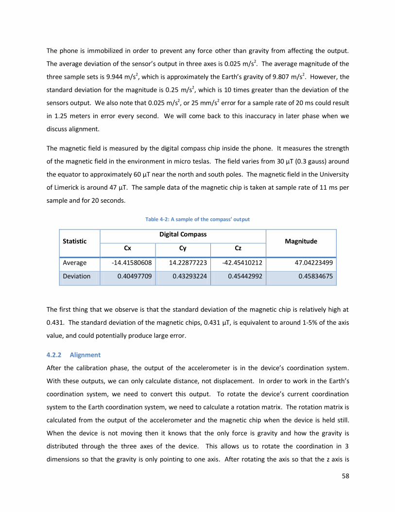
58
The phone is immobilized in order to prevent any force other than gravity from affecting the output.
The average deviation of the sensor’s output in three axes is 0.025 m/s2. The average magnitude of the
three sample sets is 9.944 m/s2, which is approximately the Earth’s gravity of 9.807 m/s2. However, the
standard deviation for the magnitude is 0.25 m/s2, which is 10 times greater than the deviation of the
sensors output. We also note that 0.025 m/s2, or 25 mm/s2 error for a sample rate of 20 ms could result
in 1.25 meters in error every second. We will come back to this inaccuracy in later phase when we
discuss alignment.
The magnetic field is measured by the digital compass chip inside the phone. It measures the strength
of the magnetic field in the environment in micro teslas. The field varies from 30 µT (0.3 gauss) around
the equator to approximately 60 µT near the north and south poles. The magnetic field in the University
of Limerick is around 47 µT. The sample data of the magnetic chip is taken at sample rate of 11 ms per
sample and for 20 seconds.
Table 4-2: A sample of the compass’ output
Statistic Digital Compass
Magnitude Cx Cy Cz
Average -14.41580608 14.22877223 -42.45410212 47.04223499
Deviation 0.40497709 0.43293224 0.45442992 0.45834675
The first thing that we observe is that the standard deviation of the magnetic chip is relatively high at
0.431. The standard deviation of the magnetic chips, 0.431 µT, is equivalent to around 1-5% of the axis
value, and could potentially produce large error.
4.2.2 Alignment
After the calibration phase, the output of the accelerometer is in the device’s coordination system.
With these outputs, we can only calculate distance, not displacement. In order to work in the Earth’s
coordination system, we need to convert this output. To rotate the device’s current coordination
system to the Earth coordination system, we need to calculate a rotation matrix. The rotation matrix is
calculated from the output of the accelerometer and the magnetic chip when the device is held still.
When the device is not moving then it knows that the only force is gravity and how the gravity is
distributed through the three axes of the device. This allows us to rotate the coordination in 3
dimensions so that the gravity is only pointing to one axis. After rotating the axis so that the z axis is

59
pointing to the sky, we then incorporate the magnetic output to calculate rotation in the x and y axes.
This also assumes that only the Earth’s magnetic field is affecting the device, which means that there are
no other magnetic devices such as electrical wires or magnets nearby. If this assumption is true then we
can rotate the current rotation matrix so that y-axis is pointing north and the x-axis is pointing east. This
coordination system is illustrated in Figure 4-10.
Figure 4-10: The Earth’s coordination system in three dimensions
The most important factor that contributes to an accurate rotation matrix is the input gravity from the
accelerometer and the input geomagnetic field from the magnetic chip. The accuracy of the inputs
determines accuracy of the output of our alignment phase. This process is continuous, which means
that the device must compute a new rotation matrix whenever the phone is changing position.
Therefore, whenever the device is rotated, the system needs a new Earth’s gravity measurement and
new Earth’s magnetic field associated with the new position in order to compute a new rotation matrix.
If the device is being held perfectly still, we can easily compute the rotation matrix with high accuracy.
However, when a person is holding the phone, there will be a slight shaking from the hand of the person
which adds acceleration to the output of the accelerometer other than just the Earth’s gravity.
The method we used to detect whether the current acceleration consists of only gravity is by comparing
the magnitude of the total calibrated acceleration at the current moment with the Earth’s gravitational
magnitude, which is 9.807 m/s2. If this magnitude is within our error threshold of ±1 m/s2, the Earth’s
gravity associated with current position is recorded. Besides the error that could result from the sensor
itself, there is another problem that could potentially occur. If the person is moving at a rate such that
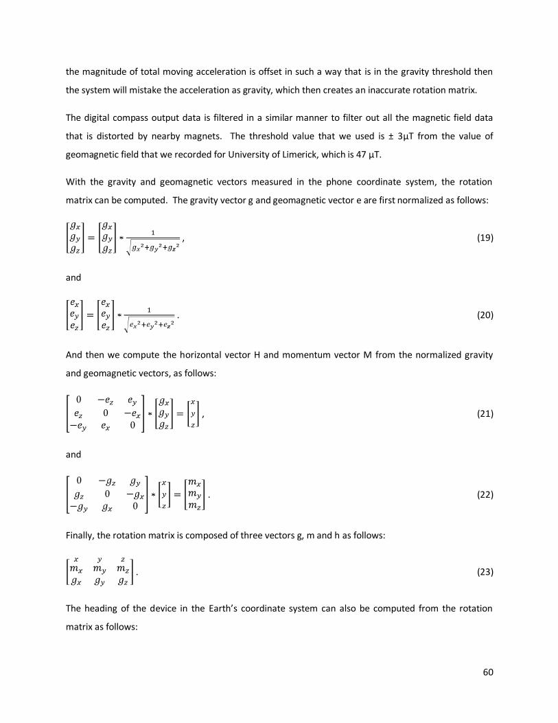
60
the magnitude of total moving acceleration is offset in such a way that is in the gravity threshold then
the system will mistake the acceleration as gravity, which then creates an inaccurate rotation matrix.
The digital compass output data is filtered in a similar manner to filter out all the magnetic field data
that is distorted by nearby magnets. The threshold value that we used is ± 3µT from the value of
geomagnetic field that we recorded for University of Limerick, which is 47 µT.
With the gravity and geomagnetic vectors measured in the phone coordinate system, the rotation
matrix can be computed. The gravity vector g and geomagnetic vector e are first normalized as follows:
, (19)
and
. (20)
And then we compute the horizontal vector H and momentum vector M from the normalized gravity
and geomagnetic vectors, as follows:
, (21)
and
. (22)
Finally, the rotation matrix is composed of three vectors g, m and h as follows:
. (23)
The heading of the device in the Earth’s coordinate system can also be computed from the rotation
matrix as follows:
61
. (24)
4.2.3 Initial Value
The output of the inertial navigation system is the displacement from a reference point. Therefore, an
initial position is needed to make use of this output. The initial position makes a fundamental difference
in accuracy of the whole system from the beginning. Therefore, an accurate initial position is necessary.
This position is provided from the WiFi positioning system.
4.2.4 Evaluation
Knowing the initial value, the next position will be calculated by applying Newton’s second law of
motion. There are three different methods that were tested for determining an accurate displacement:
Integration of acceleration outputs with respect to time to compute the velocity and the
distance moved.
Using acceleration output to detect pedestrian step occurrence and the step length to find the
distance moved.
Using accelerations output to detect current motion status of the user and apply standard
walking velocity to find the distance moved.
The first method of calculating the displacement from the current location is by integrating the
acceleration output over time. Using discrete integration, the velocity is computed by integrating the
acceleration over the time difference every time a sample is recorded. Then, the velocity can be
integrated one more time to compute the displacement. However, this method has been determined to
provide the least accurate displacement among the three methods. The reason is due to hardware
limitation of the HTC Hero. The accelerometer is not accurate enough to provide data with small
enough inaccuracy. Moreover, since the error is then integrated twice to compute the displacement,
the small error can be elevated into a large error in a small amount of time. This integration drift causes
this method to provide poor results, considering the digital compass yields a result with moderate error.
The second method is to detect the step occurrence of the user’s walking from the output of the
accelerometer. However, this method is very hard to apply in our situation where the user is holding
the equipment. Traditional methods of detecting the pedestrian step often use the sensors installed in
the shoes or on the leg where movement can be distinguished clearly. When the user is holding the
phone, the data output does not clearly characterize the person’s stride. Moreover, the data is also

62
subjected to a lot of noise caused by the lagging of a person’s hand while holding the phone. Combined
with a relatively large error from the phone sensors, this method is not suitable for our estimation of the
inertial displacement.
The last method, which is the method we chose to apply, is to detect the whether or not the user is
moving. Using the samples recorded and computing the standard deviation of these samples, we are
able to detect movement due to a larger than normal observed deviation in the acceleration
measurement. Our application collects the last fifty samples and computes the standard deviation of
these samples. Since the fastest sampling rate of the HTC Hero is approximately 20 ms, fifty samples are
about the last second. This provides enough cushions to detect a transition between the stationary
state and the motion state fast enough and prevent the noise from affecting our result.
Figure 4-11: Motion Detection from Inertial Navigation System
The Figure 4-11 is the data collected when the user is holding the phone and starts walking for a short
period before stopping. The blue line is the magnitude of the aligned and calibrated acceleration output
from the accelerometer. The green line is the standard deviation of the last 50 samples. From our
measured test data, the average standard deviation when stationary is approximately 0.1 m/s2 while the
average standard deviation in motion is approximately 1.4 m/s2. Therefore, the standard deviation
threshold is set at 0.7 m/s2.
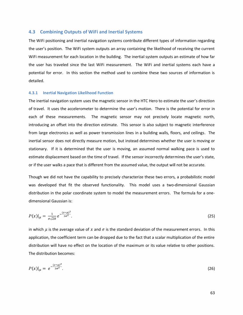
63
4.3 Combining Outputs of WiFi and Inertial Systems
The WiFi positioning and inertial navigation systems contribute different types of information regarding
the user’s position. The WiFi system outputs an array containing the likelihood of receiving the current
WiFi measurement for each location in the building. The inertial system outputs an estimate of how far
the user has traveled since the last WiFi measurement. The WiFi and inertial systems each have a
potential for error. In this section the method used to combine these two sources of information is
detailed.
4.3.1 Inertial Navigation Likelihood Function
The inertial navigation system uses the magnetic sensor in the HTC Hero to estimate the user’s direction
of travel. It uses the accelerometer to determine the user’s motion. There is the potential for error in
each of these measurements. The magnetic sensor may not precisely locate magnetic north,
introducing an offset into the direction estimate. This sensor is also subject to magnetic interference
from large electronics as well as power transmission lines in a building walls, floors, and ceilings. The
inertial sensor does not directly measure motion, but instead determines whether the user is moving or
stationary. If it is determined that the user is moving, an assumed normal walking pace is used to
estimate displacement based on the time of travel. If the sensor incorrectly determines the user’s state,
or if the user walks a pace that is different from the assumed value, the output will not be accurate.
Though we did not have the capability to precisely characterize these two errors, a probabilistic model
was developed that fit the observed functionality. This model uses a two-dimensional Gaussian
distribution in the polar coordinate system to model the measurement errors. The formula for a one-
dimensional Gaussian is:
. (25)
in which is the average value of and is the standard deviation of the measurement errors. In this
application, the coefficient term can be dropped due to the fact that a scalar multiplication of the entire
distribution will have no effect on the location of the maximum or its value relative to other positions.
The distribution becomes:
. (26)
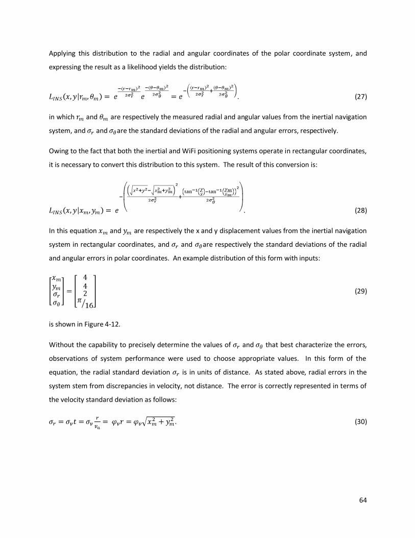
64
Applying this distribution to the radial and angular coordinates of the polar coordinate system, and
expressing the result as a likelihood yields the distribution:
. (27)
in which and are respectively the measured radial and angular values from the inertial navigation
system, and and are the standard deviations of the radial and angular errors, respectively.
Owing to the fact that both the inertial and WiFi positioning systems operate in rectangular coordinates,
it is necessary to convert this distribution to this system. The result of this conversion is:
. (28)
In this equation and are respectively the x and y displacement values from the inertial navigation
system in rectangular coordinates, and and are respectively the standard deviations of the radial
and angular errors in polar coordinates. An example distribution of this form with inputs:
(29)
is shown in Figure 4-12.
Without the capability to precisely determine the values of and that best characterize the errors,
observations of system performance were used to choose appropriate values. In this form of the
equation, the radial standard deviation is in units of distance. As stated above, radial errors in the
system stem from discrepancies in velocity, not distance. The error is correctly represented in terms of
the velocity standard deviation as follows:
. (30)
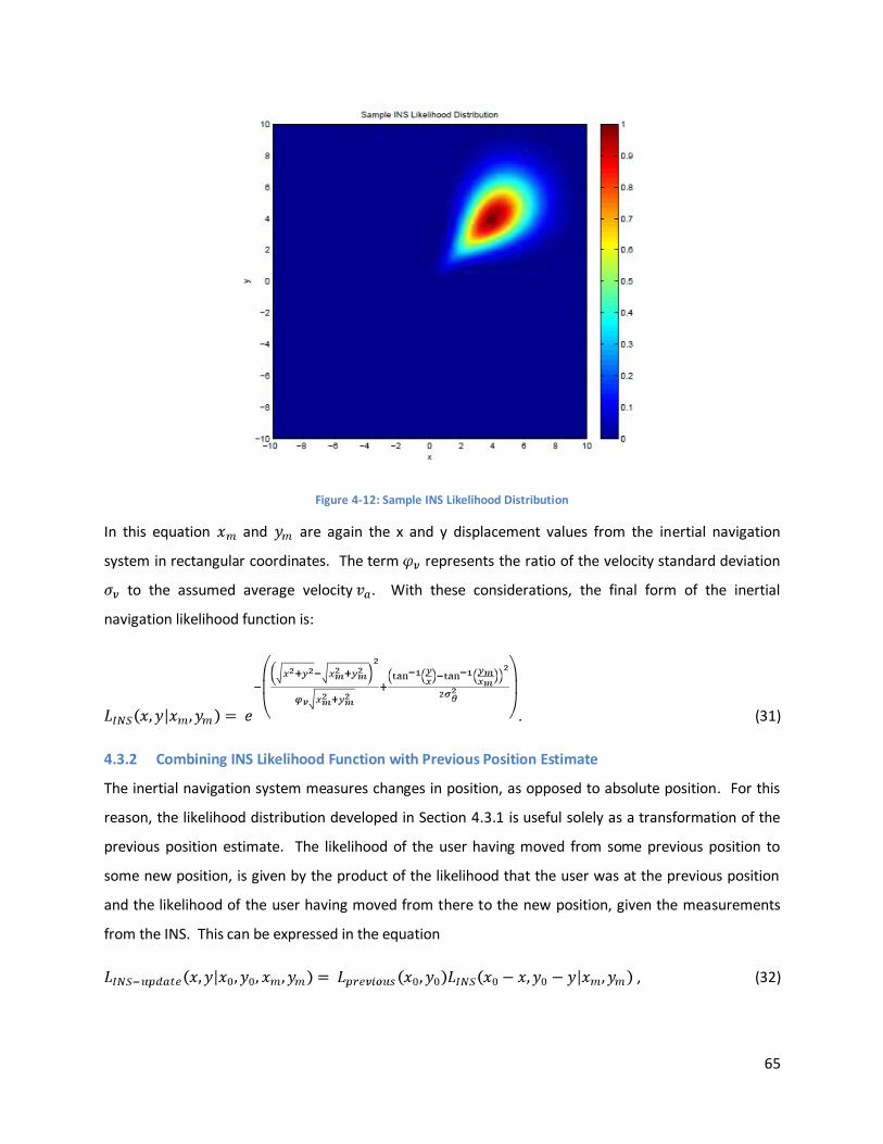
65
Figure 4-12: Sample INS Likelihood Distribution
In this equation and are again the x and y displacement values from the inertial navigation
system in rectangular coordinates. The term represents the ratio of the velocity standard deviation
to the assumed average velocity . With these considerations, the final form of the inertial
navigation likelihood function is:
. (31)
4.3.2 Combining INS Likelihood Function with Previous Position Estimate
The inertial navigation system measures changes in position, as opposed to absolute position. For this
reason, the likelihood distribution developed in Section 4.3.1 is useful solely as a transformation of the
previous position estimate. The likelihood of the user having moved from some previous position to
some new position, is given by the product of the likelihood that the user was at the previous position
and the likelihood of the user having moved from there to the new position, given the measurements
from the INS. This can be expressed in the equation
, (32)
66
In which terms and define the previous position and terms and define displacement
measured by the INS. It follows that the likelihood of the user being at a location is the sum the
preceding equation for all previous positions. This is expressed in the equation
, (33)
In which the terms and define displacement measured by the INS. This method, while correct, is
not computationally efficient. Due to the fact that the INS likelihood function has negligible values at
large distances from the measured location, the region of the summation is limited to those points of
the previous likelihood distribution near the new point. The equation
, (34)
limits the integrals to values lying in a ten meter square, centered about the new point.
4.3.3 Combining INS-updated Position and WiFi Position Estimate
In order to determine the most likely location of the user, the likelihood array resulting from the
combination of the INS likelihood function and the previous likelihood estimate must be combined with
the likelihood function from the WiFi positioning systems location search algorithm. The combination,
in which each element of the INS array is multiplied by the corresponding element of the WiFi likelihood
array, is expressed as follows:
. (35)
The maximum value of the likelihood array is the system’s current estimate of the user’s
position. This array is stored in memory for use as in the next cycle of calculations.
4.4 Summary
This positioning system uses multiple sources of information to determine its location. Measurements
of WiFi signal strengths from multiple access points are compared to data generated by a propagation
model to estimate the user’s location in the building. The point at which the received signal strengths
are most likely to have occurred is chosen. Data from inertial and magnetic sensors is used to estimate
the user’s change in position between WiFi samples. These two estimates area combined with
information from previous sample periods to determine the user’s most likely location. An example of
the HTC Hero determining the user’s location is displayed in Figure 4-13.
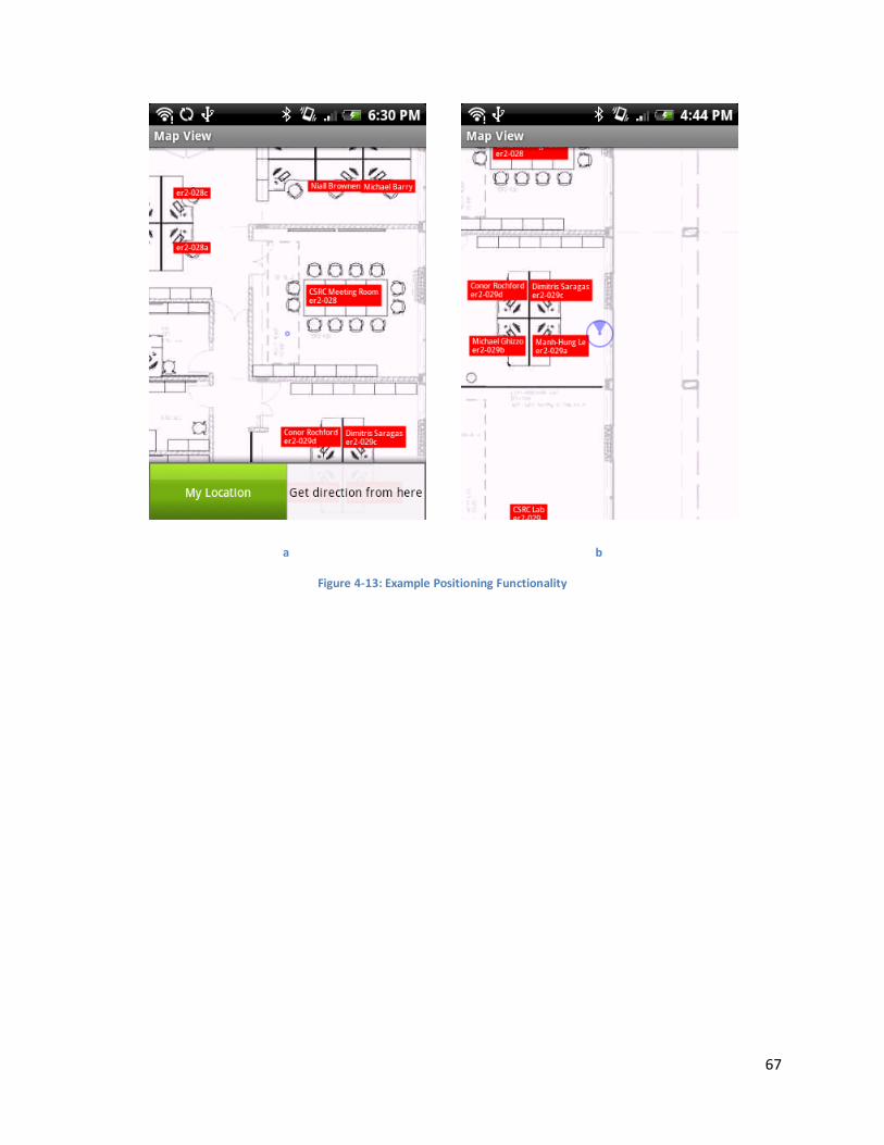
67
a b
Figure 4-13: Example Positioning Functionality
68
5 Navigation
The navigation system is responsible for determining an optimal route to a destination. It consists of
graphing functionality and a routing algorithm.
5.1 Graphing
With the current position of the user known, it is important to determine the destination that the user
wants to go to. The output of this module is a path that guides the user to their desired destination. In
order to achieve this task, we choose to represent the map of the building in a graph on which the
routing algorithm can operate.
A graph can be a complex system of nodes and links that are connected in a tree-like data structure. A
node represents a specific position in a building and tells the information about that position. A building
map often consists of four different elements: rooms, hallways, stairs/elevators, and large rooms. All of
these elements will be represented by nodes with coordinates and information associated with them.
The room node is used to represent a small area enclosed area. The large room node is used to
represent any open space larger than a room. The reason that we distinguish between these two types
of rooms is because we will choose to represent a small room with a single node while a large room will
contain many nodes. This has to do with the accuracy of the positioning methods and the propagation
of WiFi degrading much less in free space. The stair and elevator nodes are type of node which connects
two floors inside of a building. Its special characteristic is that two nodes representing stairs on two
different floors will have a same coordinate, thus the cost of travelling between them cannot be
determined by the Euclidean distance but rather be assigned by a special weighting scheme. The last
element is a hallway, which is typically the most common type of node in a building. It represents
intersection and traffic direction. It serves as the media to connect all the other elements in the system.
A link is a line on which a user can traverse the distance between two nodes. The user can move from a
node to a different node only when there is a link between them. The link is associated with a cost that
represents the distance to travel through the link. The distance between two nodes can be known by
computing the Euclidean distance between their coordinates. In some special cases such as the link
connecting two stairs node or two elevators node, its cost is assigned a special weight.
Our graph is constructed manually in such a way that satisfies our two characteristics: all hallway links
must be either horizontal or vertical lines and there are no links connecting two points that have a wall
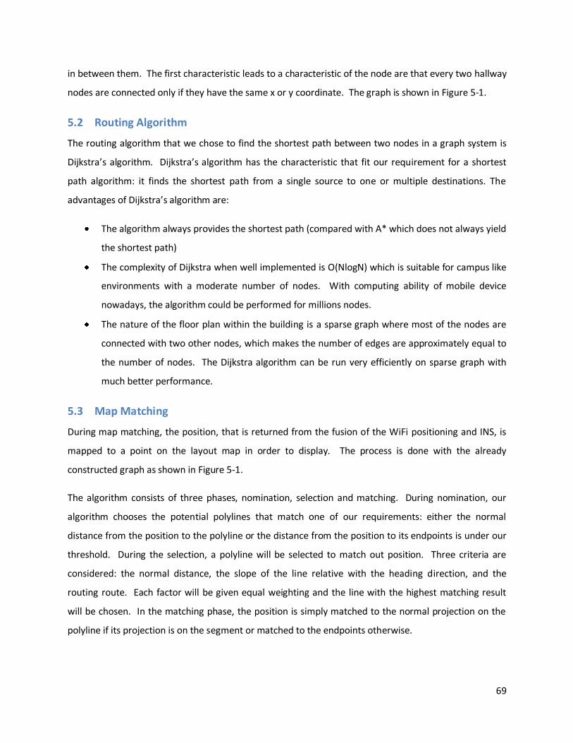
69
in between them. The first characteristic leads to a characteristic of the node are that every two hallway
nodes are connected only if they have the same x or y coordinate. The graph is shown in Figure 5-1.
5.2 Routing Algorithm
The routing algorithm that we chose to find the shortest path between two nodes in a graph system is
Dijkstra’s algorithm. Dijkstra’s algorithm has the characteristic that fit our requirement for a shortest
path algorithm: it finds the shortest path from a single source to one or multiple destinations. The
advantages of Dijkstra’s algorithm are:
The algorithm always provides the shortest path (compared with A* which does not always yield
the shortest path)
The complexity of Dijkstra when well implemented is O(NlogN) which is suitable for campus like
environments with a moderate number of nodes. With computing ability of mobile device
nowadays, the algorithm could be performed for millions nodes.
The nature of the floor plan within the building is a sparse graph where most of the nodes are
connected with two other nodes, which makes the number of edges are approximately equal to
the number of nodes. The Dijkstra algorithm can be run very efficiently on sparse graph with
much better performance.
5.3 Map Matching
During map matching, the position, that is returned from the fusion of the WiFi positioning and INS, is
mapped to a point on the layout map in order to display. The process is done with the already
constructed graph as shown in Figure 5-1.
The algorithm consists of three phases, nomination, selection and matching. During nomination, our
algorithm chooses the potential polylines that match one of our requirements: either the normal
distance from the position to the polyline or the distance from the position to its endpoints is under our
threshold. During the selection, a polyline will be selected to match out position. Three criteria are
considered: the normal distance, the slope of the line relative with the heading direction, and the
routing route. Each factor will be given equal weighting and the line with the highest matching result
will be chosen. In the matching phase, the position is simply matched to the normal projection on the
polyline if its projection is on the segment or matched to the endpoints otherwise.
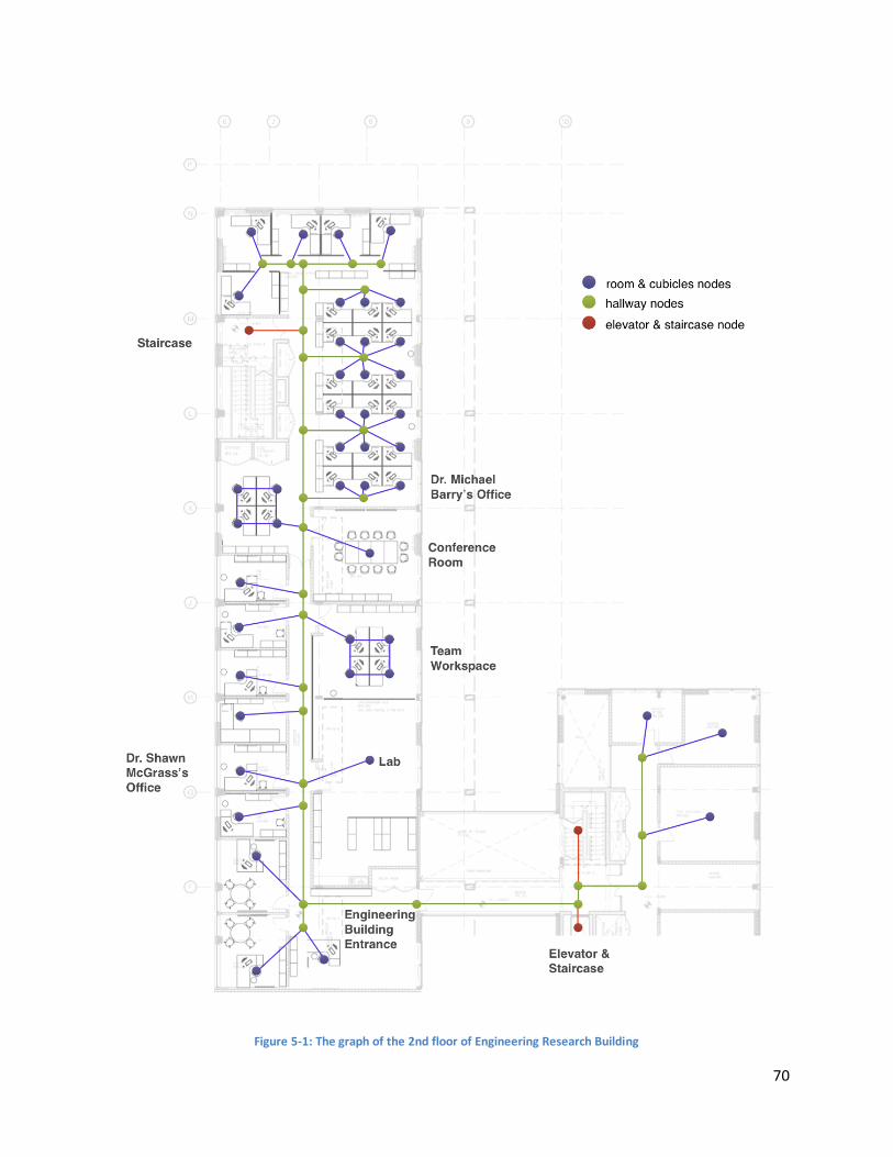
70
Figure 5-1: The graph of the 2nd floor of Engineering Research Building
71
Figure 5-2: Map Matching Algorithm example
Figure 5-2 illustrates an example of our matching algorithm. The blue arrow represents the path that
the user should walk through in order to get to the destination. The grey point is the previous point that
was matched on the route. The blue point is the current position returned from the positioning system
that needs to be matched using our algorithm. The blue fan that attached to the blue point is the
heading from the compass. The yellow is the actual position of the user on the route. Using our criteria
to nominate polylines, the red lines are included because the distance from the blue point to their
endpoint is within our threshold. The green line also is nominated because it is within the threshold
normal distance to the blue point. The grey line is considered because it is the line which the previous
matched position, the grey point, is on. The purple line is considered because it is in our routing path to
the destination. Coming to the selection phase, if we only considered normal distance, the red line will
be chosen with its minimal distance to the blue position. However, given the current route displayed by
the blue arrow and the heading direction, the purple line will be chosen by our algorithm. Our blue
position will mapped to the projection point on the purple line, which is illustrated by the purple dotted
line.
5.4 Summary
The navigation subsystem operates on a graph that represents locations and routes in the building.
Locations are represented as a type of node in the graph. Nodes are designated as a room, a hallway, or
a staircase. Dijkstra’s routing algorithm is chosen as a suitable method for finding the optimal route from
a location to a destination in this graph. It is suitable because it is computationally efficient and it is
guaranteed to find the optimal route. S map-matching system is used to correctly map a user’s location
in space to a node or link in the building graph prior to routing algorithm computation.
72
6 Prototype Implementation
This project consists of a number of subsystems. The following chapter describes the implementation of
these subsystems as a Java application.
6.1 Android Platform Architecture
The software application of our project is implemented on the Google Android phone the HTC Hero.
The HTC Hero is running the Google Android Operating System. The operating system is a Java virtual
machine called Dalvik running on a Linux Kernel. The architecture of the operating system includes four
layers of software as shown in the Figure 2-18. More information can be found on Android official
developer website.
Our application will be implemented using the Application Framework modules and access to the Linux
Kernel through provided Application Programming Interfaces (APIs) in the operating system libraries.
The application is written in Java and its system files will be managed by the Dalvik Virtual Machine.
Our application thread is running under the framework activity and is called at the beginning of the
software launch. The Activity is a thread responsible for processing information and communicating
inside the software. It also manages View framework responsible for graphical representation of
information to be displayed to user. The view is running its own thread to be refreshed periodically to
display the information.
6.2 Software System Design
Our applications can be viewed as four major blocks of processing: positioning, navigation, database,
and interface. Each block is responsible to different functionality of the application. Positioning block is
responsible for finding the current location of the user by combining WiFi positioning and inertial
navigation system. Navigation block is responsible for performing routing algorithm to find the shortest
route between two positions and map matching algorithm to correlate the position on the map for
graphical representation. Database block is responsible for searching information of people and
building. Interface block is responsible for the graphical representation of the information and
interaction with user. The Figure 6-1 shows the software functional blocks and its main components.
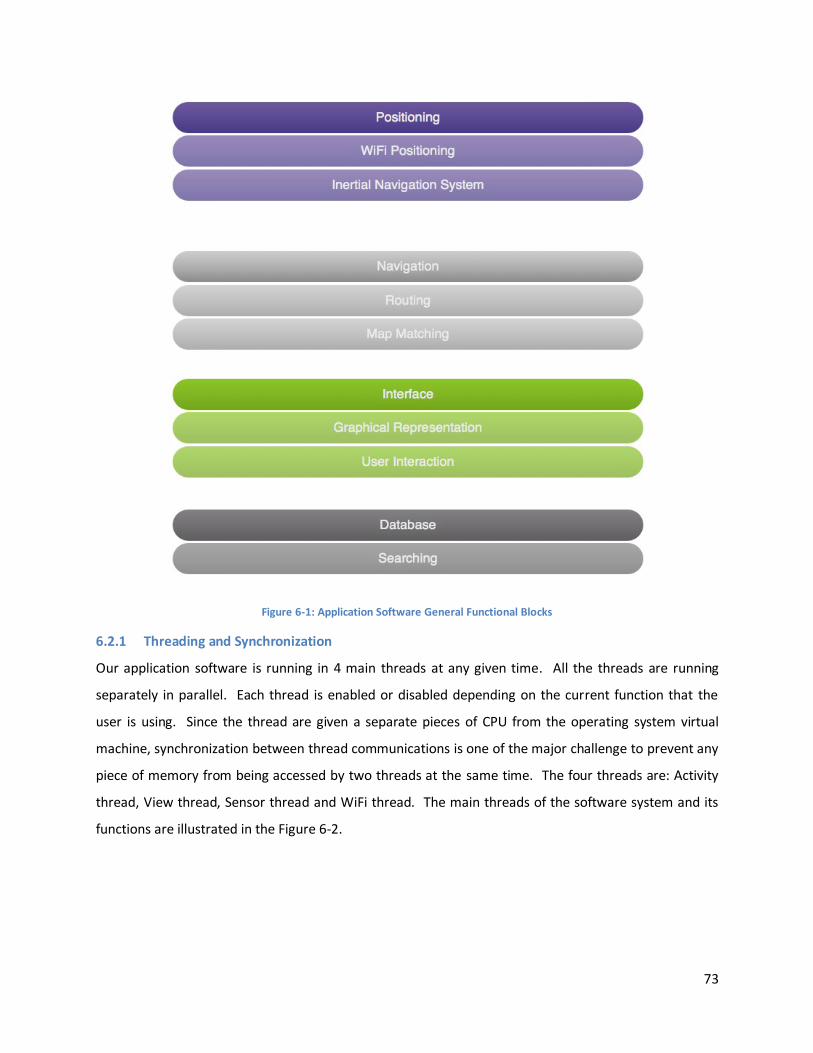
73
Figure 6-1: Application Software General Functional Blocks
6.2.1 Threading and Synchronization
Our application software is running in 4 main threads at any given time. All the threads are running
separately in parallel. Each thread is enabled or disabled depending on the current function that the
user is using. Since the thread are given a separate pieces of CPU from the operating system virtual
machine, synchronization between thread communications is one of the major challenge to prevent any
piece of memory from being accessed by two threads at the same time. The four threads are: Activity
thread, View thread, Sensor thread and WiFi thread. The main threads of the software system and its
functions are illustrated in the Figure 6-2.
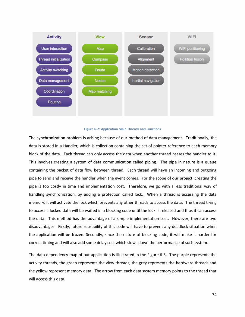
74
Figure 6-2: Application Main Threads and Functions
The synchronization problem is arising because of our method of data management. Traditionally, the
data is stored in a Handler, which is collection containing the set of pointer reference to each memory
block of the data. Each thread can only access the data when another thread passes the handler to it.
This involves creating a system of data communication called piping. The pipe in nature is a queue
containing the packet of data flow between thread. Each thread will have an incoming and outgoing
pipe to send and receive the handler when the event comes. For the scope of our project, creating the
pipe is too costly in time and implementation cost. Therefore, we go with a less traditional way of
handling synchronization, by adding a protection called lock. When a thread is accessing the data
memory, it will activate the lock which prevents any other threads to access the data. The thread trying
to access a locked data will be waited in a blocking code until the lock is released and thus it can access
the data. This method has the advantage of a simple implementation cost. However, there are two
disadvantages. Firstly, future reusability of this code will have to prevent any deadlock situation when
the application will be frozen. Secondly, since the nature of blocking code, it will make it harder for
correct timing and will also add some delay cost which slows down the performance of such system.
The data dependency map of our application is illustrated in the Figure 6-3. The purple represents the
activity threads, the green represents the view threads, the grey represents the hardware threads and
the yellow represent memory data. The arrow from each data system memory points to the thread that
will access this data.
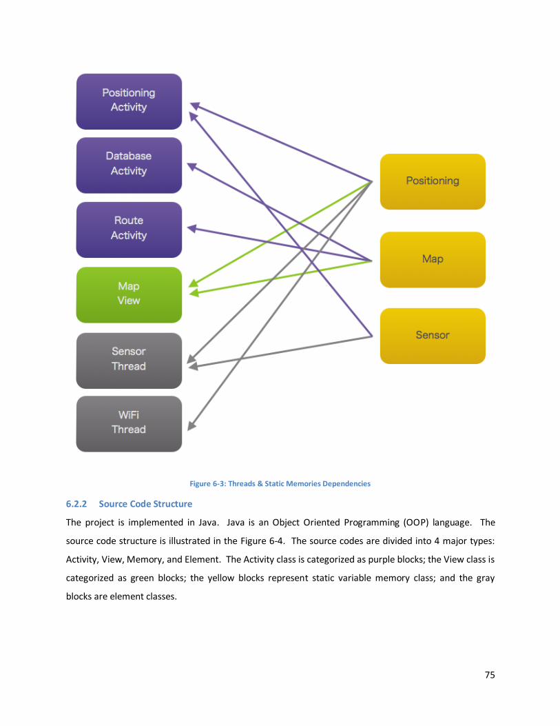
75
Figure 6-3: Threads & Static Memories Dependencies
6.2.2 Source Code Structure
The project is implemented in Java. Java is an Object Oriented Programming (OOP) language. The
source code structure is illustrated in the Figure 6-4. The source codes are divided into 4 major types:
Activity, View, Memory, and Element. The Activity class is categorized as purple blocks; the View class is
categorized as green blocks; the yellow blocks represent static variable memory class; and the gray
blocks are element classes.
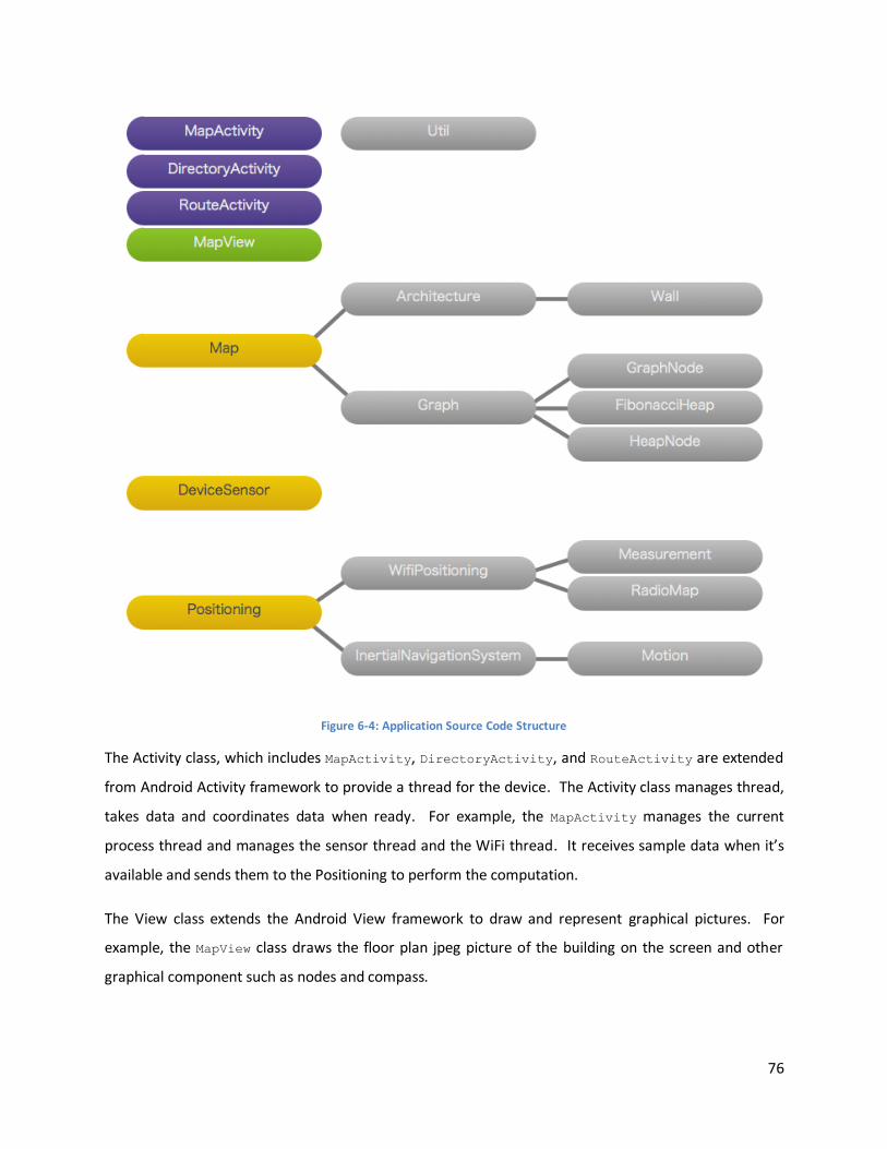
76
Figure 6-4: Application Source Code Structure
The Activity class, which includes MapActivity, DirectoryActivity, and RouteActivity are extended
from Android Activity framework to provide a thread for the device. The Activity class manages thread,
takes data and coordinates data when ready. For example, the MapActivity manages the current
process thread and manages the sensor thread and the WiFi thread. It receives sample data when it’s
available and sends them to the Positioning to perform the computation.
The View class extends the Android View framework to draw and represent graphical pictures. For
example, the MapView class draws the floor plan jpeg picture of the building on the screen and other
graphical component such as nodes and compass.
77
The Memory class is implemented as static memory block which makes it available across all the threads
in the application without passing the handler. It uses lock and synchronized feature to implements
synchronization.
The Element classes are fundamental blocks which contain functional methods for algorithm and
represent different type of data. For example, the Graph class contains the list of GraphNode nodes and
can perform routing algorithm.
6.3 Functional Blocks
The following sections describe the implementation of each functional block inside the application.
6.3.1 Inertial Navigation System
The Inertial Navigation System (INS), is implemented under the MapActivity class, the class initializes
the thread for receiving samples from the accelerometer and digital compass when available. The
hardware sensors are called from the application through Android Application Programming Interface
(API). The API will start when receiving command from the user to search for the current location. After
that, the samples are received periodically at the sampling rate specified and triggered the sensor
thread. After processing the data, the sensor thread then stores it in memory class DeviceSensor. The
sensor thread performs calibration upon receiving the sample if the sample is from the accelerometer.
Then the data is filtered to get the gravity or geomagnetic values. These two values are then combined
to get the rotation matrix and get the orientation values including the current heading of the phone.
The accelerometer values will be push at the end of a queue. We used a queue data structure to store
the last hundred samples. Upon receiving new values, the queue will remove the value at the top of the
queue, which is the oldest value in the queue and replace it with the new value at the end of the queue.
The standard deviation is computed for the entire sensor samples set in the queue. The current status
of the device is stationary when the standard deviation is below the threshold and in motion if it is
above the threshold.
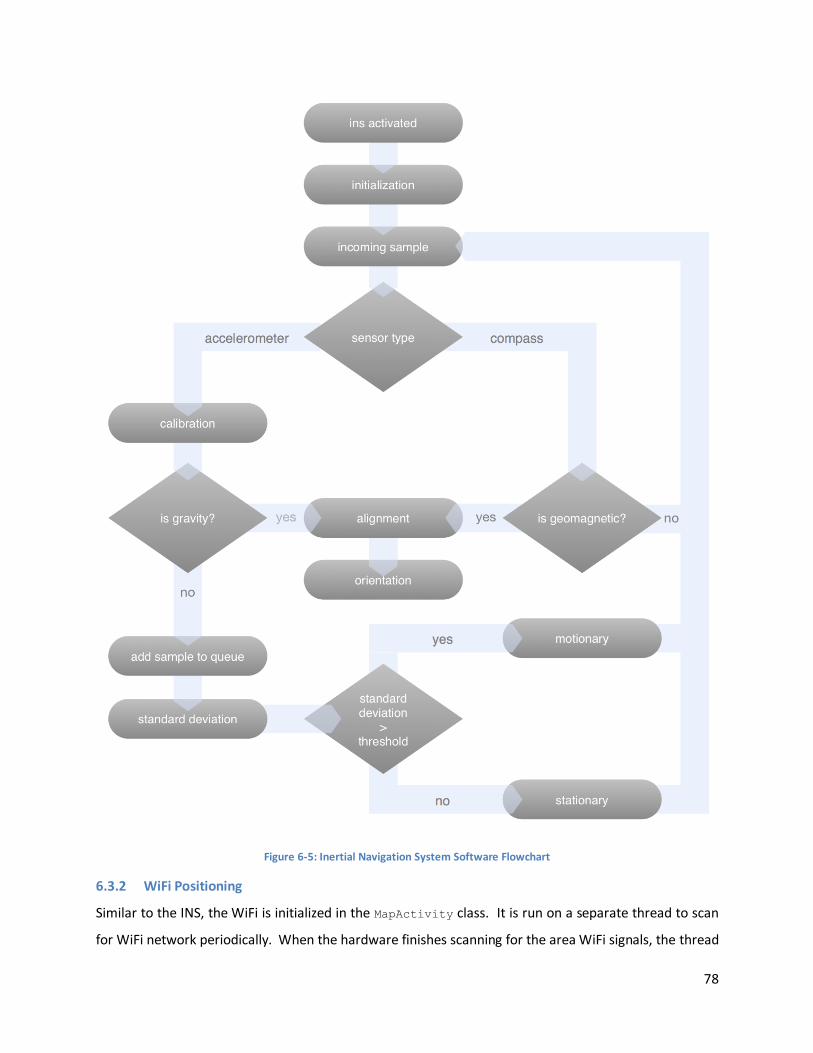
78
Figure 6-5: Inertial Navigation System Software Flowchart
6.3.2 WiFi Positioning
Similar to the INS, the WiFi is initialized in the MapActivity class. It is run on a separate thread to scan
for WiFi network periodically. When the hardware finishes scanning for the area WiFi signals, the thread
79
will receive the sample measurement. After receiving the measurements, the thread filters only signals
that are known in the simulated database by comparing their unique Basic Service Set Identifier (BSSID).
This set of signal measurements will be used to correlate with the simulated propagation. The
correlation computational performance is O(area/resolution2) with the resolution is number of discrete
values in a meter from the propagation simulated model.
6.3.3 Positioning Fusion
After the WiFi correlation is ready, the WiFi thread will start fusing the correlation model with the INS
movement vector. An array of size twice a constant we define as “effective radius” which is the radius
of the discrete Gaussian probability distribution. The computational performance of computing the
Gaussian is O(rgaussian2). Then this Gaussian distribution array will be shifted on the last values of the
probability density function (PDF) map to compute the new PDF. The computational load is
O(area/resolution2 * rgaussian2). Since the computation is a floating point multiplication, we see that the
effective size plays an important role in the computational load. A 10 meters Gaussian radius in the
distribution array can result in 3 million floating point multiplication every second.
6.3.4 Database
Although the HTC Hero has the capability of creating a database using SQL in the Content Provider
module of Android Operating System, we don’t use this database in our application. The SQL would
have provided us with better synchronization and portability with a web interface and sharing system.
However, with the timeframe of the project, we decided to implement only a pseudo database using
text file to store directory information and our application will construct the database inside the
program by parsing those text files. The text files that are used to construct our database are: nodes.txt,
edges.txt, and wall.txt. Each of them contains information about the graph nodes inside the building,
the edges that connects them and the physical walls respectively. The nodes information includes the
geographic coordination in the building, the type of the nodes, the identifier of the room and the name
of the person which it belongs to. The edges information contains on which nodes are connected to
each other in a form of an adjacent list. The wall information includes their coordinates in the building.
The text files can be found in Appendix C: Database files.
6.3.5 Routing
The Dijsktra algorithm implementation is in Graph class. The Graph class also contains the list of nodes
which can be accessed by the routing algorithm. The input of the routing algorithm is the id of source
node and the id of the destination node. The output of the algorithm is the cost of the shortest path
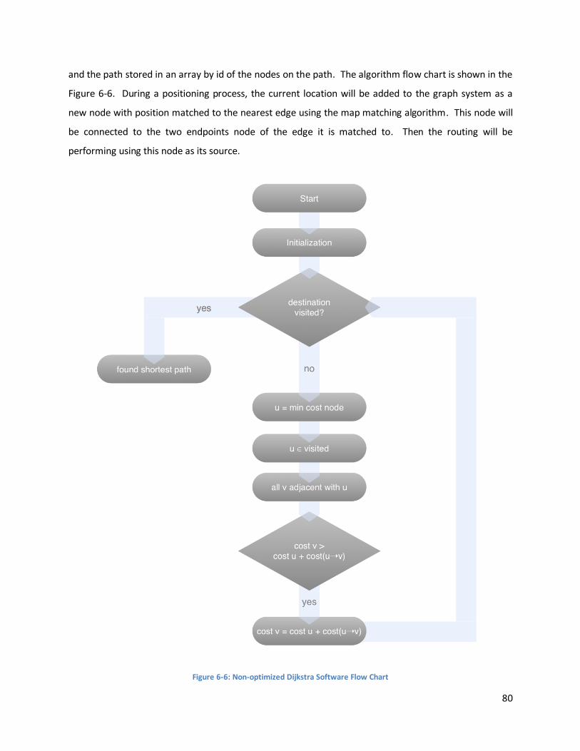
80
and the path stored in an array by id of the nodes on the path. The algorithm flow chart is shown in the
Figure 6-6. During a positioning process, the current location will be added to the graph system as a
new node with position matched to the nearest edge using the map matching algorithm. This node will
be connected to the two endpoints node of the edge it is matched to. Then the routing will be
performing using this node as its source.
Figure 6-6: Non-optimized Dijkstra Software Flow Chart
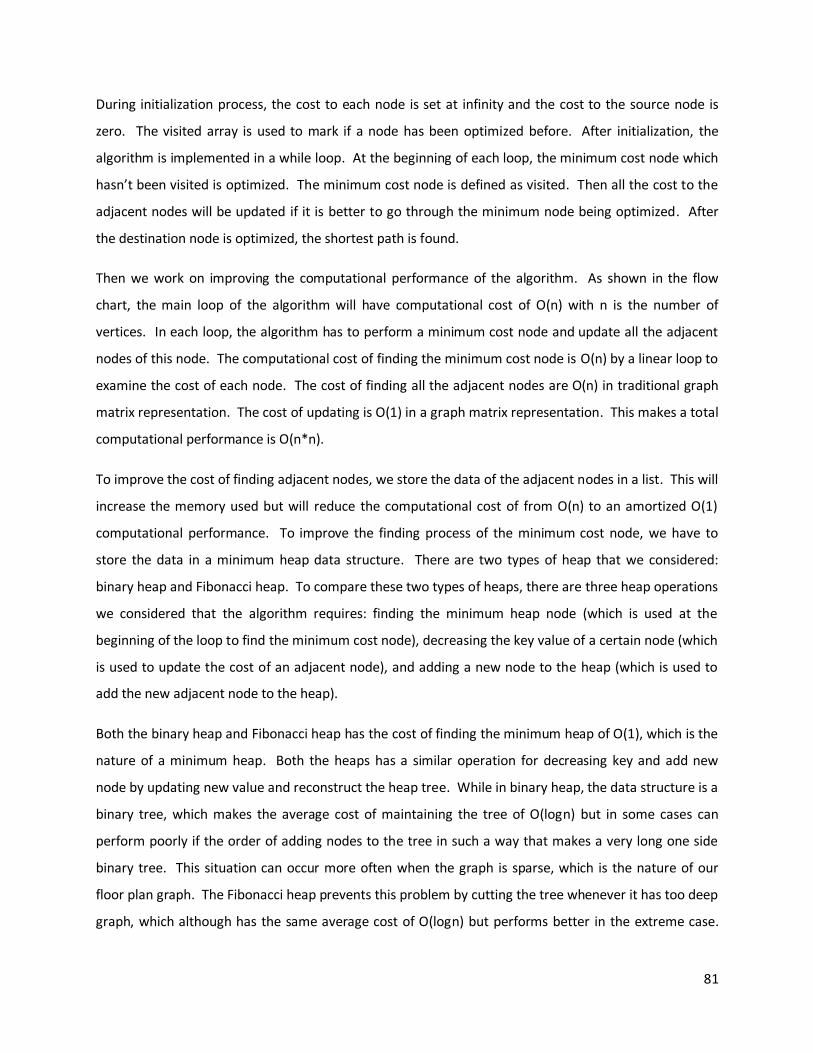
81
During initialization process, the cost to each node is set at infinity and the cost to the source node is
zero. The visited array is used to mark if a node has been optimized before. After initialization, the
algorithm is implemented in a while loop. At the beginning of each loop, the minimum cost node which
hasn’t been visited is optimized. The minimum cost node is defined as visited. Then all the cost to the
adjacent nodes will be updated if it is better to go through the minimum node being optimized. After
the destination node is optimized, the shortest path is found.
Then we work on improving the computational performance of the algorithm. As shown in the flow
chart, the main loop of the algorithm will have computational cost of O(n) with n is the number of
vertices. In each loop, the algorithm has to perform a minimum cost node and update all the adjacent
nodes of this node. The computational cost of finding the minimum cost node is O(n) by a linear loop to
examine the cost of each node. The cost of finding all the adjacent nodes are O(n) in traditional graph
matrix representation. The cost of updating is O(1) in a graph matrix representation. This makes a total
computational performance is O(n*n).
To improve the cost of finding adjacent nodes, we store the data of the adjacent nodes in a list. This will
increase the memory used but will reduce the computational cost of from O(n) to an amortized O(1)
computational performance. To improve the finding process of the minimum cost node, we have to
store the data in a minimum heap data structure. There are two types of heap that we considered:
binary heap and Fibonacci heap. To compare these two types of heaps, there are three heap operations
we considered that the algorithm requires: finding the minimum heap node (which is used at the
beginning of the loop to find the minimum cost node), decreasing the key value of a certain node (which
is used to update the cost of an adjacent node), and adding a new node to the heap (which is used to
add the new adjacent node to the heap).
Both the binary heap and Fibonacci heap has the cost of finding the minimum heap of O(1), which is the
nature of a minimum heap. Both the heaps has a similar operation for decreasing key and add new
node by updating new value and reconstruct the heap tree. While in binary heap, the data structure is a
binary tree, which makes the average cost of maintaining the tree of O(logn) but in some cases can
perform poorly if the order of adding nodes to the tree in such a way that makes a very long one side
binary tree. This situation can occur more often when the graph is sparse, which is the nature of our
floor plan graph. The Fibonacci heap prevents this problem by cutting the tree whenever it has too deep
graph, which although has the same average cost of O(logn) but performs better in the extreme case.
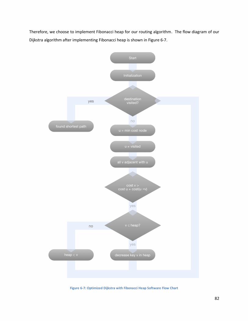
82
Therefore, we choose to implement Fibonacci heap for our routing algorithm. The flow diagram of our
Dijkstra algorithm after implementing Fibonacci heap is shown in Figure 6-7.
Figure 6-7: Optimized Dijkstra with Fibonacci Heap Software Flow Chart
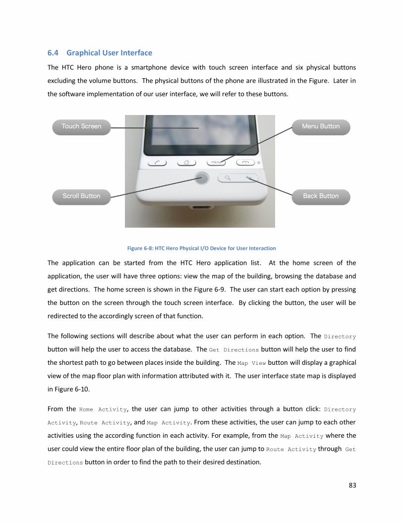
83
6.4 Graphical User Interface
The HTC Hero phone is a smartphone device with touch screen interface and six physical buttons
excluding the volume buttons. The physical buttons of the phone are illustrated in the Figure. Later in
the software implementation of our user interface, we will refer to these buttons.
Figure 6-8: HTC Hero Physical I/O Device for User Interaction
The application can be started from the HTC Hero application list. At the home screen of the
application, the user will have three options: view the map of the building, browsing the database and
get directions. The home screen is shown in the Figure 6-9. The user can start each option by pressing
the button on the screen through the touch screen interface. By clicking the button, the user will be
redirected to the accordingly screen of that function.
The following sections will describe about what the user can perform in each option. The Directory
button will help the user to access the database. The Get Directions button will help the user to find
the shortest path to go between places inside the building. The Map View button will display a graphical
view of the map floor plan with information attributed with it. The user interface state map is displayed
in Figure 6-10.
From the Home Activity, the user can jump to other activities through a button click: Directory
Activity, Route Activity, and Map Activity. From these activities, the user can jump to each other
activities using the according function in each activity. For example, from the Map Activity where the
user could view the entire floor plan of the building, the user can jump to Route Activity through Get
Directions button in order to find the path to their desired destination.
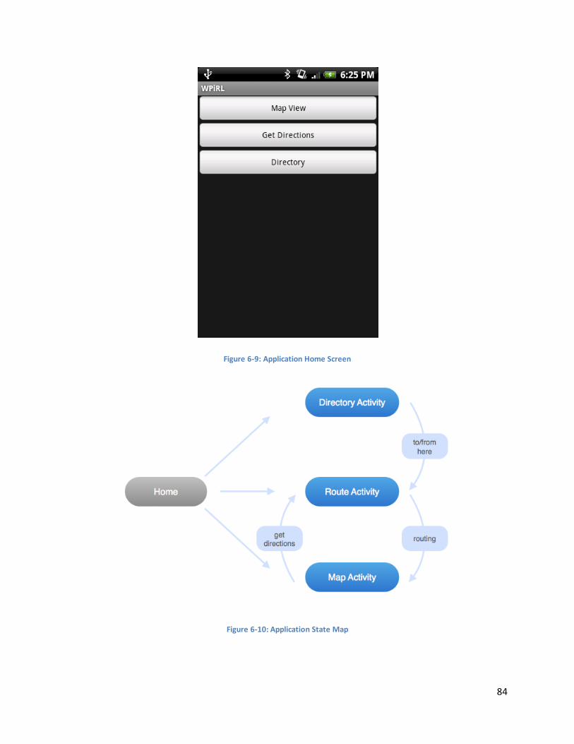
84
Figure 6-9: Application Home Screen
Figure 6-10: Application State Map
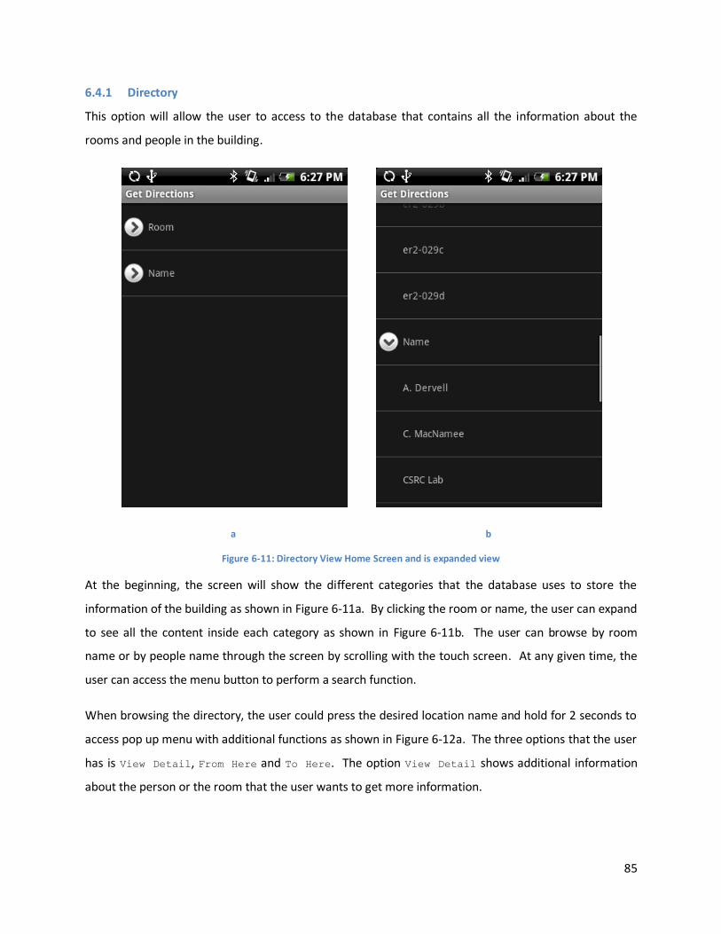
85
6.4.1 Directory
This option will allow the user to access to the database that contains all the information about the
rooms and people in the building.
a b
Figure 6-11: Directory View Home Screen and is expanded view
At the beginning, the screen will show the different categories that the database uses to store the
information of the building as shown in Figure 6-11a. By clicking the room or name, the user can expand
to see all the content inside each category as shown in Figure 6-11b. The user can browse by room
name or by people name through the screen by scrolling with the touch screen. At any given time, the
user can access the menu button to perform a search function.
When browsing the directory, the user could press the desired location name and hold for 2 seconds to
access pop up menu with additional functions as shown in Figure 6-12a. The three options that the user
has is View Detail, From Here and To Here. The option View Detail shows additional information
about the person or the room that the user wants to get more information.
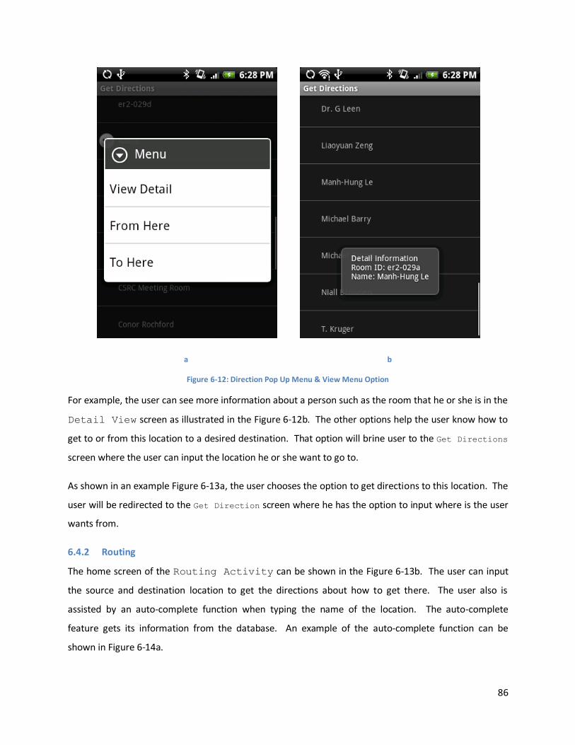
86
a b
Figure 6-12: Direction Pop Up Menu & View Menu Option
For example, the user can see more information about a person such as the room that he or she is in the
Detail View screen as illustrated in the Figure 6-12b. The other options help the user know how to
get to or from this location to a desired destination. That option will brine user to the Get Directions
screen where the user can input the location he or she want to go to.
As shown in an example Figure 6-13a, the user chooses the option to get directions to this location. The
user will be redirected to the Get Direction screen where he has the option to input where is the user
wants from.
6.4.2 Routing
The home screen of the Routing Activity can be shown in the Figure 6-13b. The user can input
the source and destination location to get the directions about how to get there. The user also is
assisted by an auto-complete function when typing the name of the location. The auto-complete
feature gets its information from the database. An example of the auto-complete function can be
shown in Figure 6-14a.

87
a b
Figure 6-13: Linking from the Directory screen to Get Direction screen
a b
Figure 6-14: Auto-complete feature in Routing GUI
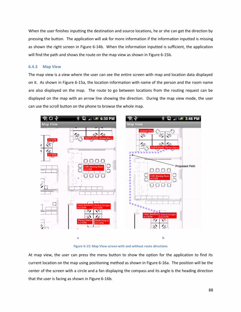
88
When the user finishes inputting the destination and source locations, he or she can get the direction by
pressing the button. The application will ask for more information if the information inputted is missing
as shown the right screen in Figure 6-14b. When the information inputted is sufficient, the application
will find the path and shows the route on the map view as shown in Figure 6-15b.
6.4.3 Map View
The map view is a view where the user can see the entire screen with map and location data displayed
on it. As shown in Figure 6-15a, the location information with name of the person and the room name
are also displayed on the map. The route to go between locations from the routing request can be
displayed on the map with an arrow line showing the direction. During the map view mode, the user
can use the scroll button on the phone to browse the whole map.
a b
Figure 6-15: Map View screen with and without route directions
At map view, the user can press the menu button to show the option for the application to find its
current location on the map using positioning method as shown in Figure 6-16a. The position will be the
center of the screen with a circle and a fan displaying the compass and its angle is the heading direction
that the user is facing as shown in Figure 6-16b.

89
a b
Figure 6-16: Finding the current position of the user and display it on the screen
6.5 Summary
The application is implemented completely in Java and run in the Google Android operating system of
the HTC Hero. The application is a multi threaded object oriented programming project. The INS, WiFi
positioning and positioning integration algorithms are all implemented as a discrete probability
distribution using two dimensional data structure. The positioning integration uses most of the
computational capability of the device. The routing algorithm Dijkstra is implemented using Fibonacci
Heap and achieves optimal result contributing little to the computational load. The application can help
the user to determine the current location and find direction from there to the desired destination. The
user also can browse the directory, view the map and search for a customed route between any
locations inside the building.
90
7 Testing and Results
In order to verify the systems and functionalities described in chapters 4, 0, and 6 a number of tests
were carried out. The procedures and results of these tests are described in this chapter.
7.1 Inertial Navigation System Testing
The purpose of the INS testing was to confirm the functionality described in Section 4.2 and the
probabilistic model of the expected output described in Section 4.3.1.
7.1.1 Quantitative Inertial Navigation System Testing
The accelerometer on the HTC Hero is used to determine whether the user is moving or stationary. The
following test was carried out to assess how accurately the user’s displacement is measured if the
system has determined that the user is moving.
The test was carried out on measured five-meter stretches of hallway in two places on the second floor
of the engineering research building. The two locations are shown in Figure 7-1. To prevent unknowing
contamination of the results cause by bad compass data in any single orientation, data was collected for
both directions of travel on each of two perpendicular stretches of hallway. Trials were conducted in
both locations by two members of the team. Additionally, two motion profiles were used in the
collection of data. In the first, referred to as the “standing” case, the tester started recording data
before beginning to move and stopped recording data after stopping their motion at the end of the
measured path. In the second, referred to as the “walking” case, the tester walked continuously down
the hall way, starting and stopping the recording as the start and finish lines, respectively, were crossed.
Multiple trials were carried out for each combination of test location, direction of motion, tester, and
motion profile.
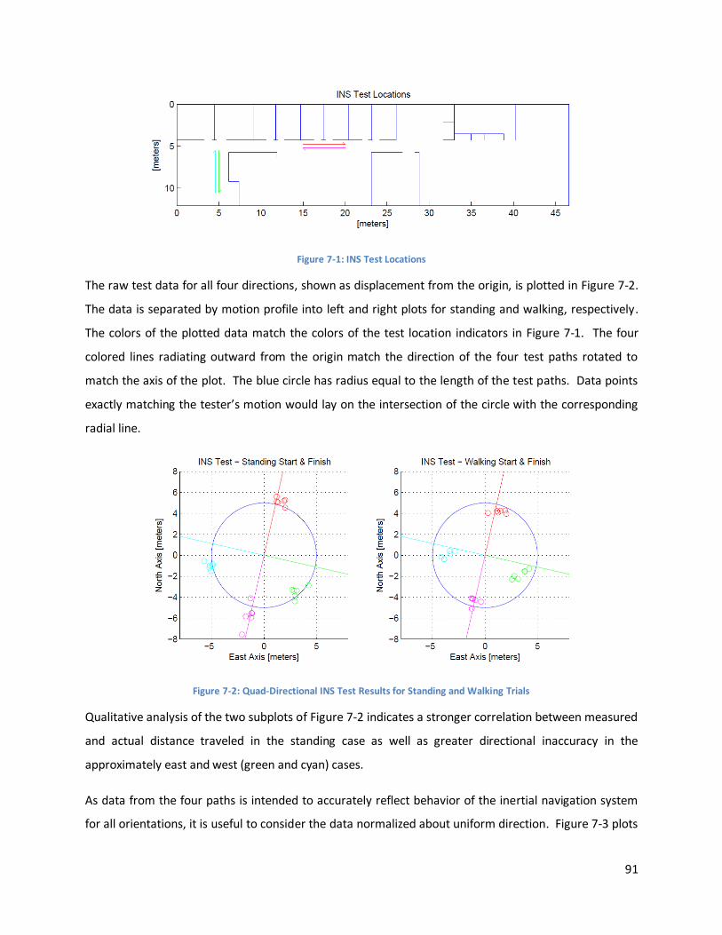
91
Figure 7-1: INS Test Locations
The raw test data for all four directions, shown as displacement from the origin, is plotted in Figure 7-2.
The data is separated by motion profile into left and right plots for standing and walking, respectively.
The colors of the plotted data match the colors of the test location indicators in Figure 7-1. The four
colored lines radiating outward from the origin match the direction of the four test paths rotated to
match the axis of the plot. The blue circle has radius equal to the length of the test paths. Data points
exactly matching the tester’s motion would lay on the intersection of the circle with the corresponding
radial line.
Figure 7-2: Quad-Directional INS Test Results for Standing and Walking Trials
Qualitative analysis of the two subplots of Figure 7-2 indicates a stronger correlation between measured
and actual distance traveled in the standing case as well as greater directional inaccuracy in the
approximately east and west (green and cyan) cases.
As data from the four paths is intended to accurately reflect behavior of the inertial navigation system
for all orientations, it is useful to consider the data normalized about uniform direction. Figure 7-3 plots
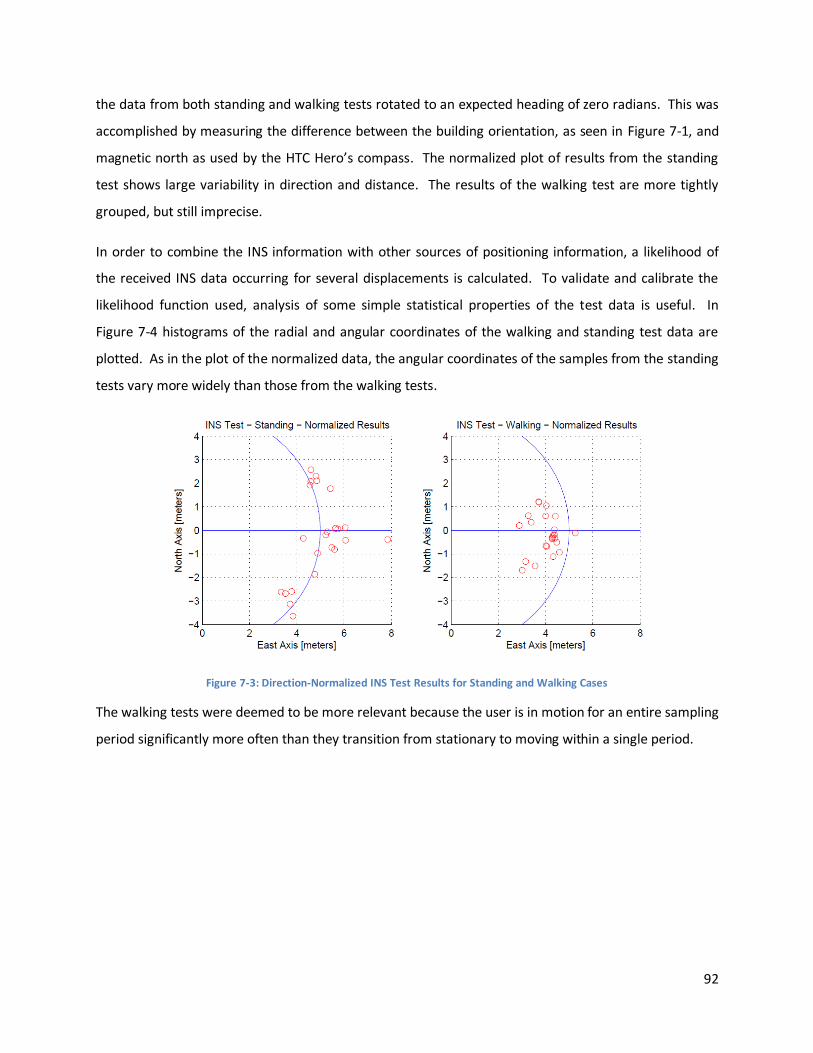
92
the data from both standing and walking tests rotated to an expected heading of zero radians. This was
accomplished by measuring the difference between the building orientation, as seen in Figure 7-1, and
magnetic north as used by the HTC Hero’s compass. The normalized plot of results from the standing
test shows large variability in direction and distance. The results of the walking test are more tightly
grouped, but still imprecise.
In order to combine the INS information with other sources of positioning information, a likelihood of
the received INS data occurring for several displacements is calculated. To validate and calibrate the
likelihood function used, analysis of some simple statistical properties of the test data is useful. In
Figure 7-4 histograms of the radial and angular coordinates of the walking and standing test data are
plotted. As in the plot of the normalized data, the angular coordinates of the samples from the standing
tests vary more widely than those from the walking tests.
Figure 7-3: Direction-Normalized INS Test Results for Standing and Walking Cases
The walking tests were deemed to be more relevant because the user is in motion for an entire sampling
period significantly more often than they transition from stationary to moving within a single period.
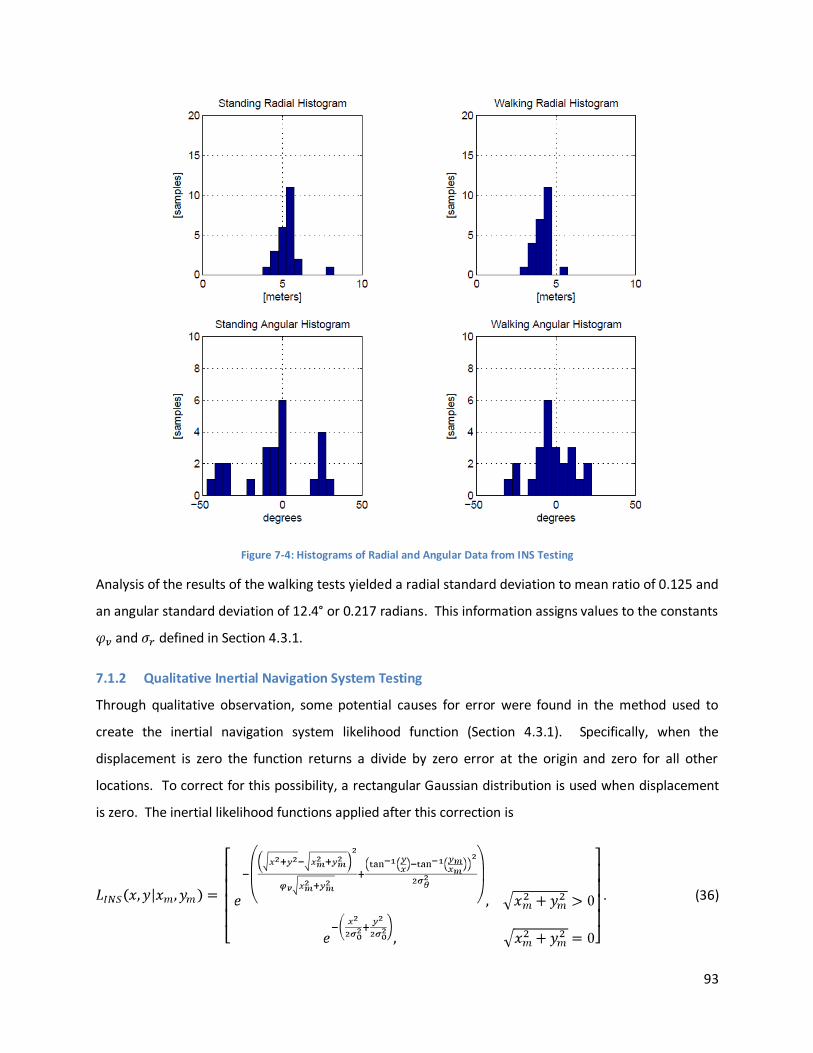
93
Figure 7-4: Histograms of Radial and Angular Data from INS Testing
Analysis of the results of the walking tests yielded a radial standard deviation to mean ratio of 0.125 and
an angular standard deviation of 12.4° or 0.217 radians. This information assigns values to the constants
and defined in Section 4.3.1.
7.1.2 Qualitative Inertial Navigation System Testing
Through qualitative observation, some potential causes for error were found in the method used to
create the inertial navigation system likelihood function (Section 4.3.1). Specifically, when the
displacement is zero the function returns a divide by zero error at the origin and zero for all other
locations. To correct for this possibility, a rectangular Gaussian distribution is used when displacement
is zero. The inertial likelihood functions applied after this correction is
. (36)
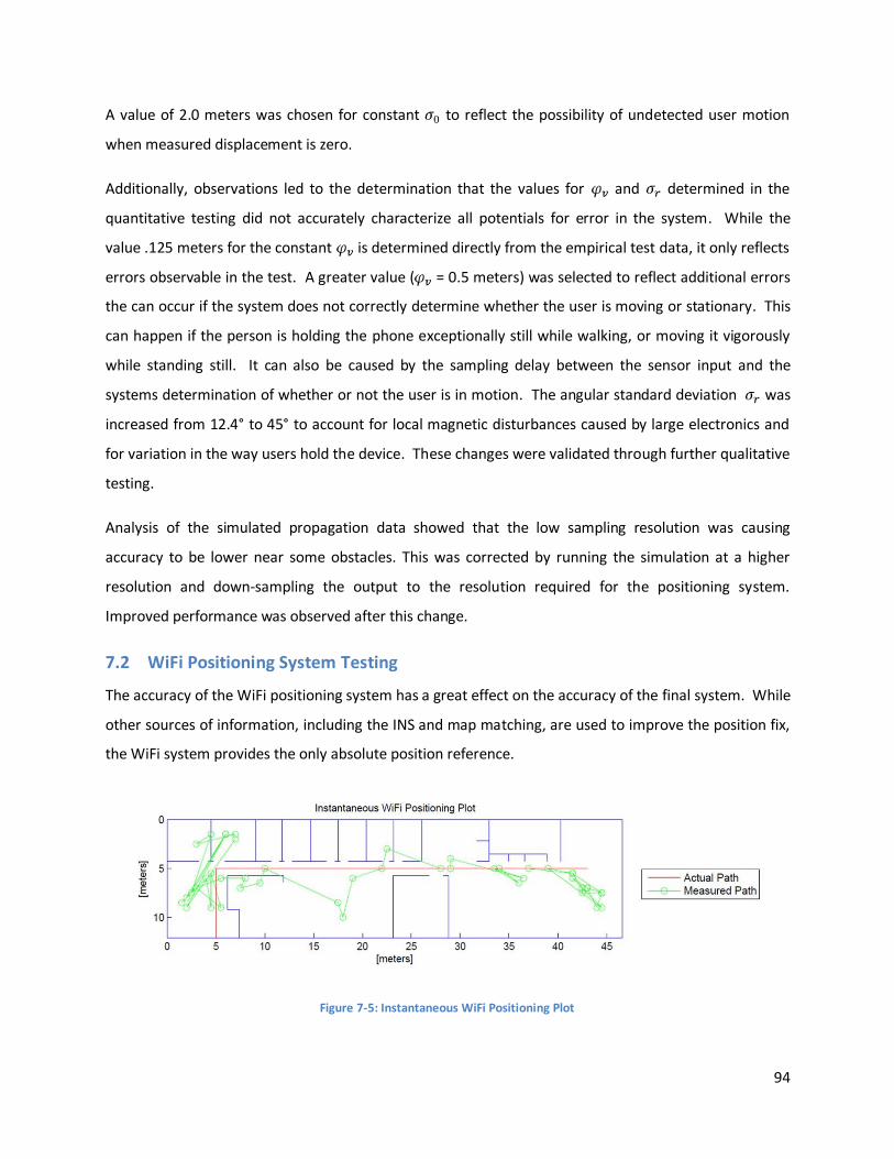
94
A value of 2.0 meters was chosen for constant to reflect the possibility of undetected user motion
when measured displacement is zero.
Additionally, observations led to the determination that the values for and determined in the
quantitative testing did not accurately characterize all potentials for error in the system. While the
value .125 meters for the constant is determined directly from the empirical test data, it only reflects
errors observable in the test. A greater value ( = 0.5 meters) was selected to reflect additional errors
the can occur if the system does not correctly determine whether the user is moving or stationary. This
can happen if the person is holding the phone exceptionally still while walking, or moving it vigorously
while standing still. It can also be caused by the sampling delay between the sensor input and the
systems determination of whether or not the user is in motion. The angular standard deviation was
increased from 12.4° to 45° to account for local magnetic disturbances caused by large electronics and
for variation in the way users hold the device. These changes were validated through further qualitative
testing.
Analysis of the simulated propagation data showed that the low sampling resolution was causing
accuracy to be lower near some obstacles. This was corrected by running the simulation at a higher
resolution and down-sampling the output to the resolution required for the positioning system.
Improved performance was observed after this change.
7.2 WiFi Positioning System Testing
The accuracy of the WiFi positioning system has a great effect on the accuracy of the final system. While
other sources of information, including the INS and map matching, are used to improve the position fix,
the WiFi system provides the only absolute position reference.
Figure 7-5: Instantaneous WiFi Positioning Plot
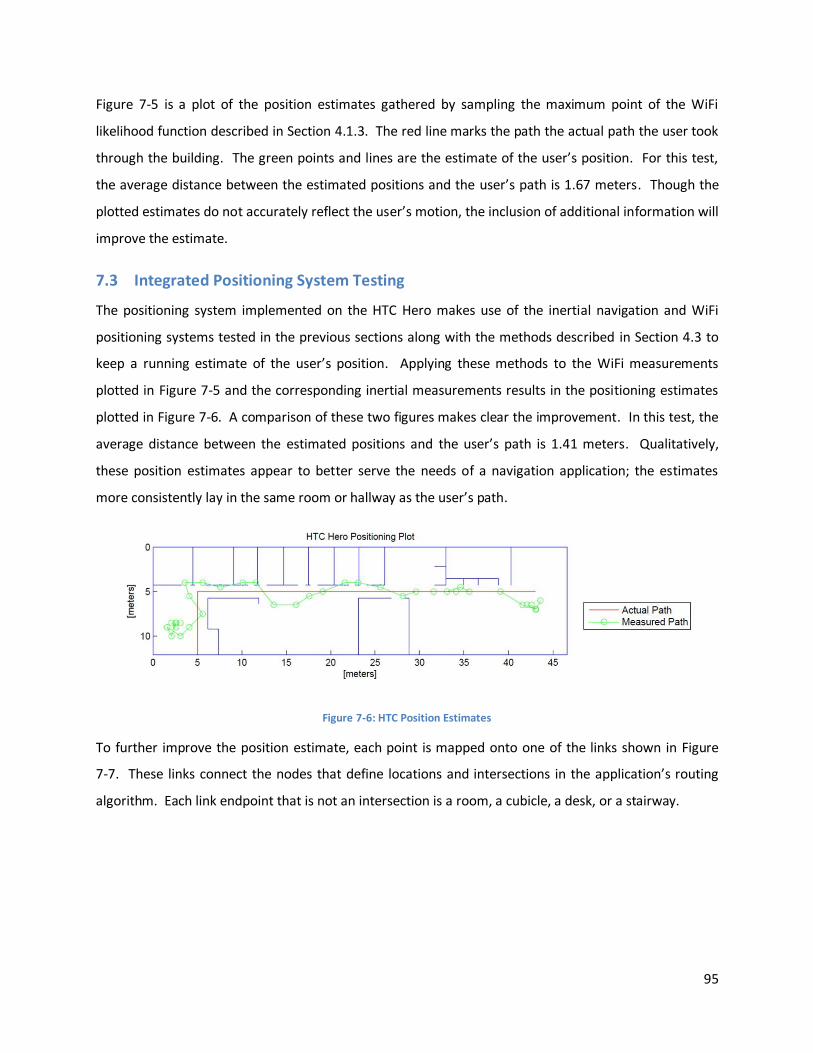
95
Figure 7-5 is a plot of the position estimates gathered by sampling the maximum point of the WiFi
likelihood function described in Section 4.1.3. The red line marks the path the actual path the user took
through the building. The green points and lines are the estimate of the user’s position. For this test,
the average distance between the estimated positions and the user’s path is 1.67 meters. Though the
plotted estimates do not accurately reflect the user’s motion, the inclusion of additional information will
improve the estimate.
7.3 Integrated Positioning System Testing
The positioning system implemented on the HTC Hero makes use of the inertial navigation and WiFi
positioning systems tested in the previous sections along with the methods described in Section 4.3 to
keep a running estimate of the user’s position. Applying these methods to the WiFi measurements
plotted in Figure 7-5 and the corresponding inertial measurements results in the positioning estimates
plotted in Figure 7-6. A comparison of these two figures makes clear the improvement. In this test, the
average distance between the estimated positions and the user’s path is 1.41 meters. Qualitatively,
these position estimates appear to better serve the needs of a navigation application; the estimates
more consistently lay in the same room or hallway as the user’s path.
Figure 7-6: HTC Position Estimates
To further improve the position estimate, each point is mapped onto one of the links shown in Figure
7-7. These links connect the nodes that define locations and intersections in the application’s routing
algorithm. Each link endpoint that is not an intersection is a room, a cubicle, a desk, or a stairway.
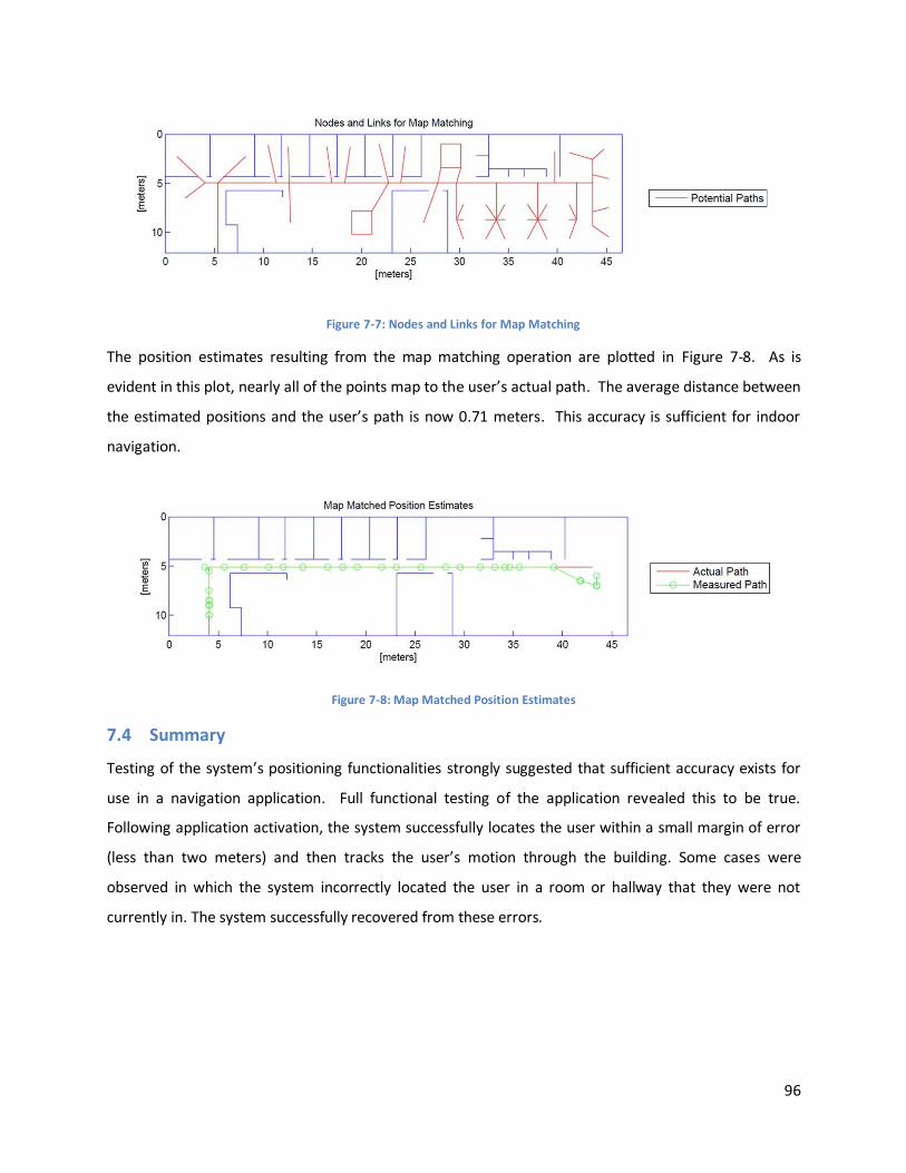
96
Figure 7-7: Nodes and Links for Map Matching
The position estimates resulting from the map matching operation are plotted in Figure 7-8. As is
evident in this plot, nearly all of the points map to the user’s actual path. The average distance between
the estimated positions and the user’s path is now 0.71 meters. This accuracy is sufficient for indoor
navigation.
Figure 7-8: Map Matched Position Estimates
7.4 Summary
Testing of the system’s positioning functionalities strongly suggested that sufficient accuracy exists for
use in a navigation application. Full functional testing of the application revealed this to be true.
Following application activation, the system successfully locates the user within a small margin of error
(less than two meters) and then tracks the user’s motion through the building. Some cases were
observed in which the system incorrectly located the user in a room or hallway that they were not
currently in. The system successfully recovered from these errors.

97
8 Conclusion
Three objectives were identified that embody the functionalities necessary in an indoor positioning
system. First, the device must be capable of determining its location in the building. Second, it must be
capable of determining the optimal route to a destination. Third, an intuitive user interface must
provide the user with access to these features.
The process of meeting these objectives took place in four stages: background research, design,
implementation, and testing. In the background research, possible solutions were identified. In the
design process, specific solutions were selected for implementation and test. In the implementation
stage the various subsystems were developed and integrated with each other. To verify that the
preceding three stages had indeed met the objectives, tests were carried out at the system and
subsystem levels. Possible improvements identified in the testing stage were made.
Numerous candidate positioning techniques and technologies were considered for meeting the first
objective. The decision was made to implement an integrated positioning system making use of multiple
sources of information common to modern smartphones. Signal strength measurements from the
device’s wireless adapter are used to estimate position based on the known locations of wireless access
points. The method used is similar to the calibration-heavy technique of location fingerprinting, but a
pre-generated wireless propagation model is used to alleviate the calibration requirement.
Measurements of acceleration and orientation from the device’s accelerometer and magnetic compass
are used to repeatedly approximate the device’s motion. These sources of information are combined
with information from past sample periods to continually estimate the user location.
To overcome the challenge of determining an optimal path to the user’s destination, the rooms and
hallways of the building were represented as graphical nodes and branches. Many common routing
algorithms were considered for use in determining the best path to the user’s destination in the defined
graph. Dijkstra’s algorithm was chosen for its low computational complexity, its guarantee of
determining the optimal path, and potential for efficient handling of sparse graphs.
The user interface was developed using the Google Android software development kit and provides the
user with the ability to determine their location, select a destination from a database of people and
places, and follow the route that the phone determines.
98
Device testing showed that the three primary objectives were accomplished. The integrated positioning
techniques achieved an average deviation between estimated positions and the user’s path of less than
two meters. Matching these position estimates to known paths and locations in the building further
increased the accuracy. Additionally, the location database and routing algorithm accomplished the
objective of optimal routing. A user interface was constructed that allowed access to these functions.
Contributions made through the completion of this project include the use of an integrated propagation
model to simulate wireless propagation and hence negate the need for data collection in a WiFi-
fingerprinting like system. Also, a statistical method was developed for estimating position based on
successive, unreliable, measurements from WiFi positioning and inertial navigation sensors. The
development of these techniques made possible an innovative approach to the challenge of indoor
positioning and navigation that is less difficult to implement and is compatible with existing handheld
devices.
99
9 Recommendations
One of the most important aspects of this project that needs to be worked on is the overall accuracy of
the indoor navigation system. The application currently works with moderate accuracy, which is
sufficient enough but not ideal. Increasing the accuracy of the propagation model can make sure that
the device leads the user to its final destination with complete accuracy.
9.1 Future Directions
There are several directions for future research relevant to this project. A web interface could be
created that will allow a user to download the mapping information from a remote site. By adding a
feature like this the application can reach a new level of availability to users. Another useful subsystem
that can be developed is an application convert a building map into a format useful for routing and
propagation simulation. This map creation system could also guide the user through a procedure to
input any necessary information not found on the map including database information, WAP location,
and WAP signal strength. Further room for improvement exists in the propagation model. A more
accurate propagation simulation will increase the accuracy of the WiFi positioning system. To maximize
the usability of an online map hosting service, integration with the devices GPS to automate map
downloading on building entry would be another useful service.
9.2 Opportunity Analysis
This system can be developed into a highly marketable product. The application can be implemented in
large places such as malls, college campuses, museums or hospitals. The idea of the indoor navigation
system is to allow people to navigate themselves around unfamiliar places. This application could be
integrated into a large mapping system for an entire city that integrates outdoor GPS based systems
with multiple indoor navigation systems.
100
Bibliography
[1] Changdon Kee et al., "Centimeter-Accuracy Indoor Navigation," GPS World, November 2001.
[2] Sinan Gezici et al., "Localization via ultra-wideband radios: a look at positioning aspects for future
sensor networks," IEEE in Signal Processing Magazine, vol. 22, no. 4, pp. 70-84, 2005.
[3] Silke Feldmann, Kyandoghere Kyamakya, Ana Zapater, and Lue Zighuo, "An indoor Blutooth-based
positioning system: concept, Implementation and experimental evaluation," Institute of
Communications Engineering, Hanover,.
[4] Paramvir Bahl and Venkata N. Padmanabhan, "RADAR: an In-building RF-based User Location and
Tracking System," in Joint Conference of the IEEE Computer and Communications Societies, vol. 2,
2000, pp. 775-784.
[5] Kamol Kaemarungsi and Prashant Krishnamurthy, "Modeling of Indoor Positioning Systems Based
on Location Fingerprinting," 2004.
[6] Jeff Thurston, "GALILEO, GLONASS And NAVSTAR A Report on GPS for GIS People," GISCafe.com,
2002.
[7] Nicola Lenihan, A local Optimal User Position System for Indoor Wireless Devices, May 2004.
[8] Vasileios Zeimpekis, George M. Giaglis, and George Lek, "A taxonomy of indoor and outdoor
positioning techniques for mobile location services," SIGecom Exchange, 2003.
[9] Bill R, Cap C, Kofahl M, and Mundt T, "Indoor and Outdoor Positioning in Mobile Environments,"
Geographical Information Sciences, pp. 91-98, 2004.
[10] WildPackets, Inc., "Converting Signal Strength Percentage to dBm Values," Walnut Creek, 2002.
[11] (2009, Aug.) Bluetooth. [Online]. http://www.bluetooth.com/Bluetooth/Technology/Works/
[12] Pierre-Yves Gilliéron and Bertrand Merminod, "Personal Navigation System for Indoor
Applications," in 11th IAIN World Congress, Berlin, 2003.

101
[13] JiJoong Kim and Hatem Hmam, "3D Self-Localisation from Angle of Arrival Measurements,"
Edinburgh South Australia, 2009.
[14] K W Cheung, J H M Sau, and R D Murch, "A New Empirical Model for indoor Propagation
Prediciton," Hong Kong, 1997.
[15] J D Parsons, The Mobile Radio Propagation Channel, 2nd ed. England: John Wiley & Sons Ltd, 2000.
[16] Gregory D. Durgin, "Practical Geometrical Behavior of Knife-Edge Diffraction," 2008.
[17] Nerius Tradišauskas and Dalia Tiešytė, "A Study of Map Matching for GPS Positioned Mobile
Objects," in 7th WIM Meeting, Uppsala, 2004.
[18] Huabei Yin and Ouri Wolfson, "A Weight-based Map Matching Method in Moving Objects
Databases," in 16th International Conference on Scientific and Statistical Database Management,
2004, p. 437.
[19] E. W. Dijkstra, "A Note on Two Problems in Connexion with Graphs," Numerische Mathematlk 1, pp.
269-271, 1959.
[20] iPhone Developer Program - Apple Developer Connection. [Online].
http://developer.apple.com/iphone/program/
[21] (2009, September) Google Android | Tech Flare Solutions. [Online].
http://www.techflare.com.au/news/2008/11/25/32/Google_Android
[22] Flurry Inc. (2009, July) Flurry Inc Website. [Online]. http://blog.flurry.com/bid/23244/Smartphone-
Industry-Pulse-June-2009
[23] HTC.com. (2009, Sep.) HTC - Products - HTC Hero - Specifications. [Online].
http://www.htc.com/www/product/hero/specification.html
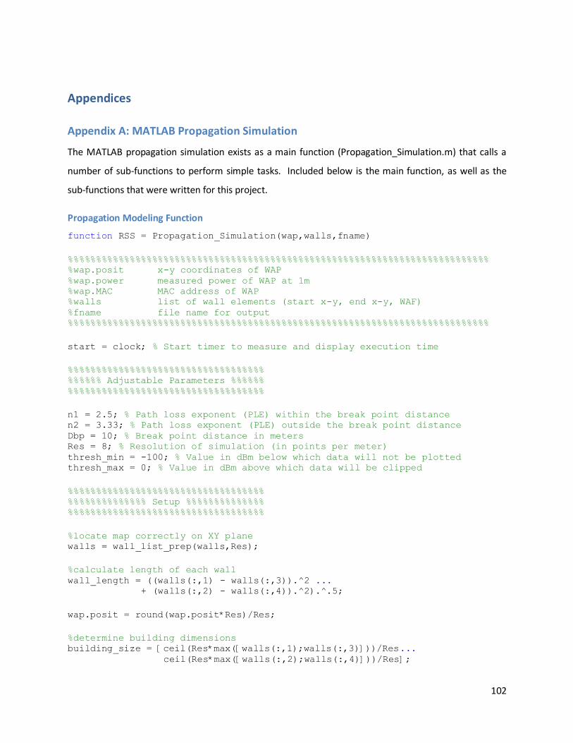
102
Appendices
Appendix A: MATLAB Propagation Simulation
The MATLAB propagation simulation exists as a main function (Propagation_Simulation.m) that calls a
number of sub-functions to perform simple tasks. Included below is the main function, as well as the
sub-functions that were written for this project.
Propagation Modeling Function
function RSS = Propagation_Simulation(wap,walls,fname)
%%%%%%%%%%%%%%%%%%%%%%%%%%%%%%%%%%%%%%%%%%%%%%%%%%%%%%%%%%%%%%%%%%%%%%%%%%% %wap.posit x-y coordinates of WAP %wap.power measured power of WAP at 1m %wap.MAC MAC address of WAP %walls list of wall elements (start x-y, end x-y, WAF) %fname file name for output %%%%%%%%%%%%%%%%%%%%%%%%%%%%%%%%%%%%%%%%%%%%%%%%%%%%%%%%%%%%%%%%%%%%%%%%%%%
start = clock; % Start timer to measure and display execution time
%%%%%%%%%%%%%%%%%%%%%%%%%%%%%%%%%%% %%%%%% Adjustable Parameters %%%%%% %%%%%%%%%%%%%%%%%%%%%%%%%%%%%%%%%%%
n1 = 2.5; % Path loss exponent (PLE) within the break point distance n2 = 3.33; % Path loss exponent (PLE) outside the break point distance Dbp = 10; % Break point distance in meters Res = 8; % Resolution of simulation (in points per meter) thresh_min = -100; % Value in dBm below which data will not be plotted thresh_max = 0; % Value in dBm above which data will be clipped
%%%%%%%%%%%%%%%%%%%%%%%%%%%%%%%%%%% %%%%%%%%%%%%%% Setup %%%%%%%%%%%%%% %%%%%%%%%%%%%%%%%%%%%%%%%%%%%%%%%%%
%locate map correctly on XY plane walls = wall_list_prep(walls,Res);
%calculate length of each wall wall_length = ((walls(:,1) - walls(:,3)).^2 ... + (walls(:,2) - walls(:,4)).^2).^.5;
wap.posit = round(wap.posit*Res)/Res;
%determine building dimensions building_size = [ceil(Res*max([walls(:,1);walls(:,3)]))/Res... ceil(Res*max([walls(:,2);walls(:,4)]))/Res];
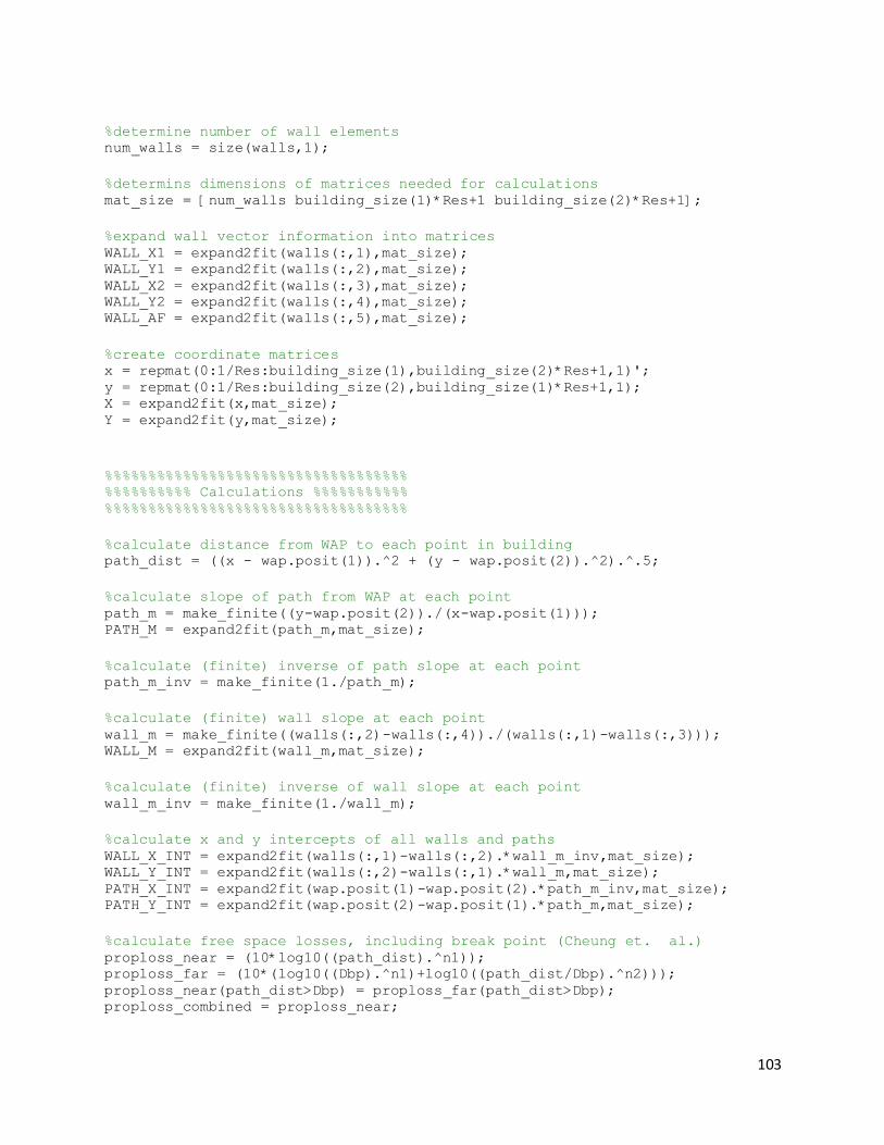
103
%determine number of wall elements num_walls = size(walls,1);
%determins dimensions of matrices needed for calculations mat_size = [num_walls building_size(1)*Res+1 building_size(2)*Res+1];
%expand wall vector information into matrices WALL_X1 = expand2fit(walls(:,1),mat_size); WALL_Y1 = expand2fit(walls(:,2),mat_size); WALL_X2 = expand2fit(walls(:,3),mat_size); WALL_Y2 = expand2fit(walls(:,4),mat_size); WALL_AF = expand2fit(walls(:,5),mat_size);
%create coordinate matrices x = repmat(0:1/Res:building_size(1),building_size(2)*Res+1,1)'; y = repmat(0:1/Res:building_size(2),building_size(1)*Res+1,1); X = expand2fit(x,mat_size); Y = expand2fit(y,mat_size);
%%%%%%%%%%%%%%%%%%%%%%%%%%%%%%%%%%% %%%%%%%%%% Calculations %%%%%%%%%%% %%%%%%%%%%%%%%%%%%%%%%%%%%%%%%%%%%%
%calculate distance from WAP to each point in building path_dist = ((x - wap.posit(1)).^2 + (y - wap.posit(2)).^2).^.5;
%calculate slope of path from WAP at each point path_m = make_finite((y-wap.posit(2))./(x-wap.posit(1))); PATH_M = expand2fit(path_m,mat_size);
%calculate (finite) inverse of path slope at each point path_m_inv = make_finite(1./path_m);
%calculate (finite) wall slope at each point wall_m = make_finite((walls(:,2)-walls(:,4))./(walls(:,1)-walls(:,3))); WALL_M = expand2fit(wall_m,mat_size);
%calculate (finite) inverse of wall slope at each point wall_m_inv = make_finite(1./wall_m);
%calculate x and y intercepts of all walls and paths WALL_X_INT = expand2fit(walls(:,1)-walls(:,2).*wall_m_inv,mat_size); WALL_Y_INT = expand2fit(walls(:,2)-walls(:,1).*wall_m,mat_size); PATH_X_INT = expand2fit(wap.posit(1)-wap.posit(2).*path_m_inv,mat_size); PATH_Y_INT = expand2fit(wap.posit(2)-wap.posit(1).*path_m,mat_size);
%calculate free space losses, including break point (Cheung et. al.) proploss_near = (10*log10((path_dist).^n1)); proploss_far = (10*(log10((Dbp).^n1)+log10((path_dist/Dbp).^n2))); proploss_near(path_dist>Dbp) = proploss_far(path_dist>Dbp); proploss_combined = proploss_near;
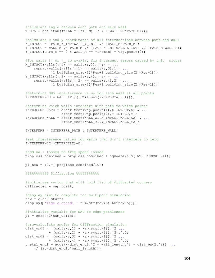
104
%calculate angle between each path and each wall THETA = abs(atan((WALL_M-PATH_M) ./ ( 1+WALL_M.*PATH_M)));
%calculate x and y coordinates of all intersections between path and wall X_INTSCT = (PATH_Y_INT-WALL_Y_INT) ./ (WALL_M-PATH_M); Y_INTSCT = WALL_M .* PATH_M .* (PATH_X_INT-WALL_X_INT) ./ (PATH_M-WALL_M); Y_INTSCT(PATH_M == 0 & WALL_M == -intmax) = wap.posit(2);
%for walls || or |_ to x-axis, fix intercept errors caused by inf. slopes X_INTSCT(walls(:,1) == walls(:,3),:,:) = ... repmat(walls(walls(:,1) == walls(:,3),1), ... [1 building_size(1)*Res+1 building_size(2)*Res+1]); Y_INTSCT(walls(:,2) == walls(:,4),:,:) = ... repmat(walls(walls(:,2) == walls(:,4),2), ... [1 building_size(1)*Res+1 building_size(2)*Res+1]);
%determine dBm interference value for each wall at all points INTERFERENCE = WALL_AF./(.5*(1+max(sin(THETA),.1)));
%determine which walls interfere with path to which points INTERFERE_PATH = order_test(wap.posit(1),X_INTSCT,X) & ... order_test(wap.posit(2),Y_INTSCT,Y); INTERFERE_WALL = order_test(WALL_X1,X_INTSCT,WALL_X2) & ... order_test(WALL_Y1,Y_INTSCT,WALL_Y2);
INTERFERE = INTERFERE_PATH & INTERFERE_WALL;
%set interference values for walls that don't interfere to zero INTERFERENCE(~INTERFERE)=0;
%add wall losses to free space losses proploss_combined = proploss_combined + squeeze(sum(INTERFERENCE,1));
pl_new = 10.^(-proploss_combined/10);
%%%%%%%%%%% Diffraction %%%%%%%%%%%
%initialize vector that will hold list of diffracted corners diffracted = wap.posit;
%display time to complete non multipath simulation now = clock-start; display(['Time elapsed: ' num2str(now(6)+60*now(5))])
%initialize variable for WAP to edge pathlosses pl = zeros(2*num_walls);
%pre-calculate angles for diffraction simulation dist_end1 = ((walls(:,1) - wap.posit(1)).^2 ... + (walls(:,2) - wap.posit(2)).^2).^.5; dist_end2 = ((walls(:,3) - wap.posit(1)).^2 ... + (walls(:,4) - wap.posit(2)).^2).^.5; theta1_end1 = acos(((dist_end1.^2 + wall_length.^2 - dist_end2.^2)) ... ./ (2.*dist_end1.*wall_length));
105
theta1_end2 = acos(((dist_end2.^2 + wall_length.^2 - dist_end1.^2)) ... ./ (2.*dist_end2.*wall_length));
%loop to test for diffraction at each end of each wall for i = 1:2*num_walls
%determine which wall of which end to test wall = ceil(i/2); wall_end = mod(i+1,2)+1;
%determine whether or not wall end is a corner for diffraction [will_diffract diffracted] = ... is_corner(walls,wall,wall_end,wap.posit,Res,diffracted);
%if point is corner at which diffract will occur if will_diffract
%get x and y coord. of wall ends plx = walls(wall,2*mod(i+1,2)+1); ply = walls(wall,2*mod(i+1,2)+2); plx_alt = walls(wall,2*mod(i,2)+1); ply_alt = walls(wall,2*mod(i,2)+2);
%get proploss from WAP to wall end pl(i)=proploss_combined(plx*Res+1,ply*Res+1);
%get distance from WAP to both wall ends path_dist = ((x - plx).^2 + (y - ply).^2).^.5; path_dist_alt = ((x - plx_alt).^2 + (y - ply_alt).^2).^.5;
%calculate slope of path from WAP at each point path_m = make_finite((y-ply)./(x-plx)); PATH_M = expand2fit(path_m,mat_size);
%calculate (finite) inverse of path slope at each point path_m_inv = make_finite(1./path_m);
%calculate x and y intercepts of paths PATH_X_INT = expand2fit(plx-ply.*path_m_inv,mat_size); PATH_Y_INT = expand2fit(ply-plx.*path_m,mat_size);
%calculate free space losses proploss2 = (10*log10((path_dist).^n1)); proploss_far = (10*(log10((Dbp).^n1)+log10((path_dist/Dbp).^n2))); proploss2(path_dist>Dbp) = proploss_far(path_dist>Dbp); proploss2 = make_finite(proploss2);
%calculate angle between each path and each wall THETA = atan((WALL_M-PATH_M) ./ ( 1+WALL_M.*PATH_M));
%get/calculate angles needed to calculate diffraction coefficient theta_1 = eval(['theta1_end' num2str(wall_end)]); theta_1 = abs(theta_1(wall)); theta_2 = acos((path_dist.^2 + wall_length(wall).^2 ...
106
- path_dist_alt.^2) ... ./ (2.*path_dist.*wall_length(wall))); theta_2 = theta_2.*(-1).^(squeeze(INTERFERE_PATH(wall,:,:))-1); theta_2 = 2*pi - mod(real(theta_2),2*pi);
%calculate x and y coord. of intersections between path and wall X_INTSCT = (PATH_Y_INT-WALL_Y_INT) ./ (WALL_M-PATH_M); Y_INTSCT = WALL_M .* PATH_M .* ... (PATH_X_INT-WALL_X_INT) ./ (PATH_M-WALL_M);
%for walls || or |_ to x-axis, correct inf. slope errors X_INTSCT(walls(:,1) == walls(:,3),:,:) = ... repmat(walls(walls(:,1) == walls(:,3),1), ... [1 building_size(1)*Res+1 building_size(2)*Res+1]); Y_INTSCT(walls(:,2) == walls(:,4),:,:) = ... repmat(walls(walls(:,2) == walls(:,4),2), ... [1 building_size(1)*Res+1 building_size(2)*Res+1]);
%determine dBm interference value for each wall at all points INTERFERENCE = make_finite(WALL_AF./max(sin(abs(THETA)),.1));
%determine which walls interfere with path to which points INTERFERE = order_test(plx,X_INTSCT,X) & ... order_test(ply,Y_INTSCT,Y) & ... order_test(WALL_X1,X_INTSCT,WALL_X2) & ... order_test(WALL_Y1,Y_INTSCT,WALL_Y2);
%set interference values for walls that don't interfere to zero INTERFERENCE(~INTERFERE)=0;
%add wall losses to free space losses proploss2 = proploss2 + squeeze(sum(INTERFERENCE,1));
%calculate diffraction coefficient D = squeeze(abs(-exp(-j*pi/4)/sqrt(2*pi) ... .*abs(csc(theta_2-theta_1)) ... .*sqrt(-sin(theta_2)./sin(theta_1))));
%remove infinite and unnecessary values from array D(D==Inf | D==-Inf | isnan(D) | theta_2<=pi) = ... zeros(size(D(D==Inf | D==-Inf | isnan(D) | theta_2<=pi))); D(D>1) = zeros(size(D(D>1))); D(D<0) = zeros(size(D(D>1)));
%calculate, correct, and add new pathlosses to running total pl_tmp = 10.^(-pl(i)/10)*10.^(-proploss2/10).*D; pl_tmp(isnan(pl_tmp)) = zeros(size(pl_tmp(isnan(pl_tmp)))); pl_new = pl_new + (pl_tmp);
%display progress and time elapsed disp([num2str(i) ' of ' num2str(2*num_walls) ' complete']) now = clock-start; display(['Time elapsed: ' num2str(now(6)+60*now(5)) ' seconds']) end
107
end
%convert proploss to decibels proploss = -10*log10(pl_new);
%subtract propagation losses from transmit power RSS = wap.power - real(proploss);
%remove low values to preserve plot scale RSS(RSS>thresh_max) = thresh_max;
%clip high values to preserve plot scale RSS(RSS<thresh_min) = thresh_min;
%%%%%%%%%%%%%%%%%%%%%%%%%%%%%%%%%%% %%%%%%%%%%% Plot Results %%%%%%%%%% %%%%%%%%%%%%%%%%%%%%%%%%%%%%%%%%%%%
[TMP RSS] = down_sample(RSS); %downsample array to output resolution
%call function to plot results SS_plot(building_size,walls,RSS,diffracted)
%open file and save results fid = fopen([fname '.txt'],'w'); fprintf(fid,'%12s\n',wap.MAC); fprintf(fid,'%8.0f%8.0f\n',size(RSS)); format = [repmat('%8.2f',1,size(RSS,2)) '\n']; fprintf(fid,format,fliplr(RSS')); fclose(fid);
%clear variables from memory clear all
return
Supporting Functions
The following functions, listed in the order they are called, perform tasks subordinate to the propagation
simulation.
wall_list_prep.m
%This function translates wall position data to the origin and rounds %coordinate to the nearest multiple of a given resolution function wall_list_new = wall_list_prep(walls,Res)
%%%%%%%%%%%%%%%%%%%%%%%%%%%%%%%%%%%%%%%%%%%%%%%%%%%%%%%%%%%%%%%%%%%%%%%%%%% %walls list of wall element coordinates (start x-y, end x-y) %Res Resolution of model (in m^-1) %%%%%%%%%%%%%%%%%%%%%%%%%%%%%%%%%%%%%%%%%%%%%%%%%%%%%%%%%%%%%%%%%%%%%%%%%%%
108
%round values to nearest multiple of resolution walls(:,1:4) = round(walls(:,1:4)*Res)/Res;
%find coordinates of wall point closest to origin xmin = min([walls(:,1);walls(:,2)]); ymin = min([walls(:,2);walls(:,4)]);
%translate coordinates to match closest corner to origin walls(:,1) = walls(:,1)-xmin; walls(:,3) = walls(:,3)-xmin; walls(:,2) = walls(:,2)-ymin; walls(:,4) = walls(:,4)-ymin;
%return new wall list wall_list_new = walls;
return
expand2fit.m
%This function expands vectors and arrays into the 3-d form used for matrix %calculations function out = expand2fit(in,fit_size)
%%%%%%%%%%%%%%%%%%%%%%%%%%%%%%%%%%%%%%%%%%%%%%%%%%%%%%%%%%%%%%%%%%%%%%%%%%% %in input vector %Res size required to array operations %%%%%%%%%%%%%%%%%%%%%%%%%%%%%%%%%%%%%%%%%%%%%%%%%%%%%%%%%%%%%%%%%%%%%%%%%%%
%seperate fit vector dimensions x = fit_size(1); y = fit_size(2); z = fit_size(3);
%if input is a vector if size(in) == [x 1] %repeat in two additional dimensions out = repmat(in,[1 y z]);
%else if input is an array elseif size(in) == [y z] %repeat in one additional dimension out = repmat(reshape(in,[1 y z]),[x 1 1]);
%if input is of invalid size, return an error else out = zeros(x,y,z); error('Invalid input to function "expand2fit"') end
return
make_finite.m
%replaces infinite values with the maximum integer value of the system
109
function y = make_finite(x)
%%%%%%%%%%%%%%%%%%%%%%%%%%%%%%%%%%%%%%%%%%%%%%%%%%%%%%%%%%%%%%%%%%%%%%%%%%% %x input vector to be made finite %%%%%%%%%%%%%%%%%%%%%%%%%%%%%%%%%%%%%%%%%%%%%%%%%%%%%%%%%%%%%%%%%%%%%%%%%%%
%replace all infinite values with maximum integer of corresponding sign x(x==Inf)=intmax; x(x==-Inf)=-intmax;
%return result y=x;
return
order_test.m
%determines if the B input is between the A and C inputs, inclusive function bool = order_test(a, b, c)
%%%%%%%%%%%%%%%%%%%%%%%%%%%%%%%%%%%%%%%%%%%%%%%%%%%%%%%%%%%%%%%%%%%%%%%%%%% %a first extreme value %b test value %c second extreme value %%%%%%%%%%%%%%%%%%%%%%%%%%%%%%%%%%%%%%%%%%%%%%%%%%%%%%%%%%%%%%%%%%%%%%%%%%%
%round values to nearest thousandth (tollerence) a = round(10^3*a)/10^3; b = round(10^3*b)/10^3; c = round(10^3*c)/10^3;
%perform logical comparison bool = (a<=b&b<=c) | (a>=b&b>=c);
return
is_corner.m
%This function searchs a list of walls for intersections with a given wall %in order to determine if a corner shape exists that would cause %significant diffraction function [is diffract] = is_corner(walls,wall,end_in,wap_xy,Res,diffract)
%%%%%%%%%%%%%%%%%%%%%%%%%%%%%%%%%%%%%%%%%%%%%%%%%%%%%%%%%%%%%%%%%%%%%%%%%%% %walls list of wall element coordinates (start x-y, end x-y) %wall specific wall to be checked for intersections %end_in which end of specific wall to check for corners %wap_xy x-y coordinates of wireless access point %Res resolution of simulation %diffract list of already found corners to which any newfound corners % will be appended %%%%%%%%%%%%%%%%%%%%%%%%%%%%%%%%%%%%%%%%%%%%%%%%%%%%%%%%%%%%%%%%%%%%%%%%%%%
%assume that the end being tested is a corner is = 1;
110
%reshape walls array into a list of ends ends = [walls(:,1:2) ; walls(:,3:4)];
%pre-allocate memory for intersection-count variable k = zeros(length(ends),1);
%for each end of a wall for i = 1:length(ends) %determine if coordinates are the same as end of another wall if isequal(ends((end_in-1)*length(walls)+wall,:),ends(i,:)) %if coordinates are the same, set corresponding count bit to '1' k(i)=1; end %if more than one overlap (in addition to overlap with self) %is found, break out of loop if sum(k) > 2 break end end
%set count bit corresponding to overlap with self back to '0' k((end_in-1)*length(walls)+wall)=0;
%if an intersection exists if sum(k) %This section of code determines the orientation, relative to an %incident signal path, of a corner formed by two walls with overlapping %ends. Diffraction will ot occur at corners to which the path is %incident on the inside. end_1 = end_in; end_2 = 1+(find(squeeze(k),1)>length(walls)); wall_1_1 = walls(wall,1+2*(end_1-1):2+2*(end_1-1)); wall_1_2 = walls(wall,3-2*(end_1-1):4-2*(end_1-1)); wall_1_d = [wall_1_1(1) - wall_1_2(1) wall_1_1(2) - wall_1_2(2)]; wall_1_l = sum((wall_1_1-wall_1_2).^2)^.5; wall_1_test = wall_1_1-(1/Res).*wall_1_d./wall_1_l; wall_2_1 = walls(mod(find(k,1)-1,length(walls))+1, ... 1+2*(end_2-1):2+2*(end_2-1)); wall_2_2 = walls(mod(find(k,1)-1,length(walls))+1, ... 3-2*(end_2-1):4-2*(end_2-1)); wall_2_d = [wall_2_1(1) - wall_2_2(1) wall_2_1(2) - wall_2_2(2)]; wall_2_l = sum((wall_2_1-wall_2_2).^2)^.5; wall_2_test = wall_2_1-(1/Res).*wall_2_d./wall_2_l; dist_1_1 = sum((wall_1_1-wap_xy).^2)^.5; dist_1_test = sum((wall_1_test-wap_xy).^2)^.5; dist_2_1 = sum((wall_2_1-wap_xy).^2)^.5; dist_2_test = sum((wall_2_test-wap_xy).^2)^.5; away_1 = (dist_1_test > dist_1_1); away_2 = (dist_2_test > dist_2_1); if ~xor(away_1,away_2) is = 0; end
%otherwise, check for 'T' shaped intersections that will prevent %diffraction
111
else for i = 1:length(walls) d1=((walls(i,1)-walls(wall,1+2*(end_in-1)))^2+(walls(i,2) ... -walls(wall,2+2*(end_in-1)))^2)^.5; d2=((walls(i,3)-walls(wall,1+2*(end_in-1)))^2+(walls(i,4) ... -walls(wall,2+2*(end_in-1)))^2)^.5; wall_length=((walls(i,1)-walls(i,3))^2+ ... (walls(i,2)-walls(i,4))^2)^.5; if ((d1+d2) == wall_length) && (i ~= wall) is = 0; break end end end
%if no conditions found that prevent diffraction if is == 1 %append location of corner to list of corners and return diffract = [diffract; walls(wall,1+2*(end_in-1):2+2*(end_in-1))]; end
return
down_sample.m
%This function downsamples an array of predicted values to a size that is %computationally appropriate for manipulation on the HTC Hero function [y1 y2] = down_sample(x)
%%%%%%%%%%%%%%%%%%%%%%%%%%%%%%%%%%%%%%%%%%%%%%%%%%%%%%%%%%%%%%%%%%%%%%%%%%% %x oversampled array to be reduced %%%%%%%%%%%%%%%%%%%%%%%%%%%%%%%%%%%%%%%%%%%%%%%%%%%%%%%%%%%%%%%%%%%%%%%%%%%
%filtering array for use in averaging; oversampled points that map to %multiple daownsampled points are weighted lower for each use remap = [1 2 2 2 1; ... 2 4 4 4 2; ... 2 4 4 4 2; ... 2 4 4 4 2; ... 1 2 2 2 1];
%for each element of the desired downsampled array for i = 1:round(size(x,1)/2)/2 for j = 1:round(size(x,2)/2)/2 if 4*i-3 < size(x,1) && 4*j-3 < size(x,2) y1(i,j) = x(4*i-3,4*j-3); end
%create indexing array of coordinate to correctly apply filtering % array coordx_tmp = [4*i-5 4*i-4 4*i-3 4*i-2 4*i-1; ... 4*i-5 4*i-4 4*i-3 4*i-2 4*i-1; ... 4*i-5 4*i-4 4*i-3 4*i-2 4*i-1; ... 4*i-5 4*i-4 4*i-3 4*i-2 4*i-1; ... 4*i-5 4*i-4 4*i-3 4*i-2 4*i-1]; coordy_tmp = [4*j-5 4*j-5 4*j-5 4*j-5 4*j-5; ...
112
4*j-4 4*j-4 4*j-4 4*j-4 4*j-4; ... 4*j-3 4*j-3 4*j-3 4*j-3 4*j-3; ... 4*j-2 4*j-2 4*j-2 4*j-2 4*j-2; ... 4*j-1 4*j-1 4*j-1 4*j-1 4*j-1];
%only use indices for which elements exist coordx = coordx_tmp(coordx_tmp>0 & coordx_tmp<=size(x,1) ... & coordy_tmp>0 & coordy_tmp<=size(x,2)); coordy = coordy_tmp(coordx_tmp>0 & coordx_tmp<=size(x,1) ... & coordy_tmp>0 & coordy_tmp<=size(x,2)); x_rel = diag(x(coordx,coordy));
%collect relevant signal strength values remap_rel = remap(coordx_tmp>0 & coordx_tmp<=size(x,1) ... & coordy_tmp>0 & coordy_tmp<=size(x,2));
%perform weighted average using relative remap array elements y2(i,j) = sum(sum(x_rel.*remap_rel))/sum(sum(remap_rel)); end end
return
SS_plot.m
%This function plots the output of the propagation simulation function function SS_plot(building_size,wall_list,RSS,diffracted)
%%%%%%%%%%%%%%%%%%%%%%%%%%%%%%%%%%%%%%%%%%%%%%%%%%%%%%%%%%%%%%%%%%%%%%%%%%% %building_size dimensions of building being modeled %wall_list list of wall elements used to plot building layout %RSS array of predicted received signal strength values %diffracted list of coordinate of corners at which diffraction was % modeled %%%%%%%%%%%%%%%%%%%%%%%%%%%%%%%%%%%%%%%%%%%%%%%%%%%%%%%%%%%%%%%%%%%%%%%%%%%
%open a new figure figure
%in the right subplot, plot the predicted RSS values subplot(1,2,2) imagesc(0:.1:building_size(2),0:.1:building_size(1),RSS); title('RSS (dBm)') xlabel('meters') ylabel('meters') grid off,axis tight,axis equal,axis vis3d,view([0 90]),zoom(1),colorbar,axis
xy axis([min([wall_list(:,2) ; wall_list(:,4)]) ... max([wall_list(:,2) ; wall_list(:,4)]) ... min([wall_list(:,1) ; wall_list(:,3)]) ... max([wall_list(:,1) ; wall_list(:,3)])])
%in the left subplot, plot the building layout includig walls, WAP % location, and location of corners for which diffraction was modeled subplot(1,2,1)
113
title('Floor Plan') xlabel('meters') ylabel('meters') line([wall_list(:,2) wall_list(:,4)]',[wall_list(:,1)
wall_list(:,3)]','color','b') axis equal,axis tight,zoom(1) axis([min([wall_list(:,2) ; wall_list(:,4)]) ... max([wall_list(:,2) ; wall_list(:,4)]) ... min([wall_list(:,1) ; wall_list(:,3)]) ... max([wall_list(:,1) ; wall_list(:,3)])]) axis xy hold on plot(diffracted(1,2),diffracted(1,1),'xr') plot(diffracted(2:end,2),diffracted(2:end,1),'og')
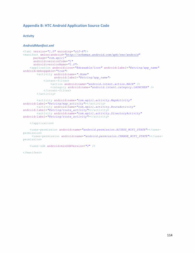
114
Appendix B: HTC Android Application Source Code
Activity
AndroidManifest.xml
<?xml version="1.0" encoding="utf-8"?>
<manifest xmlns:android="http://schemas.android.com/apk/res/android"
package="com.wpirl"
android:versionCode="1"
android:versionName="1.0">
<application android:icon="@drawable/icon" android:label="@string/app_name"
android:debuggable="true">
<activity android:name=".Home"
android:label="@string/app_name">
<intent-filter>
<action android:name="android.intent.action.MAIN" />
<category android:name="android.intent.category.LAUNCHER" />
</intent-filter>
</activity>
<activity android:name="com.wpirl.activity.MapActivity"
android:label="@string/map_activity"></activity>
<activity android:name="com.wpirl.activity.RouteActivity"
android:label="@string/route_activity"></activity>
<activity android:name="com.wpirl.activity.DirectoryActivity"
android:label="@string/route_activity"></activity>
</application>
<uses-permission android:name="android.permission.ACCESS_WIFI_STATE"></uses-
permission>
<uses-permission android:name="android.permission.CHANGE_WIFI_STATE"></uses-
permission>
<uses-sdk android:minSdkVersion="3" />
</manifest>
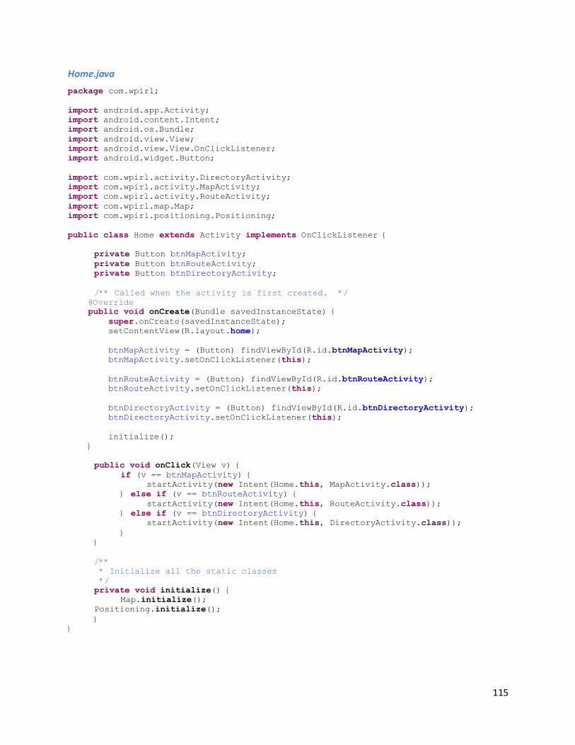
115
Home.java
package com.wpirl;
import android.app.Activity;
import android.content.Intent;
import android.os.Bundle;
import android.view.View;
import android.view.View.OnClickListener;
import android.widget.Button;
import com.wpirl.activity.DirectoryActivity;
import com.wpirl.activity.MapActivity;
import com.wpirl.activity.RouteActivity;
import com.wpirl.map.Map;
import com.wpirl.positioning.Positioning;
public class Home extends Activity implements OnClickListener {
private Button btnMapActivity;
private Button btnRouteActivity;
private Button btnDirectoryActivity;
/** Called when the activity is first created. */
@Override
public void onCreate(Bundle savedInstanceState) {
super.onCreate(savedInstanceState);
setContentView(R.layout.home);
btnMapActivity = (Button) findViewById(R.id.btnMapActivity);
btnMapActivity.setOnClickListener(this);
btnRouteActivity = (Button) findViewById(R.id.btnRouteActivity);
btnRouteActivity.setOnClickListener(this);
btnDirectoryActivity = (Button) findViewById(R.id.btnDirectoryActivity);
btnDirectoryActivity.setOnClickListener(this);
initialize();
}
public void onClick(View v) {
if (v == btnMapActivity) {
startActivity(new Intent(Home.this, MapActivity.class));
} else if (v == btnRouteActivity) {
startActivity(new Intent(Home.this, RouteActivity.class));
} else if (v == btnDirectoryActivity) {
startActivity(new Intent(Home.this, DirectoryActivity.class));
}
}
/**
* Initialize all the static classes
*/
private void initialize() {
Map.initialize();
Positioning.initialize();
}
}
116
Home.xlm
<?xml version="1.0" encoding="utf-8"?>
<LinearLayout xmlns:android="http://schemas.android.com/apk/res/android"
android:orientation="vertical"
android:layout_width="fill_parent"
android:layout_height="fill_parent"
>
<Button
android:layout_width="fill_parent"
android:layout_height="wrap_content"
android:id="@+id/btnMapActivity"
android:text="@string/map_activity"/>
<Button
android:layout_width="fill_parent"
android:layout_height="wrap_content"
android:id="@+id/btnRouteActivity"
android:text="@string/route_activity"/>
<Button
android:layout_width="fill_parent"
android:layout_height="wrap_content"
android:id="@+id/btnDirectoryActivity"
android:text="@string/directory_activity"/>
</LinearLayout>
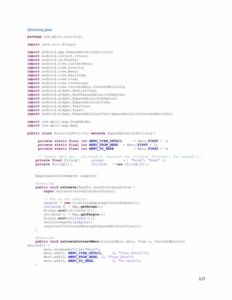
117
Directory.java
package com.wpirl.activity;
import java.util.Arrays;
import android.app.ExpandableListActivity;
import android.content.Intent;
import android.os.Bundle;
import android.view.ContextMenu;
import android.view.Gravity;
import android.view.Menu;
import android.view.MenuItem;
import android.view.View;
import android.view.ViewGroup;
import android.view.ContextMenu.ContextMenuInfo;
import android.widget.AbsListView;
import android.widget.BaseExpandableListAdapter;
import android.widget.ExpandableListAdapter;
import android.widget.ExpandableListView;
import android.widget.TextView;
import android.widget.Toast;
import android.widget.ExpandableListView.ExpandableListContextMenuInfo;
import com.wpirl.map.GraphNode;
import com.wpirl.map.Map;
public class DirectoryActivity extends ExpandableListActivity {
private static final int MENU_VIEW_DETAIL = Menu.FIRST + 1;
private static final int MENU_FROM_HERE = Menu.FIRST + 2;
private static final int MENU_TO_HERE = Menu.FIRST + 3;
// Sample data set. children[i] contains the children (String[]) for groups[i].
private final String[] groups = { "Room", "Name" };
private String[][] children = new String[2][];
ExpandableListAdapter adapter;
@Override
public void onCreate(Bundle savedInstanceState) {
super.onCreate(savedInstanceState);
// Set up our adapter
adapter = new DirectoryExpandableListAdapter();
children[0] = Map.getRooms();
Arrays.sort(children[0]);
children[1] = Map.getPeople();
Arrays.sort(children[1]);
setListAdapter(adapter);
registerForContextMenu(getExpandableListView());
}
@Override
public void onCreateContextMenu(ContextMenu menu, View v, ContextMenuInfo
menuInfo) {
menu.setHeaderTitle("Menu");
menu.add(0, MENU_VIEW_DETAIL, 0, "View Detail");
menu.add(0, MENU_FROM_HERE, 0, "From Here");
menu.add(0, MENU_TO_HERE, 0, "To Here");
}
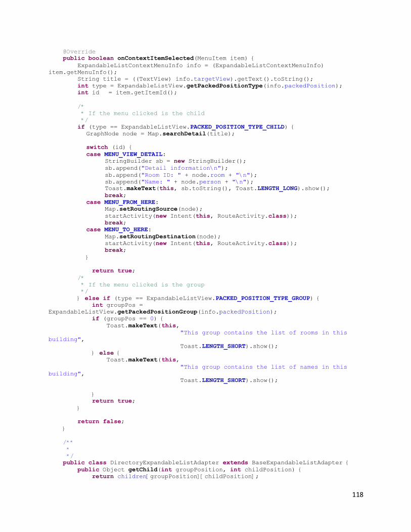
118
@Override
public boolean onContextItemSelected(MenuItem item) {
ExpandableListContextMenuInfo info = (ExpandableListContextMenuInfo)
item.getMenuInfo();
String title = ((TextView) info.targetView).getText().toString();
int type = ExpandableListView.getPackedPositionType(info.packedPosition);
int id = item.getItemId();
/*
* If the menu clicked is the child
*/
if (type == ExpandableListView.PACKED_POSITION_TYPE_CHILD) {
GraphNode node = Map.searchDetail(title);
switch (id) {
case MENU_VIEW_DETAIL:
StringBuilder sb = new StringBuilder();
sb.append("Detail information\n");
sb.append("Room ID: " + node.room + "\n");
sb.append("Name: " + node.person + "\n");
Toast.makeText(this, sb.toString(), Toast.LENGTH_LONG).show();
break;
case MENU_FROM_HERE:
Map.setRoutingSource(node);
startActivity(new Intent(this, RouteActivity.class));
break;
case MENU_TO_HERE:
Map.setRoutingDestination(node);
startActivity(new Intent(this, RouteActivity.class));
break;
}
return true;
/*
* If the menu clicked is the group
*/
} else if (type == ExpandableListView.PACKED_POSITION_TYPE_GROUP) {
int groupPos =
ExpandableListView.getPackedPositionGroup(info.packedPosition);
if (groupPos == 0) {
Toast.makeText( this,
"This group contains the list of rooms in this
building",
Toast.LENGTH_SHORT).show();
} else {
Toast.makeText( this,
"This group contains the list of names in this
building",
Toast.LENGTH_SHORT).show();
}
return true;
}
return false;
}
/**
*
*/
public class DirectoryExpandableListAdapter extends BaseExpandableListAdapter {
public Object getChild(int groupPosition, int childPosition) {
return children[groupPosition][childPosition];
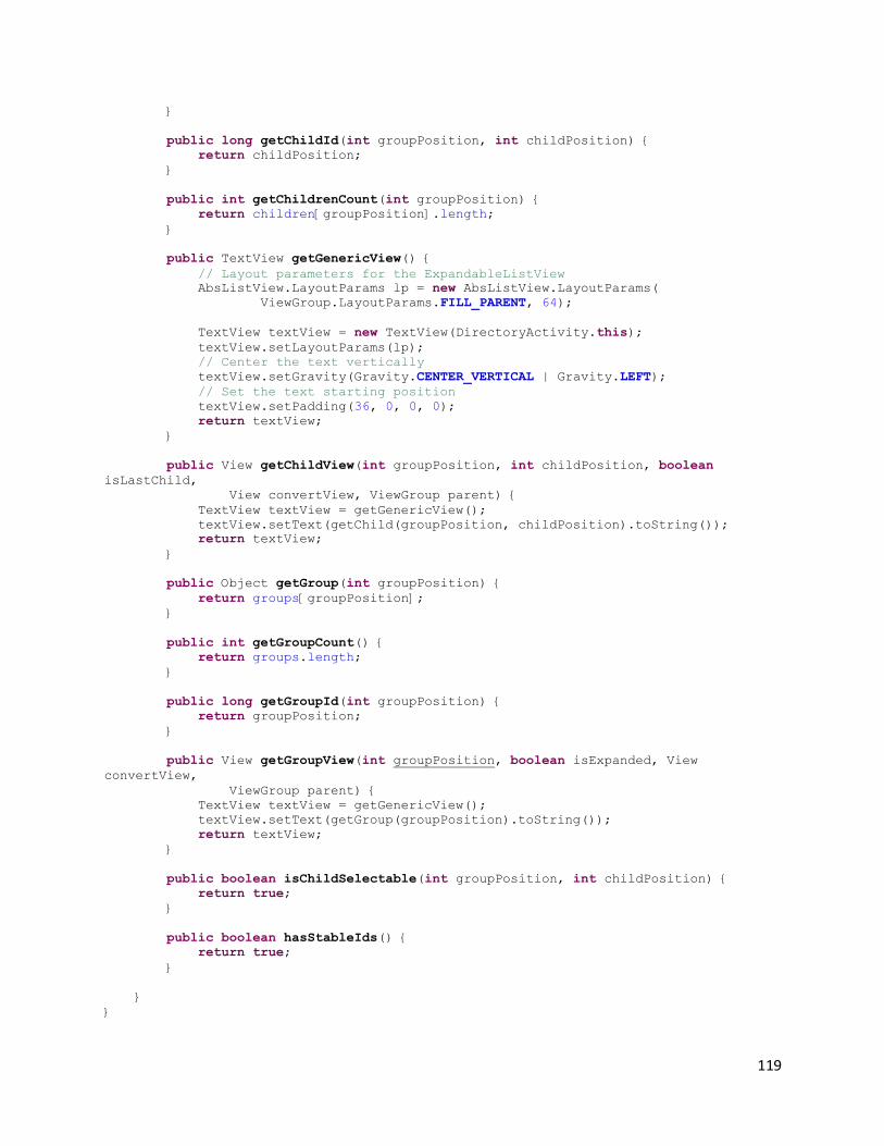
119
}
public long getChildId(int groupPosition, int childPosition) {
return childPosition;
}
public int getChildrenCount(int groupPosition) {
return children[groupPosition].length;
}
public TextView getGenericView() {
// Layout parameters for the ExpandableListView
AbsListView.LayoutParams lp = new AbsListView.LayoutParams(
ViewGroup.LayoutParams.FILL_PARENT, 64);
TextView textView = new TextView(DirectoryActivity.this);
textView.setLayoutParams(lp);
// Center the text vertically
textView.setGravity(Gravity.CENTER_VERTICAL | Gravity.LEFT);
// Set the text starting position
textView.setPadding(36, 0, 0, 0);
return textView;
}
public View getChildView(int groupPosition, int childPosition, boolean
isLastChild,
View convertView, ViewGroup parent) {
TextView textView = getGenericView();
textView.setText(getChild(groupPosition, childPosition).toString());
return textView;
}
public Object getGroup(int groupPosition) {
return groups[groupPosition];
}
public int getGroupCount() {
return groups.length;
}
public long getGroupId(int groupPosition) {
return groupPosition;
}
public View getGroupView(int groupPosition, boolean isExpanded, View
convertView,
ViewGroup parent) {
TextView textView = getGenericView();
textView.setText(getGroup(groupPosition).toString());
return textView;
}
public boolean isChildSelectable(int groupPosition, int childPosition) {
return true;
}
public boolean hasStableIds() {
return true;
}
}
}
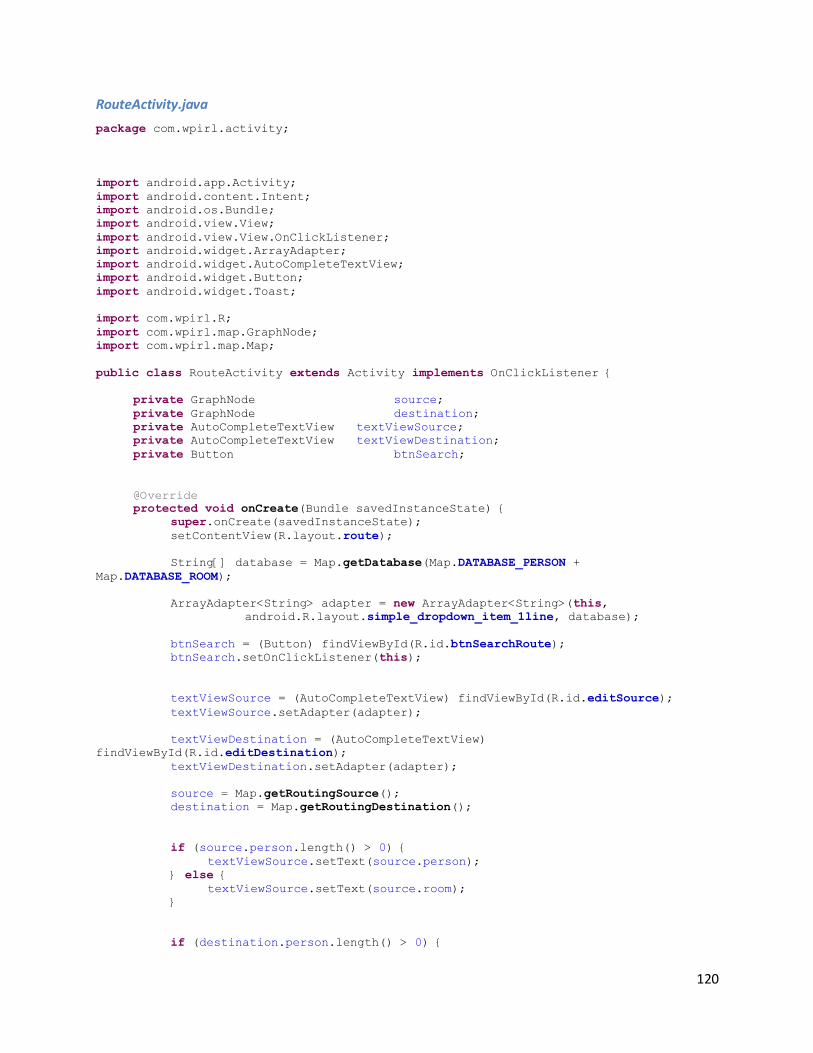
120
RouteActivity.java
package com.wpirl.activity;
import android.app.Activity;
import android.content.Intent;
import android.os.Bundle;
import android.view.View;
import android.view.View.OnClickListener;
import android.widget.ArrayAdapter;
import android.widget.AutoCompleteTextView;
import android.widget.Button;
import android.widget.Toast;
import com.wpirl.R;
import com.wpirl.map.GraphNode;
import com.wpirl.map.Map;
public class RouteActivity extends Activity implements OnClickListener {
private GraphNode source;
private GraphNode destination;
private AutoCompleteTextView textViewSource;
private AutoCompleteTextView textViewDestination;
private Button btnSearch;
@Override
protected void onCreate(Bundle savedInstanceState) {
super.onCreate(savedInstanceState);
setContentView(R.layout.route);
String[] database = Map.getDatabase(Map.DATABASE_PERSON +
Map.DATABASE_ROOM);
ArrayAdapter<String> adapter = new ArrayAdapter<String>(this,
android.R.layout.simple_dropdown_item_1line, database);
btnSearch = (Button) findViewById(R.id.btnSearchRoute);
btnSearch.setOnClickListener(this);
textViewSource = (AutoCompleteTextView) findViewById(R.id.editSource);
textViewSource.setAdapter(adapter);
textViewDestination = (AutoCompleteTextView)
findViewById(R.id.editDestination);
textViewDestination.setAdapter(adapter);
source = Map.getRoutingSource();
destination = Map.getRoutingDestination();
if (source.person.length() > 0) {
textViewSource.setText(source.person);
} else {
textViewSource.setText(source.room);
}
if (destination.person.length() > 0) {
121
textViewDestination.setText(destination.person);
} else {
textViewDestination.setText(destination.room);
}
}
@Override
public void onClick(View v) {
if (v == btnSearch) {
if (textViewSource.getText().length() == 0) {
Toast.makeText(this, "Please input source",
Toast.LENGTH_SHORT).show();
} else if (textViewDestination.getText().length() == 0) {
Toast.makeText(this, "Please input destination",
Toast.LENGTH_SHORT).show();
} else {
Map.setRoutingSource(Map.searchDetail(textViewSource.getText().toString()));
Map.setRoutingDestination(Map.searchDetail(textViewDestination.getText().toString
()));
Map.enableRouting();
startActivity(new Intent(this, MapActivity.class));
}
}
}
}
122
Route.xml
<?xml version="1.0" encoding="utf-8"?>
<LinearLayout xmlns:android="http://schemas.android.com/apk/res/android"
android:orientation="vertical"
android:layout_width="fill_parent"
android:layout_height="wrap_content">
<TextView
android:layout_width="wrap_content"
android:layout_height="wrap_content"
android:text="Get directions from source to destination" />
<LinearLayout
android:orientation="horizontal"
android:layout_width="fill_parent"
android:layout_height="wrap_content">
<TextView
android:layout_width="wrap_content"
android:layout_height="wrap_content"
android:text="Source" />
<AutoCompleteTextView android:id="@+id/editSource"
android:layout_width="fill_parent"
android:layout_height="wrap_content"/>
</LinearLayout>
<LinearLayout
android:orientation="horizontal"
android:layout_width="fill_parent"
android:layout_height="wrap_content">
<TextView
android:layout_width="wrap_content"
android:layout_height="wrap_content"
android:text="Destination" />
<AutoCompleteTextView android:id="@+id/editDestination"
android:layout_width="fill_parent"
android:layout_height="wrap_content"/>
</LinearLayout>
<Button
android:id="@+id/btnSearchRoute"
android:layout_width="fill_parent"
android:layout_height="wrap_content"
android:text="Search Maps" />
</LinearLayout>
123
MapActivity.java
package com.wpirl.activity;
import java.util.Arrays;
import java.util.List;
import android.app.Activity;
import android.content.BroadcastReceiver;
import android.content.Context;
import android.content.Intent;
import android.content.IntentFilter;
import android.hardware.Sensor;
import android.hardware.SensorEvent;
import android.hardware.SensorEventListener;
import android.hardware.SensorManager;
import android.net.wifi.ScanResult;
import android.net.wifi.WifiManager;
import android.os.Bundle;
import android.view.Menu;
import android.view.MenuItem;
import android.widget.Toast;
import com.wpirl.map.GraphEdge;
import com.wpirl.map.GraphNode;
import com.wpirl.map.Map;
import com.wpirl.positioning.DeviceSensor;
import com.wpirl.positioning.Positioning;
import com.wpirl.positioning.WifiPositioning;
import com.wpirl.util.DeviceWriter;
import com.wpirl.util.Util;
import com.wpirl.view.MapView;
public class MapActivity extends Activity implements SensorEventListener {
public static final int MENU_MY_LOCATION = Menu.FIRST + 1;
public static final int MENU_CHOOSE_DESTINATION = Menu.FIRST + 2;
public static final int MENU_STOP_RECORDING = Menu.FIRST + 3;
private MapView view;
private SensorManager mSensorManager;
private WifiManager mWifiManager;
private WifiReceiver mWifiReceiver;
private DeviceWriter out;
private long timezero = 0;
@Override
public void onCreate(Bundle savedInstanceState) {
super.onCreate(savedInstanceState);
view = new MapView(this);
setContentView(view);
mSensorManager = (SensorManager)getSystemService(SENSOR_SERVICE);
mWifiManager = (WifiManager) getSystemService(Context.WIFI_SERVICE);
mWifiReceiver = new WifiReceiver();
}
@Override
public void onPause() {
super.onPause();
if (Positioning.isPositioning()) {
mSensorManager.unregisterListener(this);
unregisterReceiver(mWifiReceiver);
124
Positioning.stopPositioning();
}
}
@Override
public void onResume() {
super.onResume();
}
@Override
public boolean onCreateOptionsMenu(Menu menu) {
menu.setQwertyMode(true);
menu.add(0, MENU_MY_LOCATION, 0, "My Location");
menu.add(0, MENU_CHOOSE_DESTINATION, 0, "Get Direction");
menu.add(0, MENU_STOP_RECORDING, 0, "Stop Recording");
return super.onCreateOptionsMenu(menu);
}
/**
* This function will be called when a menu button option
* is selected. If the option is "My Location", the program
* start the MapActivity and initialize the sensors and WiFi
* scanning.
*/
@Override
public boolean onOptionsItemSelected(MenuItem item) {
int id = item.getItemId();
switch (id) {
case MENU_MY_LOCATION:
/*
* Turn on the positioning flag to tell other threads
* that the user has select positioning.
*/
out = new DeviceWriter("positioning.csv");
timezero = System.currentTimeMillis();
Positioning.startRecording();
Positioning.startPositioning();
Positioning.startConverging();
Positioning.resetINS();
/*
* Initializing all the sensors by registering them
* to the phone kernel driver.
*/
Sensor asensor =
mSensorManager.getDefaultSensor(Sensor.TYPE_ACCELEROMETER);
Sensor msensor =
mSensorManager.getDefaultSensor(Sensor.TYPE_MAGNETIC_FIELD);
Sensor osensor =
mSensorManager.getDefaultSensor(Sensor.TYPE_ORIENTATION);
mSensorManager.registerListener(this, asensor,
SensorManager.SENSOR_DELAY_FASTEST);
mSensorManager.registerListener(this, msensor,
SensorManager.SENSOR_DELAY_FASTEST);
mSensorManager.registerListener(this, osensor,
SensorManager.SENSOR_DELAY_FASTEST);
registerReceiver(mWifiReceiver, new
IntentFilter(WifiManager.SCAN_RESULTS_AVAILABLE_ACTION));
mWifiManager.startScan();
break;
case MENU_CHOOSE_DESTINATION:
if (Positioning.isPositioning()) {
if (Map.getGraphSize()-1 > Map.GRAPH_SIZE) {
125
Map.removeLast();
}
GraphNode myNode = new GraphNode();
myNode.id = Map.GRAPH_SIZE+1;
myNode.position = Positioning.matchedPoint();
myNode.type = GraphNode.TYPE_CORRIDOR;
myNode.room = "";
myNode.person = "My Location";
GraphEdge edge = Positioning.matchedEdge();
myNode.adjacent = new int[2];
myNode.adjacent[0] = edge.endpoints[0].id;
myNode.adjacent[1] = edge.endpoints[1].id;
Map.source(myNode);
Map.addNode(myNode);
startActivity(new Intent(this, RouteActivity.class));
} else {
Toast.makeText(this, "Current location is not available",
Toast.LENGTH_SHORT).show();
}
break;
case MENU_STOP_RECORDING:
Positioning.stopRecording();
break;
}
return super.onOptionsItemSelected(item);
}
@Override
public void onAccuracyChanged(Sensor sensor, int accuracy) {
}
/**
* This function is called whenever a sample is received from the
* accelerometer or the compass
*/
@Override
public void onSensorChanged(SensorEvent event) {
int type = event.sensor.getType();
float[] data = Util.copyArray(event.values);
if (type == Sensor.TYPE_ACCELEROMETER) {
DeviceSensor.setDevA(data);
Positioning.updateINS();
} else if (type == Sensor.TYPE_MAGNETIC_FIELD) {
DeviceSensor.setDevM(data);
DeviceSensor.toEarthCS();
} else if (type == Sensor.TYPE_ORIENTATION) {
DeviceSensor.setDevO(data);
}
}
/**
* This class contains the WiFi thread that will be called
* when a signal is received from the hardware
*/
private class WifiReceiver extends BroadcastReceiver {
public void onReceive(Context c, Intent intent) {
// Get the measurement sample
List<ScanResult> wl = mWifiManager.getScanResults();
126
/*
* Filter only the signal strength value of known
* WAP that is in our simulated propagation by comparing
* their BSSID.
*/
int[] rssi = new int[WifiPositioning.WAP_NUMBER];
Arrays.fill(rssi, Integer.MIN_VALUE);
for (int i = 0; i < wl.size(); i++) {
int n = Positioning.findBSSID(wl.get(i).BSSID);
if (n >= 0) { rssi[n] = wl.get(i).level; }
}
Positioning.updateWifi(rssi);
Positioning.process();
if (Positioning.isRecording()) {
StringBuilder sb = new StringBuilder();
//time
long now = System.currentTimeMillis();
sb.append(String.valueOf(now - timezero) + ",");
// displacement
float[] d = Positioning.displacement();
sb.append(String.valueOf(d[0]) + ",");
sb.append(String.valueOf(d[1]) + ",");
// rssi
for (int i = 0; i < WifiPositioning.WAP_NUMBER; i++) {
sb.append(String.valueOf(rssi[i]) + ",");
}
// position
float[] p = Positioning.position();
sb.append(String.valueOf(p[0]) + ",");
sb.append(String.valueOf(p[1]) + ",");
int[] p2 = Positioning.matchedPoint();
sb.append(String.valueOf(p2[0]) + ",");
sb.append(String.valueOf(p2[1]) + "\n");
out.write(sb.toString());
}
mWifiManager.startScan();
}
}
}
127
Map
Map.java
package com.wpirl.map;
import java.util.ArrayList;
import com.wpirl.util.Util;
public class Map {
public static final float SCALE = 0.033264f; // 1 pixel = 0.1 meter
public static final float NORTH = -0.221992086112412f;
public static final int DATABASE_PERSON = 1;
public static final int DATABASE_ROOM = 2;
private static Object lockGraph;
private static Graph graph;
private static Object lockArchitecture;
private static Architecture architecture;
private static Object lockRouting;
private static boolean flagRouting;
private static GraphNode source;
private static GraphNode destination;
/**
* Initialize all the variables
*/
public static void initialize() {
lockGraph = new Object();
lockArchitecture = new Object();
graph = new Graph();
architecture = new Architecture();
lockRouting = new Object();
flagRouting = false;
source = new GraphNode();
destination = new GraphNode();
}
/*
* ============================================================================
* Graph access and management
* ============================================================================
*/
public static ArrayList<GraphNode> getNodes() {
ArrayList<GraphNode> copy = new ArrayList<GraphNode>();
synchronized(lockGraph) {
ArrayList<GraphNode> nodes = graph.getGraph();
for (int i = 0; i < nodes.size(); i++) {
GraphNode node = new GraphNode(nodes.get(i));
copy.add(node);
}
}
128
return copy;
}
public static String[] getDatabase(int key) {
ArrayList<String> s = new ArrayList<String>();
ArrayList<GraphNode> nodes = getNodes();
for (int i = 1; i < nodes.size(); i++) {
if ( ((key & DATABASE_ROOM) > 0) && (nodes.get(i).room.length() >
0) )
s.add(nodes.get(i).room);
if ( ((key & DATABASE_PERSON) > 0) && (nodes.get(i).person.length() >
0) )
s.add(nodes.get(i).person);
}
String[] r = new String[s.size()];
s.toArray(r);
return r;
}
public static String[] getRooms() {
return getDatabase(DATABASE_ROOM);
}
public static String[] getPeople() {
return getDatabase(DATABASE_PERSON);
}
public static GraphNode searchDetail(String key) {
ArrayList<GraphNode> nodes = getNodes();
for (int i = 1; i < nodes.size(); i++) {
GraphNode node = nodes.get(i);
if ((node.room.indexOf(key) >= 0) || (node.person.indexOf(key) >= 0)) {
return node;
}
}
return null;
}
public static GraphNode searchId(int key) {
ArrayList<GraphNode> nodes = getNodes();
for (int i = 1; i < nodes.size(); i++) {
GraphNode node = nodes.get(i);
if ((node.id == key)) {
return node;
}
}
return null;
}
/**
* Map matching algorithm
* @param x
* @param y
* @return
*/
public static int[] mapMatching(int x, int y) {
int[] match = new int[2];
ArrayList<GraphNode> nodes = getNodes();
int min = Integer.MAX_VALUE;
for (int i = 1; i < nodes.size(); i++) {
GraphNode a = nodes.get(i);
for (int j = 0; j < a.adjacent.length; j++) {
129
if (a.adjacent[j] > i) {
GraphNode b = nodes.get(a.adjacent[j]);
int[] online = new int[2];
int distance = Util.distancePointLine(x, y, a.position,
b.position, online);
if (distance < min) {
min = distance;
match[0] = online[0];
match[1] = online[1];
}
}
}
}
return match;
}
/*
* ============================================================================
* Synchronized routing
* ============================================================================
*/
public static boolean isRouting() {
boolean b;
synchronized (lockRouting) {
b = flagRouting;
}
return b;
}
public static void enableRouting() {
graph.route(source.id, destination.id);
synchronized (lockRouting) {
flagRouting = true;
}
}
public static void disableRouting() {
synchronized (lockRouting) {
flagRouting = false;
}
}
public static void setRoutingSource(GraphNode node) {
synchronized (lockRouting) {
source = node;
}
}
public static void setRoutingDestination(GraphNode node) {
synchronized (lockRouting) {
destination = node;
}
}
public static GraphNode getRoutingSource() {
GraphNode node;
synchronized (lockRouting) {
node = new GraphNode(source);
}
return node;
}
public static GraphNode getRoutingDestination() {
130
GraphNode node;
synchronized (lockRouting) {
node = new GraphNode(destination);
}
return node;
}
public static int[] getPath() {
int[] path = Util.copyArray(graph.getPath());
return path;
}
/*
* ============================================================================
* Miscellaneous methods
* ============================================================================
*/
/**
* Convert to map coordination system
*
* Return the distance move in pixel in the frame system
* of the current building with specified offset angle
*
* @param north the distance toward north in meter
* @param east the distance toward east in meter
* @return the distance in x and y axis in pixel
*/
public static float[] toMapCS(float[] csEarth) {
// Input coordinate system:
// ^ y = north
// |
// |
// |
// |
// o---------> x = east
//
// >>>>>>>>>>>>>>>>>>>>>>>>>>>>>>>>>>>>>>>>>>>>>>>>>>>>>>>>>>>>>>>>>>>>
// Building coordinate system
//
// y \ | north
// \ a | ,
// \ | , x
// \ | ,
// \| ,
// o
//
// Roration Matrix for rotate the coordinate system "a" degree
//
// [ cos a sin a ] * [ x ]
// [ - sin a cos a ] [ y ]
// >>>>>>>>>>>>>>>>>>>>>>>>>>>>>>>>>>>>>>>>>>>>>>>>>>>>>>>>>>>>>>>>>>>>
// Map coordinate system
//
// \ a | north ,
// \ | , x
// \ | ,
// \| ,
// o
// \
// \
// \y
131
// Flip Matrix
//
// [ 1 0 ] * [ x ]
// [ 0 -1 ] [ y ]
float[] csBuilding = new float[2]; // building coordinate system
float[] csMap = new float[2]; // map coordinate system
float a = -Map.NORTH; // rotation angle (counterclockwise)
// rotate earth coordinate system to get building coordinate system
// [ cos a sin a ] * [ x ]
// [ - sin a cos a ] [ y ]
csBuilding[0] = (float) ( Math.cos(a)*csEarth[0] + Math.sin(a)*csEarth[1]);
csBuilding[1] = (float) (- Math.sin(a)*csEarth[1] + Math.cos(a)*csEarth[1]);
// flip building coordinate system and convert from meters to pixels
// to get map coordinate system
// [ 1 0 ] * [ x ]
// [ 0 -1 ] [ y ]
csMap[0] = csBuilding[0];
csMap[1] = -csBuilding[1];
return csMap;
}
/**
* Convert the vector from meter to pixels
* @param meter The vector in meter
* @return The vector in pixel
*/
public static int[] toMapScale(float[] meter) {
return toMapScale(meter[0], meter[1]);
}
/**
* Convert the vector from meter to pixels
*
* @param x the x coordination point right in meter
* @param y the y coordination point bottom in meter
* @return the vector in pixel
*/
public static int[] toMapScale(float x, float y) {
int[] pixel = new int[2];
pixel[0] = (int)( x / Map.SCALE);
pixel[1] = (int)( y / Map.SCALE);
return pixel;
}
}
132
Architecture.java
package com.wpirl.map;
import java.util.ArrayList;
import com.wpirl.util.DeviceReader;
import com.wpirl.util.Util;
public class Architecture {
public static final String WALLS_FILE = "/sdcard/wpirl/map/walls.txt";
public static final int ORIGIN_X = 74;
public static final int ORIGIN_Y = 188;
private ArrayList<Wall> walls;
public Architecture() {
walls = new ArrayList<Wall>();
DeviceReader in = new DeviceReader(WALLS_FILE);
int n = Integer.valueOf(in.readln());
for (int i = 0; i < n; i++) {
String s = in.readln();
float x1 = Float.valueOf(s.substring( 0, 8));
float y1 = Float.valueOf(s.substring( 8, 16));
float x2 = Float.valueOf(s.substring(16, 24));
float y2 = Float.valueOf(s.substring(24, 32));
int[] p1 = Util.translate(Map.toMapScale(x1, y1), ORIGIN_X, ORIGIN_Y);
int[] p2 = Util.translate(Map.toMapScale(x2, y2), ORIGIN_X, ORIGIN_Y);
walls.add(new Wall(p1, p2, Wall.SORT_X));
}
}
}
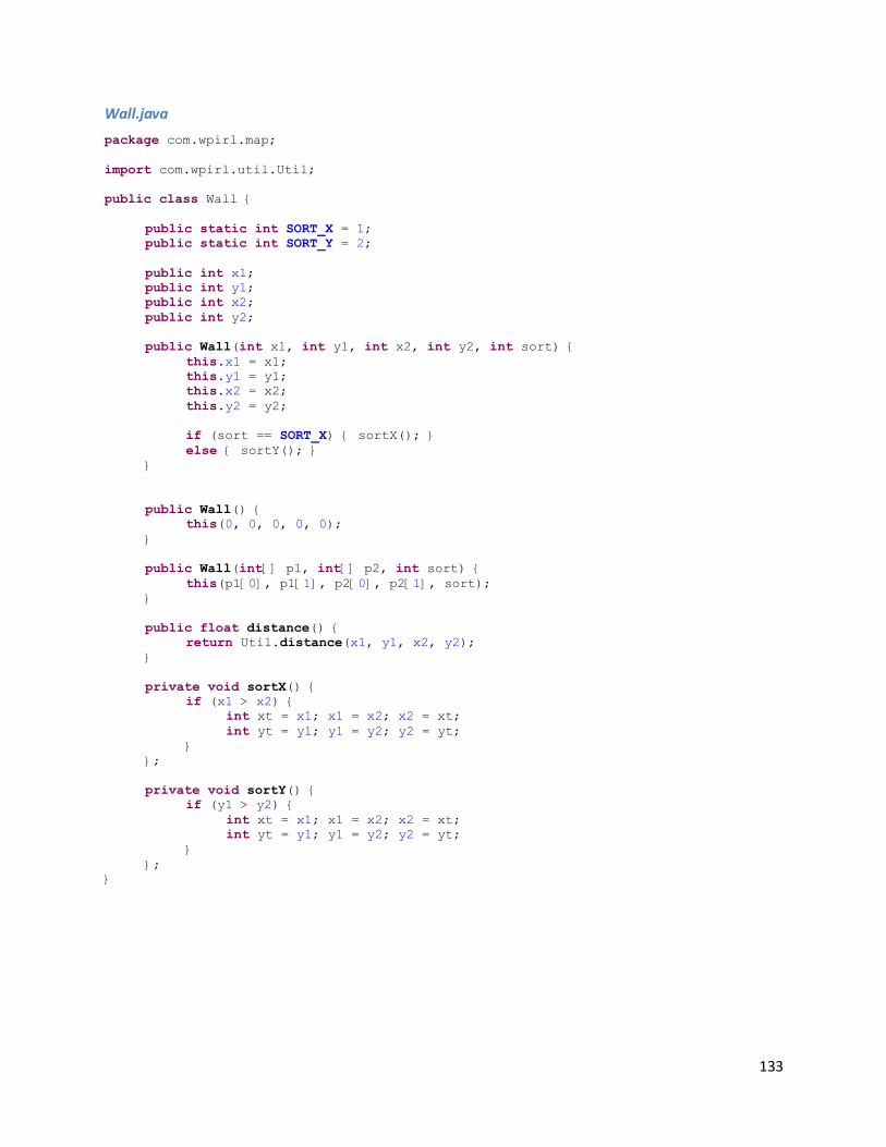
133
Wall.java
package com.wpirl.map;
import com.wpirl.util.Util;
public class Wall {
public static int SORT_X = 1;
public static int SORT_Y = 2;
public int x1;
public int y1;
public int x2;
public int y2;
public Wall(int x1, int y1, int x2, int y2, int sort) {
this.x1 = x1;
this.y1 = y1;
this.x2 = x2;
this.y2 = y2;
if (sort == SORT_X) { sortX(); }
else { sortY(); }
}
public Wall() {
this(0, 0, 0, 0, 0);
}
public Wall(int[] p1, int[] p2, int sort) {
this(p1[0], p1[1], p2[0], p2[1], sort);
}
public float distance() {
return Util.distance(x1, y1, x2, y2);
}
private void sortX() {
if (x1 > x2) {
int xt = x1; x1 = x2; x2 = xt;
int yt = y1; y1 = y2; y2 = yt;
}
};
private void sortY() {
if (y1 > y2) {
int xt = x1; x1 = x2; x2 = xt;
int yt = y1; y1 = y2; y2 = yt;
}
};
}
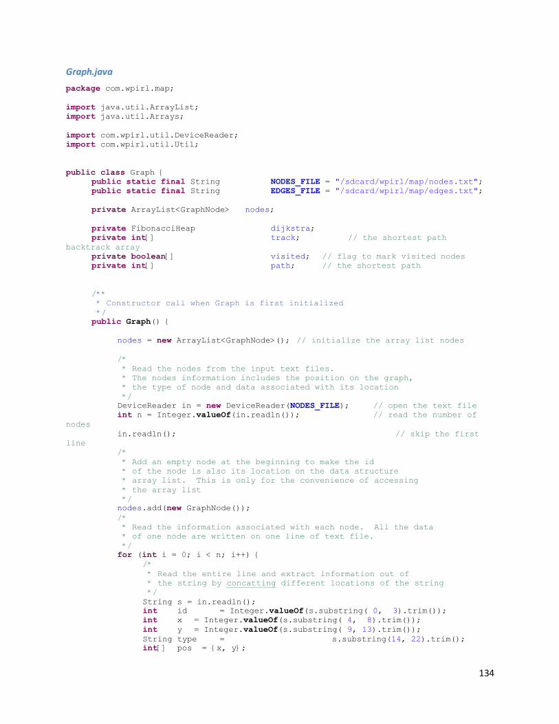
134
Graph.java
package com.wpirl.map;
import java.util.ArrayList;
import java.util.Arrays;
import com.wpirl.util.DeviceReader;
import com.wpirl.util.Util;
public class Graph {
public static final String NODES_FILE = "/sdcard/wpirl/map/nodes.txt";
public static final String EDGES_FILE = "/sdcard/wpirl/map/edges.txt";
private ArrayList<GraphNode> nodes;
private FibonacciHeap dijkstra;
private int[] track; // the shortest path
backtrack array
private boolean[] visited; // flag to mark visited nodes
private int[] path; // the shortest path
/**
* Constructor call when Graph is first initialized
*/
public Graph() {
nodes = new ArrayList<GraphNode>(); // initialize the array list nodes
/*
* Read the nodes from the input text files.
* The nodes information includes the position on the graph,
* the type of node and data associated with its location
*/
DeviceReader in = new DeviceReader(NODES_FILE); // open the text file
int n = Integer.valueOf(in.readln()); // read the number of
nodes
in.readln(); // skip the first
line
/*
* Add an empty node at the beginning to make the id
* of the node is also its location on the data structure
* array list. This is only for the convenience of accessing
* the array list
*/
nodes.add(new GraphNode());
/*
* Read the information associated with each node. All the data
* of one node are written on one line of text file.
*/
for (int i = 0; i < n; i++) {
/*
* Read the entire line and extract information out of
* the string by concatting different locations of the string
*/
String s = in.readln();
int id = Integer.valueOf(s.substring( 0, 3).trim());
int x = Integer.valueOf(s.substring( 4, 8).trim());
int y = Integer.valueOf(s.substring( 9, 13).trim());
String type = s.substring(14, 22).trim();
int[] pos = {x, y};
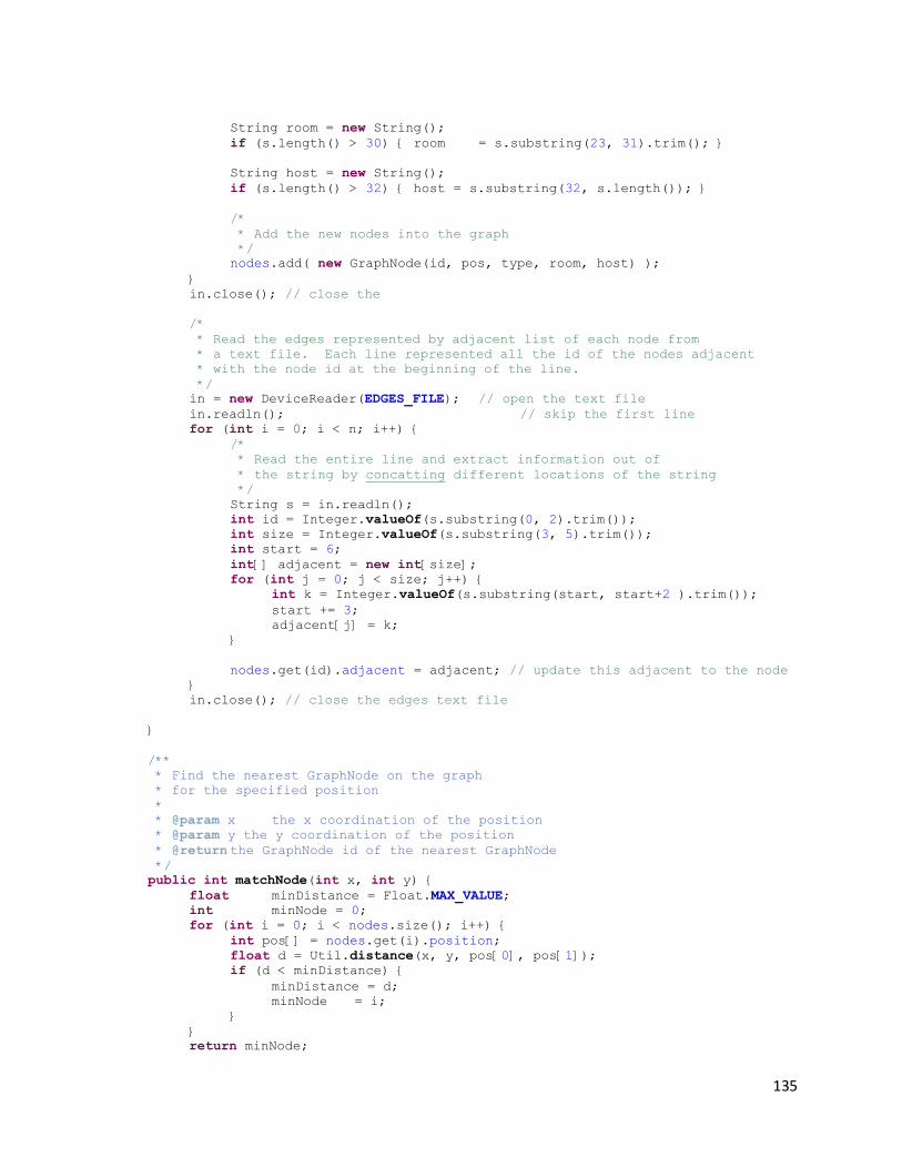
135
String room = new String();
if (s.length() > 30) { room = s.substring(23, 31).trim(); }
String host = new String();
if (s.length() > 32) { host = s.substring(32, s.length()); }
/*
* Add the new nodes into the graph
*/
nodes.add( new GraphNode(id, pos, type, room, host) );
}
in.close(); // close the
/*
* Read the edges represented by adjacent list of each node from
* a text file. Each line represented all the id of the nodes adjacent
* with the node id at the beginning of the line.
*/
in = new DeviceReader(EDGES_FILE); // open the text file
in.readln(); // skip the first line
for (int i = 0; i < n; i++) {
/*
* Read the entire line and extract information out of
* the string by concatting different locations of the string
*/
String s = in.readln();
int id = Integer.valueOf(s.substring(0, 2).trim());
int size = Integer.valueOf(s.substring(3, 5).trim());
int start = 6;
int[] adjacent = new int[size];
for (int j = 0; j < size; j++) {
int k = Integer.valueOf(s.substring(start, start+2 ).trim());
start += 3;
adjacent[j] = k;
}
nodes.get(id).adjacent = adjacent; // update this adjacent to the node
}
in.close(); // close the edges text file
}
/**
* Find the nearest GraphNode on the graph
* for the specified position
*
* @param x the x coordination of the position
* @param y the y coordination of the position
* @return the GraphNode id of the nearest GraphNode
*/
public int matchNode(int x, int y) {
float minDistance = Float.MAX_VALUE;
int minNode = 0;
for (int i = 0; i < nodes.size(); i++) {
int pos[] = nodes.get(i).position;
float d = Util.distance(x, y, pos[0], pos[1]);
if (d < minDistance) {
minDistance = d;
minNode = i;
}
}
return minNode;
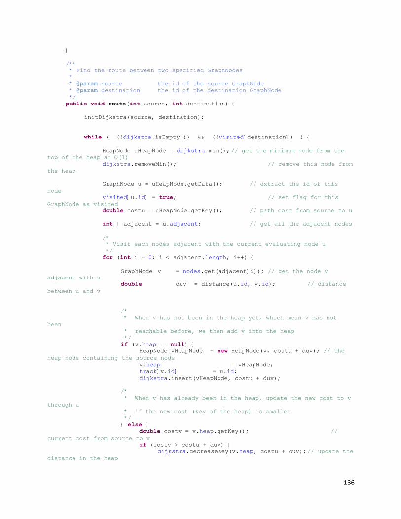
136
}
/**
* Find the route between two specified GraphNodes
*
* @param source the id of the source GraphNode
* @param destination the id of the destination GraphNode
*/
public void route(int source, int destination) {
initDijkstra(source, destination);
while ( (!dijkstra.isEmpty()) && (!visited[destination]) ) {
HeapNode uHeapNode = dijkstra.min(); // get the minimum node from the
top of the heap at O(1)
dijkstra.removeMin(); // remove this node from
the heap
GraphNode u = uHeapNode.getData(); // extract the id of this
node
visited[u.id] = true; // set flag for this
GraphNode as visited
double costu = uHeapNode.getKey(); // path cost from source to u
int[] adjacent = u.adjacent; // get all the adjacent nodes
/*
* Visit each nodes adjacent with the current evaluating node u
*/
for (int i = 0; i < adjacent.length; i++) {
GraphNode v = nodes.get(adjacent[i]); // get the node v
adjacent with u
double duv = distance(u.id, v.id); // distance
between u and v
/*
* When v has not been in the heap yet, which mean v has not
been
* reachable before, we then add v into the heap
*/
if (v.heap == null) {
HeapNode vHeapNode = new HeapNode(v, costu + duv); // the
heap node containing the source node
v.heap = vHeapNode;
track[v.id] = u.id;
dijkstra.insert(vHeapNode, costu + duv);
/*
* When v has already been in the heap, update the new cost to v
through u
* if the new cost (key of the heap) is smaller
*/
} else {
double costv = v.heap.getKey(); //
current cost from source to v
if (costv > costu + duv) {
dijkstra.decreaseKey(v.heap, costu + duv); // update the
distance in the heap
137
track[v.id] = u.id;
// update the track
}
}
}
} // dijkstra loop
track(source, destination);
}
/**
* initialize values used in dijkstra algorithm
*
* @param source id of the source GraphNode
* @param destination id of the destination GraphNode
*/
private void initDijkstra(int source, int destination) {
int size = nodes.size();
dijkstra = new FibonacciHeap();
track = new int[size];
visited = new boolean[size];
Arrays.fill(track, 0); // clear the track array
Arrays.fill(visited, false); // make the visited set empty
// clear the old heap reference in the nodes list
for (int i = 0; i < nodes.size(); i++) {
nodes.get(i).heap = null;
}
/*
* Set the source GraphNode dijkstra value = 0
* and put the source GraphNode at the top of the heap
*/
GraphNode sGraphNode = nodes.get(source); // the source node
in the graph
HeapNode sHeapNode = new HeapNode(sGraphNode, 0); // the heap node
containing the source node
sGraphNode.heap = sHeapNode; // put a
reference of the heap node pointer
dijkstra.insert(sHeapNode, 0);
}
/**
* Create the path found by the algorithm from source
* to destination using the track array recorded
*
* @param source the id of the source node
* @param destination the id of the destination node
*/
private void track(int source, int destination) {
int[] temp = new int[nodes.size()];
int count = 0;
int now = destination;
/*
* Get the path of the shortest route using the track array
* by tracing reversely from the destination back to the source
*/
while (now != 0) {
temp[count] = now;
now = track[now];
138
count++;
}
/*
* Reverse the path array to make the path go from source
* to destination.
*/
path = new int[count];
for (int i = 0; i < count; i++) {
path[i] = temp[count-i-1];
}
}
/**
* Return the distance between two GraphNodes by id
*
* @param source the id of the source node
* @param destination the id of the destination node
* @return the distance between the two nodes
*/
private float distance(int source, int destination) {
int[] s = nodes.get(source).position;
int[] d = nodes.get(destination).position;
return Util.distance(s, d);
}
/*
* ============================================================================
* get & set methods
* ============================================================================
*/
public ArrayList<GraphNode> getGraph() {
return nodes;
}
public int[] getPath() {
return path;
}
}
139
GraphNode.java
package com.wpirl.map;
import com.wpirl.util.Util;
public class GraphNode {
public static final int TYPE_CORRIDOR = 1;
public static final int TYPE_STAIR = 2;
public static final int TYPE_ELEVATOR = 3;
public static final int TYPE_ROOM = 4;
public int id;
public int[] position; // x y coordination (unit in pixels)
public int[] adjacent;
public int type;
public String room;
public String person;
public HeapNode heap;
public GraphNode(int id, int[] position, String type, String room, String person)
{
this.id = id;
this.position = new int[2];
this.position[0] = position[0];
this.position[1] = position[1];
this.room = room;
this.person = person;
if (type.compareToIgnoreCase("room" ) == 0) {
this.type = TYPE_ROOM;
} else if (type.compareToIgnoreCase("elevator") == 0) {
this.type = TYPE_ELEVATOR;
} else if (type.compareToIgnoreCase("stair" ) == 0) {
this.type = TYPE_STAIR;
} else if (type.compareToIgnoreCase("corridor") == 0) {
this.type = TYPE_CORRIDOR;
}
}
public GraphNode(int id, int x, int y) {
this.id = id;
this.position = new int[2];
this.position[0] = x;
this.position[1] = y;
}
public GraphNode(GraphNode node) {
this.id = node.id;
this.position = Util.copyArray(node.position);
this.adjacent = Util.copyArray(node.adjacent);
this.type = node.type;
this.room = node.room;
this.person = node.person;
}
public GraphNode() {
this.position = new int[2];
this.room = new String();

140
this.person = new String();
this.adjacent = new int[1];
}
}
141
FibonacciHeap.java
package com.wpirl.map;
import java.util.ArrayList;
import java.util.List;
import java.util.Stack;
/**
* This class implements a Fibonacci heap data structure used for Dijkstra algorithm
*
* The amortized running time of most of these methods is O(1).
* Several have an actual running time of O(1).
*
* removeMin() and delete() have O(log n) amortized running times because they do the
heap consolidation.
*/
public class FibonacciHeap {
private static final double oneOverLogPhi =
1.0 / Math.log((1.0 + Math.sqrt(5.0)) / 2.0);
private HeapNode minNode; // pointer to the minimum node in the heap
private int nNodes; // number of node in the heap
/**
* Constructs a FibonacciHeap object that contains no elements.
*/
public FibonacciHeap() {
} // DijkstraHeap()
/**
* Tests if the Fibonacci heap is empty or not. Returns true if the heap is
* empty, false otherwise.
*
* @return true if the heap is empty, false otherwise
*/
public boolean isEmpty() {
return minNode == null;
} // isEmpty
/**
* Removes all elements from this heap.
*/
public void clear() {
minNode = null;
nNodes = 0;
} // clear
/**
* Decreases the key value for a heap node, given the new value to take on.
* The structure of the heap may be changed and will not be consolidated.
*
* <p>Running time: O(1) amortized<p>
*
* @param x node to decrease the key of
* @param k new key value for node x
*
* @exception IllegalArgumentException Thrown if k is larger than x.key
* value.
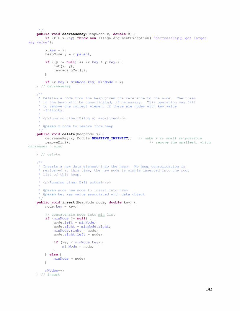
142
*/
public void decreaseKey(HeapNode x, double k) {
if (k > x.key) throw new IllegalArgumentException( "decreaseKey() got larger
key value");
x.key = k;
HeapNode y = x.parent;
if ((y != null) && (x.key < y.key)) {
cut(x, y);
cascadingCut(y);
}
if (x.key < minNode.key) minNode = x;
} // decreaseKey
/**
* Deletes a node from the heap given the reference to the node. The trees
* in the heap will be consolidated, if necessary. This operation may fail
* to remove the correct element if there are nodes with key value
* -Infinity.
*
* <p>Running time: O(log n) amortized</p>
*
* @param x node to remove from heap
*/
public void delete(HeapNode x) {
decreaseKey(x, Double.NEGATIVE_INFINITY); // make x as small as possible
removeMin(); // remove the smallest, which
decreases n also
} // delete
/**
* Inserts a new data element into the heap. No heap consolidation is
* performed at this time, the new node is simply inserted into the root
* list of this heap.
*
* <p>Running time: O(1) actual</p>
*
* @param node new node to insert into heap
* @param key key value associated with data object
*/
public void insert(HeapNode node, double key) {
node.key = key;
// concatenate node into min list
if (minNode != null) {
node.left = minNode;
node.right = minNode.right;
minNode.right = node;
node.right.left = node;
if (key < minNode.key) {
minNode = node;
}
} else {
minNode = node;
}
nNodes++;
} // insert
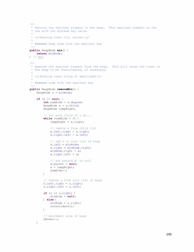
143
/**
* Returns the smallest element in the heap. This smallest element is the
* one with the minimum key value.
*
* <p>Running time: O(1) actual</p>
*
* @return heap node with the smallest key
*/
public HeapNode min() {
return minNode;
} // min
/**
* Removes the smallest element from the heap. This will cause the trees in
* the heap to be consolidated, if necessary.
*
* <p>Running time: O(log n) amortized</p>
*
* @return node with the smallest key
*/
public HeapNode removeMin() {
HeapNode z = minNode;
if (z != null) {
int numKids = z.degree;
HeapNode x = z.child;
HeapNode tempRight;
// for each child of z do...
while (numKids > 0) {
tempRight = x.right;
// remove x from child list
x.left.right = x.right;
x.right.left = x.left;
// add x to root list of heap
x.left = minNode;
x.right = minNode.right;
minNode.right = x;
x.right.left = x;
// set parent[x] to null
x.parent = null;
x = tempRight;
numKids--;
}
// remove z from root list of heap
z.left.right = z.right;
z.right.left = z.left;
if (z == z.right) {
minNode = null;
} else {
minNode = z.right;
consolidate();
}
// decrement size of heap
nNodes--;
}
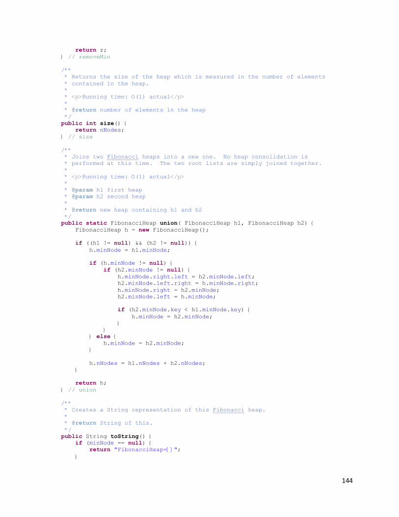
144
return z;
} // removeMin
/**
* Returns the size of the heap which is measured in the number of elements
* contained in the heap.
*
* <p>Running time: O(1) actual</p>
*
* @return number of elements in the heap
*/
public int size() {
return nNodes;
} // size
/**
* Joins two Fibonacci heaps into a new one. No heap consolidation is
* performed at this time. The two root lists are simply joined together.
*
* <p>Running time: O(1) actual</p>
*
* @param h1 first heap
* @param h2 second heap
*
* @return new heap containing h1 and h2
*/
public static FibonacciHeap union( FibonacciHeap h1, FibonacciHeap h2) {
FibonacciHeap h = new FibonacciHeap();
if ((h1 != null) && (h2 != null)) {
h.minNode = h1.minNode;
if (h.minNode != null) {
if (h2.minNode != null) {
h.minNode.right.left = h2.minNode.left;
h2.minNode.left.right = h.minNode.right;
h.minNode.right = h2.minNode;
h2.minNode.left = h.minNode;
if (h2.minNode.key < h1.minNode.key) {
h.minNode = h2.minNode;
}
}
} else {
h.minNode = h2.minNode;
}
h.nNodes = h1.nNodes + h2.nNodes;
}
return h;
} // union
/**
* Creates a String representation of this Fibonacci heap.
*
* @return String of this.
*/
public String toString() {
if (minNode == null) {
return "FibonacciHeap=[]";
}
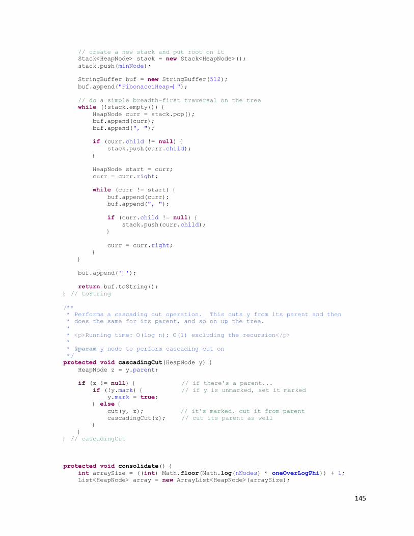
145
// create a new stack and put root on it
Stack<HeapNode> stack = new Stack<HeapNode>();
stack.push(minNode);
StringBuffer buf = new StringBuffer(512);
buf.append("FibonacciHeap=[");
// do a simple breadth-first traversal on the tree
while (!stack.empty()) {
HeapNode curr = stack.pop();
buf.append(curr);
buf.append(", ");
if (curr.child != null) {
stack.push(curr.child);
}
HeapNode start = curr;
curr = curr.right;
while (curr != start) {
buf.append(curr);
buf.append(", ");
if (curr.child != null) {
stack.push(curr.child);
}
curr = curr.right;
}
}
buf.append(']');
return buf.toString();
} // toString
/**
* Performs a cascading cut operation. This cuts y from its parent and then
* does the same for its parent, and so on up the tree.
*
* <p>Running time: O(log n); O(1) excluding the recursion</p>
*
* @param y node to perform cascading cut on
*/
protected void cascadingCut(HeapNode y) {
HeapNode z = y.parent;
if (z != null) { // if there's a parent...
if (!y.mark) { // if y is unmarked, set it marked
y.mark = true;
} else {
cut(y, z); // it's marked, cut it from parent
cascadingCut(z); // cut its parent as well
}
}
} // cascadingCut
protected void consolidate() {
int arraySize = ((int) Math.floor(Math.log(nNodes) * oneOverLogPhi)) + 1;
List<HeapNode> array = new ArrayList<HeapNode>(arraySize);
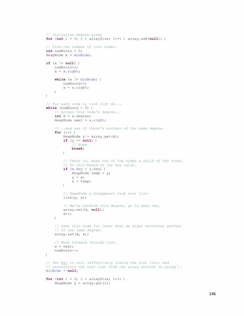
146
// Initialize degree array
for (int i = 0; i < arraySize; i++) { array.add(null); }
// Find the number of root nodes.
int numRoots = 0;
HeapNode x = minNode;
if (x != null) {
numRoots++;
x = x.right;
while (x != minNode) {
numRoots++;
x = x.right;
}
}
// For each node in root list do...
while (numRoots > 0) {
// Access this node's degree..
int d = x.degree;
HeapNode next = x.right;
// ..and see if there's another of the same degree.
for (;;) {
HeapNode y = array.get(d);
if (y == null) {
// Nope.
break;
}
// There is, make one of the nodes a child of the other.
// Do this based on the key value.
if (x.key > y.key) {
HeapNode temp = y;
y = x;
x = temp;
}
// HeapNode y disappears from root list.
link(y, x);
// We've handled this degree, go to next one.
array.set(d, null);
d++;
}
// Save this node for later when we might encounter another
// of the same degree.
array.set(d, x);
// Move forward through list.
x = next;
numRoots--;
}
// Set min to null (effectively losing the root list) and
// reconstruct the root list from the array entries in array[].
minNode = null;
for (int i = 0; i < arraySize; i++) {
HeapNode y = array.get(i);
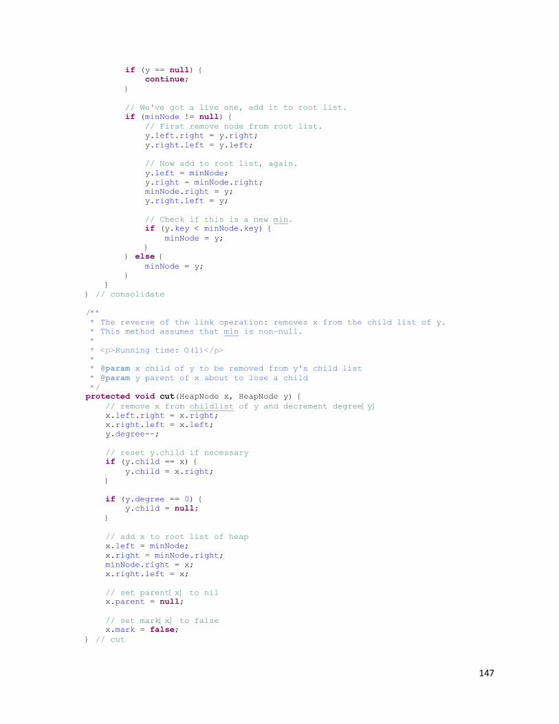
147
if (y == null) {
continue;
}
// We've got a live one, add it to root list.
if (minNode != null) {
// First remove node from root list.
y.left.right = y.right;
y.right.left = y.left;
// Now add to root list, again.
y.left = minNode;
y.right = minNode.right;
minNode.right = y;
y.right.left = y;
// Check if this is a new min.
if (y.key < minNode.key) {
minNode = y;
}
} else {
minNode = y;
}
}
} // consolidate
/**
* The reverse of the link operation: removes x from the child list of y.
* This method assumes that min is non-null.
*
* <p>Running time: O(1)</p>
*
* @param x child of y to be removed from y's child list
* @param y parent of x about to lose a child
*/
protected void cut(HeapNode x, HeapNode y) {
// remove x from childlist of y and decrement degree[y]
x.left.right = x.right;
x.right.left = x.left;
y.degree--;
// reset y.child if necessary
if (y.child == x) {
y.child = x.right;
}
if (y.degree == 0) {
y.child = null;
}
// add x to root list of heap
x.left = minNode;
x.right = minNode.right;
minNode.right = x;
x.right.left = x;
// set parent[x] to nil
x.parent = null;
// set mark[x] to false
x.mark = false;
} // cut
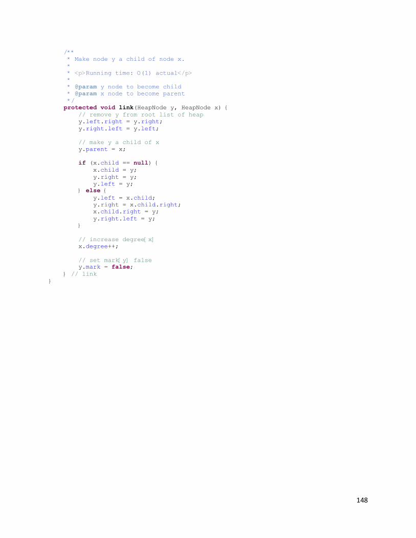
148
/**
* Make node y a child of node x.
*
* <p>Running time: O(1) actual</p>
*
* @param y node to become child
* @param x node to become parent
*/
protected void link(HeapNode y, HeapNode x) {
// remove y from root list of heap
y.left.right = y.right;
y.right.left = y.left;
// make y a child of x
y.parent = x;
if (x.child == null) {
x.child = y;
y.right = y;
y.left = y;
} else {
y.left = x.child;
y.right = x.child.right;
x.child.right = y;
y.right.left = y;
}
// increase degree[x]
x.degree++;
// set mark[y] false
y.mark = false;
} // link
}
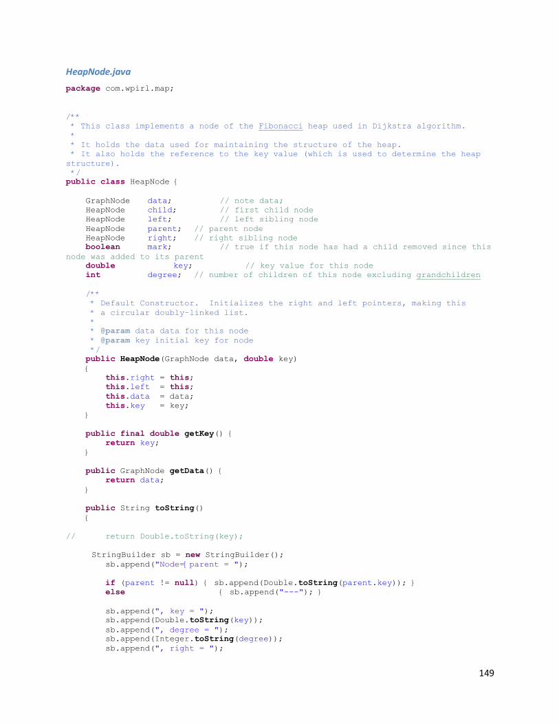
149
HeapNode.java
package com.wpirl.map;
/**
* This class implements a node of the Fibonacci heap used in Dijkstra algorithm.
*
* It holds the data used for maintaining the structure of the heap.
* It also holds the reference to the key value (which is used to determine the heap
structure).
*/
public class HeapNode {
GraphNode data; // note data;
HeapNode child; // first child node
HeapNode left; // left sibling node
HeapNode parent; // parent node
HeapNode right; // right sibling node
boolean mark; // true if this node has had a child removed since this
node was added to its parent
double key; // key value for this node
int degree; // number of children of this node excluding grandchildren
/**
* Default Constructor. Initializes the right and left pointers, making this
* a circular doubly-linked list.
*
* @param data data for this node
* @param key initial key for node
*/
public HeapNode(GraphNode data, double key)
{
this.right = this;
this.left = this;
this.data = data;
this.key = key;
}
public final double getKey() {
return key;
}
public GraphNode getData() {
return data;
}
public String toString()
{
// return Double.toString(key);
StringBuilder sb = new StringBuilder();
sb.append("Node=[parent = ");
if (parent != null) { sb.append(Double.toString(parent.key)); }
else { sb.append("---"); }
sb.append(", key = ");
sb.append(Double.toString(key));
sb.append(", degree = ");
sb.append(Integer.toString(degree));
sb.append(", right = ");
150
if (right != null) { sb.append(Double.toString(right.key)); }
else { sb.append("---"); }
sb.append(", left = ");
if (left != null) { sb.append(Double.toString(left.key)); }
else { sb.append("---"); }
sb.append(", child = ");
if (child != null) { sb.append(Double.toString(child.key)); }
else { sb.append("---"); }
sb.append(']');
return sb.toString();
}
}
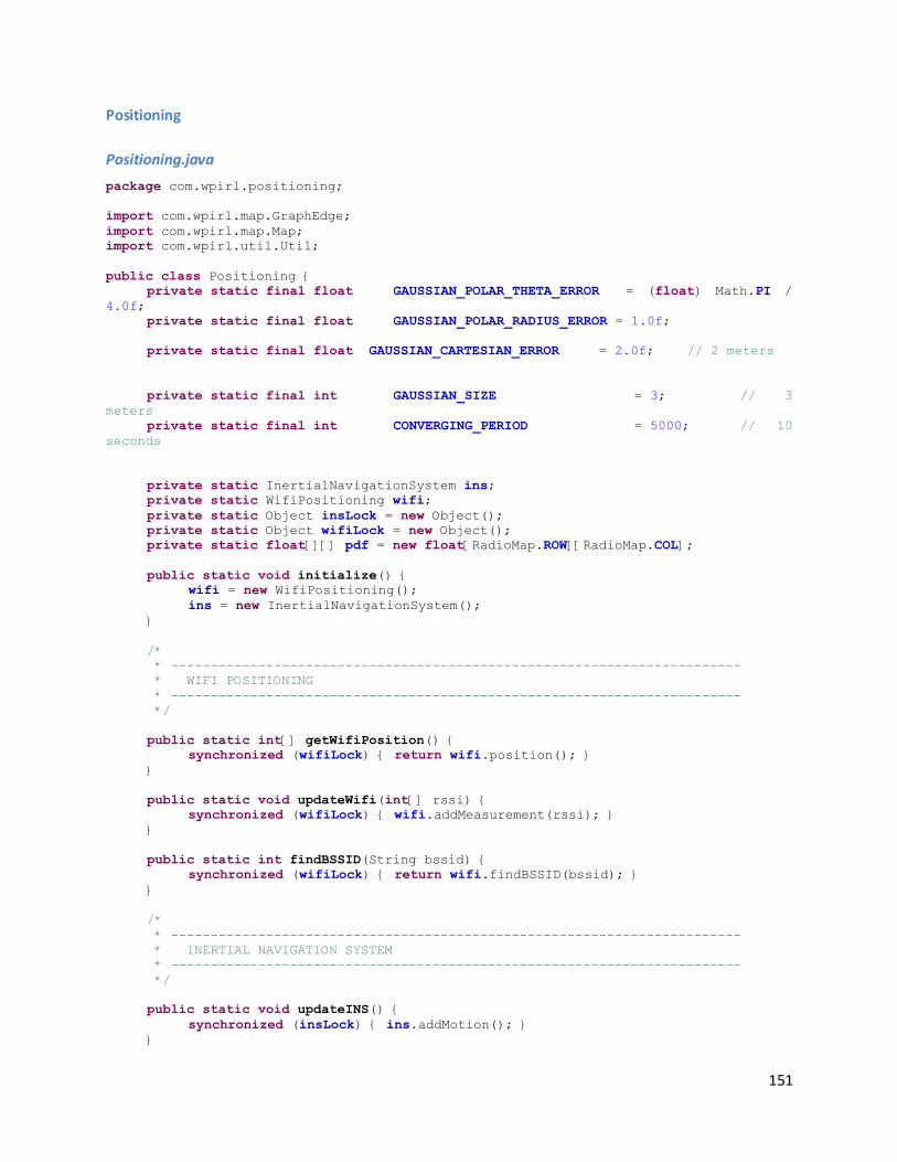
151
Positioning
Positioning.java
package com.wpirl.positioning;
import com.wpirl.map.GraphEdge;
import com.wpirl.map.Map;
import com.wpirl.util.Util;
public class Positioning {
private static final float GAUSSIAN_POLAR_THETA_ERROR = (float) Math.PI /
4.0f;
private static final float GAUSSIAN_POLAR_RADIUS_ERROR = 1.0f;
private static final float GAUSSIAN_CARTESIAN_ERROR = 2.0f; // 2 meters
private static final int GAUSSIAN_SIZE = 3; // 3
meters
private static final int CONVERGING_PERIOD = 5000; // 10
seconds
private static InertialNavigationSystem ins;
private static WifiPositioning wifi;
private static Object insLock = new Object();
private static Object wifiLock = new Object();
private static float[][] pdf = new float[RadioMap.ROW][RadioMap.COL];
public static void initialize() {
wifi = new WifiPositioning();
ins = new InertialNavigationSystem();
}
/*
* ------------------------------------------------------------------------
* WIFI POSITIONING
* ------------------------------------------------------------------------
*/
public static int[] getWifiPosition() {
synchronized (wifiLock) { return wifi.position(); }
}
public static void updateWifi(int[] rssi) {
synchronized (wifiLock) { wifi.addMeasurement(rssi); }
}
public static int findBSSID(String bssid) {
synchronized (wifiLock) { return wifi.findBSSID(bssid); }
}
/*
* ------------------------------------------------------------------------
* INERTIAL NAVIGATION SYSTEM
* ------------------------------------------------------------------------
*/
public static void updateINS() {
synchronized (insLock) { ins.addMotion(); }
}
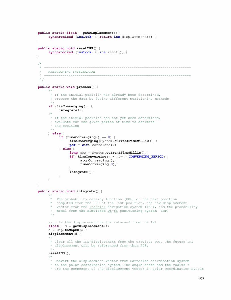
152
public static float[] getDisplacement() {
synchronized (insLock) { return ins.displacement(); }
}
public static void resetINS() {
synchronized (insLock) { ins.reset(); }
}
/*
* ------------------------------------------------------------------------
* POSITIONING INTEGRATION
* ------------------------------------------------------------------------
*/
public static void process() {
/*
* If the initial position has already been determined,
* process the data by fusing different positioning methods
*/
if (!isConverging()) {
integrate();
/*
* If the initial position has not yet been determined,
* evaluate for the given period of time to estimate
* the position
*/
} else {
if (timeConverging() == 0) {
timeConverging(System.currentTimeMillis());
pdf = wifi.correlate();
} else {
long now = System.currentTimeMillis();
if (timeConverging() - now > CONVERGING_PERIOD) {
stopConverging();
timeConverging(0);
}
integrate();
}
}
}
public static void integrate() {
/*
* The probability density function (PDF) of the next position
* computed from the PDF of the last position, the new displacement
* vector from the inertial navigation system (INS), and the probability
* model from the simulated wi-fi positioning system (SWP)
*/
// d is the displacement vector returned from the INS
float[] d = getDisplacement();
d = Map.toMapCS(d);
displacement(d);
/*
* Clear all the INS displacement from the previous PDF. The future INS
* displacement will be referenced from this PDF.
*/
resetINS();
/*
* Convert the displacement vector from Cartesian coordination system
* to the polar coordination system. The angle theta and the radius r
* are the component of the displacement vector in polar coordination system
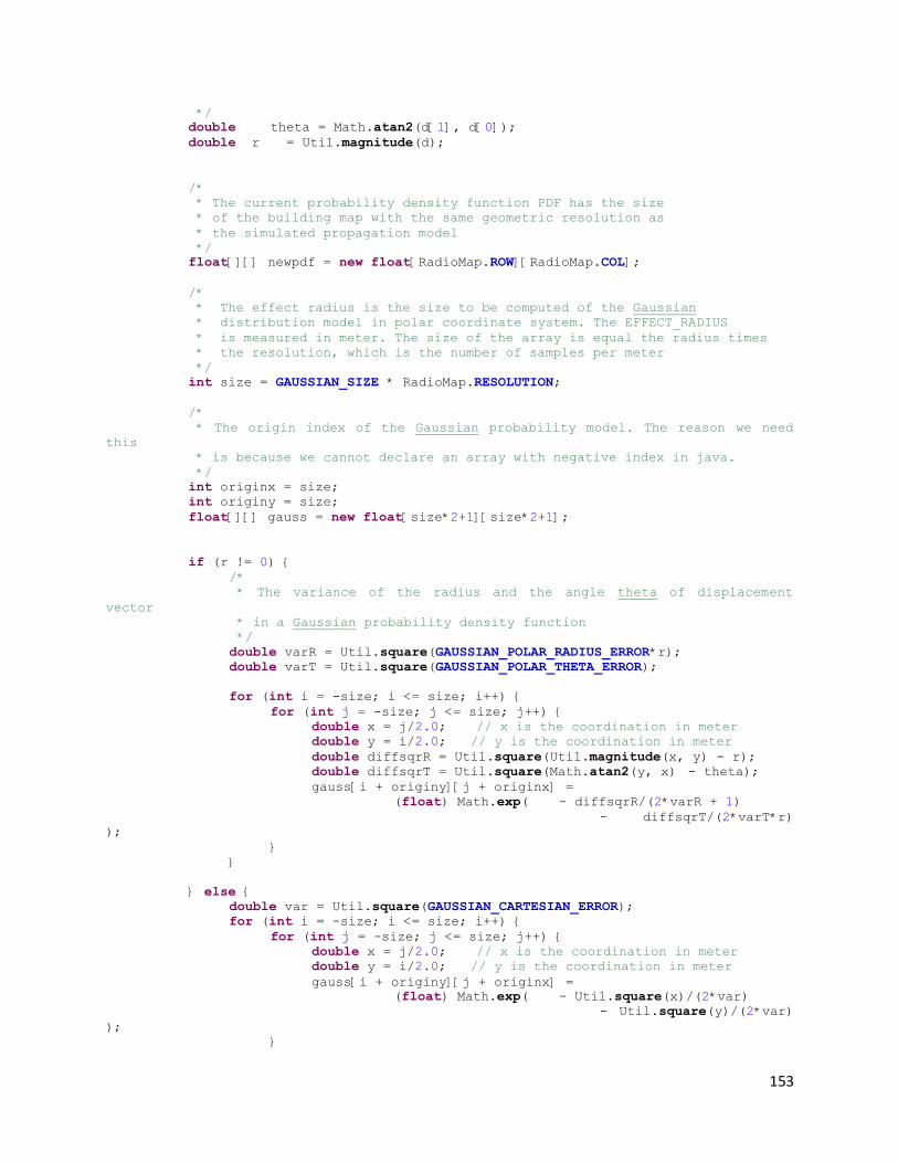
153
*/
double theta = Math.atan2(d[1], d[0]);
double r = Util.magnitude(d);
/*
* The current probability density function PDF has the size
* of the building map with the same geometric resolution as
* the simulated propagation model
*/
float[][] newpdf = new float[RadioMap.ROW][RadioMap.COL];
/*
* The effect radius is the size to be computed of the Gaussian
* distribution model in polar coordinate system. The EFFECT_RADIUS
* is measured in meter. The size of the array is equal the radius times
* the resolution, which is the number of samples per meter
*/
int size = GAUSSIAN_SIZE * RadioMap.RESOLUTION;
/*
* The origin index of the Gaussian probability model. The reason we need
this
* is because we cannot declare an array with negative index in java.
*/
int originx = size;
int originy = size;
float[][] gauss = new float[size*2+1][size*2+1];
if (r != 0) {
/*
* The variance of the radius and the angle theta of displacement
vector
* in a Gaussian probability density function
*/
double varR = Util.square(GAUSSIAN_POLAR_RADIUS_ERROR*r);
double varT = Util.square(GAUSSIAN_POLAR_THETA_ERROR);
for (int i = -size; i <= size; i++) {
for (int j = -size; j <= size; j++) {
double x = j/2.0; // x is the coordination in meter
double y = i/2.0; // y is the coordination in meter
double diffsqrR = Util.square(Util.magnitude(x, y) - r);
double diffsqrT = Util.square(Math.atan2(y, x) - theta);
gauss[i + originy][j + originx] =
(float) Math.exp( - diffsqrR/(2*varR + 1)
- diffsqrT/(2*varT*r)
);
}
}
} else {
double var = Util.square(GAUSSIAN_CARTESIAN_ERROR);
for (int i = -size; i <= size; i++) {
for (int j = -size; j <= size; j++) {
double x = j/2.0; // x is the coordination in meter
double y = i/2.0; // y is the coordination in meter
gauss[i + originy][j + originx] =
(float) Math.exp( - Util.square(x)/(2*var)
- Util.square(y)/(2*var)
);
}
154
}
}
float[][] wp = wifi.correlate();
float max = Float.MIN_VALUE;
int[] maxpos = new int[2];
for (int i = 0; i < RadioMap.ROW; i++) {
for (int j = 0; j < RadioMap.COL; j++) {
newpdf[i][j] = 0;
/*
* The previous PDF is used as the confident of the last position
* With the gaussian distribution from the displacement vector,
* using the probability from the last PDF as a weight, we then
sum
* all these gaussian accross the entire old PDF to get new PDF.
*/
for (int ig = -size; ig <= size; ig++) {
for (int jg = -size; jg <= size; jg++) {
if ((i + ig >= 0) && (i + ig < RadioMap.ROW)) {
if ((j + jg >= 0) && (j + jg < RadioMap.COL)) {
newpdf[i][j] += pdf[i + ig][j + jg] *
gauss[originy - ig][originx -
jg];
}
}
}
}
/*
* Correlate the PDF with the wifi positioning system PDF
*/
newpdf[i][j] *= wp[i][j];
if (newpdf[i][j] > max) {
max = newpdf[i][j];
maxpos[0] = j;
maxpos[1] = i;
}
}
}
for (int i = 0; i < RadioMap.ROW; i++) {
for (int j = 0; j < RadioMap.COL; j++) {
newpdf[i][j] /= max;
}
}
pdf = newpdf;
float[] pos = RadioMap.toActualScale(maxpos);
position(pos);
int[] mappos = Map.toMapScale(pos);
mappos = Util.translate(mappos, -RadioMap.LEFT, -RadioMap.TOP);
Map.match(mappos[0], mappos[1]);
}
/*
* ------------------------------------------------------------------------
* CONVERGEANCE
* ------------------------------------------------------------------------
*/
155
private static boolean isConverging;
private static Object isConvergingLock = new Object();
public static void startConverging() {
synchronized (isConvergingLock) { isConverging = true; }
}
public static void stopConverging() {
synchronized (isConvergingLock) { isConverging = false; }
}
public static boolean isConverging() {
synchronized (isConvergingLock) { return isConverging; }
}
private static long timeConverging;
private static Object timeConvergingLock = new Object();
public static void timeConverging(long time) {
synchronized (timeConvergingLock) { timeConverging = time; }
}
public static long timeConverging() {
synchronized (timeConvergingLock) { return timeConverging; }
}
/*
* ------------------------------------------------------------------------
* SYNCHRONIZED POSITION
* ------------------------------------------------------------------------
*/
private static float[] position = new float[2];
private static Object positionLock = new Object();
public static void position(float[] p) {
synchronized (positionLock) { Util.copyArray(position, p); }
}
public static float[] position() {
synchronized (positionLock) { return Util.copyArray(position); }
}
private static float[] displacement = new float[2];
private static Object displacementLock = new Object();
public static void displacement(float[] p) {
synchronized (displacementLock) { Util.copyArray(displacement, p); }
}
public static float[] displacement() {
synchronized (displacementLock) { return Util.copyArray(displacement); }
}
/*
* ------------------------------------------------------------------------
* SYNCHRONIZED RECORDING
* ------------------------------------------------------------------------
*/
private static boolean isRecording;
private static Object isRecordingLock = new Object();
public static void startRecording() {
synchronized (isRecordingLock) { isRecording = true; }
}
public static void stopRecording() {
156
synchronized (isRecordingLock) { isRecording = false; }
}
public static boolean isRecording() {
synchronized (isRecordingLock) { return isRecording; }
}
/*
* ------------------------------------------------------------------------
* SYNCHRONIZED POSITIONING
* ------------------------------------------------------------------------
*/
private static boolean isPositioning;
private static Object isPositioningLock = new Object();
public static void startPositioning() {
synchronized (isPositioningLock) { isPositioning = true; }
}
public static void stopPositioning() {
synchronized (isPositioningLock) { isPositioning = false; }
}
public static boolean isPositioning() {
synchronized (isPositioningLock) { return isPositioning; }
}
/*
* ------------------------------------------------------------------------
* MAP MATCHING
* ------------------------------------------------------------------------
*/
private static int[] matchedPoint = new int[2];
private static Object matchedPointLock = new Object();
public static void matchedPoint(int[] point) {
synchronized (matchedPointLock) { Util.copyArray(matchedPoint, point); }
}
public static int[] matchedPoint() {
synchronized (matchedPointLock) { return Util.copyArray(matchedPoint); }
}
private static GraphEdge matchedEdge = new GraphEdge();
private static Object matchedEdgeLock = new Object();
public static void matchedEdge(GraphEdge edge) {
synchronized (matchedEdgeLock) { matchedEdge = new GraphEdge(edge); }
}
public static GraphEdge matchedEdge() {
synchronized (matchedEdgeLock) { return new GraphEdge(matchedEdge); }
}
}
157
DeviceSensor.java
package com.wpirl.positioning;
import android.hardware.SensorManager;
import com.wpirl.util.Util;
public class DeviceSensor {
private static final float MOVEMENT = 0.5f;
private static final int WINDOW_SUMMATION_SIZE = 30; // 50 * 20 ms = 1
second
private static final float EARTH_GRAVITY =
SensorManager.GRAVITY_EARTH; // 9.80755f
private static final float EARTH_GEOMAGNETIC = 47.0f;
private static final float THRESHOLD_GRAVITY = 1.0f;
private static final float THRESHOLD_GEOMAGNETIC = 3.0f;
public static Object lockSensing = new Object();
public static float[] devA = new float[3];
public static float[] devM = new float[3];
public static float[] devO = new float[3];
public static float[] gravity = new float[3];
public static float[] geomagnetic = new float[3];
public static float[] refA = new float[3];
public static float[] refO = new float[3];
public static float[] mR = new float[9];
public static float[] mI = new float[9];
public static Object lockMoving = new Object();
public static boolean flagMoving = false;
public static int wsPosition = 0;
public static float wsAggregate = 0;
public static float[] wsSequence = new float[WINDOW_SUMMATION_SIZE];
/**
* Set the accelerometer sample values
* and calibrate the data if required
*
* * @param raw The raw output from accelerometer
*/
public static void setDevA(float[] raw) {
synchronized (lockSensing) {
Util.copyArray(devA, raw);
/*
* Add new acceleration to the window summation
* sequences and find the variance to compare
*
* Note: the sequence is constructed as a rotation array with the
wsPosition
* is the position of the latest value
*/
aggregrateMotion();
float magnitude = Util.magnitude(devA);
float threshold = THRESHOLD_GRAVITY;
158
if (Math.abs(magnitude - EARTH_GRAVITY) <= threshold) {
Util.copyArray(gravity, devA);
}
}
}
/**
* Set the magnetic sample values
* and calibrate the data if required
*
* @param raw The raw magnetic output from sensor
*/
public static void setDevM(float[] raw) {
synchronized (lockSensing) {
Util.copyArray(devM, raw);
/*
* Update the geomagnetic vector if this sample
* under the threshold
*/
float magnitude = Util.magnitude(devM);
if (Math.abs(magnitude - EARTH_GEOMAGNETIC) <= THRESHOLD_GEOMAGNETIC) {
Util.copyArray(geomagnetic, devM);
}
}
}
public static void setDevO(float[] raw) {
synchronized (lockSensing) {
Util.copyArray(devO, raw);
}
}
/**
* Convert the sensor data from the device's coordination system
* to the world's coordination system including motion and orientation
*
* @return true if convertible
*/
public static boolean toEarthCS() {
synchronized (lockSensing) {
// When current gravity and current geomagnetic are known
if ((Util.magnitude(devA) > 0) && (Util.magnitude(devM) > 0)) {
/*
* compute the rotation matrix from the current gravity and
geomanetic
* the rotation matrix is used to transpose from the device's
coordination system
* to the world's coordination system
*/
SensorManager.getRotationMatrix(mR, mI, gravity, geomagnetic);
/*
* compute the orientation of the device from rotation matrix
* including azimuth, pitch and roll angles of the device's
current position
* in the world's coordination system
*/
SensorManager.getOrientation(mR, refO);
/*
159
* compute the acceleration in the world's coordination system
* by multiplying the device acceleration with the rotation
matrix
*
* | refA0 | | mR0 mR1 mR2 | | devA0 |
* | refA1 | = | mR3 mR4 mR5 | * | devA1 |
* | refA2 | | mR6 mR7 mR8 | | devA2 |
*/
refA[0] = devA[0] * mR[0] +
devA[1] * mR[1] +
devA[2] * mR[2];
refA[1] = devA[0] * mR[3] +
devA[1] * mR[4] +
devA[2] * mR[5];
refA[2] = devA[0] * mR[6] +
devA[1] * mR[7] +
devA[2] * mR[8];
return true;
} else {
return false;
}
}
}
/**
* Synchronized get function to get the reference acceleration
* in the Earth's coordination system
*
* @return the vector containing the acceleration in (x, y, z)
*/
public static float[] getRefAcceleration() {
float[] result = new float[3];
synchronized (lockSensing) {
Util.copyArray(result, refA);
}
return result;
}
/*
* ============================================================================
* Motion detection methods
* ============================================================================
*/
/**
* Return the angle between the device direction
* and the north direction in the Earth's coordination system
*
* @return the heading angle in degrees
*/
public static float getHeading() {
float degrees;
synchronized (lockSensing) {
degrees = (float) devO[0];
}
return degrees;
}
public static void enableMoving() {
160
synchronized (lockMoving) {
flagMoving = true;
}
}
public static void disableMoving() {
synchronized (lockMoving) {
flagMoving = false;
}
}
public static boolean isMoving() {
synchronized (lockMoving) {
if (flagMoving) return true;
else return false;
}
}
private static void aggregrateMotion() {
float magnitude = Util.magnitude(devA);
/*
* The wsSequence contains the last N samples output from
* the sensor. The sequence is implemented using a rotation array.
* The rotation array uses a fixed array and a rotation wsPosition
* to indicate the position of the next samples
*/
/*
* If this wsPosition is out of bound, go back to the
* beginning of the fixed array, thus make the rotation
*/
wsPosition++;
if (wsPosition == WINDOW_SUMMATION_SIZE) wsPosition = 0;
/*
* The wsAggregate is the sum of all the value in the rotation
* array. A new sum is computed by deducting old value and replace
* it with the new value.
*/
wsAggregate = wsAggregate - wsSequence[wsPosition] + magnitude;
wsSequence[wsPosition] = magnitude;
/*
* The length of the rotation array. This is not at maximum length
* only at the beginning of the sampling period when the program
* just launches and the number of samples has not reached the maximum N.
* After the first N samples, the length is always N.
*/
int length;
if (wsSequence[WINDOW_SUMMATION_SIZE - 1] == 0) {
length = wsPosition + 1;
} else {
length = WINDOW_SUMMATION_SIZE;
}
float mean = wsAggregate / length; // the arithmetic mean (average)
float stdev = 0; // the standard deviation
/*
161
* Compute the variance of the wsSequence
*/
for (int i = 0; i < length; i++) {
stdev += (wsSequence[i] - mean) * (wsSequence[i] - mean);
}
stdev = (float) Math.sqrt(stdev/length);
/*
* If the standard deviation is below the threshold
* the phone is not in motion.
*/
if (stdev > MOVEMENT) { enableMoving(); }
else { disableMoving(); }
}
}
162
InertialNavigationSystem.java
package com.wpirl.positioning;
import java.util.LinkedList;
import com.wpirl.util.Util;
public class InertialNavigationSystem {
public static final int MAX_SIZE = 1000;
public static final float HUMAN_SPEED_WALK = 5000.0f/3600.0f; //
5km/3600s
private LinkedList<Motion> motions;
public InertialNavigationSystem() {
motions = new LinkedList<Motion>();
}
public void reset() {
if (!motions.isEmpty()) motions.clear();
long time = System.currentTimeMillis();
motions.add(new Motion(time));
}
/**
* Add new motion sample to the queue
* @param a acceleration
* @param t time
*/
public void addMotion() {
// If the queue is full, remove the first element
if (motions.size() == MAX_SIZE) { motions.removeFirst(); }
long time = System.currentTimeMillis();
float dt = (time - motions.getLast().time)/1000.0f;
float[] d = Util.copyArray(motions.getLast().distance);
Motion current = new Motion(time);
if (DeviceSensor.isMoving()) {
// moved distance
float distance = HUMAN_SPEED_WALK * dt;
float heading = (float) Math.toRadians(DeviceSensor.getHeading());
current.distance[0] = d[0] + distance * (float) Math.sin(heading);
current.distance[1] = d[1] + distance * (float) Math.cos(heading);
} else {
current.distance[0] = d[0];
current.distance[1] = d[1];
}
// add the new motion element to the end of the queue
motions.addLast(current);
}
public float[] displacement() {
float[] d = Util.copyArray(motions.getLast().distance);
return d;
}
}
163
Motion.java
package com.wpirl.positioning;
import com.wpirl.util.Util;
public class Motion {
public float[] distance;
public long time;
public Motion() {
this.distance = new float[2];
this.time = 0;
}
public Motion(long time) {
this.distance = new float[2];
this.time = time;
}
public Motion(Motion m) {
this.distance = Util.copyArray(m.distance);
this.time = m.time;
}
}
164
WifiPositioning.java
package com.wpirl.positioning;
import com.wpirl.util.DeviceReader;
import com.wpirl.util.Util;
public class WifiPositioning {
public static final int WAP_NUMBER = 6; // 5 wireless access points
public static final int WAP_COUNT = 4;
public static final int VALUE_LENGTH = 8; // 6 digits + minus sign '-' +
decimal point '.'
public static final String SIMULATION_FILE =
"/sdcard/wpirl/simulation_model/WAP";
public static final int MAX_COUNT = 5;
private RadioMap[] simulation; // the router simulated map
private int[] rssi;
/**
* Read the simulated model from input file stored
* in the sdcard at location /sdcard/locus/simulation_model/
* with name format is WAP# with # is the order number
*/
public WifiPositioning() {
simulation = new RadioMap[WAP_NUMBER];
rssi = new int[WAP_NUMBER];
input();
}
private void input() {
// for each simulation file containing the radio map of one wireless access
point
for (int k = 0; k < WAP_NUMBER; k++) {
String file = new String(SIMULATION_FILE + String.valueOf(k+1) +
".txt"); // the path of the file
DeviceReader in = new DeviceReader(file);
// open the file to read
String s = in.readln();
// read the first line
s = s.toLowerCase();
simulation[k] = new RadioMap();
simulation[k].bssid = s;
// the first line is BSSID (MAC address)
s = in.readln();
// skip the next line
for (int i = 0; i < RadioMap.ROW; i++) {
// browse the number of row
s = in.readln();
// read the entire line
int start = 0;
int j = 0;
// start with column 0
/*
* Each value contains exact 8 characters:
* 6 digits, 1 minus sign '-', and 1 decimal point '.'
* The value will be read from position: 0, 8, 16, etc.
*/
165
while (j < RadioMap.COL) {
String value = s.substring(start, start + VALUE_LENGTH);
// the value at row i column j
start += VALUE_LENGTH;
simulation[k].map[i][j] = Float.valueOf(value);
// record the value
j++;
}
}
in.close();
}
}
/**
* Return the probability density function of the last sample
* based on the simulated propagation models
*
* @param rssi
* @return
*/
public float[][] correlate() {
float[][] c = new float[RadioMap.ROW][RadioMap.COL];
boolean[] highest = Util.highest(rssi, WAP_COUNT);
int[] maxpos = new int[2];
float max = 0;
for (int i = 0; i < RadioMap.ROW; i++) {
for (int j = 0; j < RadioMap.COL; j++) {
c[i][j] = 1;
for (int k = 0; k < WAP_NUMBER; k++) {
if ( (rssi[k] > Integer.MIN_VALUE) && (highest[k]) ) {
float square = Util.square(rssi[k] -
simulation[k].map[i][j]);
c[i][j] *= (double) Math.exp(( square ) / (5*rssi[k])
);
if (c[i][j] > max) {
max = c[i][j];
maxpos[0] = j;
maxpos[1] = i;
}
}
}
}
}
addPosition(maxpos);
return c;
}
public void addMeasurement(int[] rssi) {
Util.copyArray(this.rssi, rssi);
}
/**
* Find the id of the WAP in simulation maps using the
* BSSID (physical MAC address of the router). In the WAP
* is among the simulated propagation models, return the id of
* that WAP, else return -1 if this WAP is not in the model.
166
*
* @param bssid The BSSID of the WAP to search
* @return The id of the simulated model of this WAP
*/
public int findBSSID(String bssid) {
for (int k = 0; k < WAP_NUMBER; k++) {
if (bssid.equals(simulation[k].bssid)) {
return k;
};
}
return -1;
}
private int[][] position = new int[MAX_COUNT][2];
private double[] average = new double[2];
private int count = 0;
public void addPosition(int[] newpos) {
double[] d = new double[MAX_COUNT];
double sum = 0;
position[count][0] = newpos[0];
position[count][1] = newpos[1];
int length;
if (position[MAX_COUNT-1][0] + position[MAX_COUNT-1][1] == 0) {
length = count+1;
} else {
length = MAX_COUNT;
}
count++;
if (count == MAX_COUNT) count = 0;
if (length > 1) {
for (int i = 0; i < length; i++) {
d[i] = Util.distance(position[i][0], position[i][1], average[0],
average[1]);
sum += d[i];
}
average[0] = 0;
average[1] = 0;
for (int i = 0; i < length; i++) {
average[0] += ((double) position[i][0]) * (sum - d[i]) /
((length - 1) * sum);
average[1] += ((double) position[i][1]) * (sum - d[i]) /
((length - 1) * sum);
}
} else {
average[0] = position[0][0];
average[1] = position[0][1];
}
}
public int[] average() {
int[] value = new int[2];
value[0] = (int) average[0];
value[1] = (int) average[1];
return value;
}

167
public int[] position() {
int[] value = Util.copyArray(position[count]);
return value;
}
}
168
RadioMap.java
package com.wpirl.positioning;
public class RadioMap {
public static final int RESOLUTION = 2; // 2 sample per meter
public static final int LEFT = 74;
public static final int TOP = 188;
public static final int ROW = 94;
public static final int COL = 25;
public float[][] map;
public String bssid;
public RadioMap() {
map = new float[ROW][COL];
}
public String toString() {
StringBuilder sb = new StringBuilder();
for (int i = 0; i < ROW; i++) {
for (int j = 0; j < COL; j++) {
sb.append(String.valueOf(map[i][j]));
}
sb.append("\n");
}
return sb.toString();
}
}
169
View
MapView.java
package com.wpirl.view;
import java.util.ArrayList;
import android.content.Context;
import android.graphics.Bitmap;
import android.graphics.BitmapFactory;
import android.graphics.Canvas;
import android.graphics.Color;
import android.graphics.ComposePathEffect;
import android.graphics.CornerPathEffect;
import android.graphics.LinearGradient;
import android.graphics.Paint;
import android.graphics.Path;
import android.graphics.PathDashPathEffect;
import android.graphics.Rect;
import android.graphics.RectF;
import android.graphics.Shader;
import android.view.KeyEvent;
import android.view.View;
import com.wpirl.R;
import com.wpirl.map.GraphNode;
import com.wpirl.map.Map;
import com.wpirl.positioning.DeviceSensor;
import com.wpirl.positioning.Positioning;
import com.wpirl.positioning.RadioMap;
import com.wpirl.util.Util;
public class MapView extends View {
private static final int SPACING = 3;
private static final int COMPASS_RADIUS = 15;
private static final int COMPASS_FAN = 60;
private static final int POINT_RADIUS = 5;
private int x;
private int y;
private float phase;
private Bitmap map;
private Paint paintPath;
private Paint paintPoint;
private Paint paintText;
private Paint paintFrame;
private Paint paintCompass;
private Paint paintFan;
public MapView(Context context) {
super(context);
setFocusable(true);
map = BitmapFactory.decodeResource(getResources(), R.drawable.er2);
x = map.getWidth()/2 - 200;
y = map.getHeight()/2;
paintPath = new Paint(Paint.ANTI_ALIAS_FLAG);
paintPath.setStyle(Paint.Style.STROKE);
170
paintPath.setStrokeWidth(6);
paintPath.setColor(Color.argb(100, 0, 0, 255));
paintFrame = new Paint();
paintFrame.setAntiAlias(true);
paintFrame.setStyle(Paint.Style.FILL_AND_STROKE);
paintFrame.setStrokeWidth(1);
paintCompass = new Paint();
paintCompass.setAntiAlias(true);
paintCompass.setStyle(Paint.Style.STROKE);
paintCompass.setStrokeWidth(2);
paintCompass.setColor(Color.argb(100, 0, 0, 255));
paintFan = new Paint(paintCompass);
paintFan.setStyle(Paint.Style.FILL);
paintPoint = new Paint();
paintPoint.setAntiAlias(true);
paintPoint.setStyle(Paint.Style.FILL);
paintPoint.setColor(Color.RED);
paintText = new Paint();
paintText.setAntiAlias(true);
paintText.setStyle(Paint.Style.FILL);
paintText.setTextSize(9);
paintText.setColor(Color.WHITE);
}
@Override
protected void onDraw(Canvas canvas) {
// GET SCREEN INFO
Rect screen = canvas.getClipBounds();
int sw = screen.width();
int sh = screen.height();
/*
* When the current mode is positioning
*/
if (Positioning.isPositioning()) {
// int[] position = Map.toMapScale(Positioning.position());
// position = Util.translate(position, -RadioMap.LEFT, -RadioMap.TOP);
// x = position[0];
// y = position[1];
int[] position = Positioning.matchedPoint();
x = position[0];
y = position[1];
}
// The pixel coordinate of the screen top left corner
int left = x - sw/2;
int top = y - sh/2;
// draw the map within the screen
canvas.drawBitmap(map, -left, -top, null);
ArrayList<GraphNode> nodes = Map.getNodes();
if (Map.isRouting()) {
int[] path = Map.path();
171
Path p = new Path();
GraphNode n = nodes.get(path[0]);
p.moveTo(n.position[0] - left, n.position[1] - top);
for (int i = 1; i < path.length; i++) {
n = nodes.get(path[i]);
p.lineTo(n.position[0] - left, n.position[1] - top);
}
phase--;
paintPath.setPathEffect(new ComposePathEffect(
new CornerPathEffect(10),
new PathDashPathEffect(makePathDash(),
12, phase,
PathDashPathEffect.Style.ROTATE)));
canvas.drawPath(p, paintPath);
GraphNode source = Map.source();
Shader shade = new LinearGradient(source.position[0] - left,
source.position[1] - top +
POINT_RADIUS/2,
source.position[0] - left,
source.position[1] - top +
POINT_RADIUS/2,
Color.rgb(225, 32, 33),
Color.rgb(189, 26, 25),
Shader.TileMode.CLAMP);
paintPoint.setShader(shade);
canvas.drawCircle(source.position[0] - left,
source.position[1] - top,
POINT_RADIUS, paintPoint);
}
for (int i = 0; i < nodes.size(); i++) {
GraphNode node = nodes.get(i);
if ((node.type == GraphNode.TYPE_ROOM) || (node.type ==
GraphNode.TYPE_CUBICLE)) {
if (Util.inside(node.position, x - sw/2, y - sh/2, x + sw/2, y + sh/2))
{
ArrayList<String> s = new ArrayList<String>();
int nx = node.position[0] - left;
int ny = node.position[1] - top;
int nw = 0;
int nh = SPACING;
if (node.room.length() > 0) {
s.add(node.room);
Rect r = new Rect();
paintText.getTextBounds(node.room, 0, node.room.length(),
r);
nw = r.right - r.left;
nh += r.bottom - r.top + SPACING;
}
if (node.person.length() > 0) {
s.add(node.person);
Rect r = new Rect();
paintText.getTextBounds(node.person, 0,
node.person.length(), r);
if ((r.right - r.left) > nw) {
172
nw = r.right - r.left;
}
nh += r.bottom - r.top + SPACING;
}
nw += 2*SPACING;
if (s.size() > 0) {
Shader shade = new LinearGradient(nx, ny-nh/2, nx, ny+nh/2,
Color.rgb(81,
169, 231),
Color.rgb(44,
116, 206),
Shader.TileMode.CLAMP);
paintFrame.setShader(shade);
canvas.drawRect(nx - nw/2, ny - nh/2, nx + nw/2, ny + nh/2,
paintFrame);
for (int j = 0; j < s.size(); j++) {
canvas.drawText(s.get(j), nx - nw/2 + SPACING, ny +
nh/2 - SPACING - j*10, paintText);
}
}
}
}
}
/*
* Drawing the compass using the heading from the compass sensor
* The compass is only drawn in positioning mode
*/
if (Positioning.isPositioning()) {
float heading = DeviceSensor.getHeading();
canvas.drawCircle(sw/2, sh/2, COMPASS_RADIUS, paintCompass);
canvas.drawCircle(sw/2, sh/2, 2, paintFan);
RectF oval = new RectF( sw/2 - COMPASS_RADIUS, sh/2 - COMPASS_RADIUS,
sw/2 + COMPASS_RADIUS, sh/2 +
COMPASS_RADIUS);
canvas.drawArc(oval, heading - Map.NORTH - 90 - COMPASS_FAN/2, COMPASS_FAN,
true, paintFan);
} else {
canvas.drawCircle(sw/2, sh/2, 2, paintPoint);
}
invalidate();
}
@Override
public boolean onKeyUp(int keyCode, KeyEvent event) {
final int MOVE = 40;
switch (keyCode) {
case KeyEvent.KEYCODE_DPAD_UP:
y += MOVE;
break;
case KeyEvent.KEYCODE_DPAD_LEFT:
x += MOVE;
break;
case KeyEvent.KEYCODE_DPAD_RIGHT:
x -= MOVE;
break;
case KeyEvent.KEYCODE_DPAD_DOWN:
y -= MOVE;
break;
173
}
return super.onKeyUp(keyCode, event);
}
private Path makePathDash() {
Path p = new Path();
p.moveTo(0, 0);
p.lineTo(0, -4);
p.lineTo(8, -4);
p.lineTo(12, 0);
p.lineTo(8, 4);
p.lineTo(0, 4);
return p;
}
}
174
Utilities
Util.java
package com.wpirl.util;
public class Util {
/*
* ============================================================================
* Compiler methods
* ============================================================================
*/
/**
* Return the number of count-highest elements of an array.
* The returning array at position i in a is true only when
* a[i] is one of count-highest elements in a
*
* @param a The input array
* @param count The number of highest elements to find
* @return The boolean array indicating highest elements
*/
public static boolean[] highest(int[] a, int count) {
int size = a.length;
boolean[] highest = new boolean[size];
int[] b = new int[size];
int[] c = new int[size];
/*
* Initialize b and c and highest
* b is a clone array of a
* c is an index array to track the changes position
* of b when sorting
*/
for (int i = 0; i < size; i++) {
b[i] = a[i];
c[i] = i;
highest[i] = false;
}
// sort the b array in ascending order
for (int i = 0; i < size-1; i++) {
for (int j = i+1; j < size; j++) {
if (b[i] < b[j]) {
int temp;
temp = b[i]; b[i] = b[j]; b[j] = temp;
temp = c[i]; c[i] = c[j]; c[j] = temp;
}
}
}
for (int i = 0; i < count; i++) highest[c[i]] = true;
return highest;
}
public static void copyArray(int[] a, int[] b) {
for (int i = 0; i < a.length; i++) {
a[i] = b[i];
175
}
}
public static void copyArray(float[] a, float[] b) {
for (int i = 0; i < a.length; i++) {
a[i] = b[i];
}
}
public static int[] copyArray(int[] a) {
int[] r = new int[a.length];
for (int i = 0; i < a.length; i++) r[i] = a[i];
return r;
}
public static float[] copyArray(float[] a) {
float[] r = new float[a.length];
for (int i = 0; i < a.length; i++) r[i] = a[i];
return r;
}
/*
* ============================================================================
* Mathematics methods
* ============================================================================
*/
public static int getMin(int a, int b) {
if (a > b) return b;
else return a;
}
public static int getMax(int a, int b) {
if (a > b) return a;
else return b;
}
public static boolean between(int x, int a, int b) {
int min = getMin(a, b);
int max = getMax(a, b);
if ((x>=min) && ( x<= max)) {
return true;
} else {
return false;
}
}
/**
* Return the magnitude of the input vector, which is
* the squared root of the sum of squared value
*
* @param v The input vector
* @return The magnitude of the vector
*/
public static float magnitude(float[] v) {
float result = 0;
for (int i = 0; i < v.length; i++) {
result += square(v[i]);
}
result = (float) Math.sqrt(result);
return result;
}
176
public static double magnitude(double x, double y) {
return Math.sqrt(square(x) + square(y));
}
public static int[] translate(int[] p, int originX, int originY) {
return translate(p[0], p[1], originX, originY);
}
public static int[] translate(int x, int y, int originX, int originY) {
int[] t = new int[2];
t[0] = x + originX;
t[1] = y + originY;
return t;
}
public static int distancePointLine(int x, int y, int[] p1, int[] p2, int[] m) {
int distance = Integer.MAX_VALUE;
if (p1[0] == p2[0]) {
if (between(y, p1[1], p2[1])) {
distance = Math.abs(p1[0] - x);
m[0] = p1[0];
m[1] = y;
} else {
if (distance(x, y, p1[0], p1[1]) > distance(x, y, p2[0], p2[1]))
{
m[0] = p1[0];
m[1] = p1[1];
distance = (int) distance(x, y, p1[0], p1[1]);
} else {
m[0] = p2[0];
m[1] = p2[1];
distance = (int) distance(x, y, p2[0], p2[1]);
}
}
} else if (p1[1] == p2[1]) {
if (between(x, p1[0], p2[0])) {
distance = Math.abs(p1[1] - y);
m[0] = x;
m[1] = p1[1];
} else {
if (distance(x, y, p1[0], p1[1]) > distance(x, y, p2[0], p2[1]))
{
m[0] = p1[0];
m[1] = p1[1];
distance = (int) distance(x, y, p1[0], p1[1]);
} else {
m[0] = p2[0];
m[1] = p2[1];
distance = (int) distance(x, y, p2[0], p2[1]);
}
}
}
return distance;
}
public static float distance(double[] p1, double[] p2) {
return distance(p1[0], p1[1], p2[0], p2[1]);
}
public static float distance(float[] p1, float[] p2) {
return distance(p1[0], p1[1], p2[0], p2[1]);
}
177
public static float distance(int[] p1, int[] p2) {
return distance(p1[0], p1[1], p2[0], p2[1]);
}
public static float distance(int x1, int y1, int x2, int y2) {
return (float) Math.sqrt(square(x1 - x2) + square(y1 - y2));
};
public static float distance(float x1, float y1, float x2, float y2) {
return (float) Math.sqrt(square(x1 - x2) + square(y1 - y2));
};
public static float distance(double x1, double y1, double x2, double y2) {
return (float) Math.sqrt(square(x1 - x2) + square(y1 - y2));
};
public static int square(int n) {
return n*n;
}
public static float square(float n) {
return n*n;
}
public static double square(double n) {
return n*n;
}
/*
* ============================================================================
* Other methods
* ============================================================================
*/
/**
* Adjust angle to be between 0 and 360 degrees
* @param degrees
* @return new angle
*/
public static float adjustAngle(float degrees) {
while (degrees < 0) { degrees += (float) 360.0; }
while (degrees > 360) { degrees -= (float) 360.0; }
return degrees;
}
public static boolean inside(int x, int y, int left, int top, int right, int
bottom) {
if ((x < left) || (x > right) || (y < top) || (y > bottom)) { return false;
}
else { return true; }
}
public static boolean inside(int[] p, int left, int top, int right, int bottom) {
return inside(p[0], p[1], left, top, right, bottom);
}
}
178
DeviceReader.java
package com.wpirl.util;
import java.io.BufferedReader;
import java.io.File;
import java.io.FileInputStream;
import java.io.FileNotFoundException;
import java.io.IOException;
import java.io.InputStreamReader;
public class DeviceReader {
private String path;
private String file;
private String line;
private FileInputStream fis;
private InputStreamReader isr;
private BufferedReader in;
/**
* Constructor with no specified file.
* The default file location is /sdcard/samples.txt
*/
public DeviceReader() {
path = new String("/sdcard/");
file = new String("samples.txt");
initialize();
}
/**
* Constructor with an input specified location file
*
* @param s The string contains the file path to read from
*/
public DeviceReader(String s) {
if (s.contains("/")) {
this.path = s.substring(0, s.lastIndexOf("/") + 1);
this.file = s.substring(s.lastIndexOf("/") + 1);
} else {
this.path = "/sdcard/";
this.file = s;
}
initialize();
}
/**
* Write a string to the specified file
*/
public String readln() {
try {
this.line = in.readLine();
} catch (IOException e) {}
return this.line;
}
/**
* Close the file
*/
public void close() {
try {
179
this.in.close();
this.isr.close();
this.fis.close();
} catch (IOException e) {}
}
/**
* Initialize the output stream in order to write
* to the specified file.
*/
private void initialize() {
File f = new File(new String(this.path + this.file));
try {
this.fis = new FileInputStream(f);
} catch (FileNotFoundException e) {
}
this.isr = new InputStreamReader(this.fis);
this.in = new BufferedReader(isr);
}
public String toString() {
return new String(this.path + this.file);
}
public void setPath(String path) {
this.path = path;
}
public void setFileName(String fileName) {
this.file = fileName;
}
public String getPath() {
return this.path;
}
public String getFileName() {
return this.file;
}
}
180
DeviceWriter.java
package com.prototype.ins2;
import java.io.File;
import java.io.FileNotFoundException;
import java.io.FileOutputStream;
import java.io.IOException;
import java.io.OutputStreamWriter;
public class DeviceWriter {
private String path;
private String fileName;
private FileOutputStream fos;
private OutputStreamWriter osw;
/*
* Constructor with default value;
*/
public DeviceWriter() {
path = new String("/sdcard/");
fileName = new String("samples.txt");
initialize();
}
/*
* Constructor with a specified input
*/
public DeviceWriter(String s) {
if (s.contains("/")) {
this.path = s.substring(0, s.lastIndexOf("/") + 1);
this.fileName = s.substring(s.lastIndexOf("/") + 1);
} else {
this.path = "/sdcard/";
this.fileName = s;
}
initialize();
}
/*
* Write a string to the specified file
*/
public void write(String s) {
try {
this.osw.write(s);
this.osw.flush();
} catch (IOException e) {
}
}
public void close() {
try {
this.osw.flush();
this.osw.close();
this.fos.close();
} catch (IOException e) {
}
}
public String toString() {
return new String(this.path + this.fileName);
181
}
/*
* Initialize the output stream in order to write
* to the specified file.
*/
private void initialize() {
File f = new File(new String(this.path + this.fileName));
try {
this.fos = new FileOutputStream(f);
} catch (FileNotFoundException e) {
}
this.osw = new OutputStreamWriter(this.fos);
}
/*
* ::::::::::::::::::::::::::::::::::::
* get & set methods
* ::::::::::::::::::::::::::::::::::::
*/
public void setPath(String path) {
this.path = path;
}
public void setFileName(String fileName) {
this.fileName = fileName;
}
public String getPath() {
return this.path;
}
public String getFileName() {
return this.fileName;
}
}
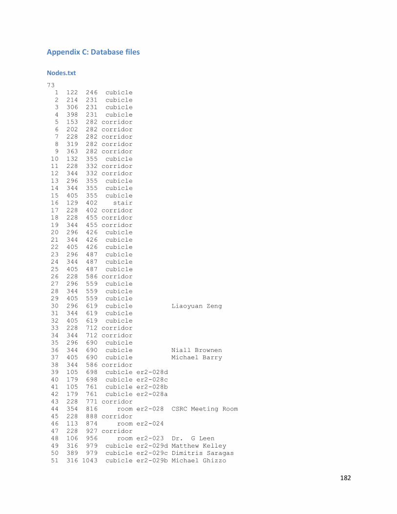
182
Appendix C: Database files
Nodes.txt
73
1 122 246 cubicle
2 214 231 cubicle
3 306 231 cubicle
4 398 231 cubicle
5 153 282 corridor
6 202 282 corridor
7 228 282 corridor
8 319 282 corridor
9 363 282 corridor
10 132 355 cubicle
11 228 332 corridor
12 344 332 corridor
13 296 355 cubicle
14 344 355 cubicle
15 405 355 cubicle
16 129 402 stair
17 228 402 corridor
18 228 455 corridor
19 344 455 corridor
20 296 426 cubicle
21 344 426 cubicle
22 405 426 cubicle
23 296 487 cubicle
24 344 487 cubicle
25 405 487 cubicle
26 228 586 corridor
27 296 559 cubicle
28 344 559 cubicle
29 405 559 cubicle
30 296 619 cubicle Liaoyuan Zeng
31 344 619 cubicle
32 405 619 cubicle
33 228 712 corridor
34 344 712 corridor
35 296 690 cubicle
36 344 690 cubicle Niall Brownen
37 405 690 cubicle Michael Barry
38 344 586 corridor
39 105 698 cubicle er2-028d
40 179 698 cubicle er2-028c
41 105 761 cubicle er2-028b
42 179 761 cubicle er2-028a
43 228 771 corridor
44 354 816 room er2-028 CSRC Meeting Room
45 228 888 corridor
46 113 874 room er2-024
47 228 927 corridor
48 106 956 room er2-023 Dr. G Leen
49 316 979 cubicle er2-029d Matthew Kelley
50 389 979 cubicle er2-029c Dimitris Saragas
51 316 1043 cubicle er2-029b Michael Ghizzo
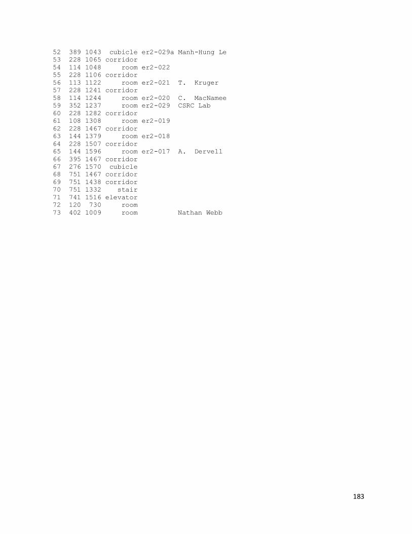
183
52 389 1043 cubicle er2-029a Manh-Hung Le
53 228 1065 corridor
54 114 1048 room er2-022
55 228 1106 corridor
56 113 1122 room er2-021 T. Kruger
57 228 1241 corridor
58 114 1244 room er2-020 C. MacNamee
59 352 1237 room er2-029 CSRC Lab
60 228 1282 corridor
61 108 1308 room er2-019
62 228 1467 corridor
63 144 1379 room er2-018
64 228 1507 corridor
65 144 1596 room er2-017 A. Dervell
66 395 1467 corridor
67 276 1570 cubicle
68 751 1467 corridor
69 751 1438 corridor
70 751 1332 stair
71 741 1516 elevator
72 120 730 room
73 402 1009 room Nathan Webb
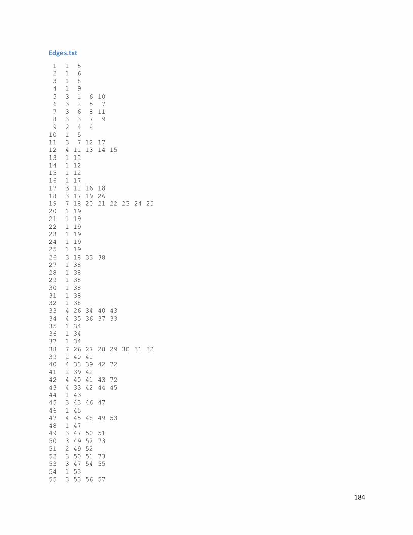
184
Edges.txt
1 1 5
2 1 6
3 1 8
4 1 9
5 3 1 6 10
6 3 2 5 7
7 3 6 8 11
8 3 3 7 9
9 2 4 8
10 1 5
11 3 7 12 17
12 4 11 13 14 15
13 1 12
14 1 12
15 1 12
16 1 17
17 3 11 16 18
18 3 17 19 26
19 7 18 20 21 22 23 24 25
20 1 19
21 1 19
22 1 19
23 1 19
24 1 19
25 1 19
26 3 18 33 38
27 1 38
28 1 38
29 1 38
30 1 38
31 1 38
32 1 38
33 4 26 34 40 43
34 4 35 36 37 33
35 1 34
36 1 34
37 1 34
38 7 26 27 28 29 30 31 32
39 2 40 41
40 4 33 39 42 72
41 2 39 42
42 4 40 41 43 72
43 4 33 42 44 45
44 1 43
45 3 43 46 47
46 1 45
47 4 45 48 49 53
48 1 47
49 3 47 50 51
50 3 49 52 73
51 2 49 52
52 3 50 51 73
53 3 47 54 55
54 1 53
55 3 53 56 57
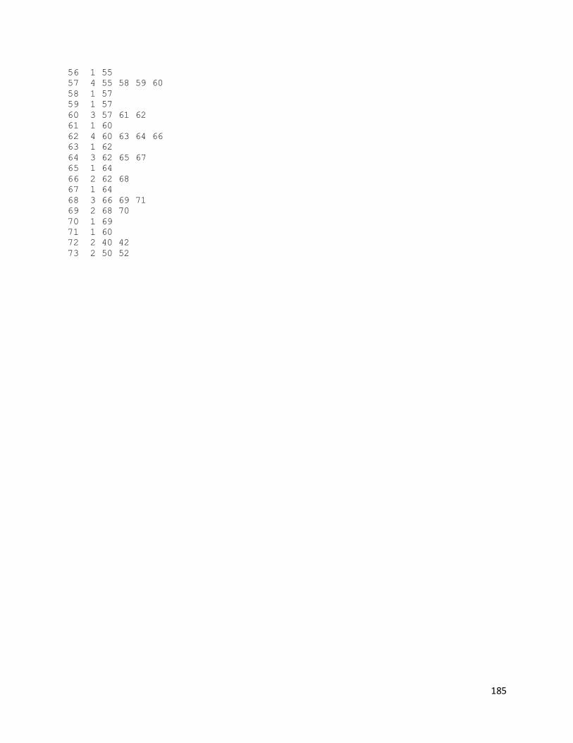
185
56 1 55
57 4 55 58 59 60
58 1 57
59 1 57
60 3 57 61 62
61 1 60
62 4 60 63 64 66
63 1 62
64 3 62 65 67
65 1 64
66 2 62 68
67 1 64
68 3 66 69 71
69 2 68 70
70 1 69
71 1 60
72 2 40 42
73 2 50 52
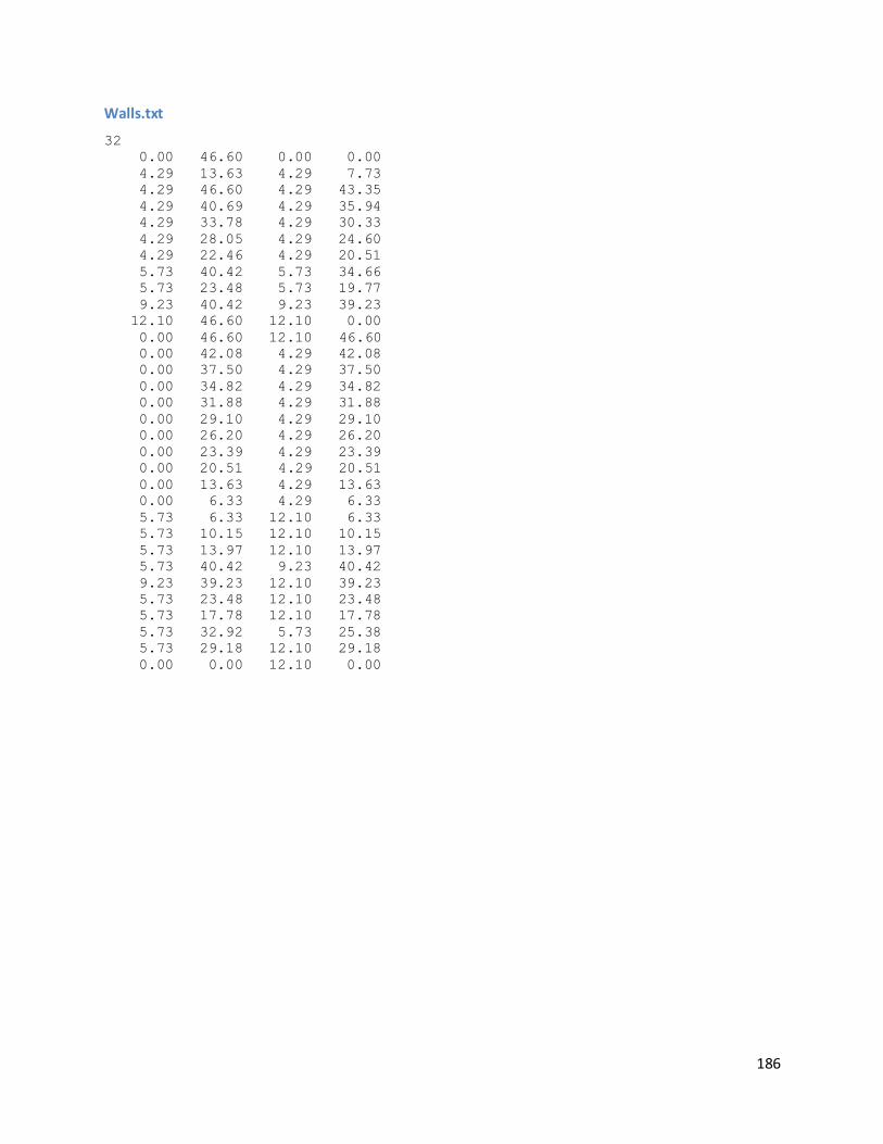
186
Walls.txt
32
0.00 46.60 0.00 0.00
4.29 13.63 4.29 7.73
4.29 46.60 4.29 43.35
4.29 40.69 4.29 35.94
4.29 33.78 4.29 30.33
4.29 28.05 4.29 24.60
4.29 22.46 4.29 20.51
5.73 40.42 5.73 34.66
5.73 23.48 5.73 19.77
9.23 40.42 9.23 39.23
12.10 46.60 12.10 0.00
0.00 46.60 12.10 46.60
0.00 42.08 4.29 42.08
0.00 37.50 4.29 37.50
0.00 34.82 4.29 34.82
0.00 31.88 4.29 31.88
0.00 29.10 4.29 29.10
0.00 26.20 4.29 26.20
0.00 23.39 4.29 23.39
0.00 20.51 4.29 20.51
0.00 13.63 4.29 13.63
0.00 6.33 4.29 6.33
5.73 6.33 12.10 6.33
5.73 10.15 12.10 10.15
5.73 13.97 12.10 13.97
5.73 40.42 9.23 40.42
9.23 39.23 12.10 39.23
5.73 23.48 12.10 23.48
5.73 17.78 12.10 17.78
5.73 32.92 5.73 25.38
5.73 29.18 12.10 29.18
0.00 0.00 12.10 0.00